Measuring the socio-economic background of students and its effect on achievement in PISA 2000 and PISA 2003

Wolfram Schulz Australian Council for Educational Research

Melbourne/Australia schulz@acer.edu.au

Paper prepared for the Annual Meetings of the American Educational Research Association in San Francisco, 7-11 April 2005.

Abstract

One of the consistent findings of educational research studies is the effect of the students’ family socio-economic background on their learning achievement. Consequently, international comparative studies emphasise the role of socio-economic background for determining learning outcomes. In particular, PISA results have been used to describe how different structures of the educational system can mediate the impact of socio-economic family background on performance with comprehensive systems generally providing more equity in educational opportunities.

Given the cyclical nature of the PISA study, it is of interest to observe changes in the relationship between socio-economic background and student performance. However, in order to measure the change in a relationship between two variables over time, one needs to rely on the same (or at least very similar) measures for both constructs. Furthermore, there are some concerns regarding the validity of student reports on family background.

This paper addresses the issue of measuring socio-economic background in the context of the OECD PISA study. It describes the computation of a composite index of “Economic, Social and Cultural Status” derived from occupational status of parents, educational level of parents and home possessions for the first two PISA cycles. It also shows differences in the relationship between socio-economic background and student performance, both using single-level and multi-level analyses and compares student and parent reports on occupation and education in order to explore the validity of these measures.

Socio-economic status and student performance

Socio-economic status (SES) is an important explanatory factor in many different disciplines like health, child development and educational research. Research has shown that socioeconomic status is associated with health, cognitive and socio-emotional outcomes (Bradley and Corwyn, 2002).

In general, educational outcomes have been shown to be influenced by family background in many different and complex ways (Saha, 1997). For example, the socio-economic status of families has been consistently found to be an important variable in explaining variance in student achievement. Socio-economic background may affect learning outcomes in numerous ways: From the outset, parents with higher socio-economic status are able to provide their children with the (often necessary) financial support and home resources for individual learning. They are also more likely to provide a more stimulating home environment to promote cognitive development.

At the level of educational providers, students from high-SES families are also more likely to attend better schools, in particular in countries with differentiated (or "tracked") educational systems, strong segregation in the school system according to neighbourhood factors and/or clear advantages of private over public schooling (as for example in many developing countries). Socio-economic background measures have been used to control the effects of school characteristics on performance dates: Coleman and others (1966) as well as Jencks (1972) claimed that schools were not major determinants of a child’s achievement, particularly when contrasted with the influences of family background on student outcomes.1

When analysing school-level effects of social intake, the question arises how socio-economic status should be measured at the school level: Though some researchers argue against the use of aggregated SES from student samples (see for example Sirin, 2005), alternative school-level measures like participation in free lunch programmes or neighbourhood SES census data are also viewed as inappropriate (see Hauser, 1994). Furthermore, school-level SES data from other sources would most likely be incomparable across countries. In view of the importance of including social intake as a variable in the analysis of student performance, most national and international studies of educational achievement typically rely on aggregated student data as school-level estimates of SES.

Though there is a relative consensus that socio-economic status is represented by income, education and occupation (Gottfried, 1985; Hauser, 1994) and that using all three of them is better than using only one (White, 1982), there is no agreement among researchers which measures should be used in the analysis (Entwisle and Astone, 1994; Hauser, 1994). And whereas some argue that it is better to use a composite measure, others prefer to use single indicators for each component. Furthermore, there are different preferred ways of how to create composite SES measures (Mueller and Parcel, 1981; Gottfried, 1985).

1 Though it should be noted that other researchers (see for example Mayeske et al., 1972) have

argued that social intake in conjunction with school-related variables should rather be viewed as "school factors" than "student background factors".

Differences in the use of measures have often led to quite different results regarding this relationship between SES and student achievement (White, 1982; Sirin, 2005). As Keeves and Saha (1992, p. 166) point out it is clear that adolescents should not be asked about parental income. Alternatively, family wealth (as measured by assets) is often cited as an even better measure of resources than income (Bradley and Corwyn, 2002, p. 372). Based on the notion of assets as good measure of capital, Filmer and Pritchett (1999) propose using household assets to create a socio-economic index that can be validly used in cross-national research.2

In international studies additional caveats are imposed on the validity of background measures and the cross-national comparability of family background measures is an ongoing challenge for researchers in this area (see Buchmann, 2002). Clearly, in international comparative research requires the collection of comparable SES measures across countries.

Student reports on parental education in international research have often suffered from high levels of non-response and a lack of comparability across countries. Recent studies (like PISA) have started to use the International Standard Classification of Education (ISCED) in order to enhance the comparability of data on parental education (OECD, 1999). Higher levels of non-response and the uncertain quality of student-derived data are the most salient concerns regarding the measurement of parental education.

Whereas earlier IEA studies like the First International Mathematics Study (FIMS) collected student data on parental occupation, later studies like the IEA Reading Literacy Study or TIMSS did not continue this practice but instead relied on student reports on parental education and household items as measures of SES.3 The OECD PISA study uses the ISCO classification (ILO, 1990) to code open-ended student responses on father's and mother's occupation which in turn are scored using the International Socio-economic Index of occupational status (SEI) to obtain socio-economic measures (Ganzeboom, de Graaf and Treiman, 1992).

International studies of educational achievement have often made use of student reports on household items as measures of family capital (see Buchmann, 2002). Student reports on the number of books at home are often taken as proxies of SES in analyses of IEA data (see an example in Raudenbush, Cheong and Fotiu, 1996). However, there are concerns regarding the meaning of this variable in different cultural context, in particular in Asian countries.

2 Other measures of socio-economic background, typically not used in international educational

research but also proposed in the literature, are associated with the concepts of social capital (Coleman, 1988) or cultural capital (Bourdieux and Passeron, 1977). One example is the quality of parent-child communication, which is reported to correlate with student performance (see Howerton, Enger and Cobbs, 1993). Other examples include collecting data about student or parent participation in, and preferences for, cultural activities as going to concerts, listening to music, or reading literature (see for example DiMaggio, 1982).

3 It should be noted that collecting student data on parental occupation requires considerable additional resources in order to undertake the coding of open-ended responses which may explain the omission of this aspect in some educational studies.

Data and methods

The OECD PISA study assesses the academic performance of 15-year-old students. In the first assessment in 2000 (with reading as a major domain, mathematics and science as minor domains) 28 OECD member countries and four non-OECD countries participated in the study (see OECD, 2001). An additional data collection in 11 non-OECD countries took place in 2001 (see OECD, 2002). The second assessment in 2003 (with mathematics as major, reading, science and problem solving as minor domains) was carried out in 30 OECD countries and 11 non-OECD countries (OECD, 2004). Currently, the third assessment of science literacy (with reading and mathematics as minor domains) is being carried out in over 50 countries.

For the main study, in each country a nationally representative sample with a minimum of around 4500 students were selected in a two-stage sampling process. In some countries subgroups or regions were over-sampled and larger sample sizes were obtained. In each country schools were sampled proportional to size and (on average 35) 15-year-old students were randomly selected within each school.4 The sampling plan for each country had to be approved by the International Sampling Referee to guarantee that the procedures were the same in all countries. PISA sampling standards require a minimum of 85 percent school participation rate and a participation rate of 80 percent within schools (see technical descriptions of the PISA study in Adams and Wu, 2002; OECD, 2005).5

The following instruments are regularly used to collect data in the OECD PISA study:

• Students are assessed with a 2-hour rotated test design that includes an extensive test on the major domain (2000: Reading, 2003: Mathematics, 2006: Science) and smaller subtests for minor domains (alternating mathematics, reading and science as well as problem solving as additional area of assessment in 2003). All domains are linked through the use of common test items across booklets and plausible values are computed as student proficiency estimates. For each domain, sub-sets of link items provide the basis for measuring trends.

• The student questionnaire includes questions on student characteristics, home background, educational career, school/classroom climate, learning behaviour and self-related cognitions in the area of the major domain (reading, mathematics or science).

• The school questionnaire collects data on the school characteristics and learning environment and is addressed to the school principal.

The data used for the analyses presented in this paper were collected during the main data collections in 2000 and 2003 and the field trial for PISA 2006, which was carried out in 2005. This paper will describe the use of socio-economic measures in PISA and explore their stability over time as well as the validity of these measures:

• In the first section it describes the construction of the composite (socio-economic) index of "Economic, Social and Cultural Status" (ESCS) in PISA.

4 In a few very small countries all 15-year-old students in the target population were assessed. 5 Data from the first two PISA cycles in 2000 (with reading as its major domain) and 2003 (with

mathematics as its major domain) are available and can be used for secondary analyses (http://pisaweb.acer.edu.au/oecd/oecd_pisa_data.html).

• The second section explores the stability of socio-economic measures between the two first PISA cycles (2000 and 2003). The way of constructing the socio-economic composite used in the first cycle was somewhat modified in PISA 2003 but the modified index could be recomputed for PISA 2000. Here, country means from 2000 and 2003 will be compared in order to explore the degree of stable measures over time.

• The third section compares the relationship between socio-economic status and student performance across the first two cycles. It reviews to what extent different relationships were found in the first two PISA cycles. Multivariate (single-level and multi-level) models will be used in the analyses.

• The last section reviews the validity of student-reported socio-economic measures based on comparisons between student data and data collected from parent questionnaires administered during the field trial for PISA 2006. Here, the degree of correspondence (percentage and mean comparisons, correlations) between socio-economic measures from different sources is used to review the validity of the measures used in PISA. It also explores to what extent using parent questionnaire data might provide different results from those obtained when using student questionnaire data.

Student enrolled in special education programmes were assessed with a special one-hour test booklet and (typically) did not provide any student questionnaire data. Therefore, students from these programmes did not have any data on family backgrond and were excluded from the analyses in this paper. Standard errors from single-level analyses were computed using replication techniques (Fay's variant of Balanced Repeated Replication).

Constructing the ESCS index in PISA

The ESCS index used in PISA is derived from three family background variables: the highest level of parental education among the two parents (in number of years of education according to the ISCED classification), the highest parental occupation among the two parents (SEI scores) and the number of home possessions.

Occupational data for both the student’s father and student’s mother were obtained by asking open-ended questions. The responses were coded to four-digit ISCO codes (ILO, 1990) and then mapped to Ganzeboom et al’s SEI index (Ganzeboom, de Graaf and Treiman, 1992). Three indices are obtained from these scores: Recoding of ISCO codes into SEI results in scores for the Mother's occupational status (BMMJ) and Father's occupational status (BFMJ). The Highest Occupational Level of Parents (HISEI) corresponds to the higher SEI score of either parent or to the only available parent's SEI score. Higher scores of SEI indicate higher level of occupational status.

Parental education was asked in categories following the ISCED classification (OECD 1999). Indices on parental education are constructed by recoding educational qualifications into the following categories: (0) None, (1) ISCED 1 (primary education), (2) ISCED 2 (lower secondary), (3) ISCED Level 3B or 3C (vocational/pre-vocational upper secondary), (4) ISCED 3A (upper secondary) and/or ISCED 4 (non-tertiary post-secondary), (5) ISCED 5B (vocational tertiary), (6) ISCED 5A, 6 (theoretically oriented tertiary and post-graduate). The higher index

scores of either parent were then recoded into estimated years of schooling (PARED).6

In PISA 2003, students reported the availability of 13 different household items at home (in PISA 2000, the availability of 12 items). An index of home possessions was derived as a summary index of all household items plus a dummy variable indicating more than 100 books (derived from a separate question on the number of books at home). The items were scored as "dummy variables" so that positive IRT scores (Weighted Likelihood Estimates) indicate higher numbers of home possessions. The items measuring home possessions are shown in Table 1.

Table 1 PISA items measuring home possessions*

Which of the following do you have in your home?

1) Desk for study? 2) A room of your own? 3) A quiet place to study? 4) A computer you can use for school work (only PISA 2003) 5) Educational software 6) A link to the Internet 7) Your own calculator? (only PISA 2003) 8) Classic literature (e.g., <Shakespeare>)? 9) Books of poetry? 10) Works of art (e.g., paintings)? 11) Books to help with your school work? (in PISA 2000: Textbooks) 12) A dictionary? 13) A dishwasher?

How many books are there in your home?

14) More than 100 books (recoded from categories) * The number of books at home was asked in categories. Expressions in <> are adapted to national

context.

Using these three components for deriving a composite index of socio-economic status reflects the general consensus that this construct is best represented by education, occupational status and economic means. As no direct income measure can be obtained from the PISA context questionnaires, student reports on household items are used as approximate measures of family wealth.

Missing values for students with one missing response and two valid responses were imputed as predicted values plus a random component (r(O, σe)):

( )emiss rXbXbaY σ,02211 +++=

Country-specific regression parameters for predicting missing values (a, b1, b2, σe) and the error variance σe were estimated from a regression of the observed values of Yobs on X1 and X2 for all cases without any missing values. The random component r(O, σe) was computed as random draws from normal distributions with a mean of 0 and a variance of σe within each participating country. 6 A mapping of ISCED levels to years of schooling is provided in OECD (2004, p.308).

Variables with imputed values were transformed to an international metric with OECD averages of 0 and OECD standard deviations of 1. These ‘OECD standardised’ variables were used for a principal component analysis applying an OECD population weight giving each OECD country a weight of 1000.

The ESCS scores were obtained as factor scores for the first principal component with 0 being the score of an average ‘OECD student’ and 1 the standard deviation across equally weighted OECD countries. For non-OECD countries, ESCS scores were obtained as

f

SHOMEPODPAREIHISEESCS

εβββ ′+′+′

= 321 (1)

where β1, β2 and β3 are the OECD factor loadings, HISEI', PARED' and HOMEPOS' the variables that were z-standardised for the pooled OECD sample with equal weight and εf is the Eigenvalue of the first principal component.7

Comparing results from Principal Component Analysis within countries (for PISA 2003) shows that patterns of factor loadings are generally similar. Only in a few countries distinct patterns emerge, however, all three components contribute more or less equally to this index with factor loadings ranging from .65 to .85. The reliability for ESCS ranges between .56 and .77 and internal consistency for the pooled OECD sample with equally weighted country data is .69 (see further details in OECD, 2005, Chapter 17).

The stability of socio-economic measures across cycles

Socio-economic background of the parents of 15-year-old students in a country is generally not expected to change much from one PISA cycle to another. Within three years only very moderate but no dramatic changes in the socio-economic composition of the parent population should occur. When substantial changes in socio-economic measures are observed in two subsequent surveys, it is likely that other causes than population change (changes in population coverage, changes of measurement or larger proportions in measurement error) are responsible.

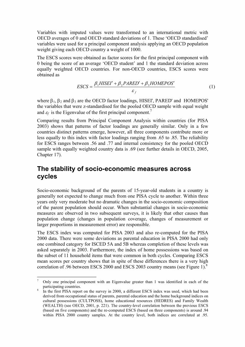
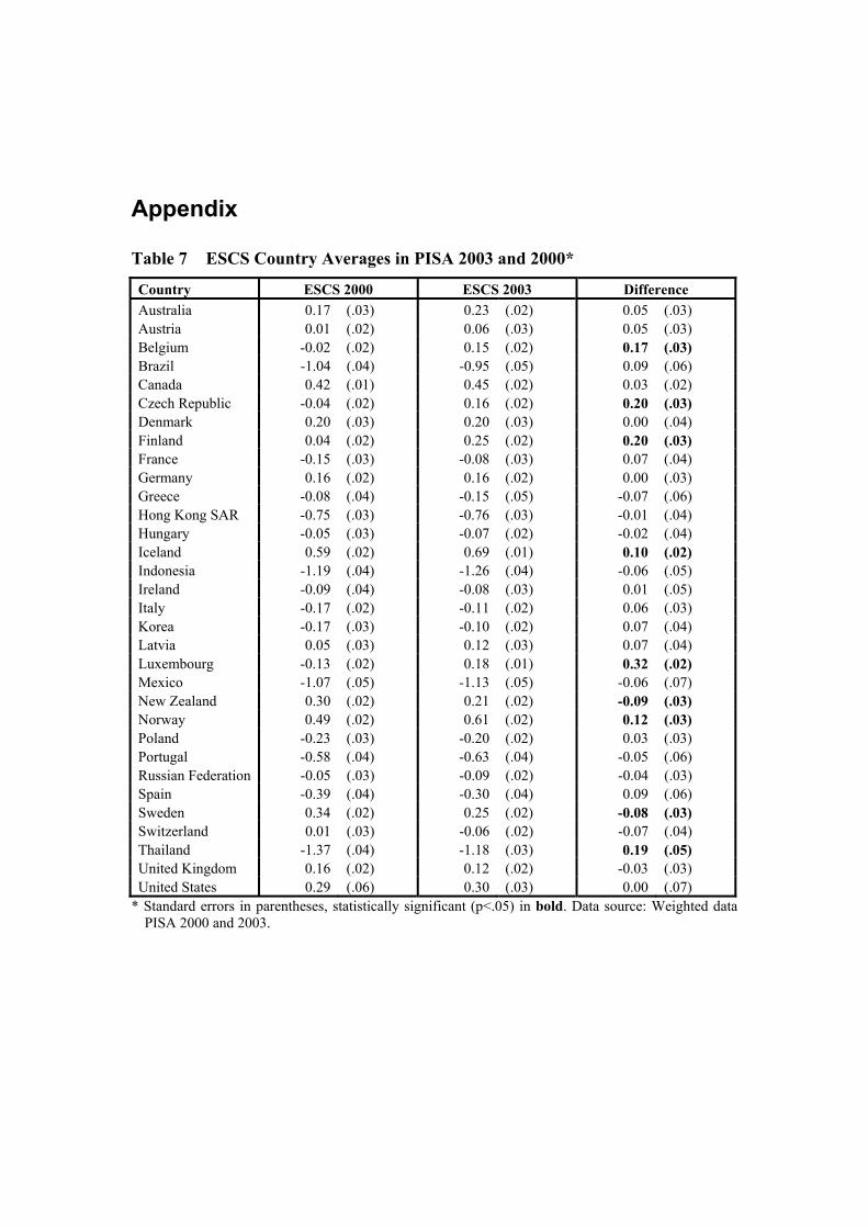
The ESCS index was computed for PISA 2003 and also re-computed for the PISA 2000 data. There were some deviations as parental education in PISA 2000 had only one combined category for ISCED 5A and 5B whereas completion of these levels was asked separately in 2003. Furthermore, the index of home possessions was based on the subset of 11 household items that were common in both cycles. Comparing ESCS mean scores per country shows that in spite of these differences there is a very high correlation of .96 between ESCS 2000 and ESCS 2003 country means (see Figure 1).8

7 Only one principal component with an Eigenvalue greater than 1 was identified in each of the

participating countries. 8 In the first PISA report on the survey in 2000, a different ESCS index was used, which had been

derived from occupational status of parents, parental education and the home background indices on cultural possessions (CULTPOSS), home educational resources (HEDRES) and Family Wealth (WEALTH) (see OECD, 2001, p. 221). The country-level correlation between the previous ESCS (based on five components) and the re-computed ESCS (based on three components) is around .94 within PISA 2000 country samples. At the country level, both indices are correlated at .95.

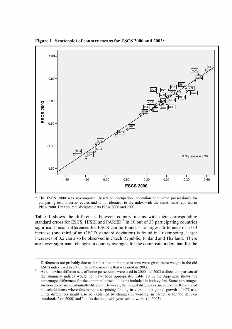
Figure 1 Scatterplot of country means for ESCS 2000 and 2003*

0.600.300.00-0.30-0.60-0.90-1.20-1.50

ESCS 2000

1.00

0.50

0.00

-0.50

-1.00

-1.50

ESC

S 20

03

USA

GBR

THA

CHE

SWE

ESP

PRT

POL

NOR

NZL

NLD

MEX

LUX

LIEKOR

ITA IRL

IDN

ISL

HKG

DEU

FINCZE

CAN

BRA

AUT

R Sq Linear = 0.96

* The ESCS 2000 was re-computed (based on occupation, education and home possessions) for

comparing results across cycles and is not identical to the index with the same name reported in PISA 2000. Data source: Weighted data PISA 2000 and 2003.

Table 1 shows the differences between country means with their corresponding standard errors for ESCS, HISEI and PARED.9 In 10 out of 33 participating countries significant mean differences for ESCS can be found. The largest difference of a 0.3 increase (one third of an OECD standard deviation) is found in Luxembourg, larger increases of 0.2 can also be observed in Czech Republic, Finland and Thailand. There are fewer significant changes in country averages for the composite index than for the

Differences are probably due to the fact that home possessions were given more weight in the old ESCS index used in 2000 than in the new one that was used in 2003.

9 As somewhat different sets of home possessions were used in 2000 and 2003 a direct comparison of the summary indices would not have been appropriate. Table 10 in the Appendix shows the percentage differences for the common household items included in both cycles. Some percentages for household are substantially different. However, the largest differences are found for ICT-related household items where this is not a surprising finding in view of the global growth of ICT use. Other differences might also be explained by changes in wording, in particular for the item on "textbooks" (in 2000) and "books that help with your school work" (in 2003).

single indicators HISEI (significant changes in 14 countries) and PARED (significant changes in 24 countries).

Table 2 Country mean differences in socio-economic indicator variables between PISA 2003 and 2000*

Country ESCS HISEI PARED Australia 0.05 (.03) 0.28 (.71) 0.48 (.07) Austria 0.05 (.03) -2.73 (.63) 1.07 (.09) Belgium 0.17 (.03) 1.53 (.58) 0.68 (.09) Brazil 0.09 (.06) -0.34 (.37) 1.52 (.23) Canada 0.03 (.02) 1.86 (.46) 0.27 (.05) Czech Republic 0.20 (.03) -0.50 (.66) 0.35 (.07) Denmark 0.00 (.04) 0.21 (.59) 0.23 (.10) Finland 0.20 (.03) 0.31 (.69) 1.53 (.08) France 0.07 (.04) 0.19 (.54) -0.10 (.11) Germany 0.00 (.03) -1.39 (.96) -0.39 (.11) Greece -0.07 (.06) -1.40 (.67) 0.28 (.18) Hong Kong SAR -0.01 (.04) -1.20 (.59) -0.07 (.14) Hungary -0.02 (.04) 1.26 (.46) 0.45 (.10) Iceland 0.10 (.02) -2.60 (1.01) 0.62 (.08) Indonesia -0.06 (.05) 0.30 (.71) 0.65 (.20) Ireland 0.01 (.05) -0.14 (.54) 0.39 (.12) Italy 0.06 (.03) 3.32 (.63) 0.75 (.11) Korea 0.07 (.04) 0.41 (.80) 0.53 (.12) Latvia 0.07 (.04) 4.01 (1.50) 0.77 (.10) Luxembourg 0.32 (.02) 3.83 (.41) 1.63 (.11) Mexico -0.06 (.07) -2.62 (.98) 0.37 (.24) Netherlands 0.08 (.04) 0.39 (.66) 0.70 (.11) New Zealand -0.09 (.03) -0.90 (.58) -0.57 (.09) Norway 0.12 (.03) 0.89 (.57) 0.40 (.07) Poland 0.03 (.03) -0.88 (.58) 0.01 (.07) Portugal -0.05 (.06) -1.10 (.87) -0.69 (.20) Russian Federation -0.04 (.03) 0.10 (.66) 0.06 (.06) Spain 0.09 (.06) -0.57 (.88) 0.68 (.18) Sweden -0.08 (.03) 0.30 (.61) -0.12 (.08) Switzerland -0.07 (.04) 0.34 (.76) 0.06 (.09) Thailand 0.19 (.05) 3.20 (.74) 0.95 (.17) United Kingdom -0.03 (.03) -1.62 (.52) -0.14 (.08) United States 0.00 (.07) 2.27 (.89) 0.30 (.18) Median 0.03 0.21 0.39

* Standard errors for sampling in parentheses, statistically significant (p<.05) in bold. Data source: Weighted data PISA 2000 and 2003.

It should be noted that in PISA 2003 more detailed categories were used for post-secondary parental education which may explain (at least some of) the changes in the averages for PARED. For parental occupation, coding procedures may have changed (for example, due to improvements at national centres) and thus have led to different results for HISEI. Both HISEI and PARED have higher median scores in 2003 compared to 2000. The relative stability of the composite index ESCS across the two

cycles can also be attributed to the fact that this index was standardised each time according to the OECD average of equally weighted countries.10

Socio-economic background and student performance

The effect of family background on student performance has received major attention in the reporting of the PISA data from the first two cycles. Both single indicators and composites have been used to explore the effect of socio-economic background on achievement.

Table 3 shows the differences in variance explanation between (single-level) regression models using only a composite index (ESCS) and alternative models using the three indicators (parental occupation, parental education and household possessions) separately. In most countries there are no or only smaller differences between in the variance explanation of the two models. However, in a few countries, in particular in Portugal, using single indicators as predictors explains considerably more variance in reading performance than including only the composite measure ESCS.

Comparing the explained variance for each model across the two cycles shows that patterns look roughly similar; Northern European and Asian countries tend to have less variance in reading performance explained by socio-economic background whereas in countries with highly selective systems like Belgium, Germany and Hungary about 20 percent are explained by socio-economic background. In some countries (most notably in Austria, the Czech Republic and Luxembourg) notable changes in variance explanation between the two cycles can be observed.

10 Please note that in 2000 only 28 OECD countries participated whereas in 2003 Slovak Republic and

Turkey joined as additional OECD countries.

Table 3 Explained variance in reading performance with ESCS versus single indicators (HISEI, PARED, HOMEPOS) as predictors (in percentages)

PISA 2000 PISA 2003 Country Model A Model B Diff. Model A Model B Diff. Australia 18 18 0 14 14 0Austria 14 14 0 21 23 -2Belgium 19 20 -1 23 23 1Brazil 14 15 -1 8 12 -4Canada 12 12 0 10 11 -1Czech Rep. 23 22 1 16 15 0Denmark 16 16 0 16 17 -1Finland 9 9 0 10 10 0France 18 21 -3 20 21 -1Germany 24 24 -1 22 21 1Greece 12 14 -1 11 13 -2Hong Kong 8 8 0 5 7 -2Hungary 26 25 1 22 21 0Iceland 7 7 0 4 4 -1Indonesia 9 11 -2 7 10 -3Ireland 12 14 -2 16 17 -1Italy 10 10 0 14 15 -2Korea 9 9 0 11 12 -2Latvia 9 9 0 8 10 -2Luxembourg 22 28 -6 17 18 -2Mexico 20 20 0 18 20 -3Netherlands 15 15 0 15 16 -1New Zealand 15 14 1 17 19 -2Norway 13 13 0 12 12 0Poland 14 14 0 16 16 0Portugal 18 22 -4 13 18 -5Russian Fed. 10 11 -1 11 12 -1Spain 16 17 -1 11 13 -2Sweden 12 12 0 14 15 0Switzerland 21 21 0 18 18 0Thailand 7 9 -2 10 11 -1United Kingd. 20 20 0 19 19 0United States 20 21 -1 18 18 0Median 14 14 0 14 15 -1

* Data source: Weighted data PISA 2000 and 2003. Model A: Regression of reading performance on occupational status (HISEI), highest parental occupation (PARED) and home possessions (HOMEPOSB). Model B: Regression of reading performance on Economic, Social and Cultural Status (ESCS), Students enrolled in special education programmes were included from the analyses.

Figure 2 Explained variance in reading performance (unique and common variance) in selected PISA countries

0% 5% 10% 15% 20% 25%

Finland 2000

Finland 2003

Germany 2000

Germany 2003

Italy 2000

Italy 2003

Korea 2000Korea 2003

Poland 2000

Poland 2003

Thailand 2001

Thailand 2003

United States 2000

United States 2003

HISEI

PARED

HOMEPOSB

Common

* Data source: Weighted data PISA 2000 and 2003. Regression of reading performance on

occupational status (HISEI), highest parental occupation (PARED) and home possessions (HOMEPOSB). Students enrolled in special education programmes were included from the analyses.

The explained variance can be decomposed into the variance uniquely explained by one factor and the variance proportion that is explained by more than one factor. 11 Figure 2 shows the explained variance components for a selection of PISA countries, based on a regression model for reading performance in 2000 and 2003 with parental occupation (HISEI), parental education (PARED) and home possessions (HOMEPOSB) as predictors. The countries were selected as representing different educational systems and regions.

It is interesting to note that generally half or more of variance in reading performance is explained by more than one of the three factors. Most of the unique variance explanation is typically due to household possessions. Parental occupation contributes a smaller but still sizeable proportion of variance in reading performance (with the exception of Korea), whereas parental education contributes only a very small part to the explained variance (only in Germany this proportion is notably larger). These results show that much of the explained variance in reading performance can be attributed to either parental occupation or education. Including home possessions as third factor increase the variance explanation beyond the explanatory power of the two other factors.

11 Unique variance is the variance explained by each factor in addition to the variance already

explained by the other factors in the model.

Figure 3 Student and school-level effects of ESCS on reading performance

-20 0 20 40 60 80 100 120

Finland

Germany

Italy

Korea

Poland

Thailand

United States

Student-level ESCS 2000

School-level ESCS 2000

Student-level ESCS 2003

School-level ESCS 2003

* Un-standardised regression coefficients from two-level model (SPSS estimates) with fixed effects.

Data source: Data from PISA 2000 and 2003 (with normalised weights at student level).

In addition to single-level regression analyses, two-level models (see Bryk and Raudenbush, 1992) with students nested within schools were estimated where reading performance was regressed on student-level ESCS and aggregated school level ESCS as fixed predictors.12 The un-standardised regression coefficients for single-level models and two-level models for all PISA countries in 2000 and 2003 are shown in Table 11 in the appendix.

Large within-school effects for socio-economic background (as measured by the ESCS index) signal that this factor affects variation within schools, whereas larger effects of the aggregated ESCS index indicate that school-level performance covaries with the social intake of schools. Typically, in countries with comprehensive educational systems, most of the SES effects are found within schools but there are no or only weak effects of school-level SES on performance. Conversely, in countries with selective ("tracked") or socially segregated educational systems school-level effects of social intake tend to be large whereas (due to the socially more homogenous population within schools) student-level effects are rather weak.

Figure 3 shows the un-standardised regression coefficients from the two-level models explaining reading performance for selected PISA countries. Typically, results are

12 Please note that in some PISA countries, sub-units within schools were sampled instead of schools

as administrative units which may affect the estimation of multi-level models. In Austria, the Czech Republic, Hungary and Italy, schools with more than one study programme were split into the units delivering these programmes. In Mexico, schools where instruction is delivered in shifts were split into the corresponding units. The same was done in Brazil, but only in the PISA 2000 assessment. In the French part of Belgium in PISA 2000, in case of multi-campus schools, implantations (campuses) were sampled whereas in the Flemish part, in case of multi-campus schools the larger administrative units were sampled; in PISA 2003 in the French part larger administrative units were sampled and in the Flemish part implantations.

similar though some of the effect sizes in 2003 are statistically significantly from those in 2000. The only drastic change obviously occurred in Poland where in PISA 2000 the between-school effect was similar to Germany (with its highly selective and structured system) whereas in PISA 2003 the between-school effects has diminished substantially. In this particular case the change can be explained with the fundamental educational reform that took place in Poland between the two assessments: The decrease in between-school variance in general and the decrease of the effect of social intake can be interpreted as a reflection of the change from a selective and structured system to a comprehensive one.

In summary, comparing the effects of socio-economic background indicates that roughly similar pictures emerge from the analyses. However, it becomes also clear that there is some (and often statistically significant) variation between the two surveys which may (also) be a consequence of the instability of the measurement of students' socio-economic background.

Validating socio-economic measures in PISA

From the early beginnings of the PISA study, the question of validity of socio-economic student measures has been raised, in particular with regard to the open-ended collection of parental occupation. In the first survey, some countries collected occupational data from parents of sub-samples of PISA students and results showed that in spite of discrepancies between student and parent reports, there was still a relatively high degree of consistency (see Adams and Wu, 2002, p. 268f.). However, these validity studies were carried out on smaller sub-samples during the field trial in only four participating countries.

In the field trial for the PISA main survey in 200613 15 countries collected data through a parent questionnaire that was administered in addition to the student questionnaire. Both students and parents provided open-ended responses regarding the occupation of mother and father (or guardians) and educational parental qualifications. Data from the field trial enable us to compare to what extent parent and student reports are consistent and explore the validity of socio-economic measures in PISA.

One reason for inconsistency is certainly lack of student knowledge but lack of precision in the description, tendency to give socially desirable responses or coding problems can also contribute to deviant codes.14 It needs to be recognised, however, that parent reports might also be biased: Apart from coding problems, lack of precision in the job descriptions and also tendencies to give socially desirable responses might affect the reliability or validity of parent responses.

Comparing the consistency of parent and student reports at different levels of the ISCO categories (see Appendix, Table 12) illustrates that the consistency varies according to the level of coding.15 Not surprisingly, agreement is highest for the major 13 The field trial was carried out in all participating countries between March and September 2005

using convenience samples (roughly representing all major school types and study programmes) of typically 1200 students.

14 It should be noted that double-coding procedures during the field trial data in some of the participating countries indicated a high level of inter-coder reliability.

15 The ISCO classification includes nine major groups, two-digit minor groups and four-digit categories, see ILO, 1990.

occupational groups (higher than 65 in all but two out of 13 countries) and lowest for the single four-digit categories (below 50 percent in five out of 13 countries). Consistencies are generally similar for both mother's and father's occupational data.

Table 4 Correlations between Student Occupational Status Scores from Parent and Student Reports

Occupational Status Country Mother Father Highest Alpha 0.96 0.94 0.93 Beta 0.80 0.79 0.77 Gamma 0.80 0.83 0.79 Delta 0.87 0.84 0.80 Epsilon 0.83 0.76 0.76 Zeta 0.81 0.87 0.79 Eta 0.89 0.91 0.88 Theta 0.57 0.56 0.56 Iota 0.75 0.75 0.72 Kappa 0.73 0.80 0.75 Lambda 0.86 0.81 0.82 Mu 0.86 0.83 0.83 Nu 0.73 0.74 0.73 Xi 0.75 0.78 0.68 Omicron 0.93 0.85 0.86 Median 0.81 0.81 0.79

Data source: Field Trial for PISA 2006.

Table 416 shows the correlations between parent and student SEI scores on parental occupation. The correlation between parent and student variables can be interpreted as a measure of reliability and it can be shown that the reliability of SEI measures across countries is about 0.8. Only in one country ("Theta") considerably lower correlations of below 0.6 can be observed.

Table 13 shows the percentages of agreement between student and parents on educational ISCED levels. It becomes clear that the highest levels of agreement can be found for students whose parents have university level qualifications (ISCED 5A). In about half of the countries the agreement is also quite high for parents with an educational level below general secondary (ISCED 3A, ISCED 4). Typically, agreement is slightly higher for the students' mother's educational level than for their father's education.

In particular, there is lower agreement on vocational tertiary qualifications (ISCED 5B) across countries and also for the combined category of general secondary and non-tertiary post-secondary qualifications (ISCED 3A and 4). This indicates that student often have problems to accurately describe non-university post-secondary qualifications. This finding is not unexpected given the complexity of study programme structures in many educational systems.

16 As the data were collected from convenience samples during the field trial for PISA 2006, country

names are suppressed and Greek letters are used instead.

Table 5 Correlations between Educational Levels from Parent and Student Reports

Occupational Level Country Mother Father Highest Alpha 0.75 0.71 0.72 Beta 0.66 0.68 0.65 Gamma 0.46 0.50 0.45 Delta 0.66 0.71 0.70 Epsilon 0.70 0.66 0.69 Zeta 0.34 0.33 0.29 Eta 0.64 0.63 0.63 Theta 0.72 0.78 0.77 Iota 0.43 0.47 0.43 Kappa 0.52 0.46 0.43 Lambda 0.72 0.69 0.71 Mu 0.63 0.55 0.57 Nu 0.64 0.63 0.63 Xi 0.26 0.29 0.24 Omicron 0.89 0.90 0.90 Median 0.64 0.63 0.63

Data source: Field Trial for PISA 2006.

Table 5 illustrates the degree of correlation between student and parent data on parental education.17 The reliability of the measures on education is lower than the one for occupation, across countries it is only slightly above 0.6. There is also considerable variation in consistency across countries, in some of the national data the reliability for educational measures appears to be particularly low.18 Clearly, student data on parent education have considerably lower overall reliability than student data on parental occupation.

One way to assess the differences between using student reports or parent reports as measures of SES is to estimate regression models explaining student performance with socio-economic background measures from each data source. As student questionnaire background measures highest parental occupation (SEI scores), highest parental education (four-point ISCED index) and home possessions (raw score) were used, as parent questionnaire background measures highest parental occupation (SEI scores), highest parental education (four-point ISCED index) and household income (six categories scored around estimated country median).19

17 The data on parental education were recoded into variables indicating the highest qualification with

four categories: (3) ISCED 5A, University, (2) ISCED 5B, Vocational Tertiary, (1) ISCED 3A, general secondary, combined with ISCED 4, non-tertiary post-secondary and (0) Education below ISCED 3A, general secondary.

18 It should be noted that the country with correlation below 0.3 ("Xi") is also a country where the participation rate for the parent questionnaire was extremely low.

19 In one country ("Eta") the question regarding household income was not administered due to concerns regarding privacy and the data had to be omitted from this part of the analysis.

Table 6 Comparison of variance explanation in science student performance with education, occupation and household possessions/income as predictors (student and parent reports)

Variance uniquely explained by...

Explained variance Highest

Education Highest

Occupation

Home possessions

/Income Country Student Parent Diff. Student Parent Student Parent Student Parent Alpha 25 23 2 1 5 3 2 7 1 Beta 15 18 -3 2 2 3 2 2 2 Gamma 14 12 1 0 2 5 2 2 0 Delta 6 8 -2 0 1 2 1 0 0 Epsilon 11 8 3 1 1 2 2 2 0 Theta 7 16 -8 2 4 0 3 1 9 Iota 6 5 1 1 0 1 2 2 0 Kappa 14 12 1 0 3 6 1 1 0 Lambda 15 8 7 0 2 1 1 9 1 Mu 12 15 -3 0 3 3 1 1 1 Nu 23 21 2 0 0 4 4 8 3 Xi 15 6 9 1 0 4 3 5 0 Omicron 10 18 -8 0 2 8 4 1 2 Theta 26 24 2 3 7 0 0 7 1 Median 14 14 1 1 2 3 2 2 1

Data source: Field Trial for PISA 2006.

Table 6 shows the explained variance (in percentages) overall and uniquely explained by each socio-economic factor. Generally, similar amounts of variance in student performance can be explained using either model. However, whereas in some countries parent-based measures explain more variance, in other countries the reverse happens and student-based measures explain more of the variation in test performance.

Looking at the explained variance unique to socio-economic measures shows a considerable amount of variation. Typically, the variance explanation uniquely due to educational level is higher for measures derived from the parent questionnaire, whereas in most countries the reverse can be observed for measures of occupational status. In most countries, household possessions (reported by students) provide more additional variance explanation over occupation and education than household income (reported by parents).

Generally, it can be concluded that the socio-economic measures from the student questionnaire are able explain similar amount of variance in student achievement as (most likely more reliable) measures derived from parents. From a conceptual point of view parent data would be preferable sources of socio-economic background. But the often much higher levels of non-response for parent questionnaires and general problems with the implementation of parent surveys in many participating countries do not allow the use of this instrument as a standard source of SES data in the PISA study.

Discussion

Measuring socio-economic background in international student surveys is an important challenge. Typically, educational studies employ student questionnaires to obtain data on socio-economic background and three variables (either as single indicators or in combination) can be identified as standard measures of family SES in educational research: (i) parental education, (ii) parental occupation and (iii) household items. These three variables can be viewed as a reasonable representation of the concept of socio-economic status when collecting data from students on home background.

As PISA can show, it is important to provide information about the effects of SES on performance and many of the results have helped to highlight differences in equity in education and describe the way SES interacts with the characteristics of educational systems. But it needs to be recognised that there are some methodological problems with the collection of valid and reliable student background data in international educational research. The analyses in this paper show that care needs to be taken with regard to the interpretation of analyses and future surveys should try to strengthen the measurement approach taken in this study.

The analyses presented in this paper show that PISA succeeded in collecting measures of socio-economic background that can be combined to a composite index with reasonable internal consistency and stability across the first two surveys. Reviewing the stability of the three components, however, indicates that there is some larger than expected variation across cycles, in particular with regard to (non-ICT related) household items. Some of the variation may be due to (minor) format changes across the two cycles and care should be taken to avoid even smaller modifications in future surveys. In PISA 2006, countries include additional country-specific household items in order to strengthen the reliability of the indices derived from this type of indicators.

Analysing the effects of socio-economic background measures on reading performance in the first two PISA cycles with single-level regression modelling reveals roughly similar patterns within countries across the two cycles but in some countries changes in the variance explained by socio-economic background can be observed. Comparing results from regression models using single indicators for parental occupation, parental education and household possessions shows that in a smaller number of countries the composite index explains less variance than using all three components separately.

Decomposing the variance in reading performance explained by (a single-level regression) model using the three components indicate that household possessions typically add more unique variance explanation than parental occupation and education. This observation indicates that student reports on household possessions provide data on family background that are able to explain variation in achievement that is not already predicted with parental occupation and education. Parental education is the variable that usually adds the smallest unique variance explanation.

Using two-level models to explain the reading performance with the socio-economic index ESCS within countries in 2000 and 2003 shows that the effects of ESCS at the student- and school-level can be used to describe characteristics of educational systems in participating countries. When comparing outcomes from 2003 with those

from 2000, effects look relatively similar though in a number of countries (statistically significant) differences are found. The fundamental change in the effects of ESCS on reading performance at student- and school-level in Poland can be explained with the introduction of a comprehensive educational system that was carried out between the two cycles.

Reviewing the consistency of student and parent reports using field trial data from the third cycle confirms that student reports on family background are only partially consistent with parent reports. In particular, student reports on parental education lack precision. While it is relatively easy for students to report whether their parents studied at university, responses about more fine-grained educational qualifications of their parents are often inconsistent. It should be noted that even though there is no "close match" between student and parent reports on occupations either, the (estimated) reliabilities for parental occupation are substantially higher than those for parental education. Using either student- or parent-derived variables in order to estimate effects of socio-economic background on student achievement does not make large differences, though in some countries the use of parent-derived SES measures might lead to an increase in the variance explanation due to socio-economic background.

There is no doubt that from a conceptual point of view it would be preferable to obtain socio-economic measures directly from parents but the implementation of parent questionnaire as a standard source of SES data in PISA is not possible due to response-rate problems and privacy concerns in many participating countries. Therefore, collecting a larger number of student variables on socio-economic family background including parental education, parental occupation as well as household possessions is definitely the only standard approach that is able to maximise what reasonably can be obtained within the scope of international studies in this area.

The analyses presented in this paper show that within PISA countries the effects of socio-economic background measures on student performance across the first two PISA cycles remain mostly unchanged. No fundamentally different conclusions about the relationship between SES and achievement would have been drawn when using data from either survey (with one exception where there is an explanation for the change in the relationship). But there is some variation which might partly be due to problem with measurement and researchers as well as policy-makers are strongly advised not to interpret minor changes in the relationship between SES and performance (for example as possible outcomes of recent policy changes). It needs to be recognised that there is a considerable amount of measurement error associated with student reports on family background which needs to be taken into account when interpreting findings from PISA.

References

Adams, R. and Wu, M. (eds.). (2002). PISA 2000. Technical Report. Paris: OECD Publications.

Bradley, R. H. and Corwyn, R. F. (2002). Socioeconomic Status and Child Development. Annual Review of Psychology, 53:371-99.

Buchmann, C. (2002). Measuring Family Background in International Studies of Education: Conceptual Issues and Methodological Challenges. In: Porter, A. C. and Gamoran, A. (eds.). Methodological Advances in Cross-National Surveys of Educational Achievement (pp. 150-97). Washington, DC: National Academy Press.

Bryk, A. S. and Raudenbush, S. W. (1992). Hierarchical Linear Models: Application and Data Analysis Methods. Newbury Park: SAGE.

Coleman, J. S. et. al. (1966). Equality of educational opportunity. Washington: D.C.U.S. Department of Health, Education and Welfare.

Coleman, J. S. (1988). Social capital in the creation of human capital. American Journal of sociology, 94, 95-120.

DiMaggio, P. (1982). Cultural capital and school success: the impact of status capital participation on the grades of U.S. high school students. American Sociological Review 60: 746-61.

Duncan, G. J. and Magnuson, K. (2003). Off with Hollingshead: Socioeconomic Resources, Parenting, and Child D evelopment. In: M. Bornstein and R. Bradley (Eds.). Socioeconomic Status, parenting, and child development (pp. 83–106). Mahwah, NJ: Lawrence Erlbaum.

Entwistle, D. R. and Astone, N. M. (1994). Some Practical Guidelines for Measuring Youth’s Race/Ethnicity and Socioeconomic Status. Child Development, 65, 1521-1540.

Filmer, D. and Pritchett, L. (1999). The effect of household wealth on educational attainment: evidence from 35 countries. Population Development Review, 25, 85-120.

Ganzeboom, H.B.G., de Graaf, P.M., and Treiman, D.J. (1992). A standard international socio-economic index of occupational status. Social Science Research, 21, 1-56.

Gottfried, A. W. (1985). Measures of Socioeconomic Status in Child Development Research: Data and Recommendations. Merrill-Palmer Quarterly, 31:1, 85-92.

Hauser, R. M. (1994). Measuring Socioeconomic Status in Studies of Child Development. Child Development, 65, 1541-1545.

Howerton, D. L., Enger, J. M., and Cobbs, C. R. (1993). Parental Verbal Interaction and Academic Achievement for At-Risk Adolescent Black Males. Paper presented at the annual meeting of the Mid-South Educational Research Association, November 10, New Orleans, LA.

International Labour Organisation (1990). International Standard Classification of Occupations: ISCO-88. Geneva: International Labour Office.

Jencks, C. (1972). Inequality: A reassessment of the effect of family and schooling. New York: Basic Books.

Keeves, J. P. and Saha, L. J. (1992). Home background factors and educational outcomes. In: Keeves, J. P. (ed.). The IEA Study of Science III: Changes in Science Education and Achievement: 1970-1984 (pp. 165-186). Oxford: Pergamon.

Mayeske et. al. (1972). A Study of Our Nation's Schools. Washington. D.C.: US Department of Health, Education and Welfare.

Mueller, C. W. and Parcel, T. L. (1981). Measures of Socioeconomic Status: Alternatives and Recommendations. Child Development, 52, 13-30.

Organisation for Economic Co-operation and Development (1999). Classifying Educational Programmes. Manual for ISCED-97 Implementation in OECD Countries. Paris: OECD Publications.

Organisation for Economic Co-operation and Development (2001). Knowledge and Skills for Life. First Results from PISA 2000. Paris: OECD Publications

Organisation for Economic Co-operation and Development (2002). Literacy Skills for the World of Tomorrow – Further Results from PISA 2000. Paris: OECD Publications

Organisation for Economic Co-operation and Development (2004). Learning for Tomorrow’s World – First Results from PISA 2003. Paris: OECD Publications

Organisation for Economic Co-operation and Development (2005). PISA 2003. Technical Report. Paris: OECD Publications.

Raudenbush, S. W., Cheong, Y. F. and Fotiu, R. P. (1996). Social Inequality, Social Segregation, and Their Relationship to Reading Literacy in 22 Countries. In: Binkley, M, Rust, K. and Williams, T. (Eds.). Reading Literacy in an International Perspective (pp. 3- 62). Washington D.C.: NCES.

Sirin, S. R. (2005). Socioeconomic Status and Academic Achievement: A Meta-Analytic Review of Research. Review of Educational Research, 75:3, 417-453.

White, K. R. (1982).The relation between socioeconomic status and educational achievement. Psychological Bulletin, 91(3), 461-81.

Appendix

Table 7 ESCS Country Averages in PISA 2003 and 2000*

Country ESCS 2000 ESCS 2003 Difference Australia 0.17 (.03) 0.23 (.02) 0.05 (.03) Austria 0.01 (.02) 0.06 (.03) 0.05 (.03) Belgium -0.02 (.02) 0.15 (.02) 0.17 (.03) Brazil -1.04 (.04) -0.95 (.05) 0.09 (.06) Canada 0.42 (.01) 0.45 (.02) 0.03 (.02) Czech Republic -0.04 (.02) 0.16 (.02) 0.20 (.03) Denmark 0.20 (.03) 0.20 (.03) 0.00 (.04) Finland 0.04 (.02) 0.25 (.02) 0.20 (.03) France -0.15 (.03) -0.08 (.03) 0.07 (.04) Germany 0.16 (.02) 0.16 (.02) 0.00 (.03) Greece -0.08 (.04) -0.15 (.05) -0.07 (.06) Hong Kong SAR -0.75 (.03) -0.76 (.03) -0.01 (.04) Hungary -0.05 (.03) -0.07 (.02) -0.02 (.04) Iceland 0.59 (.02) 0.69 (.01) 0.10 (.02) Indonesia -1.19 (.04) -1.26 (.04) -0.06 (.05) Ireland -0.09 (.04) -0.08 (.03) 0.01 (.05) Italy -0.17 (.02) -0.11 (.02) 0.06 (.03) Korea -0.17 (.03) -0.10 (.02) 0.07 (.04) Latvia 0.05 (.03) 0.12 (.03) 0.07 (.04) Luxembourg -0.13 (.02) 0.18 (.01) 0.32 (.02) Mexico -1.07 (.05) -1.13 (.05) -0.06 (.07) New Zealand 0.30 (.02) 0.21 (.02) -0.09 (.03) Norway 0.49 (.02) 0.61 (.02) 0.12 (.03) Poland -0.23 (.03) -0.20 (.02) 0.03 (.03) Portugal -0.58 (.04) -0.63 (.04) -0.05 (.06) Russian Federation -0.05 (.03) -0.09 (.02) -0.04 (.03) Spain -0.39 (.04) -0.30 (.04) 0.09 (.06) Sweden 0.34 (.02) 0.25 (.02) -0.08 (.03) Switzerland 0.01 (.03) -0.06 (.02) -0.07 (.04) Thailand -1.37 (.04) -1.18 (.03) 0.19 (.05) United Kingdom 0.16 (.02) 0.12 (.02) -0.03 (.03) United States 0.29 (.06) 0.30 (.03) 0.00 (.07)

* Standard errors in parentheses, statistically significant (p<.05) in bold. Data source: Weighted data PISA 2000 and 2003.

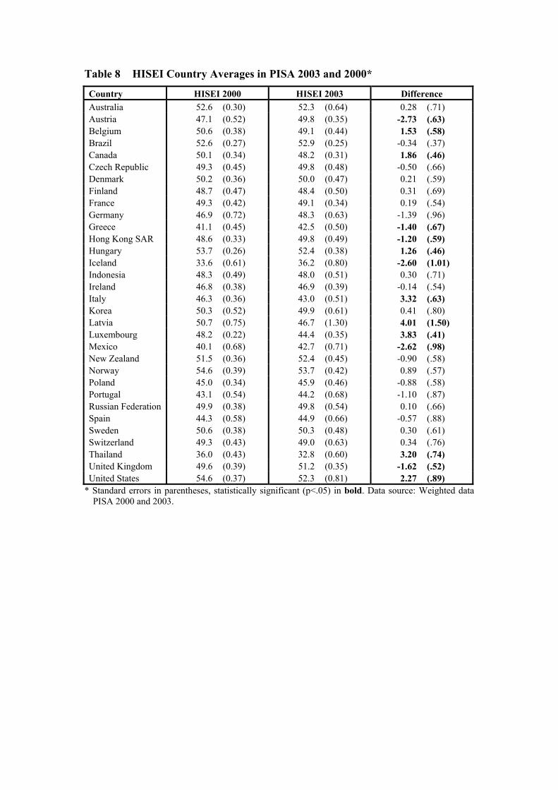
Table 8 HISEI Country Averages in PISA 2003 and 2000*

Country HISEI 2000 HISEI 2003 Difference Australia 52.6 (0.30) 52.3 (0.64) 0.28 (.71) Austria 47.1 (0.52) 49.8 (0.35) -2.73 (.63) Belgium 50.6 (0.38) 49.1 (0.44) 1.53 (.58) Brazil 52.6 (0.27) 52.9 (0.25) -0.34 (.37) Canada 50.1 (0.34) 48.2 (0.31) 1.86 (.46) Czech Republic 49.3 (0.45) 49.8 (0.48) -0.50 (.66) Denmark 50.2 (0.36) 50.0 (0.47) 0.21 (.59) Finland 48.7 (0.47) 48.4 (0.50) 0.31 (.69) France 49.3 (0.42) 49.1 (0.34) 0.19 (.54) Germany 46.9 (0.72) 48.3 (0.63) -1.39 (.96) Greece 41.1 (0.45) 42.5 (0.50) -1.40 (.67) Hong Kong SAR 48.6 (0.33) 49.8 (0.49) -1.20 (.59) Hungary 53.7 (0.26) 52.4 (0.38) 1.26 (.46) Iceland 33.6 (0.61) 36.2 (0.80) -2.60 (1.01) Indonesia 48.3 (0.49) 48.0 (0.51) 0.30 (.71) Ireland 46.8 (0.38) 46.9 (0.39) -0.14 (.54) Italy 46.3 (0.36) 43.0 (0.51) 3.32 (.63) Korea 50.3 (0.52) 49.9 (0.61) 0.41 (.80) Latvia 50.7 (0.75) 46.7 (1.30) 4.01 (1.50) Luxembourg 48.2 (0.22) 44.4 (0.35) 3.83 (.41) Mexico 40.1 (0.68) 42.7 (0.71) -2.62 (.98) New Zealand 51.5 (0.36) 52.4 (0.45) -0.90 (.58) Norway 54.6 (0.39) 53.7 (0.42) 0.89 (.57) Poland 45.0 (0.34) 45.9 (0.46) -0.88 (.58) Portugal 43.1 (0.54) 44.2 (0.68) -1.10 (.87) Russian Federation 49.9 (0.38) 49.8 (0.54) 0.10 (.66) Spain 44.3 (0.58) 44.9 (0.66) -0.57 (.88) Sweden 50.6 (0.38) 50.3 (0.48) 0.30 (.61) Switzerland 49.3 (0.43) 49.0 (0.63) 0.34 (.76) Thailand 36.0 (0.43) 32.8 (0.60) 3.20 (.74) United Kingdom 49.6 (0.39) 51.2 (0.35) -1.62 (.52) United States 54.6 (0.37) 52.3 (0.81) 2.27 (.89)

* Standard errors in parentheses, statistically significant (p<.05) in bold. Data source: Weighted data PISA 2000 and 2003.

Table 9 PARED Country Averages in PISA 2003 and 2000*

Country PARED 2000 PARED 2003 Difference Australia 13.05 (0.04) 12.57 (0.06) 0.48 (.07) Austria 13.05 (0.07) 11.98 (0.06) 1.07 (.09) Belgium 13.53 (0.06) 12.85 (0.07) 0.68 (.09) Brazil 10.64 (0.18) 9.12 (0.15) 1.52 (.23) Canada 14.53 (0.04) 14.26 (0.03) 0.27 (.05) Czech Republic 13.71 (0.05) 13.37 (0.05) 0.35 (.07) Denmark 14.00 (0.08) 13.77 (0.06) 0.23 (.10) Finland 13.61 (0.04) 12.08 (0.07) 1.53 (.08) France 11.93 (0.08) 12.03 (0.08) -0.10 (.11) Germany 12.93 (0.09) 13.33 (0.07) -0.39 (.11) Greece 12.97 (0.14) 12.70 (0.12) 0.28 (.18) Hong Kong SAR 9.69 (0.10) 9.75 (0.10) -0.07 (.14) Hungary 12.66 (0.06) 12.21 (0.08) 0.45 (.10) Iceland 14.43 (0.05) 13.81 (0.06) 0.62 (.08) Indonesia 9.67 (0.13) 9.01 (0.15) 0.65 (.20) Ireland 12.50 (0.07) 12.11 (0.10) 0.39 (.12) Italy 12.52 (0.07) 11.76 (0.08) 0.75 (.11) Republic of Korea 12.47 (0.08) 11.94 (0.08) 0.53 (.12) Latvia 14.33 (0.08) 13.56 (0.06) 0.77 (.10) Luxembourg 13.43 (0.07) 11.80 (0.08) 1.63 (.11) Mexico 9.59 (0.18) 9.22 (0.16) 0.37 (.24) New Zealand 13.47 (0.06) 14.05 (0.06) -0.57 (.09) Norway 14.59 (0.04) 14.18 (0.05) 0.40 (.07) Poland 12.45 (0.05) 12.44 (0.05) 0.01 (.07) Portugal 9.24 (0.16) 9.93 (0.13) -0.69 (.20) Russian Federation 13.26 (0.04) 13.20 (0.04) 0.06 (.06) Spain 11.11 (0.12) 10.43 (0.13) 0.68 (.18) Sweden 13.28 (0.06) 13.40 (0.05) -0.12 (.08) Switzerland 12.20 (0.06) 12.14 (0.07) 0.06 (.09) Thailand 8.92 (0.10) 7.98 (0.14) 0.95 (.17) United Kingdom 12.87 (0.05) 13.01 (0.07) -0.14 (.08) United States 13.51 (0.06) 13.20 (0.17) 0.30 (.18)

* Standard errors in parentheses, statistically significant (p<.05) in bold. Data source: Weighted data PISA 2000 and 2003.

Table 10 Percentage differences for student reports on household items between PISA 2000 and 2003

Country Dis

hwas

her

Ow

n ro

om

Edu

catio

nal s

oftw

are

Inte

rnet

Dic

tiona

ry

Qui

tet p

lace

to st

udy

Des

k to

stud

y

Tex

t boo

ks/b

ooks

that

he

lp w

ith sc

hool

wor

k

Cla

ssic

al L

itera

ture

Boo

ks o

f Poe

try

Wor

ks o

f art

Australia 6 1 -15 17 -1 -7 1 -12 -6 -13 -17Austria 2 3 -19 30 -1 -5 0 -26 -11 -13 -14Belgium 5 2 -17 32 0 -11 5 -15 -1 -7 -11Brazil 0 17 -10 6 -1 -20 -9 -3 -4 -14 -7Canada 3 1 -17 19 -1 -4 1 -9 -1 -8 -9Czech Republic 14 5 9 34 0 -6 1 -6 -3 -7 -11Denmark 2 1 -26 17 -2 -31 -9 22 15 -12 -22Finland 3 2 -15 22 -2 -2 -1 -9 -7 -10 -14France 3 0 -7 29 0 -4 5 -10 0 -5 -1Germany 5 2 -12 33 -2 -3 -1 -12 -6 -11 -12Greece 4 8 -19 10 -2 -19 -1 -23 -8 -9 -10Hong Kong SAR -5 -1 -20 4 -3 -10 -2 -19 -6 -7 -5Hungary -10 4 -11 13 -1 -16 2 -12 -10 -8 -14Iceland 8 -5 -18 12 -2 -1 3 -2 -5 -3 -5Indonesia -2 3 -42 -2 1 -17 3 -15 6 -35 -12Ireland 12 7 -22 23 -1 -14 -4 -18 -23 -14 -16Italy 4 2 -18 30 -2 -16 -1 -15 -10 -16 -20Japan 7 5 -6 20 -3 -9 -1 -22 -17 -14 -20Republic of Korea -6 -12 -21 31 -2 -11 -1 -14 -5 -19 -14Latvia 2 3 9 7 -1 -9 0 1 -11 -15 -18Luxembourg 5 3 -19 25 1 -2 2 -9 -5 -9 -8Mexico 8 -3 0 6 -5 -26 -10 -27 -14 -18 -13New Zealand 5 0 -19 21 -1 -9 -2 -8 -5 -9 -14Norway 3 1 6 16 -2 -1 -1 9 -7 -9 -11Poland 0 -5 7 15 -4 3 1 4 0 -15 -8Portugal 8 2 -7 23 -2 -6 -7 -14 -9 -12 -8Russian Fed. 0 2 7 9 0 -24 -4 -11 -7 -9 -7Spain 10 5 -13 26 -1 -8 1 -16 -10 -10 -12Sweden 0 -1 -26 7 -3 -12 -5 -6 -6 -6 -12Switzerland -1 0 -21 27 -5 -10 -3 -20 -15 -25 -25Thailand 3 -1 2 6 12 -13 1 -15 -26 -2 -16United Kingdom 8 2 -14 22 -2 -11 -1 -3 -11 -7 -9United States 5 1 -19 12 -2 -8 2 -9 -3 -9 -10Median 4 2 -16 19 -2 -10 -1 -12 -6 -9 -12

Data source: Weighted data PISA 2000 and 2003.

Table 11 Single-level and two-level regression results for ESCS on reading performance

PISA 2003 PISA 2000

Single-level regression

Multi-level regression

Single-level regression

Multi-level regression

Country ESCS Student ESCS

School ESCS ESCS

Student ESCS

School ESCS

Australia 44 (1.9) 28 (1.1) 56 (3.8) 50 (2.4) 37 (1.7) 45 (4.7) Austria 54 (2.3) 15 (1.4) 107 (6.4) 38 (2.1) 9 (1.3) 101 (6.0) Belgium 51 (2.1) 23 (1.0) 88 (4.4) 46 (2.2) 15 (1.1) 105 (6.6) Brazil 29 (2.6) 2 (1.7) 60 (4.8) 28 (1.9) 8 (1.1) 51 (3.3) Canada 34 (1.3) 26 (0.7) 35 (2.8) 37 (1.2) 29 (0.6) 41 (2.6) Czech Republic 44 (2.2) 17 (1.3) 89 (4.8) 50 (2.2) 24 (1.4) 93 (6.1) Denmark 41 (1.9) 33 (1.6) 35 (5.0) 43 (2.0) 36 (1.6) 33 (5.5) Finland 30 (1.6) 31 (1.3) -6 (5.0) 27 (1.6) 27 (1.4) 0 (5.6) France 45 (2.7) 20 (1.4) 82 (6.0) 43 (2.1) 17 (1.2) 81 (6.3) Germany 48 (1.7) 16 (1.3) 97 (5.0) 53 (1.9) 18 (1.3) 113 (5.1) Greece 34 (2.1) 11 (1.5) 73 (6.4) 32 (2.7) 11 (1.1) 71 (7.4) Hong Kong 24 (2.5) 3 (1.4) 80 (9.0) 28 (2.8) 7 (1.3) 81 (9.3) Hungary 46 (2.4) 7 (1.5) 93 (4.3) 53 (3.2) 6 (1.3) 111 (5.0) Iceland 24 (2.2) 22 (2.3) 2 (6.6) 27 (1.6) 23 (1.8) 4 (6.7) Indonesia 20 (2.2) 2 (0.7) 53 (3.6) 23 (2.9) 4 (0.8) 53 (4.7) Ireland 39 (2.1) 27 (1.5) 53 (5.1) 34 (1.8) 25 (1.6) 48 (5.7) Italy 37 (2.0) 9 (0.8) 84 (4.5) 30 (2.0) 3 (1.1) 83 (6.8) Korea 32 (2.8) 10 (1.3) 69 (5.8) 24 (2.3) 7 (1.1) 56 (5.9) Latvia 33 (3.1) 26 (1.7) 47 (8.3) 38 (3.6) 18 (1.9) 93 (9.7) Luxembourg 38 (1.4) 20 (1.4) 68 (8.0) 40 (1.6) 24 (1.3) 64 (8.7) Mexico 32 (2.3) 7 (0.5) 52 (1.8) 33 (2.0) 6 (1.0) 56 (3.8) New Zealand 46 (1.8) 36 (1.7) 54 (5.8) 46 (2.3) 34 (1.9) 50 (6.3) Norway 44 (2.1) 43 (2.1) 10 (7.3) 41 (2.0) 38 (1.8) 19 (6.9) Poland 46 (2.3) 37 (1.8) 35 (5.4) 44 (3.4) 2 (1.5) 115 (9.9) Portugal 26 (1.8) 13 (1.0) 50 (5.0) 38 (2.1) 20 (1.2) 61 (5.5) Russian Fed. 41 (2.1) 25 (1.6) 59 (6.6) 40 (2.9) 18 (1.4) 86 (7.9) Spain 32 (2.1) 20 (0.9) 37 (3.7) 32 (1.5) 23 (1.1) 26 (3.3) Sweden 41 (2.1) 37 (1.6) 28 (5.8) 37 (1.6) 31 (1.6) 36 (5.3) Switzerland 47 (2.2) 30 (1.1) 67 (4.9) 51 (2.1) 26 (1.2) 77 (6.5) Thailand 24 (2.2) 5 (1.2) 44 (3.6) 22 (2.7) 6 (1.2) 38 (4.4) United Kingd. 46 (2.0) 32 (1.0) 54 (3.9) 48 (1.8) 31 (1.1) 56 (3.7) United States 47 (1.7) 32 (1.5) 55 (4.6) 47 (2.8) 30 (1.9) 61 (5.3) Median 39 20 55 38 18 61

* Data source: Weighted data PISA 2000 and 2003. Students in special education programmes were excluded from the analysis.

Table 12 Percentages of Agreement between Parent and Student Occupation Data for Major Groups, Minor Groups and Four-Digit Categories by Country

Mother's Occupation Father's Occupation

Country Major Groups

Minor Groups

Four-Digit Categories

Major Groups

Minor Groups

Four-Digit Categories

Alpha 87 83 81 90 89 86 Beta 65 61 47 68 60 38 Gamma 67 62 49 66 60 45 Delta 75 70 59 80 75 61 Epsilon 69 66 56 68 63 57 Zeta 78 75 69 82 76 63 Eta 79 75 69 81 76 70 Theta 58 54 42 50 48 32 Iota 57 50 38 55 50 40 Lambda 72 69 60 74 68 55 Mu 71 61 41 64 56 41 Xi 65 62 54 61 57 48 Omicron 93 91 88 65 59 53 All countries 72 68 58 70 64 53

Data source: Field Trial for PISA 2006.

Table 13 Percentage Agreement on Parental Education by Educational Groups

Country 0 Below 3A

or 4 1 ISCED 3A

or 4 2 ISCED 5B 3 ISCED 5A TOTAL Mother's Education Alpha 87 42 48 88 67 Beta 46 71 32 97 67 Gamma 61 34 25 66 50 Delta 66 76 58 72 67 Epsilon 73 65 35 98 67 Zeta 38 36 14 69 42 Eta 69 59 33 87 65 Theta 79 51 39 87 60 Iota 51 44 34 86 51 Kappa 59 29 49 66 54 Lambda 65 85 45 83 76 Mu 70 51 22 92 66 Nu 65 64 66 72 66 Xi 56 14 40 34 50 Omicron 97 69 67 93 91 Median 65 51 39 86 66 Father's Education Alpha 81 35 49 88 65 Beta 49 66 50 95 65 Gamma 55 32 42 72 52 Delta 67 82 44 76 68 Epsilon 73 57 38 94 61 Zeta 45 13 47 75 45 Eta 66 60 48 88 65 Theta 79 49 45 88 64 Iota 38 60 37 85 46 Kappa 50 47 35 73 51 Lambda 67 79 45 74 72 Mu 65 47 42 86 62 Nu 54 56 53 80 63 Xi 59 25 22 46 54 Omicron 96 71 65 92 89 Median 65 56 45 85 63

Data source: Field Trial for PISA 2006.