session 8 groundwater exploration i - house of water … wells/presentations... · session 8...
TRANSCRIPT

SESSION 8SESSION 8
GROUNDWATER EXPLORATIONGROUNDWATER EXPLORATIONII
Dr Amjad AliewiDr Amjad Aliewi
House of Water and Environment
Email: [email protected] , Website: www.hwe.org.ps

11 IntroductionIntroduction
Ground water exploration is the search for groundwater
resources which can be exploited for the benefit of
mankind.
Boreholes represent a large capital investment in a
groundwater investigation; therefore, each borehole
should be drilled to an optimum design and the location.
Optimum borehole design depends on a detailed knowledge
of the geological functions and subsurface geometry in the
area to be drilled.
This phased approach applies to both groundwater resource
studies and to pollution investigations. 1/41/4
11 IntroductionIntroduction
The principles of groundwater exploration are:
Desk Studies
Remote Sensing
Well Inventories
Surface geophysics
Exploration Drilling
Groundwater Monitoring
1/41/4
22 Objectives of Groundwater ExplorationObjectives of Groundwater Exploration
1.Development/exploitation of groundwater
resources
Select areas where groundwater resources can be exploited
(aerial photo interpretation studies, hydrogeological
mapping, well inventories, … etc)
Determine the quantity and quality of the resources that can
be exploited without depleting the groundwater basin
Locate springs and identify sites suitable for the installation
of individual production wells and/or wellfields
Determine the depths of the wells to be drilled and the yield
and the anticipated quality of the groundwater when
production wells are installed. 4/44/4

22 Objectives of Groundwater ExplorationObjectives of Groundwater Exploration
2.Protection of groundwater resources (control of
hazards) (Contaminated Hydrogeology)
4/44/4
33 Desk Studies and Preliminary Field Desk Studies and Preliminary Field ReconnaissanceReconnaissance
3.1 Topography and Geology
Topographical maps (Figure 3.1) showing topography,
wadis, vegetation, roads and communities can give a
good picture about the investigated area;
Scale of maps 1:100,000 – 1:250,000 regional review
1:25,000 – 1:50,000 detailed review
Springs and areas with shallow groundwater levels may
be shown on the map indicating the presence of
groundwater resources;
4/44/4
33 Desk Studies and Preliminary Field Desk Studies and Preliminary Field ReconnaissanceReconnaissance
Topographical area like rivers, wadi intersection and
coastal areas may indicate the presence of groundwater;
The slope of the terrain shown on the map usually
indicates the direction of shallow groundwater flow.
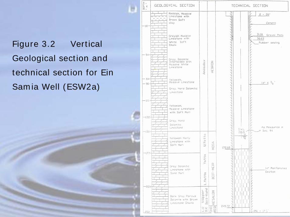
Geological borehole logs are mainly compiled on the basis
of rock samples (geotechnical assessments, oil and gas
exploration, … etc) (see Figure 3.2)
The logs normally consist of written descriptions of the
geology (lithological description of rock types) (see
Figure 3.2)
4/44/4
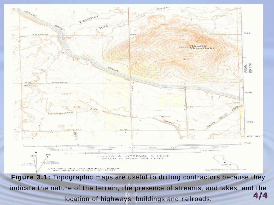
Figure 3.1: Topographic maps are useful to drilling contractors because they
indicate the nature of the terrain, the presence of streams, and lakes, and the
location of highways, buildings and railroads. 4/44/4
4/44/4
Figure 3.2 Vertical
Geological section and
technical section for Ein
Samia Well (ESW2a)

33 Desk Studies and Preliminary Field Desk Studies and Preliminary Field ReconnaissanceReconnaissance
Topographical area like rivers, wadi intersection and
coastal areas may indicate the presence of groundwater;
The slope of the terrain shown on the map usually
indicates the direction of shallow groundwater flow.
Geological borehole logs are mainly compiled on the basis
of rock samples (geotechnical assessments, oil and gas
exploration, … etc) (see Figure 3.2)
The logs normally consist of written descriptions of the
geology (lithological description of rock types) (see
Figure 3.2)
4/44/4
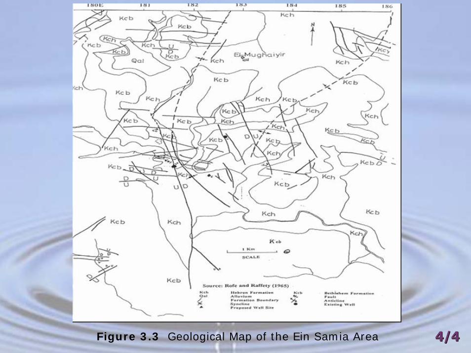
4/44/4Figure 3.3 Geological Map of the Ein Samia Area
33 Desk Studies and Preliminary Field Desk Studies and Preliminary Field ReconnaissanceReconnaissance
3.2 Hydrometeorological Methods
When precipitation over evaporation is large then the recharge
into the groundwater basin is large (that is when the geological
formations area sufficiently permeable)
4/44/4
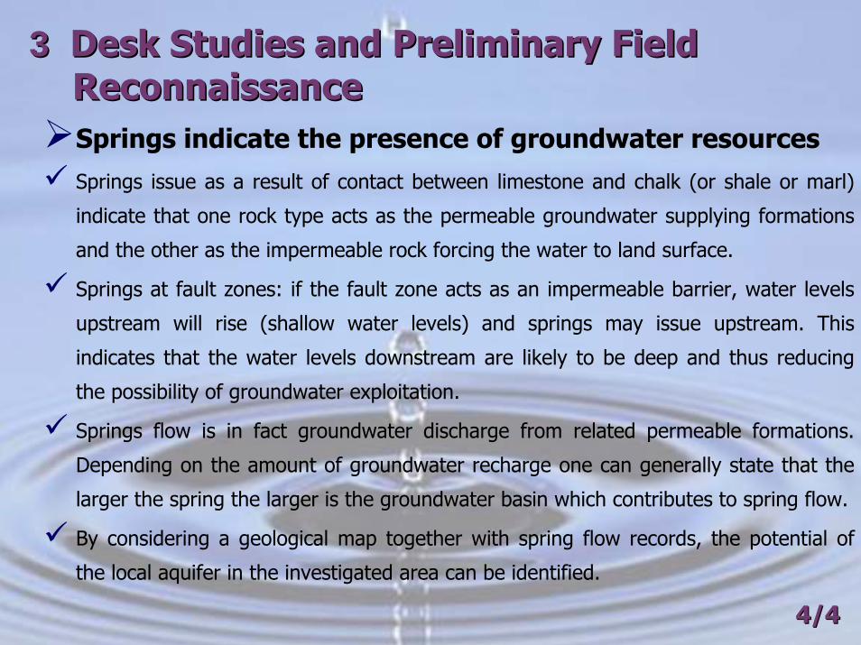
33 Desk Studies and Preliminary Field Desk Studies and Preliminary Field ReconnaissanceReconnaissanceSprings indicate the presence of groundwater resourcesSprings issue as a result of contact between limestone and chalk (or shale or marl)
indicate that one rock type acts as the permeable groundwater supplying formations
and the other as the impermeable rock forcing the water to land surface.
Springs at fault zones: if the fault zone acts as an impermeable barrier, water levels
upstream will rise (shallow water levels) and springs may issue upstream. This
indicates that the water levels downstream are likely to be deep and thus reducing
the possibility of groundwater exploitation.
Springs flow is in fact groundwater discharge from related permeable formations.
Depending on the amount of groundwater recharge one can generally state that the
larger the spring the larger is the groundwater basin which contributes to spring flow.
By considering a geological map together with spring flow records, the potential of
the local aquifer in the investigated area can be identified.
4/44/4

33 Desk Studies and Preliminary Field Desk Studies and Preliminary Field ReconnaissanceReconnaissanceWadis and Discharges
If the pattern of a wadi runoff is dense, then the permeability of the
(underneath) formations is low. Most of the precipitation will become
surface runoff thereby creating this dense pattern.
When the pattern is not very dense then the permeability of the
formation is high: much of the precipitation will infiltrate and there will
be hardly any surface runoff to create a dense pattern. Thus, these
wadis are major sources of groundwater pollution should the wadis
become contaminated
4/44/4
33 Desk Studies and Preliminary Field Desk Studies and Preliminary Field ReconnaissanceReconnaissance
3.3 Available Groundwater Data
Geophysical reports: identify sections with interpreted resistivities;
Well site reports: you may find geological logs, geophysical logs, water
sample analysis, well design, pumping test data, groundwater level records,
pumping rate data … etc;
Maps and sections;
Groundwater assessment reports;
4/44/4

33 Desk Studies and Preliminary Field Desk Studies and Preliminary Field ReconnaissanceReconnaissance
3.4 Satellite Imagery Studies
Satellites circling around the earth take pictures of the earth surface (see
Figure 3.4). The full light spectrum may be used when taking these
pictures or certain wave lengths of the spectrum may be selected.
Groundwater related features on satellite pictures can be detected by bare
eye and by using a stereoscope.
The best known picture are the LANDSAT images taken by satellites
launched by the USA and the SPOT images produced by satellites brought
into orbit by France.
4/44/4
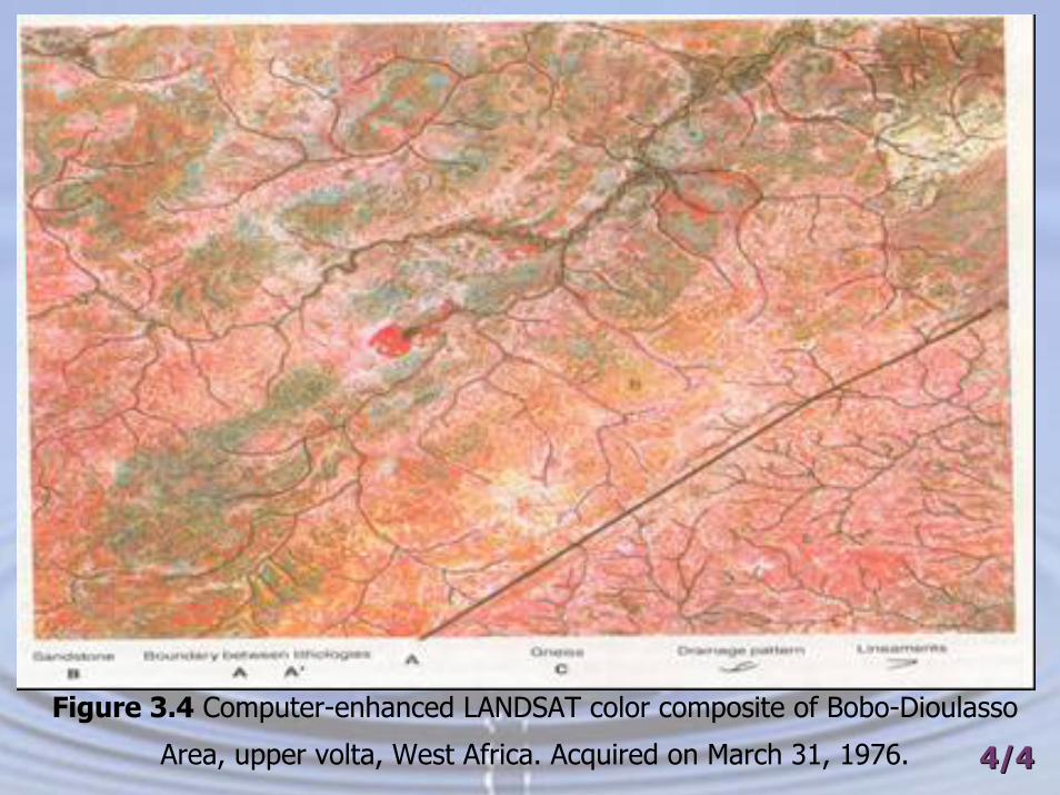
Figure 3.4 Computer-enhanced LANDSAT color composite of Bobo-Dioulasso
Area, upper volta, West Africa. Acquired on March 31, 1976. 4/44/4
33 Desk Studies and Preliminary Field Desk Studies and Preliminary Field ReconnaissanceReconnaissance
3.4 Satellite Imagery Studies
Interpretations
Satellite images are very handy tools to obtain a regional overview of
the geology.
The images can be used to get an impression on the regional drainage
system.
Combining the geological and surface water information, a
hydrogeological assessment of the “imaged area” can be made.
The images can be used to identify lineaments extending over several
tens or even hundreds of kilometers.
4/44/4
33 Desk Studies and Preliminary Field Desk Studies and Preliminary Field ReconnaissanceReconnaissance
3.5 Aerial Photography Analysis and Fracture Traces
Technique for Sitting a Well
General Notes
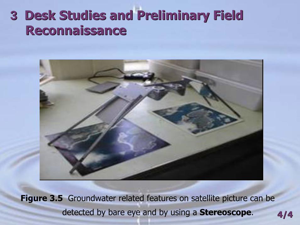
Aerial photos are taken from an aeroplane. The plane follows a flight
path covering completely the selected area. The photos taken are partly
overlapping each other in order to be able to obtain 3-dimensional view
with a stereoscope. The instrument consists of two sets of mirrors and
lenses which produce the three dimensional view (see Figure 3.5).
4/44/4
33 Desk Studies and Preliminary Field Desk Studies and Preliminary Field ReconnaissanceReconnaissance
Figure 3.5 Groundwater related features on satellite picture can be
detected by bare eye and by using a Stereoscope. 4/44/4
33 Desk Studies and Preliminary Field Desk Studies and Preliminary Field ReconnaissanceReconnaissance
3.5 Aerial Photography Analysis and Fracture Traces
Technique for Sitting a Well
Stratgraphical layering of consolidated sedimentary rocks can be
observed as ‘bands’ on the photos.
Shales, mudstones and siltstones can be recognized by ‘bands’ of
darkgrey to black tones.
Not very permeable carbonate rocks such as limestone and dolomites
can be identified by their massive banding and usually lighter tones.
Permeable limestones and dolomites are often identified by the
presence of karstic features including sinkholes (see Figure 3.6).
4/44/4

Figure 3.6 Effects of fissure density and orientation on the development of
caverns
33 Desk Studies and Preliminary Field Desk Studies and Preliminary Field ReconnaissanceReconnaissance
4/44/4
33 Desk Studies and Preliminary Field Desk Studies and Preliminary Field ReconnaissanceReconnaissance
River alluvial deposits (gravel, sands, clays and silt) can be recognized
from the presence of river terraces.
From above, the identified on the aerial photos can be classified as
aquifers, aquitards, … etc.
The type, location, and size of the aquifers present in the area give an
indication of the groundwater potential.
In the saddles and crests of large folds, fissures have often formed
as a result of lateral issues.
The presence of a spring is indicated by dense vegetation.
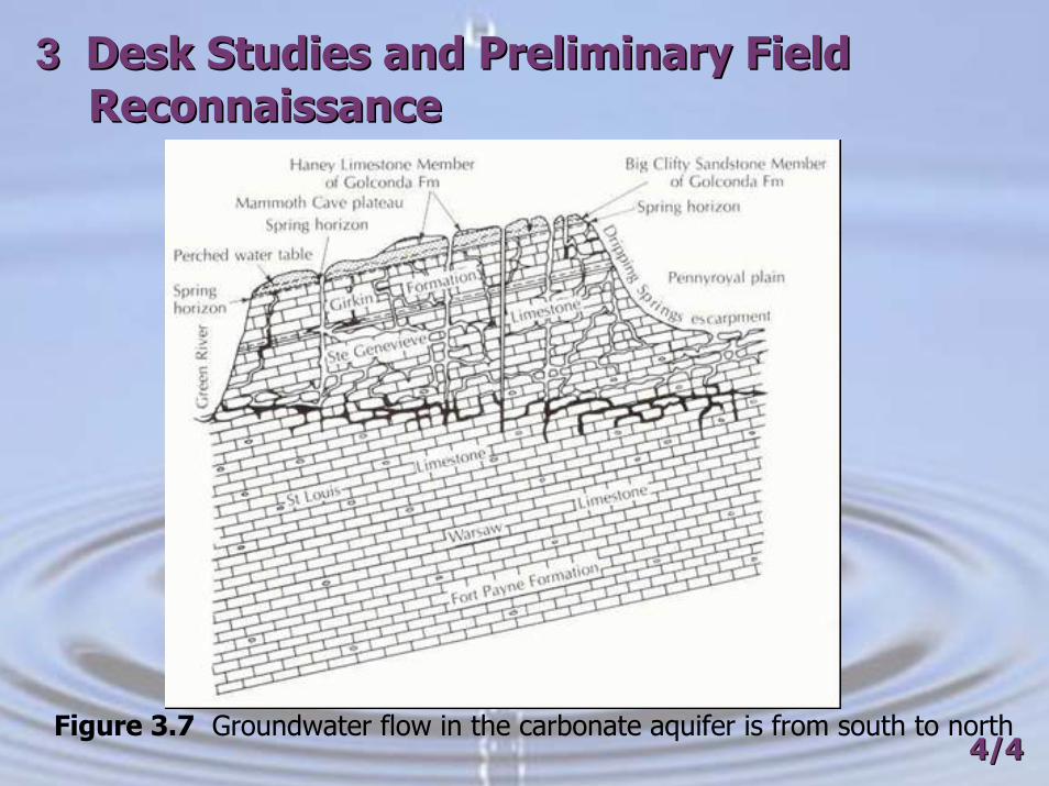
Groundwater is known to be concentrated in fracture zone found in
many different rock types ( see Figure 3.7).
4/44/4
33 Desk Studies and Preliminary Field Desk Studies and Preliminary Field ReconnaissanceReconnaissance
Figure 3.7 Groundwater flow in the carbonate aquifer is from south to north4/44/4
33 Desk Studies and Preliminary Field Desk Studies and Preliminary Field ReconnaissanceReconnaissance
In the identification of fracture traces on aerial photographs, a low
magnification stereoscope is generally used. (60% stereoscopic
overlapping, 1:20,000 scale. 20% overlapping between flight lines).
Possible fracture traces are indicated by drawing on the photograph.
One problem in identification is the confusion of linear features of human
origin (fences, roads, … etc.) with natural linear feature. Following the
mapping of linear features on air photos, it is necessary to make a field
check.
4/44/4
33 Desk Studies and Preliminary Field Desk Studies and Preliminary Field ReconnaissanceReconnaissance
In crystalline rock areas, high-yield wells are generally
associated with fracture traces which may not be necessarily
correspond to topographic lows.
A zig-zag offsets in the regional valley alignment assure well
developed fracture traces.
Openings in the fault zones and at the weathered parts of joint
systems may indicate exploitable groundwater resources.
4/44/4
Fracture Traces and LineamentsFracture Traces and Lineaments
Fracture traces are located by study of linear features on aerial or
satellite photographs.
Natural linear features from 300 m to around 1500 m in length are
fracture traces.
Natural linear features greater than 1500 m in length are termed
lineaments. Some lineaments are up to 150 km long.
Fracture traces are surface expressions of joints, zone of joint
concentration or faults.
4/44/4

Fracture Traces and LineamentsFracture Traces and Lineaments
On air photos, natural linear features consist tonal variation in soils:
Alignment of vegetation patterns;
Straight stream segments or valleys;
Aligned surface depressions;
Gaps in ridges;
It is generally believed that the joint sets tend to be perpendicular. They
are known to extend to a depth of 1000 m at one Arizona location as an
example (see Figure 3.8).
4/44/4
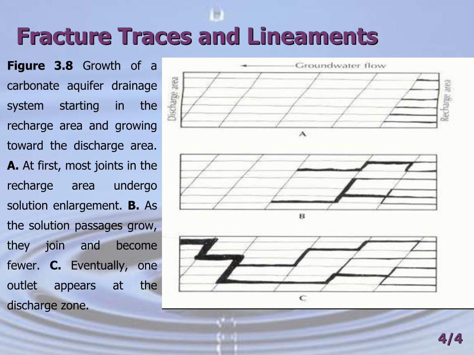
Fracture Traces and LineamentsFracture Traces and LineamentsFigure 3.8 Growth of a
carbonate aquifer drainage
system starting in the
recharge area and growing
toward the discharge area.
A. At first, most joints in the
recharge area undergo
solution enlargement. B. As
the solution passages grow,
they join and become
fewer. C. Eventually, one
outlet appears at the
discharge zone.
4/44/4
Fracture Traces and LineamentsFracture Traces and LineamentsFracture zones are less resistant to erosion. Hence, valley and stream
segments tend to run along fracture zone.
Fracture traces and lineaments appear to have their greatest utility in
rocks where secondary permeability and porosity dominate and where
intergranular characteristics combine with secondary openings influencing
weathering and soil water and groundwater movement. Fracture traces and
lineaments are considered surface manifestations of vertical to near-vertical
zone of fracture concentration.
Fracture traces may be related to regional tectonic activity. They tend to
be oriented at a constant angle to the regional structural trend. However, the
orientation appears to be independent of local folds.
Fracture traces in carbonate rocks are typically areas of solution. Aligned
sinkhole or surface sags are typical surface expressions (see Figure 3.9).4/44/4
Fracture Traces and LineamentsFracture Traces and Lineaments
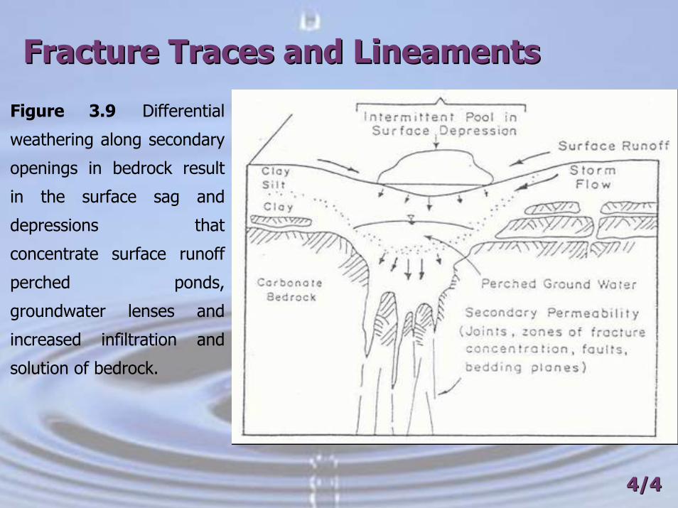
Figure 3.9 Differential
weathering along secondary
openings in bedrock result
in the surface sag and
depressions that
concentrate surface runoff
perched ponds,
groundwater lenses and
increased infiltration and
solution of bedrock.
4/44/4

Fracture Traces and LineamentsFracture Traces and LineamentsLineaments are known to cut across rocks of many ages and cross folds and
faults (see Figure 3.10).
4/44/4
Figure 3.10 Lineaments and
fractures map of Ein Samia

Fracture Traces and LineamentsFracture Traces and Lineaments
Lineaments have been observed to be parallel to the major joint sets in
flat-lying or gently dipping strata, but this is not the case if the strata are
steeply dipping.
If surface area separated by major faults, the individual fault blocks may
have fracture traces of different orientation.
The majority of fracture traces control is evident have been described as
having a “stair-step” pattern.
4/44/4

Fracture Traces and LineamentsFracture Traces and Lineaments
Statistical studies of wells in carbonate terrane have shown that those
located on fracture traces, either intentionally or accidentally have a
greater yield than those not on fracture traces.
Fracture traces are known to reveal narrow zones (2 to 20 m wide)
suitable for groundwater prospecting, high permeability and porosity
avenues 10 to 1000 times that of adjacent strata.
Caliper logs of wells on fracture traces in carbonate-rock terrane showed
many more cavernous opening and enlarged bedding planes than logs of
those wells drilled in interfracture areas (see Figure 3.11).
4/44/4
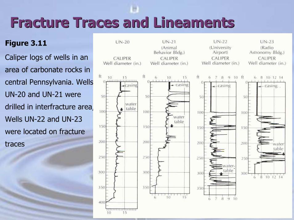
Fracture Traces and LineamentsFracture Traces and LineamentsFigure 3.11
Caliper logs of wells in an
area of carbonate rocks in
central Pennsylvania. Wells
UN-20 and UN-21 were
drilled in interfracture area,
Wells UN-22 and UN-23
were located on fracture
traces
4/44/4
Fracture Traces and LineamentsFracture Traces and Lineaments
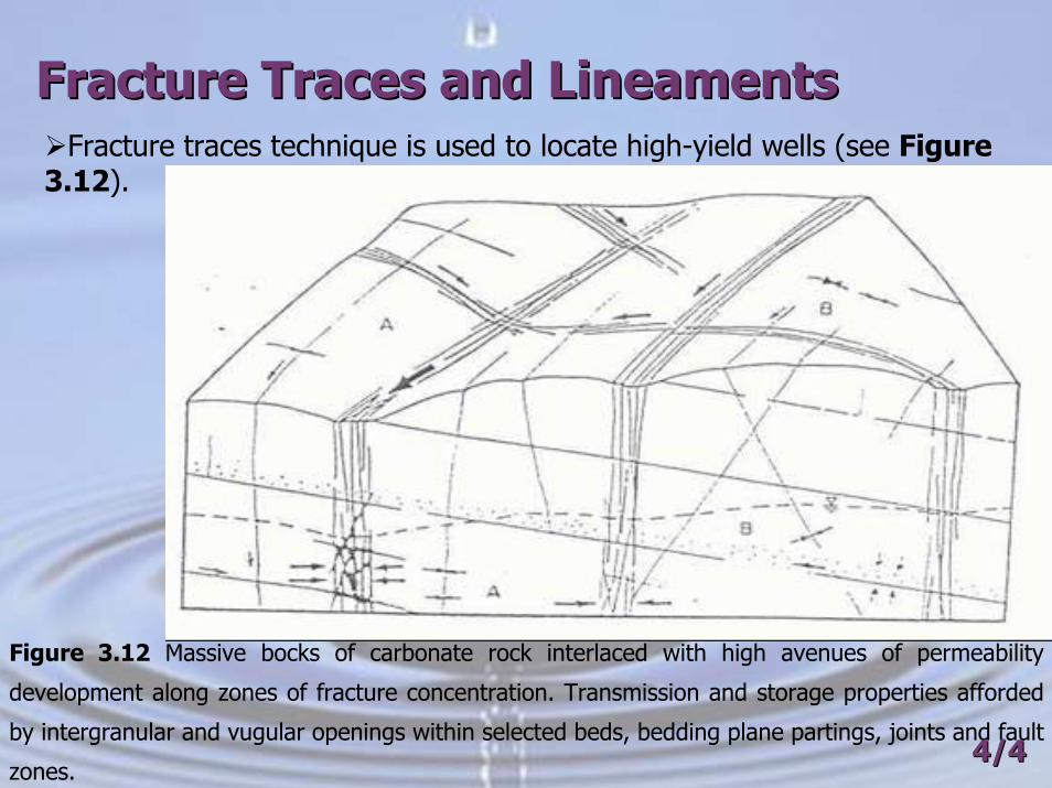
Figure 3.12 Massive bocks of carbonate rock interlaced with high avenues of permeability
development along zones of fracture concentration. Transmission and storage properties afforded
by intergranular and vugular openings within selected beds, bedding plane partings, joints and fault
zones. 4/44/4
Fracture traces technique is used to locate high-yield wells (see Figure 3.12).

Fracture Traces and LineamentsFracture Traces and Lineaments
The problems with lineaments and fracture traces:
What are the depth and width of lineaments and fracture traces!!;
Accurate location on the ground!;
Well yield depends also on well radius, well depth and diameter,
casing length, method of drilling, degree of well development, depth to
water table, presence of various changes of rock type, dip of beds,
topographical settings, rock type, type of fold structure, presence and
type of joints, number and type of zones of fracture concentration, …
etc.;
If fracture traces are absent from a property on which water is
required, the use of expert advice would not help except to point out
the increased risk of obtaining a low yield. 4/44/4
Well SittingWell Sitting
Well sitting is important prior to any water resources development
project.
Site studies are necessary prior to construction of projects as sanitary
landfills, land-treatment systems for wastewater, surface mines, power
plants, artificial-recharge lagoons, nuclear-waste repositories, dams and
reservoirs.
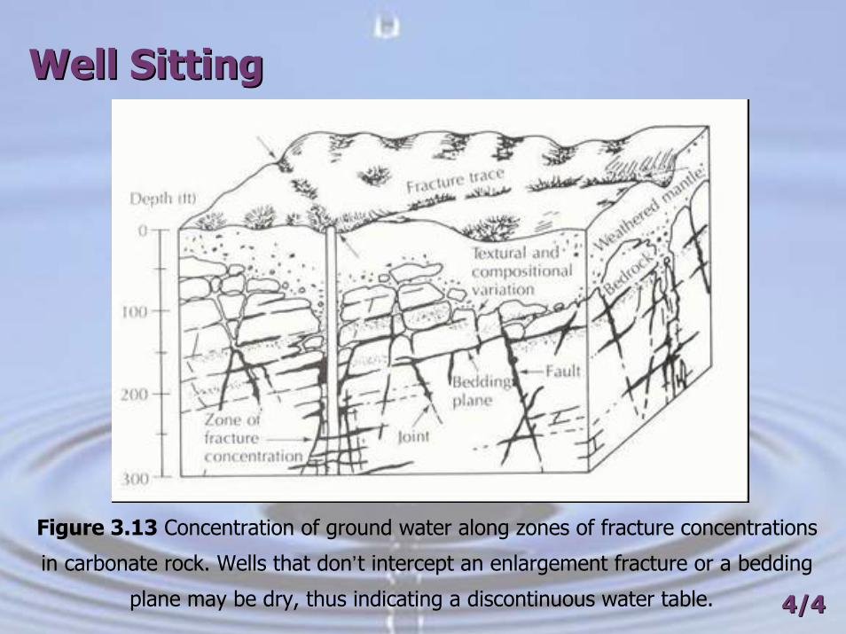
The greatest yields come from wells located at the intersection of two
fracture traces or more (see Figure 3.13).
4/44/4
Well SittingWell Sitting
Figure 3.13 Concentration of ground water along zones of fracture concentrations
in carbonate rock. Wells that don’t intercept an enlargement fracture or a bedding
plane may be dry, thus indicating a discontinuous water table. 4/44/4
Well SittingWell Sitting
Some investigations failed to correlate high well yields and well locations
with respect to fracture traces sites in carbonate rocks because:
Fracture traces were not mapped correctly;
The width of influence of fracture trace was not known;
Wells did not hit the center lines of fracture traces;
4/44/4

Well SittingWell SittingSome variability in yield remains for wells located on lineaments due to the
fact that joints, fractures, bedding plane partings and secondary weathering
is not equally well developed beneath lineaments and an element of chance
and variability of penetrating openings will always remain when drilling on
fracture concentration. Variable fracture development has been observed in
cross-sectional views.
The same variability of fracture and joint development beneath lineaments
has not been documented but it is recommend that all lineament well sites
also located on fracture trace intersections or on single fracture traces to
increase the probability of penetrating the maximum number of secondary
openings.
4/44/4
Well SittingWell Sitting
Fracture-trace analysis is also very useful in determining the locations of
groundwater monitoring wells. Because groundwater flow preferentially
follows the most permeable pathway, monitoring wells should be located
on fracture traces.
It should be noted that wells located in valley bottom settings show
higher yields than wells located on adjacent uplands (see Figure 3.14).
4/44/4
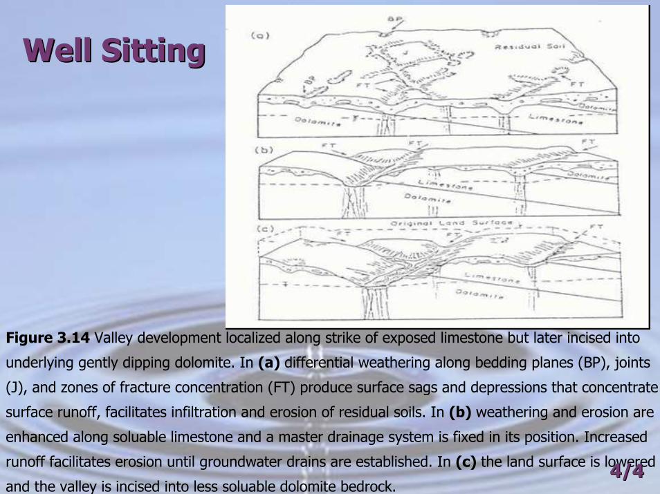
Figure 3.14 Valley development localized along strike of exposed limestone but later incised into
underlying gently dipping dolomite. In (a) differential weathering along bedding planes (BP), joints
(J), and zones of fracture concentration (FT) produce surface sags and depressions that concentrate
surface runoff, facilitates infiltration and erosion of residual soils. In (b) weathering and erosion are
enhanced along soluable limestone and a master drainage system is fixed in its position. Increased
runoff facilitates erosion until groundwater drains are established. In (c) the land surface is lowered
and the valley is incised into less soluable dolomite bedrock.
Well SittingWell Sitting
4/44/4
Well SittingWell Sitting
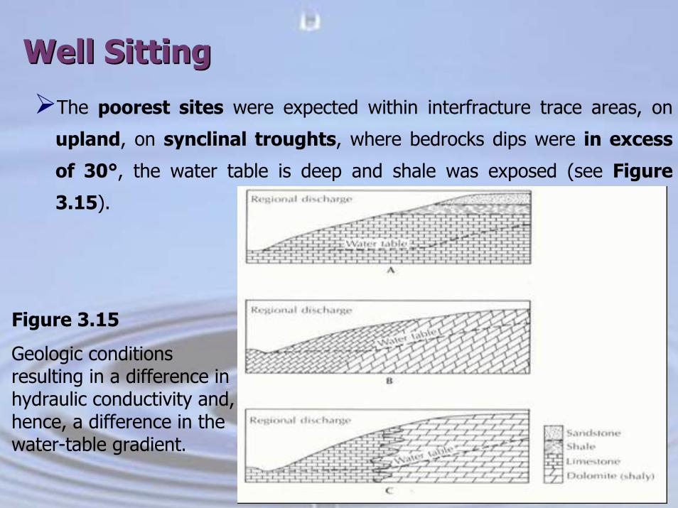
The poorest sites were expected within interfracture trace areas, on
upland, on synclinal troughts, where bedrocks dips were in excess
of 30°, the water table is deep and shale was exposed (see Figure
3.15).
4/44/4
Figure 3.15
Geologic conditions resulting in a difference in hydraulic conductivity and, hence, a difference in the water-table gradient.
Choosing a Well SiteChoosing a Well Site
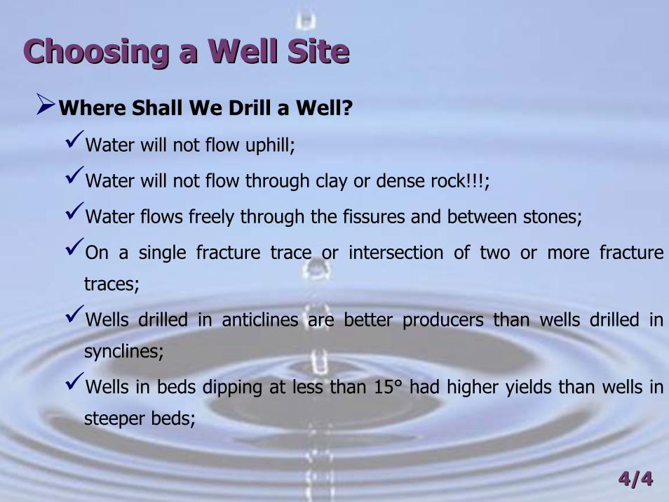
Where Shall We Drill a Well?
Water will not flow uphill;
Water will not flow through clay or dense rock!!!;
Water flows freely through the fissures and between stones;
On a single fracture trace or intersection of two or more fracture
traces;
Wells drilled in anticlines are better producers than wells drilled in
synclines;
Wells in beds dipping at less than 15° had higher yields than wells in
steeper beds;
4/44/4

Choosing a Well SiteChoosing a Well Site
What other considerations should be taken in sitting a
well.
Your choice of well site will affect the safety and performance of your well.
As you examine various sites, remember to consider any future development
plans for your farm or acreage such as barns, storage sheds and bulk fuel
tanks. You must also consider provincial regulations that dictate well location.
Most contaminants enter the well either through the top or around the
outside of the casing. Sewage or other contaminants may percolate down
through the upper layers of the ground surface to the aquifer. The following
criteria are intended to prevent possible contamination of your well and the
aquifer. It is both your and the driller’s responsibility to ensure that: 4/44/4
Choosing a Well SiteChoosing a Well SiteThe well is accessible for cleaning, testing, monitoring, maintenance and
repair;
The ground surrounding the well is sloped away from the well to prevent
any surface run off from collecting or ponding;
The well is up-slope and as far as possible from potential contamination
sources such as septic systems, barnyards or surface water bodies;
The well is not housed in any building other than a bona fide pumphouse.
The pumphouse must be properly vented to the outside to prevent any
buildup of dangerous naturally occurring gases
The well is not located in a well pit.
4/44/4
Choosing a Well SiteChoosing a Well Site
Minimum distance requirements.
Provincial regulations outline minimum distance requirements as follows.
Equivalent imperial distances in feet are rounded up to nearest foot. The
well must be:
10 m (33 ft.) from a watertight septic tank;
15 m (50 ft.) from a sub-surface weeping tile effluent disposal field or
evaporation mound;
50 m (165 ft.) from sewage effluent discharge to the ground;
100 m (329 ft.) from a sewage lagoon;
50 m (165 ft.) from above-ground fuel storage tanks;
3.25 m (11 ft.) from existing buildings;
4/44/4
Choosing a Well SiteChoosing a Well SiteMinimum distance requirements.
2 m (7 ft.) from overhead power lines if: the line conductors are
insulated or weatherproofed and the line is operated at 750 volts or less;
6 m (20 ft.) from overhead power lines if the well: does not have a pipe
and sucker rod pumping system has a PVC or non-conducting pipe
pumping system has well casing sections no greater than 7 m (23 ft.) in
length;
12 m (40 ft.) from overhead power lines for all other well constructions;
500 m (1,641 ft.) from a sanitary landfill, modified sanitary landfill or dry
waste site.
4/44/4

3 Desk Studies and Preliminary Field 3 Desk Studies and Preliminary Field ReconnaissanceReconnaissance
3.6 Hydrogeological Mapping and Well inventories
Hydrogeological mapping is the study of rock types and drainage
conditions in the field with emphasis on hydrogeological aspects (see
Figure 3.16);
4/44/4

3 Desk Studies and Preliminary Field 3 Desk Studies and Preliminary Field ReconnaissanceReconnaissance
Stratigraphic section of the West Bank
4/44/4

Northern West Bank cross section
3 Desk Studies and Preliminary Field 3 Desk Studies and Preliminary Field ReconnaissanceReconnaissance
4/44/4
Figure 3.16
Hydrogeological
Map of the West
BankSouthern West Bank cross section
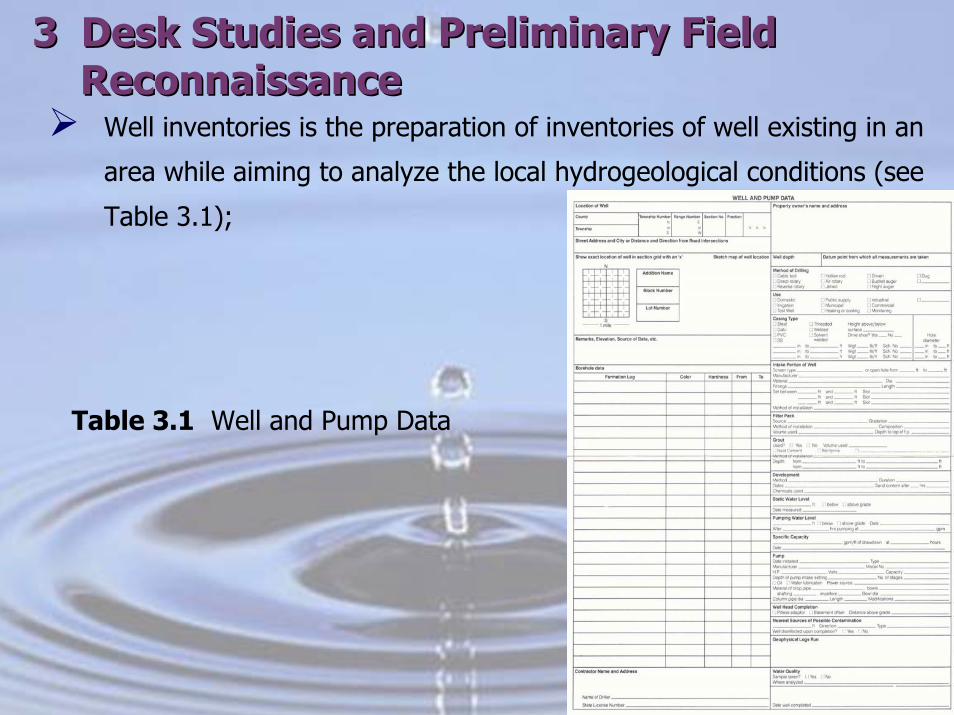
Well inventories is the preparation of inventories of well existing in an
area while aiming to analyze the local hydrogeological conditions (see
Table 3.1);
Table 3.1 Well and Pump Data
3 Desk Studies and Preliminary Field 3 Desk Studies and Preliminary Field ReconnaissanceReconnaissance
4/44/4
3 Desk Studies and Preliminary Field 3 Desk Studies and Preliminary Field ReconnaissanceReconnaissance
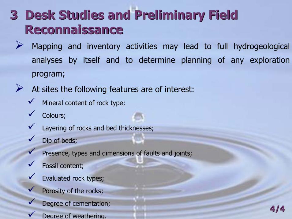
Mapping and inventory activities may lead to full hydrogeological
analyses by itself and to determine planning of any exploration
program;
At sites the following features are of interest:
Mineral content of rock type;
Colours;
Layering of rocks and bed thicknesses;
Dip of beds;
Presence, types and dimensions of faults and joints;
Fossil content;
Evaluated rock types;
Porosity of the rocks;
Degree of cementation;
Degree of weathering.4/44/4
3 Desk Studies and Preliminary Field 3 Desk Studies and Preliminary Field ReconnaissanceReconnaissance
Well inventories cover all type of wells, production, monitoring,
abandoned, exploration, … etc.
Table 3.2 shows the index for Model
Map
Table 3.2 Index for the Model Map
4/44/4

3 Desk Studies and Preliminary Field 3 Desk Studies and Preliminary Field ReconnaissanceReconnaissance
Table 3.2 Index for the Model Map
4/44/4

SESSION 9SESSION 9
GROUNDWATER EXPLORATIONGROUNDWATER EXPLORATIONIIII
Dr Amjad AliewiDr Amjad Aliewi
House of Water and Environment
Email: [email protected] , Website: www.hwe.org.ps
44 Surface Geophysical TechniquesSurface Geophysical Techniques
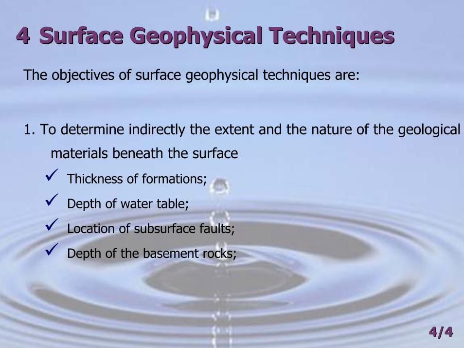
The objectives of surface geophysical techniques are:
1. To determine indirectly the extent and the nature of the geological
materials beneath the surface
Thickness of formations;
Depth of water table;
Location of subsurface faults;
Depth of the basement rocks;
4/44/4
44 Surface Geophysical TechniquesSurface Geophysical Techniques
2. To minimize the extent and thickness of fresh
groundwater lenses in saline aquifer (water quality) or clay
lenses in aquifers (lithology).
The correlation of geophysical data with well logs or test-boring data
is generally more reliable than either type of information used by
itself. The interpretation of physical parameters into rock type
requires information from remote sensing surveys, mapping and, in
particular, data from exploration drilling activities.
4/44/4
44 Surface Geophysical TechniquesSurface Geophysical Techniques
In geophysical techniques, rock parameters are measured as a
response to energy fluxes injected into the earth. The most common
geophysical techniques are:
Geo-electrical;
Electromagnetic;
Seismic;
4/44/4

44 Surface Geophysical TechniquesSurface Geophysical Techniques4.1 Surface Geo-electrical Techniques (Electrical
Resistivity)
4.1.1 Working Principle
These techniques are based on the injection of an electrical current of very low
frequency into the earth by means of two current electrodes (Figure 4.1);
The potential differences which are created between these electrodes are
measured at another pair of intermediate electrodes, the measuring or potential
electrodes;
Readings of current strength at the current electrodes, and potential differences
at the measuring electrodes, and potential differences at the measuring electrodes
enable us to determine rock resistivities;
These resistivities can be related to subsurface rock types, rock water contents
and groundwater quality (pore water resistivity). This information can be used to
identify permeable rocks. 4/44/4

44 Surface Geophysical TechniquesSurface Geophysical Techniques
Figure 4.1 Set up for a geo-electrical measurement 4/44/4
44 Surface Geophysical TechniquesSurface Geophysical Techniques
4.1.2 The Concept of Apparent Resistivity
When carrying out a geo-electrical measurement we do not measure the
resistivities of the individual layers, but we are able to compute a so-called
apparent resistivity. The apparent resistivity is in fact a combination of the
resistivities of the individual layers (see Figure 4.2);
4/44/4
44 Surface Geophysical TechniquesSurface Geophysical Techniques
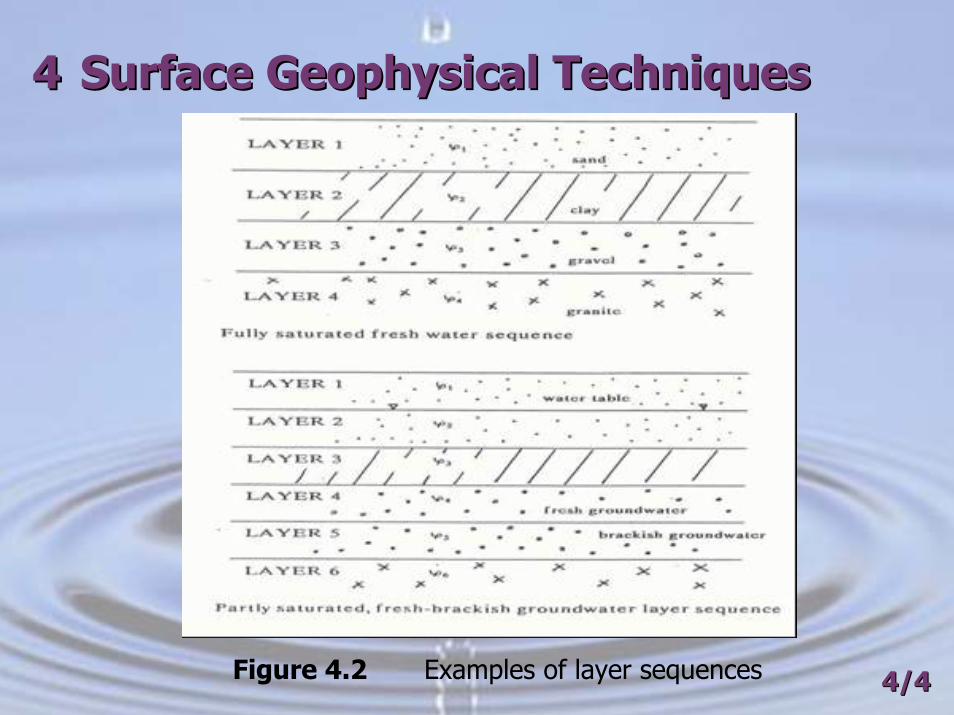
Figure 4.2 Examples of layer sequences 4/44/4

44 Surface Geophysical TechniquesSurface Geophysical TechniquesThe general formulation of Ohm’s law is as follows:
-dV=IxR (1)
Where,
dV potential drop (volt/m)
I current length (Ampere)
R resistance (ohm)
Imagine a single current source at land surface. Assume that the resistivities of
the individual rock layers can be combined in apparent resistivities. The current (I)
injected at the current sources expands itself as a semi sphere into the earth, with
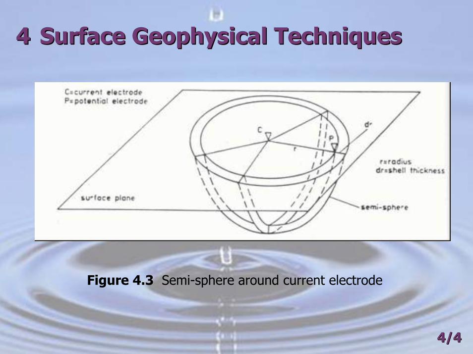
the atmosphere acting as a complete insulator. Figure 4.3 shows that around the
source semi-spherical shells can be considered through which the current is
passing at right angles.4/44/4
44 Surface Geophysical TechniquesSurface Geophysical Techniques
Figure 4.3 Semi-sphere around current electrode
4/44/4

44 Surface Geophysical TechniquesSurface Geophysical TechniquesConsider such a semi-spherical shell located at a given distance from the
current source. If we consider equation 1 for the shell then the resistance
(R) is proportional to the width of this shell and it is inversely proportional
to the cross sectional area. The resistance is also proportional to the
apparent resistivity of the medium. Thus, we can write:
(2)
Where,
φa apparent resistivity (Ω-m)
dr width of shell (m)
r distance from shell to current source (m)4/44/4
22 rdrxR a π
ϕ=
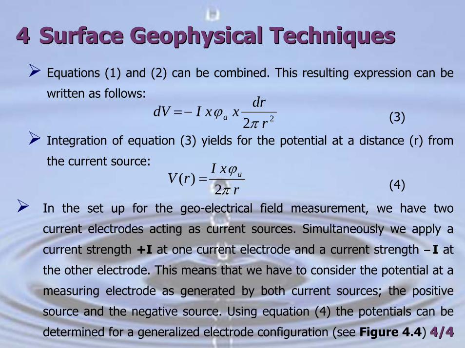
44 Surface Geophysical TechniquesSurface Geophysical TechniquesEquations (1) and (2) can be combined. This resulting expression can be
written as follows:
(3)
Integration of equation (3) yields for the potential at a distance (r) from
the current source:
(4)
In the set up for the geo-electrical field measurement, we have two
current electrodes acting as current sources. Simultaneously we apply a
current strength +I at one current electrode and a current strength –I at
the other electrode. This means that we have to consider the potential at a
measuring electrode as generated by both current sources; the positive
source and the negative source. Using equation (4) the potentials can be
determined for a generalized electrode configuration (see Figure 4.4) 4/44/4
22 rdrxxIdV a π
ϕ−=
rxI
rV a
πϕ
2)( =

44 Surface Geophysical TechniquesSurface Geophysical Techniques
Figure 4.4 Generalized layout for a measurement
4/44/4
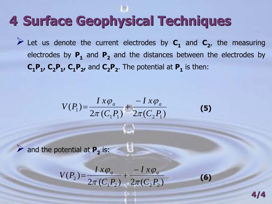
44 Surface Geophysical TechniquesSurface Geophysical TechniquesLet us denote the current electrodes by C1 and C2, the measuring
electrodes by P1 and P2 and the distances between the electrodes by
C1P1, C2P1, C1P2, and C2P2. The potential at P1 is then:
(5)
and the potential at P2 is:
(6)
4/44/4
)(2)(2)(
12111 PC
xIPC
xIPV aa
πϕ
πϕ −
+=
)(2)(2)(
22212 PC
xIPC
xIPV aa
πϕ
πϕ −
+=
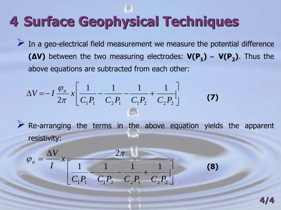
44 Surface Geophysical TechniquesSurface Geophysical TechniquesIn a geo-electrical field measurement we measure the potential difference
(∆V) between the two measuring electrodes: V(P1) – V(P2). Thus the
above equations are subtracted from each other:
(7)
Re-arranging the terms in the above equation yields the apparent
resistivity:
(8)
4/44/4
⎥⎦
⎤⎢⎣
⎡+−−−=∆
22211211
11112 PCPCPCPC
xIV a
πϕ
⎥⎦
⎤⎢⎣
⎡+−−
∆=
22122111
11112
PCPCPCPC
xIV
aπϕ

44 Surface Geophysical TechniquesSurface Geophysical Techniques
The most commonly used electrode layouts are the ‘Wenner’ (see
Figure 4.5) and ‘Schlumberger’ configurations (see Figure 4.6).
Wenner configuration is symmetrical with the four electrodes always
at equal distances from each other. The Schlumberger configuration is
also symmetrical, but the distance between the measuring electrodes
differs from the spacing between the measuring and current
electrodes.
Figure 4.5
Wenner layout
4/44/4
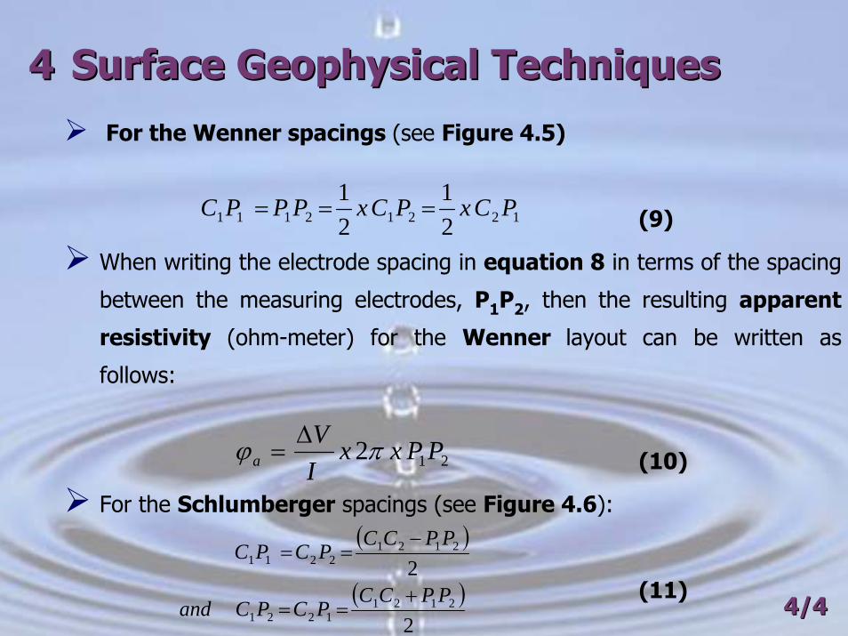
44 Surface Geophysical TechniquesSurface Geophysical TechniquesFor the Wenner spacings (see Figure 4.5)
(9)
When writing the electrode spacing in equation 8 in terms of the spacing
between the measuring electrodes, P1P2, then the resulting apparent
resistivity (ohm-meter) for the Wenner layout can be written as
follows:
(10)
For the Schlumberger spacings (see Figure 4.6):
(11)4/44/4
12212111 21
21 PCxPCxPPPC ===
212 PPxxIV
a πϕ ∆=
( )
( )2
22121
1221
21212211
PPCCPCPCand
PPCCPCPC
+==
−==
44 Surface Geophysical TechniquesSurface Geophysical Techniques
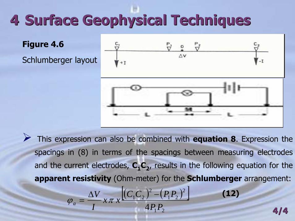
Figure 4.6
Schlumberger layout
This expression can also be combined with equation 8. Expression the
spacings in (8) in terms of the spacings between measuring electrodes
and the current electrodes, C1C2, results in the following equation for the
apparent resistivity (Ohm-meter) for the Schlumberger arrangement:
(12)
4/44/4
( ) ( )[ ]21
221
221
4 PPPPCC
xxIV
a−∆
= πϕ

44 Surface Geophysical TechniquesSurface Geophysical Techniques
4.1.3 The Variable Electrode Distance Technique
During measurement, the distances between the current and
measuring electrodes are gradually increased, while the center
of the layout remains at a fixed point. Various current strength
and potential difference readings are taken at one location.
Apparent resistivities computed from current strength and
potential difference readings can be translated into resistivities
and thicknesses of individual subsurface layers.
4/44/4
44 Surface Geophysical TechniquesSurface Geophysical Techniques4.1.4 Field Guidelines
Select the area for geoelectrical surveying using the variable electrode
distance technique on the basis of all existing data available (remote
sensing; hydrogeological mapping and well inventories).
Geo-electrical techniques are used in areas of varying geologic nature.
The technique is also engaged in areas of varying geological nature. The
technique is also engaged in areas with consolidated sedimentary rock and
in the weathered parts of metamorphic and igneous rocks. The method
works best when we have:
Simple stratigraphical and tectonic conditions;
Moderate or no dip of the rock layers;
Large resistivity contrasts between subsurface layers4/44/4
44 Surface Geophysical TechniquesSurface Geophysical Techniques
Plot the measurements on section lines which are perpendicular to the
main strike direction of the subsurface rock layers. The distance between
section lines, and between the individual measurements depends on the
required amount of detail. Distances between measurements are 50-
1000 m.
4/44/4
44 Surface Geophysical TechniquesSurface Geophysical TechniquesExtend the electrode spacing along a straight line perpendicular to the
selected section lines. I and ∆V are measured from each electrode spacing,
while the center of the measurement line (the axes through the electrodes)
remains at a fixed position. At small electrode spacing the depth
penetration of the electrical current is small and the potential difference
readings relate to the resistivity of the first rock layer. When we proceed,
the readings at larger spacings relate to the deeper layers. We will
continue until the maximum electrode spacing is reached (as a “rule of
thumb” we can take that the maximum spacing between current
electrodes is equal to (3-4) times the required investigation depth).
However, the final decision on the completion of the measurements should
be taken in the field itself and depends on the shape of the (apparent)
resistivity curve and on the smoothness of this curve (only smooth curves
lend themselves to interpretation). 4/44/4
44 Surface Geophysical TechniquesSurface Geophysical Techniques
Selection of layout: In the Wenner set-up the electrode spacing C1P1,
P1P2, and P2C2 remain constant, but this also implies that after each
reading all four electrodes have to be brought to new, larger spaced
positions. In the Schlumberger arrangement the electrode spacings C1P1,
C2P2 are identical but differ from P1P2. During the measurement the P1P2 is
kept constant during a series of readings for increasing current electrode
spacing. Then the P1P2 is increased and again kept constant while the next
set of readings for increasing current electrode distances C1C2 is taken. On
the field curve we can distinguish the various sets of readings for typical
P1P2 values as “branches” which partly overlap each other.
4/44/4
44 Surface Geophysical TechniquesSurface Geophysical Techniques
In Wenner surveys ∆V can usually be measured somewhat more
accurate than in Schlumberger surveys where P1P2 is relatively small as
compared to the current electrode spacing. The Schlumberger set up has
as its main advantage that lateral changes in the subsurface geology can
better be detected from shifts in the various field curve branches. The
interpretation of Schlumberger field curves with curve matching techniques
is also more accurate. Wenner surveys may be somewhat faster than the
Schlumberger surveys, but the Wenner survey usually requires one or
more laborer to replace the electrodes.
4/44/4
44 Surface Geophysical TechniquesSurface Geophysical Techniques
Taking the measurements: select the electrode spacings in such a way
that half the current electrode spacing, C1C2/2, plot more or less
equidistantly on double-logarithmic paper. Measuring tapes may be rolled
out to mark the sites for the electrodes or marks may be made on the
cables. During the measurement, determine the apparent resistivity for
each electrode spacing from the recorded I and ∆V (or their ratio).
Multiply ∆V/I with a geometrical factor G (equal to that part of equation
10 or 12 describing the electrode spacings) will give us the value for the
apparent resistivity.
4/44/4

44 Surface Geophysical TechniquesSurface Geophysical Techniques
Plot the φa values for the production of a field curve straightaway on
log-log paper. φa values are usually plotted along the y-axes and the
corresponding C1C2/2 along the x-axes. Direct plotting helps identifying
errors become in the field, and not later in the office. An example of a
typical Schlumberger configuration is presented in Table 4.1
4/44/4

44 Surface Geophysical TechniquesSurface Geophysical Techniques
Table 4.1 Example of a typical Schlumberger configuration
GC1C2/2P1P2/2GC1C2/2P1P2/2
82.812623537754986715543145899421374247338865616
25304050607510075100125150200250300
1010101010101025252525252525
6.2818.849.511220031345170655.782151239347
1.52.54681012151215202530
0.50.50.50.50.50.50.50.544444
4/44/4
44 Surface Geophysical TechniquesSurface Geophysical Techniques
4.1.5 Principles of Resistivity Interpretation
In the field we measure I and ∆V for various electrode spacings. Then
apparent resistivity values are computed using equations 11 and 12. We
end up with a whole series of apparent resistivities for a range of electrode
spacings. The next step is to translate the values of apparent resistivity into
layer resistivities φ1 , φ2 ,φ3 etc. and into layer thicknesses h1, h2, h3 etc.
This interpretation is done by means of curve matching techniques which
are valid for horizontally stratified earth layers. Field curves showing
apparent resistivities against current electrode spacings are matched with
master curves which are computed from mathematical expressions. In case
field and master curves fit, the layer resistivities thickness at a measurement
location are similar to those used for the computation of the master curves.4/44/4
44 Surface Geophysical TechniquesSurface Geophysical Techniques
Traditionally sets of master curves which were determined from the
mathematical expressions were drawn on paper, and curve matching with
field curves was done manually. Nowadays the computation and
presentation of ‘master’ curves, and the storage and presentation of the
field curves is largely done on the personal computer.
Mathematical Expressions: for the case of two layers the final result
of the derivation for the mathematical expression will be presented. The
equation relates apparent resistivities to resistivities of the first and second
layer, the thickness of the first layer, and to current electrode spacings.
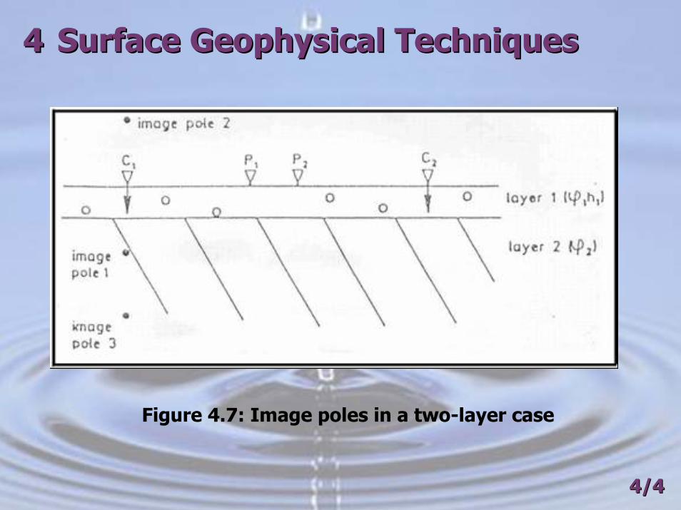
The deepest layer, which in case is the second layer, is always assumed to
be of infinite thickness (see Figure 4.7). Also, note that an electrode
configuration following the Schlumberger arrangement has been assumed.
The expression with a written on the left hand side in equation 13. 4/44/4
44 Surface Geophysical TechniquesSurface Geophysical Techniques
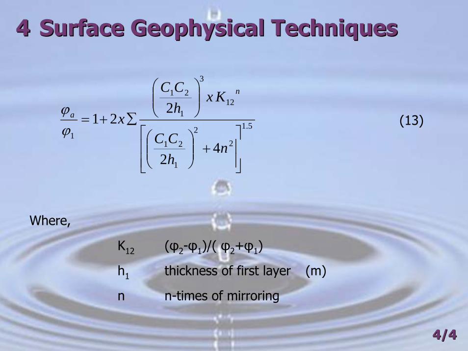
(13)
Where,
K12 (φ2-φ1)/( φ2+φ1)
h1 thickness of first layer (m)
n n-times of mirroring
4/44/4
5.1
22
1
21
12
3
1
21
1
42
221
⎥⎥⎦
⎤
⎢⎢⎣
⎡+⎟⎟
⎠
⎞⎜⎜⎝
⎛
⎟⎟⎠
⎞⎜⎜⎝
⎛
∑+=
nhCC
KxhCC
x
n
a
ϕϕ
44 Surface Geophysical TechniquesSurface Geophysical Techniques
Figure 4.7: Image poles in a two-layer case
4/44/4
44 Surface Geophysical TechniquesSurface Geophysical Techniques
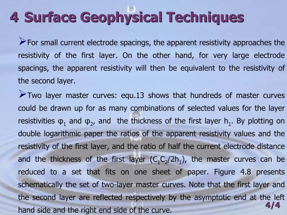
For small current electrode spacings, the apparent resistivity approaches the
resistivity of the first layer. On the other hand, for very large electrode
spacings, the apparent resistivity will then be equivalent to the resistivity of
the second layer.
Two layer master curves: equ.13 shows that hundreds of master curves
could be drawn up for as many combinations of selected values for the layer
resistivities φ1 and φ2, and the thickness of the first layer h1. By plotting on
double logarithmic paper the ratios of the apparent resistivity values and the
resistivity of the first layer, and the ratio of half the current electrode distance
and the thickness of the first layer (C1C2/2h1), the master curves can be
reduced to a set that fits on one sheet of paper. Figure 4.8 presents
schematically the set of two-layer master curves. Note that the first layer and
the second layer are reflected respectively by the asymptotic end at the left
hand side and the right end side of the curve.4/44/4
44 Surface Geophysical TechniquesSurface Geophysical Techniques
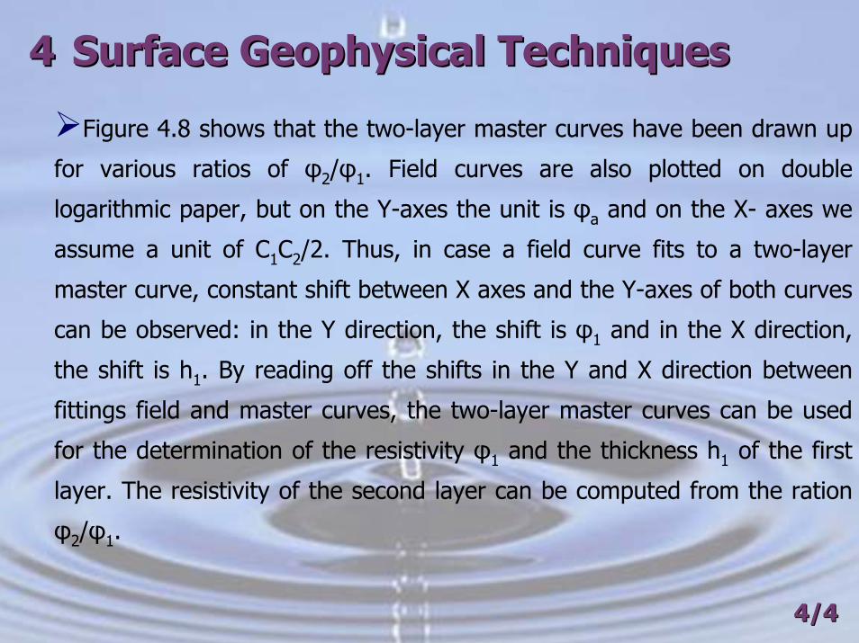
Figure 4.8 shows that the two-layer master curves have been drawn up
for various ratios of φ2/φ1. Field curves are also plotted on double
logarithmic paper, but on the Y-axes the unit is φa and on the X- axes we
assume a unit of C1C2/2. Thus, in case a field curve fits to a two-layer
master curve, constant shift between X axes and the Y-axes of both curves
can be observed: in the Y direction, the shift is φ1 and in the X direction,
the shift is h1. By reading off the shifts in the Y and X direction between
fittings field and master curves, the two-layer master curves can be used
for the determination of the resistivity φ1 and the thickness h1 of the first
layer. The resistivity of the second layer can be computed from the ration
φ2/φ1.
4/44/4

44 Surface Geophysical TechniquesSurface Geophysical Techniques
Figure 4.8: Two layer Master Curves
4/44/4
44 Surface Geophysical TechniquesSurface Geophysical Techniques
Three layers master curves: master curves for the three-layer case
cannot be presented in a single diagram. Sets of three-layer master curves
can be classified according to their shape. Figure 4.9 presents examples
of each of the four types of three-layer master curves. In these curves the
first layer is reflected in the left hand side of the curve; the middle layer is
reflected in a maximum, minimum or a distinctive change in slope in the
ascending and descending segment somewhere in the middle of the curve,
and the third layer corresponds to the right hand side of the curve.
4/44/4

44 Surface Geophysical TechniquesSurface Geophysical Techniques
Figure 4.9: Types of three Layer Master Curves
4/44/4
44 Surface Geophysical TechniquesSurface Geophysical Techniques
4.1.6 Porewater Resistivity
The resistivity of a subsurface layer (formation resistivity) depends on:
Porewater resistivity;
Rock type pore space (porosity);
Water content of the rock.
4/44/4
44 Surface Geophysical TechniquesSurface Geophysical Techniques
The porewater resistivity is determined by the properties of the
groundwater in pores, joints, fractures and solution holes contained in
rock. Properties include the concentration of total solids in solution, the
type of ions dissolved and water temperature. Therefore, the porewater
resistivity is also a measure of the groundwater quality. The influence of
the concentration of total dissolved solids is most influential. The higher
the concentration of total dissolved solids, the higher is the water
conductivity, and the lower is the porewater resistivity. This relationship is
shown in Figure 4.10, where the concentration of two of the most
common solids dissolved in groundwater (sodium chloride NaCl, and
sodium bicarbonate NaHCO3), are set out against the water conductivity
and the water resistivity of the solution.
4/44/4

44 Surface Geophysical TechniquesSurface Geophysical Techniques
Figure 4.10: Relation between concentration and resistivity
4/44/4
44 Surface Geophysical TechniquesSurface Geophysical Techniques
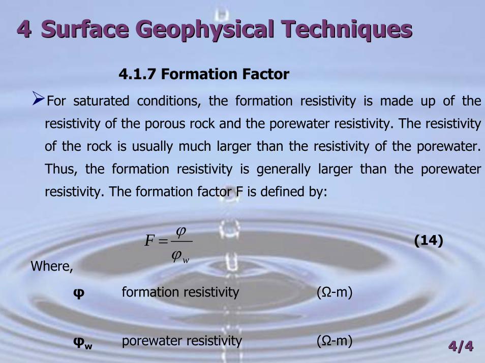
4.1.7 Formation Factor
For saturated conditions, the formation resistivity is made up of the
resistivity of the porous rock and the porewater resistivity. The resistivity
of the rock is usually much larger than the resistivity of the porewater.
Thus, the formation resistivity is generally larger than the porewater
resistivity. The formation factor F is defined by:
(14)
Where,
φ formation resistivity (Ω-m)
φw porewater resistivity (Ω-m) 4/44/4
w
Fϕϕ
=
44 Surface Geophysical TechniquesSurface Geophysical Techniques
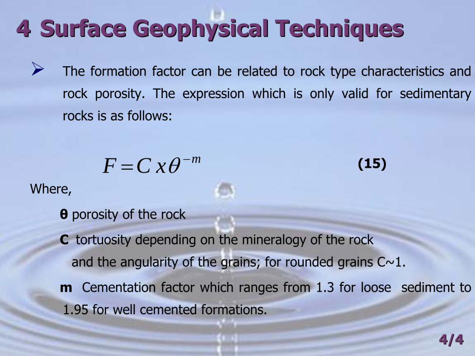
The formation factor can be related to rock type characteristics and
rock porosity. The expression which is only valid for sedimentary
rocks is as follows:
(15)
Where,
θ porosity of the rock
C tortuosity depending on the mineralogy of the rock
and the angularity of the grains; for rounded grains C~1.
m Cementation factor which ranges from 1.3 for loose sediment to
1.95 for well cemented formations.
4/44/4
mxCF −= θ

44 Surface Geophysical TechniquesSurface Geophysical Techniques
The formation factor for unconsolidated sediments ranges from about
1 to 6 ( e.g. for clays F is in the 1-2 range, while for coarser sands, F
values in the order of 5-6 are common). Table 4.2 gives a summary
of formation factors common for unconsolidated sediments. In the
more consolidated sediments the porosities are usually lower and
formation factors for these rocks tend to be higher.
4/44/4

44 Surface Geophysical TechniquesSurface Geophysical Techniques
Table 4.2: formation factors for some unconsolidated sediments
FLithology
7.565
4.23.5
<2.5
GravelCoarse sand and gravel
Coarse sanMedium sand
Fine sandClayey sand
4/44/4
44 Surface Geophysical TechniquesSurface Geophysical Techniques
4.1.8 Hydrogeological Interpretation Procedures
The interpretation means in the first place that we will have to
associate the formation resistivities (rock layer resistivities)
determined at geo-electrical measurement sites with rock types, rock
water contents and porewater resistivities. Follow the resistivity
allocation and correlation procedure:
Allocation is the assignment of rock type and formation factor, rock
water content, and porewater resistivity or conductivity value
interpreted at an individual geo-electrical measurement site. The
formation which is compiled on the so-called calibration tables should
be used to complete these activities. Preferably, calibration tables are
prepared on the basis of data collected during an exploration drilling
programme. 4/44/4

44 Surface Geophysical TechniquesSurface Geophysical Techniques
Correlation is the activity whereby the interpreted formation
resistivities at the various individual measurement sites are compared
with each other. Correlation may first be carried out on the basis of
resistivity values alone and then be finalized after rock characteristics
have been assigned (see above). This can best be carried out by setting
up cross sections along the lines of geo-electrical measurement sites and
any exploration wells on these lines. Subsurface layers with similar
characteristics on these sections may be connected with each other,
presenting an excellent view of the (hydro)geological conditions within
an investigated area.
See Table 4.3 as an example for calibration of porewater resistivity
4/44/4

44 Surface Geophysical TechniquesSurface Geophysical Techniques
Table 4.3: Example of a calibration table (the Rada
Area in Yamen)Porewater φ
(Ω-m)Water
ContentRock TypeFormation φ (Ω-
m)
< 3.3 (brackish)10 – 25 (fresh)10 – 25 (fresh)10 – 25 (fresh)
SaturatedSaturatedSaturatedSaturated
Unsaturated Dense rock
Alluvial sandAlluvial sandWeathered basementSandstone
Alluvial sandBasement gneiss
< 1030 - 70
30 - 10080 - 200> 1000> 1000
4/44/4

4.1.9 Interpretation Hazards
The use of allocation and correlation techniques for geoelectrical
interpretation may be complicated or tricky for a number of reasons. First, the
formation resistivities at the measurement sites may be considerably higher or
lower than the range of values offered by the calibration table.
Secondly, it is normally assumed that in case the formation resistivity values
at the measurements sites and at the exploration, drilling sites are similar, the
φw and F values are also similar. This is not always correct. Formation
resistivities in an investigation area would not show any spatial variation as
long as the product [Fx φw] is constant. The case may present itself that at a
geo electrical measurement site this product is indeed the same as at
exploration drilling sites, but that nevertheless, the F and the φw are quite
different. We are then inclined to make an interpretation error. Only when we
have a good perception of the area interpretation errors like these can be
avoided.
44 Surface Geophysical TechniquesSurface Geophysical Techniques
4/44/4
44 Surface Geophysical TechniquesSurface Geophysical Techniques
4.1.10 Data Interpretation for Constant Electrode
Distance
For the Wenner arrangement (constant electrode distance survey),
the apparent resistivity values for the successive measurement positions
can be calculated from Eq. 11. For reconnaissance, surveying the
apparent resistivities can be plotted on a topographical or geological
map. Contour lines (iso-resistivity lines) may be drawn on these maps
and sub-areas with typical apparent resistivity values can be delineated.
For “discontinuity” surveying a plot may be made showing distances to
the measuring points from the start of the section line (on x axis) against
the corresponding apparent resistivity values (on y axes). 4/44/4

SESSION 10SESSION 10
GROUNDWATER EXPLORATIONGROUNDWATER EXPLORATIONIIIIII
Dr Amjad AliewiDr Amjad Aliewi
House of Water and Environment
Email: [email protected] , Website: www.hwe.org.ps
44 Surface Geophysical TechniquesSurface Geophysical Techniques
The hydrological interpretation based on measurements following the
constant electrode distance technique is a rather qualitative
interpretation. For the case of reconnaissance surveying the rock type,
the rock water content or the porewater resistivity can also be estimated
for a selected investigation depth. Only estimates are possible.
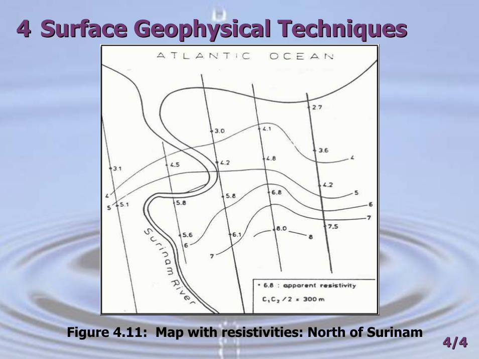
Figure 4.11 shows an apparent resistivity map for the North of
Surinam gives details. The coastal groundwater basin underlying the
area consists of unconsolidated sediments up to several hundreds of
meters of unconsolidated sediments up to several hundreds of meters
below ground surface. The resistivity values and iso-resistivity lines
which are shown on the map correspond with an investigation depth of
150 to 200 m below ground surface. The interpretation is as follows:4/44/4
44 Surface Geophysical TechniquesSurface Geophysical Techniques
The sub-area near to the coastline with relatively low formation
resistivities in the order of 2.5 to 5 Ω-m point to low porewater
resistivities. This correlates with the occurrence of brackish to saline
groundwater at the elected investigation depth.
For similar depths ranges, the higher resistivities in the order of 6 to
8 Ω-m for the sub-areas farther inland represent fresh to brackish
groundwater.
4/44/4
44 Surface Geophysical TechniquesSurface Geophysical Techniques
Figure 4.11: Map with resistivities: North of Surinam4/44/4

44 Surface Geophysical TechniquesSurface Geophysical Techniques
When surveying for “discontinuities” the hydrogeological interpretation
is also largely qualitative. For example, fault zones usually have higher
water contents than the surrounding rock. This is reflected in a low
apparent resistivity. Thus, a fault can be detected by low apparent
resistivity values in a measurement series. Let us consider another
example of a “discontinuity”: a dolerite dike. Dikes may be associated with
a low formation factor due to the presence of conductive iron-containing
minerals. This will also be reflected in low apparent resistivity values which
will be indicated when surveying across the dike. We can conclude from
the above that an interpretation of apparent resistivity data cannot stand
alone: they have to be considered in combination with data from other
sources.4/44/4
44 Surface Geophysical TechniquesSurface Geophysical Techniques
4.1.11 CASE STUDY (Driscoll, pp 179-181)
A consultant was retained by a developer to locate suitable groundwater
supply for a proposed mobile home park.
A test well drilled on the northwest potion of the property to a depth of
250 ft, encountered about 50 to 60 ft of fine sand. The yield was about
100 gpm, much less than the developer required. The consultant
recommended that a surface resistivity survey be conducted over the
entire parcel to define the most promising area for another well.
4/44/4
44 Surface Geophysical TechniquesSurface Geophysical Techniques
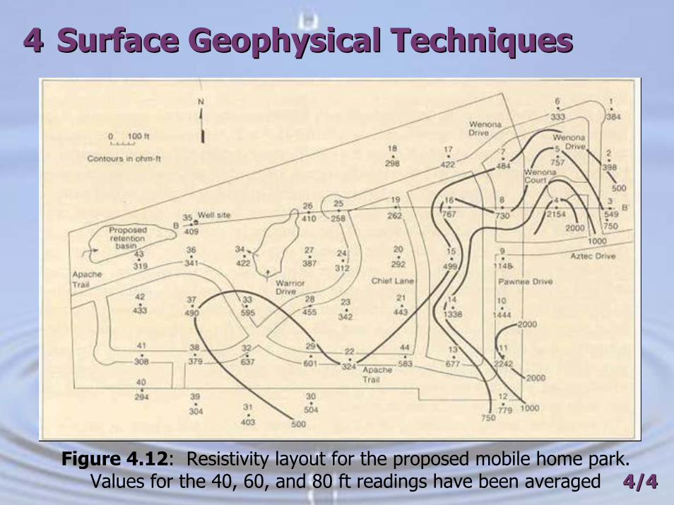
A resistivity survey consisting of 44 stations was laid out on a grid
shown in Figure 4.12. Earth resistivity was taken with a Wenner array
using 10, 20, 40, 60, 80, 120 and 160 ft a-spacing readings. These data
enabled the consultant to construct an apparent resistivity/depth profile at
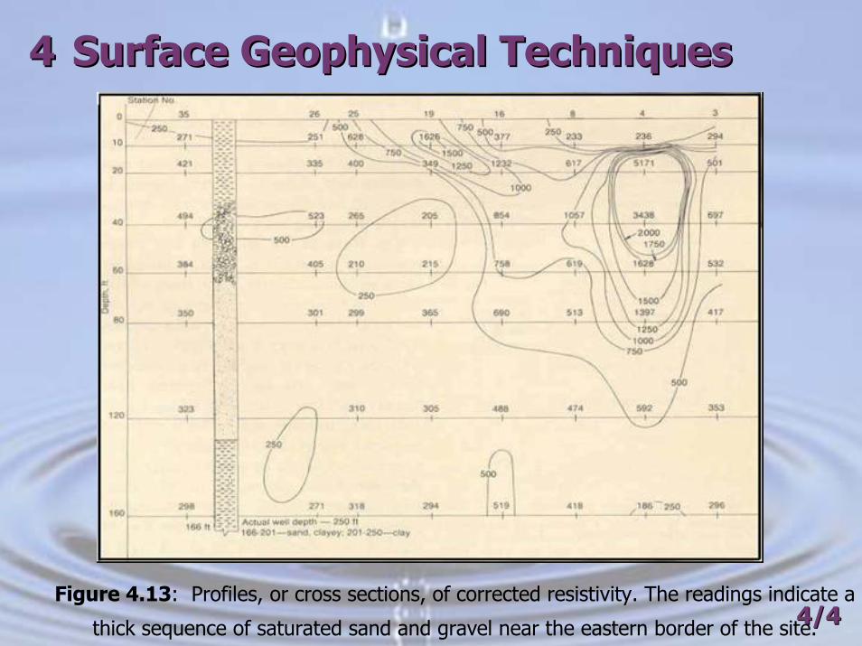
each location. Cross sections of corrected resistivity were plotted in Figure
4.13. The profiles were contoured and then studied to determine whether
any particular depth intervals displayed high values of resistivity which
would indicate the presence of saturated sand and gravel lenses.
4/44/4
44 Surface Geophysical TechniquesSurface Geophysical Techniques
4/44/4Figure 4.12: Resistivity layout for the proposed mobile home park.
Values for the 40, 60, and 80 ft readings have been averaged
44 Surface Geophysical TechniquesSurface Geophysical Techniques
Figure 4.13: Profiles, or cross sections, of corrected resistivity. The readings indicate a
thick sequence of saturated sand and gravel near the eastern border of the site.4/44/4
44 Surface Geophysical TechniquesSurface Geophysical Techniques
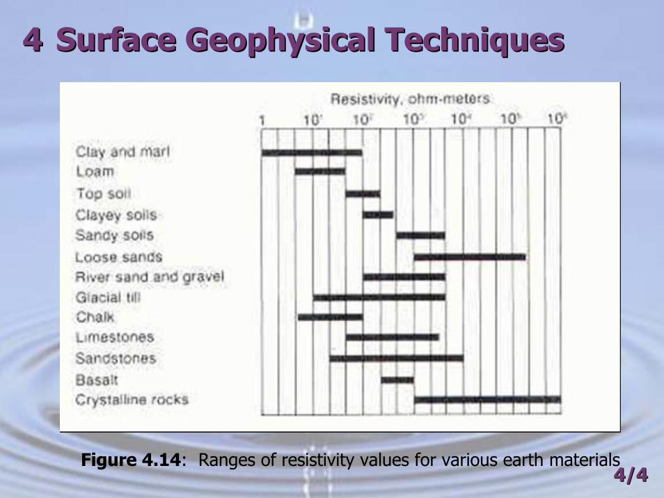
Interpretation of resistivity values obtained from the survey indicate that
aquifer conditions would be much more promising toward the eastern end
of the property. Test drilling was recommended along the line of stations
8, 9, and 10. Ideally, drilling should have occurred along the line of
stations 4, 5 and 6 but this area had already been developed with homes
(see Figure 4.14).
4/44/4
44 Surface Geophysical TechniquesSurface Geophysical Techniques
Figure 4.14: Ranges of resistivity values for various earth materials4/44/4
44 Surface Geophysical TechniquesSurface Geophysical Techniques
Subsequently, a 12-in well was installed to a depth of 90 ft at the
selected location. The boring encountered sand and gravel from a depth of
about 5 ft to the bottom of the boring at 19 ft. during a 24 hour aquifer
test, the well was pumped at 1,250 gpm, the specific capacity was 70 gpm
for 100 days of continuous pumping which far exceeded the short term
100 gpm yield of the original test well a few hundred feet to the West.
4/44/4

44 Surface Geophysical TechniquesSurface Geophysical Techniques
4.2 Surface Electro-Magnetic Techniques
4.2.1 Working Principle
Primary electro-magnetic fields are generated by a transmitter at land
surface. They induce currents at subsurface conductors which include
rock types of a low resistivity. The induced currents produce a
secondary electro-magnetic field that differs in magnitude and
orientation, and in phase from the primary field. A recover measures the
resulting total field. The principle is illustrated in Figure 4.15.
4/44/4

44 Surface Geophysical TechniquesSurface Geophysical Techniques
Figure 4.15: Principles of electro-magnetic techniques
4/44/4
44 Surface Geophysical TechniquesSurface Geophysical Techniques
The receiver measures the phase or the resulting primary plus
secondary field (total field). The phases of the individual primary and
secondary fields can be determined from these measurements. We will find
that the phase of the secondary field generated by the subsurface
conductor differs from the phase of the primary field. The better the
conductor the more lags the phase of the secondary field behind the phase
of the primary magnetic field. For very good conductors the phase of the
secondary field may even lag 180 degrees behind the phase of the primary
field. For poor conductors the phase difference between primary and
secondary magnetic fields is usually in the order of 90 degrees (see Figure
4.16).
4/44/4

44 Surface Geophysical TechniquesSurface Geophysical Techniques
Figure 4.16: primary and secondary magnetic fields
4/44/4
44 Surface Geophysical TechniquesSurface Geophysical Techniques
Field strengths for the secondary field can be computed from the
measurements recorded by the receiver. These field strengths can be used
to find implicit values for the resistivities of subsurface conductive rock
layers.
4/44/4
44 Surface Geophysical TechniquesSurface Geophysical Techniques
4.2.2 Variable Electrode Distance Geo-electrical
Technique
ADVANTAGES
It can be used for the exploration of underground in a large variety of
areas with diverse geological conditions.
It is still the superior surveying techniques when information on the
individual subsurface rock layers is required.
The time needed for surveying and interpretation can be shortened.
4/44/4

44 Surface Geophysical TechniquesSurface Geophysical Techniques
DISADVANTAGES
A large entry resistance at the current electrodes (very dry conditions)
may jeopardize the measurements. Mineralized water is usually added to
improve conditions.
In areas with very low layer resistivities (brackish to saline
groundwater), the potential differences to be measured may be too small
and cannot be accurately measured. Working with larger currents may
help.
The method is still time consuming and expensive. In comparison with
other geophysical techniques survey time may be 3 to 4 times as long.4/44/4
44 Surface Geophysical TechniquesSurface Geophysical Techniques
4.2.3 Electro-Magnetic Techniques
These are often considered compatible with Geo-electrical techniques.
In particular electro-magnetic surveys are thought to be in the same
league as the Geo-electrical surveys following the constant electrode
distance arrangement. Engaged in reconnaissance surveying, both
techniques can be used to obtain a quick impression of the resistivities
of the subsurface layers in an area. Also, both techniques are well suited
for tracking down vertical or steeply dipping “discontinuities” such as
fault zones or intrusive dykes and sills in hard rock areas.
4/44/4

44 Surface Geophysical TechniquesSurface Geophysical Techniques
ADVANTAGES
Electro-magnetic surveying is faster than Geo-electrical surveying
following the constant electrode distance technique.
Electro-magnetic surveying is relatively inexpensive. Capital investment
for some of the instrument is similar to the acquisition cost of Geo-
electrical equipment. The cost gain is in time and in labor. For electro-
magnetic surveying one or two men are usually required, while in Geo-
electrical surveying at least three men will have to be employed (see
Figure 4.17).
4/44/4
44 Surface Geophysical TechniquesSurface Geophysical Techniques
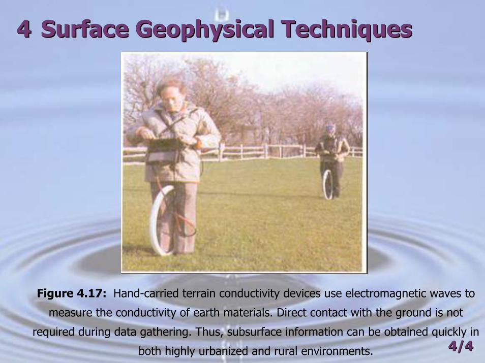
Figure 4.17: Hand-carried terrain conductivity devices use electromagnetic waves to
measure the conductivity of earth materials. Direct contact with the ground is not
required during data gathering. Thus, subsurface information can be obtained quickly in
both highly urbanized and rural environments. 4/44/4
44 Surface Geophysical TechniquesSurface Geophysical Techniques
In case surface layers with a sufficiently high resistively are present then
the electro-magnetic method is ideally suited to unravel conductive rock
layers, or bodies etc at larger depths. This is done for relatively small
transmitter-receiver spacings. If we employ Geo-electrical techniques
following the constant electrode distance method large electrode spacings
are needed and more geological details may be lost. Such detail could have
been detected if an electro-magnetic survey would have been set up.
Electro-magnetic surveying may work better in case we deal with
resistive surface layers. The magnetic fields that we use in electro-
magnetic surveying are by no means hampered by such layers. On the
other hand, electric currents which we use in Geo-electrical surveying may
be obstructed due to large entry resistance.
4/44/4
44 Surface Geophysical TechniquesSurface Geophysical Techniques
DISADVANTAGES
Electro-magnetic surveying is severely hindered by the presence of
man-made conductors, e.g. power lines, buried pipes, cables and wire
fences.
In case surface layers have a low resistivity then the electro-magnetic
response tends to be primarily generated by these layers. There will be an
inadequate response of any deeper rock layers, or these layers may not
even be detected.
Interpretation may be carried out in a qualitative way. There is no direct
information on rock properties such as apparent rock resistivities. 4/44/4
44 Surface Geophysical TechniquesSurface Geophysical Techniques
4.3 Seismic Refraction Method
4.3.1 Working Principle
The seismic refraction method is based on the fact that elastic waves
travel through different earth materials at different earth velocities. The
denser the material, the higher the wave velocity.
The waves are called elastic because as the waves pass a point in the
rock, the particles are momentarily displaced or distorted but
immediately return to their original position or shape after wave passes;
4/44/4
44 Surface Geophysical TechniquesSurface Geophysical TechniquesThree types of waves can be created: Compressional waves (P), Shear
waves (V), and surface waves. Compressional waves are the first to arrive
at the geophones and therefore are the most useful in seismic surveys;
In general, the higher the density and elasticity of the rock unit, the
faster the P wave will be transmitted. The velocity is much less and the
energy is dissipated more quickly if the material is unconsolidated or poorly
consolidated.
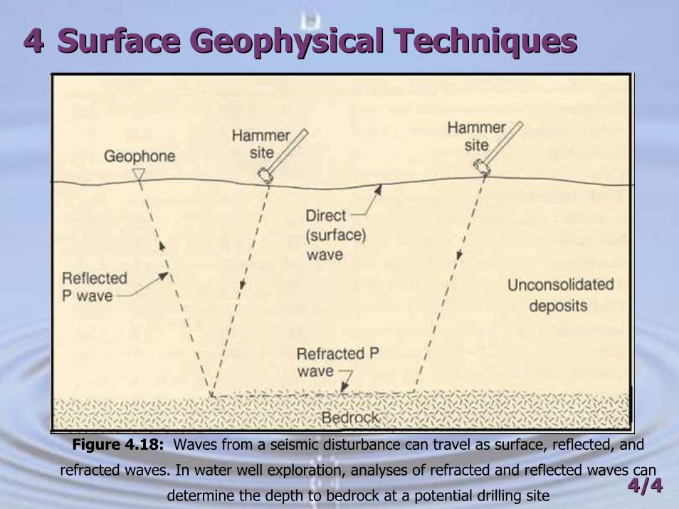
Three distinct paths are taken by compressional waves in the ground:
direct, refracted and reflected (see Figure 4.18). A single seismic impulse
can be recorded as three separate arrivals at the geophone. In practice,
however, only the first arrival can be readily recognized. 4/44/4
44 Surface Geophysical TechniquesSurface Geophysical Techniques
Figure 4.18: Waves from a seismic disturbance can travel as surface, reflected, and
refracted waves. In water well exploration, analyses of refracted and reflected waves can
determine the depth to bedrock at a potential drilling site 4/44/4
44 Surface Geophysical TechniquesSurface Geophysical Techniques
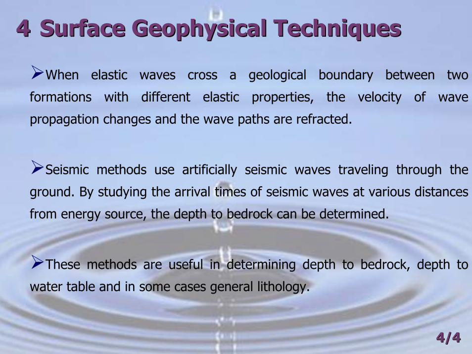
When elastic waves cross a geological boundary between two
formations with different elastic properties, the velocity of wave
propagation changes and the wave paths are refracted.
Seismic methods use artificially seismic waves traveling through the
ground. By studying the arrival times of seismic waves at various distances
from energy source, the depth to bedrock can be determined.
These methods are useful in determining depth to bedrock, depth to
water table and in some cases general lithology.
4/44/4
44 Surface Geophysical TechniquesSurface Geophysical Techniques
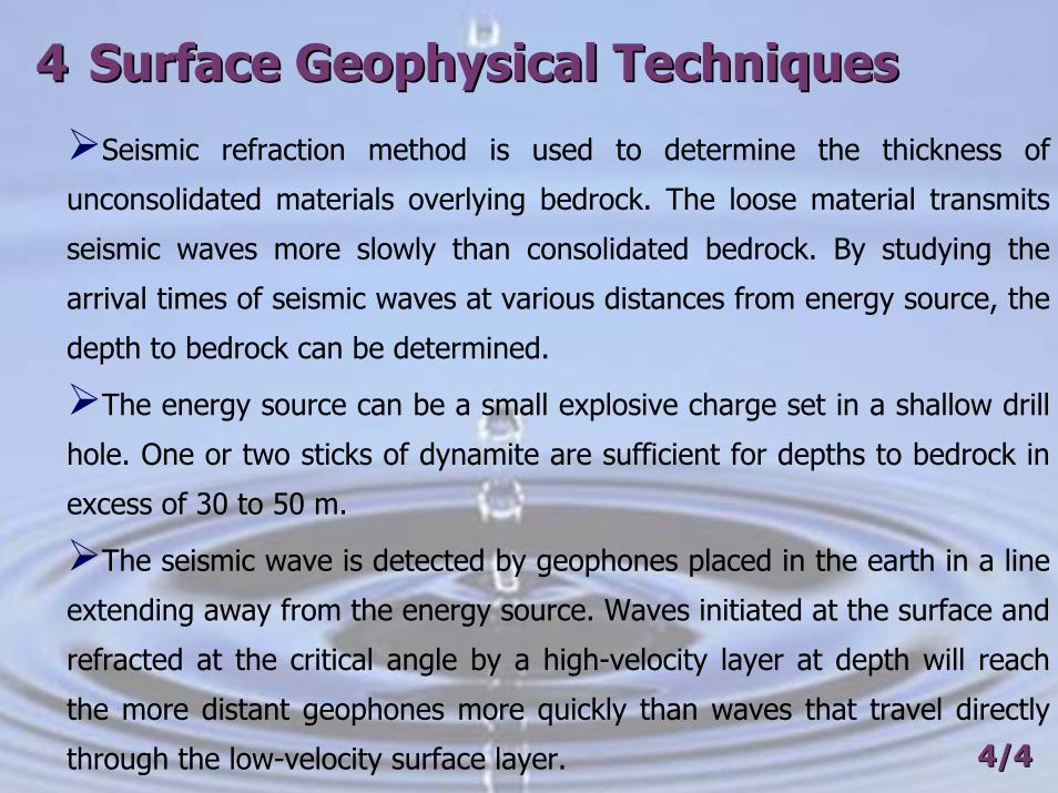
Seismic refraction method is used to determine the thickness of
unconsolidated materials overlying bedrock. The loose material transmits
seismic waves more slowly than consolidated bedrock. By studying the
arrival times of seismic waves at various distances from energy source, the
depth to bedrock can be determined.
The energy source can be a small explosive charge set in a shallow drill
hole. One or two sticks of dynamite are sufficient for depths to bedrock in
excess of 30 to 50 m.
The seismic wave is detected by geophones placed in the earth in a line
extending away from the energy source. Waves initiated at the surface and
refracted at the critical angle by a high-velocity layer at depth will reach
the more distant geophones more quickly than waves that travel directly
through the low-velocity surface layer. 4/44/4
44 Surface Geophysical TechniquesSurface Geophysical Techniques
4.3.2 Interpretation
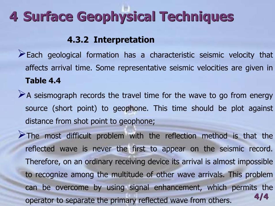
Each geological formation has a characteristic seismic velocity that
affects arrival time. Some representative seismic velocities are given in
Table 4.4
A seismograph records the travel time for the wave to go from energy
source (short point) to geophone. This time should be plot against
distance from shot point to geophone;
The most difficult problem with the reflection method is that the
reflected wave is never the first to appear on the seismic record.
Therefore, on an ordinary receiving device its arrival is almost impossible
to recognize among the multitude of other wave arrivals. This problem
can be overcome by using signal enhancement, which permits the
operator to separate the primary reflected wave from others. 4/44/4
44 Surface Geophysical TechniquesSurface Geophysical Techniques
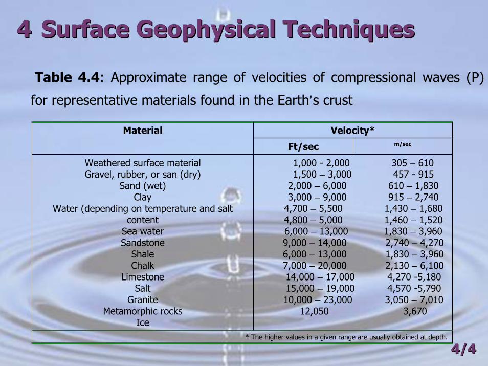
Table 4.4: Approximate range of velocities of compressional waves (P)
for representative materials found in the Earth’s crust
4/44/4
Velocity*m/secFt/sec
1,000 - 2,000 305 – 6101,500 – 3,000 457 - 915
2,000 – 6,000 610 – 1,8303,000 – 9,000 915 – 2,740
4,700 – 5,500 1,430 – 1,6804,800 – 5,000 1,460 – 1,520 6,000 – 13,000 1,830 – 3,9609,000 – 14,000 2,740 – 4,2706,000 – 13,000 1,830 – 3,9607,000 – 20,000 2,130 – 6,10014,000 – 17,000 4,270 -5,18015,000 – 19,000 4,570 -5,79010,000 – 23,000 3,050 – 7,010
12,050 3,670
Weathered surface materialGravel, rubber, or san (dry)
Sand (wet)Clay
Water (depending on temperature and salt content
Sea waterSandstone
ShaleChalk
LimestoneSalt
GraniteMetamorphic rocks
Ice* The higher values in a given range are usually obtained at depth.
Material

44 Surface Geophysical TechniquesSurface Geophysical Techniques
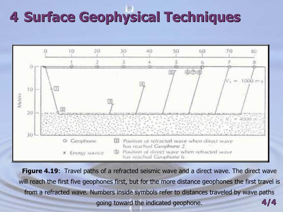
Figure 4.19 illustrates the travel paths of compressive seismic waves
traveling through a two-layer earth. The seismic velocity in the lower layer
is greater than that in the upper layer. As the energy travels faster in the
lower layer, the way passing through it gets ahead of the wave in the
upper layer. At the boundary between the two layers, part of the energy is
refracted back upward from the lower-layer boundary to the surface;
4/44/4
44 Surface Geophysical TechniquesSurface Geophysical Techniques
Figure 4.19: Travel paths of a refracted seismic wave and a direct wave. The direct wave
will reach the first five geophones first, but for the more distance geophones the first travel is
from a refracted wave. Numbers inside symbols refer to distances traveled by wave paths
going toward the indicated geophone. 4/44/4
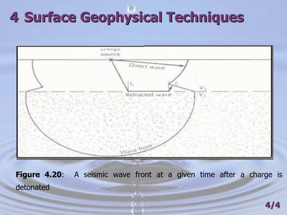
44 Surface Geophysical TechniquesSurface Geophysical TechniquesThe angle of refraction of each wave front is called the critical angle ic,
and is equal to the arc sin of the ration of the velocities of the two layers:
(16)
Figure 4.20 illustrates a wave front and the path of the refracted
energy that travels along the lower-layer boundary. A direct wave in the
upper layer is also shown.
If V2<V1 then the wave will be refracted downward and no energy will
be directed upward. Thus the refraction method will show higher-velocity
layers but no lower-velocity layers that are overlain by a high-velocity
layer. 4/44/4
2
11sinVV
ic−=
44 Surface Geophysical TechniquesSurface Geophysical Techniques
Figure 4.20: A seismic wave front at a given time after a charge is
detonated
4/44/4
44 Surface Geophysical TechniquesSurface Geophysical Techniques
Energy travels directly through the upper layer from the source to the
geophone. This is the shortest distance, but the waves do not travel as fast
as those traveling along the top of the lower layer. The latter go farther,
but with a higher velocity. Figure 4.19 shows the positions of waves
traveling to each geophone. Geophones 1 through 5 first receive waves
that have traveled through only the upper layer. The sixth and succeeding
geophones measure arrival times of refracted waves that have gone
through the high-velocity layer as well. The figure shows the position of
the trailing wave front at each time the leading front reaches each
geophone;
4/44/4
44 Surface Geophysical TechniquesSurface Geophysical Techniques
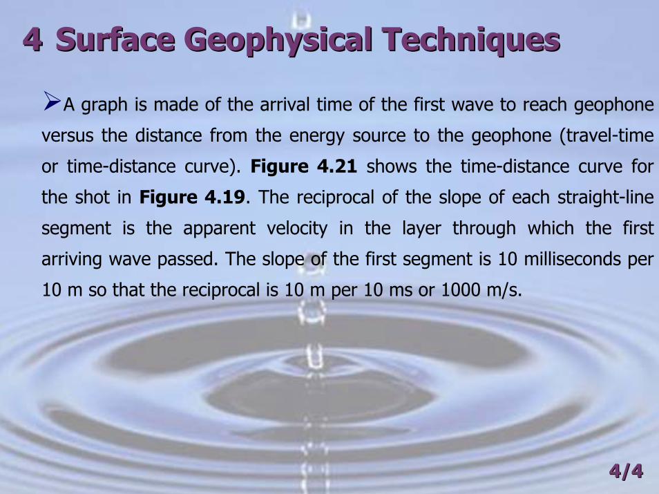
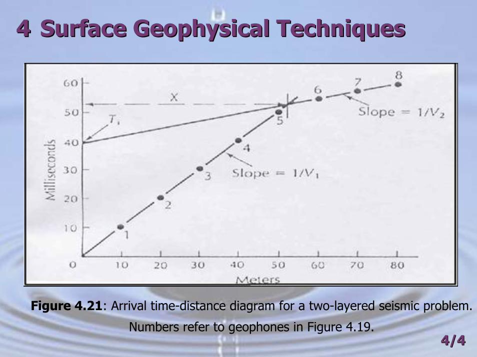
A graph is made of the arrival time of the first wave to reach geophone
versus the distance from the energy source to the geophone (travel-time
or time-distance curve). Figure 4.21 shows the time-distance curve for
the shot in Figure 4.19. The reciprocal of the slope of each straight-line
segment is the apparent velocity in the layer through which the first
arriving wave passed. The slope of the first segment is 10 milliseconds per
10 m so that the reciprocal is 10 m per 10 ms or 1000 m/s.
4/44/4
44 Surface Geophysical TechniquesSurface Geophysical Techniques
Figure 4.21: Arrival time-distance diagram for a two-layered seismic problem.
Numbers refer to geophones in Figure 4.19.4/44/4
44 Surface Geophysical TechniquesSurface Geophysical Techniques
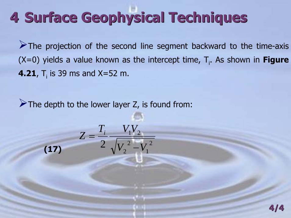
The projection of the second line segment backward to the time-axis
(X=0) yields a value known as the intercept time, Ti. As shown in Figure
4.21, Ti is 39 ms and X=52 m.
The depth to the lower layer Z, is found from:
(17)
4/44/4
21
22
21
2 VV
VVTZ i
−=
44 Surface Geophysical TechniquesSurface Geophysical Techniques
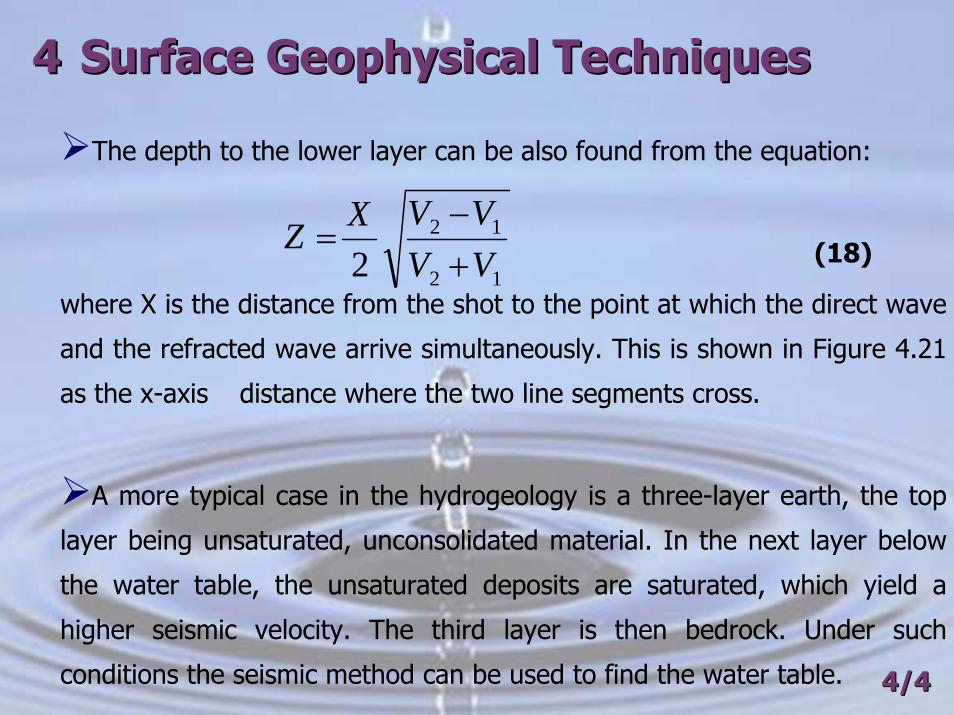
The depth to the lower layer can be also found from the equation:
(18)
where X is the distance from the shot to the point at which the direct wave
and the refracted wave arrive simultaneously. This is shown in Figure 4.21
as the x-axis distance where the two line segments cross.
A more typical case in the hydrogeology is a three-layer earth, the top
layer being unsaturated, unconsolidated material. In the next layer below
the water table, the unsaturated deposits are saturated, which yield a
higher seismic velocity. The third layer is then bedrock. Under such
conditions the seismic method can be used to find the water table. 4/44/4
12
12
2 VVVVXZ
+−
=
44 Surface Geophysical TechniquesSurface Geophysical Techniques
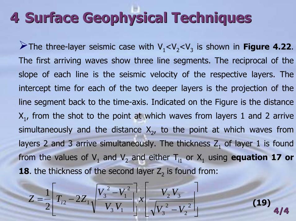
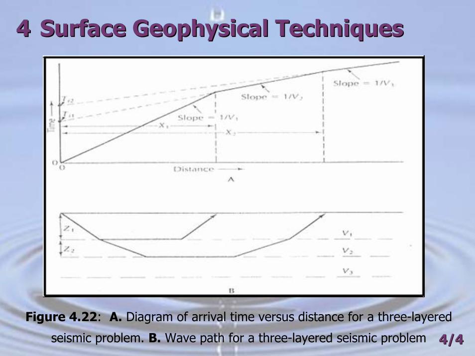
The three-layer seismic case with V1<V2<V3 is shown in Figure 4.22.
The first arriving waves show three line segments. The reciprocal of the
slope of each line is the seismic velocity of the respective layers. The
intercept time for each of the two deeper layers is the projection of the
line segment back to the time-axis. Indicated on the Figure is the distance
X1, from the shot to the point at which waves from layers 1 and 2 arrive
simultaneously and the distance X2, to the point at which waves from
layers 2 and 3 arrive simultaneously. The thickness Z1 of layer 1 is found
from the values of V1 and V2 and either Ti1 or X1 using equation 17 or
18. the thickness of the second layer Z2 is found from:
(19)4/44/4⎥
⎥
⎦
⎤
⎢⎢
⎣
⎡
−⎥⎥⎦
⎤
⎢⎢⎣
⎡ −−=
22
23
32
13
21
23
12 221
VV
VVx
VVVV
ZTZ i
44 Surface Geophysical TechniquesSurface Geophysical Techniques
Figure 4.22: A. Diagram of arrival time versus distance for a three-layered
seismic problem. B. Wave path for a three-layered seismic problem 4/44/4

44 Surface Geophysical TechniquesSurface Geophysical TechniquesThe velocities computed from the reciprocals of the slope are called
apparent velocities. If the lower layer is horizontal, they represent the
actual velocity.
If the lower layer is sloping, the arrival time for a shot measured down
slope will be different from one measured upslope. Seismic lines are
routinely run with a shot at either end, so that dipping beds can be
determined.
Time-distance curves for a dipping stratum are shown in Figure 4.23,
with travel times measured from shots at either end of the line. The upper
layer is unaffected by the dip of the lower bed, so that the reciprocal of the
slope of the first line segment is V1. in order to find the values of V2 and
the depth to the bedrock at the undip end of the line Zd, as well as at the
downdip end Zu, a complex series of computations must be made. 4/44/4
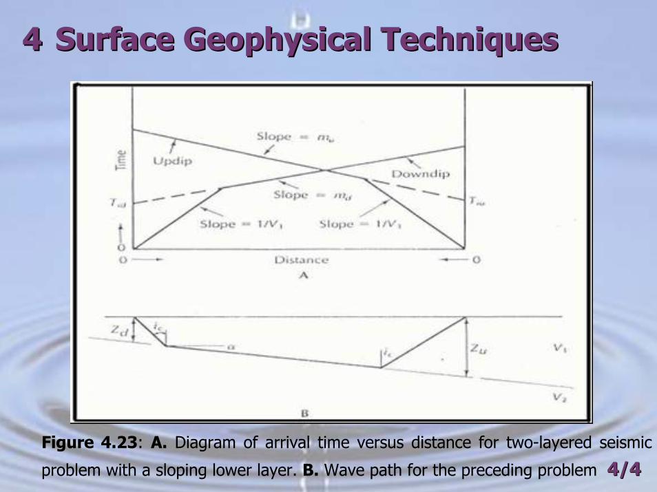
44 Surface Geophysical TechniquesSurface Geophysical Techniques
Figure 4.23: A. Diagram of arrival time versus distance for two-layered seismic
problem with a sloping lower layer. B. Wave path for the preceding problem 4/44/4
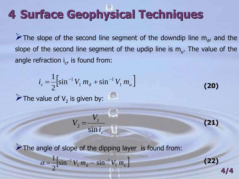
44 Surface Geophysical TechniquesSurface Geophysical Techniques
The slope of the second line segment of the downdip line md, and the
slope of the second line segment of the updip line is mu. The value of the
angle refraction ic, is found from:
(20)
The value of V2 is given by:
(21)
The angle of slope of the dipping layer is found from:
(22)4/44/4
[ ]udc mVmVi 11
11 sinsin
21 −− +=
ciVV
sin1
2 =
[ ]ud mVmV 11
11 sinsin
21 −− −=α

44 Surface Geophysical TechniquesSurface Geophysical Techniques
The depths to the lower layer at either end of the shot line are found
from:
(23)
(24)
4/44/4
)cos2()(cos1
c
iuu i
TVZ
α=
)cos2()(cos1
c
idd i
TVZ
α=