settling disputes at the world trade organization

Settling disputes at the World Trade Organization

Örebro Studies in Economics 38

LOUISE JOHANNESSON

Settling disputes at the World Trade Organization

© Louise Johannesson, 2018

Title: Settling disputes at the World Trade Organization

Publisher: Örebro University 2018 www.oru.se/publikationer-avhandlingar

Print: Örebro University, Repro 02/2018

ISSN 1651-8896 ISBN 978-91-7529-233-5

Abstract Louise Johannesson (2018): Settling disputes at the World Trade Organiza-tion. Örebro Studies in Economics 38 This cumulative dissertation consists of five self-contained essays, all of which are closely focused around issues that concern the WTO dispute settlement mechanism (DSM). In Essay 1, we describe salient features of the DSM using a unique data set. We observe a spike in new disputes in 2012, which in turn led to an increasing number of panels and appeals. This put the WTO under a heavy workload and delays soon became an issue. In Essay 2, we show that the DSM often appoint institutional in-siders to serve as judges. Although the DSM was reformed under the WTO, the judges are similar to those found in the GATT. Furthermore, there is an incentive structure in place that encourage the WTO Secretar-iat to assume a larger role in writing panel reports and for panelists to let them. Essay 3 examines the role of Special and Differential Treatment (SDT) provision Art. 8.10 of the Dispute Settlement Understanding (DSU) in helping developing countries win disputes against richer coun-tries. We observe that developing countries lose more claims when this provision is applied. I formulate a model and show that this observation can be consistent with the presumed benefit of Art. 8.10. Essay 4 ad-dresses the problem of delays by asking ourselves whether we can lessen the problem with a permanent panel. I study features such as the panel-ists’ experience and prior working relationships in explaining the time it takes to issue panel reports and efficiency in examining claims. We find that prior collaboration can decrease duration. Lastly, in Essay 5, we assess the impact on trade for members that are not involved in disputes. There is evidence of positive trade effects after a dispute for non-complainants, but the effects are limited to disputes that did not escalate to adjudication. We found no external dispute effects for adjudicated disputes.

Keywords: World Trade Organization, trade policy, trade disputes, dispute settlement, causality, panels, developing countries, panels, international trade Louise Johannesson, Örebro University School of Business, SE-701 82 Örebro, Sweden, e-mail: [email protected]

mailto:[email protected]

Acknowledgements

“…nothing clears up a case so much as stating it to another person.”

Sherlock Holmes, Silver Blaze

There is nothing truer in research than the above observation. Forming a sentence is a solitary task, but forming a research question takes a village. And my village is populated with the most wonderful people.

It is still baffling to me that I had the extreme fortune to meet a mentor like Professor Henrik Horn. Not only is he a distinguished scholar but also an extraordinary man that helped me to carve out this path in life. It took a long time to get here, longer than for most I believe, but I arrived, in large part due to Henrik’s unwavering support. Research Institute of Industrial Economics (IFN), and especially Professor Magnus Henrekson and Profes-sor Lars Persson, have given me such colossal support over the years. I have been given so many valuable opportunities and it has been a privilege to work at IFN. I am truly grateful for my hard-working supervisors, docent Magnus Lode-falk, Professor Hildegunn Kyvik Nordås and Professor Dan Johansson, who always offered such insightful and helpful comments and suggestions. With-out your perseverance throughout the process, this dissertation would have been impossible to complete. During this time, I was lucky enough to write papers with three fantastic scholars. Professor Petros C. Mavroidis who can only be described as one of a kind. A caring and creative person that seems to always be full of ideas, and possessing the energy to pursue them all. Dr. Shon Ferguson, thank you for all your patience during this time. Your pragmatism and levelheadedness made working with you such a pleasant and fun experience. Although a short collaboration, working with the bright Dr. Emily Lydgate was im-mensely educational. Professor Lars Hultkrantz, the heart of the economics department at Örebro University. I always enjoyed our conversations. Professor Bernard Hoekman at the European University Institute, thank you for inviting me to

Italy and supporting the update of the WTO dispute settlement data set as it was an essential part of this dissertation.

I would also like to express my gratitude to Professor Johan Stennek at Gö-teborg University and docent Maria Persson at Lund University for taking the time to review my papers and offer astute comments and suggestions. The fun and interesting people that I met through DISSETTLE at the Grad-uate Institute of International and Development Studies (IHEID) in Geneva. Jelena, Aksel, Wouter, Tijl, Nicolo, Marios, Laura, Geraldo, Matteo, Eyal and many more. A special thanks goes out to Dr. Theresa Carpenter and Professor Joost Pauwelyn.

I did not have extensive contact with other PhD students during my doctoral studies with the exception of Dr. Aron Berg. It was so much fun sharing office with you, and I miss our crazy long conversations. To my amazing and beautiful friends, Dina Lindgren and Linn Wikstål. I readily acknowledge that it is not easy to be my friend, and even more so when I am doing a Ph.D. But I promise I will never do it again and I am incredibly grateful to have your support through this demanding process.

Dr. Niklas Kaunitz. You are the best. With all my love.

Tack för allt ditt stöd och tålamod pappa.

Stockholm, February 2018 Louise Johannesson

List of Essays

ESSAY I Johannesson, Louise and Mavroidis, Petros C. ‘The WTO Dispute Settlement System 1995-2016: A Data Set and Its Descriptive Statistics’. (2017) Journal of World Trade 51(3): 357–408.

ESSAY II Johannesson, Louise and Mavroidis, Petros C. ‘Black Cat, White Cat: The Identity of the WTO Judges’. (2015) Journal of World Trade 49(4): 685–698.

ESSAY III Johannesson, Louise. ‘The Effect of Panel Composition on Developing Countries’ Success Rate in the WTO Dispute Settlement’ (2016) IFN Working Paper No. 1120.

ESSAY IV Johannesson, Louise. ‘Efficiency gains and time-savings of permanent panels in the WTO dispute settlement’. Manuscript.

ESSAY V Johannesson, Louise. ‘Are WTO disputes public goods?—Dispute effects on the membership’. Manuscript.

List of abbreviations ACWL Advisory Centre on WTO Law

SPS Agreement on Sanitary and Phytosanitary Measures

TBT Agreement on Technical Barriers to Trade

TRIPS Agreement on Trade-Related Aspects of Intellectual Property Rights

AD Anti-Dumping

AB Appellate Body

Art. Article Textiles and Clothing

ATP

ATT Average Treatment of the Treated

BIC Brazil, India, China

BRIC Brazil, Russia, India, China

BRICS Brazil, Russia, India, China, South Africa

Comtrade Commodity Trade Statistics Database

CTG Council for Trade in Goods

CTS Council for Trade in Services

CV Customs Valuation

DEV Developing countries

DD Difference-in-Differences

DG Director-General

DSB Dispute Settlement Body

DSM Dispute Settlement Mechanism

DSU Dispute Settlement Understanding

G2 EU and US

EC European Communities

EU European Union

FOC First Order Condition

GATT General Agreement on Tariffs and Trade

GATS General Agreement on Trade in Services

GP Government Procurement

HS Harmonized System

IL Import-Licensing Procedures

IND Industrialized countries

ICJ International Court of Justice

ITO International Trade Organization

LDC Least Developed Countries

MFN Most Favoured Nation

MAS Mutually Agreed Solutions

NT National Treatment

OECD Organization of Economic Cooperation and Development

PI Pre-shipment Inspection

RPT Reasonable Period of Time

ROO Rules of Origin

SOC Second Order Condition

SDT Special and Differential Treatment

SCM Subsidies and Countervailing Measures

SG The Agreement on Safeguards

TRIMs Trade-Related Investment Measures

TTIP Transatlantic Trade and Investment Partnership

TPP Trans‐Pacific Partnership

UN United Nations

US United States

WP Working Procedures

WTO World Trade Organization

Table of Contents

1. INTRODUCTION .......................................................................... .... 13

2. AN ESSAY ON THE DISPUTE SETTLEMENT MECHANISM .... .... 18

The WTO Dispute Settlement System 1995-2016: A Data Set and Its Descriptive Statistics (Essay 1) ........................................................ ... 18

3. ESSAYS REGARDING THE FUNCTIONING OF THE PANEL ... ... 21

Black Cat, White Cat: The Identity of the WTO Judges (Essay 2) ..... 21

The Effect of Panel Composition on Developing Countries’ SuccessRate in the WTO Dispute Settlement (Essay 3) .............................. ... 22

Efficiency gains and time-savings of permanent panels in the WTO dispute settlement (Essay 4) ............................................................ ... 24

4. AN ESSAY ON TRADE AND DISPUTES ...................................... .... 26

Are WTO disputes public goods?—Dispute effects on the membership (Essay 5) ......................................................................................... ... 26

5 LIMITATIONS AND METHODOLOGICAL CONSIDERATIONS ....... 28

6. A LOOK FORWARD ..................................................................... .... 31

REFERENCES .................................................................................... ... 33

APPENDIX: ESSAYS 1–5

LOUISE JOHANNESSON Settling disputes at WTO - 13 -

1. Introduction Before the establishment of the World Trade Organization (WTO), and right after the Second World War in 1945, many nations experienced the aftermath of war and felt an urgency to rebuild a shattered world into a better world, based on collaboration and security. In this new world order trade was seen as a cornerstone and an instrument to raise employment and create wealth for all. However, the destructive unilateral trade policies of the interwar period, after the passing of the Smoot-Hawley Act (1930), con-vinced most nations that the expansion of trade was possible only through collective actions and binding commitments. Ambitions were high and to ensure that such an undertaking would be successful, the creation of an In-ternational Trade Organization (ITO) that could provide the necessary or-ganizational structure was proposed (United States. Department of State and Clayton, 1945). Over 50 countries worked together to establish the rules of global trade and bring ITO into existence, but in the end, the agree-ment failed to be ratified by the US after the Truman administration realized that it lacked both public and congressional support.

In the wake of this failed agreement, a smaller group of countries: Aus-tralia, Belgium, Brazil, Burma, Canada, Ceylon, Chile, China, Cuba, Czech-oslovakia, France, India, Lebanon, Luxembourg, Netherlands, New Zea-land, Norway, Pakistan, Southern Rhodesia, Syria, South Africa, the United Kingdom and the US, referred to collectively as the founding members, sal-vaged the commercial policy chapter of the ITO and implemented a provi-sional trade agreement called the General Agreement on Tariffs and Trade (GATT). Across eight trade negotiating rounds, the GATT expanded both its membership and commitments; in each round, several thousands in tariff concessions, worth several billions in trade, were exchanged. In the last round, the Uruguay round, large structural reforms were on the agenda, resulting in the establishment of a new ITO, named the World Trade Or-ganization (WTO). At the time of this organisation’s inauguration, 128 countries had signed the GATT. Since then, 36 more countries, including major countries such as China and Russia, have joined the WTO. At the time of this writing, the WTO has been in operation for over 20 years and over 95% of world trade is now covered by this multilateral trade agree-ment. One of the major innovations in the WTO was its dispute settlement mechanism (DSM), which approached trade disputes between members in a formal and judicial manner. Although a DSM was also available in the

- 14 - LOUISE JOHANNESSON Settling disputes at WTO

GATT, it was less formalized and dispute resolution gravitated towards di-plomacy. The GATT DSM was, nevertheless, quite successful and utilized relatively often, but it had a crucial weakness that undermined the stability of the system.

The first complaint in the GATT came as early as 1948 and at that time, there were no established procedures for resolving complaints, other than requesting bilateral consultations under Art. XXII and Art. XXIII: 1 of the GATT. By the third complaint, however, the disputes were more formally assigned to working party groups—consisting of the parties to the dispute, a chairman and other interested parties—that were composed explicitly for the purpose of resolving the dispute. In 1952, a dispute was, for the first time, referred to a panel of experts for an independent assessment. This task also required the panel to write a formal report of their findings, similar to the current WTO DSM panel reports. Over the next 40 years, 181 panels were established and over 140 panel reports were issued (Busch and Rein-hardt, 2003). However, because the GATT was a provisional agreement, it lacked proper organizational structure. Hence, decisions were made through positive consensus; one such decision was to establish a panel and to adopt the rulings contained in panel reports. Positive consensus implied that, any GATT member could block the adjudication process by rejecting the establishment of a panel, including the parties to the dispute. This rather serious flaw created much uncertainty in the system and was thus removed from the WTO in favour of negative consensus. In other words, panels were established and reports were adopted automatically unless all members agreed otherwise. This was the single most important change from the GATT DSM to the WTO DSM. Other structural changes included the es-tablishment of explicit deadlines at every stage, more detailed procedures surrounding the DSM, and not least, a second instance court, the Appellate Body. So far, 537 complaints have been filed, or 24 complaints per year, compared to the 355 complaints in the GATT (1948–1994), or almost 8 complaints per year (Busch and Reinhardt, 2003). This outcome have led many to hail the DSM as the crowning achievement of the WTO.

However, despite the resounding success of the WTO DSM, some of the concerns that arose in the GATT DSM, as described in Tuthill et al. (1985) ten years before the establishment of the WTO, largely reflect today's prob-lems: delays in panel composition; long panel deliberations; the difficulty in finding qualified and sufficiently independent panelists in regards to nation-ality, experience and governmental interests, and issues for developing countries, such as equal access to the DSM, the lack of retaliatory power,


and fear of retaliation by larger nations. As the GATT DSM became more judicial through the establishment of panels, further issues emerged, such as the need for legal expertise and staff and the high cost of litigation. Why is this the case?

First, the legalization of the DSM sought to ensure equal access to dispute resolution, especially for poorer nations, by creating a system that relies on rules rather than power. However, while access is equal, it is still costly to successfully pursue disputes. At the end of the GATT, only approximately 30% of the contracting parties had been active in the GATT DSM and over 90% of the cases involved either the EU or the US (Tuthill et al., 1985; Hudec et al., 1993). Today, the share of active members has increased only slightly to 35%, while the EU and the US are involved in little over 70% of the cases. With the exception of South Africa, none of the African countries have initiated a dispute. Hence, while the frequency of use has increased substantially, the selection of participants remains relatively narrow, indi-cating that the cost of litigation continues to be an issue.

Figure 1: Time from panel circulation to the adoption of the report

Second, due to the principle of positive consensus in the GATT, signifi-cant delays in both the composition of the panel and adoption of the panel


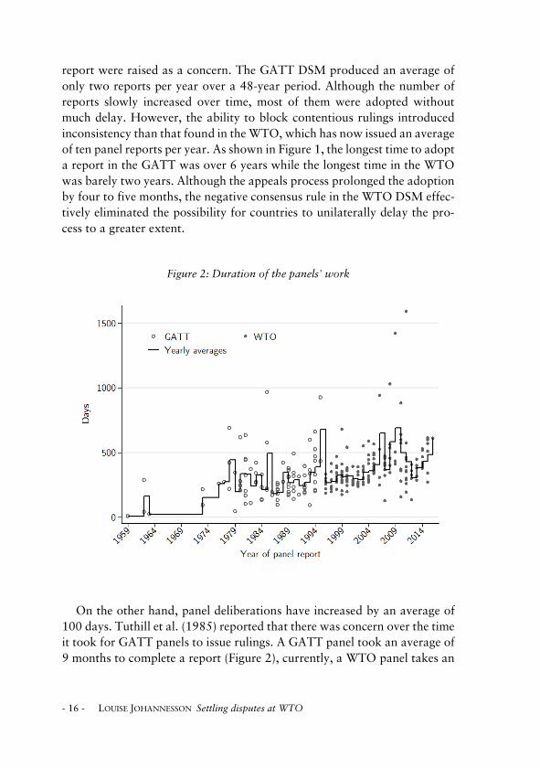
report were raised as a concern. The GATT DSM produced an average of only two reports per year over a 48-year period. Although the number of reports slowly increased over time, most of them were adopted without much delay. However, the ability to block contentious rulings introduced inconsistency than that found in the WTO, which has now issued an average of ten panel reports per year. As shown in Figure 1, the longest time to adopt a report in the GATT was over 6 years while the longest time in the WTO was barely two years. Although the appeals process prolonged the adoption by four to five months, the negative consensus rule in the WTO DSM effec-tively eliminated the possibility for countries to unilaterally delay the pro-cess to a greater extent.

Figure 2: Duration of the panels' work

On the other hand, panel deliberations have increased by an average of

100 days. Tuthill et al. (1985) reported that there was concern over the time it took for GATT panels to issue rulings. A GATT panel took an average of 9 months to complete a report (Figure 2), currently, a WTO panel takes an


average of 12 months—although this does not reflect improvements in effi-ciency as the level of complexity has increased. This is perhaps not surpris-ing because the panel process in the WTO is the same as that in the GATT; namely, a new panel of judges is selected for each dispute. Although proce-dural improvements have been made around the WTO panel stage, such as explicit time-frames, operational rules and notifications, it is still difficult to find eligible and qualified judges who are prepared to spend the time and effort needed on, basically, a part-time assignment.

Figure 3: Panel reports issued

Lastly, the exceptionally long appeal in 2012, shown in Figure 2, was the

beginning of a period of persistent delays caused by an increasing use of the DSM combined with limited staff capacity at the WTO. Although the fre-quent use of the WTO DSM has been seen as a positive development, as shown in Figure 3, this was a trend that, to some extent, began around


1978.1 Hence, even though the structural reforms in the WTO enabled more members to complain, it is likely that the WTO DSM was introduced at a time when the members were strongly committed to resolving trade conflicts in a constructive manner. However, today, this commitment is seemingly starting to wane because the above systemic problems risk undermining the system.

We begin this dissertation by introducing the reader to the WTO DSM and describing some of its salient features (Essay 1). Three of the essays concern the functioning of the panel such as the panel composition process and the identity of the appointed judges in both panels and the Appellate Body. We especially note the considerable role of the WTO Secretariat in supporting these judges (Essay 2). As the issue of delays is becoming more significant, we investigate whether there are any time-saving gains of replac-ing the ad hoc panels described above, with permanent panels (Essay 4). The problem of engaging developing countries in the DSM is studied by evaluating preferential treatment in panel composition (Essay 3). We con-clude by taking a broader view of the DSM by assessing potential gains in trade of disputes for non-active members (Essay 5).

2. An essay on the DSM

The WTO Dispute Settlement System 1995-2016: A Data Set and Its Descriptive Statistics (Essay 1) The essays contained in this dissertation revolves closely around the subject of the WTO DSM, but they also share another common feature: all the es-says make use of the WTO dispute settlement data set. The project of con-structing this data set was initiated by Henrik Horn and Petros C. Mavroidis over ten years ago, and was done in four waves: the first version was re-leased in 2005, the second in 2007, the third in 2011, and the fourth and latest in 2016. I joined the project for the third wave in 2010 and continued by managing the fourth update. The vast majority of the data was obtained through the official documents associated with each dispute

1 Some early decisions on the dispute settlement during the Uruguay Round were implemented around 1989 on a trial basis. However, negative consensus when adopting panel reports remained. (BISD 36S/61)


(https://docs.wto.org). Some variables, such as the nationality of the panel-ists and appellate body judges were, however, obtained elsewhere. In Essay 1, we introduce the dispute settlement mechanism and describe different aspects of this data set. However, instead of summarizing the descriptive statistics therein, I will here describe the DSM process in detail, as it is a vital part in understanding the essays in this dissertation.

The DSM comprises five official instances: 1) Consultations, 2) Panel ad-judication, 3) Appeal, 4) Implementation, and 5) Suspension of concession. The dispute is initiated when one or several WTO member(s), the complain-ant(s), files a “Request for consultations” with another member country, the respondent, which allegedly has violated a WTO provision. During a minimum period of 60 days, negotiations are conducted to settle the dispute bilaterally (Art. 4 DSU). At this time, other WTO members can ask to join the consultations if they have a substantial trade interest in the consultations (Art. 4.11 DSU), and are then referred to as co-complainants as they enter the dispute on the side of the complainant. If the two parties are unable to settle the issue within this time frame, the complainant may submit a request for “Establishment of panel” (Art. 6.2 DSU) to the Dispute Settlement Body (DSB) (Art. 6 DSU) and they will establish the panel at the following meet-ing (Art. 6.1 DSU). This launches the formal adjudication.

A panel is normally composed of three panelists2 and the two parties have 20 days after the panel was established to jointly appoint all judges. If there is no agreement, either party may relegate the decision to the Director-Gen-eral (DG) (Art. 8.7 DSU). The Secretariat and DG play an important part in the composition process since they will suggest appropriate panelists for the case in question, , and the parties are not allowed to oppose those nom-inations (Art. 8.6 DSU). One caveat with the official statistics is that the decision-making process is not transparent, and more likely than not, the DG will be asked to complete the panel rather than appoint all of them (Johannesson and Mavroidis, 2015).

WTO members are welcome to join these proceedings, but are then re-ferred to as third parties. The panel work has a statutory deadline of six months, from the panel composition date (Art. 12.8 DSU), with a possible extension up to nine months. In practice, the average duration tends to be longer (Johannesson and Mavroidis, 2017). The panel will publish its find-ings (Art. 16.4 DSU) in a report to the DSB and its members, along with a

2 The DSU do allow a total of five panelists. However, this has, to my knowledge, never been requested.


recommended course of action (Art. 12 DSU). There are some able practices within the panel process that are worth highlighting. It may happen that several similar disputes are litigated at the same time. In that case, the DSB may mandate that the disputes will be reviewed simultaneously by a single panel, and will either issue a single report for all individual cases or various reports for each (Art. 9.1 DSU).

Both the complainant and the respondent can appeal these rulings to the Appellate Body (AB) (Art. 17 DSU) and almost 62% of the complainants do so. If they abstain, the DSB will adopt the report as is. Otherwise, the AB will modify the panel report by either reversing or upholding the original findings. There is no external enforcement, so that failure to implement the recommendations of the panel and the AB can only be countered through further bilateral negotiations or retaliation, such as temporarily suspension of concession (Art. 22.2 DSU). The parties can at any time abandon adju-dication in favor of a mutually agreed solution (MAS).

The WTO was established under three broad agreements: goods (GATT), services (GATS) and intellectual property (TRIPS). The two fundamental principles that govern the trading system are non-discrimination clauses that mandate Members to treat all trading partners equally. The first is the Most Favoured Nation clause (MFN) and is included in the main agree-ments as Art. I.1 of GATT, Art. 2 of GATS and Art. 4 of TRIPS. The second clause is National Treatment (NT), included in the agreements as Art. III.4 of GATT, Art. 17 of GATS (services) and Art. 3 of TRIPS (intellectual prop-erty). The majority of the trade measures, around 48% of our sample, con-cern alleged violations of Art I.1 GATT and Art. III GATT. The WTO al-lows some flexibility with MFN, such as trade remedy measures against products that are considered traded unfairly. Consequently, these issues have become frequently contested, in particular anti-dumping and counter-vailing duties. Other import-restricting measures include quantitative re-strictions, safeguard measures, customs valuation, import duties, tariff-rate quotas and various domestic regulations.


3. Essays regarding the functioning of the panel

Black Cat, White Cat: The Identity of the WTO Judges (Essay 2) The reformation of the provisional GATT to the WTO entailed a significant shift in how members resolve disputes. However, in one aspect, there has been little change in the DSM. Essay 2 more closely examines the judges who are appointed to the panel and the Appellate Body and discuss differ-ences between these judges and the judges appointed in the GATT. We make two observations: first, in the GATT DSM, the contracting parties preferred to appoint government officials as panelists because they possessed the nec-essary expertise in trade policy matters (Tuthill et al., 1985). We show that the panelists who are called upon to serve in the WTO are, by and large, institutional insiders, governmental officials that are or have been delegates to the WTO in Geneva. In other words, the same judges that determined disputes in the GATT. However, as the WTO DSM turns into a more formal judicial system, the question arises of whether diplomatic negotiations should resolve cases or legal arguments. Unless the WTO members choose another path for the WTO DSM, the members should consider the im-portance of the legal background of the judges. We further discuss the in-centive structure in place that encourages the WTO Secretariat to shoulder the main workload in writing panel reports, and for panelists to allow the WTO Secretariat to do so. We make this argument in light of the modest remuneration paid out to the panelists—in the case of governmental offi-cials, no remuneration is given—and the considerable work they are ex-pected to carry out, in parallel to their regular work.


Figure 4: Success rate of developing countries, by number of developing-country judges appointed to a panel

The Effect of Panel Composition on Developing Countries’ Success Rate in the WTO Dispute Settlement (Essay 3) The lack of progress in the Doha Round is a serious set-back for the WTO as a negotiating forum. It is also a set-back for developing countries in the WTO because the intention of the Doha round was to focus on issues that impede these countries’ participation in global trade and measures that would increase such participation. The developing countries constitute the majority of the WTO membership (80%); yet only a small share of them (20%) have participated as either a complainant or respondent (excluding Brazil, India, China and Russia, commonly referred to as BRIC). Essay 3 takes a closer look at the Special and Differential Treatment (SDT) provi-sion Art.8.10 of the Dispute Settlement Understanding (DSU) and the role it plays in facilitating developing country participation. In disputes that in-volve a developing country and an industrialized country, Art.8.10 reserves a seat in the panel for a judge that is a citizen of a developing country. For


various reasons, there seems to be an a priori belief that Art.8.10 can aid developing countries in winning cases against richer members. However, when examining the data more closely, we actually observe a negative cor-relation between developing country panelists and success rate in the panel (Figure 4).

An explanation for Figure 4 could simply be that judges from developing countries directly reduce the chances that developing countries win in panel adjudication, but it is difficult to find plausible reasons for why this would be the case. Instead, we propose an alternative explanation, where the a priori belief that developing country judges are beneficial for developing countries is consistent with the relationship we observe in Figure 4. We ar-gue that the underlying mechanism is a Yule-Simpson paradox such that the relationship between success rate and developing country judges is moder-ated by a third variable, namely the legal merits of the dispute. This variable will, however, affect the relationship in such a way that the signs reverse depending on whether we condition success rate on dispute quality or not. It is the nature of Yule-Simpson's paradox that it cannot be resolved with-out a causal framework because the conclusion will be contradictory de-pending on the aggregation level of the data. Thus, to understand how the empirical relationship in Figure 4 arose, we formulate a simple model to illustrate a plausible causal mechanism. Our model focuses on disputes where a developing country faces an industrial country and we observe a dispute only when both parties decide to adjudicate. We introduce Art.8.10 into the model as a subsidy that reduces the variable litigation cost associ-ated with producing evidence and argumentation. If the prevailing belief is that developing country judges help developing countries to win claims, then such a judge would be more valuable if the legal merits of their dispute are weak, which would motivate developing countries to push harder for a favourable panel composition. However, developing country judges cannot compensate for a poor case, hence we will observe a negative correlation between developing country judges and success rate, as shown in Figure 4.

I also apply my model to produce some additional results. A reduction in variable litigation costs will encourage developing countries to file more dis-putes as it becomes relatively cheaper to win cases. However, at the same time, the relative success probability decreases for the industrialized coun-tries, which will cause them to settle more marginal disputes before they reach adjudication. As a result, the total number of disputes will decrease, even though the total number of complaints increases. In other words, de-veloping countries will be more motivated to air their grievances when they


have a better chance of winning, and in the face of this disadvantage, the defendant will be more inclined to settle. An immediate consequence of this increase is more lower-quality cases, which in turn will decrease the average success rate for developing countries. Because both developing country par-ticipation rates and average success rates are observable, while early settle-ments of complaints are not, observable measures could be misleading re-garding the effect of litigation support.

Efficiency gains and time-savings of permanent panels in the WTO dispute settlement (Essay 4) The increasing use of the DSM, which has been seen as a sign of the legiti-macy it enjoys among its members, has proved to be a double-edged sword. In addition to the increased number of complaints, the disputes are becom-ing more complex, which has led to a progressively heavier workload for the WTO DSM. In the last few years, it has become increasingly apparent that the system is close to reaching its capacity, which will inevitably cause delays. Several members, such as Canada and Korea, have raised this issue3 and in 2017 the Appellate Body chairman Ujal Singh Bhatia explicitly in-cluded the problem of delays in an address delivered at the release of the Appellate Body Annual Report 2016.4 For the first five years of the WTO dispute settlement, the average duration of the panel was 10 months, but in 2010–2014, the average duration increased to approximately 14 months (Figure 5). (Note that the statutory deadline of the panel is six months; thus, prolonged panel deliberations were an issue from the start.) An increase in four months may not appear extreme, but in high-stake disputes, every month is considered costly in terms of lost businesses, jobs and trade. How-ever the popularity of the DSM has now also become an issue for the previ-ously timely Appellate Body (Ehlermann, 2017), and as disputes are becom-ing increasingly challenging, the WTO may be compelled to consider more drastic solutions.

3 WT/DSB/M/362; WT/DSB/M/367 4 “The Problems of Plenty: Challenging Times for the WTO's Dispute Settlement System” Address by Ujal Singh Bhatia Chairman of the Appellate Body. 8 June 2017.


Figure 5: Days from the constitution of the panel to the circulation of the panel re-port

In this essay, we examine whether a move towards a permanent panel

could make the panel process more efficient, and expedite the adjudication of disputes. Because we do not have a permanent panel for comparison, we analyze certain features that characterize such panels. In particular, we ex-amine the potential time-saving gains of experienced panelists and panels that consist of former co-panelists. Conventional wisdom states that expe-rienced panelists work more efficiently and that this efficiency should expe-dite panel deliberations. Furthermore, experience is also expected to raise the quality of the panel reports such that fewer rulings are reversed by the Appellate Body. We hypothesize further that already established working relationships among co-panelists may facilitate the work.

We use two outcomes to measure the time that it takes to examine a dispute: the first outcome is the time that it takes for panels to issue panel reports, and the second outcome is an efficiency measure that divides the first measure with the square root of the total number of claims in a dispute. We reason that although it takes time to examine claims, the relationship

between duration and the number of claims is not necessarily linear, as it is reasonable to assume that the first few claims in a case take much more effort than the last few claims. Hence, to capture such economies of scale, I assign different weights to the claims by applying the above square root equivalence scale to duration. I assess these variables in a straightforward OLS and median regression.

I make three observations. First, permanent panels ensure that the panel-ists acquire the necessary experience in the DSM, and it is assumed that this will improve both the efficiency and quality of the ruling (Busch and Pelc, 2009). Our results show, however, that aggregate panel experience has only trivial effects on efficiency and no effect on the time that it takes to issue panel reports. Second, a large body of case law should compensate less ex-perienced panelists and expedite the writing of a panel report, but we do not find such effects. Third, former co-panelists are associated with a rela-tively substantial decrease of 40 days but there is no impact on efficiency. In conclusion, considering permanent panels will ensure that the co-panel-ists establish a work relationships, a permanent panel could result in shorter panel deliberations. However, this does not imply that a permanent panel will meet the deadlines as a matter of course; as disputes become more le-gally complex, it is likely imperative to also increase resources concurrently to mitigate delays more effectively.

4. An essay on trade and disputes

Are WTO disputes public goods? —Dispute effects on the membership (Essay 5) Currently, it is clear that the DSM is one of the most active international dispute settlement systems in the world. However, by 2016, 40% of the members had never participated as complainant, respondent or third party. These non-active countries are mainly the least developed African nations. However, non-participation does not necessarily imply that there are no ex-ternal benefits to the membership. The WTO is based on non-discrimina-tion, which implies that trade-liberalizing outcomes in the DSM will benefit the members as a whole given that they have an interest in the market in question. However, the selection of disputes could also be chosen so nar-



rowly that it serves only the interests of the complainants and co-complain-ants. In Essay 5, we try to quantify whether such positive external benefits exist.

A simple strategy to measure possible trade gains could be to compare import flows in the disputed markets before and after a dispute. In such an approach, however, we would not be able to credibly separate dispute ef-fects from other time-varying effects that are unrelated to the dispute. For that reason, we employ a Difference-in-Differences (DD) approach. The basic principle of DD estimation is to measure changes on the disputed mar-kets by comparing these markets to a sufficiently similar market that was not exposed to a dispute. This enables us to eliminate any time effects that impact both markets, and we are, ideally left with only the causal dispute effect. The validity of the inference is predicated upon the assumption that the disputed markets would have evolved as the comparable import markets that we use, had the dispute not taken place. We use two groups of compa-rable import markets: first, we identify all exporters that trade in the dis-puted products with the respondent. Then, we identify all other export des-tinations, of the same products, that are not the respondent; these export destinations constitute our primary control markets. However, because these primary control markets involve trade flows from exporters that were affected by a dispute, there is a possibility of spillover effects from the re-spondent markets to the primary control markets through trade diversion. In other words, if exports to the respondent's market are restricted by an actionable trade measure, exporters may divert some of their excess goods to other markets, and thus, be included in the primary control markets. The validity of DD, however, rests on the assumption of no spillover effects, and to validate our primary control markets, we also define a group of second-ary control markets. These import markets do not share exporters with the respondents and we argue that it is more plausible that these markets are not directly affected by the disputes. Although we use them to estimate po-tential spillover effects on the primary control markets, we also use them to validate results using our primary control markets.

Here, we summarize our three key findings. First, we found positive and significant effects on the respondents’ markets of around 23%. But because we also found positive effects on the primary control markets, i.e. spillover, our main specification used only secondary control markets. Second, after we divided the disputes into adjudicated and non-adjudicated disputes, we found that the positive disputes effects we found previously only pertained to the latter. For those cases, dispute effects for non-active members were


approximately 32% on average. Third, we found no dispute effects for dis-putes that escalated to panel. This is perhaps not surprising since panel ad-judication takes longer to conclude and the disputes are likely more conten-tious. Furthermore, Johannesson and Mavroidis (2017) show that adjudi-cation takes around two years. Thus, the result of a dispute may not be observable within the five-year post-dispute period we investigated. Thus, the positive effects for non-adjudicated disputes may indicate that these dis-putes concern trade measures with a broad impact on the membership (Bown and Reynolds, 2015). Furthermore, in case the secondary control market is biased, we also calculate the differential dispute effect between respondents and primary control markets. We find that the absolute effect is 20 percentage points higher for respondents than for the other export destinations for the same products.

5. Methodological considerations and Limitations This dissertation relies heavily on the WTO dispute settlement data set, and many of the methodological considerations arise from it. Although most of the variables from this data set are unambiguous, such as dates, names, and nationalities, there are still qualitative aspects, such as legal complexity, ability of the judges, and the validity of the claims, that are not easily cap-tured and therefore require some further considerations.

For Essay 2, we extracted the names of the judges and their citizenship. These variables were straightforward but the main variables of interest—educational background and prior contact with Geneva—required addi-tional research. Information on educational background of the judges was taken from their curriculum vitae and online biographies, published on var-ious official sources such as governmental sites, law firms and academic in-stitutions. To uncover whether these judges have had a prior connection to Geneva was, on the other hand, more difficult. In addition to examining the aforementioned curriculum vitae and official biographies, we also for judges’ names on official WTO documents that were dated before their ap-pointment. We were very cautious in constructing this variable and used only official documentation as evidence of such connections. Although we conclude that approximately 66–76% had been in contact with the WTO in some way, it is very likely that all judges had some prior informal contact with the WTO or an individual in the “Geneva crowd”.


In Essay 3, we calculate the success rate as the share of won claims by the developing country. In a request for the establishment of a panel, a com-plainant must outline the offending trade measure and the provisions it pur-portedly violates. Each claim is then examined by the panel, which either ruled in favour of the complainant or in favour of the respondent. The panel also has the option of exercising judicial economy and refraining from ex-amining a claim because it is, for example, not within the panel's terms of reference according to Art.7 of the DSU or because the claim is considered redundant in relation to other claims. I exclude these judicial economy claims when constructing the panel success rate for two reasons: first, we do not know whether these claims are won by the complainant or the re-spondent because there is no formal ruling. Second, these claims are, in practice, invalid claims and including them would simply inflate the denom-inator.

In this essay we also provide empirical evidence for Yule-Simpson's par-adox, using the number of claims as a proxy for dispute quality. Although there is a potential to conduct a more elaborate empirical examination, such an examination is beyond the scope of this essay. An alternative to using a proxy could have been to thoroughly assess the quality of each case and then reduce it to a one-dimensional measure, and include it in a quantitative analysis. However, such an approach would require extensive legal and sta-tistical expertise, making such an endeavour better suited for a complemen-tary interdisciplinary research project.

In Essay 4, we utilized the WTO dispute settlement database to investi-gate whether certain features that characterize a permanent panel could save time. One of the main contributions of this essay is the use of an equivalence scale of duration to account for economies of scale. That is, the marginal time needed to examine each claim in a dispute decreases as the number of claims in a dispute increases. The basic assumption is that claims in a dis-pute are not independent because they all concern the same issues. Equival-isation is a common technique in the research area of poverty and inequal-ity, and is also applied to household income. Depending on context and country, different kinds of equivalence scales take into consideration differ-ent household features such as number of children relative to the number of adults and children's ages (see for example Aaberge and Melby, 1998). Alt-hough we drew inspiration from this literature and refer to the measure as equivalised duration per claim, it should be mentioned that the theoretical foundation for equivalisation as applied to household income is completely unrelated to our application. In other words, the choice of using square root


equivalisation is not based on a formal theory; rather, it is an empirical technique to capture economies of scales.

For Essay 5, we used the year of the disputes the identity of the parties involved, including co-complainants; and the products under dispute. Alt-hough the WTO dispute settlement data set includes product codes of the Harmonized System (HS), the record is incomplete due to difficulty in ob-taining all the HS codes at the time of constructing the data set. Instead, we supplemented this variable with a more extensive record compiled by Bown and Reynolds (2015).5 Although HS codes up to 6-digits are available in both data sets, we decided to limit ourselves to 4 digits since the probability of zero trade flows increases as the product level becomes more detailed.6 The trade-off is more noisy data.

When conducting the empirical analysis, one of the main issues was the handling of missing values as UN Comtrade does not report zero trade flows. We decided to treat missing values as zero trade flows for the reasons outlined in Essay 5. However, an alternative approach is to restrict the sam-ple to only include countries with a complete trade record rather than rely-ing on an assumption regarding the missing trade values. The disadvantage of this approach is, of course, that the sample of countries would be highly selected, mostly consisting of industrialized countries with better institu-tional capacity to maintain such records. This approach would also measure trade changes only at the intensive margin, as the number of exporters would be fixed. The problem of biased selection would likewise arise if we instead decided to treat all missing values as true missing, and simply elim-inate them from the sample.

It might perhaps seem reasonable to reference the standard gravity model as the functional form of the empirical model in Essay 5, since we use bilat-eral trade flows. However, the DD estimation is a non-parametric approach and given that we have chosen a suitable control group (manifested in par-allel pre-dispute trends), it is not necessary to model the determinant of trade flows; the DD method will estimate the causal effect regardless. In our case, the unconditional pre-dispute trends were not valid; thus, we included

5 Data set can be found here:

http://econ.worldbank.org/external/de-fault/main?pagePK=64214825&piPK=64214943&theSitePK=469382&content-MDK=23595500 6 See UN Disclaimer when using UN Comtrade, available at: https://comtrade.un.org/db/help/uReadMeFirst.aspx


time-fixed, country-fixed, country-pair-fixed, dispute-varying and country-varying effects to achieve the required parallel pre-dispute trends. However, these fixed effects should not be interpreted as the usual control variables in the context of a gravity model, such as common language, common bor-der, land-locked country, country size, and distance. While the gravity model variables explain bilateral trade flow between two countries, the con-trols in a DD model account for differences between the treatment and con-trol groups. Thus, the theoretical connection between the gravity model and our DD model is not clear.

6. A look forward The three main domains of the WTO are trade negotiation, monitoring and dispute settlement (Davey, 2014). However, as the WTO has largely failed to bring about new substantial commitments since the Uruguay Round, the dispute settlement has now become the most distinguished feature of the organization. In 2017, however, it became clear that the DSM faces chal-lenges that may cast doubt on its future. For some time, the US has been dissatisfied with certain systemic issues in the DSM, which culminated when the US blocked the re-appointment of Appellate Body judge Seung Wha Chang from South Korea.7 Although this was the second time that the US blocked the re-appointment of an Appellate Body judge, at the first occasion judge in question, Jennifer Hillman, was a US national. The decision to block a judge from another member country may have been perceived as a hostile move as it drew the ire of the South Korean delegation. Furthermore, the US went one step further and made it clear that they would also block any new appointments until the systemic issues had been addressed.8 Now, three of seven positions in the Appellate Body are left vacant as the terms of Ricardo Ramirez Hernàndez from Mexico and Peter van den Bossche from the EU ended on 30 June and 11 December 2017, respectively, and with the sudden resignation of Hyun Chong Kim from South Korea on 31 July 2017. In September 2018, yet another member, Shree Baboo Chekitan Servansing from Mauritius, is up for re-appointment, and if he is blocked as well, the

7 "Dispute Settlement Body, Summary Of The Meeting, 23 May 2016", available at: https://www.wto.org/english/news_e/news16_e/dsb_23may16_e.htm. 8 "WTO Chief Warns Of Risks To Trade Peace" (2017). Available at: https://www.ft.com/content/3459f930-a532-11e7-9e4f-7f5e6a7c98a2.


appellate body will be reduced to only three members. If this comes to pass, the Appellate Body will be unable to handle new appeals without extreme delays, effectively shutting down the appeals court.9

The two issues that concern the US are perceived judicial activism of the Appellate Body, and the practice by which the Appellate Body members complete cases even after their terms have expired. (This is the current situ-ation for former Appellate Body member Ricardo Ramirez Hernàndez.) Their objection against Appellate Body overreach reveals a profound divide between the US and many of the other WTO members, concerning the na-ture of the WTO contract. The current United States Trade Representative Robert Lighthizer explained that the US fundamentally disagrees with an “evolving governance” where the Appellate Body can, allegedly, create new obligations so as to pursue the “spirit” of the agreement.10 Their position is that, the WTO agreement contains a specific set of carefully negotiated com-mitments and that the task of the Appellate Body should be to enforce only what is written.

In light of these recent events, the role of the WTO in international trade may fade in prominence. Indeed, there has been a steady increase in alter-native arrangements outside of the WTO, such as preferential, regional and mega-regional trade agreements—most notably, the Transatlantic Trade and Investment Partnership (TTIP) and Trans‐Pacific Partnership (TPP)11—which may signal that the members already consider the WTO passé. Yet, the members’ frequent use of the DSM shows a commitment to the system. Thus, the members may feel compelled to act if the Appellate Body shuts

9 Part of Art. 17.2 of the DSU reads as follows: “It [appellate body] shall be com-posed of seven persons, three of whom shall serve on any one case.” It seems as the word “shall”, in the case of how many serve on a case, is generally interpreted as to mean “must”. But the interpretation of “shall” in regards to the number of per-sons that comprise the appellate body appears vaguer. It seems difficult to apply this provision in such a way to nullify the appellate body. In practice, the fact that there are vacancies between appellate body member's terms does not necessarily imply that the appellate body consists of less than the required number. 10 Q&A with Robert Lighthizer at Center for Strategic & International Studies. 18 September 2017. csis.org. https://www.csis.org/analysis/us-trade-policy-priorities-robert-lighthizer-united-states-trade-representative 11 TPP is currently under re-negotiation as the Comprehensive and Progressive Agreement for Trans-Pacific Partnership (CPTPP) after the withdrawal of the US.


down and may reduce the DSM to a single court.12 In such a situation, it is critical for the panel to function efficiently, and the WTO may therefore have to reassess its established procedures. As discussed in Essay 2 and Es-say 3, the panel selection process can be time-consuming because of the re-strictions that apply limit the pool of eligible judges. Reforms such as im-plementing a permanent panel could be an option to expedite the process, as shown in Essay 4. Although large parts of this dissertation call attention to systemic shortcomings of the DSM, its success is undeniably due to its actual usefulness. Thus, to facilitate and understand how to resolve trade disputes constructively, continued research into the various procedural as-pects of the WTO is needed.

References Aaberge, R. and I. Melby (1998). The sensitivity of income inequality to

choice of equivalence scales. Review of Income and Wealth 44 (4). Bown, C. P. and K. M. Reynolds (2015). Trade flows and trade disputes.

The Review of International Organizations 10 (2), 145–177. Busch, M. L. and K. J. Pelc (2009). Does the WTO need a permanent body

of panelists? Journal of International Economic Law 12 (3), 579. Busch, M. L. and E. Reinhardt (2003). The evolution of GATT/WTO dis-

pute settlement. In J. M. Curtis and D. Ciuriak (Eds.), Trade Policy Re-search 2003, pp. 143–183. Ottawa: Department of Foreign Affairs and International Trade.

Davey, W. J. (2014). The WTO and rules-based dispute settlement: Histor-

ical evolution, operational success, and future challenges. Journal of In-ternational Economic Law 17 (3), 679–700.

12 "The Search For Solutions To Save The WTO Appellate Body - ECIPE". (2018) The European Centre for International Political Economy. http://ecipe.org/publica-tions/the-search-for-solutions-to-save-the-wto-appellate-body/.


Ehlermann, C.-D. (2017). The workload of the WTO Appellate Body: Prob-lems and remedies. Journal of International Economic Law 20 (3), 705–734.

Hudec, R. E., D. L. Kennedy, and M. Sgarbossa (1993). A Statistical Profile

of GATT Dispute Settlement Cases: 1948-1989. Minn. J. Global Trade 2(1).

Johannesson, L. and P. C. Mavroidis (2015). Black Cat, White Cat: The

Identity of the WTO Judges. Journal of World Trade 49 (4), 685–698. Johannesson, L. and P. C. Mavroidis (2017). The WTO Dispute Settlement

System 1995-2016: A Data Set and Its Descriptive Statistics. Journal of World Trade 51 (3), 357–408.

Tuthill, L. L., J. E. Guth, K. A. Skidmore, and P. Gibson (1985). Review of

the effectiveness of trade dispute settlement under the GATT and the Tokyo Round agreements: report to the Committee on Finance, U.S. Senate, on investigation no. 332-212 under section 332(g) of the Tariff Act of 1930. Number 1793 in USITC publication. Washington, DC: U.S. International Trade Commission.

United States. Department of State and W. L. Clayton (1945). Proposals for

Expansion of World Trade and Employment. Number 2411. Depart-ment of State.

ESSAY I

The WTO Dispute Settlement System1995-2016: A Data Set and Its Descriptive Statistics

Louise JOHANNESSON* & Petros C. MAVROIDIS

**

In this article, we provide some descriptive statistics of the first twenty years of the WTO(World Trade Organization) dispute settlement., that we have extracted from the data setthat we have put together, and made publicly available (http://globalgovernanceprogramme.eui.eu/wto-case-law-project/). The statistical information that we presenthere is divided into three thematic units: the statutory and de facto duration of each stageof the process, paying particular attention to the eventual conclusion of litigation; theidentity and participation in the process of the various institutional players, that is, notonly complainants and defendants, but also third parties, as well as the WTO judges(panellists and Appellate Body members); and, finally, information regarding the subject-matter of various disputes, regarding the frequency with which claims regarding consistencyof measures with the covered agreements (but also, at a more disaggregate level, e.g. specificprovisions) have been raised. We call our work ‘descriptive statistics’, because, in an effortto provide raw material that will help researchers to conduct their research as they see fit,we have consciously refrained from systematically interpreting the data that we haveassembled.

1 INTRODUCTORY REMARKS

The WTO dispute settlement system, often referred to as the crown jewel ofthe system, is unique in international relations in that it is the only compre-hensive compulsory third party adjudication regime. Members of the WTOcan solve disputes that might arise from the operation of the WTO contract,exclusively through recourse to the procedures established in the DisputeSettlement Understanding (DSU), that is, the agreement organizing adjudica-tion of disputes (Article 23.2 of DSU). WTO members, in other words,cannot take justice in their own hands, in application of the Roman Lawmaxim ‘no one should be the judge of its own cause’ (nemo judex in causa sua).

Johannesson, Louise & Mavroidis, Petros C. ‘The WTO Dispute Settlement System 1995-2016: A Data Setand Its Descriptive Statistics’. Journal of World Trade 51, no. 3 (2017): 357–408.

© 2017 Kluwer Law International BV, The Netherlands

* Research Institute of Industrial Economics (IFN), Stockholm (Sweden); Örebro University, Örebro(Sweden). Email: [email protected].

** Edwin B. Parker Professor of Law at Columbia Law School, New York City (US); Professor of Law at theUniversity of Neuchâtel (Switzerland). Email: [email protected].

Louise Johannesson, Petros C. Mavroidis, 'The WTO Dispute Settlement System 1995-2016: A Data Set and Its Descriptive Statistics' (2017) 51 Journal of World Trade, Issue 3, pp. 357–408(http://www.kluwerlawonline.com/abstract.php?area=Journals&id=TRAD2017015)

Working paper can be found here: http://www.ifn.se/wfiles/wp/wp1148.pdf

ESSAY II

Black Cat,White Cat:The Identity of theWTO Judges

Louise JOHANNESSON & Petros C. MAVROIDIS*

World Trade Organization (WTO) judges are proposed by the WTO Secretariat and elected toact as ‘judges’ if either approved by the parties to a dispute, or, by the WTO Director-Generalin case no agreement between the parties has been possible.They are typically ‘Geneva crowd’,that is, they are either current or former delegates representing their country before the WTO.This observation holds for both first as well as second instanceWTO judges (e.g., Panellists andmembers of the Appellate Body). In that, the WTO evidences an attitude strikingly similar tothe General Agreement on Tariffs and Trade (GATT). Whereas the legal regime has beenheavily ‘legalized’, the people called to enforce it remain the same.

1 INTRODUCTORY REMARKS

In his monumental study of 1993, Hudec made a very persuasive claim to theeffect that the WTO dispute-settlement system did not transition to compulsorythird-party adjudication overnight. The GATT started as a ‘relational contract’among few, like-minded players. Years of pragmatic judgments that followed,developed a trade ethos of respecting the agreed deeds, while deviations would betolerated in the short run.

The typical GATT Panellist would be a trade delegate usually present inGeneva when disputes arose. The advent of the WTO has not changed thispicture. Both Panellists, as well as members of the Appellate Body (AB) aretypically current or former national delegates. It is of course, difficult to ‘measure’the impact that similar profiles might have on the shaping of outcomes. It is quitetelling though, that whereas the WTO has been hailed as a departure fromGATT’s pragmatism and the beginning of a new era, namely, ‘legalization’, it is thepeople who largely contributed to the shaping of the GATT-era that are called toshape the new, changed image.

* Louise Johannesson, IFN, SWEDEN; Petros C. Mavroidis, Columbia and Neuchatel. ÖrebroUniversity, and IFN (Institute of Industrial Economics), Stockholm, and Edwin B. Parker Professorof Law at Columbia Law School (on leave at EUI) respectively. We would like to thank MarcoC.E.J. Bronckers, Julie Pain, and Rhian-Mary Wood-Richards for graciously commenting onprevious drafts, and for spending time answering to our many questions. Louise Johannessongratefully acknowledges financial support from the Jan Wallander och Tom Hedelius Foundationand the Marianne and Marcus Wallenberg Foundation.

Johannesson, Louise & C. Mavroidis, Petros. ‘Black Cat, White Cat: The Identity of the WTO Judges’.Journal of World Trade 49, no. 4 (2015): 685–698.

© 2015 Kluwer Law International BV, The Netherlands

Louise Johannesson, Petros C. Mavroidis, 'Black Cat, White Cat: The Identity of the WTO Judges' (2015) 49 Journal of World Trade, Issue 4, pp. 685–698

(https://www.kluwerlawonline.com/abstract.php?area=Journals&id=TRAD2015027)

Working paper version can be found here: http://www.ifn.se/wfiles/wp/wp1066.pdf

ESSAY III

The Effect of Panel Composition on Developing Countries’

Success Rate in the WTO Dispute Settlement

Louise Johannesson∗

1 Introduction

The dispute settlement mechanism (DSM) in the World Trade Organization (WTO) has long beenhailed as a pillar of the multilateral trading system and a valuable contribution to internationaltrade; perhaps unfairly casting a shadow on its predecessor, the equally regarded GATT disputesettlement system.1 One of the novel and progressive features of the GATT DSM was the diffe-rential and favourable treatment of developing countries, which was unprecedented at the time ininternational dispute resolution (later affirmed in the Punta del Este Declaration.) Many of thesedifferential practices in the GATT were later legalized into the WTO and referred to as Special andDifferential Treatment provisions (SDT). The underlying rationale for SDT provisions, as expres-sed during the GATT, is to alleviate some of the capacity constraints for developing countries dueto structural differences between developing and developed nations, so as to enable them to takefull advantage of the system. To try to ensure diversity and representation, one standard practiceemployed during the GATT era was to appoint panels that included at least one member from adeveloping country if a dispute arose between a developing and a developed country,2 a practicethat was later enacted into the Dispute Settlement Understanding (DSU)—the legal text that es-tablished the DSM—as Art. 8.10. However, even though the idea of Art. 8.10 appears intuitivelyappealing it is not entirely obvious why and how a developing-country judge would or should bene-fit developing countries in adjudication, and how representation and diversity in panel composition

∗Research Institute of Industrial Economics (IFN), Stockholm and Örebro University. E-mail: [email protected]. I would like to express my deep gratitude to Professor Henrik Horn for his enormous patience,guidance and generosity in the writing of this paper. I also wish to thank Professor Dan Johansson for his continuedsupport. A very special thanks to Professor Johan Stennek for his insightful and constructive comments. I grate-fully acknowledge financial support from the Jan Wallander and Tom Hedelius Foundation and the Marianne andMarcus Wallenberg Foundation. This essay is a revised version of my Licentiate Dissertation in Economics from theDepartment of Economics & Statistics, School of Business, Örebro University.

1BISD series: COM.TD/W/5122BISD series: MTN.GNG/NG13/W/27

1

ESSAY III

The Effect of Panel Composition on Developing Countries’

Success Rate in the WTO Dispute Settlement


1 Introduction

The dispute settlement mechanism (DSM) in the World Trade Organization (WTO) has long beenhailed as a pillar of the multilateral trading system and a valuable contribution to internationaltrade; perhaps unfairly casting a shadow on its predecessor, the equally regarded GATT disputesettlement system.1 One of the novel and progressive features of the GATT DSM was the diffe-rential and favourable treatment of developing countries, which was unprecedented at the time ininternational dispute resolution (later affirmed in the Punta del Este Declaration.) Many of thesedifferential practices in the GATT were later legalized into the WTO and referred to as Special andDifferential Treatment provisions (SDT). The underlying rationale for SDT provisions, as expres-sed during the GATT, is to alleviate some of the capacity constraints for developing countries dueto structural differences between developing and developed nations, so as to enable them to takefull advantage of the system. To try to ensure diversity and representation, one standard practiceemployed during the GATT era was to appoint panels that included at least one member from adeveloping country if a dispute arose between a developing and a developed country,2 a practicethat was later enacted into the Dispute Settlement Understanding (DSU)—the legal text that es-tablished the DSM—as Art. 8.10. However, even though the idea of Art. 8.10 appears intuitivelyappealing it is not entirely obvious why and how a developing-country judge would or should bene-fit developing countries in adjudication, and how representation and diversity in panel composition

∗Research Institute of Industrial Economics (IFN), Stockholm and Örebro University. E-mail: [email protected]. I would like to express my deep gratitude to Professor Henrik Horn for his enormous patience,guidance and generosity in the writing of this paper. I also wish to thank Professor Dan Johansson for his continuedsupport. A very special thanks to Professor Johan Stennek for his insightful and constructive comments. I grate-fully acknowledge financial support from the Jan Wallander and Tom Hedelius Foundation and the Marianne andMarcus Wallenberg Foundation. This essay is a revised version of my Licentiate Dissertation in Economics from theDepartment of Economics & Statistics, School of Business, Örebro University.

1BISD series: COM.TD/W/5122BISD series: MTN.GNG/NG13/W/27

1

could encourage and enable developing countries to safeguard their interests in the DSM .The LDC Membership has offered some thought on the operational value of Art. 8. 10 by sta-

ting that the confidence in the DSM may be undermined if a party, in this case a least-developedcountry, is perceived to have no representation or input in a dispute.3 Another hypothesis couldbe that judges from developing countries have a better understanding of issues that are specificto developing countries and be more favourable to their argumentation. In that case, such judgescould mitigate unfair application of the law that would otherwise favour industrialized countries,which would minimize judicial errors and increase efficiency. It could also be the case that Art. 8.10,and the associated a priori belief, becomes especially important if a developing country lacks theresources to properly vet each potential judge. Nationality is a low-cost, low-effort benchmark tocharacterize judges, thus geographical background may become an important tool for developingcountries to finding a judge favourable to its position (Bourgeois, 2001). Although developing coun-tries constitute over 80% of the Membership, developing country participation rates for developingcountries remain relatively low at around 36% of all disputes, and only one least-developed countryhas ever complained in the DSM. There is little evidence of whether Art. 8.10 encourages developingcountries to participate in the DSM.

This paper is a first attempt at examining this presumed operational benefit of developing-country judges. We do this by examining whether developing-country success rate in adjudication ispositively associated with the presence of developing-country judges on the panel. The presumption,or the a priori belief of Art. 8.10, being that developing countries will win more claims whenthere are more developing-country judges on the panel. Surprisingly, this is not what we observein the data—there is actually a very clear pattern whereby developing countries lose more legalclaims the more developing country judges there are in a panel. This finding raises the question ofwhether the a priori belief is proven wrong? Not necessarily. As will be argued in this paper, thisfinding—developing-country judges are associated with lower success rates—can be consistent withthe a priori belief that developing-country judges will help developing countries to win more claimsif this is a case of a Yule-Simpson’s paradox. That is, the true relationship between success rateand the number of developing countries is moderated by a third variable to such a degree that therelationship becomes reversed in the absence of this moderating variable. Though it may appear tobe a case of an omitted variable with a straightforward solution—include the omitted variable—thefact is that there is no statistical decision rule that can determine whether an omitted variableis indeed an omitted variable, and that a finer level of aggregation would be better than a moregranular one. The issue of aggregation level is usually not an issue at all in many analyses sincewe assume that the direction of the estimated effects are always the same for all sub-populations,and the estimates only vary in magnitude and significance. A Yule-Simpson’s paradox is considered

3WTO document: TN/DS/W/17

2

problematic because the paradox causes conclusions to become contradictory depending on the levelof aggregation. For example, a researcher could infer that an intervention is bad for the populationas a whole, but good for men and women (Lindley and Novick, 1981). Clearly, statistics in of itselfcannot help the researcher to decide which conclusion is correct and Pearl (2014) argues that theonly way to resolve a Yule-Simpson’s paradox is to consider context and understand why a reversaloccurs in a causal framework. Thus, we will formulate a model that explains the mechanism betweenthe a priori belief and the observed negative relationship between developing-country success rateand developing-country judges.

We build a simple model of a dispute between a developing and an industrialized country whereeach country is faced with the decision to adjudicate. The dispute will only be observable if bothcountries refuse to settle.4 The overall cost of litigation for developing countries is introduced intothe model in two parts: a fixed cost for pursuing a dispute that is common for both developingand industrialized countries, and a variable cost of producing evidence and argumentation that isa function of developing-country judges. We are then able to introduce the supporting measure,Art. 8.10, as a subsidy that reduces the variable litigation costs for the developing country. Thesuccess probability function for a developing country is therefore a function of the number ofdeveloping-country judges and also the quality of the legal merits of the case, where the latter isshown to be the moderating variable that causes the reversal. The mechanism is as follows: If thereis a common belief that developing-country judges are beneficial for developing countries then suchjudges would become more valuable in disputes with weaker legal merits. This motivates developingcountries with weaker cases to promote developing-country judges onto the panel in an effort tocompensate the weak legal merits. As a result, we will observe more developing-country judgeson panels that handle low-quality disputes but because it is unlikely that judges can make a weakcase more successful without being outright biased, the number of developing-country judges willbe correlated with negative success rates.

Apart from explaining this empirical observation, we apply our model further and demonstratesome complementary results. We show that a reduction in litigation cost brought about by Art. 8.10encourages developing countries to file more complaints. However, industrialized countries willrespond by settling more of them without adjudication, thus curbing the total number of adjudicateddisputes. As a consequence we may mistakenly infer that developing-country participation hasdecreased even though filed complaints have increased. Additionally, as developing countries filemore complaints, the marginal disputes that are pursued will have weaker legal merits which,in turn, will decrease their average success probability, even if Art. 8.10 increased participation asintended. These results suggest that policy evaluation based on participation frequency and averagesuccess probability may be unreliable, even though they are the policy outcomes of interest. We

4Note that we do not take into account how a dispute arise; we only outline whether there is adjudication fora given dispute. For models with trade disputes as an equilibrium outcome, see for example Horn (2011), ? andBeshkar (2010).

3

ESSAY III

could encourage and enable developing countries to safeguard their interests in the DSM .The LDC Membership has offered some thought on the operational value of Art. 8. 10 by sta-

ting that the confidence in the DSM may be undermined if a party, in this case a least-developedcountry, is perceived to have no representation or input in a dispute.3 Another hypothesis couldbe that judges from developing countries have a better understanding of issues that are specificto developing countries and be more favourable to their argumentation. In that case, such judgescould mitigate unfair application of the law that would otherwise favour industrialized countries,which would minimize judicial errors and increase efficiency. It could also be the case that Art. 8.10,and the associated a priori belief, becomes especially important if a developing country lacks theresources to properly vet each potential judge. Nationality is a low-cost, low-effort benchmark tocharacterize judges, thus geographical background may become an important tool for developingcountries to finding a judge favourable to its position (Bourgeois, 2001). Although developing coun-tries constitute over 80% of the Membership, developing country participation rates for developingcountries remain relatively low at around 36% of all disputes, and only one least-developed countryhas ever complained in the DSM. There is little evidence of whether Art. 8.10 encourages developingcountries to participate in the DSM.

This paper is a first attempt at examining this presumed operational benefit of developing-country judges. We do this by examining whether developing-country success rate in adjudication ispositively associated with the presence of developing-country judges on the panel. The presumption,or the a priori belief of Art. 8.10, being that developing countries will win more claims whenthere are more developing-country judges on the panel. Surprisingly, this is not what we observein the data—there is actually a very clear pattern whereby developing countries lose more legalclaims the more developing country judges there are in a panel. This finding raises the question ofwhether the a priori belief is proven wrong? Not necessarily. As will be argued in this paper, thisfinding—developing-country judges are associated with lower success rates—can be consistent withthe a priori belief that developing-country judges will help developing countries to win more claimsif this is a case of a Yule-Simpson’s paradox. That is, the true relationship between success rateand the number of developing countries is moderated by a third variable to such a degree that therelationship becomes reversed in the absence of this moderating variable. Though it may appear tobe a case of an omitted variable with a straightforward solution—include the omitted variable—thefact is that there is no statistical decision rule that can determine whether an omitted variableis indeed an omitted variable, and that a finer level of aggregation would be better than a moregranular one. The issue of aggregation level is usually not an issue at all in many analyses sincewe assume that the direction of the estimated effects are always the same for all sub-populations,and the estimates only vary in magnitude and significance. A Yule-Simpson’s paradox is considered

3WTO document: TN/DS/W/17

2

problematic because the paradox causes conclusions to become contradictory depending on the levelof aggregation. For example, a researcher could infer that an intervention is bad for the populationas a whole, but good for men and women (Lindley and Novick, 1981). Clearly, statistics in of itselfcannot help the researcher to decide which conclusion is correct and Pearl (2014) argues that theonly way to resolve a Yule-Simpson’s paradox is to consider context and understand why a reversaloccurs in a causal framework. Thus, we will formulate a model that explains the mechanism betweenthe a priori belief and the observed negative relationship between developing-country success rateand developing-country judges.

We build a simple model of a dispute between a developing and an industrialized country whereeach country is faced with the decision to adjudicate. The dispute will only be observable if bothcountries refuse to settle.4 The overall cost of litigation for developing countries is introduced intothe model in two parts: a fixed cost for pursuing a dispute that is common for both developingand industrialized countries, and a variable cost of producing evidence and argumentation that isa function of developing-country judges. We are then able to introduce the supporting measure,Art. 8.10, as a subsidy that reduces the variable litigation costs for the developing country. Thesuccess probability function for a developing country is therefore a function of the number ofdeveloping-country judges and also the quality of the legal merits of the case, where the latter isshown to be the moderating variable that causes the reversal. The mechanism is as follows: If thereis a common belief that developing-country judges are beneficial for developing countries then suchjudges would become more valuable in disputes with weaker legal merits. This motivates developingcountries with weaker cases to promote developing-country judges onto the panel in an effort tocompensate the weak legal merits. As a result, we will observe more developing-country judgeson panels that handle low-quality disputes but because it is unlikely that judges can make a weakcase more successful without being outright biased, the number of developing-country judges willbe correlated with negative success rates.

Apart from explaining this empirical observation, we apply our model further and demonstratesome complementary results. We show that a reduction in litigation cost brought about by Art. 8.10encourages developing countries to file more complaints. However, industrialized countries willrespond by settling more of them without adjudication, thus curbing the total number of adjudicateddisputes. As a consequence we may mistakenly infer that developing-country participation hasdecreased even though filed complaints have increased. Additionally, as developing countries filemore complaints, the marginal disputes that are pursued will have weaker legal merits which,in turn, will decrease their average success probability, even if Art. 8.10 increased participation asintended. These results suggest that policy evaluation based on participation frequency and averagesuccess probability may be unreliable, even though they are the policy outcomes of interest. We

4Note that we do not take into account how a dispute arise; we only outline whether there is adjudication fora given dispute. For models with trade disputes as an equilibrium outcome, see for example Horn (2011), ? andBeshkar (2010).

3

conclude the analysis by examining welfare effects and comparing variable cost changes with fixedcost changes, assuming that reducing fixed cost reflects a more standard support measure such aslegal assistance or significant discounted legal fees.

As of writing, there are no policy evaluations on Art. 8.10. A closely related paper is Mit-chell (2013)that investigates the effect of legal assistance, as in the Advisory Centre on WTO Law(ACWL) on developing country success rate,5 but found no significant effects. Instead, a larger areaof research is developing-country participation in the DSM. In this literature we can find a few pa-pers on the influence of legal capacity on developing-country participation with a focus on ACWL.The results are mixed. Bown and McCulloch (2010) suggest that ACWL affects dispute frequencythrough three main channels: increasing the extensive and intensive margin, (more countries par-ticipate and already participating countries file more complaints), diversification of activities, andscale effects (smaller claims are pursued). Although they observe effects at the intensive margin,they do not observe a general rise in developing-country participation rates. Davis and Bermeo(2009) confirm that ACWL members were significantly more likely to initiate a dispute, althoughthey did not address the potential selection of developing countries that decide to become ACWLmembers. Guzman and Simmons (2005) found no significant effects of the ACWL on a low-incomecomplainant’s propensity to file more complaints against richer countries (potential scale effects).They speculate that simultaneous changes in both the intensive and extensive margin muddles theresult. Bown and Hoekman (2005) also argue that high litigation costs explain the lack of partici-pation by developing countries, and acknowledge that the ACWL reduces costs but that the currentarrangement is insufficient for engaging developing countries at a larger scale. We can tentativelyinfer from this literature that the ACWL as a supporting measure that reduces fixed cost, appearsto aid developing countries to engage more in the DSM. However, confounders make it difficult tospeculate on the likely mechanisms.

The contributions of this paper is twofold: the first is the empirical evaluation of Art. 8.10 andthe second is the development of a theoretical framework that enable us to systematically analyzethe consequences of Art. 8.10 and reconcile the a priori belief with the data. Our model providesnew insights into policy evaluation and the effects of different types of support policies in the DSM.

The paper is organized as follows. The next section offers a brief review of legal assistancethrough Art. 8.10 DSU and the literature around it. In Section 3, we show stylized facts on successrates and panel composition. Section 4 presents the model, which is outlined as a three-stagedispute from the perspective of a developing country. In Section 5, we apply the model to explainthe observation in Section 3 and presents additional results on participation frequency, averagesuccess rate and welfare. Section 6 concludes.

5 ACWL is an independent organisation, established in 2001, that provides legal aid for developing countries thatwish to engage in a WTO dispute.

4

2 Art. 8.10 DSU

Art. 8.10 is an SDT provision in the DSU that may be invoked by a developing country if they facean industrialized country in a dispute. It states:

When a dispute is between a developing country Member and a developed country

Member the panel shall, if the developing country Member so requests, include at least

one panelist from a developing country Member.

The task of appointing judges is either handled in bilateral negotiations or relegated to the Director-

General (DG). In both cases, the Secretariat is responsible for providing a shortlist of appropriate

judges (Art. 8.6 DSU) and according to Shoyer (2003), the Secretariat prefers fair geographical

representation on the panel. Although this can often be difficult to achieve because of the availability

of the panelists.6 The parties are not allowed to oppose these nominations unless for “compelling

reasons” (Art. 8.6 DSU) and although it is not made public which appeals are to be considered

compelling, the nationality of a judge seems to be an acceptable reason (Bourgeois, 2001). If the

parties cannot reach an agreement, the DG is authorized to appoint the judges with the advice of

the parties, chairperson of the Dispute Settlement Body (DSB) and the relevant committee chair

persons; in other words, the parties can still convey their preferences to the DG and effectively veto

judges that they deem inappropriate with a reference to Art. 8, including Note 6. The DG and the

Secretariat have, undoubtedly, considerable influence in the panel composition process, especially

if we consider the high share of panels that are composed by the DG, as shown by Figure 1.

6For example, Art. 8.3 limits the pool of potential judges with respect to geographical background. “Citizens ofMembers whose governments are parties to the dispute or third parties as defined in paragraph 2 of Article 10 shallnot serve on a panel concerned with that dispute, unless the parties to the dispute agree otherwise.” (Art. 8.3 DSU)The definition of “Members” is (footnote 6 in the DSU): “In the case where customs unions or common markets areparties to a dispute, this provision applies to citizens of all member countries of the customs unions or commonmarkets.” This definition means that, when, for example, the European Union is involved in a dispute, potentialjudges from any EU country will not be considered.

5

ESSAY III

conclude the analysis by examining welfare effects and comparing variable cost changes with fixedcost changes, assuming that reducing fixed cost reflects a more standard support measure such aslegal assistance or significant discounted legal fees.

As of writing, there are no policy evaluations on Art. 8.10. A closely related paper is Mit-chell (2013)that investigates the effect of legal assistance, as in the Advisory Centre on WTO Law(ACWL) on developing country success rate,5 but found no significant effects. Instead, a larger areaof research is developing-country participation in the DSM. In this literature we can find a few pa-pers on the influence of legal capacity on developing-country participation with a focus on ACWL.The results are mixed. Bown and McCulloch (2010) suggest that ACWL affects dispute frequencythrough three main channels: increasing the extensive and intensive margin, (more countries par-ticipate and already participating countries file more complaints), diversification of activities, andscale effects (smaller claims are pursued). Although they observe effects at the intensive margin,they do not observe a general rise in developing-country participation rates. Davis and Bermeo(2009) confirm that ACWL members were significantly more likely to initiate a dispute, althoughthey did not address the potential selection of developing countries that decide to become ACWLmembers. Guzman and Simmons (2005) found no significant effects of the ACWL on a low-incomecomplainant’s propensity to file more complaints against richer countries (potential scale effects).They speculate that simultaneous changes in both the intensive and extensive margin muddles theresult. Bown and Hoekman (2005) also argue that high litigation costs explain the lack of partici-pation by developing countries, and acknowledge that the ACWL reduces costs but that the currentarrangement is insufficient for engaging developing countries at a larger scale. We can tentativelyinfer from this literature that the ACWL as a supporting measure that reduces fixed cost, appearsto aid developing countries to engage more in the DSM. However, confounders make it difficult tospeculate on the likely mechanisms.

The contributions of this paper is twofold: the first is the empirical evaluation of Art. 8.10 andthe second is the development of a theoretical framework that enable us to systematically analyzethe consequences of Art. 8.10 and reconcile the a priori belief with the data. Our model providesnew insights into policy evaluation and the effects of different types of support policies in the DSM.

The paper is organized as follows. The next section offers a brief review of legal assistancethrough Art. 8.10 DSU and the literature around it. In Section 3, we show stylized facts on successrates and panel composition. Section 4 presents the model, which is outlined as a three-stagedispute from the perspective of a developing country. In Section 5, we apply the model to explainthe observation in Section 3 and presents additional results on participation frequency, averagesuccess rate and welfare. Section 6 concludes.

5 ACWL is an independent organisation, established in 2001, that provides legal aid for developing countries thatwish to engage in a WTO dispute.

4

2 Art. 8.10 DSU

Art. 8.10 is an SDT provision in the DSU that may be invoked by a developing country if they facean industrialized country in a dispute. It states:

When a dispute is between a developing country Member and a developed country

Member the panel shall, if the developing country Member so requests, include at least

one panelist from a developing country Member.

The task of appointing judges is either handled in bilateral negotiations or relegated to the Director-

General (DG). In both cases, the Secretariat is responsible for providing a shortlist of appropriate

judges (Art. 8.6 DSU) and according to Shoyer (2003), the Secretariat prefers fair geographical

representation on the panel. Although this can often be difficult to achieve because of the availability

of the panelists.6 The parties are not allowed to oppose these nominations unless for “compelling

reasons” (Art. 8.6 DSU) and although it is not made public which appeals are to be considered

compelling, the nationality of a judge seems to be an acceptable reason (Bourgeois, 2001). If the

parties cannot reach an agreement, the DG is authorized to appoint the judges with the advice of

the parties, chairperson of the Dispute Settlement Body (DSB) and the relevant committee chair

persons; in other words, the parties can still convey their preferences to the DG and effectively veto

judges that they deem inappropriate with a reference to Art. 8, including Note 6. The DG and the

Secretariat have, undoubtedly, considerable influence in the panel composition process, especially

if we consider the high share of panels that are composed by the DG, as shown by Figure 1.

6For example, Art. 8.3 limits the pool of potential judges with respect to geographical background. “Citizens ofMembers whose governments are parties to the dispute or third parties as defined in paragraph 2 of Article 10 shallnot serve on a panel concerned with that dispute, unless the parties to the dispute agree otherwise.” (Art. 8.3 DSU)The definition of “Members” is (footnote 6 in the DSU): “In the case where customs unions or common markets areparties to a dispute, this provision applies to citizens of all member countries of the customs unions or commonmarkets.” This definition means that, when, for example, the European Union is involved in a dispute, potentialjudges from any EU country will not be considered.

5

Figure 1: Average share of panels composed by the DG, by year

0

.2

.4

.6

.8

1Av

erag

e sh

are

of p

anels

com

pose

d by

the

DG

1995 1997 1999 2001 2003 2005 2007 2009 2011 2013Year

3 Stylized facts

In this section, we describe the empirical relationship between developing-country judges anddeveloping-country success rate in panel adjudication. For this purpose we use a data set, ori-ginally constructed by Henrik Horn and Petros Mavroidis for a World Bank Project7. The data setcaptures all five formal stages of a dispute and covers all disputes initiated between 1995 and 2015.During this period, 535 bilateral disputes were filed8 and 223 of those escalated to the panel stage.Nearly 50% of those disputes involved one developing country and one industrialized country. (SeeAppendix B.1 for an overview of all developing-country members that have participated in adju-dicated dispute against an industrialized country and also a discussion of country classification,together with Appendix B.2.)

3.1 Is there support for Art. 8.10?

To investigate whether the a priori belief has merit, we plot the success rate of developing countries,7The data set can be found at www.worldbank.org/trade/wtodisputes8The rules allow several countries to file a complaint jointly, which will be filed under the same case number.

Thus, in practice there are 501 disputes with a unique case number. In the data set, however, such joint complaintsare analyzed separately for each country that joined, hence we call these bilateral disputes. This is acknowledgedpractice for dispute settlement data that is motivated by the fact that each country will receive individual panelrulings despite only one panel report being issued. For a detailed overview of these data see Horn et al. (2011).

6

regardless of whether they are complainants or respondents, against the number of developingcountry judges. (Appendix B.3 for a figures that separate developing countries into complainantsand respondents.) The nationality of panel judges is readily available in the data set while successrates were constructed using the average number of accepted claims,9 as done in Hoekman et al.(2009). For the data to be consistent with the a priori belief of Art. 8.10, we expect a positiverelationship between developing-country judges and the success rate.

Figure 2: Success rate of developing countries, by number of developing-country judges

0

.2

.4

.6

.8

Aver

age

succ

ess r

ate

0 1 2 3

Two observations emerge from Figure 2. First, although there have been considerably morepanels with at least one developing-country judge (85%), it is surprising that developing countries donot invoke Art. 8.10 in all of them. Second, the success rate decreases with the number of developing-country judges, seemingly contradicting the a priori belief that developing-country judges increasethe success rate.10 That is, there is a significant higher success rate when the adjudicating panel

9We use the mean of accepted claims when the developing country is the complainant and the mean of rejectedclaims (for the industrialized country) when it is the respondent. A panel can also rule judicial economy on claims.This occurs when the complainant asserts that a trade measure violates several provisions simultaneously. In thosecases, the panel need not address all claims, if only one of them resolves the dispute. The remainder of the claimsis ruled as judicial economy. Both judicial economy and claims with undefined rulings are excluded in the finalcalculation of the success rate.

10Keep in mind however that the data for panels with three developing-country judges consist of only three disputes,and those disputes all concern the same issue against China. The other sub-samples have relatively larger samplesizes with 62 disputes for one developing-country judge on the panel and 25 disputes with two developing-countryjudges.

7

ESSAY III

Figure 1: Average share of panels composed by the DG, by year

0

.2

.4

.6

.8

1

Aver

age

shar

e of

pan

els c

ompo

sed

by th

e D

G

1995 1997 1999 2001 2003 2005 2007 2009 2011 2013Year

3 Stylized facts

In this section, we describe the empirical relationship between developing-country judges anddeveloping-country success rate in panel adjudication. For this purpose we use a data set, ori-ginally constructed by Henrik Horn and Petros Mavroidis for a World Bank Project7. The data setcaptures all five formal stages of a dispute and covers all disputes initiated between 1995 and 2015.During this period, 535 bilateral disputes were filed8 and 223 of those escalated to the panel stage.Nearly 50% of those disputes involved one developing country and one industrialized country. (SeeAppendix B.1 for an overview of all developing-country members that have participated in adju-dicated dispute against an industrialized country and also a discussion of country classification,together with Appendix B.2.)

3.1 Is there support for Art. 8.10?

To investigate whether the a priori belief has merit, we plot the success rate of developing countries,7The data set can be found at www.worldbank.org/trade/wtodisputes8The rules allow several countries to file a complaint jointly, which will be filed under the same case number.

Thus, in practice there are 501 disputes with a unique case number. In the data set, however, such joint complaintsare analyzed separately for each country that joined, hence we call these bilateral disputes. This is acknowledgedpractice for dispute settlement data that is motivated by the fact that each country will receive individual panelrulings despite only one panel report being issued. For a detailed overview of these data see Horn et al. (2011).

6

regardless of whether they are complainants or respondents, against the number of developingcountry judges. (Appendix B.3 for a figures that separate developing countries into complainantsand respondents.) The nationality of panel judges is readily available in the data set while successrates were constructed using the average number of accepted claims,9 as done in Hoekman et al.(2009). For the data to be consistent with the a priori belief of Art. 8.10, we expect a positiverelationship between developing-country judges and the success rate.

Figure 2: Success rate of developing countries, by number of developing-country judges

0

.2

.4

.6

.8

Aver

age

succ

ess r

ate

0 1 2 3

Two observations emerge from Figure 2. First, although there have been considerably morepanels with at least one developing-country judge (85%), it is surprising that developing countries donot invoke Art. 8.10 in all of them. Second, the success rate decreases with the number of developing-country judges, seemingly contradicting the a priori belief that developing-country judges increasethe success rate.10 That is, there is a significant higher success rate when the adjudicating panel

9We use the mean of accepted claims when the developing country is the complainant and the mean of rejectedclaims (for the industrialized country) when it is the respondent. A panel can also rule judicial economy on claims.This occurs when the complainant asserts that a trade measure violates several provisions simultaneously. In thosecases, the panel need not address all claims, if only one of them resolves the dispute. The remainder of the claimsis ruled as judicial economy. Both judicial economy and claims with undefined rulings are excluded in the finalcalculation of the success rate.

10Keep in mind however that the data for panels with three developing-country judges consist of only three disputes,and those disputes all concern the same issue against China. The other sub-samples have relatively larger samplesizes with 62 disputes for one developing-country judge on the panel and 25 disputes with two developing-countryjudges.

7

do not include any developing-country judges compared to panels with at least one such judge.11

Furthermore, the linear correlation in Figure 2 is r = −0.35 and also significant at the one percentsignificance level. (See Figure 1 in Appendix A for an alternative specification.) Is this evidenceagainst Art. 8.10 and developing-country judges in general? This is a difficult question since Figure2 only suggest a relationship with no causal interpretation, but it seem unreasonable to inferfrom Figure 2 that developing-country judges would undermine the cases of developing countriesfor some reason. Another explanation is instead that there is a selection mechanism whereby athird underlying variable moderates the observed relationship in such a way to reverse the truerelationship between developing country judges and success rates. This phenomenon is commonlyreferred to as a Yule-Simpson’s paradox.12

3.2 The Yule-Simpson’s paradox

The Yule-Simpson’s paradox is both a philosophically and mathematically profound problem instatistics and it is beyond the scope of this paper to go into all the technical details (see Pearl, 2014for a deeper discussion on the paradox). Thus, we will only briefly describe the salient features thatare relevant for our study. Let N be the number of slots in a panel, so that n denote the number ofdeveloping country judges. The success probability of developing countries is π and lastly, define athird, moderating variable q. We observe in Figure 2 the following:

E [π | N = n0] > E [π | N = n1]

for n0 < n1. But for a moderating variable q, there will be a reversal of the inequality as follows:

E [π | N = n0, Q = q] < E [p | N = n1, Q = q]

for any fixed q. The statistical properties for the case of Art. 8.10 can be summarized as follows:The probability of winning claims can be increasing in n for each sub-population, but be decreasingin n for the population as a whole. In other words, the sub-populations are those disputes given aspecific q.

The Yule-Simpson’s paradox is popularly presented as a case of misleading proportions and11 We applied a two-sample t-test with a one-tailed p-value of 0—where the alternative hypothesis is that such

judges make no difference or have a negative effect.

12The first statistician to describe the paradox was Edward Simpson in 1951, though it had been mentioned earlierby Karl Pearson et al. (1899) and Udny Yule (1903). All three noted that correlations disappeared when introducinga third variable, but reversal of signs was only later identified by Ernst Nagel and Morris Cohen (1934). In the end,the term Simpson’s paradox was popularized by Colin Blyth (1972). (Pearl, 2014)

8

frequencies, conditional on a moderating variable.13 At first glance, the issue appears to be anomitted variable problem and the paradox is easily resolved when including this variable. However,even though it may resolve an omitted variable it does not actually resolve the paradox. If wewere to examine the above statements, they say that if we know the moderating variable q weshould choose n > 0, if we don’t know it, we should not. This conclusion makes no sense andclearly, including q does not help us interpret the results any better. As a matter of fact, withoutcontext, there is no statistical criterion to determine which aggregation is the correct one and bothaggregation levels give a true representation of the world, but answers different questions. Hence, aYule-Simpson’s paradox require us to explicitly describe the relationship between aggregation levelsin a causal framework so as to properly identify omitted variables and guide our statistical intuition(Pearl, 2014, 2009).

3.3 Is there a cost of negotiation?

If Art. 8.10 is always available to developing countries and there is an a priori belief regardingits efficacy, shouldn’t all developing countries invoke this provision? We saw in Figure 2 thatthere was a group of developing countries that did not request developing-country judges eventhough they have the option to do so. These panels suggest that there may be a cost to invokingthis provision, either in terms of tangible costs, such as cost of legal assistance in negotiation, orintangible, political economy costs, such as reputational costs of pushing for a more favourable panelcomposition. In practice, we are unable to directly calculate potential costs of panel composition,14

but it has been suggested through written proposals by the Least Developed Country (LDC) Group,together with Haiti, that they find it difficult to enforce Art. 8.10 against an industrialized country.They have proposed for Art. 8.10 to be strengthen so that one developing-country judge on thepanel is mandatory instead of voluntary, and if the developing country so requests, an additionaldeveloping-country judge could be appointed.15 Along with the African Group, they also made anappeal for more equal geographic representation of judges.16

In the next section we implement these insights into a simple theoretical framework that tryto explain the causal mechanism of developing countries and success rate so as to reconcile the apriori belief with our dispute data.

13See for example the famous case of gender bias in graduate admissions at UC Berkeley (Bickel, Hammel andO’Connell, 1975).

14There is one calculable cost of the panel selection, and that is the ACWL assistance to developing country.The ACWL charges for a reduced rate of 292 CHF (around 270 EURO) per hour for their category B countries(developing countries), and according to ACWL billings list, the time budget they offer is 15 hours. That meansthat a developing country has to pay at least 4380 CHF (4050 EURO) for two days of vetting potential panelists.

15TN/DS/W/17 and TN/DS/W/37.16 (TN/DS/W/15)

9

ESSAY III

do not include any developing-country judges compared to panels with at least one such judge.11

Furthermore, the linear correlation in Figure 2 is r = −0.35 and also significant at the one percentsignificance level. (See Figure 1 in Appendix A for an alternative specification.) Is this evidenceagainst Art. 8.10 and developing-country judges in general? This is a difficult question since Figure2 only suggest a relationship with no causal interpretation, but it seem unreasonable to inferfrom Figure 2 that developing-country judges would undermine the cases of developing countriesfor some reason. Another explanation is instead that there is a selection mechanism whereby athird underlying variable moderates the observed relationship in such a way to reverse the truerelationship between developing country judges and success rates. This phenomenon is commonlyreferred to as a Yule-Simpson’s paradox.12

3.2 The Yule-Simpson’s paradox

The Yule-Simpson’s paradox is both a philosophically and mathematically profound problem instatistics and it is beyond the scope of this paper to go into all the technical details (see Pearl, 2014for a deeper discussion on the paradox). Thus, we will only briefly describe the salient features thatare relevant for our study. Let N be the number of slots in a panel, so that n denote the number ofdeveloping country judges. The success probability of developing countries is π and lastly, define athird, moderating variable q. We observe in Figure 2 the following:

E [π | N = n0] > E [π | N = n1]

for n0 < n1. But for a moderating variable q, there will be a reversal of the inequality as follows:

E [π | N = n0, Q = q] < E [p | N = n1, Q = q]

for any fixed q. The statistical properties for the case of Art. 8.10 can be summarized as follows:The probability of winning claims can be increasing in n for each sub-population, but be decreasingin n for the population as a whole. In other words, the sub-populations are those disputes given aspecific q.

The Yule-Simpson’s paradox is popularly presented as a case of misleading proportions and11 We applied a two-sample t-test with a one-tailed p-value of 0—where the alternative hypothesis is that such

judges make no difference or have a negative effect.

12The first statistician to describe the paradox was Edward Simpson in 1951, though it had been mentioned earlierby Karl Pearson et al. (1899) and Udny Yule (1903). All three noted that correlations disappeared when introducinga third variable, but reversal of signs was only later identified by Ernst Nagel and Morris Cohen (1934). In the end,the term Simpson’s paradox was popularized by Colin Blyth (1972). (Pearl, 2014)

8

frequencies, conditional on a moderating variable.13 At first glance, the issue appears to be anomitted variable problem and the paradox is easily resolved when including this variable. However,even though it may resolve an omitted variable it does not actually resolve the paradox. If wewere to examine the above statements, they say that if we know the moderating variable q weshould choose n > 0, if we don’t know it, we should not. This conclusion makes no sense andclearly, including q does not help us interpret the results any better. As a matter of fact, withoutcontext, there is no statistical criterion to determine which aggregation is the correct one and bothaggregation levels give a true representation of the world, but answers different questions. Hence, aYule-Simpson’s paradox require us to explicitly describe the relationship between aggregation levelsin a causal framework so as to properly identify omitted variables and guide our statistical intuition(Pearl, 2014, 2009).

3.3 Is there a cost of negotiation?

If Art. 8.10 is always available to developing countries and there is an a priori belief regardingits efficacy, shouldn’t all developing countries invoke this provision? We saw in Figure 2 thatthere was a group of developing countries that did not request developing-country judges eventhough they have the option to do so. These panels suggest that there may be a cost to invokingthis provision, either in terms of tangible costs, such as cost of legal assistance in negotiation, orintangible, political economy costs, such as reputational costs of pushing for a more favourable panelcomposition. In practice, we are unable to directly calculate potential costs of panel composition,14

but it has been suggested through written proposals by the Least Developed Country (LDC) Group,together with Haiti, that they find it difficult to enforce Art. 8.10 against an industrialized country.They have proposed for Art. 8.10 to be strengthen so that one developing-country judge on thepanel is mandatory instead of voluntary, and if the developing country so requests, an additionaldeveloping-country judge could be appointed.15 Along with the African Group, they also made anappeal for more equal geographic representation of judges.16

In the next section we implement these insights into a simple theoretical framework that tryto explain the causal mechanism of developing countries and success rate so as to reconcile the apriori belief with our dispute data.

13See for example the famous case of gender bias in graduate admissions at UC Berkeley (Bickel, Hammel andO’Connell, 1975).

14There is one calculable cost of the panel selection, and that is the ACWL assistance to developing country.The ACWL charges for a reduced rate of 292 CHF (around 270 EURO) per hour for their category B countries(developing countries), and according to ACWL billings list, the time budget they offer is 15 hours. That meansthat a developing country has to pay at least 4380 CHF (4050 EURO) for two days of vetting potential panelists.

15TN/DS/W/17 and TN/DS/W/37.16 (TN/DS/W/15)

9

4 The model

Consider a case in which an industrialized country has implemented a policy measure against adeveloping country (henceforth country I and country D, respectively) that reduces exports fromcountry D to country I. Note that our model is not dependent on whether the developing countryis the complainant or the respondent. If the roles were reversed, it would only affect which payoffsthey receive. (See Appendix C when country D is the respondent.) The sequence of the events isas follows: country D first decides whether to file a complaint or refrain. If a complaint is filed,country I decides whether to contest it. If they settle, the measure is withdrawn and the disputeends. If country I contests the complaint, the dispute is settled by an adjudication panel, at whichtime country D will decide how much effort to exert to promote developing-country judges. Lastly,success rates are realized. Thus, we denote participation as the decision to file or contest a complaintand observed participation when their participation decisions lead to adjudication.

4.1 Developing country’s success probability

Let π denote the probability of successful litigation for country D, i.e. its success probability. Thesuccess probability function for a developing country is defined as

π = Π(q, n)

where n = [0, 1] is the share of developing-country judges on the panel. In this model, let this thirdvariable q denote the quality of the dispute for the developing country, which is interpreted as thelegal merit of a case and is observable by both parties.

We make three assumptions concerning the properties of this function. First, dispute quality ismeasured such that a higher q increases the developing country’s success probability.

Assumption 1. ∂Π(q,n)∂q > 0

Second, developing-country judges have a positive impact on D ’s success probability, which captures

the a priori belief of Art. 8.10.

Assumption 2. ∂Π(q,n)∂n > 0

10

Third, there is a diminishing marginal return of n. If the role of a developing-country judge isto provide a developing-country perspective and ensure that such issues are adequately consideredduring the analysis of the case, significant contributions by each additional judge will be diminishing.

Assumption 3. ∂2Π(q,n)∂n < 0

4.2 Payoffs

If the trade measure is maintained or if it is challenged but the complainant loses, country D andI receive payoffs WP and V P , respectively. If country D instead decides to launch a complaint,and country I settles or if the complainant wins the challenge, then country D and I receive WL

and V L, respectively. To repeat, a dispute is only adjudicated if country D files a complaint thatcountry I opposes. The expected payoffs from adjudication are W(q, n) and V(q, n) for countryD and I. The game and its associated payoffs are summarized in Figure 3. We solve the gamebackwards, beginning with the parties’ payoffs in panel.

Figure 3: Expected payoffs

Complainant D

WP , V P

Refrain

Respondent I

WL, V L

Settle

W (n, q),V (n, q)

Oppose

Complain

11

ESSAY III

4 The model

Consider a case in which an industrialized country has implemented a policy measure against adeveloping country (henceforth country I and country D, respectively) that reduces exports fromcountry D to country I. Note that our model is not dependent on whether the developing countryis the complainant or the respondent. If the roles were reversed, it would only affect which payoffsthey receive. (See Appendix C when country D is the respondent.) The sequence of the events isas follows: country D first decides whether to file a complaint or refrain. If a complaint is filed,country I decides whether to contest it. If they settle, the measure is withdrawn and the disputeends. If country I contests the complaint, the dispute is settled by an adjudication panel, at whichtime country D will decide how much effort to exert to promote developing-country judges. Lastly,success rates are realized. Thus, we denote participation as the decision to file or contest a complaintand observed participation when their participation decisions lead to adjudication.

4.1 Developing country’s success probability

Let π denote the probability of successful litigation for country D, i.e. its success probability. Thesuccess probability function for a developing country is defined as

π = Π(q, n)

where n = [0, 1] is the share of developing-country judges on the panel. In this model, let this thirdvariable q denote the quality of the dispute for the developing country, which is interpreted as thelegal merit of a case and is observable by both parties.

We make three assumptions concerning the properties of this function. First, dispute quality ismeasured such that a higher q increases the developing country’s success probability.

Assumption 1. ∂Π(q,n)∂q > 0

Second, developing-country judges have a positive impact on D ’s success probability, which captures

the a priori belief of Art. 8.10.

Assumption 2. ∂Π(q,n)∂n > 0

10

Third, there is a diminishing marginal return of n. If the role of a developing-country judge isto provide a developing-country perspective and ensure that such issues are adequately consideredduring the analysis of the case, significant contributions by each additional judge will be diminishing.

Assumption 3. ∂2Π(q,n)∂n < 0

4.2 Payoffs

If the trade measure is maintained or if it is challenged but the complainant loses, country D andI receive payoffs WP and V P , respectively. If country D instead decides to launch a complaint,and country I settles or if the complainant wins the challenge, then country D and I receive WL

and V L, respectively. To repeat, a dispute is only adjudicated if country D files a complaint thatcountry I opposes. The expected payoffs from adjudication are W(q, n) and V(q, n) for countryD and I. The game and its associated payoffs are summarized in Figure 3. We solve the gamebackwards, beginning with the parties’ payoffs in panel.

Figure 3: Expected payoffs

Complainant D

WP , V P

Refrain

Respondent I

WL, V L

Settle

W (n, q),V (n, q)

Oppose

Complain

11

Country D’s payoff in panel

The expected payoff in panel for country D is defined as:

W(q, n, kD, c

) ≡ Π(q, n)WL + [1−Π(q, n)]WP − (kD + cn

), (1)

where kD is the fixed cost of adjudication, c is the marginal cost of promoting developing-country

judges, and n is the share of such judges on the panel.

Country I ’s payoff in panel

The expected payoff in panel for country I is similarly defined as:

V(q, n, kI

) ≡ Π(q, n)V L + [1−Π(q.n)]V P − kI , (2)

with kI being the fixed cost of adjudication for country I. The total cost of litigation for country I

consists only of a fixed cost kI .

4.3 Country D’s choice of judges

In stage 3, country D maximizes(1) w.r.t. n, resulting in the following first order condition (FOC):

∂W(q, n)

∂n=

∂Π(q, n)

∂nΔD − c = 0,

where ΔD ≡ WL − WP is the relative benefit of liberalization for country D. The second order

condition (SOC) is

∂2W(q, n)

∂n2=

∂2Π(q, n)

∂n2ΔD < 0,

where the inequality follows from Assumption 3. Since ∂2Π/∂n < 0, the FOC implicitly defines the

optimal n for each (q, c):

12

n∗ = N(q, c).

This results in the following indirect welfare function for country D,

W�q, c, kD

� ≡ Π(q,N(q, c))ΔD − kD − cN(q, c) +WP , (3)

and for country I,

V�q, c, kI

� ≡ [1−Π(q,N(q, c))]ΔI − kI + V L, (4)

where ΔI ≡ V P − V L is the relative benefit of protection for country I.

4.4 Country I ’s choice of whether to contest

In stage 2, country I decides whether to settle and withdraw the challenged measure or to proceedto adjudication. If the expected welfare is greater than the welfare from settling the dispute, thecomplaint will be contested,

V(·) ≥ V L. (5)

Assume that there is a reservation point qI at which country I is indifferent between opposing orsettling:

V�qI� ≡ V L. (6)

Given the assumptions made thus far, it is unclear that qI is the highest dispute quality for countryD, that country I is willing to pursue. To see this, differentiate V(·) w.r.t. q

dV(·)dq

= −ΔI

⎡⎢⎢⎢⎣∂Π

∂q��(+)

+∂Π

∂n��(+)

∂N

∂q��(?)

⎤⎥⎥⎥⎦ ,

where factor ∂N/∂q is the effect of dispute quality on the optimal share of developing-countryjudges. The direction of this effect, however, is undetermined, and because ∂Π/∂q and ∂Π/∂n arepositive by Assumptions 1 and 2, we see that the direction of dV /dq is ambiguous. To allow for thepossibility that ∂N/∂q is negative, a sufficient assumption, to ensure that the net effect is negative,is to assume that the direct effect is larger than the indirect effect;

13

ESSAY III

Country D’s payoff in panel

The expected payoff in panel for country D is defined as:

W(q, n, kD, c

) ≡ Π(q, n)WL + [1−Π(q, n)]WP − (kD + cn

), (1)

where kD is the fixed cost of adjudication, c is the marginal cost of promoting developing-country

judges, and n is the share of such judges on the panel.

Country I ’s payoff in panel

The expected payoff in panel for country I is similarly defined as:

V(q, n, kI

) ≡ Π(q, n)V L + [1−Π(q.n)]V P − kI , (2)

with kI being the fixed cost of adjudication for country I. The total cost of litigation for country I

consists only of a fixed cost kI .

4.3 Country D’s choice of judges

In stage 3, country D maximizes(1) w.r.t. n, resulting in the following first order condition (FOC):

∂W(q, n)

∂n=

∂Π(q, n)

∂nΔD − c = 0,

where ΔD ≡ WL − WP is the relative benefit of liberalization for country D. The second order

condition (SOC) is

∂2W(q, n)

∂n2=

∂2Π(q, n)

∂n2ΔD < 0,

where the inequality follows from Assumption 3. Since ∂2Π/∂n < 0, the FOC implicitly defines the

optimal n for each (q, c):

12

n∗ = N(q, c).

This results in the following indirect welfare function for country D,

W�q, c, kD

� ≡ Π(q,N(q, c))ΔD − kD − cN(q, c) +WP , (3)

and for country I,

V�q, c, kI

� ≡ [1−Π(q,N(q, c))]ΔI − kI + V L, (4)

where ΔI ≡ V P − V L is the relative benefit of protection for country I.

4.4 Country I ’s choice of whether to contest

In stage 2, country I decides whether to settle and withdraw the challenged measure or to proceedto adjudication. If the expected welfare is greater than the welfare from settling the dispute, thecomplaint will be contested,

V(·) ≥ V L. (5)

Assume that there is a reservation point qI at which country I is indifferent between opposing orsettling:

V�qI� ≡ V L. (6)

Given the assumptions made thus far, it is unclear that qI is the highest dispute quality for countryD, that country I is willing to pursue. To see this, differentiate V(·) w.r.t. q

dV(·)dq

= −ΔI

⎡⎢⎢⎢⎣∂Π

∂q��(+)

+∂Π

∂n��(+)

∂N

∂q��(?)

⎤⎥⎥⎥⎦ ,

where factor ∂N/∂q is the effect of dispute quality on the optimal share of developing-countryjudges. The direction of this effect, however, is undetermined, and because ∂Π/∂q and ∂Π/∂n arepositive by Assumptions 1 and 2, we see that the direction of dV /dq is ambiguous. To allow for thepossibility that ∂N/∂q is negative, a sufficient assumption, to ensure that the net effect is negative,is to assume that the direct effect is larger than the indirect effect;

13

Assumption 4. ∂Π∂q > ∂Π

∂N∂N∂q .

In other words, there are two terms that determine the net effect on welfare as dispute qualitychanges: a direct change in success probability and an indirect change through changes in theoptimal share of developing-country judges. Assumption 4 implies that, on the margin, the legalmerits of the dispute contribute more to success probability than does the number of developing-country judges that the developing country has on the panel. Thus, we determine that dV /dq < 0

for country I. Foreseeing the behaviour of country D, country I will contest a complaint for allq < qI .

4.5 Country D’s choice to launch a dispute

In stage 1, country D chooses whether to file a complaint. For q > qI , country I will settle,knowing that if there is a panel, country D will choose n = N(q, c). Country D will complain forq > qI , and there will not be a panel, assuming that the complaint can be made without a cost.For q < qI , country D files complaints if the expected welfare is larger than the welfare receivedfrom protection:

W(·) ≥ WP . (7)

Assuming that country D has a reservation point qD at which it is indifferent between filing or not,we obtain the following condition:

W(qD

) ≡ WP . (8)

Note that country D will complain for q ≥ qD since

dW(·)dq

= ΔD

[∂Π

∂q+

∂Π

∂n

∂N

∂q

]− c

∂N

∂q

= ΔD ∂Π

∂q> 0,

by the envelope theorem, and ∂Π/∂q is positive by Assumption 1. This tells us that Country Dwill file complaints for all q > qD.

4.6 Zone of Possible Disagreement

We now know that country D files complaints for all q > qD and country I contest all complaintswhen q < qI . However, adjudication only takes place when both parties engage. Consequently,qD ≤ qI is a necessary condition for there to be adjudicated disputes. This situation is illustratedin Figure 4. If, instead, qI < qD, there will be no disputes that lead to adjudication, as illustrated

14

Figure 4: Adjudication interval when qD < qI

No disputes

Panel adjudication

Disputes, no adjudication

Pane

Figure 5: No adjudication interval when qI < qD

No disputes


in Figure 5.

We are primarily interested in the case depicted in Figure (5). To see that this case might arisegiven our assumptions, we will use an example:

Proposition 1. If N(q,∞) = 0, kD

ΔD < 1− kI

ΔI , then qD < qI .

Proof See Appendix D.

15

ESSAY III

Assumption 4. ∂Π∂q > ∂Π

∂N∂N∂q .

In other words, there are two terms that determine the net effect on welfare as dispute qualitychanges: a direct change in success probability and an indirect change through changes in theoptimal share of developing-country judges. Assumption 4 implies that, on the margin, the legalmerits of the dispute contribute more to success probability than does the number of developing-country judges that the developing country has on the panel. Thus, we determine that dV /dq < 0

for country I. Foreseeing the behaviour of country D, country I will contest a complaint for allq < qI .

4.5 Country D’s choice to launch a dispute

In stage 1, country D chooses whether to file a complaint. For q > qI , country I will settle,knowing that if there is a panel, country D will choose n = N(q, c). Country D will complain forq > qI , and there will not be a panel, assuming that the complaint can be made without a cost.For q < qI , country D files complaints if the expected welfare is larger than the welfare receivedfrom protection:

W(·) ≥ WP . (7)

Assuming that country D has a reservation point qD at which it is indifferent between filing or not,we obtain the following condition:

W(qD

) ≡ WP . (8)

Note that country D will complain for q ≥ qD since

dW(·)dq

= ΔD

[∂Π

∂q+

∂Π

∂n

∂N

∂q

]− c

∂N

∂q

= ΔD ∂Π

∂q> 0,

by the envelope theorem, and ∂Π/∂q is positive by Assumption 1. This tells us that Country Dwill file complaints for all q > qD.

4.6 Zone of Possible Disagreement

We now know that country D files complaints for all q > qD and country I contest all complaintswhen q < qI . However, adjudication only takes place when both parties engage. Consequently,qD ≤ qI is a necessary condition for there to be adjudicated disputes. This situation is illustratedin Figure 4. If, instead, qI < qD, there will be no disputes that lead to adjudication, as illustrated

14

Figure 4: Adjudication interval when qD < qI

No disputes

Panel adjudication


Pane

Figure 5: No adjudication interval when qI < qD

No disputes


in Figure 5.

We are primarily interested in the case depicted in Figure (5). To see that this case might arisegiven our assumptions, we will use an example:

Proposition 1. If N(q,∞) = 0, kD

ΔD < 1− kI

ΔI , then qD < qI .

Proof See Appendix D.

15

5 Results

We begin this section by applying the causal framework to show how Figure 2 could be explainedas a Yule-Simpson’s paradox. We also present some general results of Art. 8.10 that is predictedby the model.

5.1 Selection effects in panel composition

To explain how the pattern in Figure 2 could emerge in our framework, we note that dispute qualityinfluences success probability through two distinct channels:

dΠ(q,N(q))

dq=

∂Π

∂q+

∂Π

∂n

∂N

∂q> 0.

A direct effect that is positive by Assumption 1, and an indirect effect through the share ofdeveloping-country judges on the panel, where ∂Π/∂n is positive by Assumption 2, while the di-rection of ∂N/∂q is undetermined. The net effect is positive by Assumption 4. To explain Figure 2it is necessary to determine the effect of dispute quality on the optimal share of developing-countryjudges. Thus, we take the total differential of (3):

∂

∂n

[∂Π(q,N(q; ·))

∂nΔD − c

]dN +

∂

∂q

[∂Π(q,N(q; ·))

∂nΔD − c

]dq = 0

ordn∗

dq= −

∂2Π(q,N(q;·))∂n∂q

∂2Π(q,N(q;·))∂n2

Since the denominator is strictly negative by SOC, the sign of the differential ratio will depend onthe sign of the mixed partial derivative. If positive, dΠ/dq is guaranteed to be positive. Recallthat this implies that the impact of n on Π is increasing in q and that we should observe a positivecorrelation between n and Π. This is, however, contrary to Figure 2. Yet, a negative mixed partialderivative implies that the impact of n on Π is decreasing in q, and hence we should observe anegative correlation between n and Π. We see that this is consistent with Figure 2. Note thata negative mixed partial derivative means that an increase in the number of developing-countryjudges will be more valuable when dispute quality is low (denoted as qlo) compared to high (qhii ):

∂Π(qhi, n)

∂n<

∂Π(qlo, n)

∂n.

This tells us that developing countries with lower-quality disputes will be motivated to promotemore developing-country judges on their panel, and in equilibrium, we will therefore observe thatweaker cases will have a higher share of developing-country judges on their panels. This selection

16

mechanism would give rise to the negative slope in Figure 2, even though Assumptions 2 and 4 stillhold.

5.1.1 Empirical support

Since we cannot directly measure dispute quality and given that we do not have access to a validinstrument, it is challenging to find empirical evidence to support our proposition of a negativemixed partial derivative. A first and simple attempt is to use a proxy for quality. There is a well-known litigation tactic referred to as a kitchen-sink approach (“everything but the kitchen sink”)where a complainant will cite and argue all claims possible, even the weak ones, in the hopes offinding one that may persuade the judges. Such a tactic is usually discouraged and associated withweak cases, as pointed out by Goodman (2013): “Although each additional count in a complaintadds another potential avenue for relief, adding too many claims is often a sign of weakness”.Furthermore, including superfluous claims may also weaken the case by itself. To capture such astrategy and use it as a proxy for dispute quality, we count the number of unique claims cited in therequest for establishment of panel.17 Note that we can only use developing-country complainantsin this exercise since it is the complainants that decide the number of claims and, as a consequence,we are only left with 57 disputes. We first confirm Assumption 1, ∂Π(q,n)

∂q > 0, and examine whetherthe correlation between complainants’ success rate and number of claims is negative.

The overall correlation seen in Figure 6 is ρ = −0.36 and for developing country complainantsthat correlation is ρ = −0.46. Next, we determine the sign of dn∗

/dq by plotting the number of claimsand developing-country judges in Figure 7. The correlation is weakly positive with a ρ = 0.20, whichsupport our explaination of Figure 2.

5.2 Participation, success rate, and welfare

Aside from explaining Figure 2, the model also suggests some supplementary results of Art. 8.10,in terms of participation, success probability and welfare. We first focus on changes in the totalnumber of adjudicated disputes and how it relates to the lower and upper bounds of the disputeinterval. We begin by rearranging (8) and (6) which implicitly define functions for qD and qI :

qD = QD(kD, c

)

qI = QI (c) .

The impact of c on qD and qI is determined by totally differentiating (6) and (8):17In contrast to using the total number of claims, which would rather inflate the total tally by cases that cite the

same provision for multiple violations.

17

ESSAY III

5 Results

We begin this section by applying the causal framework to show how Figure 2 could be explainedas a Yule-Simpson’s paradox. We also present some general results of Art. 8.10 that is predictedby the model.

5.1 Selection effects in panel composition

To explain how the pattern in Figure 2 could emerge in our framework, we note that dispute qualityinfluences success probability through two distinct channels:

dΠ(q,N(q))

dq=

∂Π

∂q+

∂Π

∂n

∂N

∂q> 0.

A direct effect that is positive by Assumption 1, and an indirect effect through the share ofdeveloping-country judges on the panel, where ∂Π/∂n is positive by Assumption 2, while the di-rection of ∂N/∂q is undetermined. The net effect is positive by Assumption 4. To explain Figure 2it is necessary to determine the effect of dispute quality on the optimal share of developing-countryjudges. Thus, we take the total differential of (3):

∂

∂n

[∂Π(q,N(q; ·))

∂nΔD − c

]dN +

∂

∂q

[∂Π(q,N(q; ·))

∂nΔD − c

]dq = 0

ordn∗

dq= −

∂2Π(q,N(q;·))∂n∂q

∂2Π(q,N(q;·))∂n2

Since the denominator is strictly negative by SOC, the sign of the differential ratio will depend onthe sign of the mixed partial derivative. If positive, dΠ/dq is guaranteed to be positive. Recallthat this implies that the impact of n on Π is increasing in q and that we should observe a positivecorrelation between n and Π. This is, however, contrary to Figure 2. Yet, a negative mixed partialderivative implies that the impact of n on Π is decreasing in q, and hence we should observe anegative correlation between n and Π. We see that this is consistent with Figure 2. Note thata negative mixed partial derivative means that an increase in the number of developing-countryjudges will be more valuable when dispute quality is low (denoted as qlo) compared to high (qhii ):

∂Π(qhi, n)

∂n<

∂Π(qlo, n)

∂n.

This tells us that developing countries with lower-quality disputes will be motivated to promotemore developing-country judges on their panel, and in equilibrium, we will therefore observe thatweaker cases will have a higher share of developing-country judges on their panels. This selection

16

mechanism would give rise to the negative slope in Figure 2, even though Assumptions 2 and 4 stillhold.

5.1.1 Empirical support

Since we cannot directly measure dispute quality and given that we do not have access to a validinstrument, it is challenging to find empirical evidence to support our proposition of a negativemixed partial derivative. A first and simple attempt is to use a proxy for quality. There is a well-known litigation tactic referred to as a kitchen-sink approach (“everything but the kitchen sink”)where a complainant will cite and argue all claims possible, even the weak ones, in the hopes offinding one that may persuade the judges. Such a tactic is usually discouraged and associated withweak cases, as pointed out by Goodman (2013): “Although each additional count in a complaintadds another potential avenue for relief, adding too many claims is often a sign of weakness”.Furthermore, including superfluous claims may also weaken the case by itself. To capture such astrategy and use it as a proxy for dispute quality, we count the number of unique claims cited in therequest for establishment of panel.17 Note that we can only use developing-country complainantsin this exercise since it is the complainants that decide the number of claims and, as a consequence,we are only left with 57 disputes. We first confirm Assumption 1, ∂Π(q,n)

∂q > 0, and examine whetherthe correlation between complainants’ success rate and number of claims is negative.

The overall correlation seen in Figure 6 is ρ = −0.36 and for developing country complainantsthat correlation is ρ = −0.46. Next, we determine the sign of dn∗

/dq by plotting the number of claimsand developing-country judges in Figure 7. The correlation is weakly positive with a ρ = 0.20, whichsupport our explaination of Figure 2.

5.2 Participation, success rate, and welfare

Aside from explaining Figure 2, the model also suggests some supplementary results of Art. 8.10,in terms of participation, success probability and welfare. We first focus on changes in the totalnumber of adjudicated disputes and how it relates to the lower and upper bounds of the disputeinterval. We begin by rearranging (8) and (6) which implicitly define functions for qD and qI :

qD = QD(kD, c

)

qI = QI (c) .

The impact of c on qD and qI is determined by totally differentiating (6) and (8):17In contrast to using the total number of claims, which would rather inflate the total tally by cases that cite the

same provision for multiple violations.

17

Figure 6: Complainants’ success rate and number of claims.

0

.2

.4

.6

.8

1

Com

plain

ants

' suc

cess

rate

0 10 20 30 40Total no. of claims

All N = 222Developing countries Industrialised countries

Complainants:

Figure 7: No. of unique claims by developing country panelists

0

10

20

30

No. o

f uni

que

claim

s

0 1 2 3

18

∂W

∂qdqD +

∂W

∂kDdkD +

∂W

∂cdc = 0

∂V

∂qdqI +

∂V

∂cdc = 0.

Next we analyse how changes in the cost of developing-country judges, c, affects qD and qI , which inturn determine the number of adjudicated disputes. In what follows, we will restrict our attentionto cases in which qD < qI .

5.2.1 Number of adjudicated disputes

Changes to qD when reducing c are given by setting dkD to zero and solving for dqD/dc:

dqD

dc= −

∂W∂c

∂W∂q

= − −n∂Π∂q Δ

D> 0. (9)

We see here that reducing cost, cleads to a decrease in qD. Changes in c will, however, also affectthe success probability of country I, thus, we need to determine how qI changes:

dqI

dc= −

∂V∂c

∂V∂q

= − −∂Π∂n

∂N∂c

−(

∂Π∂q + ∂Π

∂n∂N∂q

) > 0. (10)

The expression in the parentheses is positive by Assumption 4 and thus dqI/dc > 0. As c becomeslower, both parties will decrease their reservation q; Country D will file more complaints, andcountry I will settle more of them. These opposing effects imply that the effect on the totalnumber of adjudicated disputes is ambiguous and the total number will depend on the relativeeffect sizes and the probability density function around qD and qI .

5.2.2 Average success probability in panel

Let f(q) denote the density function of q. The average observed success probability in panel isobtained by taking the expected value of Π(q, c), provided that the dispute proceeded to the panelstage:

π =1

F(qI)− F(qD)

∫ qI

qDf(q)Π(q, c) dq.

We are unable to determine the change in average success probability, dπ/dc, when reducing c.

19

ESSAY III

Figure 6: Complainants’ success rate and number of claims.

0

.2

.4

.6

.8

1

Com

plain

ants

' suc

cess

rate

0 10 20 30 40Total no. of claims

All N = 222Developing countries Industrialised countries

Complainants:

Figure 7: No. of unique claims by developing country panelists

0

10

20

30

No. o

f uni

que

claim

s

0 1 2 3

18

∂W

∂qdqD +

∂W

∂kDdkD +

∂W

∂cdc = 0

∂V

∂qdqI +

∂V

∂cdc = 0.

Next we analyse how changes in the cost of developing-country judges, c, affects qD and qI , which inturn determine the number of adjudicated disputes. In what follows, we will restrict our attentionto cases in which qD < qI .


Changes to qD when reducing c are given by setting dkD to zero and solving for dqD/dc:

dqD

dc= −

∂W∂c

∂W∂q

= − −n∂Π∂q Δ

D> 0. (9)

We see here that reducing cost, cleads to a decrease in qD. Changes in c will, however, also affectthe success probability of country I, thus, we need to determine how qI changes:

dqI

dc= −

∂V∂c

∂V∂q

= − −∂Π∂n

∂N∂c

−(

∂Π∂q + ∂Π

∂n∂N∂q

) > 0. (10)

The expression in the parentheses is positive by Assumption 4 and thus dqI/dc > 0. As c becomeslower, both parties will decrease their reservation q; Country D will file more complaints, andcountry I will settle more of them. These opposing effects imply that the effect on the totalnumber of adjudicated disputes is ambiguous and the total number will depend on the relativeeffect sizes and the probability density function around qD and qI .


Let f(q) denote the density function of q. The average observed success probability in panel isobtained by taking the expected value of Π(q, c), provided that the dispute proceeded to the panelstage:

π =1

F(qI)− F(qD)

∫ qI

qDf(q)Π(q, c) dq.

We are unable to determine the change in average success probability, dπ/dc, when reducing c.

19

The reason for this result is that, as c decreases both qD and qI will decrease which means thatF(qI)

and F(qD

)also decrease. Accordingly, the change in F (qI)−F (qD) is ambiguous, provided

we do not know the effect sizes. The effect on the integral is likewise ambiguous as it will dependon the unknown distribution of q around qI and qD. We draw the conclusion that subsidizingpreferential judges have ambiguous effects on the average success probability.

5.2.3 Welfare effects

Lastly, we analyse welfare changes to evaluate if developing countries are better off with thesesupporting measures in place. For this purpose, we define the total expected welfare for country Dand country I, respectively:

E [W ] = WPF (qD) +

∫ qI

qDf(q) W(q; ·) dq +WL

[1− F (qI)

](11)

E [V ] = V PF (qD) +

∫ qI

qDf(q) V(q; ·) dq + V L

[1− F (qI)

](12)

Welfare stems from three sources in equations (11) and (12): The first term captures trade measuresthat are not challenged, the second term represents trade measures that are adjudicated and thethird term captures trade measures that are challenged but not defended.

The net welfare effects for country D when subsidizing preferential judges are therefore givenby

dE [W ]

dc=

∫ qI

qDf (q)

∂W(q; ·)∂c︸︷︷︸(−)

dq + f(qI) (

W(qI ; ·)−WL

)︸︷︷︸

(−)

dqI

dc︸︷︷︸(+)

< 0,

and for country I by

dE [V ]

dc=

∫ qI

qDf (q)

∂V(q; ·)∂c︸︷︷︸(+)

dq + f(qD

) (V P − V

(qD; ·)

)︸︷︷︸

(+)

dqD

dc︸︷︷︸(+)

> 0.

Thus, in contrast to the effect on observable outcomes, the welfare effect can be unambiguouslyestablished to be welfare-enhancing for country D and welfare-reducing for country I. For a givenset of disputes, there is a direct welfare effect, ∂W/∂c < 0, when reducing c for country D and alsoan indirect effect when country I settles more disputes without adjudication; contributing to anincrease in the number of disputes won by country D. As we lowers c, there is also an increase in

20

filed complaints, but this does not affect country D since they do not gain welfare from participationalone. Instead, these additional filed disputes will lead to an indirect reduction of welfare for countryI by V P − V

(qD, c

)because these are trade measures that country D previously did not find worth

pursuing but are now at risk of being revoked. The signs of the first terms are determined by (9)and (10) and the second terms by (7) and (5).

5.3 A comparison with legal assistance

To gain some further intuition, we can compare the endogenous effect of Art. 8.10 with the exogenouseffect of a decrease in fixed cost, kD. We interpret fixed cost to be a more standard supportingmeasure such as legal assistance, for example ACWL or inhouse support via Art. 27.2 DSU.18


Legal assistance corresponds to lowering the fixed cost of litigation faced by developing countries.

To determine how a reduction in kD affects qD, we set dc to zero and solve for dqD/dkD:

dqD

dkD= −

∂W∂kD

∂W∂q

= − −1∂Π∂q Δ

D> 0. (13)

As kD decreases, the lower bound qD will also decrease. Country I is not directly affected by this

policy since qI is not a function of kD or qD and as we set dc = 0, we see that dqI = 0.


The change in π as kD changes is given by

dπ

dkD=

f(qD

)F(qI)− F(qD)︸︷︷︸

(+)

[π −Π

(qD, c

)] dqDdk︸︷︷︸(+)

> 0,

where dqD/dkD is positive, as demonstrated above, and π > Π(qD, c

)as qD is the minimum of the

interval over which we compute the average success probability.18“While the Secretariat assists Members in respect of dispute settlement at their request, there may also be a need

to provide additional legal advice and assistance in respect of dispute settlement to developing country Members. Tothis end, the Secretariat shall make available a qualified legal expert from the WTO technical cooperation servicesto any developing country Member which so requests. This expert shall assist the developing country Member in amanner ensuring the continued impartiality of the Secretariat. “

21

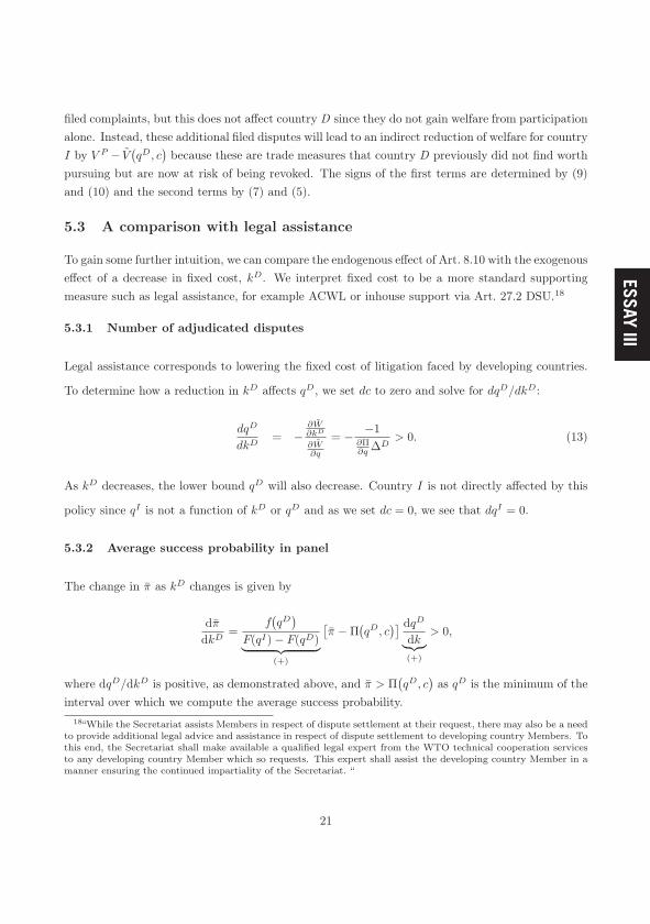
ESSAY III

The reason for this result is that, as c decreases both qD and qI will decrease which means thatF(qI)

and F(qD

)also decrease. Accordingly, the change in F (qI)−F (qD) is ambiguous, provided

we do not know the effect sizes. The effect on the integral is likewise ambiguous as it will dependon the unknown distribution of q around qI and qD. We draw the conclusion that subsidizingpreferential judges have ambiguous effects on the average success probability.


Lastly, we analyse welfare changes to evaluate if developing countries are better off with thesesupporting measures in place. For this purpose, we define the total expected welfare for country Dand country I, respectively:

E [W ] = WPF (qD) +

∫ qI

qDf(q) W(q; ·) dq +WL

[1− F (qI)

](11)

E [V ] = V PF (qD) +

∫ qI

qDf(q) V(q; ·) dq + V L

[1− F (qI)

](12)

Welfare stems from three sources in equations (11) and (12): The first term captures trade measuresthat are not challenged, the second term represents trade measures that are adjudicated and thethird term captures trade measures that are challenged but not defended.

The net welfare effects for country D when subsidizing preferential judges are therefore givenby

dE [W ]

dc=

∫ qI

qDf (q)

∂W(q; ·)∂c︸︷︷︸(−)

dq + f(qI) (

W(qI ; ·)−WL

)︸︷︷︸

(−)

dqI

dc︸︷︷︸(+)

< 0,

and for country I by

dE [V ]

dc=

∫ qI

qDf (q)

∂V(q; ·)∂c︸︷︷︸(+)

dq + f(qD

) (V P − V

(qD; ·)

)︸︷︷︸

(+)

dqD

dc︸︷︷︸(+)

> 0.

Thus, in contrast to the effect on observable outcomes, the welfare effect can be unambiguouslyestablished to be welfare-enhancing for country D and welfare-reducing for country I. For a givenset of disputes, there is a direct welfare effect, ∂W/∂c < 0, when reducing c for country D and alsoan indirect effect when country I settles more disputes without adjudication; contributing to anincrease in the number of disputes won by country D. As we lowers c, there is also an increase in

20

filed complaints, but this does not affect country D since they do not gain welfare from participationalone. Instead, these additional filed disputes will lead to an indirect reduction of welfare for countryI by V P − V

(qD, c

)because these are trade measures that country D previously did not find worth

pursuing but are now at risk of being revoked. The signs of the first terms are determined by (9)and (10) and the second terms by (7) and (5).

5.3 A comparison with legal assistance

To gain some further intuition, we can compare the endogenous effect of Art. 8.10 with the exogenouseffect of a decrease in fixed cost, kD. We interpret fixed cost to be a more standard supportingmeasure such as legal assistance, for example ACWL or inhouse support via Art. 27.2 DSU.18


Legal assistance corresponds to lowering the fixed cost of litigation faced by developing countries.

To determine how a reduction in kD affects qD, we set dc to zero and solve for dqD/dkD:

dqD

dkD= −

∂W∂kD

∂W∂q

= − −1∂Π∂q Δ

D> 0. (13)

As kD decreases, the lower bound qD will also decrease. Country I is not directly affected by this

policy since qI is not a function of kD or qD and as we set dc = 0, we see that dqI = 0.


The change in π as kD changes is given by

dπ

dkD=

f(qD

)F(qI)− F(qD)︸︷︷︸

(+)

[π −Π

(qD, c

)] dqDdk︸︷︷︸(+)

> 0,

where dqD/dkD is positive, as demonstrated above, and π > Π(qD, c

)as qD is the minimum of the

interval over which we compute the average success probability.18“While the Secretariat assists Members in respect of dispute settlement at their request, there may also be a need

to provide additional legal advice and assistance in respect of dispute settlement to developing country Members. Tothis end, the Secretariat shall make available a qualified legal expert from the WTO technical cooperation servicesto any developing country Member which so requests. This expert shall assist the developing country Member in amanner ensuring the continued impartiality of the Secretariat. “

21


The net welfare effect for country D when lowering kD is given by:

dE [W ]

dkD=

∫ qI

qDf(q)

∂W(q; ·)∂kD︸︷︷︸(−)

dq < 0,

and for country I bydE [V ]

dkD= f

(qD

) (V P − V

(qD; ·)

)︸︷︷︸

(+)

dqD

dkD︸︷︷︸(+)

> 0.

The signs of all the terms were determined by (7), (5) and (13).

Observation 1.

We first note that both Art. 8.10 and legal assistance encourage developing countries to file morecomplaints, meaning that they are more willing to pursue disputes with lower marginal benefits. Butsince a decrease in kD only affects the reservation point for developing countries while qI remainsunchanged, the dispute interval widens. Thus, when developing countries file more complaints, thenumber of adjudicated disputes will increase directly, which in turn may either decrease of increasethe total number of adjudicated disputes depending on the probability distribution around qI . Incomparison, a reduction in variable litigation cost will instead make industrialized countries moreinclined to settle as their reservation point qI decreases. Finally, as fixed litigation cost decreases,the additional disputes pursued by developing countries will be of lower quality, which will directlylower the average success probability, unlike the more inconclusive result for Art. 8.10.

Observation 2.

The overall effects show that both supporting measures are welfare-enhancing for country D andwelfare-reducing for country I. There are two sources for these welfare gains: first, when litigationcosts are reduced, there is a direct increase in welfare; second, when subsidizing preferential judges,country I will now choose to settle previously contested disputes. In contrast, there is a direct nega-tive effect on industrialized countries’ welfare and both supporting measures are welfare decreasingbecause fewer disputes are now settled to the advantage of industrialized countries. Comparingthese results with the previously derived policy effects reveal that the number of adjudicated dis-putes and success rates do not reflect the full impact of the supporting measures. Thus, the benefit

22

of the supporting measures for developing countries cannot be inferred from observed participationfrequency or average success probability.

6 Concluding remarks

We developed a theoretical framework for the purpose of explaining the observed relationship bet-ween developing-country judges and developing-country success rate in panel adjudication. Giventhe existence of the SDT provision Art. 8.10 of the DSU, there seems to be an a priori belief thatincluding developing-country judges on the panel will benefit developing countries. However, thereis little evidence of such benefits, thus, Art. 8.10 seems to be mainly be based on a common be-lief. We make a first attempt at evaluating the a priori belief of Art. 8.10 by empirically examinewhether developing-country judges have a positive impact on success rate for developing countries.Initially, it appeared as developing countries lost more claims the more developing-country judgeswere appointed, ostensibly refuting the presumed benefit of Art. 8.10. However, this counter in-tuitive result can be consistent with the belief that developing-country judges are advantageousfor developing countries if the data exhibits a Yule-Simpson’s paradox—a statistical phenomenonwhere a relationship can be reversed due to a moderating variable. To be able to explain the empi-rical observation given that the a priori belief is true, we developed a simple theoretical frameworkthat outlines the decision to participate by both parties, where the developing country optimizedpanel composition with developing-country judges. This approach allowed us to understand therole of the moderating variable and the underlying mechanism. Our model explains the paradox asfollows: if there is a presumption that developing-country judges can increase the success rate fordeveloping countries then such judges will be more valuable in weaker cases. For that reason, wewill observe more such judges on panels that handle low-quality disputes. However, these judgeswon’t be able to turn around a bad case, thus, the negative relationship between developing-countryjudges and the developing-country success rate that we found in the data is therefore explained bymeans of selection: developing countries that bring weak cases to adjudication will promote moredeveloping-country judges onto the panel, but simultaneously, they will lose more claims due to thepoor legal merits of the case.

Apart from our main purpose to explain the observed data, we also conducted comparativestatics analysis of Art. 8.10 in regards to average success rate, participation rate and welfare effects.We show that reducing dispute costs increase the number of complaints filed by developing countries,however, this increase may not always be reflected in the number of adjudications. As it becomeseasier for developing countries to promote developing-country judges, it becomes relatively moredifficult for industrialized countries to win in adjudication and thus, industrialized countries requirea higher marginal benefit to adjudicate. This implies that after the policy reform, marginal disputes,that were previously adjudicated, are now settled. Subsidizing preferential judges implies two effects

23

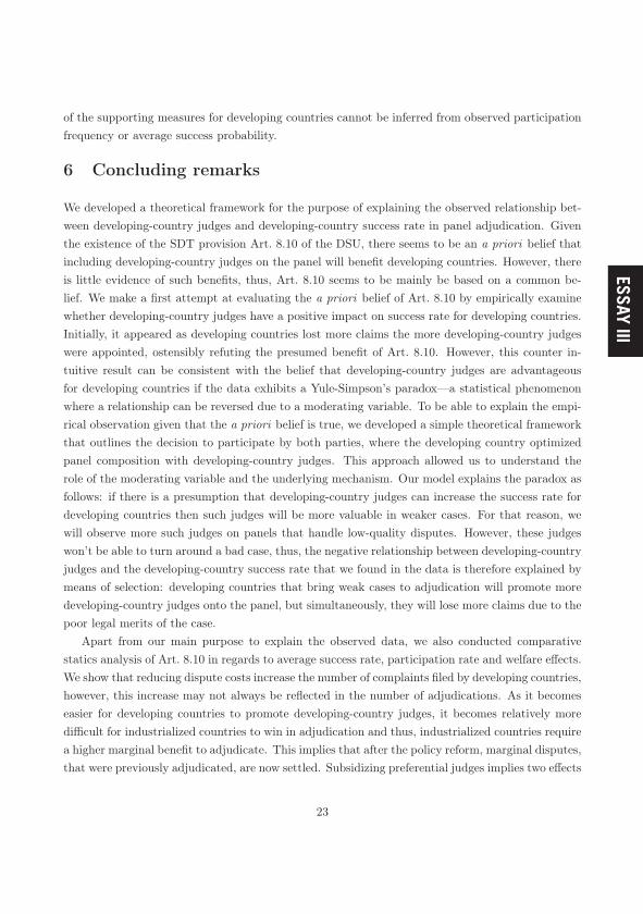
ESSAY III


The net welfare effect for country D when lowering kD is given by:

dE [W ]

dkD=

∫ qI

qDf(q)

∂W(q; ·)∂kD︸︷︷︸(−)

dq < 0,

and for country I bydE [V ]

dkD= f

(qD

) (V P − V

(qD; ·)

)︸︷︷︸

(+)

dqD

dkD︸︷︷︸(+)

> 0.

The signs of all the terms were determined by (7), (5) and (13).

Observation 1.

We first note that both Art. 8.10 and legal assistance encourage developing countries to file morecomplaints, meaning that they are more willing to pursue disputes with lower marginal benefits. Butsince a decrease in kD only affects the reservation point for developing countries while qI remainsunchanged, the dispute interval widens. Thus, when developing countries file more complaints, thenumber of adjudicated disputes will increase directly, which in turn may either decrease of increasethe total number of adjudicated disputes depending on the probability distribution around qI . Incomparison, a reduction in variable litigation cost will instead make industrialized countries moreinclined to settle as their reservation point qI decreases. Finally, as fixed litigation cost decreases,the additional disputes pursued by developing countries will be of lower quality, which will directlylower the average success probability, unlike the more inconclusive result for Art. 8.10.

Observation 2.

The overall effects show that both supporting measures are welfare-enhancing for country D andwelfare-reducing for country I. There are two sources for these welfare gains: first, when litigationcosts are reduced, there is a direct increase in welfare; second, when subsidizing preferential judges,country I will now choose to settle previously contested disputes. In contrast, there is a direct nega-tive effect on industrialized countries’ welfare and both supporting measures are welfare decreasingbecause fewer disputes are now settled to the advantage of industrialized countries. Comparingthese results with the previously derived policy effects reveal that the number of adjudicated dis-putes and success rates do not reflect the full impact of the supporting measures. Thus, the benefit

22

of the supporting measures for developing countries cannot be inferred from observed participationfrequency or average success probability.


We developed a theoretical framework for the purpose of explaining the observed relationship bet-ween developing-country judges and developing-country success rate in panel adjudication. Giventhe existence of the SDT provision Art. 8.10 of the DSU, there seems to be an a priori belief thatincluding developing-country judges on the panel will benefit developing countries. However, thereis little evidence of such benefits, thus, Art. 8.10 seems to be mainly be based on a common be-lief. We make a first attempt at evaluating the a priori belief of Art. 8.10 by empirically examinewhether developing-country judges have a positive impact on success rate for developing countries.Initially, it appeared as developing countries lost more claims the more developing-country judgeswere appointed, ostensibly refuting the presumed benefit of Art. 8.10. However, this counter in-tuitive result can be consistent with the belief that developing-country judges are advantageousfor developing countries if the data exhibits a Yule-Simpson’s paradox—a statistical phenomenonwhere a relationship can be reversed due to a moderating variable. To be able to explain the empi-rical observation given that the a priori belief is true, we developed a simple theoretical frameworkthat outlines the decision to participate by both parties, where the developing country optimizedpanel composition with developing-country judges. This approach allowed us to understand therole of the moderating variable and the underlying mechanism. Our model explains the paradox asfollows: if there is a presumption that developing-country judges can increase the success rate fordeveloping countries then such judges will be more valuable in weaker cases. For that reason, wewill observe more such judges on panels that handle low-quality disputes. However, these judgeswon’t be able to turn around a bad case, thus, the negative relationship between developing-countryjudges and the developing-country success rate that we found in the data is therefore explained bymeans of selection: developing countries that bring weak cases to adjudication will promote moredeveloping-country judges onto the panel, but simultaneously, they will lose more claims due to thepoor legal merits of the case.

Apart from our main purpose to explain the observed data, we also conducted comparativestatics analysis of Art. 8.10 in regards to average success rate, participation rate and welfare effects.We show that reducing dispute costs increase the number of complaints filed by developing countries,however, this increase may not always be reflected in the number of adjudications. As it becomeseasier for developing countries to promote developing-country judges, it becomes relatively moredifficult for industrialized countries to win in adjudication and thus, industrialized countries requirea higher marginal benefit to adjudicate. This implies that after the policy reform, marginal disputes,that were previously adjudicated, are now settled. Subsidizing preferential judges implies two effects

23

for developing countries: first, they will file more disputes than they otherwise would have doneand second, they will win more disputes without adjudication. Furthermore, a consequence of anincrease or decrease in the number of adjudications will be a subsequent change in average successprobability because the developing countries will file more disputes as dispute costs are reduced, butthese marginal disputes will be of lower quality thereby lowering the average success probability.By the same token, there are ambiguous effects on the frequency of adjudication, which impliessimilarly ambiguous effects on average success probability, thus demonstrating that a decrease inaverage success probability is not indicative of a bad policy, but may in fact indicate the opposite.Despite the somewhat mixed policy effects in our model, the welfare effects are unambiguouslypositive for developing countries, given that those welfare gains arose from lower dispute costs andfrom successful complaints since our model does not take into account any welfare gains that stemfrom participation alone.

References

Beshkar, M. (2010). Trade skirmishes safeguards: A theory of the WTO dispute settlement process.

Journal of International Economics 82 (1), 35–48.

Bohanes, J. and F. Garza (2012). Going beyond stereotypes: participation of developing countries

in WTO dispute settlement. Trade Law & Development 4 (1), 45–128.

Bourgeois, J. H. J. (2001). Some Reflections on the WTO Dispute Settlement System from a

practitioner’s perspective. Journal of International Economic Law 3, 145–154.

Bown, C. P. and B. M. Hoekman (2005). WTO dispute settlement and the missing developing

country cases : engaging the private sector. 8 (4), 861–890.

Bown, C. P. and R. McCulloch (2010). Developing countries, dispute settlement, and the Advisory

Centre on WTO Law. The Journal of International Trade & Economic Development 19 (1),

33–63.

Davis, C. L. and S. B. Bermeo (2009). Who Files? Developing Country Participation in

GATT/WTO Adjudication. The Journal of Politics 71 (03), 1033.

Goodman, A. T. (2013, June). Kitchen Sink Litigation Clogs the Judicial Pipeline. Retrieved at

https://www.law360.com/articles/452235/.

24

Guzman, A. T. and B. a. Simmons (2005). Power Plays and Capacity Constraints: The Selection of

Defendants in World Trade Organization Disputes. The Journal of Legal Studies 34 (2), 557–598.

Hoekman, B., H. Horn, and P. C. Mavroidis (2009). Winners and Losers in the Panel Stage of

the WTO Dispute Settlement System. In J. P. Trachtman and C. Thomas (Eds.), Developing

Countries in the WTO Legal System, Number April, Chapter 8, pp. 1–21. Oxford University

Press.

Horn, H. (2011). The burden of proof in trade disputes and the environment. Journal of Environ-

mental Economics and Management 62 (1), 15–29.

Horn, H., L. Johannesson, and P. C. Mavroidis (2011). The WTO dispute settlement system

1995-2010: Some descriptive statistics. Journal of World Trade 45 (6), 1107–1138.

Lindley, D. V. and M. R. Novick (1981). The role of exchangeability in inference. The Annals of

Statistics 9 (1), 45–58.

Mitchell, K. M. W. (2013). Developing country success in WTO disputes. Journal of World

Trade 47 (1), 77–104.

Pearl, J. (2009). Causality: Models, Reasoning and Inference (2nd ed.). New York, NY, USA:

Cambridge University Press.

Pearl, J. (2014). Understanding Simpson’s Paradox. The American Statistician 68 (1), 8–13.

Shoyer, A. W. (2003). Panel selection in WTO dispute settlement proceedings. Journal of Inter-

national Economic Law 6 (1), 203–209.

25

ESSAY III

for developing countries: first, they will file more disputes than they otherwise would have doneand second, they will win more disputes without adjudication. Furthermore, a consequence of anincrease or decrease in the number of adjudications will be a subsequent change in average successprobability because the developing countries will file more disputes as dispute costs are reduced, butthese marginal disputes will be of lower quality thereby lowering the average success probability.By the same token, there are ambiguous effects on the frequency of adjudication, which impliessimilarly ambiguous effects on average success probability, thus demonstrating that a decrease inaverage success probability is not indicative of a bad policy, but may in fact indicate the opposite.Despite the somewhat mixed policy effects in our model, the welfare effects are unambiguouslypositive for developing countries, given that those welfare gains arose from lower dispute costs andfrom successful complaints since our model does not take into account any welfare gains that stemfrom participation alone.

References

Beshkar, M. (2010). Trade skirmishes safeguards: A theory of the WTO dispute settlement process.

Journal of International Economics 82 (1), 35–48.

Bohanes, J. and F. Garza (2012). Going beyond stereotypes: participation of developing countries

in WTO dispute settlement. Trade Law & Development 4 (1), 45–128.

Bourgeois, J. H. J. (2001). Some Reflections on the WTO Dispute Settlement System from a

practitioner’s perspective. Journal of International Economic Law 3, 145–154.

Bown, C. P. and B. M. Hoekman (2005). WTO dispute settlement and the missing developing

country cases : engaging the private sector. 8 (4), 861–890.

Bown, C. P. and R. McCulloch (2010). Developing countries, dispute settlement, and the Advisory

Centre on WTO Law. The Journal of International Trade & Economic Development 19 (1),

33–63.

Davis, C. L. and S. B. Bermeo (2009). Who Files? Developing Country Participation in

GATT/WTO Adjudication. The Journal of Politics 71 (03), 1033.

Goodman, A. T. (2013, June). Kitchen Sink Litigation Clogs the Judicial Pipeline. Retrieved at

https://www.law360.com/articles/452235/.

24

Guzman, A. T. and B. a. Simmons (2005). Power Plays and Capacity Constraints: The Selection of

Defendants in World Trade Organization Disputes. The Journal of Legal Studies 34 (2), 557–598.

Hoekman, B., H. Horn, and P. C. Mavroidis (2009). Winners and Losers in the Panel Stage of

the WTO Dispute Settlement System. In J. P. Trachtman and C. Thomas (Eds.), Developing

Countries in the WTO Legal System, Number April, Chapter 8, pp. 1–21. Oxford University

Press.

Horn, H. (2011). The burden of proof in trade disputes and the environment. Journal of Environ-

mental Economics and Management 62 (1), 15–29.

Horn, H., L. Johannesson, and P. C. Mavroidis (2011). The WTO dispute settlement system

1995-2010: Some descriptive statistics. Journal of World Trade 45 (6), 1107–1138.

Lindley, D. V. and M. R. Novick (1981). The role of exchangeability in inference. The Annals of

Statistics 9 (1), 45–58.

Mitchell, K. M. W. (2013). Developing country success in WTO disputes. Journal of World

Trade 47 (1), 77–104.

Pearl, J. (2009). Causality: Models, Reasoning and Inference (2nd ed.). New York, NY, USA:

Cambridge University Press.

Pearl, J. (2014). Understanding Simpson’s Paradox. The American Statistician 68 (1), 8–13.

Shoyer, A. W. (2003). Panel selection in WTO dispute settlement proceedings. Journal of Inter-

national Economic Law 6 (1), 203–209.

25

A Stylized facts

Figure 1: Success rate by developing country complainants

0

.2

.4

.6

.8

1

Aver

age

succ

ess r

ate

0 1 2 3Developing country complainants, only

B Developing countries in adjudication

B.1 Country classification

There is no official country classification system within the WTO; instead a country self-selects

into one of two categories: developing country or industrialized country. Countries that are classified

as least-developed by the United Nations will automatically be recognized as such in the WTO.

The self-imposed development status does not, however, automatically entitle a member to the use

of SDT privileges, as other members can contest their status. Bohanes and Garza (2012) notes,

however, that in practice, development status is rarely contested. Considering that developing

countries are a far more diverse group than industrialized countries, the rough country classification

of the WTO may seem questionable. Horn (2011) notes this and instead divides WTO Members

26

into five income categories: least-developed, developing, BIC (Brazil, India and China), developed

and G2 (US and EU). Separating out BIC acknowledges that these countries are usually considered

emerging markets and hence not as economically constrained as we might expect from developing

countries. (Together with Russia, they are part of the country group usually recognized as BRIC.

However, Russia only became a member in 2012 and is therefore not yet included in these data.)

For the rest of the developing country group, no relevant country (i.e., countries that have been

involved in panel adjudication) have graduated to developed country status within this time period,

except for South Korea. It proclaimed itself to be a developing country when joining the WTO in

1995 and its official status has not changed since then, even though it graduated to industrialized

country status in 1997. We therefore categorized South Korea as an industrialized country. We

have otherwise adhered to the self-selected status, following Horn (2011). The same classification

scheme was used to determine the geographical background of the judges.

As complainant Freq. As respondent Freq.Antigua and Barbuda 1 Argentina 7Argentina 2 Brazil 2Brazil 11 Chile 2Chile 1 China 15China 6 India 7Chinese Taipei 1 Indonesia 4Costa Rica 1 Mexico 5Ecuador 2 Philippines 2Guatemala 1 Thailand 1Honduras 1 Turkey 1India 9Indonesia 3Malaysia 1Mexico 5Pakistan 2Peru 1Thailand 6Venezuela 1Viet Nam 2

Total 57 Total 46

Table 1: Developing countries in adjudication against industrialized countries

27

ESSAY III

A Stylized facts

Figure 1: Success rate by developing country complainants

0

.2

.4

.6

.8

1

Aver

age

succ

ess r

ate

0 1 2 3Developing country complainants, only

B Developing countries in adjudication

B.1 Country classification

There is no official country classification system within the WTO; instead a country self-selects

into one of two categories: developing country or industrialized country. Countries that are classified

as least-developed by the United Nations will automatically be recognized as such in the WTO.

The self-imposed development status does not, however, automatically entitle a member to the use

of SDT privileges, as other members can contest their status. Bohanes and Garza (2012) notes,

however, that in practice, development status is rarely contested. Considering that developing

countries are a far more diverse group than industrialized countries, the rough country classification

of the WTO may seem questionable. Horn (2011) notes this and instead divides WTO Members

26

into five income categories: least-developed, developing, BIC (Brazil, India and China), developed

and G2 (US and EU). Separating out BIC acknowledges that these countries are usually considered

emerging markets and hence not as economically constrained as we might expect from developing

countries. (Together with Russia, they are part of the country group usually recognized as BRIC.

However, Russia only became a member in 2012 and is therefore not yet included in these data.)

For the rest of the developing country group, no relevant country (i.e., countries that have been

involved in panel adjudication) have graduated to developed country status within this time period,

except for South Korea. It proclaimed itself to be a developing country when joining the WTO in

1995 and its official status has not changed since then, even though it graduated to industrialized

country status in 1997. We therefore categorized South Korea as an industrialized country. We

have otherwise adhered to the self-selected status, following Horn (2011). The same classification

scheme was used to determine the geographical background of the judges.

As complainant Freq. As respondent Freq.Antigua and Barbuda 1 Argentina 7Argentina 2 Brazil 2Brazil 11 Chile 2Chile 1 China 15China 6 India 7Chinese Taipei 1 Indonesia 4Costa Rica 1 Mexico 5Ecuador 2 Philippines 2Guatemala 1 Thailand 1Honduras 1 Turkey 1India 9Indonesia 3Malaysia 1Mexico 5Pakistan 2Peru 1Thailand 6Venezuela 1Viet Nam 2

Total 57 Total 46

Table 1: Developing countries in adjudication against industrialized countries

27

B.2 BIC countries

The benefit of developing-country judges is less apparent for the BIC country group compared

to other developing countries, as their legal capacity is closer to that of the richer members. Ne-

vertheless, they are still developing countries in many other respects, and therefore such expertise

may still prove valuable. In fact, India is a member of the ACWL. Figure suggests at least that

the BIC countries appear to behave as other developing countries with respect to our proposed

selection effect of developing-country judges.

0

.2

.4

.6

Suc

cess

rate

(Bra

zil,

Indi

a &

Chi

na)

0 1 2 3N=50

0

.2

.4

.6S

ucce

ss ra

te(d

evel

opin

g co

untri

es, e

xclu

ding

BIC

)

0 1 2 3N=53

Figure 2: Success rate and developing-country judges for BIC

B.3 Developing country complainant and respondent

It may be relevant to examine the outcomes conditional on whether the developing country is a

complainant or a respondent, to ensure that Figure 2 is not the result of compositional effects due

to complainant/respondent specific attributes.

28

Figure 3: Success rates for developing country complainants and respondents, by developing-countryjudges

0

.2

.4

.6

.8

Suc

cess

rate

(dev

elop

ing

coun

try c

ompl

aina

nt)

0 1 2N = 59

0

.1

.2

.3

Suc

cess

rate

(dev

elop

ing

coun

try re

sond

ent)

0 1 2 3N = 46

Figure 3 shows that the negative linear correlation with developing-country judges is present

regardless of whether the developing country is a complainant or a respondent. However, the

correlation is only significant (at the 5% significance level) for complainants. Respondents and

complainants could therefore differ in certain respects relating to the choice of developing-country

judges. However it is also likely that there are too few observations to discern any significant

differences. Respondents only had 5 disputes without any developing-country judges, while there

are 10 such disputes for complainants.

C Developing country as respondent

We show here how the model can be adapted to capture cases in which developing countries

are respondents. Recall, that the success probability function is developing-country specific, and

therefore it is defined as before: π = Π(q, n). Dispute quality q is also developing-country specific

and measures the legal merits of the case for developing countries. It will therefore result in the same

dispute interval. The timing and the payoffs, however, are changed. The payoffs that country I and

D receive if the trade measure goes unchallenged are V P and WP . If country I decides to launch a

29

ESSAY III

B.2 BIC countries

The benefit of developing-country judges is less apparent for the BIC country group compared

to other developing countries, as their legal capacity is closer to that of the richer members. Ne-

vertheless, they are still developing countries in many other respects, and therefore such expertise

may still prove valuable. In fact, India is a member of the ACWL. Figure suggests at least that

the BIC countries appear to behave as other developing countries with respect to our proposed

selection effect of developing-country judges.

0

.2

.4

.6

Suc

cess

rate

(Bra

zil,

Indi

a &

Chi

na)

0 1 2 3N=50

0

.2

.4

.6

Suc

cess

rate

(dev

elop

ing

coun

tries

, exc

ludi

ng B

IC)

0 1 2 3N=53

Figure 2: Success rate and developing-country judges for BIC

B.3 Developing country complainant and respondent

It may be relevant to examine the outcomes conditional on whether the developing country is a

complainant or a respondent, to ensure that Figure 2 is not the result of compositional effects due

to complainant/respondent specific attributes.

28

Figure 3: Success rates for developing country complainants and respondents, by developing-countryjudges

0

.2

.4

.6

.8

Suc

cess

rate

(dev

elop

ing

coun

try c

ompl

aina

nt)

0 1 2N = 59

0

.1

.2

.3

Suc

cess

rate

(dev

elop

ing

coun

try re

sond

ent)

0 1 2 3N = 46

Figure 3 shows that the negative linear correlation with developing-country judges is present

regardless of whether the developing country is a complainant or a respondent. However, the

correlation is only significant (at the 5% significance level) for complainants. Respondents and

complainants could therefore differ in certain respects relating to the choice of developing-country

judges. However it is also likely that there are too few observations to discern any significant

differences. Respondents only had 5 disputes without any developing-country judges, while there

are 10 such disputes for complainants.

C Developing country as respondent

We show here how the model can be adapted to capture cases in which developing countries

are respondents. Recall, that the success probability function is developing-country specific, and

therefore it is defined as before: π = Π(q, n). Dispute quality q is also developing-country specific

and measures the legal merits of the case for developing countries. It will therefore result in the same

dispute interval. The timing and the payoffs, however, are changed. The payoffs that country I and

D receive if the trade measure goes unchallenged are V P and WP . If country I decides to launch a

29

complaint that country D settles, then country I and D receive WL and V L respectively. A dispute

is only adjudicated if country I files a complaint that country D opposes; at that time country I

receives expected welfare V(q, n, kI

)and country D receives W

(q, n, kD, c

). The changed payoffs

imply the following indifference conditions V(qI) ≡ V P and W

(qD

) ≡ WL, which in turn means

that the intervals in which settlements take place have switched. That is, country D surrenders all

trade measures up to qD while country I refrains from making complaints for all disputes in the

interval 1− qI .

D Proof of proposition 1

Let c be sufficiently high that there are no developing-country judges on the panel. We then

have:

Π(qD, 0

)ΔD − kD +WP = WP

[1−Π

(qD, 0

)]ΔI − kI + V L = V L

Rearrange and divide both sides by ΔD and ΔI , respectively.

Π(qD

)= kD

ΔD ≡ γD

1−Π(qD

)= kI

ΔI ≡ γI .

As Π is monotonically increasing in q for the complainant, there exists an inverse function Π−1

such that

qD = Π−1(γD

)

qI = Π−1(1− γI

).

And, since Π is monotonically increasing in q, Π−1 is monotonically increasing in γ. Hence, for

γD < 1− γI , qD < qI , and there will be panels in equilibrium.

30

ESSAY IV

Efficiency gains and time-savings of permanent panels in the

WTO dispute settlement


1 Introduction

Although the success of the dispute settlement mechanism (DSM) of the World Trade Or-

ganization (WTO) has been received enthusiastically, it has also brought on new challenges

that have proved difficult to resolve. Issues such as increasingly time-consuming and com-

plex disputes have strained the capacity of the WTO and led to delays. The WTO has

long prided itself on prompt dispute resolutions, recognizing that excessive delays may force

countries to find alternative solutions, which would, in the long-run, undermine the legi-

timacy of the DSM. Recent increases in the number of appeals (88% of all panel reports

were appealed in 2016) prompted the current chairman of the Appellate Body (AB) Ujal

Singh Bhatia, to explicitly address the problem of delays in the DSM.1 He explained the

situation and the consequences if the problem remains unresolved as: “When delays in

WTO dispute resolution become the norm, they cast doubt on the value of the WTO’s

rules-oriented system itself. An erosion of trust in this system can lead to the re-emergence

of power orientation in international trade policy”. Apart from legitimacy concerns, time-

liness is also a serious economic issue since delays in rulings also delay the removal of the∗Research Institute of Industrial Economics, Box 55665, SE-102 15 Stockholm and Örebro University,

Sweden. E-mail: [email protected]. For valuable comments, I would like to express my gratitudeto Henrik Horn at IFN, Magnus Lodefalk and Dan Johansson at Örebro University, Hildegunn KyvikNordås at the OECD, and Jonas Björnerstedt at Södertörn University. I gratefully acknowledges financialsupport from the Jan Wallander and Tom Hedelius Foundation and the Marianne and Marcus WallenbergFoundation.

1The event in question was a presentation of the Appellate Body’s 2016 Annual Report.https://www.wto.org/english/news_e/news17_e/ab_08jun17_e.htm

1

ESSAY IV

Efficiency gains and time-savings of permanent panels in the

WTO dispute settlement


1 Introduction

Although the success of the dispute settlement mechanism (DSM) of the World Trade Or-

ganization (WTO) has been received enthusiastically, it has also brought on new challenges

that have proved difficult to resolve. Issues such as increasingly time-consuming and com-

plex disputes have strained the capacity of the WTO and led to delays. The WTO has

long prided itself on prompt dispute resolutions, recognizing that excessive delays may force

countries to find alternative solutions, which would, in the long-run, undermine the legi-

timacy of the DSM. Recent increases in the number of appeals (88% of all panel reports

were appealed in 2016) prompted the current chairman of the Appellate Body (AB) Ujal

Singh Bhatia, to explicitly address the problem of delays in the DSM.1 He explained the

situation and the consequences if the problem remains unresolved as: “When delays in

WTO dispute resolution become the norm, they cast doubt on the value of the WTO’s

rules-oriented system itself. An erosion of trust in this system can lead to the re-emergence

of power orientation in international trade policy”. Apart from legitimacy concerns, time-

liness is also a serious economic issue since delays in rulings also delay the removal of the∗Research Institute of Industrial Economics, Box 55665, SE-102 15 Stockholm and Örebro University,

Sweden. E-mail: [email protected]. For valuable comments, I would like to express my gratitudeto Henrik Horn at IFN, Magnus Lodefalk and Dan Johansson at Örebro University, Hildegunn KyvikNordås at the OECD, and Jonas Björnerstedt at Södertörn University. I gratefully acknowledges financialsupport from the Jan Wallander and Tom Hedelius Foundation and the Marianne and Marcus WallenbergFoundation.

1The event in question was a presentation of the Appellate Body’s 2016 Annual Report.https://www.wto.org/english/news_e/news17_e/ab_08jun17_e.htm

1

illegal trade barriers. And the DSM does not award retro-active compensation in case of a

violation.

Canada voiced concern over delays in a Dispute Settlement Body (DSB) meeting2 in

relation to dispute DS 384, stating that they had faced numerous delays that had unduly

prolonged the economic burden on the Canadian economy. Korea expressed a similar sen-

timent in 20153 when they acted as a complainant in a dispute concerning anti-dumping

measures by the US against certain Korean steel products (DS 488). They argued that

excessive delays resulted in losses of ten million US dollars a month for Korean firms, which

would cause a substantial number of job losses and failed businesses. The statutory dead-

line of panel proceedings is six months, but the average length of a panel process is around

15 months. This implies that an additional nine months are added to the proceedings, and

in the case of the Korean anti-dumping dispute, an additional loss of 90 million US dol-

lars. They further expounded on the detrimental consequences of protracted adjudications:

“Long delays created perverse incentives by lowering the cost of adopting and maintaining

WTO-inconsistent measures. Interest groups seeking protection would pressure Members

to adopt these measures, insisting rightly, that they would not be subject to review by the

WTO for years. Members could therefore expect more protectionist measures, and more,

not less, disputes being brought to the WTO”. In summary, it is evident that undue delays

cause economic harm and that the DSM will be weakened if the problem is allowed to per-

sist, forcing countries to seek alternative solutions for their trade skirmishes, alternatives

that may be less transparent and based more on negotiating power.

The capacity constraint of the DSM clearly requires a comprehensive approach, where

all the different stages are investigated to improve overall timeliness. One reform in that

direction may be to install permanent panels. The idea of permanent panels, instead of the

current regime of ad hoc panels, has been a recurring subject since panels were introduced

into the GATT (Jackson, 1979; Tuthill et al., 1985). Various WTO members, most notably

the EU (2002)4 and academics, such as Hudec (1999), Davey (2003), Bourgeois (2003),

Cottier (2003) and Busch and Pelc (2009), have expressed support for some variant of a

permanent panel, as it will automatically save time by eliminating the, at times protrac-2WT/DSB/M/3623WT/DSB/M/3674TN/DS/W/1

2

ted selection process. Furthermore, it has also been argued that a permanent panel could

increase efficiency and quality in rulings as panelists will be more experienced than ad hoc

panelists (for example Busch and Pelc, 2009). However, political apprehension, especially

from the US (Cottier, 2003) has effectively made such proposals moot. As Bourgeois (2003)

notes, “the underlying tension lies between legitimacy and efficiency”, where scholars and

trade experts give priority to the latter, while the politicians stress the former, and for

the WTO, an inter-governmental body, the weight of legitimacy lies heavy in the debate.

However, if the problem of delays becomes a bigger and bigger threat to the legitimacy of

the DSM, there may be cause to re-consider the importance of efficiency vis-à-vis legiti-

macy. This paper contributes to this discussion by analyzing certain panel features that

characterize a permanent panel, namely, the panelists’ experience and whether a prior work

relationship between the panelists facilitates their deliberations. We examine how these fac-

tors contribute to the time it takes to issue a panel report, as used in previous studies, but

also a panel’s efficiency in examining claims.

The results show that the combined experience of the panel does not reduce the time

it takes to issue a report, as found in Horn (2013), but it slightly decreases efficiency. One

reason why more experience leads to longer panel deliberations could be selection effects.

That is, more experienced panelists are appointed in more complicated cases, which in

turn takes longer to complete. We find, however, that panelists that work with previous co-

panelists can reduce the time by around 30 days, a result that weighs in favour of permanent

panels.

The rest of the paper is organized as follows. Section 2 discusses the arguments for and

against permanent panels and the expected consequences. Section 3 describes the data,

variables and method, concluding with descriptive statistics. Section 4 characterizes the

institutional setting in which the disputes are examined. Section 5 presents the results of

the analysis, with a short comment on robustness. Section 6 concludes with a discussion.

2 Permanent or ad hoc panels

A constitutive argument against permanent panels has been that an ad hoc panel embodies

the spirit of the WTO as a member-driven organisation. Nonetheless, it has not gone

unnoticed that the majority, around 66% of all panels between 1995–2014, have actually

3

ESSAY IV

illegal trade barriers. And the DSM does not award retro-active compensation in case of a

violation.

Canada voiced concern over delays in a Dispute Settlement Body (DSB) meeting2 in

relation to dispute DS 384, stating that they had faced numerous delays that had unduly

prolonged the economic burden on the Canadian economy. Korea expressed a similar sen-

timent in 20153 when they acted as a complainant in a dispute concerning anti-dumping

measures by the US against certain Korean steel products (DS 488). They argued that

excessive delays resulted in losses of ten million US dollars a month for Korean firms, which

would cause a substantial number of job losses and failed businesses. The statutory dead-

line of panel proceedings is six months, but the average length of a panel process is around

15 months. This implies that an additional nine months are added to the proceedings, and

in the case of the Korean anti-dumping dispute, an additional loss of 90 million US dol-

lars. They further expounded on the detrimental consequences of protracted adjudications:

“Long delays created perverse incentives by lowering the cost of adopting and maintaining

WTO-inconsistent measures. Interest groups seeking protection would pressure Members

to adopt these measures, insisting rightly, that they would not be subject to review by the

WTO for years. Members could therefore expect more protectionist measures, and more,

not less, disputes being brought to the WTO”. In summary, it is evident that undue delays

cause economic harm and that the DSM will be weakened if the problem is allowed to per-

sist, forcing countries to seek alternative solutions for their trade skirmishes, alternatives

that may be less transparent and based more on negotiating power.

The capacity constraint of the DSM clearly requires a comprehensive approach, where

all the different stages are investigated to improve overall timeliness. One reform in that

direction may be to install permanent panels. The idea of permanent panels, instead of the

current regime of ad hoc panels, has been a recurring subject since panels were introduced

into the GATT (Jackson, 1979; Tuthill et al., 1985). Various WTO members, most notably

the EU (2002)4 and academics, such as Hudec (1999), Davey (2003), Bourgeois (2003),

Cottier (2003) and Busch and Pelc (2009), have expressed support for some variant of a

permanent panel, as it will automatically save time by eliminating the, at times protrac-2WT/DSB/M/3623WT/DSB/M/3674TN/DS/W/1

2

ted selection process. Furthermore, it has also been argued that a permanent panel could

increase efficiency and quality in rulings as panelists will be more experienced than ad hoc

panelists (for example Busch and Pelc, 2009). However, political apprehension, especially

from the US (Cottier, 2003) has effectively made such proposals moot. As Bourgeois (2003)

notes, “the underlying tension lies between legitimacy and efficiency”, where scholars and

trade experts give priority to the latter, while the politicians stress the former, and for

the WTO, an inter-governmental body, the weight of legitimacy lies heavy in the debate.

However, if the problem of delays becomes a bigger and bigger threat to the legitimacy of

the DSM, there may be cause to re-consider the importance of efficiency vis-à-vis legiti-

macy. This paper contributes to this discussion by analyzing certain panel features that

characterize a permanent panel, namely, the panelists’ experience and whether a prior work

relationship between the panelists facilitates their deliberations. We examine how these fac-

tors contribute to the time it takes to issue a panel report, as used in previous studies, but

also a panel’s efficiency in examining claims.

The results show that the combined experience of the panel does not reduce the time

it takes to issue a report, as found in Horn (2013), but it slightly decreases efficiency. One

reason why more experience leads to longer panel deliberations could be selection effects.

That is, more experienced panelists are appointed in more complicated cases, which in

turn takes longer to complete. We find, however, that panelists that work with previous co-

panelists can reduce the time by around 30 days, a result that weighs in favour of permanent

panels.

The rest of the paper is organized as follows. Section 2 discusses the arguments for and

against permanent panels and the expected consequences. Section 3 describes the data,

variables and method, concluding with descriptive statistics. Section 4 characterizes the

institutional setting in which the disputes are examined. Section 5 presents the results of

the analysis, with a short comment on robustness. Section 6 concludes with a discussion.

2 Permanent or ad hoc panels

A constitutive argument against permanent panels has been that an ad hoc panel embodies

the spirit of the WTO as a member-driven organisation. Nonetheless, it has not gone

unnoticed that the majority, around 66% of all panels between 1995–2014, have actually

3

been composed by the Director-General (DG) together with the Secretariat, and not by

the parties to the dispute; a trend that seem to have grown over time. One reason that

panel composition has been increasingly referred to the DG could be related to increased

complexity. Horn (2013) examines the determinants of time required to issue panel reports,

and he shows that panels that were appointed by the DG take longer to complete a panel

report compared to panels that were composed by the parties. This may indicate that the

DG is more often consulted in politically sensitive disputes.

One of the strongest arguments in favour of a permanent panel is that more experienced

panelists will increase the quality of the panel report, which will reduce the number of

reversals by the AB. Busch and Pelc (2009) examined this claim and found that, only

the experience of the chair significantly reduced the probability of the AB overturning a

ruling. This supports a type of mixed panel suggested by Cottier (2003), with permanent

chairs and ad hoc panelists. Horn (2013) also finds that the experience of panelists does

not facilitate the timeliness of a panel report, a result that further weakens the argument

for permanent panels. Additionally, he finds that a larger body of case law, which should

simplify the work, had no impact on time.

Another argument against permanent panels has been the lost opportunity for sociali-

zation for ad hoc panelists (Davey, 2003). The introduction of the DSM to hundreds of such

panelists may prove productive in the long-term for the reputation of the system. However,

the flip-side of this argument, and a feature of permanent panels, is the fact that the same

people will work together repeatedly and form closer work relationships compared to the

panelists that are selected ad hoc. It is entirely possible that such an arrangement would

improve work flow and save time.

3 Data and analysis

Data for this study is collected, mainly, from the publicly available “WTO dispute settlement

database”, originally compiled by Henrik Horn and Petros C. Mavroidis. It includes all

initiated disputes from 1995 to 2015.5 For descriptive statistics, we also use an institutional

variable—annual number of regular staff at the WTO Secretariat—that is found in the5The dataset can be freely downloaded here: http://globalgovernanceprogramme.eui.eu/wto-case-law-

project

4

WTO Annual Reports (1998–2015), subsection “Secretariat and the Budget”.

3.1 Variable description

The first outcome variable, time required to issue panel reports (hereafter “Duration”) was

calculated from the date of constitution of the panel to the date the panel circulated the

report. This includes the interim period, where the panel circulates the panel report only to

the affected parties. The statutory deadline is set at six months but Table 1 shows that the

average duration is usually over a year. Although duration may seem trivially correlated

with the number of claims, the relationship is not necessarily linear. It is reasonable to

assume that there are economies of scale in the legal analysis; that is, examining two claims

in a dispute does not take twice as long as examining a single claim. Panelists invest

considerable amount of effort for the first few claims as they familiarize themselves with

the facts and circumstances of the case; however, after this initial research, they are able

to complete the legal analysis for the subsequent claims more expeditiously.

For that reason, we also construct a second outcome, defined as days per invoked claim,

but each claim in a dispute is assigned different weights using the square root. This measure

is referred to as a square root equivalence scale. Let u be days between the constitution of

the panel and circulation of the panel report and cd be all cited claims in dispute d. We

compute equivalised duration per claim (henceforth Eq. days per claim), xd as:

xd =ud√cd

We interpret xd as follows: As the number of claims increases, the amount of time spent

on each claim decreases non-linearly. For example, a panel that has spent 100 days on

four claims will spend 50 Eq. days per claim (100/√4 = 50). One way to interpret this

variable is to imagine a panel that spends 50 days on two related claims concurrently, taking

advantage of economies of scale, instead of assuming the panelists spend 25 days on each

claim separately. An alternative definition to consider is to divide duration with unique

claims rather than all cited claims to better capture the true time spent on legal analysis.

However, this is exactly the type of situation that equivalisation should account for. (See

Appendix E for estimation results using alternative outcomes.)

The explanatory variables that we are particularly interested in are “experience”, “in-

5

ESSAY IV

been composed by the Director-General (DG) together with the Secretariat, and not by

the parties to the dispute; a trend that seem to have grown over time. One reason that

panel composition has been increasingly referred to the DG could be related to increased

complexity. Horn (2013) examines the determinants of time required to issue panel reports,

and he shows that panels that were appointed by the DG take longer to complete a panel

report compared to panels that were composed by the parties. This may indicate that the

DG is more often consulted in politically sensitive disputes.

One of the strongest arguments in favour of a permanent panel is that more experienced

panelists will increase the quality of the panel report, which will reduce the number of

reversals by the AB. Busch and Pelc (2009) examined this claim and found that, only

the experience of the chair significantly reduced the probability of the AB overturning a

ruling. This supports a type of mixed panel suggested by Cottier (2003), with permanent

chairs and ad hoc panelists. Horn (2013) also finds that the experience of panelists does

not facilitate the timeliness of a panel report, a result that further weakens the argument

for permanent panels. Additionally, he finds that a larger body of case law, which should

simplify the work, had no impact on time.

Another argument against permanent panels has been the lost opportunity for sociali-

zation for ad hoc panelists (Davey, 2003). The introduction of the DSM to hundreds of such

panelists may prove productive in the long-term for the reputation of the system. However,

the flip-side of this argument, and a feature of permanent panels, is the fact that the same

people will work together repeatedly and form closer work relationships compared to the

panelists that are selected ad hoc. It is entirely possible that such an arrangement would

improve work flow and save time.

3 Data and analysis

Data for this study is collected, mainly, from the publicly available “WTO dispute settlement

database”, originally compiled by Henrik Horn and Petros C. Mavroidis. It includes all

initiated disputes from 1995 to 2015.5 For descriptive statistics, we also use an institutional

variable—annual number of regular staff at the WTO Secretariat—that is found in the5The dataset can be freely downloaded here: http://globalgovernanceprogramme.eui.eu/wto-case-law-

project

4

WTO Annual Reports (1998–2015), subsection “Secretariat and the Budget”.

3.1 Variable description

The first outcome variable, time required to issue panel reports (hereafter “Duration”) was

calculated from the date of constitution of the panel to the date the panel circulated the

report. This includes the interim period, where the panel circulates the panel report only to

the affected parties. The statutory deadline is set at six months but Table 1 shows that the

average duration is usually over a year. Although duration may seem trivially correlated

with the number of claims, the relationship is not necessarily linear. It is reasonable to

assume that there are economies of scale in the legal analysis; that is, examining two claims

in a dispute does not take twice as long as examining a single claim. Panelists invest

considerable amount of effort for the first few claims as they familiarize themselves with

the facts and circumstances of the case; however, after this initial research, they are able

to complete the legal analysis for the subsequent claims more expeditiously.

For that reason, we also construct a second outcome, defined as days per invoked claim,

but each claim in a dispute is assigned different weights using the square root. This measure

is referred to as a square root equivalence scale. Let u be days between the constitution of

the panel and circulation of the panel report and cd be all cited claims in dispute d. We

compute equivalised duration per claim (henceforth Eq. days per claim), xd as:

xd =ud√cd

We interpret xd as follows: As the number of claims increases, the amount of time spent

on each claim decreases non-linearly. For example, a panel that has spent 100 days on

four claims will spend 50 Eq. days per claim (100/√4 = 50). One way to interpret this

variable is to imagine a panel that spends 50 days on two related claims concurrently, taking

advantage of economies of scale, instead of assuming the panelists spend 25 days on each

claim separately. An alternative definition to consider is to divide duration with unique

claims rather than all cited claims to better capture the true time spent on legal analysis.

However, this is exactly the type of situation that equivalisation should account for. (See

Appendix E for estimation results using alternative outcomes.)

The explanatory variables that we are particularly interested in are “experience”, “in-

5

crowd”, and to some extent also “case law”, since a rich case law may compensate low

experience to some degree. Experience is simply computed as the sum of all previous

panels that the current panelists have served on. We also include a squared-transformed

version. Along the same line, the variable “in-crowd” is the sum of previous panels that two

or more panelists in dispute d have served together on. Although being former co-panelists

may make it easier to work together and thus increase efficiency, it could also be entirely

possible that these previous interactions were unproductive and instead impede the process.

But since we can only observe previous interactions, we try to better capture positive effects

of established work relationships by including an interaction variable between the DG and

in-crowd. We hypothesize that the DG and Secretariat are better at selecting a panel that

work well together based on insider knowledge, or at least avoiding panel compositions that

lead to excessive discord.

Apart from these variables of interest, we also include several other variables that should

be associated with duration, as shown in Horn (2013). To capture case law, let cjd be the

number of times a specific claim j is invoked in dispute d. We define W jd as the sum of all

previous claims j in dispute d, so that W j1 = 0.

W jd =

d−1∑h

cjh,

where d ≤ 2 and h is earlier disputes (Horn, 2013). The lack of substantial effects by richer

case law found in Horn (2013) may be a result of the confounder “complexity”. If the DSM

is increasingly used as a way to “complete” an incomplete contract (i.e. the WTO, see Horn

et al. (2010)), the current case law may, by definition, consist mainly of legally complicated

disputes, so that a rich case law becomes an indication of legal complexity, which in turn

implies little effect on timeliness. For this reason, we interact case law with disputes with

domestic instruments claims.

As in Horn (2013), we consider three types of case complexity: political, subject and

legal complexity. We capture political complexity by including an indicator of whether the

panel was composed by the DG or by the parties. If the parties are unable to compose a

panel through mutual agreement, it may signify a politically sensitive dispute, adding to

the overall complexity. We account for subject complexity through the variable “Expert”,

6

which indicates whether the panel consulted external experts. Lastly, legal complexity is

captured by controlling for the share of all claims that concern domestic instruments. These

cases are known to be contentious as it is highly difficult to accurately identify legitimate

regulatory measures from disguised protectionism (Howse, 2012). The relevant provisions

include the SPS Agreement (Agreement on the Application of Sanitary and Phytosanitary

Measures); the TBT agreement (Agreement on Technical Barriers to Trade); article 2,

5, and 7 of the SCM agreement (Agreement on Subsidies and Countervailing Measures);

article III of the GATT (National Treatment); and article XX(b) and XX(g) of the GATT

(General Exceptions).

We also include an indicator for panels that had at least one developing country judge

in a dispute between a developing and an industrialized country. This is motivated by

the Special and Differential (SDT) provision Art. 8.10 of the DSU. It states: “When a

dispute is between a developing country Member and a developed country Member the

panel shall, if the developing country Member so requests, include at least one panelist

from a developing country Member.” Developing countries may be concerned that panel

deliberations, consisting only of judges from developed countries, do not adequately consider

development issues in the analysis. Art. 8.10 is a way to ensure that such issues are voiced.

Thus, we include this indicator to potentially capture a higher degree of dissent among

the panelists, which could increase the time it takes to issue the panel report. Note that

we denote this variable as “Art. 8.10 composition” just as a shorthand for panels that

include at least one developing-country judge in disputes that involve one developing and

one industrialized country. It does not indicate whether the developing country in question

actually invoked Art. 8.10 since such information is private. Lastly, we include the number

of third parties to control for additional argumentation that the panel needs to consider,

DG-appointed panels and multiple panels, which indicate panels where the panelists worked

on several panels concurrently.

7

ESSAY IV

crowd”, and to some extent also “case law”, since a rich case law may compensate low

experience to some degree. Experience is simply computed as the sum of all previous

panels that the current panelists have served on. We also include a squared-transformed

version. Along the same line, the variable “in-crowd” is the sum of previous panels that two

or more panelists in dispute d have served together on. Although being former co-panelists

may make it easier to work together and thus increase efficiency, it could also be entirely

possible that these previous interactions were unproductive and instead impede the process.

But since we can only observe previous interactions, we try to better capture positive effects

of established work relationships by including an interaction variable between the DG and

in-crowd. We hypothesize that the DG and Secretariat are better at selecting a panel that

work well together based on insider knowledge, or at least avoiding panel compositions that

lead to excessive discord.

Apart from these variables of interest, we also include several other variables that should

be associated with duration, as shown in Horn (2013). To capture case law, let cjd be the

number of times a specific claim j is invoked in dispute d. We define W jd as the sum of all

previous claims j in dispute d, so that W j1 = 0.

W jd =

d−1∑h

cjh,

where d ≤ 2 and h is earlier disputes (Horn, 2013). The lack of substantial effects by richer

case law found in Horn (2013) may be a result of the confounder “complexity”. If the DSM

is increasingly used as a way to “complete” an incomplete contract (i.e. the WTO, see Horn

et al. (2010)), the current case law may, by definition, consist mainly of legally complicated

disputes, so that a rich case law becomes an indication of legal complexity, which in turn

implies little effect on timeliness. For this reason, we interact case law with disputes with

domestic instruments claims.

As in Horn (2013), we consider three types of case complexity: political, subject and

legal complexity. We capture political complexity by including an indicator of whether the

panel was composed by the DG or by the parties. If the parties are unable to compose a

panel through mutual agreement, it may signify a politically sensitive dispute, adding to

the overall complexity. We account for subject complexity through the variable “Expert”,

6

which indicates whether the panel consulted external experts. Lastly, legal complexity is

captured by controlling for the share of all claims that concern domestic instruments. These

cases are known to be contentious as it is highly difficult to accurately identify legitimate

regulatory measures from disguised protectionism (Howse, 2012). The relevant provisions

include the SPS Agreement (Agreement on the Application of Sanitary and Phytosanitary

Measures); the TBT agreement (Agreement on Technical Barriers to Trade); article 2,

5, and 7 of the SCM agreement (Agreement on Subsidies and Countervailing Measures);

article III of the GATT (National Treatment); and article XX(b) and XX(g) of the GATT

(General Exceptions).

We also include an indicator for panels that had at least one developing country judge

in a dispute between a developing and an industrialized country. This is motivated by

the Special and Differential (SDT) provision Art. 8.10 of the DSU. It states: “When a

dispute is between a developing country Member and a developed country Member the

panel shall, if the developing country Member so requests, include at least one panelist

from a developing country Member.” Developing countries may be concerned that panel

deliberations, consisting only of judges from developed countries, do not adequately consider

development issues in the analysis. Art. 8.10 is a way to ensure that such issues are voiced.

Thus, we include this indicator to potentially capture a higher degree of dissent among

the panelists, which could increase the time it takes to issue the panel report. Note that

we denote this variable as “Art. 8.10 composition” just as a shorthand for panels that

include at least one developing-country judge in disputes that involve one developing and

one industrialized country. It does not indicate whether the developing country in question

actually invoked Art. 8.10 since such information is private. Lastly, we include the number

of third parties to control for additional argumentation that the panel needs to consider,

DG-appointed panels and multiple panels, which indicate panels where the panelists worked

on several panels concurrently.

7

3.2 OLS and median regression

The nature of legal cases involves a great deal of heterogeneity across disputes, which pro-

duces a rather skewed distribution with a few extreme values.6 These could be potential

outliers, something that complicates our estimation since OLS is quite sensitive to extreme

values. Often when using a sample, removing outliers can be justified by assuming homo-

geneous effects in OLS and arguing that the extreme value is non-representative. But in

our case, the data we use are, in fact, population data as the whole universe of WTO dis-

putes is encompassed. In theory, this does not necessarily alter the way we handle outliers,

but in practice, it becomes an awkward exercise to remove observations from the actual

population for the sake of an assumption. Instead, we approach the estimation as follows:

In addition to ordinary least squares (OLS) regression, we also use least absolute deviation

regression, i.e., median regression, which is robust against extreme values. In that way, we

avoid over-reliance on the outliers in case they are, in fact, true outliers. If we assume that

we have population data, OLS will be better at characterizing the actual distribution, while

the median regression only characterize the 50th percentile.

The use of population data, however, requires a different perspective on how we interpret

the estimated coefficients. One approach is to assume that the realized disputes, so far,

constitute a finite population drawn from an infinite population of disputes, sometimes

called a superpopulation. In such a framework, the effects are predictive since we use the

realized population data to model the data-generating process of the superpopulation. In

that case, the regression coefficients will be the usual estimates of a statistical relationships,

for the superpopulation that is, and the standard errors will be a measure of statistical

uncertainty. However, even though the concept of a superpopulation is reasonable, it is still

a purely imagined population without real-world context, and for this reason, we also wish

to describe the population itself as a historical account of past disputes. In this framework

sampling variation is, naturally, zero, and any unaccounted variation in the statistics would

stem from other sources, like measurement errors. The regression coefficients are viewed

as average responses to marginal changes in the independent variable and the standard

errors as approximate estimates of the normal standard deviation from the mean. (Since6Most notably, the first and second Airbus-Boeing disputes (DS 316, 353) that took over four years to

complete.

8

the sample standard error is adjusted only by n− 2 rather than n to account for degrees of

freedom in sample estimation.) We will, hence, estimate the following model:

ykd = α+ z′dβ + γW jd + εd,

where ykds is the dependent variable and k = xd, ud indicates Eq. days per claim and

duration, respectively. zd is a vector of explanatory variables, and W jd is the available case

law for dispute d.

3.3 Descriptive statistics

A first look at the data, presented in Table 1, shows that the average duration is little over

12 months (385 days) and the average Eq. days per claim is around 128. That is, for a

dispute with 20 claims (the average number of claims), it will take approximately 1.6 years

to issue a panel report if we use the average Eq. days per claim, or using the median, the

expected duration is a little over 1 year (371 days), which is quite close to both the average

mean and median duration (351 days). Compare this with using the unweighted days per

claim of around two months, which would result in an estimated duration of around 3 years

for 20 claims, or a little under two years (680 days) if we use the median. To put this in

context, imagine that all disputes met the statutory deadline of 185 days; then, the panel

would have to spend an average of 66 Eq. days per claim, or 33 unweighted days per

claim. But, of course, whether 33 days per claim is better than 58 days per claim is another

question.

The DG has appointed 70% of all panels, and according to Table 1, an average panel has

a panel chair that has experience from 1–2 previous panel when they accept the position. (As

of 2014, these panel chairs have overseen, on average, 5 panels.) The combined experience

in a panel is around 5–6 previous panels when they are appointed and a panelist has, on

average served on one previous panel with a current co-panelist. The panel can consult, on

average, eleven previous judgments,7 and around seven third parties join the proceedings,

on average.7The median is, however, much lower, at only four. The maximum value indicates a suspected outlier

with a body of case law of 179. But removing this one observation only changes the average case law to 10.

9

ESSAY IV

3.2 OLS and median regression

The nature of legal cases involves a great deal of heterogeneity across disputes, which pro-

duces a rather skewed distribution with a few extreme values.6 These could be potential

outliers, something that complicates our estimation since OLS is quite sensitive to extreme

values. Often when using a sample, removing outliers can be justified by assuming homo-

geneous effects in OLS and arguing that the extreme value is non-representative. But in

our case, the data we use are, in fact, population data as the whole universe of WTO dis-

putes is encompassed. In theory, this does not necessarily alter the way we handle outliers,

but in practice, it becomes an awkward exercise to remove observations from the actual

population for the sake of an assumption. Instead, we approach the estimation as follows:

In addition to ordinary least squares (OLS) regression, we also use least absolute deviation

regression, i.e., median regression, which is robust against extreme values. In that way, we

avoid over-reliance on the outliers in case they are, in fact, true outliers. If we assume that

we have population data, OLS will be better at characterizing the actual distribution, while

the median regression only characterize the 50th percentile.

The use of population data, however, requires a different perspective on how we interpret

the estimated coefficients. One approach is to assume that the realized disputes, so far,

constitute a finite population drawn from an infinite population of disputes, sometimes

called a superpopulation. In such a framework, the effects are predictive since we use the

realized population data to model the data-generating process of the superpopulation. In

that case, the regression coefficients will be the usual estimates of a statistical relationships,

for the superpopulation that is, and the standard errors will be a measure of statistical

uncertainty. However, even though the concept of a superpopulation is reasonable, it is still

a purely imagined population without real-world context, and for this reason, we also wish

to describe the population itself as a historical account of past disputes. In this framework

sampling variation is, naturally, zero, and any unaccounted variation in the statistics would

stem from other sources, like measurement errors. The regression coefficients are viewed

as average responses to marginal changes in the independent variable and the standard

errors as approximate estimates of the normal standard deviation from the mean. (Since6Most notably, the first and second Airbus-Boeing disputes (DS 316, 353) that took over four years to

complete.

8

the sample standard error is adjusted only by n− 2 rather than n to account for degrees of

freedom in sample estimation.) We will, hence, estimate the following model:

ykd = α+ z′dβ + γW jd + εd,

where ykds is the dependent variable and k = xd, ud indicates Eq. days per claim and

duration, respectively. zd is a vector of explanatory variables, and W jd is the available case

law for dispute d.

3.3 Descriptive statistics

A first look at the data, presented in Table 1, shows that the average duration is little over

12 months (385 days) and the average Eq. days per claim is around 128. That is, for a

dispute with 20 claims (the average number of claims), it will take approximately 1.6 years

to issue a panel report if we use the average Eq. days per claim, or using the median, the

expected duration is a little over 1 year (371 days), which is quite close to both the average

mean and median duration (351 days). Compare this with using the unweighted days per

claim of around two months, which would result in an estimated duration of around 3 years

for 20 claims, or a little under two years (680 days) if we use the median. To put this in

context, imagine that all disputes met the statutory deadline of 185 days; then, the panel

would have to spend an average of 66 Eq. days per claim, or 33 unweighted days per

claim. But, of course, whether 33 days per claim is better than 58 days per claim is another

question.

The DG has appointed 70% of all panels, and according to Table 1, an average panel has

a panel chair that has experience from 1–2 previous panel when they accept the position. (As

of 2014, these panel chairs have overseen, on average, 5 panels.) The combined experience

in a panel is around 5–6 previous panels when they are appointed and a panelist has, on

average served on one previous panel with a current co-panelist. The panel can consult, on

average, eleven previous judgments,7 and around seven third parties join the proceedings,

on average.7The median is, however, much lower, at only four. The maximum value indicates a suspected outlier

with a body of case law of 179. But removing this one observation only changes the average case law to 10.

9

Table 1: Descriptive statistics

Variables Mean SD Median Min Max

Duration 385.3 190 351.0 126.0 1,717Days per claim (equal weight) 58.8 64 34.5 2.4 316Eq. days per claim 128.3 77 112.0 28.1 562Interim days 87.2 45 77.0 28.0 299No. of claims 19.9 24 11.0 1.0 135No. of unique claims 8.8 7 6.0 1.0 37In-crowd 1.2 2 0.0 0.0 8Expert 0.1 0 0.0 0.0 1Chair Experience 1.7 2 1.0 0.0 9Total Panel Experience 5.8 5 5.0 0.0 25Case law 11.4 19 4.0 0.0 179Art. 8.10 composition 0.1 0 0.0 0.0 1No. of Third Parties 6.9 5 6.0 0.0 24Appointed by DG 0.7 0 1.0 0.0 1Domestic instrument disputes 0.4 0 0.0 0.0 1

N = 210

Ten per cent of the panels were Art. 8.10 compositions. In Table 2, we see that both

developing countries and BIC (Brazil, India and China) have mainly faced EU and the US

in disputes. The size of the round shaded area represents the share of all disputes, while

the number is the frequency. We see immediately that G2 is the most frequently targeted

group, as well as the most active complainant. If we imagine this cross-tabulation as a

coordinate plane, Quadrant I reveals that the majority of disputes are among the indus-

trialized countries, while a very small share of disputes occur among developing countries

(Quadrant III). The diagonal illustrates the disputes within the same development category.

As expected, the most frequent interaction within the same group has been between the

EU and the US.

10

Table 2: Complainant-respondent dyads, frequency and percentage

1 2626262626262626262626262626262626262626262626262626 333

1 121212121212121212121212 2626262626262626262626262626262626262626262626262626 22

2323232323232323232323232323232323232323232323 121212121212121212121212 2626262626262626262626262626262626262626262626262626 2626262626262626262626262626262626262626262626262626

55555 88888888 4444444444444444444444444444444444444444444444444444444444444444444444444444444444444444 88888888

BIC

DEV

G2

IND

BIC DEV G2 INDRespondent

Complainant

4 The institutional setting

As mentioned, this empirical study is based on a data set where the unit of observation

is disputes. Since every dispute is unique, there is only variation between disputes and no

variation within disputes over time. Since we are unable to estimate any institutional effects

that influence duration and Eq. days per claim (unless we make bold assumptions.8), we

offer a few institutional observations to consider alongside the dispute-level analysis.

Since the establishment of the WTO in 1995, over 500 disputes have been initiated and

around 42% of these disputes have resulted in a panel report. Since all panels so far have8Though there are methods, such as quasi-ML, that relaxes assumptions regarding normality, consistency

would still be a concern due to our relatively small data set.

11

ESSAY IV


Variables Mean SD Median Min Max

Duration 385.3 190 351.0 126.0 1,717Days per claim (equal weight) 58.8 64 34.5 2.4 316Eq. days per claim 128.3 77 112.0 28.1 562Interim days 87.2 45 77.0 28.0 299No. of claims 19.9 24 11.0 1.0 135No. of unique claims 8.8 7 6.0 1.0 37In-crowd 1.2 2 0.0 0.0 8Expert 0.1 0 0.0 0.0 1Chair Experience 1.7 2 1.0 0.0 9Total Panel Experience 5.8 5 5.0 0.0 25Case law 11.4 19 4.0 0.0 179Art. 8.10 composition 0.1 0 0.0 0.0 1No. of Third Parties 6.9 5 6.0 0.0 24Appointed by DG 0.7 0 1.0 0.0 1Domestic instrument disputes 0.4 0 0.0 0.0 1

N = 210

Ten per cent of the panels were Art. 8.10 compositions. In Table 2, we see that both

developing countries and BIC (Brazil, India and China) have mainly faced EU and the US

in disputes. The size of the round shaded area represents the share of all disputes, while

the number is the frequency. We see immediately that G2 is the most frequently targeted

group, as well as the most active complainant. If we imagine this cross-tabulation as a

coordinate plane, Quadrant I reveals that the majority of disputes are among the indus-

trialized countries, while a very small share of disputes occur among developing countries

(Quadrant III). The diagonal illustrates the disputes within the same development category.

As expected, the most frequent interaction within the same group has been between the

EU and the US.

10

Table 2: Complainant-respondent dyads, frequency and percentage

1 2626262626262626262626262626262626262626262626262626 333

1 121212121212121212121212 2626262626262626262626262626262626262626262626262626 22

2323232323232323232323232323232323232323232323 121212121212121212121212 2626262626262626262626262626262626262626262626262626 2626262626262626262626262626262626262626262626262626

55555 88888888 4444444444444444444444444444444444444444444444444444444444444444444444444444444444444444 88888888

BIC

DEV

G2

IND

BIC DEV G2 INDRespondent

Complainant

4 The institutional setting

As mentioned, this empirical study is based on a data set where the unit of observation

is disputes. Since every dispute is unique, there is only variation between disputes and no

variation within disputes over time. Since we are unable to estimate any institutional effects

that influence duration and Eq. days per claim (unless we make bold assumptions.8), we

offer a few institutional observations to consider alongside the dispute-level analysis.

Since the establishment of the WTO in 1995, over 500 disputes have been initiated and

around 42% of these disputes have resulted in a panel report. Since all panels so far have8Though there are methods, such as quasi-ML, that relaxes assumptions regarding normality, consistency

would still be a concern due to our relatively small data set.

11

Figure 1: Frequency of consultations and panels

0

10

20

30

40

50

Freq

uenc

y

1995 2000 2005 2010 2015Year

Consultations Panels

involved three panelists, it tallies to 669 appointed panelists over 223 panels.9

Figure 1 shows that the number of constituted panels has fallen slightly over the years

but not as markedly as the decrease in the number of initiated disputes. This can, more or

less, be explained the falling interest of the US and the EU (Appendix B). One reason for

this trend may be that there were a great deal of low-hanging fruit in the beginning and

as there are fewer and fewer “easy” disputes, there is a narrower selection of increasingly

challenging disputes, which results in longer and longer panel proceedings.We try to account

for this underlying complexity using various complexity measures as described above. A

notable exception in this trend is 2012, when there was a sudden spike in the number of

complaints. This coincided with a decrease in the number of senior Secretariat lawyers due

to policy changes by the DG at the time, Pascal Lamy,10 resulting in a sharp increase in

the total time spent at the panel stage, as seen in Figure 2. In 2012, it jumped by over9A total of 257 panels have officially been established, but not all of them result in a panel report.

10White & Case LLP, JDSupra.com (2014). Source:http://www.jdsupra.com/legalnews/wto-dispute-settlementlong-delays-hit-t-39550/

12

Figure 2: Length of panel proceedings and number of claims.

200

400

600

800

1000

Day

s

0

20

40

60

# C

laim

s

1995 2000 2005 2010 2015Year

All invoked claims (means) Unique invoked claims (means)From constitution to circulation

200 days, on average, and the the average time spent on panel reports increased steadily

over the subsequent years. The total number of claims seem to also have weakly increased,

but there is larger variation in this variable compared to unique claims (also seen in Figure

A.4). The co-variation between duration and claim is moderate (ρ = 0.3).

Figure 3 presents the two outcomes over time. The average duration for the first five

years was rather low at around 302 days, while average Eq. days per claim was high, at

157, which can be explained by a low average number of claims of seven (see Figure 2).

13

ESSAY IV

Figure 1: Frequency of consultations and panels

0

10

20

30

40

50

Freq

uenc

y

1995 2000 2005 2010 2015Year

Consultations Panels

involved three panelists, it tallies to 669 appointed panelists over 223 panels.9

Figure 1 shows that the number of constituted panels has fallen slightly over the years

but not as markedly as the decrease in the number of initiated disputes. This can, more or

less, be explained the falling interest of the US and the EU (Appendix B). One reason for

this trend may be that there were a great deal of low-hanging fruit in the beginning and

as there are fewer and fewer “easy” disputes, there is a narrower selection of increasingly

challenging disputes, which results in longer and longer panel proceedings.We try to account

for this underlying complexity using various complexity measures as described above. A

notable exception in this trend is 2012, when there was a sudden spike in the number of

complaints. This coincided with a decrease in the number of senior Secretariat lawyers due

to policy changes by the DG at the time, Pascal Lamy,10 resulting in a sharp increase in

the total time spent at the panel stage, as seen in Figure 2. In 2012, it jumped by over9A total of 257 panels have officially been established, but not all of them result in a panel report.

10White & Case LLP, JDSupra.com (2014). Source:http://www.jdsupra.com/legalnews/wto-dispute-settlementlong-delays-hit-t-39550/

12

Figure 2: Length of panel proceedings and number of claims.

200

400

600

800

1000

Day

s

0

20

40

60

# C

laim

s

1995 2000 2005 2010 2015Year

All invoked claims (means) Unique invoked claims (means)From constitution to circulation

200 days, on average, and the the average time spent on panel reports increased steadily

over the subsequent years. The total number of claims seem to also have weakly increased,

but there is larger variation in this variable compared to unique claims (also seen in Figure

A.4). The co-variation between duration and claim is moderate (ρ = 0.3).

Figure 3 presents the two outcomes over time. The average duration for the first five

years was rather low at around 302 days, while average Eq. days per claim was high, at

157, which can be explained by a low average number of claims of seven (see Figure 2).

13

Figure 3: Duration and Eq. days per claim, over time.

50

100

150

200

250

Day

s per

clai

m

200

400

600

800

1000

Day

s

1995 2000 2005 2010 2015Year

Average duration Eq. days per claim

Although the number of requests for panel adjudication has been steady in the last

years, Figure 4 shows that the Secretariat’s panel composition duties have increased over

time. If we take Figure 4 as evidence of a general increase in workload, we would expect

that the time to complete panel proceedings would also have increased. But this is not

reflected in Figure 2, suggesting, perhaps, that the increase in staff capacity has somewhat

compensated the increasing demands of the DSM.

14

Figure 4: Staff capacity and panel composition

R. Ruggiero M. Moore S. Panitchpakdi P. Lamy R. Azevêdo

500

550

600

650

Indi

vidua

ls

0

.2

.4

.6

.8

1

Shar

e

1995 2000 2005 2010 2015Year

Secretariat regular staff Share of panels composed by DG

5 Results

The results in Table 3 reveal a combination of expected and unexpected effects. We

will mainly interpret the coefficients as estimated statistical relationships since the non-

significant effects are, in practice small. The one exception is Art. 8.10-panels, which is

associated with a 22-days shorter duration on average. The main significant result is that

former co-panelists can reduce duration by 68 days on average. The result holds at the

median but the effect is smaller (37 days). This difference is driven by the two Airbus-

Boeing disputes, and removing these in the OLS estimation results, instead, in a a 40-day

reduction.11 The small and positive effect of case law that we observe is also sensitive to the

inclusion of Airbus-Boeing disputes, and if we remove these cases, the result is similar to

the effect at the median. Panel experience does not appear to expedite the time required to11Note that in-crowd is trivially correlated with panel experience. However, the latter has no impact on

the in-crowd coefficient.

15

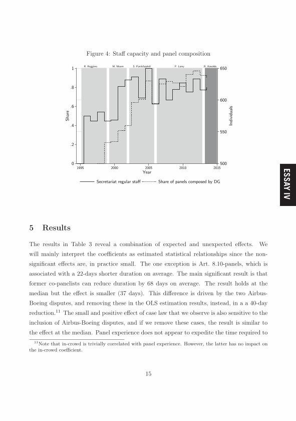
ESSAY IV

Figure 3: Duration and Eq. days per claim, over time.

50

100

150

200

250

Day

s per

clai

m

200

400

600

800

1000

Day

s

1995 2000 2005 2010 2015Year

Average duration Eq. days per claim

Although the number of requests for panel adjudication has been steady in the last

years, Figure 4 shows that the Secretariat’s panel composition duties have increased over

time. If we take Figure 4 as evidence of a general increase in workload, we would expect

that the time to complete panel proceedings would also have increased. But this is not

reflected in Figure 2, suggesting, perhaps, that the increase in staff capacity has somewhat

compensated the increasing demands of the DSM.

14

Figure 4: Staff capacity and panel composition

R. Ruggiero M. Moore S. Panitchpakdi P. Lamy R. Azevêdo

500

550

600

650

Indi

vidua

ls

0

.2

.4

.6

.8

1Sh

are

1995 2000 2005 2010 2015Year

Secretariat regular staff Share of panels composed by DG

5 Results

The results in Table 3 reveal a combination of expected and unexpected effects. We

will mainly interpret the coefficients as estimated statistical relationships since the non-

significant effects are, in practice small. The one exception is Art. 8.10-panels, which is

associated with a 22-days shorter duration on average. The main significant result is that

former co-panelists can reduce duration by 68 days on average. The result holds at the

median but the effect is smaller (37 days). This difference is driven by the two Airbus-

Boeing disputes, and removing these in the OLS estimation results, instead, in a a 40-day

reduction.11 The small and positive effect of case law that we observe is also sensitive to the

inclusion of Airbus-Boeing disputes, and if we remove these cases, the result is similar to

the effect at the median. Panel experience does not appear to expedite the time required to11Note that in-crowd is trivially correlated with panel experience. However, the latter has no impact on

the in-crowd coefficient.

15

issue panel reports, which confirms the findings in Horn (2013) and Busch and Pelc (2009).

As expected, working on multiple panels concurrently increases duration by over 100

days (median). But it is unlikely that this would be the case for a permanent panel that

handles multiple panels. For example, the AB consistently met their 90-day deadline up

until 2014, when they were overwhelmed by a sudden increase in appeals. Appointed ad

hoc panelists are hardly expected to work full-time on a case (Johannesson and Mavroidis,

2015), even if they are assigned multiple ones. Thus, it is difficult to calculate the trade-

off in time between a full-time, and a more efficient, permanent panel and the increased

workload it would entail.

Next, we discuss if experience and in-crowd are positively associated with efficiency.

Unexpectedly, Eq. days per day appears to suffer with panel experience, though not by

much. Each prior panel experience adds around 5 more Eq. days per claim. For 10 claims,

that would amount to 16 extra days, although the effect is diminishing after a combined

panel experience of twelve.12 These effects are most likely explained by selection effects:

As a panelist amasses experience, the chances of being appointed increase, but at the same

time, panelists with experience are more likely to be assigned more complex and therefore

time-consuming cases. The magnitudes are similar at the median, though not significant.

We do not observe any positive effects on efficiency when working with previous co-panelists.

Lastly, panels that were appointed by the DG are associated with both a 40-day increase

in duration and a 20-day increase in Eq. days per claim, but these results are not robust

as they disappear at the median. However, when we remove the Airbus-Boeing disputes

in OLS, the associated increase is instead 27 Eq. days per claim, but it is not statistically

significant. Considering the steady increase in disputes that refer the panel composition to

the DG, as seen in Figure 4, the relationship between DG-appointed panels and complexity

may not be as strong as theorized. It is possible that the parties seek the assistance of the

DG more often simply out of convenience and time considerations, rather than an increase

in politically sensitive disputes.

Before concluding, it is important to keep in mind that we implicitly assumed constant

quality when we interpreted the results. That is, efficiency gains are not achieved at the

expense of quality in rulings. But, clearly, for some minimum value of Eq. days per claim,12 ∂yxd

x

[γ1x+ γ2x

2]= 4.7 + 2 · (−0.20x) = 0 ⇔ x = 12

16

additional time-saving efforts will probably affect the quality of the panel report negatively.

Table 3: OLS regression

Duration Eq. days per claim

No. of claims 2.3* −1.6***(1.0) (0.25)

Expert 250*** 93***(54) (23)

Total Panel Experience 7.9 4.7’(7.5) (2.6)

Total Panel Experience (squared) −0.32 −0.20’(0.26) (0.10)

Domestic instrument disputes 1.3 −3.0(24) (11)

Case law 1.5* 0.13(0.71) (0.25)

Case law || DI cases 0.34 −0.29(1.4) (0.42)

No. of Third Parties 4.0’ −1.4’(2.3) (0.75)

Appointed by DG 42’ 21’(25) (11)

Multiple panels 178* 49*(89) (19)

In-crowd −68* −4.1(31) (10)

In-crowd || DG 14 −5.3(15) (8.9)

Art. 8.10 composition −22 11(22) (10)

(constant) 226*** 126***(22) (10)

R2 0.36 0.41N 210 210

*** p < 0.1%, ** p < 1%, * p < 5%, ’ p < 10%

17

ESSAY IV

issue panel reports, which confirms the findings in Horn (2013) and Busch and Pelc (2009).

As expected, working on multiple panels concurrently increases duration by over 100

days (median). But it is unlikely that this would be the case for a permanent panel that

handles multiple panels. For example, the AB consistently met their 90-day deadline up

until 2014, when they were overwhelmed by a sudden increase in appeals. Appointed ad

hoc panelists are hardly expected to work full-time on a case (Johannesson and Mavroidis,

2015), even if they are assigned multiple ones. Thus, it is difficult to calculate the trade-

off in time between a full-time, and a more efficient, permanent panel and the increased

workload it would entail.

Next, we discuss if experience and in-crowd are positively associated with efficiency.

Unexpectedly, Eq. days per day appears to suffer with panel experience, though not by

much. Each prior panel experience adds around 5 more Eq. days per claim. For 10 claims,

that would amount to 16 extra days, although the effect is diminishing after a combined

panel experience of twelve.12 These effects are most likely explained by selection effects:

As a panelist amasses experience, the chances of being appointed increase, but at the same

time, panelists with experience are more likely to be assigned more complex and therefore

time-consuming cases. The magnitudes are similar at the median, though not significant.

We do not observe any positive effects on efficiency when working with previous co-panelists.

Lastly, panels that were appointed by the DG are associated with both a 40-day increase

in duration and a 20-day increase in Eq. days per claim, but these results are not robust

as they disappear at the median. However, when we remove the Airbus-Boeing disputes

in OLS, the associated increase is instead 27 Eq. days per claim, but it is not statistically

significant. Considering the steady increase in disputes that refer the panel composition to

the DG, as seen in Figure 4, the relationship between DG-appointed panels and complexity

may not be as strong as theorized. It is possible that the parties seek the assistance of the

DG more often simply out of convenience and time considerations, rather than an increase

in politically sensitive disputes.

Before concluding, it is important to keep in mind that we implicitly assumed constant

quality when we interpreted the results. That is, efficiency gains are not achieved at the

expense of quality in rulings. But, clearly, for some minimum value of Eq. days per claim,12 ∂yxd

x

[γ1x+ γ2x

2]= 4.7 + 2 · (−0.20x) = 0 ⇔ x = 12

16

additional time-saving efforts will probably affect the quality of the panel report negatively.

Table 3: OLS regression


No. of claims 2.3* −1.6***(1.0) (0.25)

Expert 250*** 93***(54) (23)

Total Panel Experience 7.9 4.7’(7.5) (2.6)

Total Panel Experience (squared) −0.32 −0.20’(0.26) (0.10)

Domestic instrument disputes 1.3 −3.0(24) (11)

Case law 1.5* 0.13(0.71) (0.25)

Case law || DI cases 0.34 −0.29(1.4) (0.42)

No. of Third Parties 4.0’ −1.4’(2.3) (0.75)

Appointed by DG 42’ 21’(25) (11)

Multiple panels 178* 49*(89) (19)

In-crowd −68* −4.1(31) (10)

In-crowd || DG 14 −5.3(15) (8.9)

Art. 8.10 composition −22 11(22) (10)

(constant) 226*** 126***(22) (10)

R2 0.36 0.41N 210 210

*** p < 0.1%, ** p < 1%, * p < 5%, ’ p < 10%

17

Table 4: Median regression (robustness)


No. of claims 2.0*** −1.4***(0.42) (0.23)

Expert 215*** 77***(35) (20)

Total Panel Experience 5.6 3.7(5.2) (2.9)

Total Panel Experience (squared) −0.27 −0.18(0.28) (0.16)

Domestic instrument disputes 6.0 6.9(23) (13)

Case law 0.51 0.067(0.62) (0.34)

Case law || DI cases 0.91 0.26(1.2) (0.65)

No. of Third Parties 6.7*** −0.57(2.0) (1.1)

Appointed by DG 2.1 5.8(23) (13)

Multiple panels 105** 26(35) (20)

In-crowd −37* 3.4(19) (10)

In-crowd || DG 12 −3.9(16) (9.1)

Art. 8.10 composition 2.7 14(26) (14)

(constant) 221*** 106***(26) (14)

N 210 210

*** p < 0.1%, ** p < 1%, * p < 5%, ’ p < 10%

18

5.1 Robustness

Table 5: Comparison of coefficients

(I) (II) (III)OLS Median OLS Median OLS Median

Duration 7.9 5.6 -68.4 -37.1 1.5 0.5(7.5) (5.2) (31.0) (18.5) (0.7) (0.6)

Eq. days per claim 4.7 3.7 -4.1 3.4 0.1 0.1(2.6) (2.9) (10.2) (10.4) (0.2) (0.3)

Days per claim (equal weight) 3.1 0.5 12.4 10.1 -0.1 -0.1(2.0) (2.1) (11.3) (7.7) (0.2) (0.3)

Days per unique claim (equal weight) 2.5 0.9 11.9 11.4 0.4 0.2(2.8) (3.7) (12.9) (13.4) (0.3) (0.4)

Eq. days per unique claim 3.6 3.3 -8.2 -9.3 0.8 0.4(3.6) (4.0) (14.4) (14.5) (0.3) (0.5)

(I) Panel Experience (II) In-crowd (III) Case Law

We compare three panel-related variables: panel experience, In-crowd and case law

across different variants of duration and efficiency (see Appendix E for full regression tables

and Figure A.3 in Appendix A for variation over time). Then OLS coefficients remain

insignificant for both panel experience and case law for all specifications. In-crowd, however,

is sensitive to the functional form. If we apply equal weights to the claims, the variable

in-crowd is associated with an increase of 12 days per claim, on average.

6 Discussion

The problem of delays in panel deliberations have been a long-standing issue, going as far

back as the GATT (Tuthill et al., 1985). But in recent years, the problem has intensified

with the success of the DSM. One suggestion on how to improve the system has been to

replace ad hoc panels with permanent ones. This study offers some new insights on the

association between time, efficiency and panel features that characterize permanent panels.

Apart from using the time it takes for panels to issue panel reports to measure timeliness,

we also measure efficiency, using Eq. days per claim, which is constructed by taking the

19

ESSAY IV

Table 4: Median regression (robustness)


No. of claims 2.0*** −1.4***(0.42) (0.23)

Expert 215*** 77***(35) (20)

Total Panel Experience 5.6 3.7(5.2) (2.9)

Total Panel Experience (squared) −0.27 −0.18(0.28) (0.16)

Domestic instrument disputes 6.0 6.9(23) (13)

Case law 0.51 0.067(0.62) (0.34)

Case law || DI cases 0.91 0.26(1.2) (0.65)

No. of Third Parties 6.7*** −0.57(2.0) (1.1)

Appointed by DG 2.1 5.8(23) (13)

Multiple panels 105** 26(35) (20)

In-crowd −37* 3.4(19) (10)

In-crowd || DG 12 −3.9(16) (9.1)

Art. 8.10 composition 2.7 14(26) (14)

(constant) 221*** 106***(26) (14)

N 210 210

*** p < 0.1%, ** p < 1%, * p < 5%, ’ p < 10%

18

5.1 Robustness

Table 5: Comparison of coefficients

(I) (II) (III)OLS Median OLS Median OLS Median

Duration 7.9 5.6 -68.4 -37.1 1.5 0.5(7.5) (5.2) (31.0) (18.5) (0.7) (0.6)

Eq. days per claim 4.7 3.7 -4.1 3.4 0.1 0.1(2.6) (2.9) (10.2) (10.4) (0.2) (0.3)

Days per claim (equal weight) 3.1 0.5 12.4 10.1 -0.1 -0.1(2.0) (2.1) (11.3) (7.7) (0.2) (0.3)

Days per unique claim (equal weight) 2.5 0.9 11.9 11.4 0.4 0.2(2.8) (3.7) (12.9) (13.4) (0.3) (0.4)

Eq. days per unique claim 3.6 3.3 -8.2 -9.3 0.8 0.4(3.6) (4.0) (14.4) (14.5) (0.3) (0.5)

(I) Panel Experience (II) In-crowd (III) Case Law

We compare three panel-related variables: panel experience, In-crowd and case law

across different variants of duration and efficiency (see Appendix E for full regression tables

and Figure A.3 in Appendix A for variation over time). Then OLS coefficients remain

insignificant for both panel experience and case law for all specifications. In-crowd, however,

is sensitive to the functional form. If we apply equal weights to the claims, the variable

in-crowd is associated with an increase of 12 days per claim, on average.

6 Discussion

The problem of delays in panel deliberations have been a long-standing issue, going as far

back as the GATT (Tuthill et al., 1985). But in recent years, the problem has intensified

with the success of the DSM. One suggestion on how to improve the system has been to

replace ad hoc panels with permanent ones. This study offers some new insights on the

association between time, efficiency and panel features that characterize permanent panels.

Apart from using the time it takes for panels to issue panel reports to measure timeliness,

we also measure efficiency, using Eq. days per claim, which is constructed by taking the

19

duration and divide it by the square root of number of claims. In this manner, we are able

to account for economies of scale in examining claims.

We will focus our discussion on three main results. First, one of the main arguments

for permanent panels is that experience matters for both the quality of panel reports and

efficiency of panel work (Busch and Pelc, 2009), and permanent panels will ensure that

judges accumulate such experience. Our results show, however, that panel experience does

not have any substantial impact on duration. Although we found positive effects on Eq.

days per claim—most likely due to selection effects—the effect is small, making it difficult

to infer anything credible about its role in time-saving.

Second, as found previously in Horn (2013), case law has trivial effects on timeliness

and efficiency. This is a rather counter-intuitive result. One explanation may be that there

is no rule of either vertical or horizontal stare decisis in the DSM. That is, neither previous

panel rulings nor the rulings of the Appellate Body are binding, although the panel is

permitted to consult them. Hence, a large body of case law is not as helpful as one might

think. There has been a long-standing belief that a de facto stare decisis has developed in

the DSM, particularly since the AB has insisted that the panel (and the AB itself) follow

AB jurisprudence (see DS 344, DS 322). Although there have been relatively few instances

of explicit tension between the panel and AB rulings, aside from the mentioned disputes,

the token effect of case law on timeliness may suggest that panels do not, in general, apply

stare decisis. If this is the case, a panelist’s experience should be even more important as

case law could have been a way to support less experienced panelists.

Third, panels that consist of former co-panelists were associated with the largest re-

duction in duration. Two panelists that have worked together previously is associated with

a 40-day decrease in the time it takes to issue panel reports. We do not have a causal frame-

work, so there could be several explanations for this result apart from the straightforward

one, that an established work relationship can expedite panel deliberations. We previously

discussed that the lack of results from panel experience could be due to selection effects,

and the same could be true for in-crowd; former co-panelists are more likely to be appoin-

ted specific disputes that, for various reasons, take a shorter amount of time to complete.

However, it is difficult to surmise what type of dispute characteristics would cause such a

mechanism.

20

References

Bourgeois, J. H. (2003). Comment on a WTO permanent panel body. Journal of Interna-

tional Economic Law 6 (1), 211.

Busch, M. L. and K. J. Pelc (2009). Does the WTO need a permanent body of panelists?

Journal of International Economic Law 12 (3), 579.

Cottier, T. (2003). The WTO permanent panel body: a bridge too far? Journal of

International Economic Law 6 (1), 187.

Davey, W. J. (2003). The case for a WTO permanent panel body. Journal of International

Economic Law 6 (1), 177.

Horn, H. (2013). The time WTO panels require to issue reports. Working paper no. 979,

Research Institute of Industrial Economics.

Horn, H., G. Maggi, and R. W. Staiger (2010). Trade agreements as endogenously incom-

plete contracts. The American Economic Review 100 (1), 394–419.

Howse, R. (2012). Regulatory Measures. In A. Narlikar, M. Daunton, and R. M. Stern

(Eds.), The Oxford Handbook on the World Trade Organization. Oxford University Press.

Hudec, R. E. (1999). The new WTO dispute settlement procedure: an overview of the first

three years. Minn. J. Global Trade 8, 1.

Jackson, J. H. (1979). Governmental disputes in international trade relations: a proposal

in the context of gatt. J. World Trade L. 13, 1.

Johannesson, L. and P. C. Mavroidis (2015). Black Cat , White Cat : The Identity of the

WTO Judges. Journal of World Trade 49 (4), 685–698.

Tuthill, L. L., J. E. Guth, K. A. Skidmore, and P. Gibson (1985). Review of the effectiveness

of trade dispute settlement under the Gatt and the Tokyo Round agreements : report to the

Committee on Finance, U.S. Senate, on investigation no. 332-212 under section 332(g)

of the Tariff Act of 1930. Number 1793 in USITC publication. Washington, DC : U.S.

International Trade Commission.

21

ESSAY IV

duration and divide it by the square root of number of claims. In this manner, we are able

to account for economies of scale in examining claims.

We will focus our discussion on three main results. First, one of the main arguments

for permanent panels is that experience matters for both the quality of panel reports and

efficiency of panel work (Busch and Pelc, 2009), and permanent panels will ensure that

judges accumulate such experience. Our results show, however, that panel experience does

not have any substantial impact on duration. Although we found positive effects on Eq.

days per claim—most likely due to selection effects—the effect is small, making it difficult

to infer anything credible about its role in time-saving.

Second, as found previously in Horn (2013), case law has trivial effects on timeliness

and efficiency. This is a rather counter-intuitive result. One explanation may be that there

is no rule of either vertical or horizontal stare decisis in the DSM. That is, neither previous

panel rulings nor the rulings of the Appellate Body are binding, although the panel is

permitted to consult them. Hence, a large body of case law is not as helpful as one might

think. There has been a long-standing belief that a de facto stare decisis has developed in

the DSM, particularly since the AB has insisted that the panel (and the AB itself) follow

AB jurisprudence (see DS 344, DS 322). Although there have been relatively few instances

of explicit tension between the panel and AB rulings, aside from the mentioned disputes,

the token effect of case law on timeliness may suggest that panels do not, in general, apply

stare decisis. If this is the case, a panelist’s experience should be even more important as

case law could have been a way to support less experienced panelists.

Third, panels that consist of former co-panelists were associated with the largest re-

duction in duration. Two panelists that have worked together previously is associated with

a 40-day decrease in the time it takes to issue panel reports. We do not have a causal frame-

work, so there could be several explanations for this result apart from the straightforward

one, that an established work relationship can expedite panel deliberations. We previously

discussed that the lack of results from panel experience could be due to selection effects,

and the same could be true for in-crowd; former co-panelists are more likely to be appoin-

ted specific disputes that, for various reasons, take a shorter amount of time to complete.

However, it is difficult to surmise what type of dispute characteristics would cause such a

mechanism.

20

References

Bourgeois, J. H. (2003). Comment on a WTO permanent panel body. Journal of Interna-

tional Economic Law 6 (1), 211.

Busch, M. L. and K. J. Pelc (2009). Does the WTO need a permanent body of panelists?

Journal of International Economic Law 12 (3), 579.

Cottier, T. (2003). The WTO permanent panel body: a bridge too far? Journal of

International Economic Law 6 (1), 187.

Davey, W. J. (2003). The case for a WTO permanent panel body. Journal of International

Economic Law 6 (1), 177.

Horn, H. (2013). The time WTO panels require to issue reports. Working paper no. 979,

Research Institute of Industrial Economics.

Horn, H., G. Maggi, and R. W. Staiger (2010). Trade agreements as endogenously incom-

plete contracts. The American Economic Review 100 (1), 394–419.

Howse, R. (2012). Regulatory Measures. In A. Narlikar, M. Daunton, and R. M. Stern

(Eds.), The Oxford Handbook on the World Trade Organization. Oxford University Press.

Hudec, R. E. (1999). The new WTO dispute settlement procedure: an overview of the first

three years. Minn. J. Global Trade 8, 1.

Jackson, J. H. (1979). Governmental disputes in international trade relations: a proposal

in the context of gatt. J. World Trade L. 13, 1.

Johannesson, L. and P. C. Mavroidis (2015). Black Cat , White Cat : The Identity of the

WTO Judges. Journal of World Trade 49 (4), 685–698.

Tuthill, L. L., J. E. Guth, K. A. Skidmore, and P. Gibson (1985). Review of the effectiveness

of trade dispute settlement under the Gatt and the Tokyo Round agreements : report to the

Committee on Finance, U.S. Senate, on investigation no. 332-212 under section 332(g)

of the Tariff Act of 1930. Number 1793 in USITC publication. Washington, DC : U.S.

International Trade Commission.

21

A Data

Figure A.1: Square root equivalence scale

0

200

400

600

Day

s

0 50 100 150No. of claims

A.1 Variables

Figure A.4 plots the distribution of some of the variables that we include in the analysis.

Note that the values are plotted against each dispute’s DS number, which can be interpreted

as time since these numbers are cumulative.

22

Figure A.2: Duration

Figure A.3: Alternative outcomes

20

40

60

80

100

120

Day

s (al

l cla

ims)

0

100

200

300

400

Day

s (un

ique

clai

ms)

1995 2000 2005 2010 2015Year

Eq. days per unique claim Days per unique claimDays per claim

23

ESSAY IV

A Data

Figure A.1: Square root equivalence scale

0

200

400

600

Day

s

0 50 100 150No. of claims

A.1 Variables

Figure A.4 plots the distribution of some of the variables that we include in the analysis.

Note that the values are plotted against each dispute’s DS number, which can be interpreted

as time since these numbers are cumulative.

22

Figure A.2: Duration

Figure A.3: Alternative outcomes

20

40

60

80

100

120

Day

s (al

l cla

ims)

0

100

200

300

400

Day

s (un

ique

clai

ms)

1995 2000 2005 2010 2015Year

Eq. days per unique claim Days per unique claimDays per claim

23

Figure A.4: Variables

(a) Total number of claims (b) Panel Experience

(c) Third parties (d) Case Law

24

B Participation

Figure A.5: Request for consultations, complainants to respondentsratio

0

2

4

6

Com

plain

ants

to R

espo

nden

ts ra

tio

1995 2000 2005 2010 2015Year

US/EU Rest of the Membership

C Director-Generals

Table A.1 presents all WTO DGs and their respective terms (four years). The current DG,

Roberto Azevêdo, was appointed in late 2013.13

Table A.1: Director-Generals

Director-General Years Nationality #Panels #Panels by DGRenato Ruggiero 1995--1999 Italy 70 29Mike Moore 2000--2002 New Zealand 48 36Supachai Panitchpakdi 2003--2005 Thailand 33 27Pascal Lamy 2006--2013 France 77 57Roberto Azevêdo 2014-- Brazil 5 4

13The procedural guidelines to appoint a DG was adopted in 2002 and is described in WT/L/509.

25

ESSAY IV

Figure A.4: Variables

(a) Total number of claims (b) Panel Experience

(c) Third parties (d) Case Law

24

B Participation

Figure A.5: Request for consultations, complainants to respondentsratio

0

2

4

6

Com

plain

ants

to R

espo

nden

ts ra

tio

1995 2000 2005 2010 2015Year

US/EU Rest of the Membership

C Director-Generals

Table A.1 presents all WTO DGs and their respective terms (four years). The current DG,

Roberto Azevêdo, was appointed in late 2013.13

Table A.1: Director-Generals

Director-General Years Nationality #Panels #Panels by DGRenato Ruggiero 1995--1999 Italy 70 29Mike Moore 2000--2002 New Zealand 48 36Supachai Panitchpakdi 2003--2005 Thailand 33 27Pascal Lamy 2006--2013 France 77 57Roberto Azevêdo 2014-- Brazil 5 4

13The procedural guidelines to appoint a DG was adopted in 2002 and is described in WT/L/509.

25

D Country classification

Table A.2: Country Classification

IND DEVAustralia Antigua and BarbudaCanada ArgentinaJapan ChileKorea Chinese TaipeiMexico ColombiaNew Zealand Costa RicaNorway Dominican RepublicPoland EcuadorSwitzerland EgyptTurkey El Salvador

GuatemalaG2 HondurasEU IndonesiaUS Malaysia

PakistanBRIC PanamaBrazil PeruChina PhilippinesIndia Thailand

UkraineVenezuelaViet Nam

E Alternative specifications

The outcomes in Table A.3 and A.4 are defined as follows: (1) days per claim, equal weights;

(2) days per unique claim, equal weights and; (3) Eq. days per unique claim.

26

Table A.3: Alternative outcomes: OLS regression

(1) (2) (3)

No. of claims −1.3*** −1.1*** −0.83*(0.21) (0.24) (0.36)

Expert 39** 48** 111***(13) (18) (24)

Total Panel Experience 3.1 2.5 3.6(2.0) (2.8) (3.6)

Total Panel Experience (squared) −0.13 −0.19 −0.24(0.093) (0.13) (0.15)

Domestic instrument disputes −6.3 −8.4 −7.9(9.8) (12) (13)

Case law −0.14 0.43 0.80*(0.19) (0.26) (0.35)

Case law || DI cases −0.26 0.12 −0.026(0.34) (0.64) (0.68)

No. of Third Parties −2.1** −2.8** −1.3(0.73) (1.0) (1.1)

Appointed by DG 10 22’ 28*(11) (12) (13)

Multiple panels 19 42* 72*(14) (21) (34)

In-crowd 12 12 −8.2(11) (13) (14)

In-crowd || DG −14 −13 −0.98(11) (12) (10)

Art. 8.10 composition 18’ 15 −0.11(11) (17) (14)

(constant) 72*** 85*** 133***(11) (13) (12)

R2 0.35 0.25 0.23N 210 210 210

*** p < 0.1%, ** p < 1%, * p < 5%, ’ p < 10%

27

ESSAY IV

D Country classification

Table A.2: Country Classification

IND DEVAustralia Antigua and BarbudaCanada ArgentinaJapan ChileKorea Chinese TaipeiMexico ColombiaNew Zealand Costa RicaNorway Dominican RepublicPoland EcuadorSwitzerland EgyptTurkey El Salvador

GuatemalaG2 HondurasEU IndonesiaUS Malaysia

PakistanBRIC PanamaBrazil PeruChina PhilippinesIndia Thailand

UkraineVenezuelaViet Nam

E Alternative specifications

The outcomes in Table A.3 and A.4 are defined as follows: (1) days per claim, equal weights;

(2) days per unique claim, equal weights and; (3) Eq. days per unique claim.

26

Table A.3: Alternative outcomes: OLS regression

(1) (2) (3)

No. of claims −1.3*** −1.1*** −0.83*(0.21) (0.24) (0.36)

Expert 39** 48** 111***(13) (18) (24)



Domestic instrument disputes −6.3 −8.4 −7.9(9.8) (12) (13)

Case law −0.14 0.43 0.80*(0.19) (0.26) (0.35)

Case law || DI cases −0.26 0.12 −0.026(0.34) (0.64) (0.68)

No. of Third Parties −2.1** −2.8** −1.3(0.73) (1.0) (1.1)

Appointed by DG 10 22’ 28*(11) (12) (13)

Multiple panels 19 42* 72*(14) (21) (34)

In-crowd 12 12 −8.2(11) (13) (14)

In-crowd || DG −14 −13 −0.98(11) (12) (10)

Art. 8.10 composition 18’ 15 −0.11(11) (17) (14)

(constant) 72*** 85*** 133***(11) (13) (12)

R2 0.35 0.25 0.23N 210 210 210

*** p < 0.1%, ** p < 1%, * p < 5%, ’ p < 10%

27

Table A.4: Alternative outcomes: median regression

(1) (2) (3)

No. of claims −0.81*** −0.74* −0.81*(0.17) (0.30) (0.33)

Expert 32* 68** 152***(15) (25) (27)



Domestic instrument disputes 4.4 −4.4 −12(9.4) (16) (18)

Case law −0.13 0.19 0.44(0.26) (0.44) (0.48)

Case law || DI cases −0.20 −0.20 0.60(0.49) (0.84) (0.92)

No. of Third Parties −1.2 −0.40 −0.63(0.83) (1.4) (1.6)

Appointed by DG 5.9 6.2 −1.2(9.7) (17) (18)

Multiple panels 3.2 −2.5 37(15) (25) (27)

In-crowd 10 11 −9.3(7.7) (13) (15)

In-crowd || DG −8.0 −2.9 14(6.8) (12) (13)

Art. 8.10 composition 8.1 −1.8 −6.8(11) (18) (20)

(constant) 47*** 54** 128***(11) (19) (20)

N 210 210 210

*** p < 0.1%, ** p < 1%, * p < 5%, ’ p < 10%

28

ESSAY V

Are WTO disputes public goods?—Dispute effects for the

membership


1 Introduction

The dispute settlement mechanism (DSM) in the World Trade Organization (WTO) is one ofthe most active forums for international dispute resolution, yet only a handful of the members, 35%,have actively participated so far. Furthermore, over 70% of the cases involve either the US or theEU, or both. This aspect of the DSM has raised concern that some members—most notably thepoorer countries—are unable to access the system because of various systemic reasons. One suchreason that is often cited as an obstacle to active participation is the high cost of litigation (Bownand Hoekman, 2005; Bohanes and Garza, 2012). When the WTO was established, in 1995, toreplace the provisional trade agreement GATT, the DSM underwent a significant structural reform,which brought about a stricter judicial process for settling disputes. This led to improvements intransparency and reliability, which expedited the litigation process, but at the same time, adju-dication became more legally complex, making the process more expensive. This observation byKim (2008) may explain, in part, why there have not been any substantial changes in the share ofactive countries since the GATT, which was then around 30%. Thus, participation rate, and theselection of complainants, in the DSM is likely a result of both institutional design and countrycharacteristics. On the other hand, selective participation is to be expected since a higher varietyof exports and number of trade relations will increase the probability of encountering actionabletrade policies (Horn et al., 2005; Sattler and Bernauer, 2011; Busch and Reinhardt, 2003). Thus,it is difficult to know how much a policy intervention could broaden participation.

∗Research Institute of Industrial Economics, Box 55665, SE-102 15 Stockholm and Örebro University, Sweden.E-mail: [email protected]. For valuable comments, I would like to express my gratitude to Henrik Horn atIFN, Magnus Lodefalk and Dan Johansson at Örebro University, and Hildegunn Kyvik Nordås at the OECD. I wouldalso like to thank the seminar participants at IFN and Maria Persson at Lund University. I gratefully acknowledgesfinancial support from the Jan Wallander and Tom Hedelius Foundation and the Marianne and Marcus WallenbergFoundation.

1

ESSAY V

Are WTO disputes public goods?—Dispute effects for the

membership


1 Introduction

The dispute settlement mechanism (DSM) in the World Trade Organization (WTO) is one ofthe most active forums for international dispute resolution, yet only a handful of the members, 35%,have actively participated so far. Furthermore, over 70% of the cases involve either the US or theEU, or both. This aspect of the DSM has raised concern that some members—most notably thepoorer countries—are unable to access the system because of various systemic reasons. One suchreason that is often cited as an obstacle to active participation is the high cost of litigation (Bownand Hoekman, 2005; Bohanes and Garza, 2012). When the WTO was established, in 1995, toreplace the provisional trade agreement GATT, the DSM underwent a significant structural reform,which brought about a stricter judicial process for settling disputes. This led to improvements intransparency and reliability, which expedited the litigation process, but at the same time, adju-dication became more legally complex, making the process more expensive. This observation byKim (2008) may explain, in part, why there have not been any substantial changes in the share ofactive countries since the GATT, which was then around 30%. Thus, participation rate, and theselection of complainants, in the DSM is likely a result of both institutional design and countrycharacteristics. On the other hand, selective participation is to be expected since a higher varietyof exports and number of trade relations will increase the probability of encountering actionabletrade policies (Horn et al., 2005; Sattler and Bernauer, 2011; Busch and Reinhardt, 2003). Thus,it is difficult to know how much a policy intervention could broaden participation.

∗Research Institute of Industrial Economics, Box 55665, SE-102 15 Stockholm and Örebro University, Sweden.E-mail: [email protected]. For valuable comments, I would like to express my gratitude to Henrik Horn atIFN, Magnus Lodefalk and Dan Johansson at Örebro University, and Hildegunn Kyvik Nordås at the OECD. I wouldalso like to thank the seminar participants at IFN and Maria Persson at Lund University. I gratefully acknowledgesfinancial support from the Jan Wallander and Tom Hedelius Foundation and the Marianne and Marcus WallenbergFoundation.

1

It is indeed a complex task to uncover the many different determinants and mechanisms thatinfluence dispute initiation. However, a fairly simple formulation of this decision is that countrieswill decide to participate if their expected benefit of prevailing at the DSM is greater than theexpected cost (Bown, 2005). Although this implies that disputes will not necessarily be selectedbecause the expected benefit is limited to the complainant, but because they have the highest benefitrelative to cost among the members. In Bown and Reynolds (2015), it is shown that complainants’exports are indeed much larger than non-complainants and that they experience a larger drop inexports when a respondent restricts market access. Since the WTO is founded on the principleof non-discrimination, other members are aware that any ruling, or bilateral settlement for thatmatter, in favour of the complainant must be extended to the membership (Bown, 2005). Thus,there is little incentive for members with a stake in the case to join the complainant and share thelitigation costs once a complaint has been filed. However, this hypothesis is dependent on therebeing no differential dispute effects between complainants and non-complainants.

A few studies have examined differential gains from disputes between complainants and non-complainants, such as Kucik and Pelc (2016). They examined differences in respondent-specificimports between complainants and the membership but found no such differences for disputes thatwere formally adjudicated. But they did find evidence of discriminatory outcomes for disputesthat settled early. Part of the explanation could be different types of trade policies. In Bown andReynolds (2015), two types of of trade policies are distinguished: global policies that affect allexporters, and partial policies that mainly affect the complainants. They show that there is a signi-ficant difference in import changes on the respondents’ markets between partial and global policies.Furthermore, complainants experience larger reductions in exports compared to the membership.Bechtel and Sattler (2015) investigated potential differences in dispute effects between complainantsand third parties—their analysis excluded the rest of the membership however. They estimated thecausal effect of a panel ruling on respondent’s sector-level import flows using a matching approach,but found no differential effects.

Although there seems to be convincing arguments for relative dispute effects between the com-plainants and non-complainants, relative effects are, however, only detectable if the disputed trademeasure, or the subsequent resolution, discriminated between complainants and non-complainants.In any other case, relative effects will not be measurable even if the dispute led to positive tradeeffects for the whole membership. Thus, to understand the broader impact of WTO disputes it isimportant to also understand the absolute effect of a dispute for all members. Something that was,in part, studied by Chaudoin et al. (2016) who examined dispute effects on respondents’ importsby comparing it to other import markets. They did not, however, find any positive effects, butbecause they used an importer-year panel structure rather than bilateral trade flows, as done inthe previous studies, they were unable to explore any exporter-specific effects. The evidence sofar, seems to indicate that there are dispute effects between exporters, i.e. complainants and non-

2

complainants, on the respondent’s market but no general effects between importers, i.e. respondentsand non-respondents.

In this paper, we seek to estimate potential dispute effects for seemingly affected membersthat are not actively participating in the dispute. We do this by examining trade flow changes ofdisputed products before and after a dispute using bilateral trade flows at the 4-digit product levelof the Harmonized System (HS) codes. Thus, we are able to distinguish between the exporters,enabling us to separate non-complainants from complainants and co-complainants, and also toidentify respondents and non-respondents among the importers. In order to credibly measurethe absolute dispute effect of disputes, we apply a Difference-in-Differences framework where wecompare exporter-specific trade flows between respondents and non-respondents. Since disputesare filed at different years, we estimate a model with staggered treatment where, for each dispute,time is normalized to the year of dispute initiation. As a benchmark, we use two alternative controlmarkets. For the first control group alternative, we define comparable markets (to the respondents)by first identifying all exporters that trade in the disputed products to the respondents’ markets,and in a second step, identify all other export destinations, that are not the respondents, for theseexporters; we will denote these as the primary control markets. This has also a flip side, becausean exporter was possibly affected by both the dispute and the trade measure on the respondent’smarket, which ostensibly prompted the complaint. It is therefore possible that this had rippleeffects to the exporter’s other trading relations for the same products. If this is the case, a crucialassumption of the Difference-in-Differences framework would be violated: the control group musthave been unaffected by the dispute (i.e. no spillover effects). For this reason, we introduce asecond control group: import markets that were excluded in the definition of the primary controlmarkets because they were not export destinations for the affected exporters in question; thatis, these markets trade with exporters that were not directly affected by the trade measure andthe subsequent dispute. We use this group of “independent” import markets as secondary controlmarkets to validate our results from using the primary control markets. Furthermore, given theassumption of zero spillover effects on the secondary control markets, we also use these controlsto quantify possible spillover effects on the primary control markets, something which is ordinarilydifficult to measure in a DD setting. To achieve as comparable markets as possible, we dividethe products further into agricultural and manufacturing goods as the former is characterizedby imperfect competition issues, such as domestic support and volatile market prices. Becauseagriculture is related to domestic food security issues, this area is also highly contentious in theWTO. Going by the previous literature, we also separate disputes that were formally adjudicatedby a panel from those that were not, where the latter include outcomes such as mutually agreedsolutions (MAS), and abandoned disputes. This may account for some of the underlying disputecharacteristics that may influence both the selection of disputes that escalate to adjudication andtrade outcomes.

3

ESSAY V

It is indeed a complex task to uncover the many different determinants and mechanisms thatinfluence dispute initiation. However, a fairly simple formulation of this decision is that countrieswill decide to participate if their expected benefit of prevailing at the DSM is greater than theexpected cost (Bown, 2005). Although this implies that disputes will not necessarily be selectedbecause the expected benefit is limited to the complainant, but because they have the highest benefitrelative to cost among the members. In Bown and Reynolds (2015), it is shown that complainants’exports are indeed much larger than non-complainants and that they experience a larger drop inexports when a respondent restricts market access. Since the WTO is founded on the principleof non-discrimination, other members are aware that any ruling, or bilateral settlement for thatmatter, in favour of the complainant must be extended to the membership (Bown, 2005). Thus,there is little incentive for members with a stake in the case to join the complainant and share thelitigation costs once a complaint has been filed. However, this hypothesis is dependent on therebeing no differential dispute effects between complainants and non-complainants.

A few studies have examined differential gains from disputes between complainants and non-complainants, such as Kucik and Pelc (2016). They examined differences in respondent-specificimports between complainants and the membership but found no such differences for disputes thatwere formally adjudicated. But they did find evidence of discriminatory outcomes for disputesthat settled early. Part of the explanation could be different types of trade policies. In Bown andReynolds (2015), two types of of trade policies are distinguished: global policies that affect allexporters, and partial policies that mainly affect the complainants. They show that there is a signi-ficant difference in import changes on the respondents’ markets between partial and global policies.Furthermore, complainants experience larger reductions in exports compared to the membership.Bechtel and Sattler (2015) investigated potential differences in dispute effects between complainantsand third parties—their analysis excluded the rest of the membership however. They estimated thecausal effect of a panel ruling on respondent’s sector-level import flows using a matching approach,but found no differential effects.

Although there seems to be convincing arguments for relative dispute effects between the com-plainants and non-complainants, relative effects are, however, only detectable if the disputed trademeasure, or the subsequent resolution, discriminated between complainants and non-complainants.In any other case, relative effects will not be measurable even if the dispute led to positive tradeeffects for the whole membership. Thus, to understand the broader impact of WTO disputes it isimportant to also understand the absolute effect of a dispute for all members. Something that was,in part, studied by Chaudoin et al. (2016) who examined dispute effects on respondents’ importsby comparing it to other import markets. They did not, however, find any positive effects, butbecause they used an importer-year panel structure rather than bilateral trade flows, as done inthe previous studies, they were unable to explore any exporter-specific effects. The evidence sofar, seems to indicate that there are dispute effects between exporters, i.e. complainants and non-

2

complainants, on the respondent’s market but no general effects between importers, i.e. respondentsand non-respondents.

In this paper, we seek to estimate potential dispute effects for seemingly affected membersthat are not actively participating in the dispute. We do this by examining trade flow changes ofdisputed products before and after a dispute using bilateral trade flows at the 4-digit product levelof the Harmonized System (HS) codes. Thus, we are able to distinguish between the exporters,enabling us to separate non-complainants from complainants and co-complainants, and also toidentify respondents and non-respondents among the importers. In order to credibly measurethe absolute dispute effect of disputes, we apply a Difference-in-Differences framework where wecompare exporter-specific trade flows between respondents and non-respondents. Since disputesare filed at different years, we estimate a model with staggered treatment where, for each dispute,time is normalized to the year of dispute initiation. As a benchmark, we use two alternative controlmarkets. For the first control group alternative, we define comparable markets (to the respondents)by first identifying all exporters that trade in the disputed products to the respondents’ markets,and in a second step, identify all other export destinations, that are not the respondents, for theseexporters; we will denote these as the primary control markets. This has also a flip side, becausean exporter was possibly affected by both the dispute and the trade measure on the respondent’smarket, which ostensibly prompted the complaint. It is therefore possible that this had rippleeffects to the exporter’s other trading relations for the same products. If this is the case, a crucialassumption of the Difference-in-Differences framework would be violated: the control group musthave been unaffected by the dispute (i.e. no spillover effects). For this reason, we introduce asecond control group: import markets that were excluded in the definition of the primary controlmarkets because they were not export destinations for the affected exporters in question; thatis, these markets trade with exporters that were not directly affected by the trade measure andthe subsequent dispute. We use this group of “independent” import markets as secondary controlmarkets to validate our results from using the primary control markets. Furthermore, given theassumption of zero spillover effects on the secondary control markets, we also use these controlsto quantify possible spillover effects on the primary control markets, something which is ordinarilydifficult to measure in a DD setting. To achieve as comparable markets as possible, we dividethe products further into agricultural and manufacturing goods as the former is characterizedby imperfect competition issues, such as domestic support and volatile market prices. Becauseagriculture is related to domestic food security issues, this area is also highly contentious in theWTO. Going by the previous literature, we also separate disputes that were formally adjudicatedby a panel from those that were not, where the latter include outcomes such as mutually agreedsolutions (MAS), and abandoned disputes. This may account for some of the underlying disputecharacteristics that may influence both the selection of disputes that escalate to adjudication andtrade outcomes.

3

Our results point to three key findings: first we found positive and significant increases innon-complainants trade flows after a dispute on all import markets. Non-complainants increasedtheir exports by 23% on average to the respondents, or 13 percentage points higher exports tothe respondents compared to primary control markets. Second, if we divide the disputes betweenthose that were adjudicated and those that were not, and we observe that the positive disputeeffect stem mainly from non-adjudicated disputes. In those disputes, the non-active membershipincreased their exports to the respondents by 32%, or 20 percentage points higher dispute effect forrespondents compared to primary control markets. Third, we did not find any dispute effects fornon-complainants in adjudicated disputes. This result, however, does not necessarily imply thatthere are no positive effects for the membership, only that these do not seem to materialize duringthe five-years period that we investigate. This may not be entirely surprising since adjudicateddisputes will naturally take longer to resolve and adjudication itself is generally a sign that theissues are either legally complex or difficult to resolve bilaterally due to political or economicinterests. Taken together, these results seem to imply that non-complainant exporters increasedtheir total exports on all markets after a dispute, but the exports to the respondent was higher indisputes that were settled early.

The paper is organized as follows. The next section describes the the institutional backgroundand the dispute settlement process in a nutshell, and continues with a discussion on the natureof dispute resolutions. Section 3 describes our empirical strategy where we also discuss the issuesof spillover, weighting and Ashenfelter dip. Section 4 describes the data and the limitations thatapply, especially regarding zero and missing trade values. Section 5 presents the results and Section6 concludes with a discussion.

2 When dispute resolution fails

In this section, we will discuss four reasons why we may fail to measure any external trade effectsfor non-active members: first, the dispute lacks legal merit; second, the resolution is discriminatory;third, the disputed trade policy is discriminatory and fourth, the respondent refuse to comply.

The simplest reason for there to be no measurable trade flow changes after a dispute is that thecomplainant was pursuing a weak case. However, it is quite well-established that the success ratein panel is high for complainants (Hoekman et al., 2009; Colares, 2009; Maggi and Staiger, 2011),and in our own data we find that complainants have won around 70% of all claims examined by apanel. The legal merits, and consequently the outcome, for disputes that end before adjudicationare, on the other hand, less transparent since bilateral negotiations are not open to the public.Even though it is mandated by the WTO to issue a notification in case of a settlement, only around36% of these non-adjudicated disputes have done so. The remaining 64% ostensibly languish in

4

prolonged consultations, some as far back as 1995. Though, Alschner (2014) points out that apublic notification is not evidence that a bilateral settlement exists and, conversely, a lack of such isnot necessarily proof that the parties failed to reach an amicable settlement. Indeed, in an extensiveexamination of abandoned cases, Reynolds (2009) found that, as many as 43% had been resolvedin one way or another, some were even resolved in other forums.

Several studies have also argued that privately settled disputes are associated with higher levelof concessions. Such as Busch and Reinhardt (2003) that found that early settlements in disputesbetween the EU and the US, resulted in significantly higher level of concessions compared to disputesthat escalated to panel, with many more full concessions by the respondent in the absence of a panelruling. Yet, these studies also seem to suggest that the benefits of such disputes are limited to thecomplainant. Although privacy, as in closed-door negotiations, is a crucial aspect in reachingbilateral settlements, especially for democracies that are more accountable to domestic interests(Busch and Reinhardt, 2000), Alschner (2014) points out, there is an inherent tension betweenreaching solutions that are bilaterally satisfactory and solutions that fully takes into account therights of the rest of the membership. As previously mentioned, Kucik and Pelc (2016) showed thatprivately settled disputes could lead to discriminatory outcomes, and Guzman and Simmons (2002)argues that the possibility of (bilateral) transfer payments may prevent a case from escalating toadjudication.

A general reason why any resolution could lead to differential effects between the complainantand non-complainants is because the disputed policy itself was discriminatory, such as anti-dumpingduties against certain countries, as discussed in Bown and Reynolds (2015). They found as manyas 60% to be partial policies and the rest, 40%, to be global policies. Contrary to the initialhypothesis that participation is determined by the country with the highest benefit relative to cost,the analysis in Bown and Reynolds (2015) instead suggests that many disputes are selected bythe narrow interests of the complainant. It is therefore likely that any external dispute effect thatwe estimate for the non-participating membership are a result of these global policies. However,a complicating factor is that, even partial policies might have dynamic effects on the extensivemargin. That is, if disputes force a trade-liberalizing policy change, countries that were not presentat the time of the policy implementation might start exporting to the respondent. Thus, even apartial policy might lead to global changes.

Clearly, the merits of a case matters little if the respondent refuses to comply with an adverseruling. An especially relevant consideration in disputes that involve a less powerful complainants,which often lack a credible threat of retaliation (see for example Busch et al., 2009; Bown, 2005).Enforcement in international organizations such as the WTO will, however, always constitute aweakness, as a matter of course. On the other hand, non-compliance may not be as common asone might guess if relatively poorer countries simply refrain from filing a complaint against a richercountry. This is consistent with Wilson (2007) that show that, although complainants are usually

5

ESSAY V

Our results point to three key findings: first we found positive and significant increases innon-complainants trade flows after a dispute on all import markets. Non-complainants increasedtheir exports by 23% on average to the respondents, or 13 percentage points higher exports tothe respondents compared to primary control markets. Second, if we divide the disputes betweenthose that were adjudicated and those that were not, and we observe that the positive disputeeffect stem mainly from non-adjudicated disputes. In those disputes, the non-active membershipincreased their exports to the respondents by 32%, or 20 percentage points higher dispute effect forrespondents compared to primary control markets. Third, we did not find any dispute effects fornon-complainants in adjudicated disputes. This result, however, does not necessarily imply thatthere are no positive effects for the membership, only that these do not seem to materialize duringthe five-years period that we investigate. This may not be entirely surprising since adjudicateddisputes will naturally take longer to resolve and adjudication itself is generally a sign that theissues are either legally complex or difficult to resolve bilaterally due to political or economicinterests. Taken together, these results seem to imply that non-complainant exporters increasedtheir total exports on all markets after a dispute, but the exports to the respondent was higher indisputes that were settled early.

The paper is organized as follows. The next section describes the the institutional backgroundand the dispute settlement process in a nutshell, and continues with a discussion on the natureof dispute resolutions. Section 3 describes our empirical strategy where we also discuss the issuesof spillover, weighting and Ashenfelter dip. Section 4 describes the data and the limitations thatapply, especially regarding zero and missing trade values. Section 5 presents the results and Section6 concludes with a discussion.

2 When dispute resolution fails

In this section, we will discuss four reasons why we may fail to measure any external trade effectsfor non-active members: first, the dispute lacks legal merit; second, the resolution is discriminatory;third, the disputed trade policy is discriminatory and fourth, the respondent refuse to comply.

The simplest reason for there to be no measurable trade flow changes after a dispute is that thecomplainant was pursuing a weak case. However, it is quite well-established that the success ratein panel is high for complainants (Hoekman et al., 2009; Colares, 2009; Maggi and Staiger, 2011),and in our own data we find that complainants have won around 70% of all claims examined by apanel. The legal merits, and consequently the outcome, for disputes that end before adjudicationare, on the other hand, less transparent since bilateral negotiations are not open to the public.Even though it is mandated by the WTO to issue a notification in case of a settlement, only around36% of these non-adjudicated disputes have done so. The remaining 64% ostensibly languish in

4

prolonged consultations, some as far back as 1995. Though, Alschner (2014) points out that apublic notification is not evidence that a bilateral settlement exists and, conversely, a lack of such isnot necessarily proof that the parties failed to reach an amicable settlement. Indeed, in an extensiveexamination of abandoned cases, Reynolds (2009) found that, as many as 43% had been resolvedin one way or another, some were even resolved in other forums.

Several studies have also argued that privately settled disputes are associated with higher levelof concessions. Such as Busch and Reinhardt (2003) that found that early settlements in disputesbetween the EU and the US, resulted in significantly higher level of concessions compared to disputesthat escalated to panel, with many more full concessions by the respondent in the absence of a panelruling. Yet, these studies also seem to suggest that the benefits of such disputes are limited to thecomplainant. Although privacy, as in closed-door negotiations, is a crucial aspect in reachingbilateral settlements, especially for democracies that are more accountable to domestic interests(Busch and Reinhardt, 2000), Alschner (2014) points out, there is an inherent tension betweenreaching solutions that are bilaterally satisfactory and solutions that fully takes into account therights of the rest of the membership. As previously mentioned, Kucik and Pelc (2016) showed thatprivately settled disputes could lead to discriminatory outcomes, and Guzman and Simmons (2002)argues that the possibility of (bilateral) transfer payments may prevent a case from escalating toadjudication.

A general reason why any resolution could lead to differential effects between the complainantand non-complainants is because the disputed policy itself was discriminatory, such as anti-dumpingduties against certain countries, as discussed in Bown and Reynolds (2015). They found as manyas 60% to be partial policies and the rest, 40%, to be global policies. Contrary to the initialhypothesis that participation is determined by the country with the highest benefit relative to cost,the analysis in Bown and Reynolds (2015) instead suggests that many disputes are selected bythe narrow interests of the complainant. It is therefore likely that any external dispute effect thatwe estimate for the non-participating membership are a result of these global policies. However,a complicating factor is that, even partial policies might have dynamic effects on the extensivemargin. That is, if disputes force a trade-liberalizing policy change, countries that were not presentat the time of the policy implementation might start exporting to the respondent. Thus, even apartial policy might lead to global changes.

Clearly, the merits of a case matters little if the respondent refuses to comply with an adverseruling. An especially relevant consideration in disputes that involve a less powerful complainants,which often lack a credible threat of retaliation (see for example Busch et al., 2009; Bown, 2005).Enforcement in international organizations such as the WTO will, however, always constitute aweakness, as a matter of course. On the other hand, non-compliance may not be as common asone might guess if relatively poorer countries simply refrain from filing a complaint against a richercountry. This is consistent with Wilson (2007) that show that, although complainants are usually

5

very successful there is still a high rate of compliance, where only 8 of 109 completed cases ended inretaliation. However, in 2016, the non-compliance rate doubled to 30 requests for retaliation in 214completed cases, though over half of these requests targeted the US. Taken together, disputes thatwere adjudicated appear to be relatively well-founded cases and most of the rulings were upheld.

Lastly, we discuss the issue of dispute resolutions that are not related to trade. Althoughthe overarching objective of the WTO is to manage the rules and facilitate the flow of members’trade, the aim of the DSM is, first and foremost, to resolve disputes so as to maintain cooperation.Consequently, it is not always required to achieve concessions that are related to the disputedproducts in question, even though it is preferable. This is stated in Art. 3.7 DSU of the legaltext, Dispute Settlement Understanding (DSU), which founded the DSM: “The aim of the disputesettlement mechanism is to secure a positive solution to a dispute. A solution mutually acceptableto the parties to a dispute and consistent with the covered agreements is clearly to be preferred.”A positive solution seems, however, to be broadly defined and could therefore entail all kinds ofresolutions between the parties, none of which necessarily have to involve removing the offendingtrade barrier. For example, the Upland cotton dispute (DS 267) was temporarily resolved whenthe US payed 147.3 million US dollar per year in compensation to Brazilian cotton farmers untilthe US could remedy the issue in Congress (BRIDGES, 2014). Thus, trade effects for complainantswill, inevitably, only measure one type of dispute effect, since alternative, yet positive outcomes of adispute could be cash transfers, concessions on other markets, or preferential treatment in anotherarea of the economy. Since it is very unlikely that these alternative solutions are extended to thenon-active, but affected, membership, changes in trade flows should, to a greater extent, reflect thegains of disputes for non-complainants should than for complainants.

3 Empirical strategy

The general research question we ask ourselves in this paper is how, or if, a dispute causeschanges in trade flows. We are especially interested in such changes for countries that have notsignal their interest by partaking in the dispute settlement process, henceforth referred to as thenon-complainants. A first approach could be to simply compare non-complainants’ export flowsbefore and after a dispute. However, it is unlikely that the only factor that affects trade flowsduring this period is a dispute. Thus, it would be a very difficult task to credibly identify theexport flows that are caused by the dispute. Instead we opt for an empirical strategy that comparesnon-complainants’ trade flows with similar a trade flow, but with an important difference: the latterwas not subject to a dispute. But to identify trade changes caused by a dispute it relies on the keyassumption that the comparable trade flow has evolved as the non-complainants’ trade flow if thedispute had not happened. This strategy, which relies on deducing a counterfactual outcome for

6

the group of interest from which we can then calculate the causal impact of the dispute, is betterknown as Difference-in-Differences (DD).

DD is widely used in labour economics to, for example, evaluate labour market reforms thattarget specific labour market groups such as immigrants or young adults. In such a setting, it isconceptually easy to understand which comparison groups are most suitable to use, even though itis, at times, technically difficult to find. In our case, however, the opposite is true due to the use ofbilateral trade data. To clarify, the total import flows of the disputed products to the respondent’smarket are separated between the imports from the complainant and non-complainants, wherethe latter is the trade flow of interest. However, the total export flow of the non-complainantscan be also divided between the respondents and all other export destinations, henceforth non-respondents. This uncovers an important detail: non-respondents are import market that did notexperience a dispute. Thus, it would appear natural to use non-respondents import flows from thenon-complainants as the counter-factual trade flow. We therefore define primary control marketsas import markets other than the respondent, that the complainants and non-complainants exportto, for the products at issue.

Let yi,jk,t be the import flow of product bundle k, from exporter j to import market i where thetime period t = 0, 1 denotes the period before and after a dispute. Since each product bundle k isdispute-specific, the subscript k is interchangeable to a dispute. Further, let y

(0)i,jk be the counter-

factual outcome for the respondent markets—i.e. the outcome the respondents would have had, hadthe dispute no taken place. For the counter-factual trade flow we let τk denote the (product-specific)change before and after the dispute

y(0)i,jk,1 − yi,jk,0 = τk.

That means that for bilateral trade flows that experienced a dispute, the dispute effect, δk isidentified as

yi,jk,1 − yi,r,k,0 = τk + δk. (1)

Consequently, the identification problem consists of removing the time effect τk so that we canrecover δk. Denote exporters j = c, c, where c denotes the complainants and c denotes non-complainants, and importers i = r, r, where r denotes the respondents and r the non-respondents.The principle of DD is to find a group with an identical τk but with no dispute effects of its own,enabling us to subtract τk from the equation 1. So, under the assumption τ r,ck = τ r,ck (also knownas the “parallel trends” assumption) and zero dispute effect for non-respondent markets, we canrecover dispute effects for complainants and non-complainants, respectively, as

(yr,ck,1 − yr,ck,0

)−(yr,ck,1 − yr,ck,0

)=

(τ r,ck − τ r,ck

)+(δr,ck − δr,ck

).



)=



).

7

ESSAY V

very successful there is still a high rate of compliance, where only 8 of 109 completed cases ended inretaliation. However, in 2016, the non-compliance rate doubled to 30 requests for retaliation in 214completed cases, though over half of these requests targeted the US. Taken together, disputes thatwere adjudicated appear to be relatively well-founded cases and most of the rulings were upheld.

Lastly, we discuss the issue of dispute resolutions that are not related to trade. Althoughthe overarching objective of the WTO is to manage the rules and facilitate the flow of members’trade, the aim of the DSM is, first and foremost, to resolve disputes so as to maintain cooperation.Consequently, it is not always required to achieve concessions that are related to the disputedproducts in question, even though it is preferable. This is stated in Art. 3.7 DSU of the legaltext, Dispute Settlement Understanding (DSU), which founded the DSM: “The aim of the disputesettlement mechanism is to secure a positive solution to a dispute. A solution mutually acceptableto the parties to a dispute and consistent with the covered agreements is clearly to be preferred.”A positive solution seems, however, to be broadly defined and could therefore entail all kinds ofresolutions between the parties, none of which necessarily have to involve removing the offendingtrade barrier. For example, the Upland cotton dispute (DS 267) was temporarily resolved whenthe US payed 147.3 million US dollar per year in compensation to Brazilian cotton farmers untilthe US could remedy the issue in Congress (BRIDGES, 2014). Thus, trade effects for complainantswill, inevitably, only measure one type of dispute effect, since alternative, yet positive outcomes of adispute could be cash transfers, concessions on other markets, or preferential treatment in anotherarea of the economy. Since it is very unlikely that these alternative solutions are extended to thenon-active, but affected, membership, changes in trade flows should, to a greater extent, reflect thegains of disputes for non-complainants should than for complainants.

3 Empirical strategy

The general research question we ask ourselves in this paper is how, or if, a dispute causeschanges in trade flows. We are especially interested in such changes for countries that have notsignal their interest by partaking in the dispute settlement process, henceforth referred to as thenon-complainants. A first approach could be to simply compare non-complainants’ export flowsbefore and after a dispute. However, it is unlikely that the only factor that affects trade flowsduring this period is a dispute. Thus, it would be a very difficult task to credibly identify theexport flows that are caused by the dispute. Instead we opt for an empirical strategy that comparesnon-complainants’ trade flows with similar a trade flow, but with an important difference: the latterwas not subject to a dispute. But to identify trade changes caused by a dispute it relies on the keyassumption that the comparable trade flow has evolved as the non-complainants’ trade flow if thedispute had not happened. This strategy, which relies on deducing a counterfactual outcome for

6

the group of interest from which we can then calculate the causal impact of the dispute, is betterknown as Difference-in-Differences (DD).

DD is widely used in labour economics to, for example, evaluate labour market reforms thattarget specific labour market groups such as immigrants or young adults. In such a setting, it isconceptually easy to understand which comparison groups are most suitable to use, even though itis, at times, technically difficult to find. In our case, however, the opposite is true due to the use ofbilateral trade data. To clarify, the total import flows of the disputed products to the respondent’smarket are separated between the imports from the complainant and non-complainants, wherethe latter is the trade flow of interest. However, the total export flow of the non-complainantscan be also divided between the respondents and all other export destinations, henceforth non-respondents. This uncovers an important detail: non-respondents are import market that did notexperience a dispute. Thus, it would appear natural to use non-respondents import flows from thenon-complainants as the counter-factual trade flow. We therefore define primary control marketsas import markets other than the respondent, that the complainants and non-complainants exportto, for the products at issue.

Let yi,jk,t be the import flow of product bundle k, from exporter j to import market i where thetime period t = 0, 1 denotes the period before and after a dispute. Since each product bundle k isdispute-specific, the subscript k is interchangeable to a dispute. Further, let y

(0)i,jk be the counter-

factual outcome for the respondent markets—i.e. the outcome the respondents would have had, hadthe dispute no taken place. For the counter-factual trade flow we let τk denote the (product-specific)change before and after the dispute

y(0)i,jk,1 − yi,jk,0 = τk.

That means that for bilateral trade flows that experienced a dispute, the dispute effect, δk isidentified as

yi,jk,1 − yi,r,k,0 = τk + δk. (1)

Consequently, the identification problem consists of removing the time effect τk so that we canrecover δk. Denote exporters j = c, c, where c denotes the complainants and c denotes non-complainants, and importers i = r, r, where r denotes the respondents and r the non-respondents.The principle of DD is to find a group with an identical τk but with no dispute effects of its own,enabling us to subtract τk from the equation 1. So, under the assumption τ r,ck = τ r,ck (also knownas the “parallel trends” assumption) and zero dispute effect for non-respondent markets, we canrecover dispute effects for complainants and non-complainants, respectively, as



)=



).



)=



).

7

But, even though non-respondents did not experience a dispute, non-complainants did. Sincewe only use the trade flows from non-complainants, trade policies implemented by the respondentmay lead non-complainants to change their export behaviour, which spills over to related markets.For example, trade cost increases in affected markets may lead some exporters to respond by re-directing their surplus goods to non-respondent markets. In such as case, δr,ck �= 0 and δr,ck �= 0,and the estimated dispute effect will be interpreted as a relative effect rather than an absoluteeffect. To eliminate this direct channel for spillover effects, i.e. the exporters, we define secondarycontrol markets, consisting of markets that neither the complainants nor non-complainants exportto. These secondary control markets should be less susceptible to indirect dispute effects as theydo not share any common exporters with the respondent markets. However, they could of coursebe affected indirectly through prices, for example, if the respondent or complainant countries arelarge enough to affect world market prices of the disputed products. As a result, we are able touse these secondary control markets to estimate potential spillover effects on the primary controlmarket. Define spillover effects as δr,jk and secondary control markets, s, so that j = r, r, s.

ys,jk,1 − ys,jk,0 = τs,jk + δs,jk

y(0)r,jk,1 − yr,jk,0 = τ r,jk + δr,jk

(yr,jk,1 − yr,jk,0

)−(ys,jk,1 − ys,jk,0

)= δr,jk ,

under the assumption δr,jk = 0, we are able to identify the spillover effect δr,jk on the non-respondentmarkets.

3.1 Weighting

Disputes are filed at different times, and by normalizing time by the year of the disputed we areable to aggregate all the disputes. But this, implicitly, assumes homogeneous dispute effects. Thatis, the dispute effect is identical over all disputes and countries so that aggregating all disputes willyield the average dispute effect. However, if this assumption does not hold, our DD estimates will,in fact, not be the average dispute effect. To see this let δk be the DD estimate for dispute. If wehave heterogeneous dispute effects, combining all disputes in a single regression the DD parameter δwill be not be the average dispute effect, δ, but rather a weighted average with weights proportionalto the relative number of bilateral trade relations, n, in every dispute:

δ =

∑k nkδk∑k nk

, (2)

8

That is, if there are heterogeneous dispute effects so that δk is not identical over all disputes, δ

will be weighted by the number of bilateral trade relations in a dispute, and δ will be the averagedispute effects of the respondents, commonly known in the econometrics literature as ATT (AverageTreatment of the Treated). In other words, the average is taken over countries rather than overdisputes. That means that disputes involving highly traded products will be given larger weightin the estimation. In our case, however, the problem becomes even more severe since we aggregateall disputed products in product bundles so that disputes that simply involve more products willautomatically increase the number of trade relations. Furthermore, bilateral trade relations are alsocorrelated with the size of an importing country which implies that disputes involving the US andthe EU could influence the estimates disproportionately; in our data the correlation (ρ) betweenthe number of bilateral trade relations and log GDP of the importer is around 40 per cent. Figure1 shows that there is a significant spread in the number of trade relations across importer countrieswhich suggest that weighting is relevant. We also note that the EU and the US stand out in regardsto both number of trade relations and number of disputes.

Figure 1: Importer trade relations and dispute frequency

ATT can, however, be interesting in of itself, but in this study we are mainly interested inestimating the average effect δ over disputes rather than over countries. Hence we reverse theimplicit weighting in (2) by instead weighting each observation with the inverse of the number ofdispute-specific trade relations 1/nd in the sample. For comparison, the non-adjusted estimates areincluded in Appendix G.

9

ESSAY V

But, even though non-respondents did not experience a dispute, non-complainants did. Sincewe only use the trade flows from non-complainants, trade policies implemented by the respondentmay lead non-complainants to change their export behaviour, which spills over to related markets.For example, trade cost increases in affected markets may lead some exporters to respond by re-directing their surplus goods to non-respondent markets. In such as case, δr,ck �= 0 and δr,ck �= 0,and the estimated dispute effect will be interpreted as a relative effect rather than an absoluteeffect. To eliminate this direct channel for spillover effects, i.e. the exporters, we define secondarycontrol markets, consisting of markets that neither the complainants nor non-complainants exportto. These secondary control markets should be less susceptible to indirect dispute effects as theydo not share any common exporters with the respondent markets. However, they could of coursebe affected indirectly through prices, for example, if the respondent or complainant countries arelarge enough to affect world market prices of the disputed products. As a result, we are able touse these secondary control markets to estimate potential spillover effects on the primary controlmarket. Define spillover effects as δr,jk and secondary control markets, s, so that j = r, r, s.

ys,jk,1 − ys,jk,0 = τs,jk + δs,jk

y(0)r,jk,1 − yr,jk,0 = τ r,jk + δr,jk

(yr,jk,1 − yr,jk,0

)−(ys,jk,1 − ys,jk,0

)= δr,jk ,

under the assumption δr,jk = 0, we are able to identify the spillover effect δr,jk on the non-respondentmarkets.

3.1 Weighting

Disputes are filed at different times, and by normalizing time by the year of the disputed we areable to aggregate all the disputes. But this, implicitly, assumes homogeneous dispute effects. Thatis, the dispute effect is identical over all disputes and countries so that aggregating all disputes willyield the average dispute effect. However, if this assumption does not hold, our DD estimates will,in fact, not be the average dispute effect. To see this let δk be the DD estimate for dispute. If wehave heterogeneous dispute effects, combining all disputes in a single regression the DD parameter δwill be not be the average dispute effect, δ, but rather a weighted average with weights proportionalto the relative number of bilateral trade relations, n, in every dispute:

δ =

∑k nkδk∑k nk

, (2)

8

That is, if there are heterogeneous dispute effects so that δk is not identical over all disputes, δ

will be weighted by the number of bilateral trade relations in a dispute, and δ will be the averagedispute effects of the respondents, commonly known in the econometrics literature as ATT (AverageTreatment of the Treated). In other words, the average is taken over countries rather than overdisputes. That means that disputes involving highly traded products will be given larger weightin the estimation. In our case, however, the problem becomes even more severe since we aggregateall disputed products in product bundles so that disputes that simply involve more products willautomatically increase the number of trade relations. Furthermore, bilateral trade relations are alsocorrelated with the size of an importing country which implies that disputes involving the US andthe EU could influence the estimates disproportionately; in our data the correlation (ρ) betweenthe number of bilateral trade relations and log GDP of the importer is around 40 per cent. Figure1 shows that there is a significant spread in the number of trade relations across importer countrieswhich suggest that weighting is relevant. We also note that the EU and the US stand out in regardsto both number of trade relations and number of disputes.

Figure 1: Importer trade relations and dispute frequency

ATT can, however, be interesting in of itself, but in this study we are mainly interested inestimating the average effect δ over disputes rather than over countries. Hence we reverse theimplicit weighting in (2) by instead weighting each observation with the inverse of the number ofdispute-specific trade relations 1/nd in the sample. For comparison, the non-adjusted estimates areincluded in Appendix G.

9

3.2 Ashenfelter dip

Lastly, we need to choose an appropriate pre-dispute period for the DD estimation. Specifically,there cannot be any dispute effects before a complaint is filed, so called anticipatory effects. Howe-ver, such particular effects seems very unlikely in our case since it implies that either the exportersevade the trade barrier, or the respondents remove it before the dispute. trade barrier itself. Instead,we are more concerned over trade changes that are induced by the trade barrier itself. Presuma-bly, respondents impose trade measures to try to reduce imports. Thus, some time prior to thedispute there should a decrease in imports, which prompt the dispute, but since we do not knowwhen exactly this trade measure was introduced, there is a possibility that this import dip maybe included in the pre-dispute period. This problem is related to an analogous phenomenon in thelabour economics literature, where it is referred to as an Ashenfelter dip (Ashenfelter, 1978). Itshould be noted that the problem of an Ashenfelter dip does not mean that the control marketsare invalid (i.e., not representative of the counter-factual trend), but rather that an unstable baseperiod could obscure the true effect. The issue with an Ashenfelter dip depends on whether theeffect is a transitory or permanent effect, where the problem with transitory effects is the difficultyto distinguish dispute-specific changes with unrelated recovery effects in the post-dispute period. Inour case, however, respondents are clearly targeted by a complaint because of specific trade barriersthat permanently depress imports, meaning that any post-dispute changes can be correctly attribu-ted to the dispute. For this reason, we define the base period cautiously and allow a period of threeyears before the complaint was filed, which excludes the dispute year. Prior to our estimations,we will also formally test our pre-dispute period by estimating yearly DD coefficients also on thepre-dispute period. If such placebo “dispute” effects are zero, then the base period is assumed tobe valid. (See figures in Appendix A for longer pre-dispute periods.)

3.3 Empirical model

In view of the discussion above, we specify the empirical model in a log-linear equation (withstaggered disputes) :

lnVi,j,k,t = μk + γ1IMj + γ2EXi + γ3 (DSNo×Yr)k,t + γ4 (DSNo × IM×EX)i,j,k

+ γ5 (IMi × t)i,t + γ6 (EX × t)j,t +Rj +−3∑5

γ5,Tt +−3∑5

δ (Rj × Tt) + εi,j,k,t.

We include a number of fixed effects to achieve parallel pre-dispute trends such as importer (IMj),exporter (EXi) and import-exporter-product fixed effects

[(DSNo × IM×EX)i,j,k

]. We also include

exporter and importer time-varying effects, (IMi × t)i,t and (EX × t)j,t, respectively, and product-

specific year-fixed effects[(DSNo×Yr)i,j

]. Yearly DD coefficients are estimated by

∑−35 δ (Rj × Tt),

10

respondent-specific effects,Rj , and dispute-specific time effects, Tt, are estimated using the averageof the three pre-dispute years as a baseline.

4 Data description

The data set used in this paper is constructed using two sources: United Nations Commodity TradeStatistics Database (UN Comtrade),1 and the WTO dispute dataset. Import flows for productbundle k from exporter i to import market j was collected as import values from the UN Comtradeand includes merchandise from the manufacturing and agricultural sector covered under GATT.The data set includes the period 1992–2013, with disputes initiated between 1995–2008. Due tolack of data, we exclude all services and products covered under GATS and TRIPS. The productsat issue were collected, on a 4-digit HS product level, from a unique database of WTO disputes andsupplemented with information from Bown and Reynolds (2015).

4.1 WTO Dispute data and sample selection

Dispute data was collected from the publicly available “WTO dispute settlement database”,originally assembled by Henrik Horn and Petros Mavroidis2 and matched with the bilateral tradedata. There has been 388 unique disputes, or 416 bilateral, but the number of unique disputesare reduced to 190 when dropping cases concerning export subsidy, TRIPS, GATS and services.Furthermore, identical disputes, where the same WTO members initiated separate disputes againstthe same importer over the same product bundle, or the same importer was targeted concerningidentical products and issues, were merged into one dispute reducing the number of “disputes” to167. In these cases, the latest dispute date was assigned as the dispute year, assuming that theearlier attempts of resolving the issue had been unsuccessful. Apart from identifying the disputedproducts, and the time of the complaint, we also gathered information on which disputes had beenadjudicated. We found that around 55% of the disputes were formally adjudicated by a panel, whilethe rest remained in prolonged consultations or settled, and of those 55%, around 70% were laterappealed. Over these 167 disputes, only 26 unique members have been targeted by a complaint,which is about 20% of the importer countries present in the data.

1Data accessed on 4 February 20172The dataset can be freely downloaded here: http://globalgovernanceprogramme.eui.eu/wto-case-law-project/

11

ESSAY V

3.2 Ashenfelter dip

Lastly, we need to choose an appropriate pre-dispute period for the DD estimation. Specifically,there cannot be any dispute effects before a complaint is filed, so called anticipatory effects. Howe-ver, such particular effects seems very unlikely in our case since it implies that either the exportersevade the trade barrier, or the respondents remove it before the dispute. trade barrier itself. Instead,we are more concerned over trade changes that are induced by the trade barrier itself. Presuma-bly, respondents impose trade measures to try to reduce imports. Thus, some time prior to thedispute there should a decrease in imports, which prompt the dispute, but since we do not knowwhen exactly this trade measure was introduced, there is a possibility that this import dip maybe included in the pre-dispute period. This problem is related to an analogous phenomenon in thelabour economics literature, where it is referred to as an Ashenfelter dip (Ashenfelter, 1978). Itshould be noted that the problem of an Ashenfelter dip does not mean that the control marketsare invalid (i.e., not representative of the counter-factual trend), but rather that an unstable baseperiod could obscure the true effect. The issue with an Ashenfelter dip depends on whether theeffect is a transitory or permanent effect, where the problem with transitory effects is the difficultyto distinguish dispute-specific changes with unrelated recovery effects in the post-dispute period. Inour case, however, respondents are clearly targeted by a complaint because of specific trade barriersthat permanently depress imports, meaning that any post-dispute changes can be correctly attribu-ted to the dispute. For this reason, we define the base period cautiously and allow a period of threeyears before the complaint was filed, which excludes the dispute year. Prior to our estimations,we will also formally test our pre-dispute period by estimating yearly DD coefficients also on thepre-dispute period. If such placebo “dispute” effects are zero, then the base period is assumed tobe valid. (See figures in Appendix A for longer pre-dispute periods.)

3.3 Empirical model

In view of the discussion above, we specify the empirical model in a log-linear equation (withstaggered disputes) :

lnVi,j,k,t = μk + γ1IMj + γ2EXi + γ3 (DSNo×Yr)k,t + γ4 (DSNo × IM×EX)i,j,k

+ γ5 (IMi × t)i,t + γ6 (EX × t)j,t +Rj +−3∑5

γ5,Tt +−3∑5

δ (Rj × Tt) + εi,j,k,t.

We include a number of fixed effects to achieve parallel pre-dispute trends such as importer (IMj),exporter (EXi) and import-exporter-product fixed effects

[(DSNo × IM×EX)i,j,k

]. We also include

exporter and importer time-varying effects, (IMi × t)i,t and (EX × t)j,t, respectively, and product-

specific year-fixed effects[(DSNo×Yr)i,j

]. Yearly DD coefficients are estimated by

∑−35 δ (Rj × Tt),

10

respondent-specific effects,Rj , and dispute-specific time effects, Tt, are estimated using the averageof the three pre-dispute years as a baseline.

4 Data description

The data set used in this paper is constructed using two sources: United Nations Commodity TradeStatistics Database (UN Comtrade),1 and the WTO dispute dataset. Import flows for productbundle k from exporter i to import market j was collected as import values from the UN Comtradeand includes merchandise from the manufacturing and agricultural sector covered under GATT.The data set includes the period 1992–2013, with disputes initiated between 1995–2008. Due tolack of data, we exclude all services and products covered under GATS and TRIPS. The productsat issue were collected, on a 4-digit HS product level, from a unique database of WTO disputes andsupplemented with information from Bown and Reynolds (2015).

4.1 WTO Dispute data and sample selection

Dispute data was collected from the publicly available “WTO dispute settlement database”,originally assembled by Henrik Horn and Petros Mavroidis2 and matched with the bilateral tradedata. There has been 388 unique disputes, or 416 bilateral, but the number of unique disputesare reduced to 190 when dropping cases concerning export subsidy, TRIPS, GATS and services.Furthermore, identical disputes, where the same WTO members initiated separate disputes againstthe same importer over the same product bundle, or the same importer was targeted concerningidentical products and issues, were merged into one dispute reducing the number of “disputes” to167. In these cases, the latest dispute date was assigned as the dispute year, assuming that theearlier attempts of resolving the issue had been unsuccessful. Apart from identifying the disputedproducts, and the time of the complaint, we also gathered information on which disputes had beenadjudicated. We found that around 55% of the disputes were formally adjudicated by a panel, whilethe rest remained in prolonged consultations or settled, and of those 55%, around 70% were laterappealed. Over these 167 disputes, only 26 unique members have been targeted by a complaint,which is about 20% of the importer countries present in the data.

1Data accessed on 4 February 20172The dataset can be freely downloaded here: http://globalgovernanceprogramme.eui.eu/wto-case-law-project/

11

Figure 2: Frequency of complainants, co-complainants and non-complainants

(a) Complainants and co-complainants (b) Non-complainants

Though the main focus in this paper is on the non-complainants, we will also present results forthe group of complainants and co-complainants. But, the estimation for this group is less reliablefor several reasons. First, the definition of the primary control group entails using the complainants’other export destinations as the comparison group. However, it has been, more or less, establishedthat complainants have a unique position on the respondent markets, with larger market shares andlarger losses due to the disputed trade measures (Bown and Reynolds, 2015). Hence, there mightbe larger issues with trade diversion activities between substitutable markets for complainants, ifthe trade barrier is removed. Second, because we only have 167 disputes, we also only have 314complainants and co-complainants. Thus, estimates for the complainants will rely on a considerablylimited data set. As can be seen in Figure 2a, over 60% of the disputes only have one complainantand very few have more than three. In contrast, the number of non-complainants are vastly greater,as we can see in Figure 2b: the majority of disputes, 98%, have more than ten non-complainants,and almost 40% has more than 100 non-complainants.

4.2 EU composition

During the period of investigation, the European Union has been enlarged four times, going from 12to 28 countries. If we were to include all current EU-members, we would introduce significant noisesince the dispute would only induce changes in for the countries that were actually EU members atthat time. Another variation is to define the EU each year, based on yearly member composition,but that would also imply possible compositional changes for the control markets. Hence, it would

12

result in substantial variation in pre- and post-dispute periods in disputes involving the EU. Weinstead choose the most conservative option by holding the EU composition of countries constantto the 12 countries that were EU-members before the enlargement in 1995 (EU-12), albeit withthe risk of disregarding potentially relevant data since we exclude 16 industrialized countries fromthe sample. Since we estimate average dispute effects, as discussed in Section 3.1, this samplerestriction should be valid if we assume homogeneous dispute effects. (See Appendix B for detailson EU composition and the relative trade volumes between EU-12 and the excluded EU-countries.)

4.3 Missing import values and zero trade flow

Trade data from UN Comtrade is associated with a particular difficulty: it is not possible todistinguish between missing and zero trade flows. Since UN Comtrade does not record zero tradevalues, we are unable to distinguish between positive, but unrecorded, trade and zero trade. Thisproblem troubles all studies that use UN Comtrade data, and there is no simple solution. Here weoutline how this issue affects our methods and analysis and our preferred approach. To illustratethe problem, let ul be the trade flow of a 4-digit HS product l from exporter j to importer i, so thatfor each dispute there are lk = 1, . . . , Lk products that are in dispute. Aggregate bilateral tradeflow for each country pair, ij is then calculated as

yi,jLk=

∑lk∈Lk

ui,jlk,

Now, a trade flow yi,jk will only be missing if all Lk trade flows ui,jlk

are missing. However, if someui,jl are missing, but not all, then we will get an estimate of yi,jk that is downward biased since

the missing trade flows are not accounted for. But, if we make the assumption that missing valuesrepresent zero trade then there will be no bias. Additionally, treating non-recorded values as truemissing would introduce an inconsistency since missing values at the 4-digit product level may,theoretically, have been introduced at an earlier stage, namely when the 4-digit product level datawas aggregated from the 6-digit product level. This means that data, which appear missing tous, are in fact, determined by UN Comtrade’s treatment of missing values at a more disaggregatelevels. For all these reasons, we choose to treat all non-recorded values as zero trade flows.

Our treatment of missing values has several implications. The assumption of zero trade flowsis a strong one and will not be realistic for all missing values. In fact, the UN Comtrade notesthat certain products will not be recorded due to confidentiality and will instead be included onlyat a higher aggregation level. This would mean that we will have a downward bias at the loweraggregation level. As a rudimentary assessment of the problem, we download all trade flows betweenthe respondents (except the EU due to composition issues) and the US at the 2-, 4-, and 6-digitproduct levels and compare the reported values from UN Comtrade with a manually aggregated

13

ESSAY V

Figure 2: Frequency of complainants, co-complainants and non-complainants

(a) Complainants and co-complainants (b) Non-complainants

Though the main focus in this paper is on the non-complainants, we will also present results forthe group of complainants and co-complainants. But, the estimation for this group is less reliablefor several reasons. First, the definition of the primary control group entails using the complainants’other export destinations as the comparison group. However, it has been, more or less, establishedthat complainants have a unique position on the respondent markets, with larger market shares andlarger losses due to the disputed trade measures (Bown and Reynolds, 2015). Hence, there mightbe larger issues with trade diversion activities between substitutable markets for complainants, ifthe trade barrier is removed. Second, because we only have 167 disputes, we also only have 314complainants and co-complainants. Thus, estimates for the complainants will rely on a considerablylimited data set. As can be seen in Figure 2a, over 60% of the disputes only have one complainantand very few have more than three. In contrast, the number of non-complainants are vastly greater,as we can see in Figure 2b: the majority of disputes, 98%, have more than ten non-complainants,and almost 40% has more than 100 non-complainants.

4.2 EU composition

During the period of investigation, the European Union has been enlarged four times, going from 12to 28 countries. If we were to include all current EU-members, we would introduce significant noisesince the dispute would only induce changes in for the countries that were actually EU members atthat time. Another variation is to define the EU each year, based on yearly member composition,but that would also imply possible compositional changes for the control markets. Hence, it would

12

result in substantial variation in pre- and post-dispute periods in disputes involving the EU. Weinstead choose the most conservative option by holding the EU composition of countries constantto the 12 countries that were EU-members before the enlargement in 1995 (EU-12), albeit withthe risk of disregarding potentially relevant data since we exclude 16 industrialized countries fromthe sample. Since we estimate average dispute effects, as discussed in Section 3.1, this samplerestriction should be valid if we assume homogeneous dispute effects. (See Appendix B for detailson EU composition and the relative trade volumes between EU-12 and the excluded EU-countries.)

4.3 Missing import values and zero trade flow

Trade data from UN Comtrade is associated with a particular difficulty: it is not possible todistinguish between missing and zero trade flows. Since UN Comtrade does not record zero tradevalues, we are unable to distinguish between positive, but unrecorded, trade and zero trade. Thisproblem troubles all studies that use UN Comtrade data, and there is no simple solution. Here weoutline how this issue affects our methods and analysis and our preferred approach. To illustratethe problem, let ul be the trade flow of a 4-digit HS product l from exporter j to importer i, so thatfor each dispute there are lk = 1, . . . , Lk products that are in dispute. Aggregate bilateral tradeflow for each country pair, ij is then calculated as

yi,jLk=

∑lk∈Lk

ui,jlk,

Now, a trade flow yi,jk will only be missing if all Lk trade flows ui,jlk

are missing. However, if someui,jl are missing, but not all, then we will get an estimate of yi,jk that is downward biased since

the missing trade flows are not accounted for. But, if we make the assumption that missing valuesrepresent zero trade then there will be no bias. Additionally, treating non-recorded values as truemissing would introduce an inconsistency since missing values at the 4-digit product level may,theoretically, have been introduced at an earlier stage, namely when the 4-digit product level datawas aggregated from the 6-digit product level. This means that data, which appear missing tous, are in fact, determined by UN Comtrade’s treatment of missing values at a more disaggregatelevels. For all these reasons, we choose to treat all non-recorded values as zero trade flows.

Our treatment of missing values has several implications. The assumption of zero trade flowsis a strong one and will not be realistic for all missing values. In fact, the UN Comtrade notesthat certain products will not be recorded due to confidentiality and will instead be included onlyat a higher aggregation level. This would mean that we will have a downward bias at the loweraggregation level. As a rudimentary assessment of the problem, we download all trade flows betweenthe respondents (except the EU due to composition issues) and the US at the 2-, 4-, and 6-digitproduct levels and compare the reported values from UN Comtrade with a manually aggregated

13

value from our downloaded product data. Figure 3 shows that the disaggregated values at HS6is almost perfectly consistent with the reported values at HS4. Figure 4a plots the correspondingdifferences between HS2 and HS4, which are less well matched. However, these figures are mainlydriven by a few countries and a few industries;3 Figure 4b shows that when removing these countries,the differences are very small. Although missing values may still introduce systematic bias due topoor record keeping by the reporting countries, Figure 4 suggests that the downward bias byassuming zero trade flows should be limited.

Figure 3: 4-digit product level from 6-digit levels

Figure 4: Differences in aggregation levels

(a) 2-digit product level from 4-digit levels (b) 2-digit product level from 4-digit levels (outliers removed)

3The countries in question is Chile, Dominican Republic, India, South Africa, Trinidad and Tobago, Ukraine,Republic of Moldova, and Turkey.

14

An additional implication of assuming zero trade for missing values is that the panel will bestrongly balanced, but with a substantial number of zeroes. We have attempted to minimize theproblem of missing values by using mirror statistics: if an import value is missing in the importer’ssubmitted data to UN Comtrade, we consider the corresponding submitted export value by theimporter’s trading partner. In this way, we have been able to amend around 15 per cent of themissing import values so that the share of zeroes lies around 50–60%, depending on the sample.Note, however, that imports and exports generally are not perfect mirror statistics due to differentmethods of calculating the duty value; UN Comtrade estimates the difference to be about 10–20%.4

Since we use mirror statistics for individual products, the share of replaced data in each importvalue, yi,jk , will be different across dyads. Figure 5 shows that, for all import values that containmirror statistics, 50% were replaced completely.

Figure 5: Mirror exports

Lastly we present some descriptive statistics of the trade data in Table 1 . The majority ofzeroes stem from non-respondents and non-complainants, while the complainants have the mostcomplete trade records. In Table 1 we also include the average trade value depending on whetherwe assume that all missing values are zero or true missing.

4Imports are recorded as cost insurance and freight (CIF) while exports are free on board (FOB)

15

ESSAY V

value from our downloaded product data. Figure 3 shows that the disaggregated values at HS6is almost perfectly consistent with the reported values at HS4. Figure 4a plots the correspondingdifferences between HS2 and HS4, which are less well matched. However, these figures are mainlydriven by a few countries and a few industries;3 Figure 4b shows that when removing these countries,the differences are very small. Although missing values may still introduce systematic bias due topoor record keeping by the reporting countries, Figure 4 suggests that the downward bias byassuming zero trade flows should be limited.

Figure 3: 4-digit product level from 6-digit levels

Figure 4: Differences in aggregation levels

(a) 2-digit product level from 4-digit levels (b) 2-digit product level from 4-digit levels (outliers removed)

3The countries in question is Chile, Dominican Republic, India, South Africa, Trinidad and Tobago, Ukraine,Republic of Moldova, and Turkey.

14

An additional implication of assuming zero trade for missing values is that the panel will bestrongly balanced, but with a substantial number of zeroes. We have attempted to minimize theproblem of missing values by using mirror statistics: if an import value is missing in the importer’ssubmitted data to UN Comtrade, we consider the corresponding submitted export value by theimporter’s trading partner. In this way, we have been able to amend around 15 per cent of themissing import values so that the share of zeroes lies around 50–60%, depending on the sample.Note, however, that imports and exports generally are not perfect mirror statistics due to differentmethods of calculating the duty value; UN Comtrade estimates the difference to be about 10–20%.4

Since we use mirror statistics for individual products, the share of replaced data in each importvalue, yi,jk , will be different across dyads. Figure 5 shows that, for all import values that containmirror statistics, 50% were replaced completely.

Figure 5: Mirror exports

Lastly we present some descriptive statistics of the trade data in Table 1 . The majority ofzeroes stem from non-respondents and non-complainants, while the complainants have the mostcomplete trade records. In Table 1 we also include the average trade value depending on whetherwe assume that all missing values are zero or true missing.

4Imports are recorded as cost insurance and freight (CIF) while exports are free on board (FOB)

15


N % of sample % Zeroes Mean importvalues (zeroes)

Mean importvalues (missing)

Respondent markets 123,354 1.4% 40% 9.77 · 107 1.63 · 108Non-respondent markets 8,905,617 98.6% 57% 1.40 · 107 3.29 · 107Complainants 302,940 3.4% 23% 1.30 · 108 1.67 · 108Non-complainants 8,726,031 96.6% 58% 1.12 · 107 2.69 · 107Manufacturing 6,800,229 75% 56% 1.87 · 107 4.20 · 107Agriculture 2,228,742 25% 62% 0.44 · 107 1.17 · 107Adjudicated disputes 4,959,990 55% 56% 2.06 · 107 4.69 · 107Non-adjudicated disputes 4,068,981 45% 58% 1.06 · 107 2.54 · 107

5 Results

We begin this section by discussing the prerequisite for the analysis before presenting the mainfindings. First, the results presented below is only based on manufacturing goods. As mentionedpreviously, it is important to construct as comparable groups as possible in DD estimation andin this regard, agricultural products did not perform as well as other merchandise. (Results foragricultural goods disputes can, however, be found in Appendix G).5 Second, given the discussionin Section 2, we present the results separately for disputes that were adjudicated and for thosethat settled early. Note that the few cases that were settled after adjudication were categorized asadjudicated.

For DD estimations to be valid, there cannot be any significant effects before the dispute, so wetest this condition by estimating placebo effects for all specifications. All pre-dispute periods, in allspecifications, were valid for manufacturing goods, however, we found several instances of significantplacebo effects in agriculture when trying to estimate spillover effects. (See Appendix F.) Althoughwe did not find any significant pre-dispute effects on the primary control markets, we observed aslight increasing trend in coefficient magnitudes for the adjudicated disputes. Such a trend mayindicate that we have not adequately accounted for an underlying time trend, thus, we conducteda first-difference estimation as a robustness test. This specification, however, resulted in very smalland insignificant spillover effects in all DD estimations (see Appendix D). Although it could bethe case that there are no spillover effects, it is more likely that the first difference transformationremoved too much variation. Especially when we consider the relatively large standard errors andthe sizeable decrease in the R-squared values. Thus, the results presented below are our bestestimates of the spillover effects for the primary control markets. Because we found significantspillover effects on the primary control markets, we will only present estimations using secondary

5Agricultural disputes were identified by using the subject classification “Agricultural and Food” on wto.org.

16

control markets as we go forward, although supplementary results using primary control marketscan be found in Appendix G.

Although secondary control markets are less likely to be directly affected by the dispute—throughthe exporter—they may still be indirectly affected through changes in world prices. Thus, if thereis a bias on the secondary control markets, the DD estimates below will be interpreted as relativedispute effects rather than absolute effects. However, because we use the same control group forboth respondent and primary control markets, we are able to eliminate this bias by calculatingdifferences in absolute effects between the respondent and primary control markets (as done inKaunitz and Egebark, 2014) as follows:

DDR|2 − DD1|2 = (δR − δ2)− (δ1 − δ2) = δR − δ1,

where DDR|2 is the estimated DD coefficient on the respondents’ markets and DD1|2 is estimatedspillover effect when using secondary control markets.

Lastly, as discussed in Section 4.1, it is clear from the results that estimated dispute effects forcomplainants on the respondents’ markets are difficult to interpret. Although the complainantsmost certainly constitute a particular group of countries, it is more likely that the issues stemfrom the limited sample size, as previously discussed. (To assess the variability of the individualDD coefficients that these average estimates are based on, see Appendix E.) However, the problemof sample size is much improved when estimating dispute effects on the complainants’ primarycontrol markets since complainants export to several other destinations. Thus, when it comes tocomplainants, we will limit our discussion to spillover effects.

5.1 Dispute and spillover effects

Table 2 presents the DD results for adjudicated and non-adjudicated disputes, separately. Thedispute effects for adjudicated disputes, shown in Table 2a, are relatively small and not significantover the whole five-year period after the dispute. There are several reasons for this finding butthe simplest explanation is that the effect may be lagged and thus, the defined post-dispute periodmay be too short. Indeed, a dispute that escalates to adjudication can take take up to two years tocomplete (Johannesson and Mavroidis, 2015). Hence, to account for the adjudication process, wereplaced the year of dispute initiation with the year of the adoption of the panel report, however,this specification did not yield any significant effects. On the other hand, this result is consistentwith Chaudoin et al. (2016) and, as discussed in Section 2, the high success rate by complainantsin panel adjudication may indicate that these disputes involve respondents who are less willing torelinquish their trade policy.

Turning to non-adjudicated disputes, we observe positive and significant effects for the non-complainants of approximately 32% on average. In Section 2, we presumed that finding dispute

17

ESSAY V


N % of sample % Zeroes Mean importvalues (zeroes)

Mean importvalues (missing)

Respondent markets 123,354 1.4% 40% 9.77 · 107 1.63 · 108Non-respondent markets 8,905,617 98.6% 57% 1.40 · 107 3.29 · 107Complainants 302,940 3.4% 23% 1.30 · 108 1.67 · 108Non-complainants 8,726,031 96.6% 58% 1.12 · 107 2.69 · 107Manufacturing 6,800,229 75% 56% 1.87 · 107 4.20 · 107Agriculture 2,228,742 25% 62% 0.44 · 107 1.17 · 107Adjudicated disputes 4,959,990 55% 56% 2.06 · 107 4.69 · 107Non-adjudicated disputes 4,068,981 45% 58% 1.06 · 107 2.54 · 107

5 Results

We begin this section by discussing the prerequisite for the analysis before presenting the mainfindings. First, the results presented below is only based on manufacturing goods. As mentionedpreviously, it is important to construct as comparable groups as possible in DD estimation andin this regard, agricultural products did not perform as well as other merchandise. (Results foragricultural goods disputes can, however, be found in Appendix G).5 Second, given the discussionin Section 2, we present the results separately for disputes that were adjudicated and for thosethat settled early. Note that the few cases that were settled after adjudication were categorized asadjudicated.

For DD estimations to be valid, there cannot be any significant effects before the dispute, so wetest this condition by estimating placebo effects for all specifications. All pre-dispute periods, in allspecifications, were valid for manufacturing goods, however, we found several instances of significantplacebo effects in agriculture when trying to estimate spillover effects. (See Appendix F.) Althoughwe did not find any significant pre-dispute effects on the primary control markets, we observed aslight increasing trend in coefficient magnitudes for the adjudicated disputes. Such a trend mayindicate that we have not adequately accounted for an underlying time trend, thus, we conducteda first-difference estimation as a robustness test. This specification, however, resulted in very smalland insignificant spillover effects in all DD estimations (see Appendix D). Although it could bethe case that there are no spillover effects, it is more likely that the first difference transformationremoved too much variation. Especially when we consider the relatively large standard errors andthe sizeable decrease in the R-squared values. Thus, the results presented below are our bestestimates of the spillover effects for the primary control markets. Because we found significantspillover effects on the primary control markets, we will only present estimations using secondary

5Agricultural disputes were identified by using the subject classification “Agricultural and Food” on wto.org.

16

control markets as we go forward, although supplementary results using primary control marketscan be found in Appendix G.

Although secondary control markets are less likely to be directly affected by the dispute—throughthe exporter—they may still be indirectly affected through changes in world prices. Thus, if thereis a bias on the secondary control markets, the DD estimates below will be interpreted as relativedispute effects rather than absolute effects. However, because we use the same control group forboth respondent and primary control markets, we are able to eliminate this bias by calculatingdifferences in absolute effects between the respondent and primary control markets (as done inKaunitz and Egebark, 2014) as follows:

DDR|2 − DD1|2 = (δR − δ2)− (δ1 − δ2) = δR − δ1,

where DDR|2 is the estimated DD coefficient on the respondents’ markets and DD1|2 is estimatedspillover effect when using secondary control markets.

Lastly, as discussed in Section 4.1, it is clear from the results that estimated dispute effects forcomplainants on the respondents’ markets are difficult to interpret. Although the complainantsmost certainly constitute a particular group of countries, it is more likely that the issues stemfrom the limited sample size, as previously discussed. (To assess the variability of the individualDD coefficients that these average estimates are based on, see Appendix E.) However, the problemof sample size is much improved when estimating dispute effects on the complainants’ primarycontrol markets since complainants export to several other destinations. Thus, when it comes tocomplainants, we will limit our discussion to spillover effects.

5.1 Dispute and spillover effects

Table 2 presents the DD results for adjudicated and non-adjudicated disputes, separately. Thedispute effects for adjudicated disputes, shown in Table 2a, are relatively small and not significantover the whole five-year period after the dispute. There are several reasons for this finding butthe simplest explanation is that the effect may be lagged and thus, the defined post-dispute periodmay be too short. Indeed, a dispute that escalates to adjudication can take take up to two years tocomplete (Johannesson and Mavroidis, 2015). Hence, to account for the adjudication process, wereplaced the year of dispute initiation with the year of the adoption of the panel report, however,this specification did not yield any significant effects. On the other hand, this result is consistentwith Chaudoin et al. (2016) and, as discussed in Section 2, the high success rate by complainantsin panel adjudication may indicate that these disputes involve respondents who are less willing torelinquish their trade policy.

Turning to non-adjudicated disputes, we observe positive and significant effects for the non-complainants of approximately 32% on average. In Section 2, we presumed that finding dispute

17

effects for non-complainants is more likely if the disputed trade measure is implemented on a multilateral basis, a so called global policy. Thus, an alternative explanation, which would be consistent with our results is that disputes that concern partial policies are more likely to escalate to adjudication while disputes over global policies are more likely to settle early. On the other hand, Busch and Reinhardt (2006) and Kucik and Pelc (2016) show that third parties are associated with a higher likelihood of adjudication, which run counter to this hypothesis if third party interest is an indication of a policy with broader impact. However, partial policies could be correlated with both third parties and panel adjudication. Note, however, that we include third parties in the definition of complainants, so if the results can be explained by the type of policy under dispute, then the definition of a partial policy is a policy that affects both complainant and third parties.

Finally, although private settlements may lead to discriminatory outcomes, as argued previously, our result for non-adjudicated disputes may nonetheless be partly explained by disputes where the respondent simply conceded. Chaudoin et al. (2016) divide the disputes between those that issued a MAS and those that were dropped and found large and positive effects for only the latter cases. Thus our results may be driven by disputes that were not adjudicated but never issued a notification.

We discussed in the preamble to this section that we found positive spillover effects on the primary control markets, which led to us only using secondary control markets in our main spe-cifications. Table 3 shows that these spillover effects for non-complainants is around 12% and for complainants around 22%. The magnitude is similar for non-complainants in non-adjudicated disputes but not for complainants where the effect disappear. These positive spillover effects are difficult to explain since it implies that exports to other import markets increased after the dis-pute. One explanation could be that the secondary control markets have also been affected by the dispute. Thus, as a final exercise, we calculate the difference in dispute effects between the respon-dents’ and the primary control markets to net out the bias on the secondary control markets. For non-adjudicated disputes, we find that the non-complainants have on average 20 percentage points higher imports into the respondents’ markets compared to their other export destinations. Thus, even though imports increase on all markets for non-complainants in non-adjudicated disputes, the dispute effect is higher for respondent markets. For adjudicated disputes, this relative effect is instead 7 percentage points lower on the the respondents markets compared to similar markets. However, the estimated standard errors in Table 2 are relatively large.

We conclude this section by estimating DD effects that disregard dispute outcome. For non-complainants, we estimate a general increase of 23% on respondents’ markets and an 11% increase on the primary control markets. Thus, the respondents experience an almost 13 percentage points higher dispute effect by non-complainants compared to similar import markets.


Even though there is a relatively narrow selection of complainants in the WTO DSM, it is not self-evident that the benefits of a dispute are limited to those countries. This paper examined whether

18

there are external dispute effects for affected members that chose to not actively participate in adispute. In order to estimate such dispute effects we applied a Difference-in-Differences frameworkusing two different control markets: primary control markets, which are import destinations thatshare the same exporters as the respondent, and secondary control markets who are importers thatdo not trade share exporters with the respondents. The reason for the latter control markets is tomitigate the possibility of spillover effects on the primary control markets by eliminating exportersas a potential channel for dispute effects. However, the secondary control markets also enabled usto examine the existence of such spillover effects, which is normally difficult to do in a DD-setting.

We summarize our results in three key findings for non-complainants. First, we found thatnon-complainants’ exports increased on all markets after a dispute, including the respondents’who experienced an average of 23% higher imports from non-complainants after a dispute. Wealso calculated a 13 percentage points higher dispute effect for respondents compared to the non-complainants’ other export destinations. Second, this increase in exports to the respondent stemmainly from disputes that settled early, while dispute outcome did not matter for primary controlmarkets; positive dispute effects were estimated for both adjudicated and non-adjudicated disputes.For non-adjudicated disputes, the non-complainants increased their exports to the respondents byan average of 32% after a dispute. Compared to comparable import markets, there was a 20percentage points higher dispute effect in imports for respondents. Third, we found no disputeeffects for non-complainants in adjudicated disputes.

One hypothesis to explain these results is that adjudicated disputes more often concern policiesthat are limited to the complainant even if there is greater transparency in adjudication that deterdiscriminatory outcomes. Thus, adjudicated disputes result in little gains for the membership.Conversely, policies with a broader impact on the membership are more likely to settle early. Thepositive effects for the primary control markets after a dispute are more difficult to explain, especiallyfor adjudicated disputes. The initial hypothesis was that these markets would be vulnerable tospillover effects, assuming that such spillover effects would be negative after a dispute is resolved.That is, trade is diverted from other markets to the respondents after the trade barrier is removed.However, these results seem to suggest that disputes affect trade in a different way on nearbymarkets. This is a finding that would benefit from further research.

Previous research has consistently shown that the complainants have large stakes in the disputesthey pursue (Bown and Reynolds, 2015), but this paper shows that non-complainants also seem tohave a stake in the disputes at the DSM, even when they are not actively participating. However,our results indicate that the general selection of disputes may matter less than the selection ofdisputes that are adjudicated. Hence, the question of whether disputes can be considered publicgoods proves to be a complicated one, and the benefit of disputes for non-active members is stillunresolved. In other words, non-complainants seem to be positively affected by disputes undercertain circumstances but we do not know exactly what those circumstances are, only that they

19

ESSAY V

effects for non-complainants is more likely if the disputed trade measure is implemented on amultilateral basis, a so called global policy. Thus, an alternative explanation, which would beconsistent with our results is that disputes that concern partial policies are more likely to escalateto adjudication while disputes over global policies are more likely to settle early. On the other hand,Busch and Reinhardt (2006) and Kucik and Pelc (2016) show that third parties are associated witha higher likelihood of adjudication, which run counter to this hypothesis if third party interest is anindication of a policy with broader impact. However, partial policies could be correlated with boththird parties and panel adjudication. Note, however, that we include third parties in the definitionof complainants, so if the results can be explained by the type of policy under dispute, then thedefinition of a partial policy is a policy that affects both complainant and third parties.

Finally, although private settlements may lead to discriminatory outcomes, as argued previously,our result for non-adjudicated disputes may nonetheless be partly explained by disputes where therespondent simply conceded. Chaudoin et al. (2016) divide the disputes between those that issueda MAS and those that were dropped and found large and positive effects for only the latter cases.Thus our results may be driven by disputes that were not adjudicated but never issued a notification.

We discussed in the preamble to this section that we found positive spillover effects on theprimary control markets, which led to us only using secondary control markets in our main spe-cifications. Table 3 shows that these spillover effects for non-complainants is around 12% andfor complainants around 22%. The magnitude is similar for non-complainants in non-adjudicateddisputes but not for complainants where the effect disappear. These positive spillover effects aredifficult to explain since it implies that exports to other import markets increased after the dis-pute. One explanation could be that the secondary control markets have also been affected by thedispute. Thus, as a final exercise, we calculate the difference in dispute effects between the respon-dents’ and the primary control markets to net out the bias on the secondary control markets. Fornon-adjudicated disputes, we find that the non-complainants have on average 20 percentage pointshigher imports into the respondents’ markets compared to their other export destinations. Thus,even though imports increase on all markets for non-complainants in non-adjudicated disputes, thedispute effect is higher for respondent markets. For adjudicated disputes, this relative effect isinstead 7 percentage points lower on the the respondents markets compared to similar markets.However, the estimated standard errors in Table 2 are relatively large.

We conclude this section by estimating DD effects that disregard dispute outcome. For non-complainants, we estimate a general increase of 23% on respondents’ markets and an 11% increaseon the primary control markets. Thus, the respondents experience an almost 13 percentage pointshigher dispute effect by non-complainants compared to similar import markets.6 Concluding remarks

Even though there is a relatively narrow selection of complainants in the WTO DSM, it is not self-evident that the benefits of a dispute are limited to those countries. This paper examined whether

18

there are external dispute effects for affected members that chose to not actively participate in adispute. In order to estimate such dispute effects we applied a Difference-in-Differences frameworkusing two different control markets: primary control markets, which are import destinations thatshare the same exporters as the respondent, and secondary control markets who are importers thatdo not trade share exporters with the respondents. The reason for the latter control markets is tomitigate the possibility of spillover effects on the primary control markets by eliminating exportersas a potential channel for dispute effects. However, the secondary control markets also enabled usto examine the existence of such spillover effects, which is normally difficult to do in a DD-setting.

We summarize our results in three key findings for non-complainants. First, we found thatnon-complainants’ exports increased on all markets after a dispute, including the respondents’who experienced an average of 23% higher imports from non-complainants after a dispute. Wealso calculated a 13 percentage points higher dispute effect for respondents compared to the non-complainants’ other export destinations. Second, this increase in exports to the respondent stemmainly from disputes that settled early, while dispute outcome did not matter for primary controlmarkets; positive dispute effects were estimated for both adjudicated and non-adjudicated disputes.For non-adjudicated disputes, the non-complainants increased their exports to the respondents byan average of 32% after a dispute. Compared to comparable import markets, there was a 20percentage points higher dispute effect in imports for respondents. Third, we found no disputeeffects for non-complainants in adjudicated disputes.

One hypothesis to explain these results is that adjudicated disputes more often concern policiesthat are limited to the complainant even if there is greater transparency in adjudication that deterdiscriminatory outcomes. Thus, adjudicated disputes result in little gains for the membership.Conversely, policies with a broader impact on the membership are more likely to settle early. Thepositive effects for the primary control markets after a dispute are more difficult to explain, especiallyfor adjudicated disputes. The initial hypothesis was that these markets would be vulnerable tospillover effects, assuming that such spillover effects would be negative after a dispute is resolved.That is, trade is diverted from other markets to the respondents after the trade barrier is removed.However, these results seem to suggest that disputes affect trade in a different way on nearbymarkets. This is a finding that would benefit from further research.

Previous research has consistently shown that the complainants have large stakes in the disputesthey pursue (Bown and Reynolds, 2015), but this paper shows that non-complainants also seem tohave a stake in the disputes at the DSM, even when they are not actively participating. However,our results indicate that the general selection of disputes may matter less than the selection ofdisputes that are adjudicated. Hence, the question of whether disputes can be considered publicgoods proves to be a complicated one, and the benefit of disputes for non-active members is stillunresolved. In other words, non-complainants seem to be positively affected by disputes undercertain circumstances but we do not know exactly what those circumstances are, only that they

19

seem to be more common for disputes that forego formal adjudication.

20Tab

le2:

DD

esti

mat

es.

Seco

ndar

yco

ntro

lmar

kets

.

(a)

Adj

udic

ated

disp

utes

(1)

(2)

(3)

All

adju

dica

ted

Com

plai

nant

sN

on-c

ompl

aina

nts

DD

(T+

1)0.

07-0

.34∗

∗∗0.

08(0

.06)

(0.1

0)(0

.06)

DD

(T+

2)0.

04-0

.24∗

∗0.

06(0

.06)

(0.1

0)(0

.07)

DD

(T+

3)-0

.03

-0.2

7∗∗

-0.0

1(0

.07)

(0.1

1)(0

.07)

DD

(T+

4)0.

08-0

.49∗

∗∗0.

10(0

.08)

(0.1

4)(0

.08)

DD

(T+

5)0.

01-0

.37∗

∗0.

03(0

.09)

(0.1

5)(0

.09)

N39

5851

3497

7739

4615

R2

0.88

0.90

0.88

Rob

ust

stan

dard

erro

rs.

Wei

ghte

d.∗p<

0.10,∗∗

p<

0.05,∗∗

∗p<

0.001

(b)

Non

-adj

udic

ated

disp

utes

(1)

(2)

(3)

All

non-

adju

dica

ted

Com

plai

nant

sN

on-c

ompl

aina

nts

DD

(T+

1)0.

09-0

.11

0.10

(0.0

7)(0

.10)

(0.0

7)

DD

(T+

2)0.

30∗∗

∗-0

.52∗

∗∗0.

33∗∗

∗

(0.0

7)(0

.11)

(0.0

7)

DD

(T+

3)0.

36∗∗

∗-0

.46∗

∗∗0.

38∗∗

∗

(0.0

7)(0

.11)

(0.0

7)

DD

(T+

4)0.

30∗∗

∗-0

.57∗

∗∗0.

33∗∗

∗

(0.0

7)(0

.12)

(0.0

8)

DD

(T+

5)0.

44∗∗

∗-0

.52∗

∗∗0.

48∗∗

∗

(0.0

8)(0

.14)

(0.0

8)N

5162

3347

6049

5152

14R

20.

840.

850.

84R

obus

tst

anda

rder

rors

.W

eigh

ted.

∗p<

0.10,∗∗

p<

0.05,∗∗

∗p<

0.001

21

ESSAY V

seem to be more common for disputes that forego formal adjudication.

20

Tab

le2:

DD

esti

mat

es.

Seco

ndar

yco

ntro

lmar

kets

.

(a)

Adj

udic

ated

disp

utes

(1)

(2)

(3)

All

adju

dica

ted

Com

plai

nant

sN

on-c

ompl

aina

nts

DD

(T+

1)0.

07-0

.34∗

∗∗0.

08(0

.06)

(0.1

0)(0

.06)

DD

(T+

2)0.

04-0

.24∗

∗0.

06(0

.06)

(0.1

0)(0

.07)

DD

(T+

3)-0

.03

-0.2

7∗∗

-0.0

1(0

.07)

(0.1

1)(0

.07)

DD

(T+

4)0.

08-0

.49∗

∗∗0.

10(0

.08)

(0.1

4)(0

.08)

DD

(T+

5)0.

01-0

.37∗

∗0.

03(0

.09)

(0.1

5)(0

.09)

N39

5851

3497

7739

4615

R2

0.88

0.90

0.88

Rob

ust

stan

dard

erro

rs.

Wei

ghte

d.∗p<

0.10,∗∗

p<

0.05,∗∗

∗p<

0.001

(b)

Non

-adj

udic

ated

disp

utes

(1)

(2)

(3)

All

non-

adju

dica

ted

Com

plai

nant

sN

on-c

ompl

aina

nts

DD

(T+

1)0.

09-0

.11

0.10

(0.0

7)(0

.10)

(0.0

7)

DD

(T+

2)0.

30∗∗

∗-0

.52∗

∗∗0.

33∗∗

∗

(0.0

7)(0

.11)

(0.0

7)

DD

(T+

3)0.

36∗∗

∗-0

.46∗

∗∗0.

38∗∗

∗

(0.0

7)(0

.11)

(0.0

7)

DD

(T+

4)0.

30∗∗

∗-0

.57∗

∗∗0.

33∗∗

∗

(0.0

7)(0

.12)

(0.0

8)

DD

(T+

5)0.

44∗∗

∗-0

.52∗

∗∗0.

48∗∗

∗

(0.0

8)(0

.14)

(0.0

8)N

5162

3347

6049

5152

14R

20.

840.

850.

84R

obus

tst

anda

rder

rors

.W

eigh

ted.

∗p<

0.10,∗∗

p<

0.05,∗∗

∗p<

0.001

21

Tab

le3:

Spill

over

DD

esti

mat

es.

(a)

Adj

udic

ated

disp

utes

(1)

(2)

(3)

All

Com

plai

nant

sN

on-c

ompl

aina

nts

DD

(T+

1)0.

06∗∗

0.08

∗∗0.

07∗∗

(0.0

2)(0

.04)

(0.0

2)

DD

(T+

2)0.

11∗∗

∗0.

15∗∗

∗0.

11∗∗

∗

(0.0

2)(0

.04)

(0.0

2)

DD

(T+

3)0.

12∗∗

∗0.

23∗∗

∗0.

11∗∗

∗

(0.0

2)(0

.04)

(0.0

2)

DD

(T+

4)0.

15∗∗

∗0.

31∗∗

∗0.

14∗∗

∗

(0.0

2)(0

.05)

(0.0

2)

DD

(T+

5)0.

18∗∗

∗0.

34∗∗

∗0.

18∗∗

∗

(0.0

3)(0

.05)

(0.0

3)N

3432

555

4840

4932

9708

7R

20.

800.

900.

79R

obus

tst

anda

rder

rors

.W

eigh

ted.

Adj

udic

ated

disp

utes

only

.∗p<

0.10,∗∗

p<

0.05,∗∗

∗p<

0.001

(b)

Non

-adj

udic

ated

disp

utes

(1)

(2)

(3)

All

non-

adju

dica

ted

Com

plai

nant

sN

on-c

ompl

aina

nts

DD

(T+

1)0.

06∗∗

∗-0

.05

0.06

∗∗

(0.0

2)(0

.04)

(0.0

2)

DD

(T+

2)0.

14∗∗

∗0.

030.

14∗∗

∗

(0.0

2)(0

.04)

(0.0

2)

DD

(T+

3)0.

15∗∗

∗0.

010.

16∗∗

∗

(0.0

2)(0

.05)

(0.0

2)

DD

(T+

4)0.

15∗∗

∗-0

.03

0.14

∗∗∗

(0.0

2)(0

.05)

(0.0

2)

DD

(T+

5)0.

16∗∗

∗-0

.04

0.14

∗∗∗

(0.0

2)(0

.05)

(0.0

2)N

3279

276

5865

7331

6781

1R

20.

800.

870.

79R

obus

tst

anda

rder

rors

.W

eigh

ted.

Non

-adj

udic

ated

disp

utes

only

.∗p<

0.10,∗∗

p<

0.05,∗∗

∗p<

0.001

22Tab

le4:

DD

esti

mat

ions

rega

rdle

ssof

outc

ome

(a)

Res

pond

ents

’m

arke

ts

(1)

(2)

(3)

All

Com

plai

nant

sN

on-c

ompl

aina

nts

DD

(T+

1)0.

14∗∗

∗-0

.31∗

∗∗0.

15∗∗

∗

(0.0

4)(0

.06)

(0.0

4)

DD

(T+

2)0.

17∗∗

∗-0

.34∗

∗∗0.

19∗∗

∗

(0.0

4)(0

.06)

(0.0

4)

DD

(T+

3)0.

18∗∗

∗-0

.45∗

∗∗0.

20∗∗

∗

(0.0

4)(0

.07)

(0.0

4)

DD

(T+

4)0.

29∗∗

∗-0

.49∗

∗∗0.

31∗∗

∗

(0.0

4)(0

.08)

(0.0

4)

DD

(T+

5)0.

29∗∗

∗-0

.65∗

∗∗0.

32∗∗

∗

(0.0

5)(0

.08)

(0.0

5)N

1483

072

1362

531

1479

490

R2

0.84

0.86

0.84

Rob

ust

stan

dard

erro

rs.

Wei

ghte

d.∗p<

0.10,∗∗

p<

0.05,∗∗

∗p<

0.001

(b)

Pri

mar

yco

ntro

lm

arke

ts:

spill

over

(1)

(2)

(3)

All

Com

plai

nant

sN

on-c

ompl

aina

nts

DD

(T+

1)0.

06∗∗

∗0.

030.

06∗∗

∗

(0.0

1)(0

.03)

(0.0

1)

DD

(T+

2)0.

10∗∗

∗0.

09∗∗

∗0.

10∗∗

∗

(0.0

1)(0

.03)

(0.0

1)

DD

(T+

3)0.

11∗∗

∗0.

13∗∗

∗0.

10∗∗

∗

(0.0

1)(0

.03)

(0.0

1)

DD

(T+

4)0.

14∗∗

∗0.

14∗∗

∗0.

12∗∗

∗

(0.0

1)(0

.03)

(0.0

1)

DD

(T+

5)0.

17∗∗

∗0.

16∗∗

∗0.

16∗∗

∗

(0.0

1)(0

.03)

(0.0

1)N

8905

617

1659

834

8604

747

R2

0.79

0.86

0.78

Rob

ust

stan

dard

erro

rs.

Wei

ghte

d.∗p<

0.10,∗∗

p<

0.05,∗∗

∗p<

0.001

23

ESSAY V

Tab

le3:

Spill

over

DD

esti

mat

es.

(a)

Adj

udic

ated

disp

utes

(1)

(2)

(3)

All

Com

plai

nant

sN

on-c

ompl

aina

nts

DD

(T+

1)0.

06∗∗

0.08

∗∗0.

07∗∗

(0.0

2)(0

.04)

(0.0

2)

DD

(T+

2)0.

11∗∗

∗0.

15∗∗

∗0.

11∗∗

∗

(0.0

2)(0

.04)

(0.0

2)

DD

(T+

3)0.

12∗∗

∗0.

23∗∗

∗0.

11∗∗

∗

(0.0

2)(0

.04)

(0.0

2)

DD

(T+

4)0.

15∗∗

∗0.

31∗∗

∗0.

14∗∗

∗

(0.0

2)(0

.05)

(0.0

2)

DD

(T+

5)0.

18∗∗

∗0.

34∗∗

∗0.

18∗∗

∗

(0.0

3)(0

.05)

(0.0

3)N

3432

555

4840

4932

9708

7R

20.

800.

900.

79R

obus

tst

anda

rder

rors

.W

eigh

ted.

Adj

udic

ated

disp

utes

only

.∗p<

0.10,∗∗

p<

0.05,∗∗

∗p<

0.001

(b)

Non

-adj

udic

ated

disp

utes

(1)

(2)

(3)

All

non-

adju

dica

ted

Com

plai

nant

sN

on-c

ompl

aina

nts

DD

(T+

1)0.

06∗∗

∗-0

.05

0.06

∗∗

(0.0

2)(0

.04)

(0.0

2)

DD

(T+

2)0.

14∗∗

∗0.

030.

14∗∗

∗

(0.0

2)(0

.04)

(0.0

2)

DD

(T+

3)0.

15∗∗

∗0.

010.

16∗∗

∗

(0.0

2)(0

.05)

(0.0

2)

DD

(T+

4)0.

15∗∗

∗-0

.03

0.14

∗∗∗

(0.0

2)(0

.05)

(0.0

2)

DD

(T+

5)0.

16∗∗

∗-0

.04

0.14

∗∗∗

(0.0

2)(0

.05)

(0.0

2)N

3279

276

5865

7331

6781

1R

20.

800.

870.

79R

obus

tst

anda

rder

rors

.W

eigh

ted.

Non

-adj

udic

ated

disp

utes

only

.∗p<

0.10,∗∗

p<

0.05,∗∗

∗p<

0.001

22

Tab

le4:

DD

esti

mat

ions

rega

rdle

ssof

outc

ome

(a)

Res

pond

ents

’m

arke

ts

(1)

(2)

(3)

All

Com

plai

nant

sN

on-c

ompl

aina

nts

DD

(T+

1)0.

14∗∗

∗-0

.31∗

∗∗0.

15∗∗

∗

(0.0

4)(0

.06)

(0.0

4)

DD

(T+

2)0.

17∗∗

∗-0

.34∗

∗∗0.

19∗∗

∗

(0.0

4)(0

.06)

(0.0

4)

DD

(T+

3)0.

18∗∗

∗-0

.45∗

∗∗0.

20∗∗

∗

(0.0

4)(0

.07)

(0.0

4)

DD

(T+

4)0.

29∗∗

∗-0

.49∗

∗∗0.

31∗∗

∗

(0.0

4)(0

.08)

(0.0

4)

DD

(T+

5)0.

29∗∗

∗-0

.65∗

∗∗0.

32∗∗

∗

(0.0

5)(0

.08)

(0.0

5)N

1483

072

1362

531

1479

490

R2

0.84

0.86

0.84

Rob

ust

stan

dard

erro

rs.

Wei

ghte

d.∗p<

0.10,∗∗

p<

0.05,∗∗

∗p<

0.001

(b)

Pri

mar

yco

ntro

lm

arke

ts:

spill

over

(1)

(2)

(3)

All

Com

plai

nant

sN

on-c

ompl

aina

nts

DD

(T+

1)0.

06∗∗

∗0.

030.

06∗∗

∗

(0.0

1)(0

.03)

(0.0

1)

DD

(T+

2)0.

10∗∗

∗0.

09∗∗

∗0.

10∗∗

∗

(0.0

1)(0

.03)

(0.0

1)

DD

(T+

3)0.

11∗∗

∗0.

13∗∗

∗0.

10∗∗

∗

(0.0

1)(0

.03)

(0.0

1)

DD

(T+

4)0.

14∗∗

∗0.

14∗∗

∗0.

12∗∗

∗

(0.0

1)(0

.03)

(0.0

1)

DD

(T+

5)0.

17∗∗

∗0.

16∗∗

∗0.

16∗∗

∗

(0.0

1)(0

.03)

(0.0

1)N

8905

617

1659

834

8604

747

R2

0.79

0.86

0.78

Rob

ust

stan

dard

erro

rs.

Wei

ghte

d.∗p<

0.10,∗∗

p<

0.05,∗∗

∗p<

0.001

23

References

Alschner, W. (2014). Amicable settlements of wto disputes: Bilateral solutions in a multilateralsystem. World Trade Review 13 (1), 65–102.

Ashenfelter, O. (1978). Estimating the effect of training programs on earnings. The Review ofEconomics and Statistics 60 (1), 47–57.

Bechtel, M. M. and T. Sattler (2015, April). What is litigation in the world trade organizationworth? International Organization 69 (2), 375–403.

Bohanes, J. and F. Garza (2012). Going beyond stereotypes: participation of developing countriesin WTO dispute settlement. Trade Law & Development 4 (1), 45–128.

Bown, C. P. (2005). Participation in wto dispute settlement: Complainants; interested parties; andfree riders. World Bank Economic Review 19 (2), 287–310.

Bown, C. P. and B. M. Hoekman (2005). Wto dispute settlement and the missing developing countrycases: Engaging the private sector. Journal of International Economic Law 8 (4), 861–890.

Bown, C. P. and K. M. Reynolds (2015). Trade flows and trade disputes. The Review of InternationalOrganizations 10 (2), 145–177.

BRIDGES (2014, October). US, Brazil Clinch Deal Resolving Cotton Trade Row. InternationalCentre for Trade and Sustainable Development 18 (32).

Busch, M. L. and E. Reinhardt (2000). Bargaining in the shadow of the law: early settlement inGATT/WTO disputes. Fordham International Law Journal 24, 158.

Busch, M. L. and E. Reinhardt (2003). The evolution of GATT/WTO dispute settlement. In J. M.Curtis and D. Ciuriak (Eds.), Trade Policy Research 2003, pp. 143–183. Ottawa: Department ofForeign Affairs and International Trade.

Busch, M. L. and E. Reinhardt (2006). Three’s a crowd: Third parties and wto dispute settlement.World Politics 58 (3), 446–477.

Busch, M. L., E. Reinhardt, and G. Shaffer (2009, October). Does legal capacity matter? a surveyof WTO members. World Trade Review 8 (4), 559–577.

Chaudoin, S., J. Kucik, and K. Pelc (2016). Do wto disputes actually increase trade? InternationalStudies Quarterly 60 (2), 294–306.

24

Colares, J. F. (2009). A theory of wto adjudication: From empirical analysis to biased rule deve-lopment. Vanderbilt Journal of Transnational Law 42 (2).

Guzman, A. and B. A. Simmons (2002). To settle or empanel? an empirical analysis of litigationand settlement at the world trade organization. Journal of Legal Studies 31 (1), 205–236.

Hoekman, B., H. Horn, and P. C. Mavroidis (2009). Winners and Losers in the Panel Stage ofthe WTO Dispute Settlement System. In J. P. Trachtman and C. Thomas (Eds.), DevelopingCountries in the WTO Legal System, Number April, Chapter 8, pp. 1–21. Oxford UniversityPress.

Horn, H., P. C. Mavroidis, and H. Nordström (2005). Is the use of the WTO Dispute SettlementSystem Biased? In P. C. Mavroidis and A. O. Sykes (Eds.), The Law and Economics of the WTODispute Settlement System. Edward Elgar Publishing.

Johannesson, L. and P. C. Mavroidis (2015). Black Cat , White Cat : The Identity of the WTOJudges. Journal of World Trade 49 (4), 685–698.

Kaunitz, N. and J. Egebark (2014). Payroll taxes and youth labor demand. Technical report, IFNWorking Paper No. 1001.

Kim, M. (2008). Costly procedures: Divergent effects of legalization in the gatt/wto dispute sett-lement procedures. International Studies Quarterly 52 (3), 657–686.

Kucik, J. and K. J. Pelc (2016). Measuring the cost of privacy: A look at the distributional effectsof private bargaining. British Journal of Political Science 46 (4), 861–889.

Maggi, G. and R. W. Staiger (2011). The role of dispute settlement procedures in internationaltrade agreements. Quarterly Journal of Economics 126 (1), 475–515.

Reynolds, K. M. (2009). Why Are So Many WTO Disputes Abandoned?, Chapter 8, pp. 191–211.

Sattler, T. and T. Bernauer (2011). Gravitation or discrimination? determinants of litigation inthe world trade organisation. European Journal of Political Research 50 (2), 143 – 167.

Wilson, B. (2007). Compliance by wto members with adverse wto dispute settlement rulings: Therecord to date. Journal of International Economic Law 10 (2), 397–403.

25

ESSAY V

References

Alschner, W. (2014). Amicable settlements of wto disputes: Bilateral solutions in a multilateralsystem. World Trade Review 13 (1), 65–102.

Ashenfelter, O. (1978). Estimating the effect of training programs on earnings. The Review ofEconomics and Statistics 60 (1), 47–57.

Bechtel, M. M. and T. Sattler (2015, April). What is litigation in the world trade organizationworth? International Organization 69 (2), 375–403.

Bohanes, J. and F. Garza (2012). Going beyond stereotypes: participation of developing countriesin WTO dispute settlement. Trade Law & Development 4 (1), 45–128.

Bown, C. P. (2005). Participation in wto dispute settlement: Complainants; interested parties; andfree riders. World Bank Economic Review 19 (2), 287–310.

Bown, C. P. and B. M. Hoekman (2005). Wto dispute settlement and the missing developing countrycases: Engaging the private sector. Journal of International Economic Law 8 (4), 861–890.

Bown, C. P. and K. M. Reynolds (2015). Trade flows and trade disputes. The Review of InternationalOrganizations 10 (2), 145–177.

BRIDGES (2014, October). US, Brazil Clinch Deal Resolving Cotton Trade Row. InternationalCentre for Trade and Sustainable Development 18 (32).

Busch, M. L. and E. Reinhardt (2000). Bargaining in the shadow of the law: early settlement inGATT/WTO disputes. Fordham International Law Journal 24, 158.

Busch, M. L. and E. Reinhardt (2003). The evolution of GATT/WTO dispute settlement. In J. M.Curtis and D. Ciuriak (Eds.), Trade Policy Research 2003, pp. 143–183. Ottawa: Department ofForeign Affairs and International Trade.

Busch, M. L. and E. Reinhardt (2006). Three’s a crowd: Third parties and wto dispute settlement.World Politics 58 (3), 446–477.

Busch, M. L., E. Reinhardt, and G. Shaffer (2009, October). Does legal capacity matter? a surveyof WTO members. World Trade Review 8 (4), 559–577.

Chaudoin, S., J. Kucik, and K. Pelc (2016). Do wto disputes actually increase trade? InternationalStudies Quarterly 60 (2), 294–306.

24

Colares, J. F. (2009). A theory of wto adjudication: From empirical analysis to biased rule deve-lopment. Vanderbilt Journal of Transnational Law 42 (2).

Guzman, A. and B. A. Simmons (2002). To settle or empanel? an empirical analysis of litigationand settlement at the world trade organization. Journal of Legal Studies 31 (1), 205–236.

Hoekman, B., H. Horn, and P. C. Mavroidis (2009). Winners and Losers in the Panel Stage ofthe WTO Dispute Settlement System. In J. P. Trachtman and C. Thomas (Eds.), DevelopingCountries in the WTO Legal System, Number April, Chapter 8, pp. 1–21. Oxford UniversityPress.

Horn, H., P. C. Mavroidis, and H. Nordström (2005). Is the use of the WTO Dispute SettlementSystem Biased? In P. C. Mavroidis and A. O. Sykes (Eds.), The Law and Economics of the WTODispute Settlement System. Edward Elgar Publishing.

Johannesson, L. and P. C. Mavroidis (2015). Black Cat , White Cat : The Identity of the WTOJudges. Journal of World Trade 49 (4), 685–698.

Kaunitz, N. and J. Egebark (2014). Payroll taxes and youth labor demand. Technical report, IFNWorking Paper No. 1001.

Kim, M. (2008). Costly procedures: Divergent effects of legalization in the gatt/wto dispute sett-lement procedures. International Studies Quarterly 52 (3), 657–686.

Kucik, J. and K. J. Pelc (2016). Measuring the cost of privacy: A look at the distributional effectsof private bargaining. British Journal of Political Science 46 (4), 861–889.

Maggi, G. and R. W. Staiger (2011). The role of dispute settlement procedures in internationaltrade agreements. Quarterly Journal of Economics 126 (1), 475–515.

Reynolds, K. M. (2009). Why Are So Many WTO Disputes Abandoned?, Chapter 8, pp. 191–211.

Sattler, T. and T. Bernauer (2011). Gravitation or discrimination? determinants of litigation inthe world trade organisation. European Journal of Political Research 50 (2), 143 – 167.

Wilson, B. (2007). Compliance by wto members with adverse wto dispute settlement rulings: Therecord to date. Journal of International Economic Law 10 (2), 397–403.

25

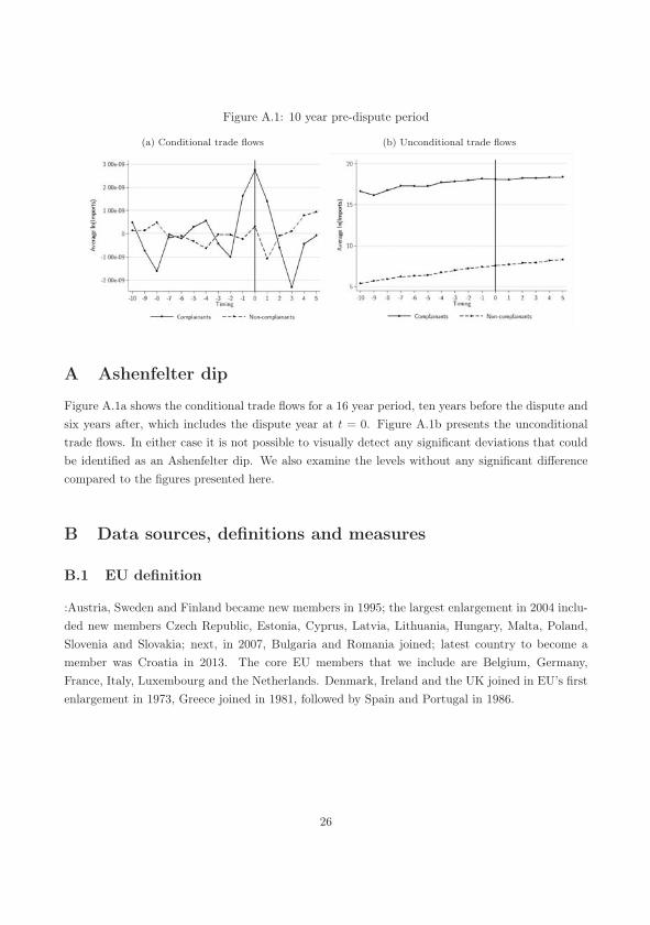
Figure A.1: 10 year pre-dispute period

(a) Conditional trade flows (b) Unconditional trade flows

A Ashenfelter dip

Figure A.1a shows the conditional trade flows for a 16 year period, ten years before the dispute andsix years after, which includes the dispute year at t = 0. Figure A.1b presents the unconditionaltrade flows. In either case it is not possible to visually detect any significant deviations that couldbe identified as an Ashenfelter dip. We also examine the levels without any significant differencecompared to the figures presented here.

B Data sources, definitions and measures

B.1 EU definition

:Austria, Sweden and Finland became new members in 1995; the largest enlargement in 2004 inclu-ded new members Czech Republic, Estonia, Cyprus, Latvia, Lithuania, Hungary, Malta, Poland,Slovenia and Slovakia; next, in 2007, Bulgaria and Romania joined; latest country to become amember was Croatia in 2013. The core EU members that we include are Belgium, Germany,France, Italy, Luxembourg and the Netherlands. Denmark, Ireland and the UK joined in EU’s firstenlargement in 1973, Greece joined in 1981, followed by Spain and Portugal in 1986.

26

Table B.1: EU timeline

In the analysis Time member countries

Main EU Pre-1995 Italy (1958), Ireland (1973),

Belgium (1958), Denmark

(1973), France (1958),

Germany (1958), Greece

(1981), Spain (1986), UK

(1973), Luxembourg (1958),

Portugal (1986), Netherlands

(1958)

Removed

First enlargement (1995) Sweden, Finland, Austria

Second enlargement (2004) Cyprus, Czech Republic,

Estonia, Hungary,

Latvia, Lithuania, Malta,

Poland, Slovakia, Slovenia

Third enlargement (2007) Bulgaria, Romania

2013 Croatia

27

ESSAY V

Figure A.1: 10 year pre-dispute period

(a) Conditional trade flows (b) Unconditional trade flows

A Ashenfelter dip

Figure A.1a shows the conditional trade flows for a 16 year period, ten years before the dispute andsix years after, which includes the dispute year at t = 0. Figure A.1b presents the unconditionaltrade flows. In either case it is not possible to visually detect any significant deviations that couldbe identified as an Ashenfelter dip. We also examine the levels without any significant differencecompared to the figures presented here.

B Data sources, definitions and measures

B.1 EU definition

:Austria, Sweden and Finland became new members in 1995; the largest enlargement in 2004 inclu-ded new members Czech Republic, Estonia, Cyprus, Latvia, Lithuania, Hungary, Malta, Poland,Slovenia and Slovakia; next, in 2007, Bulgaria and Romania joined; latest country to become amember was Croatia in 2013. The core EU members that we include are Belgium, Germany,France, Italy, Luxembourg and the Netherlands. Denmark, Ireland and the UK joined in EU’s firstenlargement in 1973, Greece joined in 1981, followed by Spain and Portugal in 1986.

26

Table B.1: EU timeline

In the analysis Time member countries

Main EU Pre-1995 Italy (1958), Ireland (1973),

Belgium (1958), Denmark

(1973), France (1958),

Germany (1958), Greece

(1981), Spain (1986), UK

(1973), Luxembourg (1958),

Portugal (1986), Netherlands

(1958)

Removed

First enlargement (1995) Sweden, Finland, Austria

Second enlargement (2004) Cyprus, Czech Republic,

Estonia, Hungary,

Latvia, Lithuania, Malta,

Poland, Slovakia, Slovenia

Third enlargement (2007) Bulgaria, Romania

2013 Croatia

27

Figure B.2: Time it takes to reach a settlement: days from consultation tonotification

Figure B.1: Trade flows for removed EU members relative to EU-12

28

C Conditional trade flows

Figure C.1 shows the conditional trade flows for complainants and non-complainants, respecti-vely. Note that the apparent unstable trade flows between the respondent markets and the controlmarkets is actually very small fluctuations that become exaggerated due to the scale of the y-axis.

Figure C.1: Conditional trade flows

(a) Complainants (b) Non-complainants

29

ESSAY V

Figure B.2: Time it takes to reach a settlement: days from consultation tonotification

Figure B.1: Trade flows for removed EU members relative to EU-12

28

C Conditional trade flows

Figure C.1 shows the conditional trade flows for complainants and non-complainants, respecti-vely. Note that the apparent unstable trade flows between the respondent markets and the controlmarkets is actually very small fluctuations that become exaggerated due to the scale of the y-axis.

Figure C.1: Conditional trade flows

(a) Complainants (b) Non-complainants

29

D First difference regressions

Applying a first difference transformation on our data implies a slightly different interpretation ofthe coefficients. Let t = 0, . . . , T so that dispute happens for r = 1 in t > t0. Also, let τ = I (t > t0)

then a standard DD equation with log-transformed imports is:

log yi,t = α+ γgi + βτt + δτtgi + `′xi

Taking differences in t instead yields the import growth rate,

Δt log yi,t = Δtα+Δtγgi + `′xi︸︷︷︸

=0

+βΔtτt + δΔ(τtri) .

Since the terms α , γgi and `′xi are constant in t, the differenced terms become zero. The time

dummy τ is β is for the treatment period, zero otherwise and δ is for the treatment group inthe treatment period, zero otherwise. In this specification, we can therefore control for a generalconstant growth rate by adding a constant, α to the equation and a group-specific growth rate effectby adding gi. We can also add time-invariant exporter-specific effects, xi, that could also affectgrowth rate. We also introduce year-specific δ so that we instead estimate incremental treatmenteffects, in log-levels, in period t, thereby accounting for shift-level effects rather than growth rateeffects. That is, if we only used a single post-dispute period, then we would impose the restrictionthat a dispute had growth rate effects. Hence, differencing allow us to estimate DD while accountingfor heterogeneous growth rates:

θ‘xi

Δt log yi,t = α+ θ‘xi + βτt + gi

T∑u>to

δI (t = u) + θ‘xi.

30

Tab

leD

.1:

Fir

stD

iffer

ence

plac

ebo

test

(a)

Adj

udic

ated

disp

utes

(1)

(2)

(3)

All

adju

dica

ted

Com

plai

nant

sN

on-c

ompl

aina

nts

DD

(T-2

)0.

01-0

.00

0.06

(0.0

4)(0

.06)

(0.0

4)

DD

(T-1

)-0

.06

-0.0

70.

01(0

.04)

(0.0

6)(0

.04)

DD

(T=

0)-0

.02

-0.0

70.

04(0

.04)

(0.0

6)(0

.04)

DD

(T+

1)0.

00-0

.01

0.06

(.)

(0.0

6)(0

.04)

DD

(T+

2)0.

010.

020.

07∗

(0.0

4)(0

.06)

(0.0

4)

DD

(T+

3)-0

.04

0.00

0.00

(0.0

4)(.

)(.

)

DD

(T+

4)-0

.02

0.00

0.03

(0.0

4)(0

.06)

(0.0

4)

DD

(T+

5)-0

.01

0.02

0.06

(0.0

4)(0

.06)

(0.0

4)N

3051

160

4302

7229

3074

4R

20.

030.

030.

03R

obus

tst

anda

rder

rors

.W

eigh

ted.

∗p<

0.10,∗∗

p<

0.05,∗∗

∗p<

0.001

(b)

Non

-adj

udic

ated

disp

utes

(1)

(2)

(3)

All

non-

adju

dica

ted

Com

plai

nant

sN

on-c

ompl

aina

nts

DD

(T-2

)0.

020.

15∗∗

0.03

(0.0

3)(0

.07)

(0.0

3)

DD

(T-1

)-0

.03

0.00

-0.0

1(0

.03)

(.)

(0.0

3)

DD

(T=

0)0.

06∗∗

0.07

0.07

∗∗

(0.0

3)(0

.07)

(0.0

3)

DD

(T+

1)-0

.00

0.08

0.01

(0.0

3)(0

.07)

(0.0

3)

DD

(T+

2)0.

08∗∗

0.18

∗∗0.

09∗∗

(0.0

3)(0

.07)

(0.0

3)

DD

(T+

3)-0

.02

0.03

-0.0

0(0

.03)

(0.0

7)(0

.03)

DD

(T+

4)-0

.03

0.07

-0.0

3(0

.03)

(0.0

7)(0

.03)

DD

(T+

5)0.

000.

070.

00(.

)(0

.07)

(.)

N29

1491

252

1408

2815

832

R2

0.03

0.03

0.03

Rob

ust

stan

dard

erro

rs.

Wei

ghte

d.∗p<

0.10,∗∗

p<

0.05,∗∗

∗p<

0.001

31

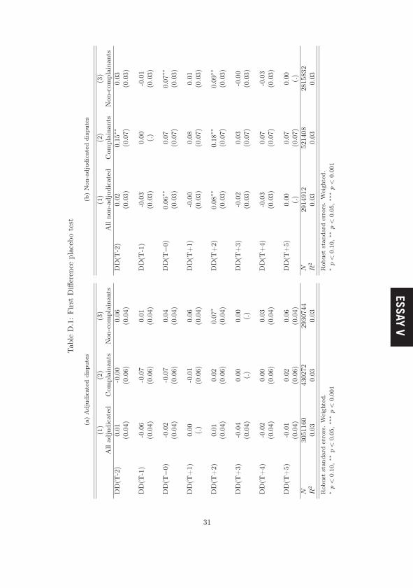
ESSAY V

D First difference regressions

Applying a first difference transformation on our data implies a slightly different interpretation ofthe coefficients. Let t = 0, . . . , T so that dispute happens for r = 1 in t > t0. Also, let τ = I (t > t0)

then a standard DD equation with log-transformed imports is:

log yi,t = α+ γgi + βτt + δτtgi + `′xi

Taking differences in t instead yields the import growth rate,

Δt log yi,t = Δtα+Δtγgi + `′xi︸︷︷︸

=0

+βΔtτt + δΔ(τtri) .

Since the terms α , γgi and `′xi are constant in t, the differenced terms become zero. The time

dummy τ is β is for the treatment period, zero otherwise and δ is for the treatment group inthe treatment period, zero otherwise. In this specification, we can therefore control for a generalconstant growth rate by adding a constant, α to the equation and a group-specific growth rate effectby adding gi. We can also add time-invariant exporter-specific effects, xi, that could also affectgrowth rate. We also introduce year-specific δ so that we instead estimate incremental treatmenteffects, in log-levels, in period t, thereby accounting for shift-level effects rather than growth rateeffects. That is, if we only used a single post-dispute period, then we would impose the restrictionthat a dispute had growth rate effects. Hence, differencing allow us to estimate DD while accountingfor heterogeneous growth rates:

θ‘xi

Δt log yi,t = α+ θ‘xi + βτt + gi

T∑u>to

δI (t = u) + θ‘xi.

30

Tab

leD

.1:

Fir

stD

iffer

ence

plac

ebo

test

(a)

Adj

udic

ated

disp

utes

(1)

(2)

(3)

All

adju

dica

ted

Com

plai

nant

sN

on-c

ompl

aina

nts

DD

(T-2

)0.

01-0

.00

0.06

(0.0

4)(0

.06)

(0.0

4)

DD

(T-1

)-0

.06

-0.0

70.

01(0

.04)

(0.0

6)(0

.04)

DD

(T=

0)-0

.02

-0.0

70.

04(0

.04)

(0.0

6)(0

.04)

DD

(T+

1)0.

00-0

.01

0.06

(.)

(0.0

6)(0

.04)

DD

(T+

2)0.

010.

020.

07∗

(0.0

4)(0

.06)

(0.0

4)

DD

(T+

3)-0

.04

0.00

0.00

(0.0

4)(.

)(.

)

DD

(T+

4)-0

.02

0.00

0.03

(0.0

4)(0

.06)

(0.0

4)

DD

(T+

5)-0

.01

0.02

0.06

(0.0

4)(0

.06)

(0.0

4)N

3051

160

4302

7229

3074

4R

20.

030.

030.

03R

obus

tst

anda

rder

rors

.W

eigh

ted.

∗p<

0.10,∗∗

p<

0.05,∗∗

∗p<

0.001

(b)

Non

-adj

udic

ated

disp

utes

(1)

(2)

(3)

All

non-

adju

dica

ted

Com

plai

nant

sN

on-c

ompl

aina

nts

DD

(T-2

)0.

020.

15∗∗

0.03

(0.0

3)(0

.07)

(0.0

3)

DD

(T-1

)-0

.03

0.00

-0.0

1(0

.03)

(.)

(0.0

3)

DD

(T=

0)0.

06∗∗

0.07

0.07

∗∗

(0.0

3)(0

.07)

(0.0

3)

DD

(T+

1)-0

.00

0.08

0.01

(0.0

3)(0

.07)

(0.0

3)

DD

(T+

2)0.

08∗∗

0.18

∗∗0.

09∗∗

(0.0

3)(0

.07)

(0.0

3)

DD

(T+

3)-0

.02

0.03

-0.0

0(0

.03)

(0.0

7)(0

.03)

DD

(T+

4)-0

.03

0.07

-0.0

3(0

.03)

(0.0

7)(0

.03)

DD

(T+

5)0.

000.

070.

00(.

)(0

.07)

(.)

N29

1491

252

1408

2815

832

R2

0.03

0.03

0.03

Rob

ust

stan

dard

erro

rs.

Wei

ghte

d.∗p<

0.10,∗∗

p<

0.05,∗∗

∗p<

0.001

31

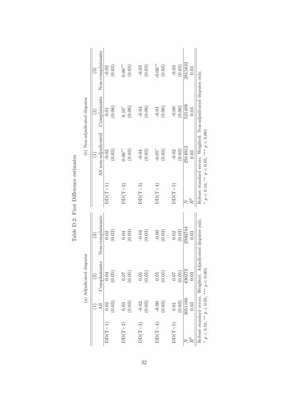
Tab

leD

.2:

Fir

stD

iffer

ence

esti

mat

es

(a)

Adj

udic

ated

disp

utes

(1)

(2)

(3)

All

Com

plai

nant

sN

on-c

ompl

aina

nts

DD

(T+

1)0.

020.

040.

02(0

.03)

(0.0

5)(0

.03)

DD

(T+

2)0.

030.

070.

04(0

.03)

(0.0

5)(0

.03)

DD

(T+

3)-0

.02

0.05

-0.0

4(0

.03)

(0.0

5)(0

.03)

DD

(T+

4)-0

.00

0.05

-0.0

0(0

.03)

(0.0

5)(0

.03)

DD

(T+

5)0.

010.

070.

02(0

.03)

(0.0

5)(0

.03)

N30

5116

043

0272

2930

744

R2

0.03

0.03

0.03

Rob

ust

stan

dard

erro

rs.

Wei

ghte

d.A

djud

icat

eddi

sput

eson

ly.

∗p<

0.10,∗∗

p<

0.05,∗∗

∗p<

0.001

(b)

Non

-adj

udic

ated

disp

utes

(1)

(2)

(3)

All

non-

adju

dica

ted

Com

plai

nant

sN

on-c

ompl

aina

nts

DD

(T+

1)-0

.02

0.01

-0.0

2(0

.03)

(0.0

6)(0

.03)

DD

(T+

2)0.

06∗∗

0.10

∗0.

06∗∗

(0.0

3)(0

.06)

(0.0

3)

DD

(T+

3)-0

.04

-0.0

4-0

.03

(0.0

3)(0

.06)

(0.0

3)

DD

(T+

4)-0

.05∗

-0.0

1-0

.06∗

∗

(0.0

3)(0

.06)

(0.0

3)

DD

(T+

5)-0

.02

-0.0

0-0

.03

(0.0

3)(0

.06)

(0.0

3)N

2914

912

5214

0828

1583

2R

20.

030.

030.

03R

obus

tst

anda

rder

rors

.W

eigh

ted.

Non

-adj

udic

ated

disp

utes

only

.∗p<

0.10,∗∗

p<

0.05,∗∗

∗p<

0.001

32

Figure E.1: Dispute-specific DD estimates

E Robustness

Because disputes are rather heterogeneous there could be large variation in the dispute effects forindividual disputes. For that reason we estimated two-period DD coefficients for each dispute, withrelevant controls, using our secondary control markets and combined them in Figure E.1. Thecoefficients in Figure E.1 seem to linger around zero but the standard deviation is undeniably largeof around 0.73 with a mean dispute effect of -0.013.

F Placebo tests

Below follows relevant placebo regressions to test the validity of pre-dispute trends between respon-dents’ import markets and primary and secondary control markets, including “placebo” disputetests between the primary and secondary control markets to examine potential spillover effects.The base year in all specifications is the first applicable pre-dispute year, T − 3.

33

ESSAY V

Tab

leD

.2:

Fir

stD

iffer

ence

esti

mat

es

(a)

Adj

udic

ated

disp

utes

(1)

(2)

(3)

All

Com

plai

nant

sN

on-c

ompl

aina

nts

DD

(T+

1)0.

020.

040.

02(0

.03)

(0.0

5)(0

.03)

DD

(T+

2)0.

030.

070.

04(0

.03)

(0.0

5)(0

.03)

DD

(T+

3)-0

.02

0.05

-0.0

4(0

.03)

(0.0

5)(0

.03)

DD

(T+

4)-0

.00

0.05

-0.0

0(0

.03)

(0.0

5)(0

.03)

DD

(T+

5)0.

010.

070.

02(0

.03)

(0.0

5)(0

.03)

N30

5116

043

0272

2930

744

R2

0.03

0.03

0.03

Rob

ust

stan

dard

erro

rs.

Wei

ghte

d.A

djud

icat

eddi

sput

eson

ly.

∗p<

0.10,∗∗

p<

0.05,∗∗

∗p<

0.001

(b)

Non

-adj

udic

ated

disp

utes

(1)

(2)

(3)

All

non-

adju

dica

ted

Com

plai

nant

sN

on-c

ompl

aina

nts

DD

(T+

1)-0

.02

0.01

-0.0

2(0

.03)

(0.0

6)(0

.03)

DD

(T+

2)0.

06∗∗

0.10

∗0.

06∗∗

(0.0

3)(0

.06)

(0.0

3)

DD

(T+

3)-0

.04

-0.0

4-0

.03

(0.0

3)(0

.06)

(0.0

3)

DD

(T+

4)-0

.05∗

-0.0

1-0

.06∗

∗

(0.0

3)(0

.06)

(0.0

3)

DD

(T+

5)-0

.02

-0.0

0-0

.03

(0.0

3)(0

.06)

(0.0

3)N

2914

912

5214

0828

1583

2R

20.

030.

030.

03R

obus

tst

anda

rder

rors

.W

eigh

ted.

Non

-adj

udic

ated

disp

utes

only

.∗p<

0.10,∗∗

p<

0.05,∗∗

∗p<

0.001

32

Figure E.1: Dispute-specific DD estimates

E Robustness

Because disputes are rather heterogeneous there could be large variation in the dispute effects forindividual disputes. For that reason we estimated two-period DD coefficients for each dispute, withrelevant controls, using our secondary control markets and combined them in Figure E.1. Thecoefficients in Figure E.1 seem to linger around zero but the standard deviation is undeniably largeof around 0.73 with a mean dispute effect of -0.013.

F Placebo tests

Below follows relevant placebo regressions to test the validity of pre-dispute trends between respon-dents’ import markets and primary and secondary control markets, including “placebo” disputetests between the primary and secondary control markets to examine potential spillover effects.The base year in all specifications is the first applicable pre-dispute year, T − 3.

33

Tab

leF.1

:P

rim

ary

cont

rolm

arke

ts:

Pla

cebo

test

s

(a)

Adj

udic

ated

disp

utes

(1)

(2)

(3)

All

adju

dica

ted

Com

plai

nant

sN

on-c

ompl

aina

nts

DD

(T-2

)-0

.03

0.03

-0.0

6(0

.09)

(0.3

2)(0

.09)

DD

(T-1

)-0

.07

0.34

-0.1

0(0

.09)

(0.3

4)(0

.09)

DD

(T=

0)-0

.14

-0.4

0-0

.11

(0.0

9)(0

.27)

(0.1

0)

DD

(T+

1)-0

.13

-0.5

3∗-0

.09

(0.0

9)(0

.28)

(0.0

9)

DD

(T+

2)-0

.21∗

∗-0

.51∗

-0.2

1∗∗

(0.0

9)(0

.28)

(0.1

0)

DD

(T+

3)-0

.24∗

∗-0

.46

-0.2

4∗∗

(0.0

9)(0

.30)

(0.1

0)

DD

(T+

4)-0

.17∗

-0.7

0∗∗

-0.1

5(0

.10)

(0.3

3)(0

.11)

DD

(T+

5)-0

.31∗

∗-0

.74∗

-0.2

8∗∗

(0.1

0)(0

.39)

(0.1

1)N

3131

235

1366

6629

9453

4R

20.

800.

880.

79R

obus

tst

anda

rder

rors

.W

eigh

ted.

∗p<

0.10,∗∗

p<

0.05,∗∗

∗p<

0.001

(b)

Non

-adj

udic

ated

disp

utes

(1)

(2)

(3)

All

non-

adju

dica

ted

Com

plai

nant

sN

on-c

ompl

aina

nts

DD

(T-2

)-0

.04

0.20

-0.0

7(0

.09)

(0.3

9)(0

.10)

DD

(T-1

)-0

.16∗

0.19

-0.2

1∗∗

(0.0

9)(0

.40)

(0.1

0)

DD

(T=

0)-0

.10

-0.0

1-0

.14

(0.0

9)(0

.40)

(0.1

0)

DD

(T+

1)-0

.04

-0.0

2-0

.05

(0.0

9)(0

.40)

(0.1

0)

DD

(T+

2)0.

05-0

.06

0.05

(0.0

9)(0

.40)

(0.1

0)

DD

(T+

3)0.

010.

09-0

.01

(0.0

9)(0

.40)

(0.1

0)

DD

(T+

4)0.

040.

140.

01(0

.09)

(0.4

1)(0

.10)

DD

(T+

5)0.

000.

080.

01(0

.10)

(0.4

3)(0

.11)

N28

4528

511

2441

2732

803

R2

0.80

0.88

0.79

Rob

ust

stan

dard

erro

rs.

Wei

ghte

d.∗p<

0.10,∗∗

p<

0.05,∗∗

∗p<

0.001

Tab

leF.2

:Sp

illov

er.

Pla

cebo

test

s

(a)

Adj

udic

ated

disp

utes

(1)

(2)

(3)

All

adju

dica

ted

Com

plai

nant

sN

on-c

ompl

aina

nts

DD

(T-2

)0.

030.

11∗∗

0.02

(0.0

3)(0

.05)

(0.0

3)

DD

(T-1

)0.

010.

060.

01(0

.03)

(0.0

5)(0

.03)

DD

(T=

0)0.

040.

09∗

0.03

(0.0

3)(0

.05)

(0.0

3)

DD

(T+

1)0.

08∗∗

0.15

∗∗0.

08∗∗

(0.0

3)(0

.05)

(0.0

3)

DD

(T+

2)0.

13∗∗

∗0.

23∗∗

∗0.

13∗∗

∗

(0.0

3)(0

.05)

(0.0

3)

DD

(T+

3)0.

14∗∗

∗0.

30∗∗

∗0.

13∗∗

∗

(0.0

3)(0

.06)

(0.0

3)

DD

(T+

4)0.

17∗∗

∗0.

39∗∗

∗0.

16∗∗

∗

(0.0

3)(0

.06)

(0.0

3)

DD

(T+

5)0.

21∗∗

∗0.

41∗∗

∗0.

20∗∗

∗

(0.0

3)(0

.06)

(0.0

3)N

3432

555

4840

4932

9708

7R

20.

800.

900.

79R

obus

tst

anda

rder

rors

.W

eigh

ted.

∗p<

0.10,∗∗

p<

0.05,∗∗

∗p<

0.001

(b)

Non

-adj

udic

ated

disp

utes

(1)

(2)

(3)

All

non-

adju

dica

ted

Com

plai

nant

sN

on-c

ompl

aina

nts

DD

(T-2

)0.

030.

010.

03(0

.03)

(0.0

6)(0

.03)

DD

(T-1

)0.

02-0

.01

0.02

(0.0

2)(0

.06)

(0.0

3)

DD

(T=

0)0.

09∗∗

∗-0

.06

0.08

∗∗

(0.0

3)(0

.06)

(0.0

3)

DD

(T+

1)0.

10∗∗

∗-0

.06

0.10

∗∗∗

(0.0

3)(0

.06)

(0.0

3)

DD

(T+

2)0.

18∗∗

∗0.

010.

17∗∗

∗

(0.0

3)(0

.06)

(0.0

3)

DD

(T+

3)0.

19∗∗

∗-0

.01

0.19

∗∗∗

(0.0

3)(0

.07)

(0.0

3)

DD

(T+

4)0.

19∗∗

∗-0

.05

0.18

∗∗∗

(0.0

3)(0

.07)

(0.0

3)

DD

(T+

5)0.

20∗∗

∗-0

.06

0.18

∗∗∗

(0.0

3)(0

.07)

(0.0

3)N

3279

276

5865

7331

6781

1R

20.

800.

870.

79R

obus

tst

anda

rder

rors

.W

eigh

ted.

∗p<

0.10,∗∗

p<

0.05,∗∗

∗p<

0.001

ESSAY V

Tab

leF.2

:Sp

illov

er.

Pla

cebo

test

s

(a)

Adj

udic

ated

disp

utes

(1)

(2)

(3)

All

adju

dica

ted

Com

plai

nant

sN

on-c

ompl

aina

nts

DD

(T-2

)0.

030.

11∗∗

0.02

(0.0

3)(0

.05)

(0.0

3)

DD

(T-1

)0.

010.

060.

01(0

.03)

(0.0

5)(0

.03)

DD

(T=

0)0.

040.

09∗

0.03

(0.0

3)(0

.05)

(0.0

3)

DD

(T+

1)0.

08∗∗

0.15

∗∗0.

08∗∗

(0.0

3)(0

.05)

(0.0

3)

DD

(T+

2)0.

13∗∗

∗0.

23∗∗

∗0.

13∗∗

∗

(0.0

3)(0

.05)

(0.0

3)

DD

(T+

3)0.

14∗∗

∗0.

30∗∗

∗0.

13∗∗

∗

(0.0

3)(0

.06)

(0.0

3)

DD

(T+

4)0.

17∗∗

∗0.

39∗∗

∗0.

16∗∗

∗

(0.0

3)(0

.06)

(0.0

3)

DD

(T+

5)0.

21∗∗

∗0.

41∗∗

∗0.

20∗∗

∗

(0.0

3)(0

.06)

(0.0

3)N

3432

555

4840

4932

9708

7R

20.

800.

900.

79R

obus

tst

anda

rder

rors

.W

eigh

ted.

∗p<

0.10,∗∗

p<

0.05,∗∗

∗p<

0.001

(b)

Non

-adj

udic

ated

disp

utes

(1)

(2)

(3)

All

non-

adju

dica

ted

Com

plai

nant

sN

on-c

ompl

aina

nts

DD

(T-2

)0.

030.

010.

03(0

.03)

(0.0

6)(0

.03)

DD

(T-1

)0.

02-0

.01

0.02

(0.0

2)(0

.06)

(0.0

3)

DD

(T=

0)0.

09∗∗

∗-0

.06

0.08

∗∗

(0.0

3)(0

.06)

(0.0

3)

DD

(T+

1)0.

10∗∗

∗-0

.06

0.10

∗∗∗

(0.0

3)(0

.06)

(0.0

3)

DD

(T+

2)0.

18∗∗

∗0.

010.

17∗∗

∗

(0.0

3)(0

.06)

(0.0

3)

DD

(T+

3)0.

19∗∗

∗-0

.01

0.19

∗∗∗

(0.0

3)(0

.07)

(0.0

3)

DD

(T+

4)0.

19∗∗

∗-0

.05

0.18

∗∗∗

(0.0

3)(0

.07)

(0.0

3)

DD

(T+

5)0.

20∗∗

∗-0

.06

0.18

∗∗∗

(0.0

3)(0

.07)

(0.0

3)N

3279

276

5865

7331

6781

1R

20.

800.

870.

79R

obus

tst

anda

rder

rors

.W

eigh

ted.

∗p<

0.10,∗∗

p<

0.05,∗∗

∗p<

0.001

Tab

leF.3

:Se

cond

ary

cont

rolm

arke

ts:

Pla

cebo

test

s

(a)

Adj

udic

ated

disp

utes

(1)

(2)

(3)

All

adju

dica

ted

Com

plai

nant

sN

on-c

ompl

aina

nts

DD

(T-2

)-0

.03

-0.1

4-0

.02

(0.0

8)(0

.14)

(0.0

8)

DD

(T-1

)0.

05-0

.09

0.06

(0.0

8)(0

.13)

(0.0

8)

DD

(T=

0)0.

00-0

.29∗

∗0.

02(0

.08)

(0.1

3)(0

.08)

DD

(T+

1)0.

08-0

.47∗

∗∗0.

11(0

.08)

(0.1

4)(0

.09)

DD

(T+

2)0.

06-0

.38∗

∗0.

09(0

.09)

(0.1

4)(0

.09)

DD

(T+

3)-0

.01

-0.4

2∗∗

0.02

(0.1

0)(0

.16)

(0.1

0)

DD

(T+

4)0.

10-0

.64∗

∗∗0.

14(0

.11)

(0.1

8)(0

.11)

DD

(T+

5)0.

03-0

.52∗

∗0.

07(0

.12)

(0.1

8)(0

.12)

N39

5851

3497

7739

4615

R2

0.88

0.90

0.88

Rob

ust

stan

dard

erro

rs.

Wei

ghte

d.∗p<

0.10,∗∗

p<

0.05,∗∗

∗p<

0.001

(b)

Non

-adj

udic

ated

disp

utes

(1)

(2)

(3)

All

non-

adju

dica

ted

Com

plai

nant

sN

on-c

ompl

aina

nts

DD

(T-2

)0.

030.

010.

03(0

.03)

(0.0

6)(0

.03)

DD

(T-1

)0.

02-0

.01

0.02

(0.0

2)(0

.06)

(0.0

3)

DD

(T=

0)0.

09∗∗

∗-0

.06

0.08

∗∗

(0.0

3)(0

.06)

(0.0

3)

DD

(T+

1)0.

10∗∗

∗-0

.06

0.10

∗∗∗

(0.0

3)(0

.06)

(0.0

3)

DD

(T+

2)0.

18∗∗

∗0.

010.

17∗∗

∗

(0.0

3)(0

.06)

(0.0

3)

DD

(T+

3)0.

19∗∗

∗-0

.01

0.19

∗∗∗

(0.0

3)(0

.07)

(0.0

3)

DD

(T+

4)0.

19∗∗

∗-0

.05

0.18

∗∗∗

(0.0

3)(0

.07)

(0.0

3)

DD

(T+

5)0.

20∗∗

∗-0

.06

0.18

∗∗∗

(0.0

3)(0

.07)

(0.0

3)N

3279

276

5865

7331

6781

1R

20.

800.

870.

79R

obus

tst

anda

rder

rors

.W

eigh

ted.

∗p<

0.10,∗∗

p<

0.05,∗∗

∗p<

0.001

Tab

leF.4

:D

Des

tim

ates

rega

rdle

ssof

outc

ome.

Pla

cebo

effec

ts

(a)

Res

pond

ents

(1)

(2)

(3)

All

Com

plai

nant

sN

on-c

ompl

aina

nts

DD

(T-2

)0.

02-0

.09

0.02

(0.0

6)(0

.10)

(0.0

6)

DD

(T-1

)0.

01-0

.11

0.02

(0.0

6)(0

.09)

(0.0

6)

DD

(T=

0)0.

08-0

.29∗

∗0.

10∗

(0.0

6)(0

.09)

(0.0

6)

DD

(T+

1)0.

16∗∗

-0.4

3∗∗∗

0.18

∗∗

(0.0

6)(0

.09)

(0.0

6)

DD

(T+

2)0.

27∗∗

∗-0

.49∗

∗∗0.

30∗∗

∗

(0.0

6)(0

.10)

(0.0

6)

DD

(T+

3)0.

26∗∗

∗-0

.55∗

∗∗0.

29∗∗

∗

(0.0

6)(0

.10)

(0.0

7)

DD

(T+

4)0.

34∗∗

∗-0

.61∗

∗∗0.

38∗∗

∗

(0.0

7)(0

.12)

(0.0

7)

DD

(T+

5)0.

35∗∗

∗-0

.69∗

∗∗0.

39∗∗

∗

(0.0

7)(0

.12)

(0.0

7)N

9121

0382

5916

9098

53R

20.

860.

880.

86R

obus

tst

anda

rder

rors

.W

eigh

ted.

∗p<

0.10,∗∗

p<

0.05,∗∗

∗p<

0.001

(b)

Pri

mar

yco

ntro

lm

arke

ts,sp

illov

er.

(1)

(2)

(3)

All

Com

plai

nant

sN

on-c

ompl

aina

nts

DD

(T-2

)0.

030.

080.

02(0

.02)

(0.0

5)(0

.02)

DD

(T-1

)0.

010.

09∗

0.01

(0.0

2)(0

.05)

(0.0

2)

DD

(T=

0)0.

05∗∗

0.04

0.05

∗∗

(0.0

2)(0

.05)

(0.0

2)

DD

(T+

1)0.

08∗∗

∗0.

060.

08∗∗

∗

(0.0

2)(0

.05)

(0.0

2)

DD

(T+

2)0.

14∗∗

∗0.

17∗∗

∗0.

14∗∗

∗

(0.0

2)(0

.05)

(0.0

2)

DD

(T+

3)0.

15∗∗

∗0.

17∗∗

∗0.

15∗∗

∗

(0.0

2)(0

.05)

(0.0

2)

DD

(T+

4)0.

16∗∗

∗0.

22∗∗

∗0.

16∗∗

∗

(0.0

2)(0

.05)

(0.0

2)

DD

(T+

5)0.

18∗∗

∗0.

20∗∗

∗0.

17∗∗

∗

(0.0

2)(0

.05)

(0.0

2)N

6711

831

1070

640

6464

898

R2

0.80

0.88

0.79

Rob

ust

stan

dard

erro

rs.

Wei

ghte

d.A

lldi

sput

es.

∗p<

0.10,∗∗

p<

0.05,∗∗

∗p<

0.001

ESSAY V

Tab

leF.4

:D

Des

tim

ates

rega

rdle

ssof

outc

ome.

Pla

cebo

effec

ts

(a)

Res

pond

ents

(1)

(2)

(3)

All

Com

plai

nant

sN

on-c

ompl

aina

nts

DD

(T-2

)0.

02-0

.09

0.02

(0.0

6)(0

.10)

(0.0

6)

DD

(T-1

)0.

01-0

.11

0.02

(0.0

6)(0

.09)

(0.0

6)

DD

(T=

0)0.

08-0

.29∗

∗0.

10∗

(0.0

6)(0

.09)

(0.0

6)

DD

(T+

1)0.

16∗∗

-0.4

3∗∗∗

0.18

∗∗

(0.0

6)(0

.09)

(0.0

6)

DD

(T+

2)0.

27∗∗

∗-0

.49∗

∗∗0.

30∗∗

∗

(0.0

6)(0

.10)

(0.0

6)

DD

(T+

3)0.

26∗∗

∗-0

.55∗

∗∗0.

29∗∗

∗

(0.0

6)(0

.10)

(0.0

7)

DD

(T+

4)0.

34∗∗

∗-0

.61∗

∗∗0.

38∗∗

∗

(0.0

7)(0

.12)

(0.0

7)

DD

(T+

5)0.

35∗∗

∗-0

.69∗

∗∗0.

39∗∗

∗

(0.0

7)(0

.12)

(0.0

7)N

9121

0382

5916

9098

53R

20.

860.

880.

86R

obus

tst

anda

rder

rors

.W

eigh

ted.

∗p<

0.10,∗∗

p<

0.05,∗∗

∗p<

0.001

(b)

Pri

mar

yco

ntro

lm

arke

ts,sp

illov

er.

(1)

(2)

(3)

All

Com

plai

nant

sN

on-c

ompl

aina

nts

DD

(T-2

)0.

030.

080.

02(0

.02)

(0.0

5)(0

.02)

DD

(T-1

)0.

010.

09∗

0.01

(0.0

2)(0

.05)

(0.0

2)

DD

(T=

0)0.

05∗∗

0.04

0.05

∗∗

(0.0

2)(0

.05)

(0.0

2)

DD

(T+

1)0.

08∗∗

∗0.

060.

08∗∗

∗

(0.0

2)(0

.05)

(0.0

2)

DD

(T+

2)0.

14∗∗

∗0.

17∗∗

∗0.

14∗∗

∗

(0.0

2)(0

.05)

(0.0

2)

DD

(T+

3)0.

15∗∗

∗0.

17∗∗

∗0.

15∗∗

∗

(0.0

2)(0

.05)

(0.0

2)

DD

(T+

4)0.

16∗∗

∗0.

22∗∗

∗0.

16∗∗

∗

(0.0

2)(0

.05)

(0.0

2)

DD

(T+

5)0.

18∗∗

∗0.

20∗∗

∗0.

17∗∗

∗

(0.0

2)(0

.05)

(0.0

2)N

6711

831

1070

640

6464

898

R2

0.80

0.88

0.79

Rob

ust

stan

dard

erro

rs.

Wei

ghte

d.A

lldi

sput

es.

∗p<

0.10,∗∗

p<

0.05,∗∗

∗p<

0.001

G Supplementary results

Table G.1: DD estimates using primary control markets.

(a) Adjudicated disputes

(1) (2) (3)All adjudicated Complainants Non-complainants

DD(T+1) -0.06 -0.51∗∗ -0.02(0.06) (0.19) (0.07)

DD(T+2) -0.14∗∗ -0.49∗∗ -0.14∗

(0.07) (0.18) (0.07)

DD(T+3) -0.17∗∗ -0.44∗∗ -0.16∗∗

(0.07) (0.20) (0.07)

DD(T+4) -0.10 -0.66∗∗ -0.07(0.07) (0.23) (0.08)

DD(T+5) -0.24∗∗ -0.70∗∗ -0.20∗∗

(0.08) (0.29) (0.08)N 3131235 136666 2994534R2 0.80 0.88 0.79Robust standard errors. Weighted.∗ p < 0.10, ∗∗ p < 0.05, ∗∗∗ p < 0.001

(1) (2) (3)All non-adjudicated Complainants Non-complainants

DD(T+1) 0.03 -0.11 0.06(0.06) (0.18) (0.07)

DD(T+2) 0.13∗ -0.16 0.16∗∗

(0.07) (0.17) (0.07)

DD(T+3) 0.09 -0.00 0.10(0.07) (0.17) (0.08)

DD(T+4) 0.12∗ 0.05 0.12(0.07) (0.18) (0.08)

DD(T+5) 0.08 -0.01 0.12(0.07) (0.22) (0.08)

N 2845285 112441 2732803R2 0.80 0.88 0.79Robust standard errors. Weighted.∗ p < 0.10, ∗∗ p < 0.05, ∗∗∗ p < 0.001

(b) Non-adjudicated disputes

Tab

leG

.2:

Agr

icul

ture

:P

lace

bote

sts

(a)

Adj

udic

ated

disp

utes

(1)

(2)

(3)

All

adju

dica

ted

Com

plai

nant

sN

on-c

ompl

aina

nts

DD

(T-2

)0.

270.

230.

27(0

.18)

(0.4

2)(0

.18)

DD

(T-1

)0.

280.

390.

28(0

.18)

(0.4

0)(0

.18)

DD

(T=

0)0.

63∗∗

∗0.

120.

64∗∗

∗

(0.1

9)(0

.42)

(0.1

9)

DD

(T+

1)0.

41∗∗

-0.0

00.

42∗∗

(0.1

9)(0

.45)

(0.1

9)

DD

(T+

2)0.

41∗∗

-0.3

50.

43∗∗

(0.1

9)(0

.43)

(0.1

9)

DD

(T+

3)0.

54∗∗

-0.6

90.

56∗∗

(0.2

0)(0

.50)

(0.2

0)

DD

(T+

4)0.

42∗∗

-1.1

9∗∗

0.44

∗∗

(0.2

1)(0

.48)

(0.2

1)

DD

(T+

5)0.

60∗∗

-1.0

4∗∗

0.62

∗∗

(0.2

2)(0

.46)

(0.2

2)N

1548

9614

3427

1546

98R

20.

790.

800.

79R

obus

tst

anda

rder

rors

.W

eigh

ted.

∗p<

0.10,∗∗

p<

0.05,∗∗

∗p<

0.001

(b)

Non

-adj

udic

ated

disp

utes

(1)

(2)

(3)

All

adju

dica

ted

Com

plai

nant

sN

on-c

ompl

aina

nts

DD

(T-2

)-0

.07

-0.2

3-0

.06

(0.1

4)(0

.37)

(0.1

4)

DD

(T-1

)-0

.11

-0.2

8-0

.11

(0.1

4)(0

.40)

(0.1

4)

DD

(T=

0)-0

.31∗

∗-0

.39

-0.3

2∗∗

(0.1

4)(0

.38)

(0.1

4)

DD

(T+

1)-0

.11

-0.4

8-0

.11

(0.1

4)(0

.40)

(0.1

4)

DD

(T+

2)-0

.30∗

∗-0

.34

-0.3

2∗∗

(0.1

4)(0

.38)

(0.1

4)

DD

(T+

3)-0

.32∗

∗-0

.72∗

-0.3

3∗∗

(0.1

4)(0

.42)

(0.1

5)

DD

(T+

4)-0

.09

-0.5

9-0

.10

(0.1

5)(0

.46)

(0.1

5)

DD

(T+

5)-0

.19

-1.1

2∗∗

-0.1

9(0

.15)

(0.4

4)(0

.15)

N41

5979

3930

9941

5597

R2

0.78

0.78

0.78

Rob

ust

stan

dard

erro

rs.

Wei

ghte

d.∗p<

0.10,∗∗

p<

0.05,∗∗

∗p<

0.001

ESSAY V

Tab

leG

.2:

Agr

icul

ture

:P

lace

bote

sts

(a)

Adj

udic

ated

disp

utes

(1)

(2)

(3)

All

adju

dica

ted

Com

plai

nant

sN

on-c

ompl

aina

nts

DD

(T-2

)0.

270.

230.

27(0

.18)

(0.4

2)(0

.18)

DD

(T-1

)0.

280.

390.

28(0

.18)

(0.4

0)(0

.18)

DD

(T=

0)0.

63∗∗

∗0.

120.

64∗∗

∗

(0.1

9)(0

.42)

(0.1

9)

DD

(T+

1)0.

41∗∗

-0.0

00.

42∗∗

(0.1

9)(0

.45)

(0.1

9)

DD

(T+

2)0.

41∗∗

-0.3

50.

43∗∗

(0.1

9)(0

.43)

(0.1

9)

DD

(T+

3)0.

54∗∗

-0.6

90.

56∗∗

(0.2

0)(0

.50)

(0.2

0)

DD

(T+

4)0.

42∗∗

-1.1

9∗∗

0.44

∗∗

(0.2

1)(0

.48)

(0.2

1)

DD

(T+

5)0.

60∗∗

-1.0

4∗∗

0.62

∗∗

(0.2

2)(0

.46)

(0.2

2)N

1548

9614

3427

1546

98R

20.

790.

800.

79R

obus

tst

anda

rder

rors

.W

eigh

ted.

∗p<

0.10,∗∗

p<

0.05,∗∗

∗p<

0.001

(b)

Non

-adj

udic

ated

disp

utes

(1)

(2)

(3)

All

adju

dica

ted

Com

plai

nant

sN

on-c

ompl

aina

nts

DD

(T-2

)-0

.07

-0.2

3-0

.06

(0.1

4)(0

.37)

(0.1

4)

DD

(T-1

)-0

.11

-0.2

8-0

.11

(0.1

4)(0

.40)

(0.1

4)

DD

(T=

0)-0

.31∗

∗-0

.39

-0.3

2∗∗

(0.1

4)(0

.38)

(0.1

4)

DD

(T+

1)-0

.11

-0.4

8-0

.11

(0.1

4)(0

.40)

(0.1

4)

DD

(T+

2)-0

.30∗

∗-0

.34

-0.3

2∗∗

(0.1

4)(0

.38)

(0.1

4)

DD

(T+

3)-0

.32∗

∗-0

.72∗

-0.3

3∗∗

(0.1

4)(0

.42)

(0.1

5)

DD

(T+

4)-0

.09

-0.5

9-0

.10

(0.1

5)(0

.46)

(0.1

5)

DD

(T+

5)-0

.19

-1.1

2∗∗

-0.1

9(0

.15)

(0.4

4)(0

.15)

N41

5979

3930

9941

5597

R2

0.78

0.78

0.78

Rob

ust

stan

dard

erro

rs.

Wei

ghte

d.∗p<

0.10,∗∗

p<

0.05,∗∗

∗p<

0.001

Tab

leG

.3:

Agr

icul

ture

:D

Des

tim

ates

(a)

Adj

udic

ated

disp

utes

(1)

(2)

(3)

All

adju

dica

ted

Com

plai

nant

sN

on-c

ompl

aina

nts

DD

(T+

1)0.

02-0

.19

0.03

(0.1

4)(0

.30)

(0.1

5)

DD

(T+

2)0.

04-0

.54∗

∗0.

05(0

.15)

(0.2

6)(0

.15)

DD

(T+

3)0.

18-0

.88∗

∗0.

20(0

.15)

(0.3

6)(0

.15)

DD

(T+

4)0.

05-1

.37∗

∗∗0.

07(0

.16)

(0.3

3)(0

.17)

DD

(T+

5)0.

20-1

.23∗

∗∗0.

21(0

.18)

(0.3

1)(0

.18)

N15

4896

1434

2715

4698

R2

0.79

0.80

0.79

Rob

ust

stan

dard

erro

rs.

Wei

ghte

d.∗p<

0.10,∗∗

p<

0.05,∗∗

∗p<

0.001

(b)

Non

-adj

udic

ated

disp

utes

(1)

(2)

(3)

All

adju

dica

ted

Com

plai

nant

sN

on-c

ompl

aina

nts

DD

(T+

1)0.

04-0

.21

0.05

(0.1

0)(0

.24)

(0.1

0)

DD

(T+

2)-0

.15

-0.0

8-0

.16

(0.1

0)(0

.19)

(0.1

0)

DD

(T+

3)-0

.15

-0.4

4∗-0

.15

(0.1

0)(0

.26)

(0.1

0)

DD

(T+

4)0.

07-0

.32

0.07

(0.1

1)(0

.32)

(0.1

1)

DD

(T+

5)-0

.02

-0.8

5∗∗

-0.0

1(0

.11)

(0.2

7)(0

.11)

N41

5979

3930

9941

5597

R2

0.78

0.78

0.78

Rob

ust

stan

dard

erro

rs.

Wei

ghte

d.∗p<

0.10,∗∗

p<

0.05,∗∗

∗p<

0.001

Tab

leG

.4:

Agr

icul

ture

,spi

llove

r:P

lace

bote

sts

(a)

Adj

udic

ated

disp

utes

(1)

(2)

(3)

All

adju

dica

ted

Com

plai

nant

sN

on-c

ompl

aina

nts

DD

(T-2

)0.

070.

030.

09∗

(0.0

5)(0

.19)

(0.0

5)

DD

(T-1

)0.

15∗∗

0.26

0.15

∗∗

(0.0

5)(0

.18)

(0.0

5)

DD

(T=

0)0.

17∗∗

∗0.

42∗∗

0.18

∗∗∗

(0.0

5)(0

.19)

(0.0

5)

DD

(T+

1)0.

12∗∗

0.59

∗∗0.

13∗∗

(0.0

5)(0

.19)

(0.0

5)

DD

(T+

2)0.

13∗∗

0.71

∗∗∗

0.10

∗

(0.0

5)(0

.20)

(0.0

5)

DD

(T+

3)0.

13∗∗

0.98

∗∗∗

0.07

(0.0

5)(0

.20)

(0.0

6)

DD

(T+

4)0.

23∗∗

∗1.

00∗∗

∗0.

19∗∗

∗

(0.0

6)(0

.21)

(0.0

6)

DD

(T+

5)0.

24∗∗

∗1.

10∗∗

∗0.

20∗∗

∗

(0.0

6)(0

.22)

(0.0

6)N

5774

4816

1724

5589

80R

20.

760.

810.

75R

obus

tst

anda

rder

rors

.W

eigh

ted.

∗p<

0.10,∗∗

p<

0.05,∗∗

∗p<

0.001

(b)

Non

-adj

udic

ated

disp

utes

(1)

(2)

(3)

All

adju

dica

ted

Com

plai

nant

sN

on-c

ompl

aina

nts

DD

(T-2

)0.

040.

090.

03(0

.03)

(0.1

2)(0

.03)

DD

(T-1

)0.

07∗∗

0.12

0.06

∗

(0.0

3)(0

.12)

(0.0

3)

DD

(T=

0)0.

11∗∗

0.11

0.09

∗∗

(0.0

3)(0

.13)

(0.0

3)

DD

(T+

1)0.

09∗∗

0.18

0.08

∗∗

(0.0

3)(0

.12)

(0.0

3)

DD

(T+

2)0.

12∗∗

∗0.

29∗∗

0.10

∗∗

(0.0

4)(0

.13)

(0.0

4)

DD

(T+

3)0.

15∗∗

∗0.

37∗∗

0.13

∗∗∗

(0.0

4)(0

.13)

(0.0

4)

DD

(T+

4)0.

19∗∗

∗0.

34∗∗

0.15

∗∗∗

(0.0

4)(0

.13)

(0.0

4)

DD

(T+

5)0.

22∗∗

∗0.

39∗∗

0.21

∗∗∗

(0.0

4)(0

.14)

(0.0

4)N

1616

334

4274

5115

8162

1R

20.

770.

810.

76R

obus

tst

anda

rder

rors

.W

eigh

ted.

∗p<

0.10,∗∗

p<

0.05,∗∗

∗p<

0.001

ESSAY V

Tab

leG

.3:

Agr

icul

ture

:D

Des

tim

ates

(a)

Adj

udic

ated

disp

utes

(1)

(2)

(3)

All

adju

dica

ted

Com

plai

nant

sN

on-c

ompl

aina

nts

DD

(T+

1)0.

02-0

.19

0.03

(0.1

4)(0

.30)

(0.1

5)

DD

(T+

2)0.

04-0

.54∗

∗0.

05(0

.15)

(0.2

6)(0

.15)

DD

(T+

3)0.

18-0

.88∗

∗0.

20(0

.15)

(0.3

6)(0

.15)

DD

(T+

4)0.

05-1

.37∗

∗∗0.

07(0

.16)

(0.3

3)(0

.17)

DD

(T+

5)0.

20-1

.23∗

∗∗0.

21(0

.18)

(0.3

1)(0

.18)

N15

4896

1434

2715

4698

R2

0.79

0.80

0.79

Rob

ust

stan

dard

erro

rs.

Wei

ghte

d.∗p<

0.10,∗∗

p<

0.05,∗∗

∗p<

0.001

(b)

Non

-adj

udic

ated

disp

utes

(1)

(2)

(3)

All

adju

dica

ted

Com

plai

nant

sN

on-c

ompl

aina

nts

DD

(T+

1)0.

04-0

.21

0.05

(0.1

0)(0

.24)

(0.1

0)

DD

(T+

2)-0

.15

-0.0

8-0

.16

(0.1

0)(0

.19)

(0.1

0)

DD

(T+

3)-0

.15

-0.4

4∗-0

.15

(0.1

0)(0

.26)

(0.1

0)

DD

(T+

4)0.

07-0

.32

0.07

(0.1

1)(0

.32)

(0.1

1)

DD

(T+

5)-0

.02

-0.8

5∗∗

-0.0

1(0

.11)

(0.2

7)(0

.11)

N41

5979

3930

9941

5597

R2

0.78

0.78

0.78

Rob

ust

stan

dard

erro

rs.

Wei

ghte

d.∗p<

0.10,∗∗

p<

0.05,∗∗

∗p<

0.001

Tab

leG

.4:

Agr

icul

ture

,spi

llove

r:P

lace

bote

sts

(a)

Adj

udic

ated

disp

utes

(1)

(2)

(3)

All

adju

dica

ted

Com

plai

nant

sN

on-c

ompl

aina

nts

DD

(T-2

)0.

070.

030.

09∗

(0.0

5)(0

.19)

(0.0

5)

DD

(T-1

)0.

15∗∗

0.26

0.15

∗∗

(0.0

5)(0

.18)

(0.0

5)

DD

(T=

0)0.

17∗∗

∗0.

42∗∗

0.18

∗∗∗

(0.0

5)(0

.19)

(0.0

5)

DD

(T+

1)0.

12∗∗

0.59

∗∗0.

13∗∗

(0.0

5)(0

.19)

(0.0

5)

DD

(T+

2)0.

13∗∗

0.71

∗∗∗

0.10

∗

(0.0

5)(0

.20)

(0.0

5)

DD

(T+

3)0.

13∗∗

0.98

∗∗∗

0.07

(0.0

5)(0

.20)

(0.0

6)

DD

(T+

4)0.

23∗∗

∗1.

00∗∗

∗0.

19∗∗

∗

(0.0

6)(0

.21)

(0.0

6)

DD

(T+

5)0.

24∗∗

∗1.

10∗∗

∗0.

20∗∗

∗

(0.0

6)(0

.22)

(0.0

6)N

5774

4816

1724

5589

80R

20.

760.

810.

75R

obus

tst

anda

rder

rors

.W

eigh

ted.

∗p<

0.10,∗∗

p<

0.05,∗∗

∗p<

0.001

(b)

Non

-adj

udic

ated

disp

utes

(1)

(2)

(3)

All

adju

dica

ted

Com

plai

nant

sN

on-c

ompl

aina

nts

DD

(T-2

)0.

040.

090.

03(0

.03)

(0.1

2)(0

.03)

DD

(T-1

)0.

07∗∗

0.12

0.06

∗

(0.0

3)(0

.12)

(0.0

3)

DD

(T=

0)0.

11∗∗

0.11

0.09

∗∗

(0.0

3)(0

.13)

(0.0

3)

DD

(T+

1)0.

09∗∗

0.18

0.08

∗∗

(0.0

3)(0

.12)

(0.0

3)

DD

(T+

2)0.

12∗∗

∗0.

29∗∗

0.10

∗∗

(0.0

4)(0

.13)

(0.0

4)

DD

(T+

3)0.

15∗∗

∗0.

37∗∗

0.13

∗∗∗

(0.0

4)(0

.13)

(0.0

4)

DD

(T+

4)0.

19∗∗

∗0.

34∗∗

0.15

∗∗∗

(0.0

4)(0

.13)

(0.0

4)

DD

(T+

5)0.

22∗∗

∗0.

39∗∗

0.21

∗∗∗

(0.0

4)(0

.14)

(0.0

4)N

1616

334

4274

5115

8162

1R

20.

770.

810.

76R

obus

tst

anda

rder

rors

.W

eigh

ted.

∗p<

0.10,∗∗

p<

0.05,∗∗

∗p<

0.001

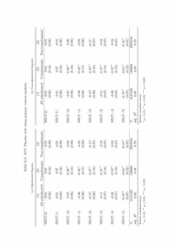
Tab

leG

.5:

AT

T:P

lace

bote

sts

usin

gpr

imar

yco

ntro

lmar

kets

(a)

Adj

udic

ated

disp

utes

(1)

(2)

(3)

All

adju

dica

ted

Com

plai

nant

sN

on-c

ompl

aina

nts

DD

(T-2

)-0

.01

0.04

-0.0

1(0

.06)

(0.1

6)(0

.06)

DD

(T-1

)-0

.01

0.07

-0.0

1(0

.06)

(0.1

6)(0

.06)

DD

(T=

0)-0

.07

-0.3

6∗∗

-0.0

6(0

.06)

(0.1

6)(0

.06)

DD

(T+

1)-0

.06

-0.4

8∗∗

-0.0

5(0

.06)

(0.1

7)(0

.06)

DD

(T+

2)-0

.12∗

-0.3

7∗∗

-0.1

1∗(0

.06)

(0.1

6)(0

.07)

DD

(T+

3)-0

.11

-0.4

1∗∗

-0.1

0(0

.07)

(0.1

8)(0

.07)

DD

(T+

4)-0

.06

-0.5

2∗∗

-0.0

4(0

.07)

(0.1

9)(0

.07)

DD

(T+

5)-0

.19∗

∗-0

.64∗

∗-0

.18∗

∗

(0.0

7)(0

.22)

(0.0

7)N

3131

235

1366

6629

9453

4ad

j.R

20.

800.

880.

79R

obus

tst

anda

rder

rors

.∗p<

0.10,∗∗

p<

0.05,∗∗

∗p<

0.001

(b)

Non

-adj

udic

ated

disp

utes

(1)

(2)

(3)

All

adju

dica

ted

Com

plai

nant

sN

on-c

ompl

aina

nts

DD

(T-2

)-0

.01

0.04

-0.0

1(0

.06)

(0.1

6)(0

.06)

DD

(T-1

)-0

.01

0.07

-0.0

1(0

.06)

(0.1

6)(0

.06)

DD

(T=

0)-0

.07

-0.3

6∗∗

-0.0

6(0

.06)

(0.1

6)(0

.06)

DD

(T+

1)-0

.06

-0.4

8∗∗

-0.0

5(0

.06)

(0.1

7)(0

.06)

DD

(T+

2)-0

.12∗

-0.3

7∗∗

-0.1

1∗(0

.06)

(0.1

6)(0

.07)

DD

(T+

3)-0

.11

-0.4

1∗∗

-0.1

0(0

.07)

(0.1

8)(0

.07)

DD

(T+

4)-0

.06

-0.5

2∗∗

-0.0

4(0

.07)

(0.1

9)(0

.07)

DD

(T+

5)-0

.19∗

∗-0

.64∗

∗-0

.18∗

∗

(0.0

7)(0

.22)

(0.0

7)N

3131

235

1366

6629

9453

4ad

j.R

20.

800.

880.

79R

obus

tst

anda

rder

rors

.∗p<

0.10,∗∗

p<

0.05,∗∗

∗p<

0.001

Tab

leG

.6:

Ave

rage

Dis

pute

Effe

ctof

the

Res

pond

ents

(wei

ght-

adju

sted

esti

mat

es):

Pla

cebo

test

sus

ing

seco

ndar

yco

ntro

lmar

kets

(a)

AT

T:A

djud

icat

eddi

sput

es

(1)

(2)

(3)

All

adju

dica

ted

Com

plai

nant

sN

on-c

ompl

aina

nts

DD

(T-2

)-0

.01

0.01

-0.0

1(0

.08)

(0.1

9)(0

.08)

DD

(T-1

)-0

.01

0.04

-0.0

0(0

.08)

(0.1

9)(0

.08)

DD

(T=

0)-0

.03

-0.4

0∗∗

-0.0

1(0

.08)

(0.1

7)(0

.08)

DD

(T+

1)0.

02-0

.58∗

∗0.

05(0

.08)

(0.1

8)(0

.08)

DD

(T+

2)-0

.00

-0.3

5∗∗

0.02

(0.0

9)(0

.18)

(0.0

9)

DD

(T+

3)-0

.09

-0.4

1∗∗

-0.0

7(0

.10)

(0.1

9)(0

.10)

DD

(T+

4)0.

00-0

.72∗

∗∗0.

04(0

.11)

(0.2

2)(0

.11)

DD

(T+

5)-0

.11

-0.6

7∗∗

-0.0

7(0

.11)

(0.2

3)(0

.12)

N39

5851

3497

7739

4615

adj.

R2

0.81

0.78

0.80

Rob

ust

stan

dard

erro

rs.

∗p<

0.10,∗∗

p<

0.05,∗∗

∗p<

0.001

(b)

AT

T:N

on-a

djud

icat

eddi

sput

es

(1)

(2)

(3)

All

adju

dica

ted

Com

plai

nant

sN

on-c

ompl

aina

nts

DD

(T-2

)-0

.13

-0.0

8-0

.13

(0.0

9)(0

.20)

(0.0

9)

DD

(T-1

)-0

.12

-0.1

0-0

.12

(0.0

8)(0

.20)

(0.0

8)

DD

(T=

0)-0

.11

-0.2

9-0

.10

(0.0

8)(0

.21)

(0.0

8)

DD

(T+

1)-0

.01

-0.2

20.

00(0

.08)

(0.2

1)(0

.08)

DD

(T+

2)0.

11-0

.55∗

∗0.

13(0

.08)

(0.2

2)(0

.09)

DD

(T+

3)0.

20∗∗

-0.4

4∗∗

0.23

∗∗

(0.0

9)(0

.22)

(0.0

9)

DD

(T+

4)0.

15-0

.53∗

∗0.

18∗

(0.0

9)(0

.23)

(0.0

9)

DD

(T+

5)0.

22∗∗

-0.4

8∗0.

26∗∗

(0.1

0)(0

.25)

(0.1

0)N

5162

3347

6049

5144

58ad

j.R

20.

740.

710.

74R

obus

tst

anda

rder

rors

.∗p<

0.10,∗∗

p<

0.05,∗∗

∗p<

0.001

ESSAY V

Tab

leG

.5:

AT

T:P

lace

bote

sts

usin

gpr

imar

yco

ntro

lmar

kets

(a)

Adj

udic

ated

disp

utes

(1)

(2)

(3)

All

adju

dica

ted

Com

plai

nant

sN

on-c

ompl

aina

nts

DD

(T-2

)-0

.01

0.04

-0.0

1(0

.06)

(0.1

6)(0

.06)

DD

(T-1

)-0

.01

0.07

-0.0

1(0

.06)

(0.1

6)(0

.06)

DD

(T=

0)-0

.07

-0.3

6∗∗

-0.0

6(0

.06)

(0.1

6)(0

.06)

DD

(T+

1)-0

.06

-0.4

8∗∗

-0.0

5(0

.06)

(0.1

7)(0

.06)

DD

(T+

2)-0

.12∗

-0.3

7∗∗

-0.1

1∗(0

.06)

(0.1

6)(0

.07)

DD

(T+

3)-0

.11

-0.4

1∗∗

-0.1

0(0

.07)

(0.1

8)(0

.07)

DD

(T+

4)-0

.06

-0.5

2∗∗

-0.0

4(0

.07)

(0.1

9)(0

.07)

DD

(T+

5)-0

.19∗

∗-0

.64∗

∗-0

.18∗

∗

(0.0

7)(0

.22)

(0.0

7)N

3131

235

1366

6629

9453

4ad

j.R

20.

800.

880.

79R

obus

tst

anda

rder

rors

.∗p<

0.10,∗∗

p<

0.05,∗∗

∗p<

0.001

(b)

Non

-adj

udic

ated

disp

utes

(1)

(2)

(3)

All

adju

dica

ted

Com

plai

nant

sN

on-c

ompl

aina

nts

DD

(T-2

)-0

.01

0.04

-0.0

1(0

.06)

(0.1

6)(0

.06)

DD

(T-1

)-0

.01

0.07

-0.0

1(0

.06)

(0.1

6)(0

.06)

DD

(T=

0)-0

.07

-0.3

6∗∗

-0.0

6(0

.06)

(0.1

6)(0

.06)

DD

(T+

1)-0

.06

-0.4

8∗∗

-0.0

5(0

.06)

(0.1

7)(0

.06)

DD

(T+

2)-0

.12∗

-0.3

7∗∗

-0.1

1∗(0

.06)

(0.1

6)(0

.07)

DD

(T+

3)-0

.11

-0.4

1∗∗

-0.1

0(0

.07)

(0.1

8)(0

.07)

DD

(T+

4)-0

.06

-0.5

2∗∗

-0.0

4(0

.07)

(0.1

9)(0

.07)

DD

(T+

5)-0

.19∗

∗-0

.64∗

∗-0

.18∗

∗

(0.0

7)(0

.22)

(0.0

7)N

3131

235

1366

6629

9453

4ad

j.R

20.

800.

880.

79R

obus

tst

anda

rder

rors

.∗p<

0.10,∗∗

p<

0.05,∗∗

∗p<

0.001

Tab

leG

.6:

Ave

rage

Dis

pute

Effe

ctof

the

Res

pond

ents

(wei

ght-

adju

sted

esti

mat

es):

Pla

cebo

test

sus

ing

seco

ndar

yco

ntro

lmar

kets

(a)

AT

T:A

djud

icat

eddi

sput

es

(1)

(2)

(3)

All

adju

dica

ted

Com

plai

nant

sN

on-c

ompl

aina

nts

DD

(T-2

)-0

.01

0.01

-0.0

1(0

.08)

(0.1

9)(0

.08)

DD

(T-1

)-0

.01

0.04

-0.0

0(0

.08)

(0.1

9)(0

.08)

DD

(T=

0)-0

.03

-0.4

0∗∗

-0.0

1(0

.08)

(0.1

7)(0

.08)

DD

(T+

1)0.

02-0

.58∗

∗0.

05(0

.08)

(0.1

8)(0

.08)

DD

(T+

2)-0

.00

-0.3

5∗∗

0.02

(0.0

9)(0

.18)

(0.0

9)

DD

(T+

3)-0

.09

-0.4

1∗∗

-0.0

7(0

.10)

(0.1

9)(0

.10)

DD

(T+

4)0.

00-0

.72∗

∗∗0.

04(0

.11)

(0.2

2)(0

.11)

DD

(T+

5)-0

.11

-0.6

7∗∗

-0.0

7(0

.11)

(0.2

3)(0

.12)

N39

5851

3497

7739

4615

adj.

R2

0.81

0.78

0.80

Rob

ust

stan

dard

erro

rs.

∗p<

0.10,∗∗

p<

0.05,∗∗

∗p<

0.001

(b)

AT

T:N

on-a

djud

icat

eddi

sput

es

(1)

(2)

(3)

All

adju

dica

ted

Com

plai

nant

sN

on-c

ompl

aina

nts

DD

(T-2

)-0

.13

-0.0

8-0

.13

(0.0

9)(0

.20)

(0.0

9)

DD

(T-1

)-0

.12

-0.1

0-0

.12

(0.0

8)(0

.20)

(0.0

8)

DD

(T=

0)-0

.11

-0.2

9-0

.10

(0.0

8)(0

.21)

(0.0

8)

DD

(T+

1)-0

.01

-0.2

20.

00(0

.08)

(0.2

1)(0

.08)

DD

(T+

2)0.

11-0

.55∗

∗0.

13(0

.08)

(0.2

2)(0

.09)

DD

(T+

3)0.

20∗∗

-0.4

4∗∗

0.23

∗∗

(0.0

9)(0

.22)

(0.0

9)

DD

(T+

4)0.

15-0

.53∗

∗0.

18∗

(0.0

9)(0

.23)

(0.0

9)

DD

(T+

5)0.

22∗∗

-0.4

8∗0.

26∗∗

(0.1

0)(0

.25)

(0.1

0)N

5162

3347

6049

5144

58ad

j.R

20.

740.

710.

74R

obus

tst

anda

rder

rors

.∗p<

0.10,∗∗

p<

0.05,∗∗

∗p<

0.001

Tab

leG

.7:

Ave

rage

Dis

pute

Effe

ctof

the

Res

pond

ents

(wei

ght-

adju

sted

esti

mat

es):

DD

esti

mat

ions

usin

gpr

imar

yco

ntro

lmar

kets

(a)

Adj

udic

ated

disp

utes

(1)

(2)

(3)

All

adju

dica

ted

Com

plai

nant

sN

on-c

ompl

aina

nts

DD

(T+

1)-0

.03

-0.4

0∗∗

-0.0

2(0

.04)

(0.1

2)(0

.05)

DD

(T+

2)-0

.09∗

-0.2

8∗∗

-0.0

8∗(0

.05)

(0.1

0)(0

.05)

DD

(T+

3)-0

.08

-0.3

1∗∗

-0.0

7(0

.05)

(0.1

2)(0

.05)

DD

(T+

4)-0

.03

-0.4

2∗∗

-0.0

2(0

.05)

(0.1

3)(0

.05)

DD

(T+

5)-0

.16∗

∗-0

.54∗

∗-0

.15∗

∗

(0.0

5)(0

.17)

(0.0

6)N

3131

235

1366

6629

9453

4ad

j.R

20.

800.

880.

79R

obus

tst

anda

rder

rors

.∗p<

0.10,∗∗

p<

0.05,∗∗

∗p<

0.001

(b)

Non

-adj

udic

ated

disp

utes

(1)

(2)

(3)

All

non-

adju

dica

ted

Com

plai

nant

sN

on-c

ompl

aina

nts

DD

(T+

1)0.

02-0

.02

0.03

(0.0

5)(0

.10)

(0.0

5)

DD

(T+

2)0.

15∗∗

-0.1

20.

16∗∗

(0.0

5)(0

.11)

(0.0

5)

DD

(T+

3)0.

18∗∗

∗0.

000.

18∗∗

∗

(0.0

5)(0

.11)

(0.0

5)

DD

(T+

4)0.

20∗∗

∗0.

080.

20∗∗

∗

(0.0

5)(0

.11)

(0.0

5)

DD

(T+

5)0.

19∗∗

∗-0

.03

0.20

∗∗∗

(0.0

6)(0

.14)

(0.0

6)N

2845

285

1124

4127

3280

3ad

j.R

20.

800.

880.

79R

obus

tst

anda

rder

rors

.∗p<

0.10,∗∗

p<

0.05,∗∗

∗p<

0.001

Tab

leG

.8:

Ave

rage

Dis

pute

Effe

ctof

the

Res

pond

ents

(wei

ght-

adju

sted

esti

mat

es):

DD

esti

mat

ions

usin

gse

cond

ary

cont

rolm

arke

ts

(a)

Adj

udic

ated

disp

utes

(1)

(2)

(3)

All

adju

dica

ted

Com

plai

nant

sN

on-c

ompl

aina

nts

DD

(T+

1)0.

04-0

.49∗

∗∗0.

06(0

.06)

(0.1

3)(0

.06)

DD

(T+

2)0.

01-0

.26∗

∗0.

03(0

.06)

(0.1

2)(0

.06)

DD

(T+

3)-0

.08

-0.3

2∗∗

-0.0

6(0

.07)

(0.1

4)(0

.07)

DD

(T+

4)0.

02-0

.62∗

∗∗0.

05(0

.08)

(0.1

7)(0

.08)

DD

(T+

5)-0

.09

-0.5

7∗∗

-0.0

6(0

.09)

(0.1

9)(0

.09)

N39

5851

3497

7739

4615

adj.

R2

0.81

0.78

0.80

Rob

ust

stan

dard

erro

rs.

∗p<

0.10,∗∗

p<

0.05,∗∗

∗p<

0.001

(b)

Non

-adj

udic

ated

disp

utes

(1)

(2)

(3)

All

adju

dica

ted

Com

plai

nant

sN

on-c

ompl

aina

nts

DD

(T+

1)0.

09-0

.09

0.09

(0.0

6)(0

.11)

(0.0

6)

DD

(T+

2)0.

21∗∗

∗-0

.42∗

∗∗0.

23∗∗

∗

(0.0

6)(0

.12)

(0.0

6)

DD

(T+

3)0.

30∗∗

∗-0

.30∗

∗0.

32∗∗

∗

(0.0

6)(0

.12)

(0.0

6)

DD

(T+

4)0.

25∗∗

∗-0

.40∗

∗0.

28∗∗

∗

(0.0

7)(0

.13)

(0.0

7)

DD

(T+

5)0.

32∗∗

∗-0

.34∗

∗0.

35∗∗

∗

(0.0

7)(0

.16)

(0.0

8)N

5162

3347

6049

5144

58ad

j.R

20.

740.

710.

74R

obus

tst

anda

rder

rors

.∗p<

0.10,∗∗

p<

0.05,∗∗

∗p<

0.001

ESSAY V

Tab

leG

.7:

Ave

rage

Dis

pute

Effe

ctof

the

Res

pond

ents

(wei

ght-

adju

sted

esti

mat

es):

DD

esti

mat

ions

usin

gpr

imar

yco

ntro

lmar

kets

(a)

Adj

udic

ated

disp

utes

(1)

(2)

(3)

All

adju

dica

ted

Com

plai

nant

sN

on-c

ompl

aina

nts

DD

(T+

1)-0

.03

-0.4

0∗∗

-0.0

2(0

.04)

(0.1

2)(0

.05)

DD

(T+

2)-0

.09∗

-0.2

8∗∗

-0.0

8∗(0

.05)

(0.1

0)(0

.05)

DD

(T+

3)-0

.08

-0.3

1∗∗

-0.0

7(0

.05)

(0.1

2)(0

.05)

DD

(T+

4)-0

.03

-0.4

2∗∗

-0.0

2(0

.05)

(0.1

3)(0

.05)

DD

(T+

5)-0

.16∗

∗-0

.54∗

∗-0

.15∗

∗

(0.0

5)(0

.17)

(0.0

6)N

3131

235

1366

6629

9453

4ad

j.R

20.

800.

880.

79R

obus

tst

anda

rder

rors

.∗p<

0.10,∗∗

p<

0.05,∗∗

∗p<

0.001

(b)

Non

-adj

udic

ated

disp

utes

(1)

(2)

(3)

All

non-

adju

dica

ted

Com

plai

nant

sN

on-c

ompl

aina

nts

DD

(T+

1)0.

02-0

.02

0.03

(0.0

5)(0

.10)

(0.0

5)

DD

(T+

2)0.

15∗∗

-0.1

20.

16∗∗

(0.0

5)(0

.11)

(0.0

5)

DD

(T+

3)0.

18∗∗

∗0.

000.

18∗∗

∗

(0.0

5)(0

.11)

(0.0

5)

DD

(T+

4)0.

20∗∗

∗0.

080.

20∗∗

∗

(0.0

5)(0

.11)

(0.0

5)

DD

(T+

5)0.

19∗∗

∗-0

.03

0.20

∗∗∗

(0.0

6)(0

.14)

(0.0

6)N

2845

285

1124

4127

3280

3ad

j.R

20.

800.

880.

79R

obus

tst

anda

rder

rors

.∗p<

0.10,∗∗

p<

0.05,∗∗

∗p<

0.001

Tab

leG

.8:

Ave

rage

Dis

pute

Effe

ctof

the

Res

pond

ents

(wei

ght-

adju

sted

esti

mat

es):

DD

esti

mat

ions

usin

gse

cond

ary

cont

rolm

arke

ts

(a)

Adj

udic

ated

disp

utes

(1)

(2)

(3)

All

adju

dica

ted

Com

plai

nant

sN

on-c

ompl

aina

nts

DD

(T+

1)0.

04-0

.49∗

∗∗0.

06(0

.06)

(0.1

3)(0

.06)

DD

(T+

2)0.

01-0

.26∗

∗0.

03(0

.06)

(0.1

2)(0

.06)

DD

(T+

3)-0

.08

-0.3

2∗∗

-0.0

6(0

.07)

(0.1

4)(0

.07)

DD

(T+

4)0.

02-0

.62∗

∗∗0.

05(0

.08)

(0.1

7)(0

.08)

DD

(T+

5)-0

.09

-0.5

7∗∗

-0.0

6(0

.09)

(0.1

9)(0

.09)

N39

5851

3497

7739

4615

adj.

R2

0.81

0.78

0.80

Rob

ust

stan

dard

erro

rs.

∗p<

0.10,∗∗

p<

0.05,∗∗

∗p<

0.001

(b)

Non

-adj

udic

ated

disp

utes

(1)

(2)

(3)

All

adju

dica

ted

Com

plai

nant

sN

on-c

ompl

aina

nts

DD

(T+

1)0.

09-0

.09

0.09

(0.0

6)(0

.11)

(0.0

6)

DD

(T+

2)0.

21∗∗

∗-0

.42∗

∗∗0.

23∗∗

∗

(0.0

6)(0

.12)

(0.0

6)

DD

(T+

3)0.

30∗∗

∗-0

.30∗

∗0.

32∗∗

∗

(0.0

6)(0

.12)

(0.0

6)

DD

(T+

4)0.

25∗∗

∗-0

.40∗

∗0.

28∗∗

∗

(0.0

7)(0

.13)

(0.0

7)

DD

(T+

5)0.

32∗∗

∗-0

.34∗

∗0.

35∗∗

∗

(0.0

7)(0

.16)

(0.0

8)N

5162

3347

6049

5144

58ad

j.R

20.

740.

710.

74R

obus

tst

anda

rder

rors

.∗p<

0.10,∗∗

p<

0.05,∗∗

∗p<

0.001

Publications in the series Örebro Studies in Economics

1. Lundin, Nannan (2003): International Competition and Firm-Level Performance. – Microeconomic Evidence from Swedish Manufacturing in the 1990s. Licentiate thesis.

2. Yun, Lihong (2004): Productivity and Inter-Industry Wages. Licentiate thesis.

3. Poldahl, Andreas (2004): Productivity and R&D. Evidence from Swedish Firm Level Data. Licentiate thesis.

4. Lundin, Nannan (2004): Impact of International Competition on Swedish Manufacturing. Individual and Firm-Level Evidence from 1990s.

5. Karpaty, Patrik (2004): Does Foreign Ownership Matter? Evidence from Swedish firm Level Data. Licentiate thesis.

6. Yun, Lihong (2005): Labour Productivity and International Trade.

7. Poldahl, Andreas (2005): The impact of competition and innovation on firm performance.

8. Karpaty, Patrik (2006): Does Foreign Ownership Matter? Multinational Firms, Productivity and Spillovers.

9. Bandick, Roger (2005): Wages and employment in multinationals. Microeconomic evidence from Swedish manufacturing. Licentiate thesis.

10. Bångman, Gunnel (2006): Equity in welfare evaluations – The rationale for and effects of distributional weighting.

11. Aranki, Ted (2006) Wages, unemployment and regional differences – empirical studies of the Palestinian labor market.

12. Svantesson, Elisabeth (2006): “Determinants of Immigrants’ Early Labour Market Integration” (Essay 1). “Do Introduction Programs Affect the Probability for Immigrants getting Work?” (Essay 2).

13. Lindberg, Gunnar (2006): Valuation and Pricing of Traffic Safety.

14. Svensson, Mikael (2007): What is a Life Worth? Methodological Issues in Estimating the Value of a Statistical Life.

15. Bandick, Roger (2008): Multinationals, Employment and Wages. Microeconomics Evidence from Swedish Manufacturing.

17. Krüger, Niclas A. (2009): Infrastructure Investment Planning under Uncertainty.

18. Swärdh, Jan-Erik (2009): Commuting Time Choice and the Value of Travel Time.

19. Bohlin, Lars (2010): Taxation of Intermediate Goods. A CGE Analysis.

20. Arvidsson, Sara (2010): Essays on Asymmetric Information in the Automobile Insurance Market.

21. Sund, Björn (2010): Economic evaluation, value of life, stated preference methodology and determinants of risks.

22. Ahlberg, Joakim (2012): Multi-unit common value auctions: Theory and experiments.

23. Lodefalk, Magnus (2013): Tackling Barriers to Firm Trade. Liberalisation, Migration, and Servicification.

24. Liu, Xing (2013): Transport and Environmental Incentive Policy Instruments – Effects and Interactions.

25. Elert, Niklas (2014): Economic Dynamism.

26. Ekblad, Kristin (2014): The Economics of Sickness Absence – Social Interaction, Local Cultures and Working Conditions.

27. Yarmukhamedov, Sherzod (2014): A study of asymmetric information problems in vehicle insurance.

28. Vimefall, Elin (2015): Essays on Child Education, Child Labor and the Agricultural Economy.

29 Stake, Johan Y. (2015): Essays on quality evaluation and bidding behavior in public procurement auctions.

30. Odolinski, Kristofer (2015): Reforming a publicly owned monopoly: costs and incentives in railway maintenance.

31. Sayeed, Yeasmin (2015): Child Marriage, Human Development and Welfare. Using Public Spending, Taxation and Conditional Cash Transfers as Policy Instruments.

32. Thureson, Disa (2016): Cost- benefit analysis of climate policy and long term public investments.

33. Värja, Emelie (2016): Local public expenditure: Equality, quality and growth.

34. Widell, Lars M. (2016): Essays in International Trade: Measurement, Product Quality, Input-Output Modelling and Tax Evasion.

35. Persson, Mattias (2016): Economic Evaluation of Mental Health Interventions for Children and Adolescents: the Case of Sweden.

36. Mai, Anh (2017): Organizing for efficiency. Essay on merger polices, independence of authorities, and technology diffusion.

37. Bornhäll, Anders (2017): Unseen job creators and firm growth barriers: The role of capital constraints and seniority rules.

38. Johannesson, Louise (2018): Settling disputes at the World Trade Organization.

settling disputes at the world trade organization

Documents