sevent h - nwcouncil.org
TRANSCRIPT

APPENDICES TO THE S E V E N T H NORTHWEST
CONSERVATION AND ELECTRIC POWER PLAN
document 2016-02 February 25, 2016

nwcouncil.org/7thplan TOC-1
SEVENTH NORTHWEST CONSERVATION AND ELECTRIC POWER PLAN
APPENDICES Table of Contents:
A.
B.
C.
D.
E.
F.
G.
H.
I.
J.
K.
L.
M.
N.
O.
Financial Assumptions
Wholesale and Retail Electricity Price Forecast
Fuel Price Forecast
Economic Forecast
Demand Forecast
Impact of Federal Standards on Loads and Conservation Potential
Conservation Resources and Direct Application Renewables
Generating Resources, Including Distributed Generation and Energy Storage Technologies
Environmental Effects of Electric Power Production
Demand Response
Reserve and Reliability Assessment Methods
Regional Portfolio Model
Climate Change Impacts to Loads and Resources
Direct Use of Natural Gas
Initial Scenario Analysis
Glossary
Chapters and appendices available as separate files at:
nwcouncil.org/7thplan/plan
P.
Seventh Northwest Conservation and Electric Power Plan
nwcouncil.org/7thplan A-1
APPENDIX A: FINANCIAL ASSUMPTIONS AND DISCOUNT RATE
Contents Introduction ....................................................................................................................................... 2 Rate of Time Preference or Discount Rate ........................................................................................ 2 Interpretation of Observed Interest Rates .......................................................................................... 3 What perspective should the rate of time preference represent? ....................................................... 4
Risk and Uncertainty Issues ........................................................................................................... 5 Considerations In Choosing A Specific Value For The Seventh Power Plan...................................... 5 Application of the Prescriptive approach to a rate of time preference ................................................ 9 Recommended Approach .................................................................................................................. 9
Conclusions ................................................................................................................................. 11 Additional Financial Analysis: ................................................................................................... 11
Reference Assumptions .................................................................................................................. 12
List of Figures and Tables
Table A - 1: Assumed Share used in calculation Discount rate .......................................................... 6 Table A - 2: Inflation and Nominal Interest Rates on Common Investments ...................................... 6 Table A - 3: Range of Assumptions and Discount Rates - Investors .................................................. 8 Table A - 4: Range of Assumptions and Discount Rates - Consumers .............................................. 8 Table A - 5: Illustration of Impact of Discount Rate on Resource Selection..................................... 10 Figure A - 1: Discount Rate Calculation for Corporate Perspective .................................................. 12 Figure A - 2: Discount Rate Calculations for Consumer Perspective ............................................... 13
Appendix A: Financial Assumptions and Discount Rate
nwcouncil.org/7thplan A-2
INTRODUCTION The Council’s planning process involves a number of analytical steps, including estimation of quantities and costs of new resources, projection of future demand for electricity under a variety of assumptions, and simulation of the operation of the regional power system to meet varying future demands with alternative sets of resources. These analytical steps require assumptions regarding financial and economic variables.
When developing the Plan, the Council performs investment analysis, allowing for a comparison of energy generating and efficiency projects that have different patterns of expenditures.
Consideration of these assumptions is important for three reasons: first, the values used directly influence the outcome of the analysis; second, the values used in the various components of analysis must be consistent; and third, some assumptions reflect policy judgments about the relative weight of the present and the future.
RATE OF TIME PREFERENCE OR DISCOUNT RATE The concept of the rate of time preference arises from the general observation that people, given the choice, would prefer to consume now rather than later (or in other words, to pay later rather than now). Income received now can be reinvested to produce additional income later. This positive rate of time preference is reflected in borrowing, lending and investment behavior throughout the economy. The term “discount rate” is often used for this concept, but is also used in other contexts, such as referring to market rates of interest.
For the purposes of the Council’s planning, the rate of time preference is important because evaluating alternatives commonly requires the comparison of streams of costs with different timing. The rate of time preference allows the translation of costs incurred at different times into comparable present values. One example of a situation where this translation is necessary is a comparison of the cost of electricity from wind generators to the cost of electricity from natural gas-fired turbines. The wind generators’ costs are concentrated in the first year or two in the initial construction of the generators, while the costs of the gas turbines include both initial construction costs and substantial operating costs (mostly fuel) throughout the life of the turbines. Converting both cost streams into present values allows a valid comparison of the costs of the two alternatives.
The conversion to present value is accomplished by dividing each year’s costs by (1+r)t where r = the rate of time preference and t = the number of years from the present, and adding up all years’ values. This conversion has been a key feature of Council analysis from the first Power Plan; it is an essential step in the operation of the Regional Portfolio Model (RPM) today. The rate of time preference is also used in levelizing conservation measures’ costs in Procost and generating resources’ costs in Microfin. The Procost model is used to calculate conservation levelized costs and present value of costs and benefits. The Microfin model is used to estimate levelized cost of generation options other than conservation.
A higher discount rate reduces the importance of future effects more than a lower discount rate. All else equal, a higher discount rate would tend to value a combustion turbine over a wind project, for

Appendix A: Financial Assumptions and Discount Rate
nwcouncil.org/7thplan A-3
example, by disproportionately reducing the higher fuel costs in future years. On the other hand, a lower discount rate would not reduce the effects of those future costs as much. A discount rate of zero percent for example, would treat effects in all years, whether next year or 30 years from now, the same in terms of their impact on the investment decision made now. This notion of time preference is not, however, an abstract preference for the short term versus the long term. Time preference is directly tied to the concept of a market interest rate. Putting aside questions of risk temporarily, a dollar to be paid next year is less of a burden than a dollar this year. That is because one could invest less than a dollar today and, assuming sufficient return on that investment, use the proceeds to pay the dollar cost next year.
From the other side, a dollar benefit this year is more valuable than the same dollar benefit next year, because it can be turned into more than a dollar next year by investing it. The important point here is that dollars at different times in the future are not directly comparable values; they are apples and oranges. Applying a discount rate turns costs and benefits in different years into comparable values. Because the Council’s analysis looks at annual cost streams of many resource types, discounting is required in order to make a fair comparison of alternative policies.
Market interest rates embody the effect of everybody’s rates of time preference. Individuals and businesses that value current consumption more than future consumption will tend to borrow, and those that value future consumption more will save. The net effect of this supply and demand for money is a major factor in setting the level of interest rates, as are the actions of the Federal Reserve in setting the federal funds rate and influencing inflation expectations through its actions on the aggregate money supply. Market interest rates also embody considerations of uncertainty of repayment, inflation uncertainty, tax status, and liquidity, which together account for most of the variations among observed interest rates.
Because of this overall relationship between rates of time preference and interest rates, the level of the discount rate should be related to the level of interest rates. The difficulty is in determining which interest rate is the appropriate one for the choices being made. There are three general approaches commonly used for this choice, which can be described as the regional consumer’s perspective, the corporate perspective and the national perspective. These perspectives will be covered in a later section of this appendix.
Finally, risk and uncertainty in evaluating a capital-heavy project is sometimes treated by modifying the discount rate and sometimes by directly modifying the treatment of costs and benefits in the analysis. There are theoretical arguments in the economic literature on all sides of these issues.
INTERPRETATION OF OBSERVED INTEREST RATES There is debate among economists about the validity of using observed market rates as the basis of the rate of time preference. The two sides of the debate are generally referred to as the “descriptive” approach, which focuses on decisions observed in the market, and the “prescriptive” approach, which focuses on ethical considerations and market imperfections.
Economists who advocate the descriptive approach argue that observed market behavior is the best evidence of the rates of time preference of individuals who make up society. They argue that behavior is the best basis for translating costs and benefits at different times to comparable present

Appendix A: Financial Assumptions and Discount Rate
nwcouncil.org/7thplan A-4
values. This approach is fundamentally the interpretation of market behavior to estimate what rates of time preference underlie that behavior.
Economists who advocate the prescriptive approach argue that a number of market imperfections and perhaps most important, the practical and ethical issues of discounting costs and benefits across long periods of time (greater than 50 years), mean that an appropriate rate of time preference for society should be different than observed market rates of interest. They argue that the rate of time preference is best developed from ethical principles and recognition of market imperfections.
The Council’s work has adopted the descriptive approach in the past; this appendix describes the application of that approach to the estimation of the regional rate of time preference first. It will then take up the prescriptive approach and its possible relevance to Council planning methodology for the future.
But what rate of time preference (implied by investments of what level of risk) is appropriate for use with the Council’s Regional Portfolio Model (RPM)? The principal use of the Council’s rate of time preference is to translate the regional power system costs for various portfolios simulated by the RPM into comparable present values. The RPM explicitly models the most significant risks faced by the power system, so further reflecting risk by using a rate of time preference that includes a significant risk component could result in discounting future benefits more heavily than we should. Because of this, it is recommended that the rates of interest of low-risk investments are the most appropriate basis for a rate of time preference to be used with the RPM.
WHAT PERSPECTIVE SHOULD THE RATE OF TIME PREFERENCE REPRESENT? In considering a choice of perspective, it’s helpful to think of the three perspectives, consumers’, corporate, and national, in terms of their different views of taxes.
From an individual consumer’s perspective, taxes paid on returns to investment reduce his or her consumption rate of interest, the amount of consumption he or she can enjoy in the future as the result of a reduction in consumption today. In the example above, a 28% tax on investment returns will reduce a nominal 8% return to an after-tax return of 5.8% (before adjusting for inflation).
Corporations see returns to investment similarly reduced by corporate income taxes. Their after-tax returns are not really comparable to consumption rates of interest, since those returns are further reduced by individual income taxes before the corporations’ stockholders can use them for consumption.
From the national perspective, however, the full return to an investment is available for increased consumption, which includes both the after-tax return to the investor themself, and the goods or

Appendix A: Financial Assumptions and Discount Rate
nwcouncil.org/7thplan A-5
services paid for by the taxes on the investment return. From the national perspective, the consumption rate of interest is equal to the pre-tax rate of return on representative investments.1
Risk and Uncertainty Issues As mentioned earlier, variations in risk and uncertainty account for a major part of the differences among returns to various potential investments. It is important to try to capture these elements of potential investments in the analysis in some manner, and at the same time, avoid double counting them by embodying them in both the discount rate and the rest of the analysis. The Council’s resource analysis explicitly accounts for major uncertainties and risks, such as water conditions, load growth uncertainty, fuel prices, power market prices, carbon dioxide mitigation requirements, and so forth.
CONSIDERATIONS IN CHOOSING A SPECIFIC VALUE FOR THE SEVENTH POWER PLAN The Seventh Power Plan covers 2016 through 2035, with a six-year action plan period of 2016 through 2021. The approach that the Council took for its investment analysis builds on two sets of assumptions. The first is the relative shares of future investment decisions made by different entities (Bonneville, publicly owned utilities, investor owned utilities and residential and business customers). The second is a set of forecast data developed by Global Insight, a national economic consulting firm, whose forecasts are used for various purposes by the Council.
The first set of assumptions looks at decision makers. Because the recommended approach looks at investment decision makers, and because a significant fraction of the conservation resource is expected to be paid for directly by consumers, the Council made assumptions about the shares of the ultimate resource portfolio that will be made up of generation and conservation and the shares of the conservation decisions that will be made by consumers. Generation decisions will be made by utilities; conservation investment decisions will be made both by utilities, through purchase or rebate programs, and by consumers directly. An assumption has also been made about the share of the public agencies’ new resource requirements that will be placed on Bonneville. That share will be evaluated at the Bonneville discount rate.
Plausible changes from the reference assumptions can affect the ultimate discount rate (shown in Table A-3) somewhat. Because of this, both the reference assumptions and a range of assumption values have been examined. Both are shown in Table A-1 below. Note values shown in Table A-1 are not discount rates.
1 A Pacific Northwest regional perspective would treat federal income taxes as mostly reductions in the consumption rate of interest, since not all of the goods and services paid for by a marginal dollar of federal taxes paid in the PNW return to the PNW to be consumption for the regional population. An argument can be made that a regional rate of time preference should therefore be lower than a national rate of time preference.

Appendix A: Financial Assumptions and Discount Rate
nwcouncil.org/7thplan A-6
Table A - 1: Assumed Share used in calculation Discount rate
Assumptions
Reference
Value Range
Bonneville share of publics' generation needs 20.0% 10%-30%
Generation share of future resources 15.0% 15%-50%
Conservation share of future resources 85.0% 50%-95%
Utilities share of conservation cost 60.0% 40%-70%
Consumer share of conservation cost 40.0% 60%-30%
Residential sector share of conservation resource 40% 30%-60%
Business sector share of conservation resource 60% 70%-40% The second set of assumptions consists of cost of capital estimates for the various decision-making entities described above. As noted, they are based on the most recent forecasts of financial variables by Global Insight. There are five basic inputs to Global Insight’s calculation for this forecast, all averaged over the years 2015-19: GDP deflator (used to convert to real terms), nominal 30-year Treasury bond rates, 30-year new conventional mortgage rates, long-term AAA rated municipal bond rates and long-term Baa corporate bond rates. These values are shown in Table 2 below:
Table A - 2: Inflation and Nominal Interest Rates on Common Investments
The discount rates that are used for the three major categories of retail load-serving entities (municipals/public utilities, coops and IOUs) are distinguished by their financing costs and estimates can be derived from the above values. Municipal utilities and public utilities are assumed to be able to borrow at AAA municipal bond rates, or 3.5 percent in real terms. Coops are able to finance at about 100 basis points above Treasury rates, implying a rate of 6.2 percent or 4.5 percent in real terms. Bonneville financing is about 90 basis points above Treasury rates for long-term borrowing, implying a rate of 4.4 percent in real terms.
The discount rates used by regional utilities surveyed show a range from 3.6% to 5.8% for IOUs, and 2.4% to 4.9% for public utilities. They represent the tax-adjusted weighted average cost of capital (WACC) for the utilities and typically employ the allowed rate of return from the most recent rate case. A composite value for IOUs using the assumptions above can be calculated using the
Item 2015-19 Average Nominal
2015-19 Average Real
GDP deflator 1.64% 30 year Treasury 5.20% 3.5% 30 year new conventional mortgage 6.44% 4.7% Long-term AAA municipal bond 5.24% 3.54% Long-term Baa corporate bond 7.28% 5.6%

Appendix A: Financial Assumptions and Discount Rate
nwcouncil.org/7thplan A-7
current cost of equity, roughly averaged from the data, and a cost of debt based on the forecast cost of Baa debt, adjusted for its tax deductibility. The effective cost of the debt is lower because it is deductible for corporate income tax purposes, just as home mortgage debt is deductible for personal income tax purposes.
The approach for assessing decision making by consumers for the consumer-funded portion of the energy efficiency is similar, though it uses largely different data. The Department of Energy (DOE) conducted a study on consumer discount rates2 for the purpose of evaluating national lighting standards. On the residential side, it looked at a range of assets and borrowing sources available to individual consumers3, with the sources weighted by their historic use, based on the Federal Reserve Board’s Survey of Consumer Finances over a recent 15-year period. Using this historic data analysis, DOE calculated a real consumer discount rate of 5.6 percent.
The DOE calculation makes an adjustment for the tax deductibility of certain kinds of borrowing (home equity loans) but does not make any adjustment for the tax effects on net returns from the various asset classes it considers (savings accounts, CDs, mutual funds, etc.). This is important because the returns from a consumer’s energy efficiency investment are not reduced by taxes (i.e., they are equivalent to after-tax returns from a financial investment). Using the shares of borrowing types and returns from the DOE historical data, as well as the implied average historical inflation rates from the DOE data, and adjusting the returns on investment assets by an assumed 20 percent income tax rate, the DOE-calculated real residential discount rate is reduced from 5.6 percent to 3.9 percent. A range of values is shown for the final calculation, as displayed in Table A-3 below.
The last item to be calculated is the discount rate for business consumers. DOE also estimated values for this, based on a different approach than it had used for residential consumers. DOE used the Capital Asset Pricing Model, a widely used approach in financial economics, to calculate the cost of equity for a large sample of commercial and industrial companies. Using the same data base from which the companies were drawn, DOE extracted estimates of cost of debt, debt/equity ratios and factors relevant to the calculation. Using an estimate of long-term Treasury rates of 5.5 percent (almost identical to the Global Insight forecast used here, 5.2 percent) and an inflation forecast of 2.3 percent (higher than that used here, 1.6 percent) DOE derived real industrial and commercial discount rates of 4.7 and 4.5 percent, respectively.
In order to make the result somewhat more comparable to the calculations in this appendix, the values can be recalculated using the Global Insight forecast of inflation, which has the effect of implying higher real interest rates. That calculation would yield industrial and commercial real discount rates of 4.7 and 4.6 percent respectively.
In addition to the range of values used for the decision-share assumptions, described earlier in this appendix, the recommendation for a discount rate to use in the Council’s analysis is based on a range of real discount rates for business and residential consumer decisions. The final set of
2 http://www.eere.energy.gov/buildings/appliance_standards/residential/gs_fluorescent_incandescent_tsd.html
3 Similarly to the approach used by Council in earlier plans, when it took a region consumer’s perspective.

Appendix A: Financial Assumptions and Discount Rate
nwcouncil.org/7thplan A-8
assumed values for either corporate or consumer perspective, with their ranges, is shown below in Tables A-3 and A-4. The results for the reference case for the corporate and consumer perspectives are presented in the Attachment shown at the end of this appendix.
Table A - 3: Range of Assumptions and Discount Rates - Investors
Assumptions to Drive Discount Rate
Assumptions Referenc
e Up Down Inflation rate 1.6% 1.6% 1.6% BPA share of publics' generation needs 20.0% 30.0% 10.0% Generation share of future generation resources 15.0% 5.0% 50.0% Conservation share of future resources 85% 95.0% 50.0% Consumer share of conservation cost 40.0% 60.0% 30.0% Residential share of consumer conservation 41.0% 60.0% 30.0% Business share of consumer conservation 59.0% 40.0% 70.0% Residential real Cost of Capital 3.0% 4.0% 2.0% Business real Cost of Capital 7.7% 8.7% 6.7%
Investor/Corporate Discount Rate 5.1% 5.40% 4.8%
Table A - 4: Range of Assumptions and Discount Rates - Consumers
Assumptions to Drive Discount Rate
Assumptions Reference Up Down Inflation rate 1.6% 1.6% 1.6% BPA share of publics' generation needs 20.0% 30.0% 10.0% Generation share of future resources 15% 5.0% 50.0% Conservation share of future resources 85% 95.0% 50.00% Consumer share of conservation cost 40.0% 60.0% 30.0% Residential share of consumer conservation 41.0% 60.0% 30.0% Business share of consumer conservation 59.0% 40.0% 70.0% Residential real discount rate 3.0% 4.0% 2.0% Business real discount rate 4.3% 8.7% 6.7%
Consumer Discount Rate 3.8% 3.9% 3.5%
Appendix A: Financial Assumptions and Discount Rate
nwcouncil.org/7thplan A-9
APPLICATION OF THE PRESCRIPTIVE APPROACH TO A RATE OF TIME PREFERENCE Up to this point, the discussion has revolved around using the descriptive approach to estimations of discount rates. The issues raised by advocates of the prescriptive approach are probably not relevant to the Council’s choice of a rate of time preference for use in Microfin, ProCost, or the Regional Portfolio Model. They could, however, be relevant to the Council’s consideration of environmental costs, particularly those elements of environmental costs that persist for a long time. The most obvious example of such costs are greenhouse gas emissions. The current emissions, and those that occur over the next 20 years, may have large effects over the next 100 years or more. In cases of long-term, uncertain effects, the prescriptive approach may have something to offer.
Advocates of the prescriptive approach to the rate of time preference have tended to focus on the problems of discounting over long periods (e.g. >50 years). They assert that over the very long term, the validity of using market rates of interest as the basis of rates of time preference is debatable. This method has received increased attention as part of efforts to evaluate climate change policy options, since greenhouse gasses (GHG) remain in the atmosphere for generations. However, other situations, such as investments in long-lived assets such as hydroelectric projects, bridges, irrigation projects and levees, raise similar issues. Unlike the costs and benefits of decisions whose impacts play out over 20-30 years, the costs and benefits of these kinds of decisions fall at widely separated intervals on completely different groups of people.
One way to pose the issue is, “I can think of investment decisions as trading my consumption now for my consumption X years in the future, and weighting my consumption in those two periods based on my investment opportunities and my preference for immediate gratification. How then should society weigh my consumption now against that of my great-granddaughter 100 years from now?
Does it make sense to weigh her consumption at less than 1 percent of mine, which would be the result of a 5 percent rate of time preference ($1.00 of her consumption, divided by (1.05)100 , or $0.0076) $76/10,000 dollars.”
Key point is that over the very long term, the validity of using market rates of interest as the basis of rates of time preference is debatable.
Advocates of the prescriptive approach argue that market rates of interest give little or no guidance in approaching the issue. Others assert that the problem is even more fundamental than correctly reflecting the interests of future generations. They assert that non-human species and the environment as a whole deserve standing in weighing such decisions, in ways that conventional economics is inadequate to reflect.
RECOMMENDED APPROACH For the Seventh Power Plan, the Council used a hybrid of the descriptive and prescriptive approaches in adopting a discount rate. It should be noted that, unlike much of the analysis and data

Appendix A: Financial Assumptions and Discount Rate
nwcouncil.org/7thplan A-10
provided by the Council in its power plans, which are directly useable by the entities acquiring resources, costs of capital and discount rates derived from them are specific to each entity. A composite rate, such as is used by the Council, will not likely be appropriate for use by any particular utility, though the Council’s approach to choosing a value should be useful and is recommended.
As stated previously, because the discount rate reduces the value of future costs, risks and benefits, it can alter the relative economic ranking of resource options. Table A-5 below shows the impact of a wide range of alternative discount rates on the levelized cost of resource types that have different cost streams. The first two resources, energy efficiency and wind generation, are dominated by capital cost and have no, in the case of efficiency, or few, in the case of wind, ongoing maintenance cost. The second two resources, combined and simple cycle combustion turbines, require less up front capital, but have more significant ongoing fuel and maintenance costs.
As an illustration review of Table A-5 shows that the rank ordering of this set of illustrative resources from lowest to highest cost remains largely unchanged across discount rates ranging between zero and twenty percent. The sole exception is that wind resources are slightly less expensive than a combined cycle turbine using zero discount rate.
While there are alternative methods to selecting a discount rate, it appears that over the range of potential values that could be justified on the basis of any of the approaches described above, the relative economics of resource options are not materially altered.
Table A - 5: Illustration of Impact of Discount Rate on Resource Selection
(Levelized cost 2012$/MWh at various discount rates)
Discount Rate 0% 3% 4% 5%
7% 20%
Energy Efficiency (TRC)
50
43
41
39
36
24
Wind
88
66
60
55
47
21
Combined-Cycle Combustion Turbine
79
58
53
48
41
18
Single-Cycle Combustion Turbine
256
189
173
158
134
61

Appendix A: Financial Assumptions and Discount Rate
nwcouncil.org/7thplan A-11
Conclusions In order to reflect both descriptive and prescriptive approaches, and given that the use of either corporate or consumer perspectives makes no material difference in resource selection, the Council used a real discount rate of 4 percent for its analysis in the Seventh Power Plan. However, as a sensitivity analysis Council decided to test both 4% and 5% discount rate to see if there is significant difference in the Plan’s outcome. As of writing for the draft plan, evaluation of impact on resource plan with 5% discount rate has not yet been completed
Additional Financial Analysis:
For additional financial analysis information related to conservation and generation resources see appendices G and H.

Appendix A: Financial Assumptions and Discount Rate
nwcouncil.org/7thplan A-12
REFERENCE ASSUMPTIONS Figure A - 1: Discount Rate Calculation for Corporate Perspective
Resource Real Weighted
Purchaser Funding Source Cost of Capital Discount
Rate Muni AAA Municipal Bonds 3.54% 0.69% Co-op Coop WACC 3.79% 0.16% IOU IOU WACC 5.45% 1.98% BPA 30 yr Treasury. + 90 Basis 4.39% 0.26% Residential Customers Various 3.02% 0.42% Business Customers Various 5.01% 1.55%
4.5%

Appendix A: Financial Assumptions and Discount Rate
nwcouncil.org/7thplan A-13
Figure A - 2: Discount Rate Calculations for Consumer Perspective
Resource Weighted Purchaser Funding Source Discount Rate
Muni AAA Municipal Bonds 0.69% Co-op 30 yr Treasury. + 100 Basis 0.12% IOU IOU WACC After tax 1.45% BPA 30 yr Treasury. + 90 Basis 0.26% Residential Customers DOE adj. Calc. Residential. 0.42% Business Customers DOE adj. Calc. Commercial 0.86% 3.8%

Appendix B: Wholesale and Retail Price Forecast
nwcouncil.org/7thplan B-1
APPENDIX B: WHOLESALE AND RETAIL PRICE FORECAST
Contents Introduction ....................................................................................................................................... 3 Key Findings ..................................................................................................................................... 3 Background ....................................................................................................................................... 5 Methodology ...................................................................................................................................... 7
Inputs and Assumptions ................................................................................................................. 8 Load ........................................................................................................................................... 8 Fuel Prices ................................................................................................................................. 9 Resources .................................................................................................................................. 9 Pacific Northwest Hydro Modeling .............................................................................................. 9 Renewable Portfolio Standards .................................................................................................. 9
Results ............................................................................................................................................ 11 Medium Case............................................................................................................................... 12
Annual and Monthly Prices ....................................................................................................... 12 Generation Mix ......................................................................................................................... 12 Carbon Dioxide Emissions ....................................................................................................... 13 Natural Gas Price and Electricity Price ..................................................................................... 14
Forecast of Retail Electricity Prices ................................................................................................. 16 Introduction .................................................................................................................................. 16 Methodology for Estimating Average Revenue Requirements ..................................................... 16
Estimating Existing Power System Cost: .................................................................................. 17 Estimating Future Power System Cost: .................................................................................... 17 Cost of CO2 Tax Revenues ...................................................................................................... 18 Calculated Average Revenue Requirements ............................................................................ 19 Calculated Monthly Bills ........................................................................................................... 21
Appendix B: Wholesale and Retail Price Forecast
nwcouncil.org/7thplan B-2
List of Figures and Tables Figure B - 1: Annual Wholesale Electricity Price Forecast at Mid C ................................................... 4 Figure B - 2: Electricity Prices, Natural Gas Prices and Hydro Power Output .................................... 5 Figure B - 3: Historic Average Monthly Electricity Prices 2010-2012 ................................................. 6 Figure B - 4: Historic Regional Generation ........................................................................................ 7 Table B - 1: Load Resource Areas .................................................................................................... 8 Table B - 2: Retiring Coal Units ........................................................................................................ 9 Table B - 3: RPS in the Northwest ................................................................................................... 10 Figure B - 5: Carbon Dioxide Emission Prices as Modeled .............................................................. 11 Figure B - 6: Wholesale Electricity Price Forecast at Mid C ............................................................. 12 Figure B - 7: Forecast Regional Generation .................................................................................... 13 Figure B - 8: Forecast Regional Carbon Dioxide Emissions from Power Generation ....................... 14 Figure B - 9: Relationship of Electricity Price to Natural Gas Price .................................................. 15 Figure B - 10: Average Revenue Requirement ($/MWh) Disaggregated by Component ................. 18 Table B - 4: Annual Average Revenue Requirement per mega-watt hours in $2012/MWh - Excluding CO2 Tax Revenues ......................................................................................................................... 19 Table B - 5: Annual Average Revenue Requirement per mega-watt hours in $2012/MWh - Including CO2 Cost ........................................................................................................................................ 20 Figure B - 11: Comparison of Historic Revenue Collected and Future Revenue Requirement Indexed to 2012 .............................................................................................................................. 21 Table B - 6: Average Residential Bills for Least Cost Resource Strategy by Scenario – CO2 Tax Revenues Excluded ........................................................................................................................ 22 Table B - 7: Average Residential Bills for Least Cost Resource Strategy by Scenario – Including CO2 Tax Revenues ......................................................................................................................... 23

Appendix B: Wholesale and Retail Price Forecast
nwcouncil.org/7thplan B-3
INTRODUCTION The Council periodically updates a 20-year forecast of electric power prices, representing the future price of electricity traded on the wholesale spot market at the Mid-Columbia (Mid C) trading hub. The forecast is an input to the Regional Portfolio Model (RPM). It provides the benchmark quarterly power price under average fuel price, hydropower generation, and demand conditions. The RPM creates excursions below and above the price forecast to reflect the volatility and uncertainty in future wholesale electricity prices.
The Council uses the AURORAxmp Electricity Market Model as provided by EPIS, Inc. to develop the wholesale electricity price forecast. This is an hourly dispatch model which calculates an electricity price based on the variable cost of the marginal generating unit. The key price drivers include:
1. Electricity load 2. Fuel price delivered to generation 3. Existing and new generation capabilities and costs 4. Renewable Portfolio Standards which drive new resource builds 5. Greenhouse gas emission policies
KEY FINDINGS Prices for wholesale electricity at the Mid-Columbia trading hub remain relatively low, reflecting the abundance of low-variable cost generation from hydropower and wind, as well as continued low natural gas fuel prices. The average wholesale electricity price in 2014 was around $30 per megawatt-hour, and in 2015 had dipped to around $23 per megawatt-hour. By 2035, prices are forecast to range from $25 to $67 per megawatt-hour in 2012 dollars. Although the dominant generating resource in the region is hydropower, natural gas fired plants are often the marginal generating unit for any given hour. Therefore, natural gas prices exert a strong influence on the wholesale electricity price, making the natural gas price forecast a key input. The upper and lower bounds for the forecast wholesale electricity price were set by the associated high and low natural gas price forecast. It’s important to note that the region depends on externally sourced gas supplies from Western Canada and the U.S. Rockies.
Five primary forecast cases were developed for this forecast cycle.
1. Medium - medium forecasts for electricity load and fuel price 2. High Demand - high electricity load forecast 3. Low Demand - low electricity load forecast 4. High Fuel - high fuel-price forecast (primarily natural gas) 5. Low Fuel - low fuel-price forecast (primarily natural gas)
Figure B - 1 displays the wholesale electricity price results for the five cases on an average annual basis. Note that the high fuel and low fuel cases provide the boundaries for the range of expected prices.

Appendix B: Wholesale and Retail Price Forecast
nwcouncil.org/7thplan B-4
Figure B - 1: Annual Wholesale Electricity Price Forecast at Mid C
In summary, the key findings from the forecast are as follows:
1. The primary factors acting to keep wholesale electricity prices low are a. Low natural gas prices due to robust supplies in North America b. Existing hydro power in the region supplies around 60 percent of the
generation at low-variable cost c. Regional load growth remains slow d. Renewable Portfolio Standards are driving new resource development such
as wind power, which have low-variable costs due to the lack of dependence on fuel
2. Natural gas prices can act as a general indicator of where wholesale electricity prices are headed in the region
3. Planned Coal plant retirements in the region will a. Result in lower regional CO2 emissions over time as lower emitting natural
gas-fired generation and renewable power supplant the power supplied by coal
b. Further enhance the influence of natural gas prices on electricity prices as gas plants become the primary marginal resource
0
10
20
30
40
50
60
70
80
2016
2017
2018
2019
2020
2021
2022
2023
2024
2025
2026
2027
2028
2029
2030
2031
2032
2033
2034
2035
$/M
Wh
(201
2 do
llars
)
High Fuel Price High Demand Medium
Low Demand Low Fuel Price
Appendix B: Wholesale and Retail Price Forecast
nwcouncil.org/7thplan B-5
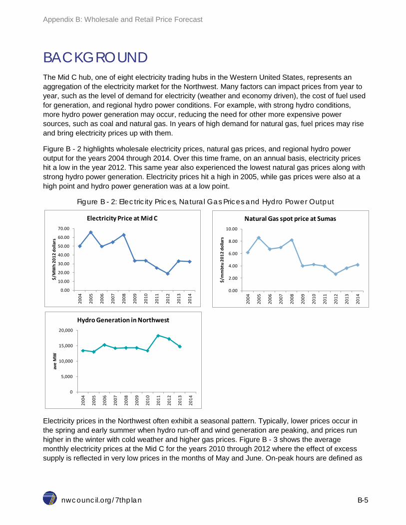
BACKGROUND The Mid C hub, one of eight electricity trading hubs in the Western United States, represents an aggregation of the electricity market for the Northwest. Many factors can impact prices from year to year, such as the level of demand for electricity (weather and economy driven), the cost of fuel used for generation, and regional hydro power conditions. For example, with strong hydro conditions, more hydro power generation may occur, reducing the need for other more expensive power sources, such as coal and natural gas. In years of high demand for natural gas, fuel prices may rise and bring electricity prices up with them.
Figure B - 2 highlights wholesale electricity prices, natural gas prices, and regional hydro power output for the years 2004 through 2014. Over this time frame, on an annual basis, electricity prices hit a low in the year 2012. This same year also experienced the lowest natural gas prices along with strong hydro power generation. Electricity prices hit a high in 2005, while gas prices were also at a high point and hydro power generation was at a low point.
Figure B - 2: Electricity Prices, Natural Gas Prices and Hydro Power Output
Electricity prices in the Northwest often exhibit a seasonal pattern. Typically, lower prices occur in the spring and early summer when hydro run-off and wind generation are peaking, and prices run higher in the winter with cold weather and higher gas prices. Figure B - 3 shows the average monthly electricity prices at the Mid C for the years 2010 through 2012 where the effect of excess supply is reflected in very low prices in the months of May and June. On-peak hours are defined as
0.00
10.00
20.00
30.00
40.00
50.00
60.00
70.00
2004
2005
2006
2007
2008
2009
2010
2011
2012
2013
2014
$/M
Wh
2012
dol
lars
Electricity Price at Mid C
0.00
2.00
4.00
6.00
8.00
10.00
2004
2005
2006
2007
2008
2009
2010
2011
2012
2013
2014
$/m
mbt
u 20
12 d
olla
rsNatural Gas spot price at Sumas
0
5,000
10,000
15,000
20,000
2004
2005
2006
2007
2008
2009
2010
2011
2012
2013
2014
ave
MW
Hydro Generation in Northwest

Appendix B: Wholesale and Retail Price Forecast
nwcouncil.org/7thplan B-6
the morning through evening hours when demand is highest, while off-peak hours include the later night time and early morning hours.
Figure B - 3: Historic Average Monthly Electricity Prices 2010-2012
In addition to hydropower, there are four other primary sources of power in the Northwest: coal, natural gas, nuclear, and wind. For the years 2004 through 2013, on average, hydropower supplied 60 percent of the region’s generation. However, hydropower’s contribution to the region can vary from year to year depending on the water conditions. Coal and natural gas fired generation in region comprised, on average, 31 percent of the region’s generation over the same time period, while winds’ share has been steadily increasing. Figure B - 4 displays the percentage of overall regional generation by resource type.
-10
0
10
20
30
40
50
1-20
10
3-20
10
5-20
10
7-20
10
9-20
10
11-2
010
1-20
11
3 -20
11
5 -20
11
7 -20
11
9 -20
11
11-2
011
1-20
12
3-20
12
5 -20
12
7-20
12
9-20
12
11-2
012
$/M
Wh
Mid C On-Peak Mid C Off-Peak

Appendix B: Wholesale and Retail Price Forecast
nwcouncil.org/7thplan B-7
Figure B - 4: Historic Regional Generation
Hydropower and wind power sources have low-variable costs which can act to keep electricity prices low. For natural gas generation, the price of fuel is a key determinant of the plant’s variable cost, and since gas plants are often the marginal generating units which set electricity prices, the price paid for natural gas fuel can directly influence wholesale electricity prices.
METHODOLOGY One of the tools the Council uses to produce the forecast is the AURORAxmp Electricity Market Model provided by EPIS. This is an economic dispatch model which means that electricity prices are based on the variable cost of the most expensive generating plant (marginal plant) or increment of load curtailment required for meeting load for each hour of the forecast period. Plant dispatch is simulated for 16 load-resource areas or zones which comprise the Western Electricity Coordinating Council (WECC). Each of the 16 zones are modeled to reflect their unique characteristics in terms of transmission constraints, load forecasts, existing generating units, scheduled project additions and retirements, fuel price forecasts, and new resource options. The dispatch model may add discretionary new resources within zones on an economic basis to maintain capacity reserve requirements or to provide energy. The demand within a zone may be served by native generation, curtailment or by imports from other zones based on economic decisions if the transmission capability exists. Transmission interconnections are characterized by transfer capacity, losses and wheeling costs. In addition to meeting demand, planning reserve margin targets are included in the model. These targets are based on the single highest hour of demand during the year.
The modeling process involves two main steps. First, a congruent set of assumptions and inputs (load, fuel prices, resource availability and costs, etc.) is established and a long-term resource optimization run is performed. This run will set any economically driven capacity additions or
0
10
20
30
40
50
60
70
80
90
100
2004 2005 2006 2007 2008 2009 2010 2011 2012 2013
Perc
enta
ge o
f Reg
iona
l Gen
erat
ion
Hydro Coal Natural Gas Nuclear Wind Other
Appendix B: Wholesale and Retail Price Forecast
nwcouncil.org/7thplan B-8
retirements over the planning horizon. Then an hourly dispatch run is completed to determine electricity prices for each zone. In addition to electricity prices, the model can also be used to evaluate other characteristics such as generation mix and carbon dioxide emission levels.
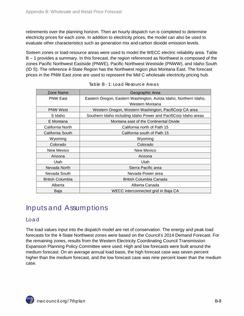
Sixteen zones or load-resource areas were used to model the WECC electric reliability area. Table B – 1 provides a summary. In this forecast, the region referenced as Northwest is composed of the zones Pacific Northwest Eastside (PNWE), Pacific Northwest Westside (PNWW), and Idaho South (ID S). The reference 4-State Region has the Northwest region plus Montana East. The forecast prices in the PNW East zone are used to represent the Mid C wholesale electricity pricing hub.
Table B - 1: Load Resource Areas
Zone Name Geographic Area PNW East Eastern Oregon, Eastern Washington, Avista Idaho, Northern Idaho,
Western Montana PNW West Western Oregon, Western Washington, PacifiCorp CA area
S Idaho Southern Idaho including Idaho Power and PacifiCorp Idaho areas E Montana Montana east of the Continental Divide
California North California north of Path 15 California South California south of Path 15
Wyoming Wyoming Colorado Colorado
New Mexico New Mexico Arizona Arizona
Utah Utah Nevada North Sierra Pacific area Nevada South Nevada Power area
British Columbia British Columbia Canada Alberta Alberta Canada
Baja WECC interconnected grid in Baja CA
Inputs and Assumptions Load
The load values input into the dispatch model are net of conservation. The energy and peak load forecasts for the 4-State Northwest zones were based on the Council’s 2014 Demand Forecast. For the remaining zones, results from the Western Electricity Coordinating Council Transmission Expansion Planning Policy Committee were used. High and low forecasts were built around the medium forecast. On an average annual load basis, the high forecast case was seven percent higher than the medium forecast, and the low forecast case was nine percent lower than the medium case.

Appendix B: Wholesale and Retail Price Forecast
nwcouncil.org/7thplan B-9
Fuel Prices
The fuel price inputs for each zone were based on updated natural gas and coal forecasts from the Council’s fuel model. This is a fundamentals gas model which estimates prices at western gas hubs. High and low fuel price forecasts were also developed around the medium forecast. The high price case was 50 percent higher than the medium case on an average annual basis, while the low price case was 43 percent lower than the medium case. The high and low bands around the gas price assume there is more room for prices to run higher; it’s generally accepted that there is a floor to prices at which there would be a cut back on drilling rigs, resulting in a more firm lower price band.
Resources
A comprehensive update of the resource base for the dispatch model was completed. The data sources included the 2012 EIA-860 Annual Electric Generation Data Report, the Council’s Northwest Generating Resource database, and the Council’s resource tracking worksheets. As in previous Council forecasts, projects under construction and resources in advanced development are considered to be committed and completed as scheduled.
Announced retirements are assumed to occur when scheduled. Several coal plants, including Boardman, Centralia and North Valmy in the Northwest are assumed to close by 2026. Table B - 2 contains a list of a few key coal unit retirements with dates and capacity.
Table B - 2: Retiring Coal Units
Unit Zone Fuel Retirement Year
Installed Capacity MW
Corette 1 MT E Coal 2015 154 Boardman 1 PNW E Coal 2020 585 Centralia 1 PNW W Coal 2020 670 Centralia 2 PNW W Coal 2025 670
North Valmy Nevada N Coal 2025 522
Pacific Northwest Hydro Modeling
To simulate Pacific Northwest hydroelectric generation in AURORAxmp, annual average capacity factors and monthly shape factors were calculated for the three load-resource areas: PNW West, PNW East, and S Idaho based on historic data. The data set was comprised of 80 years of stream flow data from the years of 1929 through 2008.
Renewable Portfolio Standards
Washington, Oregon, and Montana have all passed renewable portfolio standards (RPS) in which a certain percentage of qualifying utilities’ electricity sales are required to be produced from renewable resources. While each state has a unique standard with varying factors (e.g. eligible resources, technology minimums, banking provisions), they all have the same overall objective to encourage the development and procurement of renewable resources in the Pacific Northwest over the next decade or so.

Appendix B: Wholesale and Retail Price Forecast
nwcouncil.org/7thplan B-10
Table B - 3: RPS in the Northwest
Montana Oregon Washington Standard 10% in 2010
15% in 2015*
5% in 2011
15% in 2015
20% in 2020
25% in 2025*
3% in 2012
9% in 2016
15% in 2020*
* and each year thereafter
So far, the region has been on track, and even ahead, in meeting most of the interim targets set by the renewable portfolio standards. The significant development of wind power in the late 2000’s and early 2010’s set the region up to be in good shape until around 2020, when further renewable resource acquisition will be needed to meet the final goals.
Carbon Dioxide Regulatory Policy Carbon dioxide emission pricing policies can impact electricity prices by attaching an emission cost to fossil fuel generation, and by influencing decisions to incorporate more non-emitting resources into the generation mix. In the Western US, California implemented a Cap and Trade program for carbon in 2013 and the British Columbia Parliament begin imposing a carbon tax in 2008.
A carbon dioxide price curve for the California Cap and Trade program was implemented in the model as a cost in terms of $/ton of carbon dioxide emitted for generation residing in the two California zones. In addition, a hurdle rate expressed in $/MWh was applied to energy that was imported to California based on emitting intensity. The initial cost point for the carbon dioxide cost curve was based on the allowance price from the California Air Resources Board Quarterly Auction, and was increased each year at an annual rate of five percent as suggested by the Resources Board.
British Columbia instituted a carbon tax in July of 2008 at $10/metric ton carbon dioxide, and increased the tax five dollars per year until reaching $30/metric ton in 2012. For this forecasting cycle, it is expected that the tax would remain at the $30 level for the forecast horizon. This price for carbon was attached to carbon dioxide emitting resources that reside within British Columbia.
The carbon dioxide price curves which were used in the model are shown in Figure B-5.

Appendix B: Wholesale and Retail Price Forecast
nwcouncil.org/7thplan B-11
Figure B - 5: Carbon Dioxide Emission Prices as Modeled
RESULTS Five primary forecast cases were defined and run through the AURORAxmp pricing model:
1. Medium 2. High Demand 3. Low Demand 4. High Fuel 5. Low Fuel
For each of the cases, the same RPS and Greenhouse Gas policies were assumed, as well as average hydro conditions. The Medium case used the medium forecasts for electricity load and natural gas, and coal fuel prices. For the High Demand case, load was adjusted up by approximately seven percent while keeping the medium fuel price forecast. In the Low Demand case, load was adjusted down by approximately nine percent from the medium case. In the High Fuel case, the medium demand forecast was used, but fuel prices were increased by roughly 50 percent. In the Low Fuel case, the fuel price forecast was dropped by approximately 43 percent. As seen in Figure B - 1, the High Fuel and Low Fuel cases provided the upper and lower bounds for the wholesale electricity price forecast range.
In addition to electricity prices, other outputs from the forecast model include generation output by type, and carbon dioxide emission levels.
0
5
10
15
20
25
30
35
2016
2017
2018
2019
2020
2021
2022
2023
2024
2025
2026
2027
2028
2029
2030
2031
2032
2033
2034
2035
$/to
n CO
2 20
12 d
olla
rs
CA Carbon Cap and Trade British Columbia Carbon Tax

Appendix B: Wholesale and Retail Price Forecast
nwcouncil.org/7thplan B-12
Medium Case Under medium forecast conditions (load, fuel, hydro) and current greenhouse gas emission policies, the price for electricity at the Mid C in real 2012 dollars is expected to increase from year to year at an average rate of around three percent. Prices generally follow annual increases in fuel price.
Annual and Monthly Prices
Figure B - 6 displays the wholesale electricity price forecast broken out into high and low load hours on an annual and monthly basis. Heavy load hours are defined as the morning through evening hours when demand is highest, while the light load hours include the later night time and early morning hours. The seasonal effect of hydro and wind can be seen in the monthly prices. Typically prices are lowest in May and June when demand is modest and hydro power generation is peaking, and highest in December and January when demand is highest under cold weather.
Figure B - 6: Wholesale Electricity Price Forecast at Mid C
Generation Mix
Figure B - 7 shows the range of percentages that each resource type produces in the forecast model. Because average hydro conditions are assumed for each year, the range of generation from hydro power does not vary much from year to year in the forecast and is consistent with historic results. The percentage of generation from coal is seen to decline over time as coal plant retirements occur, while natural gas and wind generation increases.
0
10
20
30
40
50
60
2016
_01
2017
_02
2018
_03
2019
_04
2020
_05
2021
_06
2022
_07
2023
_08
2024
_09
2025
_10
2026
_11
2027
_12
2029
_01
2030
_02
2031
_03
2032
_04
2033
_05
2034
_06
2035
_07
$/M
Wh
2012
dol
lars
Monthly
Light Load Hours Heavy Load Hours
0
10
20
30
40
50
60
2016 2018 2020 2022 2024 2026 2028 2030 2032 2034
$/M
Wh
2012
dol
lars
Annual
Light Load Hours Heavy Load Hours

Appendix B: Wholesale and Retail Price Forecast
nwcouncil.org/7thplan B-13
Figure B - 7: Forecast Regional Generation
Carbon Dioxide Emissions
In the Medium Forecast case, carbon dioxide emissions from regional power generation decline over time as the coal units in Boardman and Centralia are retired. On an intensity basis of pounds CO2 per MWh of electricity produced, the forecast shows the region declining from 0.51 pounds per MWh in 2016 to 0.41 pounds per MWh by 2031. This includes all generating resources. On an intensity basis, the Northwest emits at a low rate relative to other regions due to the dominance of non-emitting hydro and wind power. Figure B - 8 displays carbon dioxide emissions from power generation from the region on an annual basis. The effect of the coal unit retirements in 2020 and 2025 can clearly be seen in the chart.
0
10
20
30
40
50
60
70
Hydro Natural Gas Coal Wind Nuclear
Perc
enta
ge %

Appendix B: Wholesale and Retail Price Forecast
nwcouncil.org/7thplan B-14
Figure B - 8: Forecast Regional Carbon Dioxide Emissions from Power Generation
Natural Gas Price and Electricity Price
As mentioned earlier, the price of natural gas used as fuel for generating electricity has a strong influence on wholesale electricity price, and this relationship is expected to continue in the future. Existing hydro and wind power provide low-variable cost (no on-going fuel related expenses) power to the region. Coal and especially natural gas fired plants (more easily dispatched) have larger variable costs and are therefore often the marginal generating unit which set wholesale electricity prices. A major variable cost component for gas plants is fuel consumption; therefore the price for the fuel that is consumed becomes highly influential. Moving forward, as the regional coal units retire through time, the Northwest may be even more influenced by the price of natural gas.
Figure B - 10 displays the relationship between the wholesale electricity price and natural gas price. Annual natural gas prices are shown on the x-axis, and corresponding annual electricity prices on the y-axis. The graph shows both historic and forecast data points from the Mid C and the Sumas gas pricing hub. The result is a linear relationship between gas and electricity, which suggests that it would be wise to spend time examining expectations around future natural gas prices in order to see where electricity prices may be headed.
0
10
20
30
40
50
60
70
2016
2017
2018
2019
2020
2021
2022
2023
2024
2025
2026
2027
2028
2029
2030
2031
2032
2033
2034
2035
mm
Tons
CO
2
Natural Gas Coal (including Colstrip MT) Other

Appendix B: Wholesale and Retail Price Forecast
nwcouncil.org/7thplan B-15
Figure B - 9: Relationship of Electricity Price to Natural Gas Price
0
10
20
30
40
50
60
70
0 2 4 6 8 10
Elec
tric
ity P
rice
$/M
Wh
(201
2$)
Natural Gas Price $/mmbtu (2012$)
Historic Electricity Mid C Price
Medium Forecast Electricity Price Mid C
Linear Fit Electric Price
Appendix B: Wholesale and Retail Price Forecast
nwcouncil.org/7thplan B-16
FORECAST OF RETAIL ELECTRICITY PRICES Introduction This section presents the methodology used to estimate the average revenue requirement per megawatt-hour and average residential bills for the least risk resource plan under various scenarios. Revenue requirements are the amount of revenue a utility needs to collect to pay for all generation, transmission, distribution, conservation program and non-program costs, and for investor-owned utilities, the allowed return on capital investments. The average revenue requirement per megawatt-hour is calculated by dividing the total revenue requirement by the megawatt hours of sales to customers. Average residential bills are calculated by dividing the residential sector’s share of total revenue requirement by number of residential customers. The scenarios are described in Chapter 3 (“Resource Strategy”). These average revenue requirements and bills reflect the impact of conservation investment, CO2 tax revenues and the cost of other resources developed in the least cost resource strategy for each scenario.
It should be emphasized that these average revenue requirements per megawatt-hour are not intended to represent the Council’s estimates of retail electricity rates. The methodology used to derive average revenue requirements per megawatt-hour is a gross simplification of the detailed calculations and regulatory approval process that is used to establish utility retail rates. Actual rate setting procedures and calculations will vary across utilities, class of customers and regulatory jurisdictions. The average revenue requirements per megawatt-hour calculations presented here are averaged across all customer classes, so relative changes among classes are not reflected. The results should, however, be valid for comparison across scenarios.
Methodology for Estimating Average Revenue Requirements To estimate the average revenue requirement per megawatt-hour, the total regional revenue requirement in dollars is divided by the total regional retail sales of electricity. To calculate the total regional revenue requirement, the fixed cost of the existing power system that must be paid for was added to the average development and operational cost of the future power system across all 800 futures estimated by the RPM for each scenario. The fixed cost of the existing power system is assumed to remain unchanged at 2015 levels in real terms over the 20 year period covered by the Seventh Plan. This implicitly assumes that the capital additions to necessary to maintain the existing power system are exactly equal to the depreciation of the cost of the existing power system. The future system costs consist of the capital cost of the new resources and the non-capital cost of the existing and future power system. The future system cost is the cost calculated in the Regional Portfolio Model (RPM). The consumer’s contribution to conservation measures is netted from the total system cost calculated in the RPM. The average revenue requirements per megawatt-hour and average residential monthly electric bills are an average of the revenue requirements and bills across all 800 possible futures.

Appendix B: Wholesale and Retail Price Forecast
nwcouncil.org/7thplan B-17
Estimating Existing Power System Cost:
The total regional revenue from electricity sales for the Northwest power system in 2013, as reported by EIA-Form 861, was $12.8 billion. The Council estimates that about 85 percent of that requirement, about $10.8 billion per year, is the fixed costs of the existing system.
Estimating Future Power System Cost:
The cost of the future power system calculated in the Regional Portfolio Model (RPM) consists of levelized costs of conservation resources and capital and non-capital costs of other new resources as well as the variable cost of existing system. However, general practice among utilities for at least the last decade has been to “expense” their conservation expenditures, that is, to recover them in rates immediately rather than capitalize the expenditures and recover them (and accumulated interest) over the life of the conservation measures. To reflect this practice in the Council’s estimates of average revenue requirement per megawatt-hour, estimated conservation costs “as incurred” were substituted for the levelized conservation costs1 used in the RPM. Based on recent history, $420 million per year of conservation expenses were assumed to be included in the 2015 revenue requirement; so that conservation development expenses in the future would only increase revenue requirements to the extent they are higher than $420 million per year.
To estimate these “as incurred” costs, Council staff converted the levelized costs of the conservation developed by the RPM into a single payment to be made at the time of the conservation measures’ installation. This payment covers the full installation cost of the measures, and their administration cost over their lifetime, expressed as 2012 dollars per average megawatt of yearly savings. This approach assures the calculation method is consistent with the method used to develop the conservation supply curve costs used by the RPM. The average total cost per average megawatt of all conservation developed by the RPM over the 20 years covered by the Seventh Plan was estimated at $6.25 million in 2012 dollars.
Since consumers traditionally share in the cost of conservation, not all of the $6.25 per average megawatt cost must be recovered in utility revenue requirements. Based on historical experience in the region, the Council assumed that approximately 65 percent of the cost of conservation is paid by the utility system and, therefore, must be recovered in revenue requirements. Two further adjustments were made to reflect the fact that conservation savings defer investments in distribution and transmission and compensate for the 10 percent Regional Power Act Conservation Credit which was included in the original $6.25 million per average megawatt costs. The result of these adjustments results in an average utility cost of $3.01 million per average megawatt of conservation savings.
1 The conservation premium used to select the level of conservation acquisition does not change the cost of conservation resources and the levelized cost of conservation and the cash-flow of expensed conservation do not differ greatly if conservation acquisition levels are increasing smoothly and do not have significant jumps from one year to next.
Appendix B: Wholesale and Retail Price Forecast
nwcouncil.org/7thplan B-18
Cost of CO2 Tax Revenues
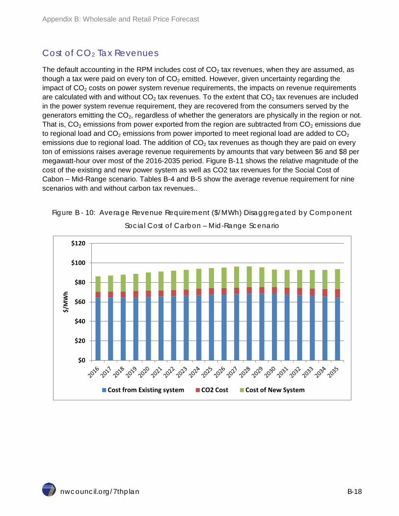
The default accounting in the RPM includes cost of CO2 tax revenues, when they are assumed, as though a tax were paid on every ton of CO2 emitted. However, given uncertainty regarding the impact of CO2 costs on power system revenue requirements, the impacts on revenue requirements are calculated with and without CO2 tax revenues. To the extent that CO2 tax revenues are included in the power system revenue requirement, they are recovered from the consumers served by the generators emitting the CO2, regardless of whether the generators are physically in the region or not. That is, CO2 emissions from power exported from the region are subtracted from CO2 emissions due to regional load and CO2 emissions from power imported to meet regional load are added to CO2 emissions due to regional load. The addition of CO2 tax revenues as though they are paid on every ton of emissions raises average revenue requirements by amounts that vary between $6 and $8 per megawatt-hour over most of the 2016-2035 period. Figure B-11 shows the relative magnitude of the cost of the existing and new power system as well as CO2 tax revenues for the Social Cost of Cabon – Mid-Range scenario. Tables B-4 and B-5 show the average revenue requirement for nine scenarios with and without carbon tax revenues..
Figure B - 10: Average Revenue Requirement ($/MWh) Disaggregated by Component
Social Cost of Carbon – Mid-Range Scenario
$0
$20
$40
$60
$80
$100
$120
$/M
Wh
Cost from Existing system CO2 Cost Cost of New System

Appendix B: Wholesale and Retail Price Forecast
nwcouncil.org/7thplan B-19
Calculated Average Revenue Requirements
The methodology described above results in the annual and levelized revenue requirements per megawatt-hour for the period 2016 through 2035. The results in Tables B-4 and B-5 illustrate ten of the scenarios described in Chapter 3. As an illustrative example, under the Carbon Cost Risk scenario the average revenue requirement increases from $82 per megawatt-hour in 2016 to $80-$99 per megawatt-hour by 2035 if CO2 taxes are not borne by consumers and nearly $82-$99 per megawatt-hour in 2035 if they are.
Table B - 4: Annual Average Revenue Requirement per mega-watt hours in $2012/MWh - Excluding CO2 Tax Revenues
Existing Policy
SCC - Mid-Range
Max. CO2 Reduction - Exist. Tech.
Retire Coal
Retire Coal w/
SCC_Mid Range
Retire Coal w/SCC_MidRange & No New Gas
Increased Market Reliance
No Demand Response
Regional RPS at 35%
Lower Conservation
2016 81 81 82 81 81 81 81 81 81 80 2017 82 82 83 82 81 82 81 82 82 80 2018 83 82 84 83 82 82 82 83 83 80 2019 83 83 85 83 83 83 82 84 83 81 2020 84 84 86 84 83 84 83 85 85 81 2021 85 85 87 85 84 85 84 86 89 81 2022 86 85 89 86 85 86 85 87 92 82 2023 87 86 91 88 88 89 85 88 94 82 2024 87 86 92 89 89 91 86 88 96 82 2025 88 86 93 90 89 95 86 89 98 82 2026 88 87 94 90 88 95 86 89 101 82 2027 88 87 95 91 89 96 86 89 106 83 2028 89 87 96 92 89 96 87 90 106 83 2029 86 85 96 90 87 94 84 88 104 83 2030 84 83 94 88 85 92 83 86 101 83 2031 84 83 93 87 85 91 82 85 100 83 2032 83 82 93 87 84 91 81 84 98 82 2033 83 82 94 89 87 99 81 84 97 86 2034 82 82 94 89 87 100 81 84 96 87 2035 82 82 95 88 87 99 80 83 95 86
Levelized $84.71 $84.01 $89.91 $86.6 $85.31 $89.35 $83.35 $85.63 $92.97 $82.11 Annual Rate of growth 0.1% 0.1% 0.8% 0.4% 0.4% 1.1% -0.1% 0.1% 0.8% 0.4%

Appendix B: Wholesale and Retail Price Forecast
nwcouncil.org/7thplan B-20
Table B - 5: Annual Average Revenue Requirement per mega-watt hours in $2012/MWh - Including CO2 Cost
Existing Policy
SCC - Mid-Range
Max. CO2 Reduction - Exist. Tech.
Retire Coal
Retire Coal w/
SCC_Mid Range
Retire Coal w/SCC_Mid
Range & No New Gas
Increased Market Reliance
No Demand Response
Regional RPS at 35%
Lower Conservation
2016 81 87 82 81 86 87 81 81 81 80 2017 82 88 83 82 87 88 81 82 82 80 2018 83 89 84 83 88 89 82 83 83 80 2019 83 90 85 83 90 90 82 84 83 81 2020 84 91 86 84 91 92 83 85 85 81 2021 85 92 87 85 92 92 84 86 89 81 2022 86 93 89 86 93 93 85 87 92 82 2023 87 93 91 88 95 97 85 88 94 82 2024 87 94 92 89 96 98 86 88 96 82 2025 88 94 93 90 97 102 86 89 98 82 2026 88 95 94 90 96 101 86 89 101 82 2027 88 95 95 91 96 101 86 89 106 83 2028 89 95 96 92 96 101 87 90 106 83 2029 86 93 96 90 95 99 84 88 104 83 2030 84 91 94 88 93 98 83 86 101 83 2031 84 91 93 87 92 97 82 85 100 83 2032 83 91 93 87 92 97 81 84 98 82 2033 83 91 94 89 95 104 81 84 97 86 2034 82 91 94 89 95 105 81 84 96 87 2035 82 90 95 88 94 102 80 83 95 86
Levelized $84.71 $91.5 $89.91 $86.6 $92.49 $95.61 $83.35 $85.63 $92.97 $82.11 Annual Rate of growth 0.1% 0.2% 0.8% 0.4% 0.5% 0.8% -0.1% 0.1% 0.8% 0.4%

Appendix B: Wholesale and Retail Price Forecast
nwcouncil.org/7thplan B-21
Comparison of annual electric revenues collected in the region, for the past 24 years, with the forecasted future revenue requirement is presented in the Figure B-12. To make the comparison across time appropriate all costs were first converted to 2012 dollars and then indexed so that 2012 has an index value of 100. Between 1990 and 2012, Northwest power systems revenue requirement increased by approximately 27 index points. In the future period, the revenue requirement is expected to increase from an index of 100 points to 116 to 140 points, depending on how CO2 tax revenues are incorporated into the revenue requirement. The future increase in average revenue requirement per megawatt-hour is anticipated to be less than historic experience under the Coal retirement scenario with or without consideration of CO2 tax revenues.
Figure B - 11: Comparison of Historic Revenue Collected and Future Revenue Requirement Indexed to 2012
Calculated Monthly Bills
Representative residential average monthly bills were estimated using the total revenue requirements calculated earlier. The residential sector’s share of those annual revenue requirements was estimated at 47 percent based on the most recent data. To compute average monthly residential bills 47 percent of future revenue requirements were divided by the projected number of households in future years and then again by 12 to arrive at monthly bills per household. The results of those calculations are shown in Tables B-6 and B-7.
0
20
40
60
80
100
120
140
160
1990
1992
1994
1996
1998
2000
2002
2004
2006
2008
2010
2012
2014
2016
2018
2020
2022
2024
2026
2028
2030
2032
2034
Retire Coal
Retire Coal w/SCC_MidRange
Existing Policies, No Carbon Risk

Appendix B: Wholesale and Retail Price Forecast
nwcouncil.org/7thplan B-22
Table B - 6: Average Residential Bills for Least Cost Resource Strategy by Scenario – CO2 Tax Revenues Excluded
(Bills are expressed in 2012$/month/household)
Existing Policy
SCC - Mid-Range
Max. CO2 Reduction - Exist. Tech.
Retire Coal
Retire Coal w/SCC_Mid
Range
Retire Coal w/SCC_
Mid Range & No New Gas
Increased Market Reliance
No Demand Response
Regional RPS at 35%
Lower Conservation
2016 74 74 75 92 74 74 74 74 74 73 2017 73 73 74 90 72 73 73 73 73 72 2018 72 72 73 90 72 72 72 73 72 71 2019 72 71 73 89 71 72 71 72 72 71 2020 72 71 73 89 71 71 71 72 72 70 2021 71 70 72 88 70 70 70 71 75 70 2022 70 70 72 87 70 70 70 71 76 69 2023 70 69 72 88 71 71 69 70 76 69 2024 69 68 72 87 70 71 68 69 76 69 2025 68 67 72 87 69 73 68 69 77 68 2026 67 66 71 86 67 72 67 68 78 68 2027 67 65 71 85 67 71 66 67 80 67 2028 66 64 70 84 66 70 65 66 80 67 2029 63 62 69 82 64 68 63 64 77 67 2030 61 60 68 80 62 66 61 62 75 67 2031 61 59 67 79 61 65 60 61 73 66 2032 60 59 67 79 61 65 60 60 73 66 2033 60 59 68 80 63 70 60 61 72 69 2034 60 59 68 81 63 71 60 61 71 70 2035 60 59 69 80 63 70 59 60 71 69
Levelized $67.90 $67.03 $71.33 $86.06 $68.24 $70.64 $67.45 $68.28 $74.66 $69.26 Annual Rate of growth -1.1% -1.2% -0.4% -0.7% -0.8% -0.3% -1.2% -1.1% -0.2% -0.3%
Appendix B: Wholesale and Retail Price Forecast
nwcouncil.org/7thplan B-23
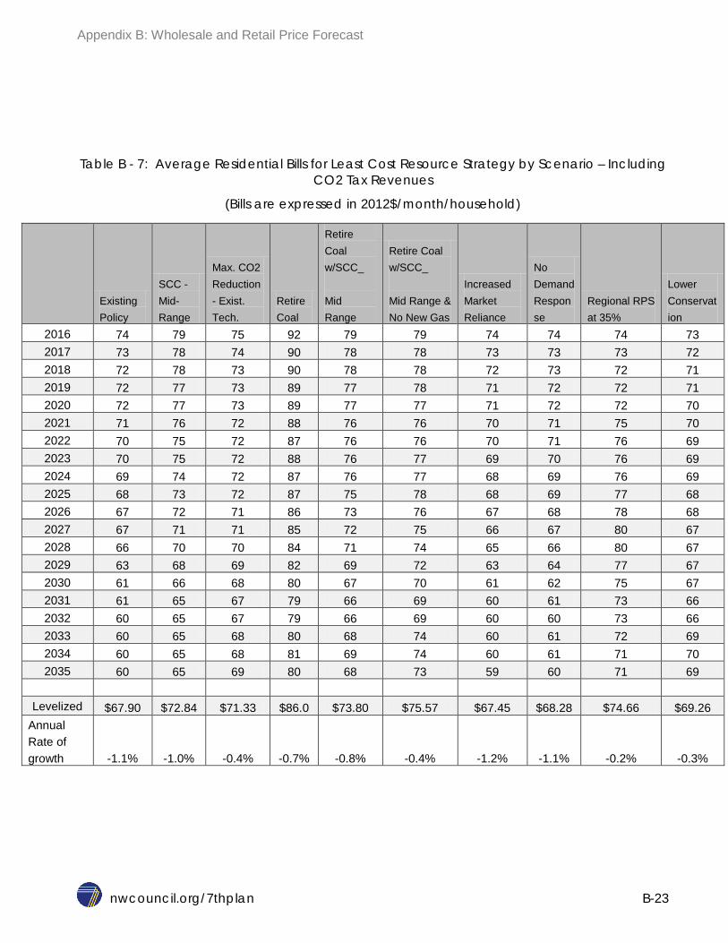
Table B - 7: Average Residential Bills for Least Cost Resource Strategy by Scenario – Including CO2 Tax Revenues
(Bills are expressed in 2012$/month/household)
Existing Policy
SCC - Mid-Range
Max. CO2 Reduction - Exist. Tech.
Retire Coal
Retire Coal w/SCC_
Mid Range
Retire Coal w/SCC_
Mid Range & No New Gas
Increased Market Reliance
No Demand Response
Regional RPS at 35%
Lower Conservation
2016 74 79 75 92 79 79 74 74 74 73 2017 73 78 74 90 78 78 73 73 73 72 2018 72 78 73 90 78 78 72 73 72 71 2019 72 77 73 89 77 78 71 72 72 71 2020 72 77 73 89 77 77 71 72 72 70 2021 71 76 72 88 76 76 70 71 75 70 2022 70 75 72 87 76 76 70 71 76 69 2023 70 75 72 88 76 77 69 70 76 69 2024 69 74 72 87 76 77 68 69 76 69 2025 68 73 72 87 75 78 68 69 77 68 2026 67 72 71 86 73 76 67 68 78 68 2027 67 71 71 85 72 75 66 67 80 67 2028 66 70 70 84 71 74 65 66 80 67 2029 63 68 69 82 69 72 63 64 77 67 2030 61 66 68 80 67 70 61 62 75 67 2031 61 65 67 79 66 69 60 61 73 66 2032 60 65 67 79 66 69 60 60 73 66 2033 60 65 68 80 68 74 60 61 72 69 2034 60 65 68 81 69 74 60 61 71 70 2035 60 65 69 80 68 73 59 60 71 69
Levelized $67.90 $72.84 $71.33 $86.0 $73.80 $75.57 $67.45 $68.28 $74.66 $69.26
Annual Rate of growth -1.1% -1.0% -0.4% -0.7% -0.8% -0.4% -1.2% -1.1% -0.2% -0.3%
Seventh Northwest Conservation and Electric Power Plan
nwcouncil.org/7thplan C-1
APPENDIX C: FUEL PRICE FORECAST
Contents Introduction ....................................................................................................................................... 3 Dealing with Uncertainty and Volatility ............................................................................................... 4 Natural Gas ....................................................................................................................................... 5
Background ................................................................................................................................ 5 Price Forecasts .............................................................................................................................. 7
U.S. Natural Gas Commodity Prices .......................................................................................... 7 Northwest Natural Gas Supplies and Price ............................................................................... 10
Oil ................................................................................................................................................... 13 Background .............................................................................................................................. 13 Oil Price Forecast Range ......................................................................................................... 13
Coal ................................................................................................................................................ 16 Coal Commodity Prices ............................................................................................................... 16 Coal Price Forecast ..................................................................................................................... 17
Methodology .................................................................................................................................... 18 From Source to Burnertip ............................................................................................................. 18
List of Figures and Tables
Figure C - 1: Fluctuations in commodity prices Indexed to 2005 ........................................................ 4 Figure C - 2: Historical Wellhead Natural Gas Price ($2012/mmBtu) ................................................ 6 Figure C - 3: Historical Natural Gas Prices 2012$/mmBtu and Consumption (Trillion Cubic Ft) ........ 7 Figure C - 4: U.S. Wellhead Natural Gas Price Forecast Range 2012 $/mmBTU ............................. 9 Figure C - 5: Pacific Northwest Natural Gas Infrastructure and Capacities (Millions of Dekatherms) 11 Figure C - 6: Historical Comparison of Crude Oil and Wellhead Natural Gas Prices ....................... 13 Figure C - 7: World Oil Prices: History and Forecast (2012$/Barrel) ............................................... 14 Figure C - 8: Total U.S. Petroleum Use per Millions of 2005 Dollar of Gross Domestic Product ...... 15 Figure C - 9: Coal Price Trends from Major Supply Areas ($/Short tons) ........................................ 17 Figure C - 10: Range of Powder River Basin Coal Price Forecasts (2012$/mmBtu) ....................... 17 Table C - 1: Relationship between Wellhead, Henry Hub and Burner-tip prices .............................. 18 Table C - 2: Monthly Shape of Prices .............................................................................................. 19

Appendix C: Fuel Price Forecast
nwcouncil.org/7thplan C-2
Please note that a companion workbook will be available with additional detail on forecasted prices on the Council’s website at http://www.nwcouncil.org/energy/powerplan/7/technical
Throughout this write-up fuel forecast is presented in form of a low and high range. This is done to reinforce the fact that future is uncertain. Council’s planning process does not use a single deterministic future to drive the analysis. The stochastic variation introduced in the Regional Portfolio Model tests a wide range of future uncertainties in load, fuel prices etc.
Appendix C: Fuel Price Forecast
nwcouncil.org/7thplan C-3
INTRODUCTION This appendix summarizes fuel price forecasts for natural gas, oil and coal. Since the millennium, the trend for fuel prices has been one of uncertainty and volatility. The price of crude oil was $25 per barrel in January of 2000. In July 2008 it averaged $127/barrel, even approaching $150/barrel some days, today it is less than $45/barrel. Natural gas prices at the wellhead averaged $2.37 per million Btu in January 2000. In June 2008, the average wellhead price of natural gas averaged $12.60/mmBtu, as of April 13, 2015 Henry Hub price was $2.60/mmBtu. The reduction in oil and natural gas prices were the result of large supply availability and low demand. Demand was low due to slow global recovery and supply was high due to greater use of hydraulic fracturing of source rock.
The Seventh Power Plan natural gas price forecast is significantly lower than the Sixth Power Plan’s forecast. However, price uncertainty remains, not only with fuels, but also with other commodities such as metals, concrete, plastics, and other construction materials have all experienced fluctuation in prices. Various factors have contributed to higher or lower commodity prices in general, and to fuel prices in particular, including: fluctuations in world economic growth, fluctuating value of the dollar, response of conventional energy supplies to higher prices, continuing conflicts in the Middle East and Eastern Europe, uncertainty about the direction of climate change policy, and changing commodity market dynamics.
The relative contribution of these factors to fluctuation in prices is uncertain, as is the direction of change for many of them. Conventional sources of oil and natural gas in North America are expected to be difficult to expand significantly. Growth in supplies, therefore, will increasingly depend on the development of unconventional sources and liquefied natural gas (LNG) exports. With the recent fluctuations in natural gas prices and technological improvements in drilling, nonconventional supplies of natural gas have expanded rapidly. United States is going from being an importer of LNG to a significant exporter of LNG.
High prices can bring about changes on the demand side of the market. High prices encourage curtailing energy use and also create incentives to invest in energy-efficient technologies. Such responses to high prices set in motion the forces to reduce prices. Over time, these cycles are likely to reach higher high points and higher low points, forming a series of upward-stepping cycles. Investments in new supplies and energy efficiency also tend to follow these cycles. Expectations that prices will fall from high points in the cycle make consistent investments in supply and energy efficiency less robust.
Accurately forecasting future fuel prices is an impossible task. Even long-term forecasts tend to assume that current conditions will, to a large extent, continue. During periods of high fuel prices, forecasts tend to increase, and during periods of low prices, they tend to decrease. The Council’s practice has been to recognize the inherent uncertainty and build power plants that minimize the risk from price forecasts that turn out to be wrong. Figure C - 1 shows the monthly fluctuations in commodity prices, according to International Monetary Fund. Planning deterministically under the range of fluctuations will lead to errors.

Appendix C: Fuel Price Forecast
nwcouncil.org/7thplan C-4
Figure C - 1: Fluctuations in commodity prices Indexed to 2005
DEALING WITH UNCERTAINTY AND VOLATILITY In spite of their uncertainty, fuel prices are an important consideration for electricity planning. Fuel prices affect both the demand for, and the cost of electricity. As an important determinant of electricity cost, fuel prices also affect the cost-effective amount of conservation through the avoided cost of alternative generation resources. The uncertainty and volatility of fuel prices create risks for the Northwest power system. These risks and others are addressed in the Council’s electricity planning process in the Regional Portfolio Model.
The range of trend forecasts discussed in this section represents only one aspect of fuel price uncertainty addressed in the Council’s power plan. The low to high trend forecasts of fuel prices are meant to reflect current analysis and views on the likely range of future prices, but the plan’s analysis also considers variations expected to occur around those trends. In the Power Plan this additional volatility was applied to natural gas prices. This was because oil prices are insignificant as either a demand alternative to electricity or a generation fuel. Coal prices are a significant determinant of electricity costs because of existing coal-fired generation, and coal is also a potential future source of energy. However, coal prices had not experienced the same level of uncertainty and
0
50
100
150
200
250
300 19
92M
1 19
92M
9 19
93M
5 19
94M
1 19
94M
9 19
95M
5 19
96M
1 19
96M
9 19
97M
5 19
98M
1 19
98M
9 19
99M
5 20
00M
1 20
00M
9 20
01M
5 20
02M
1 20
02M
9 20
03M
5 20
04M
1 20
04M
9 20
05M
5 20
06M
1 20
06M
9 20
07M
5 20
08M
1 20
08M
9 20
09M
5 20
10M
1 20
10M
9 20
11M
5 20
12M
1 20
12M
9 20
13M
5 20
14M
1 20
14M
9
All Commodities Prices Non-Fuel Price Food and Baverage Prices
Industrial Input Price Metal Prices Fuel Energy Prices

Appendix C: Fuel Price Forecast
nwcouncil.org/7thplan C-5
volatility as oil and natural gas prices, and were therefore not considered to be a major source of risk and uncertainty.
The plan reflects three distinct types of uncertainty in natural gas prices: (1) uncertainty about long-term trends, (2) price excursions due to disequilibrium of supply and demand that may occur over a number of years, and (3) short-term and seasonal volatility due to factors such as temperatures, storms, or natural gas storage levels. The fuel price forecasts include only the first uncertainty. Shorter-term variations are addressed in the Council’s Regional Portfolio Model analysis.
There are additional uncertainties to the cost of fuel from the effects of climate policies, such as CO2 costs from taxes or a cap and trade structure. These additional costs are explicitly treated in the Council’s portfolio model and affect the cost of using various fuels, but are not a part of the commodity prices discussed in this appendix.
NATURAL GAS Background
The Council’s forecast of natural gas prices starts with a national level commodity price, the average natural gas wellhead price in the lower-48 states. The past behavior of these prices gives perspective for the forecasts. Figure C - 2 shows wellhead natural gas prices (in constant 2012 dollars per million Btu) from 1980 through 2014. Following deregulation of natural gas markets in the late 1980s, prices fell to nearly $2.30/mmBtu and remained near that level for all of the 1990s. After 2000, prices began to increase rapidly and became highly volatile. By 2008 the wellhead price of natural gas averaged $8/mmBtu, nearly four times the levels of the 1990s. In some months since 2000, prices have reached over $10/mmBtu as they responded to the effects of hurricanes, storage levels, oil prices, and other market effects. With this historical context, it is difficult to predict future natural gas prices with any certainty. Post 2008 we see a period of declining base prices. By 2013 and 2014 natural gas prices have been in the $3.50 to $2.50/mmBtu range. In 2015, Henry Hub natural gas prices average to $2.64 per mmBtu.
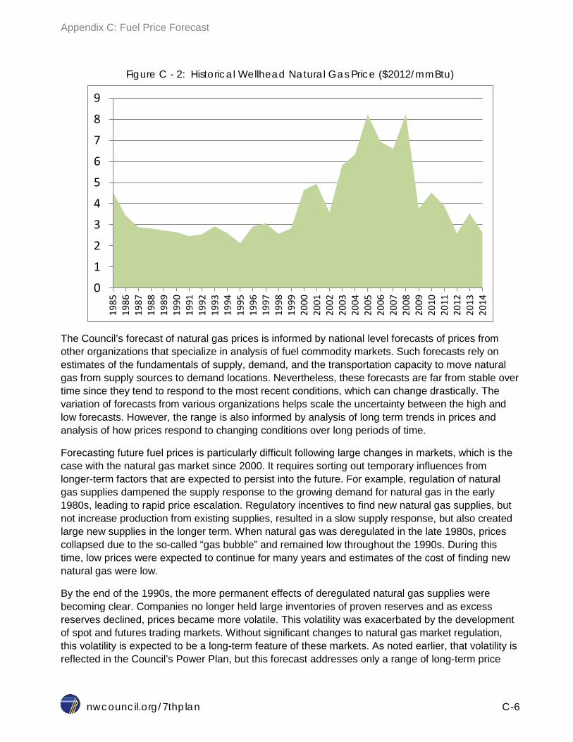
Appendix C: Fuel Price Forecast
nwcouncil.org/7thplan C-6
Figure C - 2: Historical Wellhead Natural Gas Price ($2012/mmBtu)
The Council’s forecast of natural gas prices is informed by national level forecasts of prices from other organizations that specialize in analysis of fuel commodity markets. Such forecasts rely on estimates of the fundamentals of supply, demand, and the transportation capacity to move natural gas from supply sources to demand locations. Nevertheless, these forecasts are far from stable over time since they tend to respond to the most recent conditions, which can change drastically. The variation of forecasts from various organizations helps scale the uncertainty between the high and low forecasts. However, the range is also informed by analysis of long term trends in prices and analysis of how prices respond to changing conditions over long periods of time.
Forecasting future fuel prices is particularly difficult following large changes in markets, which is the case with the natural gas market since 2000. It requires sorting out temporary influences from longer-term factors that are expected to persist into the future. For example, regulation of natural gas supplies dampened the supply response to the growing demand for natural gas in the early 1980s, leading to rapid price escalation. Regulatory incentives to find new natural gas supplies, but not increase production from existing supplies, resulted in a slow supply response, but also created large new supplies in the longer term. When natural gas was deregulated in the late 1980s, prices collapsed due to the so-called “gas bubble” and remained low throughout the 1990s. During this time, low prices were expected to continue for many years and estimates of the cost of finding new natural gas were low.
By the end of the 1990s, the more permanent effects of deregulated natural gas supplies were becoming clear. Companies no longer held large inventories of proven reserves and as excess reserves declined, prices became more volatile. This volatility was exacerbated by the development of spot and futures trading markets. Without significant changes to natural gas market regulation, this volatility is expected to be a long-term feature of these markets. As noted earlier, that volatility is reflected in the Council’s Power Plan, but this forecast addresses only a range of long-term price
0
1
2
3
4
5
6
7
8
9 19
85
1986
19
87
1988
19
89
1990
19
91
1992
19
93
1994
19
95
1996
19
97
1998
19
99
2000
20
01
2002
20
03
2004
20
05
2006
20
07
2008
20
09
2010
20
11
2012
20
13
2014

Appendix C: Fuel Price Forecast
nwcouncil.org/7thplan C-7
trends around which such volatility will occur. For example, the portfolio model includes short periods of time where prices can substantially exceed the high trend price forecast.
It is important to understand that the collapse of prices in the late 1980s was not all due to a supply bubble; there was also a significant reduction in natural gas use. During the two decades prior to 1970, natural gas use had grown rapidly as supplies expanded and natural gas pipeline expansion made the supplies available to users. However, as natural gas prices escalated during the 1970s (more than quadrupling), demand for natural gas dropped precipitously. Similarly, as prices dropped following deregulation and remained low during the 1990s, demand grew, but failed to return to its previous 1973 high level until 1995. Figure C - 3 shows these patterns. Also evident in Figure C - 3 is the moderating effect of recent natural gas price increases on natural gas use since 2000. Since 2008 natural gas prices declined sharply as natural gas supplies became more abundant and as the US and global recession continued Concurrent with the price decline we see increase in consumption of natural gas.
Figure C - 3: Historical Natural Gas Prices 2012$/mmBtu and Consumption (Trillion Cubic Ft)
Price Forecasts U.S. Natural Gas Commodity Prices
There are several characteristics of the recent price fluctuations that have implications for the future long-term trends in natural gas price. On the supply side, it has become clear that conventional natural gas supplies are increasingly difficult to expand. This does not mean that supply will not be able to expand. Recently, there have been significant increases in nonconventional supplies of natural gas, such as coal-bed methane and shale deposits like the Barnett Shale in North Texas, Haynesville in East Texas, Fayetteville in Arkansas, and Montney and Horn River in British Columbia. It is estimated that such nonconventional supplies of natural gas now account for more
$0
$1
$2
$3
$4
$5
$6
$7
$8
$9
0
5,000
10,000
15,000
20,000
25,000
30,000
1968
19
70
1972
19
74
1976
19
78
1980
19
82
1984
19
86
1988
19
90
1992
19
94
1996
19
98
2000
20
02
2004
20
06
2008
20
10
2012
Price Consumption

Appendix C: Fuel Price Forecast
nwcouncil.org/7thplan C-8
than half of U.S. natural gas production. The Potential Gas Committee April 2015 report shows a potential recoverable potential of 2,515 trillion cubic feet (Tcf). Production from nonconventional sources has been made feasible by improved drilling and production technologies, but these are also more expensive. For example, development of new shale natural gas supplies is estimated to cost between $4 and $5/mmBtu.
Another factor with implications for the long-term trend of natural gas prices is on the demand side of the equation. The significant reduction in demand during the 1970s was partly due to the ability to switch industrial uses of natural gas to alternative fuels. With today’s climate concerns, the use of oil and coal are becoming constrained and limit the ability of industries (including power generation) to reduce natural gas use as prices increase. Further, the response to climate concerns and regulations is expected to increase the demand for natural gas. Examples include electric vehicles, where the electricity generation is likely to require increased amounts of natural gas, and biofuels, where natural gas is required to produce ammonia fertilizer to grow biofuel crops and provide process heat to refine the biofuels.
Cycles will continue in the future as markets develop and respond to changing supply and demand conditions. The large drop in natural gas prices in 2009 is a good example. However, the view expressed in the central part of the Council’s natural gas price forecast range is that the trend through these future cycles will be upward. Given that the market appears to be starting from a low point in a commodity cycle, most of the forecast range includes increases from recent levels. Trend prices do not fall back to the $2.30/mmBtu natural gas prices of the 1990s, even in the lowest price forecast.
Figure C - 4 shows the range of U.S. wellhead price forecasts proposed for the Seventh Power Plan. As shown in the graph, natural gas prices nearly doubled between 2000 and 2008. Past the high prices in 2008, we see continued decline in prices. Not shown, is the doubling of prices in 2000 from the previous few years. Thus, 2008 prices were nearly four times their levels from 10 years ago.
During the development of the natural gas price forecast, issue of methane leakage and its regulatory cost was discussed.
The natural gas advisory committee recommended that in light of no regulatory guidance on methane emissions council should increase its high range of natural gas prices. This recommendation was incorporate in the high range of natural gas prices.
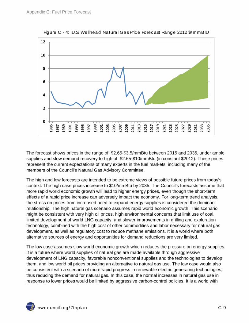
Appendix C: Fuel Price Forecast
nwcouncil.org/7thplan C-9
Figure C - 4: U.S. Wellhead Natural Gas Price Forecast Range 2012 $/mmBTU
The forecast shows prices in the range of $2.65-$3.5/mmBtu between 2015 and 2035, under ample supplies and slow demand recovery to high of $2.65-$10/mmBtu (in constant $2012). These prices represent the current expectations of many experts in the fuel markets, including many of the members of the Council’s Natural Gas Advisory Committee.
The high and low forecasts are intended to be extreme views of possible future prices from today’s context. The high case prices increase to $10/mmBtu by 2035. The Council’s forecasts assume that more rapid world economic growth will lead to higher energy prices, even though the short-term effects of a rapid price increase can adversely impact the economy. For long-term trend analysis, the stress on prices from increased need to expand energy supplies is considered the dominant relationship. The high natural gas scenario assumes rapid world economic growth. This scenario might be consistent with very high oil prices, high environmental concerns that limit use of coal, limited development of world LNG capacity, and slower improvements in drilling and exploration technology, combined with the high cost of other commodities and labor necessary for natural gas development, as well as regulatory cost to reduce methane emissions. It is a world where both alternative sources of energy and opportunities for demand reductions are very limited.
The low case assumes slow world economic growth which reduces the pressure on energy supplies. It is a future where world supplies of natural gas are made available through aggressive development of LNG capacity, favorable nonconventional supplies and the technologies to develop them, and low world oil prices providing an alternative to natural gas use. The low case would also be consistent with a scenario of more rapid progress in renewable electric generating technologies, thus reducing the demand for natural gas. In this case, the normal increases in natural gas use in response to lower prices would be limited by aggressive carbon-control policies. It is a world with
0
2
4
6
8
10
12
1985
19
87
1989
19
91
1993
19
95
1997
19
99
2001
20
03
2005
20
07
2009
20
11
2013
20
15
2017
20
19
2021
20
23
2025
20
27
2029
20
31
2033
20
35

Appendix C: Fuel Price Forecast
nwcouncil.org/7thplan C-10
substantial progress in efficiency and renewable technologies, combined with more stable conditions in the Middle East and other oil and natural gas producing areas.
The intermediate cases are variations on the medium case that are considered reasonably likely to occur. The medium-high case would contain elements of the high scenario, however not to the same degree. Similarly, the medium-low case would contain some of the more optimistic factors described for the low case.
In reality, prices may at various times in the future resemble any of the forecast range. Such cycles in natural gas prices, as well as shorter-term volatility, are captured in the Council’s Regional Portfolio Model. Table C - 1 shows the range of natural gas price trend forecasts for selected years. In the Council’s portfolio analysis, however, prices at any given time may fall anywhere within, or even outside, the range in figure C - 4.
For a more detailed year-by-year forecast of prices, please see the companion workbook from the Council website.
Companion Spreadsheet for 7th Plan with Demand Forecast Data (Regional and state level details on economic drivers, fuel prices, demand and load forecast)
available from following link: http://www.nwcouncil.org/energy/powerplan/7/technical
Northwest Natural Gas Supplies and Price
Given a forecast of U.S. level commodity prices, the next step is to estimate the cost of natural gas within the Pacific Northwest region and the rest of the Western United States. This is necessary because there is significant regional variation in natural gas prices.
Natural gas supplies for the Pacific Northwest come from two sources: the Western Canada Sedimentary Basin (WCSB) in Alberta and Northeastern British Columbia, and the U. S. Rocky Mountains. Natural gas from these areas is delivered into the region by two pipelines. The Williams Northwest Pipeline delivers supplies from the U.S. Rocky Mountains as well as down from Sumas at the B.C. border. The other pipeline is TransCanada Gas Transmission Northwest, which brings supplies from Alberta, through the Northwest and on down to the California border. Figure C - 5 illustrates the Northwest’s natural gas delivery system (figure adopted from 2014 Natural Gas Outlook).
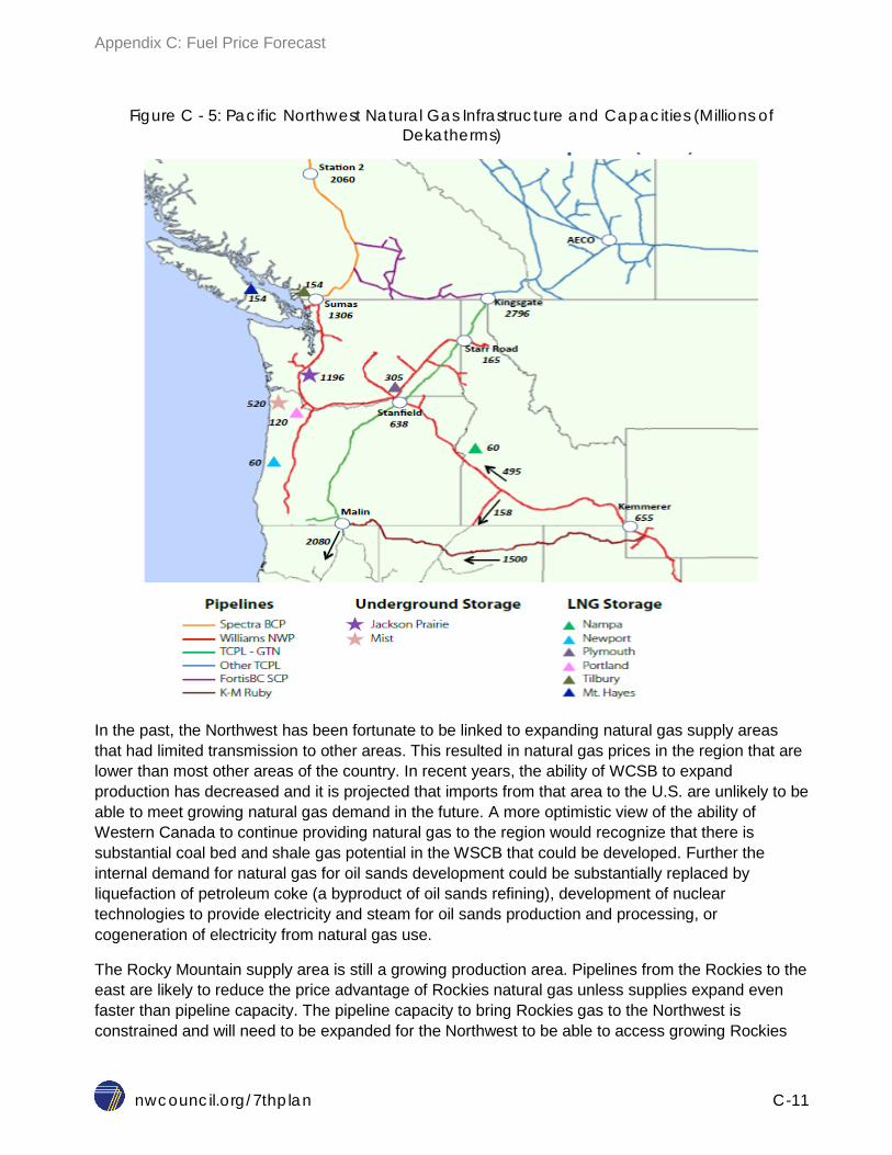
Appendix C: Fuel Price Forecast
nwcouncil.org/7thplan C-11
Figure C - 5: Pacific Northwest Natural Gas Infrastructure and Capacities (Millions of Dekatherms)
In the past, the Northwest has been fortunate to be linked to expanding natural gas supply areas that had limited transmission to other areas. This resulted in natural gas prices in the region that are lower than most other areas of the country. In recent years, the ability of WCSB to expand production has decreased and it is projected that imports from that area to the U.S. are unlikely to be able to meet growing natural gas demand in the future. A more optimistic view of the ability of Western Canada to continue providing natural gas to the region would recognize that there is substantial coal bed and shale gas potential in the WSCB that could be developed. Further the internal demand for natural gas for oil sands development could be substantially replaced by liquefaction of petroleum coke (a byproduct of oil sands refining), development of nuclear technologies to provide electricity and steam for oil sands production and processing, or cogeneration of electricity from natural gas use.
The Rocky Mountain supply area is still a growing production area. Pipelines from the Rockies to the east are likely to reduce the price advantage of Rockies natural gas unless supplies expand even faster than pipeline capacity. The pipeline capacity to bring Rockies gas to the Northwest is constrained and will need to be expanded for the Northwest to be able to access growing Rockies

Appendix C: Fuel Price Forecast
nwcouncil.org/7thplan C-12
supplies. It should be noted that with significant growth of Northeast production,, pipeline flows to the East from the Rockies as well as Canada are bring pushed back to the West, which will benefit those customers (in terms of supply and lower prices).
There is general agreement that natural gas will have to play an important role in electricity supplies for the Council’s planning horizon. The cost of that natural gas will depend on the demand for natural gas and the supply and deliverability to the region. The deliverability of natural gas depends not only on access to supplies and pipeline capacity, but also on storage capability and other natural gas peaking resources like line pack, LNG storage, and interruptible demand.
The growing use of natural gas for electricity generation will require increased coordination between the electricity and natural gas industries. This is particularly true for natural gas used for peaking generation or ancillary services. Natural gas is currently scheduled on a daily basis, but electricity is scheduled on an hourly basis with constant adjustment to actual demands through load following and regulation services. Increasing amounts, and perhaps different forms, of natural gas flexibility within the day may be required as the use of natural gas increases for providing flexibility and ancillary services for the electricity sector. There has been significant coordination of efforts between the Natural Gas Association members and electric utility representative organizations in the past few years, in large part due to coordination and communication requirements ordered by FERC. The Northwest Mutual Assistance Agreement helps coordinate regional response during gas emergencies. FERC is attentive to the growing gas and electric overlap and is considering synchronizing the gas and electric scheduling day. In order to plan for the region’s electricity needs, the Council must forecast natural gas prices, not only in the Northwest, but also in other areas of the West. To do this, the Council has developed relationships among the various natural gas pricing hubs in the West. Most relevant to the Northwest are prices at the AECO-NIT pricing hub in Alberta, the Sumas hub on the Washington-B.C. border, and the Rocky Mountain hub.
Forecasts of natural gas delivered to specific parts of the Pacific Northwest are based on the forecasts of hub prices at Sumas, AECO, and the Rockies plus estimated costs of transporting the fuel via regional pipelines. Pipeline costs include three general types of cost: capacity charges, commodity charges, and in-kind fuel costs. Capacity costs are by far the largest component of the transportation cost, and they are considered to be fixed costs. Existing users of natural gas are assumed to pay rolled-in pipeline capacity costs, but future power plants are assumed to pay incremental capacity costs, which reflect new pipeline capacity costs that escalate in real terms over time. The rate of escalation varies with the forecast case. Pipeline commodity and in-kind fuel charges are small and are a variable cost of natural gas, along with the cost of the gas itself.
For the full range of forecast prices for national and regional hubs, please see the companion spreadsheet provided as part of the Seventh Power Plan from Council’s website at: http://www.nwcouncil.org/energy/powerplan/7/technical

Appendix C: Fuel Price Forecast
nwcouncil.org/7thplan C-13
OIL Background
Forecasts of oil prices play a less direct role in the Council’s Power Plan than natural gas prices. Oil is not a significant fuel for electricity generation, nor is it an important competitor with electricity in end-use applications. However, oil prices do have an influence on natural gas prices and other energy sources. The relationship is not exact, but as shown in Figure C - 6, crude oil and natural gas commodity prices do tend to move together in the long-term. Oil is most significant as a transportation fuel. In that role, oil prices enter into determining delivered coal prices at various points in the West. This is due to the reliance on diesel fuel to run the trains that deliver coal from supply areas in Wyoming and Montana. In the 2011 world oil prices reached the highest level ever recorded. The price of $104 per barrel of oil (2012$) was six and half times the average price for a year in 1998. Then world oil price crashed in late 2014 and by first quarter of 2015 world oil prices have been hovering in the low $50-$60/barrel range.
Figure C - 6: Historical Comparison of Crude Oil and Wellhead Natural Gas Prices
Oil Price Forecast Range
The oil price forecast proposed here is somewhat different from the forecast included in the Council’s Six Power Plan. The medium forecast of world oil prices, defined as refiners’ acquisition cost of imported oil, varies between $53- $99/barrel (2012$), this range of price forecast reflects the collapse of oild prices in 2015 and delay in expected recovery. Slowdown in economic growth in China is expected to contribute to slower recovery in world oil prices.. Prices generally fall following a period of extremely high prices as new sources of supply, substitution of other energy sources, and reduced demand bring markets into balance. However, as oil production increases, more
-
20
40
60
80
100
120
-
1.0
2.0
3.0
4.0
5.0
6.0
7.0
8.0
9.0
1969
1971
1973
1975
1977
1979
1981
1983
1985
1987
1989
1991
1993
1995
1997
1999
2001
2003
2005
2007
2009
2011
2013
Wellhead Natural Gas Prices ($2012/MMBtu)
U.S. Crude Oil Acquisition Cost by Refiners (2012 Dollars per Barrel)
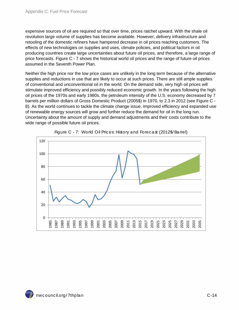
Appendix C: Fuel Price Forecast
nwcouncil.org/7thplan C-14
expensive sources of oil are required so that over time, prices ratchet upward. With the shale oil revolution large volume of supplies has become available. However, delivery infrastructure and retooling of the domestic refiners have hampered decrease in oil prices reaching customers. The effects of new technologies on supplies and uses, climate policies, and political factors in oil producing countries create large uncertainties about future oil prices, and therefore, a large range of price forecasts. Figure C - 7 shows the historical world oil prices and the range of future oil prices assumed in the Seventh Power Plan.
Neither the high price nor the low price cases are unlikely in the long term because of the alternative supplies and reductions in use that are likely to occur at such prices. There are still ample supplies of conventional and unconventional oil in the world. On the demand side, very high oil prices will stimulate improved efficiency and possibly reduced economic growth. In the years following the high oil prices of the 1970s and early 1980s, the petroleum intensity of the U.S. economy decreased by 7 barrels per million dollars of Gross Domestic Product (2005$) in 1970, to 2.3 in 2012 (see Figure C -8). As the world continues to tackle the climate change issue, improved efficiency and expanded use of renewable energy sources will grow and further reduce the demand for oil in the long run. Uncertainty about the amount of supply and demand adjustments and their costs contribute to the wide range of possible future oil prices.
Figure C - 7: World Oil Prices: History and Forecast (2012$/Barrel)
0
20
40
60
80
100
120
1985
19
87
1989
19
91
1993
19
95
1997
19
99
2001
20
03
2005
20
07
2009
20
11
2013
20
15
2017
20
19
2021
20
23
2025
20
27
2029
20
31
2033
20
35
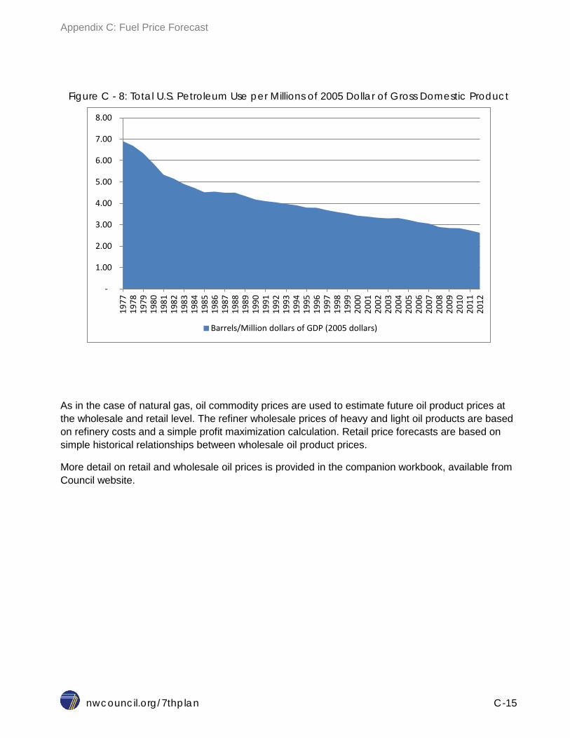
Appendix C: Fuel Price Forecast
nwcouncil.org/7thplan C-15
Figure C - 8: Total U.S. Petroleum Use per Millions of 2005 Dollar of Gross Domestic Product
As in the case of natural gas, oil commodity prices are used to estimate future oil product prices at the wholesale and retail level. The refiner wholesale prices of heavy and light oil products are based on refinery costs and a simple profit maximization calculation. Retail price forecasts are based on simple historical relationships between wholesale oil product prices.
More detail on retail and wholesale oil prices is provided in the companion workbook, available from Council website.
-
1.00
2.00
3.00
4.00
5.00
6.00
7.00
8.00 19
77
1978
19
79
1980
19
81
1982
19
83
1984
19
85
1986
19
87
1988
19
89
1990
19
91
1992
19
93
1994
19
95
1996
19
97
1998
19
99
2000
20
01
2002
20
03
2004
20
05
2006
20
07
2008
20
09
2010
20
11
2012
Barrels/Million dollars of GDP (2005 dollars)

Appendix C: Fuel Price Forecast
nwcouncil.org/7thplan C-16
COAL Coal Commodity Prices Coal is a plentiful energy source in the United States. Coal resources, like natural gas, are measured in many different forms. The EIA reports several of these.1 One measure is “demonstrated reserve base,” which measures coal more likely to be mined based on seam thickness and depth. EIA estimate as of January 2014, the demonstrated reserve base (DRB) was estimated to contain 480 billion short tons. In the United States, coal resources are larger than remaining natural gas and oil resources, based on total British thermal units (Btus). Annually, EIA reports remaining tons of coal in the DRB, which is comprised of coal resources that have been identified to specified levels of accuracy. EIA annually estimates recoverable coal reserves by adjusting the DRB to reflect accessibility and recovery rates in mining. As of January 1, 2014, EIA estimated that the remaining U.S. recoverable coal reserves totaled over 256 billion short tons, from a DRB of 480 billion short tons.
About half of the demonstrated reserve base of coal, 480 billion short tons, and 160 billion short-tons of recoverable reserves out of 256 billion short-tons nationally is located in the West. Western coal production has been growing due to several advantages it has over Appalachian and interior deposits. Western coal, especially Powder River Basin coal, is cheaper to mine due to its relatively shallow depths and thick seams. More important, Western coal is lower in sulfur content. Use of low-sulfur coal supplies has been an attractive way to help utilities meet increased restrictions on sulfur dioxide emissions under the 1990 Clean Air Act Amendments that took effect on January 1, 2000. The other characteristic that distinguishes most Western coal from Eastern and interior supplies is its Btu content. Western coal is predominately sub-bituminous coal with an average heat content of about 17 million Btu’s per short ton. In contrast, Appalachian and interior coal tends to be predominately higher grade bituminous coal with heat rates averaging about 24 million Btu per short ton. Another drawback of some Western coal is a relatively high arsenic content, which will require more expensive treatment for removal under stricter environmental rules.
Western coal production in 2013 was 528 million short tons, with 74 percent of that production coming from Wyoming (388 million short tons). The second largest state producer was Montana at 42 million tons. Colorado, New Mexico, North Dakota and Utah produced between 22 and 28 million short tons each, and Arizona produced about 8 million short tons.2
Historical productivity increases have been rapid, especially in Western coal mines. As a result, mine-mouth coal prices have decreased over time. In constant dollars, Western mine-mouth coal prices declined by an average of 1.6 percent per year between 1985 and 2005. Expiring higher-priced long-term contracts have also contributed to declining coal prices.
1 U.S. Energy Information Administration, U.S. Coal Reserves: Update, January 2014. 2 U.S. Energy Information Administration, EIA Interactive Coal Report, April 2015.
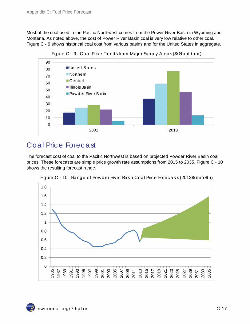
Appendix C: Fuel Price Forecast
nwcouncil.org/7thplan C-17
Most of the coal used in the Pacific Northwest comes from the Power River Basin in Wyoming and Montana. As noted above, the cost of Power River Basin coal is very low relative to other coal. Figure C - 9 shows historical coal cost from various basins and for the United States in aggregate.
Figure C - 9: Coal Price Trends from Major Supply Areas ($/Short tons)
Coal Price Forecast The forecast cost of coal to the Pacific Northwest is based on projected Powder River Basin coal prices. These forecasts are simple price growth rate assumptions from 2015 to 2035. Figure C - 10 shows the resulting forecast range.
Figure C - 10: Range of Powder River Basin Coal Price Forecasts (2012$/mmBtu)
0 10 20 30 40 50 60 70 80 90
2001 2013
United States Northern Central Illinois Basin Powder River Basin
0
0.2
0.4
0.6
0.8
1
1.2
1.4
1.6
1.8
1985
19
87
1989
19
91
1993
19
95
1997
19
99
2001
20
03
2005
20
07
2009
20
11
2013
20
15
2017
20
19
2021
20
23
2025
20
27
2029
20
31
2033
20
35

Appendix C: Fuel Price Forecast
nwcouncil.org/7thplan C-18
More detail on retail and wholesale oil prices is provided in the companion workbook, available on the Council’s website.
METHODOLOGY From Source to Burnertip Methodology for taking the source/hub prices and estimating burner-tip prices for coal and oil did not change for the Seventh Power Plan. For a detail look at the methodology for estimating the burner-tip fuel prices please see Appendix A-6 of the Sixth Power Plan. The methodology for estimating burner-tip natural gas prices was enhanced in the Seventh Power Plan. The relationship between burner-tip prices and hub prices were developed using EIA data (utility purchased price of gas at state level or at plant level). A summary of these relationships are shown in Table C - 1. Starting with the forecast of wellhead prices, described earlier in this appendix, the Council calculated the forecast of prices at Henry hub. Then, using relationship between various hubs and Henry Hub, the Council estimated prices for other hubs. In the third stage, the Council estimated burner-tip prices at target locations (based on Aurora wholesale market price model’s topology). Then, this price forecast was further enhanced by developing monthly price shapes using historic monthly price data from 2000-2012 (see Table C - 2). The monthly shapes show ratio of a monthly price to annual price.
Table C - 1: Relationship between Wellhead, Henry Hub and Burner-tip prices
HENRY
AECO ROCKIES SUMAS SAN_JUAN PERMIAN Source Hub Wellhead Henry Henry Henry Henry Henry Coeff. For Hub 1.04 1.02 0.83 0.90 0.87 0.92 Constant - (0.94) - - - -
Burner-tip
Located at PNW_EAST MTE CA_N NV_N AB UT WY Source Hub AECO Rockies AECO AECO AECO Rockies Rockies Coeff. For Hub 1.03 0.87 0.53 1.13 1.00 0.74 1.00 Constant - 2.19 2.76 1.05 (0.24) 1.67 0.47
Burner-tip Located at PNW_WEST ID_S BC CO CA_S AZ NM NV_S
Source Hub AECO Rockies AECO Rockies San Juan San Juan Permian Permian
Coeff. For Hub 1.03 0.55 1.00 0.74 1.05 0.96 0.90 1.02 Constant (0.05) 4.67 0.24 1.74 1.01 1.01 1.12 -
Additional information can be located in the supporting file located at: http://www.nwcouncil.org/energy/powerplan/7/technical

Appendix C: Fuel Price Forecast
nwcouncil.org/7thplan C-19
Table C - 2: Monthly Shape of Prices Monthly Shapes AZ CA CO NM NV OR
January 1.03 1.04 1.05 1.05 1.13 1.10 February 1.03 1.01 1.09 1.01 1.05 1.01 March 0.96 1.01 1.07 0.98 1.08 1.00 April 0.98 0.97 1.01 0.96 0.97 1.00 May 0.99 0.98 0.92 0.97 0.97 1.10 June 1.00 1.00 1.00 1.01 0.96 0.98 July 1.01 0.99 0.99 1.03 0.95 0.94 August 0.96 0.96 0.97 0.95 0.96 0.90 September 0.92 0.93 0.83 0.92 0.97 0.86 October 0.97 0.99 0.95 0.97 0.96 0.92 November 1.02 1.00 1.00 1.06 0.95 1.05 December 1.14 1.09 1.11 1.07 1.05 1.15
Monthly
Shapes UT WA WY ID MT January 1.09 1.16 1.13 1.17 1.12 February 1.13 0.98 1.14 1.14 1.07 March 1.14 0.97 0.99 1.32 1.02 April 0.98 1.24 0.88 0.91 0.91 May 0.95 1.10 1.10 1.06 0.92 June 0.97 1.08 0.91 1.09 1.02 July 1.03 0.90 1.05 0.96 1.12 August 0.96 0.89 0.90 0.90 1.01 September 0.87 0.88 0.88 0.76 0.86 October 1.00 0.90 0.81 0.78 0.80 November 1.00 0.99 1.16 0.92 1.09 December 0.87 0.97 1.03 1.00 1.05
Monthly Shapes NV_N NV_S CA-S CA-N PNW-E
PNW-W ID-S
January 1.13 1.03 1.00 1.05 1.06 1.15 1.09 February 1.06 1.04 0.99 1.02 1.01 1.02 1.06 March 1.05 1.11 0.99 1.01 0.99 0.92 1.10 April 0.97 0.91 0.97 0.96 0.99 1.06 0.96 May 0.99 0.93 1.00 0.97 1.18 0.99 1.00 June 0.96 0.95 1.00 0.97 0.92 1.06 1.03 July 0.94 1.07 1.01 0.99 0.98 0.96 0.96 August 0.98 0.95 0.98 0.95 0.93 0.92 0.97 September 0.98 0.84 0.93 0.95 0.92 0.86 0.90 October 0.95 0.92 0.95 0.98 0.93 0.88 0.91 November 0.99 0.96 1.06 1.05 1.03 1.00 0.97 December 1.00 1.26 1.13 1.10 1.07 1.19 1.04
Seventh Northwest Conservation and Electric Power Plan
nwcouncil.org/7thplan D-1
APPENDIX D: ECONOMIC FORECAST
Contents Role Of the Economic Forecast ......................................................................................................... 4 Background ....................................................................................................................................... 5
Economic Growth Assumptions ..................................................................................................... 5 Economic Drivers of Residential Demand......................................................................................... 5
Population ...................................................................................................................................... 6 Housing Stock ................................................................................................................................ 8 Personal Income .......................................................................................................................... 16 Number of Energy-using Appliances in the Average Residence .................................................. 17
Information Communication and Entertainment ........................................................................ 17 Demand for Air Conditioning .................................................................................................... 21
Economic Drivers of the Commercial Sector ................................................................................... 23 Methodology in Estimating Commercial Floor Space Requirements ............................................ 23
Square Footage per Employee ................................................................................................. 25 Forecasting Commercial Floor Space Requirements ................................................................... 26 Changing Composition of Commercial Sector .............................................................................. 27 Commercial Floor Space Additions .............................................................................................. 29
Patterns of Commercial Floor Space Additions ........................................................................ 31 Commercial Floor Space Stock .................................................................................................... 34
Economic Drivers for Industrial Sector Demand .............................................................................. 35 Projected Employment Growth .................................................................................................... 36 Industrial Output .......................................................................................................................... 37
Economic Drivers for other Sectors ................................................................................................. 40 Irrigation ....................................................................................................................................... 40 Transportation .............................................................................................................................. 40
Alternative Economic Scenarios ...................................................................................................... 41
List of Figures and Tables
Figure D - 1: Population Forecast (000) ............................................................................................ 7 Table D - 1: Population in the Region (000) ...................................................................................... 8 Table D - 2: Composition of Regional Population (000) .................................................................... 8 Figure D - 2: Declining Household Size (People per Household) ...................................................... 9 Figure D - 3: Growing Average Size of New Single Family Homes ................................................... 9 Table D - 3: Average size of residential units (sqf)........................................................................... 10 Figure D - 4: Historic and future composition of Housing Stock in the Northwest ............................. 11 Figure D - 5: Number of Single-Family Homes (000) Stock ............................................................ 11 Figure D - 6: Number of Multi-Family Homes (000) Stock ............................................................... 12

Appendix D: Economic Forecast
nwcouncil.org/7thplan D-2
Figure D - 7: Number of Manufactured Homes (000) Stock ............................................................ 12 Figure D - 8: New Manufactured Homes per Year .......................................................................... 13 Figure D - 9: New Multifamily Homes per Year ............................................................................... 13 Figure D - 10: New Single Family additions per Year ..................................................................... 14 Table D - 4: Market share by building type ...................................................................................... 14 Table D - 5: Regional Multifamily New Additions Market share ........................................................ 14 Table D - 6: Average Annual Number of New Homes by State ....................................................... 15 Table D - 7: Historic and forecast stock of residential units (1000s) ................................................ 16 Table D - 8: Growth Rate Personal Income (2000 constant dollars) ............................................... 16 Figure D - 11: Personal Income ...................................................................................................... 16 (Billions in 2005 constant dollars) .................................................................................................... 16 Figure D - 12: Count of Computers per household .......................................................................... 18 Figure D - 13: Percent of Households with Computers .................................................................... 18 Figure D - 14: TV screen type by Vintage of TV .............................................................................. 19 Figure D - 15: Number of TVs per home .......................................................................................... 19 Figure D - 16: Estimated consumption, in average MW, for select miscellaneous uses ................... 20 Table D - 9: Estimated consumption, in average MW, for select miscellaneous uses ...................... 20 Table D - 10: Annual Shipment of Room Air Conditions to the Region (number) ............................ 21 Figure D - 17: Recent Trends in Nationwide Shipment of Room Air Conditioners (1000s) ............. 22 Table D - 11: 2014 Commercial Building Stock (1,000,000 SQF) ................................................... 25 Figure D - 18: Median square footage per employee ...................................................................... 26 Figure D - 19: Commercial Employment Projection (thousands) ..................................................... 27 Table D - 12: Number of employees in the commercial enterprises ................................................. 28 Table D - 13: Percent Market Share of Employment ....................................................................... 28 Figure D - 20: 2013 Stock of Commercial floor space by Business type (millions sqft) .................... 29 Figure D - 21: Total Commercial Floor Space Additions (Millions of SQFT) .................................... 30 Table D - 14: 2015-2035 New Commercial Floor Space Additions (millions of sqf) ......................... 31 Figure D - 22: Pattern of Office Space Addition (millions of sqf) ..................................................... 32 Figure D - 23: Pattern of Retail Space Addition (millions sqf) ......................................................... 32 Figure D - 24: Pattern of Warehouse Floor Space Additions (millions of sqf) .................................. 33 Figure D - 25: Pattern of Floor Space Addition for K-12 Schools (million sqf) ................................. 33 Figure D - 26: Pattern of Floor Space Addition for Elder Care Facilities (million sqf) ....................... 34 Table D - 15: Regional Commercial Floor Space Stock (millions sqf) ............................................. 35 Figure D - 27: Change in Regional Energy Intensity ....................................................................... 36 Figure D - 28: Employment in Manufacturing Sectors (1000s) ........................................................ 37 Figure D - 29: Average Annual Percent Change in non-farm Business sector (National Data) ........ 38 Figure D - 30: Average Annual Percent Change in Manufacturing sector (National Data) ............... 38 Figure D - 31: National improvement in Labor Productivity 1987 and 2012 indexed to 2000 .......... 39 Table D - 16: Regional Industrial Output (billions of $2012) ............................................................ 40 Table D - 17: Forecast number of new vehicle additions and assumed market share of electric vehicles ........................................................................................................................................... 41 Table D - 18: Historic and Forecast of Annual Growth Rate by Sector ............................................ 43 Table D - 19: Forecast of Range of Annual Growth Rate by Sector ................................................ 44

Appendix D: Economic Forecast
nwcouncil.org/7thplan D-3
In the bulk of this write-up we have presented the medium range of the forecast. At the last section we present the range of uncertainty on the drivers. This is done to reinforce the fact that future is uncertain. Council’s planning process does not use a single deterministic future to drive the analysis. The stochastic variation introduced in the Regional Portfolio Model tests a wide range of future uncertainties in load, fuel prices etc.

Appendix D: Economic Forecast
nwcouncil.org/7thplan D-4
ROLE OF THE ECONOMIC FORECAST A 20-year forecast of demand for electricity is one of the requirements of the Northwest Power Act (Public Law 96-501, Sec. 4(e)(3)(D) ). A detailed demand forecast is used in planning future conservation potential, electricity market clearing price projections, as well as in the Council’s own resource risk assessments. To better capture the impact of future uncertainties, the Council develops a forecast of future demand for energy that identifies not just one trend but a range of trends. The demand forecast range is determined by a consistent set of assumptions about uncertainties in future economic and demographic activities in the region (focus of this chapter), the trajectory of fossil fuel and electricity prices, and legislative and market responses to climate change.
The figure below depicts the Council’s power planning process. The planning process starts with economic and demographic assessments and then adds fuel and electricity price forecasts to create a forecast for electricity demand. The demand forecast looks at energy use by sector to predict monthly load for electricity generators. The Northwest load forecast, along with the forecast for load outside the Northwest, is used in forecasting wholesale electricity prices. Northwest load is used in the Council’s Regional Portfolio Model (RPM), which is then used to seek least-cost, low-risk resource options for the region to meet that load.
The demand forecast is also used extensively to develop the conservation supply curves. The key economic drivers for the conservation supply curves are identical to the economic drivers of the demand forecast.
NorthwestPower andConservation
Council
Council’s Power Planning Process
Economic & Demographic
Forecasts
Fuel PriceForecasts
ConservationPrograms and
Costs
GeneratingResources and
Costs
Demand Forecasting System
Residential Commercial Industrial Irrigation
Total Electricity Use
Supply - Demand Balance
Resource Supply(Cost and Amount)
ElectricityPrice

Appendix D: Economic Forecast
nwcouncil.org/7thplan D-5
BACKGROUND Economic Growth Assumptions The national economic models driving the regional forecast of the Seventh Power Plan were updated as of the fourth quarter of 2014. Given the long-term nature of the Council’s power plan, many factors determine the load forecast. Long-term variables may be economic circumstances, life-style choices, demographic changes, or socio-economic trends that take decades to develop and fade. Energy demand is also affected by short-term factors, such as weather conditions or changes in income. The combination of all these conditions determines the demand for energy.
ECONOMIC DRIVERS OF RESIDENTIAL DEMAND The number of dwellings is a key driver of energy demand in the residential sector. Residential demand begins with the number of units, including single family, multifamily, and manufactured homes. The “number of homes” category is driven by regional population, house size, and composition of the population. The region’s population increased from about 8.9 million in 1985 to about 13 million by 2010, and is projected to grow to over 16 million by 2035 at an annual rate of 0.9 percent.
In the residential sector, electricity demand is driven by space and water heating, space cooling, refrigeration, cooking, washing and a new category called Information, Communication and Entertainment (ICE). This new category includes all portable devices that must be charged, such as laptop computers and cell phones, as well as larger, more energy-intensive televisions and gaming devices. As the regional population grows and with it the number of new homes, demand for these services and as well as other appliances will all increase. While this growth will be slower due to improvements in the energy efficiency of new appliances as a result of state and federal standards, energy demand, overall growth in the number of households will increase demand.
In addition to the number of devices and appliances in homes that consume electricity, another factor affecting residential demand for electricity changing life-styles. For example, the saturation rate for air-conditioning and other appliances and electronic equipment is increasing. Over 80 percent of all new homes in the region now have central air conditioning. This compares to 7 to 8 percent of housing stock with central air conditioning in the 1980s. The growth in high-speed Internet access has increased electricity demand from home electronics which grew at a rate of over 6 percent per year since 2000.

Appendix D: Economic Forecast
nwcouncil.org/7thplan D-6
Population The region’s population is changing and reflects demographic shifts seen throughout the United States. In 1985, 30 percent of the region’s population was younger than 19. This age group has been growing at about 1 percent per year, but it is forecast to grow more slowly for the next two decades, at around 0.7 percent annually. As a percentage of the total population, it is projected to represent about 24 percent of the population by 2035. This generation represents consumers who have grown up with ICE technologies, the fastest-growing segment of residential electricity demand.
The 20 to 64 year-old age group, representing the working age population, has grown from about 5 million in 1985 to about 8 million in 2010, and is projected to grow to over 9 million by 2035. This age group has been growing at 1.6 percent per year, but its growth rate is expected to be significantly reduced as more and more baby boomers retire. This demographic category plays a critical role in regional employment, demand for homes, major capital equipment, and goods and services.
The fastest-growing population segment is people over 64, the “retirees.” They represented about 12 percent of the population in 1985, and by 2035 they are expected to represent about 20 percent of the region’s population. This segment is expected to grow almost 2.3 percent per year over the next 20 years, at almost two and half times the growth rate of the total population. This trend has affected the commercial sector in many ways, and the increase in the number of businesses catering to elders is one example. In 2005, the Bureau of Labor Statistics and county business patterns show there were over 3,200 businesses in the region offering elder care services. Such businesses had more than 100,000 employees and occupied about 178 million square feet of space by 2015. If the current trends continue, by 2035 an additional 54 million square feet of space would be needed for elder care. The demand from this business is tracked in the commercial section of the model.
The Figure D – 1 shows the expected population change in each of the four states. Table D – 1 shows the population forecast for each of the states in the region as well as the annual growth rates used in the Seventh Plan. Table D – 2 shows the age composition of the Northwest’s population through time.

Appendix D: Economic Forecast
nwcouncil.org/7thplan D-7
Figure D - 1: Population Forecast (000)
-
2,000
4,000
6,000
8,000
10,000
12,000
14,000
16,000
18,000
1990 2000 2010 2020 2030 2035
State Population - Historic and Projection(1000s)
Idaho Montana Oregon Washington

Appendix D: Economic Forecast
nwcouncil.org/7thplan D-8
Table D - 1: Population in the Region (000)
Annual Growth rates1
State 1990 2000 2010 2020 2030 2035 1985-2014 2015-2035
ID 1,017 1,302 1,572 1,770 2,015 2,136 1.7% 1.3% MT 802 904 992 1,077 1,129 1,149 0.8% 0.5% OR 2,869 3,435 3,841 4,192 4,527 4,678 1.4% 0.8% WA 4,916 5,921 6,753 7,506 8,159 8,460 1.6% 0.9%
Region 9,603 11,561 13,158 14,546 15,830 16,423 1.5% 0.9%
Table D - 2: Composition of Regional Population (000)
Population Cohort
1990 2000 2010 2020 2030 2035
AAGR
1985-2014
AAGR
2015-2035
Age 0 thru 19 2,824 3,301 3,463 3,571 3,800 3,925 0.9% 0.6% Age 20 thru 64 5,580 6,886 7,973 8,467 8,971 9,245 1.6% 0.6% Age 65 &over 1,200 1,374 1,722 2,508 3,059 3,254 2.3% 2.2%
Housing Stock While the regional population has been increasing, the number of occupants per household has been declining. In 1985, the average household size was about 2.6 to 2.9 persons per household, and by 2035 it is expected to go down to 2.3 to 2.5 persons per household, resulting in the number of homes growing at a faster rate than the population. Figure D-2 shows the historical trend is household size from 1985 with projections through 2035.
1 Important note: This appendix uses average annual growth rates as summary figures when comparing the historic and forecast periods for many economic drivers and fuel prices. The average annual growth rate is sensitive to the base year values used in calculating the annual growth rates. For a more accurate picture of the year-by-year growth in economic drivers and prices, additional information for each state is available from the companion Excel worksheet available from Council’s website. This companion data can provide a more accurate picture of historic and future growth.
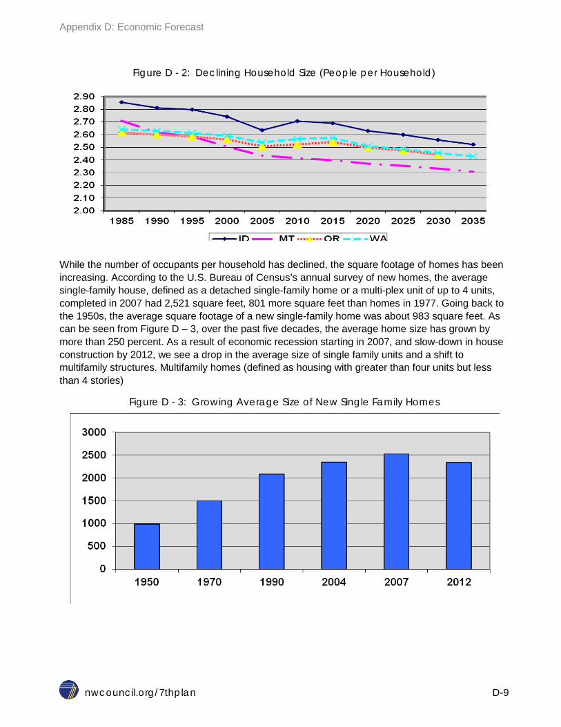
Appendix D: Economic Forecast
nwcouncil.org/7thplan D-9
Figure D - 2: Declining Household Size (People per Household)
While the number of occupants per household has declined, the square footage of homes has been increasing. According to the U.S. Bureau of Census’s annual survey of new homes, the average single-family house, defined as a detached single-family home or a multi-plex unit of up to 4 units, completed in 2007 had 2,521 square feet, 801 more square feet than homes in 1977. Going back to the 1950s, the average square footage of a new single-family home was about 983 square feet. As can be seen from Figure D – 3, over the past five decades, the average home size has grown by more than 250 percent. As a result of economic recession starting in 2007, and slow-down in house construction by 2012, we see a drop in the average size of single family units and a shift to multifamily structures. Multifamily homes (defined as housing with greater than four units but less than 4 stories)
Figure D - 3: Growing Average Size of New Single Family Homes

Appendix D: Economic Forecast
nwcouncil.org/7thplan D-10
The increase in the average size of homes has not been limited to single-family residences. It is difficult to predict the future trends in house size. For the Seventh Power Plan, the Council has assumed the dwelling sizes shown in Table D - 3. The data for 2014 comes from the recent Residential Building Stock Assessment.2
Table D - 3: Average size of residential units (sqf)
State Building type 1985 2014 2035 ID Single Family 2127 2174 2200 MT Single Family 2225 2270 2229 OR Single Family 1908 1973 1944 WA Single Family 2051 2140 2150 ID Multifamily 688 750 780 MT Multifamily 688 737 771 OR Multifamily 688 740 768 WA Multifamily 688 741 768 ID Other Family* 1160 1279 1288 MT Other Family 1339 1478 1492 OR Other Family 961 1203 1214 WA Other Family 1160 1273 1257
*- other family structures are manufactured homes
In absolute terms, the number of housing units has been growing at a faster pace than the overall population. Between 1985 and 2012, the population grew at 1.5 percent per year and the number of single family homes grew at 1.5 percent per year, with multifamily and manufactured homes growing at 2.2 to 2.3 percent per year, respectively. The future outlook for growth in homes coincides with slower projection for growth in population.
Figure D – 4 shows the historic and forecast mix of housing types in the total Northwest stock from 1985 through 2035. This figures shows that the share of single family homes declines gradually between 1985 and 1995, then remains fairly constant over the remaining period.
2 http://neea.org/resource-center/regional-data-resources/residential-building-stock-assessment
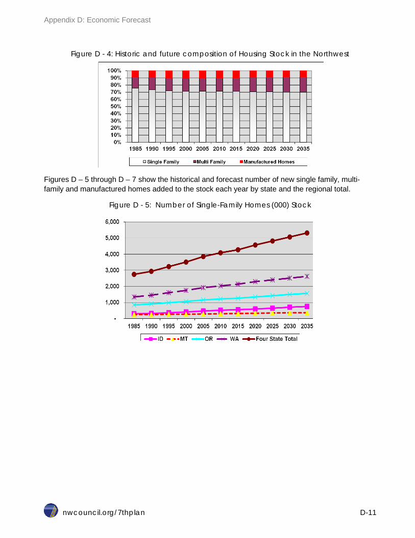
Appendix D: Economic Forecast
nwcouncil.org/7thplan D-11
Figure D - 4: Historic and future composition of Housing Stock in the Northwest
Figures D – 5 through D – 7 show the historical and forecast number of new single family, multi-family and manufactured homes added to the stock each year by state and the regional total.
Figure D - 5: Number of Single-Family Homes (000) Stock
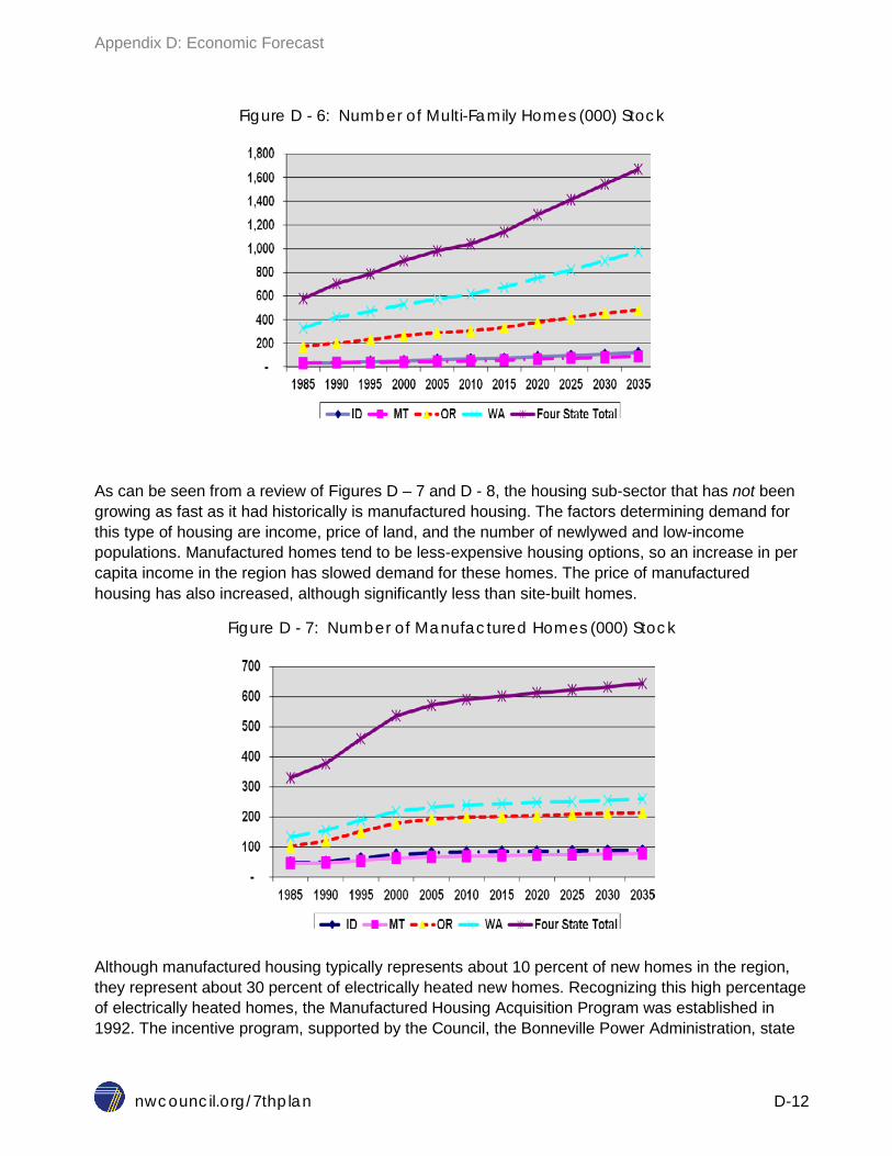
Appendix D: Economic Forecast
nwcouncil.org/7thplan D-12
Figure D - 6: Number of Multi-Family Homes (000) Stock
As can be seen from a review of Figures D – 7 and D - 8, the housing sub-sector that has not been growing as fast as it had historically is manufactured housing. The factors determining demand for this type of housing are income, price of land, and the number of newlywed and low-income populations. Manufactured homes tend to be less-expensive housing options, so an increase in per capita income in the region has slowed demand for these homes. The price of manufactured housing has also increased, although significantly less than site-built homes.
Figure D - 7: Number of Manufactured Homes (000) Stock
Although manufactured housing typically represents about 10 percent of new homes in the region, they represent about 30 percent of electrically heated new homes. Recognizing this high percentage of electrically heated homes, the Manufactured Housing Acquisition Program was established in 1992. The incentive program, supported by the Council, the Bonneville Power Administration, state

Appendix D: Economic Forecast
nwcouncil.org/7thplan D-13
energy offices, electric utilities, and manufacturers, paid manufacturers the incremental cost to add efficiency measures to each new home. New manufactured homes peaked in 1995 after this program ended. For now, the stock of manufactured homes is projected to increase, although at a slower rate.
The recent Residential Building Stock Assessment (2012) shows that on a square footage basis, existing stock of manufactured housing consumes more electricity and natural gas than single family homes. This issue will be discussed further in the demand forecast Appendix E.
Figure D - 8: New Manufactured Homes per Year
Figures D – 9 and D – 10 show the Seventh Plan’s medium forecast for new multifamily and single family homes. As can be seen from a review of these figures the number of new single family and multifamily homes added each years is anticipated to recover from pre-recession levels by 2015.
Figure D - 9: New Multifamily Homes per Year

Appendix D: Economic Forecast
nwcouncil.org/7thplan D-14
Figure D - 10: New Single Family additions per Year
As can be observed from Table D – 4, the overall composition of housing stock has recently been changing to favor multifamily homes. Although single-family homes had been increasing in market share in the late twentieth century, recent trends are that they are gradually losing market share. Single-family homes represented 47 percent of homes in the region in 1985. By 2015 they are expected to represent 66 percent of housing stock. However, by 2035, the forecast is for single-family homes to decline to about 64 percent. Multifamily homes represented 34 percent of residential housing stock in 1985, 18 percent by 2000, and are projected to be about 27 percent of the total housing stock by 2035. Within the multifamily building type, high rise structures have been and are projected to continue to represent a larger share. Table D – 5 shows that within high-rise buildings, those with four stories and above, are projected to constitute about 18 percent of multifamily housing stock by 2035, nearly doubling of their market share in from 1985-2000. Manufactured homes historically represented 12 to 17 percent of the housing stock, but this building type’s market share is projected to decrease to around 3 percent by 2035.
Table D - 4: Market share by building type
1985 2000 2015 2030 2035 Single Family 47% 67% 66% 64% 64% Multifamily - Low Rise 34% 18% 26% 28% 27% MF - High Rise 2% 3% 6% 6% 6% Manufactured Housing 17% 12% 2% 3% 3%
Table D - 5: Regional Multifamily New Additions Market share
1985-2000 2001-2006 2007-2014 2015-2035 Low rise 90% 86% 84% 82% High rise 10% 14% 16% 18%
-10,000 20,000 30,000 40,000 50,000 60,000 70,000 80,000 90,000
100,000
1985 1990 1995 2000 2005 2010 2015 2020 2025 2030 2035
ID MT OR WA Four State-Total

Appendix D: Economic Forecast
nwcouncil.org/7thplan D-15
Table D - 6 shows changing market share of various residential building types across different historic and forecast periods. On average, between 1985 and 2000, about 50,000 new single-family, 19,000 low-rise multifamily and 2,000 high-rise multifamily, and 14,000 new manufactured homes were added to the existing stock. Starting in year 2000 and lasting until 2006, each year has seen a dramatic increase in new single-family home additions. Rising income levels in the region and the increased availability of credit caused a shift from multifamily to single-family home ownership. In 2001-2006, more than 70,000 new single-family homes were added in the region. This increase in the number of single-family houses caused a substantial increase in the price of housing. A slow-down in new single-family home additions is evident in the 2007-2014 period with almost half as many built as during the previous 5 year period. For the forecast period 2015-2035, the Council predicts a return to more stable level of construction.
Table D - 6: Average Annual Number of New Homes by State
1985-2000 2001-2006 2007-2014 2015-2035
Single-Family Idaho 6,987 13,743 5,828 10,518 Montana 1,706 3,547 2,344 2,650 Oregon 13,674 19,392 8,219 15,170 Washington 26,952 33,992 18,839 24,004 Four State Total 49,319 70,674 35,230 52,342 Multifamily- Low rise Idaho 1,144 1,559 828 1,844 Montana 547 855 760 1,410 Oregon 4,998 3,439 2,242 6,069 Washington 12,539 8,430 7,632 12,397 Four State Total 19,228 14,283 11,462 21,721 Multifamily- high rise Idaho 88 127 96 420 Montana 51 78 85 317 Oregon 1,157 1,336 1,179 1,330 Washington 895 826 800 2,827 Four State Total 2,192 2,367 2,160 4,893 Manufactured Housing Idaho 1,818 873 357 270 Montana 1,161 778 393 363 Oregon 4,983 2,424 870 670 Washington 5,609 2,809 1,037 795 Four State Total 13,571 6,884 2,657 2,098
In summary, the key driver for demand for electricity consumption in the residential sector is the number of residential units. Table D - 7 presents the existing residential units for select years.

Appendix D: Economic Forecast
nwcouncil.org/7thplan D-16
Table D - 7: Historic and forecast stock of residential units (1000s)
Regional Summary 1985 2007 2015 2020 2030 2035 Single Family 2,753 3,997 4,279 4,573 5,077 5,318 Multi Family 578 1,016 1,141 1,286 1,546 1,673 Manufactured homes 329 583 601 611 632 643
Personal Income Personal income is another economic driver of energy demand. Energy consumption is elastic, so a decline in personal income causes a short-term reduction in demand. Regional personal income, both in total and on a per-capita basis, has been on the upswing and is projected to continue, although at a slower rate. Table D - 8 shows the growth rate, in constant dollars, for personal income in the four states. Figure D – 11 shows the growth in personal income by state from 1985 to through the present and forecast to 2035.
Table D - 8: Growth Rate Personal Income (2000 constant dollars)
1985-2009 2010-2030 Idaho 3.9% 3.1% Montana 2.7% 2.4% Oregon 3.3% 2.9% Washington 3.8% 2.9% Four State- Total 3.6% 2.9%
Figure D - 11: Personal Income
(Billions in 2005 constant dollars)

Appendix D: Economic Forecast
nwcouncil.org/7thplan D-17
Number of Energy-using Appliances in the Average Residence Energy-using appliances also affect energy demand in the residential sector, and the penetration rate of appliances is a key driver of demand. One group of devices that has experienced significant growth in the residential sector has been home electronics (ICE). Very few sources track the penetration rate of this end-use at the regional level, so the following analysis draws on national-level data.
Information Communication and Entertainment
The explosive growth of these devices has been global, fueled in part by the rapid expansion of the Internet. In a not too distant past, the typical appliances in a typical home consisted of one or two refrigerators; a water heater; perhaps a freezer; some form of space-heating appliance; a cooking appliance; lighting fixtures; and, rarely, an air-conditioning unit. Entertainment appliances were usually limited to a color television and a stereo system.
An average home today has all these appliances, as well as a whole range of ICE devices. Some ICE devices provide services that were once performed outside the home, such as printing pictures or reports. Other ICE devices connect people to the outside world and social networks, and some provide entertainment. ICE devices, to a great extent, have removed the boundary between office work and home life as more and more people are able to conduct office work from home.
ICE end-uses are numerous and vary from household to household, depending on the life-style and demographic characteristics of the households In 2012 Northwest Energy Efficiency Alliance conducted an extensive survey of inventory of ICE appliances in the residential units. In the following charts, the Council is presenting some of the highlights of the NEEA survey findings. Readers are encouraged to read the full NEEA Residential Building Stock Assessment available through NEEA website linked below.
http://neea.org/resource-center/regional-data-resources/residential-building-stock-assessment

Appendix D: Economic Forecast
nwcouncil.org/7thplan D-18
Figure D - 12: Count of Computers per household
Figure D - 13: Percent of Households with Computers
0.0 0.5 1.0 1.5 2.0
ID
MT
OR
WA
Region
75% 80% 85% 90% 95%
ID
MT
OR
WA
Region

Appendix D: Economic Forecast
nwcouncil.org/7thplan D-19
Figure D - 14: TV screen type by Vintage of TV
Figure D - 15: Number of TVs per home
Using RBSA findings along with national and regional projections on various ICE appliances, the Council has developed a more detail forecast for this category of end uses than in previous power plans. Table D – 9 and Figure D -16 shows the rapid increase in demand for electricity from ICE end-uses, as well as projected reduction in their rate of growth over the next two decades.
0% 10% 20% 30% 40% 50% 60% 70% 80% 90%
100%
CRT Flat Screen
0 0.5 1 1.5 2 2.5
ID
MT
OR
WA
Region

Appendix D: Economic Forecast
nwcouncil.org/7thplan D-20
Figure D - 16: Estimated consumption, in average MW, for select miscellaneous uses
Table D - 9: Estimated consumption, in average MW, for select miscellaneous uses
1985 1990 1995 2000 2005 2010 2015 2030 2035 Color TV 86 111 136 159 200 270 218 126 123 Set top box - - - 43 112 164 144 189 224 Desktop computer 2 3 17 34 144 293 300 130 78 Computer Monitors 4 16 30 46 65 84 75 54 54 Lap-top Computers - - - - 8 17 36 26 22 Game Consoles 0 2 3 3 5 21 47 42 37 DVD - - - 3 10 25 24 9 6 VCR 12 17 23 27 29 - - - - Ceiling Fan 1 4 6 8 10 12 11 10 9 External Power Supply - 4 8 14 21 27 16 15 15 Audio 29 34 41 54 68 83 96 103 102 Security system 1 2 3 4 4 5 6 11 11 Microwave 26 42 55 60 64 68 72 84 89 Total 161 234 322 454 741 1,070 1,045 798 770
0
200
400
600
800
1000
1200
1985
1988
1991
1994
1997
2000
2003
2006
2009
2012
2015
2018
2021
2024
2027
2030
2033
Microwave
Security system
Audio
External Power Supply
Ceiling Fan
VCR
DVD
Game Consoles
Lap-top Computers
Computer Monitors
Desktop computer
Set top box
Color TV

Appendix D: Economic Forecast
nwcouncil.org/7thplan D-21
Demand for Air Conditioning
The market share of residential air conditioning has grown rapidly in the region. The market penetration of air conditioning by Northwest homeowners was relatively low, about 10 to 20 percent, during the 1980s and 1990s. Air conditioning use has been increasing significantly in recent years. This shift in demand can be attributed to warmer summer temperatures, reduced prices of air-conditioning units, and the number of new people moving into the region who are accustomed to using air-conditioning in their previous homes. Table D-10 shows that in 2000, about 40,000 room air conditioning units were shipped to the region. Five years later, the figure had increased to about 140,000.
Table D - 10: Annual Shipment of Room Air Conditions to the Region (number)
2000 2001 2002 2003 2004 2005 2013 Idaho 5,300 5,400 7,500 13,000 13,600 9,998 4,400 Montana 4,200 4,900 8,000 12,400 15,300 7,926 3,600 Oregon 15,800 17,300 21,100 39,800 58,700 55,469 54,100 Washington 16,200 27,300 32,600 45,300 90,700 66,163 50,500
The increase in room air-conditioning has not been a regional phenomenon. Similar trends can be seen in national figures. Figure D – 17 shows that between 1997 and 2006, room air-conditioning sales grew at an annual rate of 11 percent, almost 10 times the population growth rate. Sales increased from about 4 million units in 1997 to about 10 million units in 2006. The sales volume for room air-conditioning depends on summer temperatures, which is evident from the high sales volume in 2006--one of the hottest years on record.

Appendix D: Economic Forecast
nwcouncil.org/7thplan D-22
Figure D - 17: Recent Trends in Nationwide Shipment of Room Air Conditioners (1000s) 3
3 Association of Home Appliance Manufacturers data.

Appendix D: Economic Forecast
nwcouncil.org/7thplan D-23
ECONOMIC DRIVERS OF THE COMMERCIAL SECTOR The key economic driver for the commercial sector’s energy demand is the square footage needed for commercial enterprises. In modeling this sector, the Council calculated the space requirement of thousands of business activities and aggregated these into 17 different building types.
Methodology in Estimating Commercial Floor Space Requirements The key driver for the commercial sector is the stock square footage required to conduct business activities in designated building types. To calculate this square footage, the Council developed a simple model that uses the number of employees per business activity and median square footage per building type with the following analytic steps:
1. The Bureau of Labor Statistics (Quarterly Census of Employment and Wages) provides the number of establishments4 and employees at the end of 2013 (at 6-digit NAICS5 code level) . This enabled a detailed investigation of the type of business activities and the number of employees for each business type. Each business activity was assigned one of the 17 commercial building types used in load forecasting and conservation assessment.
2. The median square footage per main-shift employees (the hours of 8 a.m.-5 p.m.) for various business activities are reported as part of Commercial Building Energy Consumption Surveys (CBECS 2012) from the U.S. Energy Information Administration.
3. CBECS micro data (individual site data) for 1992-2003 for more than 21,000 buildings are used to calculate the median square footage per employee and the number of hours of operation for various establishments.
4. The Bureau of Labor Statistics provides the percent of “major” occupation categories engaged in a business activity (at 4-digit NAICS). http:/stat.bls.gov/oes/home.htm
5. An estimate of existing floor space stock and the demolition rate by building type from the 2014 Commercial Building Stock Assessment (CBSA).6
6. Floor space additions for each building type for 2002-2013 from F.W. Dodge are used to augment the 2001 building floor space stock to create an assessment of the existing floor space in 2013. This floor space stock was reduced by calculated demolitions during 2002-2013.
4 Establishment - A single physical location where business is conducted or where services or industrial operations are performed. 5 NAICS - North American Industrial Classification System 6 http://neea.org/resource-center/regional-data-resources/commercial-building-stock-assessment

Appendix D: Economic Forecast
nwcouncil.org/7thplan D-24
7. An initial estimate of 2014 square footage requirements for each business activity was estimated using the following factors: a. The assigned building type b. Median square footage per employee c. Number of employees d. Percent of business activity engaged in an occupation
8. The estimated 2014 floor space stock for each business activity was adjusted so that the total square footage for that building type is close to the benchmark floor space stock in 2014.
9. Future floor space requirements were forecast by applying the annual growth rate in employment in each business activity to Global Insight’s forecast (at state, and 4-digit NAICS code level), and to the 2014 floor space requirements for that business activity.
10. For each year, the new floor space requirements across business activities were aggregated by building type, and for each building type, a portion of floor stock is estimated to be demolished.
11. For years 2015-2035, the estimated commercial floor space stock is fed into the demand forecasting model.
Analytic Steps in Forecasting Floor Space for Each State
5) Employment Forecast
2015-2035
Source:
G.I. Business Demographics forecast
1) Number of establishments and employees in 2013.
At 6-digit NAICS level
Source: Bureau of Labor Statistics
2) Initial Average Square Footage per employee
Source: 1992-2003 CBECS Surveys
3) Estimated Stock of commercial buildings (2014)
Sources: NEEA CBSA 2014 and F.W.Dodge for earlier years
4) Commercial Floor Space Model
Estimated square footage by business activity
6) Estimated floor space stock 2015-2035
Load Forecasting model

Appendix D: Economic Forecast
nwcouncil.org/7thplan D-25
The Northwest Energy Efficiency Alliance’s (NEEA) market research report7 estimated that for 2014 the total commercial floor space in the Pacific Northwest was 3.34 billion square feet. The estimated distribution of this floor space across states and building types is shown in Table D – 11.
Table D - 11: 2014 Commercial Building Stock (1,000,000 SQF)
Idaho Montana Oregon Washington Total Office 57 45 185 447 734 Retail 57 65 142 307 571 Hospital 15 14 26 49 104 Elder Care facilities 7 7 44 68 125 Hotel 10 16 33 112 171 Restaurant 3 9 13 28 53 Grocery 4 6 19 38 66 Minimart 1 1 2 7 11 K-12 13 11 81 141 245 University 17 8 37 61 124 Warehouse 32 31 131 248 442 Assembly 25 26 122 196 369 Other 38 26 146 122 333 Grand Total 278 266 982 1,822 3,349
Square Footage per Employee
Using the Department of Energy’s Commercial Building Energy Consumption Survey data (micro-data from a national survey of over 21,000 commercial buildings surveyed between 1992 and 2003), the Council estimates the median square footage per employee for various business activities. A graphic example of the initial square footage per employee used in the model (from CBECS 1999) is shown in Figure D - 18.
7 “Assessment of the Commercial Building Stock in the Pacific Northwest” March 2004,

Appendix D: Economic Forecast
nwcouncil.org/7thplan D-26
Figure D - 18: Median square footage per employee
Forecasting Commercial Floor Space Requirements As described above, the Council developed a model that forecast the square footage requirements of the commercial sector. This model’s results were calibrated to the known square footage data from the 2014 CBSA. Then, using Global Insight’s business demographic forecast of employment, the Council forecast the square footage requirement for commercial buildings. The following figures and tables show the historic and forecast commercial employment totals in the region, and then broken down by major business activity. Between 2015 and 2035, the overall commercial employment is expected to grow at an annual rate of 0.9 percent, with total employment growing from 6.4 million in 2015 to about 7.7 million by 2035.
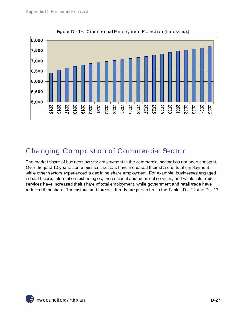
Appendix D: Economic Forecast
nwcouncil.org/7thplan D-27
Figure D - 19: Commercial Employment Projection (thousands)
Changing Composition of Commercial Sector The market share of business activity employment in the commercial sector has not been constant. Over the past 10 years, some business sectors have increased their share of total employment, while other sectors experienced a declining share employment. For example, businesses engaged in health care, information technologies, professional and technical services, and wholesale trade services have increased their share of total employment, while government and retail trade have reduced their share. The historic and forecast trends are presented in the Tables D – 12 and D – 13.

Appendix D: Economic Forecast
nwcouncil.org/7thplan D-28
Table D - 12: Number of employees in the commercial enterprises
1997 2007 2015 2035
Accommodation and Food Services 406 486 486 480 Administrative and Support Services 229 312 412 665 Arts, Entertainment, and Recreation 68 91 96 104 Educational Services 66 88 86 101 Federal Government 901 1,031 1,042 1,108 Finance and Insurance 169 207 210 209 Health Care and Social Assistance 457 606 660 807 Information 122 158 167 263 Management of Companies and Enterprises 60 74 73 84 Other Services (except Public Administration) 185 202 194 219 Professional, Scientific, and Technical Services 215 282 303 522 Real Estate and Rental and Leasing 94 110 111 120 Retail Trade 585 672 654 650 Transportation and Warehousing 164 179 185 224 Utilities 15 14 13 11 Wholesale Trade 231 255 259 361 Total Commercial Employment 3,969 4,767 4,952 5,930
Table D - 13: Percent Market Share of Employment
Market share Commercial Establishments 1997 2007 2015 2035 Accommodation and Food Services 10% 10% 10% 8% Administrative and Support Services 6% 7% 8% 11% Arts, Entertainment, and Recreation 2% 2% 2% 2% Educational Services 2% 2% 2% 2% Federal Government 23% 22% 21% 19% Finance and Insurance 4% 4% 4% 4% Health Care and Social Assistance 12% 13% 13% 14% Information 3% 3% 3% 4% Management of Companies and Enterprises 2% 2% 1% 1% Other Services (except Public Administration) 5% 4% 4% 4% Professional, Scientific, and Technical Services 5% 6% 6% 9% Real Estate and Rental and Leasing 2% 2% 2% 2% Retail Trade 15% 14% 13% 11% Transportation and Warehousing 4% 4% 4% 4% Utilities 0% 0% 0% 0% Wholesale Trade 6% 5% 5% 6%

Appendix D: Economic Forecast
nwcouncil.org/7thplan D-29
Figure D - 20: 2013 Stock of Commercial floor space by Business type (millions sqft)
Commercial Floor Space Additions Figure D – 20 shows the 2013 floor space by building activity type. The floor space stock in each year is the sum of new floor space additions and retirements from the floor space in that year.
The overall pattern of floor space additions for the commercial sector is presented in the Figure D - 21. A quick review of the historic data shows the cyclical nature of commercial floor space additions. The sharp increase in late 1980s is followed by a significant slowdown in the early 1990s. The late 1990s indicate a sharp increase in new construction activities. The 2000-2002 recession slowed construction activities. In 2005, another wave of commercial construction took place. Due to the long construction time for commercial activities, it would typically take a year or two for construction activities to reflect the economy.
The long-term forecast projects a slowdown in floor space additions, from 60 million square feet per year to about 40 to 50 million square feet. The forecast for future floor space additions do show a wide swing in construction activities in this sector. However, these swings in construction activity are not due to business cycles but rather due to changing demographics and changing in commercial trends.

Appendix D: Economic Forecast
nwcouncil.org/7thplan D-30
Figure D - 21: Total Commercial Floor Space Additions (Millions of SQFT)
The forecast for floor space additions for each state and the region is shown in the Table D - 14. The Council’s Seventh Power Plan forecasts about 950 million square feet of new floor space. A large portion of this will be in warehouse space, office space, hospitals, and elder care facilities.

Appendix D: Economic Forecast
nwcouncil.org/7thplan D-31
Table D - 14: 2015-2035 New Commercial Floor Space Additions (millions of sqf)
Idaho Montana Oregon Washington Region
Large Office 13.0 3.5 33.1 90.0 139.6 Medium Office 16.3 10.2 31.7 56.2 114.4 Small Office 4.0 2.8 8.8 14.5 30.1 Extra large Retail 2.5 2.4 8.6 12.1 25.6 Large Retail 1.2 1.2 3.7 4.4 10.4 Medium Retail 4.0 7.3 13.5 15.8 40.6 Small Retail 1.3 2.4 4.9 4.4 12.9 K-12 6.5 0.4 16.6 5.0 28.5 University 5.1 0.4 1.9 13.2 20.6 Warehouse 9.8 7.6 48.7 29.6 95.7 Supermarket 0.3 0.5 1.9 3.2 5.9 Mini Mart 0.1 0.2 1.1 1.1 2.4 Restaurant 0.8 1.8 3.1 5.7 11.5 Lodging 0.9 3.0 7.0 12.3 23.2 Hospital 9.7 4.0 5.6 23.5 42.9 Elder care facilities 2.6 3.6 21.7 27.0 54.9 Assembly 14.5 8.1 30.0 34.3 86.8 Other 33.2 15.6 103.4 49.9 202.2 Total 125.8 74.8 345.3 402.2 948.2
Patterns of Commercial Floor Space Additions
Commercial floor space additions typically show a cyclical pattern of overbuilding followed by high occupancy and demand for more space. This is especially true for the more speculative building types such as office or retail. A brief review of commercial floor space additions for 1987-2035 shows the different patterns of floor space additions for office, retail, warehouse, K-12 schools, and elder care facilities. An increase in office space additions, declining retail space requirements, substantial increases in new warehouse space, and declining additional K-12 school floor space requirements are forecast. Figures D – 22 through D-26 show the historical and Seventh Plan’s forecast for floor space additions for five major business types.
Office space requirements, shown in Figure D – 22, suggest a decline in new office space additions for 2012-2014, followed by a stable period from 2015-2019. Starting with 2020, the Council forecasts an escalation of commercial office construction activities.

Appendix D: Economic Forecast
nwcouncil.org/7thplan D-32
Figure D - 22: Pattern of Office Space Addition (millions of sqf)
As shown in Figure D – 23, the Seventh Plan forecast a decrease in retail floor space requirements. This results in a decline in new retail space additions over the forecast period. This decrease reflects slower population growth and the move to e-commerce. Retail space additions peaked in 2005-2006. In the 2015-2035 period, retail commercial floor space is forecast to average around 3 to 4 million square feet per year.
A decrease in retail space requirement is off-set by an increase in demand for warehouse space. This is shown in Figure D – 24. The increase in warehouse space reflects the expanding market for e-commerce. Available data from F.W.Dodge indicates that in 2012 there were no new warehouse additions.
Figure D - 23: Pattern of Retail Space Addition (millions sqf)

Appendix D: Economic Forecast
nwcouncil.org/7thplan D-33
Figure D - 24: Pattern of Warehouse Floor Space Additions (millions of sqf)
The demand for the schools and elder care are driven by the demographic changes facing the region. Population in the region is growing at a slower rate and a larger population is at retirement age. The pattern of floor space additions for K-12 schools shown in Figure D - 25 reflects the declining share of the population under 19 years old. Between 1985 and 2015, the regional population of this age group increased by about 800,000. But between 2015 and 2035, this population group is forecast to grow by about 450,000 people. Expected increase in this population cohort calls for increase in K-12 floors pace additions in post 2020 period. For period 2025 to 2035 floor space additions are stable at just below 2 million square feet per year, significantly below their historic levels.
Figure D - 25: Pattern of Floor Space Addition for K-12 Schools (million sqf)
The elderly population, 65 and older, is increasing from about one million in 1985 to about 2.6 million by 2015, and to over 3.8 million by 2035. As shown in Figure D – 26, this more than doubling of population is forecast to increase the demand for special elder care facilities. In the 2011 to 2018

Appendix D: Economic Forecast
nwcouncil.org/7thplan D-34
period, new floor space for these facilities is forecast to increase significantly to about 7 to 8 million square feet per year. After 2020, the forecast for new floor space drops is to drop to 4 to 5 million square feet per year.
Figure D - 26: Pattern of Floor Space Addition for Elder Care Facilities (million sqf)
Commercial Floor Space Stock Commercial floor space stock is projected to increase from 3.4 billion square feet in 2014 to about 4.3 billion square feet over the 2015 to 2035 period. The detailed projections by business activity type are shown in Table D – 15. As discussed above, sectors showing the greatest increase in floor space additions are large office, warehouse, and other health (elder care) facilities. Note that the warehouse floor space shown in Figure D-24 does not include self-storage facilities or warehouses associated with manufacturing facilities.
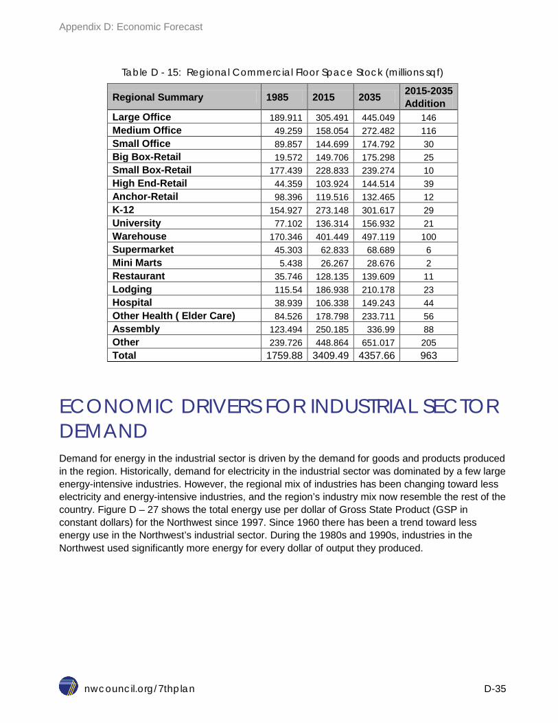
Appendix D: Economic Forecast
nwcouncil.org/7thplan D-35
Table D - 15: Regional Commercial Floor Space Stock (millions sqf)
Regional Summary 1985 2015 2035 2015-2035 Addition
Large Office 189.911 305.491 445.049 146 Medium Office 49.259 158.054 272.482 116 Small Office 89.857 144.699 174.792 30 Big Box-Retail 19.572 149.706 175.298 25 Small Box-Retail 177.439 228.833 239.274 10 High End-Retail 44.359 103.924 144.514 39 Anchor-Retail 98.396 119.516 132.465 12 K-12 154.927 273.148 301.617 29 University 77.102 136.314 156.932 21 Warehouse 170.346 401.449 497.119 100 Supermarket 45.303 62.833 68.689 6 Mini Marts 5.438 26.267 28.676 2 Restaurant 35.746 128.135 139.609 11 Lodging 115.54 186.938 210.178 23 Hospital 38.939 106.338 149.243 44 Other Health ( Elder Care) 84.526 178.798 233.711 56 Assembly 123.494 250.185 336.99 88 Other 239.726 448.864 651.017 205 Total 1759.88 3409.49 4357.66 963
ECONOMIC DRIVERS FOR INDUSTRIAL SECTOR DEMAND Demand for energy in the industrial sector is driven by the demand for goods and products produced in the region. Historically, demand for electricity in the industrial sector was dominated by a few large energy-intensive industries. However, the regional mix of industries has been changing toward less electricity and energy-intensive industries, and the region’s industry mix now resemble the rest of the country. Figure D – 27 shows the total energy use per dollar of Gross State Product (GSP in constant dollars) for the Northwest since 1997. Since 1960 there has been a trend toward less energy use in the Northwest’s industrial sector. During the 1980s and 1990s, industries in the Northwest used significantly more energy for every dollar of output they produced.

Appendix D: Economic Forecast
nwcouncil.org/7thplan D-36
Figure D - 27: Change in Regional Energy Intensity
2012 $GSP/Energy consumption Indexed to 1997 levels
Projected Employment Growth The demand forecast model tracks distinct industries. In the Seventh Plan, the Council used the growth in employment and changes in productivity for each industry to forecast future electricity demand. Productivity was measured in terms of dollars of output per employee times hours worked. Industrial employment has been on the decline, but the Seventh Plan forecast is for a projected slight increase in the 2015-2020 period, stable in the 2020-2030 period, followed by a slight decrease from 2030-2035. Figure D - 28 shows the number of industrial employees for selected historic and forecast periods. Industrial employment peaked at about 650,000 in 2000, but it declined significantly during the 2000-2010 period. By 2010 it was down to about 500,000 employees. By 2035 employment in manufacturing is expected to reach to about 570,000 employees.
0
50
100
150
200
250
Idaho
Montana
Oregon
Washington

Appendix D: Economic Forecast
nwcouncil.org/7thplan D-37
Figure D - 28: Employment in Manufacturing Sectors (1000s)
The demand for energy consumed in each industry is forecast using the estimated growth in the product output in that industry. Output in each industry is forecast starting with the projected output from Global Insight. The output level projections are then modified, based on input from Demand Forecast Advisory Committee.
Industrial Output State level industrial output is forecasted using Global Insight’s product Business Markets Insight. The 4 to 6 digit NAICS code forecasts were used to identify fast growing industries. Growth in output of major industries in the Northwest and nation reflect changes in productivity observed over the past few decades. The following three figures show the change in labor productivity in the United States. Decline in productivity since the start of the recession has been significant, the growth rate dropping by a full percentage point. Drop in manufacturing sector has been even more pronounced, dropping by 2 full percentage points since start of the 2007 recession.
0
100
200
300
400
500
600
700
800
WA OR MT ID

Appendix D: Economic Forecast
nwcouncil.org/7thplan D-38
Figure D - 29: Average Annual Percent Change in non-farm Business sector (National Data)
Figure D - 30: Average Annual Percent Change in Manufacturing sector (National Data)
0
0.5
1
1.5
2
2.5
3
1947-1973
1973-1979
1979-1990
1990-2000
2000-2007
2007-2014
0 0.5
1 1.5
2 2.5
3 3.5
4 4.5
1987-1990 1990-2000 2000-2007 2007-2014

Appendix D: Economic Forecast
nwcouncil.org/7thplan D-39
Figure D - 31: National improvement in Labor Productivity 1987 and 2012 indexed to 2000
Labor productivity is measured as dollar value of output per one hour of labor.
The composition of industrial output is also forecast to change. Manufacturing facilities producing food, rubber, paper, transportation, and chemicals are forecasted to grow while machines and computer (hardware) and lumber are projected to decline further.
Table D – 16 shows the dollar value of industrial output, which drives demand for this sector.
0 50 100 150 200
311 - Food manufacturing
312 - Beverages and tobacco products
321 - Wood products
322 - Paper and paper products
323 - Printing and related support activities
324 - Petroleum and coal products
325 - Chemicals
326 - Plastics and rubber products
327 - Nonmetallic mineral products
331 - Primary metals
332 - Fabricated metal products
333 - Machinery
334 - Computer and electronic products
335 - Electrical equipment and appliances
336 - Transportation equipment
2002=100
2012 1987

Appendix D: Economic Forecast
nwcouncil.org/7thplan D-40
Table D - 16: Regional Industrial Output (billions of $2012)
1985 2007 2015 2035 1985-2015 AAGR
2015-2035 AAGR
Food & Tobacco 8.5908 13.7142 15.9948 27.4651 2% 3% Textiles 0.2022 0.5799 0.7792 0.8842 5% 1% Apparel 0.6289 0.3308 0.2227 0.1838 -3% -1% Lumber 19.0112 9.5444 9.2299 5.2684 -2% -3% Furniture 0.5779 2.7812 1.5556 3.1815 3% 4% Paper 5.4951 6.2486 4.8832 8.697 0% 3% Printing 3.7553 1.6765 1.128 1.4294 -4% 1% Chemicals 0.9843 3.7532 4.8415 12.9812 5% 5% Petroleum Products 3.2162 5.3746 6.1474 9.3096 2% 2% Rubber 0.9495 2.5096 2.4278 4.9968 3% 4% Leather 0.0796 0.0796 0.0971 0.0796 1% -1% Stone, Clay, etc. 1.409 3.4592 3.0906 6.1438 3% 3% Fabricated Metals 1.9297 3.2182 3.6902 3.1243 2% -1% Machines & Computer 3.0018 7.1634 7.7106 6.851 3% -1% Electric Equipment 8.8317 8.9195 9.8285 9.671 0% 0% Transport Equipment 2.7853 1.2824 1.2669 1.4886 -3% 1% Other Manufacturing 23.2831 28.9599 29.0039 36.1335 1% 1% Agriculture 0.9822 3.2713 4.0204 8.9499 5% 4% Two other sectors are included in the industrial demand for electricity: custom data centers and Direct Service Industries. The demand for electricity from direct service industries is based on projections provided in the BPA White Book 2012 and data from the Chelan Public Utility District. Detailed discussions on the methodology and forecast for both custom data centers and direct service industries are in the demand forecast Appendix E.
ECONOMIC DRIVERS FOR OTHER SECTORS Irrigation Demand for electricity for irrigation is linked to agricultural output. A forecast of agricultural output in constant dollars is provided in the Table D -16. Agricultural output in the region is forecast to increase from about $4 billion in 2015 to about $9 billion by 2035.
Transportation In the current analysis, demand for electricity in the transportation sector is not limited to public transportation, such as the electric rail and bus transportation systems in Portland and Seattle; it also includes electric demand for powering plug-in hybrid and fully electric vehicles. The key
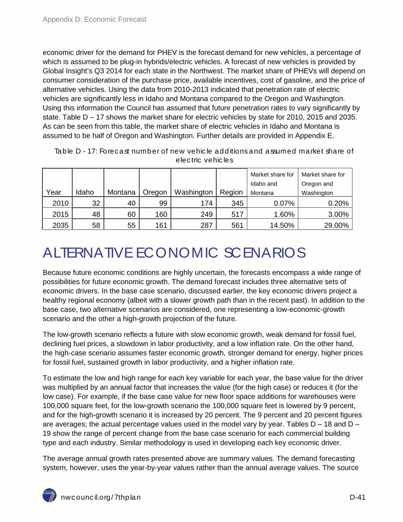
Appendix D: Economic Forecast
nwcouncil.org/7thplan D-41
economic driver for the demand for PHEV is the forecast demand for new vehicles, a percentage of which is assumed to be plug-in hybrids/electric vehicles. A forecast of new vehicles is provided by Global Insight’s Q3 2014 for each state in the Northwest. The market share of PHEVs will depend on consumer consideration of the purchase price, available incentives, cost of gasoline, and the price of alternative vehicles. Using the data from 2010-2013 indicated that penetration rate of electric vehicles are significantly less in Idaho and Montana compared to the Oregon and Washington. Using this information the Council has assumed that future penetration rates to vary significantly by state. Table D – 17 shows the market share for electric vehicles by state for 2010, 2015 and 2035. As can be seen from this table, the market share of electric vehicles in Idaho and Montana is assumed to be half of Oregon and Washington. Further details are provided in Appendix E.
Table D - 17: Forecast number of new vehicle additions and assumed market share of electric vehicles
Year Idaho Montana Oregon Washington Region
Market share for Idaho and Montana
Market share for Oregon and Washington
2010 32 40 99 174 345 0.07% 0.20% 2015 48 60 160 249 517 1.60% 3.00% 2035 58 55 161 287 561 14.50% 29.00%
ALTERNATIVE ECONOMIC SCENARIOS Because future economic conditions are highly uncertain, the forecasts encompass a wide range of possibilities for future economic growth. The demand forecast includes three alternative sets of economic drivers. In the base case scenario, discussed earlier, the key economic drivers project a healthy regional economy (albeit with a slower growth path than in the recent past). In addition to the base case, two alternative scenarios are considered, one representing a low-economic-growth scenario and the other a high-growth projection of the future.
The low-growth scenario reflects a future with slow economic growth, weak demand for fossil fuel, declining fuel prices, a slowdown in labor productivity, and a low inflation rate. On the other hand, the high-case scenario assumes faster economic growth, stronger demand for energy, higher prices for fossil fuel, sustained growth in labor productivity, and a higher inflation rate.
To estimate the low and high range for each key variable for each year, the base value for the driver was multiplied by an annual factor that increases the value (for the high case) or reduces it (for the low case). For example, if the base case value for new floor space additions for warehouses were 100,000 square feet, for the low-growth scenario the 100,000 square feet is lowered by 9 percent, and for the high-growth scenario it is increased by 20 percent. The 9 percent and 20 percent figures are averages; the actual percentage values used in the model vary by year. Tables D – 18 and D – 19 show the range of percent change from the base case scenario for each commercial building type and each industry. Similar methodology is used in developing each key economic driver.
The average annual growth rates presented above are summary values. The demand forecasting system, however, uses the year-by-year values rather than the annual average values. The source

Appendix D: Economic Forecast
nwcouncil.org/7thplan D-42
of the range forecast used in the Seventh Plan, is Global Insight’s long-term national forecast, Q4 2014.
Tables D – 18 and D – 19 also show the annual growth rate for the historic and forecast period for the region. In general, the key economic drivers reflect a slowdown in economic growth for 2015-2035 compared to historic growth rates.

Appendix D: Economic Forecast
nwcouncil.org/7thplan D-43
Table D - 18: Historic and Forecast of Annual Growth Rate by Sector
Actual Base Low High 1985-2012 2013-2035 2013-2035 2013-2035 Single Family - Million Sq Ft 1.8% 1.10% 0.72% 1.52% Multi Family - Million Sq Ft 2.8% 2.15% 1.82% 2.76% Other Family - Million Sq Ft 2.7% 0.34% 0.23% 0.57% Large Office - Million Sq Ft 1.8% 1.99% 1.81% 2.22% Medium Office - Million Sq Ft 4.4% 2.91% 2.74% 3.15% Small Office - Million Sq Ft 1.8% 0.97% 0.80% 1.21% Big Box-Retail - Million Sq Ft 7.8% 0.80% 0.61% 1.03% Small Box-Retail - Million Sq Ft 0.9% 0.22% 0.03% 0.45% High End-Retail - Million Sq Ft 3.2% 1.68% 1.49% 1.92% Anchor-Retail - Million Sq Ft 0.7% 0.51% 0.32% 0.75% K-12 - Million Sq Ft 2.1% 0.47% 0.20% 0.72% University - Million Sq Ft 2.1% 0.69% 0.42% 0.94% Warehouse - Million Sq Ft 3.2% 1.15% 0.78% 1.38% Supermarket - Million Sq Ft 1.2% 0.50% 0.30% 0.73% Mini Mart - Million Sq Ft 6.0% 0.47% 0.27% 0.70% Restaurant - Million Sq Ft 4.8% 0.46% 0.24% 0.69% Lodging - Million Sq Ft 1.8% 0.65% 0.43% 0.87% Hospital - Million Sq Ft 3.8% 1.83% 1.57% 2.07% Other Health - Million Sq Ft 2.8% 1.37% 1.12% 1.62% Assembly - Million Sq Ft 2.6% 1.62% 1.38% 1.85% Other - Million Sq Ft 2.4% 1.89% 1.51% 2.12% Food & Tobacco - 2012 B$ 2.3% 2.66% 2.35% 2.79% Textiles - 2012 B$ 5.1% 0.77% 0.31% 0.86% Apparel - 2012 B$ -3.8% -0.99% -1.35% -0.85% Lumber - 2012 B$ -2.6% -1.93% -2.19% -1.79% Furniture - 2012 B$ 3.7% 3.48% 3.37% 3.67% Paper - 2012 B$ -0.4% 2.83% 2.59% 2.97% Printing - 2012 B$ -4.4% 1.07% 0.84% 1.20% Chemicals - 2012 B$ 6.1% 5.11% 4.91% 5.28% Petroleum Products - 2012 B$ 2.4% 2.11% 1.91% 2.26% Rubber - 2012 B$ 3.5% 3.62% 3.45% 3.79% Leather - 2012 B$ 0.7% -1.21% -1.58% -1.07% Stone, Clay, etc. - 2012 B$ 3.0% 3.75% 3.47% 3.90% Other Primary Metals - 2012 B$ 2.4% -0.50% -0.73% -0.35% Fabricated Metals - 2012 B$ 3.6% -0.40% -0.57% -0.25% Machines & Computer - 2012 B$ 0.4% 0.21% -0.16% 0.37% Electric Equipment - 2012 B$ -2.9% 0.90% 0.75% 1.06% Transport Equipment - 2012 B$ 0.8% 0.96% 0.85% 1.14% Other Manufacturing - 2012 B$ 5.4% 3.95% 3.82% 4.14% Agriculture - 2012 B$ 0.4% 1.15% 0.63% 1.88%

Appendix D: Economic Forecast
nwcouncil.org/7thplan D-44
Summary range of annual average growth rates by sector are in the table below.
Table D - 19: Forecast of Range of Annual Growth Rate by Sector
Base case High case Low case
Residential Units 1.18% 2.0% 0.08%
Commercial Floor space 1.11% 2.1% 0.67%
Industrial output 1.56% 2.4% 0.95%
Agricultural output 0.81% 2.0% 0.26%
Additional Details: A companion Excel workbook containing details on the economic drivers is available from Council’s website: http://www.nwcouncil.org/energy/powerplan/7/technical

Seventh Northwest Conservation and Electric Power Plan
nwcouncil.org/7thplan E-1
APPENDIX E: DEMAND FORECAST
Contents Energy Demand ................................................................................................................................ 5
Background ................................................................................................................................... 5 Loads versus Demand ............................................................................................................... 7
Demand Forecast Methodology ..................................................................................................... 7 Demand Forecasting Model ....................................................................................................... 8
Load Forecast .............................................................................................................................. 10 Sector Level forecast ............................................................................................................... 12
Residential Sector Load ............................................................................................................... 12 History ...................................................................................................................................... 12 Residential Load Forecast ........................................................................................................ 16
Commercial Sector Load ............................................................................................................. 17 History ...................................................................................................................................... 17 Commercial Load Forecast ...................................................................................................... 18 Embedded Data Center Loads ................................................................................................. 19 Non-DSI Industrial Sector Loads .............................................................................................. 22 Non-DSI Industrial Load Forecast ............................................................................................ 23 Custom Data Centers ............................................................................................................... 24 Direct Service Industries .......................................................................................................... 25 Irrigation ................................................................................................................................... 26 Indoor Agriculture/Indoor Cannabis Production ........................................................................ 27 Transportation .......................................................................................................................... 28
Historical and Forecast of Loads by State .................................................................................... 29 Monthly Pattern of Load ............................................................................................................... 32
Regional Peak Load ........................................................................................................................ 33 Seasonal Variation in Load .......................................................................................................... 34
Average, Peak, and Off-peak Loads ......................................................................................... 34 Loads versus Demand/Sales.................................................................................................... 35 Sector Level Demand/Sales ..................................................................................................... 36
Distributed Solar Photovoltaics .................................................................................................... 38 Calculations for Alternative Load Forecast Concepts ................................................................... 39
Electricity Demand Growth in the West ........................................................................................... 44 Special Forecast Topics .................................................................................................................. 47
Estimating Electricity Demand in Data Centers ............................................................................ 47 Background on Trends in Data Center Load ............................................................................ 47 What is a Data Center? ............................................................................................................ 47
Load Forecast for Data Centers in the Region ............................................................................. 49

Appendix E: Demand Forecast
nwcouncil.org/7thplan E-2
Embedded Data Centers .......................................................................................................... 49 Enterprise and Cloud Data Centers .......................................................................................... 51
Regional Data Center Energy Consumption 2014-2035 ............................................................... 52 Future Trends for Plug-in Hybrid or all Electric Vehicles (EV) ...................................................... 54
Background .............................................................................................................................. 54 Potential Effects on Electricity Demand .................................................................................... 56
Estimating Electricity Demand in Indoor Cannabis Production ..................................................... 59 Background on Cannabis Production and Recent Changes in Cannabis Legislation ................ 59 Baseline for Indoor Production ................................................................................................. 59 Load Forecast for Indoor Cannabis Production ........................................................................ 60
List of Figures and Tables
Figure E - 1: Total and Non-DSI Regional Electricity Sales (AMW) ................................................... 5 Table E - 1: Total and Non-DSI Regional Electricity Sales ................................................................. 6 Figure E - 2: Trends in Electricity Intensity Per Capita 1960-2012 (index to 1980) ............................. 6 Figure E - 3: Overview of Council’s Long Term Forecasting Model ................................................... 9 Figure E - 4: Range of Load forecast – prior to conservation (aMW) ............................................... 11 Figure E - 5: Range of Peak Load forecast – prior to conservation (aMW) ..................................... 11 Table E - 2: Sector level Range of Load Forecast (Energy aMW) .................................................... 12 Figure E - 6: Change in Residential Per Capita Consumption ......................................................... 13 (weather adjusted) ........................................................................................................................... 13 Figure E - 7: Residential per Household Consumption (MWH/household) ....................................... 13 Table E - 3: Range of load forecast by enduse in Residential sector (aMW).................................... 14 Figure E - 8: Change in Residential per Household Consumption ................................................... 15 Medium Growth Scenario ................................................................................................................ 15 Table E - 4: Estimated Impact of federal standards by sector (aMW)-Medium Scenario .................. 16 Figure E - 9: Historic and Range of Forecast for Residential Load (aMW)* ..................................... 16 Figure E - 10: Electricity Intensity in the Commercial Sector (kWh/SQF) ......................................... 17 Figure E - 11: Electricity Intensity in the Commercial Sector (MWh/customer) ................................. 18 Table E - 5: Enduse Level Forecast of Loads in Commercial Sector (aMW) .................................... 18 Figure E - 12: Forecast Commercial Electricity Loads (aMW) .......................................................... 19 Table E - 6: 2013 Estimated Use by Application and Data Center Types (aMW) ............................. 20 Figure E - 13: Possible range of Embedded Data Center Loads with different technology paths (aMW) ............................................................................................................................................. 21 Figure E - 14: Forecast Embedded Data Center Loads (aMW)........................................................ 21 Figure E - 15: Forecast Industrial Loads by Industry 2015 (aMW) ................................................... 22 Table E - 7: Changing Electric Intensity of Industries in the Northwest ............................................ 23 Figure E - 16: Electricity Intensity in the Industrial Sector ................................................................ 23 Figure E - 17: Historical and Forecast Non-DSI Industrial* Load ..................................................... 24 Figure E - 18: Projected Load from Custom Data Centers ............................................................... 25 Figure E - 19: Historical and Forecast DSI Electricity Loads ............................................................ 26 Figure E - 20: Historical and Forecast Irrigation Loads .................................................................... 27 Figure E - 21: Indoor Agriculture/Cannabis Load Forecast .............................................................. 28 Figure E - 22: Forecast of Load from PHEV/Electric Vehicles (aMW) .............................................. 29

Appendix E: Demand Forecast
nwcouncil.org/7thplan E-3
Table E - 8: Historic and forecasted range of growth in state loads ................................................. 30 Figure E - 23: Historic and Forecast Electric Load for State of Idaho ............................................... 30 Figure E - 24: Historic and Forecast Electric Load for Western Montana ......................................... 31 Figure E - 25: Historic and Forecast Electric load for State of Oregon ............................................. 31 Figure E - 26: Historic and Forecast Electric Load for State of Washington ..................................... 32 Figure E - 27: Monthly Pattern of Demand for Electricity ................................................................. 33 Table E - 9: Monthly Pattern of Demand for Electricity .................................................................... 33 Figure E - 28: Range of Variation in Load ....................................................................................... 34 Figure E - 29: Historical and Forecast Range of Winter Peak Loads ............................................... 35 Figure E - 30: Historical and Forecast Range of Summer Peak Loads ............................................ 35 Figure E - 31: Comparison of Historical and Forecast Loads and Demand/Sales ............................ 36 Table E - 10: Forecast Range of Growth in Demand/Sales (aMW) .................................................. 37 Figure E - 32: Historic and Forecast Range of Annual Energy Generation from Distributed PV ....... 38 Figure E - 33: Historic and Forecast Range of Summer Peak Generation from Distributed PV........ 39 Table E - 11: Range of Alternative Load Forecasts (as measured at the point of generation) .......... 40 Figure E - 34: Range Forecast for Price-Effect – Energy ................................................................. 41 Figure E - 35: Range Forecast for Frozen-Efficiency – Energy ........................................................ 41 Figure E - 36: Range Forecast for Sales – Energy ......................................................................... 42 Figure E - 37: Range Forecast Price-effect Winter Peak ................................................................. 42 Figure E - 38: Range Forecast Frozen-Efficiency – Winter Peak ..................................................... 42 Figure E - 39: Range Forecast Sales – Winter Peak ....................................................................... 43 Figure E - 40: Range Forecast Price-Effect – Summer Peak ........................................................... 43 Figure E - 41: Range Forecast Frozen-Efficiency – Summer Peak .................................................. 43 Table E - 12 - Naming Convention for Aurora Areas ........................................................................ 45 Figure E - 43: 2013 and 2035 Load by AURORA Areas outside NW ............................................... 46 Figure E - 44: 2015-2035 Average Annual Growth Rate for Loads Outside NW .............................. 46 Figure E - 45: Projected Peak Load by AURORA Area Outside Northwest..................................... 47 Table E - 13: Characteristics of Data Centers .................................................................................. 48 Figure E - 46: Monthly Average & Peak Demand for Power from Six Large Data Centers in the NW ........................................................................................................................................................ 49 Table E - 14: Count of Embedded Data Centers in Northwest ......................................................... 49 Table E - 15: Estimated current data center load by data center type and enduse (aMW) ............... 50 Figure E - 47: Estimates for Energy Consumption in 2014 for all Data Centers in the Region ......... 52 Figure E - 48: NWPCC Regional Data Center Energy Use by Space Type under Business as Usual Scenario .......................................................................................................................................... 52 Figure E - 49: Possible range of loads for embedded data centers .................................................. 53 Figure E - 50: count of EV and PHEV vehicles Nationwide .............................................................. 54 Table E - 16: Allocation of Vehicles by state and type ..................................................................... 55 Figure E – 51: Electric Vehicles Registered by County in Washington State ................................... 55 Figure E – 52: Electric Vehicles Registered by County in Oregon State .......................................... 56 Figure E – 53 Load Profile for Electric Vehicle Charging ................................................................. 57 Table E - 17: Impact of Electric Vehicle on Northwest Regional Load.............................................. 58 Figure E - 54: Preliminary Estimates for Cannabis in Metric Tons by State ..................................... 61 Table E - 18: kWh/Kg by Production Option and % of Producers who chose to Produce in Each Option ............................................................................................................................................. 62 Table E - 19: Preliminary Estimate for Energy Used in Indoor Production Derived from Tier Size ... 64

Appendix E: Demand Forecast
nwcouncil.org/7thplan E-4
Throughout this write-up load forecast is presented in form of a low and high range. This is done to reinforce the fact that future is uncertain. Council’s planning process does not use a single deterministic future to drive the analysis. The stochastic variation introduced in the Regional Portfolio Model tests a wide range of future uncertainties in load, fuel prices etc.
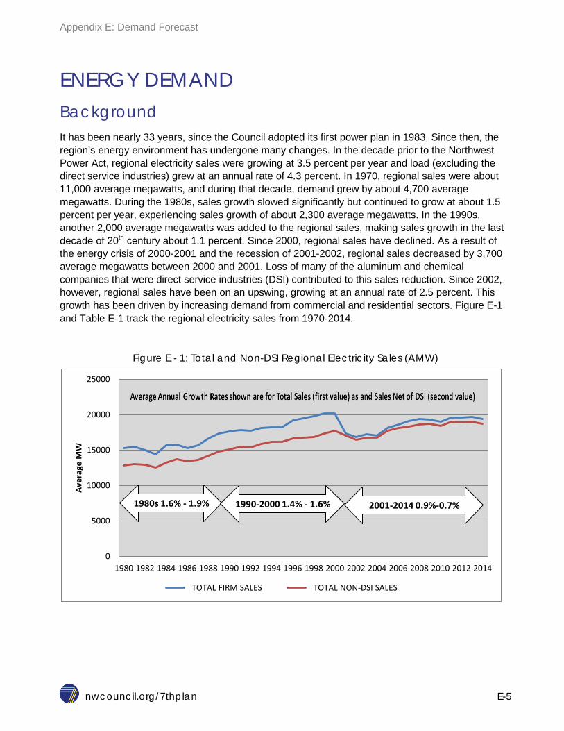
Appendix E: Demand Forecast
nwcouncil.org/7thplan E-5
ENERGY DEMAND Background It has been nearly 33 years, since the Council adopted its first power plan in 1983. Since then, the region’s energy environment has undergone many changes. In the decade prior to the Northwest Power Act, regional electricity sales were growing at 3.5 percent per year and load (excluding the direct service industries) grew at an annual rate of 4.3 percent. In 1970, regional sales were about 11,000 average megawatts, and during that decade, demand grew by about 4,700 average megawatts. During the 1980s, sales growth slowed significantly but continued to grow at about 1.5 percent per year, experiencing sales growth of about 2,300 average megawatts. In the 1990s, another 2,000 average megawatts was added to the regional sales, making sales growth in the last decade of 20th century about 1.1 percent. Since 2000, regional sales have declined. As a result of the energy crisis of 2000-2001 and the recession of 2001-2002, regional sales decreased by 3,700 average megawatts between 2000 and 2001. Loss of many of the aluminum and chemical companies that were direct service industries (DSI) contributed to this sales reduction. Since 2002, however, regional sales have been on an upswing, growing at an annual rate of 2.5 percent. This growth has been driven by increasing demand from commercial and residential sectors. Figure E-1 and Table E-1 track the regional electricity sales from 1970-2014.
Figure E - 1: Total and Non-DSI Regional Electricity Sales (AMW)
0
5000
10000
15000
20000
25000
1980 1982 1984 1986 1988 1990 1992 1994 1996 1998 2000 2002 2004 2006 2008 2010 2012 2014
Aver
age
MW
TOTAL FIRM SALES TOTAL NON-DSI SALES
1980s 1.6% - 1.9% 1990-2000 1.4% - 1.6% 2001-2014 0.9%-0.7%

Appendix E: Demand Forecast
nwcouncil.org/7thplan E-6
Table E - 1: Total and Non-DSI Regional Electricity Sales
Annual Growth Total Sales Non DSI
1970-1979 4.1% 5.2%
1980-1989 1.5% 1.7%
1990-1999 1.1% 1.5%
2000-2007 -0.8% 0.5%
2007-2014 0.3% 0.3%
The dramatic decrease in the growth of electricity demand shown in Table E-1 was not due to a slowdown in economic growth in the region. The region added more population and more jobs between 1980 and 2000 than it did between 1960 and 1980. The decrease in demand was the result of a move to less energy-intensive activities and greater energy efficiency. As shown in Figure E-2, electric intensity in terms of use per capita increased between 1980 and 1990, but has been declining since 1990. This shift reflects industry changes, increasing electricity prices, and regional and national conservation efforts.
Figure E - 2: Trends in Electricity Intensity Per Capita 1960-2012 (index to 1980)
In the past two decades, the region’s population has grown from roughly 9 million in 1985 to more than almost 13.5 million by 2012. Regional population growth, consistent with the national trends, is expected to slow down from the historic 1.5 percent to about 0.9 percent per year in the forecast period.
0
0.2
0.4
0.6
0.8
1
1.2
1.4
1.6
1960
19
62
1964
19
66
1968
19
70
1972
19
74
1976
19
78
1980
19
82
1984
19
86
1988
19
90
1992
19
94
1996
19
98
2000
20
02
2004
20
06
2008
20
10
2012
PNW
US

Appendix E: Demand Forecast
nwcouncil.org/7thplan E-7
Loads versus Demand
In this document to terms are used to describe the amount of electricity used in the region. Demand (or sales) is the measure of electricity use at the customer meter. Load is the measure of electricity use at generator. Load represents the total amount of electricity generation needed to supply the demand for electricity at the point of use. The difference between electricity sales/demand and load are the losses that occur on the region’s transmission and distribution systems.
The Council’s Demand Forecasting System (DFS) produces three different forecasts. These forecasts are labeled Price-effect, Frozen-efficiency and Sales forecast. Price-effect forecast captures the impact of price and non-price effects on demand for electricity. The Frozen-efficiency forecast measures future demand based on the assumption that the efficiency of devices using electricity are kept constant (i.e., “frozen”) throughout the planning horizon. For the Seventh Power Plan, this was their efficiency level in 2015. The frozen efficiency forecast is used in Council’s planning process to permit the treatment of energy efficiency as a resource in the Regional Portfolio Model (RPM). The Sales forecast nets out the amount of cost-effective conservation and demand response resources developed in the RPM from Frozen-efficiency demand forecast. This is done to simulate how consumers will respond to lower bills resulting from the installation of conservation measures. Note that for each one of these forecasts the Council estimates both the regional electric load at the generator and electricity sales at the consumer’s meter.
Demand Forecast Methodology When the Council was formed, growth in electricity demand was considered the key issue for planning. The region was beginning to see a slowing of its historically rapid growth of electricity use, and it began to question the need for several proposed nuclear and coal generating plants. To respond to these changes, it was important that the Council’s demand forecasting system (DFS) be able to determine the causes of changing demand growth and the extent and composition of future demand trends. Simple historical trends, used in the past, were no longer reliable indicators of future demand.
In addition, the Northwest Power Act requires the Council to consider conservation a resource, and to evaluate it along with new generation as a source for meeting future demand for electricity. As a result, the DFS analysis also needed to support a detailed evaluation of energy efficiency improvements and their effects on electricity demand.
Rather than identifying trends in aggregate or electricity consumption by sector, the Council developed a forecasting system that incorporates end-use details of each consuming sector (residential, commercial, industrial). Forecasting with these models requires detailed separate economic forecasts for all the sectors represented in the demand models. The models also require forecasts of demographic trends, electricity prices, and fuel prices.
As Western electricity systems became more integrated through deregulated wholesale markets, and as capacity issues began to emerge, it became clear that the Council needed to understand the pattern of electricity demand over seasons, months, and hours of the day. The load shape forecasting system (LSFS) was developed to do this. The model identifies the equipment that is contributing to demand and how much electricity it is using during each hour of the day across all

Appendix E: Demand Forecast
nwcouncil.org/7thplan E-8
hours of the year. All of these individual end use patterns are aggregated up to represent the total power systems hourly shape of electricity demand.
Although the Northwest Power Act still requires a 20-year forecast of demand, changes in the electricity industry have meant a greater focus on the short-term energy landscape. When the Council developed its first several plans, large-scale nuclear and coal plants were the resources options available. These resources took 8 to 12 years to site, license and construct. Now, natural gas-fired combustion turbines, solar PV or wind generation which take 2 to 4 years plan and develop are the principal resources being considered for development. As a result the need to analyze the uncertainty surrounding long-term load growth is less of an issue than it was in the past.
One of the most significant issues facing the region’s power system today is that the pattern of electricity demand and the resource mix used to meet that demand have changed. The question is not only if we have energy to meet annual demand, but whether we have adequate capacity to meet times of peak demand. The Pacific Northwest now more closely resembles the rest of the West, which has always been capacity constrained. In response, the Seventh Power Plan is focuses on both capacity and energy demand forecast.
Additionally, the region is no longer independent of the entire Western U.S. electricity market. Electricity prices and the adequacy of supply are now determined by West-wide electricity conditions. The Council uses the AURORAxmp®
electricity market model, which requires
assumptions about demand growth for all areas of the Western-integrated electricity grid.
Given all these changes, the Council demand forecast system must be able to analyze short-term, temporal patterns of demand over expanded geographic areas. In addition, the demand forecasting system must address the effect of energy-efficiency improvements on both annual and hourly use of electricity.
Demand Forecasting Model
The 2000-2001 Western energy crisis created renewed interest in demand forecasting and the Northwest’s changing resource mix has created a particular concern about the ability to supply peak capacity.1 In order to forecast these peaks, the Council relies on end-use forecasting models. For its Sixth Power Plan, the Council selected a new end-use forecasting and policy analysis tool, the Energy 2020 model. The Council’s Seventh Power Plan demand forecasting system (DFS) also uses the Energy 2020 model to generate forecasts for electricity, natural gas, and other fuel.
The Energy 2020 model is fully integrated and includes all fuels, sectors, and multiple end-use demand. The Council uses Energy 2020 to forecast annual and peak sales and loads for electricity as well as for other fuels. The following flow-chart provides an overview of the Energy 2020 model.
1 See Chapter 11 for a discussion of the regional load and resource balance.

Appendix E: Demand Forecast
nwcouncil.org/7thplan E-9
Figure E - 3: Overview of Council’s Long Term Forecasting Model
The Energy 2020 is calibrated to total demand for electricity, natural gas, oil, and a range of other fuel. The data for calibration is obtained from the Energy Information Administration’s State Energy Demand System (SEDS). Annual consumption data for each sector and state is available for years 1960-2012.
The basic version of Energy 2020 was expanded to meet the needs of the Council’s conservation resource planning process. This primarily required increasing the number of end-uses modeled. In the residential sector, the energy use of three building types, four different space-heating technologies, and two different space-cooling technologies, four different water heating types and sizes are now individually forecast. For the Seventh Power Plan, new end-uses were added, such as information, communication, and entertainment (ICE) devices, which are beginning to represent a growing share of electricity consumption in homes. Technology trade-off curves for each of these end-uses were updated with new cost and efficiency data. In total, demand for electricity is forecast for 12 individual end-uses in the residential sector.
Demand
Prices
ENERGY 2020
Sector Demand
Residential
Commercial
Industrial
Agricultural
Transportation
SUPPLY
Electric Utility
Gas Supply
Oil Supply
Coal Supply
Economic Drivers
Population
Number of Residences
Commercial sector floor space
Industrial Outputs
Agricultural output
Aggregate DEMAND
4 states and region
Electricity
Gas
Oil
Coal

Appendix E: Demand Forecast
nwcouncil.org/7thplan E-10
In the commercial sector, the Energy 2020 model was expanded to forecast energy demand for 18 different commercial building types for the Seventh Power Plan. A new forecast of commercial floor space was developed and was used for the conservation resource assessment.
For the Seventh Power Plan, the industrial sector of the Energy 2020 model was updated with new regional energy consumption data. The work on the industrial sector is ongoing and the results of a recent analysis on industrial demand for electricity were added to the demand forecast.
The load shape forecasting system was updated with the best available data on end-use load shapes. Specifically, new data from the recent Residential Building Stock Assessment completed by the Northwest Energy Efficiency Alliance (NEEA) was used.2
Load Forecast The Council’s Seventh Power Plan forecast electricity load to grow from about 19,400 average megawatts in 2012 to between 22,600 to 25,600 average megawatts by 2035. The average annual rate of growth over the 20-year planning period (2015-2035) is about 0.5 to 1 percent per year. This level of growth does not include expected load reductions from conservation. This rate of growth is lower than Council’s reference case for the Sixth Power Plan growth rate, which was projected to grow by between 0.8 and 1.7 percent per year from 2010 to 2030. The projected load growth for the Seventh Power Plan is between the low and medium case for the Sixth Power Plan. Two factors contribute to slower than anticipated load growth. The first is the impact of a prolonged recession. The second is the achievement of higher levels of energy efficiency from both programmatic and non-programmatic sources.
Regional electricity loads are forecast to grow, absent any future conservation, by between 1800 average megawatts in the low case and 4600 average megawatts by 2035, an average annual increase of about 90-220 average megawatts. The projected growth reflects increased electricity use by the residential and commercial and industrial sectors, and introduction of some new uses of electricity, including electric vehicles and indoor agriculture. Operating in the opposite direction, to reduce the pace of regional load growth are over 35 federal appliance and equipments standards that have been updated or established since 2010. Figure E - 4 shows the historical regional electricity load and the range of future load growth forecast for the Seventh Power Plan.
Lower electricity and natural gas prices have had a significant impact on the region’s industrial makeup. As a result of the energy crisis during 2000-2001 and the recession of 2001-2002, the region lost about 3,500 average megawatts of industrial load, which has not returned.
2 http://neea.org/resource-center/regional-data-resources/residential-building-stock-assessment

Appendix E: Demand Forecast
nwcouncil.org/7thplan E-11
Figure E - 4: Range of Load forecast – prior to conservation (aMW)
Impact of weather is reflected in regional single hour peaks. The forecast for the growth in peaks, under normal weather conditions, is for between 2200 and 5600 megawatts of growth. Summer and winter peaks are expected to be within a few percentage point of each other. The region is expected to be summer peaking by the end of forecast period. The winter peak load for power is projected to grow from about 30,000 megawatts in 2012 to around 32,000 to 36,000 megawatts by 2035, at an average annual growth rate of 0.4 to 0.8 percent. The summer peak load for power is projected to grow from 27,000 megawatts in 2012 to 33,000 megawatts by 2035, at an annual growth rate of 0.9 percent. Figure E - 5 shows the historical regional electricity winter hourly peak loads and the range of future peak load growth forecast for the Seventh Power Plan.
Figure E - 5: Range of Peak Load forecast – prior to conservation (aMW)
0
5,000
10,000
15,000
20,000
25,000
30,000
1986
19
88
1990
19
92
1994
19
96
1998
20
00
2002
20
04
2006
20
08
2010
20
12
2014
20
16
2018
20
20
2022
20
24
2026
20
28
2030
20
32
2034
Regi
onal
Loa
ds (a
MW
)
0
5,000
10,000
15,000
20,000
25,000
30,000
35,000
40,000
1986
19
88
1990
19
92
1994
19
96
1998
20
00
2002
20
04
2006
20
08
2010
20
12
2014
20
16
2018
20
20
2022
20
24
2026
20
28
2030
20
32
2034
Regi
onal
Win
ter H
ourly
Pea
k Lo
ad (M
W)

Appendix E: Demand Forecast
nwcouncil.org/7thplan E-12
Sector Level forecast
Table E - 2 shows the range of load forecast for each sector. Figures presented show the estimated load at busbar (i.e., include transmission and distribution system losses). In Table E – 2, industrial sector loads include the direct service industries, agriculture, including cannabis production, and large standalone data centers. Transportation sector loads include public transportation as well as load from electric vehicles, both hybrid and all electric. Municipal Street Lighting load also includes loads for municipal water and waste water pumping and treatment. The end use level load in each sector is discussed in separate subsections of this appendix. More detail on annual, sector, state level loads can be found in the companion workbook available from Council website at http://www.nwcouncil.org/energy/powerplan/7/technical
Table E - 2: Sector level Range of Load Forecast (Energy aMW)
2012 2015 2020 2035
Annual Average Rate
of Growth (2015-2035)
Residential 8,313 8,339-8,375 8,100-8,400 8,100-9,300 -0.007 Commercial 6,377 6,700-6,900 6,900-7,200 8,000-8,600 0.90%- 1.1% Industrial 5,618 5,350-5,650 5,400-5,900 6,100-7,200 0.7% - 1.2% Transportation 8 26-31 67-147 162-623 10%-16% Street lighting 348 351 354 361 0.10%
Residential Sector Load History
Residential sector electricity loads grew from 5,350 average megawatts in 1986 to about 7,339 average megawatts in 2014. Although residential demand for electricity has been increasing, the per capita consumption of electricity in the residential sector was been declining. Improved building codes and more efficient appliances helped to keep the per capita consumption level down. The trend in per capita consumption (adjusted for weather) for the residential sector for the region is shown in the Figure E – 6.

Appendix E: Demand Forecast
nwcouncil.org/7thplan E-13
Figure E - 6: Change in Residential Per Capita Consumption
(weather adjusted)
Since start of the great recession in 2007 per household consumption has continued to decline. Figure E - 7 shows the average per household annual electricity consumption for the region’s public utility and investor-owned utilities (IOUs) residential consumers. From Figure E – 7 it can be observed that measured in megawatt-hour consumption per household per year, the average consumption has either been declining or has been fairly flat for the past 8 years for customers of both types of utilities. Major year-to-year differences in use are due to variations in temperature sensitive end uses, especially space heating and air-conditioning caused by weather.
Figure E - 7: Residential per Household Consumption (MWH/household)
The downward trend in residential per capita consumption of electricity is even more significant considering the tremendous increase in home electronics over the past decade. The demand for
4.20 4.40 4.60 4.80 5.00 5.20 5.40 5.60 5.80
1980
1998
1999
2000
2001
2002
2003
2004
2005
2006
2007
2008
2009
2010
2011
2012
2013
2014
????
/yea
r
Residential Sector WN MWH per Capita
Linear (Residential Sector WN MWH per Capita)
0.00
2.00
4.00
6.00
8.00
10.00
12.00
14.00
16.00
2007 2008 2009 2010 2011 2012 2013 2014
Aver
age
Annu
al H
ouse
hold
Use
(M
WH/
yr)
Publics
IOUs

Appendix E: Demand Forecast
nwcouncil.org/7thplan E-14
information, communication, and entertainment (ICE) appliances has sky-rocketed and are expected to continue. However, the more recent trends suggest a slowdown in growth for this sector. This is in part due to changes in consumer preferences, expansion of mobile communication devices, and a number of both voluntary industry and federal standards. Table E - 3 and Figure 3 – 8 show the 2015 and forecast 2035 end-use level loads for all residential end-uses, prior to the impact of conservation.
Table E - 3: Range of load forecast by enduse in Residential sector (aMW)
2012
Actual 2015 Low
2020 Low
2035 Low
2015 High
2020 High
2035 High
Residential Total 8,313 8,339 8,092 8,066
8,375 8,395 9,307 Space Heating 1,515 1,612 1,566 1,293
1,621 1,621 1,471
Water Heating Under 55 1,242 1,322 1,357 1,440
1,330 1,416 1,663 Lighting 1,317 1,270 1,184 1,239
1,275 1,229 1,446
Refrigeration 567 579 563 548
581 579 612 Freezer 199 207 206 209
207 213 248
Clothes Washer 39 40 40 42
40 41 44 Clothes Dryer 491 449 498 631
451 519 730
Dishwasher 165 171 179 241
172 184 260 Cooking 351 375 379 375
377 392 418
Air Conditioning 106 103 101 101
104 104 113 Entertainment Center 1,364 1,196 989 860
1,200 1,026 1,016
Other Non-Substitutables 884 935 958 1,033
940 999 1,226 Water Heating Over 55 74 78 71 55
78 72 58
• Other non-Substitutables refers to misc. electric end uses not covered in other enduse categories.
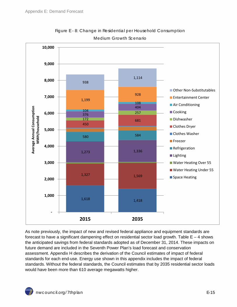
Appendix E: Demand Forecast
nwcouncil.org/7thplan E-15
Figure E - 8: Change in Residential per Household Consumption
Medium Growth Scenario
As note previously, the impact of new and revised federal appliance and equipment standards are forecast to have a significant dampening effect on residential sector load growth. Table E – 4 shows the anticipated savings from federal standards adopted as of December 31, 2014. These impacts on future demand are included in the Seventh Power Plan’s load forecast and conservation assessment. Appendix H describes the derivation of the Council estimates of impact of federal standards for each end-use. Energy use shown in this appendix includes the impact of federal standards. Without the federal standards, the Council estimates that by 2035 residential sector loads would have been more than 610 average megawatts higher.
1,618 1,418
1,327 1,569
1,273 1,336
580 584
450 681 172
257 376
404 104
108 1,199
928
938 1,114
-
1,000
2,000
3,000
4,000
5,000
6,000
7,000
8,000
9,000
10,000
2015 2035
Aver
age
Annu
al C
onsu
mpt
ion
MW
H/ho
useh
old
Other Non-Substitutables
Entertainment Center
Air Conditioning
Cooking
Dishwasher
Clothes Dryer
Clothes Washer
Freezer
Refrigeration
Lighting
Water Heating Over 55
Water Heating Under 55
Space Heating

Appendix E: Demand Forecast
nwcouncil.org/7thplan E-16
Table E - 4: Estimated Impact of federal standards by sector (aMW)-Medium Scenario 2015 2035
Residential 41 614 Commercial 25 467
Industrial 17 163 Transportation 0 11 Street lighting 1 8
Total Direct Impact 83 1,264
Residential Load Forecast
Range of residential load forecast is presented in Figure E – 9. Under the Seventh Power Plan’s medium forecast, residential sector electricity consumption is forecast to be flat. In the high forecast this sector is forecast to grow at an average annual growth rate of 0.5 percent per year between 2015 and 2035. In the low case scenario, residential sector load is projected to decline from roughly 8,300 average megawatts to about 8,100 average megawatts, largely due to the impact of federal standards, but also due to changing trends in ICE end uses. In the high growth scenario residential load is projected to grow by about 1,000 average megawatts by 2035, growing from about 8,300 to about 9,300 average megawatts.
Figure E - 9: Historic and Range of Forecast for Residential Load (aMW)*
• Note that loads shown for 1986-2012 are based on actual weather conditions while the load forecast for 2013-2035 assume normal weather.
0
1,000
2,000
3,000
4,000
5,000
6,000
7,000
8,000
9,000
10,000
1986
19
88
1990
19
92
1994
19
96
1998
20
00
2002
20
04
2006
20
08
2010
20
12
2014
20
16
2018
20
20
2022
20
24
2026
20
28
2030
20
32
2034
Regi
onal
Res
iden
tial L
oad
(aM
W)
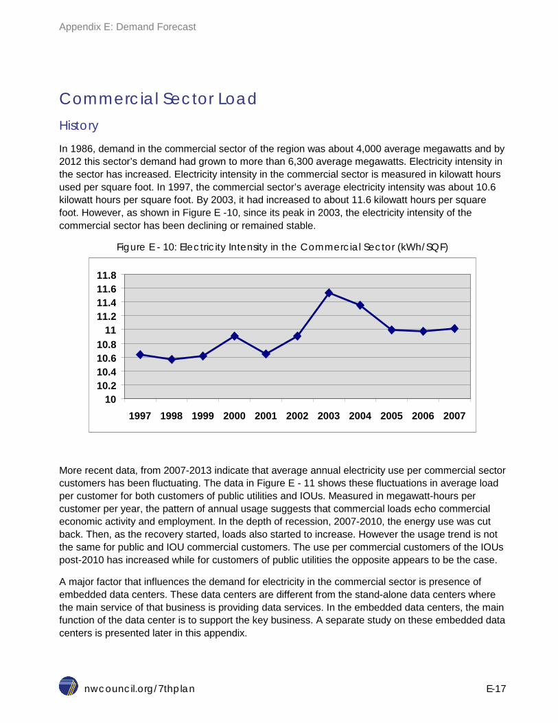
Appendix E: Demand Forecast
nwcouncil.org/7thplan E-17
Commercial Sector Load History
In 1986, demand in the commercial sector of the region was about 4,000 average megawatts and by 2012 this sector’s demand had grown to more than 6,300 average megawatts. Electricity intensity in the sector has increased. Electricity intensity in the commercial sector is measured in kilowatt hours used per square foot. In 1997, the commercial sector’s average electricity intensity was about 10.6 kilowatt hours per square foot. By 2003, it had increased to about 11.6 kilowatt hours per square foot. However, as shown in Figure E -10, since its peak in 2003, the electricity intensity of the commercial sector has been declining or remained stable.
Figure E - 10: Electricity Intensity in the Commercial Sector (kWh/SQF)
More recent data, from 2007-2013 indicate that average annual electricity use per commercial sector customers has been fluctuating. The data in Figure E - 11 shows these fluctuations in average load per customer for both customers of public utilities and IOUs. Measured in megawatt-hours per customer per year, the pattern of annual usage suggests that commercial loads echo commercial economic activity and employment. In the depth of recession, 2007-2010, the energy use was cut back. Then, as the recovery started, loads also started to increase. However the usage trend is not the same for public and IOU commercial customers. The use per commercial customers of the IOUs post-2010 has increased while for customers of public utilities the opposite appears to be the case.
A major factor that influences the demand for electricity in the commercial sector is presence of embedded data centers. These data centers are different from the stand-alone data centers where the main service of that business is providing data services. In the embedded data centers, the main function of the data center is to support the key business. A separate study on these embedded data centers is presented later in this appendix.
10 10.2 10.4 10.6 10.8
11 11.2 11.4 11.6 11.8
1997 1998 1999 2000 2001 2002 2003 2004 2005 2006 2007

Appendix E: Demand Forecast
nwcouncil.org/7thplan E-18
Figure E - 11: Electricity Intensity in the Commercial Sector (MWh/customer)
Commercial Load Forecast
Depending on the load growth scenario, commercial sector loads are forecast to grow by 0.9 to 1.1 percent per year between 2015 and 2035. As shown in Table E – 5, during this period, demand is expected to grow from about 6,300 average megawatts in 2012 to between about 8,000 and 8,500 average megawatts in 2035. The forecast growth rate for commercial sector for the Seventh Power Plan is lower than the Sixth Power Plan. Three major factors contribute to this slower growth forecast. First, there was a significant slowdown in commercial construction activities during the recession. Second, as in the residential sector, load growth in this sector will be dampened by new federal standards. Third, the increased availability and cost reductions of more efficient LED lighting will slow load growth. As was shown in Table E - 4, the estimated impact of federal standards lowers the commercial load by about 500 average megawatts by 2035. In addition, availability of LED lighting is expected to lower the demand for lighting significantly. This is evidenced by the fact that the growth rate in the lighting end-use in commercial sector is 0.4 percent below the overall growth rate for commercial sector.
Table E - 5: Enduse Level Forecast of Loads in Commercial Sector (aMW)
2012 2015 Low
2020 Low
2035 Low
2015 High
2020 High
2035 High
Commercial Total 6,377 6,731 6,897 7,996 6,905 7,215 8,596 Space Heating 464 491 499 540 504 520 556 Water Heating 143 155 159 175 159 167 192 Substitutables* 109 115 110 107 118 115 117 Refrigeration 918 889 751 587 907 781 645 Lighting 1,483 1,607 1,680 1,858 1,655 1,769 2,055 Air Conditioning 1,711 1,797 1,917 2,640 1,833 1,981 2,708 Non-Substitutables** 1,549 1,678 1,781 2,089 1,730 1,882 2,323
64 66 68 70 72 74 76 78 80
2007 2008 2009 2010 2011 2012 2013 2014
Annu
al A
vera
ge U
se (M
Wh/
yr)
Publics IOUs

Appendix E: Demand Forecast
nwcouncil.org/7thplan E-19
* Substitutable end uses include misc. appliances that can use multiple fuels, such as cooking, drying. **Non-substitutable end uses include, electronic equipments, misc. electric appliances that can only use electricity such as embedded data centers in commercial buildings. Embedded data centers, use a significant amount of electricity. For a discussion on Council’s estimate of load in embedded data centers, please see the section on this topic later in this appendix. The impact of new federal standards, fast moving trends toward more efficient lighting and improvements in embedded data centers all contribute to keep the forecast range of future load growth for the commercial sector rather narrow. Figure E – 12 shows the historical regional commercial sector loads and the Seventh Power Plan’s forecast range of future loads for this sector through 2035. As shown earlier, by 2035, as a result of federal standards commercial sector loads are lower by about 500 average megawatts. These improvements not only impact forecast of loads, but they also impact the conservation potential and conservation targets.
Figure E - 12: Forecast Commercial Electricity Loads (aMW)
Embedded Data Center Loads As mentioned above, embedded data centers are one of the end-uses covered under the non-substitutable loads category in the commercial sector. There are a wide variety of data centers in this category. From small closet-size data centers housing servers, storage devices, communication, and back up devices serving a small restaurant to large room size-data centers serving large retail chains. There is very limited information about the baseline operating characteristics and load in these data centers. They are typically not separately metered and their energy usage is typically blended with the usage by other end uses, such as lighting in the business.
0
1,000
2,000
3,000
4,000
5,000
6,000
7,000
8,000
9,000
10,000
Aver
age
Meg
awat
ts

Appendix E: Demand Forecast
nwcouncil.org/7thplan E-20
To shed some light on demand from these data centers, Council commissioned a study to use the available Data Center survey results from NEEA’s 2014 commercial building stock assessment3 along with other industry data and develop an estimate of current consumption for embedded data centers as well as a projection of the consumption under various technology trajectories. The results of this analysis are reported in Table E – 6.
Table E - 6: 2013 Estimated Use by Application and Data Center Types (aMW)
Server closet Server room Localized Mid-tier Total
Servers 20.4 85.0 8.3 45.7 159.5 Storage - - 1.7 9.1 10.8 Network 1.1 9.4 1.1 6.1 17.7 Transformers - 4.7 0.6 3.0 8.3 UPS 4.3 18.9 2.2 12.2 37.6 Lighting 1.1 1.9 0.2 1.2 4.4 Cooling 9.3 33.7 4.3 24.8 72.1 Total 36.1 153.7 18.4 102.3 310.4
For most mature industries and end-uses it is easier to forecast the future growth in loads. In the case of data centers, given the speed of change in the technology, be it servers, or storage or network devices, it is more difficult to forecast future load growth. Making a long-term forecast for such fast changing sector would be more subject to significant uncertainty. Figure E – 13 presents a possible range for the trajectory of electricity demand for embedded data centers. For example, if all the current embedded data centers move their services to “the cloud,” the Council estimates there will be about 200 average megawatt reductions in load region wide. By 2035, projected Business as Usual loads from embedded data centers are forecast to be about 650 average megawatts. If the services now performed by embedded data centers are transferred to “the cloud,” future loads could be as low as 100 average megawatts. A more detailed look at the embedded data centers is presented later in this appendix.
3 http://neea.org/resource-center/regional-data-resources/commercial-building-stock-assessment

Appendix E: Demand Forecast
nwcouncil.org/7thplan E-21
Figure E - 13: Possible range of Embedded Data Center Loads with different technology paths (aMW)
To forecast embedded data center load, the Council used Business as Usual trajectory subject to different commercial sector growth rates. As shown in Figure E – 14, data center loads are projected to grow from current estimate of about 350 average megawatts to between 600 and 670 average megawatts by 2035.
Figure E - 14: Forecast Embedded Data Center Loads (aMW)
0 100 200 300 400 500 600 700
2014
20
15
2016
20
17
2018
20
19
2020
20
21
2022
20
23
2024
20
25
2026
20
27
2028
20
29
2030
20
31
2032
20
33
2034
20
35
Aver
age
Meg
awat
ts
BAU Best practice adoption
Commercial technology adoption Cutting edge technology adoption
Shift closets, rooms to cloud
0
100
200
300
400
500
600
700
800
2015
20
16
2017
20
18
2019
20
20
2021
20
22
2023
20
24
2025
20
26
2027
20
28
2029
20
30
2031
20
32
2033
20
34
2035
Aver
age
Meg
awat
ts
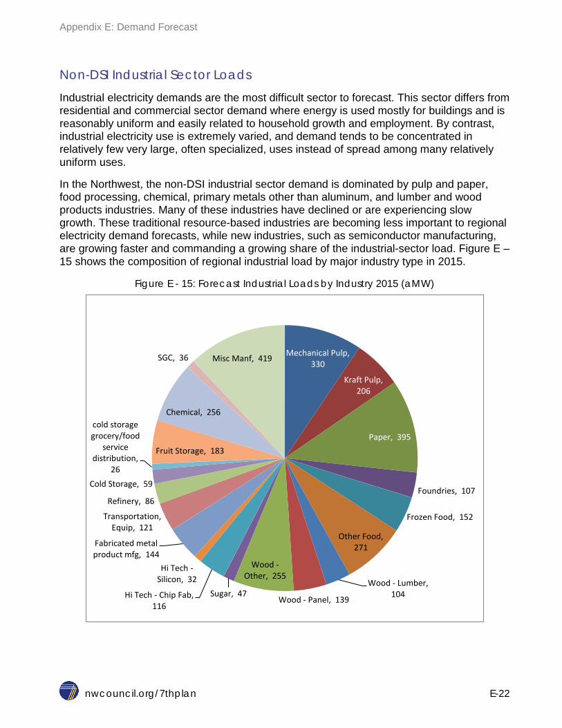
Appendix E: Demand Forecast
nwcouncil.org/7thplan E-22
Non-DSI Industrial Sector Loads
Industrial electricity demands are the most difficult sector to forecast. This sector differs from residential and commercial sector demand where energy is used mostly for buildings and is reasonably uniform and easily related to household growth and employment. By contrast, industrial electricity use is extremely varied, and demand tends to be concentrated in relatively few very large, often specialized, uses instead of spread among many relatively uniform uses.
In the Northwest, the non-DSI industrial sector demand is dominated by pulp and paper, food processing, chemical, primary metals other than aluminum, and lumber and wood products industries. Many of these industries have declined or are experiencing slow growth. These traditional resource-based industries are becoming less important to regional electricity demand forecasts, while new industries, such as semiconductor manufacturing, are growing faster and commanding a growing share of the industrial-sector load. Figure E – 15 shows the composition of regional industrial load by major industry type in 2015.
Figure E - 15: Forecast Industrial Loads by Industry 2015 (aMW)
Mechanical Pulp, 330
Kraft Pulp, 206
Paper, 395
Foundries, 107
Frozen Food, 152
Other Food, 271
Wood - Lumber, 104 Wood - Panel, 139
Wood - Other, 255
Sugar, 47 Hi Tech - Chip Fab, 116
Hi Tech - Silicon, 32
Fabricated metal product mfg, 144
Transportation, Equip, 121
Refinery, 86
Cold Storage, 59
cold storage grocery/food
service distribution,
26
Fruit Storage, 183
Chemical, 256
SGC, 36 Misc Manf, 419

Appendix E: Demand Forecast
nwcouncil.org/7thplan E-23
The electricity intensity of Northwest industries has decreased substantially as a result of structural changes. Table E – 7 shows the trend in electricity use per employee in the non-DSI industries for selected years since 1985.
Table E - 7: Changing Electric Intensity of Industries in the Northwest
Year Non-DSI Electricity Intensity (MWh/Industrial employees)
1985 59.2 1990 58.3 2000 56.4 2002 48.7 2007 46.8
Since the recession of 2007, the decline is usage has continued. Additional data, shown in Figure E – 16, covering the period from the 2007 to 2014 reveals that consumption per industrial customer account continues to decline. However, while use per industrial customer has been declining, total regional industrial output has been on the rise.
Figure E - 16: Electricity Intensity in the Industrial Sector
*Customers count used here is based on utility-reported industrial counts which includes small, large, and very large industrial account customers.
Non-DSI Industrial Load Forecast
In the Seventh Power Plan, non-DSI industrial consumption is forecast to grow at average annual growth rate of between 1 and 1.4 percent. As shown in Figure E – 17, electricity consumption in this sector is forecast to grow from about 3,500 in 2015 to between 4,200 and 4,600 by 2035.
-
200
400
600
800
1,000
1,200
2007 2008 2009 2010 2011 2012 2013 2014 Aver
age
Annu
al U
se p
er C
usto
mer
(M
WH/
yr)*
Publics IOUs
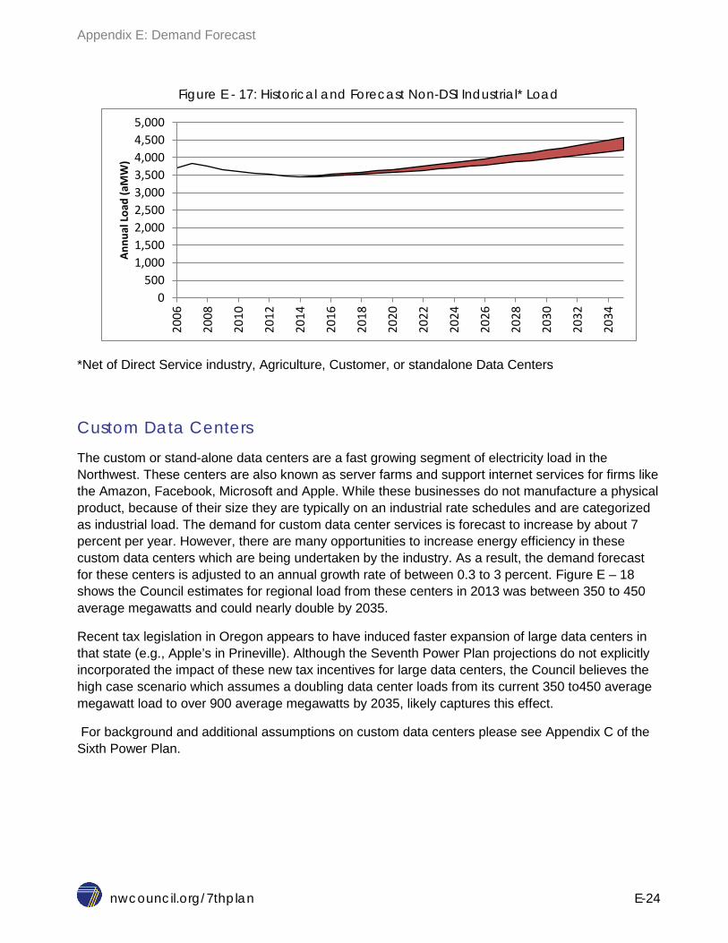
Appendix E: Demand Forecast
nwcouncil.org/7thplan E-24
Figure E - 17: Historical and Forecast Non-DSI Industrial* Load
*Net of Direct Service industry, Agriculture, Customer, or standalone Data Centers
Custom Data Centers
The custom or stand-alone data centers are a fast growing segment of electricity load in the Northwest. These centers are also known as server farms and support internet services for firms like the Amazon, Facebook, Microsoft and Apple. While these businesses do not manufacture a physical product, because of their size they are typically on an industrial rate schedules and are categorized as industrial load. The demand for custom data center services is forecast to increase by about 7 percent per year. However, there are many opportunities to increase energy efficiency in these custom data centers which are being undertaken by the industry. As a result, the demand forecast for these centers is adjusted to an annual growth rate of between 0.3 to 3 percent. Figure E – 18 shows the Council estimates for regional load from these centers in 2013 was between 350 to 450 average megawatts and could nearly double by 2035.
Recent tax legislation in Oregon appears to have induced faster expansion of large data centers in that state (e.g., Apple’s in Prineville). Although the Seventh Power Plan projections do not explicitly incorporated the impact of these new tax incentives for large data centers, the Council believes the high case scenario which assumes a doubling data center loads from its current 350 to450 average megawatt load to over 900 average megawatts by 2035, likely captures this effect.
For background and additional assumptions on custom data centers please see Appendix C of the Sixth Power Plan.
0 500
1,000 1,500 2,000 2,500 3,000 3,500 4,000 4,500 5,000
2006
2008
2010
2012
2014
2016
2018
2020
2022
2024
2026
2028
2030
2032
2034
Annu
al L
oad
(aM
W)

Appendix E: Demand Forecast
nwcouncil.org/7thplan E-25
Figure E - 18: Projected Load from Custom Data Centers
Direct Service Industries
Historically, direct service industries (DSIs) were industrial plants that purchased their electricity directly from the Bonneville Power Administration. These industries played an integral role in the development of the region’s hydroelectric system, for this industrial sector grew as the region’s hydroelectric system grew. The vast majority of companies in this category are aluminum smelters. When all of the region’s 10 aluminum smelters were operating at capacity, they could consume about 3,150 average megawatts of electricity. However, after Bonneville’s electricity prices increased following the power crisis of 2000-2001, many smelters shut down permanently. Currently, only a few aluminum smelting pot lines operate in the region, consuming about 750 average megawatts of energy. The Seventh Power Plan assumes that DSI electricity load will be around 600 to 700 average megawatts for the forecast period. Although the portion of Alcoa's Wenatchee aluminum smelter that is served from non-Bonneville sources is not technically a DSI (i.e., it is not served by Bonneville), that load is included in the DSI category in the Seventh Power Plan so it can be compared to prior Power Plans.
The Council used Bonneville’s forecast of future DSI loads from the agency’s 2014 White Book for the draft Seventh Power Plan. In November 2015 Alcoa Inc. announced that it is idling its two smelting operations in state of Washington. For the final Seventh Power Plan aluminum smelter DSI loads in 2016-2017 were lowered to reflect the Alcoa’s plans. For the long-term medium forecast, aluminum smelter loads were lowered from about 770 to about 338 average megawatts, reflecting the possibility that only one of the two smelting operations will return. The Seventh Power Plan’s high range of load uncertainty in RPM was increased to reflect possibility of return for both the second aluminum smelter and possibility of additional industrial load from a number of planned
-
100
200
300
400
500
600
700
800
900
1,000
2013
2014
2015
2016
2017
2018
2019
2020
2021
2022
2023
2024
2025
2026
2027
2028
2029
2030
2031
2032
2033
2034
2035
Annu
al L
oad
(aM
W)
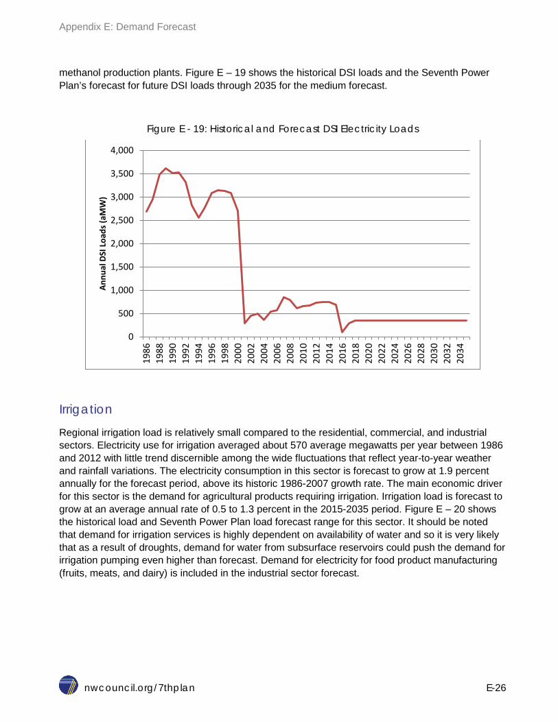
Appendix E: Demand Forecast
nwcouncil.org/7thplan E-26
methanol production plants. Figure E – 19 shows the historical DSI loads and the Seventh Power Plan’s forecast for future DSI loads through 2035 for the medium forecast.
Figure E - 19: Historical and Forecast DSI Electricity Loads
Irrigation
Regional irrigation load is relatively small compared to the residential, commercial, and industrial sectors. Electricity use for irrigation averaged about 570 average megawatts per year between 1986 and 2012 with little trend discernible among the wide fluctuations that reflect year-to-year weather and rainfall variations. The electricity consumption in this sector is forecast to grow at 1.9 percent annually for the forecast period, above its historic 1986-2007 growth rate. The main economic driver for this sector is the demand for agricultural products requiring irrigation. Irrigation load is forecast to grow at an average annual rate of 0.5 to 1.3 percent in the 2015-2035 period. Figure E – 20 shows the historical load and Seventh Power Plan load forecast range for this sector. It should be noted that demand for irrigation services is highly dependent on availability of water and so it is very likely that as a result of droughts, demand for water from subsurface reservoirs could push the demand for irrigation pumping even higher than forecast. Demand for electricity for food product manufacturing (fruits, meats, and dairy) is included in the industrial sector forecast.
0
500
1,000
1,500
2,000
2,500
3,000
3,500
4,000 19
86
1988
19
90
1992
19
94
1996
19
98
2000
20
02
2004
20
06
2008
20
10
2012
20
14
2016
20
18
2020
20
22
2024
20
26
2028
20
30
2032
20
34
Annu
al D
SI L
oads
(aM
W)
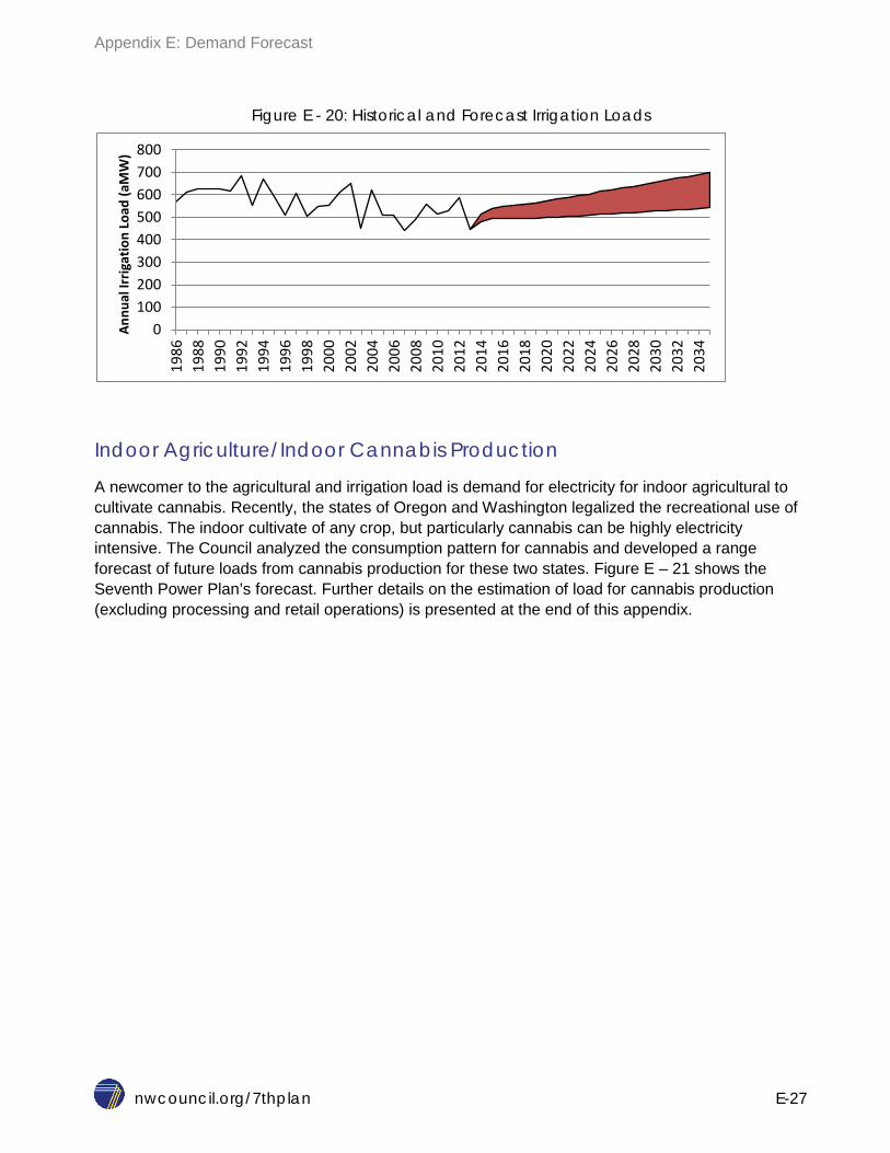
Appendix E: Demand Forecast
nwcouncil.org/7thplan E-27
Figure E - 20: Historical and Forecast Irrigation Loads
Indoor Agriculture/Indoor Cannabis Production
A newcomer to the agricultural and irrigation load is demand for electricity for indoor agricultural to cultivate cannabis. Recently, the states of Oregon and Washington legalized the recreational use of cannabis. The indoor cultivate of any crop, but particularly cannabis can be highly electricity intensive. The Council analyzed the consumption pattern for cannabis and developed a range forecast of future loads from cannabis production for these two states. Figure E – 21 shows the Seventh Power Plan’s forecast. Further details on the estimation of load for cannabis production (excluding processing and retail operations) is presented at the end of this appendix.
0 100 200 300 400 500 600 700 800
1986
19
88
1990
19
92
1994
19
96
1998
20
00
2002
20
04
2006
20
08
2010
20
12
2014
20
16
2018
20
20
2022
20
24
2026
20
28
2030
20
32
2034
Annu
al Ir
rigat
ion
Load
(aM
W)

Appendix E: Demand Forecast
nwcouncil.org/7thplan E-28
Figure E - 21: Indoor Agriculture/Cannabis Load Forecast
Transportation
The use of electricity in the transportation sector, consisting mainly of mass transit systems in major metropolitan cities in the region, has been about 2 to 3 average megawatts. However, in the past few years there has been a new entry into this market, the plug-in electric and all electric vehicles. This has caused a significant increase in the use of electricity for transportation. The Council has tracked the growing number of plug-in electric (PHEVs) in the region. Preliminary analysis, reflected in the Seventh Power Plan’s forecast shown in Figure E- 22, indicates that demand from plug-in electric vehicles could add 160 to 625 average megawatts to regional electricity use by 2035.
0
50
100
150
200
250
300
350
2014 2015 2020 2025 2030 2035
Annu
al L
oad
(aM
W)
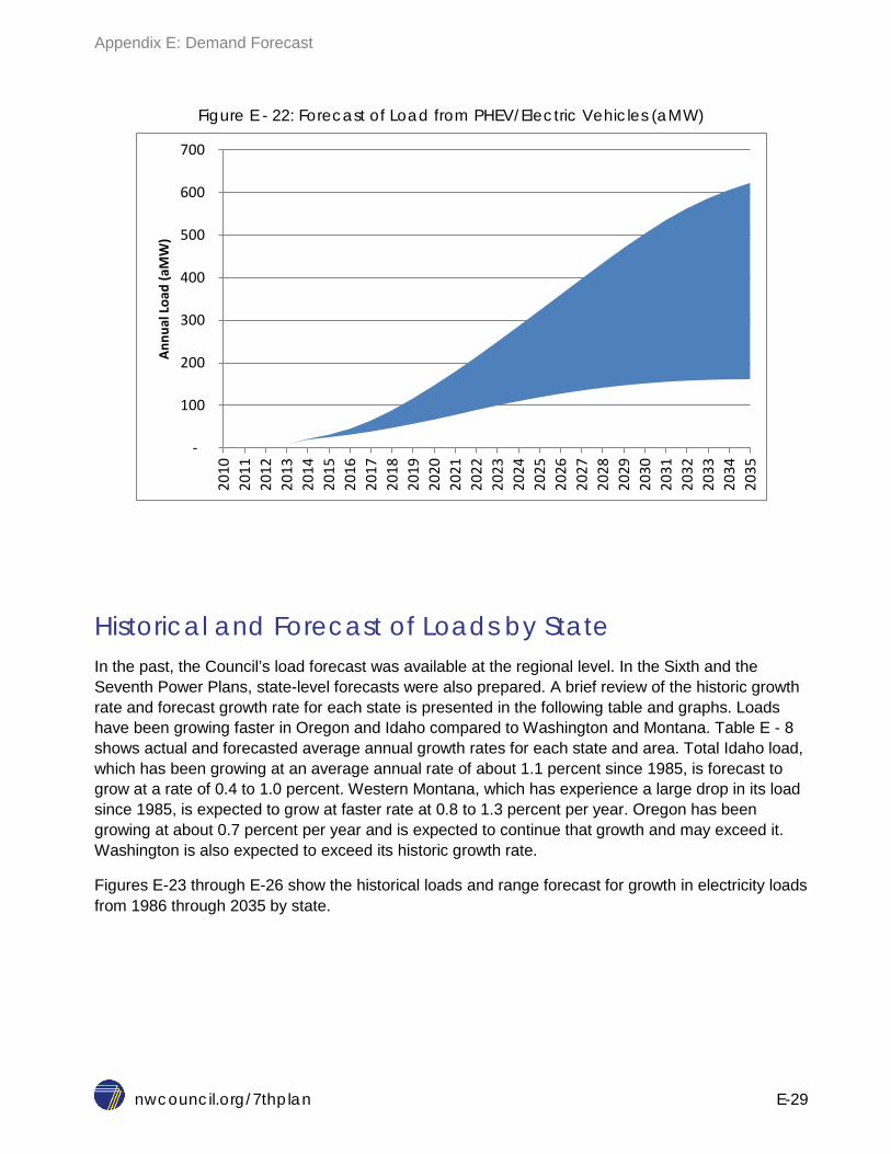
Appendix E: Demand Forecast
nwcouncil.org/7thplan E-29
Figure E - 22: Forecast of Load from PHEV/Electric Vehicles (aMW)
Historical and Forecast of Loads by State In the past, the Council’s load forecast was available at the regional level. In the Sixth and the Seventh Power Plans, state-level forecasts were also prepared. A brief review of the historic growth rate and forecast growth rate for each state is presented in the following table and graphs. Loads have been growing faster in Oregon and Idaho compared to Washington and Montana. Table E - 8 shows actual and forecasted average annual growth rates for each state and area. Total Idaho load, which has been growing at an average annual rate of about 1.1 percent since 1985, is forecast to grow at a rate of 0.4 to 1.0 percent. Western Montana, which has experience a large drop in its load since 1985, is expected to grow at faster rate at 0.8 to 1.3 percent per year. Oregon has been growing at about 0.7 percent per year and is expected to continue that growth and may exceed it. Washington is also expected to exceed its historic growth rate.
Figures E-23 through E-26 show the historical loads and range forecast for growth in electricity loads from 1986 through 2035 by state.
-
100
200
300
400
500
600
700
2010
20
11
2012
20
13
2014
20
15
2016
20
17
2018
20
19
2020
20
21
2022
20
23
2024
20
25
2026
20
27
2028
20
29
2030
20
31
2032
20
33
2034
20
35
Annu
al L
oad
(aM
W)

Appendix E: Demand Forecast
nwcouncil.org/7thplan E-30
Table E - 8: Historic and forecasted range of growth in state loads
(Average annual growth rate in percent)
Idaho Western Montana Oregon Washington
1986-2012 actual 1.1 - 0.5 0.7 0.3
2015-2035 range 0.4 -1.0 0.8 -1.3 0.7 -1.2 0.4 - 0.9
Additional details on the state and sector level loads are available in the companion workbook available from Council’s website. http://www.nwcouncil.org/energy/powerplan/7/technical
Figure E - 23: Historic and Forecast Electric Load for State of Idaho
0
500
1000
1500
2000
2500
3000
3500
1986
19
88
1990
19
92
1994
19
96
1998
20
00
2002
20
04
2006
20
08
2010
20
12
2014
20
16
2018
20
20
2022
20
24
2026
20
28
2030
20
32
2034
Annu
al L
oad
(aM
W)

Appendix E: Demand Forecast
nwcouncil.org/7thplan E-31
Figure E - 24: Historic and Forecast Electric Load for Western Montana
Figure E - 25: Historic and Forecast Electric load for State of Oregon
0
200
400
600
800
1000
1200
1400
1600
1986
19
88
1990
19
92
1994
19
96
1998
20
00
2002
20
04
2006
20
08
2010
20
12
2014
20
16
2018
20
20
2022
20
24
2026
20
28
2030
20
32
2034
Annu
al L
oad
(aM
w)
0
1,000
2,000
3,000
4,000
5,000
6,000
7,000
8,000
9,000
1986
19
88
1990
19
92
1994
19
96
1998
20
00
2002
20
04
2006
20
08
2010
20
12
2014
20
16
2018
20
20
2022
20
24
2026
20
28
2030
20
32
2034
Annu
al L
oad
(aM
W)

Appendix E: Demand Forecast
nwcouncil.org/7thplan E-32
Figure E - 26: Historic and Forecast Electric Load for State of Washington
Monthly Pattern of Load In order to make sure that sufficient resources are available to meet demand, it is necessary to forecast the timing of peak load. Figure E – 27 shows that electricity use is not evenly distributed throughout the year. The electric system in the Northwest is a winter peaking system, which means that the maximum use of electricity occurs during the winter months. The historic demand for electricity for the region shows a “W”-shaped profile. Table E – 9 shows that approximately 9-10 percent of annual electricity in the region is consumed each month in the winter months of January and December. This table also shows that in the shoulder months (March through June, and September through November) monthly energy consumption is about 8 percent of the annual total. In summer months, slightly above 8 percent of the annual total is consumed each month. Similar patterns can be observed in each one of the four states, with electricity demand in Idaho slightly higher in summer and slightly lower than the regional average in winter months.
0
2000
4000
6000
8000
10000
12000
14000
1986
19
88
1990
19
92
1994
19
96
1998
20
00
2002
20
04
2006
20
08
2010
20
12
2014
20
16
2018
20
20
2022
20
24
2026
20
28
2030
20
32
2034
Annu
al L
oad
(aM
W)

Appendix E: Demand Forecast
nwcouncil.org/7thplan E-33
Figure E - 27: Monthly Pattern of Demand for Electricity
Table E - 9: Monthly Pattern of Demand for Electricity
ID MT OR WA Region
Dec 9% 9% 9% 9% 9%
January 9% 10% 10% 10% 10%
July 10% 8% 8% 8% 8%
Aug 9% 8% 8% 8% 8%
REGIONAL PEAK LOAD The temporal pattern of load and peaks are becoming more important. The region has historically been constrained by average annual energy supplies. However, in the future the Council forecast that it is more likely to be constrained by limits to its peaking capability.
To better forecast the temporal pattern of demand and hourly load, the Council has developed two models:
A short-term load forecasting model that projects 3-5 years into the future on an hourly basis. The short-term model is used for the resource adequacy analysis.
A long-term load forecasting model that projects 20 years into the future on a monthly basis.
This appendix discusses the long-term forecasting model.

Appendix E: Demand Forecast
nwcouncil.org/7thplan E-34
Seasonal Variation in Load Regional load has seasonal variability driven by temperature changes. Although the Northwest is a winter-peaking region, there can be a significant range in winter load. To illustrate this, Figure E -28 shows three load levels based on differing weather conditions. The dashed line shows the daily average megawatts of energy under normal weather conditions. Winter daily energy demand is about 28,000 average megawatts and summer average demand is about 24,000 average megawatts under these conditions. Also under normal weather, the peak-hour load in winter reaches over 33,000 megawatts, and the summer peak increases to about 28,000 megawatts. If weather conditions are extreme, then the hourly load can increase substantially and has reached more than 41,000 megawatts in winter and more than 30,000 megawatts in the summer.
Figure E - 28: Range of Variation in Load
Average, Peak, and Off-peak Loads
The electrical system in the Northwest must meet loads every hour throughout the year. Not only average load but also peak and off-peak loads must be met. This section present the range of forecast for peak and off-peak loads developed for the Seventh Power Plan. Figure E – 29 shows the historical peak loads from 1995 to 2012. These peak loads reflect actual weather conditions in each of those years. Figure E – 29 also shows the Seventh Power Plan’s peak load projections for the forecast period, but under normal weather conditions. A review of Figure E-29 shows that winter peak loads between 1995 and 2012 did not change. In fact, and due to impact of loss of DSI, winter peak loads have actually decreased by about 0.4 percent per year over this time period. However, since the loss of the DSI loads has already occurred, the Seventh Power Plan forecast annual winter peak loads to grow by 0.4 to 0.8 percent annually.
17,000
22,000
27,000
32,000
37,000
42,000
47,000
January
February
March
April
May
June
July
August
September
October
November
December
Hourly Peak MW with extreme Temperature Condition
Daily Average MW with Normal Weather
Hourly Peak MW with Normal Weather
Illustrative Example

Appendix E: Demand Forecast
nwcouncil.org/7thplan E-35
Figure E - 29: Historical and Forecast Range of Winter Peak Loads
The Seventh Power Plan forecast that seasonal peak loads will grow at different rates. Figure E – 30 shows historical summer peak loads and the Seventh Power Plan’s forecast for summer peaks through 2035. A comparison of Figure E - 29 and E – 30 shows that by 2035, expected summer peaks are within 95 percent of the winter peak loads.
Figure E - 30: Historical and Forecast Range of Summer Peak Loads
Loads versus Demand/Sales
The load forecast data presented earlier were measured at the generator busbar; in other words, they include transmission and distribution losses. This energy loss from transmission and distribution varies depending on temperature conditions and the mix of sectors. Higher temperatures coincident with higher loads mean a greater loss of energy. Transmission and distribution losses also increase as the regional load shifts to the residential or commercial sector. Large industrial customers, like
0 5,000
10,000 15,000 20,000 25,000 30,000 35,000 40,000
1995
19
97
1999
20
01
2003
20
05
2007
20
09
2011
20
13
2015
20
17
2019
20
21
2023
20
25
2027
20
29
2031
20
33
2035
Win
ter P
eak
Load
(MW
)
0
5,000
10,000
15,000
20,000
25,000
30,000
35,000
40,000
1995
19
97
1999
20
01
2003
20
05
2007
20
09
2011
20
13
2015
20
17
2019
20
21
2023
20
25
2027
20
29
2031
20
33
2035
Sum
mer
Pea
k Lo
ad (M
W)
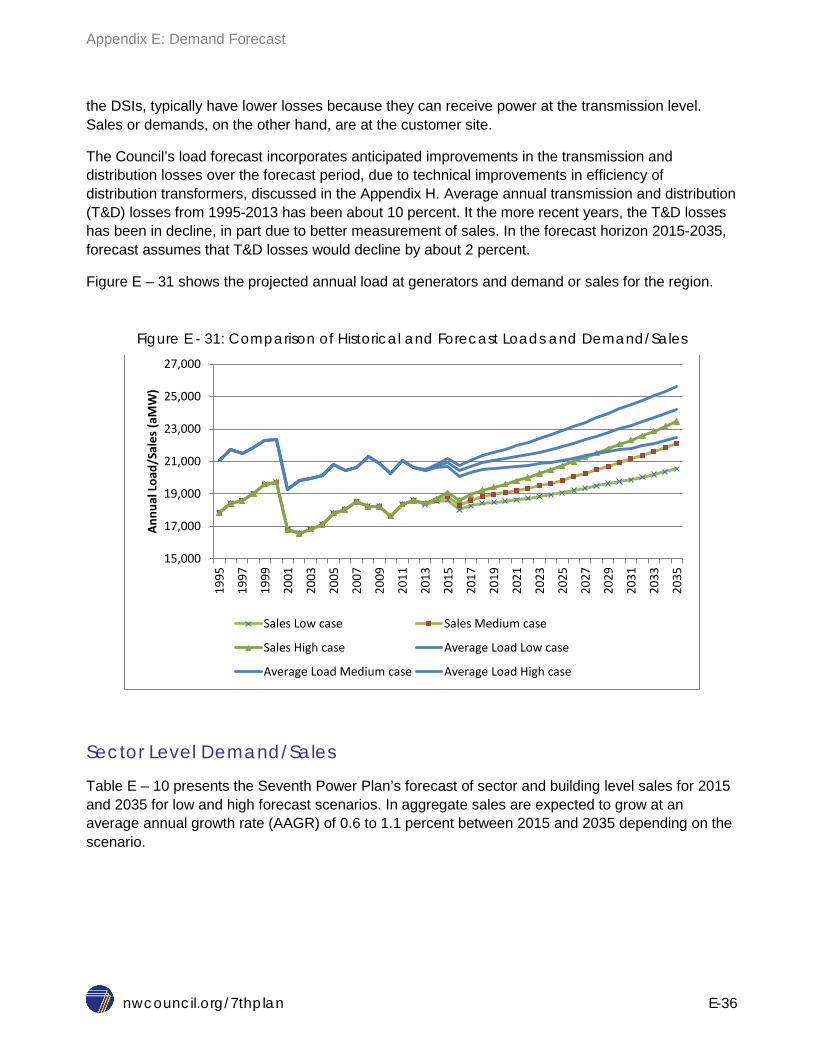
Appendix E: Demand Forecast
nwcouncil.org/7thplan E-36
the DSIs, typically have lower losses because they can receive power at the transmission level. Sales or demands, on the other hand, are at the customer site.
The Council’s load forecast incorporates anticipated improvements in the transmission and distribution losses over the forecast period, due to technical improvements in efficiency of distribution transformers, discussed in the Appendix H. Average annual transmission and distribution (T&D) losses from 1995-2013 has been about 10 percent. It the more recent years, the T&D losses has been in decline, in part due to better measurement of sales. In the forecast horizon 2015-2035, forecast assumes that T&D losses would decline by about 2 percent.
Figure E – 31 shows the projected annual load at generators and demand or sales for the region.
Figure E - 31: Comparison of Historical and Forecast Loads and Demand/Sales
Sector Level Demand/Sales
Table E – 10 presents the Seventh Power Plan’s forecast of sector and building level sales for 2015 and 2035 for low and high forecast scenarios. In aggregate sales are expected to grow at an average annual growth rate (AAGR) of 0.6 to 1.1 percent between 2015 and 2035 depending on the scenario.
15,000
17,000
19,000
21,000
23,000
25,000
27,000
1995
1997
1999
2001
2003
2005
2007
2009
2011
2013
2015
2017
2019
2021
2023
2025
2027
2029
2031
2033
2035
Annu
al L
oad/
Sale
s (a
MW
)
Sales Low case Sales Medium case
Sales High case Average Load Low case
Average Load Medium case Average Load High case
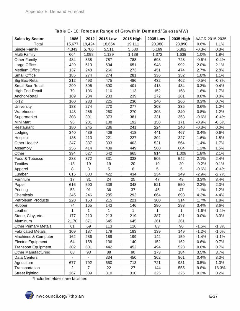
Appendix E: Demand Forecast
nwcouncil.org/7thplan E-37
Table E - 10: Forecast Range of Growth in Demand/Sales (aMW)
Sales by Sector 1986 2012 2015 Low 2015 High 2035 Low 2035 High AAGR 2015-2035 Total 15,677 19,424 18,654 19,111 20,988 23,890 0.6% 1.1%
Single Family 4,343 5,786 5,511 5,530 5,169 5,862 -0.3% 0.3% Multi Family 664 1,098 1,129 1,138 1,372 1,639 1.0% 1.8% Other Family 484 838 787 788 698 728 -0.6% -0.4% Large Office 429 613 634 651 948 992 2.0% 2.1% Medium Office 137 248 266 273 451 474 2.7% 2.8% Small Office 185 274 274 281 336 352 1.0% 1.1% Big Box-Retail 212 493 475 486 432 462 -0.5% -0.3% Small Box-Retail 299 396 390 401 413 434 0.3% 0.4% High End-Retail 79 106 110 113 152 158 1.6% 1.7% Anchor-Retail 189 234 233 239 272 281 0.8% 0.8% K-12 160 233 225 230 240 266 0.3% 0.7% University 183 274 270 277 303 335 0.6% 1.0% Warehouse 148 256 260 270 303 340 0.8% 1.2% Supermarket 308 391 373 381 331 353 -0.6% -0.4% Mini Mart 96 201 188 192 158 171 -0.9% -0.6% Restaurant 180 245 236 241 224 240 -0.3% 0.0% Lodging 340 439 409 418 441 467 0.4% 0.6% Hospital 135 213 221 227 302 327 1.6% 1.8% Other Health* 247 387 393 403 521 564 1.4% 1.7% Assembly 256 414 439 449 560 604 1.2% 1.5% Other 394 627 642 665 914 1,008 1.8% 2.1% Food & Tobacco 283 372 331 338 505 542 2.1% 2.4% Textiles 13 19 19 20 19 20 -0.2% 0.1% Apparel 8 8 5 6 5 5 -0.6% -0.4% Lumber 615 600 422 434 234 249 -2.9% -2.7% Furniture 17 31 24 25 47 49 3.3% 3.4% Paper 616 590 339 348 521 550 2.2% 2.3% Printing 53 91 36 37 45 47 1.1% 1.2% Chemicals 245 246 285 292 664 693 4.3% 4.4% Petroleum Products 220 153 215 221 300 314 1.7% 1.8% Rubber 74 165 143 146 280 293 3.4% 3.6% Leather 1 1 1 1 1 1 -1.6% -1.4% Stone, Clay, etc. 177 210 213 219 387 421 3.0% 3.3% Aluminum 2,170 671 645 645 261 261
Other Primary Metals 61 69 113 116 83 90 -1.5% -1.3% Fabricated Metals 109 187 179 183 139 149 -1.2% -1.0% Machines & Computer 162 286 189 199 142 159 -1.4% -1.1% Electric Equipment 64 158 136 140 152 162 0.6% 0.7% Transport Equipment 302 601 442 452 494 523 0.6% 0.7% Other Manufacturing 68 93 88 90 173 184 3.5% 3.7% Data Centers - - 334 450 362 861 0.4% 3.3% Agriculture 677 792 650 713 721 931 0.5% 1.3% Transportation 2 7 22 27 144 555 9.8% 16.3% Street lighting 267 309 310 310 325 325 0.2% 0.2%
*Includes elder care facilities
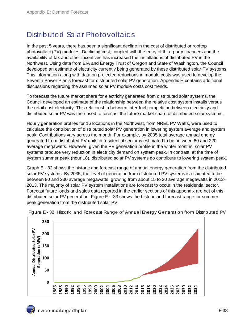
Appendix E: Demand Forecast
nwcouncil.org/7thplan E-38
Distributed Solar Photovoltaics In the past 5 years, there has been a significant decline in the cost of distributed or rooftop photovoltaic (PV) modules. Declining cost, coupled with the entry of third-party financers and the availability of tax and other incentives has increased the installations of distributed PV in the Northwest. Using data from EIA and Energy Trust of Oregon and State of Washington, the Council developed an estimate of electricity currently being generated by these distributed solar PV systems. This information along with data on projected reductions in module costs was used to develop the Seventh Power Plan’s forecast for distributed solar PV generation. Appendix H contains additional discussions regarding the assumed solar PV module costs cost trends.
To forecast the future market share for electricity generated from distributed solar systems, the Council developed an estimate of the relationship between the relative cost system installs versus the retail cost electricity. This relationship between inter-fuel competition between electricity and distributed solar PV was then used to forecast the future market share of distributed solar systems.
Hourly generation profiles for 16 locations in the Northwest, from NREL PV Watts, were used to calculate the contribution of distributed solar PV generation in lowering system average and system peak. Contributions vary across the month. For example, by 2035 total average annual energy generated from distributed PV units in residential sector is estimated to be between 80 and 220 average megawatts. However, given the PV generation profile in the winter months, solar PV systems produce very reduction in electricity demand on system peak. In contrast, at the time of system summer peak (hour 18), distributed solar PV systems do contribute to lowering system peak.
Graph E - 32 shows the historic and forecast range of annual energy generation from the distributed solar PV systems. By 2035, the level of generation from distributed PV systems is estimated to be between 80 and 230 average megawatts, growing from about 15 to 20 average megawatts in 2012-2013. The majority of solar PV system installations are forecast to occur in the residential sector. Forecast future loads and sales data reported in the earlier sections of this appendix are net of this distributed solar PV generation. Figure E – 33 shows the historic and forecast range for summer peak generation from the distributed solar PV.
Figure E - 32: Historic and Forecast Range of Annual Energy Generation from Distributed PV
0
50
100
150
200
250
1986
19
88
1990
19
92
1994
19
96
1998
20
00
2002
20
04
2006
20
08
2010
20
12
2014
20
16
2018
20
20
2022
20
24
2026
20
28
2030
20
32
2034
Annu
al D
istr
ibut
ed S
olar
PV
Gen
erat
ion
(aM
W)

Appendix E: Demand Forecast
nwcouncil.org/7thplan E-39
Figure E - 33: Historic and Forecast Range of Summer Peak Generation from Distributed PV
Calculations for Alternative Load Forecast Concepts Three different but related load forecasts are produced for use in the Council’s resource planning process. The first of these forecasts is called a “price-effect” forecast, which is the forecast presented to this point. The price-effect forecast is the official demand forecast required by the Northwest Power Act.
The price-effect forecast reflects customers’ choices in response to electricity and fuel prices and technology costs, without any new programmatic conservation initiatives. That is, this forecast does not include the potential impacts of future utility development of cost-effective conservation resources, nor changes in codes and standards beyond those already adopted as of December 2014. However, expected savings from existing and approved codes and standards (i.e., those known as of December 2014) are incorporated in the price-effect forecast, consequently reducing the forecast and removing that potential from Council’s estimate of remaining conservation opportunities.
To eliminate double-counting the conservation potential, the load-forecasting model produces two other long-term forecasts that are required for estimating conservation potential and running the resource portfolio model: the frozen efficiency forecast and the sales forecast.
1. Frozen-efficiency (FE) forecast, assumed that efficiency level is fixed or frozen at the base year of the plan (in the case of the Seventh Power Plan, base year is 2015). For example, if a new refrigerator in 2015 uses 300 kilowatt-hours of electricity per year, in the FE forecast this level of consumption is kept constant over the 20-year planning horizon. However, if there is a known federal standard that goes into effect at a future point in time, say 2022, which is expected to lower the electricity consumption of a new refrigerator to 250 kilowatt-hours per year, then post 2022 any new refrigerator added to stock is assumed to use 250 kilowatt-hours per year. In this way, the difference in consumption, 50 kilowatt-hours, is treated as a reduction in the load forecast rather than part of conservation target. This forecast attempts to eliminate the double-counting of conservation savings. The frozen technical-efficiency levels used in the FE load forecast also form basis for estimating the remaining conservation potential. The frozen-efficiency load forecast serves
0
100
200
300
400
500
600
700
1986
19
88
1990
19
92
1994
19
96
1998
20
00
2002
20
04
2006
20
08
2010
20
12
2014
20
16
2018
20
20
2022
20
24
2026
20
28
2030
20
32
2034
Sum
mer
Pea
k G
ener
atio
n fr
om
Dist
ribut
ed so
lar P
V (M
W)
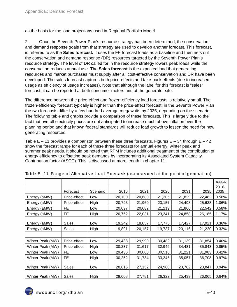
Appendix E: Demand Forecast
nwcouncil.org/7thplan E-40
as the basis for the load projections used in Regional Portfolio Model. 2. Once the Seventh Power Plan’s resource strategy has been determined, the conservation and demand response goals from that strategy are used to develop another forecast. This forecast, is referred to as the Sales forecast. It uses the FE forecast loads as a baseline and then nets out the conservation and demand response (DR) resources targeted by the Seventh Power Plan’s resource strategy. The level of DR called for in the resource strategy lowers peak loads while the conservation reduces annual use. The Sales forecast is the expected load that generating resources and market purchases must supply after all cost-effective conservation and DR have been developed. The sales forecast captures both price-effects and take-back effects (due to increased usage as efficiency of usage increases). Note that although the label for this forecast is “sales” forecast, it can be reported at both consumer meters and at the generator site.
The difference between the price-effect and frozen-efficiency load forecasts is relatively small. The frozen-efficiency forecast typically is higher than the price-effect forecast; in the Seventh Power Plan the two forecasts differ by a few hundred average megawatts by 2035, depending on the scenario. The following table and graphs provide a comparison of these forecasts. This is largely due to the fact that overall electricity prices are not anticipated to increase much above inflation over the planning period and that known federal standards will reduce load growth to lessen the need for new generating resources.
Table E – 11 provides a comparison between these three forecasts. Figures E – 34 through E – 42 show the forecast range for each of these three forecasts for annual energy, winter peak and summer peak needs. It should be noted that RPM includes additional treatment of the contribution of energy efficiency to offsetting peak demands by incorporating its Associated System Capacity Contribution factor (ASCC). This is discussed at more length in chapter 11.
Table E - 11: Range of Alternative Load Forecasts (as measured at the point of generation)
Forecast Scenario 2016 2021 2026 2031 2035
AAGR 2016-2035
Energy (aMW) Price-effect Low 20,100 20,680 21,205 21,829 22,482 0.56% Energy (aMW) Price-effect High 20,743 21,960 23,157 24,498 25,638 1.06% Energy (aMW) FE Low 20,097 20,682 21,219 21,866 22,542 0.58% Energy (aMW) FE High 20,752 22,031 23,341 24,858 26,185 1.17%
Energy (aMW) Sales Low 19,242 18,857 17,775 17,427 17,921 -
0.36% Energy (aMW) Sales High 19,891 20,157 19,737 20,116 21,220 0.32%
Winter Peak (MW) Price-effect Low 29,438 29,990 30,482 31,139 31,854 0.40%
Winter Peak (MW) Price-effect High 30,237 31,617 32,946 34,481 35,843 0.85% Winter Peak (MW) FE Low 29,436 30,000 30,518 31,221 31,983 0.42% Winter Peak (MW) FE High 30,252 31,734 33,246 35,057 36,708 0.97%
Winter Peak (MW) Sales Low 28,815 27,152 24,980 23,782 23,847 -
0.94%
Winter Peak (MW) Sales High 29,608 27,781 26,322 25,433 26,065 -
0.64%

Appendix E: Demand Forecast
nwcouncil.org/7thplan E-41
Summer Peak
(MW) Price-effect Low 26,484 27,285 28,179 29,311 30,494 0.71% Summer Peak (MW) Price-effect High 27,364 28,846 30,384 32,187 33,805 1.06% Summer Peak (MW) FE Low 26,478 27,278 28,188 29,346 30,553 0.72% Summer Peak (MW) FE High 27,382 28,980 30,737 32,876 34,849 1.21% Summer Peak (MW) Sales Low 25,805 24,781 23,839 23,957 24,579
-0.24%
Summer Peak (MW) Sales High 26,676 25,458 26,661 25,502 26,678 0.00%
Figure E - 34: Range Forecast for Price-Effect – Energy
Figure E - 35: Range Forecast for Frozen-Efficiency – Energy
15,000 17,000 19,000 21,000 23,000 25,000 27,000 29,000 31,000
2016
20
17
2018
20
19
2020
20
21
2022
20
23
2024
20
25
2026
20
27
2028
20
29
2030
20
31
2032
20
33
2034
20
35
aMW
15,000 17,000 19,000 21,000 23,000 25,000 27,000 29,000 31,000
2016
20
17
2018
20
19
2020
20
21
2022
20
23
2024
20
25
2026
20
27
2028
20
29
2030
20
31
2032
20
33
2034
20
35
aMW

Appendix E: Demand Forecast
nwcouncil.org/7thplan E-42
Figure E - 36: Range Forecast for Sales – Energy
Figure E - 37: Range Forecast Price-effect Winter Peak
Figure E - 38: Range Forecast Frozen-Efficiency – Winter Peak
15,000
17,000
19,000
21,000
23,000
25,000
27,000
29,000
31,000
2016
20
17
2018
20
19
2020
20
21
2022
20
23
2024
20
25
2026
20
27
2028
20
29
2030
20
31
2032
20
33
2034
20
35
aMW
15,000
20,000
25,000
30,000
35,000
40,000
MW
15,000
20,000
25,000
30,000
35,000
40,000
MW
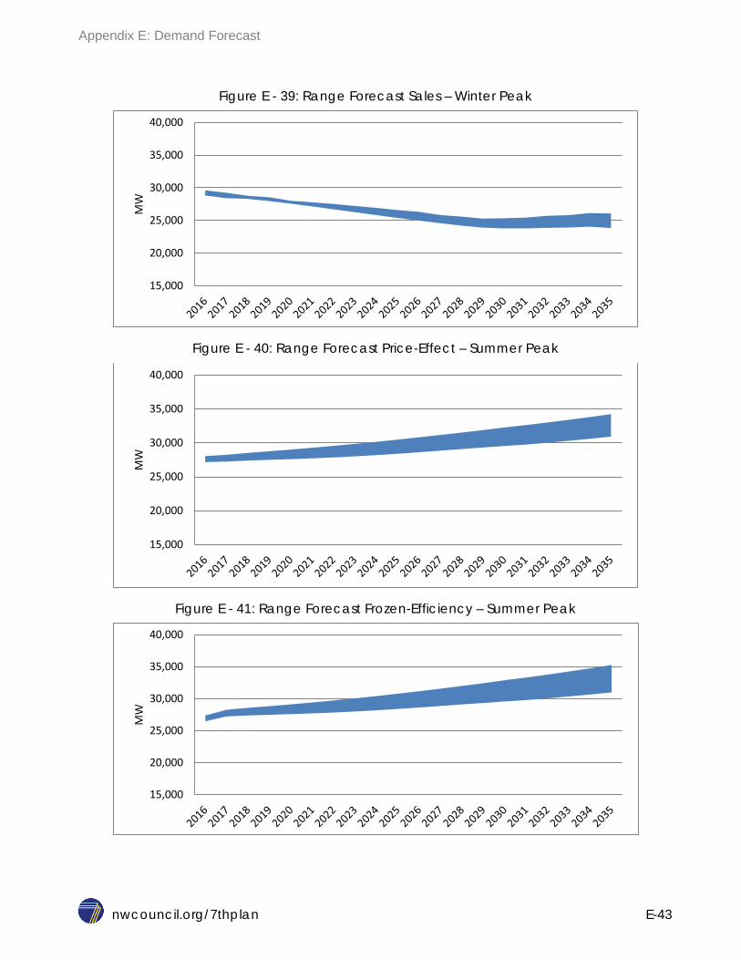
Appendix E: Demand Forecast
nwcouncil.org/7thplan E-43
Figure E - 39: Range Forecast Sales – Winter Peak
Figure E - 40: Range Forecast Price-Effect – Summer Peak
Figure E - 41: Range Forecast Frozen-Efficiency – Summer Peak
15,000
20,000
25,000
30,000
35,000
40,000 M
W
15,000
20,000
25,000
30,000
35,000
40,000
MW
15,000
20,000
25,000
30,000
35,000
40,000
MW
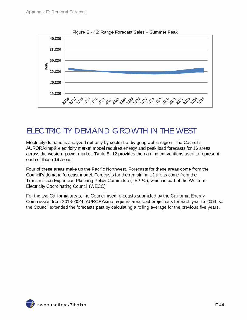
Appendix E: Demand Forecast
nwcouncil.org/7thplan E-44
Figure E - 42: Range Forecast Sales – Summer Peak
ELECTRICITY DEMAND GROWTH IN THE WEST Electricity demand is analyzed not only by sector but by geographic region. The Council’s AURORAxmp® electricity market model requires energy and peak load forecasts for 16 areas across the western power market. Table E -12 provides the naming conventions used to represent each of these 16 areas.
Four of these areas make up the Pacific Northwest. Forecasts for these areas come from the Council’s demand forecast model. Forecasts for the remaining 12 areas come from the Transmission Expansion Planning Policy Committee (TEPPC), which is part of the Western Electricity Coordinating Council (WECC).
For the two California areas, the Council used forecasts submitted by the California Energy Commission from 2013-2024. AURORAxmp requires area load projections for each year to 2053, so the Council extended the forecasts past by calculating a rolling average for the previous five years.
15,000
20,000
25,000
30,000
35,000
40,000
MW

Appendix E: Demand Forecast
nwcouncil.org/7thplan E-45
Table E - 12 - Naming Convention for Aurora Areas
Area Name Short Area Name
Pacific NW Eastside PNWE
California North CANo
California South CASo
British Columbia BC
Idaho South IDS
Montana East MTE
Wyoming WY
Colorado CO
New Mexico NM
Arizona AZ
Utah UT
Nevada North NVNo
Alberta AB
Mexico Baja CA North BajaN
Nevada South NVSo
Pacific NW Westside PNWW
Figure E - 43 shows the 2013 actual and 2035 projected annual energy loads for each area outside Northwest.

Appendix E: Demand Forecast
nwcouncil.org/7thplan E-46
Figure E - 43: 2013 and 2035 Load by AURORA Areas outside NW
Annual average growth rates for demand in the geographic areas outside Northwest are shown in Figure E - 45. This figure shows the projected growth rates for areas that are expected to experience demand increases of less than 1 percent and areas that are forecast to experience demand increases of nearly 2.5 percent per year. The highest projected rates of change are the geographic areas of Alberta, Canada, Baja, Mexico, and Arizona, followed by Wyoming, Utah, and southern and Northern Nevada. Southern and Northern California areas are expected to grow at 0.7 percent per year.
Figure E - 44: 2015-2035 Average Annual Growth Rate for Loads Outside NW
A more detailed dataset on average and peak loads for load areas outside Northwest is provided in the companion workbook from Council’s website. : http://www.nwcouncil.org/energy/powerplan/7/technical
0
5,000
10,000
15,000
20,000
25,000
CANo CASo BC WY CO NM AZ UT NVNo AB BajaN NVSo
Annu
al L
aod
(aM
W)
2013 2035
0.0%
0.5%
1.0%
1.5%
2.0%
2.5%
3.0%
CANo CASo BC WY CO NM AZ UT NVNo AB BajaN NVSo
Aver
age
Annu
al G
row
th R
ate
(%/y
r)

Appendix E: Demand Forecast
nwcouncil.org/7thplan E-47
Figure E - 46 shows the 2013 and projected 2035 peak load by AURORAxmp area, outside the Northwest. The figure demonstrates a wide range in projections of peak demand among geographic areas. It is important to note that these projections are non-coincident (i.e. represent individual utility) peaks.
Figure E - 45: Projected Peak Load by AURORA Area Outside Northwest
SPECIAL FORECAST TOPICS This section describes the impact on electricity demand of custom data centers, embedded data centers, plug-in hybrid and all electric vehicles, and indoor production of cannabis.
Estimating Electricity Demand in Data Centers Background on Trends in Data Center Load
During the development of the Sixth Power Plan, large custom data centers were beginning to enter into the energy picture of Northwest. At that time not much was known about the operations of these data centers and there was uncertainty surrounding their demand for electricity. What attracted these large data centers to the Northwest were: ample, reliable, low electricity prices; low or no tax on construction or operations of the data centers; moderate climate (meaning fewer storms and power interruptions); and good access to communication infrastructure.
What is a Data Center?
"Data center" is a generic term used to describe a number of different types of facilities that house digital electronic equipment for Internet-site hosting, electronic storage and transfer, credit card and financial transaction processing, telecommunications, and other activities that support the growing
0
5,000
10,000
15,000
20,000
25,000
30,000
35,000
40,000
45,000
CANo CASo BC WY CO NM AZ UT NVNo AB BajaN NVSo
Peak
Loa
ds (M
W)
2013
2035

Appendix E: Demand Forecast
nwcouncil.org/7thplan E-48
electronic information-based economy.4 In general, data centers can be categorized into these two main types:
Custom/cloud data centers, such as the Google, Yahoo, and Microsoft facilities in the Grant County PUD and Northern Wasco County PUD. These data centers are typically very large, consisting of thousands of servers and representing a significant demand for power. They are usually sited close to transmission facilities and are typically charged industrial retail rates by their local utility.
Hidden or embedded data centers, like those in business offices, may include a small separate office or closet with a few servers, or larger server facilities with hundreds of servers. These data centers are called “hidden data centers” because they are part of existing commercial businesses. They are usually in urban settings and are typically charged commercial retail electric rates by their local utility.
Table E - 13 touches on some of the characteristics of data centers. The larger custom or cloud data centers are typically in a suburban/rural area, where cheap land is available. The smaller co-location data centers are typically located in metropolitan areas. Difference in size, server concentration, interest and opportunities for efficiency for each data centers type is addressed in table E - 14. Figure E - 47 shows the monthly loads for a few typical large data centers in state of Washington. As can be observed it would take a few years before the data centers utilize their full connected load and the monthly load shapes are not flat.
Table E - 13: Characteristics of Data Centers
4 http://www.gulfcoastchp.org/Markets/Commercial/DataCenters
Example
Approximate Energy Consumption
% of Data Centers in the US
% of Servers in the US
Typical Location
Some of Barriers to Utility Energy Efficiency programs
Opportunity for Energy Efficiency
Enterprise-class/hyper Data Centers
Google, Facebook, Amazon 10-100+ MW 0.3% 28%
non-metro area
secrecy, rapid market change, split incentives, identifying key player, baseline
comprehensive customized offerings/ requires long-term relationship, market movers
Mid-Tire Data Center
Colocators, EasyStreet 10 MW or less 0.4% 15% Metro area
less secrecy, capital constrained, split incentives, baseline and incentive
comprehensive and customized/ requires long-term relationship
Localized Data Center
Hopsital, financial institutions, Government 10-500 KW 2.5% 16% Metro area
Harder to locate, split incentives
Customized/Prescriptive,Training and information on energy efficiency options, long-term relationship
Server closets/Rooms
Small to Mid-size Company 5-10 KW 96% ~40%
business dependent
hard to locate, Small IT resources doing many tasks, IT not core business
Perscriptive program offering
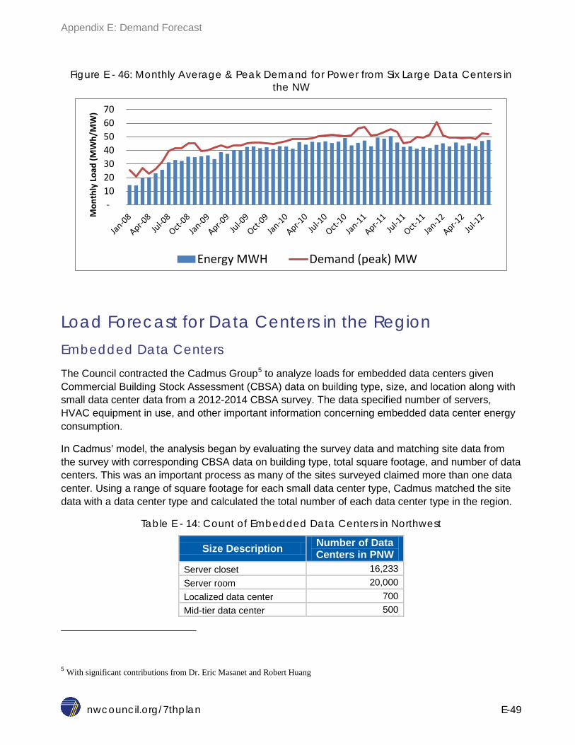
Appendix E: Demand Forecast
nwcouncil.org/7thplan E-49
Figure E - 46: Monthly Average & Peak Demand for Power from Six Large Data Centers in the NW
Load Forecast for Data Centers in the Region Embedded Data Centers
The Council contracted the Cadmus Group5 to analyze loads for embedded data centers given Commercial Building Stock Assessment (CBSA) data on building type, size, and location along with small data center data from a 2012-2014 CBSA survey. The data specified number of servers, HVAC equipment in use, and other important information concerning embedded data center energy consumption.
In Cadmus’ model, the analysis began by evaluating the survey data and matching site data from the survey with corresponding CBSA data on building type, total square footage, and number of data centers. This was an important process as many of the sites surveyed claimed more than one data center. Using a range of square footage for each small data center type, Cadmus matched the site data with a data center type and calculated the total number of each data center type in the region.
Table E - 14: Count of Embedded Data Centers in Northwest
Size Description Number of Data Centers in PNW
Server closet 16,233 Server room 20,000 Localized data center 700 Mid-tier data center 500
5 With significant contributions from Dr. Eric Masanet and Robert Huang
- 10 20 30 40 50 60 70
Mon
thly
Loa
d (M
Wh/
MW
)
Energy MWH Demand (peak) MW

Appendix E: Demand Forecast
nwcouncil.org/7thplan E-50
Cadmus identified the compound annual growth rates (CAGR) for a number of factors contributing to growth in computing and increases in efficiency in the operation of IT equipment. They identified a 20 percent6 annual increase of IP traffic and increases in computations performed by servers,7 computations per watt,8 and watts per device9 for servers, storage, and networking equipment. Applying these growth rates in efficiency and workloads, accounting for IT equipment refresh cycle of 4 years, Cadmus calculated the number of retirements and new IT equipment giving an estimate of total number and energy consumption of IT equipment necessary to meet growing workloads.
Using estimated number of data centers by each space type, from CBSA data, and previously calculated average total IT load by space type,10 Cadmus assumed the percent of energy consumption by IT device type and applied this to the average total IT load to determine the average IT load by device type.11 The average IT load by device was multiplied by the total number of data centers in each space type to calculate total IT load by device (in kilowatts). In order to determine the total load for each data center type in the region, Cadmus calculated infrastructure energy consumption using coefficient of performance12 and PUE - Power usage effectiveness is a measure of how efficiently a data center uses energy; specifically, how much energy is used by the computing equipment (in contrast to cooling and other overhead) for each space type. The total energy consumption by data center type was calculated as the summation of total infrastructure load and total IT load. Table E-15 displays energy consumption by space type and IT device.
Table E - 15: Estimated current data center load by data center type and enduse (aMW)
Enduse Server closet
Server room Localized Mid-tier
Enterprise/ Co locators
Cloud/ Custom Total
Servers 20.4 85.0 8.3 45.7 112.5 158.2 430.2 Storage - - 1.7 9.1 22.5 31.6 65.0
6 Cisco Systems (2014). Visual Networking Index (VNI): The Zettabyte Era—Trends and Analysis. San Jose. http://www.cisco.com/c/en/us/solutions/collateral/service-provider/visual-networking-index-vni/VNI_Hyperconnectivity_WP.html
7Koomey,Jonathan; Berard,Stephen; Sanchez,Marla;Wong,Henry; Stanford University “Implications of Historical Trends in the Electrical Efficiency of Computing” Annals of the History of Computing, IEEE, March 2011 Volume: 33 Issue:3, pages46-54 ISSN:10586180.
Pflueger, J. (2010). Understanding Data Center Energy Intensity: A Dell Technical White Paper. Dell Incorporated. Round Rock, Texas. 8 This rate is derived from Koomey’s Law which states; the number of computations per joule of energy dissipated has been doubling approximately every 1.57 years 9 Watts per device is calculated as the ratio of computations per device to computations per watt 10 This analysis used data on total number of used and unused racks, self reported by small data centers, and a calculated value for UPS power draw per server rack (kW) to make assumptions about total average IT load by space type used in the model to determine total load by space type. 11 Masanet, E., Brown, R.E., Shehabi, A., Koomey, J.G., and B. Nordman (2011). “Estimating the Energy Use and Efficiency Potential of U.S. Data Centers. Proceedings of the IEEE, Volume 99, Number 8
12 'COP = (kW of IT load + kW of cooling electricity)/(kW of cooling electricity)

Appendix E: Demand Forecast
nwcouncil.org/7thplan E-51
Network 1.1 9.4 1.1 6.1 15.0 21.1 53.8 Transformers - 4.7 0.6 3.0 7.5 2.1 17.9
UPS 4.3 18.9 2.2 12.2 15.0 10.5 63.2 Lighting 1.1 1.9 0.2 1.2 3.0 4.2 11.6 Cooling 9.3 33.7 4.3 24.8 50.0 21.1 143.2
Total 36.1 153.7 18.4 102.3 225.5 248.9 784.9
Enterprise and Cloud Data Centers
The Council began its analysis of enterprise and cloud data centers by identifying enterprise data centers within the region and determining through the data centers’ websites, total megawatt capacity, total square footage, and kilowatt per square foot for each facility. From the list of identified enterprise centers in the region and their reported square footage it was estimated that, 75 percent of the total square footage of data center space in Oregon and 94 percent of the square footage in Washington was accounted for by the sample. There are not many data centers in Idaho and Montana. Idaho, Montana, and Washington’s values for total square footage and connected load were left unadjusted due to the large percentage of total square footage accounted for by the sample; Oregon’s square footage was adjusted to account for the missing 25 percent of the population. Based on this analysis, the Council’s preliminary estimate is that enterprise data centers represented between 200-300 megawatts of connected load in the region in 2014.
The same process was repeated with private, very large data centers (Facebook, Google) located in Oregon and Washington (there were no identified or large custom data centers located in Idaho or Montana). The data on connected load was left unadjusted for both Oregon and Washington as a large percentage of the square footage of these data centers in the region was accounted for in the sample. The Council estimated a regional connected load of roughly 250-300 megawatts for cloud data centers in 2014.
These estimates for connected load were applied to the model13,14 developed by Cadmus to determine preliminary estimates of total energy consumption of enterprise and cloud data centers in 2014. The model estimated that roughly 230 average megawatts and 250 average megawatts are consumed by enterprise and cloud data centers, respectively. Figure E - 48 displays preliminary estimates for energy consumption for each data center type in the region for 2014. The Cadmus model, with the addition of the Council’s findings on connected load for enterprise and cloud data centers, estimates regional data center loads of 930 average megawatts in 2014.
13 Connected factors were determined for both enterprise and cloud through research of the industry. A 50% connected factor was applied to the model for enterprise data centers and a 90% connected factor applied to cloud data center connected load estimates 14 It was determined through research on energy consumption in enterprise and cloud data centers that 50% of enterprise data center energy use goes to IT equipment and, in cloud data centers, 80% of energy consumption goes to IT equipment. These two percentages are included in the model to determine average load by data center type.

Appendix E: Demand Forecast
nwcouncil.org/7thplan E-52
Figure E - 47: Estimates for Energy Consumption in 2014 for all Data Centers in the Region
Regional Data Center Energy Consumption 2014-2035 The Cadmus model was used to determine a preliminary load forecast of data centers loads in the region out to 2035 under five scenarios with varying changes in efficiency in both IT equipment and infrastructure systems. The five scenarios are business as usual, best practice adoption, commercial technology adoption, cutting edge technology adoption, and shifting both server closets and server rooms to the cloud. For business as usual (BAU) forecast for data center loads in the region by space type, see Figure E - 49.
Figure E - 48: NWPCC Regional Data Center Energy Use by Space Type under Business as Usual Scenario
From the business as usual (BAU) scenario, which uses baseline power draws for each IT device and infrastructure system (cooling, lighting, transformer, and UPS unit), the Council applies efficiency measures to energy consumption consistently from 2014 through 2035 to estimate the
- 50
100 150 200 250 300
Annu
al C
onsu
mpt
ion
(aM
W) Cooling
Lighting
UPS
Transformers
Network
Storage
Servers
- 200 400 600 800
1,000 1,200 1,400 1,600 1,800 2,000
2014
20
15
2016
20
17
2018
20
19
2020
20
21
2022
20
23
2024
20
25
2026
20
27
2028
20
29
2030
20
31
2032
20
33
2034
20
35
Annu
al L
oad
(aM
W)
Cloud
Enterprise
Mid-tier
Localized
Server room
Server closet

Appendix E: Demand Forecast
nwcouncil.org/7thplan E-53
savings for other scenarios: best practice adoption, commercial technology, cutting edge, and shift to cloud. In the best practice adoption scenario, device reduction ratio of servers increases with assumed increases in virtualization of servers,15 along with increases in the percent of power management and device reduction in storage. This scenario produces significant savings from the BAU scenario with roughly 400 average megawatts of savings in the first year of implementation (2015). Commercial technology scenario assumes increases in percentage of ENERGY STAR® servers in use incrementally until it reaches 100 percent penetration in 2018. In this scenario, infrastructure systems become more efficient with decreases in IT loads. The cutting edge technology adoption scenario assumes storage and network equipment utilization increases with associated decreases in PUE of infrastructure (due to lower IT loads similar to commercial technology adoption). In the final scenario, shift to the cloud, assumes all server closets and rooms shift to the cloud shifting this energy consumption from the regional load from smaller data centers to large custom centers. Figure E – 50 presents the remaining data center load that would results from each of these scenarios.
Figure E - 49: Possible range of loads for embedded data centers
15 Percent of legacy servers goes to 0 as utilization increases
0
100
200
300
400
500
600
700
2014
2015
2016
2017
2018
2019
2020
2021
2022
2023
2024
2025
2026
2027
2028
2029
2030
2031
2032
2033
2034
2035
Annu
al L
oad
(aM
W)
BAU Best practice adoption
Commercial technology adoption Cutting edge technology adoption
Shift closets, rooms to cloud

Appendix E: Demand Forecast
nwcouncil.org/7thplan E-54
Future Trends for Plug-in Hybrid or all Electric Vehicles (EV) Background
Concern for the environment and volatile gasoline prices have created great interest in electric vehicles, both all electric and plug-in hybrids. The most recent data from EPA show that annual sales increased from about 350 vehicles in December 2010 to sales of over 11,000 vehicles in December 2014. This is significant given the financial crisis the US auto industry went through during the recession. The number of EV branded vehicles increased from 2 in 2010 to 23 in 2014. Cumulatively, from 2010 through February of 2015 over 300,000 EVs were sold nationwide. Figure E – 51 shows the number of each brand sold by month over this period.
Figure E - 50: count of EV and PHEV vehicles Nationwide
Although national availability of the electric vehicles has been limited, the Northwest states of Washington and Oregon were among states where electric vehicles were available for purchase. As of July 2015, there were 22,650 EV or PHEV light vehicles in operation in the region. Table E - 16 shows allocation of vehicles by state and type.

Appendix E: Demand Forecast
nwcouncil.org/7thplan E-55
Table E - 16: Allocation of Vehicles by state and type
STATE EV PHEV Grand Total
IDAHO 149 295 444 MONTANA 114 378 492 OREGON 4350 2754 7104 WASHINGTON 10403 4207 14610 Grand Total 15016 7634 22650
The majority of EV purchases have been in the metropolitan areas of Washington and Oregon. The maps shown in Figures E – 52 and E – 53 provide data on the distribution of EVs by county.
Figure E – 51: Electric Vehicles Registered by County in Washington State

Appendix E: Demand Forecast
nwcouncil.org/7thplan E-56
Figure E – 52: Electric Vehicles Registered by County in Oregon State
Potential Effects on Electricity Demand
To analyze the effect of plug-in electric vehicles on electricity demand, three pieces of information are needed: forecast range for number of EVs, forecast of use per vehicle, and trend in efficiency. For estimates on number of EVs, the Council used Q3 HIS-Global Insight forecast of new passenger and light duty vehicles for each state in the Northwest. For forecast of use per vehicle, the Council used results of EV project (a nationally conducted project tracking large number of EV and PHEVs (http://www.theevproject.com/). For the trends in efficiency, the Council used DOE/EIA/AEO 2014 results.
From the EV project tracking large number of EV vehicles, covering over 93 million miles of travel, data indicate that on average 0.26 kilowatt-hours are used to travel one mile. In addition, the average daily distance traveled is between 28 and 38 miles. From the Annual Energy Outlook, the Council used a 2.5 percent improvement in performance of EV from 2015-2035. Combining number of vehicles, use per day, and improvement in performance, the Council estimated the impact of EVs on system load and used hourly load profile for charging events (as part of EV project) shown in Figure E – 54 to estimate peak and off peak impacts.

Appendix E: Demand Forecast
nwcouncil.org/7thplan E-57
Figure E – 53 Load Profile for Electric Vehicle Charging
Average load is projected to increase from the current estimated 10 average megawatts in 2014 to between 160 and 650 average megawatts by 2035. Given hourly pattern of charging, where most of the charging happens at night, off-peak (post midnight) impact on loads is significantly higher, in the 250 to 1200 average megawatt range. Currently, peak period changing is significantly less than off-peak charging. Estimated range for peak is between 7 and 32 megawatts. Table E - 17 below shows range of impact on system average, peak, and off-peak loads.

Appendix E: Demand Forecast
nwcouncil.org/7thplan E-58
Table E - 17: Impact of Electric Vehicle on Northwest Regional Load
Annual Energy aMW
Annual Energy aMW
On Peak MW
On Peak MW
Off Peak MW
Off Peak MW
Low High Low High Low High 2010 0.3 0.3 0.01 0.01 1 1 2011 0.8 0.8 0.04 0.04 1 1 2012 2.5 2.5 0.13 0.13 5 5 2013 5.7 5.7 0.29 0.29 11 11 2014 10.5 12.1 0.53 0.60 20 22 2015 16.0 21.5 0.80 1.08 30 40 2016 21.6 35.2 1.08 1.76 40 65 2017 28.7 54.4 1.44 2.72 53 101 2018 37.1 78.6 1.86 3.93 69 146 2019 46.6 106.8 2.33 5.34 87 199 2020 57.0 138.3 2.85 6.91 106 257 2021 68.3 171.6 3.41 8.58 127 319 2022 80.2 207.0 4.01 10.35 149 385 2023 91.5 244.2 4.57 12.21 170 454 2024 101.9 282.1 5.10 14.11 190 525 2025 111.7 320.7 5.58 16.03 208 596 2026 120.6 359.6 6.03 17.98 224 669 2027 128.5 398.8 6.43 19.94 239 742 2028 135.5 437.5 6.78 21.88 252 814 2029 141.6 475.3 7.08 23.77 263 884 2030 146.6 511.0 7.33 25.55 273 951 2031 150.6 544.1 7.53 27.21 280 1,012 2032 153.7 573.5 7.69 28.67 286 1,067 2033 155.9 598.8 7.80 29.94 290 1,114 2034 157.4 620.4 7.87 31.02 293 1,154 2035 158.2 638.4 7.91 31.92 294 1,187

Appendix E: Demand Forecast
nwcouncil.org/7thplan E-59
Estimating Electricity Demand in Indoor Cannabis Production Background on Cannabis Production and Recent Changes in Cannabis Legislation
A new load to the region emerged in 2014 with the legalization of recreational cannabis use in the state of Washington (under I-502) and legalization in Oregon in November 2014.
Outdoor production of cannabis is far less energy intensive than greenhouse or indoor production; however, producers who choose to grow outdoors are subject to the natural climate and environment which constraints producers to one to two growing cycles a year compared to indoor production which averages 4.7 cycles a year with average cycle duration at 78 days.16 The indoor production of cannabis tends to be energy intensive using high-intensity discharge lamps (e.g. metal halide or high-pressure sodium lamps) for up to twenty four hours a day operating all year. Indoor production is popular for cannabis growing because it allows producers to control every aspect of the plant’s growth, specifically light intensity and spectrum, photoperiod, temperature cycle, nutrients, humidity cycle, CO2 exposure, pruning, leeching, cloning, and the amount of stress the plant experiences.
Estimating the potential future electric loads used for cannabis production is important since the industry is new and magnitude of demand for cannabis that fuels the production is very uncertain. The Council Seventh Power Plan forecast a regional load of 180 to 300 average megawatts will be used in indoor cannabis production by 2035. This estimate is calculated from estimates for cannabis demand in each state in the region.
Baseline for Indoor Production
Although costs of indoor production far exceed that of outdoor due to lighting and other start-up costs, the benefits of indoor production, specifically higher yield and cannabinoid content, mean many cannabis producers are located indoors. Of recently approved cannabis producers in Washington state, 49 percent of total production is located inside. Of tier 2 producers, the largest number of licenses held by approved producers in Washington, 32 percent are located indoors.17 Through phone surveys with approved producers in Washington, and a review of literature concerned with economic and energy impacts of legalization of cannabis in Washington and Colorado,18 the Council was able to establish a baseline estimate of indoor production.
Many indoor production facilities are separated by rooms which are dedicated to one period of the plant’s growing cycle. Plants begin in vegetation, or “veg” rooms where plants are in the early to mid-
16 Mills, Evan. Energy up in Smoke: The Carbon Footprint of Indoor Cannabis Production. University of California. April 15, 2011. Table 1, pg. 4. http://evan-mills.com/energy-associates/Indoor.html 17 Washington’s application for production of recreational cannabis are designated by allowable canopy size in square footage and producers are given a tier size, 1 being the smallest and 3 being the largest. 18 Primary source of information on indoor production RAND and BOTEC

Appendix E: Demand Forecast
nwcouncil.org/7thplan E-60
stages of growth. Plants in this room are kept under 1,000 watt metal halide lamps with a possible addition of 500-1200 watt T5 fluorescents or 42 watt CFLs. Hours of light use range between 18 hours on with 6 hour off periods, or lights can stay on for 24 hours. Vegetation rooms on average have 2.5 to 8 plants per lamp, yet vary widely in square footage and number of plants due to facility size and strain type. Producers maintain a humidity level of 50 to 55 percent and temperature set point of 78 to 80 degrees Fahrenheit. Temperature and humidity are maintained through the use of combination of mini-split air conditioning (AC) units and heat pumps. There is typically a 3 ton AC unit for every 250 square foot of floor area. Many producers used AC units to controlled humidity levels so they do not need a separate dehumidifier system.
When the plants begin to mature, they are moved to a flowering room where lighting conditions are changed while humidity levels and temperature set-point are very similar to the vegetation room (humidity level of 45-55 percent with temperature set at 82 degrees with lights on to 70 degrees with lights off). Lighting typically used in this room is more intense than vegetation rooms with producers using 1,000 watt high pressure sodium lamps with fewer plants per lamp (roughly 2.5 plants per lamp) and lighting times of 12 hours on and 12 off.
Both vegetation and flower rooms require ventilation due to the heat produced by HID lighting; this results in the use of hoods with ventilation fans or centrifugal fans ranging from 800-2,000 cubic feet per minute (2 fans per 400-500 sq ft). Despite the heat produced by lighting, about 20 percent of surveyed indoor producers in Washington keep rooms entirely sealed and reported no use of ventilation. Based on research on indoor production, growers may use some form of CO2 in production in order to shorten plant cycles and increase yield; however, only 2 of the 16 survey respondents used some form of CO2 enrichment in their facility (with reported 1250 ppm).
Load Forecast for Indoor Cannabis Production
The Council estimated the electricity used in the region in the production of cannabis two ways. The “supply side” estimate was compared to the “demand side” to confirm results. The demand-side approach considers estimated total cannabis demand by state, and uses baseline measurements for kilowatt-hour of energy required per kilogram of product produced to derive total average megawatts needed for production to meet demand. The demand-side will be discussed first, and then two supply side approaches will be considered in order to form a preliminary range for cannabis load.
Load Forecast Using Demand Method
In estimating demand, the Council utilized data provided by the National Survey on Drug Use and Health19 (NSDUH) through its “restricted use data analysis system” on the percentages of previous month use by age category in each state in the region. Applying these percentages to population data provided by IHS-Global Insight in a 2014 analysis, population estimates for past month users by age group in each state were estimated. An organization in Colorado20 provided data on share of
19 Substance Abuse and Mental Health Services Administration. (2002–2011). 2002-2011 NSDUH State Estimates of Substance Use and Mental Disorders. (Multiple data files). http://www.samhsa.gov/data/NSDUH.aspx 20 Light, Miles K. Orens, Adam. Lewandowski,Brian. Pickton, Tom. The Marijuana Policy Group. Market Size and Demand for Marijuana in Colorado: Prepared for the Colorado Department of Revenue. Colorado Department of Revenue. 2014.

Appendix E: Demand Forecast
nwcouncil.org/7thplan E-61
past month users in varying use amount categories corresponding to use amounts in grams. These data were applied to population data to get low, central, and high use amounts by varying use frequencies in the past month. The Council calculated a preliminary estimate for cannabis demanded in Washington of 103 to 160 metric tons in 2014 and a range of 215 to 345 metric tons in 2035. Each state’s preliminary estimates for cannabis demand are shown in Figure E - 55.
Figure E - 54: Preliminary Estimates for Cannabis in Metric Tons by State
Using a list of approved producers provided by Washington State Liquor Control Board, in which the production option is specified (outdoor, indoor, etc.), the Council calculated the percentage of approved producers by production type. Taking the percentages of production option (3 percent of producers chose greenhouse only production, 56 percent of producers chose indoor production, etc.), and using the preliminary estimate for demand in metric tons in Washington (range of 103 to 160 metric tons) the Council estimated the amount of kilograms of cannabis produced in each production option. These are reported in Table E – 18.
0
50
100
150
200
250
300
2014 2015 2020 2025 2030 2035
Idaho
Montana
Oregon
Washington
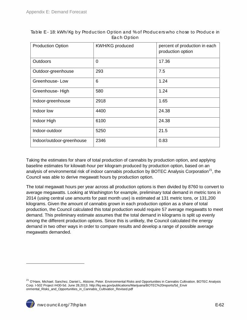
Appendix E: Demand Forecast
nwcouncil.org/7thplan E-62
Table E - 18: kWh/Kg by Production Option and % of Producers who chose to Produce in Each Option
Production Option KWH/KG produced percent of production in each production option
Outdoors 0 17.36
Outdoor-greenhouse 293 7.5
Greenhouse- Low 6 1.24
Greenhouse- High 580 1.24
Indoor-greenhouse 2918 1.65
Indoor low 4400 24.38
Indoor High 6100 24.38
Indoor-outdoor 5250 21.5
Indoor/outdoor-greenhouse 2346 0.83
Taking the estimates for share of total production of cannabis by production option, and applying baseline estimates for kilowatt-hour per kilogram produced by production option, based on an analysis of environmental risk of indoor cannabis production by BOTEC Analysis Corporation21, the Council was able to derive megawatt hours by production option.
The total megawatt hours per year across all production options is then divided by 8760 to convert to average megawatts. Looking at Washington for example, preliminary total demand in metric tons in 2014 (using central use amounts for past month use) is estimated at 131 metric tons, or 131,200 kilograms. Given the amount of cannabis grown in each production option as a share of total production, the Council calculated this total production would require 57 average megawatts to meet demand. This preliminary estimate assumes that the total demand in kilograms is split up evenly among the different production options. Since this is unlikely, the Council calculated the energy demand in two other ways in order to compare results and develop a range of possible average megawatts demanded.
21 O’Hare, Michael. Sanchez, Daniel L. Alstone, Peter. Environmental Risks and Opportunities in Cannabis Cultivation. BOTEC Analysis Corp. I-502 Project #430-5d. June 28,2013. http://liq.wa.gov/publications/Marijuana/BOTEC%20reports/5d_Envir onmental_Risks_and_Opportunities_in_Cannabis_Cultivation_Revised.pdf

Appendix E: Demand Forecast
nwcouncil.org/7thplan E-63
Load Forecast Using Two Supply Side Methods
The first supply side approach considered uses the total allowable square footage for cannabis production in Washington and a metric for kilowatt-hour per square foot per year, based on a review of indoor production facilities in Colorado, to estimate annual energy demand. The caveat of this approach is that it assumes total production is done indoors with all facilities consisting of the same square footage, which is an unrealistic measurement and will result in an overestimate of demand. However, this approach provides a maximum expected demand if the previous assumptions are met. Taking total allowable square footage in Washington, 2,000,000 square feet, and using a measurement22 of 448 kWh/sq.ft/year, the Council calculated a preliminary estimate of total energy demand.
2,000,000 𝑠𝑞.𝑓𝑡.∗ 448 𝑘𝑤ℎ𝑠𝑞𝑓𝑡
= 896,000,000 𝑘𝑊ℎ/𝑦𝑒𝑎𝑟
24 ℎ𝑜𝑢𝑟𝑠 𝑜𝑛 ∗ 365 𝑑𝑎𝑦𝑠 = 8,760 ℎ𝑜𝑢𝑟𝑠
896,000,000 𝑘𝑊ℎ8,760 ℎ𝑜𝑢𝑟𝑠= 102,283 𝑘𝑊
102,283 𝑘𝑊1000
= 102 𝑎𝑀𝑊
The Council believes 102 average megawatts of demand 2014 in Washington’s indoor cannabis production to be an upper bound of electricity consumption for reasons stated earlier.
The second supply side approach suggests that a more accurate preliminary estimate can be reached by taking a previously calculated metric for kilowatt-hours per square foot combined with primary source data on facility size as a percentage of total allowable square footage. By using data on the number of producers in smaller facilities, and therefore using less energy in lighting and HVAC, a more realistic estimate for total demand can be developed.
From the Washington list of 121 approved producers and reported total square footage, 10 percent of the square footage is occupied by tier 1 producers, 30 percent by tier 2 and 60 percent by tier 3. Given the share of total square footage held by each tier, the Council estimated total square footage by tier size. Using a list of indoor producers by square footage and connected load (provided by a utility in Washington), the Council calculated a regression coefficient of 0.04 kilowatt per square foot. The square footage in each tier size was multiplied by the 0.04 kilowatts per square foot and then by the typical hours of lighting in the different stages of plant growth to estimate annual energy use. The result of this calculation provided an estimate for current electricity use for cannabis production of 80 average megawatts. This preliminary estimate of demand lies between the two previous calculations. Table E – 19 shows the estimated consumption by tier.
22 kWh/kg/cycle comes from a facility reviewed by Xcel energy in Colorado. The Council used Xcel Energy’s estimate for kWh/kg/cycle and converted it to an annual measurement assuming 4 cycles a year.
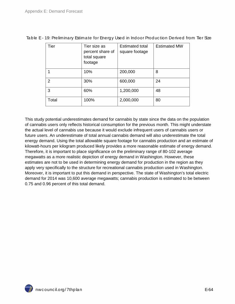
Appendix E: Demand Forecast
nwcouncil.org/7thplan E-64
Table E - 19: Preliminary Estimate for Energy Used in Indoor Production Derived from Tier Size
This study potential underestimates demand for cannabis by state since the data on the population of cannabis users only reflects historical consumption for the previous month. This might understate the actual level of cannabis use because it would exclude infrequent users of cannabis users or future users. An underestimate of total annual cannabis demand will also underestimate the total energy demand. Using the total allowable square footage for cannabis production and an estimate of kilowatt-hours per kilogram produced likely provides a more reasonable estimate of energy demand. Therefore, it is important to place significance on the preliminary range of 80-102 average megawatts as a more realistic depiction of energy demand in Washington. However, these estimates are not to be used in determining energy demand for production in the region as they apply very specifically to the structure for recreational cannabis production used in Washington. Moreover, it is important to put this demand in perspective. The state of Washington’s total electric demand for 2014 was 10,600 average megawatts; cannabis production is estimated to be between 0.75 and 0.96 percent of this total demand.
Tier Tier size as percent share of total square footage
Estimated total square footage
Estimated MW
1 10% 200,000 8
2 30% 600,000 24
3 60% 1,200,000 48
Total 100% 2,000,000 80

Seventh Northwest Conservation and Electric Power Plan
nwcouncil.org/7thplan F-1
APPENDIX F: EFFECT OF FEDERAL APPLIANCE EFFICIENCY STANDARDS
Contents Summary of Results ................................................................................................................... 3 Introduction ................................................................................................................................ 4 Methodology .............................................................................................................................. 8
Improvement in Distribution Transformers .............................................................................. 8 Dynamic Standards ................................................................................................................ 8
List of Figures and Tables
Figure F - 1: Programmatic and Non-programmatic Factors Impacting Energy Savings ............. 3 Table F - 1: Direct Impact of Federal Standards in Northwest Loads (aMW) ............................. 3 Figure F - 2: Year by Year Direct Impact of Federal Standards ................................................. 4 Table F - 2: Direct Impact of Federal Standards in All Sectors (aMW) ....................................... 5 Table F - 3: Year by Year Direct Impact of Federal Standards in Residential sector (aMW) ...... 6 Table F - 4: Year by Year Direct Impact of Federal Standards in Commercial Sector (aMW) .... 7 Table F - 5: Year by Year Direct Impact of Federal Standards in Industrial and other Sector (aMW) ........................................................................................................................................ 7 Table F - 6: Impact of Dynamic Standards on Average Annual Growth Rate of Load ................. 9

Appendix F: Effect of Federal Appliance Efficiency Standards
nwcouncil.org/7thplan F-2
This appendix describes the steps used to estimate the impact of federal appliance standards on electricity demand in the Pacific Northwest for 2015-2035. The federal appliance standards reduce the amount of electricity needed in the future, but these reductions are not well-reflected in the econometric models used by many of the region’s forecasters. This appendix is intended to help utility forecasters, energy-efficiency planners, and others in the region concerned with accounting for energy-efficiency achievements.
Typically, the Council’s forecast of future loads starts with an estimate of current efficiency levels of enduse devices. For example, current loads for the refrigeration enduse in the residential sector depend on the current level of energy consumption of the refrigerators. The future forecast for refrigeration loads is dependent on the consumption of future refrigerators. Future efficiency depends on the relationship between cost of the refrigerators, efficiency of refrigerators, and consumer preferences. Also impacting future consumption are the standards enacted, at federal or state level, to remove less efficient refrigerator models from the market. A combination of push and pull effects influence consumers’ choices.
Utility efficiency programs build on the existing baseline for each measure and incentivize consumer selections toward higher efficiency devices (Pull Effect). Federal and state standards, on the other hand, push for increasing the minimum efficiency of the devices. Combination of the two strategies pushes the low efficiency measures out and helps pull-in higher efficiency measures.
Implementation of standards helps reduce future loads more economically and more equitably than conservation programs. Typically, standards are applicable to 100 percent of consumer base, whereas the conservation programs will only eventually reach an upper limit of 85 percent of consumer base. The standards are also more equitable in that they do not require ratepayer funding for incentivizing conservation measures.
Figure F - 1 shows the multiple mechanisms used to achieve energy conservation. Starting with a baseline of energy consumption at end use and technology level, the program activities push energy conservation to a higher level. Market transformation activities then further enhance the energy conservation initiatives on an upstream basis. The codes and standards play the role of keeping the less efficiency technologies out of the consumer’s hand. The combination of programmatic initiatives and standards also cause market induced (not incentivized) efficiency that consumers partake on their own. The result is a cooperative mechanism through for which codes and standards truncate the less efficient options from a given market, while the programmatic initiatives push the more efficient (above baseline) into the market.

Appendix F: Effect of Federal Appliance Efficiency Standards
nwcouncil.org/7thplan F-3
Figure F - 1: Programmatic and Non-programmatic Factors Impacting Energy Savings
SUMMARY OF RESULTS The Council estimates that the federal efficiency standards on appliances used in residential, commercial, and industrial sectors, adopted since the preparation of its Sixth Power Plan, will reduce system loads in the Pacific Northwest by more than 1,264 average megawatts between 2012 and 2035. The standards are estimated to reduce winter peak loads by over 2,100 megawatts by 2035.
Table F - 1 and Figure F - 2 present the sector-level and sector and end-use-level load reductions for the starting and ending period of analysis.
Table F - 1: Direct Impact of Federal Standards in Northwest Loads (aMW)
2015 2035
Residential 41 614
Commercial 25 467
Industrial 17 163
Transportation 0 11
Street lighting 1 8
Total Direct Impact 83 1,264

Appendix F: Effect of Federal Appliance Efficiency Standards
nwcouncil.org/7thplan F-4
Figure F - 2: Year by Year Direct Impact of Federal Standards
INTRODUCTION The U.S. federal government’s policies on energy efficiency have developed over decades, beginning with the Energy Policy and Conservation Act of 1975, which called for energy efficiency targets, followed by the National Appliance Energy Conservation Act of 1987, which established minimum efficiency standards for a number of household appliances. The Energy Policy Act of 1992, and the Energy Independence and Security Act of 2007 (EISA) expanded the equipment subject to efficiency standards.
The standard-setting process followed by the U.S. Department of Energy requires that standards be reviewed at least once every six years from their effective date, and that they be set at levels to achieve the maximum improvement in energy efficiency that is "technically feasible and economically justified." The Energy Policy and Conservation Act directs the U.S. Department of Energy to consider seven factors in its analysis when determining whether a potential standard is economically justified:
1. Economic impact on consumers and manufacturers 2. Lifetime operating cost savings compared to increased product cost 3. Total projected energy savings over at least one lifetime of the product 4. Impact on product utility or performance 5. Impact of any lessening of competition 6. Need for national energy efficiency 7. Other factors the Secretary considers relevant
0
200
400
600
800
1000
1200
1400
2012
20
13
2014
20
15
2016
20
17
2018
20
19
2020
20
21
2022
20
23
2024
20
25
2026
20
27
2028
20
29
2030
20
31
2032
20
33
2034
20
35
Aver
age
MW
Streetlighting
Transportation
Industrial
Commercial
Residential

Appendix F: Effect of Federal Appliance Efficiency Standards
nwcouncil.org/7thplan F-5
Of these factors, maintaining consumer choice and quality of service has often been an issue. A study1 by the American Council for an Energy-Efficient Economy and the Appliance Standards Awareness Project analyzed the effect of federal efficiency standards on 10 residential, commercial, and lighting products. The study found that performance was maintained and in many cases improved, and that manufacturers offered new features in the products. Price declined or stayed the same in five out of the nine products for which data were available, and the price increases of the other four products were more than offset by the savings in electricity bills.
Using the Council’s Seventh Power Plan’s medium forecast of households, square footage of commercial building stock, load growth in industrial, street lighting, transportation sectors, and appliance stocks, the federal appliance standards’ impact on the 2015 appliance stock is estimated to reduce electricity demand by 83 aMW. This analysis has incorporated updated appliance saturations based on the Residential Building Stock Assessment 2012/2013, Commercial Building Stock Assessment 2013/2014, and updated regional economic and demographic forecasts. A majority of these standards savings are from the residential sector.
Sector level impacts by 2015 and 2035 are shown in Table F - 2. Residential sector impacts by end use are shown in Table F - 3. Commercial sector impacts by end use are shown in Table F - 4. Industrial and other sector impacts by end use are shown in Table F - 5.
Table F - 2: Direct Impact of Federal Standards in All Sectors (aMW)
Sector 2015 2035 Residential 41 614 Commercial 25 467 Industrial 17 163 Transportation 0 11 Street lighting 1 8 Total Direct Impact 83 1,264
1 Joanna Mauer, Andrew DeLaski, Steven Nadel, Anthony Fryer, and Rachel Young, “Better Appliances: An Analysis of Performance, Features, and Price as Efficiency Has Improved,” ACEEE Research Report # 132, May 2013. http://www.aceee.org/research-report/a132
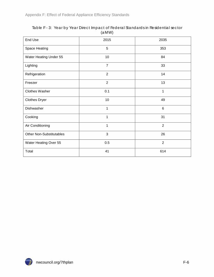
Appendix F: Effect of Federal Appliance Efficiency Standards
nwcouncil.org/7thplan F-6
Table F - 3: Year by Year Direct Impact of Federal Standards in Residential sector (aMW)
End Use 2015 2035
Space Heating 5 353
Water Heating Under 55 10 84
Lighting 7 33
Refrigeration 2 14
Freezer 2 13
Clothes Washer 0.1 1
Clothes Dryer 10 49
Dishwasher 1 6
Cooking 1 31
Air Conditioning 1 2
Other Non-Substitutables 3 26
Water Heating Over 55 0.5 2
Total 41 614

Appendix F: Effect of Federal Appliance Efficiency Standards
nwcouncil.org/7thplan F-7
Table F - 4: Year by Year Direct Impact of Federal Standards in Commercial Sector (aMW)
End Use 2015 2035
Space Heating 1 13
Water Heating 2 20
Other Substitutables 0 15
Refrigeration 3 185
Lighting 11 110
Air Conditioning 5 62
Other Non-Substitutables 2 62
Total 25 467
Table F - 5: Year by Year Direct Impact of Federal Standards in Industrial and other Sector (aMW)
2015 2035
Process Heat 2 18
Motors 7 70
Other Subs 2 24
Miscellaneous 5 52
Total Industrial 17 163
Total Transportation sector* 0.1 11
Total Street lighting and pumping ** 1 8
*Includes Electric vehicles and public transportation, **- includes fresh water and waste water treatment facilities.
Federal efficiency standards also reduce peak loads. Each appliance makes its own unique contribution to peak load, so that efficiency improvements to those appliances have unique impacts on peak loads. The Council’s analysis used data from the End-Use Load and Consumption Assessment Program (ELCAP), conducted by Bonneville from 1986 to 1989 as well as the recent Residential Building Stock Assessment (RBSA) metering study conducted in 2012-2014, to estimate the effects of efficiency improvements on power system peak loads.

Appendix F: Effect of Federal Appliance Efficiency Standards
nwcouncil.org/7thplan F-8
One of the findings from the recent RBSA study was that the many enduses are less “peaky” than earlier findings from ELCAP.
By 2035, winter peak loads are estimated to be about 10 percent lower as a result of standards. The baseline peak is estimated to be about 34,000 megawatts; appliance standards lower this peak load to about 31,000 megawatts.
METHODOLOGY
The Council’s Seventh Plan used a frozen efficiency forecast as the basis for evaluating resource needs in the future. It assumes that baseline energy consumptions of specified equipment and structures remain at fixed levels over the forecast period. These fixed levels are commonly set at current practice at the time the forecast is made. The Council has used the frozen efficiency concept in its forecasting since its First Power Plan in 1983, avoiding the possibility of double counting efficiency improvements.2
The frozen efficiency forecast, in addition to reflecting current practice, also reflects future improvements in efficiencies from known standards. For example, the federal lighting standards from EISA 2007, which take effect from 2013 to 2020, were included in the plan’s frozen efficiency forecast.
Improvement in Distribution Transformers One of the standards that impact all end-uses is for distribution transformers. The Council has used the analysis conducted for EIA/AEO 2014 by Navigant Consulting to estimate the potential reduction in loads due to more efficient distribution transformers. The analysis includes dry-type low voltage distribution transformers, medium voltage dry-type distribution transformers for industrial processes, and liquid filled distribution (LFD) transformers. LFD transformers are all medium voltage with well over 90 percent of shipments serving utilities and the remainder serving industrial processes. To simulate impact of these standards, the Council increased the efficiency of distribution transformers by about 2 percent cumulatively during 2015 and 2035. The average transmission and distribution (T&D) losses during 1995-2013 is estimated at about 10.5 percent. Overtime, the Council has assumed that the efficiency of distribution system to improve from this standard, reducing the T&D losses to closer to 8.6 percent. For more details on this standard see pages the report “analysis and representation of Miscellaneous Electric Loads in NEMS” December 2013.
Dynamic Standards DOE is required by law to renew and reevaluate existing and new standards every sixth year. The Council has attempted to model the impact of such renewal of standards in a scenario called Dynamic Standards. The Council’s analysis has shown that impact of federal standards would keep the loads flat if the existing standards are renewed and improved by 10 percent 2 This could occur if a conventional forecast included efficiency improvements (lowering resource requirements) and planners also counted those improvements as part of the energy efficiency potential (estimated based on current practice) available to meet future loads.

Appendix F: Effect of Federal Appliance Efficiency Standards
nwcouncil.org/7thplan F-9
every six years during 2015-2035. Table F - 6 below shows the impact of Dynamic Standards. The load growth rate declines from about 0.8 percent in the base case to 0.13 percent.
Table F - 6: Impact of Dynamic Standards on Average Annual Growth Rate of Load
2015-2035 Base case Dynamic Standard
Peak (MW) 0.60% 0.03%
Annual Average (aMW) 0.80% 0.13%
Low Load Hours (aMW) 0.90% 0.19%
The primary caveat to this analysis is that there are a vast and growing number of standards at various stages of implementation. In this appendix, the Council has presented its best estimate of the impact of these standards as the Seventh Plan was being developed. However, there are more technologies and standards that are scheduled for implementation, so estimates shown should be treated as minimum impacts. As more standards are finalized future load growth is further reduced.
For a more complete listing of all federal standards, please see Chapter 12 Conservation Resources.
Seventh Northwest Conservation and Electric Power Plan
nwcouncil.org/7thplan G-1
APPENDIX G: CONSERVATION RESOURCES AND DIRECT APPLICATION RENEWABLES
Contents Overview .................................................................................................................................... 4 General Conservation Resource Methodology ........................................................................... 5
Baseline ................................................................................................................................. 8 Units ................................................................................................................................... 8
Technical Potential ................................................................................................................. 8 Technical Achievable Potential ..............................................................................................10 Cost and Benefits of Conservation Resources .......................................................................11
Calculating Levelized Cost .................................................................................................11 Cost of Conservation .........................................................................................................12 Financial Input Assumptions ..............................................................................................13 Benefits of Conservation ....................................................................................................15 Value of Conservation with Respect to Time ......................................................................17
Cost-Effectiveness Analysis Methodology .................................................................................19 Decision Rules for Modeling Conservation Resource Acquisition in the Regional Portfolio Model .................................................................................................................................20 Method for Determining the Cost-Effectiveness Limit for Conservation ..............................21
Supply Curve Workbook Structure ............................................................................................29 Note of Caution about B/C Ratio ............................................................................................31
Residential Sector .....................................................................................................................31 Measure Bundles ...................................................................................................................32 Overview of Methods .............................................................................................................34
Physical Units ....................................................................................................................34 Baseline Characteristics ....................................................................................................34 Measure Applicability .........................................................................................................35 Measure Achievability ........................................................................................................35
Guide to the Residential Conservation Workbooks ................................................................35 Commercial Sector ...................................................................................................................37
Measure Bundles ...................................................................................................................38 Overview of Methods .............................................................................................................41
Physical Units ....................................................................................................................41 Baseline Characteristics ....................................................................................................42 Measure Applicability .........................................................................................................42 Measure Achievability ........................................................................................................43
Guide to the Commercial Conservation Workbooks ...............................................................43 Industrial Sector ........................................................................................................................45
Measure Bundles ...................................................................................................................46

Appendix G: Conservation Resources and Direct Application Renewables
nwcouncil.org/7thplan G-2
Overview of Methods .............................................................................................................47 Physical Units ....................................................................................................................47 Baseline Characteristics ....................................................................................................48 Measure Applicability .........................................................................................................49 Measure Achievability ........................................................................................................49
Guide to the Industrial Sector Workbooks and Data ..............................................................49 Agricultural Sector .....................................................................................................................50
Measure Bundles ...................................................................................................................50 Overview of Methods .............................................................................................................50
Physical Units ....................................................................................................................51 Baseline Characteristics ....................................................................................................51 Measure Applicability and Measure Achievability ...............................................................51
Guide to the Agriculture Conservation Workbooks .................................................................51 Distribution System ...................................................................................................................52
Measure Bundles ...................................................................................................................52 Overview of Methods .............................................................................................................53
Physical Units ....................................................................................................................53 Baseline Characteristics ....................................................................................................53 Measure Applicability .........................................................................................................53 Measure Achievability ........................................................................................................53
Guide to the Distribution Efficiency Workbooks .....................................................................53 Distributed Photovoltaics ...........................................................................................................54
Measure Bundles ...................................................................................................................54 Overview of Methods .............................................................................................................55
Physical Units ....................................................................................................................55 Baseline Characteristics ....................................................................................................56 Measure Applicability and Achievability..............................................................................56 Measure Costs ...................................................................................................................57 Daily and Seasonal Shape and Capacity Contribution .......................................................58
Guide to the Distributed PV Workbooks .................................................................................59
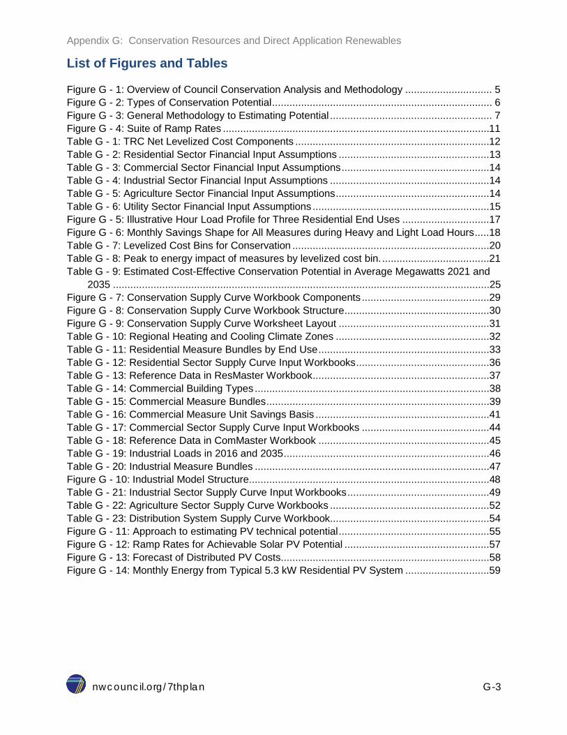
Appendix G: Conservation Resources and Direct Application Renewables
nwcouncil.org/7thplan G-3
List of Figures and Tables Figure G - 1: Overview of Council Conservation Analysis and Methodology .............................. 5 Figure G - 2: Types of Conservation Potential ............................................................................ 6 Figure G - 3: General Methodology to Estimating Potential ........................................................ 7 Figure G - 4: Suite of Ramp Rates ............................................................................................11 Table G - 1: TRC Net Levelized Cost Components ...................................................................12 Table G - 2: Residential Sector Financial Input Assumptions ....................................................13 Table G - 3: Commercial Sector Financial Input Assumptions ...................................................14 Table G - 4: Industrial Sector Financial Input Assumptions .......................................................14 Table G - 5: Agriculture Sector Financial Input Assumptions .....................................................14 Table G - 6: Utility Sector Financial Input Assumptions .............................................................15 Figure G - 5: Illustrative Hour Load Profile for Three Residential End Uses ..............................17 Figure G - 6: Monthly Savings Shape for All Measures during Heavy and Light Load Hours .....18 Table G - 7: Levelized Cost Bins for Conservation ....................................................................20 Table G - 8: Peak to energy impact of measures by levelized cost bin. .....................................21 Table G - 9: Estimated Cost-Effective Conservation Potential in Average Megawatts 2021 and
2035 ..................................................................................................................................25 Figure G - 7: Conservation Supply Curve Workbook Components ............................................29 Figure G - 8: Conservation Supply Curve Workbook Structure ..................................................30 Figure G - 9: Conservation Supply Curve Worksheet Layout ....................................................31 Table G - 10: Regional Heating and Cooling Climate Zones .....................................................32 Table G - 11: Residential Measure Bundles by End Use ...........................................................33 Table G - 12: Residential Sector Supply Curve Input Workbooks ..............................................36 Table G - 13: Reference Data in ResMaster Workbook .............................................................37 Table G - 14: Commercial Building Types .................................................................................38 Table G - 15: Commercial Measure Bundles .............................................................................39 Table G - 16: Commercial Measure Unit Savings Basis ............................................................41 Table G - 17: Commercial Sector Supply Curve Input Workbooks ............................................44 Table G - 18: Reference Data in ComMaster Workbook ...........................................................45 Table G - 19: Industrial Loads in 2016 and 2035 .......................................................................46 Table G - 20: Industrial Measure Bundles .................................................................................47 Figure G - 10: Industrial Model Structure ...................................................................................48 Table G - 21: Industrial Sector Supply Curve Input Workbooks .................................................49 Table G - 22: Agriculture Sector Supply Curve Workbooks .......................................................52 Table G - 23: Distribution System Supply Curve Workbook.......................................................54 Figure G - 11: Approach to estimating PV technical potential ....................................................55 Figure G - 12: Ramp Rates for Achievable Solar PV Potential ..................................................57 Figure G - 13: Forecast of Distributed PV Costs ........................................................................58 Figure G - 14: Monthly Energy from Typical 5.3 kW Residential PV System .............................59

Appendix G: Conservation Resources and Direct Application Renewables
nwcouncil.org/7thplan G-4
OVERVIEW This appendix provides an overview of the general methodology used by the Council for estimating the conservation resource potential in the region and describes the major sources of information used to prepare that analysis. It also provides a description of the spreadsheet workbooks containing the detailed input assumptions and specific source data used for each of the measures in the Council’s conservation supply curves. The workbooks are available on the Council’s Seventh Power Plan web site http://www.nwcouncil.org/energy/powerplan/7/technical.
The Council structures this work by examining many conservation measures. A conservation “measure” is any device or method that results in electricity savings compared with its baseline. The Council estimates costs and savings for over 1,600 measure permutations.1 These costs and savings, coupled with savings shape over time, capacity impacts, and estimates of the possible pace of deployment, are used to develop supply curves of conservation potential available by year. The supply curves represent the amount, daily and seasonal shape, and capacity characteristics of conservation available at different cost levels by year. Costs are expressed as TRC (Total Resource Cost) net levelized costs, in 2012 dollars, so they can be compared to the costs of power purchases and the costs of new resource development.2 The Council uses an in-house model called ProCost to calculate measure-level TRC net levelized cost, estimate the hourly, daily and seasonal savings, and identify capacity impact of efficiency measures. The levelized cost and savings potential amount, by season and year, and the capacity impacts are inputs to the Regional Portfolio Model.
The Regional Portfolio Model determines the amount of energy efficiency to be developed to achieve least-cost and least-risk adequate electric system for the region. Findings from the Regional Portfolio Model include year-by-year conservation development goals, expressed in average megawatts of energy, to achieve a least-cost and least-risk system. Regional Portfolio Model findings are also used to establish conservation cost-effectiveness methodologies to guide conservation program development. The methodology for cost-effectiveness is based on a benefit-to-cost ratio rather than a levelized cost. The benefit-to-cost ratio provides a means to assure that both the shaped energy and capacity savings of the measures are taken into account.
Figure G - 1 describes the overall process. The first tier of Figure G - 1 includes the development of inputs for the conservation assessment which is the subject of this appendix.
1 A measure permutation includes different applications and different efficiencies for a given measure. For example, a 1.5 GPM showerhead in single family homes with electric water heating is a unique permutation for the low-flow showerhead measure. Other measure permutations would change the segment (multifamily, manufactured), the flow-rate of the showerhead (1.0 GPM), or the water heater type (heat pump water heater). 2 “TRC Net Levelized Cost” is computed based on all costs minus all benefits regardless of which sponsor incurs the cost or accrues the benefits. TRC Net Levelized Cost includes all applicable costs and all benefits. In addition to energy system costs and benefits, TRC Net Levelized Cost includes non-energy, other-fuel, O&M, periodic-replacement and risk-mitigation benefits and costs. TRC Net Levelized Cost corresponds to TRC B/C ratios with regard to the costs and benefits included. Benefits are subtracted from costs, and then levelized over the life of the program.
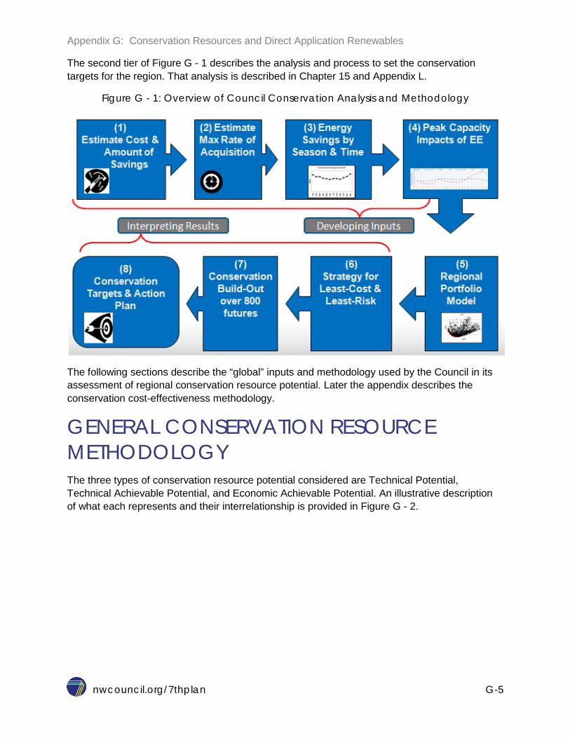
Appendix G: Conservation Resources and Direct Application Renewables
nwcouncil.org/7thplan G-5
The second tier of Figure G - 1 describes the analysis and process to set the conservation targets for the region. That analysis is described in Chapter 15 and Appendix L.
Figure G - 1: Overview of Council Conservation Analysis and Methodology
The following sections describe the “global” inputs and methodology used by the Council in its assessment of regional conservation resource potential. Later the appendix describes the conservation cost-effectiveness methodology.
GENERAL CONSERVATION RESOURCE METHODOLOGY The three types of conservation resource potential considered are Technical Potential, Technical Achievable Potential, and Economic Achievable Potential. An illustrative description of what each represents and their interrelationship is provided in Figure G - 2.
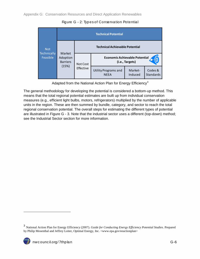
Appendix G: Conservation Resources and Direct Application Renewables
nwcouncil.org/7thplan G-6
Figure G - 2: Types of Conservation Potential
Adapted from the National Action Plan for Energy Efficiency3
The general methodology for developing the potential is considered a bottom-up method. This means that the total regional potential estimates are built up from individual conservation measures (e.g., efficient light bulbs, motors, refrigerators) multiplied by the number of applicable units in the region. These are then summed by bundle, category, and sector to reach the total regional conservation potential. The overall steps for estimating the different types of potential are illustrated in Figure G - 3. Note that the industrial sector uses a different (top-down) method; see the Industrial Sector section for more information.
3 National Action Plan for Energy Efficiency (2007). Guide for Conducting Energy Efficiency Potential Studies. Prepared by Philip Mosenthal and Jeffrey Loiter, Optimal Energy, Inc. <www.epa.gov/eeactionplan>
Not Technically
Feasible
Technical Potential
Market Adoption Barriers
(15%)
Technical Achievable Potential
Not Cost Effective
Economic Achievable Potential(i.e., Targets)
Utility Programs and NEEA
Market-Induced
Codes & Standards

Appendix G: Conservation Resources and Direct Application Renewables
nwcouncil.org/7thplan G-7
Figure G - 3: General Methodology to Estimating Potential
Each of these components will be discussed further below.

Appendix G: Conservation Resources and Direct Application Renewables
nwcouncil.org/7thplan G-8
Baseline The “baseline” refers to the conditions of the electricity-using buildings, systems, and devices at the start of the plan. For conservation, the baseline is what the energy efficiency is measured against. The baseline estimate is a critical factor in determining both energy savings and forecast energy demand. The Council uses a frozen efficiency baseline forecast described in Chapter 7. Estimates of current market conditions and characteristics of the building stock come from several sources. Key among these are the residential, commercial, and industrial stock assessments completed by the Northwest Energy Efficiency Alliance (NEEA), selected studies from utilities, Bonneville, Energy Trust of Oregon, and other sources.
For new and replacement equipment, baseline conditions are the more efficient of either (1) minimum applicable code or standard or (2) market conditions at the start of the planning period. State building codes and federal and state standards for equipment are continually being upgraded. The baseline assumptions codes and standards used in the Seventh Power Plan are those that were adopted at the end of 2014, with few exceptions. Some of these include standards that were adopted before the end of 2014, but with effective dates that occur in the future. For such codes or standards, both savings estimates and the demand forecast reflect the effective dates of adopted standards. If current market practice is more efficient than code, baselines are generally estimated using the average efficiency as typically taken from available sales data. Lacking sales data, other sources are used such as retail stocking data (such as the California Energy Commission appliance database), ENERGY STAR market share data, distributor sales data, and store shelf surveys. The Council estimates current market practice as of the beginning of 2016. Cost data are from utility program data, US DOE National Impact Assessment workbooks, or on-line retail stores. There is a baseline assumption for each measure in the Council analysis. These baseline assumptions are described in the measure workbooks.
Units
Coupled with the baseline efficiencies are the counts of buildings/systems/devices. In all cases, the number of units is tied to the demand forecast. In development of the forecast (see Chapter 7), the Council projects the total number of units (e.g. households, by state and segment, or commercial square feet, by state and segment) over the 20-year planning horizon. These quantities, multiplied by the saturations and electric fuel shares, give the total number of units available. For example, the number of refrigerators is equal to the number of households times the average number of refrigerators per home. Within the sector-specific sections below, more details are provided on the sources for number of units.
Technical Potential Technical potential is the amount of conservation that is technically feasible. It considers conservation measures and the number of these measures that could physically be installed, without regard to achievability or cost. It can be viewed as the upper limit of what conservation potential is available.

Appendix G: Conservation Resources and Direct Application Renewables
nwcouncil.org/7thplan G-9
A conservation “measure” is any device or method that results in electricity savings compared with its baseline. The Power Act defines conservation as “any reduction in electric power consumption as a result of increases in the efficiency of energy use, production, or distribution”.4 For a measure to constitute conservation under the Act, it has to meet both parts of the definition. That is, the measure must reduce electric power consumption and the reduced consumption must result from an increase in the efficiency of energy use, production, or distribution. A measure that does just one or the other – for example, reduce electricity consumption but not through an efficiency increase – does not qualify as “conservation” under the Act.
Measures are identified from the range of measures currently in utility programs, as well as a broad search of utility potential assessments, emerging technology research, and input from local, regional, and national experts. Once the measures are identified, Council staff seeks to identify adequate and reliable savings and cost data. Costs and savings are based both on engineering estimates, as well as estimates based on results from the operation of existing programs. Note that although the Council included a wide-ranging list of measures, no conservation assessment can include all efficiency measures that could be installed. Some measures were passed over due to lack of data or resources at the time of the supply curve development. The Council believes these omissions do not significantly impact results. A list of known missing measures is provided as part of the discussion about each sector. Also, as described in Chapter 12, there are additional measures only included in the emerging technology scenario, as the Council does not yet consider them currently available and reliable. If a measure is not in the Seventh Power Plan, this does not preclude program administrators from providing incentives for such a measure.
The efficiency measures are grouped into three bundles: new, natural replacement, and retrofit applications. There are three reasons to distinguish these application modes. First, costs and savings can be different by application mode. Second, in the case of new and natural replacement, the available stock for the measure depends on the forecast of new additions and replacement rate for equipment. These opportunities are tracked separately over course of the forecast period and limit the annual availability of conservation opportunities. Third, the Council’s portfolio model treats new and natural replacement applications as lost-opportunity measures that can only be captured at the time of construction or natural replacement.
Measure costs, savings, applicability, and achievability estimates are identified separately for each of the new, natural replacement, and retrofit application modes. The Council analyzes measure costs and savings on an incremental basis. Measure cost is the incremental cost over what would be done absent the measure or program. The same is true for savings. Incremental measure costs and savings can be different depending on the application mode. For example, incremental costs of high performance windows in a new application only include the additional cost of the windows required by code. In a retrofit application, the labor cost of removing and replacing the existing window are added to the measure cost.
4 Northwest Power Act,§3(3), 94 Stat. 2698.

Appendix G: Conservation Resources and Direct Application Renewables
nwcouncil.org/7thplan G-10
Measure applicability reflects two major components: technical applicability and measure saturation. First is the technical applicability of a measure. Technical applicability includes what fraction of the stock the measure applies to. Technical applicability can be composed of several factors. These include the fraction of stock that the measure applies to, overlap with mutually exclusive measures, and the existing saturation of the measure. Existing measure saturation reflects the fraction of the applicable stock that has already adopted the measure and for which savings estimates do not apply. When the baseline is equivalent to the average market conditions, then the measure saturation is set to zero.
Technical Achievable Potential The Council assumes that only a portion of the technically available conservation can be achieved. Ultimate achievability factors are limited to 85 percent of the technically available conservation over the twenty-year forecast period.5 In addition to a limit of 85 percent, the Council estimates near-term achievable penetration rates for bundles of conservation measures. For these estimates, conservation measures are bundled based on the characteristics of the measures and consideration of the likely delivery mechanisms. In the Seventh Power Plan, the Council uses a suite of typical ramp rates to reflect penetration rates, illustrated in Figure G - 4. For example, measures involving emerging technology might start out at low penetration rates and gradually increase to 85 percent penetration. Measures suitable for implementation by a building code or a federal equipment standard might increase rapidly to 85 percent penetration in new buildings and major remodels. Measures requiring new delivery mechanisms might ramp up slowly. Simple measures with well-established delivery channels, like efficient showerheads, might take only half a dozen years to fully implement. Whereas retrofit measures in complex markets might take 20 years to reach full penetration. The Council also considers region wide conservation program accomplishments when developing these ramp rates to help align early year potential with recent historic accomplishments. Assumptions for the ramp rates applied to each measure are detailed in the conservation supply curve workbooks described by sector below.
5 See http://www.nwcouncil.org/reports/2007/2007-13/ for more information on the source of 85%.
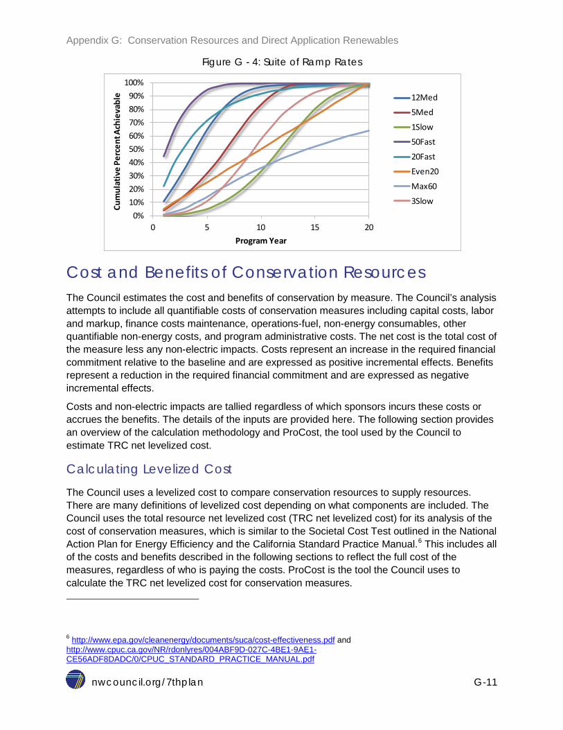
Appendix G: Conservation Resources and Direct Application Renewables
nwcouncil.org/7thplan G-11
Figure G - 4: Suite of Ramp Rates
Cost and Benefits of Conservation Resources The Council estimates the cost and benefits of conservation by measure. The Council’s analysis attempts to include all quantifiable costs of conservation measures including capital costs, labor and markup, finance costs maintenance, operations-fuel, non-energy consumables, other quantifiable non-energy costs, and program administrative costs. The net cost is the total cost of the measure less any non-electric impacts. Costs represent an increase in the required financial commitment relative to the baseline and are expressed as positive incremental effects. Benefits represent a reduction in the required financial commitment and are expressed as negative incremental effects.
Costs and non-electric impacts are tallied regardless of which sponsors incurs these costs or accrues the benefits. The details of the inputs are provided here. The following section provides an overview of the calculation methodology and ProCost, the tool used by the Council to estimate TRC net levelized cost.
Calculating Levelized Cost
The Council uses a levelized cost to compare conservation resources to supply resources. There are many definitions of levelized cost depending on what components are included. The Council uses the total resource net levelized cost (TRC net levelized cost) for its analysis of the cost of conservation measures, which is similar to the Societal Cost Test outlined in the National Action Plan for Energy Efficiency and the California Standard Practice Manual.6 This includes all of the costs and benefits described in the following sections to reflect the full cost of the measures, regardless of who is paying the costs. ProCost is the tool the Council uses to calculate the TRC net levelized cost for conservation measures.
6 http://www.epa.gov/cleanenergy/documents/suca/cost-effectiveness.pdf and http://www.cpuc.ca.gov/NR/rdonlyres/004ABF9D-027C-4BE1-9AE1-CE56ADF8DADC/0/CPUC_STANDARD_PRACTICE_MANUAL.pdf
0%10%20%30%40%50%60%70%80%90%
100%
0 5 10 15 20
Cum
ulat
ive
Perc
ent A
chie
vabl
e
Program Year
12Med
5Med
1Slow
50Fast
20Fast
Even20
Max60
3Slow

Appendix G: Conservation Resources and Direct Application Renewables
nwcouncil.org/7thplan G-12
The primary components of the TRC net levelized cost are the net present value (NPV) of the measure costs divided by the annual savings of the measure. Economic costs and benefits are converted to present value costs and benefits based the financing costs, sponsor cost shares, and discount rates. ProCost uses standard capital recovery factors and present value (PV) factors to calculate PV costs and benefits. Finance costs use sponsor-specific interest rates and terms as assigned by user input to calculate PV of capital costs of measures. Annual costs and benefits that are not financed are counted in the years they occur and discounted to present values using standard present value factors and the global discount rate of 4 percent used in all Council analysis for the Seventh Plan.
ProCost sums all of the present value costs and nets out benefits. This net present value is then amortized over the life of the program (20 years) using standard capital recovery factors and the discount rate. The resulting annual “levelized” cost is divided by the discounted annual energy savings adjusted for transmission and distribution line losses to produce a levelized cost per unit energy saved in dollars per kWh.
The TRC net levelized costs are all costs minus all benefits regardless of which sponsor incurs the cost or accrues the benefits. In addition to energy system costs and benefits, TRC net levelized cost includes non-energy, program administration, other-fuel, O&M, periodic-replacement benefits and costs. The ten percent Regional Act Credit is taken into consideration in the Regional Portfolio Model and thus not included in the TRC net levelized costs uses in the supply curve inputs. The costs and benefits included in the Seventh Power Plan are summarized on Table G - 1. Each of these parameters is discussed in the following sections.
Table G - 1: TRC Net Levelized Cost Components
Costs Included Benefits Netted Out Capital & Labor Deferred T & D Expansion
Annual O&M Regional Act Credit* Program Administration Deferred Generation Capacity Investment** Periodic Replacement Avoided Periodic Replacement
Other Fuel Costs Other Fuel Benefits Non-Energy Impacts Non-Energy Impacts
*The 10 percent advantage for conservation in the Northwest Power Act is accounted for when comparing conservation and other resources in the RPM rather than in the levelized cost of conservation. ** The value of deferred generation capacity is determined as part of the RPM analysis and is not included as part of the levelized cost input to the RPM analysis.
Cost of Conservation
The cost of conservation, as described above, is based on the incremental cost of the measure compared to the baseline case. The Council also includes a programmatic administration cost, approximated at 20 percent of the incremental cost. In addition to those up-front costs, a measure may have on-going operation and maintenance (O&M) costs (or benefits) compared to the baseline. For example, a heat pump water heater has maintenance costs to clean filters and discharge condensate compared to an electric resistance water heater. There may also be periodic replacement costs (or benefits) compared to the baseline. An example of the periodic replacement cost is the replacement of system component that was not present in the baseline system, like a compressor in a heat pump heating system that replaces an electric baseboard heating system. There may also be other fuel costs, such as additional gas heating required
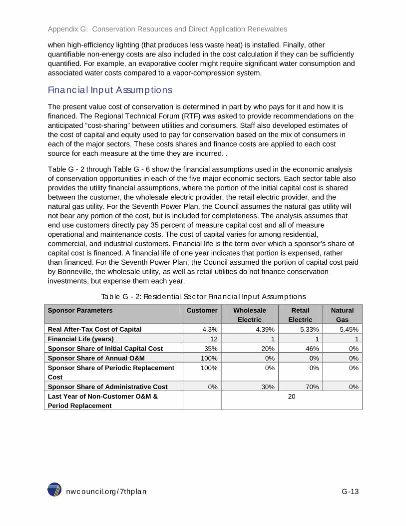
Appendix G: Conservation Resources and Direct Application Renewables
nwcouncil.org/7thplan G-13
when high-efficiency lighting (that produces less waste heat) is installed. Finally, other quantifiable non-energy costs are also included in the cost calculation if they can be sufficiently quantified. For example, an evaporative cooler might require significant water consumption and associated water costs compared to a vapor-compression system.
Financial Input Assumptions
The present value cost of conservation is determined in part by who pays for it and how it is financed. The Regional Technical Forum (RTF) was asked to provide recommendations on the anticipated “cost-sharing” between utilities and consumers. Staff also developed estimates of the cost of capital and equity used to pay for conservation based on the mix of consumers in each of the major sectors. These costs shares and finance costs are applied to each cost source for each measure at the time they are incurred. .
Table G - 2 through Table G - 6 show the financial assumptions used in the economic analysis of conservation opportunities in each of the five major economic sectors. Each sector table also provides the utility financial assumptions, where the portion of the initial capital cost is shared between the customer, the wholesale electric provider, the retail electric provider, and the natural gas utility. For the Seventh Power Plan, the Council assumes the natural gas utility will not bear any portion of the cost, but is included for completeness. The analysis assumes that end use customers directly pay 35 percent of measure capital cost and all of measure operational and maintenance costs. The cost of capital varies for among residential, commercial, and industrial customers. Financial life is the term over which a sponsor’s share of capital cost is financed. A financial life of one year indicates that portion is expensed, rather than financed. For the Seventh Power Plan, the Council assumed the portion of capital cost paid by Bonneville, the wholesale utility, as well as retail utilities do not finance conservation investments, but expense them each year.
Table G - 2: Residential Sector Financial Input Assumptions
Sponsor Parameters Customer Wholesale Electric
Retail Electric
Natural Gas
Real After-Tax Cost of Capital 4.3% 4.39% 5.33% 5.45% Financial Life (years) 12 1 1 1 Sponsor Share of Initial Capital Cost 35% 20% 46% 0% Sponsor Share of Annual O&M 100% 0% 0% 0% Sponsor Share of Periodic Replacement Cost
100% 0% 0% 0%
Sponsor Share of Administrative Cost 0% 30% 70% 0% Last Year of Non-Customer O&M & Period Replacement
20

Appendix G: Conservation Resources and Direct Application Renewables
nwcouncil.org/7thplan G-14
Table G - 3: Commercial Sector Financial Input Assumptions
Sponsor Parameters Customer Wholesale Electric
Retail Electric
Natural Gas
Real After-Tax Cost of Capital 6.8% 4.39% 5.33% 5.45% Financial Life (years) 12 1 1 1 Sponsor Share of Initial Capital Cost 35% 20% 46% 0% Sponsor Share of Annual O&M 100% 0% 0% 0% Sponsor Share of Periodic Replacement Cost
100% 0% 0% 0%
Sponsor Share of Admin Cost 0% 30% 70% 0% Last Year of Non-Customer O&M & Period Replacement
20
Table G - 4: Industrial Sector Financial Input Assumptions
Sponsor Parameters Customer Wholesale Electric
Retail Electric
Natural Gas
Real After-Tax Cost of Capital 8.5% 4.39% 5.33% 5.45% Financial Life (years) 12 1 1 1 Sponsor Share of Initial Capital Cost 35% 20% 46% 0% Sponsor Share of Annual O&M 100% 0% 0% 0% Sponsor Share of Periodic Replacement Cost
100% 0% 0% 0%
Sponsor Share of Admin Cost 0% 30% 70% 0% Last Year of Non-Customer O&M & Period Replacement
20
Table G - 5: Agriculture Sector Financial Input Assumptions
Sponsor Parameters Customer Wholesale Electric
Retail Electric
Natural Gas
Real After-Tax Cost of Capital 6.8% 4.39% 5.33% 5.45% Financial Life (years) 12 1 1 1 Sponsor Share of Initial Capital Cost 35% 20% 46% 0% Sponsor Share of Annual O&M 100% 0% 0% 0% Sponsor Share of Periodic Replacement Cost
100% 0% 0% 0%
Sponsor Share of Admin Cost 0% 30% 70% 0% Last Year of Non-Customer O&M & Period Replacement
20
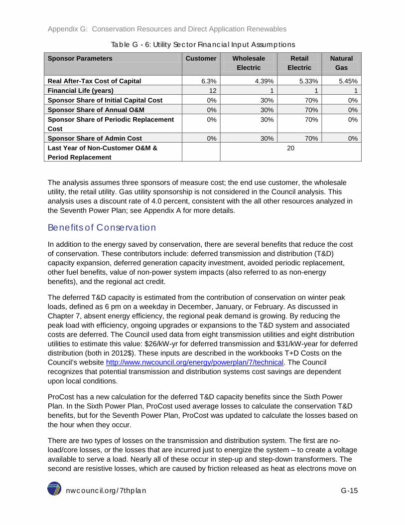
Appendix G: Conservation Resources and Direct Application Renewables
nwcouncil.org/7thplan G-15
Table G - 6: Utility Sector Financial Input Assumptions
Sponsor Parameters Customer Wholesale Electric
Retail Electric
Natural Gas
Real After-Tax Cost of Capital 6.3% 4.39% 5.33% 5.45% Financial Life (years) 12 1 1 1 Sponsor Share of Initial Capital Cost 0% 30% 70% 0% Sponsor Share of Annual O&M 0% 30% 70% 0% Sponsor Share of Periodic Replacement Cost
0% 30% 70% 0%
Sponsor Share of Admin Cost 0% 30% 70% 0% Last Year of Non-Customer O&M & Period Replacement
20
The analysis assumes three sponsors of measure cost; the end use customer, the wholesale utility, the retail utility. Gas utility sponsorship is not considered in the Council analysis. This analysis uses a discount rate of 4.0 percent, consistent with the all other resources analyzed in the Seventh Power Plan; see Appendix A for more details.
Benefits of Conservation
In addition to the energy saved by conservation, there are several benefits that reduce the cost of conservation. These contributors include: deferred transmission and distribution (T&D) capacity expansion, deferred generation capacity investment, avoided periodic replacement, other fuel benefits, value of non-power system impacts (also referred to as non-energy benefits), and the regional act credit.
The deferred T&D capacity is estimated from the contribution of conservation on winter peak loads, defined as 6 pm on a weekday in December, January, or February. As discussed in Chapter 7, absent energy efficiency, the regional peak demand is growing. By reducing the peak load with efficiency, ongoing upgrades or expansions to the T&D system and associated costs are deferred. The Council used data from eight transmission utilities and eight distribution utilities to estimate this value: $26/kW-yr for deferred transmission and $31/kW-year for deferred distribution (both in 2012$). These inputs are described in the workbooks T+D Costs on the Council’s website http://www.nwcouncil.org/energy/powerplan/7/technical. The Council recognizes that potential transmission and distribution systems cost savings are dependent upon local conditions.
ProCost has a new calculation for the deferred T&D capacity benefits since the Sixth Power Plan. In the Sixth Power Plan, ProCost used average losses to calculate the conservation T&D benefits, but for the Seventh Power Plan, ProCost was updated to calculate the losses based on the hour when they occur.
There are two types of losses on the transmission and distribution system. The first are no-load/core losses, or the losses that are incurred just to energize the system – to create a voltage available to serve a load. Nearly all of these occur in step-up and step-down transformers. The second are resistive losses, which are caused by friction released as heat as electrons move on

Appendix G: Conservation Resources and Direct Application Renewables
nwcouncil.org/7thplan G-16
increasingly crowded lines and transformers. Typically, about 25 percent of the average annual losses are no-load or core losses, and about 75 percent are resistive losses.
Losses increase significantly during peak periods. ProCost uses the formula for the resistive losses, I2R, where “I” is the amperage (current) on any particular transformer or distribution line, and “R” is the resistance of the wires through which that current flows. While the “R” is generally constant through the year, since utilities use the same wires and transformers all year long, the “I” is directly a function of the demand that customers place on the utility. Thus, resistive losses increase with the square of the current, meaning losses increase as load increases. Depending on the system load shape, the percentage of generation that is “lost” before it reaches loads is typically at least twice as high as the average annual losses on the system. During the highest critical peak hours (perhaps 5-25 hours per year) when the system is under stress, the losses may be four to six times higher than the average.
ProCost uses the system load shape and the conservation measure load shape to calculate the impact of the measure on system losses, accounting for both the core and resistive losses. 7
Conservation measures also have a deferred generation capacity value, though the economic value of this is derived from analysis of resource strategies in the Regional Portfolio Model rather than fixed as an input. As such, the economic value of deferred generation capacity was set to zero for the RPM inputs. Instead, the derived economic value of deferred generation capacity is captured in the determination of the plan conservation goals and for setting cost-effectiveness levels for conservation measures and programs. Measure cost-effectiveness methodology is described in the section below titled “Determining the Cost-Effectiveness Limit for Conservation”.
The other benefits of conservation included in the levelized cost calculation include the periodic replacement, other fuel, and quantifiable non-power system impacts. An example of the periodic replacement benefit is a high-efficiency LED light bulb that has a significantly longer life than a baseline halogen bulb. As such, by installing an LED that has a 12-year measure life, the user avoids replacing the halogen bulb five times (every two years).
The other fuel benefits are savings in natural gas or heating oil from, for example, increased insulation levels. The homeowner who has air conditioning and a gas furnace will save electricity in reduced cooling usage as well as saving gas from reduced heating usage by adding ceiling insulation.
In addition, the Council includes the value of quantifiable non-power system impacts. For example, by installing an efficient clothes washer, the homeowner will use less water than the baseline. The value of this water reduction is included as a benefit in the net levelized cost calculation.
Finally, the Northwest Power Act directs the Council and Bonneville to give conservation a 10 percent cost advantage over sources of electric generation.8 The Council does this by
7 Overall conservation avoids line losses that range between 7 and 8 percent depending on the load shape of each measure’s savings.
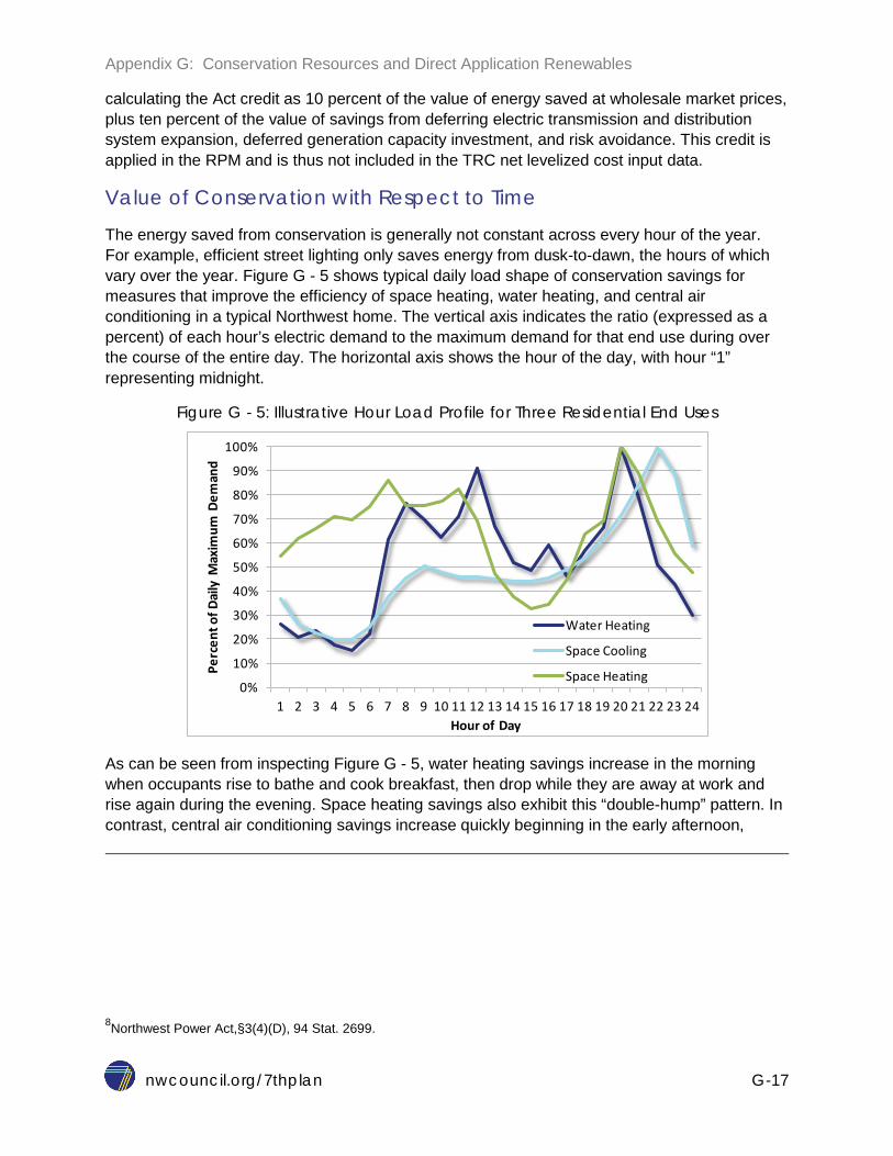
Appendix G: Conservation Resources and Direct Application Renewables
nwcouncil.org/7thplan G-17
calculating the Act credit as 10 percent of the value of energy saved at wholesale market prices, plus ten percent of the value of savings from deferring electric transmission and distribution system expansion, deferred generation capacity investment, and risk avoidance. This credit is applied in the RPM and is thus not included in the TRC net levelized cost input data.
Value of Conservation with Respect to Time
The energy saved from conservation is generally not constant across every hour of the year. For example, efficient street lighting only saves energy from dusk-to-dawn, the hours of which vary over the year. Figure G - 5 shows typical daily load shape of conservation savings for measures that improve the efficiency of space heating, water heating, and central air conditioning in a typical Northwest home. The vertical axis indicates the ratio (expressed as a percent) of each hour’s electric demand to the maximum demand for that end use during over the course of the entire day. The horizontal axis shows the hour of the day, with hour “1” representing midnight.
Figure G - 5: Illustrative Hour Load Profile for Three Residential End Uses
As can be seen from inspecting Figure G - 5, water heating savings increase in the morning when occupants rise to bathe and cook breakfast, then drop while they are away at work and rise again during the evening. Space heating savings also exhibit this “double-hump” pattern. In contrast, central air conditioning savings increase quickly beginning in the early afternoon,
8Northwest Power Act,§3(4)(D), 94 Stat. 2699.
0%
10%
20%
30%
40%
50%
60%
70%
80%
90%
100%
1 2 3 4 5 6 7 8 9 10 11 12 13 14 15 16 17 18 19 20 21 22 23 24
Perc
ent o
f Dai
ly M
axim
um D
eman
d
Hour of Day
Water Heating
Space Cooling
Space Heating

Appendix G: Conservation Resources and Direct Application Renewables
nwcouncil.org/7thplan G-18
peaking in late afternoon and decline again as the evening progresses and outside temperatures drop. Measure savings can also vary seasonally and by day of the week. As the price of electricity varies by day and by season, the value of the conservation will also vary, depending on its savings shape.
The shape of the savings for the complete set of conservation measures in the supply curve during heavy and light load hours is provided in Figure G - 6. As is shown, the energy savings are greater during the winter season than summer, in large part due to significant savings from conversion of electric resistance heating to more efficient heat pump technologies and increased use of lighting during the winter period. As such, the conservation measures have a greater impact on winter peak load requirements than summer peak requirements. Winter peak hours are defined as 6pm on a weekday in December, January, or February. Summer peak hours are defined as 6pm on a weekday in July or August. The peak capacity factor9 varied from around 1.2 in summer to around 2.0 in winter, indicating that conservation measures have a fairly significant impact on peak loads, particularly in the winter. Of course each individual conservation measure analyzed by the Council have a unique shape, which will have an effect on its value as a resource option and on measure cost-effectiveness.
Figure G - 6: Monthly Savings Shape for All Measures during Heavy and Light Load Hours
9 Capacity factor in this context is defined as the peak savings in megawatts divided by the annual energy savings in average megawatts.
0%
1%
2%
3%
4%
5%
6%
7%
Pere
cent
of A
nnua
l Ene
rgy
Savi
ngs
Month
Heavy Load HoursLight Load Hours
Appendix G: Conservation Resources and Direct Application Renewables
nwcouncil.org/7thplan G-19
COST-EFFECTIVENESS ANALYSIS METHODOLOGY The Council uses a multi-step process to evaluate the cost and amount of conservation to be developed for a least-cost and least risk resource strategy. Conservation supply curves are constructed based on cost and savings available from over 1,600 conservation measure permutations across the residential, commercial, industrial, agriculture, and the electric utility system sectors. The conservation supply curves, annual deployment limitations, and the seasonal and time of day availability of conservation data are provided as inputs to the RPM. Data on the cost and availability of generating resource options are also provided to the RPM. The RPM tests plans for the development of conservation and generation resources across 800 different futures. The RPM analysis produces strategies for conservation and generation resource development that have lowest cost and lowest economic risk outcomes for the region. The Council then considers the RPM conservation strategies, along with practical considerations, to develop near-term conservation targets and actions as well as cost-effectiveness guidance for near-term conservation program decisions. The process is outlined in Figure G - 1 above.
As with all other resources, the Council uses the RPM to determine how much conservation is cost-effective to develop.10 The RPM compares resources, including conservation on a “generic” level. That is, it does not model a specific combined cycle gas or wind project nor does it model specific conservation measures or programs. Run time constraints limit the number of conservation programs the RPM can consider. The RPM cannot consider individual programs for every measure and every specific load shape, and perform a measure-specific benefit-cost ratio for each sub-component of conservation. Therefore, the Council simplifies the set of conservation measures available to the portfolio model. In the case of conservation, the model uses two separate supply curves.
These two supply curves, one for retrofit resources and a second for lost opportunity resources, depict the amount of savings achievable at varying levelized costs. The lost opportunity measures incorporate those that are new or natural replacement applications. The estimates of costs and savings in the supply curves incorporate line loss savings, the value of deferred distribution capacity expansion, and the non-energy costs and benefits of the savings, as discussed above. The available savings are also allocated to heavy and light-load time periods to reflect the time-based value of savings and savings impact on capacity needs.
10 A full explanation of how the RPM arrives at the cost-effective amount of conservation is described in Appendix L in the section entitled “The Sources of Increased Conservation”.

Appendix G: Conservation Resources and Direct Application Renewables
nwcouncil.org/7thplan G-20
Decision Rules for Modeling Conservation Resource Acquisition in the Regional Portfolio Model
The reason the RPM uses separate lost-opportunity and retrofit supply curves is that if a lost opportunity conservation resource is not acquired when it is available, it cannot be acquired later (e.g., after the building is constructed) or cannot be cost-effectively acquired later (e.g., the cost of revisiting a home makes adding an increment of ceiling insulation non-cost effective). Thus, the maximum amount of lost opportunity resources is limited annually based on the new construction and equipment turnover. Since retrofit conservation resources do not have this restricted “window of opportunity,” the maximum amount of conservation is limited by the total long-term potential. Deferring the purchase of high-cost conservation resources to periods when market costs are high reduces cost and risk. That is, a portfolio management strategy that acquires high-cost conservation resources early results in higher cost and risk than a strategy that defers their acquisition to periods in future when market prices are higher. If market prices are expected to increase over time, the value acquiring high-cost conservation resource is less in the near-term than in the long term.
The RPM models conservation resources using fourteen11 annual supply curve bins that represent the quantity of technically achievable conservation available each year from 2016 through 2035 at levelized cost. The supply curves are differentiated by levelized cost bin and by retrofit versus lost opportunity resources. The conservation in these cost bins carry with them the shape and capacity characteristics of the combined set of measures in the cost bin. The cost bins, used for both resources are in Table G - 7, along with the average cost and total amount of conservation potential. Note, the RPM can select a portion of conservation within a bin.
Table G - 7: Levelized Cost Bins for Conservation
Bin Cost Range (2012$/MWh)
Average Levelized Cost (2012$/MWh)
Maximum Conservation (aMW)
LO Retrofit LO Retrofit Total 1 <$20 -$21 -$32 959 883 1,841 2 $20-50 36 36 1,802 1,598 3,400 3 $50-80 64 65 2,220 1,857 4,078 4 $80-110 92 94 2,317 2,055 4,372 5 $110-140 126 125 2,506 2,079 4,585 6 $140-170 156 160 2,621 2,129 4,750 7 >$170 580 410 2,818 2,271 5,088
In addition to the numbers presented in the above table there are 38 aMW of potential from short-term lighting savings (pre-2020), all available at less than $20 per megawatt-hour. This potential accounts for savings between the current baseline and the 2020 lighting standard of 45
11 Seven cost bins for the two resource types (retrofit and lost opportunity)

Appendix G: Conservation Resources and Direct Application Renewables
nwcouncil.org/7thplan G-21
lumens per watt. Since these savings do not persist past 2020, they are inputted separately from the other conservation measures (they are inputted as a contract purchase).
The amount of conservation resources technically achievable each year increases based on the assumption that programs are able to capture an ever larger share of the available potential over time, as determined by the ramp rates provided in Figure G - 4. The RPM can acquire these technically achievable resources each year up to the quantity it determines to be cost-effective over the full planning period and across the 800 futures tested by the RPM. However, the ramp rate for the measures in a specific cost bin are based on the year in which that bin is deployed in the resource strategy. For example, if bin 4 is deployed in 2020, the achievability for that bin will begin at a low value, based on the first year of ramp rate acquisition, or Program Year 1 in Figure G - 4.
The final conservation input into RPM is the capacity value of the savings. Given each conservation measure has an associated savings shape (see Figure G - 5), the contribution of savings during peak hours differs by this shape. For each measure category, the Council calculated the peak contribution for both summer and winter peak hours. The peak contributions, aggregated by levelized cost bin (see Table G - 1), are provided in Table G - 8.
Table G - 8: Peak to energy impact of measures by levelized cost bin.
Bin Winter Peak Contribution (MW/aMW)
Summer Peak Contribution (MW/aMW)
LO Retrofit LO Retrofit 1 1.7 1.4 0.9 1.4 2 1.8 1.4 1.0 1.4 3 1.9 1.5 1.1 1.3 4 1.9 1.6 1.1 1.3 5 2.0 1.6 1.2 1.3 6 2.0 1.7 1.2 1.3 7 2.0 1.7 1.3 1.3
Method for Determining the Cost-Effectiveness Limit for Conservation
Conservation program managers, the Regional Technical Forum, and regulators should use the benefit/cost ratio method outlined below to determine cost-effectiveness. This method assures that all the costs and benefits are captured, that the time-dependent shape of the savings are accounted for, and that the capacity contribution of the measures are fully taken into account. Individual entities may have differing input values than the ones presented below, given specific needs, but the methodology to estimate these parameters should be consistent. If a measure’s benefit to cost ratio, from a total resource cost perspective, is greater than one, the measure is

Appendix G: Conservation Resources and Direct Application Renewables
nwcouncil.org/7thplan G-22
considered cost-effective. This ratio is calculated as follows, where all parameters are in constant dollar value12:
𝐵𝑒𝑛𝑒𝑓𝑖𝑡𝐶𝑜𝑠𝑡
=𝑁𝑃𝑉(𝑒𝑛𝑒𝑟𝑔𝑦 + 𝑐𝑎𝑝𝑎𝑐𝑖𝑡𝑦 + 𝑜𝑡ℎ𝑒𝑟 𝑓𝑢𝑒𝑙 + 𝑁𝐸𝐼 + 𝑎𝑣𝑜𝑖𝑑𝑒𝑑 𝑝𝑒𝑟𝑖𝑜𝑑𝑖𝑐 𝑟𝑒𝑝𝑙𝑎𝑐𝑒𝑚𝑒𝑛𝑡)
𝑁𝑃𝑉(𝑐𝑎𝑝𝑖𝑡𝑎𝑙 𝑐𝑜𝑠𝑡 ∗ (1 + 𝑎𝑑𝑚𝑖𝑛) + 𝑎𝑛𝑛𝑢𝑎𝑙 𝑂&𝑀 + 𝑜𝑡ℎ𝑒𝑟 𝑓𝑢𝑒𝑙 + 𝑁𝐸𝐼 + 𝑝𝑒𝑟𝑖𝑜𝑑𝑖𝑐 𝑟𝑒𝑝𝑙𝑎𝑐𝑒𝑚𝑒𝑛𝑡)
Where NPV is the net present value and:
𝑒𝑛𝑒𝑟𝑔𝑦 = 𝑘𝑊ℎ𝑖,𝑏𝑏 ∗ ((𝑀𝑃 + 𝐶)𝑖 + 𝑅𝑀𝐶) ∗ (1 + 10%)
and
𝑐𝑎𝑝𝑎𝑐𝑖𝑡𝑦 = 𝑘𝑊𝑝𝑒𝑎𝑘,𝑏𝑏 ∗ (𝑇𝑎𝑣𝑜𝑖𝑑 + 𝐷𝑎𝑣𝑜𝑖𝑑 + 𝐺𝑒𝑛𝑎𝑣𝑜𝑖𝑑) ∗ (1 + 10%)
The terms are defined as:
NEI = non-energy impacts
admin = administration cost adder (assumed 20%)
kWh = energy saved by time segment i (e.g. heavy/light load hours, monthly)
kWpeak = winter peak power saved
bb = busbar
MP = market price forecast ($/kWh) by time segment i
C = carbon cost forecast ($/kWh) by time segment i
RMC = risk mitigation credit for stochastic variation in inputs ($/kWh)
Tavoid = deferred transmission capacity credit ($/kW-yr)
Davoid = deferred distribution capacity credit ($/kW-yr)
Genavoid = deferred generation capacity credit ($/kW-yr)
10% = Regional Act conservation credit
12 In actuality, the formulation for the benefit-to-cost ratio is more complicated than this equation represents as the costs and benefits represent a stream of values over time. More details are provided in the ProCost users manual.

Appendix G: Conservation Resources and Direct Application Renewables
nwcouncil.org/7thplan G-23
Other terms were discussed in the section on calculating levelized cost above and shown in Table G - 1.
This analysis is done in ProCost, which captures all the parameters in the formula above. In preparing the inputs for the RPM, the Council estimates the total resource net levelized cost for the measures that includes many of the parameters of the above formula. However, it does not include the deferred generation credit nor the dollar value of the energy savings. The deferred generation credit was included after RPM findings highlighted the region’s need for capacity resources. For this analysis, the Council determined the best estimate for this parameter is the discounted cost for the marginal generation resource that would have been built in absence of conservation.13 The best fit resource for the region is an Aeroderivative simple-cycle combustion gas turbine (SCCT), with a levelized cost of $190 per kilowatt-year.14 Given that the conservation target is sufficient to approximately offset the build of a SCCT each year, the value of Genavoid is the annual deferred cost of this SCCT. In calculating this amount, the Council recognizes that SCCT take approximately three years to build once the decision is made; i.e., the first year in the plan horizon that such a generator could be built is 2019. The resulting deferred generation credit is $115 per kilowatt-year. Even though the measure energy savings are known, the total dollar value of these energy benefits is not known a priori; it is determined through the RPM findings. While the RPM uses a wide range of market prices, determined stochastically, it would be untenable to calculate each measure’s cost-effectiveness on a range of market prices. Instead, the Council chooses the base price forecast for this analysis determined using the avoided marginal dispatch cost estimated in the RPM. This value is a result of each RPM scenario, and reflects the variable cost of dispatching the marginal in-region resource.15 The market price includes two segments (heavy and light load hours) for each time period (monthly). This time variance of market price provides more value to measures that save energy during higher price periods (generally, heavy load hours in the winter). This is described more fully in the section “Value of Conservation with Respect to Time”. In addition, the Council will use the Interagency Working Group’s estimate of the social cost of carbon at the three percent discount rate.16 The Seventh Power Plan’s Scenario 2B incorporates this carbon damage cost. The Council thus used the expected avoided marginal dispatch cost out of RPM from Scenario 2B that incorporates this cost in dollars per metric ton of carbon dioxide as well as the heat rates associated with the system (to convert to dollars per megawatt-hour). In other words, MP + C becomes a single price stream.
The final parameter is the risk mitigation credit, represented as the RMC factor in the energy benefits formula above. Because the Council uses the data from the RPM, a stochastic model with 800 futures run across a number of scenarios to determine the conservation target, the Council uses the risk mitigation parameter to approximate the value of conservation in reducing risk across all of the future unknowns. In other words, there is a premium to purchasing
13 Without a robust capacity market in the Northwest, the Council determined the cost of new generating resource is a good proxy for the long-run cost of capacity. 14 See Appendix H for more information on Aeroderivative gas turbines. 15 This price could be estimate by the market price out of AuroraXMP, but accounting for the regional resource builds, including conservation. 16 More information on this estimate if provided in Chapter 15.

Appendix G: Conservation Resources and Direct Application Renewables
nwcouncil.org/7thplan G-24
conservation to avoid more expensive resource development across the range of futures that is not represented from a single market price forecast used in ProCost or load forecast used to determine the supply curve inputs. The risk mitigation parameter is estimated so that the potential from all cost-effective measures (the economic achievable potential) is nearly equivalent to the conservation targets.
For the Seventh Power Plan, the Council finds that a RMC of $0 per megawatt-hour is needed to achieve the targets provided in Chapter 4, Action Plan, item RES-1. In other words, adding in the deferred generator credit is sufficient to encompass the value of conservation in offsetting system risks. In addition, if the Council had chosen not to include carbon damage cost in the market price, the RMC would have been non-zero, around $25 per megawatt-hour.
Table G - 9 shows the regional achievable savings by sector and major measure bundle derived using a cost-effectiveness limit as calculated above, using the base market price and load forecasts. Savings are shown for the near term (2021), mid-term (2026), and for the entire period covered by the Seventh Power Plan (through 2035).
The purpose of Table G - 9 is to show the major sources of energy efficiency identified in the Council’s Seventh Power Plan. It is not intended to dictate either the measures or the pace of their acquisition to be included in utility or system benefits charge administrator programs.
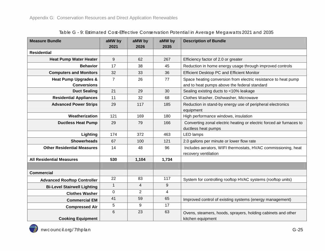
Appendix G: Conservation Resources and Direct Application Renewables
nwcouncil.org/7thplan G-25
Table G - 9: Estimated Cost-Effective Conservation Potential in Average Megawatts 2021 and 2035
Measure Bundle aMW by 2021
aMW by 2026
aMW by 2035
Description of Bundle
Residential Heat Pump Water Heater 9 62 267 Efficiency factor of 2.0 or greater
Behavior 17 38 45 Reduction in home energy usage through improved controls Computers and Monitors 32 33 36 Efficient Desktop PC and Efficient Monitor
Heat Pump Upgrades & Conversions
7 26 77 Space heating conversion from electric resistance to heat pump and to heat pumps above the federal standard
Duct Sealing 21 29 30 Sealing existing ducts to <10% leakage Residential Appliances 11 32 68 Clothes Washer, Dishwasher, Microwave Advanced Power Strips 29 117 185 Reduction in stand-by energy use of peripheral electronics
equipment Weatherization 121 169 180 High performance windows, insulation
Ductless Heat Pump 29 79 166 Converting zonal electric heating or electric forced air furnaces to ductless heat pumps
Lighting 174 372 463 LED lamps Showerheads 67 100 121 2.0 gallons per minute or lower flow rate
Other Residential Measures 14 48 96 Includes aerators, WIFI thermostats, HVAC commissioning, heat recovery ventilation
All Residential Measures 530 1,104 1,734 Commercial
Advanced Rooftop Controller 22 83 117 System for controlling rooftop HVAC systems (rooftop units)
Bi-Level Stairwell Lighting 1 4 9
Clothes Washer 0 2 4
Commercial EM 41 59 65 Improved control of existing systems (energy management)
Compressed Air 5 9 17
Cooking Equipment 6 23 63 Ovens, steamers, hoods, sprayers, holding cabinets and other
kitchen equipment

Appendix G: Conservation Resources and Direct Application Renewables
nwcouncil.org/7thplan G-26
Measure Bundle aMW by 2021
aMW by 2026
aMW by 2035
Description of Bundle
Embedded Data Centers 55 230 261 Direct Control Ventilation
Parking Garage 8 12 13
Direct Control Ventilation Restaurant Hood
6 8 8
Demand Control Ventilation 12 17 18
Desktop 13 28 56 ENERGY STAR desktop computers
DHP 12 43 60 Ductless heat pumps in commercial applications
ECM-VAV 4 12 30 Efficient motors in VAV applications
Economizer 18 26 26 Rooftop economizer improvements
Exterior Building Lighting 59 126 142
Grocery Refrigeration Bundle 37 52 57 Grocery store refrigeration measures
Laptop 0 1 4 ENERGY STAR laptop computers Light Emitting Capacitor
Exit Sign 4 9 19
Lighting Controls Interior 2 6 13 Interior lighting controls
Low Power LF Lamps 14 39 39
LPD Package 123 234 428 Interior lighting measures based on lighting power density
reduction Monitor 6 12 24
Motors Rewind 2 4 5
Municipal Sewage Treatment 14 32 35 Measures for municipal sewage treatment facilities
Municipal Water Supply 5 11 12
Parking lot Lighting 6 8 8
Premium Fume Hood 0 1 4
Pre-Rinse Spray Valve 1 1 1
Secondary Glazing Systems 1 5 10
Showerheads 3 4 4

Appendix G: Conservation Resources and Direct Application Renewables
nwcouncil.org/7thplan G-27
Measure Bundle aMW by 2021
aMW by 2026
aMW by 2035
Description of Bundle
Smart Plug Power Strips 30 42 47
Street and Roadway Lighting 30 57 61
VRF 5 25 78 Variable refrigerant flow systems
Water Cooler Controls 2 10 12
WEPT 3 7 7 Web-enabled programmable thermostats
Water Heater Tanks 0 1 2 Efficient water heater tanks All Commercial Measures 554 1,242 1,761 Industrial
Compressed Air 12 16 18 Efficient equipment and system optimization across all industries Energy Project Management 37 79 87 Multiple-system energy management, tracking and reporting in
large facilities Fans 26 54 60 Efficient equipment and system optimization across all industries
Refrigeration in Food Processing
9 12 14 Refrigeration equipment and system optimization
Controlled Atmosphere and Refrigeration in Food Storage
43 61 67 Refrigeration equipment and controlled atmosphere system optimization
Clean Room HVAC Systems in Hi-Tech
8 13 15 Industry-Specific Processes: Clean rooms and production facilities
Integrated Plant Energy Management
23 42 77 Top tier whole plant optimization in large facilities
Lighting 32 41 45 Lamp, ballast, fixture and control improvements across all industries
Material Handling 12 27 30 Efficient equipment and system optimization across all industries
Arc Furnaces in Metals 0.1 0.1 0.2 Industry-Specific Process: Arc furnace
Motors 0.0 0.0 0.0 Efficient motor rewinds across all industries Pulp Screening and Effluent
Treatment in Paper 3 5 10 Industry-Specific Process: Pulp screening, effluent treatment
Plant Energy Management 27 38 41 Multiple-system O&M in large facilities
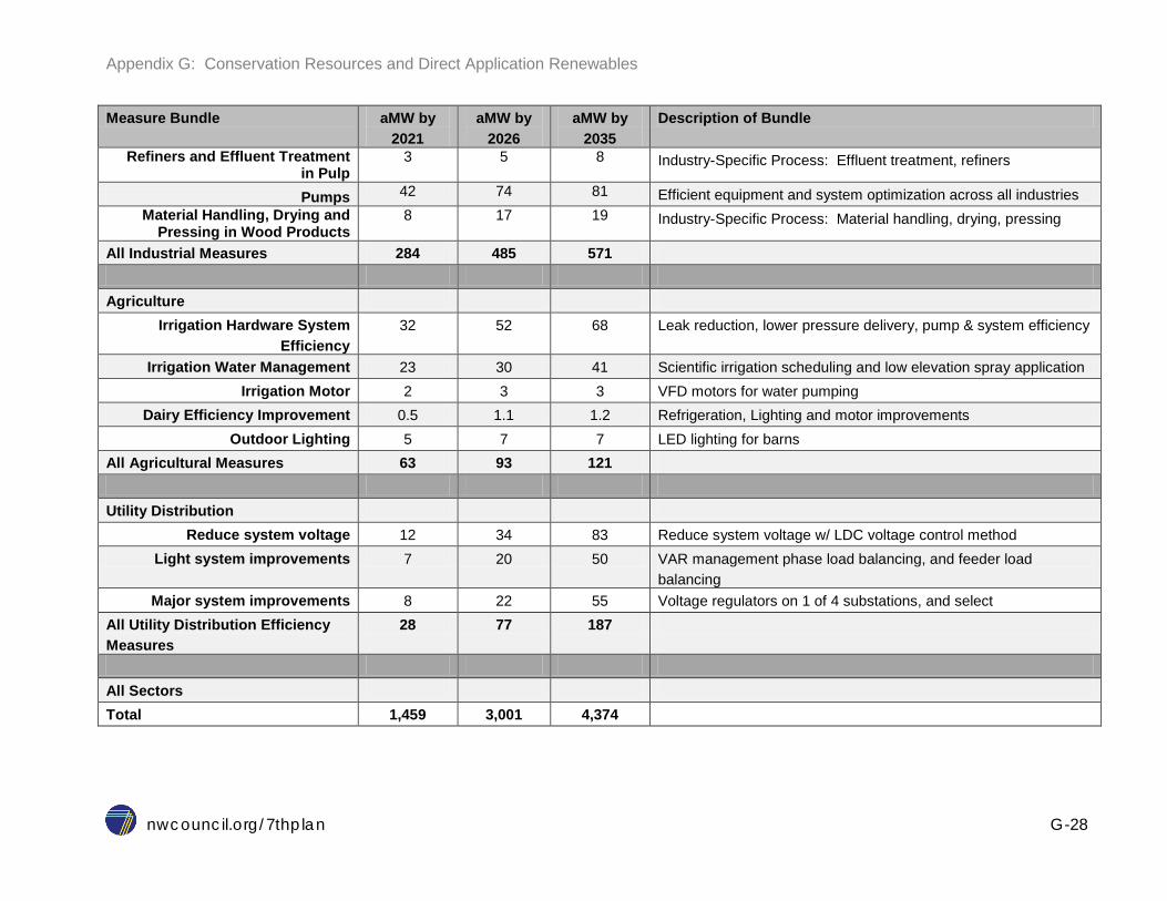
Appendix G: Conservation Resources and Direct Application Renewables
nwcouncil.org/7thplan G-28
Measure Bundle aMW by 2021
aMW by 2026
aMW by 2035
Description of Bundle
Refiners and Effluent Treatment in Pulp
3 5 8 Industry-Specific Process: Effluent treatment, refiners
Pumps 42 74 81 Efficient equipment and system optimization across all industries Material Handling, Drying and
Pressing in Wood Products 8 17 19 Industry-Specific Process: Material handling, drying, pressing
All Industrial Measures 284 485 571 Agriculture
Irrigation Hardware System Efficiency
32 52 68 Leak reduction, lower pressure delivery, pump & system efficiency
Irrigation Water Management 23 30 41 Scientific irrigation scheduling and low elevation spray application Irrigation Motor 2 3 3 VFD motors for water pumping
Dairy Efficiency Improvement 0.5 1.1 1.2 Refrigeration, Lighting and motor improvements Outdoor Lighting 5 7 7 LED lighting for barns
All Agricultural Measures 63 93 121 Utility Distribution
Reduce system voltage 12 34 83 Reduce system voltage w/ LDC voltage control method Light system improvements 7 20 50 VAR management phase load balancing, and feeder load
balancing Major system improvements 8 22 55 Voltage regulators on 1 of 4 substations, and select
All Utility Distribution Efficiency Measures
28 77 187
All Sectors Total 1,459 3,001 4,374
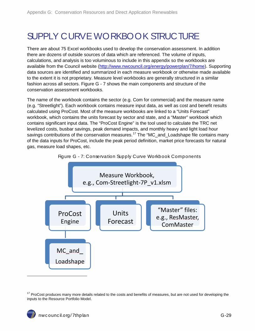
Appendix G: Conservation Resources and Direct Application Renewables
nwcouncil.org/7thplan G-29
SUPPLY CURVE WORKBOOK STRUCTURE There are about 75 Excel workbooks used to develop the conservation assessment. In addition there are dozens of outside sources of data which are referenced. The volume of inputs, calculations, and analysis is too voluminous to include in this appendix so the workbooks are available from the Council website (http://www.nwcouncil.org/energy/powerplan/7/home). Supporting data sources are identified and summarized in each measure workbook or otherwise made available to the extent it is not proprietary. Measure level workbooks are generally structured in a similar fashion across all sectors. Figure G - 7 shows the main components and structure of the conservation assessment workbooks.
The name of the workbook contains the sector (e.g. Com for commercial) and the measure name (e.g. “Streetlight”). Each workbook contains measure input data, as well as cost and benefit results calculated using ProCost. Most of the measure workbooks are linked to a “Units Forecast” workbook, which contains the units forecast by sector and state, and a “Master” workbook which contains significant input data. The “ProCost Engine” is the tool used to calculate the TRC net levelized costs, busbar savings, peak demand impacts, and monthly heavy and light load hour savings contributions of the conservation measures.17 The “MC_and_Loadshape file contains many of the data inputs for ProCost, include the peak period definition, market price forecasts for natural gas, measure load shapes, etc.
Figure G - 7: Conservation Supply Curve Workbook Components
17 ProCost produces many more details related to the costs and benefits of measures, but are not used for developing the inputs to the Resource Portfolio Model.
Measure Workbook, e.g., Com-Streetlight-7P_v1.xlsm
ProCost Engine
MC_and_ Loadshape
Units Forecast
“Master” files: e.g., ResMaster,
ComMaster

Appendix G: Conservation Resources and Direct Application Renewables
nwcouncil.org/7thplan G-30
The structure of each measure workbook is basically the same, as illustrated in Figure G - 8. The “7PSourceSummary” worksheet provides descriptive information about the measure and its sources. This is the best place to start when trying to understand the assumptions for a measure or measure bundle.
In addition, in each workbook, there are primarily two different types of worksheets: data input worksheets and supply curve results. The primary data input worksheet is called “Measure Input” or “M_Input_Out” or something similar. This sheet contains the specific measure cost, savings, life, and other parameters specific to each measure permutation. These are the data that get run through ProCost to determine, in part, the TRC net levelized cost of each measure. The other worksheets, typically to the right of the Measure Input sheet, are supporting data.
The supply curve results worksheets are shown to the left of the blue line in Figure G - 8. There could be three of these worksheets: new construction, natural replacement (NR), and retrofit applications. These sheets combine the measure data with information from the “Units Forecast” file to produce the technical achievable potential for the measure.
Figure G - 8: Conservation Supply Curve Workbook Structure
The layout of the “SC” worksheets is shown in Figure G - 9. This is where all of the measure-related data get pulled together to produce achievable technical potential estimates. It includes forecast data (e.g., housing units, commercial building floor area), application of ramp rates, applicability factors, and turnover rates. These data are used to produce the achievable number of units for a given measure, which are multiplied by measure unit savings. The potential estimates are then summed by levelized cost bin to produce the supply curve.
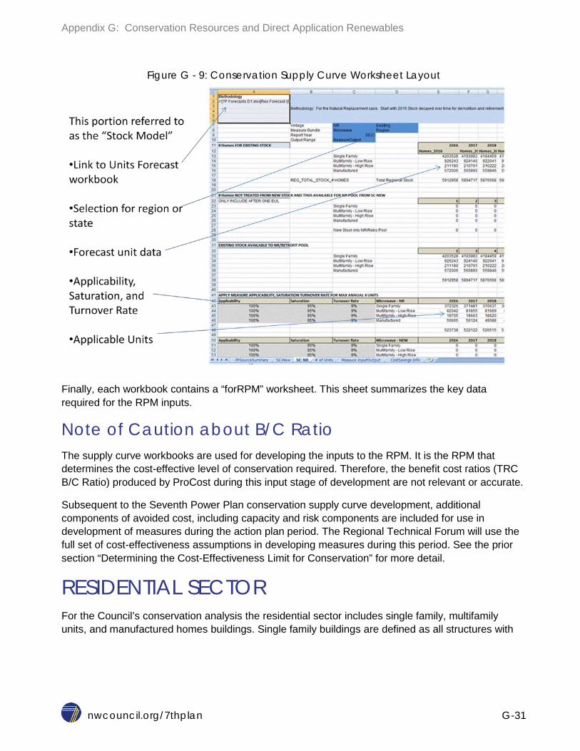
Appendix G: Conservation Resources and Direct Application Renewables
nwcouncil.org/7thplan G-31
Figure G - 9: Conservation Supply Curve Worksheet Layout
Finally, each workbook contains a “forRPM” worksheet. This sheet summarizes the key data required for the RPM inputs.
Note of Caution about B/C Ratio The supply curve workbooks are used for developing the inputs to the RPM. It is the RPM that determines the cost-effective level of conservation required. Therefore, the benefit cost ratios (TRC B/C Ratio) produced by ProCost during this input stage of development are not relevant or accurate.
Subsequent to the Seventh Power Plan conservation supply curve development, additional components of avoided cost, including capacity and risk components are included for use in development of measures during the action plan period. The Regional Technical Forum will use the full set of cost-effectiveness assumptions in developing measures during this period. See the prior section “Determining the Cost-Effectiveness Limit for Conservation” for more detail.
RESIDENTIAL SECTOR For the Council’s conservation analysis the residential sector includes single family, multifamily units, and manufactured homes buildings. Single family buildings are defined as all structures with

Appendix G: Conservation Resources and Direct Application Renewables
nwcouncil.org/7thplan G-32
four or fewer separate dwelling units, including both attached and detached homes. Multifamily structures include all housing with five our more dwelling units, up to four stories in height.18 Manufactured homes are dwellings regulated by the US Department of Housing and Urban Development (HUD) construction and safety standards (USC Title 42, Chapter 70). Modular homes, which are regulated by state codes, are considered single family dwellings.
One of primary inputs into the residential sector conservation assessment is the number of units that each conservation measure or measure bundle could be applied to in the region. Space conditioning savings are a function of both the characteristics of the structure and the climatic conditions where the home is located. Therefore, the Council’s assessment includes estimates of the number of new and existing dwelling units of each type (i.e., single family, multifamily, manufactured homes) in nine different climate zones. The Council defines climate zones by specific combinations of heating and cooling degree days. Table G - 10 shows the nine climate zones in the region.
Table G - 10: Regional Heating and Cooling Climate Zones
Climate Zone Heating Degree Days Cooling Degree Days Climate Zone: Heating 1 - Cooling 1 < 6,000 <300 Climate Zone: Heating 1 - Cooling 2 < 6,000 > 300 - 899 Climate Zone: Heating 1 - Cooling 3 < 6,000 > 900 Climate Zone: Heating 2 - Cooling 1 6,000 - 7,499 <300 Climate Zone: Heating 2 - Cooling 2 6,000 - 7,499 > 300 - 899 Climate Zone: Heating 2 - Cooling 3 6,000 - 7,499 > 900 Climate Zone: Heating 3 - Cooling 1 > 7,500 <300 Climate Zone: Heating 3 - Cooling 2 > 7,500 > 300 - 899 Climate Zone: Heating 3 - Cooling 3 > 7,500 > 900
Measure Bundles Nearly 60 residential-sector measures are analyzed in the Seventh Power Plan. These measure bundles do not and should not dictate the way measures are bundled for programmatic implementation. Many of the residential-sector measures are reviewed by the Regional Technical Forum (RTF) and incorporate those most recent data. However, in some cases, the final measures included in the Seventh Power Plan may be consolidated from the RTF measure list. For example, HVAC unit count information is of limited statistical significance between heating zones 2 and 3. As such, the savings for weatherization measures are estimated at the regional level, rather than individual climate zones, for each specific HVAC type. The measure bundles, each of which has an individual Excel workbook, are provided by end use in Table G - 11.
18 The conservation potential for water heating, lighting, appliances and consumer electronics in high rise multifamily dwellings (i.e., those covered by non-residential codes) are included in the residential sector. However, the savings from building shell and HVAC improvements in high rise multifamily buildings is not included in the Council’s assessment of regional conservation potential due to lack of data.

Appendix G: Conservation Resources and Direct Application Renewables
nwcouncil.org/7thplan G-33
Table G - 11: Residential Measure Bundles by End Use
End Use Measure Bundle(s) Dryer Heat pump clothes dryer
Electronics
Monitor Desktop Laptop Advanced power strips
Food Preparation Microwave Electric oven
HVAC
Controls, Commissioning, & Sizing Duct Sealing Ductless heat pump DHP with ducted system Ground-source heat pump Heat recovery ventilation Weatherization Air-source heat pump conversion ASHP upgrades Variable-capacity heat pump WIFI enabled thermostats
Lighting LED lighting LED lighting - pre 2020 Linear fluorescent lamps
Refrigeration Refrigerator Freezer
Water Heating
Aerator Clothes Washer Dishwasher Wastewater heat recovery Heat pump water heater Showerheads Solar water heater
Whole Bldg/Meter Level Behavior Electric vehicle supply equipment
As noted above, there are additional conservation measures that were not included in the Seventh Power Plan due to limited data or resources. Some of these measures are: hot water pipe insulation, variable-speed drive pump for well water, brushless permanent magnet motor for HVAC systems, whole house attic fans, reflective roofs, thermostatic shower restriction valves, and low-U doors.
Appendix G: Conservation Resources and Direct Application Renewables
nwcouncil.org/7thplan G-34
Overview of Methods For the residential sector measures, the unit of measure is a function of the measure type. Most measures apply to a fraction of the building stock in a particular building type. For example, insulation measures are a function of the number of households with electric heat, refrigerator efficiency improvements are a function of the number of refrigerators that are replaced or purchase new each year, and the potential savings from heat pump water heaters are function of the number of single family homes with electric water heating.
For every measure or practice analyzed, there are five major methodological steps to go through. These steps establish number of units, baseline conditions, measure applicability, and measure achievability. For the residential-sector conservation measures, each of these is treated explicitly for each measure bundle.
Physical Units
The conservation supply curves are developed primarily by identifying savings and cost per unit and estimating the number of applicable and achievable units that the measure can be deployed on. In the residential sector analysis, the applicable unit estimates for space conditioning, water heating, lighting, and appliances are based on the number of existing housing units and forecast of future housing growth from the Council’s Demand Forecasting Model. The housing units from the forecasting model were allocated to climate zones based on the population weighted average heating and cooling degrees for each county in the region. The housing unit data by state are contained in the Excel workbook entitled “7P Forecast.xls.” The estimates of physical units available include the number of units available annually. For example, for new buildings, the estimate of available new building stock is taken from the Council’s baseline forecast for annual additions by building type. Similarly for equipment replacement measures the annual stock available is taken from estimates of the turnover rate of the equipment in question. For retrofit measures, the annual stock availability is a fraction of the estimated stock remaining at the end of the forecast period. Most of the unit saturations are from the Residential Building Stock Assessment (RBSA), which provided a detailed analysis of homes across the region. The breakdown of measures by climate zone and building type is available in a workbook entitled “RBSA Saturations.xls”. These are incorporated into the individual supply curve workbooks as applicable. In addition, much of these data are also in the “Res_Master.xls” workbook.
Baseline Characteristics
Baseline conditions are estimated from current conditions for existing buildings and systems. Estimates of current conditions and characteristics of the building stock come from several sources. Key among these are the market research projects of the Northwest Energy Efficiency Alliance (NEEA), selected studies from utilities, Energy Trust of Oregon, and other sources.
For new buildings and new and replacement equipment, baseline conditions are estimated from a combination of surveys of new buildings, state and local building energy codes, and federal and state appliance efficiency standards. The most recent survey data for new buildings is from the NEEA New Single Family and New Multifamily Buildings Characteristics studies completed in 2007 which looked at buildings built in the 2003-2004. For existing buildings, the Residential Building
Appendix G: Conservation Resources and Direct Application Renewables
nwcouncil.org/7thplan G-35
Stock Assessment (RBSA), completed in 2012, is the source for saturations of most equipment and appliances.
Baseline characteristics for major appliances (washers, dishwashers, refrigerators, and freezers) are generally the national sales weighted average efficiency levels, or based on equipment appliance database from the California Energy Commission. Cost data for appliances was obtained from an analysis of the Oregon Residential Energy Tax Credit data and Internet searches. Heating, cooling, insulation, and window cost were obtained from an analysis of program data from Puget Sound Energy and the Energy Trust of Oregon. The assumptions were often tied to those determined by the Regional Technical Forum (RTF) in its development of unit energy savings.
Measure Applicability
There are hundreds of applicability assumptions in the residential-sector conservation assessment. Applicability assumptions by measure appear in the Res_Master workbook. The baseline saturation is provided in tab “BASE”, the technical feasibility is provided in the tab “FEAS”. The final applicability (the product of FEAS * (1 - BASE)) is provided on tab “APPLIC”.
Measure Achievability
The measure achievability is provided in the Res_Master workbook, tab “ACHIEV”. The overall ramp rates are given on the top of the sheet, while the mapping to each measure index name is provided below.
Guide to the Residential Conservation Workbooks Table G - 12 provides a cross-walk between the measures included in the Council’s assessment of regional conservation potential in the residential sector and the name of the individual workbooks. The most recent versions of these workbooks are posted on the Council’s website and are available for downloading http://www.nwcouncil.org/energy/powerplan/7/technical.

Appendix G: Conservation Resources and Direct Application Renewables
nwcouncil.org/7thplan G-36
Table G - 12: Residential Sector Supply Curve Input Workbooks
File Name File Scope Res_Master.xlsx Master workbook for residential conservation
modeling Res-Lighting-7P_v4.xlsx Lighting, above EISA 2020 requirements Res-Lighting_PPA-7P_v5.xlsx Short-term lighting below EISA 2020 requirements Res-LFLighting-7P_v1.xslx Linear fluorescent lighting in residential
applications Res-Dishwasher-7P_v4.xlsx Efficient Dishwasher Res-ClothesWasher-7P_v4.xlsx Efficient Clothes Washer Res-GFX-7P_v3.xlsx Gravity film heat exchanger Res-Showerhead-7P_v5.xlsx Low-flow showerheads Res-HPWH-7P_v4.xlsx Heat pump water heaters Res-EVCharger-7P_v2.xlsx Tier 2 electric vehicle supply equipment Res-ClothesDryer-7P_v2.xlsx Heat pump clothes dryer Res-RefrigFreezer-7P_v4.xlsm Efficient refrigerators and freezers Res-SWH-7P_v1.xlsx Solar water heater Res-Oven-7P_v3.xlsx Efficient ovens Res-Microwave-7P_v3.xlsx Efficient microwaves Res-Computers-7P_v4.xlsx Efficient desktop and laptop computers, and
monitors Res-SF_HP-7P_v5.xlsx Single-family heat pump (air-source and ductless)
conversions and upgrades Res-MH_HP-7P_v2.xlsx Manufactured homes heat pump (air-source and
ductless) conversions and upgrades Res-Duct_Seal-7P_v4.xlsx Duct sealing Res-WiFitstat-7P_v3.xlsx WiFi thermostat for heat pump controls Res-Aerator-7P_v5.xlsx Low-flow faucet aerator Res-COP-7P_v2.xlsx Behavior-program influenced reductions Res-HRV-7P_v1.xlsx Heat recovery ventilation in new construction Res-GSHP-7P_v2.xlsx Ground-source heat pump Res-FAF_to_DHP-7P_v2.xlsx Forced-air furnace to ductless heat pump
conversions Res-PowerStrips-7P_v6.xlsx Advanced power strips Res-CCS-7P_v4.xlsx Controls, commissioning, and sizing Res-SF_Wx-7P_v7.xlsx Single-family weatherization improvements Res-MF_Wx-7P_v6.xlsx Low-rise multi-family weatherization improvements Res-MH_Wx-7P_v4.xlsx Manufactured housing weatherization
improvements RBSA Saturations.xlsx Equipment and appliance saturations RTFStandardInformationWorkbook_v2_2.xls Costs and benefits information that is standard
across multiple measure assessments, developed by the RTF

Appendix G: Conservation Resources and Direct Application Renewables
nwcouncil.org/7thplan G-37
All of the individual measure files are linked to the “Res_Master.xls” file. This file contains the complete measure list, commercial building characteristics, baseline data, applicability factors, and ramp rates (achievability rates). The reference data in ResMaster are primarily in matrices by measure bundle and building type. The primary reference data in the ResMaster file are listed and described in Table G - 13.
Table G - 13: Reference Data in ResMaster Workbook
Sheet Name Contents Overview Overview of model structure MLIST Master list of measure bundles FILES List and links to measure-level files APPLIC Applicability factors for the measure. Calculated from data on FEAS and BASE. FEAS Technical feasibility for the measures. BASE Baseline penetration of the measure. Fraction of stock where the measure is already in place. STOCK Vintage cohort that the measure applies to TURN Turnover rate for stock to which measure applies, based on measure life ACHIEV Achievable rate of acquisition for measure bundles by year SATS Measure saturations by building type
COMMERCIAL SECTOR For the Council’s conservation analysis in the commercial sector, the majority of the conservation measures are derived based on savings per square foot of floor area by a specific building type. In a few other cases, a commercial conservation measure may be based on population (savings per person) or a direct estimate of unit count, such as the number of streetlights.
The commercial sector in the Pacific Northwest includes 3,350 million square feet in 2013, which are divided into 18 distinct building segments for analysis. Table G - 14 shows these segments and their associated floor area. Note that the office, retail, and food sales were further divided into categories by building size. In addition, over 900 million square feet of new floor space are expected to be added by 2035 based on the Council’s medium forecast.

Appendix G: Conservation Resources and Direct Application Renewables
nwcouncil.org/7thplan G-38
Table G - 14: Commercial Building Types
Primary Activity 7P Building Type Name Used in
Models Gross Floor Area
in Square Feet
Regional Floor Area (million sf)
Office Large Office Large Off >50,000 323 Office Medium Office Medium Off 5,000 to 50,000 316 Office Small Office Small Off <5,000 95 Retail Extra Large Retail Xlarge Ret >100,000 134 Retail Large Retail Large Ret 50,000 - 100,000 32 Retail Medium Retail Medium Ret 5000 - 50,000 346 Retail Small Retail Small Ret <5000 59 School School K-12 School K-12 Any 245 School University University Any 124 Warehouse Warehouse Warehouse Any 442 Retail Food Sales Supermarket Supermarket > 5000 65 Retail Food Sales MiniMart MiniMart < 5000 12 Restaurant Restaurant Restaurant Any 53 Lodging Lodging Lodging Any 171 Health Care Hospital Hospital Any 104 Health Care Residential Care Residential Care Any 125 Assembly Assembly Assembly Any 369 Other Other Other Any 333
Measure Bundles Nearly 40 individual commercial-sector measure bundles are analyzed in the Seventh Power Plan. These measures were bundled for analytical convenience and should not dictate the way measures are bundled for programmatic implementation. Table G - 15 shows these commercial sector measure bundles with their associated end-uses.
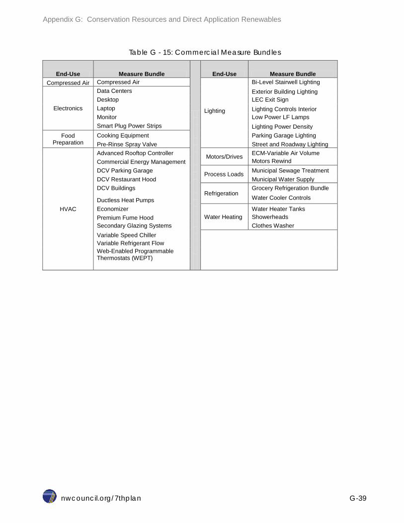
Appendix G: Conservation Resources and Direct Application Renewables
nwcouncil.org/7thplan G-39
Table G - 15: Commercial Measure Bundles
End-Use Measure Bundle
End-Use Measure Bundle Compressed Air Compressed Air
Lighting
Bi-Level Stairwell Lighting
Electronics
Data Centers Exterior Building Lighting Desktop LEC Exit Sign Laptop Lighting Controls Interior Monitor Low Power LF Lamps Smart Plug Power Strips Lighting Power Density
Food Preparation
Cooking Equipment Parking Garage Lighting Pre-Rinse Spray Valve Street and Roadway Lighting
HVAC
Advanced Rooftop Controller Motors/Drives ECM-Variable Air Volume Commercial Energy Management Motors Rewind DCV Parking Garage Process Loads Municipal Sewage Treatment DCV Restaurant Hood Municipal Water Supply DCV Buildings
Refrigeration
Grocery Refrigeration Bundle
Ductless Heat Pumps Water Cooler Controls
Economizer Water Heating
Water Heater Tanks Premium Fume Hood Showerheads Secondary Glazing Systems Clothes Washer Variable Speed Chiller
Variable Refrigerant Flow Web-Enabled Programmable Thermostats (WEPT)

Appendix G: Conservation Resources and Direct Application Renewables
nwcouncil.org/7thplan G-40
As noted in Chapter 12, there are additional conservation measures that were considered but not included in the Seventh Power Plan due to limited data or resources. There are undoubtedly cost-effective savings available from some of these measures and they should not be excluded from program consideration in plan implementation. These measures include:
AC Heat Recovery for Water Heating (& Reverse Cycle Chillers) Appliances - Freezers, Refrigerators Chiller retrofits Circulation pump ECM and drive Drain water heat recovery Elevator efficiency Energy recovery ventilator Engine generator block heaters Evaporative cooling Heat pump conversion & upgrade Heat pump water heaters Integrated Building Design19 Low pressure distribution complex HVAC Packaged refrigeration equipment Perimeter daylighting controls (Advanced) Pool blankets Pool pumps Premium HVAC equipment Roof insulation Signage Top daylighting Ultra low energy building Variable speed chiller Weatherization - School
19 The Sixth Power Plan included a measure called “Integrated Building Design” where synergistic effects of multiple measures in new buildings were captured as cost and performance savings above the application of individual measures. While the synergistic impacts of integrated design measures was not explicitly included in the Seventh Power Plan analysis, most new-building savings above code are being captured through individual measures in new buildings.

Appendix G: Conservation Resources and Direct Application Renewables
nwcouncil.org/7thplan G-41
Overview of Methods For the commercial sector measures, the unit of measure is a function of the measure type. Most measures apply to a fraction of the building floor area in a particular building type. For some measures, especially HVAC-related measures, the space heating fuel type is important. Some measures, like lighting, apply across all building types while others such as pre-rinse spray valves apply only to facilities with commercial kitchens.
For every measure or practice analyzed, there are five major methodological steps to go through. These steps establish number of units, baseline conditions, measure applicability, and measure achievability.
Physical Units
The conservation supply curves are developed primarily by identifying savings and cost per unit and estimating the number of applicable and achievable units for which the measure can be deployed. In the commercial sector analysis, the applicable unit estimates are based on the existing building floor area by building type and forecast of future new building growth from the Council’s Demand Forecasting Model. The floor space unit data by state are contained in the Excel workbook entitled “7P Forecast.xls.” The estimates of physical units available include the number of units available annually.
For example, for new buildings, the estimate of available new building stock is taken from the Council’s baseline forecast for annual floor area additions by building type. Similarly for equipment replacement measures the annual stock available is taken from estimates of the turnover rate of the equipment in question. For retrofit measures, the annual stock availability is a fraction of the estimated stock remaining at the end of the forecast period. These are incorporated into the individual supply curve workbooks as applicable. In addition, much of these data are in the “Com_Master.xls” workbook.
For some measures, the applicable units are based on other metrics such population and forecasted population growth. Table G - 16 shows examples of measure bundles and their corresponding unit savings basis and associated growth forecast.
Table G - 16: Commercial Measure Unit Savings Basis
Measure Bundle Unit Savings Basis Growth Forecast
Compressed Air kWh savings per motor horsepower Building floor space
Computers, laptops, monitors, power strips, pre-rinse spray valves, cooking equipment, water coolers
Count of units Population forecast
Water and wastewater Million gallons per day flow Population forecast All other measures Floor area by building type Building floor space

Appendix G: Conservation Resources and Direct Application Renewables
nwcouncil.org/7thplan G-42
Baseline Characteristics
Baseline conditions are estimated from current conditions for existing buildings and systems. Estimates of current conditions and characteristics of the building stock come from several sources. Key sources include the market research projects of the Northwest Energy Efficiency Alliance (NEEA), selected studies from utilities, Energy Trust of Oregon, and other sources.
For new buildings, new and replacement equipment, baseline conditions are estimated from a combination of surveys of new buildings, state and local building energy codes and federal and state appliance efficiency standards. The most recent survey data used is from the NEEA New Buildings Characteristics study completed in 2008 which looked at buildings built in the 2002-2004. In addition, data for the post 2004 cohort sample of the 2014 CBSA were used in some cases to represent new stock characteristics. Codes and standards are continually being upgraded. The baseline assumptions used for codes and standards in the Seventh Power Plan are those that were adopted by the end of 2014.
Baseline lighting systems are estimated from a combination of sources. The 2014 CBSA provided the mix of lighting systems types in common use by building type. There are five indoor fixture application types modeled each with separate baseline lamps and lighting power densities. A similar set of baselines characteristics is used for exterior lighting also based on CBSA. CBSA provided estimates of lighting power density and lighting hours of operation all of which are key components of the lighting baselines. Most lighting conservation measures are new, remodel, or replace on burnout situations where current practice baselines are used. To establish current practice baselines, CBSA lighting characteristics were adjusted to reflect applicable federal lighting standards and applicable state codes. For example, federal standards now require minimum efficacies for most four foot fluorescent lamps effective in 2014 and with an increase in efficacy mandated by 2018. A ballast efficacy standard also took effect in 2014. These federal standards reduce the lighting power densities for fluorescent lighting systems found in the CBSA because as the lamps and ballast burn out, they must be replaced with new more efficient models.
Embedded data centers are a growing end use in the commercial sector. The CBSA collected characteristics of data centers embedded in commercial buildings which established the baseline saturation of data centers and the equipment in them. Energy use in data centers is primarily driven by the density and utilization of the servers, storage, and network equipment with relatively fast turnover rates. No mandatory standards require minimum efficiencies for new and replacement equipment in data centers. Thus baseline estimates of efficiency are based instead on market trends and analysis of ENERGY STAR and other data. Significant commercial building modeling work was conducted in preparation of the Sixth Power Plan. The results of this work were again used to help establish baselines for some HVAC related measures in the Seventh Power Plan. For measures where significant achievements were recorded since the Sixth Power Plan, adjustments were made to the baseline electricity use intensity values.
Measure Applicability
There are hundreds of applicability assumptions in the commercial sector conservation assessment. Applicability assumptions by measure appear in the Com_Master workbook. The baseline saturation is provided in tab “BASE”, the applicability factors “APPLIC” and final applicability (1-BASE)*APPLIC

Appendix G: Conservation Resources and Direct Application Renewables
nwcouncil.org/7thplan G-43
is provided on tab “APPLIC”. For some measures, applicability factors reside in the measure workbook.
Measure Achievability
The measure achievability is provided in the Com_Master workbook, tab “ACHIEV”. The overall ramp rates are given on the top of the sheet, while the mapping to each measure index name is provided below.
Guide to the Commercial Conservation Workbooks Table G - 17 provides a cross-walk between the measures included in the Council’s assessment of regional conservation potential in the commercial sector and the name of the individual workbooks. The most recent versions of these workbooks are posted on the Council’s website and are available for downloading. http://www.nwcouncil.org/energy/powerplan/7/technical

Appendix G: Conservation Resources and Direct Application Renewables
nwcouncil.org/7thplan G-44
Table G - 17: Commercial Sector Supply Curve Input Workbooks
File Name File Scope Com_Master_7P.xlsx Master workbook for commercial conservation modeling Com-Bi-Level Stairwell-7P_V4.xlsx Bi-level stairwell lighting
COM-CompressedAir-7P_V4.xlsm Compressed air demand reduction, VFD, controls, and equipment upgrades
COM-Computers-7P_V3.xlsx Efficient desktop and laptop computers, and monitors
COM-Cooking-7P_V5.xlsm Efficient commercial steamers, hot food holding cabinets, combination ovens, fryers, and convection ovens
Com-DataCenters-7P_V6.xlsx Embedded data center improvements Com-DCV-7P_V5.xlsm Demand control ventilation COM-DCV-Garage-7P_V3.xlsm Demand control ventilation in enclosed parking garages COM-DCV-KitchenVent-7P_V3.xlsm Demand control ventilation for commercial kitchens COM-DHP-7P_V2.xlsm Ductless heat pumps for small commercial buildings COM-ECM-VAV-7P_V4.xlsm Electrically commutated motors for VAV systems COM-Economizer-7P_v2.xlsm Economizer maintenance and repair improvements Com-EM-7P_V5.xlsm Energy management (controls optimization) Com-ExitSign-7P_V3.xlsx Light Emitting Capacitor (LEC) exit signs Com-ExteriorLighting-7P_V14.xlsx Exterior lighting COM-FumeHood-7P_V2.xlsm Laboratory fume hood controls Com-Grocery-7P_V7.xlsx Grocery refrigeration system improvements Com-HPLowPowerGSFL-7P_V8.xlsx High performance low power fluorescent lamp Com-InteriorLightingControls-7P_V10.xlsx
Interior lighting controls
Com-LightingInterior-7P_v40.xlsx Interior lighting power density improvements COM-MotorsRewind-7P_v3.xlsm Motor rewinds Com-ParkingGarageLighting-7P_v7.xlsx Efficient lighting for parking garages COM-PowerStrips-7P_V5.xlsm Advances power strips for offices COM-PreRinseSpray-7P_V3.xlsm Pre-rinse valves for commercial kitchens Com-RooftopController-7P_V6.xlsm Advanced rooftop controller (ARC) COM-Showerhead-7P_v5.xlsm Low flow showerheads in hotels, athletic facilities Com-Streetlight-7P_V9.xlsx LED streetlights COM-VRF-7P_V6.xlsm Variable refrigerant flow HVAC systems COM-Washer-7P_V1.xlsm Commercial clothes washers COM-Wastewater-7P_V6.xlsm Municipal wastewater treatment system improvements Com-WaterCooler-7P_V6.xlsx Upgrade to ENERGY STAR water coolers and controls COM-WaterSupply-7P_V6.xlsm Municipal water supply system improvements COM-WEPT-7P_V2.xlsm Web-enabled programmable thermostats COM-WHTanks-7p_v6.xlsm Efficiency upgrades for tank-style electric water heaters Com-WindowSGS-7P_V5.xlsx Secondary glazing window systems (interior retrofit) Int_Light_Comp-7P_v2.xlsx Data development common to all lighting measures PNLPricePerfLED.xlsx Forecast of price and performance of solid state lighting Standard Information Workbook_v2.2 RTF data source for inputs common to all measures

Appendix G: Conservation Resources and Direct Application Renewables
nwcouncil.org/7thplan G-45
All of the individual measure files are linked to the “Com_Master_7P.xls” file. This file contains the complete measure list, commercial building characteristics, baseline data, applicability factors, and ramp rates (achievability rates). The reference data in ComMaster are primarily in matrices by measure bundle and building type. The primary reference data in the ComMaster file are listed and described in Table G - 18.
Table G - 18: Reference Data in ComMaster Workbook
Sheet Name Contents Overview Overview of model structure MLIST Master list of measure bundles FILES List and links to measure-level files APPLIC Applicability factors for the measure. Fraction of stock for which the measure applies BASE Baseline penetration of the measure. Fraction of stock where the measure is already in place STOCK Vintage cohort that the measure applies to TURN Turnover rate for stock to which measure applies ACHIEV Achievable rate of acquisition for measure bundles by year CHAR Key characteristics for stock by vintage and building subtype. Used to develop applicability FLOOR Floor area by building segment labels Building type list
INDUSTRIAL SECTOR The Seventh Power Plan’s assessment of conservation potential in the industrial sector covers a broad range of measures in 19 industrial segments, but excludes the direct service industries.20 The industrial sector utilizes a top-down methodology for estimating the conservation potential, so the key driver is total load by segment. The industrial segments and their 2016 (start year) and 2035 loads (end year) are shown in Table G - 19.
20 Direct service industries (DSIs) are large industrial facilities historically served directly by the Bonneville Power Administration.

Appendix G: Conservation Resources and Direct Application Renewables
nwcouncil.org/7thplan G-46
Table G - 19: Industrial Loads in 2016 and 2035
Industrial Segment 2016 aMW 2035 aMW Mechanical Pulp 336 486 Kraft Pulp 210 296 Paper 403 601 Foundries 105 77 Frozen Food 151 142 Other Food 275 364 Wood - Lumber 102 71 Wood - Panel 136 82 Wood - Other 250 174 Sugar 48 67 Hi Tech - Chip Fab 115 114 Hi Tech - Silicon 32 40 Metal Fab 139 76 Transportation, Equip 123 194 Refinery 87 131 Cold Storage 87 129 Fruit Storage 190 386 Chemical 264 513 Misc Manf 460 539 Total 3,514 4,482
Measure Bundles The industrial sector has a wide range of segments, end-using equipment, and function. The energy conservation measures need to apply to the end-use loads and therefore there is significant diversity in the number and type of industrial conservation measures. The industrial measure bundles are shown in Table G - 20.
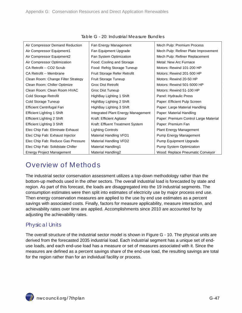
Appendix G: Conservation Resources and Direct Application Renewables
nwcouncil.org/7thplan G-47
Table G - 20: Industrial Measure Bundles
Air Compressor Demand Reduction Fan Energy Management Mech Pulp: Premium Process Air Compressor Equipment1 Fan Equipment Upgrade Mech Pulp: Refiner Plate Improvement Air Compressor Equipment2 Fan System Optimization Mech Pulp: Refiner Replacement Air Compressor Optimization Food: Cooling and Storage Metal: New Arc Furnace CA Retrofit -- CO2 Scrub Food: Refrig Storage Tuneup Motors: Rewind 101-200 HP CA Retrofit -- Membrane Fruit Storage Refer Retrofit Motors: Rewind 201-500 HP Clean Room: Change Filter Strategy Fruit Storage Tuneup Motors: Rewind 20-50 HP Clean Room: Chiller Optimize Groc Dist Retrofit Motors: Rewind 501-5000 HP Clean Room: Clean Room HVAC Groc Dist Tuneup Motors: Rewind 51-100 HP Cold Storage Retrofit HighBay Lighting 1 Shift Panel: Hydraulic Press Cold Storage Tuneup HighBay Lighting 2 Shift Paper: Efficient Pulp Screen Efficient Centrifugal Fan HighBay Lighting 3 Shift Paper: Large Material Handling Efficient Lighting 1 Shift Integrated Plant Energy Management Paper: Material Handling Efficient Lighting 2 Shift Kraft: Efficient Agitator Paper: Premium Control Large Material Efficient Lighting 3 Shift Kraft: Effluent Treatment System Paper: Premium Fan Elec Chip Fab: Eliminate Exhaust Lighting Controls Plant Energy Management Elec Chip Fab: Exhaust Injector Material Handling VFD1 Pump Energy Management Elec Chip Fab: Reduce Gas Pressure Material Handling VFD2 Pump Equipment Upgrade Elec Chip Fab: Solidstate Chiller Material Handling1 Pump System Optimization Energy Project Management Material Handling2 Wood: Replace Pneumatic Conveyor
Overview of Methods The industrial sector conservation assessment utilizes a top-down methodology rather than the bottom-up methods used in the other sectors. The overall industrial load is forecasted by state and region. As part of this forecast, the loads are disaggregated into the 19 industrial segments. The consumption estimates were then split into estimates of electricity use by major process end use. Then energy conservation measures are applied to the use by end use estimates as a percent savings with associated costs. Finally, factors for measure applicability, measure interaction, and achievability rates over time are applied. Accomplishments since 2010 are accounted for by adjusting the achievability rates.
Physical Units
The overall structure of the industrial sector model is shown in Figure G - 10. The physical units are derived from the forecasted 2035 industrial load. Each industrial segment has a unique set of end-use loads, and each end-use load has a measure or set of measures associated with it. Since the measures are defined as a percent savings share of the end-use load, the resulting savings are total for the region rather than for an individual facility or process.

Appendix G: Conservation Resources and Direct Application Renewables
nwcouncil.org/7thplan G-48
Figure G - 10: Industrial Model Structure
Baseline Characteristics
The baseline characteristics of the industrial sector are defined by the electricity end-uses in each of the segments. The original research and model development for the industrial sector was conducted prior to the development of the Sixth Power Plan. For the Seventh Power Plan, the same model, methodology and measure list were used. However, significant updates were made to the baseline conditions.
One of the primary baseline components is the industrial load by segment (shown previously in Table G - 19). These baselines loads are based on the regional end-use load forecast for the industrial sector (see Chapter 7 and Appendix E). Loads for each segment were developed using a variety of sources including the Industrial Facility Site Assessment (IFSA).
A second major baseline component is the share of consumption by end-use. Estimated end-use shares from the Sixth Plan were reviewed and revised using new data sources including the IFSA and the Energy Information Agency’s 2010 Manufacturing Energy Consumption Survey.
Finally, measure baseline saturation updates were made by reviewing the conservation measures completed since the Sixth Power Plan. Data were provided by the Six Going on Seven project sponsored by BPA, which included data from 2010-2013. Savings data were projected for 2014 and 2015. These achieved savings were used to update the baseline saturation of measures.
Industrial Load (2035)
Segment Load (e.g., Paper)
Segment End-Use 1 (e.g.,Material
Handling)
Segment End-Use 2 (e.g., Pumps)
Measure 1 - Pump energy
management
Measure 2 - Pump equipment
upgrade
Measure 3 - Pump System
Optimization
Segment End-Use 3 (e.g., Lighting)
Segment Load (e.g., Cold Storage) Etc...

Appendix G: Conservation Resources and Direct Application Renewables
nwcouncil.org/7thplan G-49
Measure Applicability
Each of the 60 or so industrial measures has a physical applicability number associated with it, along with a “fraction incomplete” factor. The combination of these makes up the measure applicability.
Measure Achievability
The industrial measure technical achievability is largely 85 percent, similar to the other sectors. However, the industrial sector has a few measures that have less than 85 percent achievability due to limiting factors within a given industry or measure group, including the electronic chip fabrication (25%), pulp and paper (50%), and energy management (50%-75%). New ramp rates were applied to the measures for the Seventh Power Plan. Since most of these measures were new in the Sixth Power Plan, the pace of achievement since 2010 played a significant role in selection and application of ramp rates. The industrial measures are all considered retrofit.
Guide to the Industrial Sector Workbooks and Data Table G - 21 provides of the individual workbooks utilized in the industrial sector assessment. The most recent versions of these workbooks are posted on the Council’s website and are available for downloading. http://www.nwcouncil.org/energy/powerplan/7/technical
Table G - 21: Industrial Sector Supply Curve Input Workbooks
Item Description
Measure Analysis Tool
Industrial_tool_7thPlan v09.xlsm
Excel workbook containing the major elements of the industrial sector characterization, the estimates of end use splits and the details on the energy conservation measures
NPCC Supply Curve
IND-All-7P-v5.xlsm
Excel workbook which translates the costs and savings from the Measure Analysis Tool into supply curve data for the Regional Portfolio Model. Uses ProCost to develop TRC Net levelized costs.
Achievements and Applicability Adjustments
Achievements and Applicability v07.xlsm
This workbook contains the detailed data and mapping for the measures and measure saturation. The IFSA and the Six Gong on Seven data were utilized for updating measure baselines.
Systems Whole Plant Optimization Overview
Description of the system optimization and whole plant measure bundles, the input assumptions, and supporting sources. This document was created for the Sixth Power Plan, but the Seventh Plan utilizes the same measures.
Industrial Lighting Analysis
IND-Lighting-7P_V2.xlsx
This workbook contains a separate industrial lighting analysis based on data from the Industrial Facilities Site Assessment.

Appendix G: Conservation Resources and Direct Application Renewables
nwcouncil.org/7thplan G-50
AGRICULTURAL SECTOR The Seventh Power Plan’s assessment of conservation potential in the agriculture sector covers irrigation hardware system efficiency improvements, irrigation water management (scientific irrigation scheduling [SIS] and low-energy spray application [LESA]), and dairy farm milk processing. Consistent with the conservation assessments in prior plan’s, the largest potential savings in the agriculture sector are available through irrigation hardware system efficiency improvements, including reducing system operating pressures, reducing system leaks, and improving pump efficiency. The next largest savings in this sector come from improved water management practices followed by efficient barn lighting and dairy milk processing savings. This is the first Council plan to estimate savings from LESA and efficient barn lighting.
Measure Bundles Seven measure bundles are considered in the Seventh Power Plan, five of which are irrigation measures. The five irrigation bundles are:
1. Generic irrigation hardware system efficiency improvements and three “operation and maintenance” (e.g., gasket and nozzle replacement) measures,
2. Irrigation water management practices were considered as a bundled measure consisting of moisture monitoring hardware and software,
3. Converting high/medium pressure center pivot systems to low-pressure systems, 4. Low-elevation spray application, using ultra-low pressure (<10psi) center pivot
systems, 5. Efficient green motor rewind practices for irrigation motors.
The remaining two measure bundles include improving the energy efficiency of dairy milking barns and milk processing and converting barn area lighting to high-efficiency LEDs.
As noted above, the Seventh Power Plan does not include all potential measures. Some missing measures include: high-volume low-speed fans, variable speed drives for well pumps, and low-energy livestock waterer. Also, efficiency improvements for indoor agriculture (including greenhouses) were not explicitly analyzed.
Overview of Methods Many of the assumptions for agriculture measures are based on Sixth Power Plan assumptions. Exceptions are irrigation hardware efficiency, barn area lighting, and green motor rewinds, which have incorporated recent RTF analysis. The Seventh Power Plan has updated irrigated acreage assumptions from the 2013 Farm and Ranch Irrigation Survey.
Irrigation water management savings (SIS) were estimated using a spreadsheet developed by the Columbia Basin Ground Water Management Association (GAMA). This spreadsheet was modified to reflect the average water savings achieved in Bonneville’s 2005 study of irrigation water management practices. This evaluation documented the average water savings from scientific irrigation water management as well as the cost of carrying out improved practices. This approach is

Appendix G: Conservation Resources and Direct Application Renewables
nwcouncil.org/7thplan G-51
equivalent to that used in the Sixth Power Plan. Research to be completed in 2016 will better inform available acreage for SIS and baseline practices.
Dairy efficiency improvements were based on detailed audits and retrofits of 30 dairies in New York carried out by the New York State Energy Research and Development Administration (NYSERDA). This approach is equivalent to that used in the Sixth Power Plan. However, baseline saturations were adjusted upwards to account for many of the measures becoming standard practice.
Physical Units
The conservation supply curves are developed primarily by identifying savings and cost per unit and estimating the number of applicable and achievable units that the measure can be deployed on. In the irrigation sector analysis, the applicable unit estimates for irrigated acreage, system types and annual water application were drawn from the 2013 USDA Farm and Ranch Irrigation Survey (FRIS). GAMA provided data on the acreage and crop types present in Columbia Basin Project. The estimate of current diary production in the region also comes from the USDA and the US Department of Commerce. Staff developed a forecast of future milk production growth in the region using historical trends.
Baseline Characteristics
Baseline conditions for irrigation hardware system efficiency improvements were estimated from the USDA Farm and Ranch Irrigation Survey and discussions with Bonneville and utility staff with in-depth experience working with farmers on these systems. Baseline characteristics (i.e., the average amount of water applied by crop type and acreage) for irrigation water management in the Columbia Basin Project was provided by GAMA. Dairy efficiency in the region was assumed to parallel that found by NYSERDA.
Measure Applicability and Measure Achievability
No quantitative study has been conducted in the region to determine the current saturation and remaining opportunities for improvement in either irrigation system hardware or on diaries. Therefore, judgment, based on discussions with Bonneville and utility program staff served as the basis estimating the remaining number of systems and diaries in the region that could carry out cost-effective energy efficiency improvements. Where quantitative data was available (e.g. the acreage irrigated with high pressure systems), these data were used to size the remaining opportunities for savings.
Guide to the Agriculture Conservation Workbooks The eight workbooks containing the Agriculture Sector conservation resource assessment are downloadable from the web http://www.nwcouncil.org/energy/powerplan/7/technical. These are provided in Table G - 22.
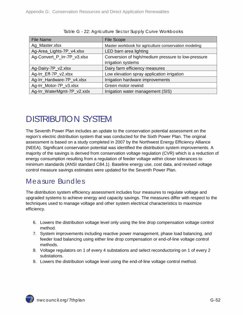
Appendix G: Conservation Resources and Direct Application Renewables
nwcouncil.org/7thplan G-52
Table G - 22: Agriculture Sector Supply Curve Workbooks
File Name File Scope Ag_Master.xlsx Master workbook for agriculture conservation modeling Ag-Area_Lights-7P_v4.xlsx LED barn area lighting Ag-Convert_P_Irr-7P_v3.xlsx Conversion of high/medium pressure to low-pressure
irrigation systems Ag-Dairy-7P_v2.xlsx Dairy farm efficiency measures Ag-Irr_Eff-7P_v2.xlsx Low elevation spray application irrigation Ag-Irr_Hardware-7P_v4.xlsx Irrigation hardware improvements Ag-Irr_Motor-7P_v3.xlsx Green motor rewind Ag-Irr_WaterMgmt-7P_v2.xslx Irrigation water management (SIS)
DISTRIBUTION SYSTEM The Seventh Power Plan includes an update to the conservation potential assessment on the region’s electric distribution system that was conducted for the Sixth Power Plan. The original assessment is based on a study completed in 2007 by the Northwest Energy Efficiency Alliance (NEEA). Significant conservation potential was identified the distribution system improvements. A majority of the savings is derived from conservation voltage regulation (CVR) which is a reduction of energy consumption resulting from a regulation of feeder voltage within closer tolerances to minimum standards (ANSI standard C84.1). Baseline energy use, cost data, and revised voltage control measure savings estimates were updated for the Seventh Power Plan.
Measure Bundles The distribution system efficiency assessment includes four measures to regulate voltage and upgraded systems to achieve energy and capacity savings. The measures differ with respect to the techniques used to manage voltage and other system electrical characteristics to maximize efficiency.
6. Lowers the distribution voltage level only using the line drop compensation voltage control
method. 7. System improvements including reactive power management, phase load balancing, and
feeder load balancing using either line drop compensation or end-of-line voltage control methods.
8. Voltage regulators on 1 of every 4 substations and select reconductoring on 1 of every 2 substations.
9. Lowers the distribution voltage level using the end-of-line voltage control method.

Appendix G: Conservation Resources and Direct Application Renewables
nwcouncil.org/7thplan G-53
Overview of Methods The distribution system conservation assessment uses savings estimates from measured data on actual projects conducted on utility feeders over the course of one year, or more from the 2007 study and subsequent data from a few more recent projects. Savings are a function of the reduction in voltage, the end-use equipment at customers’ sites including the mix of resistive and conductive loads, and electrical characteristics of the distribution system configuration. Savings estimates vary by utility for the largest utilities. For smaller utilities, average system characteristics from the measured data set were used to represent electrical and load conditions in smaller utilities. Savings also differ across residential, commercial and industrial feeders. Savings on residential feeders are highest. Costs and savings for four major measures were identified and applied to a descriptive data set of the region’s distribution system. The dataset contains system loads by customer class, substation counts, feeder counts, customer counts and climate zones for 137 regional utilities. Savings accomplished since the Sixth Power Plan were accounted for.
Physical Units
The distribution efficiency savings, especially conservation voltage regulation, come from adjusting the feeder voltage which results in a small percentage of the overall kWh consumption. Therefore, the primary units are the total electricity sales by utility, along with the number and type of substations for the utility.
Baseline Characteristics
Baseline updates include the savings accomplishments, updated regional energy use (2012, by utility), and updated knowledge about utility-specific savings inputs.
Measure Applicability
Measure applicability is estimated for residential, commercial and industrial feeders by measure. Applicability is highest for residential feeders (80 – 85 percent) and lowest for industrial feeders (10 – 15 percent). Two key factors which drive the savings are conservation voltage regulation factor and the percent change in voltage achievable. These are taken from the 2007 NEEA study or subsequent utility-specific updates. These input assumptions are worksheet ‘RegionWideSubstations’.
Measure Achievability
The Council generated a very slow ramp rate for achievability based on regional experience with the measures to date and advice from its Conservation Resources Advisory Committee. The ramp rate is unique to the distribution efficiency measure set. Sheet ‘ACHIEV’ contains the details.
Guide to the Distribution Efficiency Workbooks The distribution efficiency data and calculations are contained in a single workbook (see Table G - 23), available on the web http://www.nwcouncil.org/energy/powerplan/7/technical. One of the key worksheets in this file is called “RegonWideSubstations” that contains a listing of utilities and

Appendix G: Conservation Resources and Direct Application Renewables
nwcouncil.org/7thplan G-54
associated data for the DE measures. Selected other worksheets and their corresponding scopes are also listed in Table G - 23.
Table G - 23: Distribution System Supply Curve Workbook
File Name File Scope DE-Distribution-7P_V4.xlsx This file contains all data and calculates for the DE
assessment Worksheet Name Worksheet Scope
SC-Retro Contains the final DE supply curve 7PSourceSummary Descriptive information about the measures and assumptions Rollup Summary of the measure data RegionWideSubstations Detailed substation information by utility, applicability factors,
savings factors, calculations of savings potential by utility and measure and regional totals
Approach for 7th Plan Descriptive summary of the approach SixGoingOnSeven Measure achievement data since the Sixth Power Plan
DISTRIBUTED PHOTOVOLTAICS Distributed solar photovoltaics (distributed PV) are broadly considered “behind-the-meter” PV panels that are generally mounted on the rooftop of a house, commercial building, or other structure to provide on-site electricity. The primary use of this electricity is for the building with any excess generation sold back to the grid or stored in batteries.
Measure Bundles The Council’s analysis considered the potential from distributed PV for the residential and commercial sectors, considering installations on both the west and east side of the Cascade Mountains, to account for variant insolation levels. For analytic simplicity, Portland, Oregon was used as the proxy for the west-side installation, and Boise, Idaho was the proxy for the east-side installations. There were four measure bundles considered:
1. Residential west side 2. Residential east side 3. Commercial west side 4. Commercial east side

Appendix G: Conservation Resources and Direct Application Renewables
nwcouncil.org/7thplan G-55
Overview of Methods The Council estimated the potential for distributed PV based on roof area estimates taken from the recent Pacific Northwest residential and commercial stock assessments, accounting for shading factors and rooftop orientation. The solar calculator PVWatts®21 was used to set the expected annual capacity factor for both the east and west side of the Cascade Mountains. PVWatts also produces hourly generation shapes. Costs are based on 2014 program data from Energy Trust of Oregon, with assumptions of cost declines, resulting in a 2025 cost of about 66 percent of 2014 costs. As a final step, costs were adjusted between 2016 and 2021 to reflect the federal solar tax credit adopted in 2015. The overall approach to estimating the technical potential for distributed PV is provided in Figure G - 11, where the details are discussed below.
Figure G - 11: Approach to estimating PV technical potential
Physical Units
The distributed PV potential is estimated based on the total area of residential and commercial roofs.22 The Council estimates approximately 2.6 billion square feet of commercial roof area by 2035. For residential buildings, the total roof area is calculated from the assumed average single family home size (2,300 square feet), number of stories (1.4 per home), and total number of buildings (6.3 million in 2035), totaling approximately 10.4 billion square feet.
Not all the available roof area is usable for a PV array. Obstructions, shading, and orientation all limit where an array could be mounted. The Council used estimates of 25 percent of available roofs for residential and 60 percent for commercial can have a PV array.23 As such, the available roof area
21 http://rredc.nrel.gov/solar/calculators/pvwatts/version1/change.html 22 Industrial rooftops were not considered as part of the analysis. 23 DNV GL, A Review of Distributed Energy Resources for NYISO, 2014
• Number of rooftops
• Area per roof Total roof area
• Shading • Obstructions • Orientation
Roof area for PV
• Array power density (Watts per square foot) Watts
• Capacity factor for east and west Energy

Appendix G: Conservation Resources and Direct Application Renewables
nwcouncil.org/7thplan G-56
decreases to 2.4 billion square feet for residential and 1.6 billion square feet for commercial. These roofs are split approximately 34 percent on the east side and 66 percent on the west side.
Baseline Characteristics
To estimate the energy generated from the arrays, the Council assumed an array power density of 12.4 watts per square foot.23 This results in a total distributed PV nameplate capacity technical potential of about 50,000 megawatts (DC) in 2035. To estimate the energy produced, the Council used PVWatts which estimated the average capacity factor for distributed PV as 13 percent for the west side and 17 percent for the east side of the Cascades. The resulting total technical potential is about 5,500 average megawatts in 2035.
Measure Applicability and Achievability
Rooftop solar PV is an emerging technology. There are many barriers to complete adoption of what is technically achievable. The Council estimated the maximum achievable technical potential based on sensitivity analysis done by the National Renewable Energy Lab (NREL) as part of its SunShot Vision project, an assessment in which solar provides a significant share of electricity demand in the U.S. The NREL study analyzed many factors that will influence the pace of penetration of rooftop PV. These included PV prices, regional solar resources, local electricity rates, financing structures, net-metering policy, incentives, and other market characteristics. Figure G - 12 shows the ramp rates that the Council developed from the NREL study to estimate achievable fractions of technical potential by year. The figure shows the high and low range of achievability as well as the potential assumed to be adopted in the baseline demand forecast.

Appendix G: Conservation Resources and Direct Application Renewables
nwcouncil.org/7thplan G-57
Figure G - 12: Ramp Rates for Achievable Solar PV Potential
Measure Costs
The costs for distributed PV are based on Energy Trust of Oregon program data, for residential and commercial systems. PV has experience rapid decrease in costs in the past few years and these declines are projected to continue. The projected costs for distributed PV declines at the same rates as those used for utility-scale PV (see Chapter 13) and are based on a variety of secondary sources including cost trends from projects planned and constructed in the 2010-2016 period plus forecast estimates from several consulting groups and NREL. The total installation costs (all in 2012$) are summarized in Figure G - 13. The figure reflects the expected decrease in cost of distributed PV due to technical innovation and production volume as well as the federal tax credit currently available. Federal legislation extending the Solar Investment Tax Credit (ITC) was signed into law on December 18th, 2015. The bill extends the 30 percent Solar Investment Tax Credits for both residential and commercial projects through the end of 2019, and then drops the credit to 26 percent in 2020, and 22 percent in 2021 before dropping permanently to 10 percent for commercial projects and 0 percent for residential projects.
-
5,000
10,000
15,000
20,000
25,000
30,000
2016
2017
2018
2019
2020
2021
2022
2023
2024
2025
2026
2027
2028
2029
2030
2031
2032
2033
2034
2035
MW
Cap
acity
Ach
ieva
ble
Pote
ntia
l for
So
lar R
ooof
top
PV
SunShot High
SunShot
7P Baseline Medium
7P Baseline High

Appendix G: Conservation Resources and Direct Application Renewables
nwcouncil.org/7thplan G-58
Figure G - 13: Forecast of Distributed PV Costs
In addition to the installation costs, there is an inverter replacement cost and an annual O&M cleaning cost. Cost estimates for these factors are taken from the NREL studies. An estimate of system integration costs is also included. Bonneville integrations costs from its 2014 tariff were used to estimate integrations costs.
Daily and Seasonal Shape and Capacity Contribution
The solar calculator PVWatts® was used to estimate the hourly, daily and monthly energy, and summer and winter peak contribution of rooftop PV. Figure G - 13 shows Heavy Load Hour (HHL) and Light Load Hour (LLH) energy by month for typical residential applications in Boise and Portland. Daytime energy production is nearly three times higher in summer months than in winter months in both locations. Off hour production is very small relative to daytime heavy load hour production.
$-
$500
$1,000
$1,500
$2,000
$2,500
$3,000
$3,500
$4,000
$4,500
$5,000
Inst
alle
d Co
st p
er kW
DC
in 2
012$
Year
Residential
Commercial
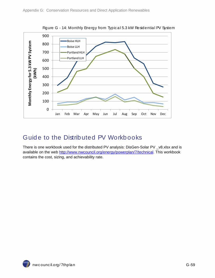
Appendix G: Conservation Resources and Direct Application Renewables
nwcouncil.org/7thplan G-59
Figure G - 14: Monthly Energy from Typical 5.3 kW Residential PV System
Guide to the Distributed PV Workbooks There is one workbook used for the distributed PV analysis: DisGen-Solar PV _v8.xlsx and is available on the web http://www.nwcouncil.org/energy/powerplan/7/technical. This workbook contains the cost, sizing, and achievability rate.
0
100
200
300
400
500
600
700
800
900
Jan Feb Mar Apr May Jun Jul Aug Sep Oct Nov Dec
Mon
thly
Ener
gy fo
r 5.3
kW P
V Sy
stem
(k
Wh)
Boise HLH
Boise LLH
Portland HLH
Portland LLH

Seventh Northwest Conservation and Electric Power Plan
nwcouncil.org/7thplan H-1
APPENDIX H: GENERATING RESOURCES – BACKGROUND INFORMATION
Contents Introduction ....................................................................................................................................... 3 General Methodology and Assumptions ............................................................................................ 3
Generating Resources Assessment Methodology .......................................................................... 4 Quantifying Environmental Effects ............................................................................................. 7
Resource Attributes ....................................................................................................................... 7 Generating Resource Reference Plants ............................................................................................ 9
Combined Cycle Combustion Turbine ............................................................................................ 9 Reciprocating Engine ................................................................................................................... 13 Simple Cycle - Aeroderivative Gas Turbine .................................................................................. 16 Simple Cycle - Frame Gas Turbine .............................................................................................. 19 Utility-Scale Solar Photovoltaic .................................................................................................... 22 Wind Power: Utility Scale, Onshore ............................................................................................. 25 Geothermal: Conventional ........................................................................................................... 29 Transmission ............................................................................................................................... 32 Long-term Resource: Utility-Scale Solar PV + Battery Energy Storage System ........................... 33 Regional Portfolio Model .............................................................................................................. 36

Appendix H: Generating Resources
nwcouncil.org/7thplan H-2
List of Figures and Tables
Table H - 1: Classification of Generating Resources* ....................................................................... 4 Figure H - 1: Generating Resources Assessment ............................................................................. 5 Figure H - 2: Capital Cost Estimate for Aeroderivative Gas Turbines ................................................ 6 Table H - 2: Financial Assumptions for Project Sponsors .................................................................. 7 Table H - 3: CCCT Reference Plants.............................................................................................. 11 Table H - 4: CCCT Cost Summary ................................................................................................. 12 Table H - 5: Reciprocating Engines Reference Plants .................................................................... 14 Table H - 6: Reciprocating Engine Cost Summary .......................................................................... 15 Table H - 7: Aeroderivative Gas Turbine Reference Plants ............................................................ 17 Table H - 8: Aeroderivative Gas Turbine Cost Summary ................................................................ 18 Table H - 9: Frame Gas Turbine Reference Plants ......................................................................... 20 Table H - 10: Frame Gas Turbine Cost Summary ........................................................................... 21 Table H - 11: Solar PV Reference Plants ....................................................................................... 23 Table H - 12: Solar PV Cost Summary ........................................................................................... 24 Figure H – 3: Simulated Monthly Solar Plant Output for Southern Idaho ......................................... 25 Table H - 13: Wind Power Reference Plants .................................................................................. 27 Table H - 14: Wind Power Cost Summary ...................................................................................... 28 Table H - 15: Conventional Geothermal Reference Plants ............................................................. 31 Table H - 16: Conventional Geothermal Cost Summary ................................................................. 31 Figure H - 4: Modeled Example of Solar + Battery System ............................................................. 34 Table H - 17: Utility Scale Solar PV Plant ........................................................................................ 35 Table H - 18: Lithium Ion Battery Storage System ........................................................................... 35 Table H - 19: Cost estimate for combined Utility Scale Solar PV + Lithium Ion Battery Storage System ............................................................................................................................................ 36 Table H - 20: Generating Resources and the Regional Portfolio Model ........................................... 37

Appendix H: Generating Resources
nwcouncil.org/7thplan H-3
INTRODUCTION This appendix describes the development of the planning assumptions for new generating resource and energy storage alternatives for use in the Seventh Power Plan.
GENERAL METHODOLOGY AND ASSUMPTIONS As described in Chapter 13, the Council prioritized and categorized generating resources based on a resource’s commercial availability, constructability, and developable potential in the Pacific Northwest during the 20-year power planning period. The three classifications used to analyze resources were: Primary: Significant resources that are deemed proven, commercially available, and
deployable on a large scale in the Pacific Northwest at the start of the power planning period. These resources have the potential to play a major role in the future regional power system. Primary resources receive an in-depth, quantitative assessment to support system integration and risk analysis modeling. Primary resources are modeled in the Regional Portfolio Model (RPM).
Secondary: Commercially available resources with limited, or small-scale, developmental potential in the Pacific Northwest. While secondary resources are currently in-service or available for development in the region, they generally have limited potential in terms of resource availability or typical plant size. Secondary resources receive at least a qualitative assessment to estimate status and potential and sometimes a quantitative assessment to estimate cost. While secondary resources are not explicitly modeled in the RPM, they are still considered viable resource options for future power planning needs.
Long-term: Emerging resources and technologies that have a long-term potential in the Pacific Northwest but are not commercially available or deployable on a large scale at the beginning of the power planning period. Long-term resources receive a qualitative assessment and if available, quantification of key attributes.
Table H - 1 summarizes the generating resources by classification.

Appendix H: Generating Resources
nwcouncil.org/7thplan H-4
Table H - 1: Classification of Generating Resources*
Primary Secondary Long-term
Natural Gas Combined Cycle Combustion Turbine
Biogas Technologies (landfill, wastewater treatment, animal waste, etc.)
Enhanced Geothermal
Natural Gas Reciprocating Engine
Biomass – Woody Residues Offshore Wind
Natural Gas Simple Cycle (Aeroderivative Gas Turbine, Frame Gas Turbine)
Conventional Geothermal Small Modular Nuclear Reactors (SMRs)
Onshore Wind Hydropower (new) Solar + Battery Storage
Solar Photovoltaic (Utility- Scale)
Hydropower (upgrades to existing)
Storage Technologies**
Storage Technologies** Tidal Energy
Waste Heat Recovery and Combined Heat and Power (CHP)
Wave Energy
* Resources are in alphabetical order ** Energy storage comprises many technologies at various stages of development and availability
This appendix focuses on the development of reference plants for resources classified as primary, but includes conventional geothermal from the secondary and a solar + battery storage example from the long-term category.
Generating Resources Assessment Methodology This section describes the methodology for assessing the generating resource and energy storage technologies for consideration in the Seventh Power Plan. Staff, along with advice from the Council’s Generating Resources Advisory Committee (GRAC), performed a review of generating resources and energy storage technologies having significance to the Seventh Power Plan. As described in Figure H-1 below, reference plants for resources were developed, with many characteristics becoming inputs for further analysis in MicroFin - the finance model used to calculate both the levelized fixed cost, and the full levelized cost of energy (LCOE) for power generating resources.
A reference plant is a collection of characteristics that describe a resource technology and its theoretical application in the region. It includes estimates of typical costs, logistics, and operating specifications. These reference plants become inputs to the Regional Portfolio Model as options for selection to fulfill future resource needs.
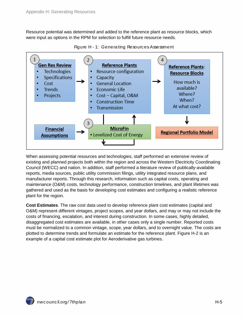
Appendix H: Generating Resources
nwcouncil.org/7thplan H-5
Resource potential was determined and added to the reference plant as resource blocks, which were input as options in the RPM for selection to fulfill future resource needs.
Figure H - 1: Generating Resources Assessment
When assessing potential resources and technologies, staff performed an extensive review of existing and planned projects both within the region and across the Western Electricity Coordinating Council (WECC) and nation. In addition, staff performed a literature review of publically-available reports, media sources, public utility commission filings, utility integrated resource plans, and manufacturer reports. Through this research, information such as capital costs, operating and maintenance (O&M) costs, technology performance, construction timelines, and plant lifetimes was gathered and used as the basis for developing cost estimates and configuring a realistic reference plant for the region.
Cost Estimates. The raw cost data used to develop reference plant cost estimates (capital and O&M) represent different vintages, project scopes, and year dollars, and may or may not include the costs of financing, escalation, and interest during construction. In some cases, highly detailed, disaggregated cost estimates are available, in other cases only a single number. Reported costs must be normalized to a common vintage, scope, year dollars, and to overnight value. The costs are plotted to determine trends and formulate an estimate for the reference plant. Figure H-2 is an example of a capital cost estimate plot for Aeroderivative gas turbines.

Appendix H: Generating Resources
nwcouncil.org/7thplan H-6
Figure H - 2: Capital Cost Estimate for Aeroderivative Gas Turbines
Several input characteristics are used to compute the levelized cost of energy and complete the assumptions for the reference plant. The capital and O&M cost are inputs to MicroFin, which calculates the levelized cost of the generating resource.
MicroFin. A financial revenue requirements model – MicroFin - was used to calculate the levelized fixed cost and the full levelized cost of energy (LCOE) for each reference plant. The finance model calculates the annual cash flows which will satisfy revenue requirements over the plant lifetime. The annual cash flows are compressed and discounted into a single dollar value – Net Present Value (NPV). The NPV is then converted into a level, annualized payment (like a home mortgage payment). Two important cost values are output from the model:
1. Levelized fixed cost ($ per kilowatt-year) represents the cost of building and maintaining a power plant over its lifetime and is a primary cost input to RPM.
2. LCOE ($ per megawatt-hour) is the cost per unit of energy the plant is expected to produce and which also includes variable costs such as fuel, and variable O&M.
The finance assumptions which are input to MicroFin have an impact on the resulting levelized costs. For example, each generating resource type has a set estimate for the overnight capital cost, regardless of who pays for the plant. However, the cost of capital to actually build the plant may vary based on the financial sponsor – such as a municipal or public utility, an investor-owned utility (IOU) or an independent power producer (IPP). Other important finance assumptions include the discount rate, rates of return, and investment tax credits. Important operating assumptions include gas price forecasts, O&M, and capacity factors. The financial assumptions for project sponsors are detailed in Table H-2 below.

Appendix H: Generating Resources
nwcouncil.org/7thplan H-7
Table H - 2: Financial Assumptions for Project Sponsors
Financial Investor Owned Utility* Independent Power Producer** Federal Income Tax 35 % 35 %
Federal Investment Tax Credit (ITC)
Solar: 30% through 2019, 26% in 2020, 22% in 2021, 10% in
2022 and thereafter
Geothermal: 10% State Tax 5 % 5 %
Property Tax 1.4 % 1.4 % Insurance 0.25 % 0.25 %
Debt Fraction 50 % 60 % Debt Term 25 – 30 years 20 years
Debt Interest Rate (nominal) 6.69 % 6.69 % Return On Equity (nominal) 10 % 12 %
Discount Rate 4 % 4 % * Wind and Gas Plants ** Utility Scale Solar and Geothermal
Quantifying Environmental Effects The Northwest Power Act requires the Council to estimate the incremental system cost of each new resource or conservation measure considered for inclusion in the plan’s new resource strategy.
Environmental standards, the actions required for compliance, and the associated costs vary by geographic location and by the circumstances of different resources. These are best represented in the Council’s planning process by representative plants characteristic of those that could be expected to be developed in the Northwest. With few exceptions, the sources of cost information for these plants available to the Council aggregate all of the costs of the plants, making it difficult to break out the embedded cost of environmental compliance. However, because the resource cost estimates are based on recently constructed or proposed plants, the Council assumes that the costs do include the cost of compliance with current and near-term planned environmental regulation.
Chapter 19 describes the Council’s methodology for quantifying environmental costs and benefits. Appendix I describes in detail the effects on the environment associated with different types of generating resources considered for inclusion in the power plan’s resource strategy, as well as the environmental regulations developed by other agencies of government to address those effects.
Resource Attributes The following attributes are used to describe the resource reference plants for the Seventh Power Plan. Note that all costs are expressed in constant 2012 year dollars.
Configuration. The number of units (and generating capacity of each unit) that make up the complete reference plant. Also includes the air emissions controls, cooling (wet vs. dry), and other plant specifications.

Appendix H: Generating Resources
nwcouncil.org/7thplan H-8
Location. The general geographic location of the reference plant, which is important in properly accounting for plant attributes (e.g. capacity factor) and costs (transmission).
Earliest In-Operation Date (Year). The earliest date a reference plant is assumed to be in operation, taking into account development and construction. The RPM cannot select the resource before this date.
Construction Lead Time. The amount of time it takes from project conception to commissioning. For the Seventh Power Plan, there are two phases:
Development Period (Years). Includes planning and development, from the identification of need (for example in a utility IRP) to establishment of the engineering, procuring, and construction (EPC) contract (which includes all siting and licensing, environmental assessments, and preliminary engineering).
Construction Period (Years). From the Notice to Proceed (NTP) to complete construction and commissioning.
Developable Potential. For modeling purposes in RPM, constraints were assigned to each reference plant. For some of the cases, the constraints on development are “soft”, meaning the constraint may not be a true limit on the potential development of that reference plant, but is merely an estimate of the number of plants that could be built at the modeled cost. In other cases, the constraints may be considered more “hard”, which could be caused by transmission capacity constraints at a given location.
Economic Life (Years). The assumed useful operating life of the plant.
Financial Sponsor. Power plants can be constructed by investor-owned utilities, consumer-owned utilities and independent power producer developers. Each of these entities uses different project financing mechanisms. The differing financing mechanisms and financial incentives available for some resources result in different total investment costs and annual capital service requirements for otherwise identical projects. See Table H-2 for details on project sponsors.
Capacity (MW). The lifecycle capacity in megawatts of the individual reference plant.
Capacity Factor (%). An estimate of the ratio of the actual annual output to the potential annual output if the plant is operated at full capacity. This is a useful value when looking at variable energy generation in different locations, such as wind and solar PV.
Fuel. The primary type of fuel burned (natural gas, oil, coal, etc.), its location of origin, and cost.
Heat Rate (Btu/kWh). A measure of the efficiency of which a generator converts fuel into electricity. Full load, net plant lifetime averages, expressed as higher heating values (HHV).
Overnight Capital Cost ($/kW). An estimate of the project development and construction cost. “Overnight” refers to what the cost would be if the plant were built instantly, or over one night. This cost constitutes a sum of the EPC costs, plus owner’s costs (costs incurred by the project developer – permits, licenses, land, project development costs, infrastructure, taxes, regulatory compliance costs, etc.).

Appendix H: Generating Resources
nwcouncil.org/7thplan H-9
All-In Capital Cost ($/kW). An estimate of the total investment cost related to capital, including the cost of securing financing, interest during construction, and escalation during construction.
Fixed O&M Cost ($/kW-yr). An estimate of the fixed operation and maintenance cost for the reference plant, including operating and maintenance, labor and materials, and administrative overhead. Both routine maintenance, and major maintenance and capital replacement are assumed to be included.
Variable O&M Cost ($/MWh). An estimate of the variable operation and maintenance cost for the reference plant, including all costs that are a function of the amount of power produced. This includes consumables such as water, chemicals, lubricants, and catalysts, and waste disposal.
Transmission. The assumed transmission (existing or new) that is incorporated into the cost of the resource.
Levelized Fixed Cost ($/kW-yr). An estimate of the cost of planning, building and maintaining a power plant over its lifetime, on an annualized cost basis.
Levelized Cost of Energy ($/MWh). An estimate of the cost per unit of energy for a resource over its productive lifetime, including fixed costs, and, under an assumed capacity factor, variable costs such as variable O&M and fuel commodity costs.
GENERATING RESOURCE REFERENCE PLANTS Combined Cycle Combustion Turbine Description of Reference Plant. Three reference plants based on two slightly different types of combined cycle combustion turbines technologies (CCCT) were developed. The first is based on the Siemens H-Class in a one gas turbine by one steam turbine configuration (1x1), utilizing wet cooling, and located on the East side of the Cascade mountains. The total baseload plant capacity is 370 megawatts and the heat rate is 6,770 British thermal units per kilowatt-hour. The second reference plant is based on the Mitsubishi Heavy Industries (MHI) J-Class in a one gas turbine by one steam turbine configuration (1x1), utilizing dry cooling, also located on the East side. The total plant capacity is slightly larger at 425 megawatts and the heat rate is 6,704 British thermal units per kilowatt-hour. The third reference plant is based on MHI J-Class but set on the West side. It is assumed that a new CCCT on the West side would require additional costs associated with pipeline expansion. Tables H-3 and H-4 provide a summary of the plants. For each plant, the Council’s medium natural gas price forecast was used for calculating the levelized cost of energy ($/MWh).1
Each plant is assumed to operate on natural gas supplied on a firm transportation contract. Location-specific adjustments were made for firm service cost estimates and for the impact of
1 Note that the levelized cost shown in Tables H-3 and H-4 are for narrative purposes only. The Regional Portfolio Model calculates a unique levelized cost for each resource based on the natural gas prices and capacity utilization simulated in each of the 800 futures tested in the model.

Appendix H: Generating Resources
nwcouncil.org/7thplan H-10
elevation on output. Emission controls include low-nitrogen oxide burners and selective catalytic reduction for nitrogen oxide control and an oxidation catalyst for carbon and volatile organic compound control. The financial assumptions used for calculating levelized costs were consistent with an IOU sponsor.
Importance/Relevance to PNW. Combined cycle combustion turbines are the largest and most efficient of the gas-fired generating technologies. These versatile plants have the ability to replace baseload coal power, can act as a firming resource for variable renewable generation, and fill in gaps from reduced hydro power production during low water years. CCCTs emit carbon dioxide at significantly lower rates than coal plants, and may play a key role in helping to reduce overall carbon dioxide emissions as proposed in the Federal Clean Power Plan. This technology also benefits from the robust existing natural gas infrastructure system in the region, as well as plentiful and low cost fuel supply.
Development potential. Overall, the potential for CCCT development in the region is large. For modeling purposes in RPM, the wet-cooled CCCT reference plant on the East side was limited to 1,110 MW of total development (three plants) to represent the possibility of permitting constraints for plants with heavy water usage. Dry cooled units on the East side have significant potential for development since the technology is not a heavy water consumer, and there is ample pipeline capacity on the East side. The potential for CCCT development may be more limited on the West side where potential constraints on pipeline capacity could hamper or delay development.

Appendix H: Generating Resources
nwcouncil.org/7thplan H-11
Table H - 3: CCCT Reference Plants
Reference Plant CCCT Adv 1 Wet Cool East
CCCT Adv 2 Dry Cool East
CCCT Adv 2 Dry Cool West
Configuration 1 gas turbine x 1
steam turbine and wet cooling system
1 gas turbine x 1 steam turbine and dry
cooling system
1 gas turbine x 1 steam turbine and dry
cooling system
Note
Based on Siemens H-Class. Number of
plants with wet cooling may be limited
Based on MHI J-Class
Based on MHI J-Class. Assumed to require
gas pipeline expansion on West side
Location East side East side West side Earliest In-Operation
Date 2020 2021 2021
Development Period (Years) 2 2 2
Construction Period (Years) 3 3 3
Economic Life (Years) 30 30 30 Financial Sponsor IOU IOU IOU
Capacity (MW) 370 425 426
Fuel Natural Gas East Natural Gas East Natural Gas West with pipeline expansion
Heat Rate (btu/kWh) 6,770 6,704 6,704 Overnight Capital Cost
($/kW) 1,147 1,287 1,282
Fixed O&M Cost ($/kW-yr) 15.37 15.37 15.37
Variable O&M Cost ($/MWh) 3.27 3.27 3.27
Transmission BPA point to point BPA point to point BPA point to point with transmission deferral
credit Maximum build-out (MW) as modeled 1,110 5,950 1,278
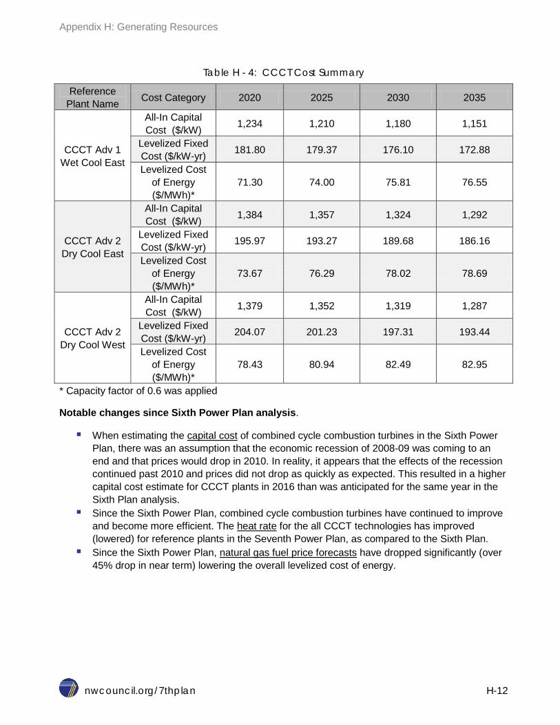
Appendix H: Generating Resources
nwcouncil.org/7thplan H-12
Table H - 4: CCCT Cost Summary
Reference Plant Name Cost Category 2020 2025 2030 2035
CCCT Adv 1 Wet Cool East
All-In Capital Cost ($/kW) 1,234 1,210 1,180 1,151
Levelized Fixed Cost ($/kW-yr) 181.80 179.37 176.10 172.88
Levelized Cost of Energy ($/MWh)*
71.30 74.00 75.81 76.55
CCCT Adv 2 Dry Cool East
All-In Capital Cost ($/kW) 1,384 1,357 1,324 1,292
Levelized Fixed Cost ($/kW-yr) 195.97 193.27 189.68 186.16
Levelized Cost of Energy ($/MWh)*
73.67 76.29 78.02 78.69
CCCT Adv 2 Dry Cool West
All-In Capital Cost ($/kW) 1,379 1,352 1,319 1,287
Levelized Fixed Cost ($/kW-yr) 204.07 201.23 197.31 193.44
Levelized Cost of Energy ($/MWh)*
78.43 80.94 82.49 82.95
* Capacity factor of 0.6 was applied
Notable changes since Sixth Power Plan analysis.
When estimating the capital cost of combined cycle combustion turbines in the Sixth Power Plan, there was an assumption that the economic recession of 2008-09 was coming to an end and that prices would drop in 2010. In reality, it appears that the effects of the recession continued past 2010 and prices did not drop as quickly as expected. This resulted in a higher capital cost estimate for CCCT plants in 2016 than was anticipated for the same year in the Sixth Plan analysis.
Since the Sixth Power Plan, combined cycle combustion turbines have continued to improve and become more efficient. The heat rate for the all CCCT technologies has improved (lowered) for reference plants in the Seventh Power Plan, as compared to the Sixth Plan.
Since the Sixth Power Plan, natural gas fuel price forecasts have dropped significantly (over 45% drop in near term) lowering the overall levelized cost of energy.

Appendix H: Generating Resources
nwcouncil.org/7thplan H-13
Reciprocating Engine Description of Reference Plant. The reciprocating engine reference plant is based off of the Wärtsilä 18V50SG natural gas engine with twelve, 18.3 megawatt modules. The total plant capacity is 220 megawatts and the heat rate is 8,370 British thermal units per kilowatt-hour. One reference plant is located on the East side, while two additional reference plants are located on the West side. West side reference plants were defined with and without expansion of the West side gas pipeline system. There is assumed to be sufficient natural gas capacity on the East side. A firm gas transport contract is assumed. Air emission controls include a combined selective catalytic reduction and oxidation catalyst to reduce nitrogen oxides (NOx), carbon monoxide (CO) and volatile organic compound (VOC) emissions. The financial assumptions used for calculating levelized costs were consistent with an IOU sponsor. Tables H-5 and H-6 provide a summary of the plants.
Importance/Relevance to PNW. Traditionally, gas peakers (primarily frame units) were used to help shape and firm hydroelectric power in the Pacific Northwest. Technological advancements in both reciprocating engines and simple cycle combustion turbines have resulted in more flexible and efficient machines with fast start times and rapid response to system changes, leading to the ability to help meet short-term peak loads and integrate variable energy generation. Reciprocating engine generating sets in particular have the benefit of being modular and able to size according to need, and are very efficient. They are also not as sensitive to temperatures or elevations in terms of output as the simple and combined cycle combustion turbines.
Development potential. Overall, the potential for reciprocating engine development in the region is large. The potential for development may be more limited on the West side where potential constraints on pipeline capacity could hamper or delay development.
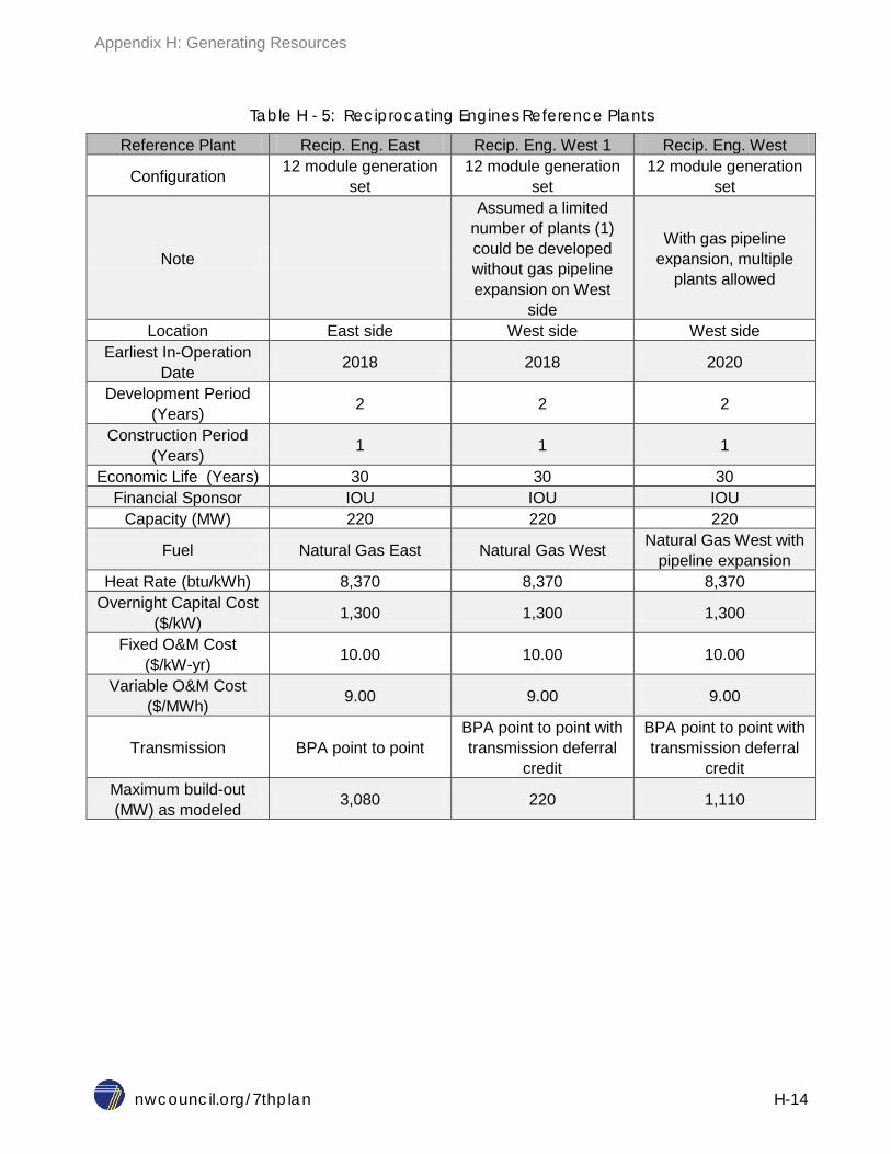
Appendix H: Generating Resources
nwcouncil.org/7thplan H-14
Table H - 5: Reciprocating Engines Reference Plants
Reference Plant Recip. Eng. East Recip. Eng. West 1 Recip. Eng. West
Configuration 12 module generation set
12 module generation set
12 module generation set
Note
Assumed a limited number of plants (1) could be developed without gas pipeline expansion on West
side
With gas pipeline expansion, multiple
plants allowed
Location East side West side West side Earliest In-Operation
Date 2018 2018 2020
Development Period (Years) 2 2 2
Construction Period (Years) 1 1 1
Economic Life (Years) 30 30 30 Financial Sponsor IOU IOU IOU
Capacity (MW) 220 220 220
Fuel Natural Gas East Natural Gas West Natural Gas West with pipeline expansion
Heat Rate (btu/kWh) 8,370 8,370 8,370 Overnight Capital Cost
($/kW) 1,300 1,300 1,300
Fixed O&M Cost ($/kW-yr) 10.00 10.00 10.00
Variable O&M Cost ($/MWh) 9.00 9.00 9.00
Transmission BPA point to point BPA point to point with transmission deferral
credit
BPA point to point with transmission deferral
credit Maximum build-out (MW) as modeled 3,080 220 1,110
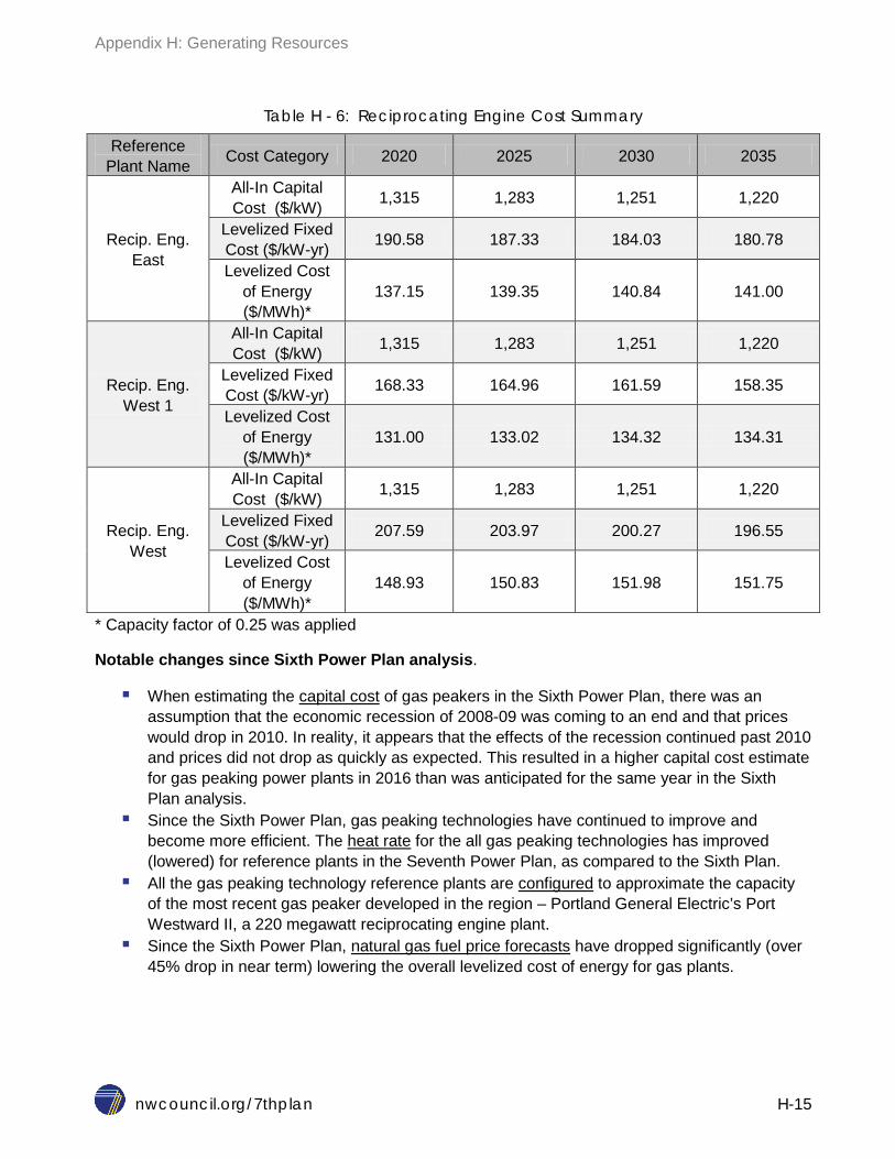
Appendix H: Generating Resources
nwcouncil.org/7thplan H-15
Table H - 6: Reciprocating Engine Cost Summary
Reference Plant Name Cost Category 2020 2025 2030 2035
Recip. Eng. East
All-In Capital Cost ($/kW) 1,315 1,283 1,251 1,220
Levelized Fixed Cost ($/kW-yr) 190.58 187.33 184.03 180.78
Levelized Cost of Energy ($/MWh)*
137.15 139.35 140.84 141.00
Recip. Eng. West 1
All-In Capital Cost ($/kW) 1,315 1,283 1,251 1,220
Levelized Fixed Cost ($/kW-yr) 168.33 164.96 161.59 158.35
Levelized Cost of Energy ($/MWh)*
131.00 133.02 134.32 134.31
Recip. Eng. West
All-In Capital Cost ($/kW) 1,315 1,283 1,251 1,220
Levelized Fixed Cost ($/kW-yr) 207.59 203.97 200.27 196.55
Levelized Cost of Energy ($/MWh)*
148.93 150.83 151.98 151.75
* Capacity factor of 0.25 was applied
Notable changes since Sixth Power Plan analysis.
When estimating the capital cost of gas peakers in the Sixth Power Plan, there was an assumption that the economic recession of 2008-09 was coming to an end and that prices would drop in 2010. In reality, it appears that the effects of the recession continued past 2010 and prices did not drop as quickly as expected. This resulted in a higher capital cost estimate for gas peaking power plants in 2016 than was anticipated for the same year in the Sixth Plan analysis.
Since the Sixth Power Plan, gas peaking technologies have continued to improve and become more efficient. The heat rate for the all gas peaking technologies has improved (lowered) for reference plants in the Seventh Power Plan, as compared to the Sixth Plan.
All the gas peaking technology reference plants are configured to approximate the capacity of the most recent gas peaker developed in the region – Portland General Electric’s Port Westward II, a 220 megawatt reciprocating engine plant.
Since the Sixth Power Plan, natural gas fuel price forecasts have dropped significantly (over 45% drop in near term) lowering the overall levelized cost of energy for gas plants.

Appendix H: Generating Resources
nwcouncil.org/7thplan H-16
Simple Cycle - Aeroderivative Gas Turbine Description of Reference Plant. The Aeroderivative gas turbine reference plant is based on the General Electric LM6000PF SPRINT, with four, 47 megawatt turbine generators. The total plant capacity is 178 megawatts and the heat rate is 9,477 British thermal units per kilowatt-hour. One reference plant is located on the East side, while two additional reference plants are located on the West side. West side reference plants were defined with and without new build out of the West side gas pipeline system. There is assumed to be sufficient natural gas capacity on the East side. Air emission controls include water injection and selective catalytic reduction for nitrogen oxide control and an oxidation catalyst for carbon and volatile organic compound reduction. The financial assumptions used for calculating levelized costs were consistent with an IOU sponsor. Tables H-7 and H-8 provide a summary of the plants.
Importance/Relevance to PNW. Traditionally, gas peakers (primarily frame units) were used to help shape and firm hydroelectric power in the Pacific Northwest. Technological advancements in both reciprocating engines and simple cycle combustion turbines have resulted in more flexible and efficient machines with fast start times and rapid response to system changes, leading to the ability to help meet short-term peak loads and integrate variable energy generation. Aeroderivative plants in particular have been popular developments in the Western Electricity Coordinating Council (WECC) region over the past decade.
Development potential. Overall, the potential for Aeroderivative gas turbine development in the region is large. The potential for development may be more limited on the West side where potential constraints on pipeline capacity could hamper or delay development.

Appendix H: Generating Resources
nwcouncil.org/7thplan H-17
Table H - 7: Aeroderivative Gas Turbine Reference Plants
Reference Plant Aero GT East Aero GT West 1 Aero GT West Configuration 4 GT x 47 MW 4 GT x 47 MW 4 GT x 47 MW
Note
Assumed a limited number of plants (1) could be developed without gas pipeline expansion on West
side
With gas pipeline expansion, multiple
plants allowed
Location East side West side West side Earliest In-Operation
Date 2018 2018 2020
Development Period (Years) 2 2 2
Construction Period (Years) 1 1 1
Economic Life (Years) 30 30 30 Financial Sponsor IOU IOU IOU
Capacity (MW) 178 179 179
Fuel Natural Gas East Natural Gas West Natural Gas West with pipeline expansion
Heat Rate (btu/kWh) 9,477 9,477 9,477 Overnight Capital Cost
($/kW) 1,111 1,107 1,107
Fixed O&M Cost ($/kW-yr) 25.00 25.00 25.00
Variable O&M Cost ($/MWh) 5.00 5.00 5.00
Transmission BPA point to point BPA point to point with transmission deferral
credit
BPA point to point with transmission deferral
credit Maximum build-out (MW) as modeled 2,492 179 1,074

Appendix H: Generating Resources
nwcouncil.org/7thplan H-18
Table H - 8: Aeroderivative Gas Turbine Cost Summary
Reference Plant Name Cost Category 2020 2025 2030 2035
Aero GT East
All-In Capital Cost ($/kW) 1,124 1,096 1,069 1,043
Levelized Fixed Cost ($/kW-yr) 191.76 188.58 185.32 181.99 Levelized Cost
of Energy ($/MWh)* 139.10 141.80 143.69 144.04
Aero GT West 1
All-In Capital Cost ($/kW) 1,120 1,092 1,065 1,039
Levelized Fixed Cost ($/kW-yr) 169.63 166.34 163.01 159.69
Levelized Cost of Energy ($/MWh)*
133.53 136.04 137.72 137.88
Aero GT West
All-In Capital Cost ($/kW) 1,120 1,092 1,065 1,039
Levelized Fixed Cost ($/kW-yr) 214.09 210.50 206.80 202.94
Levelized Cost of Energy ($/MWh)*
153.83 156.20 157.72 157.63
* Capacity Factor of 0.25 was applied
Notable changes since Sixth Power Plan analysis.
When estimating the capital cost of gas peakers in the Sixth Power Plan, there was an assumption that the economic recession of 2008-09 was coming to an end and that prices would drop in 2010. In reality, it appears that the effects of the recession continued past 2010 and prices did not drop as quickly as expected. This resulted in a higher capital cost estimate for gas peaking power plants in 2016 than was anticipated for the same year in the Sixth Plan analysis.
Since the Sixth Power Plan, gas peaking technologies have continued to improve and become more efficient. The heat rate for the all gas peaking technologies has improved (lowered) for reference plants in the Seventh Power Plan, as compared to the Sixth Plan.
All the gas peaking technology reference plants are configured to approximate the capacity of the most recent gas peaker developed in the region – Portland General Electric’s Port Westward II, a 220 megawatt reciprocating engine plant.
Since the Sixth Power Plan, natural gas fuel price forecasts have dropped significantly (over 45% drop in near term) lowering the overall levelized cost of energy for gas plants.

Appendix H: Generating Resources
nwcouncil.org/7thplan H-19
Simple Cycle - Frame Gas Turbine Description of Reference Plant. The frame gas turbine reference plant is based off of the General Electric 7F5S with one, 216 megawatt turbine generator. The total plant capacity is therefore 216 megawatts and the heat rate is 10,266 British thermal units per kilowatt-hour. One reference plant is located on the East side, while two additional reference plants are located on the West side. West side reference plants were defined with and without new build out of the West side gas pipeline system. There is assumed to be sufficient natural gas capacity on the East side. A firm gas transport contract is assumed. The financial assumptions used for calculating levelized costs were consistent with an IOU sponsor. Tables H-9 and H-10 provide a summary of the plants.
Importance/Relevance to PNW. Traditionally, gas peakers (primarily frame units) were used to help shape and firm hydroelectric power in the Pacific Northwest. Technological advancements in both reciprocating engines and simple cycle combustion turbines have resulted in more flexible and efficient machines with fast start times and rapid response to system changes, leading to the ability to help meet short-term peak loads and integrate variable energy generation. The frame gas turbine plant has lower upfront capital costs than the Aeroderivative, but runs at a lower efficiency and is less flexible.
Development potential. Overall, the potential for frame gas turbine development in the region is large. The potential for development may be more limited on the West side where potential constraints on pipeline capacity could hamper or delay development.

Appendix H: Generating Resources
nwcouncil.org/7thplan H-20
Table H - 9: Frame Gas Turbine Reference Plants
Reference Plant Frame GT East Frame GT West 1 Frame GT West Configuration 1 GT x 216 MW 1 GT x 216 MW 1 GT x 216 MW
Note
Assumed a limited number of plants (1) could be developed without gas pipeline expansion on West
side
With gas pipeline expansion, multiple
plants allowed
Location East side West side West side Earliest In-Operation
Date 2018 2018 2020
Development Period (Years) 2 2 2
Construction Period (Years) 1 1 1
Economic Life (Years) 30 30 30 Financial Sponsor IOU IOU IOU
Capacity (MW) 200 201 201
Fuel Natural Gas East Natural Gas West Natural Gas West with pipeline expansion
Heat Rate (btu/kWh) 10,266 10,266 10,266 Overnight Capital Cost
($/kW) 808 805 805
Fixed O&M Cost ($/kW-yr) 7.00 7.00 7.00
Variable O&M Cost ($/MWh) 10.00 10.00 10.00
Transmission BPA point to point BPA point to point with transmission deferral
credit
BPA point to point with transmission deferral
credit Maximum build-out (MW) as modeled 2,800 201 1,005

Appendix H: Generating Resources
nwcouncil.org/7thplan H-21
Table H - 10: Frame Gas Turbine Cost Summary
Reference Plant Name Cost Category 2020 2025 2030 2035
Frame GT East
All-In Capital Cost ($/kW) 817 797 777 758
Levelized Fixed Cost ($/kW-yr) 147.64 145.49 143.26 140.95
Levelized Cost of Energy ($/MWh)*
127.83 131.37 134.02 134.98
Frame GT West 1
All-In Capital Cost ($/kW) 814 794 775 755
Levelized Fixed Cost ($/kW-yr) 125.97 123.70 121.40 119.10
Levelized Cost of Energy ($/MWh)*
122.85 126.81 128.61 129.36
Frame GT West
All-In Capital Cost ($/kW) 814 794 775 755
Levelized Fixed Cost ($/kW-yr) 174.13 171.54 168.84 165.95
Levelized Cost of Energy ($/MWh)*
144.84 148.02 150.27 150.75
* Capacity factor of 0.25 was applied
Notable changes since Sixth Power Plan analysis.
When estimating the capital cost of gas peakers in the Sixth Power Plan, there was an assumption that the economic recession of 2008-09 was coming to an end and that prices would drop in 2010. In reality, it appears that the effects of the recession continued past 2010 and prices did not drop as quickly as expected. This resulted in a higher capital cost estimate for gas peaking power plants in 2016 than was anticipated for the same year in the Sixth Plan analysis.
Since the Sixth Power Plan, gas peaking technologies have continued to improve and become more efficient. The heat rate for the all gas peaking technologies has improved (lowered) for reference plants in the Seventh Power Plan, as compared to the Sixth Plan.
All the gas peaking technology reference plants are configured to approximate the capacity of the most recent gas peaker developed in the region – Portland General Electric’s Port Westward II, a 220 megawatt reciprocating engine plant.
Since the Sixth Power Plan, natural gas fuel price forecasts have dropped significantly (over 45% drop in near term) lowering the overall levelized cost of energy for gas plants.

Appendix H: Generating Resources
nwcouncil.org/7thplan H-22
Utility-Scale Solar Photovoltaic Description of Reference Plants. Five reference plants were defined for utility scale solar. All of the plant capacities are defined in terms of megawatts (alternating current - AC) configured with crystalline silicon based modules mounted on single-axis trackers. The reference plants are modeled to have a 30-year lifetime with an annual degradation of one percent. To be consistent with utility scale solar development across the US, the project sponsor was assumed to be an independent power producer. Due to the rapidly changing cost environment for solar technology, a forecast of capital costs was developed, along with a low and high cost range. The first solar PV reference plant is a 20 megawatt (AC) plant located in Southern Idaho and is based on the mid-range capital cost estimate. Another larger plant, 50 megawatt (AC), is in the same location but with the low range estimated capital and O&M cost. The third reference plant located in Southern Idaho contains an estimate for additional transmission related costs to bring the power to the West side. Two reference plants were defined for the West side, where the solar resource is not as favorable, but transmission is available. The medium and the low capital cost estimates were used to define these plants. Tables H-11 and H-12 provide a summary.
Importance/Relevance to PNW. Although current presence in the region is limited, activity has recently picked up in Southern Idaho. As solar installation costs continue to decline, solar power may become more significant to the region; although without storage capability, solar power remains a variable energy resource which does not contribute to peak capacity in the winter.
Development potential. The potential for utility scale solar development in the region is large, particularly in Southern Idaho where the best capacity factors could be achieved. Limited existing transmission capacity from Southern Idaho to the West side load centers could create a hurdle for more extensive development. Should installation costs continue to decline, significant solar development could also occur in Western Oregon and Washington where transmission may be more readily available.

Appendix H: Generating Resources
nwcouncil.org/7thplan H-23
Table H - 11: Solar PV Reference Plants
Reference Plant Solar PV S. ID Solar PV S. ID w/
Transmission Expansion
Solar PV Low Cost S. ID
Solar PV W. WA
Solar PV Low Cost W. WA
Configuration
20 MWac installation with
crystalline silicon panels
and single axis tracker system
20 MWac installation with
crystalline silicon panels and single
axis tracker system
50 MWac installation with
crystalline silicon panels
and single axis tracker system
50 MWac installation
with crystalline
silicon panels and single
axis tracker system
50 MWac installation with
crystalline silicon panels and single
axis tracker system
Note Mid-range capital cost estimate
Mid-range capital cost estimate
Low range capital cost
estimate
Mid-range capital cost
estimate
Low range capital cost estimate
Location Southern Idaho Southern Idaho Southern Idaho Western WA Western WA
Earliest In-Operation Date
2018 2021 2020 2020 2020
Development Period (Years)
2 2 2 2 2
Construction Period (Years)
1 1 1 1 1
Economic Life (Years) 30 30 30 30 30
Financial Sponsor IPP IPP IPP IPP IPP
Investment Tax Credit* 30%/10 % 30%/10 % 30%/10 % 30%/10 % 30%/10 %
Capacity (MW) 17.4 17.4 48 48 48
Capacity Factor 0.26 0.26 0.26 0.19 0.19
Overnight Capital Cost ($/kW)
2,413 2,413 1,685 2,413 1,685
Fixed O&M Cost ($/kW-yr)
16.63 16.63 11.62 16.63 11.62
Variable O&M Cost ($/MWh)
0 0 0 0 0
Transmission Idaho Power Transmission
Expansion & BPA Idaho Power
BPA point to point
BPA point to point
Maximum build-out (MW) as modeled
642 989 642 3840 3840
* ITC at 30% through year 2019, stepping down to 10% in 2022
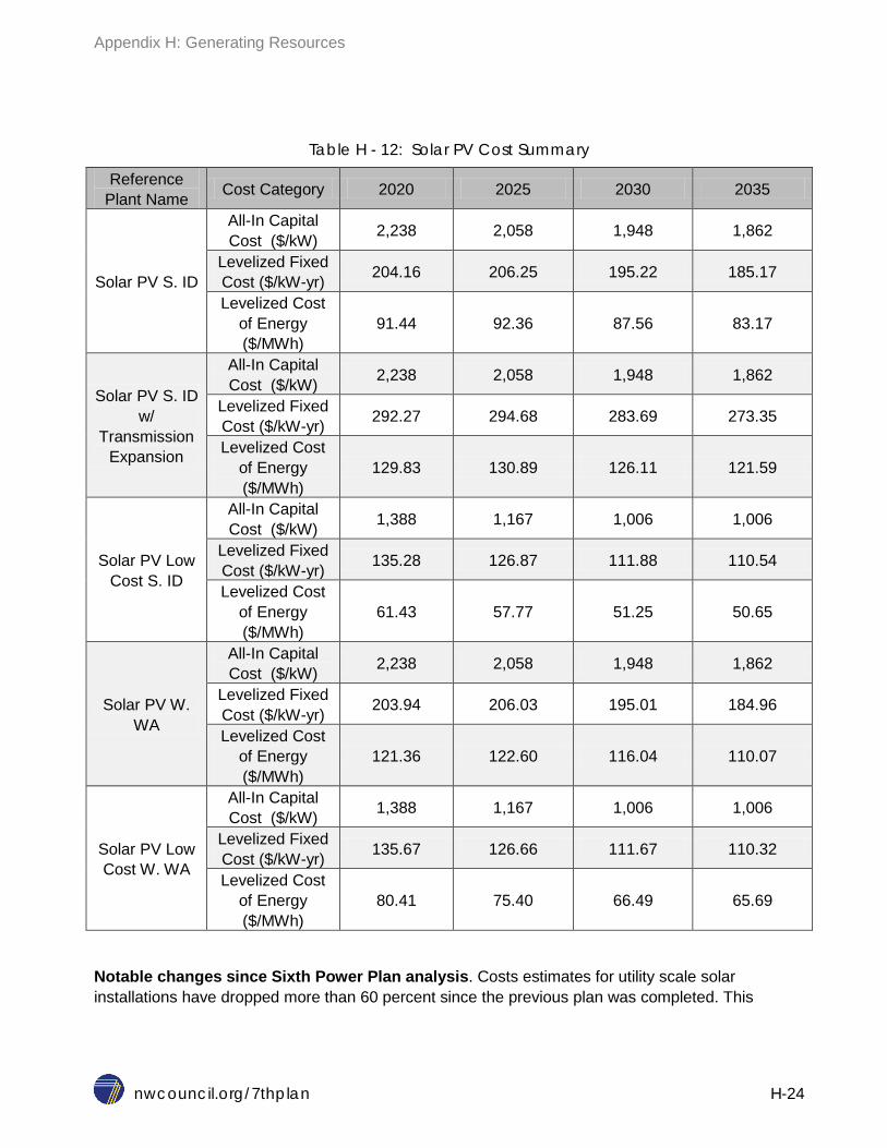
Appendix H: Generating Resources
nwcouncil.org/7thplan H-24
Table H - 12: Solar PV Cost Summary
Reference Plant Name Cost Category 2020 2025 2030 2035
Solar PV S. ID
All-In Capital Cost ($/kW) 2,238 2,058 1,948 1,862
Levelized Fixed Cost ($/kW-yr) 204.16 206.25 195.22 185.17
Levelized Cost of Energy ($/MWh)
91.44 92.36 87.56 83.17
Solar PV S. ID w/
Transmission Expansion
All-In Capital Cost ($/kW) 2,238 2,058 1,948 1,862
Levelized Fixed Cost ($/kW-yr) 292.27 294.68 283.69 273.35
Levelized Cost of Energy ($/MWh)
129.83 130.89 126.11 121.59
Solar PV Low Cost S. ID
All-In Capital Cost ($/kW) 1,388 1,167 1,006 1,006
Levelized Fixed Cost ($/kW-yr) 135.28 126.87 111.88 110.54
Levelized Cost of Energy ($/MWh)
61.43 57.77 51.25 50.65
Solar PV W. WA
All-In Capital Cost ($/kW) 2,238 2,058 1,948 1,862
Levelized Fixed Cost ($/kW-yr) 203.94 206.03 195.01 184.96
Levelized Cost of Energy ($/MWh)
121.36 122.60 116.04 110.07
Solar PV Low Cost W. WA
All-In Capital Cost ($/kW) 1,388 1,167 1,006 1,006
Levelized Fixed Cost ($/kW-yr) 135.67 126.66 111.67 110.32
Levelized Cost of Energy ($/MWh)
80.41 75.40 66.49 65.69
Notable changes since Sixth Power Plan analysis. Costs estimates for utility scale solar installations have dropped more than 60 percent since the previous plan was completed. This

Appendix H: Generating Resources
nwcouncil.org/7thplan H-25
resulted in including solar PV as an input to RPM in the Seventh Power Plan, whereas in the previous plan it was not included.
Solar performance was simulated for the reference plant in Southern Idaho using the Solar Advisor Model (SAM), available on the NREL website.2 This model calculates hourly electricity output from a user-supplied, modeled photovoltaic system based on historic weather for a specific location. The Boise Airport location was used to represent Southern Idaho, along with the reference plant configuration. The simulated generation from the reference plant over a dozen years is shown in Figure H-3. In this case, the monthly capacity factor was calculated for individual weather years, as well as a typical meteorological year (TMY). The TMY uses actual weather data from the years of 1961 through 1990 to create a single annual representative series. This weather time series is useful for determining the expected average output of a specified system.
Figure H – 3: Simulated Monthly Solar Plant Output for Southern Idaho
As can be seen from the figure, the best solar output occurs in the months of April (4) through October (10). Output peaks in July (7), and on a year to year basis, July also provides the least amount of variation in terms of monthly output.
Wind Power: Utility Scale, Onshore Description of Reference Plant. The wind power reference plant consists of forty, 2.5 megawatt conventional three-blade wind turbine generators, creating a total plant installed nameplate capacity of 100 megawatts. The plant is assumed to include in-plant electrical and control systems,
2 https://sam.nrel.gov/
0.00
0.05
0.10
0.15
0.20
0.25
0.30
0.35
0.40
0.45
1 2 3 4 5 6 7 8 9 10 11 12
Capa
city
Fact
or
Month
Typical Meteorological Year
1964
1968
1970
1972
1975
1977
1978
1981
1983
1987
1988
1989

Appendix H: Generating Resources
nwcouncil.org/7thplan H-26
interconnection facilities and on-site roads, meteorological towers and support facilities. One reference plant is located in the Columbia Basin, while an additional four reference plants are located in central Montana with various transmission requirements. The financial assumptions used for calculating levelized costs were consistent with an IOU sponsor. Tables H-13 and H-14 provide a summary of the plants.
Importance/Relevance to PNW. Wind power has played a significant role in the region over the past decade. With the Renewable Portfolio Standards enacted by Oregon, Washington, Montana, and others in WECC, federal incentives, and PURPA projects spurring development in the Pacific Northwest, the region has installed about 7,500 megawatts capacity (~8,500 megawatts when including the PacifiCorp Wyoming projects). There has been a significant lull in wind development since the boom in 2012, due in part to uncertainty over federal tax incentives, but also due to utilities reaching their near-term RPS goals. As the next round of goals approaches in 2020, the region is likely to undergo another development of renewable resources, including wind power.
Developable potential. The potential for wind development in the region is large, particularly in the Columbia Basin where transmission is available. Locations in Montana have a robust wind resource, but lack substantial transmission to transfer power to the West side load centers. Transmission upgrades may be required before extensive wind development could take place in Montana.

Appendix H: Generating Resources
nwcouncil.org/7thplan H-27
Table H - 13: Wind Power Reference Plants
Reference Plant
Wind Columbia
Basin
Wind MT w/existing
Transmission
Wind MT w/ new
Transmission
Wind MT w/ Transmission
Upgrade
Wind MT w/ Colstrip
Transmission
Configuration 40 x 2.5 MW wind turbine generators
40 x 2.5 MW wind turbine generators
40 x 2.5 MW wind turbine generators
40 x 2.5 MW wind turbine generators
40 x 2.5 MW wind turbine generators
Note
Very limited transmission available to
bring to Western load
centers
New 230kV transmission line rolled into
capital cost
New 230kV transmission
line and Path 8 Upgrade
Using Colstrip
Transmission
Location OR/WA MT MT MT MT Earliest In-
Operation Date 2019 2019 2020 2020 n/a
Development Period (Years) 2 2 2 2 2
Construction Period (Years) 2 2 2 2 2
Economic Life (Years) 25 25 25 25 25
Financial Sponsor IOU IOU IOU IOU IOU
Capacity (MW) 100 100 100 100 100 Capacity Factor 0.32 0.40 0.40 0.40 0.40
Overnight Capital Cost
($/kW) 2,240 2,240 2,349 2,349 2,240
Fixed O&M Cost ($/kW-yr) 35.00 35.00 35.00 35.00 35.00
Variable O&M Cost ($/MWh) 2.00 2.00 2.00 2.00 2.00
Transmission BPA point to point
NorthWestern Energy, Montana
Intertie, BPA
NorthWestern Energy, Montana
Intertie, BPA
NorthWestern Energy, Montana
Intertie, BPA
Colstrip Trans.
System, Montana
Intertie, BPA Maximum build-
out (MW) as modeled
6,500 100 200 900 2000

Appendix H: Generating Resources
nwcouncil.org/7thplan H-28
Table H - 14: Wind Power Cost Summary
Reference Plant Name Cost Category 2020 2025 2030 2035
Wind Columbia
Basin
All-In Capital Cost ($/kW) 2,307 2,250 2,194 2,140
Levelized Fixed Cost ($/kW-yr) 303.39 297.50 291.65 286.08
Levelized Cost of Energy ($/MWh)
110.33 108.24 106.16 104.17
Wind MT w/existing
Transmission
All-In Capital Cost ($/kW) 2,307 2,250 2,194 2,140
Levelized Fixed Cost ($/kW-yr) 351.56 345.82 340.04 334.34
Levelized Cost of Energy ($/MWh)
102.45 100.82 99.18 97.55
Wind MT w/ new
Transmission
All-In Capital Cost ($/kW) 2,419 2,359 2,301 2,245
Levelized Fixed Cost ($/kW-yr) 363.04 357.04 351.00 345.07
Levelized Cost of Energy ($/MWh)
105.73 104.02 102.31 100.61
Wind MT w/ Transmission
Upgrade
All-In Capital Cost ($/kW) 2,419 2,359 2,301 2,245
Levelized Fixed Cost ($/kW-yr) 375.54 369.59 363.59 357.65
Levelized Cost of Energy ($/MWh)
109.29 107.61 105.90 104.20
Wind MT w/ Colstrip
Transmission
All-In Capital Cost ($/kW) 2,307 2,250 2,194 2,140
Levelized Fixed Cost ($/kW-yr) 322.50 316.63 310.77 305.12
Levelized Cost of Energy ($/MWh)
94.16 92.49 90.82 89.21
Notable changes since Sixth Power Plan analysis.
When estimating the capital cost of wind power plants in the Sixth Power Plan, there was an assumption that the economic recession of 2008-09 was coming to an end and that prices would drop in 2010. In reality, it appears that the effects of the recession continued past 2010

Appendix H: Generating Resources
nwcouncil.org/7thplan H-29
and prices did not drop as quickly as expected. This resulted in a higher capital cost estimate for wind power plants in 2016 than was anticipated for the same year in the Sixth Plan analysis.
As wind turbine technology has improved, so too have capacity factors. Hub heights have increased and improved the ability of the turbines to achieve a greater wind sweep area. There is also more real world data available to analyze what annual capacity factors are being achieved in certain areas. The estimated capacity factor for the reference wind power plants in Montana was improved from 38 percent in the Sixth Power Plan, to 40 percent in the Seventh Power Plan. The estimated capacity factor for the Columbia Gorge area remained unchanged at 32 percent due to previous build-out of the better wind resource sites.
The economic life of wind power plants was 20 years in the Sixth Plan, and has been increased to 25 years in the Seventh Power Plan based on real world examples, power purchase agreements, and utility IRP assumptions.
In the Sixth Power Plan, the federal Production Tax Credit (PTC) was incorporated in the levelized cost calculation. For the Seventh Power Plan, the levelized costs for each wind resource were developed assuming that the PTC would not be renewed after its expiration in 2014 (and therefore not included). Although the PTC has since been renewed by the Consolidated Appropriations Act in December 2015, the levelized costs for wind remain nearly unchanged even with the PTC included. This is because the renewed PTC expires at the end of 2019, before the anticipated need to construct new wind resources.
Geothermal: Conventional Description of Reference Plant. The conventional geothermal reference plant consists of three, 13 megawatt units, creating a total plant installed nameplate capacity of 39 megawatts. The plant is assumed to use closed-loop organic Rankine cycle binary technology suitable for low geothermal fluid temperatures. The plant includes production and injection wells, geothermal fluid piping, power block, cooling towers, step-up transformers, switchgear and interconnection facilities, and security, control, and maintenance facilities. Wet cooling, resulting in higher plant efficiency, greater productivity, and lower cost, would likely be used at sites with sufficient water. Dry cooling could be employed at sites with insufficient cooling water availability, at additional cost and some sacrifice in efficiency and productivity. The reference plant is located in Central Oregon, with existing transmission. The financial assumptions used for calculating levelized costs are consistent with an IPP sponsor. Tables H-15 and H-16 provide a summary of the plant.
Importance/Relevance to PNW. While wind power has been the dominant renewable resource in the Pacific Northwest over the past decade or so, other renewables are emerging and gaining appeal. With steadily declining capital costs, solar PV – a central renewable in the desert Southwest and California – is attracting interest in the region. Both wind and solar PV are variable energy resources and therefore not dispatchable on demand to the power system. Geothermal on the other hand, is capable of providing baseload, dispatchable energy, making it an attractive alternative to both renewable resources to help meet RPS goals and to thermal resources to contribute to baseload.

Appendix H: Generating Resources
nwcouncil.org/7thplan H-30
Developable potential. The Pacific Northwest has considerable potential for geothermal development, although to date there have been limited successful installations. A 2008 U.S. Geological Survey assessment3 of moderate (90° to 150° Celsius) and high (greater than 150° Celsius) temperature hydrothermal resource (with naturally occurring fluid, heat, and permeability) identified roughly 266 megawatts-equivalent (MWe)4 from currently known resources and an additional 1,103 MWe from undiscovered (modeled using GIS to determine “the spatial correlation of geological factors that facilitate the formation of geothermal systems5”) resources at 95% confidence6 in the four Northwest states. The study notes that at a 50% confidence factor, the potential increases to 839 MWe identified and 3,593 MWe undiscovered conventional geothermal resource.
For modeling purposes, staff is assuming that there are 475 megawatts conventional geothermal potential available during the planning period. When rounding the number out to even reference plants, the potential for the model is 468 megawatts (or twelve plants at 39 megawatts capacity). This estimate was based off of the identified geothermal potential in the USGS assessment (266 MWe = 293 MW capacity at 95 percent confidence) plus a percentage (15%) of the undiscovered potential (1103 MWe = 1213 MW * 0.15 = 182 MW). The 15 percent discount of the undiscovered potential takes into account the limited development in the Northwest to date, the high frequency of dry holes encountered during earlier attempts to develop Northwest geothermal resources, the high risk and long lead time, and the relatively few sites currently under exploration/development. While this estimate of potential for the plan is likely optimistic in terms of actual development, it is useful to include in the model as an option and can be viewed as a proxy for a low-cost, dispatchable renewable resource.
3 United States Geological Survey. Assessment of Moderate- and High-Temperature Geothermal Resources of the United States. 2008. 4 In this study, one MWe is defined as the capability of generating 8.77 gigawatt hours (one average megawatt) continuously for a period of 30 years (the assumed lifetime of the resource). 5 United States Geological Survey. Assessment of Moderate- and High-Temperature Geothermal Resources of the United States. 2008. 6 There is a 95% probability that at least the potential amount identified could be successfully extracted (high confidence).

Appendix H: Generating Resources
nwcouncil.org/7thplan H-31
Table H - 15: Conventional Geothermal Reference Plants
Reference Plant
Conventional Geothermal
Configuration 3 X 13.3 MW units Note 10% ITC applied
Location C. Oregon Earliest In-
Operation Date 2021
Development Period (Years) 4
Construction Period (Years) 2
Economic Life (Years) 30
Financial Sponsor IPP
Capacity (MW) 39 Capacity Factor 90%
Overnight Capital Cost
($/kW) 4,302
Fixed O&M Cost ($/kW-yr) 196.00
Variable O&M Cost ($/MWh) 5.00
Transmission BPA point to point Maximum build-
out (MW) as modeled
468
Table H - 16: Conventional Geothermal Cost Summary
Reference Plant Name Cost Category 2020 2025 2030 2035
Conventional Geothermal
All-In Capital Cost ($/kW) 4827 4709 4594 4483
Levelized Fixed Cost ($/kW-yr) 633.31 617.68 600.24 579.64
Levelized Cost of Energy ($/MWh)
85.44 83.48 81.28 78.65

Appendix H: Generating Resources
nwcouncil.org/7thplan H-32
Notable changes since Sixth Power Plan analysis.
The Seventh Plan estimate of capital cost for a conventional geothermal plant is based on the Sixth Plan analysis, plus a review of estimates from recent publications. The Sixth Plan estimate was based on a sample of as-built and preconstruction estimates, plus generic reported estimates of development costs. There is still a wide range in capital cost estimates as costs can be site specific.
The estimated capacity factor for the conventional geothermal reference plant has remained at 90 percent. As geothermal is a dispatchable resource that is available 24 hours a day regardless of variations in weather and climate, its capacity factor can be viewed more like an availability factor, similar to other baseload resources like natural gas.
The economic life of a conventional geothermal plant is estimated to remain at 30 years. In the Sixth Power Plan, the federal Investment Tax Credit (ITC) was incorporated in the
levelized cost calculation and is included again in the Seventh Power Plan. The ITC was renewed in December 2015 at 10% indefinitely (no stated expiration date) through the Consolidated Appropriations Act.
Transmission The common point of reference for the costs of new generating resources is the wholesale delivery point to local load serving areas. Estimates for the costs of transmission from the point of the generating project interconnection to the wholesale point of delivery are included in the overall estimated generating resource cost. Oregon and Washington resources serving Oregon and Washington loads include the Bonneville Power Administration transmission rate for long term, firm point to point transmission of $20/kW-year. Integration rates for variable resources such as wind ($14.76/kW-year) and solar ($2.52/kW-year)7 were included when appropriate for the wind and solar generating resources.
In working up the generation models for utility-scale solar in Southern Idaho, two cases were developed. For existing transmission capacity (Solar PV S. ID), the Idaho Power transmission rates ($22.71/kW-yr) were used, including an estimate for solar integration8 ($2.50/MWh). In order to bring additional solar power from Southern Idaho to the Western load centers in Oregon and Washington, new transmission may be required. The cost of new transmission for this case (Solar PV S. ID w/Trans. Expan.) was estimated using a proposed transmission project - B2H Boardman to Hemingway9 - as a proxy.
The amount of transmission capacity which could bring wind power from Montana to the Western load centers in Oregon and Washington is limited. Investments in future transmission projects and upgrades may be required for significant quantities of wind power to reach the West. One reference
7 http://www.bpa.gov/Finance/RateInformation/RatesInfoTransmission/2014%20Rate%20Schedule%20Summary_10-01-13.pdf 8 https://www.idahopower.com/pdfs/AboutUs/PlanningForFuture/solar/SolarIntegrationStudy.pdf 9 https://www.wecc.biz/TransmissionExpansionPlanning/Lists/Project

Appendix H: Generating Resources
nwcouncil.org/7thplan H-33
case for Montana wind was estimated with existing transmission, and three Montana wind reference cases were developed which include cost estimates of new or expanded transmission. The existing transmission case (Wind MT w/existing Trans.) includes transmission rates for NorthWestern Energy Transmission10, BPA IM-14 Montana Intertie, and BPA Point to Point Transmission. The second reference case (Wind MT w/new Trans.) has an estimate for a new 230kV line included in the cost, in addition to the existing transmission path. The third case (Wind MT w/Trans. Upgrade) includes the new 230kV line estimate in combination with an estimate of the proposed Path 8/CTS11 upgrade which could relieve congestion on Path 8 and provide additional transmission for renewable power from Broadview Montana to the Mid-Columbia area. The final Montana wind case (Wind MT w/Colstrip Transmission) includes estimated costs of existing transmission CTS, BPA IM-14 Montana Intertie, and BPA Point to Point Transmission if CTS transmission was available for wind.
Long-term Resource: Utility-Scale Solar PV + Battery Energy Storage System The pairing of solar with battery storage could provide additional benefits over solar alone, and has the potential to create a firm, dispatchable source of renewable energy. For example, during the day dynamic cloud conditions can hamper solar PV electricity generation, resulting in variable output. An integrated battery energy storage system (BESS) could smooth the solar output to provide a steadier source of electricity. With an integrated BESS, a solar PV plant could deliver electricity over a wider range of hours, such as in the evening or nighttime. By strategically charging a battery system during the day when solar production is high, storing the energy and discharging the battery in the evening or night, a solar PV plant could cover an expanded range of load conditions. Separately, solar technologies and battery energy storage technologies have been declining in terms of cost. These technologies have been installed as stand-alone systems, but efforts may be converging to install combined solar and battery systems on utility-scale levels. For example, the Kauai Island Utility Cooperative in Hawaii has signed a deal with SolarCity to purchase power from a proposed, fully-dispatchable utility scale solar facility which could deliver electricity in the night time.12
Figure H - 4 displays an example of a modeled utility scale solar PV plant coupled with an integrated battery energy storage system. The solar PV plant in the example is modeled as a grid-connected, 48 megawatt (alternating current) single-axis tracker plant in Western Washington. The battery storage system is modeled as a ten megawatt Lithium-ion system with discharge capability of up to four hours. The chart shows how the solar PV and storage system might be utilized over a winter day in order to provide generation after the sun has set. The grey line shows a typical hourly load pattern for a winter day in the region with peaks in the morning and evening. The dashed yellow line displays the expected solar PV generation, with peak generation in the early afternoon and dropping to zero in the early evening. In this single day example, the battery storage system could be charged
10 http://www.oasis.oati.com/NWMT/NWMTdocs/Schedule_7_-_Firm_PTP_Transmission_Service.pdf 11 https://www.wecc.biz/TransmissionExpansionPlanning/Lists/Project 12 http://www.bizjournals.com/pacific/news/2015/09/09/kauai-utility-signs-deal-with-solarcity-on-energy.html

Appendix H: Generating Resources
nwcouncil.org/7thplan H-34
in the afternoon using solar PV generation, and discharged in the evening time to provide output for the evening peak load. The orange line shows the overall system output.
Figure H - 4: Modeled Example of Solar + Battery System
The U.S. Department of Energy has developed near-term and long-term cost and performance targets for battery systems, including lithium-ion, flow, and other battery technologies. The near-term capital cost target is $1,750 per kilowatt, and the longer term target is $1,250 per kilowatt.13 Currently, lithium-ion systems fall in a cost range from around $2,000 to $4,000 per kilowatt.14 In the 2013 Portland General Electric Integrated Resource Plan, an estimate of the capital costs for a lithium-ion battery system came in at $2,380 per kilowatt15.
This information was used to develop a cost estimate for a potential combined solar + battery system. The modeled system is comprised of a 48 megawatt (alternating current) utility-scale solar plant and a 10 megawatt Lithium-ion battery energy storage system. As shown in Figure H – 4, the plant is assumed to utilize its own solar generation to charge the battery system during the day, and discharge the battery system in the evening after sunset. The battery system is assumed to have an 85 percent round trip efficiency, meaning for every 0.85 megawatt-hour the battery delivers to the grid, 1.0 megawatt-hour of solar generation was consumed to charge the system. In addition, in order to prolong battery life, the minimum charge level of the battery was assumed to be ten percent. Starting in the year 2020, the capital cost estimate for the battery system was $2,380 per kilowatt, and was modeled to decline to $1,750 per kilowatt by year 2025 and $1,250 per kilowatt by the year
13 Grid Energy Storage, U.S. Department of Energy, December 2013 14 DOE/EPRI Electricity Storage Handbook, February 2015 15 https://www.portlandgeneral.com/our_company/energy_strategy/resource_planning/docs/2013_irp_appG.pdf
0.0
0.2
0.4
0.6
0.8
1.0
1.2
-5
0
5
10
15
20
25
1 2 3 4 5 6 7 8 9 10 11 12 1 2 3 4 5 6 7 8 9 10 11 24
Load
Pro
file
Inde
x
MW
Hour of Day
Baseline Solar Generation Battery Charge
Battery Discharge Solar & Storage System Output
Load Profile

Appendix H: Generating Resources
nwcouncil.org/7thplan H-35
2030. The Investment Tax Credit of 30 percent through 2019 (and stepping down to ten percent thereafter) was applied to the entire project, since the battery was assumed to be charged by the solar plant. An estimate was made for both the medium and low cost solar reference plant estimates. The cost estimate did not include a solar specific battery management system due to a lack of information. Such management systems may be necessary to optimally integrate the solar plant with the battery. The cost assumptions by year for the solar plant alone are listed in Table H – 17 while the assumptions for the Lithium-ion battery system are listed in Table H-18. Finally, Table H-19 displays the resulting capital, fixed O&M, and levelized cost estimates for the combined solar + battery storage system by year. Because this is an emerging technology, the reference plants were not input to RPM.
Table H - 17: Utility Scale Solar PV Plant
Configuration Cost Estimate
Cost Category 2020 2025 2030 2035
48 MWac installation
with crystalline
silicon panels and single axis tracker
system located in Western
Washington
Mid range capital cost
estimate
Overnight Capital
Cost $/kW 2,162 1,988 1,882 1,799
Fixed O&M
$/kW-year 14.90 13.71 12.97 12.40
Low range capital cost
estimate
Overnight Capital
Cost $/kW 1,341 1,127 972 972
Fixed O&M
$/kW-year 9.24 7.77 6.70 6.70
Table H - 18: Lithium Ion Battery Storage System
Configuration Cost Category 2020 2025 2030 2035 10 MWac
Lithium-Ion battery system
with 85% round trip
efficiency and 10% minimum
state of charge
Overnight Capital Cost
$/kW 2,380 1,750 1,250 1,250
Fixed O&M $/kW-year 10.00 7.35 5.25 5.25

Appendix H: Generating Resources
nwcouncil.org/7thplan H-36
Table H - 19: Cost estimate for combined Utility Scale Solar PV + Lithium Ion Battery Storage System
Configuration Cost Estimate
Cost Category 2020 2025 2030 2035
48 MWac solar installation with
crystalline silicon panels and single
axis tracker system located in
Western Washington
combined with a 10 MWac Lithium-
Ion battery system with 85%
round trip efficiency and 10% minimum state of charge
Mid range cost
estimate
Overnight Capital
Cost $/kW 2,657 2,353 2,142 2,059
Fixed O&M
$/kW-year 16.99 15.24 14.07 13.49
Levelized Cost of Energy
($/MWh)*
173.94 170.85 156.02 148.31
Low range cost
estimate
Overnight Capital
Cost $/kW 1,837 1,492 1,232 1,232
Fixed O&M
$/kW-year 11.33 9.31 7.79 7.79
Levelized Cost of Energy
($/MWh)*
124.12 113.08 95.32 94.01
* ITC applied to entire solar + battery system, 30% through 2019, and then stepping down to 10%
Regional Portfolio Model The generating resource reference plants were defined for input to the Regional Portfolio Model (RPM) in order to evaluate resource strategies. For modeling purposes, not all of the reference plants were made available to RPM for every scenario. However, input parameters for all of the generating resource reference plants discussed in Appendix H, except for the Solar + Battery, are available in the RPM required format, and can be evaluated in the publicly available version of the RPM model. Table H – 20 summarizes the RPM input status of the generating resources. Though a cost estimate for solar + battery storage was developed, it was not considered for input to the RPM.

Appendix H: Generating Resources
nwcouncil.org/7thplan H-37
Table H - 20: Generating Resources and the Regional Portfolio Model
Generating Resource Defined and Available For Input All Scenarios16 Select Scenarios
CCCT Adv 1 Wet Cool East X X CCCT Adv 2 Dry Cool East X X CCCT Adv 2 Dry Cool West X X
Recip. Eng. East X Recip. Eng. West 1 X Recip. Eng. West X
Aero GT East X X Aero GT West 1 X X Aero GT West X X Frame GT East X
Frame GT West 1 X Frame GT West X Solar PV S. ID X X
Solar PV S. ID w/ Transmission Expansion X X
Solar PV Low Cost S. ID X X Solar PV W. WA X X
Solar PV Low Cost W. WA X X Wind Columbia Basin X X Wind MT w/existing
Transmission X X
Wind MT w/ new Transmission X X Wind MT w/ Transmission
Upgrade X X
Wind MT w/ Colstrip Transmission X X
Conventional Geothermal X X
16 Natural gas-fired resources were excluded from consideration in two RPM scenarios. The “Maximum Carbon Reduction – Emerging” Technology and “Retire Coal with the Social Cost of Carbon and No New Gas” scenarios were designed to test the costs, economic risk and carbon emissions impacts of eliminating all new fossil fuel resource construction.

Seventh Northwest Conservation and Electric Power Plan
nwcouncil.org/7thplan I-1
APPENDIX I: ENVIRONMENTAL EFFECTS OF ELECTRIC POWER PRODUCTION
Contents Introduction ....................................................................................................................................... 3 Selected Major Federal Environmental Laws and Regulations .......................................................... 3
National Environmental Policy Act ................................................................................................. 3 Clean Water Act ............................................................................................................................. 4 Clean Air Act .................................................................................................................................. 5 Endangered Species Act ............................................................................................................... 7
Environmental Impacts of Electricity Generation and Applicable Regulations by Resource Type ...... 8 Hydroelectricity Generation ............................................................................................................ 8 Coal-Fired Electricity Generation ................................................................................................. 11
Impacts of Coal Mining, Processing, and Transportation .......................................................... 12 Impacts of Operating a Coal Power Plant ................................................................................. 20
Natural Gas-fired Electricity Generation ....................................................................................... 31 Impacts of Natural Gas Extraction, Processing and Transportation .......................................... 32 Impacts of Operating a Natural Gas Power Plant ..................................................................... 41
Nuclear Electricity Generation ...................................................................................................... 45 Impacts of Mining, Processing and Disposing of Nuclear Fuel ................................................. 47 Impacts of Operating a Nuclear Power Plant ............................................................................ 49
Onshore Wind Electricity Generation ........................................................................................... 56 Solar Electricity Generation .......................................................................................................... 63 Biomass Electricity Generation .................................................................................................... 69 Geothermal Electricity Generation ............................................................................................... 71 Wave Energy ............................................................................................................................... 73 Offshore Wind .............................................................................................................................. 75 Electricity Storage ........................................................................................................................ 75
Pumped Storage ...................................................................................................................... 76 Compressed Air Energy Storage .............................................................................................. 76 Battery Storage ........................................................................................................................ 77
Conservation Resources ................................................................................................................. 80 Solid State Lighting .................................................................................................................. 80 Weatherization ......................................................................................................................... 82 Other Conservation Measures .................................................................................................. 83
Greenhouse Gas Emissions from the Northwest Electric Industry ................................................... 83 Carbon Dioxide Emissions ........................................................................................................... 84 Methane Emissions...................................................................................................................... 86 Policies to Reduce Greenhouse Gas Emissions .......................................................................... 91
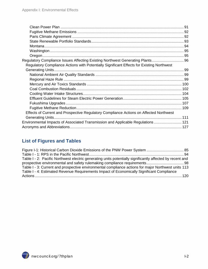
Appendix I: Environmental Effects
nwcouncil.org/7thplan I-2
Clean Power Plan .................................................................................................................... 91 Fugitive Methane Emissions .................................................................................................... 92 Paris Climate Agreement ......................................................................................................... 92 State Renewable Portfolio Standards ....................................................................................... 93 Montana ................................................................................................................................... 94 Washington .............................................................................................................................. 95 Oregon ..................................................................................................................................... 95
Regulatory Compliance Issues Affecting Existing Northwest Generating Plants .............................. 96 Regulatory Compliance Actions with Potentially Significant Effects for Existing Northwest Generating Units .......................................................................................................................... 99
National Ambient Air Quality Standards ................................................................................... 99 Regional Haze Rule ................................................................................................................. 99 Mercury and Air Toxics Standards ......................................................................................... 100 Coal Combustion Residuals ................................................................................................... 102 Cooling Water Intake Structures ............................................................................................. 104 Effluent Guidelines for Steam Electric Power Generation ....................................................... 105 Fukushima Upgrades ............................................................................................................. 107 Fugitive Methane Reduction ................................................................................................... 109
Effects of Current and Prospective Regulatory Compliance Actions on Affected Northwest Generating Units ........................................................................................................................ 111
Environmental Impacts of Associated Transmission and Applicable Regulations .......................... 121 Acronyms and Abbreviations ......................................................................................................... 127 List of Figures and Tables Figure I-1: Historical Carbon Dioxide Emissions of the PNW Power System ................................... 85 Table I - 1: RPS in the Pacific Northwest ......................................................................................... 94 Table I - 2: Pacific Northwest electric generating units potentially significantly affected by recent and prospective environmental and safety rulemaking compliance requirements ................................... 98 Table I - 3: Current and prospective environmental compliance actions for major Northwest units 113 Table I - 4: Estimated Revenue Requirements Impact of Economically Significant Compliance Actions .......................................................................................................................................... 120

Appendix I: Environmental Effects
nwcouncil.org/7thplan I-3
INTRODUCTION Appendix I describes effects on the environment from the main resources, both generation and conservation, in the Pacific Northwest that are either part of the existing power system or are likely candidates for the Seventh Power Plan’s new resource strategy. The appendix also discusses regulations that exist to address these environmental effects. The appendix begins with an overview of the broadly applicable major federal environmental regulations, before providing a narrative analysis of the associated effects of the region’s generating resources and the specific regulations that relate to those effects. The information in this appendix is background to inform the Council’s efforts to determine and quantify where possible the environmental costs and benefits of generating resources and, more broadly, give due consideration to environmental quality and the protection and mitigation of fish and wildlife as the Council develops the plan’s resource strategy. See Chapter 19 for a discussion of the Northwest Power Act’s requirements in this regard and how the Council is complying with the Act in developing the Seventh Power Plan. See Chapters 3, 9, 13, 15, and 20 for specifics on conservation and generating resources and on the way in which environmental information, including compliance costs, informed the analysis of resources and the selection of the resource strategy.
SELECTED MAJOR FEDERAL ENVIRONMENTAL LAWS AND REGULATIONS Several federal laws and regulations apply broadly to the lifecycle impacts of a variety of electricity generating resources. This section provides a brief primer on some of the federal laws that arise frequently in discussing the environmental effects of electricity production. In some instances, multiple environmental laws or regulations apply to a single pollutant, waste stream or activity, in these cases, the most stringent requirements generally control. To the extent that other federal, state, or local laws or regulations impose specific requirements or restrictions on a particular generating resource and are not addressed in this section, they will be discussed in the section describing the impacts of that resource.
National Environmental Policy Act The National Energy Policy Act of 1969 (NEPA) requires federal agencies conducting “major federal actions significantly affecting the quality of the human environment” to prepare a statement of the environmental impact of the proposed action and consider alternatives.1 Major federal actions are defined broadly to include official federal policies, plans, programs or permits.2 Subject to the discretion of each federal agency, certain actions are categorically excluded from the NEPA
1 https://www.law.cornell.edu/uscode/text/42/4332 2 Id.
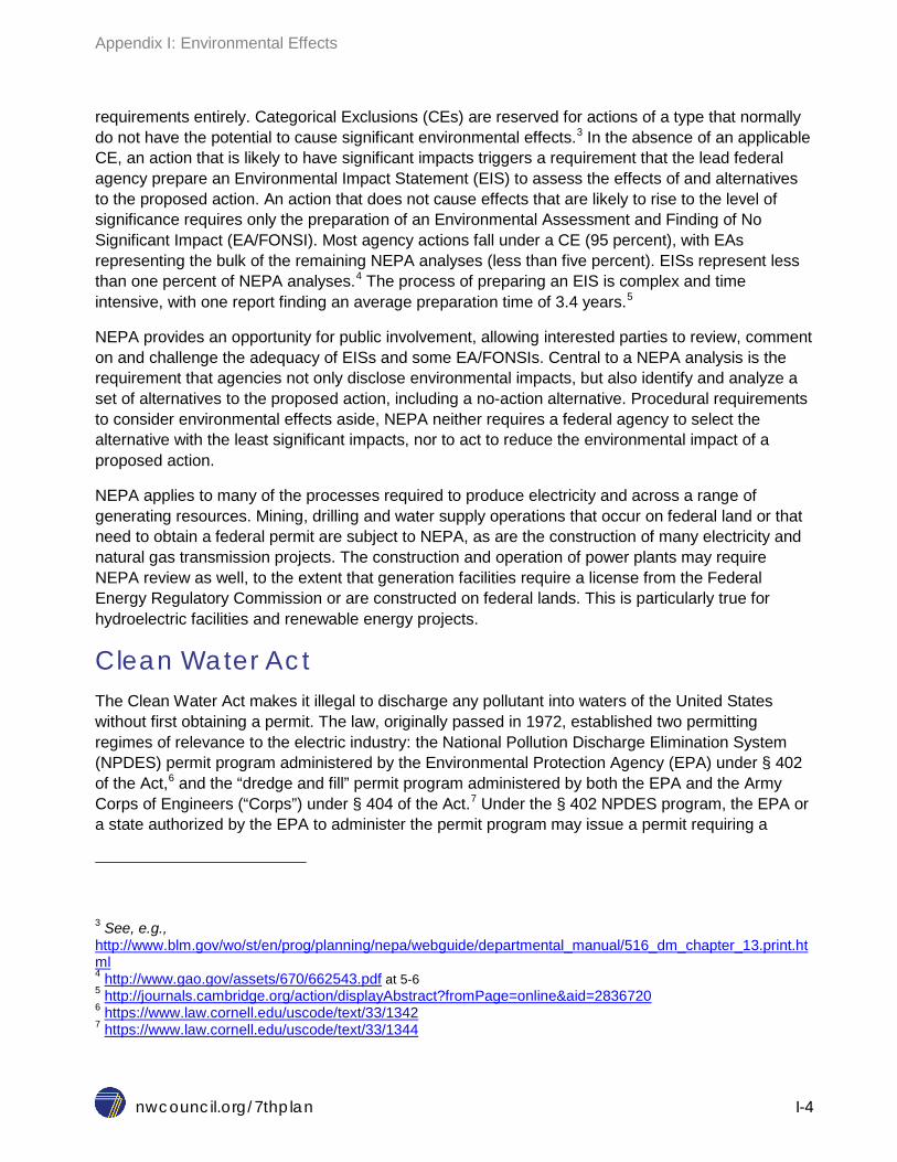
Appendix I: Environmental Effects
nwcouncil.org/7thplan I-4
requirements entirely. Categorical Exclusions (CEs) are reserved for actions of a type that normally do not have the potential to cause significant environmental effects.3 In the absence of an applicable CE, an action that is likely to have significant impacts triggers a requirement that the lead federal agency prepare an Environmental Impact Statement (EIS) to assess the effects of and alternatives to the proposed action. An action that does not cause effects that are likely to rise to the level of significance requires only the preparation of an Environmental Assessment and Finding of No Significant Impact (EA/FONSI). Most agency actions fall under a CE (95 percent), with EAs representing the bulk of the remaining NEPA analyses (less than five percent). EISs represent less than one percent of NEPA analyses.4 The process of preparing an EIS is complex and time intensive, with one report finding an average preparation time of 3.4 years.5
NEPA provides an opportunity for public involvement, allowing interested parties to review, comment on and challenge the adequacy of EISs and some EA/FONSIs. Central to a NEPA analysis is the requirement that agencies not only disclose environmental impacts, but also identify and analyze a set of alternatives to the proposed action, including a no-action alternative. Procedural requirements to consider environmental effects aside, NEPA neither requires a federal agency to select the alternative with the least significant impacts, nor to act to reduce the environmental impact of a proposed action.
NEPA applies to many of the processes required to produce electricity and across a range of generating resources. Mining, drilling and water supply operations that occur on federal land or that need to obtain a federal permit are subject to NEPA, as are the construction of many electricity and natural gas transmission projects. The construction and operation of power plants may require NEPA review as well, to the extent that generation facilities require a license from the Federal Energy Regulatory Commission or are constructed on federal lands. This is particularly true for hydroelectric facilities and renewable energy projects.
Clean Water Act The Clean Water Act makes it illegal to discharge any pollutant into waters of the United States without first obtaining a permit. The law, originally passed in 1972, established two permitting regimes of relevance to the electric industry: the National Pollution Discharge Elimination System (NPDES) permit program administered by the Environmental Protection Agency (EPA) under § 402 of the Act,6 and the “dredge and fill” permit program administered by both the EPA and the Army Corps of Engineers (“Corps”) under § 404 of the Act.7 Under the § 402 NPDES program, the EPA or a state authorized by the EPA to administer the permit program may issue a permit requiring a
3 See, e.g., http://www.blm.gov/wo/st/en/prog/planning/nepa/webguide/departmental_manual/516_dm_chapter_13.print.html 4 http://www.gao.gov/assets/670/662543.pdf at 5-6 5 http://journals.cambridge.org/action/displayAbstract?fromPage=online&aid=2836720 6 https://www.law.cornell.edu/uscode/text/33/1342 7 https://www.law.cornell.edu/uscode/text/33/1344
Appendix I: Environmental Effects
nwcouncil.org/7thplan I-5
discharger to comply with technology-based effluent limitations for various pollutants.8 The Act only requires a § 402 NPDES permit for discharges from a “point source,” which is defined as “any discernible, confined and discrete conveyance, including but not limited to any pipe, ditch, channel, tunnel, conduit, well, discrete fissure, container, rolling stock, concentrated animal feeding operation, or vessel or other floating craft, from which pollutants are or may be discharged.”9 When the EPA authorizes a state to administer the § 402 NPDES permitting program, the state will assume the responsibility to set effluent limitations guidelines and permit standards with which permittees must comply. The EPA administers the § 402 NPDES permitting program in states that have not been authorized. The EPA has partially or completely authorized Oregon, Washington and Montana; Idaho’s § 402 NPDES permit program remains federally administered.10 Nonpoint source pollution is not covered by the permit requirement and is typically regulated under state programs for the management of runoff. The cumulative effects of permitted point source discharges and nonpoint source runoff has resulted in impairment in a number of the nation’s waters.11
Under the § 404 dredge and fill permit program, the Corps (with the environmental guidance of the EPA) may issue a permit for the disposal of dredged or fill material within wetlands or waters of the United States.12 States may also assume authority to administer the § 404 dredge and fill permit program, however only two, Michigan and New Jersey, have done so to date.13
EPA or a state authorized to implement the Clean Water Act program in that state also set water quality standards for dozens or even hundreds of pollutants under § 303 of the Clean Water Act, standards which the point source, non-point source and dredge and fill programs together aim to satisfy. Water bodies that are not in compliance with one or more standards are subject to additional requirements under the Act or reduce the pollutant load.
Provisions in the Clean Water Act regulate the water impacts of a variety of lifecycle stages of electricity generation, including the mining and extraction of fuel, the construction of generation facilities and associated infrastructure, and the operation of hydroelectric and steam electric power plants.
Clean Air Act The modern Clean Air Act evolved from the Air Pollution Control Act of 1955. Under the current incarnation of the law, the EPA is responsible for establishing air quality standards and states are primarily responsible for ensuring compliance.14 The EPA currently administers three programs of primary relevance to the electricity sector: National Ambient Air Quality Standards (NAAQS),
8 http://www.in.gov/idem/files/rules_erb_20130213_cwa_summary.pdf at 5 9 http://water.epa.gov/lawsregs/guidance/wetlands/sec502.cfm 10 http://water.epa.gov/polwaste/npdes/basics/upload/State_NPDES_Prog_Auth.pdf 11 See http://iaspub.epa.gov/waters10/attains_nation_cy.control?p_report_type=T 12 http://www.in.gov/idem/files/rules_erb_20130213_cwa_summary.pdf at 6 13 http://water.epa.gov/type/wetlands/outreach/fact23.cfm 14 http://fpc.state.gov/documents/organization/155015.pdf

Appendix I: Environmental Effects
nwcouncil.org/7thplan I-6
National Emissions Standards for Hazardous Air Pollutants (NESHAPs), and New Source Performance Standards (NSPS).
Under § 109 of the Act, the EPA sets the NAAQS limiting the emission of air pollutants with the potential to endanger human health.15 Pursuant to this requirement, the EPA has identified six “criteria” pollutants for regulation under the NAAQS, including sulfur dioxide, particulate matter, nitrogen dioxide, carbon monoxide, ozone and lead.16 Once EPA sets the NAAQS, each state is responsible for developing the procedures necessary for compliance in its State Implementation Plan (SIP). The SIPs are subject to EPA approval. New and modified sources in a state must typically obtain permits that demonstrate compliance with allowable emissions limits. A region that exceeds the NAAQS for a specific pollutant is deemed a “nonattainment area,” and sources within that area must meet a special compliance schedule. Compliance requirements in nonattainment areas vary depending on the level of exceedance.
In addition to the NAAQS program, the Clean Air Act established a framework to limit hazardous air pollutant emissions. Under § 112 of the Act, the EPA establishes National Emissions Standards for Hazardous Air Pollutants (NESHAPs) for 187 listed air toxics: first, the EPA sets technology-based Maximum Achievable Control Technology (MACT) standards that represent “maximum degree of reduction in emissions…achievable” for each pollutant, taking cost into consideration; and second, to the extent that any residual health risks remain after the implementation of MACT, the EPA sets standards to “provide an ample margin of safety to protect public health…unless the Administrator [of the EPA] determines that a more stringent standard is necessary to prevent…an adverse environmental effect.” 17
The Clean Air Act, in § 111, also calls for the EPA to establish technology-based New Source Performance Standards (NSPS) that apply to categories of new industrial facilities.18 These standards set emissions limits for new major stationary sources based on the best adequately demonstrated control technology, considering cost.19 The NSPS is applied to existing facilities pursuant to the New Source Review program to the extent that the facilities undergo modifications.20 The recently finalized Clean Power Plan, which restricts carbon dioxide emissions, was promulgated under the NSPS program, §§ 111(b) and (d) of the Clean Air Act.21
These three programs, NAAQS, NESHAPs, and NSPS, frequently impose restrictions on emissions from an array of fossil-, nuclear- and biomass-fueled electricity generating technologies. Provisions of the Clean Air Act may also have implications for fuel extraction and transportation processes.
15 https://www.law.cornell.edu/uscode/text/42/7409 16 http://www3.epa.gov/airquality/urbanair/ 17 https://www.law.cornell.edu/uscode/text/42/7412 18 https://www.law.cornell.edu/uscode/text/42/7411 19 http://fpc.state.gov/documents/organization/155015.pdf at 12 20 Id. 21 See http://www2.epa.gov/cleanpowerplan

Appendix I: Environmental Effects
nwcouncil.org/7thplan I-7
Endangered Species Act Congress passed the Endangered Species Act (ESA) in 1973 with a purpose of protecting species threatened with extinction. Under the ESA, the U.S. Fish and Wildlife Service (FWS) in the Department of Interior and the fisheries agency of the National Oceanic and Atmospheric Administration in the Department of Commerce (NOAA Fisheries) are authorized to designate two classes of protected species: “endangered” species, which are those in danger of becoming extinct; and “threatened species,” which are those likely to become endangered.22 These listed species are protected against “take”, which is defined broadly to include “to harass, harm…wound, kill…or attempt to engage in any such conduct.”23 The take prohibition applies to “any person subject to the jurisdiction of the United States.”24 To effect the intended protections, the ESA also requires the designation of habitat critical to the conservation of the affected species. NOAA Fisheries has responsibility for anadromous fish and marine mammals, while the FWS’s purview extends to resident fish, wildlife, and plants.
Under § 7 of the ESA, no federal agency may authorize any action likely to jeopardize the survival of any listed species or harm their critical habitat.25 For that reason, a federal agency is required to consult with FWS or NOAA Fisheries prior to undertaking any action that may affect a listed species or critical habitat; to the extent that a proposed action is likely to adversely affect a listed species, the lead agency must seek a biological opinion from the FWS or NOAA Fisheries. The FWS and NOAA Fisheries may authorize an agency to act in a manner that results in “incidental take” of a listed species, consistent with reasonable and prudent measures to minimize the take.26
Under § 9, no person, including private citizens, may take a listed species or harm critical habitat.27 However, § 10 allows the FWS or NOAA Fisheries to permit take that is “incidental to… the carrying out of an otherwise lawful activity.”28 To obtain an incidental take permit, a person seeking the permit is required to prepare a habitat conservation plan that specifies the likely impact of the taking, the steps taken to minimize that impact, and the alternatives considered.29
The ESA impacts most types of electricity generating resources at various lifecycle stages. The best solar and wind resources often overlap with the habitat of sensitive species, implicating the ESA and causing tension between renewable energy and wildlife interests. Species and habitat may also be affected to the extent that forests are logged to provide timber or agricultural land for biomass feedstock production. With regards to fossil fuel-fired and nuclear generation, the mining and
22 https://www.law.cornell.edu/uscode/text/16/1532 23 Id. 24 https://www.law.cornell.edu/uscode/text/16/1538 25 https://www.law.cornell.edu/uscode/text/16/1536 26 See http://www.fws.gov/midwest/endangered/section7/section7.html 27 https://www.law.cornell.edu/uscode/text/16/1538 28 https://www.law.cornell.edu/uscode/text/16/1539 29 Id.

Appendix I: Environmental Effects
nwcouncil.org/7thplan I-8
extraction processes may occur in areas that implicate the ESA. Finally, linear infrastructure projects such as gas pipelines and electricity transmission lines may result in adverse habitat impacts.
ENVIRONMENTAL IMPACTS OF ELECTRICITY GENERATION AND APPLICABLE REGULATIONS BY RESOURCE TYPE The lifecycle impacts associated with electricity generation vary widely depending on the type, technology, fuel, size and location of the resources used. The varying processes involved in producing electricity mean that the profile of environmental and human health effects for each generating resource tends to be unique. The following sections discuss lifecycle impacts of each of the major generating resource types currently operating in the Pacific Northwest or identified in the new resource planning analysis as well as the legal and regulatory framework in place to address them.
Hydroelectricity Generation The Northwest relies significantly on hydroelectric generation to meet electricity demand in the region, with 31 federally-owned dams30 supplying over 40 percent of the region’s electricity.31 The Bonneville Power Administration markets the electricity produced by these dams, which together comprise the Federal Columbia River Power System (FCRPS).32 Other public and privately owned dams also contribute to the region’s electricity supply; all told, more than 200 hydroelectric facilities33 generate over half of the region’s power annually.
The principal environmental effects regarding hydroelectric development are generally focused on water quality impacts, hydrology impacts, erosion and sedimentation, land-use impacts, dust and noise during construction, and fish and wildlife impacts. The environmental effects associated with any one hydroelectric project are site specific and therefore can be very different when comparing projects; for example, a project that involves an existing dam or other existing water control structure will typically cause less of an incremental environmental impact than a project that requires new dam construction. There are few serious air emissions or solid waste issues associated with hydroelectric development or operation.
The construction and operation of a hydroelectric project may affect water quality through thermal changes (causing wide fluctuation of stream temperatures), nitrogen supersaturation (total dissolved gas), turbidity, and oxygen depletion. A hydroelectric dam slows the movement of water in a river
30 https://www.bpa.gov/power/pgf/hydrpnw.shtml#introduction 31 https://www.nwcouncil.org/history/Hydropower. The Northwest hosts over 200 hydroelectric facilities that generate around 70 percent of the region’s power. 32 https://www.bpa.gov/power/pgf/hydrpnw.shtml#introduction 33 See http://www.eia.gov/state/maps.cfm

Appendix I: Environmental Effects
nwcouncil.org/7thplan I-9
system, which can lead to temperature stratification and oxygen depletion in the reservoir behind the dam. Spill flows from a dam may increase the levels of total dissolved gas in the river downstream. While these water quality changes are not always adverse, they can have an effect on the aquatic environment and can prove lethal for fish and wildlife. Water quality can also affect the aesthetics of the project site.
The process of developing a hydroelectric dam alters the physical hydrology—the movement and distribution of water—of the site and the watercourse. These changes can have significant primary and secondary effects on water quality, habitat, and fish and wildlife. The operation of a hydroelectric facility during times of maintenance, outages, or to meet peak energy demands causes fluctuations of water level in both the impoundment and the stream below. These fluctuating water levels may prohibit development of shoreline vegetation, reduce shoreline use by riparian (riverbank or streamside) species of wildlife, and lower reproductive success of fish species that spawn near the impoundment margin. Fluctuations in rivers below dams can strand immature fish on shorelines or in shallow waters and may lead to the exposure of eggs of shoreline spawners and nests of salmonids. Storage dams tend to reduce some of the seasonal fluctuations in river flow, creating a more stable riparian zone and changes in habitat characteristics associated with variable flows. Impounded waters can flood islands that are important breeding grounds for certain avian species.
Issues with erosion and sedimentation may occur during construction and continue long after a project is retired or removed. Changes in the sediment load and flow can affect the natural sediment equilibrium found in free flowing waters and increase water turbidity due to accretion and settling in the backwaters behind a dam. This can result in increased sediment deposits near the physical dam and decreased sediment downstream, both affecting the growth of organisms that depend on nutrients carried by the sediment. As the water levels fluctuate, erosion can occur, changing the physical environment. A lack of vegetation along the riverbank can also lead to perpetual carving away of the earth surrounding the water source.
The amount of land required for the development of a hydroelectric dam varies significantly depending on the site and project. A storage project can take up thousands of acres, while a small run-of-river project may take up less than an acre. Nonetheless, between the physical infrastructure and the equipment used for construction, land is disturbed and the surrounding environment is altered.
During construction of a hydroelectric dam, significant amounts of dust, noise, and adverse aesthetics can negatively affect the surrounding project site. Dust and equipment noise is typically limited to the construction phase, whereas the aesthetics of the site are permanently altered. Hydroelectric plant operations are relatively quiet.
Of particular concern to the Council is the potential impact of hydroelectric development on fish and wildlife. While all of the above-mentioned environmental effects can directly or indirectly impact fish and wildlife, there are specific effects that are worth mentioning. A hydroelectric dam presents a migration barrier to the passage of upstream (adult) and downstream (juvenile) anadromous and resident fish. Habitat is completely blocked by some projects in the system. At dams that allow passage, juvenile downstream migrants face the risk of mortality at each dam as a result of passage through turbines, exposure to water supersaturated with nitrogen, delay in start of migration, increased travel times, and increased predation. Filling an impoundment behind a hydroelectric dam

Appendix I: Environmental Effects
nwcouncil.org/7thplan I-10
inundates land and transforms a free-flowing river into a lake-like environment. This transition of habitat changes the composition of terrestrial and aquatic biota at the project site which may be beneficial or detrimental to wildlife. System storage operations to optimize power generation also alter flows important for the emergence, rearing, and migration of juvenile salmon and other fish, and for adult spawning.
Under the Northwest Power Act, the Council develops a program to protect, mitigate, and enhance fish and wildlife adversely affected by the development and operation of hydroelectric facilities on the Columbia and its tributaries. To address the effects from the existing system, the Council’s Columbia River Basin Fish and Wildlife Program includes measures and objectives both to protect and increase survival of fish and wildlife within the hydroelectric system and to provide compensating offsite protection and mitigation. Measures to limit the direct impact of hydroelectric development include fish screens and bypass systems, bypass spills, and fish ladders to help fish navigate through the hydroelectric dam; minimum flows, flow augmentation requirements and stable storage reservoir operations; and the installation and implementation of systems to maintain powerhouse discharge and minimize or eliminate fluctuations in water and flow levels. Offsite protection and mitigation actions include both habitat protection and improvement measures and artificial propagation facilities and strategies. Mitigation for the effects of the development of the system on wildlife has focused primarily on the offsite acquisition, improvement and protection of habitat for the affected wildlife species.
The Council develops the Fish and Wildlife Program largely on the basis of recommendations from the federal and state fish and wildlife agencies and the region’s Indian tribes. The Bonneville Power Administration has an obligation under the Act to use its fund and authorities to protect, mitigate and enhance fish and wildlife in a manner consistent with the Council’s Fish and Wildlife Program. All the federal agencies that manage, operate or regulate the hydroelectric facilities (Corps of Engineers, Bureau of Reclamation, and Federal Energy Regulatory Commission, as well as Bonneville) have a separate obligation under the Act to exercise their statutory responsibilities to adequately protect, mitigate and enhance fish and wildlife in a manner that provides “equitable treatment” for fish and wildlife with the other project purposes and to do so taking into account the Council’s regional Fish and Wildlife Program at each stage of decision-making to the fullest extent practicable.
To provide guidance for future hydropower development in the region, the Council has designated approximately 44,000 miles of stream reaches as “protected areas,” where hydropower development would not be appropriate because of the damage development and operation would cause to fish, wildlife, and habitat. The protected areas designations are intended to protect fish and wildlife resources,34 send a clear signal to developers regarding the acceptability of stream reaches for hydroelectric development, provide power planning guidelines for determining the availability of new hydroelectric power, and create a comprehensive plan to provide guidance for licensing decisions made by the Federal Energy Regulatory Commission (FERC). As noted in the Council’s 2014
34 Protected areas designations are based on fish and wildlife considerations only and do not reflect other river values that might affect the desirability of hydroelectric development.

Appendix I: Environmental Effects
nwcouncil.org/7thplan I-11
hydropower scoping study,35 if a prospective site is located outside a protected area, it is not automatically deemed environmentally acceptable for hydroelectric development; each project must undergo extensive environmental impact studies approved by state and federal agencies in order to proceed.
Detail on both the effects of hydroelectric production and the protection and mitigation measures to address those effects can be found in the past and current Fish and Wildlife Programs. The Council adopted its latest amendments to the Columbia River Basin Fish and Wildlife Program in October 2014.36 The 2014 Fish and Wildlife Program is part of the draft Seventh Power Plan. See Chapter 20, as well as the discussion in Chapter 19. A number of species affected by the hydroelectric system are also listed as threatened or endangered under the federal Endangered Species Act, including 13 distinct population segments of salmon and steelhead, Kootenai River white sturgeon, bull trout, and eulachon. The Fish and Wildlife Program includes a discussion of and links to the programs, plans, biological opinions, and other developments related to addressing the requirements of the ESA for these species, as well as a discussion as to how the ESA requirements and programs interrelate with the regional protection and mitigation program under the Northwest Power Act. The licensed issues by FERC under the Federal Power Act to the owners and operators of the non-federal hydroelectric dams on the Columbia and its tributaries include fish and wildlife protection and mitigation requirements to address the requirements of the Federal Power Act, the Northwest Power Act, and ESA.
For details on the environmental effects of hydroelectric pumped storage, see the “Electricity Storage” section below.
Coal-Fired Electricity Generation Although coal-fired power plants still produce more electricity in the US than any other resource type, coal use in the electricity sector is declining.37 The Energy Information Administration (EIA) forecasts that coal-fired generators will produce 28 percent less electricity in 2015 than they did during coal’s recent peak in 2007, a decline attributable in part to low natural gas prices and the growth of renewable energy.38 In addition to these competitive pressures, the Environmental Protection Agency’s Clean Power Plan will potentially limit coal-fired electricity generation in the future by establishing a carbon dioxide emissions reduction target of 32 percent less carbon dioxide (CO2) from the electric industry by 2030, based on 2005 emissions levels.39 Coal, as the most significant contributor to carbon dioxide emissions in the electric industry, stands to see the biggest impact from the EPA’s Clean Power Plan regulations.
35 http://www.nwcouncil.org/energy/grac/hydro/ 36 http://www.nwcouncil.org/fw/program/2014-12/program/ 37 http://www.eia.gov/forecasts/steo/images/Fig25.png 38 http://www.eia.gov/forecasts/steo/report/coal.cfm 39 http://www2.epa.gov/cleanpowerplan/fact-sheet-clean-power-plan-numbers

Appendix I: Environmental Effects
nwcouncil.org/7thplan I-12
However, advancements in carbon capture and sequestration (CCS) technologies may present coal with a renewed opportunity for growth in the future. The CCS process involves removing carbon dioxide from a plant’s emissions and transporting it to a facility where it can be injected into deep geological formations.40 Despite the promise of reduced CO2 emissions, CCS technologies are currently too costly for widespread deployment. Including CCS technologies in the construction of a new coal plant raises the levelized cost of electricity produced by that facility by approximately 44 percent to 80 percent (depending on the type of plant), and retrofitting an existing facility is still more costly.41 Absent a significant reduction in the cost of CCS, the electric industry’s reliance on coal as a generation resource is likely to its decline. The national trend towards coal plant retirements is mirrored in the Northwest, where four of the six coal-fired power plants providing electricity to the region are slated to close in the next 10 years, and regional policymakers are considering legislation to facilitate the closure of the other two.42 Still, because coal-fired electricity generation is expected to continue to provide power to the Northwest in the near term, and advances in CCS technologies may make coal an attractive fuel in the future, it is important to consider the environmental consequences of these plants.
While carbon dioxide emissions from coal plants represent the issue of most concern at present, the lifecycle environmental and human effects of coal-fired electricity generation are many and varied. The following sections examine the impacts associated with coal mining, processing, and transportation as well as the effects of coal plant construction and operations.
Impacts of Coal Mining, Processing, and Transportation
Coal is a sedimentary rock composed of organic matter that has been subjected to geologic heat and pressure over millions of years, a process that forms underground seams of the fuel that may be extracted either through surface or underground mining operations. Coal is typically processed at the mine site to remove impurities before transportation to a power plant. Once coal has been prepared, it is generally shipped to a power plant by train, barge or truck or pipeline.43 Each of these stages, coal mining, processing and transportation may cause adverse environmental and human health effects.
Coal is extracted either from underground mines, which account for approximately one-third of the coal produced in the US, or surface mines, which produce about two-thirds of the domestic supply.44 Underground mines have limited surface impacts, relying on discreet above-ground points of entry to enable miners and equipment to access the coal seam. The development of an underground mine typically involves the transportation of heavy equipment and workers to the site, which may require the construction of new roads. In addition, preparation of the site may entail drilling, blasting, excavation and pile driving. These operations often result in air impacts from fugitive dust and
40 http://www.epa.gov/climatechange/ccs/ 41 http://www.c2es.org/technology/factsheet/CCS 42 http://www.nytimes.com/2015/02/15/us/politics/bills-in-washington-state-seek-to-end-use-of-coal.html?_r=0 43 http://www.epa.gov/cleanenergy/energy-and-you/affect/coal.html 44 http://www.eia.gov/coal/annual/pdf/acr.pdf

Appendix I: Environmental Effects
nwcouncil.org/7thplan I-13
vehicle exhaust, as well as water impacts from altered drainage patterns and increased pollutant and sediment loads in runoff from the site. Wildlife may be affected by associated noise and human activity, as well as habitat disruption.
Underground coal mining is typically conducted by one of two methods: room-and-pillar mining, in which the miners excavate portions of the coal seam but leave pillars of coal to support the ground above, or longwall mining, in which a mechanical shearer and hydraulic roof supports are used to mine a long panel of coal in a series of slices, allowing the mined area to collapse a safe distance behind the miners and equipment. Longwall mining recovers more of the available coal than room-and-pillar operations and is generally the most cost-effective method of underground mining.45 Subsidence of the land surface above a mine is a significant concern for both methods of underground mining, potentially damaging buildings, utility and transportation infrastructure, surface and groundwater resources, vegetation, and wildlife habitat.46 A longwall mine is more likely to cause subsidence, because the mined area is intentionally permitted to collapse behind the shearing operation. The subsidence impacts of a longwall mine are generally more uniform and contemporaneous than subsidence resulting from a room-and-pillar mine, and are therefore easier to forecast and mitigate. Subsidence as a result of underground mining is regulated federally under the Surface Mining Control and Reclamation Act (SMCRA), which requires mine operators to adopt measures to prevent subsidence that causes material damage.47 The Office of Surface Mining, Reclamation and Enforcement (OSMRE) issues permits for underground mines, requiring the permittee to prevent subsidence to the extent feasible, and repair or compensate for damage caused as a result of subsidence.48 The law and associated regulations allow for planned subsidence in a predictable and controlled manner.
Underground mines also pose greater risks to mineworkers than their surface counterparts. Pulmonary diseases, including coal workers’ pneumoconiosis, silicosis, and chronic obstructive pulmonary disease, are a significant concern for underground mineworkers who work in a confined area with high levels of coal dust and silica in the air.49 Underground mineworkers are additionally faced with greater risks associated with mining accidents such as unintended collapses50 and explosions.51 Underground coal mining processes release methane contained within coal seams; methane is extremely flammable, toxic to humans and a greenhouse gas that contributes to climate change to the extent it is not captured.52 Mineworker protection is regulated primarily by the Mine Safety and Health Administration (MSHA) under the Federal Mine Safety and Health Act of 1977, as
45 http://www.bloomberg.com/news/articles/2015-08-10/the-30-year-old-trick-that-s-going-to-keep-america-s-coal-alive 46 http://pubs.usgs.gov/circ/1983/0876/report.pdf 47 https://www.law.cornell.edu/uscode/text/30/1266 48 https://www.law.cornell.edu/cfr/text/30/817.121 49 http://www.cdc.gov/niosh/docs/2011-172/pdfs/2011-172.pdf 50 http://www.post-gazette.com/local/region/2015/03/08/Roof-Collapse-at-Cameron-Mine-Portal-Possible-Entrapment/stories/201503080217 51 http://www.nytimes.com/2010/04/10/us/10westvirginia.html?pagewanted=all 52 http://www.epa.gov/cmop/faq.html

Appendix I: Environmental Effects
nwcouncil.org/7thplan I-14
amended in 2006.53 This law gives the MSHA the authority to promulgate safety standards, inspect mines, and investigate accidents.54 In addition, the Department of Labor operates a program under the Black Lung Benefits Act to compensate miners and survivors of miners who suffer from or are killed by pneumoconiosis.55
While an underground mine causes surface impacts generally limited to the access points of the mine, a surface coal mine causes significantly more visible above-ground impacts. The two predominant methods of surface coal mining are mountaintop removal, which commonly occurs in the Appalachian coalfields, and area strip mining, which is typically employed in the Western states. Mountaintop removal mining involves the use of explosives and machinery to access coal seams beneath mountaintops.56 The displaced rock and dirt, called “overburden,” is disposed of in adjacent valleys. In addition to causing harmful effluents, mountaintop removal operations often permanently bury headwater streams with overburden and alter flow patterns in associated drainages.57 Once mining operations are complete, the area is regraded and revegetated.58 A 2002 revision of the Army Corps of Engineers’ regulations revised the definition of fill material to include “overburden, slurry, or tailings or similar mining-related materials,” making explicit the ability of mountaintop removal mining operations to continue valley fill practices.59 These practices are limited to ½ an acre and 300 linear feet of stream bed loss under a general permit, but broader valley fill operations may be permitted under an individual permit. In addition to compliance with the Clean Water Act, valley fill operations require a regulatory exception from the OSMRE for surface mining activities that would disturb the land within 100 feet of a stream.60 The current regulatory regime allows for considerable potential residual environmental effects from valley fill practices. The OSMRE has recently proposed regulations to strengthen its stream protection program,61 but it does not appear likely that these proposed regulations would significantly alter valley fill practices.62 After mining operations are complete, mined areas must be reclaimed pursuant to requirements in the Surface Mining and Control Act. Surface mines must typically be restored to their “approximate original contour” under the Act, however, mountaintop removal mines are exempted so long as the land is left level or gently rolling.63 Even after reclamation, then, the character of areas subjected to mountaintop removal mining operations is significantly and permanently altered. In Appalachia, where mountaintop removal mines are frequently located in areas covered by deciduous forests that host significant
53 https://www.law.cornell.edu/uscode/text/30/811 54 https://www.law.cornell.edu/uscode/text/30/813 55 http://www.dol.gov/owcp/dcmwc/regs/compliance/blfact.htm 56 http://www3.epa.gov/region03/mtntop/ 57 Id. 58 Id. 59 https://www.fas.org/sgp/crs/misc/RL31411.pdf at 5. 60 http://www.gpo.gov/fdsys/pkg/CFR-2013-title30-vol3/pdf/CFR-2013-title30-vol3-sec816-57.pdf 61 http://www.osmre.gov/programs/RCM/docs/SPRProposedRule.pdf 62 Id. “…[N]othing in the proposed revisions to our excess spoil requirements would prohibit the construction of valley fills, head-of hollow fills, sidehill fills, or any type of fill other than durable rock fills.” 63 https://www.law.cornell.edu/cfr/text/30/824.11

Appendix I: Environmental Effects
nwcouncil.org/7thplan I-15
biodiversity,64 this permanent alteration of the land can represents a significant ongoing environmental impact.65
Area strip mining uses a similar process to mountaintop removal, in which heavy machinery is used to remove soil and rock in order to access underlying coal seams. Large scrapers remove the soils covering the area to be mined, and either stockpile the soils for later reclamation use or use them to reclaim a previously mined area.66 The overburden beneath the soils is then leveled, blasted and removed to a spoils pile to expose the underlying coal seam. These methods of surface mining have obvious implications for vegetation, which must be removed prior to mining operations, and wildlife habitat, which relies on the natural character of the land. The affected species and degree of impact depend on the type and location of mining operation. Western strip mines are often coterminous with the habits of sensitive wildlife, such as sage grouse and mule deer. Despite the potential wildlife impacts, surface coal mining operations are not required to conduct a § 7 consultation with the Fish and Wildlife Service (FWS) under the Endangered Species Act, even where there is federal involvement in the project. This arrangement is based on the FWS’s 1996 Biological Opinion on Surface Coal Mining and Reclamation, which reasoned that the environmental regulations under the Surface Mining Control and Reclamation Act were sufficiently protective of wildlife to find that mining activities would have no effect on listed species or critical habitat under the ESA.67
Surface mines may have a detrimental impact on water quality as well. Surface mining often results in acidic runoff containing harmful levels of sediment, salinity and trace metals.68 This runoff is generally nonpoint source pollution, as such it is not regulated by the EPA.69 Nonpoint source pollution is regulated by state management programs under the Clean Water Act, but the nonpoint waste stream is notoriously difficult to manage and these programs have yielded little improvement in water quality.70 Many aquatic organisms, including fish species are sensitive to minor water quality changes. Sulfate present in mine runoff, for example, results in microbial production of hydrogen sulfide, which is toxic to many aquatic organisms, and selenium bioaccumulation causes deformities in certain fish species and reproductive harm to the birds that eat them.71 Sediment adversely impacts salmonid spawning and rearing, and can reduce reservoir capacity and damage hydroelectric infrastructure. These impacts to aquatic organisms are regulated to some degree by SMCRA’s environmental performance protection standards, which require that mine operators “to the extent possible using the best technology currently available, minimize disturbances and adverse impacts of the operation on fish, wildlife, and related environmental values, and achieve enhancement of such resources where practicable.”72 The OSMRE has proposed regulations to strengthen the protections for fish and wildlife, including the restoration of native vegetation to mined
64 http://www.filonverde.org/images/Mountaintop_Mining_Consequences_Science1[1].pdf 65 http://www.scientificamerican.com/article/endangered-species-coal-appalachia-mountaintop-removal/ 66 http://www.epa.gov/ttnchie1/ap42/ch11/final/c11s09.pdf 67 http://www.fws.gov/ecological-services/es-library/pdfs/96_US_OSM.pdf 68 http://www.ncbi.nlm.nih.gov/pmc/articles/PMC3248525/ 69 https://www.law.cornell.edu/uscode/text/33/1329 70 http://www.gao.gov/assets/600/591303.pdf 71 http://www.filonverde.org/images/Mountaintop_Mining_Consequences_Science1[1].pdf 72 https://www.law.cornell.edu/uscode/text/30/1265#FN-2

Appendix I: Environmental Effects
nwcouncil.org/7thplan I-16
areas, enhanced water quality monitoring requirements, and improved handling of acid- and toxic-forming materials.73 The effect of these proposed regulations remain to be seen.
Air impacts associated with surface mining include the release of methane trapped within coal seams, vehicle exhaust from the use of heavy equipment, and overburden dust and coal dust aerosolized by blasting and wind erosion.74 Coal mines emitted over 140 billion cubic feet of methane in 2012, of which surface mines were responsible for 17 percent. EPA runs a voluntary program to capture and mitigate fugitive methane emissions from both underground and surface coal mines called the Coalbed Methane Outreach Program.75 The success of this program in reducing methane emissions is uncertain.
Surface mines, particularly mountaintop removal mines, are associated with a variety of human health impacts. In addition to significant noise levels, blasting causes vibrations that can compromise adjacent landowners’ buildings and wells.76 Dust and “flyrock” from blasting operations can travel beyond the property boundaries of the mine, settling on adjacent properties.77 Surface mines may degrade downstream water quality, potentially causing illness in people who come in contact with the water.78 The alteration of drainages through the practice of “valley fill” disposal of overburden increases the likelihood of flooding, impacting downstream residents.79 Microbes metabolize the sulfate present in mining runoff into hydrogen sulfide gas, inhalation of which, in addition to producing an unpleasant “rotten egg” smell, appears to cause headaches, irritability and memory loss.80 Ecological impairment of streams as a result of coal mining operations may increase cancer mortality for individuals living in the surrounding area.81 A 2010 study of West Virginia residents found a correlation between rising rates of breast, respiratory and urinary cancers and the degree of stream impairment from mining activities.82 In addition to direct human health impacts, surface mining may also result in a variety of indirect human health effects. Active surface mines occupy large areas of land and are incompatible with alternative land uses, so mining reduces recreational opportunities and causes considerable aesthetic impacts. Improper management of mine sites can lead to coal seam fires, which may smolder underground for decades.83 Coal seam fires burn underground, releasing toxic gases through surface vents and causing subsidence. The environmental and human health effects associated with mountaintop removal mining, both real and perceived, drive down property values in nearby communities and can result in the displacement of
73 https://www.law.cornell.edu/uscode/text/30/1265#FN-2 74 http://www.epa.gov/ttnchie1/ap42/ch11/final/c11s09.pdf 75 http://www3.epa.gov/cmop/basic.html 76 https://www.fas.org/sgp/crs/misc/RS21421.pdf at 4. 77 Id. 78 http://www.ncbi.nlm.nih.gov/pmc/articles/PMC3226519/ 79 Id. 80 Id. 81 http://www.ncbi.nlm.nih.gov/pmc/articles/PMC3226519/ 82 Id. 83 http://www.portal.state.pa.us/portal/server.pt/community/centralia_mine_fire_resources/21339

Appendix I: Environmental Effects
nwcouncil.org/7thplan I-17
residents and municipal infrastructure.84 Surface mining may also adversely impact significant cultural or paleontological sites, including town cemeteries.85 Under the OSMRE’s regulations pursuant to SMCRA, mine operators must catalogue cultural, historic and archeological resources prior to the commencement of mining activities.86 These resources may be protected to the extent that they are eligible for listing in the National Register of Historic Sites, but exceptions to the protections may be granted by a relevant regulatory authority.87 Communities located near surface mining operations may also encounter additional human health impacts from the processing and transportation of coal, discussed below.
Limited coal mining in the Northwest means that coal plants in the region import most of their fuel from Western coalfields or Appalachia. Wyoming is the largest coal producing state, accounting for 39 percent of US coal, followed by West Virginia at just over 11 percent.88 The largest surface coal mine in the US, Peabody Energy’s North Antelope Rochelle Mine, covers approximately 46,000 acres in Wright, Wyoming89 and generated over 110 million tons of coal in 2013.90 Montana is the only state in the Northwest that hosts significant coal mining operations, producing just over 4 percent of the country’s coal predominantly from the state’s surface mines.91 Most of the coal burned in the Northwest for electricity production is from the Powder River Basin in Wyoming and Montana.92
After coal is mined from either an underground or surface mine, it is typically processed to remove impurities before being transported to a coal plant. Coal arrives at a cleaning facility as run-of-mine coal, where it is stored in stockpiles until needed. From there, the coal is crushed and screened into fine and coarse fractions, which are subsequently conveyed to their respective cleaning processes.93 Processing methods for fine and coarse coal are similar; typically the coal is washed with water or other fluids to allow the lighter coal particles to separate from the denser impurities such as rock, soil, and ash. The moisture must then be removed from the coal through dewatering and thermal drying.94 Dewatering typically involves the use of screens, thickeners or cyclones to separate the water from the coal, while dewatered coal is thermally dried by exposure to hot gasses.95 Once it is dry, the coal is ready for combustion in a coal plant. Processing generally occurs at or near the mine site to reduce transportation costs of the fuel.
84 http://blogs.wvgazettemail.com/coaltattoo/2010/04/29/annenberg-foundation-offering-2-5-million-toward-new-marsh-fork-elementary-school/ 85 http://news.nationalgeographic.com/news/2013/09/130906-twilight-strip-mine-cemetery-west-virginia/ 86 http://www.ecfr.gov/cgi-bin/text-idx?SID=4efe39d682156fd82b3ec3ad615a8d9c&mc=true&node=se30.3.779_112&rgn=div8 87 https://www.law.cornell.edu/uscode/text/30/1272. See also http://www.ecfr.gov/cgi-bin/text-idx?SID=652b47adf00515bf291385ee478048b6&mc=true&node=se36.1.60_12&rgn=div8 88 Id. 89 http://www.osmre.gov/resources/reports/2012.pdf at 28. 90 http://www.peabodyenergy.com/content/274/publications/fact-sheets/north-antelope-rochelle-mine 91 Id. There is only one underground coal mine in operation in Montana. 92 http://www.eia.gov/coal/transportationrates/archive/2010/index.cfm 93 http://www.epa.gov/ttnchie1/ap42/ch11/final/c11s10.pdf 94 Id. 95 Id.

Appendix I: Environmental Effects
nwcouncil.org/7thplan I-18
The coal cleaning process raises a variety of environmental and human health concerns, primarily resulting from the water effluents associated with the cleaning process. Run-of-mine coal stockpiles may be stored outside, uncovered, which exposes them to wind and rain. Rainwater leaches contaminants from the coal, and the runoff is generally captured in a coal pile runoff pond.96 These contaminants include metals such as copper, aluminum, nickel, and iron, as well as suspended solids. Coal pile runoff ponds are designed to settle out solids, but typically do not treat the water for metal content before discharging.97 Effluents are also produced in the coal washing process, where much of the non-coal material removed during preparation of the coal is suspended in water and stored in tailings ponds. These ponds may contain billions of gallons of slurry, contaminated with coal particles, dirt, rock, clay and an array of metals and other pollutants.98 Unintentional release of the coal slurry through impoundment failure99 or an accident in transportation100 can lead to significant damage to downstream ecological resources, property and community health. Coal waste impoundments may require both a § 404 dredge and fill permit from the Corps—to the extent that the impoundment is constructed in a stream or wetland—and a § 402 NPDES permit from the EPA—to the extent that the impoundment discharges into a waterbody.101 Even absent unintentional release, the presence of a coal slurry impoundment may cause public anxiety about the potential for a breach or water contamination in nearby communities. This public perception reduces property values and drives relocation efforts.102 The chemicals used in coal washing may have adverse ecological and human health effects as well, to the extent that they are exposed to the environment through the washing process or accidental release from holding tanks.103 The extent of the impacts depends on the chemicals and amount involved, although the effects of many of these chemicals are little understood until an accident occurs.104
In addition to water effluents, coal processing may result in particulate matter air emissions in the form of coal dust during conveyor belt pour off, stockpile construction or consumption, crushing and sorting operations, thermal drying or through wind erosion.105 Coal dust may contribute to the health effects experienced by individuals living near mining operations.106 Particulate emissions can be mitigated through control technology or dust suppression measures, including water wetting.107 Fugitive dust from coal processing is regulated by the EPA under the New Source Performance Standards (NSPS) of the Clean Air Act (CAA). The standards apply to thermal dryers, pneumatic
96 http://water.epa.gov/scitech/wastetech/guide/304m/upload/2008_09_10_guide_304m_2008_steam-detailed-200809.pdf at 3-61. 97 Id at 3-62. 98 http://www.nytimes.com/2000/12/25/us/a-torrent-of-sludge-muddies-a-town-s-future.html 99 Id. 100 http://www.wvgazettemail.com/News/201402110032 101 http://water.epa.gov/polwaste/npdes/Mining.cfm 102 See, e.g. the Marsh Fork Elementary School relocation saga. http://www.wvgazettemail.com/News/201301200022. Also referenced in note 84. 103 http://www.newyorker.com/magazine/2014/04/07/chemical-valley 104 http://ntp.niehs.nih.gov/results/areas/wvspill/studies/index.html 105 http://www.epa.gov/ttnchie1/ap42/ch11/final/c11s10.pdf 106 See, e.g., http://www.scopemed.org/fulltextpdf.php?mno=20068 107 Id.

Appendix I: Environmental Effects
nwcouncil.org/7thplan I-19
coal cleaning equipment, coal processing and conveying equipment, and coal storage, transfer and loading systems that process more than 200 tons of coal per day.108 Numeric emissions standards are established for particulate matter and opacity, as well as sulfur dioxide, oxides of nitrogen and carbon monoxide emissions and are designed reflect the emissions levels achievable through the use of best demonstrated control technology.109 The regulations also require regular monitoring and reporting.110
After the coal has been processed to remove impurities, it is transported to a coal fired power plant by truck, rail, barge, or pipeline. Most of the coal received by power plants is shipped by rail (72 percent), followed by barge (11 percent), truck (10 percent) and conveyor or pipeline (7 percent).111 The primary impacts of coal transportation can include air emissions, water contamination, and noise and traffic levels.112 Coal transportation causes two primary air impacts: coal dust release and vehicle emissions. In addition to coal dust released during the loading and unloading of coal, the act of transportation itself may cause fugitive coal dust emissions. In a 2009 testimony before the Rail Energy Transportation Advisory Committee, a railroad company executive estimated that a single railcar may lose as much as 645 pounds of coal per 400 mile trip.113 A typical Northwest coal train may consists of five locomotives and up to 145 open-top hopper cars.114 Truck transport of coal causes similar issues on a smaller scale. In addition to the health impacts of coal dust discussed above, landowners adjacent to loading or unloading sites and transportation routes may experience a persistent coating of coal dust around and inside their homes.115 Water impacts from coal transportation can occur from fugitive emissions of coal dust and fuel system emissions during loading, unloading and transportation by barge.116 Coal pipelines allow pulverized coal that has been mixed with water to flow from a coal processing facility to a power plant. The coal must be dewatered and dried prior to use, resulting in spent water that is contaminated with many of the same materials present in coal processing effluents. The spent water may be used in the cooling system of a coal-fired power plant or recycled through a return pipeline.117 Additionally, individuals living near sites at which coal is loaded and unloaded as part of the transportation process may experience significant levels of noise, and truck or train traffic from the facility.
Both underground and surface coal mine sites are typically decommissioned and reclaimed to mitigate ongoing environmental impacts. Decommissioning and reclamation typically involves removing mining infrastructure, filling in the mine site and recontouring the land, and revegetating
108 http://www.ecfr.gov/cgi-bin/text-idx?SID=1665e9cf519d9554e8a83ce44386e7e2&mc=true&node=sp40.7.60.y&rgn=div6 109 http://www3.epa.gov/ttn/caaa/t1/fr_notices/cpp_nsps_fr_092509.pdf at 17. 110 http://www.ecfr.gov/cgi-bin/text-idx?SID=1665e9cf519d9554e8a83ce44386e7e2&mc=true&node=sp40.7.60.y&rgn=div6 111 http://www.eia.gov/coal/transportationrates/archive/2010/trend-coal.cfm#fig1 112 http://www.che.utexas.edu/course/che359&384/lecture_notes/topic_3/Chapter4.pdf 113 http://www.scribd.com/doc/129350651/Surface-TransMinutes-9-10-09-1 114 http://www.oregonlive.com/environment/index.ssf/2012/06/coal_clash_trains_roll_slowly.html 115 http://newstandardnews.net/content/index.cfm/items/3141 116 http://www.che.utexas.edu/course/che359&384/lecture_notes/topic_3/Chapter4.pdf 117 https://www.princeton.edu/~ota/disk3/1978/7817/781706.PDF
Appendix I: Environmental Effects
nwcouncil.org/7thplan I-20
the area.118 The impacts of the decommissioning and reclamation stage of a coal mining operation are primarily associated with the operation of construction equipment on the site.119 Residual impacts may persist after a mine site has been decommissioned and reclaimed. These impacts include: altered surface or groundwater flow patterns, breach or seepage of contaminated effluent from tailings ponds, and wildlife habitat and visual impacts resulting from topographical changes to the land.120
If a federal agency leases land or issues a permit for proposed coal mine operations or coal-fired electricity generating facilities, the NEPA may impose procedural requirements on the project. The NEPA requires federal agencies to conduct environmental analyses of proposed actions; the scope and complexity of the analyses depends on the application of CEs to the project in addition to the significance of the environmental effects. Preparation of a full EIS, which is required when a proposed action is likely to have significant impacts, involves a considerable investment of time and resources.
Impacts of Operating a Coal Power Plant
A coal-fired steam-electric power plant consists of coal receipt, storage, handling and preparation facilities, a furnace and steam generator, a steam turbine and condenser, an electric power generator, a switchyard, flue gas handling and emission control equipment and a closed-cycle condenser cooling system. In the Northwest, most plants use pulverized coal firing to achieve essentially complete combustion. All operate with subcritical steam pressure and temperature conditions, unlike the somewhat more efficient state-of-the-art supercritical or ultra-supercritical designs. All operational coal plants in the region use some form of closed-cycle cooling.121 These plants normally operate as baseload units, coming down only for maintenance and seasonal economic outages.
An array of environmental and human health impacts may result from the construction, operation and decommissioning stages of a coal power plant’s lifecycle. Although the construction of new coal-fired electricity generation facilities in the Northwest appears unlikely at this point in time, advancements in CCS technologies and fluctuations in fuel prices may spur coal plant development in the future. As such, an analysis of the environmental and human health impacts of the construction phase of a coal facility is important. The construction of a coal plant may result in soil erosion and associated water quality impacts during site preparation, increased air emissions related to the transportation of construction material and the operation of heavy equipment, wildlife disruption and loss of habitat, and nuisances to adjacent property owners, including increased vehicular traffic, noise and dust.122 The production of concrete, transportation of construction
118 http://teeic.indianaffairs.gov/er/coal/impact/decom/index.htm 119 Id. 120 http://teeic.indianaffairs.gov/er/coal/impact/decom/index.htm 121 The Corette plant in Billings, Montana, was the only Northwest coal plant that used once-through cooling, however, Corette was retired in August, 2015. 122 http://teeic.indianaffairs.gov/er/coal/impact/construct/index.htm

Appendix I: Environmental Effects
nwcouncil.org/7thplan I-21
materials, and operation of construction equipment all have the potential to cause air emissions.123 Although most of these impacts are temporary, the disruption of wildlife and loss of habitat, and nuisances to adjacent landowners may persist beyond the duration of the construction phase. Under the Clean Water Act, a developer is required to obtain a § 402 NPDES permit from the EPA or authorized state for stormwater discharges that occur during construction of a coal plant.124
The operation phase of coal-fired electricity generation has the potential to result in significant environmental and human health impacts, notably air emissions, impacts on water quality and quantity. Atmospheric releases of an assortment pollutants are the primary environmental impact of coal-fired plants. Pollutants of concern include particulates, sulfur oxides, nitrogen oxides, mercury and other heavy metals, and carbon dioxide.125 Direct particulate emissions from coal plants firing pulverized coal originate from incombustible constituents of coal. Most of the resulting ash settles to the bottom of the furnace and is removed for landfill or settling pond disposal, but some is entrained in the flue gas. Plants are provided with fabric filters (“baghouses”) or electrostatic precipitators to capture particulates in the flue gas. Some particulates are also captured in wet flue gas desulfurization (FGD) equipment. Particulate control technology capture efficiency ranges from 99 percent to 99.9 percent.
Particulate matter (PM) is airborne solid or liquid matter including dirt, dust, soot, smoke, and liquid droplets. Respirable particulates, or particles that capable of being inhaled, are classified as PM10 (less than 10 microns in diameter) and PM 2.5 (particles smaller than 2.5 microns). Particulates originate from incomplete fuel combustion and noncombustible fuel components. Secondary particulates originate from reactions of precursor compounds including nitrogen oxides or sulfur dioxide. In addition to the causes of particulate matter emissions discussed above (dust from mining, coal preparation, coal transportation, and open fuel storage), particulate matter is often a product of cooling tower drift and ash disposal operations.
Particulates can have adverse effects on health, materials, cleanliness and visibility. Respirable particles can lodge in the lungs, causing or aggravating diseases of the heart and lungs, decreased lung function, coughing, difficulty breathing and other pulmonary irritation. Fine particles are the major component of haze. Acidic derivatives of certain particulate species are a cause of acid rain, with adverse effects on surface waters, soils, and sensitive species. Acid rain and dry deposition of acidic particles can also degrade metals, stone, coatings and other materials. Particulate deposition dirties buildings and other structures causing aesthetic impacts and increasing maintenance costs. Black carbon, a form of PM 2.5 and a product of incomplete coal combustion, accelerates ice and snow melt through deposition by reducing its ability to reflect sunlight.126
123 Id. 124 http://yosemite.epa.gov/r10/water.nsf/npdes+permits/region+10+cgp+resources/ 125 Unless otherwise noted, the following discussion of air pollutants and controls associated with coal-fired electricity generation is derived from Environmental Protection Agency AP-42 Compilation of Air Pollutant Emission Factors, Section 1.1 Bituminous and Subbituminous Coal Combustion. http://www.epa.gov/ttn/chief/ap42/ch01/final/c01s01.pdf. 126 http://www.epa.gov/blackcarbon/effects.html. The reflectivity of a material is called its “albedo.”

Appendix I: Environmental Effects
nwcouncil.org/7thplan I-22
Coal plants control particulates through exhaust gas filtration, electrostatic collection and flue gas desulfurization equipment. Particulates originating from nitrogen oxides and sulfur dioxide are controlled by regulating the release of the precursors. Dust originating from ash disposal is controlled by storing the ash under an enclosure; operating a water spray system; reducing fall distances at material drop points; using wind barriers, compaction, or vegetative covers; covering trucks transporting ash; and reducing or halting operations during high wind; among other methods.127 The Clean Air Act regulates particulate matter is regulated as a criteria pollutant under the NAAQS.128 The EPA has set annual and 24 hour emissions limits for PM10 and PM2.5.129 Several counties in Idaho, Montana and Oregon are categorized as “nonattainment areas” for the PM 2.5 and PM 10 NAAQS.130 Particulate matter emissions are also regulated under the Regional Haze program, which requires states to include emissions reductions in their State Implementation Plans.131 Reduction in emissions of particulates and precursors of haze-inducing compounds from power generation facilities is typically accomplished by installation of controls for sulfur dioxide, nitrogen oxides and particulate matter. The technologies for haze control are generally similar to those required for compliance with NAAQS, although more stringent levels of control may be required. In the Northwest, the facilities at Boardman, Centralia, and North Valmy are currently in compliance with the Regional Haze Rule. Additional controls are being installed, scheduled for installation, or expected to be required in the future at the other plants in the region.132
Sulfur dioxide (SO2) is formed by oxidation of sulfur compounds present in coal. Sulfur dioxide is a pungent, toxic gas, released to the atmosphere in the exhaust gas. When released to the atmosphere, hydrogen sulfide is converted to atmospheric sulfur dioxide and sulfuric acid. Sulfur dioxide irritates the respiratory system and can cause or aggravate coughing, wheezing, bronchitis, asthma and other respiratory ailments, and has been linked to cardiovascular disease.133 Atmospheric sulfuric acid derived from sulfur dioxide emissions produces haze and is a precursor to acid rain. Acid rain adversely impacts ground and surface water quality and terrestrial and aquatic ecosystems. Sulfur dioxide impacts range from local to regional in extent. Coal steam-electric plants are potentially significant sources of sulfur dioxide. SO2 emissions are controlled by use of low sulfur coal and post-combustion flue gas desulfurization. Various types of FGD systems are available, the most common being wet systems using alkaline slurries as an SO2 absorbent. SO2 removal efficiencies of 90 to 96 percent are obtainable. FGD systems also capture particulate matter, including activated carbon used to capture mercury. FGD technologies generally convert sulfur dioxide to a solid sulfur-bearing material by exposure to alkaline compounds such as lime or magnesium hydroxide. In some cases, the resulting solid byproduct has economic value, in other
127 http://www.gpo.gov/fdsys/pkg/FR-2015-04-17/pdf/2015-00257.pdf at 21479. 128 http://www3.epa.gov/ttn/naaqs/criteria.html 129 Id. 130 http://www3.epa.gov/airquality/greenbook/ancl.html 131 http://www3.epa.gov/visibility/rhfedreg.pdf 132 http://www.nwcouncil.org/media/7149177/draft7p_regulatorycomplianceandcosts_042415.pdf. See also https://www.portlandgeneral.com/our_company/energy_strategy/resource_planning/docs/2013_irp.pdf at 123, https://www.idahopower.com/pdfs/AboutUs/PlanningForFuture/irp/2013/2013CoalUnitEnvironmentalAnalysis_FinalReport.PDF 133 http://www.epa.gov/airtrends/aqtrnd95/so2.html

Appendix I: Environmental Effects
nwcouncil.org/7thplan I-23
cases it is disposed to landfills or settling ponds. As a criteria pollutant under the Clean Air Act, sulfur dioxide is regulated under the NAAQS.134 Sulfur dioxide is also regulated in under the Regional Haze program discussed above.135
Nitrogen oxides are formed by oxidation of nitrogen present in the coal and in the combustion air. Nitrogen oxides are a family of highly reactive compounds, many of which may cause adverse direct and indirect health and environmental effects. The principal nitrogen oxides of concern are nitric oxide (NO), nitrogen dioxide (NO2) and nitrous oxide (N2O). “NOx” is a shorthand reference to nitrogen oxides, but may specifically refer to NO and NO2. To the extent that they are not removed by control technologies, these compounds are entrained in plant exhaust gasses and released to the atmosphere. Nitrogen oxides can react with ammonia, moisture and other compounds to form particulate matter. Ground level ozone (a major component of smog) is formed by the reaction of nitrogen oxides and volatile organic compounds in the presence of heat and sunlight. Nitrogen oxides react with water and other compounds in the atmosphere to form a mild solution of nitric acid (HNO3).
Nitrogen oxides can impact health, water quality, ecological systems and visibility. Direct nitrogen dioxide exposure can produces adverse respiratory effects including inflammation, increased symptoms of asthma and lower resistance to influenza and other respiratory diseases. Secondary particulate products of NOx compounds can cause or aggravate emphysema, bronchitis and heart disease. NOx-derived particulates also constrain visibility and contribute to soiling and staining of materials. Ground-level ozone can cause or aggravate chest pain, coughing, throat irritation, congestion, bronchitis, emphysema and asthma. Dry or wet deposition of atmospheric nitrogen oxides contribute to the acidification of ground and surface waters, adversely affecting terrestrial and aquatic ecosystems and can accelerate degradation of susceptible materials. On the other hand, mild nitric acid deposition can augment soil nitrogen content, with fertilization benefits to crops and forests. Nitrogen oxide impacts are typically local to regional in scope except for nitrous oxide, a powerful greenhouse gas with an extended atmospheric lifetime.
Nitrogen oxide emissions are controlled by combustor design and operating parameters (“good combustion practice”), post-combustion gas cleanup and plant operating restrictions. Fuel type (coal, oil, gas, etc.) establishes the initial concentration of fuel-bound nitrogen; coal generally having the highest nitrogen concentration and natural gas having negligible amounts. Production of nitrogen oxides from combustion air is a function of peak combustion temperature, exposure time to peak temperatures and availability of oxygen in excess of that required for complete fuel combustion. General types of combustion controls are dry controls, wet controls and catalytic combustors. Dry control technologies include reduced combustor residence time, and staged combustion. Wet combustion control technologies include steam or water injection into the combustor. Catalytic combustors are a new technology in which a catalyst is incorporated within the combustor to support combustion of a lean fuel-air mixture. The most common post-combustion nitrogen oxide control is selective catalytic reduction (SCR). In SCR unit, nitrogen oxides react with injected ammonia or urea
134 http://www3.epa.gov/ttn/naaqs/criteria.html 135 http://www3.epa.gov/visibility/rhfedreg.pdf

Appendix I: Environmental Effects
nwcouncil.org/7thplan I-24
in the presence of a catalyst to form diatomic nitrogen (N2) and water. Because the ammonia concentration upstream of the catalyst is kept somewhat rich, some ammonia will pass the catalyst and be released to the atmosphere (“ammonia slip”). Because ammonia itself is hazardous in high concentrations and can lead to the secondary formation of ammonium sulfate and ammonium nitrate particles, ammonia slip is regulated to low levels. Other post-combustion NOx controls include non-selective catalytic reduction and SCONOx, a proprietary regenerative catalytic process that simultaneously removes NOx, CO and volatile organic compounds (VOCs). Plant operating restrictions including limitations on number of startups, minimum load operation, overall hours of operation, warm season operation and annual fuel use may also be used to limit nitrogen oxide production. The significance of NOx production is a function of season and geographic location. Warm weather may increase the consequences of NOx emissions because of the accelerated conversion to ozone and haze-forming byproducts. Ozone and haze production is more significant in or near sensitive areas such as metropolitan areas or environments such as national parks where pristine visibility is important.
NOx formation in a coal plant is suppressed by use of “low-NOx” burners and overfire air. Low-NOx burners minimize excess oxygen and operate at reduced flame temperatures and residence time to reduce NOx formation. Overfire air injection promotes complete carbon combustion in the zone above the burners. All Northwest coal-fired plants are equipped with low-NOx burners. Increasingly, coal units are being retrofitted with additional, post-combustion NOx controls (selective catalytic reduction or selective non-catalytic reduction) to comply with regional haze regulation. Oxides of nitrogen are a criteria pollutant under the Clean Air Act, and are subject to emissions standards set by the EPA as part of the NAAQS.136 Nitrogen oxides are also regulated under the EPA’s recently revised ozone NAAQS, which, once effective, will lower the allowable the regional ground-level ozone limit from 75 parts per billion to 70.137 All areas in the Northwest are expected to be in attainment for the revised standards.138 The Regional Haze program, discussed above, also restricts nitrogen oxide emissions.139
Mercury emissions originate from naturally-occurring mercury in the coal. Airborne elemental mercury is deposited on land or water where it is transformed to methylmercury by microbial activity. Methylmercury bioaccumulates in the tissue of aquatic organisms and is concentrated through the food chain, meaning that mercury concentrations in species high in the food web may be elevated compared to the concentration of mercury in the water. Accordingly, fish-eating species and predators of fish-eating species are especially susceptible to accumulating high concentrations of methylmercury; these species include bald eagles, osprey, kingfishers, mink, and otters, among others.140 Wildlife effects of mercury include adverse reproductive and behavioral impacts.141 Fish consumption is the primary pathway for human exposure to mercury as well. Mercury impairs
136 http://www3.epa.gov/ttn/naaqs/criteria.html 137 http://www.envplanning.com/epa-issues-final-ozone-naaqs--70-ppb-10012015 138 http://ozoneairqualitystandards.epa.gov/OAR_OAQPS/OzoneSliderApp/index.html 139 http://www3.epa.gov/visibility/rhfedreg.pdf 140 http://www.epa.gov/ttn/oarpg/t3/reports/volume7.pdf at 3-3. 141 Id.

Appendix I: Environmental Effects
nwcouncil.org/7thplan I-25
neurological and physiological development in humans. Because of their developing nervous system, fetuses and children are especially sensitive to methylmercury exposure. Higher concentrations can impair the functioning of the adult nervous system.142
Coal plant operators can control mercury emissions by injecting activated carbon particles into the flue gas upstream of the particulate and sulfur control equipment. The activated carbon adsorbs the mercury and is subsequently captured in the plant’s electrostatic precipitators and flue gas desulfurization equipment. All Northwest coal units except the North Valmy units have been retrofitted with activated carbon injection. Other air toxins released by coal-fired plants include arsenic, chromium, nickel and acid gasses. Fabric filters or electrostatic precipitators are used to remove non-mercury toxic metals and conventional flue gas desulfurization technology will remove acid gasses.
In December 2011, the EPA issued new regulations that require existing power plants to limit emissions of mercury, arsenic, and other toxic air pollutants. Owners of coal- and oil-fired generating units greater than 25 megawatts were granted four years to modify their facilities to meet specific mercury and air toxics standards (MATS). On June 29, 2015, the Supreme Court ruled that EPA failed to consider costs in determining that its MATS rule was “necessary and appropriate,” and remanded the case to the D.C. Circuit. In December 2015 the D.C. Circuit ruled that the MATS rule could remain in force while EPA is given an opportunity to remedy the defect found by the Supreme Court.143 EPA plans to issue a decision on the MATS rule in the spring of 2016.144 Owners of affected facilities have largely acted to bring their power plants into compliance with the proposed rule as a result of the drawn out judicial process and uncertainty regarding the outcome of the action.145
Like all fossil fuel technologies, coal-fired power plants produce carbon dioxide as a product of combustion. CO2 is the product of complete combustion of the carbon component of fossil and biomass fuels. The high carbon to hydrogen content of coal compared to natural gas, and relatively high heat rates of coal steam electric plants result in high CO2 emission factors compared to natural gas combined-cycle plants. Though CO2 is naturally present in the atmosphere, the concentration of the gas has significantly increased as a result of agriculture, forest clearing and combustion of carbon-bearing fuels. Carbon dioxide is a greenhouse gas, meaning that its presence in the atmosphere traps heat and contributes to global climate change. CO2 is the primary greenhouse gas caused by human activities, and electricity generation is the largest source of US carbon dioxide emissions.146 A more complete discussion of the climate change impacts of carbon dioxide is provided in The Greenhouse Gas Emissions of the Northwest Electricity System section below.
142 In popular culture, “Mad Hatter’s disease” refers to the symptoms caused by exposure to mercury vapors during the processing of felt for hats. 143 White Stallion Energy Center, LLC, v. EPA, D.C. Circuit No. 12-1100 (Order, Dec 15, 2015). 144 http://www.utilitydive.com/news/epa-plans-to-fix-mats-rule-by-spring-2016/403840/ 145 http://www.utilitydive.com/news/epa-files-with-appeals-court-to-fix-mats-states-request-its-elimination/406392/ 146 http://www.epa.gov/climatechange/ghgemissions/gases/co2.html

Appendix I: Environmental Effects
nwcouncil.org/7thplan I-26
Post-combustion capture of CO2 is technically feasible, but expensive both in terms of capital cost and auxiliary energy requirements. Carbon capture and sequestration (CCS) involves separation of the CO2 component of the combustion flue gas, compression of the captured CO2 to liquid phase, transport of the liquid to a sequestration site, injection and long-term sequestration. Sequestration options include oil and gas fields and coal deposits, deep saline aquifers and possibly flood basalt formations. The most economical of these are partially depleted oil or gas reservoirs where the CO2 is of value in enhancing further oil or gas recovery. Unfortunately, the CO2 storage capability of depleted oil and gas fields is quite limited compared to the amount of CO2 produced by power generation. Though CCS technology currently exists, it is currently too expensive and energy intensive to be deployed for use in coal steam electric plants. Carbon dioxide emissions reductions can be achieved in coal fired steam-electric units by improving the plant heat rate, however, the efficiency improvement potential for existing steam-electric coal units is minimal.
On December 7, 2009, the EPA issued a finding that six greenhouse gases, including carbon dioxide, threaten public health and the welfare of future generations.147 As a result of that finding, the EPA was required under the Clean Air Act to act to limit greenhouse gas emissions. The result was EPA’s Carbon Pollution Standards for Existing Power Plants, also known as the “Clean Power Plan,” finalized on August 3, 2015. The Clean Power Plan requires a 32 percent reduction in greenhouse gas emissions from the electric industry from 2005 levels by 2030.148 The specifics of the Clean Power Plan’s impact on emissions in the Northwest are discussed below, however it is appropriate to note that these restrictions are projected to impose significant disincentives to the combustion of coal as a generating resource.149 Carbon dioxide emission issues and regulations are discussed at length elsewhere in this appendix and in Chapters 3, 13 and 15 of the Seventh Power Plan.
In addition to air emissions, coal plant operations have the potential to generate significant water impacts, primarily as a result of cooling water withdrawals and wastewater production. At a basic level, coal-fired electricity generation facilities burn the fuel to heat water in a boiler, that causes the water to expand into steam that drives a turbine, spinning a generator that produces electricity. The steam then has to be cooled back to liquid water in a condenser.150 Power plants may be dry-cooled, using air to condense the steam, or wet-cooled, using water to absorb the waste heat.151 The vast majority of coal plants are wet-cooled, with only 0.5 percent of the United States’ coal power plant fleet uses dry-cooling technology.152 Condensers using wet-cooling technology may either be once-through systems, in which water is withdrawn from a nearby waterbody, passed through a condenser and discharged back to the source, or recirculating systems, in which water is withdrawn from a source, passed through a condenser, cooled and reused in the system.153 The majority of
147 http://www3.epa.gov/climatechange/endangerment/#action 148 http://www2.epa.gov/sites/production/files/2015-08/documents/cpp-final-rule.pdf 149 http://www.eia.gov/analysis/requests/powerplants/cleanplan/ 150 http://www.tva.gov/power/coalart.htm 151 http://www.eia.gov/todayinenergy/detail.cfm?id=14971 152 Id. 153 Id.

Appendix I: Environmental Effects
nwcouncil.org/7thplan I-27
new power plants are constructed with recirculating systems.154 As noted above, all of the plants in the Northwest’s coal fleet use recirculating cooling systems. Water withdrawals are generally regulated by state water laws.
The water impacts of a cooling system can be partly described by the amount of water that it withdraws from its source, the amount of water it consumes through evaporation, and the amount of water it discharges back into the source. Dry cooling systems have no direct water impact, because they do not require water for the condensation process. Once-through cooling requires significant water withdrawals, but results in less water consumption than recirculating cooling. As a result, once-through systems discharge a large volume of heated water back into the source waterbody. Temperature increases have the potential to damage aquatic ecosystems, including altering fish migration patterns or causing direct lethality. In addition, higher water withdrawals increase the magnitude of entrainment and impingement of aquatic organisms in a coal plant’s cooling water intake structure.155 Recirculating systems, on the other hand, withdraw between 10-100 times less water than once-through systems, but consume all or nearly all of the water they withdraw.156
To feed both types of cooling system, a coal plant typically withdraws water from an adjacent waterbodies through a cooling water intake structure. In August 2014, the EPA promulgated new regulations “to reduce impingement and entrainment of fish and other aquatic organisms at cooling water intake structures used by certain existing power generation and manufacturing facilities for the withdrawal of cooling water from waters of the United States.”157 The general rule applies to existing power generation and industrial facilities withdrawing more than two million gallons per day and using at least 25 percent of withdrawn water for cooling purposes. Compliance is based on the Best Technology Available (BTA) for minimizing adverse environmental impacts. Separate standards apply to impingement mortality and entrainment. Impingement mortality standards consist of implementation of BTA, defined as any one of seven alternatives. These include closed-cycle recirculating cooling systems. Entrainment standards apply to cooling water intake structures having average intake flows of 125 million gallons per day, or more. An Entrainment Characterization Study is required for these facilities. Compliance requirements are then established on a case-by-case basis, based on the permitting agency’s determination of BTA for entrainment reduction.
The new standards are implemented through the NPDES permit program under the Clean Water Act as NPDES permits are renewed. Permit renewal applications submitted after July 2018 (45 months following the effective date) will require full and complete studies. Applications due before this date may request that certain studies be submitted later on an agreed-upon schedule because of the time needed to complete the monitoring and analysis required for these studies. Interim BTA requirements must be proposed in these applications, however.
154 Id. 155 http://www.eia.gov/todayinenergy/detail.cfm?id=14971 156 http://iopscience.iop.org/article/10.1088/1748-9326/7/4/045802/pdf 157 http://water.epa.gov/lawsregs/lawsguidance/cwa/316b/

Appendix I: Environmental Effects
nwcouncil.org/7thplan I-28
Any impingement or entrainment of a federally listed species is considered a taking under the Endangered Species Act, and will require a taking permit or Incidental Take Statement provided through a Fish and Wildlife Service or National Marine Fisheries Service biological opinion. All major Northwest coal, nuclear and gas combined-cycle generating units are equipped with closed-cycle recirculating cooling systems and are therefore likely to be in compliance with the impingement standards. Boardman is the only major thermal unit with cooling water intake exceeding 125 million gallons per day and potentially subject to entrainment standards. However, the Boardman NPDES does not expire until April 2023 so an entrainment analysis and BTA recommendations would only be required if the plant were converted to a biomass-fired facility and continued operation beyond 2020. Moreover, if the converted plant, as contemplated, operated only during peak periods, intake flows may drop below the 125 million gallon per day annual average trigger for entrainment regulation.158
The process of evaporative cooling concentrates naturally occurring impurities in a thermal plant’s cooling system water. When concentrations become too high, they can impair the operation of the cooling system and must be discharged as “blowdown.” The water in cooling systems does not mix with the water in boiler systems. Although boiler water is typically contained in a closed-loop system, it also requires periodic blowdown as the water absorbs impurities from the piping and boiler materials. Blowdown may be discharged into the original water source as an effluent, which can result in adverse ecological impacts, or it may be processed in a zero liquid discharge facility, in which the water is filtered or evaporated off and the remaining residue is disposed of.159
In addition to blowdown, coal plants generate wastewater as a product of coal storage, coal combustion byproducts, and the operation of pollution control equipment. Coal plants typically store 30 to 60 days’ worth of coal stockpiled on site.160 Exposure of coal piles to rainfall can produce acid leachate, which, if not contained, may contaminate surface or groundwater. The environmental effects of coal pile runoff are generally mitigated through the use of best management practices that include limiting exposure of coal piles to rainfall, stormwater diversion infrastructure, and appropriate cleanup measures for dust and debris.161 As a result of the potential for contamination, stormwater runoff from a coal plant site may be channeled to and stored in surface impoundments used to store other wastewater, including coal combustion byproducts.
Coal combustion byproducts and waste captured by pollution control equipment may impair water quality to the extent that they are released. Nationwide, about 40 percent of coal combustion residuals are recycled for concrete, road fill and other purposes, the remainder is disposed of in landfills or impoundments. Ash is composed of the noncombustible components of coal; bottom ash is the material that settles to the bottom of the boiler, while fly ash is a fine particulate that is suspended in the boiler exhaust. Depending on the type of boiler system used, a coal plant will produce varying ratios of bottom ash to fly ash. Historically, coal plants would mix both the fly ash
158 http://www.nwcouncil.org/media/7149177/draft7p_regulatorycomplianceandcosts_042415.pdf 159 http://www.powermag.com/fundamentals-of-zero-liquid-discharge-system-design/?pagenum=1 160 http://www.eia.gov/todayinenergy/detail.cfm?id=18711 161 http://water.epa.gov/polwaste/npdes/stormwater/upload/sector_o_steamelectricpower.pdf

Appendix I: Environmental Effects
nwcouncil.org/7thplan I-29
and bottom ash with water and transport the slurry to settling ponds,162 however most modern facilities process fly ash separately as a saleable commodity.163 Although there is some market demand for bottom ash as well,164 coal plants often still dispose of it in surface impoundments or landfills on site.165 Similarly, wet flue gas desulfurization units and other air pollution control equipment and maintenance procedures typically generate contaminated wastewater. Wet flue gas desulfurization describes the process of removing sulfur dioxide from coal plant emissions through the use of alkaline adsorbents, such as a slurry of limestone and water. One of the byproducts of the wet FGD process is synthetic gypsum, which has industrial applications,166 however many coal plants still operate FGD waste ponds.167 These ponds are frequently unlined, in some cases allowing wastewater to seep down through the ground toward underground aquifers.168 The potential for contaminated discharge, breach,169 and leaching170 are the water-related concerns created by the presence of ash and FGD ponds. Even where the combustion byproducts are dewatered and landfilled, they may still pose a risk of water quality impacts through leaching. Landfills for coal combustion byproducts are typically lined with a water barrier, whereon the ash and other waste is spread and compacted before being covered over top with a water barrier and topsoil. Contaminated water from these surface impoundments may contain thallium, lead, and other toxic metals that can cause significant ecological damage and human health impacts to the extent that it is released.171 Being zero liquid discharge facilities, Colstrip, Jim Bridger, and North Valmy are not permitted to release any water to adjacent waterbodies. However, all three of these coal plants do maintain settling ponds or landfills on site, which create the potential for accidental release. Boardman and Centralia discharge water pursuant to the effluent limitation guidelines in their NPDES permits.172
In June 2013, the EPA proposed revisions to its effluent regulations for steam electric power generators pursuant to its authority under the Clean Water Act. The EPA issued its final rule on September 30, 2015, it became effective 60 days after it was published in the Federal Register.173 The revisions strengthen existing controls and reduce wastewater discharges of toxic materials and
162 http://www.power-eng.com/articles/print/volume-115/issue-2/features/ash-handling-options-for-coal-fired-power-plants.html 163 Fly ash is typically sold as a component of cement or concrete products. https://www.fhwa.dot.gov/publications/research/infrastructure/pavements/97148/016.cfm 164 https://www.fhwa.dot.gov/publications/research/infrastructure/structures/97148/cbabs1.cfm 165 See, e.g., http://www.epa.gov/wastes/nonhaz/industrial/special/fossil/surveys2/ppl-colstrip-final.pdf, http://www.epa.gov/wastes/nonhaz/industrial/special/fossil/surveys2/bridger-final.pdf. 166 http://www.americangypsum.com/green/raw-material/synthetic-gypsum/ 167 http://www.epa.gov/wastes/nonhaz/industrial/special/fossil/surveys2/bridger-final.pdf at 4-7. 168 http://www2.epa.gov/coalash/frequent-questions-about-coal-ash-disposal-rule 169 http://www.nytimes.com/2008/12/27/us/27sludge.html. In the Northwest, the EPA identified one of Colstrip’s evaporation ponds as having a high hazard potential should the impoundment fail. http://www.epa.gov/wastes/nonhaz/industrial/special/fossil/ccrs-fs/ 170 http://deq.mt.gov/mfs/ColstripSteamElectricStation/default.mcpx#Information 171 http://www.nytimes.com/2008/12/27/us/27sludge.html. 172 Boardman: http://www.deq.state.or.us/wq/sisdata/facilityID.asp?facilityidreq=70795, Centralia: https://fortress.wa.gov/ecy/wqreports/public/WQPERMITS.document_pkg.download_document?p_document_id=14749 173 http://www.epa.gov/eg/steam-electric-power-generating-effluent-guidelines-2015-final-rule
Appendix I: Environmental Effects
nwcouncil.org/7thplan I-30
other pollutants, including mercury, arsenic, lead and selenium, from steam electric plants into surface waters, and apply to discharges associated with flue gas desulfurization, fly ash, bottom ash, combustion residual leachate, flue gas mercury control, nonchemical metal cleaning wastes, and gasification of fuels such as coal and petroleum coke. The EPA’s regulations restrict the discharge of pollutants associated with coal combustion and emissions controls from existing plants on the basis of the Best Technology Economically Achievable. The limitations vary depending on waste stream, but generally place a numeric limit on total suspended solids, and either establish a numeric limit or prohibit entirely the discharge of mercury, arsenic, selenium, nitrate and nitrite.174 New facilities are required to meet more stringent standards, including zero-discharge requirements for fly ash and bottom ash transport water and flue gas mercury controls, and numeric standards for mercury, arsenic, selenium and total dissolved solids in other waste streams.175 As an added benefit, the proposed regulations provide an incentive for coal plants to reduce water use in their air pollution control systems, so water withdrawals will decrease accordingly.176 All of the Northwest’s coal plants employ some, if not all, of the technologies and processes targeted by the EPA’s proposed effluent limitations guidelines for steam electric generation. Based on the EPA’s estimates and the fact that there are limited affected facilities in the Northwest, the region’s compliance costs are not likely to be significant.177 The EPA intends the new steam electric effluent limitations guidelines to operate in conjunction with a related rule promulgated under the Resource Conservation and Recovery Act (RCRA) regulating the disposal of coal combustion residuals.
Concerns arising from groundwater contamination, blowing of contaminants into the air as dust and catastrophic impoundment failure led the EPA in June 2010 to propose regulation of the disposal of coal combustion residuals under RCRA. The EPA Administrator signed the final rule establishing technical requirements for coal combustion residuals landfills and surface impoundments on December 19, 2014 with an effective date of October 19, 2015.178 The regulated byproducts include bottom ash, fly ash, boiler slag and flue gas desulfurization products, which have historically been exempt from federal oversight under an amendment to the RCRA. The coal combustion residuals rule establishes minimum federal criteria for both existing and new landfills, surface impoundments and expansions to existing landfills and surface impoundments. The criteria include structural integrity requirements and periodic safety inspections for surface impoundments; groundwater monitoring requirements; groundwater remediation requirements where contamination has been detected; location and design requirements for new landfills and surface impoundments; operating, record keeping and notification criteria; and, provisions regarding inactive units. The EPA anticipates that the new regulations will be implemented through revision to state Solid Waste Management Plans.
174 http://www2.epa.gov/sites/production/files/2015-09/documents/steamelg_2040-af14_finalrule_preamble_2015-09-30_prepub.pdf at 18-19 175 Id at 19-20 176 Id at 3 177 http://water.epa.gov/scitech/wastetech/guide/steam-electric/upload/SteamElectric_RIA_Proposed-rule_2013.pdf 178 http://www.gpo.gov/fdsys/pkg/FR-2015-07-02/pdf/2015-15913.pdf
Appendix I: Environmental Effects
nwcouncil.org/7thplan I-31
All coal plants in the Northwest will be subject to the inspection and reporting requirements of the rule. The incremental cost of these requirements is not expected to be significant. Landfill disposal is used at Boardman, Centralia and North Valmy, so it is unlikely that significant additional costs will be incurred for CCR compliance at these plants. More costly structural modifications are expected to be required at Colstrip and Jim Bridger where impoundments are used for coal combustion residuals (CCR) disposal.179 Nationwide, it is expected that most plants using impoundment disposal will shift to dry landfill disposal.180
Finally, the process of coal plant decommissioning is likely to result in temporary environmental impacts. When a coal facility is retired and decommissioned, the owner must typically demolish and dispose of infrastructure, identify and abate hazardous materials, and assess the level of remediation required on the property. The decommissioning process will typically result in a temporary increase in noise and construction traffic to the site. Although toxic materials may remain on the site, a successful reclamation process should limit their exposure to the environment.
In summary, coal-fired electricity generation carries with it an array of lifecycle impacts, from land-use impact during mining to air emissions during coal plant operations. These environmental and human health concerns are largely responsible for coal’s declining fuel share in the US electricity sector. Absent advances in carbon capture and sequestration technologies or other unforeseen circumstances, the Pacific Northwest is unlikely to see the development of any new coal plants.
Natural Gas-fired Electricity Generation Natural gas is a mixture of hydrocarbon gases formed when decomposing organic matter is exposed to geologic processes. At the point of extraction, natural gas is comprised of primarily methane and typically also contains varying proportions of ethane, propane, butane and other compounds.181 Processing removes most of the associated compounds, so natural gas at market consists almost entirely of methane.182 Natural gas may be used as fuel to generate electricity and for direct use applications such as heating and cooking.
Natural gas combustion emits about half as much carbon dioxide as coal in relation to the energy that each produces,183 a fact that has led some policymakers to view the fuel as a bridge to a clean energy future.184 Perceived emissions benefits aside, advancements in natural gas extraction techniques have driven domestic production to historic levels,185 driving down prices. These and
179 http://www.nwcouncil.org/media/7149177/draft7p_regulatorycomplianceandcosts_042415.pdf 180 http://www.power-eng.com/articles/print/volume-119/issue-2/features/abma-special-section/the-coal-ash-rule-how-the-epa-s-recent-ruling-will-affect-the-way-plants-manage-ccrs.html. See, e.g., http://www.utilitydive.com/news/georgia-power-to-close-29-ash-ponds-to-comply-with-epa-regs/406565/ 181 http://www1.eere.energy.gov/cleancities/pdfs/hebeler_remote_gas_ngvtf_albany.pdf 182 http://naturalgas.org/naturalgas/processing-ng/ 183 http://www.eia.gov/tools/faqs/faq.cfm?id=73&t=11 184 See President Obama, State of the Union, 2014, http://www.whitehouse.gov/the-press-office/2014/01/28/president-barack-obamas-state-union-address 185 http://www.eia.gov/dnav/ng/hist/n9050us2a.htm

Appendix I: Environmental Effects
nwcouncil.org/7thplan I-32
other factors are causing a shift in the U.S. electric industry towards natural gas as generating resource over coal.186 This trend is reflected in the Northwest, where the amount of electrical energy produced using natural gas has been growing steadily, and the electric industry is expected to further increase its reliance on natural gas as the region’s coal plants are retired. The growth of natural gas as an electricity generating resource, however, carries with it its own potential impacts, including water quality and climate change concerns.
The following sections consider the lifecycle impacts of natural gas as an electricity generating resource, first addressing the effects of extraction and transportation before discussing the impacts associated with the construction, operations and decommissioning of a gas-fired power plant.
Impacts of Natural Gas Extraction, Processing and Transportation
While the combustion of natural gas is relatively clean in comparison to other fossil fuels, the processes required to bring the gas to market contribute significantly to the lifecycle environmental and human health effects of the fuel. Most concerns arise from the extraction and transportation stages of production. Extraction practices have been linked to water contamination and earthquakes, while transportation of natural gas may cause adverse land use impacts. In addition, methane emissions resulting from the leakage of natural gas at any point from drilling to end-use have the potential to cause adverse human health and climate impacts. The following section discusses the environmental effects of natural gas extraction, processing and transportation.
In simple terms, natural gas is extracted by drilling a well to access an underground gas deposit, causing the gas to be released and capturing the resulting product. Conventional wells typically involve drilling a vertical borehole to access a pocket of natural gas. The target of these wells is either “non-associated” gas, which occurs independently in reservoirs, or “associated-dissolved” gas, which occurs as a component in oil fields.187 Conventional gas resources typically occur in sandstone or other porous formations and require only hydrodynamic pressure for extraction.188 Unconventional wells, on the other hand, are drilled to access gas contained in less permeable substrates, including tight sands gas, shale gas and coalbed methane.189 Advances in horizontal drilling and hydraulic fracturing (“fracking”) have contributed to a proliferation of unconventional wells in recent years, with shale gas accounting for 40 percent of domestic gas production in 2013, up from 5 percent in 2006.190 Gas production in the Northwest is limited, with Montana being the only
186 Natural gas-fired electricity generation grew by approximately 58% in the past decade, while coal-fired generation shrunk by nearly 20% during the same period. See EIA Electricity Browser – Net generation from electricity plants for all sectors, annual 187 http://pubs.usgs.gov/fs/fs-0113-01/fs-0113-01textonly.pdf 188 https://www.fas.org/sgp/crs/misc/R43148.pdf at 2. 189 Id at 1. 190 http://www.api.org/~/media/files/oil-and-natural-gas/natural-gas-primer/understanding-natural-gas-markets-primer-low.pdf
Appendix I: Environmental Effects
nwcouncil.org/7thplan I-33
state in the region with significant gas reserves. Texas is the largest natural gas producer in the U.S.191
Depending on the type and location of the well, natural gas extraction methods have the potential to cause environmental impacts ranging from land-use concerns and induced seismicity to water quality issues and greenhouse gas emissions. Exploration is the first step required to establish a natural gas well, typically involving seismic testing and exploratory drilling. Seismic testing is conducted with a “thumper truck,” which drop metal plates from their undercarriage to shake the ground.192 Sensors placed nearby measure the vibrations and provide data about the underlying geologic formations to the drilling company. There is some concern about the potential for the vibrations caused by seismic testing to damage infrastructure on adjacent properties, causing cracks in building foundations and collapsing wells.193 Additionally, the operation of these thumper trucks may represent a nuisance to nearby residents, but the disruption will be limited to the duration of the testing. The use of thumper trucks may be regulated by municipal ordinance.
If sensor data indicates that there is a high probability of gas underground, gas companies generally drill an exploratory well. If gas is found during the exploratory drilling, then the well is “completed”, if not, then development is suspended.194 Well completion is the process by which a gas well is prepared for production. In simple terms, the borehole is lined with casing strings, which are cemented in place. The casing that is inserted into the gas-bearing formation is perforated to allow gas to flow into the structure, while the casing in other parts of the well is impermeable to prevent the escape of drilling fluids, fracking fluids or gas.195 Cementing the casing strings in place serves both to keep them stable during operations and to prevent “communication” between strata. Communication occurs when, for example, fracking fluid escapes into a coal seam, or water from a brackish aquifer flows into a freshwater aquifer. A properly installed and adequately cemented casing string is unlikely to cause any long-term environmental effects, however, to the extent a casing string or cement job is compromised, a variety of impacts may result. The most significant potential impact is drinking water contamination, caused by communication between contaminated strata or well fluids and a freshwater aquifer from which well water is withdrawn.196 This contamination may include saline water from other aquifers, methane from well leakage, or polluted surface water runoff. Additionally, the drilling process can cause freshwater aquifers to drain into the well, reducing the performance of nearby drinking water wells. This phenomenon is typically limited to the period of time between when the well is drilled, when the annular space around the well casing is cemented and when the aquifer is given sufficient time to refresh, however, improper cementing may cause the issue to persist.197 The drilling process also produces drilling wastes and
191 http://www.eia.gov/dnav/ng/ng_prod_sum_a_EPG0_FGW_mmcf_m.htm 192 http://www.denverpost.com/ci_22803371/seismic-surveying-rattles-colorado-homeowners 193 Id. 194 http://naturalgas.org/naturalgas/extraction/ 195 http://naturalgas.org/naturalgas/well-completion/ 196 http://www.nytimes.com/2014/09/16/science/study-points-to-well-leaks-not-fracking-for-water-contamination.html 197 http://news.nationalgeographic.com/2015/06/150604-fracking-EPA-water-wells-oil-gas-hydrology-poison-toxic-drinking/

Appendix I: Environmental Effects
nwcouncil.org/7thplan I-34
unearths cuttings that have the potential to leach contaminants into adjacent soils and water. These byproducts may contain heavy metals, petroleum related chemicals, naturally occurring radioactive materials and other substances.198 Gas wells may also be drilled offshore, with the Gulf of Mexico producing the majority of U.S. offshore gas.199
Unconventional wells are designed to access gas resources in formations with small permeability, which require “stimulation” to start producing.200 Stimulation increases the permeability of the gas-bearing formation. The most common forms of well stimulation are hydraulic fracturing using proppants, hydraulic fracturing using acid, and matrix acidizing. Both types of hydraulic fracturing describe the process of injecting fluids under significant pressure into the well to physically crack the rocks in which the gas is located. Those fractures are either held open by proppants in the fracking fluid, or etched by acid in the mixture. Matrix acidizing relies on acid etching as well, but the fluid is not pressurized to the point at which it will fracture the underlying formations. All of these forms of stimulation have the potential to adversely impact the environment and human health. Fracking requires the withdrawal of a considerable amount of water, anywhere from 1.5 to over 15 million gallons.201 This water is mixed with other chemical ingredients to produce fracking fluid. Water withdrawals associated with fracking may cause water quantity impacts in water-constrained areas. Additionally, water quality concerns arise when fracking fluid contaminates freshwater resources, either through migration into freshwater aquifers through inadequately completed wells, or through improper wastewater management.202 Fracking fluid may contain diesel fuel, polycyclic aromatic hydrocarbons, methanol, formaldehyde, ethylene glycol, glycol ethers, hydrochloric acid, sodium hydroxide, and other toxic compounds.203 Although the Safe Drinking Water Act generally regulates the injection of fluids underground, fracking is exempt from federal regulation as a result of exclusions included in the Energy Policy Act of 2005.204 Regulation of the underground injection of fracking fluid and wastewater is left to state agencies,205 which vary in the protections they provide. Congress has discussed repeal of the oil and gas exception to the Safe Drinking Water Act, which would provide EPA with the authority to regulate underground injection wells, but, to date, the legislature has rejected any revision.206
Wastewater generated in the well drilling and fracking processes is typically disposed of in underground injection wells, which have recently been linked to heightened seismic activity.207 The
198 http://www.dep.wv.gov/pio/Documents/E05_FY_2015_2933.pdf at 2 199 http://www.eia.gov/dnav/ng/ng_prod_sum_dcu_r3fm_a.htm 200 https://ccst.us/publications/2015/2015SB4-v1.pdf at 27. 201 http://www.usgs.gov/faq/categories/10132/3824. 202 http://yosemite.epa.gov/opa/admpress.nsf/21b8983ffa5d0e4685257dd4006b85e2/b542d827055a839585257e5a005a796b!OpenDocument. See also http://www.nytimes.com/2015/05/05/science/earth/fracking-chemicals-detected-in-pennsylvania-drinking-water.html. 203 http://teeic.indianaffairs.gov/er/oilgas/activities/act/index.htm 204 http://water.epa.gov/type/groundwater/uic/class2/hydraulicfracturing/wells_hydroreg.cfm 205 https://www.law.cornell.edu/uscode/text/42/300h-1 206 http://www.eenews.net/stories/1060012514 207 http://www.nytimes.com/2015/04/22/us/oklahoma-acknowledges-wastewater-from-oil-and-gas-wells-as-major-cause-of-quakes.html

Appendix I: Environmental Effects
nwcouncil.org/7thplan I-35
Oklahoma state government, for example, attributed a five-fold increase in earthquakes of magnitude 3.0 or greater between 2013 and 2014 to the expansion of underground injection well activity in the state.208 In recognizing the connection between underground disposal of fracking wastes and seismic activity, the Oklahoma Corporation Commission is in the process of proposing new regulations to limit the volume of wastewater that may be injected in areas susceptible to earthquakes. While Oklahoma has acted to regulate underground injection wells as a means of addressing seismic activity, the responsible regulatory authority in Texas, the Railroad Commission, rejects the conclusion that the disposal wells are causing earthquakes.209 To the extent that fracking wastewater is discharged into surface waters, it must do so pursuant to effluent limitations in a § 402 NPDES under the Clean Water Act.
In the matrix acidizing well stimulation, mixtures of hydrochloric acid or hydrofluoric acid are injected into wells to improve permeability in sandstone and carbonate (limestone) formations.210 Both acids are highly corrosive and exposure to either pose a significant risk to human health,211 although the underground reaction with geological formations typically neutralizes the acidizing fluids.212 Conventional wells may also require stimulation to the extent that the perforated casing becomes blocked or damaged.213
Once a gas well is producing, a “Christmas tree” is typically fitted onto the wellhead to control the flow of gas and associated fluids and to prevent blowouts.214 The primary environmental and human health concerns that arise during the production stage of natural gas extraction are the potential for well blowouts, the production of contaminated water, and methane leakage. A blowout may occur as a result of catastrophic failure of the control equipment, causing an unregulated release of gas and associated fluids. Because the gas is toxic to humans and potentially explosive, residents living adjacent to a natural gas well blowout are typically evacuated until the well can be brought under control.215 Blowouts are not limited to the production phase and may occur at any point during gas extraction. Contaminated water is another byproduct of natural gas production, although it is less of a problem in unconventional wells, which tend to exploit resources in tight formations. Water that is associated with hydrocarbon resources underground often arises during well operations. This waste
208 http://earthquakes.ok.gov/. The state recorded 109 magnitude 3+ earthquakes in 2013, 585 in 2014, and is on pace for 1100 in 2015. http://www.nytimes.com/2015/07/01/us/oklahoma-court-rules-homeowners-can-sue-oil-companies-over-quakes.html. For an interactive map of earthquakes and disposal well sites in Oklahoma, visit: http://earthquakes.ok.gov/what-we-know/earthquake-map/. 209 https://stateimpact.npr.org/texas/2015/09/02/texas-railroad-commission-refutes-study-linking-quakes-to-oil-and-gas-industry/ 210 http://www.api.org/~/media/files/oil-and-natural-gas/hydraulic-fracturing/acidizing-oil-natural-gas-briefing-paper-v2.pdf 211 Hydrofluoric acid: http://www.cdc.gov/niosh/ipcsneng/neng0283.html. Hydrochloric acid: http://www.cdc.gov/niosh/ipcsneng/neng0163.html. 212 http://www.api.org/~/media/files/oil-and-natural-gas/hydraulic-fracturing/acidizing-oil-natural-gas-briefing-paper-v2.pdf at 5. 213 Id at 26. 214 http://extension.psu.edu/natural-resources/natural-gas/news/2012/12/the-importance-of-the-christmas-tree 215 http://powersource.post-gazette.com/powersource/companies/2014/12/24/Utica-Shale-well-blowout-in-Ohio-brought-under-control/stories/201412240215

Appendix I: Environmental Effects
nwcouncil.org/7thplan I-36
product is called “produced water” and it may contain oil and grease, high levels of salts, naturally occurring radioactive materials, and other chemicals.216 The U.S. oil and gas industry generates approximately 2.4 billion gallons of produced water per day.217 This water must be properly disposed of to avoid contaminating freshwater resources. Produced water is generally disposed of in underground injection wells,218 which have been associated with increased seismic activity. The EPA prohibits the discharge of produced water into surface waters.219 In addition to blowouts and water impacts, the production phase of gas extraction may result in adverse climate effects as a result of methane leakage. A discussion of the greenhouse gas implications of methane and a more comprehensive consideration of the region’s greenhouse gas footprint are provided below.
The natural gas produced at wells is generally to delivered market through a series of pipelines and related facilities, in a process fairly analogous to the transportation of electricity. Small diameter gathering lines collect gas produced at individual wells and deliver it to a processing facility that separates the various hydrocarbons and liquids from the methane.220 The associated hydrocarbons and liquids are typically also marketable commodities. After processing, the methane is delivered into a large diameter natural gas transmission pipeline, which transports the gas longer distances and at higher volumes.221 Compressor stations located along the transmission system maintain the pressure and flow rate of the gas. Transmission pipelines typically deliver gas to underground storage facilities before ultimate distribution to end-use customers. The most common type of underground storage facilities are depleted gas reservoirs close to consumption centers into which gas may be injected and from which it may be withdrawn as needed.222 Other underground formations such as salt caverns and depleted water reservoirs may be used for gas storage as well. Once distribution companies receive the natural gas, it is delivered to consumers through lower volume distribution pipelines.
One issue associated with gas transportation is impacts to wildlife related to pipeline development and operations. The delivery of natural gas from wellhead to consumer typically requires the development of many miles of underground pipeline. A Nature Conservancy report estimated that each well pad requires 1.65 miles of gathering lines on average, and that gathering line rights-of-way are typically 100 feet wide.223 The right-of-way width for transmission pipelines may be up to 200 feet.224 The Department of Transportation calculated that there were over 1.5 million miles of gas
216 http://aqwatec.mines.edu/produced_water/intro/pw/ 217 Id. 218 https://stateimpact.npr.org/pennsylvania/tag/deep-injection-well/ 219 https://www.law.cornell.edu/cfr/text/40/435.32 220 http://naturalgas.org/naturalgas/processing-ng/. The processing step may be bypassed if the natural gas emerging from the well is already pipeline quality. http://www.eia.gov/pub/oil_gas/natural_gas/analysis_publications/ngpipeline/process.html 221 http://www.eia.gov/pub/oil_gas/natural_gas/analysis_publications/ngpipeline/process.html 222 Id. 223 http://www.nature.org/ourinitiatives/regions/northamerica/unitedstates/pennsylvania/ng-pipelines.pdf at 3, 6. 224 Id at 6.

Appendix I: Environmental Effects
nwcouncil.org/7thplan I-37
pipelines in the U.S. in 2013.225 To excavate the trench required to house the pipe, surface vegetation and soil must be removed. The pipe segments are then lowered into the trench, strung together and welded at the seams.226 Soils are backfilled after installation of the pipeline, typically within ten days of the trench being cut.227 Although the soil is replaced, the right-of-way is typically kept clear of large vegetation to allow the owner to access the pipeline for maintenance and repairs.228 Rather than use “open-cut” trenching to cross waterbodies and roadways, pipeline developers typically use “bore crossings” to avoid disrupting the surface use.229 The sounds and human activity involved in the construction of pipelines can disturb wildlife and the restriction of vegetation on rights-of-way have the potential to fragment habitat.230 Rights-of-way have the potential to cut through forests and create miles of new forest edge, which may impacts many plant and animal species that require conditions found in the interior forest for survival.231 Landscape disturbance like that caused by gas drilling and pipeline development may also promote the introduction of invasive species to a previously heterogeneous ecosystem.232 In addition to wildlife impacts, pipeline development may also contribute to sedimentation of nearby surface water and altered flow patterns caused by vegetation removal and soil disruption.
Natural gas drilling and transportation projects are required to comply with the Endangered Species Act to the extent that they are likely to impact any listed species or critical habitat. A privately developed natural gas project that does not require federal involvement is generally prohibited from affecting a taking of a threatened or endangered species. However, FWS or NOAA Fisheries may permit the incidental take of listed species pursuant to an otherwise lawful activity, so long as the project developer has prepared and is acting in accordance with a habitat conservation plan.233 Where a project is being developed on federal land, pursuant to a federal permit, or with the participation of a federal agency, then the action agency is required to consult with the FWS or NOAA Fisheries to determine if the project is likely to have adverse impacts on listed species. If the consultation process concludes with a finding that the proposed action is likely to adversely affect a listed species, then the FWS or NOAA Fisheries are required to prepare a Biological Opinion to determine whether that action is likely to jeopardize the continued existence of the species or result in adverse modification to designated critical habitat.234 A Biological Opinion may be
225 http://www.rita.dot.gov/bts/sites/rita.dot.gov.bts/files/publications/national_transportation_statistics/html/table_01_10.html 226 http://co.williams.com/pipeline-construction/ 227 http://www.blm.gov/style/medialib/blm/wy/information/NEPA/pfodocs/anticline/rd-seis.Par.58090.File.dat/17app6.pdf at 6-5. 228 Id at 6-9. 229 Id at 6-5. 230 http://data.iucn.org/dbtw‐wpd/edocs/FR‐021.pdf at 9-10. 231 Id at 10-11. 232 Id at 8. 233 See, e.g., https://www.federalregister.gov/articles/2015/08/31/2015-21457/proposed-low-effect-habitat-conservation-plan-southern-california-gas-company-pipeline-1010-purisima 234 http://www.fws.gov/endangered/what-we-do/faq.html

Appendix I: Environmental Effects
nwcouncil.org/7thplan I-38
programmatic235—i.e., apply to all actions of a certain category in a specific region—or project or developer specific.236 The process of preparing a Biological Opinion takes 135 days, 90 days for consultation and 45 days to prepare the document. If the FWS or NOAA Fisheries makes a determination of jeopardy or adverse modification in the Biological Opinion, then they will work with the action agency and the applicant to develop reasonable and prudent alternatives to the proposed action. The alternatives may adversely affect listed species, so long as they do not cause jeopardy or adverse modification to critical habitat. If take will occur as a result of the proposed action or reasonable and prudent alternatives, then the applicant is required to apply for an incidental take permit, as discussed above. Federal agencies are also required to consult with the FWS or NOAA Fisheries to the extent that the proposed action will affect a species proposed for listing.237
The NEPA similarly imposes procedural requirements on natural gas infrastructure development, but only to the extent that a federal agency is involved in the proposed action. If a CE applies to a proposed project, then the NEPA process is complete. Certain CEs apply to oil and gas development and pipelines on federal lands.238 The NEPA process may likewise conclude relatively quickly and inexpensively if the action agency determines in an EA that the environmental impacts of the proposed project will be insignificant or can be mitigated to the point of insignificance. If the project is likely to cause significant environmental impacts, then the action agency is required to prepare a full EIS, which is a considerably lengthier and more costly process.239 The action agency may require the developer to pay for or provide the environmental analyses for a proposed project.240
Natural gas as a fuel source for electricity generation may have climate benefits over coal as long as lifecycle methane leakage is minimized. Consequently, a proper accounting of the climate change impacts of both coal and natural gas-fired electricity generation requires a consideration of not only the carbon dioxide emissions from coal and gas combustion, but also fugitive methane emissions during their extraction, transportation and storage processes.241 The primary component of natural gas, methane, is a greenhouse gas with a global warming potential in the atmosphere of up to 34 times that of carbon dioxide over a 100-year period.242
235 See, e.g., http://www.law.indiana.edu/publicland/files/Sample_BO_Powder_R_Basin.pdf 236 http://www.blm.gov/style/medialib/blm/ut/vernal_fo/planning/greater_natural_buttes/record_of_decision.Par.58645.File.dat/Appendix%20D.pdf 237 Id. 238 http://www.fs.fed.us/geology/June_2010%20guidance%20Sec%20%20390%20CE.pdf 239 See, e.g., http://www.hanford.gov/files.cfm/Notice_of_Intent.pdf. The Department of Energy is in the process of preparing an EIS to develop a pipeline to supply natural gas to the Hanford site in Washington. The notice of intent to prepare an EIS was published in the Federal Register on January 23, 2012, as of early October 2015, the Draft EIS has not been released. 240 http://www.gao.gov/assets/670/662543.pdf at 4-5. 241 Coal mines emitted over 140 billion cubic feet of methane in 2012, of which surface mines were responsible for 17 percent. 242 http://epa.gov/climatechange/ghgemissions/gases/ch4.html
Appendix I: Environmental Effects
nwcouncil.org/7thplan I-39
Faulty equipment or improper management practices may result in fugitive methane emissions at any point during the extraction, processing, transportation, storage or combustion processes. In 2009, the EPA estimated methane leakage rates in the oil and gas industry to be 2.4 percent. That estimate has been the subject of controversy, however, with some studies measuring leakage rates of over 10 percent in certain oil and gas basins.243 The Northwest imports roughly two thirds its natural gas from Canada, which reported a countrywide emissions rate of 1.9 percent in 2013.244 The current climate calculus may favor natural gas over coal, but the benefits are less distinct when methane emissions associated with gas extraction and delivery are taken into account.245 So, while burning natural gas may provide a net climate benefit as compared to burning coal, that benefit will only be realized if the rate of methane emissions from the natural gas system remains below 3.2 percent from wellhead to power plant.246 This assumes an estimate for the rate of methane emissions related to coal mining at the low end of the range, and a very efficient, new coal plant. At a higher methane emission rate for coal mining and a less efficient existing coal plant, the percent of methane emissions from the natural system at which a conversion to natural gas is beneficial would be higher than 3.2 percent. At current leakage rate estimates (around 2 percent) for the delivery of natural gas from gas production to the power plant, it is beneficial to switch to gas from coal now247.
For a more complete discussion about the sources, levels, and impacts of methane emission, see the Greenhouse Gas Emissions from the Northwest Electric Industry section below.
The EPA recently proposed fugitive methane emissions regulations for the oil and gas industry pursuant to its authority to set NSPS under § 111(b) of the Clean Air Act.248 As proposed, the rule will set emissions limits for a number of categories of new natural gas production facilities. Methane emissions from these facilities are currently unregulated, subject only to the EPA’s voluntary Natural Gas STAR program.249 The EPA expects the rule to reduce methane emissions by up to 180,000 tons annually, in addition to limiting the emissions of volatile organic compounds and other hazardous air pollutants.250 With this rule, the Obama Administration seeks to cut methane emissions by 40 – 45 percent of 2012 levels by 2025.251 The EPA has indicated that it will be proposing a suite of new methane emissions rules in 2016.252 In addition, the Bureau of Land Management (BLM) proposed new regulations on January 22, 2016 to reduce methane emissions from oil and gas facilities on federal lands. The rule, promulgated under the BLM’s authority under
243 http://www.eenews.net/stories/1060007693 244 https://www.edf.org/sites/default/files/content/canada_methane_cost_curve_report.pdf at 3-6, showing 2013 natural gas industry emissions to be 98.8 BCF. http://www.capp.ca/publications-and-statistics/statistics/basic-statistics, showing Canadian production to be 14.1 BCF per day in 2013. 245 Complicating the equation is the fact that coal extraction also releases methane. 246 http://www.pnas.org/content/109/17/6435.full#ref-6 247 ibid 248 https://www.federalregister.gov/articles/2015/09/18/2015-21023/oil-and-natural-gas-sector-emission-standards-for-new-and-modified-sources#h-22 249 http://www.epa.gov/gasstar/ 250 Id. 251 http://www3.epa.gov/airquality/oilandgas/pdfs/og_nsps_pr_081815.pdf at 35. 252 http://www.eenews.net/stories/1060030955

Appendix I: Environmental Effects
nwcouncil.org/7thplan I-40
the Mineral Leasing Act of 1920, updates the agency’s requirements regarding flaring, venting, and leakage.253 Although the Northwest lacks significant natural gas resources, the electricity sector in the region may be affected by these new regulations to the extent that compliance impacts fuel prices. In addition to methane emissions, natural gas production and processing facilities may emit other hazardous air pollutants regulated by the EPA’s NESHAP under § 112 of the Clean Air Act.254
Natural gas has additional human health impacts beyond contributing to climate change. Methane gas is a colorless and odorless asphyxiant that can cause serious human health impacts in high doses, including suffocation or loss of consciousness. In smaller doses, methane exposure can result in headaches, nausea, dizziness, vomiting, weakness and loss of coordination.255 Methane can also form an explosive mixture in the air, especially when allowed to accumulate in buildings or other confined spaces.256 Federal regulations from the Pipeline and Hazardous Material Safety Administration require natural gas in distribution pipelines and some transmission pipelines to contain an odorant to provide for human detection of the presence of methane in the air.257 These odorants are typically in the form of mercaptans, which provide natural gas with a distinctive sulfur smell.258
Being relatively poor in natural gas reserves, the Northwest imports most of its gas from Canada and adjacent states.259 For this reason, the region is largely spared the localized impacts associated with natural gas production infrastructure, such as well drilling operations and gathering line development. Gas transportation infrastructure in the region is mostly limited to the transmission pipelines and associated infrastructure that bring the fuel into the Northwest and the distribution pipelines that deliver the gas to consumers. Demand for natural gas in the Northwest, however, may drive the development of natural gas infrastructure, resulting in increased methane emissions along the delivery system. These emissions, although they may not occur in the region, contribute to global climate change which may impact the region in many undesirable ways.260
253 http://www.blm.gov/style/medialib/blm/wo/Communications_Directorate/public_affairs/news_release_attachments.Par.15043.File.dat/VF%20Proposed%20Rule%20Waste%20Prevention.pdf 254 http://www3.epa.gov/airquality/oilandgas/basic.html 255 http://toxtown.nlm.nih.gov/text_version/chemicals.php?id=92. A significant ongoing leak in the largest natural gas storage field in the US, the Aliso Canyon Gas Storage Field, has displaced over 2000 residents of Porter Valley, California and caused the closure of two schools since it was first detected in October 2015. Prior to relocation, the residents exposed to the leaking gas complained of headaches, nausea and nosebleeds. http://www.scientificamerican.com/article/5-facts-to-know-about-the-california-methane-leak/ 256 See, e.g., http://www.chron.com/news/houston-texas/article/Decades-after-fatal-explosion-a-flood-of-memories-3397237.php. The Texas legislature mandated the addition of odorants to natural gas following the New London School explosion in 1937. 257 https://www.law.cornell.edu/cfr/text/49/192.625. The concentration of odorant must provide for ready detection by a person with a normal sense of smell at one-fifth of the lower explosive limit of the gas. 258 http://asgmt.com/wp-content/uploads/pdf-docs/2004/1/C14.pdf 259 See https://www.eia.gov/state/maps.cfm?v=Natural%20Gasnaturalgas/importsexports/annual/#tabs-prices-5 260 http://www3.epa.gov/climatechange/impacts/northwest.html

Appendix I: Environmental Effects
nwcouncil.org/7thplan I-41
While the extraction, processing, storage and delivery processes contribute considerably to the lifecycle impacts of natural gas as an electricity generation resource, modern gas-fired power plants are typically efficient and low-emitting.
Impacts of Operating a Natural Gas Power Plant
Air emissions are the primary effect associated with the combustion of natural gas to generate electricity, although limited water and land-use impacts may also result from the process. The type and magnitude of these impacts depends on the generation technology used. There are three common types of natural gas-fired generation technologies, simple cycle, combined cycle and reciprocating engine, each of which utilizes a different process to produce electricity. To appreciate the environmental effects of each, it is useful to understand how each technology operates.
Simple-cycle gas turbines have been used for several decades to serve peak loads. Newer, more flexible and efficient models can also be used to follow the variable output of wind and solar resources. Because of the availability of hydropower, relatively few simple-cycle combustion turbines have been constructed in the Northwest compared to regions with a predominance of thermal-electric capacity. As wind capacity has increased, simple-cycle gas turbine plants are beginning to be constructed in the Northwest for augmenting the wind following capacity of the hydropower system. About 1800 megwatts of simple-cycle gas turbine capacity is currently in service in the Northwest, most constructed to serve peak loads. The 150 megawatts Dave Gates plant near Anaconda, Montana is the first Northwest gas turbine plant intended to provide wind following services.
A simple-cycle gas turbine generator plant consists of a combustion gas turbine (sometimes two) driving an electric power generator, mounted on a common frame and enclosed in an acoustic enclosure. Other major components can include fuel gas compressors, fuel oil storage facilities (if used), a switchyard, a cooling tower (intercooled turbines only), a water treatment system (intercooled units and units using water injection for NOx control) and a control and maintenance building. Emission controls on new units include low-NOx combustors, water injection, selective catalytic reduction and oxidation catalysts. All existing simple-cycle gas turbines in the Northwest use natural gas as a primary fuel, though fuel oil is used as a backup at some plants.
Three gas turbine technologies are marketed: “Aeroderivative” turbines, based on engines developed for aircraft propulsion, are characterized by light weight, high efficiency and operational flexibility. “Frame” turbines are heavy-duty machines designed specifically for stationary applications where weight is less of concern. While rugged and reliable, frame machines tend to have lower efficiency and less operational flexibility than aeroderivative machines. Intercooled gas turbines include an intercooler between compression stages to improve thermodynamic efficiency. Intercooled machines are expressly designed for operational flexibility and high efficiency. The intercooler requires an external cooling water supply, supplied by wet or dry cooling towers.

Appendix I: Environmental Effects
nwcouncil.org/7thplan I-42
The air emissions of principal concern from gas turbines are carbon dioxide, nitrogen oxides (NOx), carbon monoxide and to a lesser extent volatile organic compounds.261 Sulfur oxide emissions are of potential concern if fuel oil is used. Like all fossil fuel technologies, gas turbines produce carbon dioxide as a product of complete combustion of carbon. Carbon dioxide emission factors are a function of plant efficiency, so newer units in general, and aeroderivative and intercooled units in particular, have lower CO2 emissions per MW than older units. Though technology for separating CO2 from the plant exhaust is available, as a practical matter it is unlikely that CO2 removal technology would be employed for simple-cycle gas turbines because of the relatively low carbon content of natural gas and the relatively small size and limited hours of operation of these units. Newer units are likely to comply with the CO2 performance standards of the proposed Clean Power Plan and will continue to serve seal loads, and to an increasing extent, shaping of variable output renewable resources.
The EPA’s recent Clean Power Plan rule may impact inefficient older natural gas units,262 but the use of natural gas as a generating resource will likely continue to expand under the rule at the expense of coal.263 One reason for this dynamic is that the EPA explicitly considered the emissions benefits of substituting coal-fired generation with natural gas in establishing the “building blocks” it used to set statewide emissions goals.264 The final Clean Power Plan is not expected to incent natural gas electricity development to the same extent as was proposed under the draft of the rule, with the final incarnation promoting renewable energy to a larger extent.265 After the EPA released its draft Clean Power Plan, the Energy Information Administration estimated that natural gas generation would supply the largest share of electricity in the United States in 2040 (29 percent to 27 percent renewables).266 The regulations established in the final Clean Power Plan may alter those calculations in favor of renewables in some areas of the country. Even so, the resource analysis for the Seventh Plan continues to indicate that for the Pacific Northwest, greater use of both existing and new natural gas generation, rather than renewables, is a lower-cost path to compliance with the Clean Power Plan regulations.
Nitrogen oxide formation is controlled using low-NOx combustors, water injection and operating hour and startup constraints. Low-NOx combustors minimize excess oxygen and operate at reduced flame temperatures and residence time, thus reducing NOx formation. Water injection can be used to reduce NOx formation by lowering combustion temperatures. Additional, post combustion NOx
reduction is usually required for compliance with current regulations. Selective catalytic reduction (SCR) systems are installed for this purpose. In the past, the high exhaust temperatures of frame machines (because of lower efficiency) precluded SCR operation. Newer frame machines use
261 The following discussion of air pollutants and controls is largely derived from Environmental Protection Agency AP-42 Compilation of Air Pollutant Emission Factors, Section 3.1 Stationary Gas Turbines. 262 The EPA set emissions-based performance rates for natural gas fired electricity generating units at a level of 771 lbs. of carbon dioxide per megawatt hour. http://www3.epa.gov/airquality/cpptoolbox/technical-summary-for-states.pdf 263 http://www3.epa.gov/airquality/cpp/fs-cpp-overview.pdf 264 Id. 265 http://www.eenews.net/stories/1060022944 266 http://www.eia.gov/todayinenergy/detail.cfm?id=21392

Appendix I: Environmental Effects
nwcouncil.org/7thplan I-43
ambient air injection to reduce exhaust temperatures to levels permitting use of SCR. The higher efficiency of aeroderivative and intercooled turbines produces lower exhaust gas temperatures, permitting SCR use without dilution. Because NOx control tends to be less effective during start-up and low load operating conditions, startup and partial load operating constraints are sometimes required to meet air emission limits. The EPA regulates NOx emissions as a criteria pollutant under the Clean Air Act. The EPA sets the NAAQS, which provide emissions standards that states are responsible for implementing. All areas in the four Northwest states are in attainment for NOx.267 In addition to the NAAQS, sources of NOx emissions, including natural gas-fired electricity generating facilities, are potentially subject to regulation under the EPA’s Regional Haze program268 and ground-level ozone regulations.269
Carbon monoxide and unburned hydrocarbons originate from incomplete fuel combustion. CO and unburned hydrocarbon formation is reduced by “good combustion practices” (proper air/fuel ratio, temperature and residence times). Additional post-combustion reduction is usually required by current regulations. This is accomplished by an oxidation catalyst in the exhaust system. Oxidation catalysts promote complete oxidation of CO and unburned hydrocarbons to CO2. The EPA regulates carbon monoxide under the Clean Air Act. The EPA sets emissions standards for CO as part of the NAAQS, of which states are primarily responsible for ensuring attainment.270 All areas in the Northwest are in attainment for carbon monoxide.271
Simple-cycle gas turbines do not employ a steam cycle so require no condenser cooling. Intercooled turbines do require cooling of the air intercooler. This is accomplished using a circulating water system cooled by evaporative or dry mechanical draft cooling towers. Other uses of water include water injection for NOx control and power augmentation and for inlet air evaporative cooling systems to increase power output during warm conditions. Sulfur oxide emissions from units with fuel oil firing capability are controlled by use of ultra-low sulfur fuel oil and fuel oil consumption limits.
A combustion turbine combined-cycle plant consists of one or two (infrequently more) gas turbine generators, each exhausting to a heat recovery steam generator. Steam from the steam generators is supplied to a steam turbine generator and condenser. This productive use of the gas turbine exhaust energy greatly increases the efficiency of combined-cycle plants compared to coal-steam units or simple-cycle gas turbines. Other plant equipment includes natural gas compressors, a condenser cooling water system, switchyard and ancillary facilities. The heat recovery steam generators are often equipped with natural gas burners to boost the peak output of the steam turbine. Plants may be equipped with bypass exhaust dampers to allow independent operation of the gas turbines. Some plants are provided with a fuel oil system as backup to the natural gas supply. The gas turbines are usually frame units because of the larger size and higher exhaust temperatures of frame machines. About 6,800 megawatts of combined-cycle capacity is in service in the
267 http://www3.epa.gov/airquality/greenbook/ancl.html 268 http://www.gpo.gov/fdsys/pkg/FR-2012-06-07/pdf/2012-13693.pdf 269 http://www3.epa.gov/ozonepollution/pdfs/20151001fr.pdf 270 http://www3.epa.gov/ttn/naaqs/criteria.html 271 http://www3.epa.gov/airquality/greenbook/ancl.html

Appendix I: Environmental Effects
nwcouncil.org/7thplan I-44
Northwest and one additional plant of about 400 megawatts is under construction. Though it appears unlikely that additional combined-cycle plants will be constructed in the immediate future, additional construction is likely over the longer term, especially if the proposed federal Clean Power Plan is adopted and additional coal steam electric units are retired or redispatched to combined-cycle plants.
Environmental impacts are largely similar to those discussed previously for simple-cycle gas turbines. The emissions of principal concern are carbon dioxide, nitrogen oxides, carbon monoxide and volatile organic compounds (VOC). The high efficiency of combined cycle plants coupled with the low carbon content of natural gas results in the lowest CO2 production rate of any fossil fuel power generating technology. Other air emissions controls are the same as used for simple-cycle gas turbines: Low-NOx burners and SCR for NOx control and an oxidation catalyst for CO and VOC control. Higher emission reduction factors may be required to allow the combined-cycle plant to be relatively free of operating hour and startup restrictions.
Gas-fired reciprocating engine plants are used for peak load-following and shaping the output of wind and solar variable energy resources.272 Because of the availability of hydropower for these purposes, and the fairly recent emergence on the market of packaged plants designed for this purpose, few of these plants have been constructed in the Northwest. As wind capacity has increased, however, several reciprocating engine units have been constructed to provide additional wind plant following capability. About 305 megawatts of gas-fired reciprocating engine capacity is in service in the Northwest.273
A utility-scale reciprocating engine-generator consists of skid-mounted reciprocating engine coupled to an electric generator. These units can be oil or natural gas-fired and range from approximately 1.5 to 20 megawatts. For load-following and variable resource shaping, multiple (~ six to twenty) engine-generator units are grouped into a plant. The major components of a typical plant include one or two engine halls housing the engine-generator sets, one or more wet or dry cooling towers, individual or combined exhaust stacks and a switchyard.
The advantage of reciprocating engines for load-following and variable resource shaping applications is the relatively flat heat rate curve of individual units. The multiple, independently dispatched units in a multi-unit facility provides additional flattening of the heat rate curve, allowing the plant to be operated over a wide range of output without significant loss of efficiency. Engines are available for fuel oil, natural gas or dual-fuel operation. Natural gas engines may use small amounts of fuel oil for initiating combustion.
Air emissions of concern for natural gas reciprocating engine plants are carbon dioxide, nitrogen oxides, carbon monoxide, volatile organic compounds, particulates and carbon dioxide. Engines
272 Reciprocating engine-generators are also widely used for biogas energy recovery, remote baseload power and emergency backup purposes. These units tend to be smaller, and are fueled by biogas products and oil, respectively. 273 Excluding biogas, emergency service and cogeneration plants. Includes Port Westward II, Basin Creek and Boulder Park.

Appendix I: Environmental Effects
nwcouncil.org/7thplan I-45
utilizing fuel oil for compression ignition or backup purposes may also produce sulfur dioxides. As in other fossil fuel generating technologies, carbon dioxide is a fundamental product of the oxidation of fuel-bound carbon. Carbon dioxide capture and sequestration will likely remain infeasible for plants of this size; however reciprocating engine heat rates, and therefore CO2 production, are comparable or superior to combustion turbines in similar service and are expected to comply with proposed federal CO2 emission standards in the Clean Power Plan.
Nitrogen oxides are produced by oxidation of atmospheric nitrogen during the fuel combustion process. NOx formation is suppressed by “low-NOX” combustion design. Selective catalytic converters in the exhaust system for additional NOx removal are usually needed to meet permit limits. NOx emissions are regulated by the EPA under the Clean Air Act, as discussed above.
Carbon monoxide, volatile organic compounds and particulates originate from incomplete fuel combustion, non-combustible fuel constituents and lubricating oil carryover. These pollutants are controlled by combustion design, proper operation and maintenance, and exhaust oxidation catalysts. Ultra-low sulfur distillate (ULSD) fuel is used for control of sulfur compounds. Operating hour, startup and annual fuel use limits may be imposed for additional air pollution control (pollutant emission rates are typically greater during startup conditions).
Waste heat removal is usually accomplished using closed-cycle dry or evaporative cooling. Evaporative cooling consumes water; however, the efficiency of plants using wet cooling is superior to those using dry cooling. While reciprocating engines are inherently very noisy, perimeter noise levels are controlled by acoustic enclosures and air intake and exhaust noise suppression. Solid waste production is limited to household and maintenance wastes and periodic catalyst replacement. Catalyst materials are recycled.
Though the technology is well-established, use of reciprocating engine plants for utility load and variable resource following purposes is a somewhat recent development, following significant improvement in the NOx formation characteristics of these engines. Three reciprocating engine plants are in service in the Northwest. The Port Westward II plant was designed specifically for load and variable resource following service and is likely representative of future reciprocating engine plants constructed in the Northwest for this purpose. Port Westward II comprises twelve, 18.7 megawatt lean burn engine-generator sets. The plant will be fueled primarily by natural gas with small quantities of fuel oil injection to impart compression ignition. Engine cooling is by mechanical draft evaporative cooling towers. Nitrogen oxide control is accomplished by lean-burn combustion, selective catalytic reduction and limits on operating hours, startups and part-load operation. CO and hydrocarbon/VOC control is accomplished by good combustion design and catalytic oxidation.
In summary, the electric industry’s transition towards natural gas as a generating resource has the potential reduce greenhouse gas emissions as compared to coal. Although natural gas is the cleanest burning fossil resource, a proper accounting of its lifecycle environmental and human health impacts negates some of the benefits associated with displacing coal.
Nuclear Electricity Generation The Northwest currently hosts one operating nuclear electricity generation facility, Columbia Generating Station (CGS), located just outside Richland, Washington on land leased from the

Appendix I: Environmental Effects
nwcouncil.org/7thplan I-46
Department of Energy within its Hanford Site. Placed into service in 1984, the CGS provides the region with 1,190 megawatts of electricity. The CGS is owned and operated by Energy Northwest, a consortium of 27 regional public power utilities.274 Energy Northwest has a formal net billing agreement with the Bonneville Power Administration under which the Bonneville Power Administration pays the costs of maintaining and operating the CGS and receives all of the output from the facility at the cost of production.275
The trend over the past two decades has been toward the closure of nuclear facilities, although the share of net generation that nuclear power provides to the US electricity system during that timeframe has remained consistent at around 19.5 percent.276 Several nuclear reactors are scheduled to come online in the next five years, including the Watts Bar Unit 2 in Tennessee, and four reactors in South Carolina and Georgia.277 Additionally, the push for carbon-free electricity and federal and private investment in the development of small modular reactors (SMRs) have resulted in a reconsideration of nuclear power as a generation resource.278 SMRs are small, factory-fabricated nuclear generators, built and installed according to standardized designs. Generally less than one third the size of traditional nuclear generators,279 these modular units would be deployed in the quantity needed to meet electricity demand. Advocates of SMRs have not yet demonstrated that these technologies will be any cheaper or faster to construct than traditional nuclear power plants.280 Because the distinctions between traditional nuclear power facilities and SMRs generally relate only to the generator size and methods of construction, rather than the technologies used to produce electricity, the environmental impacts are likely to differ only in magnitude. Therefore, the discussion of the environmental effects of nuclear electricity generation in this section will not distinguish between the types of facility.
Nuclear electric facilities have the potential to result in a variety of environmental effects, the most visible being human health issues caused by the release of radioactive material and adverse water use and quality impacts. However, these potential impacts vary considerably depending on the point in the nuclear power lifecycle, from the extraction and processing of uranium and disposal of spent nuclear fuel, to the construction of a nuclear power plant, its operations and eventual decommissioning. This section discusses the potential impacts associated with each of these phases.
274 http://www.energy-northwest.com/whoweare/Pages/default.aspx 275 http://www.energy-northwest.com/ourenergyprojects/Columbia/Pages/default.aspx 276 https://www.eia.gov/beta/MER/index.cfm?tbl=T08.01#/?f=A&start=1957&end=2014&charted=3. 10 of 109 nuclear reactors in the US were removed from service between 1994 and 2014. 277 http://www.timesfreepress.com/news/business/aroundregion/story/2015/dec/09/tvloads-fuel-new-nuclear-plant/339583/ 278 http://www.energy-northwest.com/ourenergyprojects/smr/Pages/default.aspx 279 https://www.iaea.org/NuclearPower/SMR/ 280 http://spectrum.ieee.org/energy/nuclear/the-forgotten-history-of-small-nuclear-reactors

Appendix I: Environmental Effects
nwcouncil.org/7thplan I-47
Impacts of Mining, Processing and Disposing of Nuclear Fuel
While the environmental impacts associated with the normal operation of a nuclear power plant are limited, the mining, processing and disposal of nuclear fuel create a variety of adverse environmental effects. Uranium, the typical fuel source for nuclear power generation, is generally mined in open pit mines or extracted through in situ leaching. Preparation of mine sites requires drilling, blasting and road construction, which may disrupt wildlife and existing land uses, in addition to potentially contaminating nearby waterbodies and groundwater. Water runoff from open pit mines may be contaminated with heavy metals and small levels of radioactive material, 281 while in situ leaching operations may also introduce drilling fluids and leaching solutions.282 In situ leaching involves injecting a fluid (called a “lixiviant”) that dissolves uranium, and then pumping that uranium-containing solution to the surface.283 That fluid must then be processed to purify and dry the uranium from the solution.284 The majority of operating uranium mines in the United States (approximately 3 percent of total world production) are in situ leaching mines.285 Both types of uranium mining operations are required to obtain § 402 NPDES permits to discharge mine drainage, stormwater and sanitary wastewater.286 These permits establish enforceable, facility-specific effluent limitations guidelines for the amount of each pollutant that may be discharged.
When uranium from a conventional mine arrives at a processing facility, the first step is to remove the excess material and pulverize the ore, after which a leaching agent is used to extract the uranium.287 Once the uranium is leached from the ore, it is contained in solution in much the same form as the product from an in-situ leaching mine. At this point, the uranium from both types of mines is concentrated from the solution into a product called “yellowcake,” before undergoing a conversion process to produce uranium hexfluoride gas. The gas is purified and subjected to pressure and cooling until it solidifies for transport to an enrichment facility. There is a single commercial enrichment facility currently operating in the country, URENCO USA in Hobbs, New Mexico. Employing centrifuge enrichment technology, the enrichment facility places uranium hexafluoride in a cylinder and rotates it at high speed to cause heavier gas molecules containing uranium-238 to move toward the outside of the cylinder and lighter gas molecules containing uranium-235 to collect closer to the center.288 As an isotope of the element, uranium-235 is the fissionable component of nuclear fuel. The potential impacts of concern relating to uranium processing and enrichment are chemical and radiological exposure, and accidental criticality, or an unintentional nuclear reaction, caused by the mishandling of enriched uranium.289
281 http://www.epa.gov/cleanenergy/energy-and-you/affect/nuclear.html 282 Generic Environmental Impact Statement for In Situ Leaching Uranium Milling Facilities at 4.2-19, http://pbadupws.nrc.gov/docs/ML1509/ML15093A366.pdf. 283 http://www.abandonedmines.gov/wbd_um.html 284 http://www.nrc.gov/materials/uranium-recovery/extraction-methods/isl-recovery-facilities.html 285 http://www.eia.gov/uranium/production/annual/ 286 See, e.g., 287 http://www.nrc.gov/materials/uranium-recovery/extraction-methods/conventional-mills.html 288 http://www.nrc.gov/materials/fuel-cycle-fac/ur-enrichment.html#3 289 Id.

Appendix I: Environmental Effects
nwcouncil.org/7thplan I-48
Possession, use, transfer, and disposal of the milling byproduct and source material is regulated by the Nuclear Regulatory Commission (NRC).290 The NRC imposes regulations to protect workers and the public against radiation exposure on all licensed entities involved in the mining, milling and transportation processes. The regulations require licensed entities to develop radiation protection programs to establish dose limits and reduce the levels of radiation exposure for workers and members of the public.291 While uranium produces minimal penetrating radiation, the presence of associated radium in the tailings is of greater radiological concern.292 Accordingly, the NRC’s regulations specify that uranium processing tailings should be isolated to avoid disturbance and dispersion, consolidated to avoid a proliferation of small tailings sites, and stored in a manner that limits the potential exposure of surface or ground waters.293 The NRC also incorporates the EPA’s groundwater protection standards for the disposal of hazardous wastes, which include disposal in lined surface impoundments and other site design criteria, maximum allowable groundwater pollutant levels for a variety of toxic constituents, monitoring requirements, and other standards.294 On top of the NRC’s regulations, the EPA regulates radon emissions from underground uranium mines, milling operations and disposal under the Clean Air Act NESHAP program.295
Uranium mining generally results in sufficient federal involvement and environmental impacts to trigger the NEPA process. The NRC, as the action agency responsible for licensing uranium mines, has prepared a Generic EIS to assess the environmental effects “associated with the construction, operation, aquifer restoration, and decommissioning of an [in situ leaching] uranium recovery facility in four specified regions in the western United States.”296 Uranium mining operations that meet the criteria to which the GEIS applies may still be required to prepare a supplemental EIS to discuss project specific impacts. All other uranium mining projects may be required to complete a full EIS.
Although nuclear electricity generation does not directly produce any significant air pollution, the mining, processing and transportation of nuclear fuel all require energy inputs, which are typically drawn from other energy sources. Depending on the source of the energy, then, these steps may result indirectly in carbon dioxide and other emissions.297 Even taking these emissions into account, however, the lifecycle greenhouse gas emissions of a nuclear power plant are a fraction of those produced in coal electricity generation.298
After a nuclear reactor consumes most of the fissile material in the uranium, the spent fuel is removed from the reactor into a spent fuel pool to cool for five to ten years.299 Once it has
290 http://www.nrc.gov/reading-rm/doc-collections/cfr/part020/part020-1002.html 291 http://www.nrc.gov/reading-rm/doc-collections/cfr/part020/part020-1101.html 292 http://www.nrc.gov/reading-rm/basic-ref/glossary/radium-ra.html 293 http://www.nrc.gov/reading-rm/doc-collections/cfr/part040/part040-appa.html 294 http://www.nrc.gov/reading-rm/doc-collections/cfr/part040/part040-appa.html 295 http://www2.epa.gov/radiation/radiation-regulations-and-laws#tab-2 296 http://pbadupws.nrc.gov/docs/ML1509/ML15093A359.pdf 297 Id. 298 http://www.world-nuclear.org/info/Nuclear-Fuel-Cycle/Conversion-Enrichment-and-Fabrication/Uranium-Enrichment/ 299 http://www.nrc.gov/waste/spent-fuel-storage/faqs.html

Appendix I: Environmental Effects
nwcouncil.org/7thplan I-49
adequately cooled, spent nuclear fuel is removed from the pool and transferred into dry storage casks, which are typically stored on-site at a nuclear facility. The dry storage casks pose little risk to the environment or human health, barring a catastrophic disruption of the radioactive materials.300 Dry storage casks are stored on-site indefinitely, pending the construction of a deep geological storage repository or alternative disposal facility. Congress contemplated the construction of a deep geological storage facility for high level nuclear waste at Yucca Mountain in Nevada in 1987,301 but the facility has not yet been fully developed. The Department of Energy is contractually obligated to take possession of spent nuclear fuel for long-term storage and disposal, and is currently paying nuclear plant operators damages for breaching that obligation.302 Based on the assumption that the agency will begin taking possession of the spent nuclear fuel in 2021, the Department of Energy estimates that breach of contract damages will reach $21.4 billion by 2071, a proposition that is far from certain.303 It remains unclear when the federal government will develop a long-term storage solution; the Obama Administration supports permanently shuttering the Yucca Mountain site and studying alternative disposal methods for the material.304 The Department of Energy recently signaled that it would pursue a consent-based approach to siting long-term storage and disposal facilities for spent nuclear fuel and other high level nuclear waste.305 This approach would facilitate private sector development of storage facilities, but would likely fail to meet the agency’s 2021 target for the operation of a pilot facility.306 The environmental impacts of constructing and operating a nuclear waste repository will depend on the type and location of the facility eventually developed.
Impacts of Operating a Nuclear Power Plant
The construction phase occurs prior to fuel loading, before radioactive material is introduced to the site. The environmental impacts of building a nuclear generator are similar to those of other large construction projects, including soil erosion and associated water quality impacts during site preparation, increased air emissions related to the transportation of construction material and the operation of heavy equipment, wildlife disruption and loss of habitat, and nuisances to adjacent property owners, including increased vehicular traffic, noise and dust. Additionally, the construction of a nuclear power plant typically generates carbon dioxide and other air emissions. These emissions result from the fabrication of steel, production of concrete, transportation of construction materials, and operation of construction equipment.307 Most of these impacts last only while the plant is being built, although some impacts—specifically wildlife disruption and loss of habitat, and
300 Generic Environmental Impact Statement for Continued Storage of Spent Nuclear Fuel at 4-98, http://pbadupws.nrc.gov/docs/ML1419/ML14196A105.pdf. 301 https://www.law.cornell.edu/uscode/text/42/10101 302 http://www.gao.gov/assets/670/666454.pdf 303 Id. 304 http://www.nytimes.com/2012/01/27/science/earth/nuclear-waste-panel-urges-consent-based-approach.html 305 https://www.federalregister.gov/articles/2015/12/23/2015-32346/invitation-for-public-comment-to-inform-the-design-of-a-consent-based-siting-process-for-nuclear 306 http://www.platts.com/latest-news/electric-power/washington/us-doe-plans-to-launch-consent-based-process-21649031 307 http://news.bbc.co.uk/2/hi/science/nature/7371645.stm

Appendix I: Environmental Effects
nwcouncil.org/7thplan I-50
nuisances to adjacent landowners—may persist beyond the duration of the construction phase. Under the Clean Water Act, a developer is required to obtain a § 402 NPDES permit from the EPA or authorized state for stormwater discharges that occur during construction.308
The operation phase of a nuclear power plant may result in an array of environmental and human health effects. In general terms, a nuclear plant typically uses the energy from a nuclear fission reaction to heat water, which turns a turbine that produces power. The water used in this process is then condensed in a cooling process and recycled through the reactor. The cooling water used in the condenser is part of a separate system and does not come into contact with the water used in the reactor. The operation of a nuclear facility does not generally release carbon dioxide or result in any other significant air pollutants, although water vapor is emitted as part of the cooling process. The CGS is a boiling water reactor and generally fits the characteristics described above.
A release of radioactive material and the associated impacts are the most visible risks attendant with the operation of a nuclear facility. There are many common types of radiation that have little to no adverse human health or environmental impacts, including cosmic radiation (sunlight), x-rays, radio waves and radar waves. Safety concerns about radiation exposure are centered on “ionizing” radiation,309 which can harm tissue in living organisms by breaking molecular bonds and displacing electrons from atoms. The potential health impacts of radiation exposure range from an increase in the likelihood of developing cancer and DNA damage in reproductive cells, to radiation sickness and death. Radiation also has the potential to impact other living organisms, including plants and wildlife. As is the case with humans, these impacts may include increased mortality, impaired reproduction and genetic effects. The severity of the effects for humans and other living organisms depends on the type of radiation and the magnitude and duration of exposure.310 Internal exposure to radiation may continue long after a release of radioactive materials through contamination of agricultural and forest food products.311 The duration of the risk of exposure depends on the decay rates of the specific radionuclides released. The half-lives of radioactive elements vary considerably: radioactive iodine, for example, has a half-life of about eight days, while the half-life of radioactive cesium is 30 years.312
Under normal operating conditions, a nuclear facility presents minimal risk of dangerous levels of radiation exposure. The levels of exposure for a person working in or living near a properly functioning nuclear power plant typically represent a miniscule percentage of the amount of background radiation that an average person receives from naturally occurring sources.313 While the operation of a nuclear facility may emit radioactive airborne materials, filtration systems mitigate the release of radioactive particles and gases to safe levels.314 While the risk of an unplanned large-
308 http://water.epa.gov/polwaste/npdes/stormwater/EPA-Construction-General-Permit.cfm 309 For the purposes of this section, the term “radiation” refers to ionizing radiation. 310 http://www.world-nuclear.org/info/Safety-and-Security/Radiation-and-Health/Nuclear-Radiation-and-Health-Effects/ 311 https://www.iaea.org/sites/default/files/chernobyl.pdf at 24 - 25. 312 http://www.scientificamerican.com/article/fukushima-water-fallout/ 313 http://www.nrc.gov/about-nrc/radiation/related-info/faq.html#8 314 http://large.stanford.edu/courses/2012/ph241/dsouza1/docs/31404683742.pdf

Appendix I: Environmental Effects
nwcouncil.org/7thplan I-51
scale release of radioactive materials as the result of a natural disaster, accident or terrorist attack is low at any given nuclear facility, the effects of such a release may be significant. Nuclear accidents at Three Mile Island, Chernobyl, and Fukushima illustrate the array of potential harm resulting from such a release, including: health impacts to plant workers, emergency personnel and neighboring residents; long-term displacement of affected communities; and public anxiety regarding the safety of nuclear power. The NRC stresses that the risk of a significant release of radiation from a domestic nuclear plant is low, because licensed facilities employ an array of safety measures to prevent such accidents. Safety measures include diverse and redundant radiation barriers, internal safety systems, operator training, and routine testing and maintenance activities.315
The Atomic Energy Act of 1954 created the precursor to the NRC and empowered it to license and regulate civilian facilities engaged in the development and use of nuclear materials in order to “protect health and safety and minimize danger to life or property."316 Subsequent legislation provided the EPA with the authority to establish environmental standards for protection against radiological harms. The NRC closely regulates who has access to nuclear materials,317 the physical protection requirements for plants and material in transit,318 and the accounting of nuclear material.319 The EPA has established environmental standards for levels of exposure for the general public resulting from normal operations of a nuclear plant.320 Exposure may not exceed an annual dose of more than 25 millirems to the entire body, 75 millirems to the thyroid, and 25 millirems to any organ as a result of a plant’s planned discharge of radiological material. The EPA regulations also establish limits on the discharge of a variety of radionuclides associated with nuclear power generation.321
The Fukushima accident in 2011 led the NRC to review the safety of the United States nuclear power fleet. Although the NRC found that a sequence of events such as those leading to the Fukushima accident is unlikely to occur in the United States and continued operation of nuclear plants of similar design do not pose an imminent threat to public health and safety, the NRC elected to pursue upgrades to the design and operation of the nuclear power fleet to cope with external events beyond design criteria. In March 2012, the NRC issued three orders requiring operators of U.S. reactors to obtain and protect additional on- and off-site emergency equipment; install improved instrumentation for monitoring spent fuel pool water level; and improve and install emergency containment venting systems that can relieve pressure in case of a serious accident. Compliance with these orders is required by the end of 2017. The CGS is subject to all the NRC orders issued to date regarding actions in response to the Fukushima accident. Energy Northwest is in the process of implementing the measures required by the NRC orders, with a total of $53 million currently budgeted for upgrades and an additional $20.3 million included for compliance with future orders. In
315 http://www.nrc.gov/reading-rm/doc-collections/fact-sheets/reactor-risk.html 316 http://www.nrc.gov/about-nrc/governing-laws.html 317 http://www.nrc.gov/reading-rm/doc-collections/cfr/part025/ 318 http://www.nrc.gov/reading-rm/doc-collections/cfr/part073/ 319 http://www.nrc.gov/reading-rm/doc-collections/cfr/part073/ 320 http://www.ecfr.gov/cgi-bin/text-idx?SID=b7e61b2fbe3bef8fc1c93b3cdc7fa1ad&node=pt40.25.190 321 Id.

Appendix I: Environmental Effects
nwcouncil.org/7thplan I-52
response to Fukushima, the NRC is also evaluating the risks associated with station blackout, fire, flooding and seismic activity, leaving open the possibility that the CGS will be subject to future compliance actions. The attacks in the United States on September 11, 2001, also led to a period of NRC scrutiny, resulting in increased safety and security measures for the US nuclear fleet.
Nuclear power plants typically withdraw a considerable amount of water from adjacent water bodies for cooling purposes, but, in some cases, including the CGS, these withdrawals may represent only a small proportion of the surrounding water volume. Cooling water withdrawals have the potential to impact water flows and entrain aquatic organisms, while water discharges may occur at temperatures higher than that of the receiving waterbody. The cooling process may also cause toxic materials to dissolve into the water and accumulate as it circulates through the cooling system.
Depending on the type of cooling system used, nuclear facilities have the potential to consume a significant amount of water through evaporation. Plants generally employ one of two types of cooling systems, a once-through cooling system or a recirculating cooling system. A once-through system withdraws more water than a recirculating system, but much of that water is returned to its source after use. Recirculating systems require significantly lower withdrawals, but consume nearly twice as much water through evaporation as once-through systems.322 Located on the Columbia River, the CGS has access to ample water quantities, but future development of small modular reactors in the region should take water use and availability into account. The CGS employs a recirculating cooling system that withdraws approximately 20 million gallons of water from the Columbia River daily, and consumes on average 13,500 gallons of water per minute (19.4 million gallons per day).323 These withdrawals represent only a fraction of the overall water flow in the Columbia River in the Hanford Reach; the Priest Rapids Dam, which is immediately upstream of the CGS, averages water flows between 33 and 94 million gallons per minute.324 Energy Northwest holds surface and groundwater rights for the CGS’s water requirements.325
A nuclear power plant’s water intake structures and effluents have the potential to impact aquatic organisms, notably sensitive fish species. Nuclear power plant intake structures draw in large volumes of water to meet cooling system demands. Depending on the type of cooling system and intake structure design, these structures have the potential to entrain or impinge aquatic organisms. Designing an intake structure to meet the water requirements of the associated facility and avoid adverse impacts to aquatic organisms is a considerable and site-specific feat. In the Hanford Reach of the Columbia River, where the CGS’s intake structure is located, juvenile salmonid fish (including salmon and steelhead) are the primary species of concern. Young fish may be trapped against the screens designed to exclude organisms and debris from the system (impinged), or pass through the
322 http://www.nei.org/corporatesite/media/filefolder/NEI_Study_Water_June2009_v3.pdf 323 CGS NPDES permit fact sheet, http://www.efsec.wa.gov/Columbia%20Generating%20Station/EFSEC/CGS-NPDESFactSheet-Final.pdf 324 http://waterdata.usgs.gov/usa/nwis/dvstat/?site_no=12472800&por_12472800_22=1180614,00060,22 325 See https://fortress.wa.gov/ecy/wrx/wrx/fsvr/ecylcyfsvrxfile/WaterRights/ScanToWRTS/CRO3/pdf/CRO300003988.pdf at 4.

Appendix I: Environmental Effects
nwcouncil.org/7thplan I-53
screens and into the cooling system (entrained).326 Impingement and entrainment may be limited through appropriate intake structure design.
As discussed with respect to coal-fired power plants, the EPA issued new cooling water intake structure regulations in August 2014, establishing new entrainment and impingement standards.327 Because the CGS withdraws more than two million gallons per day for cooling, it is subject to the impingement mortality standards, however, the plant’s closed-cycle recirculating cooling system is in compliance with the new regulations. The new entrainment standards do not apply to the CGS, because it withdraws less than the 125 million gallons per day required to trigger the standards.
Although in compliance with the EPA’s new regulations, the CGS’s cooling water intake structure was recently the subject of controversy. The structure design dates from the late 1970s, prompting the National Marine Fisheries Service (NMFS) and environmental groups to recommend during the § 402 NPDES permit renewal process that the CGS modify its intake structure design to comply with NMFS guidance for protection of aquatic organisms.328 Washington regulators renewed the permit on September 30, 2014, against the advice of the NMFS, which argued that the CGS’s intake structures represent a risk to juvenile salmon. Environmental organizations filed a petition in Washington State Superior Court on Oct. 30, 2014, and on October 15, 2015, the court affirmed that the permit issuance was proper.329 The NMFS has since agreed to consider the CGS’s cooling water intake structure an experimental design and thus not subject to its guidance. Energy Northwest, meanwhile, will conduct impingement and entrainment studies by May 2019.
The water that a nuclear power plant discharges may also impact aquatic organisms. Water temperature can affect salmonid fish survival rates, either directly, through exposure to lethal temperatures, or indirectly, by stressing a fish to the point at which its fitness to survive other stressors is compromised.330 Salmonids may experience direct lethality from water temperatures above 26°C, while temperatures of 19°C to 23°C may impede migration.331 Once-through cooling systems have a greater potential temperature impact, because they discharge a high volume of water that has absorbed heat in the cooling process. Accordingly, many nuclear facilities that employ once-through cooling dissipate heat from the water in long discharge canals before releasing it back into the source waterbody.332 The temperature of water discharged from recirculating systems is also elevated, but it is released in considerably lower quantities. The CGS, which employs a recirculating cooling system, discharges into the Columbia River at an average rate of 1,695 gallons per minute (2.4 million gallons per day), 333 with effluent temperatures reported over 30°C.334 With an
326 http://www.efsec.wa.gov/Columbia%20Generating%20Station/EFSEC/20140905_Final_Dr.%20Coutant%20paper%20and%20NMFS.pdf 327 See note 157 328 http://pbadupws.nrc.gov/docs/ML1409/ML14091A228.pdf 329 http://www.tri-cityherald.com/news/local/hanford/article35920707.html 330 http://www.nwfsc.noaa.gov/trt/wlc_viabrpt/appendix_l.pdf 331 Id at L-5. 332 http://www.nei.org/corporatesite/media/filefolder/NEI_Study_Water_June2009_v3.pdf at 13. 333 Id.

Appendix I: Environmental Effects
nwcouncil.org/7thplan I-54
average low flow rate of over 23 million gallons per minute through the Hanford Reach,335 the water that CGS releases into the Columbia River has minimal direct impact on the temperature of the receiving water. However, the cumulative impact of thermal loading on river systems from facilities like CGS and numerous other sources (including loss of shading) represents a potentially significant risk to river ecosystems.336
Although a recirculating system causes less temperature impact than a once-through system, a recirculating system typically generates higher levels of pollutants than a once-through system. As cooling water circulates and evaporates in a recirculating cooling system, the salt and mineral content of the water increases, which can compromise system efficiency. As a result, nuclear plants typically discharge this warm, salt- and mineral-laden water—called “blowdown”—back into the water source. Blowdown may contain high concentrations of impurities found in the source water, caused by the evaporative process. In addition, blowdown may include dissolved metals and a variety of additives used to treat the cooling water as recirculates through the system. Salmonids are particularly sensitive to metals, particularly copper, 337 which may be present in a recirculating system’s blowdown water. Cooling water can absorb copper if it is circulated through copper-containing condenser infrastructure.338 For this reason, The CGS recently replaced its brass condenser components with titanium parts.339 Water in the cooling system does not come into contact with water used in the reactor, so radioactive materials are not present in a nuclear power plant’s effluent stream.
The discharge of pollutants from a nuclear power plant into surface waters is regulated under the Clean Water Act § 402 NPDES permit program, which establishes plant-specific effluent limitation guidelines for flow volume, temperature, pH, turbidity, and a variety of other pollutants.340 The Washington Energy Facility Site Evaluation Council (EFSEC) has delegated authority from the EPA to issue § 402 NPDES permits for energy facilities in the state.341 The EFSEC granted Energy
334 See, e.g., Washington State Department of Ecology, Discharge Monitoring Report, Columbia Generating Station (Aug. 11, 2015), https://fortress.wa.gov/ecy/webdmrview/ViewSubmittedDMR.aspx?id=1541709. 335 CGS NPDES permit fact sheet at 28, http://pbadupws.nrc.gov/docs/ML1407/ML14071A159.pdf. 336 See, e.g., http://iaspub.epa.gov/tmdl_waters10/attains_waterbody.control?p_list_id=OR1240483462464_0_306%2E1&p_cycle=2006&p_report_type=#tmdls 337 http://www.westcoast.fisheries.noaa.gov/publications/habitat/fact_sheets/stormwater_fact_sheet.pdf 338 CGS NPDES permit fact sheet at 8. 339 Id. 340 See http://www.efsec.wa.gov/Columbia%20Generating%20Station/EFSEC/CGS-NPDESPermit-Final-ElectronicSignature.pdf at S-2. 341 http://apps.leg.wa.gov/WAC/default.aspx?cite=463-76-031

Appendix I: Environmental Effects
nwcouncil.org/7thplan I-55
Northwest granted a permit renewal for the CGS on November 1, 2014.342 The permit established an average monthly flow of 5.6 million gallons per day and a maximum daily flow of 9.4 million gallons per day. The CGS’s permit also sets limits for the average monthly and maximum daily discharge of halogen, chromium, and zinc, and specifies that the facility’s effluent may not include any polychlorinated biphenyl compounds or any detectable quantities of 126 priority pollutants (except chromium and zinc).343 In addition the discharge must fall within a pH range of 6.5 to 9 standard units. Radiological material in the effluent is regulated by the NRC consistent with the standards for exposure discussed above.344
Decommissioning represents the final phase of a nuclear power plant’s lifecycle, and may result in a variety of environmental and human health impacts. Decommissioning typically involves the removal and disposal of highly radioactive spent fuel, the demolition of structures and removal of debris, and the clean-up of contaminated soil and groundwater.345 Decommissioning occurs in one of several ways: a plant may be immediately dismantled, dismantling of a plant may be deferred for some period of time, or the entire facility may be entombed. While immediate dismantling returns the site to an uncontaminated state the fastest, levels of radioactivity in the facility are higher than those involved in a deferred dismantling. Under a deferred dismantling, demolition may not occur for 10-80 years after the closure of the facility. Entombment shields a decommissioned facility for a period of time while radiation decays, before it is ultimately dismantled. Most waste produced in decommissioning a nuclear facility is not radiologically contaminated or is minimally radioactive and may be landfilled. Intermediate level waste, such as fuel rod casings and reactor vessel parts, requires shielding and may be disposed of at shallow depths. High level nuclear wastes, such as the spent fuel stored on-site in casks or pools, requires cooling and shielding and may be reprocessed or disposed of in deep geological formations. The risk of a large scale release of radioactive material from decommissioning activities is low, however workers involved in decommissioning a nuclear facility may have heightened risks of exposure due to their interaction with the radioactive debris. The pathways for public exposure to radioactive material may arise from the demolition of structures and debris, which has the potential to release radioactive dust and gas, and the penetration of water into the disposal site, which may dissolve radioactive isotopes and transport them into the water system. These risks can be mitigated through the introduction of proper safety measures, such as protective barriers and monitoring programs. The carbon emissions impact of the decommissioning stage is typically limited to exhaust from worker and construction vehicles and transportation of waste materials.
The NRC requires a licensed facility to submit a decommissioning plan for NRC approval within 60 days of the decision to stop operating a facility.346 The plan must include “controls and limits on procedures and equipment to protect occupational and public health and safety,” among other
342 Id. 343 Id. 344 Id at S-1. 345 http://www.unep.org/yearbook/2012/pdfs/UYB_2012_CH_3.pdf 346 http://www.nrc.gov/reading-rm/doc-collections/cfr/part072/part072-0054.html

Appendix I: Environmental Effects
nwcouncil.org/7thplan I-56
information.347 After decommissioning is complete, the facility owner must certify that all radiological material has been disposed of in an appropriate manner and conduct a radiation survey that demonstrates that the premises is suitable for release.348
In 2012, the Nuclear Regulatory Commission renewed the CGS’s operating license through 2043.349 Unless the CGS is shuttered before the expiration of its license, it will not require decommissioning for decades. Decommissioning costs typically run about 10 to 15 percent of the initial capital cost of constructing the facility, or approximately $500 million.350
In sum, the lifecycle impacts of nuclear electricity generation vary from those associated with other types of thermal generation. While nuclear power results in limited greenhouse gas emissions, it does present a risk of environmental or human health impacts from radiological release. While a large-scale release of radioactive material is unlikely in the US, the potential effects of such a release may be significant. During normal operations, the primary impacts of nuclear energy as a resource are land-use and water impacts associated with uranium mining, water quality and quantity effects from plant operations, and spent nuclear fuel disposal issues.
Onshore Wind Electricity Generation Land-based wind energy is currently the largest source of renewable energy in the Northwest,351 as a result of considerable wind power development in the past decade.352 However, the rate of new wind deployment has slowed in response to uncertainty regarding the future of the federal incentives—primarily the Production Tax Credit (PTC) – and the fact that many utilities are in compliance with (and even surpassed in some cases) their near-term Renewable Portfolio Standards goals. Widespread development of wind facilities has the potential to cause a variety of impacts, including harm to wildlife, plants, water and air quality, human health, and cultural and historical resources.
Wind turbines consist of several components that are manufactured using a variety of materials, primarily steel, aluminum, copper, and laminates.353 The blades of a turbine are collectively called its rotor and are typically constructed out of laminated materials such as composites, carbon fiber or fiberglass.354 The hub is the point of connection between the rotor and the nacelle, which sits atop the tower and houses the drivetrain and yaw drive, among other components. The hub is typically made of cast iron weighing eight to ten tons. Within the nacelle is a drivetrain that includes a generator which turns mechanical energy from a rotating shaft into electrical energy, and a yaw drive
347 Id. 348 Id. 349 http://www.nrc.gov/info-finder/reactor/wash2.html 350 http://www.unep.org/yearbook/2012/pdfs/UYB_2012_CH_3.pdf 351 http://acore.org/images/documents/Western_Region_Report_2014.pdf 352 http://energy.gov/maps/wind-farms-through-years#buttn 353 http://www.awea.org/Resources/Content.aspx?ItemNumber=5083 354 Id.

Appendix I: Environmental Effects
nwcouncil.org/7thplan I-57
that keeps the turbine oriented into the wind.355 The rotor and nacelle are perched atop a tower, generally between 260 to 320 feet tall, which provides the turbine with access to better wind resources.356 The tower and the nacelle are typically constructed out of steel. The environmental impacts of the manufacturing process vary depending on the raw materials and source of energy used. These effects may include land use and water impacts from mining, and air impacts from energy generation. The transportation and assembly of turbine components also produce some air emissions concerns associated with the use of vehicles and machinery that rely on petroleum products to operate. The process of constructing wind facilities may additionally result in fugitive dust from of blasting operations, road construction, and vehicle traffic on gravel roads. Any air quality impairment from wind development, however, is likely to be minimal and temporary. According to the National Academy of Sciences, the energy payback time for a wind project, or the time it takes a generation facility to produce more energy than the energy consumed during its lifetime, can range from 0.26 to 0.39 years.357 Wind power is among the lowest lifecycle greenhouse gas emitters of any generation technology.358
Wind projects have the potential to affect a variety of wildlife, including birds, bats, and non-flying animal species. Wind development in the Northwest typically occurs in sagebrush habitat,359 which supports a variety of sensitive species.360 This impact may occur in at least three ways: direct contact with the turbine blades, contact with areas of rapidly changing pressure near spinning turbines, and habitat disruption from the construction and operation of turbines.
Wind facilities kill an estimated 140,000 to 328,000 birds annually in the U.S., although the precise figures are subject to considerable debate.361 Bird deaths are primarily the result of direct contact with spinning wind turbines, the tips of which can travel at speeds ranging from 150 to 200 miles per hour.362 The average wind project reports fewer than four bird fatalities per megawatt (nameplate capacity) per year, the majority of which are songbirds.363 Eagles and other raptors may be affected by the operation of wind facilities in and around their soaring locations, through direct contact with spinning turbine blades. Raptor mortality from wind development, however, does not appear to be as significant a concern in the Northwest as it is in California.364 Wind developers and project owners can limit a facility’s impact on raptors by engaging in a pre-development site evaluation to determine raptor abundance, siting in areas of low prey density, and mitigation measures designed to curtail
355 Id. 356 Id. 357 http://www.nap.edu/read/12619/chapter/7#199 at 199-200. 358 Id at 204. 359 Compare this sagebrush habitat map: http://sagemap.wr.usgs.gov/FTP/images/fig1.1.jpg, with this wind resources map: http://www.rnp.org/sites/default/files/images/NW%20wind%20map_rgb_web.jpg 360 http://www.washingtonpost.com/news/energy-environment/wp/2015/09/03/western-sagebrush-is-vanishing-and-these-10-animals-are-just-trying-to-hang-on/ 361 http://www.sciencedirect.com/science/article/pii/S0006320713003522. This figure represents only a fraction of the birds killed by domestic cats, buildings, and transportation. http://www.nytimes.com/2011/03/21/science/21birds.html?_r=0 362 http://www.aweo.org/windmodels.html 363 http://www1.eere.energy.gov/wind/pdfs/birds_and_bats_fact_sheet.pdf 364 Id.

Appendix I: Environmental Effects
nwcouncil.org/7thplan I-58
turbine operation when raptors are present.365 Environmental Impact Statements prepared in support of wind projects in the Northwest identify several special-status raptor species that may be affected by wind development including the Northern Goshawk, Ferruginous Hawk, and the Peregrine Falcon.366
The Bald and Golden Eagle Protection Act (BGEPA), the Migratory Bird Treaty Act (MBTA), and the Endangered Species Act (ESA) make it illegal to kill many bird species, including raptors. The Bald and Golden Eagle Protection Act, originally enacted in 1940, prohibits anyone from wounding, killing, molesting or disturbing either species without a permit.367 The penalty for taking an eagle without a permit can be up to a $200,000 fine and imprisonment for a year. In 2013, pursuant to its authority under the BGEPA, the U.S. Fish and Wildlife Service (FWS) issued a rule extending the duration of eagle take permits from five to 30 years. 368 The rule was successfully challenged in the U.S. District Court for the District of Northern California on the grounds that the FWS failed to provide an adequate basis for its decision not to prepare a NEPA EIS.369 It is likely that the FWS will act again to promulgate a rule extending the permit period after complying with the NEPA process. The longer permit would insulate project developers against BGEPA liability and the potential for evolving permit requirements over time. In order to obtain an eagle take permit, the rule would have required wind project developers to demonstrate that eagle takes are unavoidable after the implementation of Advanced Conservation Practices (ACPs). ACPs are defined as “scientifically supportable measures that are approved by the Service and represent the best available techniques to reduce eagle disturbance and ongoing mortalities to a level where remaining take is unavoidable.”370
After implementing ACPs and determining that take is unavoidable, permit applicants would be required to develop an Eagle Conservation Plan that includes a site assessment, a site survey, a risk assessment, impact avoidance and mitigation measures, and ongoing monitoring. The FWS has issued guidelines for wind energy developers to follow in drafting Eagle Conservation Plans.
The MBTA impacts wind project development and operations by making it unlawful to “pursue, hunt, take, capture, [or] kill” over 800 migratory bird species protected by of a number of international conventions.371 The MBTA, unlike the BGEPA, does not include a provision authorizing incidental take of protected species. Consequently, courts have traditionally interpreted the MBTA as a strict liability statute; any action that results in the death or take of a protected species is a de facto violation of the law, regardless of intent.372 To avoid potential liability for violations of the MBTA, wind developers typically enter into handshake agreements with the FWS under which the FWS will not pursue enforcement against a developer for bird deaths as long as the developer takes steps to comply with the Land-Based Wind Energy Guidelines.373 On the other hand, the FWS may pursue
365 Id. 366 http://www.blm.gov/or/districts/prineville/plans/wbw_power_row/files/wbw_power_row_final_EIS.pdf 367 http://www.fws.gov/midwest/MidwestBird/EaglePermits/bagepa.html 368 http://www.gpo.gov/fdsys/pkg/FR-2013-12-09/pdf/2013-29088.pdf 369 370 https://www.law.cornell.edu/cfr/text/50/22.3 371 http://www.fws.gov/migratorybirds/regulationspolicies/mbta/mbtandx.html 372 See, e.g., U.S. v. Manning, 787 F.2d 431, 435 n.4 (8th Cir. 1986). 373 http://www.fws.gov/ecological-services/es-library/pdfs/WEG_final.pdf. “Adherence to the Guidelines is

Appendix I: Environmental Effects
nwcouncil.org/7thplan I-59
MBTA enforcement against a project owner or developer that declines to follow the Guidelines.374 Consequently, one of the conflicts in developing a new wind project is deciding whether to dedicate the resources necessary to comply with the Guidelines and thereby limit potential liability, or build a facility without regard to the FWS’s recommendations and risk potentially significant penalties.
The Guidelines provide a developer with a framework to comply with wildlife regulations associated with the MBTA, as well as the BGEPA and the ESA. Under the Guidelines, prior to construction, a developer is supposed to conduct a site evaluation, document the habitat and species present and forecast impacts of the project. During operations, the Guidelines recommend that project owners continue to monitor and estimate impacts. When risks are presented during construction or operation, a developer or project owner is encouraged to modify the project, mitigate the impacts, increase monitoring, or abandon the project.375 Bird deaths may still occur at a wind facility that is compliant with the Land-Based Wind Energy Guidelines, although the magnitude of the deaths is likely to be limited. Several recent federal district court decisions signal a potential shift away from a strict liability interpretation of the MBTA, but Northwest courts have not yet adopted this view. 376 Although there is no incidental take permitted under the MBTA, a wind project developer may apply for a Special Purpose Utility permit that allows the collection, transportation, and temporary possession of migratory birds for avian mortality monitoring and disposal purposes.377
The Greater Sage Grouse is a species of particular concern, because its range coincides with prime wind resources in the region.378 The sage grouse is primarily affected by habitat disruption resulting
voluntary and does not relieve any individual, company, or agency of the responsibility to comply with laws and regulations. However, if a violation occurs the Service will consider a developer’s documented efforts to communicate with the Service and adhere to the Guidelines.” 374 In 2013, Duke Energy pleaded guilty to violations of the MBTA in U.S. District Court in Wyoming for the deaths of 14 golden eagles and 149 other migratory birds. The court ordered Duke Energy to pay $1 million worth in restitution, fines and community service payments, in addition to imposing a five-year probationary period. http://www.justice.gov/opa/pr/utility-company-sentenced-wyoming-killing-protected-birds-wind-projects. Similarly, in 2014, PacifiCorp entered a settlement agreement with the government to pay $2.5 million in fines for migratory bird deaths at the company’s Wyoming wind facilities. http://www.rechargenews.com/wind/1387234/Buffetts-PacifiCorp-fined-2.5m-for-bird-deaths-at-Wyoming-wind-farms. 375 Id at vi-vii. 376 In 2012, for example, the federal District Court of North Dakota dismissed misdemeanor criminal charges against three oil and gas companies for migratory bird deaths, because the conduct that resulted in the bird deaths represented a “legal, commercially useful activity,” and the harm caused to protected birds was not intentional. http://www.stoel.com/federal-court-holds-that-the-migratory-bird-treaty. While that decision applied to oil and gas companies, the principle could be extended to wind project owners and developers, which similarly harm migratory birds in the process of conducting legal commercial activity. 377 http://www.fws.gov/forms/3-200-81.pdf 378 http://www.pnl.gov/main/publications/external/technical_reports/PNNL-18567.pdf at 2.2.

Appendix I: Environmental Effects
nwcouncil.org/7thplan I-60
from wind development, because the animals tend to avoid human infrastructure.379 The cumulative impacts of wind development in sage grouse habitat may decrease the area of that habitat to the point where survival and reproduction of the animals are in jeopardy.380 A review of Environmental Impact Statements prepared in support of Northwest wind projects identifies other special-status bird species may be vulnerable to wind project development as well, including: the Sage Sparrow, Loggerhead Shrike, Lewis’ Woodpecker and Mountain Quail.381
The U.S. Fish and Wildlife Service (FWS) recently elected not to list the Greater Sage Grouse as either threatened or endangered under the ESA.382 Many policymakers from the Western states advocated to keep the sage grouse off the Endangered Species List to avoid the limitations on development that a listing entails. Although the Department of Interior declined to list the sage grouse, the Forest Service and Bureau of Land Management, the two largest landowners of sagebrush habitat, have agreed to revise their land-use plans to protect the sage grouse while permitting some development in its habitat.383 It remains to be seen if and how the sage grouse conservation effort will impact wind development in the Northwest. Many states also operate under protective measures designed to support sage grouse populations. Other sensitive bird species may be present in areas selected for wind development in the region. With regard to these species, the project owner or developer is required to obtain an ESA incidental take permit as discussed above.
Many bat species are also affected by wind energy development, through both contact with the spinning blades and contact with areas of rapidly changing pressure caused by the turbines. Abrupt changes in pressure may cause barotrauma in bats, resulting in internal hemorrhaging that can be fatal.384 At least one study, however, questions barotrauma as a mechanism of bat mortality.385 Wind turbines kill an estimated 600,000 to 900,000 bats annually in the U.S. Particularly vulnerable are tree roosting species, including the Hoary Bat, the Eastern Red Bat and the Silver-haired Bat. These species are not on the Endangered Species List as threatened or endangered.386 Risk to bats cans be reduced significantly by curtailing operation during wind speeds at which bats are active, typically below 7.8 miles per hour.387 Other mitigation measures include feathering turbine blades to be parallel with the wind direction during periods of low wind and curtailing operation during temperatures at which bats are active.388 Although the economic cost of doing so has not yet been
379 Id at 4.1. 380 Id. 381 http://www.blm.gov/or/districts/prineville/plans/wbw_power_row/files/wbw_power_row_final_EIS.pdf 382 http://www.washingtonpost.com/news/energy-environment/wp/2015/09/22/fewer-than-500000-sage-grouse-are-left-the-obama-administration-says-they-dont-merit-federal-protection/ 383 http://www.fws.gov/greatersagegrouse/findings.php 384 http://www1.eere.energy.gov/wind/pdfs/birds_and_bats_fact_sheet.pdf 385 http://www.nrel.gov/wind/news/2013/2149.html 386 Id. 387 http://www.popsci.com/blog-network/eek-squad/wind-turbines-kill-more-600000-bats-year-what-should-we-do, see also http://www.smithsonianmag.com/smart-news/scientists-save-bats-and-birds-from-wind-turbine-slaughter-130262849/. 388 http://www.batsandwind.org/pdf/Operational%20Mitigation%20Synthesis%20FINAL%20REPORT%20UPDATED.pdf

Appendix I: Environmental Effects
nwcouncil.org/7thplan I-61
quantified, wind project owners may able to reduce bat fatalities between 50 percent and 72 percent with proper mitigation.389 Special-status bat species present near Northwest wind projects include: the Pallid Bat, Townsend’s Big-eared Bat, Spotted Bat, Silver-haired Bat, Small-footed Myotis, Long-eared Myotis, Fringed Myotis, and Yuma Myotis.390
Other non-flying animal and plant species may be impacted by wind project development and operation, however data is limited on the extent of the impacts. The risks presented by wind projects to non-flying animals and plants include contact with vehicular traffic and construction equipment, destruction of subterranean habitat by soil compaction, animal avoidance of human activity, infrastructure and sounds, and effluent impacts on aquatic species.391 The animal species in the Northwest that appear to exhibit particular vulnerability to wind development include antelope and mule deer, which tend to avoid human infrastructure; ground squirrels, which exhibit increased vigilance as a result of wind turbine noise; and fish and amphibians, which are sensitive to sediment load in spawning areas.392 Special-status animal and plant species that may be affected by the development and operation of wind projects, including: the Northern Sagebrush Lizard, Pygmy Rabbit and Green-tinged Paintbrush.393 While it seems likely that wind project development will have negative impacts on a variety of non-flying animals, more information is necessary to understand the scope of these impacts.
The ESA may limit wind development in regions where sensitive species are present. To the extent that a listed species or critical habitat is present at a site, a wind project developer may be required to prepare a habitat conservation plan and obtain an incidental take permit consistent with the requirements in § 10 of the ESA. In addition, federal involvement in a wind project triggers the § 7 consultation requirement.394 Because the law allows incidental take where the permitted activity is otherwise lawful and is not likely to jeopardize the continued existence of a listed species, wind development still has the potential to affect the welfare of sensitive species to a small degree.
The NEPA environmental analysis requirements are also triggered to the extent that a wind project involves a federal entity. In 2005, the Bureau of Land Management (BLM) issued its Final Programmatic EIS for Wind Energy Development on BLM-Administered Lands in the Western United States.395 The Programmatic EIS addressed the impacts from a proposed wind energy development program designed to expedite the construction of wind facilities on federal land. A project developers may also be required to work with federal agencies to conduct a project-specific NEPA analysis that examines the impacts associated with and alternatives to the development of a
389 Id. 390 http://www.blm.gov/or/districts/prineville/plans/wbw_power_row/files/wbw_power_row_final_EIS.pdf 391 https://profile.usgs.gov/myscience/upload_folder/ci2012Dec1411215633446Wind%20energy%20and%20wildlife%20Lovich%20and%20Ennen.pdf 392 Id. 393 http://www.blm.gov/or/districts/prineville/plans/wbw_power_row/files/wbw_power_row_final_EIS.pdf 394 Federal involvement includes a lease of federal land or a federal licensing requirement. 395 http://www.windeis.anl.gov/documents/fpeis/maintext/Vol1/Vol1Complete.pdf

Appendix I: Environmental Effects
nwcouncil.org/7thplan I-62
proposed facility. Because of the time and expense required to conduct a NEPA analysis, project developers may be incentive to avoid federal involvement to the extent practicable.
A wind project may have adverse impacts on water quality during its construction, operation and decommissioning phases, depending on the location of the project and its proximity to surface waters. These water quality impacts are not likely to be significant. The construction phase of wind project development typically requires the removal of vegetation, and the building of concrete foundations and access roads, all of which have the potential to alter drainage patterns, increase sediment runoff and introduce pollutants into surface waters.396 Building access roads may require the construction of bridges or culverts to cross perennial, ephemeral and intermittent drainages.397 Additionally, the operation of a wind project often requires the vehicular travel over gravel roads and the application of water for dust control and the use of herbicides to maintain clear access to the facilities. These measures can also contribute to sediment and contaminant runoff in proximate surface waters. Overall, the water quality impacts of wind project development and operation are minimal. To the extent that a wind project channelizes stormwater and discharges it into an adjacent waterbody, the project owner may be required to obtain a § 402 NPDES permit under the Clean Water Act.
Wind project development and operation may result in a variety of human health impacts, as well as impacts to cultural and historical resources. The human health impacts may include: viewshed and aesthetic harms, and disruption caused by noise from project construction and operation, shadow flicker, and aviation safety lighting. Neighboring landowners may also simply object to the presence of wind facilities near their properties.
Viewshed and aesthetic harms are caused by the construction of wind turbines and associated infrastructure, such as roads, transmission lines and substations. Because wind projects are spread over large parcels of land, they tend to be sited in otherwise minimally developed areas. As a result of their large scale and siting in undeveloped areas, wind projects may generate complaints about the viewshed or aesthetic impacts from neighboring land-owners.398 Noise impacts may result from the construction, operation and decommissioning phases of a wind project. In both the construction and decommissioning phases, vehicular traffic and the operation of heavy machinery may generate noise at levels that can disturb neighboring landowners. During the operation phase, a wind project consistently produces noises that are both aerodynamic—the sound of the turbine blades moving through air—and mechanical—the sound of electrical generation—which people may find disturbing.399 Shadow flicker and aviation safety lighting may be an annoyance to nearby homeowners. Shadow flicker occurs when the sun casts the shadow of a spinning wind turbine, causing people located nearby to perceive a constant flickering. No health impacts have been scientifically tied to shadow flicker, but it may be considered a nuisance.400 The flickering effect can
396 http://teeic.indianaffairs.gov/er/wind/impact/construct/index.htm 397 http://www.blm.gov/or/districts/prineville/plans/wbw_power_row/files/wbw_power_row_final_EIS.pdf at 3-6. 398 http://teeic.indianaffairs.gov/er/wind/impact/construct/index.htm 399 Id. 400 http://www.masscec.com/content/shadow-flicker

Appendix I: Environmental Effects
nwcouncil.org/7thplan I-63
be mitigated in a number of ways, including conscientious siting, vegetative buffers, window blinds for affected buildings, and curtailment during the hours of expected occurrence.401 Aviation safety lighting, the blinking red lights atop wind turbines, may similarly be considered a nuisance for nearby landowners. No adverse health effects from exposure to these lights are evident. Some characteristics of a wind project, such as noise and shadow flicker, may represent a legitimate nuisance to adjacent landowners, but the overall human health impacts of wind development are likely minimal if proper siting and mitigation measures are taken. Many of the purported human health impacts of wind projects may be manifestations of general opposition to wind development.
Cultural and historical resource impacts of wind developments may include the physical disruption of important artifacts or sites, and the visual disruption of culturally significant areas. Of primary concern for wind developers are tribal resources, both in terms of artifacts and culturally important lands.402 Completing a site survey of the development area early in the process and avoiding areas of potential value can minimize the physical disruption of cultural and historical resources. Similarly, visual disruption of culturally important sites can be mitigated through consultation with the potentially affected tribes and relevant state and federal agencies.
Finally, the electricity generated by the individual turbines at a wind project must be collected before delivery to a transmission system. The collector system transports the power from individual turbines to a series of local transformers and then a point of common coupling, after which a step-up transformer increases the voltage for long-distance transmission.403 In addition to the distance that the collector system must span to connect individual turbines, the power from the step up transformer must sometimes be delivered long distances to the transmission line. In addition, modifications may be required to the transmission system to increase capacity to accommodate more power. The infrastructure necessary to transport electricity generated by wind projects may result in environmental impacts that are discussed more fully in the Transmission section below.
In sum, a variety of environmental concerns arise during wind project development and operation; risks to plants and wildlife being the most visible issues. The risks of direct mortality for flying species and the fragmentation of sagebrush habitat are of primary concern in the Northwest. The extent of environmental damage caused by wind development depends primarily on the location and size of the project. Many of these harms, however, can be minimized through the use of appropriate mitigation measures.
Solar Electricity Generation Solar energy is currently experiencing a period of rapid growth in the United States., as a result of declining prices for solar panels, federal and state subsidies, and growing concerns over carbon emissions.404 This growth is occurring in the form of distributed solar energy projects, utility-scale
401 Id. 402 http://www.eenews.net/stories/1059964429 403 http://www.windsystemsmag.com/article/detail/741/beyond-the-turbine-understanding-the-collector-system 404 http://www.scientificamerican.com/article/solar-power-sees-unprecedented-boom-in-u-s/
Appendix I: Environmental Effects
nwcouncil.org/7thplan I-64
solar photovoltaic (PV) installations, and concentrating solar facilities. PV systems are typically flat panels made of silicon, which converts sunlight directly into electricity.405 Distributed solar refers to a small-scale solar PV installation located near the point of consumption. Sometimes referred to as rooftop solar, distributed solar facilities are often sited on the premises of an electric customer.406 Utility-scale solar PV refers to a large-scale PV installation used to generate electricity for sale at wholesale. Utility-scale solar PV installations are typically located in more remote areas, away from electricity end-users.407 Concentrating solar facilities use a configuration of mirrors to concentrate the sun’s heat to generate electricity thermally.408 Diffuse light conditions in the Pacific Northwest limit the potential for concentrating solar, which requires consistent direct sunlight.409 Although the environmental impacts of solar are generally minimal, each type of solar installation poses potential environmental risks.
The production of solar PV panels requires the acquisition of raw materials, the use of toxic chemicals, the consumption of electricity, and the disposal of waste products, all of which have attendant environmental risks. In addition to silicon, which is relatively abundant and the largest component of a solar panel, the production of a PV system typically requires rare or precious metals, such as silver, tellurium and indium.410 These rare metals may be mined by exploited workers and supplied from areas of conflict.411 Although abundant, silica can cause the lung disease silicosis in workers responsible for mining the material.412 Silica is generally mined in the form of quartz, which must be initially refined into silicon and then into polysilicon before it may be used in a solar panel.413 The initial refining process requires the use of energy-intensive furnaces, the operation of which may result in greenhouse gas and other air emissions depending on the energy source used.414 The energy payback time for solar panels, the amount of time it takes for panels to generate the power required during their lifecycle, typically ranges from six months to two years.415 The second refining process produces silicon tetrachloride, a toxic chemical that produces hydrochloric acid in the presence of water. Although silicon tetrachloride may be recycled at a savings to the refining facility, some refiners dispose of the liquid as waste.416 The polysilicon is then formed into blocks that are sliced into thin wafers, and cleaned and etched with hydrofluoric acid.417 Hydrofluoric acid is the same extremely corrosive compound used in some types of natural gas extraction, causing damage
405 http://www.nrel.gov/learning/re_photovoltaics.html 406 http://www.seia.org/policy/distributed-solar 407 http://www.seia.org/policy/power-plant-development/utility-scale-solar-power 408 http://www.seia.org/policy/solar-technology/concentrating-solar-power 409 http://www.nrel.gov/csp/maps.html 410 http://news.nationalgeographic.com/news/energy/2014/11/141111-solar-panel-manufacturing-sustainability-ranking/ 411 http://ngm.nationalgeographic.com/2013/10/conflict-minerals/gettleman-text 412 http://spectrum.ieee.org/green-tech/solar/solar-energy-isnt-always-as-green-as-you-think 413 http://spectrum.ieee.org/green-tech/solar/solar-energy-isnt-always-as-green-as-you-think 414 Id. 415 Id. 416 Id. In 2011, China set a standard of 98.5% recycle rate for silicon tetrachloride. 417 Id.

Appendix I: Environmental Effects
nwcouncil.org/7thplan I-65
to human tissue and bone to the extent that a person is exposed.418 Unintentional releases of the acid can contaminate nearby water and soils. Researchers are looking into alternatives to hydrofluoric acid in the polysilicon manufacturing process. Thin-film manufacturing methods, which represent a less material- and energy intensive manner of manufacturing PV panels, may obviate the need for many of the steps described above. But thin-film technologies typically require components that contain cadmium, itself a carcinogen and genotoxin.419 As a result, thin-film manufacturers are working on reducing or eliminating the need for cadmium in their products. The overall environmental impacts of solar panel production largely depend on the materials and processes used by the panel manufacturer.420 The majority—58 percent—of solar panels are manufactured in China.421 Although China’s environmental standards are sometimes eyed with suspicion, they are generally seen to be improving.422
In addition to PV panels, a solar facility needs an inverter to convert the direct current power that the panels produce to the alternating current electricity that is the standard on the United States electricity grid. An inventory of the materials required to manufacture a solar inverter has proven difficult to track down, but the technology typically includes copper components and electronics.423 The lifecycle environmental impacts of a solar PV project may vary depending on the materials and processes used to manufacture the associated solar inverter.
The development of solar PV facilities require an average of approximately 8 acres of land per megawatt of capacity,424 as compared to an average of 85 acres per megawatt of capacity for wind development.425 However, solar facilities are generally developed at a density at which the land cannot be used for other purposes, while wind turbines do not preclude other uses, such as agriculture and grazing. The Northwest has experienced limited utility-scale solar PV development,426 but interest from developers is growing. The largest solar PV facility currently sited in the Northwest is the 40 acre, 5.7 megawatt Outback Solar Project in Christmas Valley, Oregon.427 The development of utility-scale and distributed solar PV is expected to continue to grow in the Northwest.
As is the case with wind energy, the environmental impacts of the operation of a solar installation vary by project size, type and location. These risks include harm to vulnerable plants and wildlife, impacts on air and water quality, and impacts to human health and cultural and historical resources.
418 Id. 419 Id. 420 http://www.solarscorecard.com/2014/2014-SVTC-Solar-Scorecard.pdf 421 http://solarlove.org/wp-content/uploads/2014/10/PV-solar-cell-production-by-region.png 422 See, e.g., https://www.wilsoncenter.org/publication/making-green-green-how-improving-the-environmental-performance-supply-chains-can-be-win 423 See http://www.clca.columbia.edu/papers/21%20EUPVSC%20-%20deWild%20et%20al%20-%20Cost%20and%20environmental%20impact%20comparison.pdf at 4.2 424 http://spectrum.ieee.org/energywise/green-tech/solar/report-counts-up-solar-power-land-use-needs 425 http://www.aweo.org/windarea.html 426 https://openpv.nrel.gov/utility-scale 427 http://www.bpa.gov/news/newsroom/Pages/Twas-bright-before-Christmas.aspx

Appendix I: Environmental Effects
nwcouncil.org/7thplan I-66
Overall, however, the portfolio of environmental risks posed by solar energy appear to be similar to, but less severe than, those posed by wind.428
Some types of solar development have the potential impact vulnerable plant and wildlife species through habitat destruction or direct contact with facilities. Utility-scale PV and concentrating solar are the primary technologies of concern with regards to plant and wildlife impacts, because they tend to be large-scale developments in previously undeveloped areas. Distributed solar energy has minimal wildlife impacts, because it is typically sited in locations that are already developed for other uses.429
Habitat disruption is the primary risk to plants and wildlife posed by utility-scale solar PV.430 The best solar resources in the Northwest are typically situated in high desert areas, so desert species are the most vulnerable to solar development. Utility-scale solar facilities typically consist of multiple rows of solar panels mounted on a concrete foundation. Once constructed, plants and wildlife are excluded from these facilities, so utility-scale PV development reduces available habitat. Solar PV development also brings with it human noise, activity and infrastructure, which may affect adjacent wildlife. Contact with increased vehicular traffic to and from the site, both during construction and operation could result in additional harm to wildlife. Mitigation measures, including limiting development to disturbed areas or existing facilities, establishing protective buffers between the facility and sensitive areas, and avoiding significant activity around the facility during mating periods can limit the risk of wildlife disruption.431
Concentrating solar causes more troubling and visible wildlife impacts than solar PV, occasionally causing birds to ignite midair.432 Concentrating solar facilities use mirrors to direct the sun’s energy into a receiver in the form of heat, that heat is typically used to drive a steam turbine. There are four basic types of concentrating solar plant: Parabolic Trough, Compact Linear Fresnel Reflector, Power Tower and Dish-Engine.433 Parabolic Troughs use curved mirrors to reflect the sun’s energy into receiver tubes that run down the center of the trough. Compact Linear Fresnel Reflector facilities use the same principle, however the mirrors are flat, rather than curved, and arranged in a manner that mimics a trough. In Power Tower facilities, a large column serves as the receiver at the center of a field of mirrors. Dish-Engine facilities employ a parabolic dish of mirrors that direct the sun’s energy into a receiver mounted in front of that dish. Bird deaths occur at some concentrating solar facilities when the animals enter the “solar flux,” or the stream of concentrated solar energy created by the mirrors.434 The dramatic nature of these bird deaths has led to sensationalistic press coverage. In some cases, the unfortunate animals are referred to as “streamers,” for the trail of smoke and water
428 http://www.ucsusa.org/clean_energy/our-energy-choices/renewable-energy/environmental-impacts-of.html#.VUfpcmR4oq9 429 http://www1.eere.energy.gov/solar/pdfs/47927_chapter7.pdf 430 http://teeic.indianaffairs.gov/er/solar/impact/op/index.htm 431 Id. 432 http://www.popsci.com/solar-power-towers-are-vaporizing-birds 433 http://www.seia.org/policy/solar-technology/concentrating-solar-power 434 http://www.kcet.org/news/redefine/rewire/solar/concentrating-solar/scores-of-birds-killed-during-test-of-solar-project-in-nevada.html

Appendix I: Environmental Effects
nwcouncil.org/7thplan I-67
vapor they release as they fall from the sky.435 These deaths occur only at Power Tower facilities, which have much higher operating temperatures than other concentrating solar plants. Aside from bird deaths caused by contact with solar flux, concentrating solar has many of the same potential wildlife impacts due to habitat fragmentation as solar PV.
Similar to wind energy development, the potential for a solar facility to cause adverse impacts to birds and other wildlife may trigger compliance requirements under the BGEPA, MBTA and ESA. The California and Nevada regional office of the FWS drafted a template letter to provide guidance to solar developers for complying with these statutes.436 In it, a solar developer is encouraged to work with the FWS to take measures to mitigate impact during project development and continue to adapt management practices throughout the operation of a facility to avoid take of protected species. In furtherance of these goals, a developer is encouraged to develop and adopt an avian plan and identify and implement all reasonable, prudent and effective measure to avoid killing birds and other wildlife protected under any of the three laws.437 A solar developer is also encouraged to apply for and obtain BGEPA and ESA § 10 incidental take permits, as well as a Special Purpose Utility permit under the MBTA. As was the case with wind energy, these steps are voluntary, but project owners that comply with the FWS’s guidance are less likely to face enforcement action should a take occur.438 While the guidance letter discussed above was issued by a FWS regional office that does not oversee the Northwest, it likely the position reflects the nationwide policy of the FWS.
Solar energy development has modest impacts on water and air quality. These impacts are primarily limited to the larger solar installations, utility-scale PV and concentrating solar. The water and air impacts of distributed solar PV appear to be minimal. Solar energy development my impact water quality to the extent that vegetation is removed and drainage patterns are altered.439 PV systems consume water for dust control and panel cleaning, up to 395 million gallons during construction 6.8 million gallons during operation.440 Concentrating solar facilities typically consume more than that, requiring freshwater to drive steam turbines and cool the facilities. Concentrating solar is disadvantaged in this way, because prime solar resource areas tend to overlap with water-constrained areas.441 A solar facilities may require a § 402 NPDES permit under the Clean Water Act for stormwater discharges.
Solar energy development does not have a significant impact on air quality. Because solar power is a non-emitting resource, the construction phase of solar development is the only period in which air
435 http://www.dailymail.co.uk/sciencetech/article-2965070/Solar-farm-sets-130-birds-FIRE-Extreme-glow-power-plant-ignites-creatures-mid-air-tests.html 436 https://www.fws.gov/cno/images/Solar%20Letter%20template.pdf 437 Id. 438 Id. 439 http://teeic.indianaffairs.gov/er/solar/impact/construct/index.htm 440 http://spectrum.ieee.org/green-tech/solar/solar-energy-isnt-always-as-green-as-you-think 441 http://www.circleofblue.org/waternews/wp-content/uploads/2010/08/Solar-Water-Use-Issues-in-Southwest.pdf

Appendix I: Environmental Effects
nwcouncil.org/7thplan I-68
quality may be affected. Even then, the impacts are limited to vehicle exhaust and dust from blasting, grading and vehicular traffic.442
Solar energy development is unlikely to cause many human health impacts. Utility-scale PV and concentrating solar facilities require large infrastructure in remote regions and, therefore, may cause aesthetic or viewshed harms.443 Aside from non-development of a solar facility, limited mitigation options exist for these impacts.444 In addition, solar facilities have the potential to create glare, cause by the sun’s reflection off of solar infrastructure. Glare for adjacent landowners can easily be avoided through the careful configuration of solar facilities.445 A solar energy development’s impact on cultural and historical resources may be limited through appropriate mitigation. Of particular concern in remote areas considered for solar energy development would be the removal or destruction of artifacts, and visual impacts to sacred sites and landscapes.446 The impacts to artifacts can be mitigated through a review of known archeological sites and a comprehensive site survey. The visual impacts of solar facilities to cultural resources can be mitigated through consultation with the relevant tribes.447
A solar energy project that is built on federal land or requires a federal permit or license to operate will trigger the NEPA’s environmental analysis requirement. While the BLM has issued a Programmatic EIS448 for its program to facilitate solar development on BLM-administered lands in the Southwest,449 no similar plan exists in the Northwest. A developer seeking to build a utility-scale solar PV or concentrating solar project that requires federal involvement, then, will be required to work with the relevant federal agencies to prepare an EA or EIS.
A solar energy facility, like a wind project, may not be built with the convenience of interconnection to the transmission system in mind. For that reason, a solar project may require a considerable length of delivery infrastructure to interconnect to transmission lines. In addition, the capacity of the recipient transmission system may need to be increased to accommodate the increase in electricity. Both the construction of interconnection facilities and the expansion of the transmission system have the potential to produce environmental impacts that are more fully considered in the Transmission section below.
In conclusion, while the generation of electricity from solar facilities produces limited environmental impacts, a lifecycle assessment that includes the manufacture of components and developing necessary transmission infrastructure results in a broader accounting of environmental effects. In addition to wildlife habitat disruption associated with project construction, the effects may include environmental and human health impacts that may be outsourced to the areas where materials are
442 http://teeic.indianaffairs.gov/er/solar/impact/construct/index.htm 443 Id. 444 http://www.bia.gov/cs/groups/xieed/documents/document/idc1-021617.pdf 445 http://www.oregon.gov/ODOT/HWY/OIPP/docs/solar_glarepotentialwl.pdf 446 http://teeic.indianaffairs.gov/er/solar/mitigation/index.htm 447 Id. 448 http://solareis.anl.gov/ 449 http://blmsolar.anl.gov/sez/
Appendix I: Environmental Effects
nwcouncil.org/7thplan I-69
mined and panels are manufactured abroad. The magnitude of the impacts caused by solar power production, however, is significantly less than those associated with fossil fuel-fired generation.
Biomass Electricity Generation In the electricity context, biomass energy describes several types of generating resources in which fuel is burned to create steam that drives a turbine to produce power. The term biomass includes solid fuel, such as wood, wood waste and agricultural residues, as well as methane produced by the decay of organic material in landfills, sewage treatment facilities, and farming operations. These resources, while part of the energy portfolio in the Northwest, provide only modest contributions to the region’s electricity sector. For this reason, this section includes a brief look at these resources and their impacts.
There is about 1,000 megawatts of installed biomass in the region. In recent years, there have been several small (on average three megawatts) animal waste and landfill gas plants developed on existing dairy farms and landfill operations. With the economic recession in the late 2000’s, several of the region’s paper and textile plants have shut down, reducing the supply of pulping liquor for pulp and paper biomass plants. In addition, Portland General Electric is considering converting its 660-megawatt Boardman coal-fired generation facility into a 40 to 50-megawatt biomass facility when the plant is slated to cease coal-burning operations in 2020.450 Biomass is relatively more expensive than other fuels, so, although it provides similar operational characteristics to coal and natural gas, the electric industry is not likely to embrace the fuel to any significant extent unless states mandate higher levels of renewable energy.451 Direct use of biomass in applications such as home heating can also reduce electricity demand, to the extent that it supplants electric heating. While direct use of biomass does have environmental impacts, it is outside of the scope of this Appendix.
Since biomass energy refers to a diverse array of fuels and technologies, the potential environmental and human impacts that result from biomass-fueled electricity generation is varied. The primary concerns are water and land use impacts associated with feedstock production and air quality concerns relating to biomass combustion.
Feedstock refers to the organic materials that are either used directly as biomass fuels or used to produce biomass fuels. These may include round wood, woody residues, agricultural byproducts, and municipal solid waste.452 Feedstock can be broken down into three types: primary feedstock, which includes crops grown specifically to produce biomass energy; secondary feedstock, which includes byproducts like manure, food waste, wood processing residue and pulping liquor; and tertiary feedstock, which includes municipal solid and sanitary waste, landfill gas, and urban wood waste.453 Primary feedstock production results in the most significant environmental impacts, because it typically requires the devotion of land to agricultural purposes, as well as water and
450 http://www.energybiz.com/magazine/article/288483/boardman-goes-biomass 451 http://www.eia.gov/oiaf/analysispaper/biomass/ 452 http://www.energy.gov/eere/bioenergy/biomass-feedstocks 453 http://teeic.indianaffairs.gov/er/biomass/impact/siteeval/index.htm

Appendix I: Environmental Effects
nwcouncil.org/7thplan I-70
fertilizer inputs. For this reason, impacts associated with the production of primary feedstock may include: agricultural runoff in rivers and streams, habitat destruction, and human health impacts associated with pesticide use. These water quality impacts may be regulated under the Clean Water Act to the extent that the runoff is channelized, however, agricultural runoff is generally nonpoint source runoff and thus not covered by the statute.454 Agricultural runoff contributes significantly to water quality impairment nationwide, although biomass feedstock production generates only a small fraction of agricultural runoff. Secondary and tertiary feedstocks utilize waste products for energy, and impacts relating to their production are relatively modest. The majority of the biomass used in the electricity sector is comprised of residues from the production processes associated with the pulp and paper industries, which is also the case in the Northwest.455 Accordingly, the environmental impacts associated with the production of biomass feedstock in the regional electric industry are minimal.
The process of combusting biomass to generate electricity results in air quality and climate change impacts. The primary air emissions produced during biomass combustion include nitrogen oxides, sulfur dioxide, carbon monoxide, mercury, lead, volatile organic compounds, particulate matter, and dioxins.456 Lifecycle emissions vary by type of biomass resource, but, in general, a biomass facility emits fewer pollutants at lower levels than its fossil fuel counterparts.457 Municipal solid waste facilities, also known as trash to energy plants, are typically associated with the emission of mercury and other heavy metals.458 Plants that burn gas captured from landfills, manure digesters and sewage treatment produce emissions similar to natural gas-fired electricity generators. However, the capture and beneficial use of biogas as a fuel may have a net emissions benefit to the extent that it reduces methane emissions. Facilities that combust wood products emit carbon dioxide, nitrogen oxides, particulates and other pollutants. However, the process of growing trees sequesters carbon from the atmosphere, meaning that the carbon dioxide released from wood product combustion is nominally offset by the growth of new trees. According to this logic, the EPA is currently considering whether to exclude carbon emissions produced by the combustion of biogenic feedstocks from the compliance requirements under the Clean Power Plan.459 However, there is some controversy surrounding the idea that biogenic carbon should be excluded, with opponents suggesting that such a position might lead to deforestation and a worsening of climate change.460 The Clean Air Act generally requires compliance with emissions limitations and technology-based standards for a variety of pollutants that may result from biomass combustion. Biomass facilities are required to
454 http://water.epa.gov/polwaste/nps/agriculture.cfm 455 http://www.eia.gov/oiaf/analysispaper/biomass/ 456 http://teeic.indianaffairs.gov/er/biomass/impact/op/index.htm 457 http://www.ucsusa.org/clean_energy/our-energy-choices/renewable-energy/environmental-impacts-biomass-for-electricity.html#.VVJg9WR4oq8 458 Id. 459 http://biomassmagazine.com/articles/12260/epa-releases-clean-power-plan-uncertainty-for-biomass-remains. See also http://www3.epa.gov/climatechange/downloads/Biogenic-CO2-Emissions-Memo-111914.pdf 460 http://www.politico.com/magazine/story/2015/01/obama-climate-plan-threatens-us-forests-114718#ixzz3RTcr3D71
Appendix I: Environmental Effects
nwcouncil.org/7thplan I-71
comply with the NAAQS, which establish emissions limits for six criteria pollutants, as well as the NESHAPS, which restrict emissions of hazardous air pollutants.
Depending on the type of biomass used, combustion may also result in water quality and quantity impacts. Biogas is a pipeline-quality methane product that may be used interchangeably with natural gas, so the water impact of using biogas as a fuel source is limited.461 Steam electric biomass generation facilities employ boilers and cooling systems similar to coal plants. These facilities are commonly associated with solid waste and wood products, but may use a variety of solid and gaseous fuels.462 The water impacts associated with steam electric biomass facilities are similar to those associated with coal plant operations, potentially including water withdrawals and discharges of cooling water blowdown and air pollution control equipment byproducts. A steam electric biomass facility that is discharging into surface waters must obtain a Clean Water Act § 402 NPDES permit. Biomass is commonly used in combined heat and power facilities, which utilize the waste steam after it has been used to generate electricity for industrial or heating purposes.463
The NEPA may impose environmental analysis requirements on the production of biomass feedstocks or the operation of an electric generation facility to the extent that a federal entity is involved.
In sum, the environmental impacts of biomass vary considerably depending on the type of fuels and technologies used. Because the Northwest principally relies on wood waste, air quality and water impacts are the region’s primary concern with regards to biomass-fired electricity generation. Though only a small component of the region’s current energy mix, biomass may see a growing role as a generating resource as state renewable portfolio standards become more stringent, especially if the EPA elects to exclude biogenic carbon emissions from the Clean Power Plan requirements.
Geothermal Electricity Generation Although the region boasts promising geothermal resources, the Northwest is currently home to only three geothermal electricity plants. The largest facility is 28.5 megawatt Neal Hot Springs plant, near Vale, Oregon. A smaller 3 megawatt facility is located in Paisley, Oregon.464 Cassia County, Idaho also hosts a 13 megawatt facility called Raft River.465 While the installed capacity of geothermal electric plants in the Northwest is minimal, the region has areas of strong potential for geothermal development.466 Development to this point has been limited by the high cost of exploration and the general location of geothermal resources in environmentally sensitive areas.
461 http://www.afdc.energy.gov/fuels/natural_gas_renewable.html 462 http://www3.epa.gov/chp/documents/biomass_chp_catalog_part6.pdf 463 Id. 464 Id. 465 http://www.energy.idaho.gov/renewableenergy/geothermal.htm. 466 http://www.eia.gov/todayinenergy/detail.cfm?id=3970. Based on geothermal resources in the Cascade Range, Washington has the potential to produce up to 300 MW. http://www.nrel.gov/docs/fy05osti/36549.pdf. Montana has identified 15 high temperature geothermal sites for potential development.

Appendix I: Environmental Effects
nwcouncil.org/7thplan I-72
Geothermal energy may be used to generate electricity by one of three processes: dry steam, flash steam or binary cycle. Dry steam facilities draw from underground steam resources to drive a turbine. Flash steam plants draw pressurized hot water from underground reservoirs. The water boils into steam when the pressure is decreased. Binary cycle facilities operate with water temperatures below 212 degrees Fahrenheit, using a working fluid with a low boiling point. As the working fluid is pumped through a heat exchanger in the geothermal water, the working fluid boils to form a gas that drives a turbine. Heat from geothermal resources may be used directly in certain applications, like space heating and industrial processes. The direct use of geothermal energy does not produce electricity, but may reduce overall electricity demand by displacing electric heating appliances. The development of geothermal resources for electricity generation can result in a variety of environmental and human health impacts, including harm to water quantity and quality, air quality and visual resources.
Depending on the type of system used to generate power, geothermal electricity generation facilities may use as much as 1700 to 4000 gallons of water per megawatt-hour.467 Binary cycle plants do not consume water, because the working fluid is heated and cooled in a closed-loop system.468 Dry steam and flash steam systems require water inputs, using steam to drive a turbine. The steam is then cooled and condensed, a process in which hot water is exposed to ambient air in cooling towers, before being reinjected into the geothermal reservoir. Some of this cooling water evaporates into the air as steam. Water that is consumed in the cooling process must be replaced with water from an outside source to prevent subsidence of the geothermal aquifer, however, this water may be non-potable.469 The U.S. geothermal electricity generation fleet universally employs wet-recirculating cooling technologies, which constantly condense and reuse cooling water, without discharging it back into the waterway from which it was withdrawn.470 Because geothermal facilities do not generally result in any discharges into surface waters, the Clean Water Act has limited applicability. The underground injection control regulations of the Safe Drinking Water Act, however, may impose restrictions on geothermal facility operations.471
http://deq.mt.gov/energy/geothermal/sites.mcpx. Idaho is the state with the 3rd best geothermal resource in the U.S. http://www.energy.idaho.gov/renewableenergy/geothermal.htm. 467 http://www.ucsusa.org/clean_energy/our-energy-choices/renewable-energy/environmental-impacts-geothermal-energy.html#.VVDYimR4oq8 468 http://teeic.indianaffairs.gov/er/geothermal/impact/op/index.htm 469 Id. 470 http://www.ucsusa.org/clean_energy/our-energy-choices/energy-and-water-use/water-energy-electricity-cooling-power-plant.html#.VVop0mR4oq8 471 http://www.geo-energy.org/reports/Environmental%20Guide.pdf at 21.

Appendix I: Environmental Effects
nwcouncil.org/7thplan I-73
The cooling process may also result in modest air quality impacts, because geothermal water tends to have high levels of dissolved minerals that are released into the air as a result of evaporation. Air emissions are only associated with dry and flash steam geothermal plants, binary cycle facilities do not produce any emissions. The primary air pollutant caused by geothermal evaporation is hydrogen sulfide, which turns into sulfur dioxide in the atmosphere.472 Sulfur dioxide is a component of acid rain, and can cause heart and lung disease in humans.473 However, emissions from geothermal plants generate 30 times less sulfur dioxide than coal plants per megawatt hour of electricity produced. In addition, hydrogen sulfide abatement systems can reduce these levels to levels between 0.0002 pounds per megawatt-hour for dry steam to 0.35 pounds per megawatt hour for flash steam.474 Geothermal electric facilities are subject to the emissions limitations established under the NAAQS and NESHAPs programs of the Clean Air Act.475
Finally, the siting of geothermal plants is dependent on the quality of the geothermal resource. To the extent that high-quality geothermal resources are found in otherwise undeveloped or scenic areas, geothermal plants may have wildlife impacts or cause aesthetic harms. For example, many of the best sites in the Northwest lie in the Cascade Range and high desert of Eastern Oregon and Southern Idaho, areas with limited existing human infrastructure.476 Development of geothermal resources in these areas may have an adverse impact on wildlife and aesthetic values, similar to the impacts of solar and wind development discussed above.
Geothermal electric facilities sited on public land or requiring a federal permit or license to operate may be subject to environmental analysis requirements under the NEPA.
In sum, the development of geothermal resources may have modest environmental and human health impacts, but those impacts are less significant than the environmental impacts associated with fossil fuel-fired electricity generation. Although the Northwest hosts developable geothermal resources, their development does not appear to be imminent.
Wave Energy Beyond traditional hydroelectric power, there are other energy resources that can be derived from the naturally occurring phenomenon in the Earth’s oceans and rivers and harnessed into electricity, including current energy, tidal energy, wave energy, and thermal gradients. While all are considered emerging and in various stages of exploration and early demonstration/deployment, as described in Chapter 13, wave energy appears to be commercially advancing and an appealing match for the
472 http://www.ucsusa.org/clean_energy/our-energy-choices/renewable-energy/environmental-impacts-geothermal-energy.html#.VVpP42R4oq_ 473 Id. 474 http://geo-energy.org/events/Air%20Emissions%20Comparison%20and%20Externality%20Analysis_Publication.pdf 475 http://www.geo-energy.org/reports/Environmental%20Guide.pdf at 20-21. 476 http://www.smu.edu/~/media/Site/Dedman/Academics/Programs/Geothermal%20Lab/Graphics/SMUHeatFlowMap2011_CopyrightVA0001377160_jpg.ashx?la=en

Appendix I: Environmental Effects
nwcouncil.org/7thplan I-74
Pacific Northwest power system. Therefore, wave energy and its potential environmental effects is described here in more detail. Many of the impacts from wave energy apply to the other ocean energy technologies as well.
Wave power devices and converters capture energy through motion at the surface of the water or through the pressure fluctuations from the waves below the surface. While there are a number of different technologies and structures being explored within the wave power sector, most wave power projects would likely include floating structures atop the water as well as hoses, pipes, mooring cables, transmission lines, and structural equipment (pilings, anchors) below the surface and on the ocean floor.
As an emerging technology, all of the environmental effects may not be fully understood or known yet. In general, effects are focused on the physical structure, alterations of habitat, and issues arising from operation.
With the introduction of equipment at, above and below the surface of the water, many marine species are affected. Under the water – including the water column and ocean floor - species such as mussels and algae are attracted to- and can colonize- the structure and cables. This can cause the creation of artificial reefs and increase the richness of existing marine life. Conversely, this can attract predators and introduce new species, threatening the existing species through competition of habitat and food sources, predation, and parasitism.477 The underwater structures can also be spread out over a wide area, disrupting and entangling/entrapping marine populations that are foraging and migrating.478 At the surface and above water, structures pose similar risks of collision and entanglement to seabirds (which may be more attracted to the area due to the increased marine life) although the risk is considered less as the structures are typically large enough to be visible.479 If the structures are close to the shoreline, breeding grounds may also be disrupted or affected. In addition to the physicality of the structures, coatings, metals, and organics such as hydraulic fluids may pose a toxicity risk to marine wildlife.480
Disturbance to the seabed and surrounding waters due to the construction and introduction of equipment permanently alters the natural ecosystem. Similar to conventional hydroelectric projects, wave power and ocean energy technologies have the potential to alter the natural flows of water and the shape of the waves481, disrupting the natural distribution of sediments and causing turbidity and sediment build up and/or erosion.
During the operation of a wave park, electromagnetic fields, lighting, and noise can affect the environment. Electromagnetic fields are generated as the wave energy devices produce and transmit electrical currents. This may interfere with the local marine life, although the extent of which is still being researched. Shielding devices and entrenching cables in the ocean floor may help to
477 http://ec.europa.eu/environment/integration/research/newsalert/pdf/194na3_en.pdf 478 http://hmsc.oregonstate.edu/files/main/waveenergyeffectsbriefingpaper.pdf 479 http://ec.europa.eu/environment/integration/research/newsalert/pdf/194na3_en.pdf 480 http://hmsc.oregonstate.edu/files/main/waveenergyeffectsbriefingpaper.pdf 481 Ibid

Appendix I: Environmental Effects
nwcouncil.org/7thplan I-75
mitigate any effects. Many marine organisms rely on underwater noise to communicate, navigate, hunt, and avoid predators. The noise emitted from a wave park, both during construction and operation, may interfere with these behaviors. Lighting on the wave park structure, required by the U.S. Coast Guard for safety, may attract seabirds and has the potential to cause or increase collisions.482
As a renewable resource, ocean energy technologies are typically assumed to carbon-free, releasing zero emissions of greenhouse gases during operation. Some greenhouse gases may be emitted during the construction of the projects, however.
Similar to conventional hydroelectric development, citing away from biologically sensitive areas will play an important role in mitigating and lessening some of these environmental effects, as well as the selection of appropriate technology.
Offshore Wind Offshore wind turbines tend to be larger in both size and energy output than their terrestrial counterparts. The average offshore turbine has a capacity between four to five megawatts compared to 1.5 to three megawatts onshore. When the turbine capacity is combined with the higher offshore wind speeds, the capacity factors tend to also be higher than onshore plants. Due to the logistics of being offshore, wind turbines and their surrounding structures need to be able to withstand harsh environmental conditions as maintenance has proven to be difficult and costly. There are currently many offshore wind turbine prototypes and proven technologies, ranging from turbines that are designed to be drilled into the ocean floor and turbines that can float and therefore be placed further out in the ocean.
Offshore wind development and operation requires similar infrastructure elements as wave energy and thus they have share many of the same environmental effects. In addition to the effects outlined above in the wave energy section, offshore wind turbine blades also pose a collision and mortality risk to seabirds – both local and migratory.
Electricity Storage Energy storage systems convert electricity into a storable form of energy at one point in time and release the energy back as electricity at a later point in time. Some storage systems, such as pumped hydro and compressed air storage systems require specific geographies to operate. Battery storage systems are not geographically dependent and can be utilized at multiple locations and for a variety of applications.
482 Ibid
Appendix I: Environmental Effects
nwcouncil.org/7thplan I-76
Pumped Storage
Pumped storage hydroelectric projects share many of the same environmental effects as hydroelectric dams. Pumped storage projects generate electricity by moving water between two reservoirs, an upper and lower, with the ability to store energy for later use. Open-loop pumped storage systems are located directly on existing or diverted waterways, while closed loop systems recycle water from man-made reservoirs and therefore can be located anywhere. Similar to hydroelectric projects, pumped storage produces no serious air emissions or solid waste. Closed-loop systems usually undergo more extensive construction periods and have larger land footprints than hydroelectric projects, but they face the same environmental impacts.
Closed-loop systems have fewer environmental effects because they are not directly interacting with existing waterways and aquatic habitats. The initial development and construction of the two reservoirs disrupts the environment where the project is sited, causing potential erosion and effects from construction such as noise, dust, and aesthetic impacts. Water is needed to fill the reservoirs, and replacement water is brought in as needed to counteract the natural effects of evaporation and seepage.483
Compressed Air Energy Storage
Compressed air energy storage (CAES) describes a process by which excess electricity is used to compress and cool air for storage in underground formations.484 The compressed air may then be mixed with fuel (typically natural gas) and ignited, driving a turbine. Compressed air increases the efficiency of a gas turbine, because a conventional gas turbine expends energy to compress air prior to combustion. Since over 60 percent of the energy consumed by a conventional natural gas plant is devoted to the compression stage, CAES offers marked improvements in plant efficiency. There are currently two operating CAES plants in the world: a 290 megawatts facility in Huntorf, Germany (built in 1978), and a 110 megawatts facility in McIntosh, Alabama (built in 1991).
Three types of underground storage formations are generally considered for a CAES facility: excavated hard rock caverns, solution-mined salt cavities, and suitable aquifers.485 Because CAES facilities incorporate gas turbines, many of the environmental and human health impacts associated with natural gas-fired electricity generation are present with CAES as well. These impacts, which include air emissions, land-use impacts and water pollutant discharges, among others, are discussed more fully in the Natural Gas-fired Electricity Generation section above. This section focuses only on those impacts related to the construction and operation of the CAES-specific components.
The primary potential environmental effects associated with CAES facilities are water and geological impacts. During development of a CAES facility, water may be used for cavern construction or
483 http://www.hydro.org/wp-content/uploads/2012/07/NHA_PumpedStorage_071212b1.pdf 484 http://www.osti.gov/scitech/servlets/purl/6390927 485 Id.

Appendix I: Environmental Effects
nwcouncil.org/7thplan I-77
expansion, resulting in produced water that may require treatment for dissolved minerals. During plant operations, water may be required to cool the compressed air before storage. Cooling systems typically have impacts related to water withdrawal and consumption, heat load, and blowdown. The potential geological impacts associated with CAES development include the creation or expansion of manmade subsurface cavities, thermal alteration of underground strata, and subsidence. There is some uncertainty surrounding the magnitude and specifics of potential impacts of CAES facilities, because the technology has experienced limited deployment to date.
Battery Storage
Electrochemical battery technologies convert electricity to chemical potential to store, and then convert back to electricity as needed. These technologies are smaller in scale than other storage technologies and provide shorter discharge times, anywhere from a few seconds to around six hours. Battery storage systems may be especially valuable when used in combination on-site with a renewable resource such as solar PV. Battery storage systems may be an important component of the future power system since battery technologies are rapidly improving, manufacturing is ramping, costs are expected to decline, and the technology pairs well with solar power.
Battery technologies can be more easily sited and built than other storage technologies, but have not enjoyed widespread deployment yet due to power performance, limited lifetimes, and high system cost. Conventional batteries are composed of cells which contain two electrodes - a cathode and an anode - and electrolyte in a sealed container. During discharge a reduction-oxidation reaction occurs in the cell and electrons migrate from the anode to the cathode. During recharge, the reaction is reversed through the ionization of the electrolyte. Many different combinations of electrodes and electrolytes have been developed. Three common battery storage technologies include lead-acid, sodium-sulfur, and lithium-ion.
Lead acid batteries are the most mature of the technologies. They are the low cost solution, though they suffer from short life cycles, high maintenance requirements, and toxicity. Green Mountain Power, a Vermont public utility, is currently constructing the Stafford Hill Solar Farm and micro-grid. This project will pair 2 megawatts of solar PV with 4 megawatts of lead-acid battery storage.
Lithium-ion (Li-ion) batteries are composed of a graphite negative electrode, a metal-oxide positive electrode, and organic electrolyte with dissolved lithium ions and a micro-porous polymer separator. When the battery is charging, lithium ions flow from the positive metal oxide electrode to the negative graphite electrode, and when discharging the flow of ions is reversed.
Lithium-ion battery technology has long been used in consumer electronics and electric vehicles; and is also quickly emerging as a favored choice for grid-scale storage systems in the U.S. In the Northwest, Puget Sound Energy (PSE), Portland General Electric (PGE), and the Snohomish County Public Utility District (SnoPUD) are establishing storage projects using lithium-ion battery technology. PSE’s Glacier Battery Storage Project (2 megawatts and 4.4 megawatt-hours) will serve as a backup power source, reduce system load during high demand periods, and help integrate intermittent renewable generation on the grid. The project is expected to come on-line in late 2015. PGE’s Smart Power Project (5 megawatt) is a working smart grid demonstration. It will also test the ability of battery storage to provide dispatchable backup power, provide demand response, and integrate solar power. SnoPUD is currently installing a battery storage system comprised of three

Appendix I: Environmental Effects
nwcouncil.org/7thplan I-78
lithium-ion batteries and one flow battery. The project is being developed to improve reliability and integrate variable resources.
Typically, battery storage systems are constantly monitored for high temperatures and alarms are raised if there are issues. Battery storage often contains exotic materials which require special handling during normal operations, and particularly during emergency conditions such as fire, flooding, or earthquakes.486 Large scale storage applications are often utility-owned and operated. These systems are governed by codes and standards, including the National Electrical Safety Code®.
The environmental impacts associated with battery storage depend on the type of battery. Lead-acid batteries are the oldest form of rechargeable battery technology; often used in automobiles, boats, planes, etc. In lead-acid battery systems, the positive electrode is comprised of lead dioxide PbO2, the negative electrode metallic lead Pb and the electrolyte sulfuric acid. Lead and sulfuric acid are considered hazardous. Contact with sulfuric acid can burn the skin and irritate the membranes of the eyes or respiratory system.487 Lead poisoning can cause comas, convulsions, mental retardation, seizures and even death.488 Proper disposal of the batteries at the end of their lifecycle is very important. Lead-acid batteries are the most recycled product in the world489. During disposal, the battery components are separated into component parts, the lead plates and grids are smelted to be used in new batteries, and the acid electrolyte is neutralized and scrubbed to remove dissolved lead490.
Sodium-sulfur batteries (NaS) hold potential for grid services because of their lengthy discharge period (up to 6 hours). There are several installations of the technology for grid support across the world; the largest individual installation (34 megawatts) is in Northern Japan where the system is used for wind stabilization.491 These batteries use potentially hazardous materials – including metallic sodium – which is combustible if exposed to water. These systems require air tight doubled walled stainless-steel enclosures.492 At the end of life, the sodium, sulfur, and sulfur poly sulfide components need to be properly disposed of and/or recycled.
Flow battery systems are large scale storage systems which have a unique construction. Unlike other battery technologies, the electrolyte material is stored in tanks, external to the electrodes. During discharge and charge, electrolyte is pumped from its container into the cell to interact with the electrodes. These systems require added measures for on-site containment of electrolyte spills. These measures may require construction of dams or berms.493 Vanadium redox flow batteries are one type of flow battery. This is a developing technology that utilizes vanadium ions. When
486 DOE/EPRI Electricity Storage Handbook, February 2015 487 California Integrated Waste Management Board, Lead-Acid Batteries – Hazards and Responsible Use, www.ciwmb.ca.gov/Publications/ 488 Ibid. 489 DOE/EPRI Electricity Storage Handbook, February 2015 490 Ibid. 491 EnergyStorage.Org 492 DOE/EPRI Electricity Storage Handbook, February 2015 493 DOE/EPRI Electricity Storage Handbook, February 2015

Appendix I: Environmental Effects
nwcouncil.org/7thplan I-79
decommissioning, the solid-ion exchange cell membranes may be highly acidic or alkaline and are toxic.494 The liquid electrolyte may be recycled.
Lithium-ion battery systems are the fastest growing platform for stationary storage applications. These batteries are deployed in electric vehicles, plug-in hybrid electric vehicles, and for power services such as distribution grid support, frequency regulation, and solar integration. Typical anode materials include graphite and other conductive additives. Cathodes (positive electrode) are composed of metal oxides. Chemistries include lithium manganese oxide and lithium nickel cobalt manganese oxide (Li-NCM). Electrolyte solutions are composes of lithium salt and organic solvents.
The life-cycle of a lithium battery includes:
1. Materials extraction and processing: lithium brine extracted from saline lakes in Chile comprise the largest mass input, other materials include copper, aluminum, and other metals
2. Components manufacture: electrode coatings, subsystems 3. Product Manufacture: battery cell and battery packs 4. Product Use: grid support 5. End of life: metal recovery, landfill, incineration. 495
The choice of battery chemistry influences the resulting environmental impacts, particularly the choice of materials for the cathode.496 The Li-NCM cathode chemistry relies on the metals cobalt and nickel. These metals have impact potential for significant toxicity. Exposure to these metal compounds in the production, processing and use of these batteries can cause adverse respiratory, pulmonary, and neurological effects.497 There are ways to reduce these impacts, such as substituting different materials for the cathode, and recycling of metals from the batteries. There is incentive for battery recyclers to recover lithium, and nickel from used batteries since these materials have value.
Grid connected battery storage systems may play an important role in the future power system, providing such services as electric energy time shifting, peaking capacity, ancillary series, and renewable generation firming. Environmental impacts depend on the battery technology and choice of materials and battery chemistries. Recycling battery systems at the end of life is a key component to reducing the impact of battery use in the energy industry.
494 Ibid. 495 United States Environmental Protection Agency, Application of Life Cycle Assessment to Nanoscale Technology: Lithium-ion Batteries for Electric Vehicles, April 2013 496 Ibid. 497 Ibid.

Appendix I: Environmental Effects
nwcouncil.org/7thplan I-80
CONSERVATION RESOURCES Appendix I is primarily concerned with documenting the environmental effects and regulations relevant to generating resources that produce electricity. However, two other resources are important to the Seventh Power Plan, neither of which generate or produce electricity -- conservation and demand response resources. Both are valued in part precisely because they reduce demand and thus reduce the need to develop new generating resources, avoiding the financial and environmental effects associated with new generating resources, whatever the type, and yielding a net environmental benefit. At the same time there are environmental consequences with regard to both types of resources that cannot be ignored. With regard to conservation resources, relevant environmental effects, regulations and costs are taken into account largely as part of the development of the conservation measures and conservation supply curves, discussed in Chapter 12 and Appendix G. Examples are discussed below, in this section. The considerations with regard to demand response measures are likely similar, although demand response is such an emerging resource within the Pacific Northwest that more will need to be learned about the environmental effects by the time of the Council’s Eighth Power Plan.
Conservation resources encompass a broad and evolving array of processes and technologies with the potential to reduce electric power consumption through improvements in energy efficiency.498 Discussions of the conservation resources considered for future development are provided in Chapter 12 and Appendix G. Although they represent technologies designed to reduce energy consumption, there are often environmental impacts associated with the manufacture, transportation, use, and disposal of conservation resources. This section briefly discusses the environmental effects associated with two of the prominent conservation resources identified in Chapter 12: solid state lighting and weatherization. This section does not discuss all conservation measures, but these two examples are representative of the types of environmental impacts that could be considered.
Solid State Lighting
Advancements in solid-state lighting technology and manufacturing processes make it possible for consumers to significantly reduce their lighting electricity use. Solid-state lighting produces significant savings compared with incandescent lamps, and more modest savings compared with compact fluorescent lighting (CFL).499 Additionally, as the industry matures, the lifespan of solid-state lighting assemblies are anticipated to grow to 40,000 hours, as compared to 1500 hours for
498 Although conservation and energy efficiency are distinct concepts, the Northwest Power Act conflates the two by defining conservation to mean “any reduction in electric power consumption as a result of increases in the efficiency of energy use, production, or distribution.” 499 http://apps1.eere.energy.gov/buildings/publications/pdfs/ssl/2012_led_lca-pt2.pdf at 24. Lumens are measure of light output.

Appendix I: Environmental Effects
nwcouncil.org/7thplan I-81
incandescent and 8000 hours for CFLs.500 As a result, solid-state lighting provides the largest opportunity to deploy conservation resources across multiple sectors in the region.
Solid state lighting may refer to several technologies, the most common being light-emitting diodes (LEDs). An LED is a semiconductor device that produces light when an electrical current is passed through it.501 White light consists of a distribution of visible light wavelengths, while LEDs typically emit only a narrow band of visible light wavelengths.502 Consequently, LED lighting manufacturers have adapted several approaches to produce white light LED bulbs for general lighting, the most common being a phosphor converting blue-light LED.503 White light LEDs are generally grown on a sapphire substrate.504 Once the LED assembly is constructed, the remainder of the lamp architecture is added, including a heat sink, lens, electrical connections and housing.
The inputs for the manufacture of LED lamps include alumina (for the production of sapphire), phosphor, various metals, plastics, resins, water, a variety of chemical compounds and energy.505 A completed LED lamp requires more material than an incandescent bulb, weighing approximately 178 grams (215 with packaging), compared to an incandescent bulb’s approximate weight of 38 grams (78 with packaging). CFLs weigh around 153 grams, or 234 with packaging. This weight difference is also reflected in the additional energy required to transport an LED lamp as compared to its incandescent counterpart. Among LEDs, CFLs, and incandescent lighting, the majority of the lifecycle environmental impacts related to each technology arise from the period in which they are in use.506 These impacts reflect the environmental effects associated with the electricity production required to operate the lighting system. Once placed in service, LED lamps outshine incandescent bulbs in both energy use (around 80 percent less per lumen) and lifespan (approximately 25 times longer). So while LEDs may require more inputs than incandescent bulbs, the additional impacts associated with manufacturing and transporting LED lamps are quickly negated by their added efficiency and longevity.
LED lamps often replace mercury-containing lamps, such as compact fluorescent lamps (CFLs), linear fluorescent lamps, and high intensity discharge (HID) lamps. It is important that any product containing mercury be properly managed when it becomes waste.507 Utilities, local home improvement warehouses, recycling agencies, and others may have programs or collection sites to facilitate proper disposal of replaced lamps. Other fixture components and wiring can typically be recycled.
500 Id. 501 https://www.energystar.gov/products/lighting_fans/light_bulbs/learn_about_led_bulbs 502 http://apps1.eere.energy.gov/buildings/publications/pdfs/ssl/2012_led_lca-pt2.pdf at 18. 503 This type of lighting employs a blue light LED with phosphor coated elements built into the LED package or remotely (elsewhere in the bulb architecture). The blue light excites the phosphor, which coverts it partly into broad spectrum light. Id at 19. 504 Id at 14. 505 Id at 25 – 36. 506 Id at 53. 507 http://www3.epa.gov/epawaste/hazard/wastetypes/universal/lamps/faqs.htm

Appendix I: Environmental Effects
nwcouncil.org/7thplan I-82
Weatherization
Weatherization generally refers to measures intended to improve the energy efficiency of an existing building. While that can have broad implications, the primary measures identified as cost effective in Chapter 12 and Appendix G are increased insulation and the deployment of high performance windows. New buildings may be constructed for increased efficiency with only incremental additional measures, but weatherizing an existing building generally requires the addition of new materials, the production, transportation, installation, and disposal of which may have attendant environmental impacts.
Insulating an existing building is often a cost effective means of reducing that building’s energy requirements. While there are many types of insulation, the three most common types for use in existing building are blanket insulation, loose-fill insulation, and sprayed-foam insulation.508 Blanket insulation is sold in batts or rolls that may be cut to fit a space. It is typically made from fiberglass, but may alternatively be composed of other materials, including natural fibers. Loose-fill insulation (or blow-in insulation) is a popular building retrofit choice, because it conforms to the space it is filling. It generally consists of recycled fibers, including cellulose, fiberglass, and mineral wool. The impacts associated with blanket and loose-fill insulation are generally benign. Insulation materials are often at least partly comprising waste products from other industries, in particular cellulose, fiberglass and mineral wool.509 Fiberglass insulation is typically consists of silica, boron, and recycled glass, while cellulose insulation is generally made from recycled newspaper that has been treated with flame retardants.510 Fiberglass insulation also contains binding agents, commonly in the form of phenol-formaldehyde.511 Formaldehyde is a carcinogen that may be released in small quantities over the life of the product. As a result, some manufacturers have switched to acrylic binders.512 Sprayed-foam insulation expands and hardens after application, effectively filling the space it occupies. It is typically polyisocyanurate (polyiso), polyurethane, or cementitious foam. Polyiso and polyurethane are typically composed of petrochemicals. The oil and gas industry that supplies these feedstocks is responsible for environmental impacts during extraction, processing, and transportation. Several manufacturers offer soy-based foams, which shift the lifecycle impacts somewhat. In almost all cases, the environmental impacts associated with reducing a building’s energy demand through increased insulation outweigh any negative effects associated with its production, transportation, and installation.
Energy loss through single pane windows can account for a significant share building’s energy costs, and replacing inefficient windows with high performance windows can reduce a building’s heating and cooling costs. High performance windows generally consist of multiple panes of low-emissivity (or low-E) glass that is spaced with an insulating spacer and mounted within a frame. The space between the glazings is frequently filled with an inert gas with insulating properties, such as
508 http://energy.gov/energysaver/types-insulation 509 http://www3.epa.gov/epawaste/conserve/tools/cpg/products/construction.htm#building 510 http://toollending.com/UCBxweb/readings/EBN-insulation.pdf 511 Id. 512 Id at 15.
Appendix I: Environmental Effects
nwcouncil.org/7thplan I-83
argon or krypton. Common materials used in constructing high performance windows include wood, vinyl, silica, fiberglass, polystyrene foam, aluminum, nickel, steel, argon, krypton, titanium dioxide, and chromium nitrate.513 There are waste streams and energy impacts of varying magnitudes associated with the production of these materials, as well as the subsequent manufacture and assembly of window components and transportation of the finished products.
Several of the components of high performance windows may be recycled at the end of their lifespan, but some materials must be landfilled or incinerated. The metal and vinyl514 components are typically recyclable. Recycling programs for window glass, however, are limited. The frame materials, including painted wood515 and fiberglass,516 are not commonly recycled and may leach or emit toxins to the extent that they are disposed of in landfills or incinerated. It seems likely that the energy savings inherent in deploying high performance windows outweighs any potential incremental increases in environmental impacts or energy requirements involved in their manufacture and transportation.
Other Conservation Measures
Other conservation measures contemplated in Chapter 12 and Appendix G include heat pump technologies, low flow showerheads, efficient appliances, electronics, advanced power strips, scheduling and optimization measures, and improved industrial processes. Similar to the two examples above, all other conservation measures may result in a variety of environmental impacts depending on the materials and processes involved in manufacturing, and the waste stream produced by the equipment or device being replaced. In all these cases, the energy savings associated with implementing the measures appears to outweigh any incremental environmental effects related to their manufacture and installation or implementation.
GREENHOUSE GAS EMISSIONS FROM THE NORTHWEST ELECTRIC INDUSTRY The electricity sector generates more greenhouse gas than any other industry in the United States, accounting for 31 percent of all domestic emissions.517 Greenhouse gases, which include components and byproducts of electricity generation such as carbon dioxide, methane and nitrous oxide (among others), affect the climate by trapping heat in the atmosphere.518 The lifespan and
513 http://www.cggc.duke.edu/environment/climatesolutions/greeneconomy_Ch2_HighPerformanceWindows.pdf at 28. 514 http://www.aamanet.org/upload/file/The_Recycling_of_Vinyl_Windows_and_Doors.pdf 515 http://recyclenation.com/2014/04/recycle-wood 516 http://recyclenation.com/2014/09/recycle-fiberglass 517 http://www3.epa.gov/climatechange/ghgemissions/sources/electricity.html, for year 2013 518 http://www3.epa.gov/climatechange/ghgemissions/gases.html

Appendix I: Environmental Effects
nwcouncil.org/7thplan I-84
behavior of each of these compounds varies, so climate scientists have developed a metric, Global Warming Potential (GWP), with which to compare the atmospheric impacts of greenhouse gases.519 Carbon dioxide serves as the reference, so GWP is expressed in terms of carbon dioxide equivalent (CO2e) over a period of time. The climate impacts of a greenhouse gas are most commonly described in terms of a 100-year timescale, using the 100-year GWP metric. Less common, but equally meaningful for understanding the climate effects of shorter-lived greenhouse gases is the 20-year GWP metric, which provides a comparison of the effects of greenhouse gases over a shorter, more immediate period.
Because it serves as the reference gas, carbon dioxide has a GWP of one across all timescales. Methane is considerably more potent, with a 100-year GWP of 28-36 CO2e, meaning that it contributes 28 to 36 times the warming impact of carbon dioxide over a 100-year period.520 Climate scientists have assigned methane a 20-year GWP of 86 CO2e, a number that reflects the potency of the gas and its relatively short lifespan in the atmosphere. Methane and carbon dioxide are the two primary drivers of anthropogenic climate change, their climate impacts and emissions rates are addressed more fully below. A growing push towards reducing greenhouse gas emissions have resulted in several laws, regulations and policies that will have an impact on the Northwest, including the Clean Power Plan, fugitive methane emissions regulations, the Paris climate agreement, and state renewable portfolio standards
Carbon Dioxide Emissions Carbon dioxide is the principal anthropogenic greenhouse gas and the compound of primary concern when discussing climate impacts from electric generating resources. In the United States, the combustion of fossil fuels to generate electricity is the number one carbon dioxide emitter, accounting for 37 percent of emissions. To round out the top three transgressors, transportation (of people as well as goods) accounts for 31 percent, followed by industry at 15 percent.521 Within the electricity sector, coal plants are the most carbon-intensive generating resource, producing between 214 and 228 pounds of carbon dioxide per million British thermal units (Btu) of energy during combustion. Natural gas produces nearly half as much carbon dioxide when burned as coal at 117 pounds per Btu. Although it has carbon emissions benefits over coal when compared at point combustion, natural gas is primarily composed of methane (as described in the section below).
The release and absorption of carbon dioxide in the atmosphere is a natural occurrence within the carbon cycle (oceans, atmosphere, and land ecosystems). Carbon dioxide and other greenhouse gasses let the sun’s radiation through, but trap the heat, keeping it from escaping the earth’s surface. The introduction of anthropogenic emissions, in this case emissions from electric generating
519 http://www3.epa.gov/climatechange/ghgemissions/gwps.html 520 Id. 521 http://www3.epa.gov/climatechange/ghgemissions/gases/co2.html

Appendix I: Environmental Effects
nwcouncil.org/7thplan I-85
resources, alters this cycle and increases the carbon dioxide in the atmosphere. This can have the effect of raising the Earth’s temperature too quickly.522
The Pacific Northwest is dominated by its hydroelectric system, providing, on average, about two-thirds of the region’s energy. (See Chapter 9 for historical generation and dispatch.) Because of this, the carbon dioxide intensity of the region is far less than the carbon dioxide intensity of the United States.
Carbon dioxide emissions have an inverse relationship with the region’s hydroelectric system. In a strong hydro year, less energy is generated from thermal resources and thus less carbon dioxide is emitted from the system. In a poor hydro year, more thermal generation is dispatched to meet demand, increasing the carbon dioxide emissions. As must-run, renewable resources such as wind, solar PV, and geothermal are added to the generation mix, the relationship between the hydroelectric system and carbon dioxide emissions will become less pronounced.
Figure I-1: Historical Carbon Dioxide Emissions of the PNW Power System
When the Council commenced development of the Seventh Power Plan, state and federal carbon emissions policies were uncertain. Although the federal government recently issued its final regulations covering carbon dioxide emissions from new and existing power generation as part of
522 http://www.esrl.noaa.gov/research/themes/carbon/

Appendix I: Environmental Effects
nwcouncil.org/7thplan I-86
the Clean Power Plan, state compliance plans are not scheduled (or required) to be completed before the Seventh Power Plan is adopted. Therefore, the Council tested alternative carbon emissions reduction policies to assess their impact on the cost and risk of alternative resource strategies. See Chapter 15 for detail on the resource strategies and Chapter 3 on the outcome of those strategies.
Methane Emissions Methane is a potent greenhouse gas, emissions of which are the second most significant driver of climate change after carbon dioxide.523 Although methane occurs naturally in the atmosphere, anthropogenic emissions have increased atmospheric levels of the gas by 150 percent since the beginning of the Industrial Revolution.524 Despite its importance in contributing to climate change, uncertainties still exist regarding the extent of anthropogenic methane emissions and precise climate impacts. The sources, emissions levels and atmospheric impacts of methane are discussed more fully below.
Although both are greenhouse gases, carbon dioxide and methane differ considerably in terms of emissions sources. Natural sources of methane include wetlands, oceans, termites, and geologic seeps, among others.525 Sources of man-made methane emissions include processes associated with the energy industry, agriculture and waste management.526 Unlike carbon dioxide, which is a direct byproduct of fossil fuel combustion in the electric industry, methane is itself a fuel commodity and emissions are typically incidental to electricity generation. Fugitive methane emissions from the oil and gas industry account for the largest share of anthropogenic methane emissions in the US.527 The electric industry is responsible for a number of the pathways by which methane emissions enter the atmosphere, including: intentional and unintentional releases associated with the extraction, processing, and delivery of natural gas; emissions associated with coal mining; and methanogenesis resulting from the decomposition of organic matter in reservoirs behind dams.528 Leakage during the processes associated with biogas and landfill gas capture and transportation may also result in some level of methane emissions.
The oil and gas industry accounts for 29 percent of anthropogenic methane emissions, the largest share among man-made sources. Natural gas may provide a net climate benefit over coal if fugitive methane emissions remain below 3.2percent of the total gas produced.529 However, estimates of system-wide leakage rates while subject to significant uncertainty are generally lower and this comparison does not account for the methane released during coal extraction. In 2009, the EPA estimated leakage rates from the US oil and gas industry to be 2.4 percent of domestic gas
523 http://www3.epa.gov/climatechange/ghgemissions/gases/ch4.html 524 https://www.ipcc.ch/pdf/assessment-report/ar5/wg1/WG1AR5_Chapter08_FINAL.pdf at 674. 525 https://www.ipcc.ch/publications_and_data/ar4/wg1/en/ch7s7-4-1.html 526 https://www.eia.gov/environment/emissions/ghg_report/ghg_methane.cfm 527 http://www3.epa.gov/climatechange/ghgemissions/gases/ch4.html 528 http://www.scientificamerican.com/article/methane-emissions-may-swell-from-behind-dams/ 529 http://www.pnas.org/content/109/17/6435.full

Appendix I: Environmental Effects
nwcouncil.org/7thplan I-87
production.530 Recent reports, however, call the accuracy of this figure into question,531 with some scientists noting that atmospheric methane levels are systematically higher than emissions predicted by methane inventories.532 Estimates out of Canada suggest a system-wide emissions rate of around 1.5 percent.533 Leakage and venting may occur at numerous points in the natural gas system, including the production, gathering, processing, transportation, storage and distribution phases of the natural gas lifecycle.534
Data suggests that a small number of facilities, referred to as “super-emitters,” produce the majority of methane emissions; in some cases, 5 percent of facilities are responsible for 60 percent of the methane emissions in an oil and gas producing region.535 This conclusion suggests that methane emissions may be reduced in a relatively cost effective manner through policy interventions such as the regulation of fugitive methane emissions from existing facilities.536 To date, regulators have largely subscribed to the view that methane emissions restrictions are unnecessary because methane has value as a fuel product and producers have an economic incentive to avoid leakage. Accordingly, the EPA currently administers a voluntary methane emissions reduction program for the natural gas industry.537 On September 18, 2015, however, the EPA published a draft rule that would restrict methane emissions from new and modified oil and gas facilities in the Federal Register.538 This rule may signify a shift in the willingness of regulators to pursue future emissions limits for existing facilities.539 The contours of the EPA’s fugitive methane emissions rule for new oil and gas facilities is discussed more fully below.
A pair of studies have recently been released which identifies the most cost-effective methods to reduce methane emissions from the natural gas and oil industries in the U.S.540 and Canada541. The key finding of the studies is that significant reductions in methane emissions could be made with existing technology at very low resulting cost. The value of the recovered gas helps to make the
530 http://www3.epa.gov/climatechange/Downloads/ghgemissions/US-GHG-Inventory-2011-Complete_Report.pdf 531 See http://pubs.acs.org/doi/pdf/10.1021/acs.est.5b02305, see also http://www.pnas.org/content/110/50/20018.full, see cf. http://energyindepth.org/national/new-barnett-shale-study-further-confirms-low-methane-leakage-rates/ 532 http://nature.berkeley.edu/er100/readings/Brandt_2014.pdf at 734. 533 https://www.edf.org/sites/default/files/content/canada_methane_cost_curve_report.pdf at 3-6, showing 2013 natural gas industry emissions to be 98.8 BCF. http://www.capp.ca/publications-and-statistics/statistics/basic-statistics, showing Canadian production to be 14.1 BCF per day in 2013. 534 https://www.edf.org/sites/default/files/methane_studies_fact_sheet.pdf 535 http://pubs.acs.org/doi/pdf/10.1021/acs.est.5b00133 536 Id. See also https://www.edf.org/sites/default/files/methane_cost_curve_report.pdf 537 http://www3.epa.gov/gasstar/methaneemissions/ 538 https://www.federalregister.gov/articles/2015/09/18/2015-21023/oil-and-natural-gas-sector-emission-standards-for-new-and-modified-sources 539 http://legal-planet.org/2015/10/09/gaping-hole-in-epas-methane-rules/ 540 Economic Analysis of Methane Emission Reduction Opportunities in the U.S. Onshore Oil and Natural Gas Industries, March 2014, Prepared by ICF International for Environmental Defense Fund 541 Economic Analysis of Methane Emission Reduction Opportunities in the Canadian Oil and Natural Gas Industries, September 2015, Prepared by ICF International for Environmental Defense Fund

Appendix I: Environmental Effects
nwcouncil.org/7thplan I-88
reduction efforts inexpensive – overall, less than $0.01 per Mcf of gas produced542, which is well within the Council’s natural gas price forecast range. In the U.S., projected methane emissions could be reduced by 40 percent by 2018, which would result in an overall emission rate of around one percent. In Canada, projected emissions could be reduced by 45 percent, which also results in an overall emission rate of around one percent. Many of the methane emission mitigation measures could actually result in a net savings in terms of cost. For these measures, the value of the gas that is recovered through the measure exceeds the incremental cost of implementing the measure.
The two studies analyzed emission sources from the entire natural gas supply chain, which is made up of the following segments:
• Gas Production • Gathering and Boosting • Gas Processing • Gas Transmission • Gas Storage • LNG • Gas Distribution
Fugitive methane emissions are the unexpected loss of gas from pipelines, storage tanks or equipment such as reciprocating compressors. Vented methane emissions are intentional releases of gas due to equipment operations, such as pneumatic device bleeds. In the U.S. natural gas system, the highest emitting methane source is identified as Reciprocating Compressor Fugitives. This source accounted for 13 percent of all projected methane emissions in 2018543. Reciprocating compressors are used in many of the segments of the supply chain to push natural gas through the system, especially in the production, gathering, boosting and processing segments. By identifying leaks early through Leak Detection and Repair (LDAR), fugitive methane emissions could be reduced at a net cost savings of $0.33/Mcf reduced544. By replacing rod packing systems in the reciprocating compressors more frequently, fugitive emissions could be reduced significantly at a cost of $6.11/Mcf reduced545. Pneumatic devices were identified as the next highest emitting source. These devices are used in the production, gathering and boosting, and processing segments. Pneumatic devices use existing gas pressure to operate control functions. These devices, often used in remote areas where electrical power sources are scarce, vent natural gas by design. Significant reductions in methane emissions could be realized by replacing high bleed devices with low bleed designs at a net cost savings of $2.65/Mcf reduced546.
542 ibid 543 ibid 544 ibid 545 ibid 546 Ibid

Appendix I: Environmental Effects
nwcouncil.org/7thplan I-89
According to EPA estimates, the coal industry accounts for 10 percent of anthropogenic methane emissions in the US,547 emitting over 140 billion cubic feet of methane in 2012. 548 The geologic processes involved in the creation of coal also produce methane, which is commonly retained in the matrix and fracture spaces of the coal seam.549 The coal mining process allows the associated methane to escape either into underground mines, where it must be vented, or directly into the atmosphere in the case of surface mining. Pressure increases the ability of coal to adsorb methane.550 As a result, because underground mines access coal seams under greater geologic pressure, they generate higher methane emissions than surface mines. In most cases, ventilation systems in underground mines release the ventilation air into the atmosphere.551 Underground mines sometimes employ “degasification” systems to extract methane from the coal seam in advance of mining operations.552 Surface mines currently account for approximately two thirds of the coal produced in the US,553 but are responsible for only 17 percent of the methane emissions. EPA runs a voluntary program to capture and mitigate fugitive methane emissions from both underground and surface coal mines called the Coalbed Methane Outreach Program. The success of this program in reducing methane emissions is uncertain.
Biological processes in reservoirs behind dams generate some amount of methane; there are uncertainties involved in estimating these emissions, but their extent is likely to be limited. Methanogenesis occurs during the decomposition of organic matter in anoxic—or oxygen deficient—environments, such as those found in hydroelectric reservoirs. Studies assessing the extent of methane emissions from hydroelectric reservoirs are limited, but published data suggests that non-tropical hydroelectric dams are responsible for between 2 percent and 8 percent of the greenhouse gas emissions that thermal resources generate on a per kilowatt hour basis.554 Some reports indicate that emissions levels from US hydroelectric facilities may be higher than anticipated.555 The level of methane emissions from hydroelectric dams depend, in part, on the amount of submerged organic matter in and the characteristics of the reservoir. The highest methane emissions appear to occur in the years following impoundment and decrease over time.556 It is unlikely that reservoirs contribute significantly to methane emissions in the Northwest, because of the temperate characteristics of the region and relative age of its hydroelectric fleet. In tropical regions, where warmer temperatures accelerate decomposition, hydroelectric dams may actually generate higher greenhouse gas emissions factors than thermal resources.557
547 http://www3.epa.gov/climatechange/ghgemissions/gases/ch4.html#Trends 548 http://www3.epa.gov/cmop/basic.html 549 http://www3.epa.gov/cmop/docs/cmm_primer.pdf 550 http://www.ipcc-nggip.iges.or.jp/public/gp/bgp/2_7_Coal_Mining_Handling.pdf at 130. 551 Id. 552 Id. 553 http://www.eia.gov/coal/annual/pdf/acr.pdf 554 http://www.un.org/esa/sustdev/sdissues/energy/op/hydro_tremblaypaper.pdf 555 http://www.scientificamerican.com/article/methane-emissions-may-swell-from-behind-dams/ 556 Id. 557 http://www.eenews.net/stories/1059991386

Appendix I: Environmental Effects
nwcouncil.org/7thplan I-90
In addition to uncertainties surrounding the extent of methane emissions, the issues of how to measure and represent the climate impacts of methane are still unsettled. There is a general consensus among climate scientists and policymakers that methane traps radiation much more effectively than carbon dioxide. The most recent report from the Intergovernmental Panel on Climate Change (IPCC) included new GWP values for methane that factor in likely feedback effects, revising methane’s GWP from 25 (in the IPCC’s Fourth Assessment Report) to 34 CO2e on a 100-year timescale (in the Fifth Assessment Report), and from 72 (in AR4) to 86 CO2e over 20 years (in AR5).558 The IPCC report recommended using these “with-feedback” GWP figures for non-carbon dioxide gases, because feedback effects are inherent in the reference case GWP figures for carbon dioxide. Although these “with-feedback” GWP values represent a more complete picture of the climate effects of non-carbon dioxide gases, the IPCC cautioned that uncertainties in identifying and quantifying these feedbacks are substantial.559 Despite the uncertainties, the implication of the IPCC’s GWP figures is that a molecule of atmospheric methane is up to 34 times more potent than carbon dioxide at trapping heat over a 100 year period, and 86 times more potent over a 20 year timescale. The difference in these figures can be explained, in part, by methane’s relatively short lifespan in the atmosphere.
Greenhouse gases persist for varying amounts of time in the atmosphere. Methane typically breaks down within 12 years, compared to carbon dioxide emissions, which may impact atmospheric levels of the gas for centuries.560 Accordingly, the majority of methane’s direct climate impacts occur within a short time after its release into the atmosphere. In discussing climate impacts, policymakers frequently rely on the 100-year GWP figures for greenhouse gases, a convention which likely obscures the fact that methane causes a steeper warming rate than this metric suggests.561 Some climate scientists have recommended using both the 100- and 20-year GWP figures in discussing climate policy issues.562 Others have advocated for the adoption of dynamic metrics that better reflect the evolution of a greenhouse gas’ impacts over time.563
An additional complicating factor in examining the climate impacts of methane is the fact that the atmosphere’s ability to break down methane may decrease as atmospheric methane levels rise. One of the most important processes by which methane breaks down is by reacting with hydroxyl radicals in the atmosphere, which typically oxidize the methane into carbon dioxide. As methane concentrations in the atmosphere increase and those molecules interact with hydroxyl radicals, the concentration of hydroxyl radicals in the atmosphere may decrease. This effectively permits
558 https://www.ipcc.ch/pdf/assessment-report/ar5/wg1/WG1AR5_Chapter08_FINAL.pdf 559 Id at 713 – 714. 560 http://cdiac.esd.ornl.gov/pns/current_ghg.html# 561 http://www.biologicaldiversity.org/programs/climate_law_institute/global_warming_what_how_why/methane/pdfs/Scientist_letter_re_methane_GWP_7-29-14.pdf 562 Id. 563 http://www.technologyreview.com/aroundmit/526966/how-to-count-methane-emissions/

Appendix I: Environmental Effects
nwcouncil.org/7thplan I-91
methane to persist in the atmosphere longer than its current average 12 year lifespan, a sequence of events that would have the effect of further increasing methane’s GWP.564
In spite of the uncertainties surrounding the extent of anthropogenic methane emissions and the precise magnitude of the associated impacts, the current climate calculus likely favors the use of natural gas as an electricity generation resource over coal. There is a broad consensus that methane is a potent greenhouse gas that is contributing meaningfully to climate change and a growing global call to reduce greenhouse gas emissions. Any robust future climate change policies will likely feature rules and strategies to reduce fugitive methane emissions. Data regarding emissions sources in the oil and gas industry suggest that these future emissions reductions may be possible at minimal expense.
Policies to Reduce Greenhouse Gas Emissions A legal and regulatory framework for addressing greenhouse gas emissions is starting to take shape in the United States. The EPA has recently promulgated regulations to limit carbon dioxide emissions from the electricity sector and proposed a rule to address fugitive methane emissions from the oil and gas sector. Additionally, states have enacted Renewable Portfolio Standards (RPS) to promote the development of renewable energy resources. This section will briefly discuss these policies and their impact on greenhouse gas emissions in the Northwest.
Clean Power Plan
On August 3, 2015, the EPA issued its final rule to cut carbon emissions from the electricity sector.565 The stated goal of the Clean Power Plan is to reduce carbon dioxide emissions from the United States electric industry by 32 percent from 2005 levels by 2030. The regulations, promulgated under § 111(d) of the Clean Air Act, allow the EPA to establish state-by-state emissions targets that states have the responsibility to comply with.566 The rule requires states to file a state implementation plan for compliance with EPA’s targets, but provides states with some flexibility in selecting the means of emissions reductions, including permitting regional cooperation and emissions trading.567 The final rule gives states until September 6, 2016 to submit final plans or requests for extension, with a final deadline no later than September 6, 2018.568
Primarily impacted by the carbon emissions requirement in the Clean Power Plan will be coal-fired electricity generation facilities, some of which will likely be shuttered in favor of natural gas plants in response to the regulation.569 Renewable energy is also likely to benefit from these regulations. With
564 http://www.eci.ox.ac.uk/research/energy/downloads/methaneuk/chapter02.pdf at 19 - 20. 565 http://www2.epa.gov/cleanpowerplan/fact-sheet-overview-clean-power-plan 566 http://www2.epa.gov/sites/production/files/2015-08/documents/cpp-final-rule.pdf 567 http://www2.epa.gov/cleanpowerplan/fact-sheet-overview-clean-power-plan 568 http://www2.epa.gov/cleanpowerplan/fact-sheet-overview-clean-power-plan 569 http://www.washingtonpost.com/news/energy-environment/wp/2015/10/14/why-natural-gas-is-catching-up-to-coal-in-powering-u-s-homes/
Appendix I: Environmental Effects
nwcouncil.org/7thplan I-92
abundant hydroelectric resources and four scheduled coal plant retirements in the next decade, the Clean Power Plan’s impact on the generating resource mix in the Northwest is likely to be muted.
While the EPA has issued its final rule, the fate of the Clean Power Plan is uncertain. A number of states and industry groups have lined up to challenge the EPA’s authority to promulgate the regulations under the Clean Air Act, and it seems likely that a protracted legal battle will ensue.570 The ultimate impact on the Northwest electric industry will be determined by the outcome of the challenge.
Fugitive Methane Emissions
Concerns about the environmental impacts of methane emissions led the Obama Administration, on January 14, 2015, to announce plans to cut methane emissions from the oil and gas industry by 40 percent to 45 percent from 2012 levels by 2025.571
To accomplish these reductions, the President directed the EPA to propose new methane and volatile organic compound (VOC) emissions regulations. The EPA issued its proposed rule on August 18, 2015 as part of the New Source Performance Standards program of the Clean Air Act.572 Under the proposed rule, the EPA would establish methane emissions standards for a broad array of oil and gas extraction and transportation equipment, including well sites, compressors, pneumatic controllers, and pneumatic pumps, among others.573 The EPA estimates that these regulations, once finalized, will reduce methane emissions by 340,000 to 400,000 tons in 2025.574 The primary impact of these regulations on the Northwest electric industry will come from slightly increased natural gas prices that reflect the cost of compliance.
Paris Climate Agreement
On December 11, 2015, representatives from 195 nations approved an agreement to set a target to keep atmospheric warming under 2°C (35.6°F).575 The Agreement provides a framework for global cooperation on combating climate change, with signatories agreeing to peak and rapidly reduce greenhouse gas emissions as soon as possible.576 Global pressure is the primary mechanism by
570 EPA issued a final rule under Section 111(d) on August 3, 2015, and published the rule in the Federal Register in October 2015. U.S. Environmental Protection Agency, "Carbon Pollution Emission Guidelines for Existing Stationary Sources: Electric Utility Generating Units," 80 Fed. Reg. 64,662 (October 23, 2015). http://www2.epa.gov/sites/production/files/2015-08/documents/cpp-final-rule.pdf. A coalition of states, utilities, utility organizations and others challenged the rule in the federal D.C. Circuit Court of Appeals. The U.S. Supreme Court stayed the effectiveness of the rule that applies to existing sources in an order issued February 9, 2016, pending not just review on the merits by the court of appeals but also the resolution of any petition for further review in the Supreme Court following whatever decision is issued by the court of appeals. The litigation is ongoing as the Council completed the Seventh Power Plan. 571 http://www.whitehouse.gov/the-press-office/2015/01/14/fact-sheet-administration-takes-steps-forward-climate-action-plan-anno-1 572 http://www3.epa.gov/airquality/oilandgas/pdfs/og_nsps_pr_081815.pdf 573 Id. 574 Id at 20. 575 http://unfccc.int/resource/docs/2015/cop21/eng/l09.pdf 576 http://ec.europa.eu/clima/policies/international/negotiations/future/index_en.htm
Appendix I: Environmental Effects
nwcouncil.org/7thplan I-93
which the Agreement contemplates ensuring that its goals are achieved.577 Although it is light on legal and regulatory requirements, the Paris Climate Agreement appears to signal a willingness on the part of policymakers to act in a comprehensive manner towards reducing domestic greenhouse gas emissions. The costs associated with compliance with any future regulations will clearly depend on their specific requirements.
State Renewable Portfolio Standards
Renewable portfolio standards (RPS) are regulatory mandates enacted by individual states to increase the development and generation of eligible renewable resources. A RPS legally obligates a qualifying retail electricity supplier to meet a specified amount of its electricity sales from the generation of renewable energy resources.578 A RPS usually takes the form of a target that includes a percentage of retail sales that must be met by a certain date. Currently, 29 states have adopted a RPS, while an additional eight states have similar, but voluntary, renewable goals.579 A state will pursue a RPS or goal to encourage and increase the development of renewable resources, diversify the resource portfolio mix, boost economic development, and reduce greenhouse gas emissions. There is no overarching federal RPS policy in place.
Each state has defined what an eligible renewable resource is for compliance with its RPS. These resources can come from different vintages (for example, some states allow for certain resources that were built prior to the enactment of the RPS to count towards compliance), can have minimum or maximum requirements, and can allow for a resource to count as more than one credit toward compliance (multiplier) to encourage development of that particular resource.
A megawatt hour that is generated from an eligible renewable resource is called a renewable energy credit580 (REC) - one megawatt hour is equal to one REC. In general, power from an eligible renewable resource can be sold with and without the accompanying REC. For example, utility A can sell the power it generates from its renewable resource to utility B and sell the credit (RECs) for that generation to utility C. Power that has been stripped of its REC is known as “null” or “brown” power. Another term commonly used to describe a REC that is sold without the generation is “unbundled”; conversely the REC sold with the generation is “bundled.” RECs can be sold and traded through the REC market, which in the West is governed by the Western Renewable Energy Generation Information System (WREGIS). States have different rules concerning whether (or what percentage of) RECs must be accompanied by the generation.
577 http://www.nytimes.com/2015/12/13/world/europe/climate-change-accord-paris.html 578 Most state RPS are based on energy generated (megawatt hours) and not installed capacity (megawatts). While capacity standards also encourage renewable development, they do not necessarily lead to the generation of those developed renewable resources. Iowa and Texas are the only states with a capacity-based standard. Kansas is also unique in that its standard is based on a percentage of peak demand. http://www.ncsl.org/research/energy/renewable-portfolio-standards.aspx#sd 579 Source: Information maintained and produced by the DSIRE. http://www.dsireusa.org/resources/detailed-summary-maps/ 580 Alternatively called a certificate.

Appendix I: Environmental Effects
nwcouncil.org/7thplan I-94
In the Pacific Northwest, Montana, Washington, and Oregon adopted state renewable portfolio standards in the mid 2000’s. The RPS “targets” in the Pacific Northwest are fairly consistent with the rest of the nation. One of the biggest outliers is California, who in October 2015 revised its standard and adopted a 50 percent RPS by 2030. Each RPS is detailed and unique in its requirements, eligibilities, and allowances. Table I-1 consolidates at a high level many of the details, nuances, and unique qualities that make up the Pacific Northwest states’ RPS policies.
Table I - 1: RPS in the Pacific Northwest
Montana Washington Oregon
Standard 15% in 2010 15% in 2020 25% in 2025
Date of Adoption 2005 2006 2007
Sourcing Limits of Eligible Resources
Located in MT; or deliverable to MT
Located in PNW; or deliverable to WA
Located in WECC
Technology Minimums
__ __ 20 MW AC Solar PV by 2020
Banking 2 years 1 year Unlimited
Credit Multipliers __ Distributed generation x 2; union apprenticed labor
x 1.2
Solar PV x 2 (developed before
2016)
During the past several state legislative sessions in Montana, Washington and Oregon, there have been efforts to revise the state RPS. Some of these efforts seek to strengthen the targets by raising the percentage or moving the compliance dates forward, while others have the effect of weakening the RPS (for example by broadening the list of eligible resources to include certain existing resources and therefore lessening the necessity to develop new renewable resources). The following sections summarize each state’s RPS as it stands today. For more detailed accounts on each state’s RPS, the DSIRE website is a resource that catalogs all renewable and energy efficiency state policies.
Montana
Montana adopted the Montana Renewable Power Production and Rural Economic Development Act in 2005. Included in this policy is a renewable portfolio standard of 5 percent in 2008, 10 percent in 2010, and 15 percent in 2015 (and each year thereafter) for its investor owned utilities (IOUs) and competitive electricity suppliers serving 50 or more customers. Eligible resources must either be located in Montana or directly deliverable via existing transmission routes into Montana. A REC can be used for compliance in the year it was generated, or carried over (banked) for compliance for two subsequent years before it is retired. Failure to comply with the RPS in Montana results in a $10 per megawatt hour administrative penalty. Montana has a cost cap built into its policy that precludes the

Appendix I: Environmental Effects
nwcouncil.org/7thplan I-95
utility from having to meet the annual target if the cost of purchasing or procuring a REC is greater than 15 percent of the cost of any alternative resource.
Montana’s RPS includes a provision for community renewable energy projects (CREPs), which are locally owned renewable projects less than or equal to 25 megawatts installed nameplate capacity. This requirement obligates utilities (competitive electricity suppliers are exempt) to enter into contracts with CREP projects for the REC and its associated output. For compliance years 2012 through 2014, utilities must have CREP contracts totaling at least 50 megawatts. In compliance year 2015 and each year thereafter, the CREP requirement is 75 megawatts. The purpose of the CREP requirement is to stimulate economic development within Montana, particularly in rural areas.
Washington
Washington adopted the Renewable Energy Standard by way of ballot initiative 937 in 2006. Washington’s targets for renewable resources include 3 percent by 2012, 9 percent by 2016, and 15 percent by 2020 (and each year thereafter) for its utilities serving 25,000 customers or more. In addition to renewable resource requirements, Washington’s standard includes separate energy efficiency targets. Eligible renewable resources can be located anywhere within the Pacific Northwest region, or delivered to Washington from outside the region on a real-time basis. For example, PacifiCorp’s wind projects in Wyoming are eligible to meet RPS compliance in Washington. Washington’s banking rules allow for a REC to be used within the year it was generated, or one year prior or subsequent. For example, if a REC is generated in 2015, it can be used for compliance year 2014, 2015, or 2016, and it expires in 2017. Washington allows for two multipliers in its standard. For eligible distributed generation projects less than five megawatts, the RECs generated can be multiplied by two (doubled) and if union-apprenticed labor is used in the development of an eligible renewable project, the RECs generated can be multiplied by 1.2. Failure to comply with the RPS in Washington triggers an administrative penalty of $50 per megawatt hour.
In addition to meeting the RPS by generating or procuring RECs, Washington has two alternative means of compliance. A utility is considered to be in compliance with the annual target if it has spent 4 percent of its retail revenue requirement on the incremental cost of the REC and/or if the utility experiences zero or negative load growth, it is not required to spend more than 1 percent of its retail revenue requirement on RECs.
Oregon
Oregon adopted the Renewable Portfolio Standard in 2007. Oregon defines its targets by three different utility sizes. Large utilities serving more than 3 percent of the state’s load have targets of 5 percent by 2011, 15 percent by 2015, 20 percent by 2020, and 25 percent by 2025. Medium utilities serving between 1.5 percent and 3 percent of the state’s load have a target of 10 percent by 2025. Finally, small utilities serving less than 1.5 percent of the state’s load have a target of 5 percent by 2025. Eligible renewable resources can be located anywhere within the Western Electricity Coordinating Council (WECC) region. Oregon has the most lenient banking rules of all the Pacific Northwest states, allowing for unlimited banking that can be used indefinitely for future compliance years. The Oregon RPS has a technology carve-out, or minimum, that states that together the large utilities must procure a total of 20 megawatts (alternating current) solar photovoltaic by 2020. If the solar PV is developed by 2016, the RECs generated can be multiplied by two (doubled). Like

Appendix I: Environmental Effects
nwcouncil.org/7thplan I-96
Montana and Washington, Oregon utilizes a cost cap in its policy in which the cost of compliance cannot exceed 4 percent of the utility’s annual revenue requirement.
An alternative form of compliance in Oregon is the alternative compliance payment, which is a dollar per megawatt sum that is paid in lieu of purchasing or procuring RECs. For the 2014/2015 compliance year, the alternative compliance payment was $110 per megawatt hour.581 Oregon also has a similar cost cap mechanism as Washington in place to protect consumers from overbuild. Utilities are exempt from compliance if the cost of compliance exceeds four percent of the annual revenue requirement or the acquisition of a REC would exceed projected load requirements (leading to a long supply).
REGULATORY COMPLIANCE ISSUES AFFECTING EXISTING NORTHWEST GENERATING PLANTS Numerous federal rulemakings intended to reduce safety risks or environmental impacts of power generation have been adopted in recent years or are currently being proposed. Besides affecting new resource development potential and costs, compliance with these rules often requires modifications to the design or operation of existing power generation facilities. These modifications may entail capital investment in pollution control and safety equipment and increased operating and maintenance costs. Plant performance and operational characteristics may also be affected.
Environmental Protection Agency (EPA) rulemakings with potential financial or operational impacts on existing Northwest generating units include the Regional Haze Rule, the Mercury and Air Toxics Standards for Utilities (MATS), the Coal Combustion Residuals Rule (CCR), the Cooling Water Intake Structure Rule, the Effluent Guidelines for Steam Power Generation and the proposed Carbon Pollution Standards for Existing Power Plants (Clean Power Plan). A rulemaking of considerable significance in the eastern part of the country, the Cross-state Air Pollution Rule (CSAPR) does not affect Western plants. These rulemakings primarily affect coal-fired generating units, though nuclear and gas-fired combined-cycle plants may incur some, probably minor, costs of compliance with the Cooling Water Intake Structure Rule and the Effluent Guidelines for Steam Power Generation.
A set of rulemakings in response to the severe damage to the Fukushima Dai-ichi nuclear power station resulting from the 2011 Tohuku earthquake and subsequent tsunami are being issued by the Nuclear Regulatory Commission. These rules will require additional capital investment at the region’s only nuclear facility, Columbia Generating Station.
Table I-2 summarizes the key characteristics of the major Pacific Northwest generating units potentially affected by federal regulatory compliance requirements. While some of the information in
581 http://programs.dsireusa.org/system/program/detail/2594

Appendix I: Environmental Effects
nwcouncil.org/7thplan I-97
this section duplicates information discussed by generating resource type above, it is useful for the plan also to organize the information on these regulatory proceedings in a stand-alone section and relate these regulations to northwest plants. The discussion of the “Clean Power Plan” carbon dioxide emission standards from above and elsewhere is not repeated here, although the potential effects of the Clean Power Act on existing plants in the northwest are summarized with other regulations in Table 1-3.

DRAFT DRAFT
Appendix I: Environmental Effects
nwcouncil.org/7thplan I-98
Table I - 2: Pacific Northwest electric generating units potentially significantly affected by recent and prospective environmental and safety rulemaking compliance requirements
Plant Type Location Capacity (MWnet)
Year of Service
Existing Air Pollution Controls and Principal Target Pollutants Note
Boardman Coal-steam Boardman, OR
585 1980 New generation low-NOx burners and overfire air (NOx) Low-sulfur coal (SOx) Dry sorbent injection (SOx) Activated carbon injection (Hg) ESP (Particulates, SOx, Hg)
Scheduled to cease coal-firing by end of 2020.
Centralia (TransAlta Centralia)
Coal-steam Centralia, WA
Unit 1 - 670 Unit 2 - 670
Unit 1 - 1973 Unit 2 - 1975
Low-NOx burners, overfire air, SNCR (NOx) Coal blending (SOx) Activated carbon injection (Hg) FGD (SOx, Hg)
One unit to retire in 2020; second unit to retire in 2025.
Colstrip Coal-steam Colstrip, MT Unit 1 - 307 Unit 2 - 307 Unit 3 - 740 Unit 4 - 740
Unit 1 - 1973 Unit 2 - 1975 Unit 3 - 1976 Unit 4 - 1984
U1 & U2 Low-NOx burners (NOx) U3 & U4 Low-NOx burners w/overfire air (NOx) Bromine coal treatment (All units); Activated carbon injection (all units); FGD additive (U3 & U4) (Hg) Wet FGD (all units) (SOx, Hg)
J. E. Corette
Coal-steam Billings, MT 153 1968 Low-sulfur coal (SOx) Activated carbon injection (Hg) ESP (Particulates, Hg)
Scheduled to retire in August 2015
Jim Bridger Coal-steam Point of Rocks, WY
Unit 1 - 531 Unit 2 - 523 Unit 3 - 527 Unit 4 - 530
Unit 1 - 1974 Unit 2 - 1975 Unit 3 - 1976 Unit 4 - 1979
Low-NOx burners (NOx) SCR (NOx) ACI (Hg) Wet FGD (SOx, Hg) ESPs (Particulates)
North Valmy
Coal-steam North Valmy, NV
Unit 1 - 254 Unit 2 - 268
Unit 1 - 1981 Unit 2 - 1985
Low-NOx burners (NOx) Dry FGD (U2) SOx Fabric filters (Particulates)
Columbia Generating Station
Boiling Water Reactor
Richland, WA
1,140 1984

DRAFT DRAFT
Appendix I: Environmental Effects
nwcouncil.org/7thplan I-99
Regulatory Compliance Actions with Potentially Significant Effects for Existing Northwest Generating Units The following regulatory compliance actions may have a significant effect on existing generating units in the Pacific Northwest.
National Ambient Air Quality Standards
The Clean Air Act of 1970 (subsequently amended in 1977 and 1990) requires the EPA to establish ambient air quality standards for common and widespread air pollutants. The EPA has established standards for six “criteria pollutants”. These are particulate matter582, ozone, sulfur dioxide (SO2), nitrogen dioxide (NO2), carbon monoxide (CO), and lead. Two levels of standards are established: Primary standards, based on human health impacts and Secondary standards, based on environmental and property damage. The standards are established based on scientific evidence, and reviewed every five years.
The National Ambient Air Quality Standards (NAAQS) are attained and maintained through emission reduction strategies set forth in State Implementation Plans (SIPs). The EPA designates counties and other areas as “attainment” or “non-attainment” based on data supplied by the states. If insufficient monitoring data are available, areas may receive interim designations of “unclassifiable” (insufficient monitoring data) or “unclassifiable/attainment” (insufficient monitoring data, but expected to be in attainment). The states then develop a SIP designed to bring non-attainment areas into compliance by deadlines established by EPA. The SIPs are reviewed and approved by the EPA. The SIPs may require existing power generation facilities to install Best Available Retrofit Technology (BART) to control specific pollutants as part of the plan to bring non-attainment areas into compliance. Costs of compliance are considered in developing the implementation plans. Non-attainment areas, once brought into compliance, are designated “maintenance areas” and the SIPs must include provisions for maintaining these as attainment areas. (The general aspects of this implementation process are used for most EPA rulemakings described in this section.)
Coal-fired power generating facilities are important potential sources of “criteria pollutants,” including sulfur dioxide, nitrogen oxides and particulates. Natural gas-fired power plants are potential sources of nitrogen oxides. Reduction of sulfur dioxide, nitrogen oxides and particulate emissions is accomplished by fuel selection, combustion controls and post-combustion (flue gas) cleanup. All Northwest coal and gas-fired units are currently in compliance with NAAQS.
Regional Haze Rule
Regional haze is geographically widespread impairment of atmospheric clarity, visual range or coloration. Regional haze is produced by airborne fine particulate matter and secondary products of
582 Particulate regulations address two classes of particulates: PM2.5 (fine, less than 2.5 microns in diameter) and PM10 (coarser, less than 10 microns in diameter).

Appendix I: Environmental Effects
nwcouncil.org/7thplan I-100
nitrogen oxides, sulfur dioxide and other air pollutants. Though episodic natural events such as wildfire and dust storms may increase regional haze on a short-term basis, certain power generation and industrial facilities and motor vehicles are chronic sources of the pollutants that create regional haze.
The 1977 amendments to the Clean Air Act created a program to restore and protect visibility in national parks, wilderness areas and other visually sensitive areas. The 1990 amendments to the Clean Air Act specifically addressed regional haze and established 2007 as the deadline for states to submit implementation plans for regional haze control. The EPA adopted the Regional Haze Rule in 1999 for the purpose of improving visibility in 156 national parks and wilderness areas. The Regional Haze Rule is generally implemented through SIPs. While the majority of states opted to establish SIPs for control of regional haze, several, including Montana, opted not to prepare a regional haze SIP. In these cases, the EPA prepares a Federal Implementation Plan (FIP).
The 1999 Regional Haze Rule includes provisions for a comprehensive analysis of the regional haze state implementation plans every 10 years and a progress report every five years. Should progress in reducing regional haze not be satisfactory, installation of additional controls on electric generating units may be required.
Reduction in emissions of particulates and precursors of haze-inducing compounds from power generation facilities is typically accomplished by installation of controls for sulfur dioxide, nitrogen oxides and particulate matter. The technologies for haze control are generally similar to those required for compliance with NAAQS, although more stringent levels of control may be required.
Boardman, Centralia 1 & 2, and North Valmy 1 & 2 are currently in compliance with the Regional Haze Rule. Additional controls are being installed, or are scheduled for installation, at Colstrip 1 & 2 (2017), Bridger 1 (2022), Bridger 2 (2021), Bridger 3 (2015), and Bridger 4 (2016). The future progress provision of the Regional Haze rule is expected to require additional nitrogen oxide controls on Colstrip 3 & 4 by 2027583. Future control upgrades might be required on North Valmy 1 and 2, depending on future progress584.
Mercury and Air Toxics Standards
The Mercury and Air Toxics Standards (MATS) are intended to reduce air emissions of heavy metals including mercury, arsenic, chromium, and nickel, and acid gasses including hydrochloric (HCI) and hydrofluoric acid (HF). These pollutants, released during the combustion of certain coals or oils, are known, or suspected of, causing cancer and other serious health effects.
The EPA issued the Clean Air Mercury Rule (CAMR) in March 2005 to reduce mercury emissions under a cap and trade program. However, the CAMR was vacated in February 2008 with the court finding the rule inconsistent with the Clean Air Act. In December 2011, the vacated CAMR was
583 Portland General Electric. 2013 Integrated Resource Plan. March 2014. P 123. 584 Idaho Power Company. 2011 IRP Update: Coal Unit Investment Analysis for the Jim Bridger and North Valmy Coal-Fired Power Plants. February 2013.

Appendix I: Environmental Effects
nwcouncil.org/7thplan I-101
replaced by Final New Source Performance Standards (NSPS) for the release of mercury and other air toxics from new and existing coal and oil-fired steam-electric power plants. Updates to MATS for new plants were finalized in March 2013. Subsequent updates pertain to reporting requirements and monitoring and testing requirements relating to startup and shutdown of new coal and oil-fired power plants. The final rule sets numerical limits for release of mercury and other air toxics. Compliance requires use of maximum achievable control technology though alternative compliance measures, including a more restrictive sulfur dioxide emission limit in lieu of the hydrochloric acid limit, are allowed. The standards for existing units take effect in 2015 with a one-year extension available at state option and a second year extension available under extreme circumstances. MATS is estimated to reduce mercury emissions from coal-fired power plants by 90 percent and reduce acid gas emissions by 88 percent. The rule is also projected to reduce sulfur dioxide emissions585.
MATS control strategies vary, depending upon coal qualities, existing pollutant control technologies, unit operating conditions, and ash disposal practices. Combinations of controls are frequently employed. Some capture of mercury occurs in wet flue gas desulfurization systems. This can be enhanced by treating the coal with a mercury oxidizing agent, but is often not sufficiently effective to meet MATS emission standards. Additional controls often consist of injection of powdered activated carbon (PAC or ACI) or proprietary non-carbon dry sorbents into the flue gas in combination with treatment of the coal with an oxidizing agent. Mercury and other heavy metals and their compounds are absorbed onto the particles which are captured by the plant’s particulate control or flue gas desulfurization (FGD) system. A downside of this approach may be a reduction in the market value of fly ash (a key ingredient in concrete) as a result of increased mercury levels and heavy metal contamination.
Acid gasses are neutralized by dry injection of sorbents (DSI) such as hydrated lime into the flue gas stream with downstream capture of the particles in the plant’s particulate control system.
Because of variations in coal composition and type of FGD, particulate controls and instrumentation that may already be installed on a unit, the extent of retrofit required for MATS compliance varies widely. The MATS potentially affect all power plants of 25 megawatts capacity or greater that are fired by coal, petroleum coke, or oil. Among major Northwest coal units, Boardman586, Centralia 1 & 2587, and North Valmy 2 are in compliance. Plants needing additional control or monitoring equipment to comply with MATS include Bridger 1 – 4 (activated carbon injection), Colstrip 1 - 4 (addition of sieve trays to the existing wet FGD systems to improve particulate capture) and North Valmy 1 (dry sorbent injection for acid gas control).
585 U.S. Environmental Protection Agency, Final Mercury and Air Toxics Standards (MATS) for Power Plants, http://www.epa.gov/mats/actions.html; Resources for the Future. Mercury and Air Toxics Standards Analysis Deconstructed: Changing Assumptions, Changing Results. April 2013. 586 PGE Boardman Plant Air Emissions (portlandgeneral.com). Boardman is also in compliance re: NOx and SO2 emissions 587 SWCAA Permit No. SW98-8-R4

Appendix I: Environmental Effects
nwcouncil.org/7thplan I-102
A federal appellate court upheld the new mercury and air toxics standards in the face of a number of challenges.588 The U.S. Supreme Court accepted petitions for further review from the State of Michigan, the Utility Air Regulatory Group, and the National Mining Association. The U.S. Supreme Court heard oral arguments in March of 2015589 and in June reversed the federal appellate court ruling with a 5-4 decision, finding that the EPA adopted MATS without properly considering industry compliance costs. 590 Although the ultimate fate of the MATS rule will be decided by the D.C. Circuit on remand, many utilities have already taken steps to comply with the EPA’s standards.591
Coal Combustion Residuals
Coal combustion residuals (CCRs) include boiler bottom ash, fly ash (ash carried in the flue gas), boiler slag and products of flue gas desulfurization. As produced, these may be in dry or slurry form and contain varying concentrations of toxic substances originally present in the coal. Nationwide, about 40 percent of CCRs are recycled for concrete, road fill, and other purposes. The remainder is transferred to impoundments or dewatered and disposed in landfills, most on-site. CCRs have historically been exempt from federal regulation under an amendment to the Resource Conservation and Recovery Act (RCRA). Concerns rising from groundwater contamination, blowing of contaminants into the air as dust, and catastrophic impoundment failure led the EPA in June 2010 to propose regulation of the disposal of these materials. The EPA Administrator signed the final rule establishing technical requirements for CCR landfills and surface impoundments on December 19, 2014, with an effective date of October 19, 2015.592.
The final rule defines CCRs as non-hazardous waste, regulated under Section 316(d) of the RCRA. The rule establishes minimum federal criteria for both existing and new CCR landfills, surface impoundments and expansions to existing landfills and surface impoundments. The criteria include structural integrity requirements and periodic safety inspections for surface impoundments; groundwater monitoring requirements; groundwater remediation requirements where contamination has been detected; location and design requirements for new CCR landfills and surface impoundments; operating, record keeping and notification criteria; and, provisions regarding inactive units. The EPA anticipates that the new CCR regulations will be implemented through revision to state Solid Waste Management Plans. The rule does not affect CCRs determined to be beneficially used or CCRs disposed in coal mines.
EPA is finalizing national minimum criteria for existing and new CCR landfills and existing and new CCR surface impoundments and lateral expansions. These criteria consist of location restrictions, design and operating criteria, groundwater monitoring, corrective action for existing groundwater
588 White Stallion Energy Center, LLC v Environmental Protection Agency, United States Court of Appeals for the District of Columbia, No. 12-1100 (April 15, 2014). 589 Michigan v EPA No. 14-46, http://www.supremecourt.gov/search.aspx?filename=/docketfiles/14-46.htm; Utility Air Group v. EPA, No. 14-47, http://www.supremecourt.gov/search.aspx?filename=/docketfiles/14-47.htm; National Mining Assn v. EPA, No. 14-49, http://www.supremecourt.gov/search.aspx?filename=/docketfiles/14-49.htm. 590 http://www.ibtimes.com/supreme-court-rules-against-epa-mercury-air-toxics-standards-us-coal-plants-1985841 591 http://www.utilitydive.com/news/what-the-supreme-court-mats-ruling-means-for-utilities-and-the-epa-clean-po/401707/ 592 http://www.gpo.gov/fdsys/pkg/FR-2015-07-02/pdf/2015-15913.pdf

Appendix I: Environmental Effects
nwcouncil.org/7thplan I-103
contamination, closure requirements and post closure care, and recordkeeping, notification, and internet posting requirements.593 The rule requires any existing unlined CCR surface impoundment that is contaminating groundwater above a regulated constituent’s groundwater protection standard to stop receiving CCR and either retrofit or close, except in limited circumstances. It also requires the closure of any CCR landfill or CCR surface impoundment that cannot meet the applicable performance criteria for location restrictions or structural integrity. Finally, those CCR surface impoundments that do not receive CCR after the effective date of the rule, but still contain water and CCR will be subject to all applicable regulatory requirements, unless the owner or operator of the facility dewaters and installs a final cover system on these inactive units within three years from publication of the rule.
All coal plants will be subject to the inspection and reporting requirements of the rule. The incremental cost of these requirements is not expected to be significant. Landfill disposal is used at Boardman, Centralia and North Valmy, so it is unlikely that significant additional costs will be incurred for CCR compliance at these plants.
More costly structural modifications are expected to be required at Colstrip and Jim Bridger where impoundments are used for CCR disposal. Nationwide, it is expected that most plants using impoundment disposal will shift to dry landfill disposal594. This will typically require the addition of dewatering equipment, slurry transportation facilities, landfill expansion and impoundment decommissioning. Puget Sound Energy (PSE), a co-owner of Colstrip 1 and 2, in its 2013 IRP estimated the costs for Colstrip to comply with the various CCR rules under consideration at the time. PSE assumed that installation of an on-site dry ash system (ash slurry dewatering system) would be required by 2018 for compliance with a Subtitle D (non-hazardous) rulemaking595. Portland General Electric (PGE), a co-owner of Colstrip 3 and 4, in its 2013 IRP plans on lining of the existing slurry disposal ponds by 2020.
No specific CCR compliance actions for Jim Bridger are identified in the draft PacifiCorp 2015 IRP case fact sheets596, though all cases include the cost of meeting known and assumed compliance obligations for CCR (and other) rules. Idaho Power Company, a co-owner of Jim Bridger in its 2013 Coal Unit Investment Analysis assumed that CCR disposal at Jim Bridger would be shifted to landfills in 2014597, though no estimate of compliance cost was provided. In 2013 the EPA completed a survey of above ground impoundments containing coal combustion residuals, rating both the hazard potential and structural integrity. The Bridger impoundments were rated as
593 Environmental Protection Agency. Pre-Publication Version of Coal Combustion Residuals Final Rule. December 19, 2014. 594 Power Engineering. “The Coal Ash Rule: How the EPA’s recent ruling will affect the way plants manage CCRS”. February 2015. 595 At the time, CCR options under consideration included treatment as hazardous and non-hazardous material. The non-hazardous option was chosen in the final rulemaking. 596 PacifiCorp. 2015 IRP Handout – Core Case Fact Sheets with Draft Results. November 14, 2014. 597 Idaho Power Company. 2013 IRP Coal Study Presentation “Coal Unit Investment Analysis”.

Appendix I: Environmental Effects
nwcouncil.org/7thplan I-104
“significant” hazard and in “fair” condition598. The cost of structural deficiency remediation has not been reported but would be incurred irrespective of future plant operation.
The incremental O&M costs of shifting to landfill disposal are likely to be minor and not substantially affect plant dispatch.
Cooling Water Intake Structures
Water withdrawal from surface water bodies may result in the injury or death of aquatic organisms by heat, chemicals or physical stress as a result of impingement on intake screens or entrainment in the intake water. Under the authority of the Clean Water Act Section 316(b), the EPA in August 2014 concluded a multiphase rulemaking process with the publication of the National Pollutant Discharge Elimination System—Final Regulations To Establish Requirements for Cooling Water Intake Structures at Existing Facilities and Amend Requirements at Phase I Facilities; Final Rule,599 effective October 14, 2014. The purpose of the rule is “to reduce impingement and entrainment of fish and other aquatic organisms at cooling water intake structures used by certain existing power generation and manufacturing facilities for the withdrawal of cooling water from waters of the United States.”
The general rule applies to existing power generation and industrial facilities withdrawing more than two million gallons per day and using at least 25 percent of withdrawn water for cooling purposes. Compliance is based on the Best Technology Available (BTA) for minimizing adverse environmental impacts. Separate standards apply to impingement mortality and entrainment. Impingement mortality standards consist of implementation of BTA, defined as any one of seven alternatives. These include closed-cycle recirculating cooling systems. Entrainment standards apply to cooling water intake structures having average intake flows of 125 million gallons per day, or more. An Entrainment Characterization Study is required for these facilities. Compliance requirements are then established on a case-by-case basis, based on the permitting agency’s determination of BTA for entrainment reduction.
The rule will be implemented through the National Pollutant Discharge Elimination System (NPDES) permit program as NPDES permits are renewed. Permit renewal applications submitted after July 2018 (45 months following the effective date) will require full and complete studies. Applications due before this date may request that certain studies be submitted later on an agreed-upon schedule because of the time needed to complete the monitoring and analysis required for these studies. Interim BTA requirements must be proposed in these applications, however.
Any impingement or entrainment of a federally listed species is considered a taking under the Endangered Species Act, and will require a taking permit or Incidental Take Statement provided through a Fish and Wildlife Service or National Marine Fisheries Service biological opinion.
598 US EPA letter of August 13, 2013 to Nathan Graves Safety of Dams Engineer, Wyoming State Engineers Office. 599 U.S. EPA, Water: Cooling Water Intakes (316b), http://water.epa.gov/lawsregs/lawsguidance/cwa/316b/; 40 C.F.R. Parts 122 and 125
Appendix I: Environmental Effects
nwcouncil.org/7thplan I-105
All major Northwest coal, nuclear and gas combined-cycle generating units are equipped with closed-cycle recirculating cooling systems and are therefore likely to be in compliance with the impingement standards. Boardman is the only major thermal unit with cooling water intake exceeding 125 million gallons per day and potentially subject to entrainment standards. However, the Boardman NPDES does not expire until April 2023 so an entrainment analysis and BTA recommendations would only be required if the plant were converted to a biomass-fired facility and continued operation beyond 2020. Moreover, if the converted plant, as contemplated, operated only during peak periods, intake flows may drop below the 125 MMgpd annual average trigger for entrainment regulation.
Effluent Guidelines for Steam Electric Power Generation
In June 2013, the EPA proposed revisions to its effluent regulations for steam electric power generators pursuant to its authority under the Clean Water Act. The EPA issued its final rule on September 30, 2015, which will become effective 60 days after it is published in the Federal Register.600 The revisions strengthen existing controls and reduce wastewater discharges of toxic materials and other pollutants associated with coal-fired electricity generation, including mercury, arsenic, lead and selenium, from steam electric plants into surface waters. The region’s existing coal plants are the only facilities likely to be significantly impacted by the regulations.
The EPA first adopted its regulations for steam electric power generation facilities in 1974, subsequently amending them in 1977, 1978, 1980, and most recently in 1982. In the years since they were last revised, new and shifting waste streams from coal steam-electric units have resulted in increasing levels of pollutant discharges; levels that the EPA estimates currently account for 50 percent to 60 percent of all toxic pollutants discharged into surface waters by regulated industries.601 Those pollutants can cause harm to human life as well as fish and wildlife, and the toxic materials can build up in sediments. Many of those discharges are the result of the installation of air pollution control technologies that utilize water for capturing and transporting air pollutants and precursors. In March 2012, the District Court of the District of Columbia approved a consent decree between the EPA and environmental organizations (Defenders of Wildlife and the Sierra Club), which obligated the EPA to take final action on steam electric effluent guidelines no later than January 31, 2014.602 That deadline for final EPA action was extended by mutual agreement of the parties until September 30, 2015.603
The regulations apply to the steam electric power generating point source category, which includes thermal generators using fossil or nuclear fuels, and limits discharges associated with flue gas
600 http://www2.epa.gov/sites/production/files/2015-09/documents/steamelg_2040-af14_finalrule_preamble_2015-09-30_prepub.pdf 601 Federal Register Vol. 78, No. 110, June 7, 2013 at 34435, available at: http://www.gpo.gov/fdsys/pkg/FR-2013-06-07/pdf/2013-10191.pdf. 602 Consent Decree, Defenders of Wildlife and Sierra Club v. Lisa P. Jackson (DC Cir. March 19, 2012), available at: http://water.epa.gov/scitech/wastetech/guide/steam-electric/upload/consentdecree.pdf 603 Consent Decree Modification and Joint Stipulation, Defenders of Wildlife and Sierra Club v. Lisa P. Jackson (DC Cir., April 27, 2014), available at: http://water.epa.gov/scitech/wastetech/guide/steam-electric/upload/Consent-Decree-Extension-4-April-7-2014.pdf
Appendix I: Environmental Effects
nwcouncil.org/7thplan I-106
desulfurization, fly ash, bottom ash, combustion residual leachate, flue gas mercury control, nonchemical metal cleaning wastes, and gasification of fuels such as coal and petroleum coke. Coal and petroleum coke-fueled generators are the most likely to be impacted by the proposed rule, because the higher volume waste streams that the rule proposes to regulate originate from flue gas pollution control systems and ash handling systems. Nuclear and gas-fired combined cycle plants may be affected to a minor degree because the rule also addresses metal cleaning and other low volume wastes that might originate from these plants. Because of the low volume of these wastes, the compliance costs for nuclear and gas combined-cycle plants are expected to be minimal.
The EPA intends that the effluent limitations guidelines regulations for steam electric generators will operate in conjunction with its coal combustion residuals (CCR) rule under the Resource Conservation and Recovery Act (RCRA). That rule regulates the disposal of fly ash, bottom ash, and flue gas desulfurization (FGD) wastes not used for beneficial purposes.
The EPA’s regulations restrict the discharge of pollutants associated with coal combustion and emissions controls from existing plants on the basis of the Best Technology Economically Achievable. The limitations vary depending on waste stream, but generally place a numeric limit on total suspended solids, and either establish a numeric limit or prohibit entirely the discharge of mercury, arsenic, selenium, nitrate and nitrite.604 New facilities are required to meet more stringent standards, including zero-discharge requirements for fly ash and bottom ash transport water and flue gas mercury controls, and numeric standards for mercury, arsenic, selenium and total dissolved solids in other waste streams.605 As an added benefit, the proposed regulations provide an incentive for coal plants to reduce water use in their air pollution control systems, so water withdrawals will decrease accordingly.606 Steam electric facilities are required to comply with the new regulations upon renewal of their NPDES permits. The permitting authority will determine the precise date of compliance, but EPA’s regulations require that it be as soon as possible within the next permit cycle after November 1, 2018, but before December 31, 2023.607
All of the Northwest’s coal plants employ some, if not all, of the technologies and processes targeted by the EPA’s proposed effluent limitations guidelines for steam electric generation. For example, all of the coal plants in the Northwest employ wet or wet and dry bottom ash transport handling systems, one of the regulated waste streams under the proposed rule, while only two facilities use wet flue gas desulfurization systems.608
604 http://www2.epa.gov/sites/production/files/2015-09/documents/steamelg_2040-af14_finalrule_preamble_2015-09-30_prepub.pdf at 18-19 605 Id at 19-20 606 Id at 3 607 http://www2.epa.gov/sites/production/files/2015-09/documents/steamelg_2040-af14_finalrule_preamble_2015-09-30_prepub.pdf at 86. 608 EPA Technical Questionnaire Database, 2010, available at: http://water.epa.gov/scitech/wastetech/guide/steam-electric/questionnaire.cfm. See also EPA, Technical Development Document for the Proposed Effluent Limitations Guidelines and Standards for the Steam Electric Power Generating Point Source Category, EPA-821-R-13-002 (April 2003) at 4-22 – 4-26, available at: http://water.epa.gov/scitech/wastetech/guide/steam-electric/upload/Steam-Electric_TDD_Proposed-rule_2013.pdf

Appendix I: Environmental Effects
nwcouncil.org/7thplan I-107
Based on the EPA’s estimates and the fact that there are limited affected facilities in the Northwest, the region’s compliance costs are not likely to be significant.609 J.E. Corette was retired in August 2015. Boardman and Centralia are scheduled to cease burning coal or retire in the next decade, Boardman in 2020 and Centralia in 2020 (unit one) and 2025 (unit two). Boardman’s NPDES permit extends through 2023, so it will not be required to comply with the new regulations, unless it transitions to biomass and continues operations. Centralia is expected to receive a renewal of its NPDES permit in 2015, which will remain in force through 2020. For that reason, Centralia’s Unit Two may be affected by the new regulations. Colstrip, Jim Bridger and North Valmy are “Zero Liquid Discharge” (ZLD) facilities and unlikely to be affected. Some of the region’s gas-fired plants and the Columbia Generating Station might be affected by the provisions of the proposed regulation regarding metal cleaning waste streams. Metal cleaning wastes are a very minor waste stream, however, so compliance is unlikely to have a major financial impact.
Fukushima Upgrades
On March 11, 2011 the magnitude 9.0 Tohoku earthquake struck off the coast of the Japanese island of Honshu, the site of the six-unit Fukushima Dai-ichi nuclear power plant. Grid power was lost and units 1, 2 and 3 automatically shut down (Units 4, 5 and 6 were offline for refueling and maintenance). Emergency diesel generators supplied power to critical systems and plant conditions were stabilized. About 40 minutes following the earthquake a tsunami estimated at 46 feet in height inundated the plant, causing extensive damage and the loss of all emergency power to units 1 through 4. One diesel-generator supplying power to units 5 and 6 continued to operate, enabling these units to be maintained in safe shutdown. Steam and battery-power safety systems at Units 1, 2 and 3 failed within 24 hours. Emergency core cooling was subsequently lost and all three reactors overheated, causing fuel damage, coolant system over-pressurization and hydrogen leaks to the containment. Operators were unable to operate the containment venting systems, leading to containment over-pressurization and hydrogen explosions that destroyed the containment buildings of Units 1, 2 and 4. Radioactive contamination spread over large areas requiring relocation of tens of thousands of people. The reactors were eventually stabilized but work continues to isolate the damaged reactors and radioactive contamination.
Following a review of the Fukushima events, the Nuclear Regulatory Commission (NRC) concluded that a sequence of events such as those leading to the Fukushima accident is unlikely to occur in the U.S. and continued operation of nuclear plants of similar design would not pose an imminent threat to public health and safety. However, the NRC also concluded that upgrades to the design and operation of U.S. plants are needed to cope with external events beyond design criteria. In March 2012, the NRC issued three orders requiring operators of U.S. reactors to:
• Obtain and protect additional on- and off-site emergency equipment, such as pumps, generators, batteries and fuel to support reactors in case of natural disaster and loss of off-site power (applicable to all reactor designs)
609 http://water.epa.gov/scitech/wastetech/guide/steam-electric/upload/SteamElectric_RIA_Proposed-rule_2013.pdf

Appendix I: Environmental Effects
nwcouncil.org/7thplan I-108
• Install improved instrumentation for monitoring the spent fuel pool water level (applicable to all reactor designs)
• Improve and install emergency containment venting systems (“reliable hardened vents610”) that can relieve pressure in case of a serious accident (applicable to boiling water reactors (BWRs) employing Mark I or Mark II containment systems)
Plants are to be in compliance with respect to these orders by the end of 2016.
The NRC acknowledged that questions remained regarding maintaining containment integrity and limiting release of radioactive materials if the containment venting system was used during severe accident conditions. Regarding these concerns, NRC staff in November 2012 presented the Commission with four options for consideration611. These were: 1) reliable hardened containment vents as ordered in March 2012, 2) reliable hardened containment vents capable of reliable operation under severe accident conditions, including situations involving core damage, 3) installation of an engineered filter on the containment venting system to prevent the release of significant amounts of radioactive material following dominant severe accident sequences, and 4) performance-based confinement strategies. NRC staff recommended approval of Option 3. In March 2013, the Commission directed staff to issue an order for modification of hardened BWR containment venting systems to be capable of reliable operation under severe accident conditions, including situations involving core damage (Option 2). The Commission also instructed staff to initiate a rulemaking regarding filtering strategies (Filtering Strategies Rulemaking) (Option 3). In June 2013, the Commission ordered the modification of hardened BWR containment venting systems to be capable of reliable operation under severe accident conditions.612
The filtering strategies rulemaking is in process. In recognition of a less costly alternative to filtration that may provide collateral benefits (addition of water to the containment drywell under severe accident conditions) the rulemaking has been renamed Containment Protection and Release Reduction with Mark I and II Containments (CPRR Rulemaking). A proposed rule is scheduled for December 2015 and the final rule by March 2017. Generic estimates of the costs of certain Fukushima-related compliance actions in addition to those currently ordered have been prepared by the Nuclear Energy Institute. The capital cost of severe accident capable water injection is estimated to be $3.72 million per unit. The capital cost of containment vent filtration is estimated to range from $35.4 million (small filter) to $54.9 million (large filter). These costs include direct and indirect (engineering, project management and other indirect
610 “Hardened” means these vents must withstand the pressure and temperature of the steam generated early in an accident. The vents must also withstand possible fires and small explosions if they are used to release hydrogen later in an accident. The vents must be reliable enough to be operated even if the reactor loses all electrical power or if other hazardous conditions exist. (NRC at http://public-blog.nrc-gateway.gov/2012/04/24/whats-so-hardened-about-vents) 611 Nuclear Regulatory Commission SECY-12-0157. November 26, 2012. http://www.nrc.gov/reading-rm/doc-collections/commission/secys/2012/2012-0157scy.pdf. 612 Nuclear Regulatory Commission. EA-13-109. Issuance of Order to Modify Licenses with Regard to Reliable Hardened Containment Vents Capable of Operation under Severe Accident Conditions. June 6, 2013. http://pbadupws.nrc.gov/docs/ML1314/ML13143A321.pdf

Appendix I: Environmental Effects
nwcouncil.org/7thplan I-109
costs) plus a 50 percent contingency as befitting their preliminary and generic nature.613 Incremental operating, maintenance and decommissioning costs were not estimated. The Columbia Generating Station is a boiling water reactor employing a Mark II containment system, so is subject to all NRC orders to date regarding actions in response to the Fukushima accident. Energy Northwest is in the process of implementing the NRC March 2012 and June 2013 orders. A total of $53 million from FY 2015 through FY 2019 is budgeted to this effort614. The outcome of the CPRR Rulemaking is uncertain and, as noted above, the potential cost of actions resulting from this rulemaking could vary widely. Currently, Energy Northwest has included a Fukushima Filter Requirements Risk in its Management Discretion - Special Projects budget line item. This line item totals $20.3 million from FY 2016 through FY 2024615.
Additional evaluations are being undertaken in response to the Fukushima accident including assessments of station blackout, fire, flooding and seismic risks. Possible station upgrades and other actions in response to these issues have not yet been determined.
Fugitive Methane Reduction
The electric industry is increasingly turning to natural gas as an alternative fuel source to coal,616 at least partly for the perceived carbon emissions reduction benefits. However, the production and transportation of natural gas results in the release of methane, a potent greenhouse gas with the potential to negate the climate change benefits associated with switching fuels. Concerns about the environmental impacts of methane emissions led the Obama Administration, on January 14, 2015, to announce plans to cut methane emissions from the oil and gas industry by 40 percent to 45 percent from 2012 levels by 2025.617 To accomplish these reductions, President Obama directed the EPA to propose new methane and volatile organic compound (VOC) emissions regulations. The EPA issued its proposed rule in September 2015,618 with final guidelines due in 2016. The rule would amend the NSPS for methane and VOC emissions for certain equipment, processes, and activities for the oil and natural gas category.
The EPA does not currently impose limits on methane emissions, instead operating a voluntary methane emissions reduction program. These new regulations will impact the Northwest electric
613 Nuclear Energy Institute and Boiling Water Reactor Owners’ Group. Industry Incremental Cost Estimate – External Filtration and Water Addition. NRC Public Meeting, June 18, 2014. http://pbadupws.nrc.gov/docs/ML1417/ML14170A055.pdf. Year dollars not specified. 614 Energy Northwest. Fiscal Year 2015 Columbia Generating Station Long Range Plan.
615 Energy Northwest. Fiscal Year 2015 Columbia Generating Station Long Range Plan. 616 See, e.g., http://www.nerc.com/pa/RAPA/ra/Reliability%20Assessments%20DL/NERC_PhaseII_FINAL.pdf 617 http://www.whitehouse.gov/the-press-office/2015/01/14/fact-sheet-administration-takes-steps-forward-climate-action-plan-anno-1 618 https://www.federalregister.gov/articles/2015/09/18/2015-21023/oil-and-natural-gas-sector-emission-standards-for-new-and-modified-sources

Appendix I: Environmental Effects
nwcouncil.org/7thplan I-110
industry by increasing the compliance costs associated with producing and transporting natural gas for the oil and gas industry, which will translate to higher fuel costs for the electric industry.
Switching from coal to natural gas as a fuel source for electricity generation may have climate benefits, as long as methane leakage is minimized. Natural gas combustion emits about half as much carbon dioxide as coal combustion in relation to the energy that each produces,619 a fact that has led some policymakers to view the fuel as a bridge to a clean energy future.620 However, methane, the primary component of natural gas, is a greenhouse gas with a global warming potential in the atmosphere of 25 times that of carbon dioxide over a 100-year period.621 According to EPA estimates, the oil and gas industry accounts for around 30 percent of U.S. methane emissions. In 2009, the EPA estimated methane leakage rates in the oil and gas industry to be 2.4 percent. That estimate has been the subject of controversy, however, with some studies measuring leakage rates of over 10 percent in certain oil and gas basins.622 The current climate calculus, then, may favor natural gas over coal, but that distinction is not as clear as it seems when looking solely at carbon dioxide emissions from combustion. Complicating the equation is the fact that coal extraction also releases methane, with total emissions estimated at 17 billion cubic feet in 2014.
The EPA does not currently limit methane emissions from the oil and gas industry, instead offering a voluntary methane emissions reduction program called Natural Gas STAR.623 The Natural Gas STAR program provides the oil and gas industry with technical guidance, and opportunities for information sharing and technology transfer to encourage fugitive methane capture and emissions reductions. The oil and gas industry has long maintained that voluntary programs are sufficient to restrict methane emissions, because the nature of natural gas as a commodity provides the industry an economic incentive to bring it to market. The EPA’s proposed methane emissions regulations will impose enforceable standards on the oil and gas industry.
The EPA plans to regulate methane and VOC emissions from new sources pursuant its authority to set New Source Performance Standards (NSPS) under Section 111(b) of the Clean Air Act (CAA).624 The NSPS program requires certain sources of emissions to comply with standards performance consistent with the best adequately demonstrated system of emissions reductions.625 These NSPS regulations will not affect existing oil and gas facilities. Instead, existing sources in National Ambient Air Quality Standards (NAAQS) nonattainment areas will face VOC reduction requirements pursuant to the EPA’s authority under Sections 108 and 109 of the CAA.626 The EPA classifies methane as a VOC,627 so any requirements to reduce VOCs will necessarily also limit methane emissions.
619 http://www.eia.gov/tools/faqs/faq.cfm?id=73&t=11 620 See President Obama, State of the Union, 2014, http://www.whitehouse.gov/the-press-office/2014/01/28/president-barack-obamas-state-union-address 621 http://epa.gov/climatechange/ghgemissions/gases/ch4.html 622 http://www.eenews.net/stories/1060007693 623 http://www.epa.gov/gasstar/ 624 42 U.S.C. § 7411. 625 42 U.S.C. § 7411(a)(1). 626 42 U.S.C. §§ 7408-7409. 627 40 CFR 51.100(s)

Appendix I: Environmental Effects
nwcouncil.org/7thplan I-111
In addition to establishing methane emissions standards, the EPA would also ramp up voluntary emissions reductions programs already in place. The EPA proposed creating a more stringent voluntary program, called Natural Gas STAR Gold, that would provide participants the opportunity to be recognized as “Gas STAR Gold” facilities in exchange for meeting certain protocols.628
The EPA estimates the oil and gas industry’s cost of compliance to be $170 - $180 million in 2020.629 Economic impacts for the electric industry in the short term are likely to be minimal, as existing oil and gas facilities will largely escape regulation under the EPA’s proposal. As the compliance costs associated with the methane emissions regulations rise for the oil and gas industry, however, those costs will be passed along to Northwest utilities through increased fuel prices for natural gas plants. These cost increases will likely be mitigated somewhat by the fact that any captured methane leakage can be brought to market. At this point, it can be assumed that the EPA’s actions on this matter will have an economic impact on the electric industry in the Northwest, but the costs associated with the proposed methane emissions regulations are not clear at this time.
Effects of Current and Prospective Regulatory Compliance Actions on Affected Northwest Generating Units Table I-3 summarizes the recent and prospective compliance actions for the major Pacific Northwest generating units affected by the regulations described in the previous section. Estimates of incremental capital investment costs and fixed and variable operating and maintenance costs are provided where available.
Budget-authorization quality, or better, plant-specific cost estimates are the preferred source of compliance cost information. These, however, are not available for all compliance actions. Next-best are plant-specific feasibility or conceptual estimates. In cases where these are not located, the best available generic cost estimates have been used.
In some cases, no cost estimates appear to be available. This is either because final regulations have not yet been adopted, or have only recently been adopted and the compliance actions have not been determined, or because the compliance actions are highly plant-specific and the costs have not been released by the plant owners. In general, it appears that actions for which cost information is not available are those whose costs are expected to be relatively minor (cooling water intake modifications), or those that are remedial in nature (such as retention pond cleanup). The capital costs of the latter will have to be expended irrespective of future plant operation, so will not affect the future of the plant. Moreover, the operational costs of these measures are likely to be small, and not significantly affecting plant dispatch or going forward costs.
628 http://www.epa.gov/methane/gasstar/documents/Gas_STAR_Gold_proposedframework.pdf#page=9 629 https://www.federalregister.gov/articles/2015/09/18/2015-21023/oil-and-natural-gas-sector-emission-standards-for-new-and-modified-sources#h-94.

Appendix I: Environmental Effects
nwcouncil.org/7thplan I-112
Uncommitted capital costs and fixed and variable costs of non-remedial compliance actions could be avoided if the plant were retired, and thus bear on decisions regarding continued plant operation. Some actions are “remedial” in nature (e.g., cleanup of contaminated groundwater) and would have to be accomplished no matter what future plant operation might be. These will normally not greatly affect decisions regarding future plant operation. Incremental variable operating costs affect the hour-to-hour economic dispatch of a plant, so bear on short-term operational decisions as well as long-term investment and retirement decisions.
Certain compliance actions increase consumption of power or steam for internal loads or otherwise affect plant performance parameters such as net output and heat rate. Little quantitative information is available regarding these effects. These effects tend to be fairly minor for most compliance actions.
The “Assumed Status of Investment” in the fourth column of Table I-3 represents the assumed status of the investment in response to the compliance action. This is an important staff assumption as it divides the estimated compliance costs by committed and near-term uncommitted costs – estimates that are fairly certain to occur and therefore included in the Regional Portfolio Model’s (RPM) existing power system and potentially affecting dispatch – and long-term uncommitted costs that are uncertain both in whether they will even occur and the accuracy of the estimates and therefore not included in the RPM at this time. This breakdown is more evident as it is carried through in summary to Table I-4, where the cost estimates included and not included in the RPM at this time are clearly identified.
The costs shown in Table I-3 and I-4 have been normalized to year 2012 dollar values and to common metrics (capital investment and fixed O&M in $/kW(net)-yr; variable O&M in $/MWh) to remain consistent with and to facilitate comparison to other costs appearing in the Seventh Power Plan work. The original sources are indicated in the footnotes.

DRAFT DRAFT
Appendix I: Environmental Effects
nwcouncil.org/7thplan I-113
Table I - 3: Current and prospective environmental compliance actions for major Northwest units
Unit Regulation Controls or Actions; Compliance Date
Assumed Status of Investment630
Capital Investment
Incremental O&M Cost
Operational Impacts
Boardman NAAQS In compliance (DSI and low-sulfur coal, 2014)
-- -- -- --
Regional Haze In compliance (LNB & MOFA, 2011); Termination of coal firing (2020)
-- -- -- --
MATS In compliance (ACI, 2011) -- -- -- -- Coal Combustion Residuals
Unknown -- -- -- --
Cooling Water Intakes IMS - Probable compliance (recirculating cooling system) EMS – Evaluation probably required for continued operation as biomass unit
-- Unknown EMS cost (if
converted to biomass
operation)
Unknown EMS cost (if
converted to biomass
operation)
--
Effluent Limitation Guidelines
Final control requirements not established
-- Expected to be minor
Expected to be minor
--
Carbon Pollution Standards
Termination of coal firing (Dec 2020) -- -- -- Termination of coal firing
Centralia (TransAlta Centralia) 1 & 2
NAAQS Currently in compliance (LNB, OFA, SNCR, 2012), Coal blending, FGD, DESP)
-- -- -- --
Regional haze In compliance (Flex Fuel, SNCR, 2012)631
-- -- -- --
MATS In compliance (ACI, 2011) -- -- -- -- Coal combustion residuals In compliance (Dry ash sold for
beneficial use; balance disposed in former coal mine; wet scrubber waste treatment in compliance)
-- -- -- --
630 Assumed status of investment for compliance actions: Committed (Obligated, Under Construction), Uncommitted (Near-term through 2022), Uncommitted (Long-term post 2022). This status is an assumption from Council staff and leads to a division of near-term and long-term costs in Table 3. 631 Flex Fuel – Use of Powder River Basin coal and associated boiler modifications to reduce haze precursors.

Appendix I: Environmental Effects
nwcouncil.org/7thplan I-114
Unit Regulation Controls or Actions; Compliance Date
Assumed Status of Investment630
Capital Investment
Incremental O&M Cost
Operational Impacts
Cooling Water Intakes IMS - Probable compliance (recirculating cooling system) EMS – Probable exemption (< 125 MMgpd)
-- -- -- --
Effluent Limitation Guidelines
Final control requirements not established
-- Expected to be minor
Expected to be minor
--
Carbon Pollution Standards
Termination of coal firing for one unit (Dec 2020) Termination of coal firing for second unit (Dec 2025)
-- -- -- Scheduled retirement
Colstrip 1&2 NAAQS Currently in compliance -- -- -- -- Regional Haze SOFA + SNCR (NOx); Lime
injection (DSI) and additional scrubber vessel (SOx) (2017)
Uncommitted (Near-term)
$254/kW632 Vr: $1.49/MWh Minor derate
MATS Addition of sieve trays to FGD system for enhanced particulate removal (2016)633
Committed $30/kW634
Fx: $0.33/kW-yr Vr: $0.00/MWh
Negligible
Coal Combustion Residuals
Onsite dry ash disposal system (2018) Slurry pond lining (2020)
Dry ash: Uncommitted (Near-term)
Lining: Committed
Dry ash: $23/kW635
Lining: $36/kW636
Fx: $1.63/kW-yr Vr: $0.23/MWh
Lining: negligible
--
632 Capital costs derived from Puget Sound Energy 2013 IRP, Appendix J – four cost scenarios, one assumes SCR installed in 2022, another in 2027. PSE quantified the total cost of SCR to all participants (owners) at $156 million for units 1 and 2, or $254/kW. https://pse.com/aboutpse/EnergySupply/Documents/IRP_2013_Appendices.pdf. O&M costs derived from Environmental Protection Agency Approval and Promulgation of Implementation Plans; State of Montana; State Implementation Plan and Regional Haze Federal Implementation Plan, Proposed Rule (77 Federal Register No. 77 (April 20, 2012) p. 23988 – 24101). Cost estimates submitted by PPL Montana were adopted for the final rulemaking. 2012 year $. Fixed and variable O&M costs were not separately reported, all O&M costs normalized as variable assuming a 90% capacity factor. 633 State of Montana Department of Environmental Quality. Operating Permit Technical Review Document. Colstrip Steam Electric Station. February 9, 2015. The MT DEQ granted PPL Montana a one-year extension for MATS compliance. 634 Capital and O&M costs for upgrade to existing scrubber system from Puget Sound Energy. 2013 Integrated Resource Plan, Appendix J, Case 1 - Low Cost Colstrip 1 & 2. May 2013. PSE share is pro-rated to full capacity. 635 Capital and O&M costs for onsite dry ash disposal system from Puget Sound Energy. 2013 Integrated Resource Plan, Appendix J. May 2013. Colstrip 1 & 2 Low and Mid-cost cases (Non-hazardous CCR determination). PSE share is pro-rated to full capacity. Pond lining is assumed to have negligible effect on operating costs. 636 Capital costs for pond lining from Portland General Electric 2013 Integrated Resource Plan. March 2014 T. 7-4. Average of estimated PGE share of Colstrip 3 & 4 ($9.8 – 12.0 MM) extrapolated to all Colstrip units and expressed as 2012 $/kW. Cost is likely committed irrespective of future operation of Colstrip units. Pond lining assumed to have negligible effect on operating costs.

Appendix I: Environmental Effects
nwcouncil.org/7thplan I-115
Unit Regulation Controls or Actions; Compliance Date
Assumed Status of Investment630
Capital Investment
Incremental O&M Cost
Operational Impacts
Cooling Water Intakes IMS - Probable compliance (recirculating cooling system) EMS – Probable exemption (< 125 MMgpd)
-- -- -- --
Effluent Limitation Guidelines
Zero liquid discharge (ZLD) facility -- -- -- --
Carbon Pollution Standards
Heat Rate improvement, Redispatch (2020 -30)
-- Not determined at this time
Not determined at this time
Potential redispatch (reduction in
capacity factor) Colstrip 3 & 4 NAAQS Currently in compliance -- -- -- --
Regional Haze Currently in compliance; 5-year “reasonable progress” reviews will likely require SCR retrofit by 2027.
Uncommitted (Near-term)
$514/kW637 Fx: $0.27/kW-yr Vr: $1.00/MWh
Minor derate
MATS Addition of sieve trays to FGD system for enhanced particulate removal (2016)638
Committed See MATS costs for
Colstrip 1 & 2
See MATS costs for Colstrip 1 & 2
--
Coal Combustion Residuals
Onsite dry ash disposal system (2018) Slurry pond lining (2020)
Dry Ash: Uncommitted (Near-term)
Lining: Committed
See CCR costs for Colstrip 1 &
2
See CCR costs for Colstrip 1 & 2
--
Cooling Water Intakes IM - Probable compliance (recirculating cooling system) EM – Probable exemption (< 125 MMgpd)
-- -- -- --
Effluent Limitation Guidelines
Zero liquid discharge (ZLD) facility -- -- -- --
Carbon Pollution Standards
Heat Rate improvement, Redispatch (2020 -30)
-- Not determined at this time
Not determined at this time
Potential redispatch (reduction in
capacity factor)
637 Capital and O&M costs from Puget Sound Energy. 2013 Integrated Resource Plan, Appendix J. May 2013. Mid-cost case Colstrip 3 & 4. PSE costs pro-rated to entire unit. 638 While Colstrip Units 3 and 4 are in compliance with MATS, Units 1 and 2 are not. The compliance strategy chosen by the plant owners is to improve FGD system particulate removal for all four units by the installation of sieve trays, and comply with MATS emission requirements using weighted average emission rates from all four units. The MT DEQ granted the extension on January 5, 2015.

Appendix I: Environmental Effects
nwcouncil.org/7thplan I-116
Unit Regulation Controls or Actions; Compliance Date
Assumed Status of Investment630
Capital Investment
Incremental O&M Cost
Operational Impacts
Jim Bridger 1 & 2
NAAQS Currently in compliance -- -- -- Regional Haze SCR (Unit 1, 2022; Unit 2, 2021) Uncommitted (Near-
term) $377/kW639 Fx: $0.86/kW-yr
Vr: $0.41/MWh Minor derate
MATS ACI + wet FGD additive + coal additive (2015)
Committed $14/kW640
Fx: $0.10/kW-yr Vr: $2.80/MWh
Carbon Pollution Standards
Heat Rate improvement, Redispatch (Prospective, 2020 -30)
-- Not determined at this time
Not determined at this time
Potential redispatch (reduction in
capacity factor) Jim Bridger 3 & 4
NAAQS Currently in compliance -- -- -- Regional Haze SCR (Unit 3 completion by Dec
2015; Unit 4 completion by Dec 2016 ) (LNB & SOFA in place 2010)
Committed Unit 3: $326/kW Unit 4:
$380/kW641
Assume similar to JB1.
Minor derate
MATS ACI wet FGD additive + coal additive (2015)
Committed $14/kW642
Fx: $0.10/kW-yr Vr: $2.80/MWh
Carbon Pollution Standards
Heat Rate improvement, Redispatch (Prospective, 2020 -30)
-- Not determined at this time
Not determined at this time
Potential redispatch (reduction in
capacity factor) Jim Bridger (Plant)
Coal combustion residuals Possible impoundment modifications and further shift to landfill disposal.
-- Not available Not available
639 Capital costs from Wyoming PSC estimate in letter to EPA, December 2013 - http://psc.state.wy.us/pscdocs/dwnload/ChairmansLetter-JanetMcCabe.pdf. O&M costs from CH2M-Hill (2007): BART Analysis for Jim Bridger Unit 1. Prepared by CH2M-Hill for PacifiCorp. Dec 2007. Economic Analysis Summary. T. 3-3, LNB + OFA + SCR less LNB w/OFA. Normalized to 2012 year dollars. Unit 2 costs assumed to be similar to those of Unit 1. 640 Capital and fixed O&M costs were estimated using methodology of Table 1 of Sargent & Lundy. IPM Model - Revisions to Cost and Performance for APC Technologies, Mercury Control Cost Development Technology. March 2011. Variable O&M costs will vary depending on lost revenue and corresponding disposal cost from previously marketed fly ash rendered unsuitable for cement production and other alternative uses. The variable O&M value shown assumes 44% of fly ash was previously marketed at $30/ton and must be landfilled at $50 ton following installation of mercury control equipment. 641 Commitment cost estimates, including AFUDC (adjusted to 100% unit shares), Section V.14 of Idaho Public Utilities Commission. Case No. IPC-E-13-16 Investment in Selective Catalytic Reduction Controls for Jim Bridger Units 3 and 4 - Idaho Power Company's Application and Direct Testimony. June 28, 2013. Normalized to 2012 $/kW (overnight cost). 642 Capital and fixed O&M costs were estimated using methodology of Table 1 of Sargent & Lundy. IPM Model - Revisions to Cost and Performance for APC Technologies, Mercury Control Cost Development Technology. March 2011. Variable O&M costs will vary depending on lost revenue and corresponding disposal cost from previously marketed fly ash rendered unsuitable for cement production and other alternative uses. The variable O&M value shown assumes 44% of fly ash was previously marketed (US average) at $30/ton and is landfilled at $50 ton following installation of mercury control equipment.
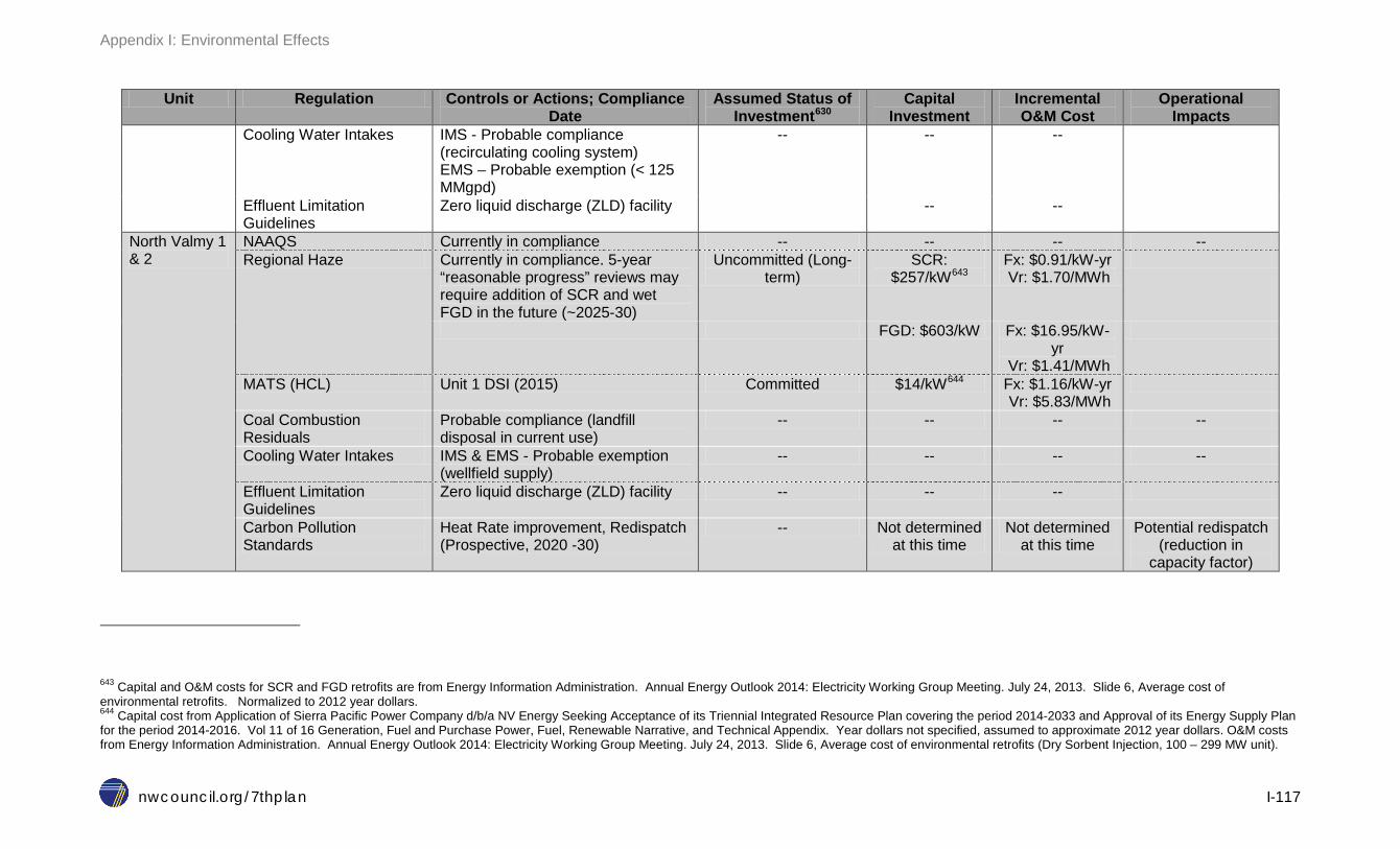
Appendix I: Environmental Effects
nwcouncil.org/7thplan I-117
Unit Regulation Controls or Actions; Compliance Date
Assumed Status of Investment630
Capital Investment
Incremental O&M Cost
Operational Impacts
Cooling Water Intakes IMS - Probable compliance (recirculating cooling system) EMS – Probable exemption (< 125 MMgpd)
-- -- --
Effluent Limitation Guidelines
Zero liquid discharge (ZLD) facility -- --
North Valmy 1 & 2
NAAQS Currently in compliance -- -- -- -- Regional Haze Currently in compliance. 5-year
“reasonable progress” reviews may require addition of SCR and wet FGD in the future (~2025-30)
Uncommitted (Long-term)
SCR: $257/kW643
Fx: $0.91/kW-yr Vr: $1.70/MWh
FGD: $603/kW Fx: $16.95/kW-yr
Vr: $1.41/MWh
MATS (HCL) Unit 1 DSI (2015) Committed $14/kW644 Fx: $1.16/kW-yr Vr: $5.83/MWh
Coal Combustion Residuals
Probable compliance (landfill disposal in current use)
-- -- -- --
Cooling Water Intakes IMS & EMS - Probable exemption (wellfield supply)
-- -- -- --
Effluent Limitation Guidelines
Zero liquid discharge (ZLD) facility -- -- --
Carbon Pollution Standards
Heat Rate improvement, Redispatch (Prospective, 2020 -30)
-- Not determined at this time
Not determined at this time
Potential redispatch (reduction in
capacity factor)
643 Capital and O&M costs for SCR and FGD retrofits are from Energy Information Administration. Annual Energy Outlook 2014: Electricity Working Group Meeting. July 24, 2013. Slide 6, Average cost of environmental retrofits. Normalized to 2012 year dollars. 644 Capital cost from Application of Sierra Pacific Power Company d/b/a NV Energy Seeking Acceptance of its Triennial Integrated Resource Plan covering the period 2014-2033 and Approval of its Energy Supply Plan for the period 2014-2016. Vol 11 of 16 Generation, Fuel and Purchase Power, Fuel, Renewable Narrative, and Technical Appendix. Year dollars not specified, assumed to approximate 2012 year dollars. O&M costs from Energy Information Administration. Annual Energy Outlook 2014: Electricity Working Group Meeting. July 24, 2013. Slide 6, Average cost of environmental retrofits (Dry Sorbent Injection, 100 – 299 MW unit).

Appendix I: Environmental Effects
nwcouncil.org/7thplan I-118
Unit Regulation Controls or Actions; Compliance Date
Assumed Status of Investment630
Capital Investment
Incremental O&M Cost
Operational Impacts
Columbia Generating Station
Fukushima Upgrades (Ordered)
Mitigation strategies Spent fuel instrumentation Containment vents capable of operating under severe accident conditions
Committed $46/kW645 Not available --
CPRR Rulemaking (In-process)
Accident- capable drywell water injection, or Containment vent filters Actions relating to station blackout, fire, flooding or seismic hazards (NRC)
Uncertain; rulemaking in process
Water injection - $3/kW
Vent filters - $30 - $46/kW646
Not available --
Cooling Water Intakes IM - Probable compliance (recirculating cooling system) EM – Probable exemption (< 125 MMgpd)
-- -- -- --
Effluent Limitation Guidelines
Possible minor impacts -- -- -- --
645 Energy Northwest. Fiscal Year 2015 Columbia Generating Station Long Range Plan, adjusted to 2012 yr dollars. 646 Assuming the Nuclear Energy Institute estimates are in 2014 year dollar values.

DRAFT DRAFT
Appendix I: Environmental Effects
nwcouncil.org/7thplan I-119
Costs of complying with recent and proposed environmental and safety regulations can affect the economics of existing power generation facilities in several ways. Some compliance costs, such as those associated with upgrades to existing effluent ponds are likely to be required irrespective of future plant operation. Obligated compliance costs such as these are equivalent to sunk costs and unlikely to greatly affect decisions regarding future plant operation. In contrast, high capital cost compliance actions required to be undertaken only if a plant continues in service, for example, installation of flue gas desulfurization equipment for regional haze control, can render alternative resource options such as new generation, demand side options or market purchases, more attractive than retrofit for continued operation. Compliance actions with significant variable costs such as sorbent injection for mercury control, will affect dispatch cost and thereby the extent to which the plant can compete in the power market against other power generation facilities or demand-side measures. A plant thus affected may continue to operate, though to a lesser extent than previously.
Compliance actions or combinations of compliance actions potentially affect decisions regarding future plant operation when variable costs increase to a level significantly affecting the number of hours in which a unit can economically dispatch against competing units or when avoidable going forward costs increase to levels comparable to the cost of alternative resource options. In the former case, a unit might continue to serve as an economic source of capacity. In the latter, retirement in favor of more cost-effective resource options might be a preferred course of action. The capacity as well as the energy value of an existing plant must be considered in these comparisons. Wholesale energy market prices do not include capacity value except during resource shortages. Nor do all potential new supply or demand-side resource options supply the capacity value of the coal or nuclear units most affected by recent regulatory actions.
Remaining plant life affects capital investment decisions. Most coal-fired units in the Northwest have been operating 30 to 40 years. Though coal steam-electric plants can operate for 60 years or more, and nuclear operating licenses are routinely extended to 60 years (and potentially 80 years), increasing routine maintenance costs, declining efficiency compared to newer plants, and, for coal units, exhaustion of nearby sources of fuel may limit the attractiveness of investing in compliance actions.
A final consideration is the risk to continued operation of coal units posed by climate change policy. Unlike most environmental and safety regulatory actions, the proposed compliance requirements of the Clean Power Plan are not targeted at individual units. Rather, a mix of demand and supply-side actions are proposed, including a shift of dispatch from coal to gas combined-cycle units. Also, proposed state-level climate policy in Washington and Oregon prohibiting or taxing import of electricity from coal-fired plants would further reduce the value of power from these units.
Table I-4 provides a summary of the estimated significant incremental compliance costs for the major affected Northwest generating units that was included in the Seventh Power Plan analysis. This is an important differentiation from Table I-3 because Boardman, Centralia and J.E. Corette are omitted since these units are scheduled for early retirement or cession of coal-firing.

DRAFT DRAFT
Appendix I: Environmental Effects
nwcouncil.org/7thplan I-120
Table I - 4: Estimated Revenue Requirements Impact of Economically Significant Compliance Actions
Units Action
Assumed Status of Investment
(from Table I-3)647
Capital and Cumulative648 O&M
Costs Colstrip 1 & 2 FGD sieve trays; SOFA,
SNCR, DSI, scrubber; Dry ash disposal, slurry pond lining
Committed + Uncommitted (Near-term)
Capital - $343/kW Fx O&M - $1.96/kW-yr Vr O&M - $1.72/MWh
Colstrip 3 & 4 FGD sieve trays; Dry ash disposal; Slurry pond lining; SCR
Committed + Uncommitted (Near-
term)
Capital - $603/kW Fx O&M - $2.23/kW-yr Vr O&M - $1.23/MWh
Jim Bridger 1 & 2 ACI; SCR Committed + Uncommitted (Near-term)
Capital - $391/kW Fx O&M - $0.96/kW-yr Vr O&M - $3.21/MWh
Jim Bridger 3 ACI ; SCR Committed + Uncommitted (Near-term)
Capital - $340/kW Fx O&M - $0.96/kW-yr Vr O&M - $3.21/MWh
Jim Bridger 4 ACI ; SCR Committed + Uncommitted (Near-term)
Capital - $394/kW Fx O&M - $0.96/kW-yr Vr O&M - $3.21/MWh
North Valmy 1 & 2 DSI (Unit 1 only; estimates have been normalized to include both units) 649
Committed + Uncommitted (Near-term)
Capital - $6.72/kW Fx O&M - $0.56/kW-yr Vr O&M - $2.84/MWh
North Valmy 1 & 2
FGD + SCR Uncommitted (Long-term)
Capital - $860/kW Fx O&M - $18.42/kW-
yr Vr O&M - $5.95/MWh
Columbia Generating Station
Fukushima retrofits (Ordered)
Committed + Uncommitted (Near-term)
Capital - $46/kW Fx O&M – n/a Vr O&M – n/a
647 If the status of the investment is “Committed” or “Uncommitted (Near-term)”, Council staff assumed these compliance actions were fairly certain and therefore the estimates were included in the Regional Portfolio Model (RPM). If the status of the investment is “Uncommitted (Long-term)”, Council staff assumed there was too much uncertainty around both the occurrence of the compliance action and the cost estimates, so these estimates are for illustrative purposes only and were not included in the RPM at this time. 648 If the assumed status is “Uncommitted (Long-term), then the capital cost is representative of that compliance order; however the O&M costs are cumulative and include the “Committed” and “Uncommitted (Near-term)” O&M costs as well. 649 DSI is being installed on Unit 1 for reduction in acid gas emissions. The costs shown, assume that the unit 1 installation brings the entire plant into compliance and are therefore allocated to the full plant capacity.

DRAFT DRAFT
Appendix I: Environmental Effects
nwcouncil.org/7thplan I-121
ENVIRONMENTAL IMPACTS OF ASSOCIATED TRANSMISSION AND APPLICABLE REGULATIONS The development and expansion of electricity transmission infrastructure is, in part, a consequence of the development of generating resources. An analysis of the environmental effects of electricity generation should also consider to some extent the environmental impacts of associated transmission development. These impacts include wildlife disruption and habitat fragmentation, modest water and air quality impacts, adverse effects on scenic and aesthetic qualities, and potential effects on cultural resources.
Transmission facilities may be developed and owned by public or private entities. In the Northwest, around 75 percent of the transmission infrastructure, over 15,000 circuit miles, is owned by the Bonneville Power Administration.650
The most significant impacts associated with transmission infrastructure construction and operations are the effects on wildlife and habitat. Habitat disturbance is the primary impact of transmission lines, although avian electrocution is also a concern with some transmission designs. These impacts have the potential to affect several vulnerable species in the Northwest.
Human activity may cause wildlife disturbance during the construction phase of transmission development. While some degree of disturbance is inevitable during the construction phase, developers can mitigate the impacts by avoiding construction during critical periods, such as nesting or wintering.651 Displacement of species as a result of human activity associated with the construction phase is likely to be temporary. However, land cleared for transmission development may continue to allow increased human access in otherwise undeveloped areas after construction is complete.652
Transmission lines and rights-of-way may also lead to habitat fragmentation, as a result of permanent changes in the vegetation around the infrastructure. Transmission rights-of-way are maintained to keep vegetation from growing to a height that would interfere with the delivery of electricity. The Bonneville Power Administration, for example, typically limits vegetation height in rights-of-way to 10 feet tall.653 Transmission system owners employ a variety of methods to limit vegetation growth, including manual and mechanical cutting, and the use of biological agents and herbicides.654 This change in the vegetative structure may make rights-of-way unsuitable as habitat for some species. Habitat fragmentation causes displaced animals to seek new habitat, leading to
650 http://www.bpa.gov/news/pubs/GeneralPublications/gi-BPA-Facts.pdf 651 Id. 652 http://energy.gov/sites/prod/files/nepapub/nepa_documents/RedDont/EIS-0422-DEIS-2010.pdf. 653 http://energy.gov/sites/prod/files/nepapub/nepa_documents/RedDont/EIS-0285-FEIS-01-2000.pdf at 13. 654 http://energy.gov/sites/prod/files/nepapub/nepa_documents/RedDont/EIS-0285-FEIS-01-2000.pdf

Appendix I: Environmental Effects
nwcouncil.org/7thplan I-122
increased competition for resources. In addition to the removal of vegetation during construction and the maintenance of vegetation during operation, transmission development may introduce non-native or invasive species to previously undisturbed areas.655 Mitigation measures are generally limited to avoiding transmission development in sensitive habitat.
Bird species are the most likely to be impacted by direct contact with the transmission facilities. Because transmission lines are non-insulated, a bird that establishes circuit by contacting the energized line and a grounded structure will be electrocuted.656 Of primary concern are eagles and raptors, which have large wingspans and often nest on transmission infrastructure.657 Avian electrocution risk can be mitigated by simply separating energized lines from grounded objects by a distance greater than the span of the birds.658 Electrocution risk can also be mitigated by burying the lines.659
The species impacted by the construction and operation of transmission infrastructure include big game, birds, ground species, and sensitive plants. Big game such as mule deer, pronghorn and elk are likely to avoid areas of transmission development during the construction phase as a result of increased human activity. These impacts are not generally permanent, because human activity declines after construction is complete and transmission infrastructure does not include the installation of any fences that would impede big game behavior.660 Birds are affected by all stages of transmission development, but the primary impacts appear to be the loss of habitat resulting from the alteration of vegetative structures within rights-of-way. Ground species are similarly affected by the alteration of habitat resulting from transmission development. Several Environmental Impact Statements prepared in support of transmission projects in the Northwest identify a familiar array of species of concern. These species include: the Greater sage grouse, Golden eagle, Ferruginous hawk, Sage sparrow, Preble’s shrew, Merlin, Peregrine falcon, Loggerhead shrike, Black-tailed jackrabbit, Washington ground squirrel, Pygmy rabbit, Mule deer, Northern sagebrush lizard, and Green-tinged paintbrush.661 The siting of a transmission project, its size, and its relation to sensitive habitat determines the precise contours of its wildlife impacts.
Wildlife impacts may be regulated by the ESA, the Migratory Bird Treaty Act and the Bald and Golden Eagle Protection Act. Under the ESA, a private (or public non-federal) transmission developer is typically required to evaluate the proposed site for the presence of listed species or critical habitat. If either are present, the private developer may be required to obtain an incidental take permit from FWS or NOAA Fisheries. If the transmission developer is a federal agency, like the
655 http://teeic.indianaffairs.gov/er/transmission/impact/construct/index.htm 656 http://www.fishwildlife.org/files/AFWA-State_agency_transmission_guide_FINAL.pdf at 15. 657 http://www.fws.gov/southwest/es/documents/R2ES/LitCited/LPC_2012/Steenhof_et_al_1993.pdf. Interestingly, transmission infrastructure may also benefit raptors by providing a nesting substrate. 658 http://www.fishwildlife.org/files/AFWA-State_agency_transmission_guide_FINAL.pdf 659 http://www.blm.gov/or/districts/prineville/plans/wbw_power_row/files/wbw_power_row_final_EIS.pdf at ES-11 660 http://www.blm.gov/or/districts/prineville/plans/wbw_power_row/files/wbw_power_row_final_EIS.pdf 661 http://energy.gov/sites/prod/files/nepapub/nepa_documents/RedDont/EIS-0422-DEIS-2010.pdf at S-19. http://www.blm.gov/or/districts/prineville/plans/wbw_power_row/files/wbw_power_row_final_EIS.pdf at ES-7.

Appendix I: Environmental Effects
nwcouncil.org/7thplan I-123
Bonneville Power Administration, compliance with the ESA requires consultation with FWS or NOAA Fisheries. If a biological assessment reveals the presence of a listed species or critical habitat, FWS or NOAA Fisheries are required to prepare a biological opinion that determines whether the proposed action is likely to jeopardize the continues existence of a listed species. If the relevant agency makes a “no jeopardy,” it may authorize the action and recommend reasonable prudent measures to avoid take. Incidental take by federal entities authorized to act by the FWS or NOAA Fisheries is permitted. A jeopardy determination by FWS or NOAA Fisheries forecloses a federal entity’s authority to act. The MBTA and BGEPA may also impose some limitations on transmission development, by requiring a transmission developer to cooperate with FWS to implement ACPs to limit impacts to eagles and mitigate migratory bird take.
The construction and operation of transmission infrastructure has modest effects on water quality and air quality impacts are limited to the construction phase. During the construction phase, the potential water quality impacts result from the removal of vegetation, excavation, grading and trenching required to prepare a site for transmission lines. These processes increase soil erosion, which leads to a rise in sediment loads in nearby waterways. Trenching and the construction of access roads may also alter drainage patterns, resulting in decreased water absorption by soil and more rapid runoff during precipitation or snowmelt.662 Vehicular traffic during construction and maintenance may also lead to the introduction of oils and heavy metals into previously undisturbed waters. In addition, the development of transmission facilities typically requires the withdrawal of water from adjacent waterways for dust control. The operation of transmission infrastructure requires maintenance of the vegetation within transmission rights-of-way, which typically involves the application of herbicides and biological agents.663 Rain may cause these chemicals to wash into adjacent waterways.664 Taking steps to maintain the natural drainage patterns of a waterway, such as limiting the channelization of streams into culverts, can mitigate water quality impacts. In addition, water and sediment control measures (hay bales) can be used in trenches to limit sediment loads and slow runoff.665
To the extent that stormwater is channelized and discharged into adjacent surface waters during the development of a transmission project, developers must obtain a § 402 NPDES permit from the EPA. In addition, the construction of transmission infrastructure in wetlands requires a developer to seek a §404 dredge and fill permit from the Corps. The Corps has developed a Nationwide Permit that streamlines the § 404 permitting process for many activities associated the development of utility infrastructure.666
Transmission projects typically only cause air quality impacts during the construction phase. The construction phase of transmission development typically involves blasting and the use of heavy
662 http://teeic.indianaffairs.gov/er/transmission/impact/construct/index.htm 663 http://energy.gov/sites/prod/files/nepapub/nepa_documents/RedDont/EIS-0285-FEIS-01-2000.pdf at 11. 664 http://teeic.indianaffairs.gov/er/transmission/impact/construct/index.htm. 665 http://energy.gov/sites/prod/files/nepapub/nepa_documents/RedDont/EIS-0422-DEIS-2010.pdf at S-21. 666 http://www.usace.army.mil/Portals/2/docs/civilworks/nwp/2012/NWP_12_2012.pdf

Appendix I: Environmental Effects
nwcouncil.org/7thplan I-124
machinery, resulting in exhaust from construction equipment, and fugitive dust from blasting, excavation and road construction.667 Air impacts rarely persist beyond construction.
The construction and operation of transmission infrastructure may result in aesthetic harms, human health concerns, and the potential disruption of cultural and historical resources. Transmission lines have the potential to create new visual features in previously undeveloped areas, which may be unwelcome to adjacent landowners and people seeking natural or scenic character.668 Project developers can mitigate these impacts to some degree by avoiding visually sensitive areas, siting transmission lines in previously disturbed areas, preserving a vegetative buffer along rights-of-way, and using non-reflective materials in building transmission infrastructure.669 In addition to the visual impacts connected to transmission infrastructure, the operation of transmission facilities produces electric and magnetic fields. While members of the public have expressed some concern over the health impacts of these fields, scientific studies have not demonstrated any causal connection between exposure to electromagnetic fields and cancer or other disease.670 Electromagnetic fields do have the potential to interfere with certain implantable medical devices, such as pacemakers, but the strength of an electromagnetic field decreases rapidly as distance from the source increases.671
The cultural and historical impacts of transmission infrastructure may include the visual or physical disturbance of important resources. Transmission lines may create a new visual feature in places of cultural or historical significance, diminishing the value of the resource for people who seek to experience it. Cultural resources may include sacred tribal lands; historical resources may include historic trails and sites. These harms can be largely mitigated using the same measures discussed in the paragraph describing aesthetic harms above. Additionally, project developers should consult with relevant tribes and state agencies regarding the locations of resources of particular value and seek to avoid disruptive development near those areas.672 The construction of transmission infrastructure may reveal artifacts of cultural or historical significance or turn up sites of archeological importance. The potential impacts of these discoveries can be mitigated through the development of a discovery plan that outlines the appropriate steps for crewmembers to take in notifying the relevant tribes, state agencies and law enforcement.673
Whether developed by a federal or non-federal entity, transmission development typically includes sufficient federal involvement to trigger the NEPA’s environmental analysis requirements. Depending on the scope of the impacts, project developers may be required to assist a federal agency in preparing a relatively basic EA or a significantly more comprehensive EIS. The NEPA process does
667 http://teeic.indianaffairs.gov/er/transmission/impact/construct/index.htm 668 http://www.blm.gov/or/districts/prineville/plans/wbw_power_row/files/wbw_power_row_final_EIS.pdf 669 http://energy.gov/sites/prod/files/nepapub/nepa_documents/RedDont/EIS-0422-DEIS-2010.pdf at S-23. 670 http://www.niehs.nih.gov/health/materials/electric_and_magnetic_fields_associated_with_the_use_of_electric_power_questions_and_answers_english_508.pdf at 16-27 671 http://www.niehs.nih.gov/health/topics/agents/emf/ 672 http://energy.gov/sites/prod/files/nepapub/nepa_documents/RedDont/EIS-0422-DEIS-2010.pdf at S-23. 673 Id.

Appendix I: Environmental Effects
nwcouncil.org/7thplan I-125
not impose any substantive responsibilities on transmission developers, beyond allowing public input and requiring an analysis of all reasonable alternatives.
Decisions on whether and where to site a transmission line are largely in the domain of the federal land managing agencies, if the line will be on federal land, or in state agencies designated to approve the siting of energy facilities, such as Oregon’s Energy Facility Siting Council (part of the Oregon Department of Energy), if on private land. Federal land management laws and regulations, such as the Federal Land Policy and Management Act (FLPMA), the National Forest Management Act, and the Columbia River Gorge National Scenic Act, provide some measure of protection against and mitigation for environmental effects beyond the NEPA environmental analysis and the specific substantive requirements of laws such as the ESA, MBTA and BGEPA. The same is true of state energy siting and land use laws and regulations that apply to decisions by the state energy siting agencies. A complicated mix of federal and tribal laws and regulations apply to decisions to allow development of transmission lines on the lands of the Indian tribes in the Northwest.
State-federal cooperation in this area occurs in a number of ways. A key driver was a provision in FLPMA in 1976 that required federal agencies to comply with state environmental protection standards in approving right-of-ways across federal public lands for transmission lines and similar projects. Uncertainty over the precise dimensions of this obligation led to litigation the 1980s between states and, in particular, Bonneville, over the development of transmission lines, with the federal courts largely agreeing with the states about the importance of ensuring consideration of and compliance with state environmental protection regulations in approving transmission rights-of-ways.674 Coupled with the new Northwest Power Act, and uncertainty under that Act as to the extent the regional Columbia River Basin Fish and Wildlife Program should address transmission system impacts to wildlife, led Bonneville and the Northwest states to execute cooperative agreements in the 1980s regarding transmission corridors, transmission line development, and impacts to wildlife. The agreements were intended in large part to assure the appropriate consideration and application of state environmental protections in federal transmission developments. These agreements remain in effect today. The Council has recognized these agreements as a key tool in the way the regional power system should consider, protect against and mitigate for wildlife impacts in transmission system development. It is important that implementation of the agreements and the application of state and federal environmental regulations continues and is effective in addressing impacts to wildlife and other environmental qualities.675
State and federal fish and wildlife agencies and Indian tribes expressed concerns during the process in 2013-14 for amending the Council’s Fish and Wildlife Program over the cumulative impacts to wildlife from transmission development in the Pacific Northwest, especially in the light of the recent expansion of transmission infrastructure to support renewable energy development, especially wind
674 Columbia Basin Land Protection Association v. Schlesinger (9th Cir 1981) involved the development of the Lower Monumental-Ashe transmission line in eastern Washington. Montana v. Johnson (9th Cir 1984), concerned the development by Bonneville of a transmission line from Townsend to Hot Springs, in northwestern Montana, associated with the building of the Colstrip coal plant. 675 See 2014 Columbia River Basin Fish and Wildlife Program, Appendix S, http://www.nwcouncil.org/media/7148962/2014-12appendixs.pdf, at 283.

Appendix I: Environmental Effects
nwcouncil.org/7thplan I-126
projects.676 The Northwest Power Act and the fish and wildlife program and power plans developed under the Act provide a comprehensive regional protection and mitigation program to address the cumulative impacts of existing hydroelectric generating resources on fish and wildlife, as well as provide the opportunity to protect areas from further hydroelectric development and to consider the environmental effects and costs of all new generating resources in deciding which to acquire. Similar comprehensive regional laws and programs do not to exist to address the cumulative effects of and mitigate for transmission development or renewable energy development, or to provide for comprehensive and enforceable protected areas for transmission and renewable energy development. Also, the Council’s power planning authority does not include planning for the development of transmission infrastructure or the ability to include in the plan enforceable provisions regarding the acquisition of or the decisions to approve transmission lines. Associated transmission development is instead part of the life-cycle costs (including environmental costs) and matters of environmental quality to be considered in analyzing and comparing the costs of new resource alternatives. See Chapter 19. It is unclear at this point whether the existing federal and state mechanisms to address environmental effects of transmission development, especially including effects to wildlife, are not adequate to address the concerns raised by the wildlife managers, and if inadequate, what can be done to improve this situation. The Council is committing, in an Action Plan item, to helping the fish and wildlife agencies and Indian tribes to work with the entities and agencies involved in developing, operating, and regulating transmission infrastructure to explore these concerns further. This investigation may also assist the Council in future power plans in considering the environmental issues raised by the transmission development associated with new resource development. And most important, avoiding the environmental impacts of transmission is another of many considerations supporting the aggressive development of cost-effective energy efficiency and demand response measures in the plan’s resource strategy.
676 Id., at 283, 329-30.

Appendix I: Environmental Effects
nwcouncil.org/7thplan I-127
ACRONYMS AND ABBREVIATIONS Acronym Meaning ACI Activated Carbon Injection ACP Advanced Conservation Practices BART Best Available Retrofit Technology BGEPA Bald and Golden Eagle Protection Act BLM Bureau of Land Management BPT Best Practicable Control Technology Currently Available BTA Best Technology Available CAA Clean Air Act CaBr2 Calcium Bromide Treatment of Coal CCR Coal Combustion Residuals CCS Carbon Capture and Sequestration CE Categorical Exclusions CGS Columbia Generating Station CO2 Carbon Dioxide Corps Army Corps of Engineers CREP Community Renewable Energy Projects (Montana RPS) DESP Dual Electrostatic Precipitators DSI Dry Sorbent Injection EA/FONSI Environmental Assessment and Finding of No Significant Impact EIA Energy Information Administration EIS Environmental Impact Statements EMS Entrainment Mortality Standards EPA Environmental Protection Agency ESA Endangered Species Act ESP Electrostatic Precipitator FERC Federal Energy Regulatory Commission FGD Flue Gas Desulfurization FIP Federal Implementation Plan FWS Fish and Wildlife Service GWP Global Warming Potential HNO3 Nitric Acid IMS Impingement Mortality Standards Li-ion Lithium Ion Li-NCM Lithium Nickel Cobalt Manganese Oxide LNB Low NOx Burners MATS Mercury and Air Toxics Standards MBTA Migratory Bird Treaty Act MOFA Modified Overfire Air MSHA Mine Safety and Health Administration NAAQS National Ambient Air Quality Standards NaS Sodium-sulfur NEPA National Energy Policy Act of 1969 NESHAP National Emissions Standards for Hazardous Air Pollutants N2 Diatomic Nitrogen N2O Nitrous Oxide NO Nitric Oxide NO2 Nitrogen Dioxide

Appendix I: Environmental Effects
nwcouncil.org/7thplan I-128
NOx Shorthand reference to nitrogen oxides, but may specifically refer to NO and NO2 NOAA National Oceanic and Atmospheric Administration NPDES National Pollutant Discharge Elimination System NRC Nuclear Regulatory Commission NSPS New Source Performance Standards OFA Overfire Air OSMRE Office of Surface Mining, Reclamation and Enforcement PAC Powdered Activated Carbon PM Particulate Matter PTC Production Tax Credit PV Solar photovoltaic RCRA Resource Conservation and Recovery Act REC Renewable Energy Credit/Renewable Energy Certificate RPM Regional Portfolio Model RPS Renewable Portfolio Standards SCR Selective Catalytic Reduction SIP State Implementation Plan SMCRA Surface Mining Control and Reclamation Act SMR Small Modular Reactors SNCR Selective Non-catalytic Reduction SO2 Sulfur Dioxide SOFA Separated Overfire Air ULSD Ultra Low Sulfur Distillate VOC Volatile Organic Compound WECC Western Electricity Coordinating Council ZLD Zero Liquid Discharge

Seventh Northwest Conservation and Electric Power Plan
nwcouncil.org/7thplan J-1
APPENDIX J: DEMAND RESPONSE RESOURCES – BACKGROUND INFORMATION
Contents Overview ........................................................................................................................................... 2 General Methodology and Assumptions ............................................................................................ 2
Demand Response Resources Assessment Methodology ............................................................. 2 Calculate Total Resource Cost by Programs .............................................................................. 3 Calculate Potential by Reference Resource ............................................................................... 5
Other Resource Attributes.............................................................................................................. 6 Reference Resource Parameters ...................................................................................................... 7
Input Parameters ........................................................................................................................... 7 Existing Demand Response in the Region ........................................................................................ 9
Current Demand Response Programs ........................................................................................... 9 Current Pilot Programs ................................................................................................................ 11
List of Figures and Tables Equation J - 1: Levelized Enablement Cost Calculation for New Potential ......................................... 4 Equation J - 2: Real Levelized Enablement Cost in 2012 dollars ....................................................... 4 Equation J - 3: Net Real Levelized Implementation Cost in 2012 dollars ........................................... 5 Table J - 1: Demand Response Reference Resource Parameters in the RPM .................................. 8 Table J - 2: Seasonal Percentages of Total Potential by DR Reference Resource ............................ 9
Appendix J: Demand Response Resources
nwcouncil.org/7thplan J-2
OVERVIEW This appendix provides an overview of the general methodology used by the Council for estimating the costs and sources of demand response potential in the region. This methodology was used to develop the inputs for demand response (DR) resources in the Regional Portfolio Model (RPM).1 In the RPM, demand response potential for the region was partitioned into four resources, with individual programs aggregated by levelized cost into a particular demand response resource. The development of the aggregate demand response resource characteristics for each of the four resources is available via spreadsheet on the Council’s Seventh Power Plan web site: http://www.nwcouncil.org/energy/powerplan/7/technical.
In addition, this appendix also provides a description of demand response programs (long-term and pilot) in the region. These existing programs and pilot efforts, referenced in Chapter 14, show the direction of demand response in the region and help provide narrative for the varying capabilities of demand response that are not currently modeled in the RPM.
GENERAL METHODOLOGY AND ASSUMPTIONS As described in Chapter 14, the Council prioritized firm demand response potential in the Pacific Northwest during the 20-year power planning period, per input from the Systems Analysis Advisory Committee and the Pacific Northwest Demand Response Project industry experts. DR resources allowing load curtailments directly controlled by the utility or scheduled ahead of time are considered to be firm. Non-firm DR resources are outside of the utility’s direct control, since the curtailments are based on customer response to pricing signals. Non-firm DR resources have a less clearly understood reliability level for meeting a system peak hour need, and since one of the reasons the RPM might select a new resource is based on single-hour peak capacity adequacy, it is reasonable to solely use firm resources in the Seventh Power Plan. In addition, part of the consideration for how the RPM would select resources was based on the fact that a reference DR resource could be dispatched similarly to a reference generation plant,2 a mechanism more representative of firm DR resources. Non-firm demand response programs have been tested in the region and some utilities have programs. Some of these are described in more detail in the section on existing and pilot DR programs.
Demand Response Resources Assessment Methodology Since demand response has some of the characteristics of conservation (demand-side) and generation resources (dispatchable), the methodology for defining the DR resources for assessment in the Seventh Power Plan is a hybrid of the techniques used for developing conservation and generation resources.3 Per the narrative in Chapter 14, the 11 types4 of DR programs studied in the
1 See Appendix L for more detail on the RPM. 2 Reference plant is defined in Appendix H. 3 See Appendix G for the conservation resources methodology and Appendix H for the generating resources methodology.
Appendix J: Demand Response Resources
nwcouncil.org/7thplan J-3
Council’s regional DR Program Potential Study5 varied over three sectors, two dispatch technologies, and various seasonal profiles. Accounting for all the permutations,6 there were 19 distinct programs with different cost information for each. However, similarly to conservation and generation resources, there is a limit to the number of DR resources that the Council can evaluate in the RPM.7
Demand response is modeled in the RPM as four reference DR resources that represent the quantity of technically achievable demand response available in each model decision period8 from 2016 to 2035. The reference resources are generated by sorting the individual DR programs into four cost bins, based on their real levelized Total Resource Costs (TRC). In the RPM, similarly to how the reference generating resources are modeled, each of the reference DR resources has a quarterly shape for both capacity and energy, levelized cost for installing the resource (enablement costs), levelized cost for maintaining the resource (implementation cost), a maximum achievable ramp per decision period, and maximum acquisition by the end of the study.
Calculate Total Resource Cost by Programs
Total resource cost for DR resources is the made up of enablement and implementation costs. Sources of the raw data used to calculate the enablement and implementation costs are summarized in Appendix A of the Council’s DR Program Potential Study5 and the calculations are in a spreadsheet on the Council’s website: http://www.nwcouncil.org/energy/powerplan/7/technical.9
Enablement Cost
Enablement costs represent the cost to purchase and install the technology divided by the standard load reduction. Enablement costs are similar to construction costs for a reference generation plant, and are input similarly into the RPM. However, unlike the fairly well known lifetime assumptions for generating plants and conservation measures, there was mixed information from stakeholders about
4 A type of program is determined by its load reduction source. The 11 types of DR programs considered in the Council’s analysis are as follows: residential space and water heating, residential central and room air conditioning, space cooling for small and medium size commercial customers, commercial lighting controls, irrigation pumping, curtailable/interruptible tariffs, load aggregation, and refrigerated warehouses. 5 The Navigant Potential Report, “Assessing Demand Response (DR) Program Potential for the Seventh Power Plan”, was delivered as a document and a supporting spreadsheet, NPCC_Assessing DR Potential for Seventh Power Plan_UPDATED REPORT_1-19-15.pdf and NPCC_7thPowerPlan_DR_Programs_UPDATE_2015 01 16.xlsx, respectively. 6 See Table 14-2: Demand Response Programs Studied for the different programs by sector, technology and seasonality. 7 Recall per discussions in Appendices G and L that the RPM run time increases significantly with each new resource added, so parsimony is required when resources for assessment are input to the model. 8 A decision period in the RPM for generating and DR resources is annually in quarter 1 from 2016 through 2021, and biannually in quarter 1 from 2023 through 2035. 9 DR Input assumptions: DRPotential_PostAprCouncil_ForWebsite_05042015.xlsx

Appendix J: Demand Response Resources
nwcouncil.org/7thplan J-4
the lifetime of the technology with respect to customer participation in the DR program. In other words, although the device could last longer, due to customer turnover, there may be multiple installations and uninstalls within the 20-year plan period. The Council’s assumption was to give each device a five-year lifetime, the minimum of the range of device/participation lifetimes recommended by stakeholders. The levelized enablement cost calculation is summarized in Equation J-1.
Equation J - 1: Levelized Enablement Cost Calculation for New Potential
𝐿𝐸𝐶𝑗 = �∑ (𝑇𝑒𝑐ℎ𝑛𝑜𝑙𝑜𝑔𝑦 𝐶𝑜𝑠𝑡 + 𝐼𝑛𝑠𝑡𝑎𝑙𝑙𝑎𝑡𝑖𝑜𝑛 𝐶𝑜𝑠𝑡)𝑖(𝑁𝑢𝑚𝑏𝑒𝑟 𝑜𝑓 𝑐𝑢𝑠𝑡𝑜𝑚𝑒𝑟𝑠)𝑖
(1 + 𝑟)𝑖5𝑖=1
∑ (𝐿𝑜𝑎𝑑 𝐼𝑚𝑝𝑎𝑐𝑡)𝑖(𝑁𝑢𝑚𝑏𝑒𝑟 𝑜𝑓 𝑐𝑢𝑠𝑡𝑜𝑚𝑒𝑟𝑠)𝑖(1 + 𝑟)𝑖
51
�
𝑗
Where r is the Council’s discount rate,10 j is a year between 2016 and 2035
Participation in the all DR programs is assumed to be persistent, factoring the turnover rate in the Council’s Potential study,11 the real levelized cost (in 2012 dollars) to enable both the new potential and the potential that requires a reinstall of equipment is summarized in Equation J- 2.
Equation J - 2: Real Levelized Enablement Cost in 2012 dollars
𝑅𝑒𝑎𝑙 𝐿𝑒𝑣𝑒𝑙𝑖𝑧𝑒𝑑 𝐸𝑛𝑎𝑏𝑙𝑒𝑚𝑒𝑛𝑡 𝐶𝑜𝑠𝑡 �𝑖𝑛 $
𝑘𝑊 ∙ 𝑦𝑒𝑎𝑟�= � (1 + 𝐼)(2016−2012)�(𝐿𝐸𝐶)𝑗 + (𝐿𝐸𝐶)𝑗−5�
2035
𝑗=2016
Where I is the Council’s inflation rate12
Implementation Cost
Implementation costs represent the costs to market DR, research new DR opportunities, pay support staff, and pay customers capacity reserve incentives. In Equation J-3 below, net real levelized implementation costs are calculated by considering the implementation costs netted with a transmission deferral credit (26 dollars per kilowatt year, in real 2012 dollars). The justification for the transmission deferral credit for a reference demand response resource is similar to the justification provided in Appendix G13 for conservation measures, in that upgrades or expansions to the transmission system may be deferred by the reduction in peak demand. Unlike conservation resources, demand response resources did not receive a credit for deferring distribution system upgrades or expansions, since it was assumed that the distribution system would need to be capable of serving the customers peak demand at times when the DR resource was not dispatched. The implementation costs for DR resource are similar to the fixed operations and maintenance costs for a reference generation plant in that these costs are reoccurring and necessary to maintain a properly functioning resource, and are input similarly into the RPM.
10 Council’s discount rate assumption is 4%, see Appendix A for more information. 11 Turnover rate from assumption from Council’s Potential Study is 1% per annum. 12 Council’s inflation rate assumption is 1.64%. 13 See the Appendix G: Benefits of Conservation section.

Appendix J: Demand Response Resources
nwcouncil.org/7thplan J-5
Equation J - 3: Net Real Levelized Implementation Cost in 2012 dollars
𝑅𝑒𝑎𝑙 𝐿𝑒𝑣𝑒𝑙𝑖𝑧𝑒𝑑 𝑁𝑒𝑡 𝐼𝑚𝑝𝑙𝑒𝑚𝑒𝑛𝑡𝑎𝑡𝑖𝑜𝑛 𝐶𝑜𝑠𝑡 �𝑖𝑛 $
𝑘𝑊 ∙ 𝑦𝑒𝑎𝑟�=
(1 + 𝐼)(2016−2012) �∑ (𝐼𝑚𝑝𝑙𝑒𝑚𝑒𝑛𝑡𝑎𝑡𝑖𝑜𝑛 𝐶𝑜𝑠𝑡 − 𝑇𝐷 𝐷𝑒𝑓𝑒𝑟𝑟𝑎𝑙 𝐶𝑜𝑠𝑡)𝑖(𝑃𝑜𝑡𝑒𝑛𝑡𝑖𝑎𝑙 𝑖𝑛 𝑘𝑊)𝑖
(1 + 𝑟)𝑖20𝑖=1
∑ (𝑃𝑜𝑡𝑒𝑛𝑡𝑖𝑎𝑙 𝑖𝑛 𝑘𝑊)𝑖(1 + 𝑟)𝑖
201
�
𝑗
Where I is the Council’s inflation rate12
Total Resource Cost
The total resource cost was used to sort the 19 DR programs into cost bins that make up the four reference DR resources. The total resource cost is the sum of the real levelized enablement cost and the net real levelized implementation cost of the resource in 2012 dollars per kilowatt-year. The total resource cost for each DR reference resource is calculated by taking a weighted average total resource cost for each resource.14
Calculate Potential by Reference Resource
The technical potential available in a particular season associated with each reference DR resource is calculated by summing the total technical potential from each of the programs15 that make up a particular reference resource.
Seasonal Peak Capacity
The DR programs that make up the reference resources have diverse seasonal shapes.16 Each of these reference resources has a seasonal peak capacity percentage that accurately depicts the megawatts available from each reference resource. The seasonal peak capacity percentage is calculated by summing the total available potential from each program in the reference resource in each season and dividing it by the total technical potential in each resource (regardless of season). Thus, when the seasonal peak capacity percentage is multiplied by the total technical potential available for a resource in a decision period, the result is the appropriate seasonal capacity that proportionally represents the programs that make up the reference DR resource.
Seasonal Energy
Since the actual DR programs have a different number of total dispatch hours possible, the Council determined a representative number of total dispatch hours by reviewing proxy programs considered in recent regional utility resource plans and existing DR programs, where available. Then, for each
14 See Figure 14-1: Demand Response Programs and Cost Bins (2012$ per kW-year) in Chapter 14 for graphic representation of the weighted average costs in each bin. 15 Note that the assumption is that there is no interaction between programs, so their potential can be summed without adjustment. 16 See Tables 14-3 through 14-6 in Chapter 14 for examples of the seasonal diversity in the reference resources.

Appendix J: Demand Response Resources
nwcouncil.org/7thplan J-6
of these 19 distinct programs in the Council’s DR Program Potential study, a total associated seasonal energy was calculated by multiplying the percentage of hours the resource could be dispatched in the quarter by the total megawatts available in that quarter.17 Note that DR programs focused on refrigerated warehouses, irrigation pumping, and water heating are primarily load-shifting resources, so there is assumed to be no net load reduction by quarter.
Then, the resulting quarterly energy for the DR reference resource is calculated by taking a weighted average quarterly energy for each DR program in that reference resource. This seasonal energy for each reference DR resource is used to represent the limited hours of dispatch by season that proportionally represent the programs that make up the reference DR resource.
Other Resource Attributes The following other attributes are used to describe the reference demand response resources for the Seventh Power Plan. These attributes are similarly defined as the attributes for a reference generation plant,2 since both resource types are input similarly into the RPM. The input assumptions by each DR reference resource are provided in Table J-1.
Location - The general geographic location of the reference resource, which is important in properly accounting for transmission costs.
Earliest In-Operation Date (Year) - The earliest date a reference resource is assumed to be in operation, taking into account program development and device installation. The RPM cannot select the resource before this date.
Program Lead Time - The amount of time it takes to get one or many DR programs up and running. This is the lead time to hire and train staff, begin marketing, and assess DR implementation strategy.
Economic Life (Years) - The assumed useful operating life of the resource for accounting purposes.
Resource Size (megawatts) - The DR reference resource size as it is acquired by the RPM. Note that there is no standard size for a DR resource, and this designation is for modeling ease and computation time.
Planning Costs – These are the costs connected with getting a one or many DR programs up and running during the program lead time period in real levelized dollars per kilowatt year. These are associated with paying implementation costs without considering transmission deferral credit and capacity incentive payments for the program lead time.
17 See the DR Input assumptions, “ DRPotential_PostAprCouncil_ForWebsite_05042015.xlsx” on the ‘CostByType_Details’ and ‘EnergyCalculations’ worksheets on the Council website http://www.nwcouncil.org/energy/powerplan/7/technical for more details.

Appendix J: Demand Response Resources
nwcouncil.org/7thplan J-7
Dispatch Cost (dollars per megawatt-hour) - An estimate of the variable operation cost for the reference resource, including all costs that are a function of the amount of power curtailed. This most closely represents variable customer incentives focused on dispatch of the DR resource.
Maximum Technical Potential - For modeling purposes in RPM, this constraint represented the maximum amount of technical potential, calculated for each reference resource that could be developed over the course of the study. This maximum technical potential represents the sum of the maximum technical potential of each program that makes up the reference resource.
Maximum Build Rate per Decision Period – The maximum megawatts that can be subscribed between decision periods in the RPM.
REFERENCE RESOURCE PARAMETERS Input Parameters For each DR reference resource, general and seasonal inputs defined in the sections above are input into the RPM per Table J-1 and Table J-2, respectively. Recall that the seasonal capacity percentage when multiplied by the total resource acquired (in megawatts) represents the seasonal peak capacity capability (in megawatts) of the reference resources. Similarly, the seasonal energy percentage when multiplied by the total resource acquired (in megawatts) represents the seasonal energy (in average megawatts) associated with the quarterly dispatch of the reference resources.

Appendix J: Demand Response Resources
nwcouncil.org/7thplan J-8
Table J - 1: Demand Response Reference Resource Parameters in the RPM
Reference Resource Cost Bin 1 Cost Bin 2 Cost Bin 3 Cost Bin 4
Location West side18 West side West side West side Earliest Operation
Year 2016 2016 2016 2016
Program Lead Time (Months) 6 6 6 6
Economic Life (Years) 5 5 5 5
Resource Size (MW) 10 10 10 10
Planning Costs ($/kW-yr) 7 9 8 10
Enablement Costs ($/kW-yr) 3 47 60 109
Implementation Cost ($/kW-yr) 22 9 17 35
Dispatch Cost ($/MWh) 110 110 110 110
Maximum Technical Potential (MW) as modeled
1,520 1,220 400 1,210
Maximum Build Rate per Decision Period (MW) as
modeled
220 180 60 170
18 A majority of the demand in the region and benefit of transmission deferral is on the west side; however, in practice demand response programs can be and are on the east side. Current RPM modeling methodology does not allow the Council to let resources be considered a percentage of east or west side resources, which might better represent a reference demand response resource.

Appendix J: Demand Response Resources
nwcouncil.org/7thplan J-9
Table J - 2: Seasonal Percentages of Total Potential by DR Reference Resource
Quarter 119 Quarter 2 Quarter 3 Quarter 4 Seasonal
Percentage Capacity Energy Capacity Energy Capacity Energy Capacity Energy
Cost Bin 1 96% 0.7% 0% 0.0% 100% 1.4% 96% 0.6% Cost Bin 2 97% 0.4% 0% 0.0% 73% 0.2% 97% 0.4% Cost Bin 3 14% 0.0% 0% 0.0% 100% 2.2% 14% 0.0% Cost Bin 4 67% 0.7% 0% 0.0% 38% 0.7% 67% 0.7%
EXISTING DEMAND RESPONSE IN THE REGION During the public process of developing the inputs of the Seventh Plan, questions have arisen about the viability and achievability of demand response in the region. Since, historically, the capability of the regional hydropower system has been sufficient to serve the region’s peak demand needs that perspective is understandable. However, during the Western US Energy Crisis of 2000 and 2001, when wholesale electricity prices skyrocketed, Pacific Northwest significantly expanded its DR capability. There have not been similar price spikes and peak period supply shortages in the time since, and demand response capability in the region has diminished. This section provides a context for the current state of demand response in the region.
Current Demand Response Programs Idaho Power
As of 2015, Idaho Power maintains approximately 390 megawatts of total demand response capability in the region. Idaho Power’s loads peak in the summer, so the three active programs are focused in the summer.
The Irrigation Peak Rewards Program20 allows irrigators that have existing load control devices installed to remotely turn off specific irrigation pumps to receive a financial incentive from Idaho Power. The load control events can occur Monday through Saturday between 1 p.m. and 8 p.m. from June 15th through August 15th. The program can be used up to four hours a day, 15 hours a week, and 60 hours a season. This program has a fixed-incentive payment structure (demand credit in dollars per kilowatt and energy credit in dollars per kilowatt-hour) and a variable-incentive payment (in dollars per event kilowatt hour) after the first three events. Note that this program design is similar to the modeling of proxy irrigation programs, initiated by basic or automated switching technology, in the list of potential future demand response programs in the region.
19 Quarter 1 is defined to be January, February, and March; Quarter 2 is defined to be April, May, and June; Quarter 3 is defined to be July, August, and September; and Quarter 4 is defined to be October, November, and December. 20 https://www.idahopower.com/pdfs/EnergyEfficiency/Irrigation/Programs/PeakRewards/summary.pdf

Appendix J: Demand Response Resources
nwcouncil.org/7thplan J-10
The Flex Peak Program21 allows large commercial and industrial customers to reduce a set amount of electrical load when Idaho Power initiates a demand response event. The load control events can occur Monday through Saturday between 2 p.m. and 8 p.m. from June 15th through August 15th. The program can be used up to four hours a day, 15 hours a week, and 60 hours a season. This program has a fixed capacity payment structure (demand credit in dollars per weekly kilowatt reduction) and a variable energy payment (in dollars per event kilowatt hour of the event) after the first three events. Participants are notified two hours prior to the event to ensure there is time for the demand reductions to be completed by the beginning of the event. Note that this program design is similar to the modeling of proxy curtailable/interruptible tariffs, lighting, or refrigerated warehouse programs, in the list of potential future demand response programs in the region.
The A/C Cool Credit Program22 allows residential customers with the installed equipment required to support A/C cycling to cycle their air conditioning during peak demand periods in the summer. The A/C can be cycled off for a portion of the hour during each hour of a peak period (up to four hours) from June 15th through August 15th. Participants receive a fixed $5 credit on their bill for each of the three months they are enrolled in the program. Note that this program design is similar to the modeling of proxy residential space cooling programs for central air conditioning units with programmable communicating thermostats, in the list of potential future demand response programs in the region.
Pacific Power
As of 2015, Pacific Power (Rocky Mountain Power in Idaho) has approximately 170 megawatts of irrigation load control23 for Idaho customers with at least 25 horsepower irrigation pumps. The load control events can occur Monday through Saturday between 12 p.m. and 8 p.m. from June 1st through August 15th. The program can be used up to four hours a day, 12 hours a week, and 52 event hours a season. In addition, there is a maximum of one event per day and 20 events per season. This program has a fixed-incentive payment structure (demand credit in dollars per kilowatt) that is set by average available load from the customer’s pumps. Note that this program design is similar to the modeling of proxy irrigation programs, initiated by basic or automated switching technology, in the list of potential future demand response programs in the region.
Portland General Electric
As of 2015, Portland General Electric (PGE) has approximately 28 megawatts of DR capability from a residential Time-Of-Use pricing program,24 commercial and industrial Demand Buyback Rider program,25 and a Schedule 77 Firm Load Reduction Program26 for large, non-residential customers. The Schedule 77 Firm Load Reduction program is available for PGE customers during winter (Dec, Jan, Feb), summer (Jul, Aug, Sep), or both seasons (Dec, Jan, Feb, Jul, Aug, Sep). The load
21 https://www.idahopower.com/pdfs/EnergyEfficiency/flexPeak/FlexPeakProgram_info_sheet.pdf 22 https://www.idahopower.com/EnergyEfficiency/Residential/Programs/ACCoolCredit/ACfaqs.cfm 23 https://www.rockymountainpower.net/bus/se/idaho/pm/lc.html 24 https://www.portlandgeneral.com/residential/your_account/billing_payment/time_of_use/pricing.aspx 25 https://www.portlandgeneral.com/business/medium_large/products_services/docs/sched_086.pdf 26 https://www.portlandgeneral.com/our_company/corporate_info/regulatory_documents/pdfs/schedules/Sched_077.pdf

Appendix J: Demand Response Resources
nwcouncil.org/7thplan J-11
reduction is scheduled either 4 or 18 hours in advance per the preference of the enrolling customer, with the load reduction event lasting 4 consecutive hours. This program has a fixed payment structure (capacity reservation payment in dollars per kilowatt) and a variable firm energy reduction payment (in dollars per megawatt-hour). Note that this program design is similar to the modeling of proxy curtailable/interruptible tariffs, lighting, or refrigerated warehouse programs, in the list of potential future demand response programs in the region.
Bonneville
Traditionally, Bonneville had contracts with some of the Direct-Service Industrial customers (DSI) to provide demand response. With the decline of the aluminum industry in the region, and since a majority of the DSI customer base was aluminum smelters, Bonneville’s DR capability diminished over the last 15 to 20 years. In the last few years, Bonneville has maintained agreements with industrial customers delivering 30 to 100 megawatts of DR based on requested need.
Current Pilot Programs Utilities in the region continue to utilize pilot programs to test cost-effectiveness and ability of demand response to serve their system’s needs. Continuing a trend from the last few years, PGE has a series of ongoing residential pricing, space heating/cooling (“bring your own thermostat”), and smart water heating pilots to try and find a design that works best for PGE’s customer base.27 In the last few years, Bonneville has been conducting an amalgam of pilot programs, partnering with individual Public Utility Districts to test a variety of demand response applications. The pilot programs include using residential water and space heating controls or scheduled curtailments of large industrial customers to alleviate imbalance reserve needs. Currently, Bonneville has two large scale DR demonstration projects partnering with aggregators both public (Energy Northwest) for 35 megawatts of imbalance capacity, and private (EnerNOC) to shave winter peaks and ease summer transmission congestion (13 to 25 megawatts).28
27 http://www.puc.state.or.us/meetings/pmemos/2015/011415/201501141525.pdf 28 See BPA-NWPPCouncilDRUpdate03052015.ppt from the May 2015 Council meeting for more details.

Seventh Northwest Conservation and Electric Power Plan
nwcouncil.org/7thplan K-1
APPENDIX K: RESERVES AND RELIABILITY – BACKGROUND INFORMATION
Contents Overview ........................................................................................................................................... 2 General Methodology and Assumptions ............................................................................................ 2
Assigning Reserve Requirements to Generators ........................................................................... 2 Modeling Reserves within the Regional Portfolio ........................................................................... 4
Models and Methods Used For Analysis .................................................................................... 5 Reserve Assignment and Hydro Generation Dispatch ................................................................ 6 Thermal Resource Reserve Assignment and Non-Hydro Generation Dispatch .......................... 7
List of Figures and Tables
Table K - 1: Percentage of Plant Capability Available for Reserve Provision ..................................... 3 Equation K - 1: Percentage of Hydro Generator Operating Range in a BA ........................................ 4 Equation K-2: Percentage of Thermal Generator Operating Range in a BA....................................... 4

Appendix K: Reserves and Reliability – Background Information
nwcouncil.org/7thplan K-2
OVERVIEW This appendix provides a more detailed look at the general methodology used by the Council for analysis of reserve and reliability requirements and cost-effective methods of providing reserves designed to ensure adequate electric power at the lowest possible cost.1 Additional discussion about modeling tools used to complete this analysis2 will also be provided. While an exhaustive description or narrative of all modeling techniques and methodology is not provided in this appendix3, this appendix does point to more detailed descriptions of the Council’s models, more comprehensive source documentation, and the narrative from Chapter 16 when discussing the methodology to test balancing reserve sufficiency within the region.
GENERAL METHODOLOGY AND ASSUMPTIONS The four steps used to assess balancing and flexibility sufficiency within the region involved the application of a suite of the Council’s models. These steps are as follows4:
1. Assign Balancing Authority (BA) reserve requirements to hydro and non-hydro generation plants within the BA.
2. Use the TRAP hydropower and GENESYS hourly system simulation models in sequence, after reducing the operating range of hydropower generation units, to estimate available regional hydropower generation while holding balancing reserves.
3. After reducing the operating range of thermal generation units with reserve obligations and inputting the available regional hydropower generation, use AURORAxmp® to perform an economic dispatch of the entire WECC-wide5 portfolio.
4. Analyze the hourly results to determine if there are intra-hour or inter-hour insufficiencies in the test year of October 2020 to September 2021.
These steps are described in detail and in sequence in the sections below.
Assigning Reserve Requirements to Generators As described in Chapter 166, reserve requirements from the Pacific Northwest National Lab study7 were assigned to hydropower and thermal generators in the following large balancing authorities in the region: Bonneville Power Administration, Avista, Idaho Power, Mid-Columbia,8 Northwestern Energy, PacifiCorp, Portland General Electric, Puget Sound Energy, and Seattle City Light. Note that
1 Northwest Power Act, §4(e)(3)(E), 94 Stat. 2706 2 For a preliminary discussion of the tools, see the ‘Estimating Reserves Provided by Resources’ section in Chapter 16. 3 See the “Draft_Detailed_BalFlex_Methodology.docx” on the plan’s technical page http://www.nwcouncil.org/energy/powerplan/7/technical. 4 A flow chart diagram of this process is provided in Chapter 16 in Figure 16 -1. 5 WECC-wide refers to the Western Electricity Coordinating Council footprint including states outside of the region. 6 See the section in Chapter 16 on ‘Provision of Cost-Effective Reserves’. 7 Analysis of Benefits of an Energy Imbalance Market in the NWPP 8 Note that the Mid-Columbia is not technically a single balancing authority, but since a significant amount of region’s reserves are held on the Mid-Columbia hydropower plants it is treated as such for the methodology of the study.

Appendix K: Reserves and Reliability – Background Information
nwcouncil.org/7thplan K-3
there are many other smaller balancing authorities in the region, but it was assumed that these BAs subscribe to Bonneville Power Administration to carry a significant portion of their reserve burden. Therefore, it was determined that treating each of the small BAs separately was unnecessary given the fidelity of this study.
The available operating range on generating units in each BA capable of providing reserves was estimated as 80% of a hydro plant capability and the difference between the minimum and maximum generation requirements for thermal plants, based on discussions with the Systems Analysis Advisory Committee and regional stakeholders.9 Table K - 1 shows the assumed operating range percentages estimated for each generator type modeled assuming the unit was not fuel constrained.10 The operating ranges shown in Table K - 1 are not meant to substitute for actual operational assessments of how much range is available on a specific power plant, they are meant to be representative for a class of generation resource types
The estimates shown in Table K - 1 were used as a starting point to determine the amount of reserves that could be held on the reserve capable hydropower portfolio11 of a BA’s resources and how many reserves would need to be held on the reserve capable thermal portfolio of BA’s resources. Note that in this analysis not all plants in a particular BA’s portfolio were considered to be reserve capable. In general, the plants identified in utility resource plans as being capable of reserve provision were denoted as “reserve capable.” Only these generating units were then considered to be available to provide operating range to serve reserve need for that BA.
Table K - 1: Percentage of Plant Capability Available for Reserve Provision
Fuel Type Percent of Plant Capability Available to meet Reserves12
Hydro 80% Natural
Gas Max Generation – Min Generation/
Sum of Max Generation Coal (Max Generation – Min Generation)/Max Generation
Using the assumed operating range percentages provided in Table K-1, total hydro power operating range was determined by multiplying 80 percent by the total potential amount of reserve capable
9 See the presentation from the August 4th, 2015 SAAC meeting, “BalancingFlexibilityMethodologySAAC20150804.pptx”. In addition, the reserve quantities represented in Table 16-1 in Chapter 16 were sent out to stakeholders for comment. Feedback received to date has been integrated into the estimates. 10 Clearly, there are many times hydropower units cannot move 80% of the range of their generating capability within an hour because they must pass all the water through the turbines due to high runoff, for example during the spring in the Northwest. 11 For this study, only regulated hydro was considered to be reserve capable per data limitations. 12 Note that the difference between the maximum and minimum generation was used to estimate capability of reserve bearing thermal units unless information was otherwise indicated in a utility resource plans.

Appendix K: Reserves and Reliability – Background Information
nwcouncil.org/7thplan K-4
hydropower capacity in a particular BA. Similarly, the thermal operating range was determined by the total potential amount of reserve capable thermal capability in a particular BA. The reserve capability of a unit was assumed to be difference of the maximum and minimum capacity of the unit. Then, the percentages of reserves carried on the reserve capable hydro and thermal generators in each BA were calculated as in Equation K-1 and Equation K-2, respectively.
Equation K - 1: Percentage of Hydro Generator Operating Range in a BA
𝐻𝑦𝑑𝑟𝑜 % = 𝐻𝑦𝑑𝑟𝑜 𝑂𝑝𝑒𝑟𝑎𝑡𝑖𝑛𝑔 𝑅𝑎𝑛𝑔𝑒
𝐻𝑦𝑑𝑟𝑜 𝑂𝑝𝑒𝑟𝑎𝑡𝑖𝑛𝑔 𝑅𝑎𝑛𝑔𝑒 + 𝑇ℎ𝑒𝑟𝑚𝑎𝑙 𝑂𝑝𝑒𝑟𝑎𝑡𝑖𝑛𝑔 𝑅𝑎𝑛𝑔𝑒
Equation K-2: Percentage of Thermal Generator Operating Range in a BA
𝑇ℎ𝑒𝑟𝑚𝑎𝑙 % = 𝑇ℎ𝑒𝑟𝑚𝑎𝑙 𝑂𝑝𝑒𝑟𝑎𝑡𝑖𝑛𝑔 𝑅𝑎𝑛𝑔𝑒
𝐻𝑦𝑑𝑟𝑜 𝑂𝑝𝑒𝑟𝑎𝑡𝑖𝑛𝑔 𝑅𝑎𝑛𝑔𝑒 + 𝑇ℎ𝑒𝑟𝑚𝑎𝑙 𝑂𝑝𝑒𝑟𝑎𝑡𝑖𝑛𝑔 𝑅𝑎𝑛𝑔𝑒
Using the assumption of even distribution of reserves throughout the capable range of a BA’s hydro and thermal resources13, the reserve requirements were assigned to the plants identified as reserve capable. This was determined by multiplying the percent calculated above by the reserve requirements and limiting the operating capability of individual plants by raising the minimum generation level and lowering the maximum generation level of the units. In practice, this process required a bit of iteration, and then subsequent modification of the reserves assigned to each unit in the TRAP and AURORAxmp® models to ensure that reserve requirements were all met. See the sections below on reserve assignment for hydro and thermal resources for more information.
Modeling Reserves within the Regional Portfolio Since none of the models available to the Council at this time fully captures the nuances of co-optimizing the regional power system for cost, reliability and balancing requirements, a hybrid modeling approach was developed. This involved using three of the Council’s current models in sequence to best test cost-effective balancing and flexibility reserve sufficiency in the region. In general, since the TRAP and GENESYS models better represent the complicated problem of dispatching the region’s hydropower system, their capabilities were used to represent flexibility of hydropower to shoulder a significant portion of the balancing and flexibility reserve burden. On the other hand, AURORA xmp® has better representation of thermal generation plant dispatch and fundamental WECC-wide5 power market economics. This is because the AURORA xmp® model uses unit commitment logic in its programming and harnesses a WECC-wide plant dispatch in addition to dispatching plants within the region. The methodology of utilizing the strengths of each model, and then using one model’s outputs as another’s inputs hinges upon careful alignment of the inputs and outputs of the models and consistent assumptions whenever possible. The process followed to accomplish this task is described below.
13 This assumption was discussed at the August 4th, 2015 SAAC meeting.

Appendix K: Reserves and Reliability – Background Information
nwcouncil.org/7thplan K-5
Models and Methods Used For Analysis
TRAP
The trapezoidal approximation (TRAP model)14 is used to estimate the Pacific Northwest hydro system’s sustained peaking capability. By approximating the Pacific Northwest twin peak load shape by a similar trapezoidal shape, linear programming can be used to maximize the sustained peaking capability of the regional hydro system15. The trapezoidal shaping splits each day into flat on-peak periods and flat off-peak periods with two equal duration ramp periods. This modeling has, in the past, been found consistent with Bonneville hourly models in showing the influence of daily load shape on hydro shaping.
Inputs into the TRAP model in the past have included the following: Bonneville monthly regulated flows, system topology (modeled projects and zones), project type (i.e. reservoirs, pond limitations), minimum flow by period, forced outage rates, maintenance effects, plant efficiency curves (“h over k” curves), and the desired sustained peak length. TRAP was modified during the Seventh Power Plan preparation period to be able to model INC and DEC reserve requirements by groups of hydro projects16.
The outputs of the TRAP model are monthly maximum and minimum allowed hydro generation limits assuming a particular sustained peaking operation of the hydro system.
GENESYS
The Council’s GENESYS model is an hourly economic dispatch model that uses Monte Carlo simulations to test regional portfolio capability to meet load under the stochastic uncertainty of different hydro conditions, temperature-based load changes, wind generation levels and forced outages. GENESYS has traditionally been used by the Council to assess resource adequacy. A detailed general description of GENESYS’ capabilities and uses is in Chapter 11 of the Seventh Power Plan.17
The GENESYS model uses the maximum and minimum generation limits from TRAP to determine the overall economic dispatch of the hydro system considering the stochastic risk variables summarized above. Since, GENESYS also has a rudimentary dispatch of other resources in the resource stack; it can refine the dispatch of the hydro system from the limits established as a result of the TRAP shaping algorithm. While cognizant of the economics of the region’s resource stack, GENESYS adheres to the constraints of the hydro system and balancing reserves assigned within TRAP, and thus produces an hourly constrained economic dispatch of the hydro system.
14 For more information on the TRAP model, see “Trapezoidal Appendix.doc” on the plan technical page, http://www.nwcouncil.org/energy/powerplan/7/technical. 15 Can maximize peaking capability for an input sustained peaking period, and thus multiple different peaking durations can be tested. 16 See “TrapUpdate.pptx” on the Seventh Power Plan Technical Data site, http://www.nwcouncil.org/energy/powerplan/7/technical. 17 See the section about “The GENESYS Model” in Chapter 11.

Appendix K: Reserves and Reliability – Background Information
nwcouncil.org/7thplan K-6
AURORA xmp®
AURORA xmp®18 performs an hourly economic dispatch of all resources in the WECCError! Bookmark not defined., based on market fundamentals. The unit-commitment logic inherent in the AURORA xmp® hourly dispatch better represents operations of thermal plants than the simple resource stacking method used by GENESYS. The hydro dispatch logic in the AURORA xmp® model has a less sophisticated representation of the constraints of the regional hydropower system than the GENESYS model. AURORA xmp® model has traditionally been used by the Council to generate electricity price forecasts.
Reserve Assignment and Hydro Generation Dispatch
The INC and DEC reserves were assigned to hydro units based on the methodology for assigning reserves to balancing authority resources as described above. The TRAP model was used to perform optimizations for 2, 4 and 10 hour sustained peaking operations in all 80 water year conditions, and the results were used to restrict monthly maximum and minimum generation in the GENESYS model.19
Then, the regional system was dispatched in the GENESYS model for 80 water year conditions each with a unique corresponding temperature, load and wind data profile. This resulted in a hydro dispatch that was modified by economic dispatch of all other existing resources in the region. The output of the GENESYS model includes an hourly hydro generation level for the regional hydro resources, hourly load, and hourly wind generation for each of the 80 years of water conditions.
The GENESYS model’s hourly hydro generation data was not directly transferred to the AURORA xmp® model because this would not allow the hydro dispatch to be affected by the assignment of the portion of the reserve requirements to the non-hydro reserve serving units (all thermal for this study). Instead, the maximum and minimum hydro generation levels for each on and off-peak period in a day were selected from the hourly hydro dispatch in the AURORA xmp® model. This allowed the hourly information input to the AURORA xmp® model to reflect the constrained, economic dispatch from the GENESYS model. This input was represented by two hourly maximum and minimum generation multiplier vectors and a hydro energy vector. The product of these vectors contains the daily on and off peak maximum generation values and the daily on and off-peak minimum generation values. This modification of the AURORAxmp model hydro input data allows the model the flexibility to use the hydro system within a tightly defined range that still reflects the constraints and more sophisticated economic dispatch of the hydro system provided by the GENESYS model.
Note that during the process of assigning reserves to hydro units, flow constraints in some of the more extreme hydro years20 limited the ability of some generators to provide the reserves as
18 See http://epis.com/ for more information about AURORA xmp®. 19 Functionally, this data transfer incorporates for each sustained peaking operation, energy, maximum and minimum values for a month and single hour peak generation for each month. This data is utilized in GENESYS to impose the intra-monthly hydro constraints of the system whereas GENESYS natively has information that imposes the inter-monthly constraints of the hydro system. 20 Since for TRAP to solve, the reserve constraints must work for all 80 hydro conditions.

Appendix K: Reserves and Reliability – Background Information
nwcouncil.org/7thplan K-7
assigned. If the resource belonged to a particular BA, the reserve requirements assigned to the hydro units in that BA were reduced in order to allow the constrained hydro dispatch to solve. The amount of the reserve reduction was then shifted to be served by the operating range of available reserve capable thermal units in that BA.21
Thermal Resource Reserve Assignment and Non-Hydro Generation Dispatch
In the AURORA xmp® model, many of the capable thermal resources in the region has been assigned INC and DEC reserves. As a result, these resources have their maximum capability reduced and minimum generation increased. This reduces the discretionary operating range of these plants. This is similar to the treatment of hydro resources in the TRAP model. Since the balancing reserves are hard-wired into the dispatch decision by modifying the operating range of the thermal plants, to ensure that those reserves are maintained throughout the study period, reserve-bearing plants are selected to be “must run.”22 In actual operations, most reserve providing plants would be able to turn off when economics dictated. However, since a key aspect of the Council’s methodology is to ensure a balancing reserve sufficiency, this methodology seemed reasonable to ensure the dispatch was accounting for the appropriate reserve range23.
Some of the assumptions made about reserve capable thermal operating range when making the original reserve assignment, did not align with operating range of the plants in the AURORA xmp® model. To ensure that all reserve requirements were served, the reserve requirements were reduced for each plant that had more reserves assigned to it than its operating range in the AURORA xmp® model would allow. These reserve requirements were then shifted to reserve capable thermal plants that had operating range still available. In practice, this shifted a considerable burden of reserves to coal-fired units.24
Per the discussion in the section above, the hydro generation maximum and minimum for the region as well as the demand and wind for the region are input into a reference table in the AURORA xmp® model.25 The model is then run for all hours in the study year (October 2020 through September 2021). Each of the 80 hydro conditions, with corresponding load and wind, from the GENESYS model requires a separate AURORA xmp® model run. The results from the 80 runs are then analyzed to determine if there were any hours when the AURORA xmp® model indicated that available resources could not meet the needs of the system with the resources required.
21 Note that most of these issues ended up with needing reserves shifted to coal plants which would likely only happen in extreme hydro conditions. 22 Designating a plant as “must run” in AURORA means that the plant cannot turn off completely and that it most operate at some level through all hours of the study period. 23 However, the thermal units that were reserve capable and likely to be generating anyway, were assigned reserves first. This was assumed to minimize the effect of making a unit that would not be must-run normally, a must-run unit merely for the sake of providing reserves. Again this is a modeling assumption to better use the unit-commitment logic in testing balancing reserve sufficiency. 24 Note that only Jim Bridger, Colstrip Units 3 and 4 coal plants were allowed to provide reserves to not overestimate the region’s capability after the scheduled coal retirements. 25 This reference table is accessed via pointers and computational dataset capabilities in AURORA.
Seventh Northwest Conservation and Electric Power Plan
nwcouncil.org/7thplan L-1
APPENDIX L: REGIONAL PORTFOLIO MODEL Contents
1 The Regional Portfolio Model (RPM) .......................................................................................... 3 2 RPM Future Distribution Simulation............................................................................................ 3
2.1 Risk Models ........................................................................................................................ 3 2.1.1 Load Risk ..................................................................................................................... 4 2.1.2 Peak Demand Ratio ..................................................................................................... 5 2.1.3 Natural Gas Price Risk ................................................................................................. 5 2.1.4 Carbon Tax Risk (or Societal Damage Cost) ................................................................ 6 2.1.5 Electricity Price Risk ..................................................................................................... 7 2.1.6 Renewable Energy Credit Value Risk ........................................................................... 8
2.2 Futures Functions ............................................................................................................... 8 2.2.1 Load ............................................................................................................................. 8 2.2.2 Natural Gas .................................................................................................................. 9 2.2.3 Electricity Price ............................................................................................................ 9 2.2.4 Hydro Generation ......................................................................................................... 9
3 Estimating Parameters for RPM ............................................................................................... 10 3.1 Load Model ....................................................................................................................... 10 3.2 Natural Gas Price Model ................................................................................................... 11 3.3 Electricity Price Model ....................................................................................................... 12 3.4 Peak-to-aMW Ratio ........................................................................................................... 13 3.5 Table of Seventh Plan Parameters .................................................................................... 13
4 RPM Resource Selection ......................................................................................................... 14 4.1 Optioning Logic for Thermal and Demand Response Resources ...................................... 14 4.2 Conservation Acquisition ................................................................................................... 15
4.2.1 Types of conservation ................................................................................................ 15 4.2.2 Program Year Logic ................................................................................................... 15
4.3 Resources for Renewable Portfolio Standards .................................................................. 16 4.4 Adequacy Logic ................................................................................................................. 16 4.5 Economic Build Logic ........................................................................................................ 17
5 RPM Dispatch Methodology ..................................................................................................... 17 5.1 Thermal Model Derivation ................................................................................................. 17 5.2 Market Balancing .............................................................................................................. 20
6 Optimization of Resource Strategies ........................................................................................ 20 6.1 Objective Function ............................................................................................................ 21
7 Reporting Outputs .................................................................................................................... 22 7.1 System Cost ...................................................................................................................... 22 7.2 Net Present Value of System Costs .................................................................................. 24
7.2.1 Perpetuity Effects ....................................................................................................... 24
Appendix L: Regional Portfolio Model
nwcouncil.org/7thplan L-2
7.3 Carbon Emissions ............................................................................................................. 25
List of Figures and Tables Table L - 1: Parameters from Regression Estimates ....................................................................... 13 Table L - 2: Parameters from Seasonality Estimates ....................................................................... 14 Table L - 3: Parameters from Jump Estimates ................................................................................. 14 Table L - 4: Electricity Price Correlation Coefficients ....................................................................... 14

Appendix L: Regional Portfolio Model
nwcouncil.org/7thplan L-3
1 THE REGIONAL PORTFOLIO MODEL (RPM) The Regional Portfolio Model (RPM) uses methods first developed for the 5th Power Plan. While the version of the model used to develop the Seventh Plan differs in some respects from this methodology, the rationale behind the core logic and analytical approaches taken in the RPM is documented in the 5th and 6th Power Plans. In particular, see appendices L and P in the 5th Power Plan and appendix J in the 6th Power Plan.
While this previous RPM documentation does not capture the exact implementation of the current model, it is an essential part of understanding the evolution of this model. This appendix does not attempt to restate the underlying rationale behind the methods used. Rather, it attempts to concisely yet comprehensively document the methods used in the version of the model employed to develop the Seventh Plan. This appendix documents the functionality used for the Seventh Plan. This appendix is not intended to provide a comprehensive documentation of what is possible to analyze using the RPM. The platform on which the RPM model is built is extremely adaptive. Any attempt at documenting what is possible with the model would quickly be outdated. The ultimate documentation for what is possible in the model is contained within the model software itself.
This appendix sets out the underlying mathematical, statistical and economic theory for this model. It is designed for readers with a strong background in system science, statistics, engineering or a similarly quantitative field. For a more general description of the RPM, input assumptions, scenarios tested and results, see Chapters 3 and 15. Because this appendix is intended for reference, many elements are repeated in anticipation of it being read as one or several sections at a time rather than from start to finish.
2 RPM FUTURE DISTRIBUTION SIMULATION RPM uses several statistical modeling approaches to generate a distribution of forecast time series from a set of reference forecasts. The distribution of forecasts is then used to assess the risk of different potential “futures”. Thus, the RPM uses an embedded Monte Carlo simulation to test each resources strategy and assess the distribution of system costs across a wide range of potential future conditions. Collectively, the sub-models within the RPM that produce these forecasts are referred to as “Risk Models.” The mathematical basis for the risk models are described in the following section.
2.1 Risk Models The risk models used in the Monte Carlo simulation take the general form of some functional relationship to a simulated statistical distribution. This model form is very commonly used in many finance and engineering applications. While RPM, taken as an entire methodology, is a cutting edge portfolio model, its risk model components are relatively basic. Similar models and even more complex models are used in many applications to power systems including forecasting for portfolio or production cost models.
The risk models generally have two output dimensions, time and future or game. Time will be denoted by 𝑡 and is a forward looking index. That is, for the Seventh Plan, at 𝑡 = 1 the time is the

Appendix L: Regional Portfolio Model
nwcouncil.org/7thplan L-4
fourth quarter of 2015 at 𝑡 = 2 the time is the first quarter of 2016, etc. In the Seventh Plan there are 80 quarters forecast, thus 𝑡 = 1 𝑡𝑜 80 is the range for time. The future or game is a concept used in Monte Carlo simulations and will be denoted by 𝑖. In the Seventh Plan there are 800 futures, thus 𝑖 = 1 𝑡𝑜 800 is the range. The futures are developed by repeatedly generating random variables, and computing a set of risk values at time 𝑡. The interpretation of a set of futures at a particular time 𝑡, can be either 800 possible realizations of a particular time 𝑡, or 800 potential forecast futures at a time 𝑡.
Most risk models have very similar mechanics, with the main differences being the parameters used. To illustrate the places where these mechanics are similar, the same mathematical notation has been adopted to describe these models. Each of these models is developed with independent random draws from simulated distributions. When reading the following sections it should be understood that every parameter and every distribution is a function of the risk model being described. It would be more explicit notation to show each parameter, term and distribution as a function of risk model being described, e.g. 𝛼𝐹(𝐿𝑜𝑎𝑑 𝑅𝑖𝑠𝑘), 𝑃𝑡,𝑖(𝑃𝑒𝑎𝑘 𝐷𝑒𝑚𝑎𝑛𝑑 𝑅𝑎𝑡𝑖𝑜) or 𝜃𝐹,𝑖(𝑁𝑎𝑡𝑢𝑟𝑎𝑙 𝐺𝑎𝑠 𝑃𝑟𝑖𝑐𝑒 𝑅𝑖𝑠𝑘). For the sake of brevity and readability this notation is excluded and considered implicit in the description of the risk models.
2.1.1 Load Risk
The RPM load model modifies a reference forecast that is input into the model. Let 𝑑𝐹𝑙𝑎𝑡(𝑡) be the forecast for flat (aMW) electric load at time (or period) 𝑡. Then the forecast for future or game 𝑖 is modified by two terms. The first term is defined as follows:
𝑃𝑡,𝑖 = 𝑒𝛼𝐹𝜃𝐹,𝑖+ 𝛼𝐿𝜃𝐿,𝑖(𝑦𝑡−𝑦0)+𝛼𝑄𝜃𝑄,𝑖(𝑦𝑡−𝑦0)2 1, 2
where 𝑦𝑡 = 𝑦𝑒𝑎𝑟 𝑎𝑡 𝑡𝑖𝑚𝑒 𝑡; 𝛼𝐹, 𝛼𝐿 and 𝛼𝑄 are parameters; and 𝜃𝐹,𝑖 ∼ 𝜃𝐿,𝑖 ∼ 𝜃𝑄,𝑖 ∼ 𝑁(0,1), that is they are independent standard normal random variables. The second term is
𝑆𝑡,𝑖 = 𝑒𝜏𝑞𝑡∗𝜀𝑊,𝑖,𝑡 3, 4
where 𝜏𝑞𝑡 are parameters that change by quarter where 𝑞𝑡 = 𝑞𝑢𝑎𝑟𝑡𝑒𝑟 𝑎𝑡 𝑡𝑖𝑚𝑒 𝑡 and 𝜀𝑊,𝑖,𝑡~𝑁(0,1) a normal random variable.
1 The random variables in this factor do not depend on time, so they are fixed throughout the simulation. This in part is intended to represent economic conditions that set a trajectory over the course of the study. Thus the correlation of 𝑃𝑡,𝑖 taken over time is strongly collinear. When considering the variance of this term, it would make little sense and obscure the underlying structure to take the variance over time. This term is designed to represent.the variance over futures or games.. 2 Note the 𝐹, 𝑄 and 𝐿 notation is simply to represent the intercept, linear and quadratic parameter positions in the equation. This notation is used throughout this appendix. 3 The random variables in this factor do depend on time but the distribution only depends on the quarter. This is in part to represent the impacts of weather or other seasonal factors on the load. The 𝑊 in the notation is simply to represent that this term is related to weather and distinguishes it from the terms in the previous equation. Later a 𝑊𝑁 notation is used to represent variables that are “weather normalized”. That is functions that exclude this term. 4 Unlike the previous term, this term does vary over time. It also varies over each future; the only control on the variance is that each quarter has a different distribution. However, there is not a built in time dependence that is the realization of 𝑆𝑡,𝑖 does not depend on 𝑆𝑡−1,𝑖.
Appendix L: Regional Portfolio Model
nwcouncil.org/7thplan L-5
Given these terms, the load risk for future 𝑖 at time 𝑡, 𝐷𝐹𝑙𝑎𝑡(𝑡, 𝑖) is
𝐷𝐹𝑙𝑎𝑡(𝑡, 𝑖) = 𝑃𝑡,𝑖 ∗ 𝑑𝐹𝑙𝑎𝑡(𝑡)
Similarly the reference forecast for the weather-normalized load 𝑑𝑊𝑁(𝑡) at time 𝑡 for future 𝑖 is modified as
𝐷𝑊𝑁(𝑡, 𝑖) = 𝑃𝑡,𝑖 ∗ 𝑆𝑡,𝑖 ∗ 𝑑𝑊𝑁(𝑡)
2.1.2 Peak Demand Ratio
Similar to the load model, a reference forecast is input into the peak demand ratio model. Let 𝑘𝑟(𝑡)5 be the peak ratio such that 𝑘𝑟(𝑡) ∗ 𝑑𝐹𝑙𝑎𝑡(𝑡) is the expected peak at time 𝑡. Then, the forecast for future 𝑖 is modified by two terms like the load risk variable. The first term is
𝑃𝑡,𝑖 = 𝑒𝛼𝐹𝜃𝐹,𝑖+ 𝛼𝐿𝜃𝐿,𝑖(𝑦𝑡−𝑦0)+𝛼𝑄𝜃𝑄,𝑖(𝑦𝑡−𝑦0)2
where 𝑦𝑡 = 𝑦𝑒𝑎𝑟 𝑎𝑡 𝑡𝑖𝑚𝑒 𝑡; 𝛼𝐹, 𝛼𝐿 and 𝛼𝑄 are parameters; and 𝜃𝐹,𝑖 ∼ 𝜃𝐿,𝑖 ∼ 𝜃𝑄,𝑖 ∼ 𝑁(0,1), that is they are independent standard normal random variables. The second is
𝑆𝑡,𝑖 = 𝑒𝜏𝑞𝑡∗𝜀𝑊,𝑖,𝑡
where 𝜏𝑞𝑡 are parameters that change by quarter and 𝜀𝑊,𝑖,𝑡~𝑁(0,1) a standard normal random variable.
Thus, the peak demand ratio for future 𝑖 at time 𝑡, 𝐾𝑟(𝑡, 𝑖) is
𝐾𝑟(𝑡, 𝑖) = 𝑃𝑡,𝑖 ∗ 𝑆𝑡,𝑖 ∗ 𝑘𝑟(𝑡)
2.1.3 Natural Gas Price Risk
The RPM natural gas price model modifies a reference forecast that is input into the model. Let 𝑔(𝑡) be the forecast at time 𝑡. The forecast for future 𝑖 is modified by three terms. The first is
𝑃𝑡,𝑖 = 𝑒𝛼𝐹𝜃𝐹,𝑖+ 𝛼𝐿𝜃𝐿,𝑖(𝑦𝑡−𝑦0)+𝛼𝑄𝜃𝑄,𝑖(𝑦𝑡−𝑦0)2
where 𝑦𝑡 = 𝑦𝑒𝑎𝑟 𝑎𝑡 𝑡𝑖𝑚𝑒 𝑡; 𝛼𝐹, 𝛼𝐿 and 𝛼𝑄 are parameters; and 𝜃𝐹,𝑖 ∼ 𝜃𝐿,𝑖 ∼ 𝜃𝑄,𝑖 ∼ 𝑁(0,1), that is they are independent standard normal random variables. The second is
𝑆𝑡,𝑖 = 𝑒𝜏𝑞𝑡∗𝜀𝑊,𝑖,𝑡
where 𝜏𝑞𝑡 are parameters that change by quarter and 𝜀𝑊,𝑖,𝑡~𝑁(0,1) a standard normal random variable.
5 The 𝑟 here is to denote that this variable is a ratio and distinguish this from later use of the peak load. That is, 𝐾𝑟(𝑡, 𝑖) is the ratio of peak to aMW load where as 𝐾(𝑡, 𝑖) represents the peak load in MW
Appendix L: Regional Portfolio Model
nwcouncil.org/7thplan L-6
The third term takes several factors that define start and end times where a “jump” factor is applied. For the factors take
𝜙𝑠,1 = 𝛽𝑖,1
𝜙𝑑,1 = ηi,1
𝜙𝑟,1 = ηi,1𝑒ωi,1
𝜙𝑠,2 = 𝜙𝑠,1 + 𝜙𝑑,1 + 𝜙𝑟,1 + 𝛽𝑖,2
𝜙𝑑,2 = ηi,2
𝜙𝑟,2 = ηi,2𝑒ωi,2
Then the third term is given by
𝐽𝑡,𝑖 = �𝑒𝐼�𝜙𝑠,𝑗< 𝑦𝑡−𝑦0<𝜙𝑠,𝑗+𝜙𝑑,𝑗�
𝜔𝑖,𝑗−𝐼�𝜙𝑠,𝑗+𝜙𝑑,𝑗< 𝑦𝑡−𝑦0<𝜙𝑠,𝑗+𝜙𝑑,𝑗+𝜙𝑟,𝑗�𝜔𝑖,𝑗/𝛾𝑗
𝑗
6, 7
Where 𝛽𝑖,𝑗 ∼ 𝑈𝑛𝑖𝑓(𝑎𝑗, 𝑏𝑗), 𝜂𝑖,𝑗 ∼ 𝑈𝑛𝑖𝑓(𝑐𝑗,𝑑𝑗), and ωi,j ∼ 𝑈𝑛𝑖𝑓(𝑒𝑗,𝑓𝑗) and 𝛾𝑗 are scaling factors and 𝑎𝑗, 𝑏𝑗, 𝑐𝑗, 𝑑𝑗, 𝑒𝑗 and 𝑓𝑗 are parameters.
Given these three terms, the natural gas price for future 𝑖 at time 𝑡 is
𝐺(𝑡, 𝑖) = 𝑃𝑡,𝑖 ∗ 𝑆𝑡,𝑖 ∗ 𝐽𝑡,𝑖 ∗ 𝑔(𝑡)
2.1.4 Carbon Tax Risk (or Societal Damage Cost)
The RPM carbon tax risk model uses just a few parameters to estimate a carbon tax for the model.
𝐶(𝑡, 𝑖) = 𝐼{𝑡>𝑠𝑖} ∗ 𝑚𝑖𝑛�1,𝑢𝑖 ∗𝑠𝑖𝑙� � ∗ 𝑞
where 𝑠𝑖~𝐿𝑜𝑔𝑁(𝜇,𝜎) represents the first period in which the tax is applied and 𝑢𝑖~𝑈𝑛𝑖𝑓(0,1) and 𝜇, 𝜎, 𝑞 and 𝑙 are parameters.
Alternately, a cost of carbon can be entered as a forecast. This results in a deterministic carbon cost and does not involve stochastic carbon risk.
6 This factor represents a jump or temporary deviation from the baseline set by the 𝑃𝑡,𝑖 factor. In market prices this in part represents speculation or other impacts that drive markets away from underlying fundamentals. 7 Note the 𝑠, 𝑑 and 𝑟 notation represents terms the affect the start, duration and recovery period of a jump. These should be taken as simply representing the positions of the terms within the equation.

Appendix L: Regional Portfolio Model
nwcouncil.org/7thplan L-7
2.1.5 Electricity Price Risk
The RPM electricity price model modifies a reference forecast that is input into the model. Let 𝑚𝑂𝑛(𝑡) be the on-peak electricity price forecast and 𝑚𝑂𝑓𝑓(𝑡) be the off-peak electricity price forecast at time 𝑡. The forecast for future 𝑖 is modified by four terms. The first is
𝑃𝑡,𝑖 = 𝑒𝛼𝐹𝜃𝐹,𝑖+ 𝛼𝐿𝜃𝐿,𝑖(𝑦𝑡−𝑦0)+𝛼𝑄𝜃𝑄,𝑖(𝑦𝑡−𝑦0)2
where 𝑦𝑡 = 𝑦𝑒𝑎𝑟 𝑎𝑡 𝑡𝑖𝑚𝑒 𝑡; 𝛼𝐹, 𝛼𝐿 and 𝛼𝑄 are parameters; and 𝜃𝐹,𝑖 ∼ 𝜃𝐿,𝑖 ∼ 𝜃𝑄,𝑖 ∼ 𝑁(0,1), that is they are independent standard normal random variables.
The second term is given by
𝑆𝑡,𝑖 = 𝑒𝜏𝑞𝑡∗𝜀𝑊,𝑖,𝑡
where 𝜏𝑞𝑡 are parameters that change by quarter and 𝜀𝑊,𝑖,𝑡~𝑁(0,1) a standard normal random variable.
The third term takes several factors that define start and end times where a “jump” factor is applied. For the factors take
𝜙𝑠,1 = 𝛽𝑖,1
𝜙𝑑,1 = ηi,1
𝜙𝑟,1 = ηi,1𝑒ωi,1
𝜙𝑠,2 = 𝜙𝑠,1 + 𝜙𝑑,1 + 𝜙𝑟,1 + 𝛽𝑖,2
𝜙𝑑,2 = ηi,2
𝜙𝑟,2 = ηi,2𝑒ωi,2
Then the third term is given by
𝐽𝑡,𝑖 = �𝑒𝐼�𝜙𝑠,𝑗< 𝑦𝑡−𝑦0<𝜙𝑠,𝑗+𝜙𝑑,𝑗�
𝜔𝑖,𝑗−𝐼�𝜙𝑠,𝑗+𝜙𝑑,𝑗< 𝑦𝑡−𝑦0<𝜙𝑠,𝑗+𝜙𝑑,𝑗+𝜙𝑟,𝑗�𝜔𝑖,𝑗/𝛾𝑗
𝑗
Where 𝛽𝑖,𝑗 ∼ 𝑈𝑛𝑖𝑓(𝑎𝑗, 𝑏𝑗), 𝜂𝑖,𝑗 ∼ 𝑈𝑛𝑖𝑓(𝑐𝑗,𝑑𝑗), and ωi,j ∼ 𝑈𝑛𝑖𝑓(𝑒𝑗,𝑓𝑗) and 𝛾𝑗 are scaling factors and 𝑎𝑗, 𝑏𝑗, 𝑐𝑗, 𝑑𝑗, 𝑒𝑗 and 𝑓𝑗 are parameters.
The fourth term scales the distribution according to the forecasts of gas price 𝑔𝑡, load 𝑑𝑡 and hydro ℎ𝑡. It also uses a systematic sampling of hydro 𝐻𝑡,𝑖 as well as the risk model outputs for the natural gas price 𝐺𝑡,𝑖 and the load 𝐷𝑡,𝑖.
𝐵𝑡,𝑖 =𝐺𝑡,𝑖
𝜌1 𝑒𝜌2𝐷𝑡,𝑖+𝜌3𝐻𝑡,𝑖
𝑔𝑡𝜌1 𝑒𝜌2𝑑𝑡+𝜌3ℎ𝑡
Where 𝜌𝑖 are parameters. Given these four terms and the carbon tax price 𝐶(𝑡, 𝑖), the on-peak electricity price for the east zone for future 𝑖 at time 𝑡 is

Appendix L: Regional Portfolio Model
nwcouncil.org/7thplan L-8
𝑀𝑂𝑛(𝑡, 𝑖) = 𝑃𝑡,𝑖 ∗ 𝑆𝑡,𝑖 ∗ 𝐵𝑡,𝑖 ∗ 𝐽𝑡,𝑖 ∗ 𝑚𝑂𝑛(𝑡) + 𝐶(𝑡, 𝑖) ∗𝑘
2000
and the off-peak electricity price for the east zone for future 𝑖 at time 𝑡 is
𝑀𝑂𝑓𝑓(𝑡, 𝑖) = 𝑃𝑡,𝑖 ∗ 𝑆𝑡,𝑖 ∗ 𝐵𝑡,𝑖 ∗ 𝐽𝑡,𝑖 ∗ 𝑚𝑂𝑓𝑓(𝑡) + 𝐶(𝑡, 𝑖) ∗𝑘
2000
where 𝑘 is a parameter representing the carbon emissions associated with market power.
2.1.6 Renewable Energy Credit Value Risk
The RPM REC value risk model modifies a reference forecast that is input into the model. It is similar to the other risk models. The forecast, 𝑟𝑡, for future 𝑖 is modified by two terms. The first is
𝑃𝑡,𝑖 = 𝑒𝛼𝐹𝜀𝐹,𝑖+ 𝛼𝐿𝜀𝐿,𝑖(𝑦𝑡−𝑦0)+𝛼𝑄𝜀𝑄,𝑖(𝑦𝑡−𝑦0)2
where 𝑦𝑡 = 𝑦𝑒𝑎𝑟 𝑎𝑡 𝑡𝑖𝑚𝑒 𝑡; 𝛼𝐹, 𝛼𝐿 and 𝛼𝑄 are parameters; and 𝜀𝐹,𝑖 ∼ 𝜀𝐿,𝑖 ∼ 𝜀𝑄,𝑖 ∼ 𝑁(0, .15), that is they are independent normal random variables. The second is
𝑆𝑡,𝑖 = 𝑒𝜏𝑞𝑡∗𝜀𝑊,𝑖,𝑡
where 𝜏𝑞𝑡 are parameters that change by quarter and 𝜀𝑊,𝑖,𝑡~𝑁(0,1) is a standard normal random variable. Given these two terms, the REC price for future 𝑖 at time 𝑡, 𝑅𝑡,𝑖, is
𝑅𝑡,𝑖 = 𝑃𝑡,𝑖 ∗ 𝑆𝑡,𝑖 ∗ 𝑟𝑡
2.2 Futures Functions The risk models produce simulation series that have time and future or game indices. In some cases these series are directly used in the simulation. However, in others the series are transformed for use in the simulation. There are also transformations of input data before it is used in the simulation. These functional transformations are documented in this section.
2.2.1 Load
With the above risk model there are four risk-informed load time series that are calculated for use in the RPM. These are:
• flat electric load forecast for on-peak periods • flat electric load forecast for off-peak periods • weather normalized load forecast on-peak periods • weather normalized load forecast off-peak periods.
The flat electric on-peak load at time 𝑡 for future 𝑖 for is
𝐷𝐹𝑙𝑎𝑡,𝑂𝑛(𝑡, 𝑖) = 𝐷𝐹𝑙𝑎𝑡(𝑡, 𝑖) ∗ 𝑘𝑂𝑛(𝑡)
where 𝑘𝑂𝑛(𝑡) is a forecast multiplier based on the ratio of the on-peak load to the flat load. Similarly the flat electric off-peak load at time 𝑡 for future 𝑖 is

Appendix L: Regional Portfolio Model
nwcouncil.org/7thplan L-9
𝐷𝐹𝑙𝑎𝑡,𝑂𝑓𝑓(𝑡, 𝑖) = 𝐷𝐹𝑙𝑎𝑡(𝑡, 𝑖) ∗ 𝑘𝑂𝑓𝑓(𝑡)
where 𝑘𝑂𝑓𝑓(𝑡) is a forecast multiplier based on the ratio of the off-peak load to the flat load.
The weather-normalized on-peak load at time 𝑡 for future 𝑖 is
𝐷𝑊𝑁,𝑂𝑛(𝑡, 𝑖) = 𝐷𝑊𝑁(𝑡, 𝑖) ∗ 𝑘𝑂𝑛(𝑡)
and the weather-normalized off-peak load at time 𝑡 for future 𝑖 is
𝐷𝑊𝑁,𝑂𝑓𝑓(𝑡, 𝑖) = 𝐷𝑊𝑁(𝑡, 𝑖) ∗ 𝑘𝑂𝑓𝑓(𝑡)
2.2.2 Natural Gas
With the above risk model there are two risk-informed natural gas time series that are calculated for use in the RPM. These are the natural gas prices for the west zone and the natural gas prices for the east zone. The price for the west zone is simply the price calculated by the risk model that is
𝐺𝑊𝑒𝑠𝑡(𝑡, 𝑖) = 𝐺(𝑡, 𝑖)
The price for the east zone is
𝐺𝐸𝑎𝑠𝑡(𝑡, 𝑖) = max (𝑣,𝐺(𝑡, 𝑖) − 𝑢(𝑡))
where 𝑣 is a parameter representing the minimum price for natural gas and 𝑢(𝑡) is a forecast of the difference in price between the east and the west zones.
2.2.3 Electricity Price
With the above risk model there are four risk-informed electricity market price time series. Two are from the east zone and are given above, that is for on-peak
𝑀𝐸𝑎𝑠𝑡,𝑂𝑛(𝑡, 𝑖) = 𝑀𝑂𝑛(𝑡, 𝑖)
And for off-peak in the east zone
𝑀𝐸𝑎𝑠𝑡,𝑂𝑓𝑓(𝑡, 𝑖) = 𝑀𝑂𝑓𝑓(𝑡, 𝑖)
For the west zone there is an adder for both on-peak and off-peak, 𝑊𝑂𝑛(𝑡) and 𝑊𝑂𝑓𝑓(𝑡) respectively. That is, for the west zone the on-peak electricity price is
𝑀𝑊𝑒𝑠𝑡,𝑂𝑛(𝑡, 𝑖) = 𝑀𝑂𝑛(𝑡, 𝑖) +𝑊𝑂𝑛(𝑡)
And for the west zone the off-peak electricity price is
𝑀𝑊𝑒𝑠𝑡,𝑂𝑓𝑓(𝑡, 𝑖) = 𝑀𝑂𝑓𝑓(𝑡, 𝑖) + 𝑊𝑂𝑓𝑓(𝑡)
2.2.4 Hydro Generation
The hydro generation time series is a function of the historical 80-water-year record. The RPM is setup to select a random water year and then proceed sequentially from that water year through the

Appendix L: Regional Portfolio Model
nwcouncil.org/7thplan L-10
20 year run time. That is, if ℎ𝑊𝑒𝑠𝑡,𝑂𝑛(𝑞) is the hydro generation for quarter 𝑞 of the historic record, 1 ≤ 𝑞 ≤ 80 ∗ 4 for the 80 water years. And ℎ𝑊𝑒𝑠𝑡,𝑂𝑓𝑓(𝑞), ℎ𝐸𝑎𝑠𝑡,𝑂𝑛(𝑞) and ℎ𝐸𝑎𝑠𝑡,𝑂𝑓𝑓(𝑞) are defined similarly, then the time series for on-peak hydro generation for future 𝑖 at time 𝑡 is
𝐻𝑊𝑒𝑠𝑡,𝑂𝑛(𝑡, 𝑖) = ℎ𝑊𝑒𝑠𝑡,𝑂𝑛(𝑗 + 𝑡)
where 𝑗~𝐷𝑖𝑠𝑐𝑟𝑒𝑡𝑒𝑈𝑛𝑖𝑓(1,80 ∗ 4 − 3). Similarly
𝐻𝑊𝑒𝑠𝑡,𝑂𝑓𝑓(𝑡, 𝑖) = ℎ𝑊𝑒𝑠𝑡,𝑂𝑓𝑓(𝑗 + 𝑡)
𝐻𝐸𝑎𝑠𝑡,𝑂𝑛(𝑡, 𝑖) = ℎ𝐸𝑎𝑠𝑡,𝑂𝑛(𝑗 + 𝑡)
𝐻𝐸𝑎𝑠𝑡,𝑂𝑓𝑓(𝑡, 𝑖) = ℎ𝐸𝑎𝑠𝑡,𝑂𝑓𝑓(𝑗 + 𝑡)
3 ESTIMATING PARAMETERS FOR RPM The RPM has many parameters and input assumptions that drive the model results. These parameters and input assumptions are based on a variety of sources including Council forecasts, historic data and expert opinions from the Council’s advisory committees and others. This section documents the process of estimating these parameters.
3.1 Load Model The primary component used for scaling the load model is of the form
𝑃𝑡,𝑖 = 𝑒𝛼𝐹𝜃𝐹,𝑖+ 𝛼𝐿𝜃𝐿,𝑖(𝑦𝑡−𝑦0)+𝛼𝑄𝜃𝑄,𝑖(𝑦𝑡−𝑦0)2
If you consider that the random variables 𝜃𝐹,𝑖 ∼ 𝜃𝐿,𝑖 ∼ 𝜃𝑄,𝑖 ∼ 𝑁(0,1) do not depend on time then this equation can be seen as only depending on time through the year of the simulation. The Seventh Plan has a high, medium and low load forecast. A regression is used to ensure that this risk model’s load forecast has a range that is based on those forecasts. The parametric assumptions underlying the model require that two point estimates be used to fit the distribution. To use three parameters would require some simplification or mechanics that do not currently exist in the model to alter the underlying distribution. That is, if 𝐻𝑡, 𝑀𝑡 and 𝐿𝑡 are the high, medium and low load forecasts respectively, then use a regression to find 𝑎, 𝑏 and 𝑐 in
ln(𝐻𝑡 𝑀𝑡⁄ ) = 𝑎 + 𝑏(𝑦𝑡 − 𝑦0) + 𝑐(𝑦𝑡 − 𝑦0)2 + 𝜖
Use the same procedure to assess the fit with ln(𝐿𝑡 𝑀𝑡⁄ ). If the inverse of the fit greatly deviates from ln(𝐻𝑡 𝑀𝑡⁄ ) then it’s possible that the underlying parametric assumptions do not fit well with the forecasts.
This can be done in both cases as if the random variables are fixed values because they do not depend on time. The problem is how to alter these values to give the desired range.
While it may be possible to use a more complicated model with multiplicative errors, a less complex approach is used. It recognizes that in simple regression there is normally error around the

Appendix L: Regional Portfolio Model
nwcouncil.org/7thplan L-11
estimation of the coefficients. If we assume that the distribution for 𝑏 has zero expectation, we can take the value from the regression to be a measure of the spread. Now since 𝜃𝐿,𝑖 ∼ 𝑁(0,1)
𝛼𝐿 ∗ 𝜃𝐿,𝑖 ~ 𝑁(0,𝛼𝐿)
We want a value where the probability of exceeding it is .15, which is the probability associated with the high load forecast. Since we have normality
Pr�𝛼𝐿 ∗ 𝜀𝐿,𝑖 < 𝛼𝐿 ∗ 𝑧.85 � = .85
Thus we set
𝑏 = 𝛼𝐿 ∗ 𝑧.85
Which implies
𝛼𝐿 = 𝑏 𝑧.85�
So taking 𝑏 from the regression above it is possible to construct an estimate for 𝛼𝐿 with a specified probability of exceeding a range.
The same method applies to the values for 𝑎 and 𝑐 above. This allows for RPM to be directly tied to the range implied by the load forecast.
The seasonal component adds some variability based on the quarter. The factor only depends on the quarter since it is of the form
𝑆𝑡,𝑖 = 𝑒𝜏𝑞𝑡∗𝜀𝑊,𝑖,𝑡
The best way to accomplish this is to estimate seasonality based on the historic volatility. However, most of the Direct Service Industries (large industrial customers served by Bonneville) no longer operate in the region. These customers’ operation was highly cyclical due to global commodity prices. Therefore, historical regional load data needs to be adjusted to avoid carrying forward volatility that would not occur in the future. If we assume the seasonal factor is not intended to shape, then we know the expectation for each quarter should be zero. Thus
ln�𝑆𝑡,𝑖� = 𝜏𝑞𝑡 ∗ 𝜀𝑊,𝑖,𝑡
where 𝜀𝑊,𝑖,𝑡is a standard normal distribution with zero expectation and 𝜏𝑞𝑡 is a scaling factor. So taking the adjusted history, first normalize each quarter by the annual average and then normalize the resulting shapes by the average quarterly shape. That creates a sample similar to 𝑆𝑡,𝑖 which can be used to estimate the standard deviation for each quarter.
3.2 Natural Gas Price Model Similar to the load model, regression is used to estimate the annual growth component. That is, if 𝐻𝑡, 𝑀𝑡 and 𝐿𝑡 are the high, medium and low load forecasts respective then use regression to find 𝑎, 𝑏 and 𝑐 in

Appendix L: Regional Portfolio Model
nwcouncil.org/7thplan L-12
ln(𝐻𝑡 𝑀𝑡⁄ ) = 𝑎 + 𝑏(𝑦𝑡 − 𝑦0) + 𝑐(𝑦𝑡 − 𝑦0)2 + 𝜖
This is exactly the same as in the load model except that the forecasts 𝐻𝑡, 𝑀𝑡 and 𝐿𝑡 are different and thus when solving for 𝑎, 𝑏 and 𝑐 the parameters would be different.
The seasonal component adds some variability based on the quarter. The factor only depends on the quarter since it is of the form
𝑆𝑡,𝑖 = 𝑒𝜏𝑞𝑡∗𝜀𝑊,𝑖,𝑡
The best way to accomplish this is to estimate seasonality based on the historic volatility. To do this the annual average natural gas price at Henry Hub was taken starting in 1985 and each quarter’s average price was used to calculate the ratio of the quarterly average price to the annual average price. These factors were collected for every quarter. The standard deviation of the log of these factors is then used to estimate the seasonal factor 𝜏𝑞𝑡.
The two price models include a jump factor that simulates the risk of market-based price deviations as described above. While there are historic deviations that may fall into this type of pricing change, there are not enough to use in estimating most of the parameters for this model. Thus the inputs used are based on testing the narrative of a persistent price change that could impact decisions on constructing resources. The size of the deviation is estimated based on the largest quarterly deviation from the data used in estimating the seasonal factor.
3.3 Electricity Price Model Similar to the load model, regression is used to estimate the annual growth component. That is, if 𝐻𝑡, 𝑀𝑡 and 𝐿𝑡 are the high, medium and low load forecasts respectively, then use a regression to find 𝑎, 𝑏 and 𝑐 in
ln(𝐻𝑡 𝑀𝑡⁄ ) = 𝑎 + 𝑏(𝑦𝑡 − 𝑦0) + 𝑐(𝑦𝑡 − 𝑦0)2 + 𝜖
This is exactly the same as in the load model except that the forecasts 𝐻𝑡, 𝑀𝑡 and 𝐿𝑡 are different and thus when solving for 𝑎, 𝑏 and 𝑐 the parameters would be different.
The seasonal component adds some variability based on the quarter. The factor only depends on the quarter since it is of the form
𝑆𝑡,𝑖 = 𝑒𝜏𝑞𝑡∗𝜀𝑊,𝑖,𝑡
The best way to accomplish this is to estimate seasonality based on the historic volatility. To do this the annual average electricity price at Mid-C was taken starting in 1996 and each quarter’s average price was used to calculate ratio of the quarterly average price to the annual average price. These factors were collected for every quarter. The standard deviation of the log of these factors is what is used to estimate the seasonal factor 𝜏𝑞𝑡.
The two price models include a jump factor that simulates the risk of market-based price deviations as described above. While there are historic deviations that may fall into this type of pricing change, there are not enough to use in estimating most of the parameters for this model. Thus, the inputs used are based on testing the narrative of a persistent price change that could impact decisions on

Appendix L: Regional Portfolio Model
nwcouncil.org/7thplan L-13
constructing resources. The size of the deviation is estimated based on the largest quarterly deviation from the data used in estimating the seasonal factor.
The electricity price model also includes parameters that correlate the electricity price with the natural gas price, load and hydro futures. That is, given the forecasts of gas price 𝑔𝑡, load 𝑑𝑡 and hydro ℎ𝑡, the future is altered by a factor
𝐵𝑡,𝑖 =𝐺𝑡,𝑖
𝜌1 𝑒𝜌2𝐷𝑡,𝑖+𝜌3𝐻𝑡,𝑖
𝑔𝑡𝜌1 𝑒𝜌2𝑑𝑡+𝜌3ℎ𝑡
Where hydro is 𝐻𝑡,𝑖, the natural gas price is 𝐺𝑡,𝑖 and the load is 𝐷𝑡,𝑖. So the parameters to estimate are 𝜌1, 𝜌2 and 𝜌3. This is done by regressing the log of the historic Mid-C on-peak price against the historic hydro, natural gas price and load.
3.4 Peak-to-aMW Ratio Similar to the load model, regression is used to estimate the annual growth component. The difference with estimating the parameters for the expected peak is that it first must be turned into a ratio of the expected peak forecast associated with the high load forecast to the aMW forecast. That is, in this case take 𝐻𝑡 = 𝐾𝐻,𝑡
𝐷𝐻,𝑡� where 𝐾𝐻,𝑡 is the expected peak forecast associated with the
energy (aMW) load forecast, 𝐷𝐻,𝑡. Now using regression, in the same manner as the other models, take similar definitions for 𝑀𝑡 and 𝐿𝑡 and find 𝑎, 𝑏 and 𝑐 such that
ln(𝐻𝑡 𝑀𝑡⁄ ) = 𝑎 + 𝑏(𝑦𝑡 − 𝑦0) + 𝑐(𝑦𝑡 − 𝑦0)2 + 𝜖
Once again in this context the forecasts 𝐻𝑡, 𝑀𝑡 and 𝐿𝑡 are different and thus when solving for 𝑎, 𝑏 and 𝑐 the parameters would be different.
To estimate the seasonality, the historic peak-to-aMW ratio is calculated and then the standard deviation of the log of these ratios grouped by quarter is used as the estimate for the parameter.
3.5 Table of Seventh Plan Parameters The following tables give the estimated parameters that were input into the RPM. However, these parameters are functions of the data that were used for estimates. To the extent that these data are not available in other chapters or appendices, they are available as data sets for this appendix on the Council’s website for the Seventh Plan.
Table L - 1: Parameters from Regression Estimates
Model Offset (𝑎) Linear (𝑏) Quadratic (𝑐) Load 0.01073 0.07992 -0.02229 Natural Gas 0.08802 0.03911 -0.00103 Electricity Price 0.05917 0.03201 -0.00079 Peak to aMW Ratio 0.01246 -0.00004 0.00000 REC Prices 0.30000 0.00000 0.00000

Appendix L: Regional Portfolio Model
nwcouncil.org/7thplan L-14
Table L - 2: Parameters from Seasonality Estimates
Model Standard Deviation (𝜏𝑞𝑡) 𝑞𝑡 = 1 𝑞𝑡 = 2 𝑞𝑡 = 3 𝑞𝑡 = 4
Load 0.0259 0.0061 0.0076 0.0168 Natural Gas 0.1472 0.0841 0.0748 0.1581 Electricity Price 0.1777 0.1907 0.1313 0.1524 Peak to aMW Ratio 0.0831 0.0218 0.0200 0.1083 REC Prices 0.1500 0.1500 0.1500 0.1500
Table L - 3: Parameters from Jump Estimates
Model Jump # Start Min (𝑎𝑗)
Start Max (𝑏𝑗)
Duration Min (𝑐𝑗)
Duration Max (𝑑𝑗)
Size Min (𝑒𝑗)
Size Max (𝑓𝑗)
Recovery Factor (𝛾𝑗)
Natural Gas
1 0 40 0.25 8 -0.4583 0.4518 10 2 1 41 0.25 8 -0.4583 0.4518 10
Electricity Price
1 0 40 0.25 8 -1.7186 0.7439 10 2 4 44 0.25 8 -1.7186 0.7439 10
Table L - 4: Electricity Price Correlation Coefficients
Correlated Series Coefficient Gas Price (𝜌1) 1.577064 Load (𝜌2) 0.000088 Hydro (𝜌3) -0.000049
4 RPM RESOURCE SELECTION A significant portion of the logic for the RPM is designed to test the cost of a resource strategy. A resource strategy restricts the available resources to determine how costs would change if some resource decisions were unavailable to a planner. Still, the decision to build a resource is based on the conditions within the future being tested. For example, when a future has lower market prices, less conservation is developed relative to a future with higher market prices. This section discusses the methods for selecting which resources, of those that are available in a resource strategy, are acquired within each future.
4.1 Optioning Logic for Thermal and Demand Response Resources
The resource strategy determines the maximum number of particular resources that can be built within a decision period. Decision periods are selected in the model by identifying particular quarters in which decisions are made to construct new thermal, renewable or demand response resources for economics or adequacy. For the Seventh Plan the RPM is setup so that the first six years have one
Appendix L: Regional Portfolio Model
nwcouncil.org/7thplan L-15
decision period per year and the remainder of the study has a decision period every other year. When the model forecasts that a resource will be economic then all available units are constructed. When the model forecasts an adequacy need then it constructs the number of resources required to meet the adequacy standards up to the maximum number of resources. Note the model cannot construct more resources than are optioned even if this leads to not meeting adequacy standards.
4.2 Conservation Acquisition The acquisition of conservation is based on a target price relative to a smoothed two-year average of the previous simulated market prices. The RPM does not option conservation per se, rather it buys conservation at a pace consistent with changing market conditions. However, simply purchasing conservation at market price would not test different strategies for acquisition. Thus a fixed adder to the market price is altered as part of a different resource strategy. Any available conservation that is under the smoothed market price plus the adder is purchased. This decision is made each quarter rather than each decision period.
4.2.1 Types of conservation
Two different types of conservation are modeled in the RPM. The first type is lost opportunity and the second type is discretionary (or retrofits). Lost opportunity conservation measures are measures that coincide with an event, such as constructing a new building or buying a new appliance. If this type of conservation is not acquired the next opportunity to acquire it is based on the next time that event is anticipated to occur. In the case of an event like constructing a new building, that opportunity may be expected beyond the period examined in the RPM. In the case of a new appliance, it’s possible that this can happen several times throughout the study.
Discretionary measures are measures that can happen at any time. Measures such as adding insulation to an existing building do not need to coincide with a particular event.
These different types of conservation take slightly different inputs. However, the general approach to modeling the available conservation in RPM for both types of conservation is similar. The inputs to the RPM are aggregated into bins where many different measures are combined. The aggregation is done by the cost of the conservation because the decision to purchase conservation is largely based on the cost.
4.2.2 Program Year Logic
Each bin has two hard limits imposed on the amount of conservation that can be acquired: a maximum available for the entire study and a maximum available by year. Within these limits the amount of conservation available is based on the pace at which conservation programs can be developed. This pace would likely change each future based on market conditions. Thus each bin has an associated program year for each future. That is, the program year is a function of both the bin and the future.
If the bin is purchased the first year of the future and then purchased every subsequent year of the study then the program year would be the same as the study year. However, if a bin is not purchased until the middle of the study period then it starts in the first program year. Any time it is

Appendix L: Regional Portfolio Model
nwcouncil.org/7thplan L-16
purchased after that, it increments to the next program year. If it becomes not cost effective at any point during a future then it stops incrementing until it becomes cost effective again.
4.3 Resources for Renewable Portfolio Standards If sufficient resources are not optioned to meet renewable portfolio standards, then the RPM builds the cheapest resources that qualify to meet these standards. Because these requirements are known well in advance, it is not anticipated that an optioning scheme is needed. However, the RPM has an estimate of the Renewable Energy Credit (REC) banking for the resources dedicated to the RPS requirements for each state. The banking allows RECs to expire if they remain unused but it uses the oldest RECs first to meet the RPS requirements. In Oregon, where RECs do not expire, they remain in the bank indefinitely.
4.4 Adequacy Logic Adequacy in the RPM is defined in terms of a minimum requirement for the percentage of available resource compared to load. Each existing resource block in the RPM is given a percentage of the energy that is dedicated to regional adequacy. New resources that are purchased as part of a resource strategy are considered to be 100 percent dedicated to regional adequacy. For hydro generation, values that represent extremely low water conditions are used. For energy, the system surplus or deficit, 𝑆𝑢𝑟𝑝, is calculated as
𝑆𝑢𝑟𝑝𝑒(𝑡, 𝑖) = �𝑁𝐻𝑅𝐸𝑛𝑒𝑟𝑔𝑦,𝑟(𝑡, 𝑖)𝑟
+ 𝐶𝑟𝑖𝑡𝐸𝑛𝑒𝑟𝑔𝑦(𝑡, 𝑖) − 𝐷𝑊𝑁(𝑡, 𝑖) ∗ (1 + 𝐴𝑅𝑀𝑒)
And for capacity it is
𝑆𝑢𝑟𝑝𝑐(𝑡, 𝑖) = �𝑁𝐻𝑅𝑃𝑒𝑎𝑘,𝑟(𝑡, 𝑖)𝑟
+ 𝐶𝑟𝑖𝑡𝑃𝑒𝑎𝑘(𝑡, 𝑖) −𝐾(𝑡, 𝑖) ∗ (1 + 𝐴𝑅𝑀𝑐)
Where 𝑁𝐻𝑅 represents the non-hydro resources indexed by 𝑟 dedicated to the region for peak and energy, 𝐶𝑟𝑖𝑡 represents the quarterly 2.5th percentile hydro generation contribution from the historic 80-year-water year record, 𝐷𝑊𝑁 represents the load, 𝐴𝑅𝑀 represents the adequacy reserve margin for energy and capacity and 𝐾 is the expected peak load.
When 𝑆𝑢𝑟𝑝𝑒 < 0 then the optimizer is given a penalty that is added into the NPV formulation of 𝑚𝑖𝑛(𝐴𝐷𝑒(𝑡), |𝑆𝑢𝑟𝑝𝑒(𝑡, 𝑖)|) ∗ 6,000,0008 where 𝐴𝐷𝑒(𝑡) is the addressable energy deficit, that is, the energy deficit that can be covered by the available resources at time 𝑡. The capacity deficit is similarly given a penalty of 𝑚𝑖𝑛(𝐴𝐷𝑐(𝑡), |𝑆𝑢𝑟𝑝𝑐(𝑡, 𝑖)|) ∗ 6,000,000.
8 The six million dollar value was chosen to make sure the penalty exceeded the quarterly cost of building any available new resource. See Chapter 15 for a discussion on this.
Appendix L: Regional Portfolio Model
nwcouncil.org/7thplan L-17
In making a decision to build a resource, the RPM has an internal forecast of the system surplus that anticipates if there will be a deficit. This forecast is projected for 17 periods and then a linear optimization is done to determine the least expensive manner to meet the adequacy standard.
The linear optimization is setup to minimize the system cost including penalties as described above over the forecast period. In general, building resources adds cost to the NPV but reduces the penalties. The resource additions are bounded by the options in the resource strategy.
After the linear optimization is completed, only the decisions from the first decision period are used to move resources from options into construction. Once an option is exercised, the resource is added to the dispatch after the resource build time has passed. For example, if a resource that takes 10 quarters or 30 months to build is selected in the decision period 𝑡 = 2 then payments for acquiring the resource are added to the NPV starting in that period but the resource would be available for dispatch in the quarter 𝑡 = 13 and thus could reduce penalties incurred in the 𝑡 =13 𝑡𝑜 19 quarters of the 17 period internal forecast.
4.5 Economic Build Logic The Regional Portfolio Model has agent-based logic that has an internal forecast for expected electricity prices and fuel costs. Each potential new resource is evaluated by comparing the specific costs for that resource against market electricity price. If the variable and fixed costs of a resource are covered by the expected return from the market, then the model will exercise any open options to build that resource.
The internal forecast is based on the “history” of the simulation, for example, if the model is simulating a future at time 𝑡 = 40 then all the previous values from 𝑡 = 1 𝑡𝑜 39 are considered a “history” that is leveraged by logic in the model to develop an expectation of prices for times 𝑡 = 41 𝑡𝑜 57 since the model forecasts 17 periods into the “future”. Thus the expectation that a resource will be capable of covering its future costs in the model may or may not be the end result. In cases where the RPM builds a resource for economics and the resource is profitable, the system cost is reduced. In the cases where RPM builds a resource for economics and the resource is not profitable the system cost is increased.
5 RPM DISPATCH METHODOLOGY The Regional Portfolio Model uses a distributional dispatch methodology. That is, the frequency and the value of resource dispatch are based on a market price that is determined in the model.
Note: this appendix is intended to be an abridged reference for the RPM dispatch methodology. To get a much more exhaustive description of the methodology and the intent, see appendices L and P in the 5th Power Plan.
5.1 Thermal Model Derivation The premise in the RPM is that the dispatch of a resource is determined by how often the market price is above its variable cost. To determine this over multiple prices and costs, a distributional dispatch calculation is required.

Appendix L: Regional Portfolio Model
nwcouncil.org/7thplan L-18
The equations for dispatch are derived based on the value of energy. The following equation gives a mathematical expression of the value if the generator is always dispatched when the market price exceeds its variable cost, in this case represented as the price of natural gas.
case)our in MW (1 turbine theofcapacity theis ($/MWh) rateheat fixed a assuming
hour, in this gas of price theis )(($/MWh)hour in thisy electricit of price theis )(
case) in this (672 hours ofset theis where
)))()((,0max(
C
hphp
H
hphpCV
g
e
Hhge∑
∈
−⋅=
Rearrangement gives the value in terms of the expected return from the market.
(3) )()(,0max
or
)()(,0max
)()(,0max
−=
∑∈
−
=
∑∈
−=
hgphepEHCNV
HNHh
hgphep
HCN
HhhgphepCV
Solving the expectation takes some statistical derivation; assuming 𝑝𝑒(𝐻) is a random variable and 𝑋 is constant, notice that
�max(0,𝑝𝑒(𝐻) − 𝑋)𝑓�𝑝𝑒(𝐻)�𝑑𝑝𝑒(𝐻) = � (𝑝𝑒(𝐻) − 𝑋)𝑓�𝑝𝑒(𝐻)�𝑑𝑝𝑒(𝐻) ∞
𝑋
= � 𝑝𝑒(𝐻) 𝑓�𝑝𝑒(𝐻)�𝑑𝑝𝑒(𝐻)∞
𝑋− 𝑋� 𝑓�𝑝𝑒(𝐻)�𝑑𝑝𝑒(𝐻)
∞
𝑋
In the last expression, the first integral is partial expectation and the second is a survival function. Assuming 𝑝𝑒(𝐻) has a lognormal distribution with 𝐸[𝑝𝑒(𝐻)] = �̅�𝑒 and 𝑉𝑎𝑟[𝑝𝑒(𝐻)] = 𝜎𝑒 then both of these can be expressed in terms of the standard normal distribution Φ, thus
� 𝑝𝑒(𝐻) 𝑓�𝑝𝑒(𝐻)�𝑑𝑝𝑒(𝐻)∞
𝑋− 𝑋� 𝑓�𝑝𝑒(𝐻)�𝑑𝑝𝑒(𝐻)
∞
𝑋= �̅�𝑒Φ�
− ln𝑋 + �̅�𝑒 + 𝜎𝑒2
𝜎𝑒 � − 𝑋Φ�− ln𝑋 + �̅�𝑒
𝜎𝑒 �
A little rearrangement then gives
E[𝑚𝑎𝑥(0,𝑝𝑒(𝐻) − 𝑋)] = �̅�𝑒Φ(d) − XΦ(d− σ)
where
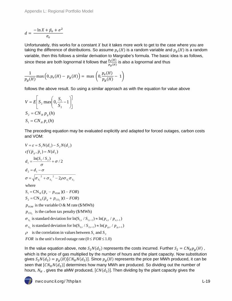
Appendix L: Regional Portfolio Model
nwcouncil.org/7thplan L-19
𝑑 = − ln𝑋 + �̅�𝑒 + 𝜎2
𝜎𝑒
Unfortunately, this works for a constant 𝑋 but it takes more work to get to the case where you are taking the difference of distributions. So assume 𝑝𝑒(𝐻) is a random variable and 𝑝𝑔(𝐻) is a random variable, then this follows a similar derivation to Margrabe’s formula. The basic idea is as follows, since these are both lognormal it follows that 𝑝𝑒(𝐻)
𝑝𝑔(𝐻) is also a lognormal and thus
1𝑝𝑔(𝐻) max �0,𝑝𝑒(𝐻) − 𝑝𝑔(𝐻)� = max �0,
𝑝𝑒(𝐻) 𝑝𝑔(𝐻) − 1�
follows the above result. So using a similar approach as with the equation for value above
)(
)(
1,0max
1
2
2
12
hpCNShpCNS
SSSEV
eH
gH
=
=
−=
The preceding equation may be evaluated explicitly and adapted for forced outages, carbon costs and VOM:
1.0)(0 rate outage forced sunit' theis and between in valuesn correlatio theis
)/ln()/ln(Sfor deviation standard is
)/ln()/ln(Sfor deviation standard is
($/MWh)penalty carbon tax theis ($/MWh) rate M&O variable theis
)1)((CN )1)((CN
where
2
2/)/ln(
)(),()()(
21
1,,1,2t2,
1,,1,1t1,
H2
H1
22
12
211
2
2211
2
1
2
2
2121
≤≤
≈
≈
−+=−−=
−+=
−=
+=
=−==
−−
−−
FORFORSS
ppS
ppS
pp
FORppSFORppS
dd
SSd
dNppcfdNSdNSV
tgtgtS
tetetS
CO
VOM
COg
VOMe
SSSS
eg
ρ
σ
σ
σρσσσσ
σ
σσ
ε
In the value equation above, note 𝑆2𝑁(𝑑2) represents the costs incurred. Further 𝑆2 = 𝐶𝑁𝐻𝑝𝑔(𝐻) , which is the price of gas multiplied by the number of hours and the plant capacity. Now substitution gives 𝑆2𝑁(𝑑2) = 𝑝𝑔(𝐻)[𝐶𝑁𝐻𝑁(𝑑2)]. Since 𝑝𝑔(𝐻) represents the price per MWh produced, it can be seen that [𝐶𝑁𝐻𝑁(𝑑2)] determines how many MWh are produced. So dividing out the number of hours, 𝑁𝐻 , gives the aMW produced, [𝐶𝑁(𝑑2)]. Then dividing by the plant capacity gives the
Appendix L: Regional Portfolio Model
nwcouncil.org/7thplan L-20
capacity factor, 𝑁(𝑑2)9. This shows that the plant dispatch can be derived from this formulation of the value of generation.
5.2 Market Balancing The previous section gives the dispatch of a thermal resource in terms of a fixed market price. However, the internal market price in the model can change and thus the dispatch would be changed. The RPM sets limits on the ability to import energy into and export energy out of the region.
If the market price from the risk model detailed above results in a dispatch that falls within this range, then there is no further alteration of the market price and the import or export of energy is determined by taking the difference between the energy produced based on the thermal dispatch and hydro dispatch and the load net of conservation and must run resources.10
If the market price from the risk model detailed above results in a dispatch that is outside this range then the price is changed and the dispatch is recalculated. When the dispatch and the import limit fall short of the net load, then the price is changed to take an average of the market price and the upper bound of the electricity price range, 325 dollars in 2012 dollars for the Seventh Plan. When the dispatch minus the export limit exceeds the net load then the price is changed to take an average of the market price and the lower bound of the electricity price range, 0 dollars in 2012 dollars for the Seventh Plan. If this change in the market price is not sufficient to result in a dispatch that falls within the range then the process is repeated. If after 12 iterations the dispatch still fails to fall within this range then penalties are assessed for Loss of Load or Oversupply.
6 OPTIMIZATION OF RESOURCE STRATEGIES The first part of understanding the optimization of resource strategies is to understand the size of the sample space. There are two adders for lost opportunity and discretionary conservation. In the many scenarios evaluated, these adders were restricted to a range of 0 to 150 dollars per megawatt-hour. Since these are both continuous variables, the resulting sample space is infinite because of just these values. However, continuous variables are well suited for optimization so these variables are easily handled.
Discrete variables are much more difficult to optimize because they can have non-smooth or jumpy impacts on the objective function, which in the case of RPM is the minimization of system cost. In most of the scenarios evaluated for the Seventh Plan, in the RPM there are more than 1.66 ∗ 10173 possible combinations of the discrete variables in the resource strategy. Even if you could run a
9 An alternate way to explain this is in terms of option theory and that the cost represents a strike price at which expectation is positive. This comes from refactoring the Black-Scholes framework for the value of an option if there was no time lag between the purchase and sale, i.e. arbitrage. 10Certain thermal, wind and solar resources are considered must-run in the RPM.

Appendix L: Regional Portfolio Model
nwcouncil.org/7thplan L-21
billion resource strategies per second it would be impossible to explore every possible combination. With the RPM setup for the Seventh Plan, it generally takes from 20 seconds to just under a minute to run through the calculations for one resource strategy. Distributed processing is used in the RPM to make these calculations in parallel. Even with distributed processing, the most combinations of potential resource strategies run for any scenario would be around 10,000. More commonly, 3,000 to 4,000 resource strategies were tested. This is an infinitesimal fraction of a percent of the possible resource strategies. To reduce the sample space investigated by the RPM, the RPM optimization is given a reasonable starting point and must look in a local region to find improvements on that starting point.
The RPM has several different algorithmic approaches available to carry out the optimization process. The most effective algorithms are what are called evolutionary algorithms. In these algorithms, a set of points in the sample space close to the starting point are taken and the results are examined at each point. The points that minimize the objective function are given more influence in selecting a new set of points in the same region. On occasion, points outside the region are added in to see if the best answer lies outside the range being examined. After a certain amount of time that is either fixed by the modeler or some amount of time that shows no improvement, the search is ended and the result that has the lowest value for the objective function is reported. The advantage of this approach is that it quickly discards strategies that are extremely expensive, usually a result of heavy penalties. The engine used for the RPM was an optimizer from Frontline11 using an Evolutionary algorithm for a Non-Smooth Problem. In general, the optimizer was able to improve on the starting point and thus moved in an optimal direction.
Because of the complexity of the problem, it is impossible to ever verify that a result is the absolute optimal resource strategy. Thus it is important to not only use the optimization routine but to also use expert (human) judgment as to the reasonableness of the results. The model can test any change to a resource strategy, whether made automatically through an algorithm or manually through exploration. To the extent possible both approaches were used and results were examined critically. While it is possible under any scenario that more optimal results could be yet undiscovered, it is unlikely that these results would significantly alter the understanding or narratives developed based on the results that were used for this plan.
6.1 Objective Function The RPM was setup with the capability to minimize the expected system cost or the tail risk, usually the TailVar90 or the average of the top 10 percent of the 800 simulated system costs. In several scenarios, the model was run to minimize on tail risk and the resulting resource strategy was compared to the resource strategy that resulted from minimizing expected system cost. In every case examined, there was not a substantive difference between these methods of optimization. That is likely because of the implementation of penalties for resource strategies that did not meet adequacy standards.
11 http://www.solver.com/

Appendix L: Regional Portfolio Model
nwcouncil.org/7thplan L-22
For the Seventh Plan, a penalty was added for resource strategies that did not meet adequacy constraints. Because a price penalty was used to enforce the adequacy constraints, all resource strategies that minimized costs contain a level of risk mitigation. If the cost and risk of the system were considered outside of these constraints, then there would likely be much more contrast between resource strategies minimizing risk and resource strategies minimizing cost.
Given these adequacy constraints, the cost and risk trade-offs were minimal at best. That is likely because the “cost of risk” is internalized in the adequacy price penalty. Thus, minimizing the system costs using the objective function incorporates a substantial amount of inherent risk mitigation.
7 REPORTING OUTPUTS The RPM has many variables that are calculated for each simulation. The main output is the system cost. There are many other outputs that can be reported. This section discusses some of the significant outputs used for communicating the results of the scenarios run in the RPM.
7.1 System Cost The system cost is based on taking a stream of costs associated with running existing generation and the costs associated with building and running new generation. The difficultly is to appropriately value conservation under this scheme. To do this the calculation is based on the frozen efficiency load and the value of reducing the load is credited to the conservation.
The main objective function in the RPM is to minimize the system cost. However, the market price impacts many components of the portfolio cost. In general, when a resource that is constructed to serve regional load is dispatched to serve regional load, the cost to the region is based on the fixed and variable cost of that resource. When a resource is dispatched to export to the market, the system cost is reduced by the difference between the variable cost of dispatching the resource and the compensation from the market. When regional load is served by the market then the cost of purchasing power at the market price is added to the system cost.
Formulating a system cost function or objective function to generalize all these potential situations is necessary to simplify the optimization. The goal is to calculate the system cost for each time and future, that is 𝑉𝑖,𝑡 = 𝑁𝑒𝑡 𝑠𝑦𝑠𝑡𝑒𝑚 𝑐𝑜𝑠𝑡 𝑎𝑡 𝑡𝑖𝑚𝑒 𝑡 𝑓𝑜𝑟 𝑓𝑢𝑡𝑢𝑟𝑒 𝑖.
First the cost of serving the load must be considered. If the load was all served at market price then it would be:
�𝐷𝑊𝑁,𝑂𝑛(𝑡, 𝑖) ∗ 𝑀𝑊𝑒𝑠𝑡,𝑂𝑛(𝑡, 𝑖) ∗ 𝐻𝑟𝑠𝑂𝑛 + 𝐷𝑊𝑁,𝑂𝑓𝑓(𝑡, 𝑖) ∗ 𝑀𝑊𝑒𝑠𝑡,𝑂𝑓𝑓(𝑡, 𝑖) ∗ 𝐻𝑟𝑠𝑂𝑓𝑓� ∗ 𝐶𝑜𝑟𝑟
Where 𝐷𝑊𝑁 is the load for on and off-peak, 𝑀𝑊𝑒𝑠𝑡 is the market price for the western side of the region, 𝐻𝑟𝑠 represents the number of hours in the on-peak and off-peak periods and 𝐶𝑜𝑟𝑟 is an adjustment factor to represents intra-period correlation between the market price and the load.
Of course when conservation is developed, then the cost of acquisition is added to the system cost but the cost of serving load at market price or at the variable cost of a resource would be reduced. That is
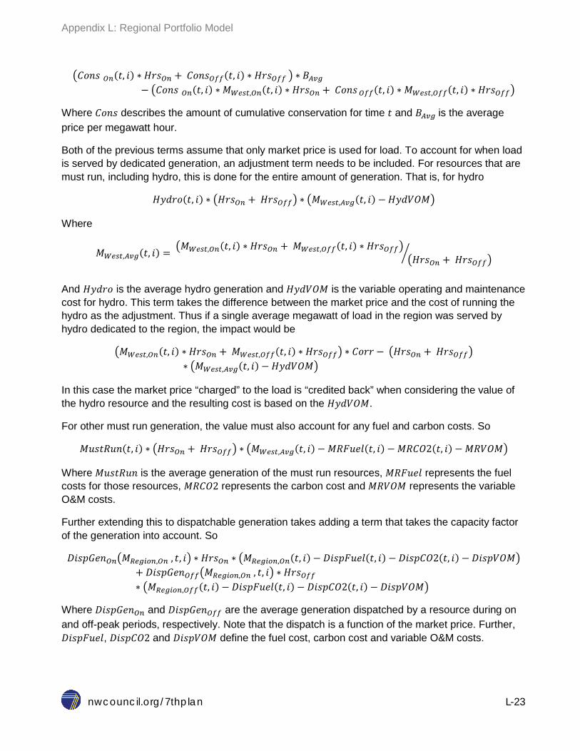
Appendix L: Regional Portfolio Model
nwcouncil.org/7thplan L-23
�𝐶𝑜𝑛𝑠 𝑂𝑛(𝑡, 𝑖) ∗ 𝐻𝑟𝑠𝑂𝑛 + 𝐶𝑜𝑛𝑠𝑂𝑓𝑓(𝑡, 𝑖) ∗ 𝐻𝑟𝑠𝑂𝑓𝑓 � ∗ 𝐵𝐴𝑣𝑔− �𝐶𝑜𝑛𝑠 𝑂𝑛(𝑡, 𝑖) ∗ 𝑀𝑊𝑒𝑠𝑡,𝑂𝑛(𝑡, 𝑖) ∗ 𝐻𝑟𝑠𝑂𝑛 + 𝐶𝑜𝑛𝑠 𝑂𝑓𝑓(𝑡, 𝑖) ∗ 𝑀𝑊𝑒𝑠𝑡,𝑂𝑓𝑓(𝑡, 𝑖) ∗ 𝐻𝑟𝑠𝑂𝑓𝑓�
Where 𝐶𝑜𝑛𝑠 describes the amount of cumulative conservation for time 𝑡 and 𝐵𝐴𝑣𝑔 is the average price per megawatt hour.
Both of the previous terms assume that only market price is used for load. To account for when load is served by dedicated generation, an adjustment term needs to be included. For resources that are must run, including hydro, this is done for the entire amount of generation. That is, for hydro
𝐻𝑦𝑑𝑟𝑜(𝑡, 𝑖) ∗ �𝐻𝑟𝑠𝑂𝑛 + 𝐻𝑟𝑠𝑂𝑓𝑓� ∗ �𝑀𝑊𝑒𝑠𝑡,𝐴𝑣𝑔(𝑡, 𝑖) −𝐻𝑦𝑑𝑉𝑂𝑀�
Where
𝑀𝑊𝑒𝑠𝑡,𝐴𝑣𝑔(𝑡, 𝑖) = �𝑀𝑊𝑒𝑠𝑡,𝑂𝑛(𝑡, 𝑖) ∗ 𝐻𝑟𝑠𝑂𝑛 + 𝑀𝑊𝑒𝑠𝑡,𝑂𝑓𝑓(𝑡, 𝑖) ∗ 𝐻𝑟𝑠𝑂𝑓𝑓��𝐻𝑟𝑠𝑂𝑛 + 𝐻𝑟𝑠𝑂𝑓𝑓��
And 𝐻𝑦𝑑𝑟𝑜 is the average hydro generation and 𝐻𝑦𝑑𝑉𝑂𝑀 is the variable operating and maintenance cost for hydro. This term takes the difference between the market price and the cost of running the hydro as the adjustment. Thus if a single average megawatt of load in the region was served by hydro dedicated to the region, the impact would be
�𝑀𝑊𝑒𝑠𝑡,𝑂𝑛(𝑡, 𝑖) ∗ 𝐻𝑟𝑠𝑂𝑛 + 𝑀𝑊𝑒𝑠𝑡,𝑂𝑓𝑓(𝑡, 𝑖) ∗ 𝐻𝑟𝑠𝑂𝑓𝑓� ∗ 𝐶𝑜𝑟𝑟 − �𝐻𝑟𝑠𝑂𝑛 + 𝐻𝑟𝑠𝑂𝑓𝑓�∗ �𝑀𝑊𝑒𝑠𝑡,𝐴𝑣𝑔(𝑡, 𝑖) −𝐻𝑦𝑑𝑉𝑂𝑀�
In this case the market price “charged” to the load is “credited back” when considering the value of the hydro resource and the resulting cost is based on the 𝐻𝑦𝑑𝑉𝑂𝑀.
For other must run generation, the value must also account for any fuel and carbon costs. So
𝑀𝑢𝑠𝑡𝑅𝑢𝑛(𝑡, 𝑖) ∗ �𝐻𝑟𝑠𝑂𝑛 + 𝐻𝑟𝑠𝑂𝑓𝑓� ∗ �𝑀𝑊𝑒𝑠𝑡,𝐴𝑣𝑔(𝑡, 𝑖) −𝑀𝑅𝐹𝑢𝑒𝑙(𝑡, 𝑖) −𝑀𝑅𝐶𝑂2(𝑡, 𝑖) −𝑀𝑅𝑉𝑂𝑀�
Where 𝑀𝑢𝑠𝑡𝑅𝑢𝑛 is the average generation of the must run resources, 𝑀𝑅𝐹𝑢𝑒𝑙 represents the fuel costs for those resources, 𝑀𝑅𝐶𝑂2 represents the carbon cost and 𝑀𝑅𝑉𝑂𝑀 represents the variable O&M costs.
Further extending this to dispatchable generation takes adding a term that takes the capacity factor of the generation into account. So
𝐷𝑖𝑠𝑝𝐺𝑒𝑛𝑂𝑛�𝑀𝑅𝑒𝑔𝑖𝑜𝑛,𝑂𝑛 , 𝑡, 𝑖� ∗ 𝐻𝑟𝑠𝑂𝑛 ∗ �𝑀𝑅𝑒𝑔𝑖𝑜𝑛,𝑂𝑛(𝑡, 𝑖) − 𝐷𝑖𝑠𝑝𝐹𝑢𝑒𝑙(𝑡, 𝑖) − 𝐷𝑖𝑠𝑝𝐶𝑂2(𝑡, 𝑖) − 𝐷𝑖𝑠𝑝𝑉𝑂𝑀�+ 𝐷𝑖𝑠𝑝𝐺𝑒𝑛𝑂𝑓𝑓�𝑀𝑅𝑒𝑔𝑖𝑜𝑛,𝑂𝑛 , 𝑡, 𝑖� ∗ 𝐻𝑟𝑠𝑂𝑓𝑓∗ �𝑀𝑅𝑒𝑔𝑖𝑜𝑛,𝑂𝑓𝑓(𝑡, 𝑖) − 𝐷𝑖𝑠𝑝𝐹𝑢𝑒𝑙(𝑡, 𝑖) − 𝐷𝑖𝑠𝑝𝐶𝑂2(𝑡, 𝑖) − 𝐷𝑖𝑠𝑝𝑉𝑂𝑀�
Where 𝐷𝑖𝑠𝑝𝐺𝑒𝑛𝑂𝑛 and 𝐷𝑖𝑠𝑝𝐺𝑒𝑛𝑂𝑓𝑓 are the average generation dispatched by a resource during on and off-peak periods, respectively. Note that the dispatch is a function of the market price. Further, 𝐷𝑖𝑠𝑝𝐹𝑢𝑒𝑙, 𝐷𝑖𝑠𝑝𝐶𝑂2 and 𝐷𝑖𝑠𝑝𝑉𝑂𝑀 define the fuel cost, carbon cost and variable O&M costs.

Appendix L: Regional Portfolio Model
nwcouncil.org/7thplan L-24
This does not account for the fixed costs of adding generation to the system. The planning, construction and the fixed O&M costs must be added into the system costs. These costs differ by resource and thus are a function of the resource:
𝐷𝑖𝑠𝑝𝑃𝑙𝑎𝑛(𝑅𝑒𝑠𝑜𝑢𝑟𝑐𝑒, 𝑡, 𝑖) + 𝐷𝑖𝑠𝑝𝐶𝑜𝑛𝑠𝑡𝑟(𝑅𝑒𝑠𝑜𝑢𝑟𝑐𝑒, 𝑡, 𝑖) + 𝐷𝑖𝑠𝑝𝐹𝑂𝑀(𝑅𝑒𝑠𝑜𝑢𝑟𝑐𝑒, 𝑡, 𝑖)
Where 𝐷𝑖𝑠𝑝𝑃𝑙𝑎𝑛, 𝐷𝑖𝑠𝑝𝐶𝑜𝑛𝑠𝑡𝑟 and 𝐷𝑖𝑠𝑝𝐹𝑂𝑀 represent the planning, construction and fixed O&M costs for each 𝑅𝑒𝑠𝑜𝑢𝑟𝑐𝑒.
For reporting out of the RPM all these costs are added up to reach the net system cost, 𝑉𝑡,𝑖.
Note that the optimization routine uses two other components of the system cost: the costs of not being able to balance the market and the costs of not meeting adequacy standards. These penalties help the optimization find resource strategies that avoid market imbalance and inadequate systems. However, these penalty costs are not reported in the net system cost.
7.2 Net Present Value of System Costs Since the system costs represent a time stream of cash flows, these can be discounted to get a present value of system costs. This uses the standard formulation of net present value or NPV. That is for the net system cost 𝑉𝑡,𝑖 the net present value for future 𝑖 is
𝑁𝑃𝑉𝑆𝑡𝑢𝑑𝑦,𝑖 = �𝑉𝑡,𝑖
(1 + 𝑑𝑖𝑠𝑐)𝑡80
𝑡=1
Where 𝑑𝑖𝑠𝑐 is the discount rate for the calculation and 𝑁𝑃𝑉𝑆𝑡𝑢𝑑𝑦 represents the value of the study horizon, i.e. 𝑡 = 1 𝑡𝑜 80.
7.2.1 Perpetuity Effects
The value within the study horizon does not account for the impacts of the resource strategy that carry beyond the scope of the study. The RPM estimates these effects using calculations based on the NPV formulation. To estimate these effects there needs to be an estimate for the system cost after time 𝑡 = 80. For the Seventh Plan, the last eight periods were used to estimate the impacts to system cost going into perpetuity. That is, the estimate of for 𝑉𝑡=81,𝑖 = 𝑉𝑡=73,𝑖 or more generally, 𝑉𝑡,𝑖 = 𝑉𝑡−8,𝑖 𝑓𝑜𝑟 𝑎𝑙𝑙 𝑡 > 80. Given this estimate, the NPV can be considered over an infinite time period, that is
𝑁𝑃𝑉𝑖 = 𝑁𝑃𝑉𝑆𝑡𝑢𝑑𝑦,𝑖 + 𝑁𝑃𝑉𝑃𝑒𝑟𝑝,𝑖 = �𝑉𝑡,𝑖
(1 + 𝑑𝑖𝑠𝑐)𝑡80
𝑡=1+ �
𝑉𝑡,𝑖(1 + 𝑑𝑖𝑠𝑐)𝑡
∞
𝑡=81
Now for 𝑡 > 80,
𝑉𝑡,𝑖 = 𝑉𝑡−8,𝑖
So
1(1 + 𝑑𝑖𝑠𝑐)𝑡 𝑉𝑡,𝑖 =
1(1 + 𝑑𝑖𝑠𝑐)𝑡 𝑉𝑡−8,𝑖 =
1(1 + 𝑑𝑖𝑠𝑐)8 �
1(1 + 𝑑𝑖𝑠𝑐)𝑡−8 𝑉𝑡−8,𝑖�

Appendix L: Regional Portfolio Model
nwcouncil.org/7thplan L-25
This allows the perpetuity equation to be rearranged to
𝑁𝑃𝑉𝑃𝑒𝑟𝑝,𝑖 = � ��1
(1 + 𝑑𝑖𝑠𝑐)8𝑗∞
𝑗=1� 𝑉𝑡,𝑖
80
𝑡=73= ��
1(1 + 𝑑𝑖𝑠𝑐)8𝑗
∞
𝑗=1�� 𝑉𝑡,𝑖
80
𝑡=73
Now it turns out that �∑ 1(1+𝑑𝑖𝑠𝑐)8𝑗
∞𝑗=1 � is a geometric series12 and 1
(1+𝑑𝑖𝑠𝑐)8 < 1, so
��1
(1 + 𝑑𝑖𝑠𝑐)8𝑗∞
𝑗=1�� 𝑉𝑡,𝑖
80
𝑡=73=
11 − (1 + 𝑑𝑖𝑠𝑐)−8� 𝑉𝑡,𝑖
80
𝑡=73
Thus
𝑁𝑃𝑉𝑖 = �𝑉𝑡,𝑖
(1 + 𝑑𝑖𝑠𝑐)𝑡80
𝑡=1+
11 − (1 + 𝑑𝑖𝑠𝑐)−8� 𝑉𝑡,𝑖
80
𝑡=73
7.3 Carbon Emissions The dispatch, detailed earlier in this chapter, determines the amount of carbon emissions from resources that emit carbon that are both in the region and those that are out of region but are contracted to serve the region. Also, the emissions related to imports not related to the resources in RPM are added to the regional emissions. Imports are assigned a carbon dioxide emission rate of around half a metric ton per megawatt hour.
Note, separating the regional emissions from the WECC-wide emissions may give a false impression of the impact of a scenario. There may be scenarios that would result in higher regional emissions but result in lower WECC-wide emissions, as well as scenarios that result in lower regional emissions but would result in higher WECC-wide emissions. When considering carbon emissions from the RPM, the imports and exports from the region should be considered carefully as part of the resulting narrative. This phenomenon likely impacts scenarios with the largest carbon reductions more than other scenarios.
The RPM also has an estimate of the emissions related to the Environmental Protection Agency’s Clean Power Plan (CPP). This is calculated by taking a subset of the plants in the region and estimating those emissions. Since the CPP includes only carbon dioxide emissions within state boundaries, imports are not counted in this calculation.
12The convergence of a geometric series shows that ∑ 𝑥𝑖∞
𝑖=0 = 1 + 𝑥 + 𝑥2 + 𝑥3 + … = 1(1−𝑥) 𝑓𝑜𝑟 0 < 𝑥 < 1

Seventh Northwest Conservation and Electric Power Plan
nwcouncil.org/7thplan M-1
APPENDIX M: CLIMATE CHANGE IMPACTS TO LOADS AND RESOURCES
Contents Key Findings ..................................................................................................................................... 3 Background ....................................................................................................................................... 4 Temperature and Hydrological Changes ........................................................................................... 6
Precipitation, Snow Pack, and River Flows .................................................................................... 8 Electricity Demand ......................................................................................................................... 9
Impacts to the Power System .......................................................................................................... 17 Methodology ................................................................................................................................ 17 Assumptions ................................................................................................................................ 18 Regulated Flows and Hydroelectric Generation ........................................................................... 25 Reservoir Storage ........................................................................................................................ 27 Power Supply Adequacy .............................................................................................................. 28 Climate Change Effects on the Seventh Plan............................................................................... 30
Other Climate Change Impacts ....................................................................................................... 30 Modeling Climate Change in the Regional Portfolio Model .............................................................. 32 Conclusions and Recommendations ............................................................................................... 34

Appendix M: Climate Change Impacts to Loads and Resources
nwcouncil.org/7thplan M-2
List of Figures and Tables
Figure M - 1: Average vs. Year-to-Year Variation in the 80-Year River-Flow Data Set ..................... 6 Figure M - 2: Columbia Basin Temperature and Precipitation Change Forecasts ............................. 7 Figure M - 3a: Average Unregulated Flows at The Dalles Historic vs. 2045 Climate Change .......... 8 Figure M - 4a: 2045 Climate Induced Change in Unregulated Flows at The Dalles .......................... 9 Figure M - 5: Illustration of Projected Temperature Increase (2015 to 2035) .................................. 10 Figure M - 6: 2035 Climate Induced Monthly Temperature Changes ............................................. 11 Table M - 1: Cooling/Heating Degree Days by State ...................................................................... 11 Figure M - 7: Increased Air-conditioning Penetration Rates (Residential) ....................................... 12 Figure M - 8: Change in Peak and Energy Loads for a 4.3° F Annual Increase in Temperature .... 13 Figure M - 9: Peak Load Forecast under a Climate Change Scenario (MW).................................... 14 Figure M - 10: Energy Load Forecast under a Climate Change Scenario (aMW) ............................ 14 Figure M - 11: IPCC 5 Report Projected Changes in Global Temperature ...................................... 15 Table M - 2: Assumed Temperature Changes using a Linear Interpolation ..................................... 16 Figure M - 12a: Projected Changes for West North America Jun-Aug ............................................ 16 Figure M - 12b: Projected Changes for West North America Dec-Feb ............................................ 17 Figure M - 3b: Average Unregulated Flows at The Dalles ............................................................... 19 Historic, 2045 Climate and Fitted Values ......................................................................................... 19 Figure M - 4b: 2045 Forecast Change in Unregulated Flows at The Dalles .................................... 19 Figure M - 13a: 2026 Projected Change in Unregulated Flows at The Dalles ................................. 20 Figure M - 13b: 2035 Projected Change in Unregulated Flows at The Dalles ................................. 21 Figure M - 14a: 2026 Projected Change in Average and Peak Loads............................................. 21 Figure M - 14b: 2035 Projected Change in Average and Peak Loads............................................. 22 Figure M - 15: Load Paths for Two Different Futures out of RPM ................................................... 23 Figure M - 16a: 2026 Projected Resource Development (RPM Future 781) ................................... 24 Figure M - 16b: 2035 Projected Resource Development (RPM Future 70) ..................................... 24 Figure M - 17: Projected Change in Regulated Flows at McNary Dam ........................................... 26 Figure M - 18: Projected Change in Hydroelectric Generation ........................................................ 26 Table M - 3: Climate Induced Impacts to Energy Load/Resource Balance (aMW) .......................... 27 Figure M - 19: Climate Induced Change in Storage (Coulee, Libby, Horse and Dworshak) ........... 28 Figure M - 20a: 2026 Projected Change in Expected Loss of Load ................................................ 29 Figure M - 20b: 2035 Projected Change in Expected Loss of Load ................................................ 29 Figure M - 21: When Additional Resources may be needed to offset Climate Change .................... 30 Figure M - 22: Illustrative Probability Distribution for Climate Model Results ................................... 33

Appendix M: Climate Change Impacts to Loads and Resources
nwcouncil.org/7thplan M-3
KEY FINDINGS There are at least two ways in which climate change can affect the power plan. First, long-term changes in temperature will alter electricity demand and change precipitation patterns, river flows and hydroelectric generation. Second, policies enacted to reduce greenhouse gases will affect future resource choices. While the Council is not tasked with nor does it have the resources to resolve these uncertainties, it does have the obligation to investigate possible impacts of climate change on the region’s power system and to recommend actions to maintain the adequacy, reliability, efficiency and economy of the system whenever appropriate. A discussion of greenhouse gas policies and their influence on resource choices is discussed in detail in Chapters 3 and 15. This appendix addresses the potential physical impacts of climate change and how they may affect the power plan.
Council analysis shows that climate induced changes to loads and river flows will not affect resource choices during the action plan period (2016 through 2021). However, beyond 2026, if load growth is higher than average, resource decisions would be different under a scenario in which climate change is considered. Because of this, the Council will continue to monitor and participate in efforts to improve climate change data and analysis, as provided by the Intergovernmental Panel on Climate Change (IPCC) and regional entities that downscale that data for Northwest use.
The most recent IPCC report1 (Assessment Report 5) indicates that future global temperatures are very likely to increase. Unfortunately, data collected from global climate modeling will not be downscaled and processed for the Northwest region until early 2017 – much too late for analysis to be included in the Seventh Power Plan. However, some of the new IPCC data can be used in combination with existing data to analyze potential physical impacts to the Northwest power system.
From previous climate modeling downscaling efforts, the prediction for the Northwest is for less snow and more rain during winter months, resulting in a smaller spring snowpack and lower summer flows.2 Winter electricity demands would decrease with warmer temperatures, easing generating requirements. In the summer, demands driven by air conditioning and irrigation loads would rise.
The power supplies for both 2026 and 2035, as projected by the Regional Portfolio Model under a future high-load path, were examined under two scenarios, one without climate change and one with projected climate change effects. Results show that the 2026 power supply meets the Council’s
1 IPCC, 2013: Annex I: Atlas of Global and Regional Climate Projections [van Oldenborgh, G.J., M. Collins, J. Arblaster, J.H. Christensen, J. Marotzke, S.B. Power, M. Rummukainen and T. Zhou (eds.)]. In: Climate Change 2013: The Physical Science Basis. Contribution of Working Group I to the Fifth Assessment Report of the Intergovernmental Panel on Climate Change [Stocker, T.F., D. Qin, G.-K. Plattner, M. Tignor, S.K. Allen, J. Boschung, A. Nauels, Y. Xia, V. Bex and P.M. Midgley (eds.)]. Cambridge University Press, Cambridge, United Kingdom and New York, NY, USA.
2 For general details and a description of projected climate change effects for the Northwest, see p. 57 in the Climate Change strategy of the Council’s 2014 Columbia River Basin Fish & Wildlife Program and Appendix G of that program.

Appendix M: Climate Change Impacts to Loads and Resources
nwcouncil.org/7thplan M-4
adequacy standard in both cases. Thus, up through 2026, no additional resources are required to maintain an adequate supply, even under a climate change scenario. The same is true in 2035 for the no climate change case. However, after applying the climate induced shift in river flows and load, the likelihood of a shortfall in 2035 grows to 15 percent, which is far above the Council’s adequacy standard of 5 percent. In this case additional resources would have to be acquired to maintain adequacy.
The Council’s analysis indicates that climate induced changes to river flows and loads will not alter resource acquisition strategies at least until 2026. Thus, in the near term, climate change effects do not render the system inadequate and do not require modification to the resource acquisitions identified over the next six years.
Other potential climate change impacts include increased flooding concerns in fall and winter, reduced salmon migration survival due to lower summer river flows combined with higher water temperatures and increased summer electricity prices.
Though the physical effects of climate change remain imperfectly understood, the Council has examined them and recommends that research continue in this area. While no immediate actions regarding reservoir operations are indicated, the region should begin to examine and consider alternative reservoir operations that could potentially mitigate for potential future climate change impacts.
BACKGROUND In 1988 the United Nations Environment Programme (UNEP) and the World Meteorological Organization (WMO) established the Intergovernmental Panel on Climate Change (IPCC), which was subsequently endorsed by the United Nations General Assembly.3 The IPCC was established to assess available scientific, technical and socio-economic information concerning climate change, its potential effects, and options for adaptation and mitigation. The IPCC’s purpose is to collect and review the most recent scientific information produced worldwide relevant to the understanding of climate change. It does not conduct any research on its own nor does it monitor climate-related data. It is open to all member countries of the United Nations and currently has 195 participating countries that review all of the scientific material to ensure an objective and complete assessment of current information.
In November of 2014 the IPCC completed its Fifth Assessment Report (AR5).4 Most participating organizations use complex computer models, commonly known as “global circulation models” or GCMs, to forecast long-term changes in the Earth’s climate. These models primarily focus on the effects of greenhouse gases on temperature and precipitation. They take into account the interaction
3See “IPCC Factsheet: Timeline – highlights of IPCC history” at http://www.ipcc.ch/news_and_events/docs/factsheets/FS_timeline.pdf. 4 See link at http://www.ipcc.ch/index.htm.

Appendix M: Climate Change Impacts to Loads and Resources
nwcouncil.org/7thplan M-5
of the atmosphere, oceans and land surfaces.5 Each of these models has been “calibrated” to some degree and crosschecked against other such models to provide greater confidence in their forecasting ability.
Scientists are confident about their projections of climate change for large-scale areas but are less confident about projections for smaller or regional-scale areas. This is largely because computer models used to forecast global climate change are still ill-equipped to simulate how things may change on smaller scales. Forecasts on a global level therefore are of little use to planners in the Northwest. A method to downscale the output from the global models to a regional level has been developed.6 The downscaled data match better with hydrological data used to simulate the operation of the Columbia River hydroelectric power system. By using forecast temperature and precipitation changes, downscaled for the Northwest, a range of climate-affected potential future river-flow conditions and temperatures can be developed. The climate-adjusted river-flow data set is used as input to the Council’s GENESYS model, which estimates impacts to hydroelectric generation, regulated river flows and reservoir elevations. Projected temperature changes lead to adjustments in electricity demand forecasts.
There are at least 20 different global circulation models that project future changes in temperature and precipitation. Every one of these models, to varying degrees, forecasts a warming trend for the Earth. Each uses modern mathematical techniques to simulate changes in temperature as a function of atmospheric and other conditions. Like all fields of scientific study, however, there are uncertainties associated with assessing the question of global warming and, as we are often reminded, a computer model is only as good as its input assumptions. The effects of weather (in particular precipitation) and ocean conditions are still not well known and are often inadequately represented in climate models – although both play a major role in determining future climate.
Generally, results from the most relevant GCM models are downscaled for the Northwest by several groups in the region, in particular the Climate Impacts Group at the University of Washington in conjunction with the River Management Joint Operating Committee (RMJOC). The downscaled data are processed to ultimately produce two components that are necessary for the Council’s analysis: 1) a set of climate-change-adjusted unregulated river flows (including an appropriate set of reservoir rule curves); and 2) a set of projected monthly and daily temperature changes for future years. As mentioned earlier, the temperature data are used to adjust future load forecasts and the river-flow data are used as input to the GENESYS model to determine the output of the region’s hydroelectric system.
Unfortunately, data from the most recent IPCC report (AR5) GCMs are still in the process of being downscaled for Northwest use and will not be available until late 2016 or early 2017. The most recent complete set of downscaled data is based on the 2007 AR4 report, which although outdated,
5 http://gcrio.org/CONSEQUENCES/fall95/mod.html
6 Wood, A.W., Leung, L. R., Sridhar, V., Lettenmaier, Dennis P., no date: “Hydrologic implications of dynamical and statistical approaches to downscaling climate model surface temperature and precipitation fields.”
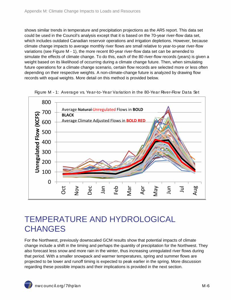
Appendix M: Climate Change Impacts to Loads and Resources
nwcouncil.org/7thplan M-6
shows similar trends in temperature and precipitation projections as the AR5 report. This data set could be used in the Council’s analysis except that it is based on the 70-year river-flow data set, which includes outdated Canadian reservoir operations and irrigation depletions. However, because climate change impacts to average monthly river flows are small relative to year-to-year river-flow variations (see Figure M - 1), the more recent 80-year river-flow data set can be amended to simulate the effects of climate change. To do this, each of the 80 river-flow records (years) is given a weight based on its likelihood of occurring during a climate change future. Then, when simulating future operations for a climate change scenario, certain flow records are selected more or less often depending on their respective weights. A non-climate-change future is analyzed by drawing flow records with equal weights. More detail on this method is provided below.
Figure M - 1: Average vs. Year-to-Year Variation in the 80-Year River-Flow Data Set
TEMPERATURE AND HYDROLOGICAL CHANGES For the Northwest, previously downscaled GCM results show that potential impacts of climate change include a shift in the timing and perhaps the quantity of precipitation for the Northwest. They also forecast less snow and more rain in the winter, thus increasing unregulated river flows during that period. With a smaller snowpack and warmer temperatures, spring and summer flows are projected to be lower and runoff timing is expected to peak earlier in the spring. More discussion regarding these possible impacts and their implications is provided in the next section.
0
100
200
300
400
500
600
700
800
Oct
Nov
Dec
Jan
Feb
Mar
Apr
May
Jun Jul
Aug
Unr
egul
ated
Flo
w (K
CFS)
Average Natural Unregulated Flows in BOLD BLACK Average Climate Adjusted Flows in BOLD RED

Appendix M: Climate Change Impacts to Loads and Resources
nwcouncil.org/7thplan M-7
Downscaled hydrologic and temperature data for the Northwest used for analysis in the Sixth Power Plan were obtained in 2009 from the Joint Institute for the Study of Atmosphere and Ocean (JISAO)7 Climate Impacts Group (CIG)8 at the University of Washington. This information, which was prepared for a single climate change scenario, was a composite of results from several climate models used by the CIG. This scenario roughly represented an “expected” or average climate change forecast.
A summary of forecasted annual temperature and precipitation changes from the downscaled AR4 data set is shown in Figure M - 2. In this figure, the X-axis represents changes from current conditions in annual precipitation (in millimeters) and the Y-axis represents changes in annual temperature (in degrees Centigrade). Each point in this figure represents the average precipitation and temperature change for each climate change scenario studied by the CIG. For example, the point labeled “3” indicates that the average annual precipitation in the 2020s is forecast to be about 0.5 millimeters greater and the average annual temperature is forecast to be about 1 degree Centigrade greater (than a non-climate change scenario). In spite of the fact that these data are old, three conclusions drawn from this figure are still relevant today; 1) each model shows a net temperature increase, 2) nothing definitive can be said about the change in total annual amount of precipitation and 3) there is great uncertainty in both the temperature and precipitation forecasts.
Figure M - 2: Columbia Basin Temperature and Precipitation Change Forecasts*
* Taken from the River Management Joint Operation Committee’s preliminary summary of the University of Washington Climate Impacts Group’s Global Climate Model analyses for the Northwest (RMJOC_Task1.2_ExploreScenariosSpread_v2.xls).
7 http://tao.atmos.washington.edu/main.html 8 http://tao.atmos.washington.edu/PNWimpacts/index.html
BASIN_WIDE
1
2
3
4
5
678
9
10
1112
13
1415
1617
18
0.00
0.20
0.40
0.60
0.80
1.00
1.20
1.40
1.60
1.80
-4.00 -3.00 -2.00 -1.00 0.00 1.00 2.00 3.00 4.00 5.00 6.00change in Precip (mm)
chan
ge in
Tem
p (°
C)
mean annual2020s

Appendix M: Climate Change Impacts to Loads and Resources
nwcouncil.org/7thplan M-8
Precipitation, Snow Pack, and River Flows Every global circulation model whose results were downscaled for the Northwest indicates that the region will become warmer across each month of the year. If this happens, less precipitation will fall as snow during fall and winter months, thus reducing the amount of snowpack in the mountains. The resulting increase in fall and winter rainfall will make unregulated river flows higher. In the spring and summer months, unregulated flows will decrease due to the smaller snowpack. The downscaled results of global models also predict that the timing of the peak spring flows for the 2040 to 2050 time period could occur as much as a month earlier, on average, than it does now. Figure M - 3a shows the average historical unregulated monthly flows for the Columbia River at The Dalles Dam along with the average unregulated flows adjusted for climate change effects for 2045. Figure M - 4a highlights these effects by plotting the change in average flows at The Dalles Dam by month.
While some of these monthly hydrologic changes are large (i.e. an average flow reduction of almost 40,000 cubic feet per second in July), they are not expected to occur until the 2040 to 2050 decade. As will be demonstrated in a later section, annual changes to temperature and consequently river flows from today through 2045 are expected to change gradually and in a non-linear fashion (with changes growing more rapidly later in the period). In fact, climate-induced changes to monthly river flows in the near-term are difficult to detect due to the large natural variance in annual weather patterns as shown in Figure M - 1.
Figure M - 3a: Average Unregulated Flows at The Dalles Historic vs. 2045 Climate Change
0
100
200
300
400
500
Oct
Nov
Dec
Jan
Feb
Mar
Apr
Ma y Jun Jul
Aug
Sep
Unr
egul
ated
Flo
w (K
CFS)
Historic CC

Appendix M: Climate Change Impacts to Loads and Resources
nwcouncil.org/7thplan M-9
Figure M - 4a: 2045 Climate Induced Change in Unregulated Flows at The Dalles
Electricity Demand There is a clear relationship between temperature and electricity demand. For electrically heated homes, as the temperature increases in winter months, electricity use goes down. In summer months, higher temperatures translate into higher demand as the use of air conditioning units rises and as a higher percentage of air conditioning units are installed. The Council uses its long-term load forecasting model to simulate the impact of increasing temperatures.
Climate-induced temperature increases are not expected to grow linearly over time. The AR4 data indicate that temperature increases should grow gradually, as illustrated in Figure M - 5. This general trend for global temperature increase was used to interpolate the projected 2045 temperature increase back to 2035. That interpolation resulted in an estimated temperature increase of 2.05 degrees Centigrade (or about 4.3 degrees Fahrenheit) by 2035. These temperature increases were used to develop a climate induced load forecast for 2035, as will be described below.
-50000
-40000
-30000
-20000
-10000
0
10000
20000
30000
40000
50000
OCT
NO
V
DEC
JAN
FEB
MAR
APR1
APR2
MAY
JUN
JUL
AUG
1
AUG
2
SEP
Flow
(cfs
)

Appendix M: Climate Change Impacts to Loads and Resources
nwcouncil.org/7thplan M-10
Figure M - 5: Illustration of Projected Temperature Increase (2015 to 2035)
Using historic heating and cooling degree days and their relationship to system peak load and system energy characteristics, the model estimates that by 2035 summer peak loads could be higher by about 3,500 megawatts and energy loads would be higher by about 1,200 average megawatts. Correspondingly, winter peak and energy loads could be lower by 120 megawatts and 70 average megawatts, respectively. Figure M - 6 shows the assumed increase in monthly temperature by 2035 used for this analysis. Just like the river-flow data set, temperature year records have a great deal of variation year to year. To simplify this analysis, only the average temperate increases over time were considered when producing the climate change revised load forecast.
It should be noted that this analysis incorporates projected increases in average regional temperature. It is likely that sub-regional warming could be more pronounced east of the Cascades, and less pronounced in the major coastal cities, which are more responsive to ocean water temperatures. However, any attempts to assess the impacts of sub-regional temperature changes over time are beyond the scope of this analysis.
0.00
1.00
2.00
3.00
0 5 10 15 20 25
Deg
rees
C
Out Years
Based on the IPCC AR4 Report (which is obsolete but illustrates the general relationship)

Appendix M: Climate Change Impacts to Loads and Resources
nwcouncil.org/7thplan M-11
Figure M - 6: 2035 Climate Induced Monthly Temperature Changes
The projected increases in annual and monthly temperatures from the AR4 downscaled data are converted to higher cooling and lower heating degree days for each state. The cooling and heating degree days are measured as the average of annual cooling or heating degree days for years 1985 through 2012. The cooling and heating degree days vary by state. For example, under normal conditions, the annual cooling degree day value for state of Idaho is about 482 degree days. In the preliminary climate change scenario, the normal cooling degree days is forecast to increase to 849 degrees by 2035. Each state’s normal and 2035 forecast cooling and heating degree day values are shown in Table M - 1 below.
Table M - 1: Cooling/Heating Degree Days by State
Cooling Degree
Days (Normal)
(1985-2012)
Cooling
Degree Days
(2035)
Heating Degree
Days (Normal)
(1985-2012)
Heating
Degree Days
(2035)
ID 482 849 6,755 5,931
MT 267 470 8,159 7,164
OR 229 403 5,171 4,540
WA 189 333 5,531 4,856
0.0
1.0
2.0
3.0
4.0
5.0
6.0
Jan Feb Mar Apr May Jun Jul Aug Sep Oct Nov Dec
Degr
ees
Change in Temperature - Degree C
Change in Temperature - Degree F

Appendix M: Climate Change Impacts to Loads and Resources
nwcouncil.org/7thplan M-12
As with all forecasts about the future, there is uncertainty regarding whether these trends will actually materialize at the pace projected. For example, the forecast growth in summer peak loads results from the assumption that due to higher summer temperatures more residential consumers will install central air conditioning. Figure M - 7 shows the assumed market shares of air conditioning across three residential housing types. Given the historical trend towards increased air conditioning, the growth in penetration shown in Figure M - 7 is not unrealistic. Nevertheless, it is still a forecast, not a fact.
Summer loads are more sensitive to temperature than winter loads. Regional variations in summer temperatures are greater than variations in winter temperatures. Figure M - 8 shows the forecasted monthly increase for energy and peak loads. Peak load is measured at the time of system peak (coincident peak).
Figure M - 7: Increased Air-conditioning Penetration Rates (Residential)
0%
10%
20%
30%
40%
50%
60%
70%
80%
2015
20
16
2017
20
18
2019
20
20
2021
20
22
2023
20
24
2025
20
26
2027
20
28
2029
20
30
2031
20
32
2033
20
34
2035
Mar
ket S
atur
atio
n
Single Family
Multi Family
Manufactured Homes
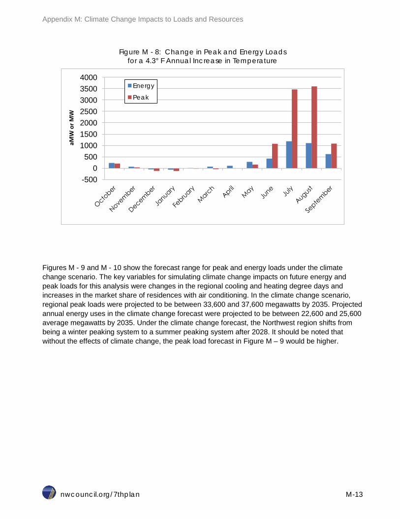
Appendix M: Climate Change Impacts to Loads and Resources
nwcouncil.org/7thplan M-13
Figure M - 8: Change in Peak and Energy Loads for a 4.3° F Annual Increase in Temperature
Figures M - 9 and M - 10 show the forecast range for peak and energy loads under the climate change scenario. The key variables for simulating climate change impacts on future energy and peak loads for this analysis were changes in the regional cooling and heating degree days and increases in the market share of residences with air conditioning. In the climate change scenario, regional peak loads were projected to be between 33,600 and 37,600 megawatts by 2035. Projected annual energy uses in the climate change forecast were projected to be between 22,600 and 25,600 average megawatts by 2035. Under the climate change forecast, the Northwest region shifts from being a winter peaking system to a summer peaking system after 2028. It should be noted that without the effects of climate change, the peak load forecast in Figure M – 9 would be higher.
-500 0
500 1000 1500 2000 2500 3000 3500 4000
aMW
or M
W
Energy
Peak

Appendix M: Climate Change Impacts to Loads and Resources
nwcouncil.org/7thplan M-14
Figure M - 9: Peak Load Forecast under a Climate Change Scenario (MW)
Figure M - 10: Energy Load Forecast under a Climate Change Scenario (aMW)
The more current AR5 data indicate that at a global level, the range of temperature increases by 2045 will be less than what was projected by the AR4 data. The current temperature projections globally and for Western North America are shown in Figures M - 11, M - 12a and M - 12b. Using the newer data, the projected average 2.05 degrees Centigrade increase by 2035 drops to an average of increase of about 0.75 degrees. On the high end of the AR5 data, the 2035 increase in average
0
5,000
10,000
15,000
20,000
25,000
30,000
35,000
40,000
1986
19
88
1990
19
92
1994
19
96
1998
20
00
2002
20
04
2006
20
08
2010
20
12
2014
20
16
2018
20
20
2022
20
24
2026
20
28
2030
20
32
2034
Syst
em P
eak
Load
(MW
)
0
5,000
10,000
15,000
20,000
25,000
30,000
1986
19
88
1990
19
92
1994
19
96
1998
20
00
2002
20
04
2006
20
08
2010
20
12
2014
20
16
2018
20
20
2022
20
24
2026
20
28
2030
20
32
2034
Syst
em A
nnua
l Loa
ds (a
MW
)

Appendix M: Climate Change Impacts to Loads and Resources
nwcouncil.org/7thplan M-15
temperature could be as much as 1.5 degrees Centigrade. Table M - 2 shows the assumptions used for climate-induced average temperature increases for 2026 and 2035. These assumptions are based on a linear relationship between projected out-year temperature increases and current temperatures. A linear relationship was assumed because insufficient information was available to extract the non-linear relationship (as illustrated in Figure M - 5). However, by using a linear relationship, the projected temperature increases are slightly higher than would be expected, thus making this analysis more pessimistic with regard to climate-induced impacts.
The climate-induced load adjustments shown in Figure M - 8 were adjusted to reflect the lower temperature increase projections from the newer AR5 data. The loads were adjusted in a linear fashion for each month. In other words, the monthly energy and peak load change for the 2.05 degree temperature increase was modified proportionally for the 0.75 and 1.5 degree increases.
Figure M - 11: IPCC 5 Report Projected Changes in Global Temperature*
* Source: “Climate Change 2013 The Physical Science Basis,” Working Group I contribution to the Fifth assessment report of the Intergovernmental Panel on Climate Change
High - 1.5 deg C Increase over 2015
Average - 0.75 deg C Increase over 2015

Appendix M: Climate Change Impacts to Loads and Resources
nwcouncil.org/7thplan M-16
Table M - 2: Assumed Temperature Changes using a Linear Interpolation
Year 2026 2035
High 0.75 °C 1.50 °C
Medium 0.38 °C 0.75 °C
Figure M - 12a: Projected Changes for West North America Jun-Aug

Appendix M: Climate Change Impacts to Loads and Resources
nwcouncil.org/7thplan M-17
Figure M - 12b: Projected Changes for West North America Dec-Feb9
IMPACTS TO THE POWER SYSTEM Methodology To assess climate change impacts, the Council uses the GENESYS computer model, which simulates the physical operation of hydroelectric and thermal resources in the Northwest. GENESYS is a Monte Carlo program that performs an economic dispatch of resources to serve regional demand. The model splits the Northwest region into eastern and western portions to capture the possible effects of cross-Cascade transmission limits. It also accounts for available out-of-region imports, if needed, to maintain continuous service to Northwest customers. Outages on the cross-Cascade and inter-regional transmission lines are not modeled.
Important future uncertainties that are explicitly modeled include unregulated river flows, temperatures (as they affect electricity loads), forced outages on thermal generating units and variability in wind generation. The model simulates the operation of the power system for a single future operating year thousands of times, with each simulation (or game) drawing randomly from the unknown parameters identified above.
9 Source: IPCC 5, Annex I: Atlas of Global and Regional Climate Projections, Figure AI.16, page 1330, Figure AI.17, page 1331

Appendix M: Climate Change Impacts to Loads and Resources
nwcouncil.org/7thplan M-18
Key outputs from the model include reservoir elevations, regulated river flows and hydroelectric system generation. The model also tracks reserve margin violations and service curtailments and assesses the adequacy of the power supply.
Assumptions The most direct way of assessing the impact to the power system of changes in unregulated river flow is to simply replace the current set with a set that has been adjusted for climate change. Unfortunately, climate-adjusted unregulated flow data sets will not be available until late 2016 or early 2017. Thus, because the AR5 data have not yet been downscaled for the region and converted into a useable form for GENESYS, an alternative approach was taken to approximate what the climate-adjusted unregulated flows would be.
Because annual variations in unregulated flows are so wide (see Figure M - 1) relative to the average change due to climate effects, it seems likely that many of the historical river flow conditions would also appear in a climate change future. To determine which ones and how often they may appear, an optimization program was used to assign a specific weight to each of the 80 river-flow records. Then, when flow records are drawn at random based on their individual weights enough times (i.e. the larger the weight, the more likely that record will be chosen), the resulting average monthly unregulated flows should closely match the projected average changes from the AR5 data. For this analysis, 6,000 simulations were performed, drawing randomly from the weighted set of 80 flow records, of which only 12 had weights significantly larger than zero. Figures M - 3b and M - 4b are identical to Figures M - 3a and M - 4a, with the addition of the optimally fitted curves that approximate the average climate change flows.

Appendix M: Climate Change Impacts to Loads and Resources
nwcouncil.org/7thplan M-19
Figure M - 3b: Average Unregulated Flows at The Dalles
Historic, 2045 Climate and Fitted Values
Figure M - 4b: 2045 Forecast Change in Unregulated Flows at The Dalles
0
100
200
300
400
500
OCT
NO
V
DEC
JAN
FEB
MAR
APR1
APR2
MAY
JUN
JUL
AUG1
AUG2
SEP
Unr
egul
ated
Flo
w (K
cfs)
Historic CC Flows
-50000
-40000
-30000
-20000
-10000
0
10000
20000
30000
40000
50000
OCT
NO
V
DEC
JAN
FEB
MAR
APR1
APR2
MAY
JUN
JUL
AUG
1
AUG
2
SEP
Flow
(cfs
)
CC Delta from HADGEM1 Study Fit Delta using 2045 Water Year Weights
CC Delta Fit Delta
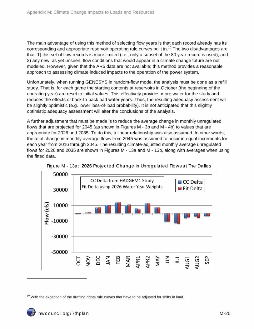
Appendix M: Climate Change Impacts to Loads and Resources
nwcouncil.org/7thplan M-20
The main advantage of using this method of selecting flow years is that each record already has its corresponding and appropriate reservoir operating rule curves built in.10 The two disadvantages are that: 1) this set of flow records is more limited (i.e., only a subset of the 80 year record is used); and 2) any new, as yet unseen, flow conditions that would appear in a climate change future are not modeled. However, given that the AR5 data are not available; this method provides a reasonable approach to assessing climate induced impacts to the operation of the power system.
Unfortunately, when running GENESYS in random-flow mode, the analysis must be done as a refill study. That is, for each game the starting contents at reservoirs in October (the beginning of the operating year) are reset to initial values. This effectively provides more water for the study and reduces the effects of back-to-back bad water years. Thus, the resulting adequacy assessment will be slightly optimistic (e.g. lower loss-of-load probability). It is not anticipated that this slightly optimistic adequacy assessment will alter the conclusions of the analysis.
A further adjustment that must be made is to reduce the average change in monthly unregulated flows that are projected for 2045 (as shown in Figures M - 3b and M - 4b) to values that are appropriate for 2026 and 2035. To do this, a linear relationship was also assumed. In other words, the total change in monthly average flows from 2045 was assumed to occur in equal increments for each year from 2016 through 2045. The resulting climate-adjusted monthly average unregulated flows for 2026 and 2035 are shown in Figures M - 13a and M - 13b, along with averages when using the fitted data.
Figure M - 13a: 2026 Projected Change in Unregulated Flows at The Dalles
10 With the exception of the drafting rights rule curves that have to be adjusted for shifts in load.
-50000
-30000
-10000
10000
30000
50000
OCT
NO
V
DEC
JAN
FEB
MAR
APR1
APR2
MAY
JUN
JUL
AUG
1
AUG
2
SEP
Flow
(cfs
)
CC Delta from HADGEM1 Study Fit Delta using 2026 Water Year Weights
CC Delta Fit Delta
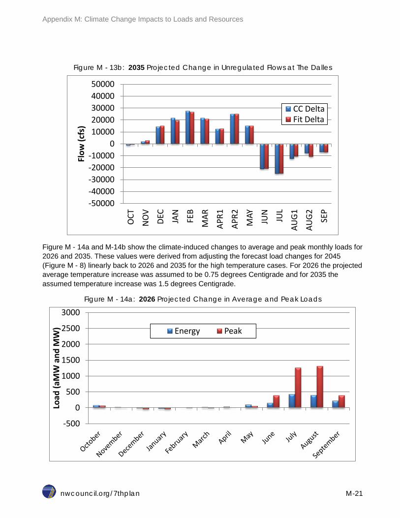
Appendix M: Climate Change Impacts to Loads and Resources
nwcouncil.org/7thplan M-21
Figure M - 13b: 2035 Projected Change in Unregulated Flows at The Dalles
Figure M - 14a and M-14b show the climate-induced changes to average and peak monthly loads for 2026 and 2035. These values were derived from adjusting the forecast load changes for 2045 (Figure M - 8) linearly back to 2026 and 2035 for the high temperature cases. For 2026 the projected average temperature increase was assumed to be 0.75 degrees Centigrade and for 2035 the assumed temperature increase was 1.5 degrees Centigrade.
Figure M - 14a: 2026 Projected Change in Average and Peak Loads
-50000 -40000 -30000 -20000 -10000
0 10000 20000 30000 40000 50000
OCT
NO
V
DEC
JAN
FEB
MAR
APR1
APR2
MAY
JUN
JUL
AUG
1
AUG
2
SEP
Flow
(cfs
)
CC Delta Fit Delta
-500
0
500
1000
1500
2000
2500
3000
Load
(aM
W a
nd M
W) Energy Peak

Appendix M: Climate Change Impacts to Loads and Resources
nwcouncil.org/7thplan M-22
Figure M - 14b: 2035 Projected Change in Average and Peak Loads
The resulting projected load changes were applied to the base load forecasts extracted from the Regional Portfolio Model simulations (futures) 781 and 70. Those specific futures generally reflect a high load growth path, which is shown in Figure M - 15. The corresponding resource acquisitions (including new energy efficiency measures) for both of these futures are shown in Figures M - 16a and M - 16b. The GENESYS model was run for both a climate-change and a non-climate-change scenario for both the 2026 and 2035 cases. The non-climate-change scenarios included the resource build out from the RPM futures and their base load forecasts. The climate-change scenario included the climate modified river-flow record and the climate modified loads – everything else was kept the same, including the resource acquisitions.
Figure M - 15 shows the Council’s low and high annual energy load forecasts for the 20-year study horizon (solid black and red curves). It also shows the particular 20-year load path from RPM futures 781 and 70, both of which show high load growth. In fact, the loads in future 781 actually slightly exceed the Council’s forecast load range. The dots on Figure M - 15 represent the operating years that were analyzed with the GENESYS model. The red dot represents the load used for 2026 and the black dot reflects the load used for 2035. Figures M - 16a and M - 16b provide the RPM produced resource build outs for these two futures. The determination of the types and amounts of new resources is guided by the logic built into the RPM but also note that these resource build outs are for two different time periods. For example, future 781, which was used to assess 2026, shows 3,380 average megawatts of energy efficiency savings. Future 70, which was used to assess 2035, develops 4,167 average megawatts of savings. Since the year studied in future 70 comes nine years after the year studied for future 781, the difference in the amount of energy efficiency developed is
-500
0
500
1000
1500
2000
2500
3000
Load
(aM
W a
nd M
W) Energy Peak

Appendix M: Climate Change Impacts to Loads and Resources
nwcouncil.org/7thplan M-23
primarily driven by these additional years, but also affected by other differences between these futures, such as natural gas and wholesale electricity prices.
The resource builds and the associated load forecasts were used in GENESYS to assess the non-climate-change scenario adequacy for 2026 and 2035. In each case, the resulting loss-of-load probability (LOLP) remained under 5 percent (the Council’s maximum threshold). Next, these two scenarios were amended to include climate change induced load changes and river flows. The results of the analyses are described in the sections below.
Figure M - 15: Load Paths for Two Different Futures out of RPM
20,000
22,000
24,000
26,000
28,000
30,000
32,000
0 5 10 15 20 Annu
al Lo
ad (A
vera
ge M
egaw
atts
)
Study Horizon Year
2035 2026 Game 70 Game 781 Low Fcst High Fcst

Appendix M: Climate Change Impacts to Loads and Resources
nwcouncil.org/7thplan M-24
Figure M - 16a: 2026 Projected Resource Development (RPM Future 781)
Figure M - 16b: 2035 Projected Resource Development (RPM Future 70)
-
500
1,000
1,500
2,000
2,500
3,000
DR CCCT SCCT Solar Wind
Inst
alle
d M
egaw
atts
Includes 3,380 Average Megawatts of EE Energy Savings
-
500
1,000
1,500
2,000
2,500
3,000
DR CCCT SCCT Solar Wind
Inst
alle
d M
egaw
atts
Includes 4,167 Average Megawatts of EE Energy Savings

Appendix M: Climate Change Impacts to Loads and Resources
nwcouncil.org/7thplan M-25
Regulated Flows and Hydroelectric Generation More rain in winter months means higher river flows at a time when electricity demand is highest in the Northwest. This, in combination with the fact that demand for electricity is likely to decrease due to warmer temperatures, should ease the pressure on the hydroelectric system to meet electricity needs in winter months. In fact, excess flow (water than cannot be stored) may be used to generate electricity that will displace higher-cost thermal resources or may be sold to out-of-region buyers.
While the future winter outlook under climate change appears to be better from a power system perspective, a more serious look at flood control operations is warranted. Some global circulation models indicate not only more fall and winter precipitation but also a higher possibility of extreme weather events, including heavy rain. This, together with warmer temperatures, should prompt the Corps of Engineers to reexamine flood risk management and the amount of its flood control releases from storage during the fall and winter period. Evacuation of water stored for flood control purposes would also add to hydroelectric generation and could further reduce the need for thermal generation during that time.
However, any winter power benefits are offset by potentially worse summer problems. With a smaller snowpack, the spring runoff volume will be correspondingly less, translating into lower river flows. On the demand side, except for the eastern portions of the Northwest, the region experiences its highest load during winter months. However, as summer temperatures increase so will electricity load due to anticipated increases in air-conditioning use. The projected increase in Northwest summer demand along with potential reductions in hydroelectric generation will force the Northwest to consider resource options for summer needs sooner rather than later.
Figure M - 17 shows the expected average regulated flow changes in 2026 and 2035 at McNary Dam due to climate impacts, which are similar to the pattern of unregulated flows shown in Figure M - 13 for The Dalles Dam.11 The difference in summer regulated flows between the climate-change scenario and the non-climate-change scenario is small when compared to the difference in summer unregulated flows. This is because additional water is released in summer for both power and fish needs (see Figure M19 for storage content changes).
Hydroelectric generation is proportional to river flow, thus it is no surprise that the average change in hydroelectric generation for 2026 and 2035 (as shown in Figure M - 18) has the same monthly shape as the change in regulated flows. Table M - 3 summarizes the changes to winter and summer loads and the respective shifts in hydroelectric generation. The data in that table highlight the observation that under a climate change future, the winter power situation is improved while the summer situation gets much worse.
11 Regulated flows at McNary Dam are shown here because the Council’s Fish and Wildlife Program minimum outflow requirements for smolt migration are linked to this project.
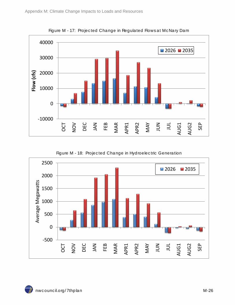
Appendix M: Climate Change Impacts to Loads and Resources
nwcouncil.org/7thplan M-26
Figure M - 17: Projected Change in Regulated Flows at McNary Dam
Figure M - 18: Projected Change in Hydroelectric Generation
-10000
0
10000
20000
30000
40000
OCT
NO
V
DEC
JAN
FEB
MAR
APR1
APR2
MAY
JUN
JUL
AUG
1
AUG
2
SEP
Flow
(cfs
)
2026 2035
-500
0
500
1000
1500
2000
2500
OCT
NO
V
DEC
JAN
FEB
MAR
APR1
APR2
MAY
JUN
JUL
AUG
1
AUG
2
SEP
Aver
age
Meg
awat
ts
2026 2035

Appendix M: Climate Change Impacts to Loads and Resources
nwcouncil.org/7thplan M-27
Table M - 3: Climate Induced Impacts to Energy Load/Resource Balance (aMW)
2026 2035
Winter Summer Winter Summer
Hydro Generation 700 -125 1,500 -140
Load -20 400 -40 750
Net (R-L) 720 -525 1,540 -890
Reservoir Storage Because of the climate-induced shift in unregulated flows and in demand for electricity, reservoirs will be used, to the extent possible, to realign the monthly pattern of hydroelectric generation to the changing monthly load shape. In fall and winter, for example, when demand should be lower, as much water as possible should be stored and held until summer when demand is expected to be higher. Due to operating constraints for non-power purposes (such as flood control and fish flow augmentation), however, it may not be possible to shift very much water from fall and winter to summer. On the positive side, because the snowpack is expected to be smaller, flood control elevations during spring months should be correspondingly higher, thus enabling more water to be stored and available for summer use.
Figure M - 19 shows the simulated change in aggregate average end-of-month storage content at Grand Coulee, Libby, Hungry Horse and Dworshak dams that would occur in 2026 and 2035 under a climate change scenario. Storage in this chart is measured in thousands of “second foot days” (KSFD). One KSFD is equivalent to roughly 2,000 acre-feet and 500 KSFD is equivalent to about one million acre-feet (MAF).
A breakdown of the results in that figure shows that, on average, the reservoir system stores water in December but that water is forced out in January. In March and April storage is down relative to a non-climate-change scenario. Again this may be due to constraints (minimum flow requirements) to keep salmon eggs submerged and to avoid stranding fry in the Columbia River during those months. The month of May shows an increase in storage, likely due to reduced flood control requirements. Finally, in the summer months through September, the additionally stored water (and more) is released for both power and fish requirements. These storage changes are not large relative to the aggregate storage capability of these four projects, which is about 7.8 million acre-feet. It appears that, on average, the storage at these four projects will be slightly lower going into the following year. This effect was not included in the analysis because the GENESYS runs were performed as refill studies. More detailed analysis will be done once the IPCC 5 AR5 data are downscaled and prepared for hydrologic studies.

Appendix M: Climate Change Impacts to Loads and Resources
nwcouncil.org/7thplan M-28
Figure M - 19: Climate Induced Change in Storage (Coulee, Libby, Horse and Dworshak)
Power Supply Adequacy In 2011, the Council adopted a resource adequacy standard that set the maximum likelihood of a future shortfall to be no more than 5 percent. This standard has been incorporated into the Regional Portfolio Model so that, in general, resource strategies developed by the model will produce power supplies that are adequate. Because climate change scenarios cannot, as yet, be included in Regional Portfolio Model analyses (see the section below), the purpose of this analysis is to assess whether a climate change scenario would alter any resource actions the region would take based on the power plan’s recommendations.
In order to assess whether resource actions would be affected during the action plan period (first six years), expected resources acquisitions from a Regional Portfolio Model scenario can be examined for adequacy for a normal case and for a climate change case. For this comparison, scenario 1B was used to extract the resource builds for a high-load path case for the years 2026 and 2035 (see Figure M - 15). Power supply adequacy was examined for both those years for both normal and climate change scenarios.
In both cases, the 2026 power supply was deemed adequate. However, that does not mean that climate change has no impacts. Figure M - 20a illustrates the 2026 expected monthly energy shortfalls for both the normal and climate change scenarios prior to the deployment of demand response resources. (After deployment, both scenarios show very little shortfall, which makes
-200
-100
0
100
200
300 O
CT
NO
V
DEC
JAN
FEB
MAR
APR1
APR2
MAY
JUN
JUL
AUG
1
AUG
2
SEP
Stor
age
(KSF
D)
2026 2035

Appendix M: Climate Change Impacts to Loads and Resources
nwcouncil.org/7thplan M-29
comparing the two scenarios difficult.) Figure M - 20b shows the 2035 expected monthly energy shortfalls.
As evident in Figure M - 20a, monthly shortfalls in winter decrease somewhat in the climate change scenario while monthly shortfalls in summer greatly increase. This supports the observation made above that the region is transitioning from a winter-only peaking region to one with both winter and summer peaks. Figure M - 20b illustrates the expected monthly energy shortfalls for 2035.
Figure M - 20a: 2026 Projected Change in Expected Loss of Load
Figure M - 20b: 2035 Projected Change in Expected Loss of Load
0
200
400
600
800
1000
1200
Oct
Nov
Dec
Jan
Feb
Mar
Ap1
Ap2
May
Jun Jul
Au1
Au2
Sep
Meg
awat
t-Ho
urs
Prior to Deployment of Demand Response
No CC CC
0
3000
6000
9000
12000
15000
18000
Oct
Nov
Dec
Jan
Feb
Mar
Ap1
Ap2
May
Jun Jul
Au1
Au2
Sep
Meg
awat
t-Ho
urs
No CC CC

Appendix M: Climate Change Impacts to Loads and Resources
nwcouncil.org/7thplan M-30
Climate Change Effects on the Seventh Plan For the 2035 high load case, the resulting loss-of-load probability under the climate change scenario grew to about 15 percent, which violates the maximum standard of 5 percent established by the Council. This means that for the 2035 high load case, additional resources would be needed to offset the temperature and flow impacts of climate change. However, the 2026 high load case indicated that no new resources were required under the climate change scenario to maintain adequacy. Therefore, the Council concluded that no new resource acquisitions would be needed until at least 2026 beyond those called for in the Seventh Power Plan’s resource strategy. This means that the climate change scenario analyzed for this appendix has no effect on this plan’s six year action plan.
For a medium load path case through 2035, in which only economic energy efficiency savings were acquired, no new resources for climate change were needed, thus setting a lower bound for climate-change required resource additions. Figure M - 21 illustrates the load conditions under which the region may need additional resources to offset the effects of climate change.
Figure M - 21: When Additional Resources may be needed to offset Climate Change
OTHER CLIMATE CHANGE IMPACTS Because river flows are likely to decrease in spring and summer, smolt (juvenile salmon) outmigration (journey to the ocean) and adult salmon returns will be affected. Lower river flows
20000
22000
24000
26000
28000
30000
2015 2020 2025 2030 2035
Load
(aM
W)
Annual Energy Load Forecast
New Resources For Climate Change Needed

Appendix M: Climate Change Impacts to Loads and Resources
nwcouncil.org/7thplan M-31
translate into lower river velocity and longer travel times to the ocean for migrating smolts. Lower river flows combined with higher air temperatures also means that water temperatures are likely to increase, another factor contributing to salmonoid fish stress and mortality. For example, based on this year’s experience, warm water appears to have been detrimental to larger sturgeon. However, other warm water species will likely fare better – possibly even thrive in warmer waters.
The projected shift in unregulated flows could:
Put greater flood control pressure on storage reservoirs and increase the risk of late fall or winter flooding;
Boost winter production of hydroelectric generation when Northwest demands are likely to drop due to higher average temperatures;
Reduce the size of the spring runoff and shift its peak to an earlier time;
Reduce late spring and summer river flows and potentially cause average water temperatures to rise, especially in the tributaries;
Jeopardize native fish survival, particularly salmon, steelhead and possibly sturgeon, by reducing the ability of the river system to meet minimum flow and water temperature requirements during the spring, summer and fall;
Reduce the ability of reservoirs to meet demands for irrigation water;
Reduce summer power generation at hydroelectric dams when Northwest demands and power market values will likely be higher; and
Affect summer and fall recreation activities.
Besides the impacts to river flows, hydroelectric generation and temperatures, climate change will affect the Northwest’s electricity interactions with other regions. Currently, both the Northwest and Southwest benefit from having different peak load periods. During the winter peak demand season in the Northwest, the Southwest generally has surplus capacity, which can be imported to help with winter reliability. In the summer months, the opposite is generally true and some of the Northwest’s hydroelectric capacity can be exported to help the Southwest meet its peak demand needs. This sharing of resources is cost effective for both regions.
Under a severe climate change scenario the Northwest could see increased summer demand with greatly decreased summer hydroelectric production. It is possible the Northwest could find itself having to plan for summer peak needs as well as for winter peaks. In that case, the Northwest would no longer be able to share its surplus capacity with the Southwest. This would obviously have economic impacts in the Southwest where additional generating resources may be needed to maintain summer service. This would likely raise the value of late summer energy in the West, thereby increasing the economic impact of climate change to the Northwest.

Appendix M: Climate Change Impacts to Loads and Resources
nwcouncil.org/7thplan M-32
All of the impacts described above are based on an analysis of a hydroelectric system operation using current drafting and filling constraints for both power and non-power purposes. It is unclear at this time how much flexibility the system has to modify certain constraints in order to better adapt hydroelectric generation with shifts in electricity load. For example, if reservoirs were allowed to be drafted deeper by summer’s end, the additional regulated flow and corresponding generation would benefit both migrating fish and electricity customers, and potentially late fall and early winter flood control. Unfortunately, making this change could affect other non-power users. However, it is prudent to review all constraints placed on the hydroelectric system operation in light of potential climate change impacts.
MODELING CLIMATE CHANGE IN THE REGIONAL PORTFOLIO MODEL Ideally, climate change uncertainty and its impacts to hydroelectric generation and loads would be included as one of the random variables in the Council’s Regional Portfolio Model. Unfortunately, this cannot be done at this time for several reasons. First, the data required to do so are not available. Second, even if the data were available, the Regional Portfolio Model is not equipped to accommodate it. Third, the relative likelihood of occurrence for each separate GCM climate change scenario is not known.
Figure M - 2 illustrates the mean forecasted temperature and precipitation changes in the Columbia River Basin for a number of climate change scenarios. Each point in this graph represents the result of a single GCM climate change scenario analysis. Three conclusions can be drawn from this figure; 1) each GCM result shows a net temperature increase, 2) nothing definitive can be said about the change in total annual volume of precipitation and 3) there is great uncertainty in both the temperature and precipitation forecasts.
The Regional Portfolio Model is a Monte Carlo computer program that assesses average power system cost and economic risk for many different resource plans. Each resource plan is, in essence, a potential supply curve of available new resources, including conservation, over the study horizon period. Each resource plan is examined over many different potential futures for the Northwest. Each future covers a 20-year period and draws from many random variables, including load, hydroelectric generation (flow conditions), electricity prices, fuel prices and carbon cost to assess costs. In order to incorporate climate change uncertainty into the model as a random variable, the relative likelihood of occurrence for each climate scenario shown in Figure M - 2 must be known. Then for each future examined, one particular climate change profile would be selected (i.e. one of the points in Figure M - 2) as one of the many random variables used for that particular future. This concept is illustrated graphically in Figure M - 22. In this figure, the mean forecasted temperature increase per year over a 20-year period is plotted for several different climate change scenarios (GCM1 through GCM4). In this example, a probability distribution is assigned to the set of scenarios, shown as the bell curve to the right of the graph. In this example, GCM2 and GCM3 are more likely to occur than GCM1 or GCM4 and thus they would be selected more often in the Monte Carlo

Appendix M: Climate Change Impacts to Loads and Resources
nwcouncil.org/7thplan M-33
simulation. Probability distributions for Northwest climate change scenarios, however, have not yet been developed.
Figure M - 22: Illustrative Probability Distribution for Climate Model Results
Unfortunately, this is only one problem that has to be overcome in order to incorporate climate change as a random variable into the Regional Portfolio Model. Once a climate scenario is chosen by the model, its long-term effects on load and on hydroelectric generation will have to be interpolated back into the 2015 to 2035 study horizon period. Methods for performing that interpolation have not been extensively explored, although an example of one method has already been discussed earlier in this appendix.
But in spite of these difficulties, progress is being made. The Bonneville Power Administration, the Corps of Engineers and the Bureau of Reclamation have initiated a regional process to collect, review and make available all climate change data related to river operations. This process is being developed under the auspices of the River Management Joint Operating Committee (RMJOC) and will ultimately result in a web-based database that will include climate change data needed to perform river operation analyses. Among other things, the additional data will include climate-change adjusted runoff forecasts and operating rule curves (as did the downscaled AR4 data). The Council supports this work and will actively participate in its development. Currently, the RMJOC is scheduled to complete its work to translate the AR5 results into useable data by the end of 2016 or by early 2017.

Appendix M: Climate Change Impacts to Loads and Resources
nwcouncil.org/7thplan M-34
CONCLUSIONS AND RECOMMENDATIONS Global circulation models all seem to agree that future temperatures will be higher but they differ on overall levels of precipitation. Some models suggest that the Northwest will be drier while others indicate more precipitation. But all the models predict less snow and more rain during winter months, resulting in a smaller spring snowpack. Winter electricity demands would decrease with warmer temperatures, easing the Northwest’s generating requirements. In the summer, increased demands driven by air conditioning and irrigation loads would rise and exacerbate the already tight market for electricity resources.
The development of the Seventh plan for the Northwest incorporates actions intended to address future uncertainties and their risks to electricity supply and to the economy. Such uncertainties include fluctuations in demand, fuel prices, changes in technology and increasing environmental constraints. Uncertainties related to climate change fall into two areas; 1) physical impacts that affect electricity demand and hydroelectric generation and 2) policies directed at reducing greenhouse gas emissions that affect resource operation and cost. The effect of policy decisions is described in more detail in Chapters 3 and 15. The physical effects of climate change have no effect on the resource acquisition or actions identified in this plan over the next six year period. However, the Council will continue to monitor and participate in regional efforts to better understand potential climate change and its effects on the power supply.

Seventh Northwest Conservation and Electric Power Plan
nwcouncil.org/7thplan N-1
APPENDIX N: DIRECT USE OF NATURAL GAS
Contents Economic Fuel Choices from Consumer’s Perspective...................................................................... 2
Background ................................................................................................................................... 2 Findings from the Sixth Plan Analysis ................................................................................................ 5 Analysis of Direct Use of Natural Gas For The Seventh Power Plan ................................................. 7
Findings from the 2014 analysis:.................................................................................................. 10 Conclusions and Recommendations ............................................................................................ 12
Revised Council Policy Statement Regarding Direct Use of Natural Gas ................................. 13
List of Figures and Tables Figure N - 1: Primary Space Heating Fuel in Single Family Homes ................................................... 3 Figure N - 2: RBSA 2012 Single Family Distribution on Water Heater Fuel ....................................... 3 Table N - 1: Results from Sixth Plan’s Analysis of Direct Use of Natural Gas .................................... 6 Figure N - 3: Illustrative Example of Marginal Market Share SF- Washington Less Than or Equal To 55 Gallon Water Heating ................................................................................................................... 8 Figure N - 4: Illustrative Example of Marginal Market Share SF- Oregon Less Than or Equal To 55 Gallon Water Heating ........................................................................................................................ 9 Figure N - 5: Reduction in Electricity Usage by 2035 (aMW) ............................................................. 9 Figure N - 6: Change in Natural Gas Usage by 2035(TBTU) ........................................................... 10 Figure N - 7: Forecasted average market share for water heaters greater than 55 gallons in capacity (BAU) .............................................................................................................................................. 11 Figure N - 8: Forecasted average market share for water heaters 55 gallons or less in capacity .... 11

Appendix N: Direct Use of Natural Gas
nwcouncil.org/7thplan N-2
ECONOMIC FUEL CHOICES FROM CONSUMER’S PERSPECTIVE
Background The issue of whether it is better to use natural gas directly in hot water heaters and furnaces than to generate electricity by burning natural gas and then use electricity to heat water and homes has been raised during the development of each of the Council’s plans, starting with its first. Over the years the Council has conducted multiple studies to address this issue. The issue has been described by different names including fuel choice, fuel switching, direct use of gas, and total energy efficiency.
The region’s natural gas companies sued the Council after the first power plan; one of the few law suits the Council has had. The concern was that the Plan recommended that Bonneville acquire energy efficiency (through its customer utilities) by providing financial incentives to encourage consumers to install measures that improved electricity efficiency. The gas companies argued that these incentives would disadvantage natural gas companies and encourage more use of electricity. Over time the concerns have morphed into arguments that direct use of natural gas is more thermodynamically efficient (i.e. uses less total energy to produce the same end use service) and hence more benign for the environment.
In 1994, the Council analyzed the economic efficiency of converting existing residential electric space and water heating systems to gas systems.1 The results of that study found potential savings of over 730 average megawatts of cost-effective fuel-switching opportunities within the region. However, the Council has not included programs in its power plans to encourage the direct use of natural gas, or the promotion of the conversion of electric space and water heat to natural gas. The basis for this policy recommendation is that all of the Council’s prior analyses have indicated that fuel choice markets are working well. Since the large electricity price increases around 1980, the electric space heating share has stopped growing in the region while the natural gas space heat share in existing homes increased from 26 to 37 percent. A survey of new residential buildings conducted in 2004 for the Northwest Energy Efficiency Alliance (NEEA) found that nearly all new single-family homes constructed where natural gas was available had gas-fired forced air heating systems.2 The survey also found an increased penetration of natural gas heating in the traditionally electric heat dominated multi-family market, especially in larger units and in Washington.3 Fuel
1 Northwest Power Planning Council. “Direct Use of Natural Gas: Analysis and Policy Options”. Issue Paper 94-41. Portland, OR. August 11, 1994. 2 Northwest Energy Efficiency Alliance, Single-Family Residential New Construction Characteristics and Practices Study. Portland, OR March 27, 2007. Prepared by RLW Analytics.
3 Northwest Energy Efficiency Alliance, MultiFamily Residential New Construction Characteristics and Practices Study. Portland, OR June 14, 2007. Prepared by RLW Analytics.

Appendix N: Direct Use of Natural Gas
nwcouncil.org/7thplan N-3
conversion of existing houses to natural gas has been an active market as well, often promoted by dual-fuel utilities.
The most recent study available, the 2012 Residential Building Stock Assessment (RBSA) also conducted by NEEA, indicates that the trend of decreasing market share of electricity and increasing market share of natural gas is continuing. As Figures N - 1 shows, between 1992 and 2012 regional surveys the market share of both electric space and water heating in single family homes has declined while the market share of natural gas used for these same end uses has increased. Single family electric space heating dropped from about 60 percent in 1992 to about 33 percent by 2012 and electric water heating’s market share declined from 76 percent to about 55 percent during the same period.
Figure N - 1: Primary Space Heating Fuel in Single Family Homes
Figure N - 2: RBSA 2012 Single Family Distribution on Water Heater Fuel
The Council’s analytical findings and policy on the issue of direct use of natural gas/fuel switching have been very consistent. All of the Council’s prior analysis found that while direct use of natural
0% 10% 20% 30% 40% 50% 60% 70%
Electric
Gas
Oil
Wood/Pellets
Propane
RBSA 2012 PNRES 1992
52% 38%
55% 59% 55%
45% 59%
43% 40% 43%
3% 2% 2% 1% 2%
ID MT OR WA Region
RBSA 2012 Single Family Distribution on Water heater Fuel
Electricity Gas Propane
Market share of electricity as the primary space heating fuel has declined over the past two decades.
Market share of electricity as the water heating fuel varies across the states

Appendix N: Direct Use of Natural Gas
nwcouncil.org/7thplan N-4
gas is often more thermodynamically efficient than using electricity generated from natural gas, its economic efficiency (i.e., whether direct use of natural gas is lower cost) depends on the specific situation with respect to the relative price of natural gas and electricity, space and/or water heating energy use, the cost and efficiency of space and water heating systems, and access to natural gas service.
The Council’s policy, adopted in its first plan, is that fuel switching is not conservation under the Northwest Power Act, which defines conservation as “any reduction in electric power consumption as a result of increases in the efficiency of energy use, production, or distribution.”4 Further, the Council has determined, on the basis of its prior analysis, that fuel choice markets are reasonably competitive and that those markets should be allowed to work without interference. Thus, the current Council policy, which has been reaffirmed in each of past three plans, is:
In light of changing technologies and energy prices and growing climate concerns, the Council was again asked to look at the direct use of natural gas issue in the Sixth Power Plan. The analysis was called for in the Action Plan (ANLYS-16) for the Sixth Power Plan. The Council conducted extensive analysis of the consumer options from two specific approaches. The first was to determine which residential space and water heating systems have the lowest total resource cost (TRC) while presenting an acceptable level of risk to the region. The second objective was to determine whether the retail market conditions will lead consumers to generally choose those same space conditioning and water heating systems. If the systems selected based on the regional economic and risk perspective are similar to those selected based on consumer economics, then it would suggest that no policy intervention is needed.
4 [Northwest Power Act, §3(3), 94 Stat. 2698.]
Council Policy Statement Regarding Direct Use of Natural Gas
The Council recognizes that there are applications in which it is more energy efficient to use natural gas directly than to generate electricity from natural gas and then use the electricity in the end-use application. The Council also recognizes that in many cases the direct use of natural gas can be more economically efficient. These potentially cost-effective reductions in electricity use, while not defined as conservation in the sense the Council uses the term, are nevertheless alternatives to be considered in planning for future electricity requirements.
The changing nature of energy markets, the substantial benefits that can accrue from healthy competition among natural gas, electricity and other fuels, and the desire to preserve individual energy source choices all support the Council taking a market-oriented approach to encouraging efficient fuel decisions in the region.

Appendix N: Direct Use of Natural Gas
nwcouncil.org/7thplan N-5
FINDINGS FROM THE SIXTH PLAN ANALYSIS The analysis conducted pursuant to the Sixth Plan Action Item found that nearly three quarters (73 percent) of the market segments studied did not find it economically advantageous to switch their space conditioning and/or water heating fuel source, as shown in Table N - 1. However, approximately one half of these market segments, all of which use electricity for space conditioning and/or water heating found that it was economical to upgrade the efficiency of their equipment. The 223 average megawatts of savings from these efficiency improvements were already captured in the Council’s conservation supply curves and included in the Sixth Power Plan.
Table N - 1 also shows that for 22 percent of the market segments considered in the analysis the Council found that conversion from electric space heating and/or water heating to gas space and/or water heating was the most economical choice. If all of these households converted to natural gas regional electrical loads would be reduced by roughly 360 average megawatts and regional natural gas consumption would increase by just over 15 trillion BTU by the end of the 20-year period (2029). In aggregate across all market segments and excluding savings from efficiency improvements, a regional resource portfolio that reflects the economical selection of space conditioning and water heating systems would reduce regional electric loads by just under 340 average megawatts and increase regional natural gas consumption by slightly more than 13 trillion BTU.

Appendix N: Direct Use of Natural Gas
nwcouncil.org/7thplan N-6
Table N - 1: Results from Sixth Plan’s Analysis of Direct Use of Natural Gas
Segments
Represented
No.
House-
holds/yr
20-year
Total
House-
holds
Share of
Total
Existing
Use
(aMW/yr)
Existing Use
(MMBTU/yr)
Annual
Change in
Use
(aMW/yr)
Change in
Use
(aMW by
20th yr)
Replace w/Same Fuel & Same Equipment 20
48,412
968,235 37.3% 4.92 2,500,094 - -
w/Higher Efficiency Space Heating Equipment Only 14
1,807
36,145 1.4% 1.96 - (1)
(10)
w/Higher Efficiency Water Heating Equipment Only 10
33,439
668,785 25.8% 21.51 - (6)
(118)
w/Higher Efficiency Space & Water Heating Equipment 14
11,142
222,835 8.6% 15.26 - (5)
(95)
Sub-Total 58 94,800
1,895,999 73.1% 43.65 2,500,094
(11)
(223)
Convers. fr Electricity to Gas
Space Heating only 11 1,520
30,400 1.2% 1.57 -
(1.55)
(31)
Water Heating only 6 21,197
423,940 16.3% 8.05 -
(8.05) (161)
Space & Water Heating 6 5,745
114,900 4.4% 8.49 -
(8.29)
(166)
Sub-Total 23 28,462
569,240 21.9% 18.11 -
(18)
(358)
Conversions from Gas to Electricity
Space Heating only 0 - - 0.0% - - - -
Water Heating only 6 6,262
125,240 4.8% 0.10 98,713
1.21 24
Space & Water Heating 0 - - 0.0% - - - -
Sub-Total 6 6,262
125,240 4.8% 0.10 98,713
1
24
Conversions from Electric Space Heating and Gas Water Heating to Gas Space Heating and Electric Water Heating
8 168
3,360 0.1%
0.16 2,648 (0.13)
(3)
Totals 95 129,692 2,593,839 100% 58 2,601,455 (27.97) (559)
Changes Net of Efficiency 37 34,892 697,840 27% 18 101,361 (16.81)
(336)

Appendix N: Direct Use of Natural Gas
nwcouncil.org/7thplan N-7
Using the findings from the extensive analysis done following the adoption of the Sixth Power Plan, the assessment for the Seventh Power Plan focused on those market and end use segments that promised the best economic options for conversion from electricity to natural gas. The market segments with the largest potential and most favorable economics were existing single family homes with electric water heating and natural gas space heating.
ANALYSIS OF DIRECT USE OF NATURAL GAS FOR THE SEVENTH POWER PLAN The Seventh Power Plan analysis focused at the potential shift from electricity to natural gas in the single family water heating market. The analysis considers two water heater tank sizes. This was done to reflect the fact that beginning in 2015, the federal appliance standards establish different minimum efficiency levels by water heater size category, one for larger than 55 gallon capacity water heaters and another for water heaters with 55 gallon or lower capacity.
As noted previously, pursuant the Action Item ANLYS-16 in the Sixth Plan, the Council conducted a study of the direct use of natural gas as part of a continued effort to identify whether there is a need for programs encouraging consumers to switch from electric space heat and water heat to natural gas space heat and water heat. The Council’s 2012 study’s findings were reported in Council document 2012-01, “Direct Use of Natural Gas: Economic Fuel Choices from the Regional Power System and Consumer’s Perspective”. https://www.nwcouncil.org/reports/2012-01/.
This study analyzed 94 residential market segments and compared the consumer least-cost retrofit options to the water heating options that would be chosen given a total resource cost test. Overall, the study found that there was general alignment between the water heating systems that are least cost to the consumer and least total cost to the region. This alignment indicated that price signals exist which encourage a shift to the direct use of natural gas. Whereas price signals have been shown to be in place which encourage shifting to the direct use of natural gas, market studies on how consumers make choices have shown repeatedly that consumers do not choose based on price alone. Rather, these studies suggest that consumers are “rationally inattentive” to prices alone.5 Given this knowledge about consumers, the question becomes, even when price signals indicate a lowest-cost option, what will consumers actually choose?
To investigate the question of what consumers are likely to choose, in July 2014 the Council commissioned Systematic Solutions, Inc. (SSI) to perform a small-scale study on a targeted subset of eight segments from the original 94 residential market segments. This purpose of this study was to apply a consumer choice model to consumers’ expected water heating choices to estimate the share of consumers who would actually select the least-cost water heating system. The Council commissioned SSI to develop both a “spreadsheet model” version of consumer choice analysis and
5 Matejla, F. and Alisdair McKay, Rational Inattention to Discrete Choice: A New Foundation for the Multinomial Logit Model”, May 2014.

Appendix N: Direct Use of Natural Gas
nwcouncil.org/7thplan N-8
to conduct an analysis using the same assumptions in ENERGY 2020, the Council’s long-term load forecast model.
Using Consumer Choice approach, two alternative scenarios were explored.
1. Business-As-Usual – This case assumes the market share for each choice of water heating technologies depends on the relative perceived cost of that technology compared to all other choices. The results provide a baseline of expected future behavior.
2. Least Cost – This case assumes that lowest life cycle cost technology takes 100 percent of the market. This case is identical to that assumed in the Council’s 2012 analysis. It represents the maximum economic potential from switching fuels from the consumer, rather than regional perspective.
Figures N - 3 and N - 4 below illustrate the results of this analysis using the average electricity and natural gas prices (i.e., retail cost) for Washington and Oregon states. Note that analysis starts with 100 percent electric water heater saturation in both states since the “base condition” only includes homes with electric water heating. However due to differences in electricity prices and natural gas availability the marginal market shares are different between the two states.
Figure N - 3: Illustrative Example of Marginal Market Share SF- Washington Less Than or Equal To 55 Gallon Water Heating
Existing 2014 BAU Case 2035 Least Cost Case 2035
0%
10%
20%
30%
40%
50%
60%
70%
80%
90%
100%
Condensing Gas
Instant Gas
Gas Tank
HeatPumpWH
Electric Resistance
Figure N-3 shows that in Washington single family households with electric resistance water heating in 2014, 100% would convert to heat pump water heaters by 2035 if they selected the Least Cost option.
Under the BAU scenario these same households’ replacement water heaters would be divided between the five technology choices.

Appendix N: Direct Use of Natural Gas
nwcouncil.org/7thplan N-9
Figure N - 4: Illustrative Example of Marginal Market Share SF- Oregon Less Than or Equal To 55 Gallon Water Heating
Figure N - 5 shows the reduction in electricity usage (in average megawatts) when comparing regional electricity consumption for water heating in 2035 under the Least Cost scenario compared to the consumption under the Business as Usual case.
Figure N - 5: Reduction in Electricity Usage by 2035 (aMW)
Figure N - 6 shows change in regional natural gas consumption by 2035 for the consumers (i.e., direct use) and for the electricity generators (Northwest Utility) and the net total consumption.
0%
10%
20%
30%
40%
50%
60%
70%
80%
90%
100%
Existing 2014 BAU Case 2035 Least Cost Case 2035
Condensing Gas Instant Gas
Gas Tank
HPWH
Electric Resistance
114
20 17 24
54
-
20
40
60
80
100
120
Northwest
Idaho
Montana
Oregon
Figure N-4 shows that in Oregon single family households with electric resistance water heating in 2014, 100% would convert to an natural gas water heater by 2035 if they selected the Least Cost option.
Under the BAU scenario these same households’ replacement water heaters would be divided between the five technology choices.

Appendix N: Direct Use of Natural Gas
nwcouncil.org/7thplan N-10
Figure N - 6: Change in Natural Gas Usage by 2035(TBTU)
Findings from the 2014 analysis: Analysis shows:
If consumers choose water heating fuel source based on least cost there would be reduction in regional electricity consumption, about 1000 gigawatt-hours (GWh) per year or 114 average megawatts (aMW) by 2035
When lower demand from electric power generation is taken into account, regional natural gas consumption could also decline about 2.7 trillion British thermal units (Tbtu).
Using the consumer choice modeling approach in the Council’s long-term model, the forecast of water heating market share for the draft Seventh Plan analysis shows continued trend in the switch from electricity as the fuel for water heating to natural gas. The speed of conversion reflected in the market share trends vary depending on the size of water heaters and consumer’s needs. Figures N – 7 and N – 8 show the trend in electric and gas water heating market share for tanks with greater than 55 gallon capacity (N – 7) or less and those with 55 gallon or less capacity (N – 8). As can be seen from these figures, gas water heating’s market share significantly increases in the larger tank category, while market shares for gas decline slowly in the smaller capacity tank category. This reflects the fact that gas and electric water heating technologies in the smaller capacity tank category are not significantly different in cost throughout the planning period.
-8.0
-6.0
-4.0
-2.0
0.0
2.0
4.0
6.0
2015 2020 2025 2030 2035
Consumer
NW Utility
NW Utility and Consumer
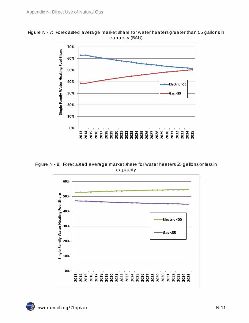
Appendix N: Direct Use of Natural Gas
nwcouncil.org/7thplan N-11
Figure N - 7: Forecasted average market share for water heaters greater than 55 gallons in capacity (BAU)
Figure N - 8: Forecasted average market share for water heaters 55 gallons or less in capacity
0%
10%
20%
30%
40%
50%
60%
70%
2013
20
14
2015
20
16
2017
20
18
2019
20
20
2021
20
22
2023
20
24
2025
20
26
2027
20
28
2029
20
30
2031
20
32
2033
20
34
2035
Sing
le F
amily
Wat
er H
eatin
g Fu
el S
hare
Electric >55
Gas >55
0%
10%
20%
30%
40%
50%
60%
2013
20
14
2015
20
16
2017
20
18
2019
20
20
2021
20
22
2023
20
24
2025
20
26
2027
20
28
2029
20
30
2031
20
32
2033
20
34
2035
Sing
le F
amily
Wat
er H
eatin
g Fu
el S
hare
Electric <55
Gas <55

Appendix N: Direct Use of Natural Gas
nwcouncil.org/7thplan N-12
The findings from the 2014 Direct Use of Natural Gas study were reviewed by the Council and then released for public comment. Feedback from regional entities on the analysis specifically ask for comments on these three questions:
1) “Are there data that show the trends Council is observing are not correct?” 2) “If one were to decide to intervene in water heating fuel choice market, are their practical
program designs to identify consumers who could convert to gas water heating when the option is available?”
3) “Are there future market conditions (fuel prices, technology changes, non-price factors) such that the competition between natural gas and electricity warrant Council intervention in the market?
The Council received written comment from: two private citizens, Energy Trust of Oregon, City of Ellensburg Municipal Utility (electric and natural gas service area), NW Gas Association, Cascade Natural Gas, Northwest Natural, Puget Sound Energy, and Portland General Electric. In addition the Council received three academic papers on the topic from Portland State University graduate students studying Demand Response.
A summary of the feedback received and the details of each respondent’s comments are available from the council website. http://www.nwcouncil.org/energy/powerplan/7/DUG7thPlan
Conclusions and Recommendations In preparation for the draft Seventh Power Plan, the Council reviewed its prior findings on the economics of direct use of natural gas to displace residential space and/or water heating. An updated analysis was performed that focused on the eight market segments identified in the Council’s 2012 assessment as providing both consumers and the region with economic benefits through conversion from electricity to natural gas. The updated analysis estimated the share of single family homes with electric water heating and natural gas space heating that would find economic benefits by conversion to natural gas water heating when their existing electric water heater required replacement. Two estimates were made. The first, which is comparable to the 2012 analysis, assumed that in all cases the most economical (i.e. lowest life cycle cost) water heating fuel type would be selected. The second case assumed that consumers would not always select the lowest cost option due to other “non-economic” barriers to conversion. This case found that fewer, but still a significant share of households, would alter their existing water heating fuel. Moreover, based on historical fuel selection trends, the study suggests that natural gas will continue to gain space and water heating market share while electricity’s share of these end uses will continue to decrease.
Given the above findings and the public comments received, the Council decided to retain its current policy with a minor modification: the word “preserve” in the original statement was replaced with the work “promote”.

Appendix N: Direct Use of Natural Gas
nwcouncil.org/7thplan N-13
Revised Council Policy Statement Regarding Direct Use of Natural Gas
The Council recognizes that there are applications in which it is more energy efficient to use natural gas directly than to generate electricity from natural gas and then use the electricity in the end-use application. The Council also recognizes that in many cases the direct use of natural gas can be more economically efficient. These potentially cost-effective reductions in electricity use, while not defined as conservation in the sense the Council uses the term, are nevertheless alternatives to be considered in planning for future electricity requirements.
The changing nature of energy markets, the substantial benefits that can accrue from healthy competition among natural gas, electricity and other fuels, and the desire to promote informed individual energy source choices all support the Council taking a market-oriented approach to encouraging efficient fuel decisions in the region.

Seventh Northwest Conservation and Electric Power Plan
nwcouncil.org/7thplan 15-1
APPENDIX O: INITIAL SCENARIO ANALYSIS Contents
Introduction ....................................................................................................................................... 4 Scenario Analysis .............................................................................................................................. 4
Scenarios Requiring Updates to Input Assumptions....................................................................... 5 Testing Resource Strategies ............................................................................................................. 5
Resource Strategy Definition ......................................................................................................... 5 The Regional Portfolio Model ......................................................................................................... 5 Uncertainty in System Costs .......................................................................................................... 6 Resource Strategy Adequacy ........................................................................................................ 8
Developing Scenarios ....................................................................................................................... 9 Scenarios without Carbon Costs .................................................................................................... 9
Existing Policy ............................................................................................................................ 9 Maximum Carbon Reduction - Existing Technology ................................................................... 9 Maximum Carbon Reduction - Emerging Technology ................................................................ 9 Regional 35 Percent RPS ........................................................................................................ 10 No Demand Response - No Carbon Cost................................................................................. 11 Low Fuel and Market Prices - No Carbon Cost ........................................................................ 11 No Coal Retirement .................................................................................................................. 13 Lower Conservation - No Carbon Cost ..................................................................................... 13
Scenarios with Carbon Costs ....................................................................................................... 13 Social Cost of Carbon - Mid-Range and High-Range ............................................................... 13 Carbon Cost Risk ..................................................................................................................... 14 Resource Uncertainty – Planned and Unplanned Loss of a Major Resource ............................ 15 Faster and Slower Conservation Deployment .......................................................................... 15 No Demand Response – Carbon Cost ..................................................................................... 15 Low Fuel and Market Prices – Carbon Cost ............................................................................. 15 Increased Reliance on External Markets .................................................................................. 15
Examining Results ........................................................................................................................... 16 Energy Efficiency Resources ....................................................................................................... 17 Demand Response ...................................................................................................................... 22 Renewable Generation ................................................................................................................ 24 Natural Gas-Fired Generation ...................................................................................................... 27 Carbon Emissions ........................................................................................................................ 31
Maximum Carbon Reduction – Emerging Technology .............................................................. 37 Federal Carbon Dioxide Emission Regulations ........................................................................ 43
Resource Strategy Cost and Revenue Impacts ............................................................................ 47

Appendix O: Initial Scenario Analysis
nwcouncil.org/7thplan O-2
List of Figures and Tables
Figure O - 1: How to Interpret Probability Distribution Graphs ........................................................... 7 Figure O - 2: Distribution of System Costs Example .......................................................................... 7 Table O - 1: RPS Requirement Scenario Assumptions .................................................................... 10 Table O - 2: Percent of Obligated Load Assumptions ...................................................................... 11 Figure O - 3: Range of Natural Gas Prices ...................................................................................... 12 Figure O - 4: Range of Electricity Prices .......................................................................................... 13 Table O - 3: Social Cost of Carbon Assumptions (2012$/Metric Ton of CO2) .................................. 14 Figure O - 5: Average Resource Development in Least Cost Resource Strategy by 2035 in Alternative Scenarios ...................................................................................................................... 17 Figure O - 6: Average Net Regional Load After Accounting for Cost-Effective Conservation Resource Development ................................................................................................................... 18 Figure O - 7: Amount of Cost-Effective Conservation Resources Developed Under Different Scenarios ........................................................................................................................................ 20 Figure O - 8: Efficiency Potential by Sector and Levelized Cost by 2035 ......................................... 21 Figure O - 9: Monthly Shape of 2035 Efficiency Savings ................................................................. 22 Figure O - 10: Demand Response Resource Supply Curve ............................................................. 23 Figure O - 11: Demand Response Resource Development by 2021 Under Alternative Scenarios ... 24 Figure O - 12: Average Renewable Resource Development by Scenarios by 2021, 2026 and 2035 26 Figure O - 13: Probability of New Natural Gas-Fired Resource Development by 2021 .................... 28 Figure O - 14: Probability of New Natural Gas-Fired Resource Development by 2026 .................... 29 Figure O - 15: Average New Natural Gas-Fired Resource Development ......................................... 30 Figure O - 16: Average Annual Dispatch of Existing Natural Gas-Fired Resources ......................... 31 Figure O - 17: Carbon Regulatory Cost or Price and Societal Cost of Carbon Tested in Scenario Analysis ........................................................................................................................................... 32 Figure O - 18: Average System Costs and PNW Power System Carbon Emissions by Scenario in 2035 ................................................................................................................................................ 33 Figure O - 19: Average Annual Carbon Emissions by Carbon Reduction Policy Scenario ............... 34 Figure O - 20: Cumulative 2016 to 2035 Carbon Emissions Reductions for Carbon Policy Scenarios ........................................................................................................................................................ 35 Table O - 4: Average Cumulative Emissions Reductions and Present Value Cost of Alternative Carbon Emissions Reduction Policies Compared to Existing Policy Scenario ................................. 36 Table O - 5: Energy Efficiency Emerging Technologies Modeled in the RPM in the Maximum Carbon Reduction – Emerging Technology Scenario ................................................................................... 39 Table O - 6: Non-Carbon Dioxide Emitting Generating Emerging Technologies Modeled in the RPM in the Maximum Carbon Reduction – Emerging Technology Scenario ............................................ 39 Figure O - 21: Distribution of Annual Carbon Dioxide Emissions Under Maximum Carbon Reduction Scenarios With and Without Emerging Technology ......................................................................... 40 Figure O - 22: Difference in Annual Resource Dispatch Between Maximum Carbon Reduction – Existing Technology Scenario and Maximum Carbon Reduction – Emerging Technology Scenario 41 Table O - 7: Enhance Geothermal and Small Modular Reactor Emerging Technologies’ Potential Availability and Cost ........................................................................................................................ 43 Table O - 8: Utility Scale Solar PV with Battery Storage Emerging Technologies’ Potential Availability and Cost .......................................................................................................................................... 43 Table O - 9: Pacific Northwest States’ Clean Power Plan Final Rule CO2 Emissions Limits ............ 44

Appendix O: Initial Scenario Analysis
nwcouncil.org/7thplan O-3
Table O - 10: Nameplate Capacity of Thermal Generation Covered by EPA Carbon Emissions Regulations Located Within Northwest States ................................................................................. 45 Figure O - 23: Average Annual Carbon Dioxide Emissions for Least Cost Resource Strategies by Scenario for Generation Covered by the Clean Power Plan and Located Within Northwest States . 47 Figure O - 24: Average Net Present Value System Cost for the Least Cost Resource Strategy by Scenario With and Without Carbon Tax Revenues .......................................................................... 48 Table O - 11: Average Net Present Value System Cost with Carbon Cost and Incremental Cost Compared to Existing Policy, No Carbon Risk Scenario .................................................................. 49 Figure O - 25: Annual Forward-Going Power System Costs, Including Carbon Costs .................... 50 Figure O - 26: Annual Forward-Going Power System Costs, Excluding Carbon Tax Revenues ..... 51 Figure O - 27: Index of Historical and Forecast Utility Revenue Requirements ............................... 52 Figure O - 28: Electricity Average Revenue Requirement per MWh Excluding Carbon Tax Revenues ........................................................................................................................................ 53
Appendix O: Initial Scenario Analysis
nwcouncil.org/7thplan O-4
INTRODUCTION Not all of the scenarios and sensitivity studies analyzed during the development of the draft Seventh Power Plan were updated or revised for the final Seventh Power Plan. However, the results of the draft plan’s scenario analysis did inform the resource strategy and actions included in the final Seventh Power Plan. This appendix describes all of the scenarios and sensitivity studies analyzed for the draft plan. It also discusses their principal findings and implications for the major elements of the Seventh Power Plan’s resource strategy. All of the findings in this appendix appeared in either Chapter 3 or Chapter 15 of the draft Seventh Power Plan. These chapters have been edited to reduce the overlap between those chapters while retaining major findings.
SCENARIO ANALYSIS The Seventh Power Plan’s resource strategy is based on analysis of over 20 scenarios and sensitivity studies. Scenarios combined elements of the future that the region controls, such as the type, amount and timing of resource development, with factors the region does not control, such as natural gas and wholesale market electricity prices. Sensitivity studies alter one parameter in a scenario to test the how the least-cost resource strategy is affected by that input assumption. For example, several scenarios were run with and without future carbon cost to assess the impact of that input assumption on the various components of the least cost resource strategy.
All of the scenarios evaluated for the plan include the same range of uncertainty regarding future fuel prices, hydropower conditions, electricity market prices, capital costs, and load growth. However, several scenarios were specifically designed to provide insights into the cost and impacts of alternative carbon dioxide emissions reduction policies. These included either the federal government’s estimates of the societal damage cost of carbon dioxide emissions or the economic risk associated with future carbon dioxide regulation or pricing or “non-pricing” policies. Each of these scenarios assumed differing levels of carbon dioxide damage or regulatory cost. Also, as noted above, several sensitivity studies were conducted to assess the impact of such factors as the near term pace of conservation development, lower natural gas and wholesale electricity prices, greater reliance on external markets, or the loss of major resources.
Each scenario and sensitivity analysis tested thousands of potential resource strategies against 800 alternative future conditions to identify the least cost and lowest economic risk resource portfolios. Since the discussion of the elements of the resource strategy draws on those scenarios and sensitivity studies, an introduction to the scenarios and studies and their findings is needed. Each scenario or sensitivity study was designed to explore specific components of resource strategies (e.g. strategies with and without demand response). Therefore, the following discussion of findings compares different combinations of scenarios and sensitivity studies. That is, not all scenarios or sensitivity studies “stress test” the same element of a resource strategy, so not all provide useful insight regarding that element.

Appendix O: Initial Scenario Analysis
nwcouncil.org/7thplan O-5
Scenarios Requiring Updates to Input Assumptions To fully consider and respond to the comments received, the Council chose to update seven of the twenty-one scenario analyses and sensitivity studies it conducted for the draft plan with revised input assumptions based on public comment. The updated results of these seven scenarios and of the three additional scenarios suggested by public comment appear in Chapters 3 and 15. The scenarios results discussed in this appendix are those presented in the draft Seventh Power Plan.
TESTING RESOURCE STRATEGIES Resource Strategy Definition A resource strategy is a plan on how to acquire resources. It includes two decision points for a utility. When a utility planner needs to start planning for a resource and when a utility needs to start the construction of a resource. Because of uncertainty about the future, it makes sense to have circumstances where a utility would plan for a resource but choose not to construct it. Thus, each of these decisions must be treated distinctly.
A scenario is a different set of assumptions about future conditions. Scenarios can examine things such as the effect of enacting new legislation on the region’s power system or the effect of market regime changes on the power system. Generally, resource strategies reflect decisions that can be made by utilities, whereas scenarios reflect circumstances beyond the control of a utility. A resource strategy is considered robust if it exhibits both low cost and low risk across many different scenarios.
The Regional Portfolio Model The Regional Portfolio Model (RPM) is used to estimate the system costs of a resource strategy under a given scenario. The RPM is described exhaustively in Appendix L. The RPM tests a wide range of resource strategies including the amount of conservation developed, the amount of demand response optioned and the amount of thermal and renewable resources optioned across 800 potential futures. For each of the 800 potential futures examined, the RPM estimates capital costs for constructing new resources and operating costs of new and existing resources, as described in the previous section of this chapter. Each future then results in an estimate of the system costs.
One of the characteristics of a least-cost resource strategy in the RPM is that options for new generation and DR that are not built in at least one of the 800 futures are removed. That is, it is assumed that these options were not established until there was at least some probability that they would be exercised. Therefore, least cost resource strategies identified in the RPM recommend that options be taken at specific times in the future. In all scenarios examined and for all resources considered, having open options at every opportunity (i.e. continuous optioning) is more expensive. Maintaining these options strictly for crucial times should be a less costly approach for regional utilities to meet the needs of their system.
Resource strategies that minimize both cost and risk are considered optimal for a scenario. The RPM minimizes system cost by seeking resource strategies that reduce the average of the 800 future system cost estimates. The model minimizes system risk by seeking resource strategies that
Appendix O: Initial Scenario Analysis
nwcouncil.org/7thplan O-6
minimize the average of the 80 most expensive future system cost estimates. In this case “optimal” is limited to a comparison of the range of strategies tested by the RPM. Because of the complexity of the system cost calculation in the RPM, it is impossible to guarantee an optimal result without calculating every possible resource strategy. Modern computers are not yet powerful enough to complete this level of calculation in a reasonable amount of time. Instead some enhanced methods of searching through the resource strategies were used. Further discussion of this is found in Appendix L.
Uncertainty in System Costs As described in the previous section, each resource strategy results in a distribution of system costs. These distributions highlight the fact that future system costs are unknown. Figure O - 1 illustrates the cost distributions for two different strategies and Figure O - 2 gives an example of the system cost distribution for several different scenarios, which will be detailed later in this chapter.
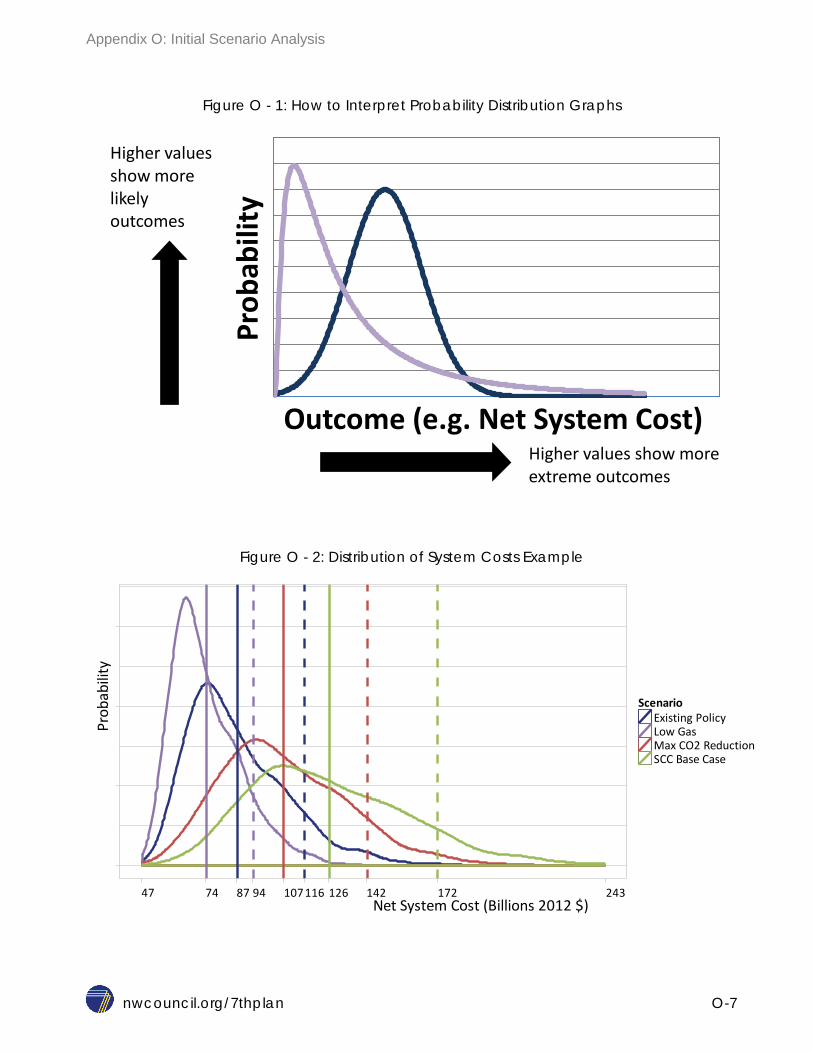
Appendix O: Initial Scenario Analysis
nwcouncil.org/7thplan O-7
Figure O - 1: How to Interpret Probability Distribution Graphs
Figure O - 2: Distribution of System Costs Example
Prob
abili
ty
Outcome (e.g. Net System Cost) Higher values show more extreme outcomes
Higher values show more likely outcomes
47 74 87 94 107116 126 142 172 243Net System Cost (Billions 2012 $)
Prob
abili
ty
ScenarioExisting PolicyLow GasMax CO2 ReductionSCC Base Case

Appendix O: Initial Scenario Analysis
nwcouncil.org/7thplan O-8
When testing resource strategies, the uncertainty represented by the cost distribution associated with a scenario helps describe the impact of a scenario. How the impact is interpreted depends on the scenario. For example, in a scenario where low gas prices are assumed to persist throughout the study the power system costs are much lower than a scenario that assumes broader range of future gas prices. However, while the lower cost in this scenario would likely be a boon for the consumers of electricity, the least cost resource strategy for this scenario might be highly dependent upon future conditions that are outside of the control of the Northwest. In contrast, under a scenario which assumes retirements of generating resources, regional decision-makers can implement a least cost resource strategy that might include more conservation, options for demand response and construction of new thermal generators. Therefore, when there is uncertainty in future system cost it is important to understand the sources of that uncertainty and specifically whether options to mitigate that cost risk are within the control of the region. The resource strategy described in Chapter 3 was developed by considering these criteria.
Resource Strategy Adequacy A detailed description of how the Council’s resource adequacy standard is implemented in the Regional Portfolio Model is provided in Chapter 11. The RPM tests a resource strategy for adequacy by testing whether its resources meet a minimum build requirement for both energy and capacity adequacy standards. In the event that the strategy does not have sufficient resource to meet adequacy standards, a cost penalty is assessed. Further, if the deficiency in resources leads to a load curtailment during the dispatch of resources, a further cost penalty is assessed. When the RPM looks for an optimal (i.e., low cost, low risk) resource strategy, the cost penalty is part of that calculation. The cost penalty is set around $6 million per quarter in real 2012 dollars. This cost penalty is added to the system cost per peak megawatt or average megawatt for capacity and energy inadequacies. The amount of the cost penalty imposed was selected to make being inadequate more expensive than the development of any of the resource options for a single quarter. The penalty for load curtailment is $10,000 per megawatt-hour curtailed (2012$). A more detailed description of how resource adequacy is modeled in RPM appears in Appendix L.
When system costs are reported they do not include the cost penalty. This is because the cost penalty is simply a mechanism used in the RPM to ensure sufficient resources are development to satisfy the regional adequacy standards, rather than an actual cost that must be recovered in utility revenue requirements.
In the Seventh Plan all least cost resource strategies must also provide similar levels of reliability. As a result, the least-cost resource strategy identified by the RPM is often the same or very similar to the least-risk resource strategy. That is, because the resource adequacy cost penalties make it very expensive to pursue a high risk strategy, minimizing economic risk is not much different that minimizing cost. For all scenarios where optimization was run on minimizing cost and then on minimizing economic risk, no significant differences were present. In the Sixth Power Plan, there was extensive discussion about a trade-off between cost and economic risk in resource strategies. This is well-founded portfolio theory, which described the dynamics of the economics of the power system at that time. Currently, the RPM does not show significant trade-offs for strategies that meet adequacy criteria. However, future technologies or market conditions may change this dynamic. Part

Appendix O: Initial Scenario Analysis
nwcouncil.org/7thplan O-9
of analyzing resource strategies for future plans will be determining if there is significant difference between minimizing cost and minimizing risk and describing what factors drive the difference, if any.
DEVELOPING SCENARIOS Testing resource strategies over many potential futures helps determine if those strategies are cost-effective including consideration of potential future risks. One concern in assessing these risks is that the estimated range of these risks does not have an appropriate assessment of the likelihood of a specific future condition occurring. While many of the methods have underlying models that assign a probability or likelihood to a potential future condition, developing scenarios helps test if resource strategies are robust under different future conditions. For a more detailed description of the underlying likelihood models or distributional assumptions used in developing the futures see Appendix L. The rationale for selecting the scenarios tested in the development of the Seventh Power Plan and general description of these scenarios appears in Chapter 3. This section describes how these scenarios were characterized in the RPM.
Scenarios without Carbon Costs Existing Policy
In this scenario, the price associated with CO2 emissions was set to zero. This scenario tested resource strategies that have no consideration for CO2 emission cost or risk. However, it does reflect the impact of existing state laws and regulations. For example, due to existing state regulations in Oregon, Washington and Montana that limit CO2 emissions from new power generation facilities, new coal plants were not considered for development in the Seventh Plan. State Renewable Portfolio Standards were also reflected in this scenario. This scenario did not explicitly consider the Environmental Protection Agency’s limits on CO2 emissions from new and existing power generation. All other uncertainties (e.g., gas and electricity market prices, load growth) were included.
Maximum Carbon Reduction - Existing Technology
This scenario was modeled by retiring all existing coal plants serving regional load by 2026 and retiring all existing natural gas plants serving regional load with heat rates greater than 8,500 Btu/kWh by 2031. Only the first six blocks of conservation resources described in Chapter 12 were available for development. The levelized cost of utility scale solar PV resources was assumed to decline by 19 percent by 2030.
Maximum Carbon Reduction - Emerging Technology
This scenario was modeled by retiring all existing coal plants serving regional load by 2026 and retiring all existing natural gas plants serving regional load with heat rates greater than 8,500 Btu/kWh by 2031. However, unlike the prior scenario, no new natural gas-fired generation was available for development. All seven blocks of conservation resources, plus 1100 average megawatts of emerging energy efficiency technologies were made available for development. In addition, distributed solar PV technology in both the residential and commercial sectors was
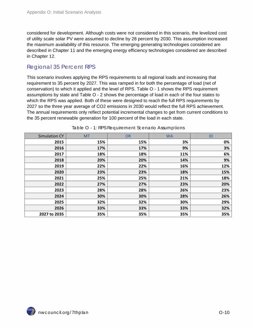
Appendix O: Initial Scenario Analysis
nwcouncil.org/7thplan O-10
considered for development. Although costs were not considered in this scenario, the levelized cost of utility scale solar PV were assumed to decline by 28 percent by 2030. This assumption increased the maximum availability of this resource. The emerging generating technologies considered are described in Chapter 11 and the emerging energy efficiency technologies considered are described in Chapter 12.
Regional 35 Percent RPS
This scenario involves applying the RPS requirements to all regional loads and increasing that requirement to 35 percent by 2027. This was ramped in for both the percentage of load (net of conservation) to which it applied and the level of RPS. Table O - 1 shows the RPS requirement assumptions by state and Table O - 2 shows the percentage of load in each of the four states to which the RPS was applied. Both of these were designed to reach the full RPS requirements by 2027 so the three year average of CO2 emissions in 2030 would reflect the full RPS achievement. The annual requirements only reflect potential incremental changes to get from current conditions to the 35 percent renewable generation for 100 percent of the load in each state.
Table O - 1: RPS Requirement Scenario Assumptions
Simulation CY MT OR WA ID 2015 15% 15% 3% 0% 2016 17% 17% 9% 3% 2017 18% 18% 11% 6% 2018 20% 20% 14% 9% 2019 22% 22% 16% 12% 2020 23% 23% 18% 15% 2021 25% 25% 21% 18% 2022 27% 27% 23% 20% 2023 28% 28% 26% 23% 2024 30% 30% 28% 26% 2025 32% 32% 30% 29% 2026 33% 33% 33% 32%
2027 to 2035 35% 35% 35% 35%

Appendix O: Initial Scenario Analysis
nwcouncil.org/7thplan O-11
Table O - 2: Percent of Obligated Load Assumptions
Simulation CY MT OR WA ID 2015 56% 71% 76% 0% 2016 60% 73% 78% 8% 2017 63% 76% 80% 17% 2018 67% 78% 82% 25% 2019 71% 81% 84% 33% 2020 74% 83% 86% 42% 2021 78% 86% 88% 50% 2022 82% 88% 90% 58% 2023 85% 90% 92% 67% 2024 89% 93% 94% 75% 2025 93% 95% 96% 83% 2026 96% 98% 98% 92%
2027 to 2035 100% 100% 100% 100%
No Demand Response - No Carbon Cost
For this scenario, the resource strategies were restricted so that they could not select demand response resources as options. For a description of the optioning logic in the RPM see the earlier section in this chapter on estimating the cost of new generating resources and demand response.
Low Fuel and Market Prices - No Carbon Cost
This scenario explores the implications of extremely low natural gas prices and the corresponding impacts on other fuel and electricity prices. This includes a reduction in coal prices, for example the price for coal in Montana start around $0.03 less per MMBTU in this scenario and by 2035 are around $0.17 less in real 2012 dollars. The range of natural gas prices is based on re-centering the prices around the low forecast range as described in Chapter 8. The resulting range of natural gas prices can be seen in Figure O - 3. The electricity prices used in examining the resource strategies under this scenario are then centered around an electricity price forecast based on this low natural gas price forecast and the resulting range of electricity prices for importing or exporting power generation can be seen in Figure O - 4.

Appendix O: Initial Scenario Analysis
nwcouncil.org/7thplan O-12
Figure O - 3: Range of Natural Gas Prices

Appendix O: Initial Scenario Analysis
nwcouncil.org/7thplan O-13
Figure O - 4: Range of Electricity Prices
No Coal Retirement
In this scenario, the announced retirements of the Boardman, Centralia and North Valmy resources was taken out of the model. This was used to determine the impacts of these retirements on the resource strategy.
Lower Conservation - No Carbon Cost
In this scenario, the resource strategy was limited so that conservation could only be purchased if its cost was anticipated to be at or below short-run market prices. These same restrictions were not applied to other resources. This scenario is useful in examining the cost of this conservation purchasing scheme compared to developing conservation at a level that minimizes future power system costs where it is purchased on an equivalent basis to other resources.
Scenarios with Carbon Costs Social Cost of Carbon - Mid-Range and High-Range
These scenarios assumed that alternate values of the federal government’s estimates1 for damage caused to society by climate change resulting from carbon dioxide emissions, referred to as the Social Cost of Carbon, are imposed beginning in 2016. The mid-range scenario used the average cost estimated with a 3 percent discount rate. The high-range scenario used an estimate of possible
1 Estimated cost of the damage of carbon emissions by the Interagency Working Group on Social Cost of Carbon

Appendix O: Initial Scenario Analysis
nwcouncil.org/7thplan O-14
damage cost that should not occur more than 5 percent of the time. Values for these scenarios are given in Table O - 3.
By internalizing carbon costs, this analysis identifies strategies that minimize all costs, including carbon.
The model essentially reduces carbon emissions when they can be avoided at the social cost of carbon or less. The policy basis for these scenarios is that the cost of resource strategies developed under conditions which fully internalized the damage cost from carbon emissions would be the maximum society should invest to avoid such damage.
Table O - 3: Social Cost of Carbon Assumptions (2012$/Metric Ton of CO2)
Fiscal Year Mid-Range High-Range FY16 $40.99 $121.00 FY17 $42.07 $125.00 FY18 $43.15 $129.00 FY19 $45.31 $134.00 FY20 $46.39 $138.00 FY21 $46.39 $141.00 FY22 $47.47 $145.00 FY23 $48.54 $148.00 FY24 $49.62 $151.00 FY25 $50.70 $154.00 FY26 $51.78 $158.00 FY27 $52.86 $161.00 FY28 $53.94 $164.00 FY29 $55.02 $167.00 FY30 $56.10 $172.00 FY31 $56.10 $175.00 FY32 $57.17 $178.00 FY33 $58.25 $181.00 FY34 $59.33 $186.00 FY35 $60.41 $189.00
Carbon Cost Risk
In this scenario, the price associated with CO2 per metric ton was modeled as a regulatory risk. The range of the potential carbon price was fixed between $0 and $110 in real 2012 dollars. The price can be applied starting from 2015 through 2035. Uncertainty about the starting date of the potential CO2 price makes this pricing scheme more consistent with an explicit price for CO2. This scenario was consistent with the CO2 risk scenario analyzed in the Sixth Power Plan and allows for some comparison between plans. More detail on the CO2 risk model is included in Appendix L.

Appendix O: Initial Scenario Analysis
nwcouncil.org/7thplan O-15
Resource Uncertainty – Planned and Unplanned Loss of a Major Resource
Two scenarios were run to examine the impacts of resource uncertainty. In the first scenario non-CO2 emitting resources were retired in 2016, 2019, 2022 and 2025 for a combined total of about 1,000 megawatts nameplate. The other scenario involved a single similarly sized non-CO2 emitting resource, which was randomly shut down or retired sometime between 2016 and 2035. This was done using a uniform probability of retirement during each quarter.
Faster and Slower Conservation Deployment
These scenarios involved changing the input assumptions for maximum achievable conservation per year. Chapter 12 discusses the development of the input assumptions for faster and slower ramping of conservation programs. For a more detailed description of how the maximum available conservation per year, the percent of that conservation that can be achieved by program year and the maximum conservation that can be achieved over the 20-year study period see Appendix L.
No Demand Response – Carbon Cost
This scenario is the same as the No Demand Response - No Carbon Cost scenario except that it includes the carbon prices from the Social Cost of Carbon - Mid-Range scenario.
Low Fuel and Market Prices – Carbon Cost
This scenario is the same as the Low Fuel and Market Prices - No Carbon Cost scenario except that it includes the carbon prices from the Social Cost of Carbon - Mid-Range scenario.
Increased Reliance on External Markets
One of the RPM’s input assumptions is the maximum level of reliance on out-of-region markets permitted to meet regional adequacy standards. In this scenario, this assumption was relaxed, i.e., reliance on out-of-region markets was increased. To implement this, the GENESYS model was run to determine the Adequacy Reserve Margins (ARM) under the assumption that maximum market reliance is 3,400 MW during high load hours in the winter instead of 2500 MW during high load hours in the winter currently used in the Resource Adequacy Assessment.2 Since the ARM is a “reserve margin” over in-region utility controlled resources, the assumption of greater external market reliance lowers the ARM requirements. The ARM values were recalculated with a higher expectation of import availability. The result of this is that fewer in-region resources are required to be built for capacity. While the ARM for energy is roughly the same in this scenario at around -3.0 percent, the ARM for capacity is reduced from around 3.0 percent to almost -1.0 percent.
2 The basis of and methodology used to develop the Adequacy Reserve Margins are described in Chapter 11.
Appendix O: Initial Scenario Analysis
nwcouncil.org/7thplan O-16
EXAMINING RESULTS The resource strategy of the Seventh Power Plan is designed to provide the region a low-cost electricity supply to meet future load growth. It is also designed to provide a low economic risk electricity future by ensuring that the region develops and controls sufficient resources to maintain resource adequacy, limiting exposure to potential market price extremes. Therefore the amount and type of resources included in the strategy are designed to meet loads, minimize costs, and help reduce the economic risks posed by uncertain future events.
Figure O - 5 shows the average resource development by resource type for the least cost resource strategy under the major scenarios and sensitivity studies carried out to support the development of the Seventh Power Plan. The resource development shown in Figure O - 5 is the average over all 800 futures modeled in the Regional Portfolio Model (RPM). In the RPM the specific timing and level of resource development is unique to each of the 800 potential futures modeled. The Seventh Power Plan’s principal of adaptive management is based on the reality that, as in the RPM, the timing and level of resource development in the region will be determined by actual conditions as they unfold over the next 20 years. However, what should not change are the Seventh Power Plan’s priorities for resource development. In that regard, Figure O - 5 shows the significant and consistent role of energy efficiency across all scenarios. This is because of its low cost, its contribution to regional winter capacity needs and its role in mitigating economic risk from fuel price uncertainty and volatility.
After energy efficiency, the average development of new natural gas generation and renewable resources by 2035 is roughly equivalent. New natural gas-fired resources are developed to meet regional capacity needs while renewable resource development is driven by state renewable resource portfolio standards. Not shown in Figure O - 5 is the deployment of demand response resources because these resources primarily provide capacity (megawatts) not energy (average megawatts) and the increased dispatch of existing gas generation to replace retiring coal generation. Both of these resources also play significant roles in the Seventh Power Plan’s resource strategy. Each element of the resource strategy is discussed below.

Appendix O: Initial Scenario Analysis
nwcouncil.org/7thplan O-17
Figure O - 5: Average Resource Development in Least Cost Resource Strategy by 2035 in Alternative Scenarios
Energy Efficiency Resources Energy efficiency has been important in all previous Council power plans. The region has a long history of experience improving the efficiency of electricity use. Since the Northwest Power Act was enacted, the region has developed nearly 5,800 average megawatts of conservation. This achievement makes efficiency the second-largest source of electricity in the region following hydroelectricity.
As in all prior plans, the highest priority new resource in the Seventh Power Plan resource strategy is improved efficiency of electricity use, or conservation. Figure O - 6 shows that the region’s net load after development of all-cost effective energy efficiency remains essentially the same over the next 20 years. This finding holds under scenarios that both consider carbon dioxide risk or damage cost and those that do not and even when natural gas and electricity prices are lower than generally anticipated. The only scenario that developed significantly less energy efficiency was the scenario specifically designed to do so. The Lower Conservation scenario developed roughly 1200 average megawatts less energy efficiency by 2035 than the Existing Policy scenario. The Lower Conservation scenario had significantly higher ($14 billion) average system cost and exposed the region to much larger ($19 billion) economic risk than the Existing Policy scenario. However, as Figure 3 - 2 shows, even under that scenario, the development of energy efficiency offsets regional load growth through 2030.
The attractiveness of improved efficiency is due to its relatively low cost coupled with the fact that it provides both energy and capacity savings and is not subject to major sources of economic risk. The
- 1,000 2,000 3,000 4,000 5,000
SCC - High Unplanned Loss of Major Resource
SCC - Mid-Range Faster Conservation Deployment
Planned Loss of Major Resource No Demand Response
Carbon Cost Risk Slower Conservation Deployment
No Demand Response - Carbon Risk Maximum Carbon Reduction - Existing Technology
Existing Policy Low Gas Prices - Carbon Risk
Increased Market Reliance RPS at 35%
Low Gas Prices Lower Conservation
Average Resource Development by 2035 (aMW) New Gas Development
Renewable Development
Conservation Development

Appendix O: Initial Scenario Analysis
nwcouncil.org/7thplan O-18
average cost of conservation developed in the least cost resource strategies across all scenarios tested was half the cost of alternative generating resources. The average levelized cost of the cost-effective efficiency developed in the Seventh Power Plan’s resource strategy is $30 per megawatt-hour.3 The comparable estimated cost of a natural gas-fired combined-cycle combustion turbine is around $75 per megawatt-hour. The current cost of utility scale solar photovoltaic systems is approximately $65 per megawatt-hour and Columbia Basin wind costs $110 per megawatt-hour, including the cost of integrating these variable output resources into the power system. Significant amounts of improved efficiency also cost less than the forecast market price of electricity. Nearly 2,300 average megawatts of energy efficiency are available at cost below $30 per megawatt-hour.
Conservation also lacks the economic risk associated with volatile fuel prices and carbon dioxide emission reduction policies. Its short lead time and availability in small increments also reduce its economic risk. Therefore, improved efficiency reduces both the cost and economic risk of the Seventh Power Plan’s resource strategy.
Figure O - 6: Average Net Regional Load After Accounting for Cost-Effective Conservation Resource Development
3 This is the average real levelized cost of all conservation measures acquired in the resource strategy, excluding a cost-offset that is expected to occur as a result of lower load growth which defers the need to expand distribution and transmission systems. In evaluating conservation’s cost-effectiveness in the RPM, this cost-offset was included, as well as other non-energy benefits, such as water savings from more efficient clothes washers. If the cost-offset benefits provided by energy efficiency’s deferral of investments in distribution and transmission expansion are considered, the average levelized cost is $18 per megawatt-hour.
10,000
12,000
14,000
16,000
18,000
20,000
22,000
24,000
2016 2019 2022 2025 2028 2031 2034
Annu
al N
et L
oad
(aM
W)
Existing Policy
Carbon Cost Risk
Low Gas Prices
Lower Conservation

Appendix O: Initial Scenario Analysis
nwcouncil.org/7thplan O-19
In the Council’s analysis, additional resources are added to provide insurance against future uncertainties. Efficiency improvement provides attractive insurance for this purpose because of its low cost. In futures or time periods when the extra resources are not immediately needed, the energy and capacity can be sold in the market and all or at least a portion of their cost recovered. This is not true for generating resources, for in periods when market prices are at or below their variable operating cost; these resources cannot recover any of their capital cost. In addition, because of its low average cost to utilities, the development of energy efficiency offers the potential opportunity to extend the benefits of the Northwest’s hydro-system through increased sales.
In all of the scenarios and sensitivity studies examined by the Council, similar amounts of improved efficiency were found to be cost-effective.4 The selection of energy efficiency as the primary new resource does not depend significantly on whether or not carbon dioxide policies are enacted. Figure O - 7 shows the average amount of efficiency acquired in various scenarios considered by the Council in the power plan by 2021, 2026, and 2035. In all scenarios, the amount of cost-effective efficiency developed averages between 1,300 and 1,450 average megawatts by 2021 and 3,900 and 4,600 by 2035. The amount of conservation developed varies in each future considered in the Regional Portfolio Model. For example, in the Carbon Cost Risk scenario, the average conservation development is 4,485 average megawatts, but individual futures can vary from as low as 4,000 average megawatts to as high as just over 5,000 average megawatts.
4 The only exception is the Lower Conservation scenario which as explicitly designed to develop less energy efficiency.

Appendix O: Initial Scenario Analysis
nwcouncil.org/7thplan O-20
Figure O - 7: Amount of Cost-Effective Conservation Resources Developed Under Different Scenarios
The nature of efficiency improvement is that the total cost is recovered over a smaller number of sales. Average cost per kilowatt-hour sold will increase, but because total consumption is reduced, average consumer electricity bills will be smaller. Consumers who choose not to improve their efficiency of use could see their bills increase. However, if the region does not capture the efficiency, the higher cost of other new generating resources will increase everyone’s bills. The impact on both bills and average revenue requirement per kilowatt-hour is discussed later in this chapter.
The Council has identified significant new efficiency opportunities in all consuming sectors. Figure O - 8 shows by levelized cost the sectors of efficiency improvements. Additional information on the sources and costs of efficiency improvements is provided in Chapter 12 and Appendix G.
Improved efficiency contributes not only to meeting future energy requirements, but also provides capacity during peak load periods. The savings from conservation generally follow the hourly shape of energy use, saving more energy when more is being used. As a result, efficiency contributes more to load reduction during times of peak usage. To model the impact of energy efficiency on the hourly demand for electricity, the Council aggregated the load shapes of efficiency savings from the hourly shape of individual end-uses of electricity and the cost-effective efficiency improvements in those uses. Figure O - 9 shows the shape of the savings for all measures during heavy and light load hours. As is shown, the energy savings are greater during the winter season than summer, in large part due to significant savings from conversion of electric resistance heating to more efficient heat pump technologies and increased use of lighting during the winter period.
- 500
1,000 1,500 2,000 2,500 3,000 3,500 4,000 4,500 5,000
SCC
- Hig
h
Unp
lann
ed L
oss o
f Maj
or R
esou
rce
SCC
- Mid
-Ran
ge
Fast
er C
onse
rvat
ion
Depl
oym
ent
Plan
ned
Loss
of M
ajor
Res
ourc
e
No
Dem
and
Resp
onse
Carb
on C
ost R
isk
Slow
er C
onse
rvat
ion
Depl
oym
ent
No
Dem
and
Resp
onse
- Ca
rbon
Cos
t Ri
sk
Max
imum
CO
2 Re
duct
ion
- Exi
stin
g Te
chno
logy
Exist
ing
Polic
y
Low
Gas
Pric
es -
Carb
on C
ost R
isk
Incr
ease
d M
arke
t Rel
ianc
e
RPS
at 3
5%
Low
Gas
Pric
es
Low
er C
onse
rvat
ion
Aver
age
Cons
erva
tion
Deve
lopm
ent
by
2035
(aM
W)
2021 2026 2035

Appendix O: Initial Scenario Analysis
nwcouncil.org/7thplan O-21
Figure O - 8: Efficiency Potential by Sector and Levelized Cost by 2035
For example, efficiency improvements that yield average annual savings of 4,485 average megawatts create 10,700 megawatts of peak hour savings during the winter months.5 The capacity impact of energy efficiency is almost two times the energy contribution in winter. This reduction in both system energy and capacity needs makes energy efficiency a valuable resource relative to generation because efficiency provides winter energy and capacity resources shaped to load. Because each efficiency measure has a specific shape, or capacity impact, the Seventh Power Plan explicitly incorporates the value of deferred generation capacity in the cost-effectiveness methodology for measures and programs.6
5 See Chapter 12 for a description of how the capacity savings of energy efficiency measures are estimated and Chapter 11 for a description of how the system level capacity savings, or Associated System Capacity Contributions, of conservation and generation resources are estimated. 6 See action items RES-2 and RES-3 in Chapter 4 and Appendix G
-
1,000
2,000
3,000
4,000
5,000
6,000
<0 <10 <20 <30 <40 <50 <60 <70 <80 <90 <100 <110 <120 <130 <140 >140
Reso
urce
Pot
entia
l (aM
W)
Real Levelized Cost (2012$/MWh)
Agriculture Commercial Industrial Residential Utility
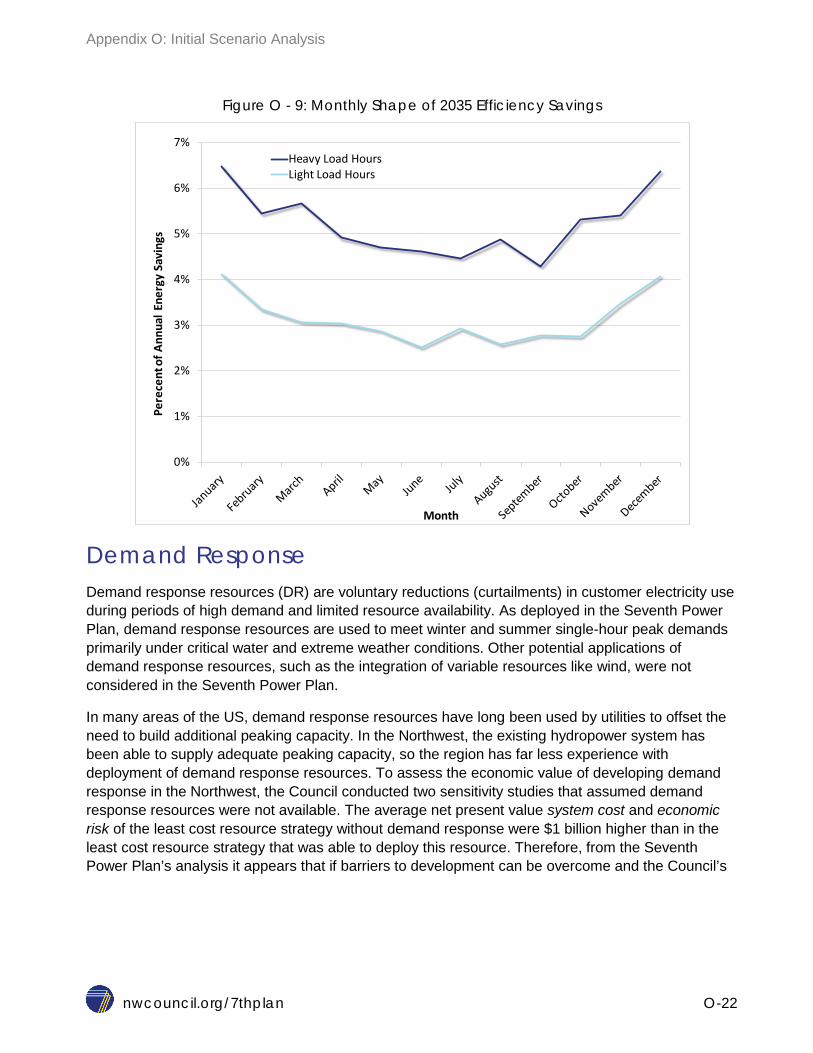
Appendix O: Initial Scenario Analysis
nwcouncil.org/7thplan O-22
Figure O - 9: Monthly Shape of 2035 Efficiency Savings
Demand Response Demand response resources (DR) are voluntary reductions (curtailments) in customer electricity use during periods of high demand and limited resource availability. As deployed in the Seventh Power Plan, demand response resources are used to meet winter and summer single-hour peak demands primarily under critical water and extreme weather conditions. Other potential applications of demand response resources, such as the integration of variable resources like wind, were not considered in the Seventh Power Plan.
In many areas of the US, demand response resources have long been used by utilities to offset the need to build additional peaking capacity. In the Northwest, the existing hydropower system has been able to supply adequate peaking capacity, so the region has far less experience with deployment of demand response resources. To assess the economic value of developing demand response in the Northwest, the Council conducted two sensitivity studies that assumed demand response resources were not available. The average net present value system cost and economic risk of the least cost resource strategy without demand response were $1 billion higher than in the least cost resource strategy that was able to deploy this resource. Therefore, from the Seventh Power Plan’s analysis it appears that if barriers to development can be overcome and the Council’s
0%
1%
2%
3%
4%
5%
6%
7%Pe
rece
nt o
f Ann
ual E
nerg
y Sa
ving
s
Month
Heavy Load HoursLight Load Hours

Appendix O: Initial Scenario Analysis
nwcouncil.org/7thplan O-23
analysis of the cost of demand response are accurate; demand response resources could provide significant regional economic benefits.7
The Council’s assessment identified more than 4300 megawatts of regional demand response potential. A significant amount of this potential, more than 1500 megawatts, is available at relatively low cost, under $25 per kilowatt of peak capacity per year. When compared to the alternative of constructing a simple cycle gas-fired turbine, demand response resources can be deployed sooner and in quantities better matched to the peak capacity need. Figure O - 10 shows the cumulative potential for each of the four blocks (i.e., price bins) of demand response modeled in the Regional Portfolio Model. Cumulative achievable potential by the years 2021, 2026, and 2035 is shown for both winter and summer capacity demand response programs. Note that the largest single block of estimated demand response potential is also the least costly.
Figure O - 10: Demand Response Resource Supply Curve
The low cost of demand response resources make them the most economically attractive option for maintaining regional peak reserves to satisfy the Council’s Resource Adequacy Standards. The low cost of demand response resources make them particularly valuable because the need for peaking capacity resources to meet resource adequacy in the region is a function of a combination of water and weather conditions that have low probability of occurrence. This is illustrated by Figure O - 11 which shows the amount of demand response resource needed by 2021 across the 800 futures tested in the RPM across multiple scenarios.
7 See Chapter 4 for the Action Items the Seventh Power Plan recommends the region and Bonneville should engage to specifically address the barriers to development of demand response resources.
0
200
400
600
800
1000
1200
1400
1600
1800
$25 $54 $77 $189
Cum
ulat
ive
Pot
entia
l (M
W)
Demand Response Price Bins (2012$ per kW-year)
2021 Winter 2026 Winter
2035 Winter 2021 Summer
2026 Summer 2035 Summer
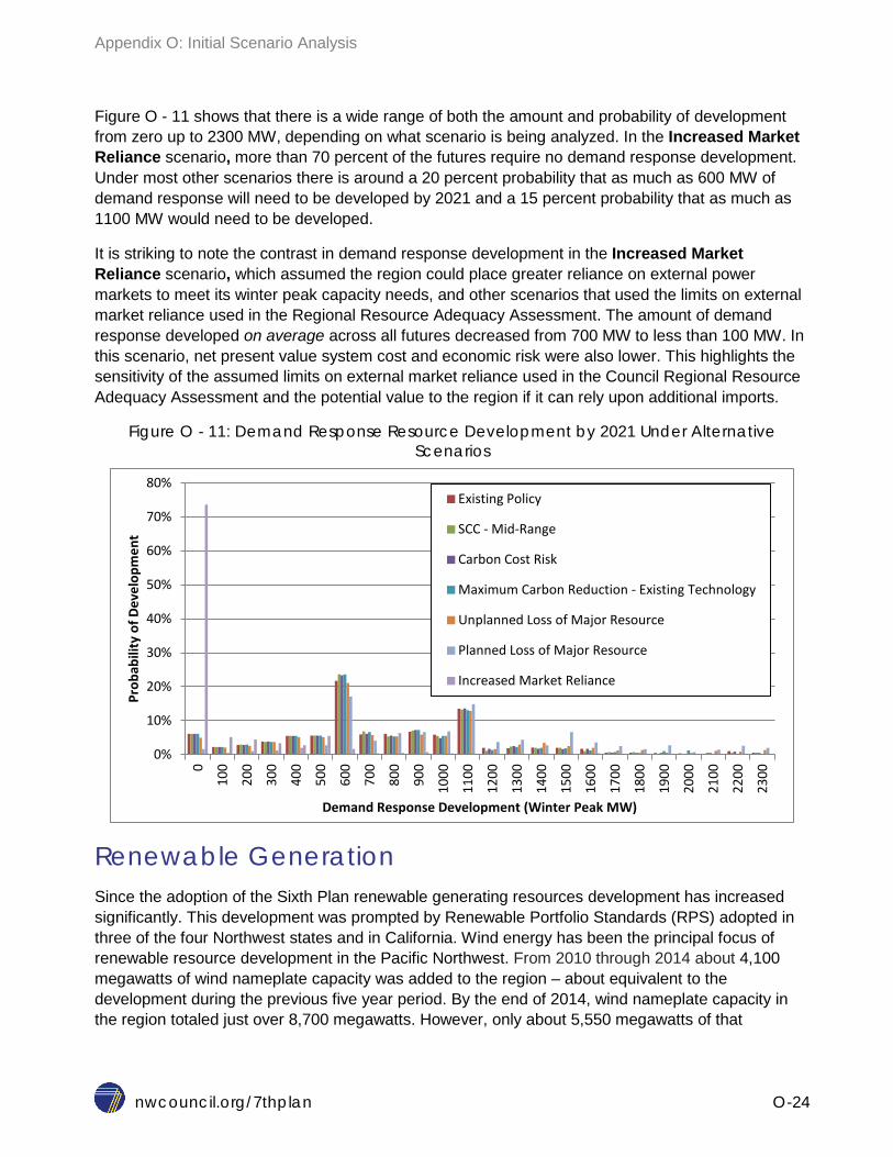
Appendix O: Initial Scenario Analysis
nwcouncil.org/7thplan O-24
Figure O - 11 shows that there is a wide range of both the amount and probability of development from zero up to 2300 MW, depending on what scenario is being analyzed. In the Increased Market Reliance scenario, more than 70 percent of the futures require no demand response development. Under most other scenarios there is around a 20 percent probability that as much as 600 MW of demand response will need to be developed by 2021 and a 15 percent probability that as much as 1100 MW would need to be developed.
It is striking to note the contrast in demand response development in the Increased Market Reliance scenario, which assumed the region could place greater reliance on external power markets to meet its winter peak capacity needs, and other scenarios that used the limits on external market reliance used in the Regional Resource Adequacy Assessment. The amount of demand response developed on average across all futures decreased from 700 MW to less than 100 MW. In this scenario, net present value system cost and economic risk were also lower. This highlights the sensitivity of the assumed limits on external market reliance used in the Council Regional Resource Adequacy Assessment and the potential value to the region if it can rely upon additional imports.
Figure O - 11: Demand Response Resource Development by 2021 Under Alternative Scenarios
Renewable Generation Since the adoption of the Sixth Plan renewable generating resources development has increased significantly. This development was prompted by Renewable Portfolio Standards (RPS) adopted in three of the four Northwest states and in California. Wind energy has been the principal focus of renewable resource development in the Pacific Northwest. From 2010 through 2014 about 4,100 megawatts of wind nameplate capacity was added to the region – about equivalent to the development during the previous five year period. By the end of 2014, wind nameplate capacity in the region totaled just over 8,700 megawatts. However, only about 5,550 megawatts of that
0%
10%
20%
30%
40%
50%
60%
70%
80%
0
100
200
300
400
500
600
700
800
900
1000
1100
1200
1300
1400
1500
1600
1700
1800
1900
2000
2100
2200
2300
Prob
abili
ty o
f Dev
elop
men
t
Demand Response Development (Winter Peak MW)
Existing Policy
SCC - Mid-Range
Carbon Cost Risk
Maximum Carbon Reduction - Existing Technology
Unplanned Loss of Major Resource
Planned Loss of Major Resource
Increased Market Reliance

Appendix O: Initial Scenario Analysis
nwcouncil.org/7thplan O-25
nameplate capacity currently serves Northwest loads. The remaining 3,150 megawatts of wind nameplate capacity is presently contracted to utilities outside the region, primarily California.
It appears, however, that the rapid development of wind is likely to slow down over the next five year period due to the expiration of incentives and low load growth.
Existing wind resources are estimated to provide about 2,400 average megawatts of energy generation per year in the region, or about 8 percent of the region’s electricity energy supply. However, on a firm capacity basis, wind resources only provide about 1 percent of the region’s total system peaking capability. The Council’s current analysis of wind’s ability to supply peaking capacity is based on the Resource Adequacy Assessment Advisory Committee’s estimate that wind can only be relied upon to provide about 5 percent of its nameplate capacity toward meeting peak loads due to the variable nature of the resource.
Aside from hydropower, the renewable resources included in the Regional Portfolio Model (RPM) are wind and solar photovoltaic (solar PV). The Council recognizes that additional small-scale renewable resources are likely available and cost-effective. These small-scale renewables were not modeled in the RPM but the plan encourages their development as an important element of the resource strategy. In addition, there are many potential renewable resources not captured in the resource strategy that are currently either too expensive or unproven technologies that may, with additional research and demonstration, prove to be valuable future resources.
New wind resources that have ready access to transmission produce energy at costs that are competitive on an energy basis with other generation alternatives. Recent and forecast reductions in solar PV system cost are making utility scale system’s energy production cost increasingly cost-competitive. However, renewable generation development in the scenarios tested for the Seventh Power Plan is driven by state RPS and not economics. Figure O - 12 shows the average development of renewable resources across scenarios analyzed for the Seventh Power Plan. As can be seen from this figure, under all least cost resource strategies for all scenarios, except when the RPS were assume to increase to 35 percent, only 300 to 400 average megawatts of renewable resource development occurs later in the planning period (post-2026) after the Oregon and Washington renewable credit bank balances are forecast to be drawn down.

Appendix O: Initial Scenario Analysis
nwcouncil.org/7thplan O-26
Figure O - 12: Average Renewable Resource Development by Scenarios by 2021, 2026 and 2035
The amount of renewable energy acquired depends on the future demand for electricity because state requirements specify percentages of demand that have to be met with qualifying renewable sources of energy. Across the 800 futures of demand growth in the Carbon Cost Risk scenario, the amount of wind and solar PV developed on average is about 300 average megawatts, with slightly more solar PV developed than wind. The only exception to this level of development is the RPS at 35 percent scenario that assumed regional renewable resource portfolio standards would be increased to 35 percent of annual regional load. In this scenario the least cost resource strategy develops 2,900 average megawatts of additional renewable resources, primarily wind generation by 2035.
The explanation of the outcome described above is that while the two economically competitive renewable resources available in the region, wind and solar PV, produce significant amounts of energy, they provide little or no winter peaking capacity. Partly as a result of the significant wind development in the region over the past decade, the Northwest has a significant energy surplus, yet under critical water and extreme weather conditions the region faces the probability of a winter peak capacity shortfall. In short, the generation characteristics of the currently economically competitive renewable resources do not align well with regional power system needs.
As stated above, the development of renewable generation is driven by state renewable portfolio standards more so than regional energy need. In the absence of higher renewable portfolio standards little additional renewable development would take place, even under scenarios where the highest social cost of carbon dioxide (SCC-High) might be imposed on the power system.
-
500
1,000
1,500
2,000
2,500
3,000
3,500
2021 2026 2035
Aver
age
Annu
al G
ener
atio
n (a
MW
)
RPS at 35%
SCC - High
Low Gas Prices - Carbon Cost Risk
Existing Policy
Maximum Carbon Reduction - Existing Technology No Demand Response - Carbon Cost Risk
Slower Conservation Deployment
No Demand Response
SCC - Mid-Range
Faster Conservation Deployment

Appendix O: Initial Scenario Analysis
nwcouncil.org/7thplan O-27
Natural Gas-Fired Generation Natural gas is the fourth major element in the Seventh Power Plan resource strategy. It is clear that after efficiency and demand response, new natural gas-fired generation is the most cost-effective resource option for the region in the near-term. Moreover, also after energy efficiency, the Seventh Power Plan identified the increased use of existing natural gas generation as offering the lowest cost option for reducing regional carbon dioxide emissions. Other resource alternatives may become available over time, and the Seventh Power Plan recommends actions to encourage expansion of the diversity of resources available, especially those that do not produce greenhouse gas emissions.
Across the scenarios evaluated, there is significant variance in the amount of new gas-fired generating resources that are optioned and in the likelihood of completing the plants. New gas-fired plants are optioned (sited and licensed) in the RPM so that they are available to develop if needed in each future. The Seventh Power Plan’s resource strategy includes optioning new gas fired generation as local needs dictate. However, from an aggregate regional perspective, which is the plan’s focus, the need for additional new natural gas-fired generation is very limited in the near term (through 2021) and low in the mid-term (through 2026) under nearly all scenarios. That is, options for new gas-fired generation are taken to construction in only a relatively small number of futures. Figures 15 - 17 and 15 - 18 show the probability that a thermal resource option would move to construction by 2021 and by 2026. The scenarios are rank-ordered based on the probability of any new gas resource development by 2021 and by 2026. Scenarios with the lowest probability of development are at the top of the graphs.
As can be observed from a review of Figure O - 13, the probability of gas development is less than 10 percent by 2021 in all but four scenarios. The only exceptions to this finding are in the RPS at 35 percent scenario and in scenarios where the region is unable to deploy demand response or acquires less conservation than projected. In these scenarios, the probability of moving from an option to construction on new gas-fired generation increases to 40 percent or higher.
By 2026, Figure O - 14 shows that the probability of moving from an option to actual construction of a new gas-fired thermal plant increases to more than 80 percent in the SCC-High and Maximum Carbon Reduction – Existing Technology scenarios. This occurs because under both of these scenarios existing coal and inefficient gas-fired generation are retired or displaced by new, highly efficient natural gas generation to reduce regional carbon dioxide emissions.
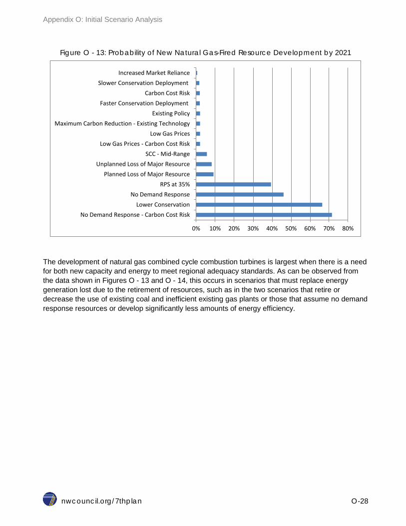
Appendix O: Initial Scenario Analysis
nwcouncil.org/7thplan O-28
Figure O - 13: Probability of New Natural Gas-Fired Resource Development by 2021
The development of natural gas combined cycle combustion turbines is largest when there is a need for both new capacity and energy to meet regional adequacy standards. As can be observed from the data shown in Figures O - 13 and O - 14, this occurs in scenarios that must replace energy generation lost due to the retirement of resources, such as in the two scenarios that retire or decrease the use of existing coal and inefficient existing gas plants or those that assume no demand response resources or develop significantly less amounts of energy efficiency.
0% 10% 20% 30% 40% 50% 60% 70% 80%
No Demand Response - Carbon Cost Risk Lower Conservation
No Demand Response RPS at 35%
Planned Loss of Major Resource Unplanned Loss of Major Resource
SCC - Mid-Range Low Gas Prices - Carbon Cost Risk
Low Gas Prices Maximum Carbon Reduction - Existing Technology
Existing Policy Faster Conservation Deployment
Carbon Cost Risk Slower Conservation Deployment
Increased Market Reliance

Appendix O: Initial Scenario Analysis
nwcouncil.org/7thplan O-29
Figure O - 14: Probability of New Natural Gas-Fired Resource Development by 2026
As can be seen from the prior discussion, while the amounts of efficiency, demand response, and renewable resources developed were fairly consistent across most scenarios examined, the future role of new natural gas-fired generation is more variable and specific to the scenarios studied. Figure O - 15 shows the average amounts of gas-fired generation across 800 futures considered in each of the principal scenarios. The amount of new natural gas-fired generation constructed varies in each future. In most scenarios the average annual dispatch of new natural gas-fired generation is less than 50 average megawatts by 2026 and only between 300 to 400 average megawatts by 2035. In the Carbon Cost Risk scenario, the amount of energy generated from new combined cycle combustion turbines, when averaged across all 800 futures examined, is just 10 average megawatts in 2035. In contrast, the average amount generated across 800 futures is closer to 100 average megawatts in 2035 in the two scenarios that assume no demand response resources are developed.
However, the role of natural gas is larger than it appears in the Council’s analysis of the regional need for new natural gas fired generation for a number of reasons. First, the regional transmission system has not evolved as rapidly as the electricity market, resulting in limited access to market power for some utilities. Second, some utilities have significant near-term resource challenges, particularly if there is limited access to surplus resources from others. These factors limit the ability of the regional resource strategy to be specific about optioning and construction dates for natural gas-fired resources, or for the types of natural gas-fired generation. As a result, new gas-fired generation may be required in such instances even if the utilities deploy demand response resources and develop the conservation as called for in Seventh Power Plan.
0% 10% 20% 30% 40% 50% 60% 70% 80% 90% 100%
Maximum Carbon Reduction - Existing Technology SCC - High
Lower Conservation No Demand Response - Carbon Cost Risk
No Demand Response Planned Loss of Major Resource
Unplanned Loss of Major Resource SCC - Mid-Range
Low Gas Prices - Carbon Cost Risk Faster Conservation Deployment
Carbon Cost Risk Slower Conservation Deployment
Low Gas Prices Existing Policy
RPS at 35% Increased Market Reliance

Appendix O: Initial Scenario Analysis
nwcouncil.org/7thplan O-30
Figure O - 15: Average New Natural Gas-Fired Resource Development
Third, the increased use of the existing natural gas generation in the region plays a major role in many of scenario’s least cost resource strategies, particularly those that explored alternative carbon dioxide emissions reduction policies. Figure O - 16 shows the average annual dispatch of the existing natural gas generation in the region through time for the five carbon dioxide reduction policy scenarios as well as the Existing Policy scenario. A review of Figure O - 16 reveals that the annual dispatch of existing natural gas generating resources increases in response to carbon dioxide emission reduction policies.
For example, under the two Social Cost of Carbon scenarios, existing natural gas generation increases immediately following the assumed 2016 imposition of carbon dioxide damage cost in those scenarios. In the Carbon Cost Risk scenario, existing natural gas generation gradually increases over time as the regulatory cost of carbon dioxide increases. In the Maximum Carbon Reduction – Existing Technology scenario, existing gas generation increases post-2025 when, under this scenario, the entire region’s existing coal-fired generation fleet is retired. Under the RPS at 35 percent scenario, existing natural gas generation actually declines through time as low variable cost resources are added to the system, generally lowering market prices and diminishing the economics of gas dispatch.
-
500
1,000
1,500
2,000
2021 2026 2035
Aver
age
Annu
al G
ener
atio
n (a
MW
)
RPS at 35% Existing Policy Increased Market Reliance No Demand Response Low Gas Prices Slower Conservation Deployment Faster Conservation Deployment Carbon Cost Risk SCC - Mid-Range Low Gas Prices - Carbon Cost Risk No Demand Response - Carbon Cost Risk Planned Loss of Major Resource Unplanned Loss of Major Resource Lower Conservation Maximum Carbon Reduction - Existing Technology

Appendix O: Initial Scenario Analysis
nwcouncil.org/7thplan O-31
Figure O - 16: Average Annual Dispatch of Existing Natural Gas-Fired Resources
Carbon Emissions As in the Sixth Power Plan, one of the key issues identified for the Seventh Power Plan is climate-change policy and the potential effects of proposed carbon regulations. In addition, the Council was asked to address what changes would be needed to the power system to reach a specific carbon reduction goal and what those changes would cost. This section summarizes how alternative resource strategies compare with respect to their cost and ability to meet carbon dioxide emissions limits established by the Environmental Protection Agency. In providing analysis of carbon emissions and the specific cost of attaining carbon emission limits, the Council is not taking a position on future climate-change policy. Nor is the Council taking a position on how individual Northwest states or the region should comply with EPA’s carbon dioxide emission regulations. The Council’s analysis is intended to provide useful information to policy-makers.
Figure O - 17 shows the two U.S. Government Interagency Working Group’s estimates used for the two Social Cost of Carbon scenarios and the range (shaded area) and average carbon prices across all futures that were evaluated in the $0-to-$110-per-metric ton Carbon Risk scenario.
-
500
1,000
1,500
2,000
2,500
3,000
3,500
4,000
4,500
2015 2020 2025 2030 2035
Aver
age
Annu
al D
ispa
tch
(aM
W)
Existing Policy SCC - Mid-Range SCC - High Carbon Cost Risk Maximum Carbon Reduction - Existing Technology RPS at 35%
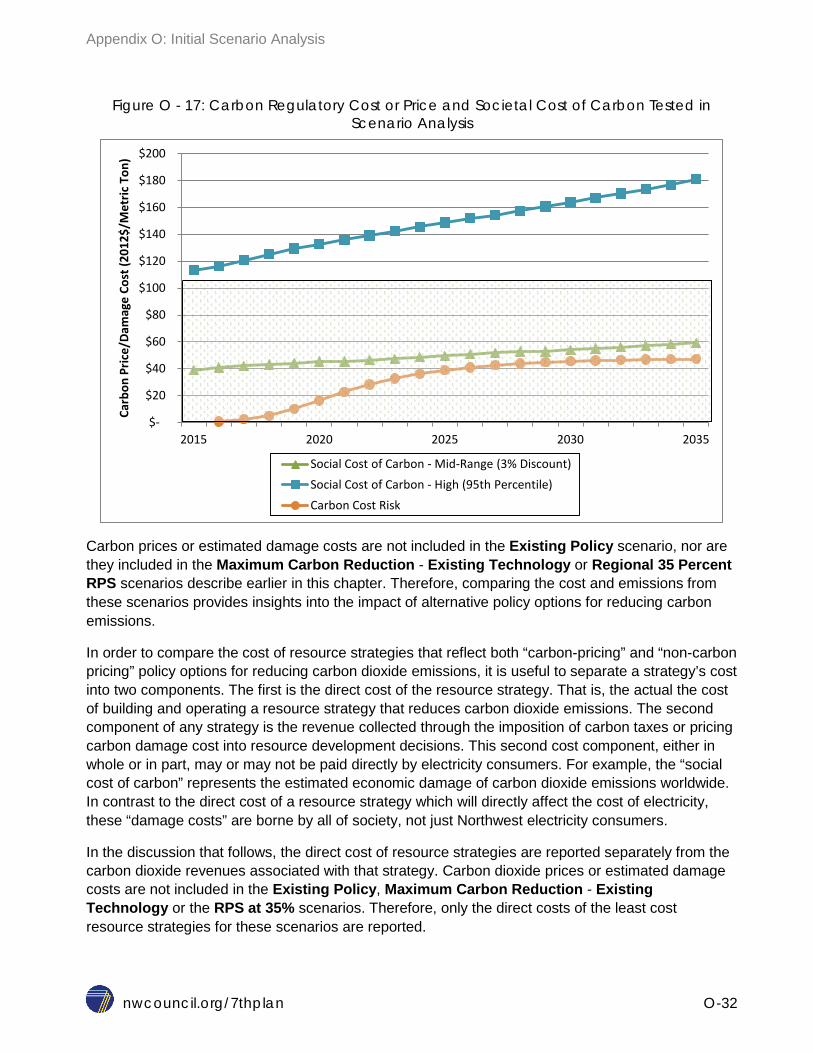
Appendix O: Initial Scenario Analysis
nwcouncil.org/7thplan O-32
Figure O - 17: Carbon Regulatory Cost or Price and Societal Cost of Carbon Tested in Scenario Analysis
Carbon prices or estimated damage costs are not included in the Existing Policy scenario, nor are they included in the Maximum Carbon Reduction - Existing Technology or Regional 35 Percent RPS scenarios describe earlier in this chapter. Therefore, comparing the cost and emissions from these scenarios provides insights into the impact of alternative policy options for reducing carbon emissions.
In order to compare the cost of resource strategies that reflect both “carbon-pricing” and “non-carbon pricing” policy options for reducing carbon dioxide emissions, it is useful to separate a strategy’s cost into two components. The first is the direct cost of the resource strategy. That is, the actual the cost of building and operating a resource strategy that reduces carbon dioxide emissions. The second component of any strategy is the revenue collected through the imposition of carbon taxes or pricing carbon damage cost into resource development decisions. This second cost component, either in whole or in part, may or may not be paid directly by electricity consumers. For example, the “social cost of carbon” represents the estimated economic damage of carbon dioxide emissions worldwide. In contrast to the direct cost of a resource strategy which will directly affect the cost of electricity, these “damage costs” are borne by all of society, not just Northwest electricity consumers.
In the discussion that follows, the direct cost of resource strategies are reported separately from the carbon dioxide revenues associated with that strategy. Carbon dioxide prices or estimated damage costs are not included in the Existing Policy, Maximum Carbon Reduction - Existing Technology or the RPS at 35% scenarios. Therefore, only the direct costs of the least cost resource strategies for these scenarios are reported.
$-
$20
$40
$60
$80
$100
$120
$140
$160
$180
$200
2015 2020 2025 2030 2035
Carb
on P
rice/
Dam
age
Cost
(201
2$/M
etric
Ton
)
Social Cost of Carbon - Mid-Range (3% Discount) Social Cost of Carbon - High (95th Percentile) Carbon Cost Risk

Appendix O: Initial Scenario Analysis
nwcouncil.org/7thplan O-33
Figure O - 18 shows the direct resource strategy average system costs and carbon emissions from the ten scenarios and sensitivity studies conducted to specifically evaluate carbon emissions reduction policies (and risks) for the development of the Seventh Power Plan. This figure shows the average net present value system cost (bars) for the least cost resource strategy for each scenario, both with and without carbon tax revenues. It also shows the average carbon emissions projected for the generation that serves the region in 2035.
Figure O - 18: Average System Costs and PNW Power System Carbon Emissions by Scenario in 2035
Figure O - 18 shows the Existing Policy scenario results in carbon emissions in 2035 of 34 million metric tons. This scenario assumed no additional policies to reduce carbon emissions beyond currently announced coal plant retirements are pursued. The average present value system cost of this resource strategy is $88 billion (2012$). The Social Cost of Carbon – Mid-Range (SCC-Mid-Range) and Social Cost of Carbon – High-Range (SCC-High) scenarios reduce carbon emissions to about between 18 to 20 million metric tons in 2035. The average system cost, excluding the carbon tax revenues for these scenarios is $0.8 billion for the SCC – Mid-Range and $1.6 billion for the SCC – High more than the average system cost of the Existing Policy scenario.
Under the Carbon Cost Risk scenario, 2035 carbon emissions were reduced to 24 million metric tons, or 10 million metric tons below the Existing Policy scenario. The average present value cost of this scenario, net of carbon tax revenues is $0.7 billion above the Existing Policy scenario. Under the Maximum Carbon Reduction – Existing Technology scenario, 2035 carbon emissions are reduced to 12 million metric tons and average system cost is are approximately $20 billion over
- 5 10 15 20 25 30 35 40
$-
$20
$40
$60
$80
$100
$120
$140
2035
Car
bon
Emis
sion
s (M
MTE
/yr)
Net
Pre
sent
Val
ue S
yste
m C
ost
(bill
ion
2012
$)
Direct Cost of Resource Strategy
Direct Cost of Resource Strategy, plus CO2 Tax Revenues
CO2 Emissions in 2035 (MMTE)

Appendix O: Initial Scenario Analysis
nwcouncil.org/7thplan O-34
the Existing Policy scenario. The large increase in average system cost for this scenario over the Existing Policy case results from the replacement of all of the region’s existing coal and inefficient natural gas fleet with new, more efficient natural gas-fired combustion turbines.
The RPS at 35% scenario reduces 2035 carbon emissions to just under 30 million metric tons. This is a reduction of around 5 million metric tons per year compared to the Existing Policy scenario. The direct cost of this resource strategy is approximately $121 billion or $34 billion more than the Existing Policy scenario.
Comparing the results of these scenarios based on a single year’s emissions can be misleading. Each of these policies alters the resource selection and regional power system operation over the course of the entire study period. Figure O - 19 shows the annual emissions level for each scenario. A review of Figure O - 19 reveals that the two social cost of carbon scenarios, which assume carbon dioxide damage costs are imposed in 2016, immediately reduce carbon dioxide emissions and therefore have impacts throughout the entire twenty year period covered by the Seventh Plan. In contrast, the other three carbon dioxide reduction policies phase in over time, so there cumulative impacts are generally smaller.
Figure O - 19: Average Annual Carbon Emissions by Carbon Reduction Policy Scenario
The Carbon Cost Risk and RPS at 35% scenarios gradually reduce emissions, while the Maximum Carbon Reduction scenario dramatically reduces emission as existing coal and inefficient gas plants are retired post-2025. The difference in timing results in large differences in the cumulative carbon emissions reductions for these policies. All scenarios show gradually increasing emissions beginning around 2028 as the amount of annual conservation development slows due to the completion of cost-effective and achievable retrofits. This lower level of conservation no longer offsets regional load growth, leading to the increased use of CO2 emitting generation.
-
10
20
30
40
50
2015 2020 2025 2030 2035
Aver
age
Annu
al E
mis
sion
s (M
MTE
)
Existing Policy SCC - Mid-Range
SCC - High Carbon Cost Risk
Maximum Carbon Reduction - Existing Technology RPS at 35%

Appendix O: Initial Scenario Analysis
nwcouncil.org/7thplan O-35
Figure O - 20 shows the cumulative reduction in carbon emissions for the carbon reduction policy scenarios compared to the Existing Policy scenario.
Figure O - 20: Cumulative 2016 to 2035 Carbon Emissions Reductions for Carbon Policy Scenarios
A comparison of Figure O - 19 and Figure O - 20 shows that the largest cumulative emissions reductions do not necessarily result from policy options that produce the lowest emission rate in 2035. For example, both social cost of carbon scenarios result in higher emission levels in 2035 than the Maximum Carbon Reduction – Existing Technology scenario. However, both social cost of carbon scenarios also produce much larger cumulative reductions over the entire planning period.
It should be noted, that the differences in cumulative emissions across these policy options are largely an artifact of the scenario modeling assumptions, which assume immediate imposition of the social cost of carbon. It is unlikely that such large carbon damage cost would or could be imposed in a single step without serious economic disruption. Therefore, the cumulative carbon emission reductions from the implementation of a carbon pricing policy which phases in carbon cost over time, similar to the Carbon Cost Risk scenario, are likely more representative of the actual impacts of imposing a carbon price based on the social cost of carbon.
Table O - 4 shows cumulative emissions reduction in carbon from the Existing Policy for the five carbon reduction policy options and the incremental system cost net of carbon tax revenues. Table O - 4 reveals that three carbon pricing policies have roughly comparable cost per unit of carbon dioxide emission reduction, ranging from $2 to $4 per metric ton. The Maximum Carbon Reduction – Existing Technology scenario, as can be seen from Figure O - 19, results in the lowest average
0
50
100
150
200
250
300
350
400
450
500
RPS at 35% Carbon Cost Risk Maximum CO2 Reduction -
Existing Technology
SCC - Mid-Range SCC - High
Cum
ulat
ive
Emis
sion
s Re
duct
ion
(MM
TE)

Appendix O: Initial Scenario Analysis
nwcouncil.org/7thplan O-36
annual carbon emissions from the regional power system by 2035, but also has a significantly higher average system cost and cost per unit of carbon dioxide reduction ($90/metric ton).
It should be noted that the direct cost of the resource strategies shown for the three carbon-pricing policies are likely understated. This is because all of three scenarios, but especially the two social cost of carbon scenarios, result in immediate and significant reductions in the dispatch of the region’s existing coal-fired generation in the model. In practice, at such reduced levels of dispatch, most or all of these plants would likely be retired as uneconomic. As a result, the actual direct cost of carbon reduction under these scenarios would probably be closer to the Maximum Carbon Reduction – Existing Technology scenario.
Table O - 4: Average Cumulative Emissions Reductions and Present Value Cost of Alternative Carbon Emissions Reduction Policies Compared to Existing Policy Scenario
CO2 Emissions - PNW System 2016 - 2035 (MMTE)
Cumulative Emission Reduction
Over Existing Policy
Scenario (MMTE)
Incremental Average System
Cost Net of Carbon Tax Revenues Over Existing
Policy Scenario (billion 2012$)
Present Value Average
Cost/Metric of Carbon
Emissions Reduction
(2012$/Metric Ton)
SCC - Mid-Range
360 $ 0.8 $ 2
SCC - High
438 $ 1.5 $ 4
Carbon Cost Risk
196 $ 0.7 $ 3 Maximum Carbon Reduction - Existing Technology
217 $ 19.6 $ 90
RPS at 35%
87 $ 33.9 $ 389
In the analysis shown above, only the cost incurred during the planning period (i.e. 2016-2035) and the emissions reductions that occur during this same time frame are considered. Clearly, investments made to reduce carbon emissions will continue beyond 2035, as will their carbon emissions impacts. These “end-effects” could alter the perceived relative cost-efficiency of carbon reduction policy options. For example, over a longer period of time, the cumulative emissions reductions from the Maximum Carbon Reduction – Existing Technology scenario could exceed those from the Social Cost of Carbon – Mid-Range scenario because by 2035 the Maximum Carbon Reduction – Existing Technology scenario results in 8 MMTE per year lower emissions. In this instance, if the difference in emission rates for these two scenarios were to remain the same for an additional 20 years, then their cumulative emissions reductions over 40 years would be nearly identical. Considering these “end effects”, care should be exercised inferring the most effective method for reducing carbon emissions. The cumulative emissions reductions shown in Table O - 4 can be misleading if not considered with the context of these effects.

Appendix O: Initial Scenario Analysis
nwcouncil.org/7thplan O-37
Maximum Carbon Reduction – Emerging Technology
In the preceding discussion the lower bound on regional power system carbon dioxide emissions was limited by existing technology. Under that constraint, the annual carbon dioxide emissions from the regional power system could be reduced from an average of 55 million metric tons per year today to approximately 12 million metric tons in 2035.8 While this represents nearly an 80 percent reduction in emissions, it does not eliminate power system carbon dioxide emissions entirely. In order to achieve that policy goal, new and emerging technology must be developed and deployed.
To assess the magnitude of potential additional carbon dioxide emission reductions that might be feasible by 2035, the Council created a resource strategy based on energy efficiency resources and non-carbon dioxide emitting generating resource alternatives that might become commercially viable over the next 20 years. While the Regional Portfolio Model (RPM) was used to develop the amount, timing and mix of resources in this resource strategy, no economic constraints were taken into account. That is, the RPM was simply used create a mix of resources that could meet forecast energy and capacity needs, but it made no attempt to minimize the cost to do so. The reason the RPM’s economic optimization logic was not used is that the future cost and resource characteristics of many of the emerging technologies included in this scenario are highly speculative.
Tables O - 5 and O - 6 summarize the potential resource size and cost of energy efficiency and generating resource emerging technologies considered in this scenario that were modeled in the RPM. A review of Table O - 5 shows that an additional 650 average megawatts of emerging energy efficiency technology could be deployed by 2025. If this technology were cost-effective to acquire, it could reduce winter peak demands in that year by 1,350 megawatts. Five years later, by 2030, potential annual energy savings could reach 1,125 average megawatts and reduce winter peak demands by 2,350 megawatts. Only about one-third of these potential savings is currently forecast to cost less than $30 per megawatt-hour and the remaining two-thirds of the potential savings is anticipated to cost more than $80 per megawatt-hour. See Chapter 12 and Appendix G for a more detailed discussion of these emerging energy efficiency technologies.
The regional potential of both utility scale and especially distributed solar PV resources, as shown in Table O - 6, is quite large. Assuming significant cost reductions in utility scale solar PV system installations by 2030, the levelized cost of power produced from such systems could be around $50 per megawatt-hour. However, while both utility scale and distributed solar PV systems can significantly contribute to meeting summer peak requirements, they provide little or no winter peak savings. In the near term, this limits their applicability to the region’s needs. However, since the region’s summer peak demands are forecast to grow more rapidly than winter peak demands, the system peak benefits of these systems are expected to increase over time. See Chapter 11 and Appendix H for a more detailed discussion of these emerging technologies.
Figure O - 21 shows the distribution of annual carbon dioxide emissions in 2035 for both the Maximum Carbon Reduction – Existing Technology and Maximum Carbon Reduction – Emerging Technology scenarios. Inspection of Figure O - 21 reveals that with existing technology
8 Average regional power system carbon dioxide emissions from 2000 – 2012 were approximately 55 million metric tons.

Appendix O: Initial Scenario Analysis
nwcouncil.org/7thplan O-38
carbon dioxide emissions can be reduced to 12 million metric tons per year by 2035. If the emerging energy efficiency and renewable resource technologies shown in Tables O - 5 and O - 6 are available for deployment, carbon dioxide emissions in 2035 could be reduced to 6 million metric tons per year. The range in annual carbon dioxide emissions for both scenarios is largely driven by Northwest hydroelectric generation output and future load growth. However, under the scenario where emerging technology becomes available, the range of future emissions is narrower, largely due to less reliance on natural gas-fired generation under low water conditions.

Chapter 15: Analysis of Alternative Resource Strategies
nwcouncil.org/7thplan 15-39
Table O - 5: Energy Efficiency Emerging Technologies Modeled in the RPM in the Maximum Carbon Reduction – Emerging Technology Scenario
Emerging Technology
Regional Potential - 2025 Regional Potential - 2030
Energy (aMW)
Winter Peak
Capacity (MW)
TRC Net Levelized
Cost (2012$ /MWh)
Energy (aMW)
Winter Peak
Capacity (MW)
TRC Net Levelized
Cost (2012$ /MWh)
Additional Advances in Solid-State Lighting 200 400 $0-$30 400 800 $0-$30 CO2 Heat Pump Water Heater 110 200 $100-150 160 300 $90-140
CO2 Heat Pump Space Heating 50 160 $130-170 130 350 $110-160 Highly Insulated Dynamic Windows - Commercial 20 130 $500+ 35 200 300 Highly Insulated Dynamic Windows - Residential 80 230 $500+ 120 350 400 HVAC Controls – Optimized Controls 140 230 $90-120 200 350 $80-110 Evaporative Cooling 50 0* $100-130 80 0* $90-120 Total 650 1,350 N/A 1,125 2,350 N/A
Table O - 6: Non-Carbon Dioxide Emitting Generating Emerging Technologies Modeled in the RPM in the Maximum Carbon Reduction – Emerging Technology Scenario
Utility Scale 48 MW Solar PV Plant – Southern Idaho
Utility Scale 48 MW Solar PV Plant – Kelso WA
Distributed Solar (Residential and Commercial Sectors)
Potential regional installed capacity = 528 MW
Potential regional installed capacity = 1,440 MW
Potential regional installed capacity = 28,100 MW
Year Energy (aMW)
Winter Peak (MW)
Summer Peak (MW)
Real Levelized
Cost (2012$ /MWh)
Energy (aMW)
Winter Peak (MW)
Summer Peak (MW)
Real Levelized
Cost (2012$ /MWh)
Energy (aMW)
Winter Peak (MW)
Summer Peak (MW)
Real Levelized
Cost (2012$ /MWh)*
2020 12 - 24 $66 9 - 24 $89 340 2 700 $180 2025 12 - 24 $58 9 - 24 $77 1350 6 2800 $170 2030 12 - 24 $51 9 - 24 $68 2880 13 6000 $150 2035 12 - 24 $51 9 - 24 $67 4000 18 8300 $150 *High penetration of distributed solar resources will likely require additional integration cost and distribution system upgrades

Seventh Northwest Conservation and Electric Power Plan
nwcouncil.org/7thplan 15-40
Figure O - 21: Distribution of Annual Carbon Dioxide Emissions Under Maximum Carbon Reduction Scenarios With and Without Emerging Technology
The difference in annual resource dispatch over time between the Maximum Carbon Reduction – Emerging Technology scenario and the Maximum Carbon Reduction – Existing Technology scenario is shown in Figure O - 22. As can be observed from Figure O - 22 the primary differences is the increased amount of energy efficiency and renewable resources developed (shown by the bars above the origin on the vertical axis) under the emerging technology scenario and less reliance on both existing and new gas-fired generation (shown by the wedges below the origin on the vertical axis). It should be emphasized that under the emerging technology scenario this tradeoff between new natural gas generation and emerging conservation and renewable resource development is not based on economics. Rather, their development occurs because new natural gas-fired generation was specifically excluded from consideration under the emerging technology scenario.
Figure O - 22 shows that under the Maximum Carbon Reduction – Emerging Technology scenario just over 2,000 average megawatts of gas-fired generation must be displaced by approximately 2,500 average megawatts of renewable resources and 1,750 average megawatts of additional energy efficiency. The large difference in the amount of natural gas resources displaced versus the amount of conservation and renewable resources added reflects the limited contribution to supplying winter peak demands provided by solar PV and wind resources.
In order to lower the cost of achieving the carbon emissions reductions in the Maximum Carbon Reduction - Emerging Technology scenario and/or to further reduce the power system’s carbon
0%
2%
4%
6%
8%
10%
12%
14%
16%
18%
20%
0 2 4 6 8 10 12 14 16 18 20 22 24 26 28 30 32 34 36 38
Prob
abili
ty o
f Occ
uran
ce
Annual Carbon Dioxide Emissions in 2035 (MMTE)
Maximum Carbon Reduction - Existing Technology
Maximum Carbon Reduction - EmergingTechnology
Average Emission with Emerging Technology = 6 MMTE
Average Emissions with Existing Technology = 12 MMTE
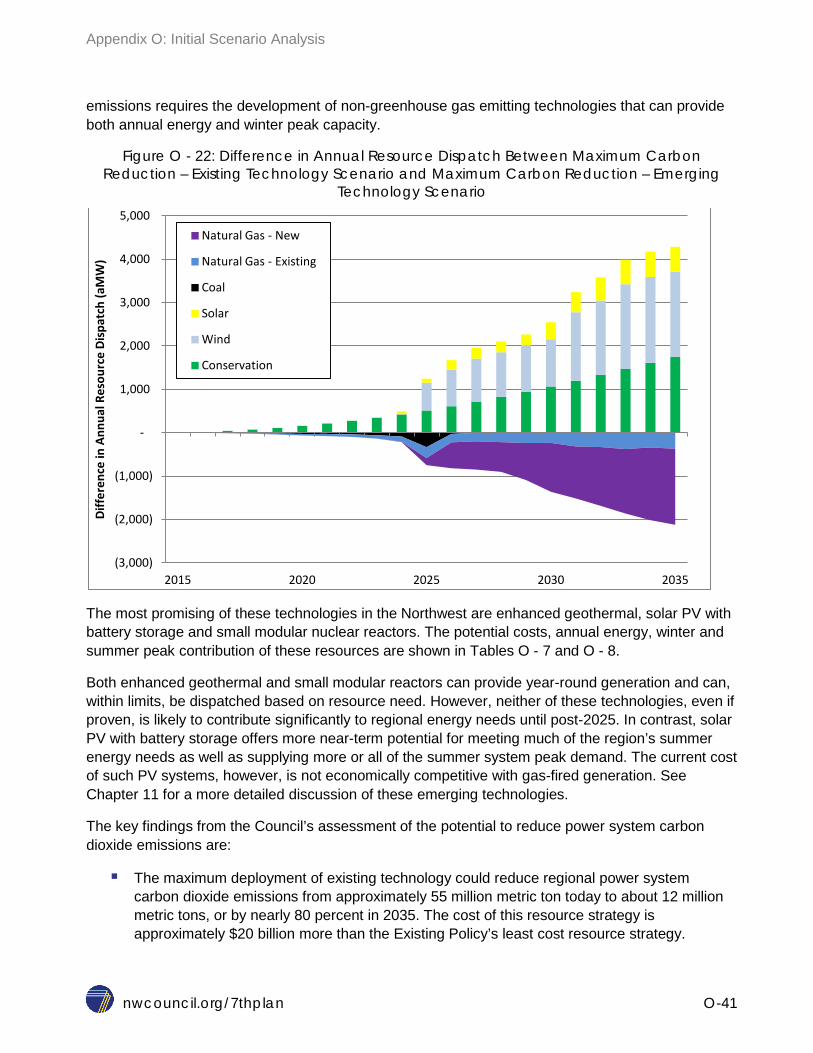
Appendix O: Initial Scenario Analysis
nwcouncil.org/7thplan O-41
emissions requires the development of non-greenhouse gas emitting technologies that can provide both annual energy and winter peak capacity.
Figure O - 22: Difference in Annual Resource Dispatch Between Maximum Carbon Reduction – Existing Technology Scenario and Maximum Carbon Reduction – Emerging
Technology Scenario
The most promising of these technologies in the Northwest are enhanced geothermal, solar PV with battery storage and small modular nuclear reactors. The potential costs, annual energy, winter and summer peak contribution of these resources are shown in Tables O - 7 and O - 8.
Both enhanced geothermal and small modular reactors can provide year-round generation and can, within limits, be dispatched based on resource need. However, neither of these technologies, even if proven, is likely to contribute significantly to regional energy needs until post-2025. In contrast, solar PV with battery storage offers more near-term potential for meeting much of the region’s summer energy needs as well as supplying more or all of the summer system peak demand. The current cost of such PV systems, however, is not economically competitive with gas-fired generation. See Chapter 11 for a more detailed discussion of these emerging technologies.
The key findings from the Council’s assessment of the potential to reduce power system carbon dioxide emissions are:
The maximum deployment of existing technology could reduce regional power system carbon dioxide emissions from approximately 55 million metric ton today to about 12 million metric tons, or by nearly 80 percent in 2035. The cost of this resource strategy is approximately $20 billion more than the Existing Policy’s least cost resource strategy.
(3,000)
(2,000)
(1,000)
-
1,000
2,000
3,000
4,000
5,000
2015 2020 2025 2030 2035
Diffe
renc
e in
Ann
ual R
esou
rce
Disp
atch
(aM
W)
Natural Gas - New
Natural Gas - Existing
Coal
Solar
Wind
Conservation

Appendix O: Initial Scenario Analysis
nwcouncil.org/7thplan O-42
With development and deployment of emerging energy efficiency and non-carbon emitting resource technologies, it may be possible to reduce 2035 regional power system carbon dioxide emissions to approximately 6 million metric tons, or to about 50 percent below the level achievable with existing technology by 2035.
At present, it is not possible to entirely eliminate carbon dioxide emissions from the power system without the development and deployment of emerging technology for both energy efficiency and non-carbon dioxide emitting generation that require technological or cost breakthroughs.
Deployment of variable output renewable resources at the scale considered in the Maximum Carbon Reduction – Emerging Technology scenario will presents significant power system operational challenges.
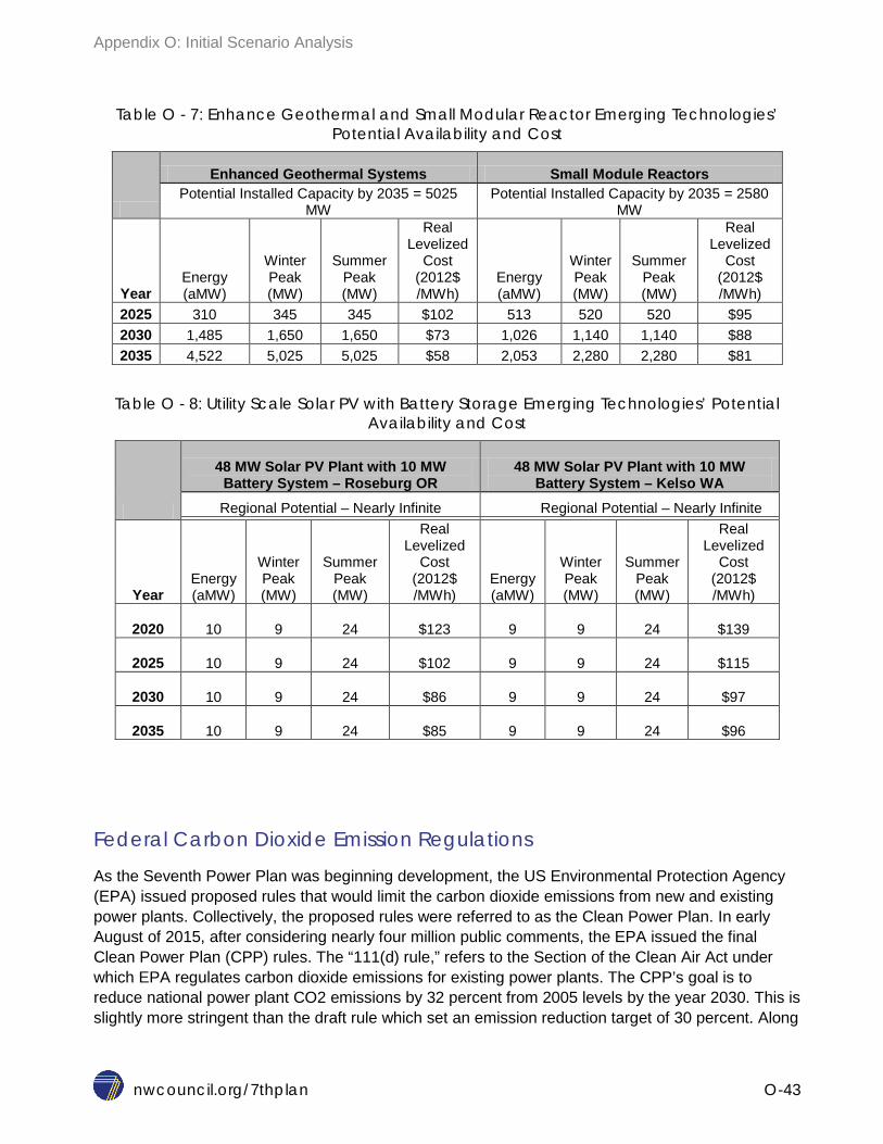
Appendix O: Initial Scenario Analysis
nwcouncil.org/7thplan O-43
Table O - 7: Enhance Geothermal and Small Modular Reactor Emerging Technologies’ Potential Availability and Cost
Enhanced Geothermal Systems Small Module Reactors Potential Installed Capacity by 2035 = 5025
MW Potential Installed Capacity by 2035 = 2580
MW
Year Energy (aMW)
Winter Peak (MW)
Summer Peak (MW)
Real Levelized
Cost (2012$ /MWh)
Energy (aMW)
Winter Peak (MW)
Summer Peak (MW)
Real Levelized
Cost (2012$ /MWh)
2025 310 345 345 $102 513 520 520 $95 2030 1,485 1,650 1,650 $73 1,026 1,140 1,140 $88 2035 4,522 5,025 5,025 $58 2,053 2,280 2,280 $81
Table O - 8: Utility Scale Solar PV with Battery Storage Emerging Technologies’ Potential Availability and Cost
48 MW Solar PV Plant with 10 MW Battery System – Roseburg OR
48 MW Solar PV Plant with 10 MW Battery System – Kelso WA
Regional Potential – Nearly Infinite Regional Potential – Nearly Infinite
Year Energy (aMW)
Winter Peak (MW)
Summer Peak (MW)
Real Levelized
Cost (2012$ /MWh)
Energy (aMW)
Winter Peak (MW)
Summer Peak (MW)
Real Levelized
Cost (2012$ /MWh)
2020
10 9
24 $123
9
9
24 $139
2025
10 9
24 $102
9
9
24 $115
2030
10 9
24 $86
9
9
24 $97
2035
10 9
24 $85
9
9
24 $96
Federal Carbon Dioxide Emission Regulations
As the Seventh Power Plan was beginning development, the US Environmental Protection Agency (EPA) issued proposed rules that would limit the carbon dioxide emissions from new and existing power plants. Collectively, the proposed rules were referred to as the Clean Power Plan. In early August of 2015, after considering nearly four million public comments, the EPA issued the final Clean Power Plan (CPP) rules. The “111(d) rule,” refers to the Section of the Clean Air Act under which EPA regulates carbon dioxide emissions for existing power plants. The CPP’s goal is to reduce national power plant CO2 emissions by 32 percent from 2005 levels by the year 2030. This is slightly more stringent than the draft rule which set an emission reduction target of 30 percent. Along

Appendix O: Initial Scenario Analysis
nwcouncil.org/7thplan O-44
with the 111(d) rule, the EPA also issued the final rule under the Clean Air Act section 111(b) for new, as opposed to existing, power plants and the EPA also proposed a federal plan and model rules that would combine the two emissions limits.
To ensure the 2030 emissions goals are met, the CPP requires states begin reducing their emissions no later than 2022 which is the start of an eight year compliance period. During the compliance period, states need to achieve progressively increasing reductions in CO2 emissions. The eight year interim compliance period is further broken down into three periods, 2022-2024, 2025-2027, and 2028-2029, each associated with its own interim emission reduction goals.
Under the EPA’s final rules, states may comply by reducing the average carbon emission rate (pounds of CO2 per kilowatt-hour) of all power generating facilities located within their state that are covered by the rule. In the alternative, states may comply by limiting the total emissions (tons of CO2 per year) from those plants. The former compliance option is referred as a “rate-based” path, while the latter compliance option is referred to as a “mass-based” path. Under the “mass-based” compliance option, EPA has set forth two alternative limits on total CO2 emissions. The first, and lower limit, includes only emissions from generating facilities either operating or under constructions as of January 8, 2014. The second, and higher limit, includes emissions from both existing and new generating facilities, effectively combining the 111(b) and 111(d) regulations.
The Council determined that a comparison of the carbon emissions from alternative resource strategies should be based on the emissions from both existing and new facilities covered by the EPA’s regulations. This approach is a better representation of the total carbon footprint of the region’s power system and is more fully able to capture the benefits of using energy efficiency as an option for compliance because it reduces the need for new generation. Table O - 9 shows the final rule’s emission limits for the four Northwest states for the “mass-based” compliance path, including both existing and new generation.
Table O - 9: Pacific Northwest States’ Clean Power Plan Final Rule CO2 Emissions Limits9
Mass Based Goal (Existing) and New Source Complement (Million Metric Tons) Period Idaho Montana Oregon Washington PNW
Interim Period 2022-29
1.49
11.99
8.25
11.08
32.8
2022 to 2024
1.51
12.68
8.45
11.48
34.1
2025 to 2027
1.48
11.80
8.18
10.95
32.4
2028 to 2029
1.48
11.23
8.06
10.67
31.4
2030 and Beyond
1.49
10.85
8.00
10.49
30.8
9 Note: EPA’s emissions limits are stated in the regulation in “short tons” (2000 lbs). In Table O - 9 and throughout this document, carbon dioxide emissions are measured in “metric tons” (2204.6 lbs) or million metric ton equivalent (MMTE).
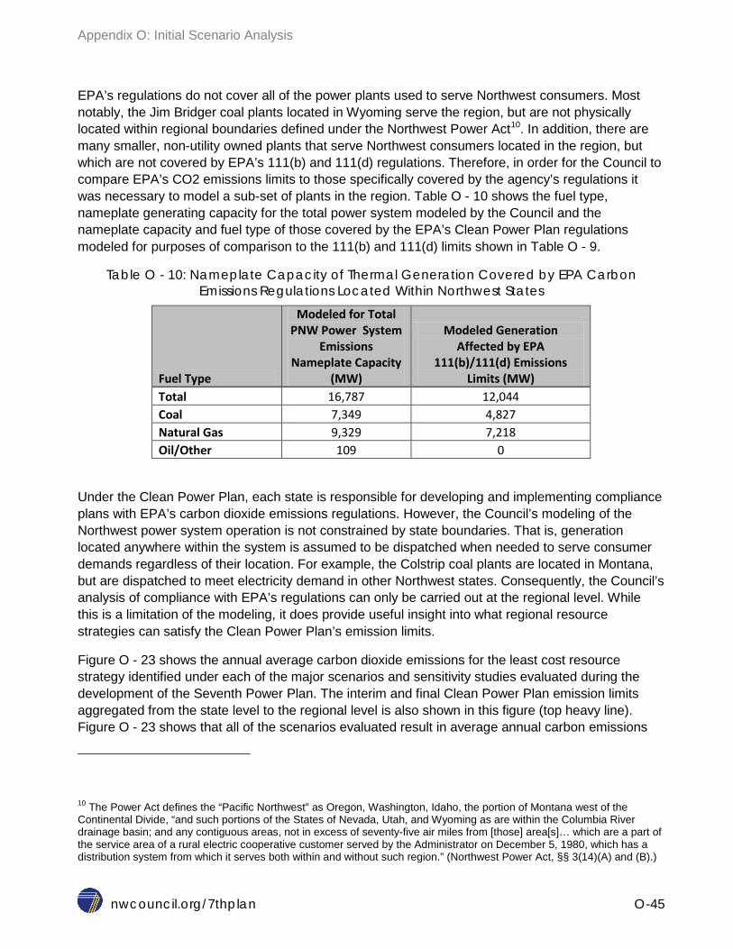
Appendix O: Initial Scenario Analysis
nwcouncil.org/7thplan O-45
EPA’s regulations do not cover all of the power plants used to serve Northwest consumers. Most notably, the Jim Bridger coal plants located in Wyoming serve the region, but are not physically located within regional boundaries defined under the Northwest Power Act10. In addition, there are many smaller, non-utility owned plants that serve Northwest consumers located in the region, but which are not covered by EPA’s 111(b) and 111(d) regulations. Therefore, in order for the Council to compare EPA’s CO2 emissions limits to those specifically covered by the agency’s regulations it was necessary to model a sub-set of plants in the region. Table O - 10 shows the fuel type, nameplate generating capacity for the total power system modeled by the Council and the nameplate capacity and fuel type of those covered by the EPA’s Clean Power Plan regulations modeled for purposes of comparison to the 111(b) and 111(d) limits shown in Table O - 9.
Table O - 10: Nameplate Capacity of Thermal Generation Covered by EPA Carbon Emissions Regulations Located Within Northwest States
Fuel Type
Modeled for Total PNW Power System
Emissions Nameplate Capacity
(MW)
Modeled Generation Affected by EPA
111(b)/111(d) Emissions Limits (MW)
Total 16,787 12,044 Coal 7,349 4,827 Natural Gas 9,329 7,218 Oil/Other 109 0
Under the Clean Power Plan, each state is responsible for developing and implementing compliance plans with EPA’s carbon dioxide emissions regulations. However, the Council’s modeling of the Northwest power system operation is not constrained by state boundaries. That is, generation located anywhere within the system is assumed to be dispatched when needed to serve consumer demands regardless of their location. For example, the Colstrip coal plants are located in Montana, but are dispatched to meet electricity demand in other Northwest states. Consequently, the Council’s analysis of compliance with EPA’s regulations can only be carried out at the regional level. While this is a limitation of the modeling, it does provide useful insight into what regional resource strategies can satisfy the Clean Power Plan’s emission limits.
Figure O - 23 shows the annual average carbon dioxide emissions for the least cost resource strategy identified under each of the major scenarios and sensitivity studies evaluated during the development of the Seventh Power Plan. The interim and final Clean Power Plan emission limits aggregated from the state level to the regional level is also shown in this figure (top heavy line). Figure O - 23 shows that all of the scenarios evaluated result in average annual carbon emissions
10 The Power Act defines the “Pacific Northwest” as Oregon, Washington, Idaho, the portion of Montana west of the Continental Divide, “and such portions of the States of Nevada, Utah, and Wyoming as are within the Columbia River drainage basin; and any contiguous areas, not in excess of seventy-five air miles from [those] area[s]… which are a part of the service area of a rural electric cooperative customer served by the Administrator on December 5, 1980, which has a distribution system from which it serves both within and without such region.” (Northwest Power Act, §§ 3(14)(A) and (B).)

Appendix O: Initial Scenario Analysis
nwcouncil.org/7thplan O-46
well below the EPA limits for the region. This includes two of the scenarios that were specifically designed to “stress test” whether the region would be able to comply with s the Clean Power Plan’s emission limits if one or more existing non-carbon emitting resources in the region were taken out of service.
In the Unplanned Loss of a Major Resource scenario, it was assumed that a single large resource that does not emit carbon dioxide with 1,200 megawatts of nameplate capacity, producing 1,000 average megawatts of energy would randomly and permanently discontinue operation sometime over the next 20 years. Because this scenario was designed to test the vulnerability of the region’s ability to comply with the Clean Power Plan’s emission limits in 2030, it was assumed that there was a 75 percent probability that this resource would discontinue operation by 2030 and a 100 percent probability it would do so by 2035. In the second scenario, the Planned Loss of a Major Resource, it was assumed that a total of 1,000 megawatts nameplate capacity producing 855 average megawatts of energy resources that do not emit carbon dioxide were retired by 2030. A review of Figure O - 23 shows that under both scenarios the average regional carbon dioxide emissions are well below the EPA’s limits for 2030 and beyond. One of the key findings from the Council’s analysis is that from a regional perspective compliance with EPA’s carbon emissions rule should be achievable without adoption of additional carbon reduction policies in the region. This is not to say that no additional action is required.
All of the least cost resource strategies that have their emission levels depicted in Figure O - 23 call for the development of between 4,000 and 4,600 average megawatts of energy efficiency by 2035. All of these resource strategies also assume that the retiring Centralia, Boardman and North Valmy coal plants are replaced with only those resources required to meet regional capacity and energy adequacy requirements. Utility development of new gas-fired generation to meet local needs for ancillary services, such as wind integration, or capacity requirements beyond the modest levels included under these scenarios are not modeled and would increase regional emissions. All of the least cost resource strategies also assume that Northwest electricity generation is dispatched to meet regional adequacy standards for energy and capacity rather than to serve external markets.

Appendix O: Initial Scenario Analysis
nwcouncil.org/7thplan O-47
Figure O - 23: Average Annual Carbon Dioxide Emissions for Least Cost Resource Strategies by Scenario for Generation Covered by the Clean Power Plan and Located Within
Northwest States
Resource Strategy Cost and Revenue Impacts The Council’s Regional Portfolio Model (RPM) calculates the net present value cost to the region of each resource strategy to identify the strategies that have both low cost and low risk. The RPM includes only the forward-going costs of the power system; that is, only those costs that can be affected by future conditions and resource decisions. Figure O - 24 shows the present value system cost for the principal scenarios evaluated during the development of the Seventh Power Plan. Figure O - 24 also shows the present value of power system costs both with and without assumed carbon tax revenues. That is, the scenarios that assumed some form of carbon price include not only the direct cost of building and operating the resource strategy, but also the revenues from carbon dioxide taxes assumed in those scenarios. Of course those scenarios without a carbon price, the Low Gas Price and Existing Policy scenarios have the same average system cost in both cases.
-
5
10
15
20
25
30
35
40
2015 2020 2025 2030 2035
Annu
al F
our-
Stat
e CO
2 Em
issi
ons
(M
MTE
)
Existing Policy, No Carbon Risk Social Cost of Carbon - Base Social Cost of Carbon - High Carbon Risk Maximum CO2 Reduction Unplanned Loss of Major Resource Planned Loss of Major Resource RPS at 35% EPA Emissions Limits
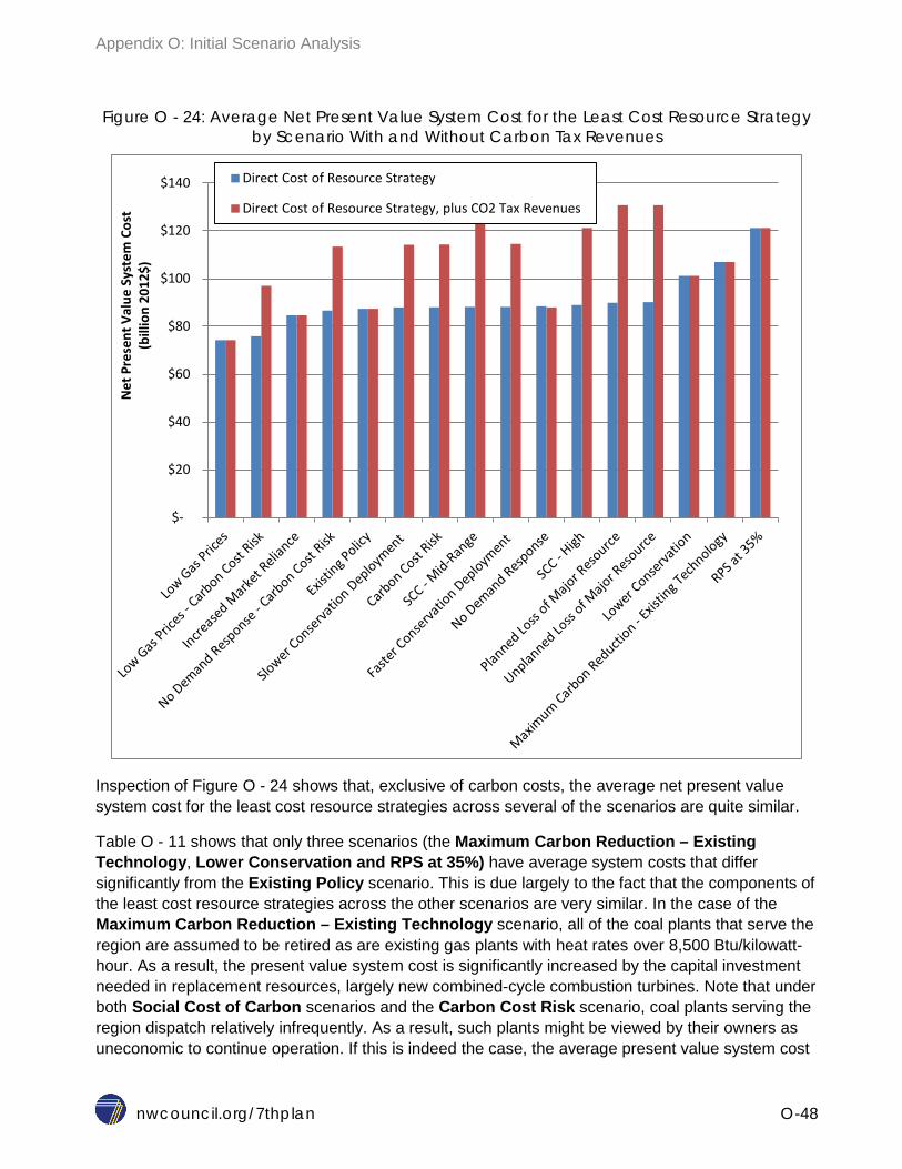
Appendix O: Initial Scenario Analysis
nwcouncil.org/7thplan O-48
Figure O - 24: Average Net Present Value System Cost for the Least Cost Resource Strategy by Scenario With and Without Carbon Tax Revenues
Inspection of Figure O - 24 shows that, exclusive of carbon costs, the average net present value system cost for the least cost resource strategies across several of the scenarios are quite similar.
Table O - 11 shows that only three scenarios (the Maximum Carbon Reduction – Existing Technology, Lower Conservation and RPS at 35%) have average system costs that differ significantly from the Existing Policy scenario. This is due largely to the fact that the components of the least cost resource strategies across the other scenarios are very similar. In the case of the Maximum Carbon Reduction – Existing Technology scenario, all of the coal plants that serve the region are assumed to be retired as are existing gas plants with heat rates over 8,500 Btu/kilowatt-hour. As a result, the present value system cost is significantly increased by the capital investment needed in replacement resources, largely new combined-cycle combustion turbines. Note that under both Social Cost of Carbon scenarios and the Carbon Cost Risk scenario, coal plants serving the region dispatch relatively infrequently. As a result, such plants might be viewed by their owners as uneconomic to continue operation. If this is indeed the case, the average present value system cost
$-
$20
$40
$60
$80
$100
$120
$140
Net
Pre
sent
Val
ue S
yste
m C
ost
(bill
ion
2012
$)
Direct Cost of Resource Strategy
Direct Cost of Resource Strategy, plus CO2 Tax Revenues

Appendix O: Initial Scenario Analysis
nwcouncil.org/7thplan O-49
of these scenarios would likely be much closer to the Maximum Carbon Reduction – Existing Technology scenario.
The least cost resource strategy under the Lower Conservation scenario develops about 1,200 average megawatts less energy savings and 2,900 megawatts less of winter peak capacity from energy efficiency by 2035 than the Existing Policy scenario. As a result, its average system cost is nearly $14 billion higher because it must substitute more expensive generating resources to meet the region’s needs for both capacity and energy.
Under the Regional 35 Percent RPS scenario, the increase in average present value system cost stems from the investment needed to develop a significant quantity of additional wind and solar generation in the region to satisfy the higher standard. The average present value system cost for the least cost resource strategy under the Increased Market Reliance scenario is lower because fewer resources are developed in the region to meet regional resource adequacy standards, resulting in lower future costs.
Table O - 11: Average Net Present Value System Cost with Carbon Cost and Incremental Cost Compared to Existing Policy, No Carbon Risk Scenario
Scenario
System Cost Without Carbon Tax Revenues
(billion 2012$)
Incremental Cost Over Existing Policy
Scenario (billion 2012$) Existing Policy $87 Social Cost of Carbon – Mid-Range $88 $0.8 Social Cost of Carbon – High-Range $89 $1.5 Carbon Risk $88 $0.7 Maximum CO2 Reduction – Existing Technology $107 $19.6 Unplanned Loss of Major Resource $90 $2.8 Planned Loss of Major Resource $90 $2.5 Faster Conservation Deployment $88 $0.8 Slower Conservation Deployment $88 $0.6 Increased Reliance on External Markets $85 ($2.7) Regional 35 Percent RPS $121 $33.9 Lower Conservation – No Carbon Risk $101 $13.8
Reporting costs as net present values does not show patterns over time and may obscure differences among individual utilities. The latter is unavoidable in regional planning and the Council has noted throughout the plan that different utilities will be affected differently by alternative policies. It is possible, however, to display the temporal patterns of costs among scenarios. Figure O - 25 shows forward-going power system costs for selected scenarios on an annual basis.
Forward-going costs include only the future operating costs of existing resources and the capital and operating costs of new resources. The 2016 value in Figure O - 25 includes mainly operating costs of the current power system, but not the capital costs of the existing generation, transmission, and distribution system since these remain unchanged by future resource decisions. The cost shown for
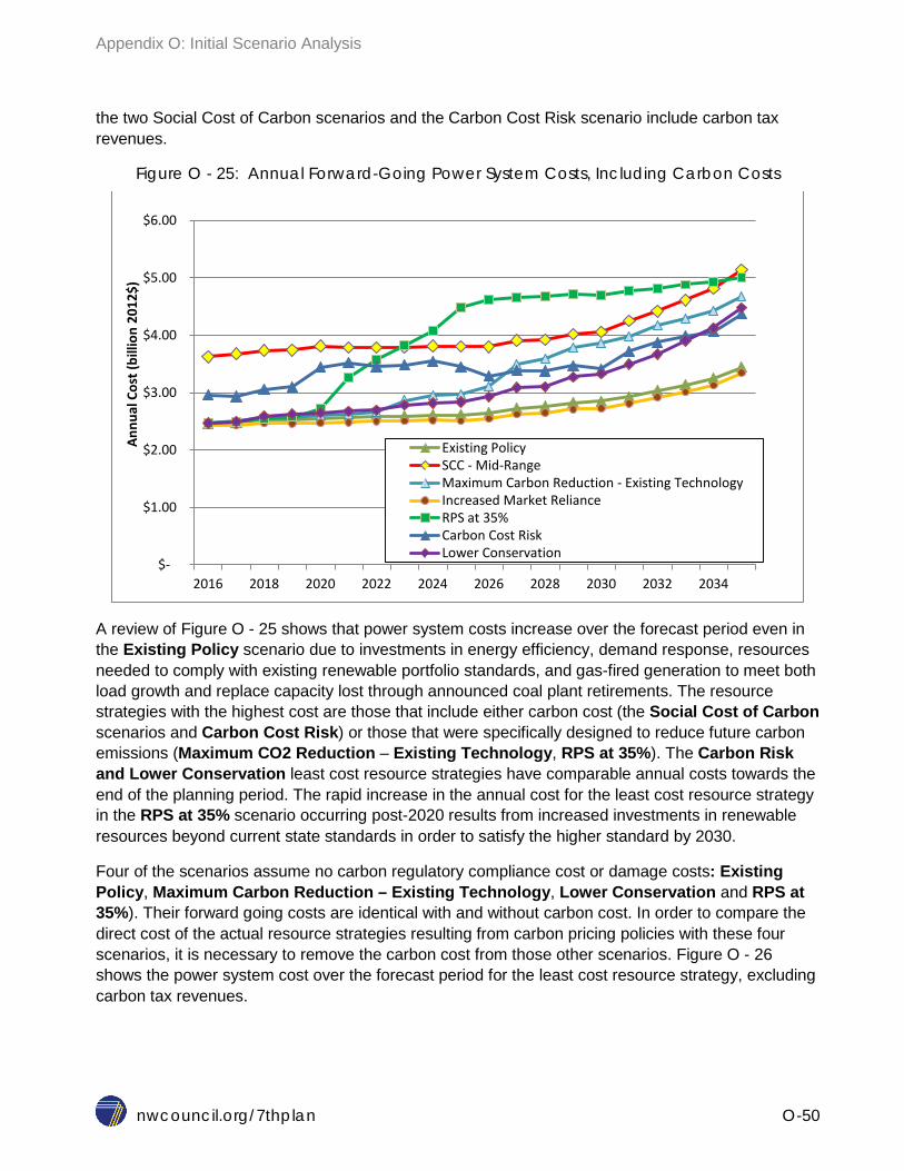
Appendix O: Initial Scenario Analysis
nwcouncil.org/7thplan O-50
the two Social Cost of Carbon scenarios and the Carbon Cost Risk scenario include carbon tax revenues.
Figure O - 25: Annual Forward-Going Power System Costs, Including Carbon Costs
A review of Figure O - 25 shows that power system costs increase over the forecast period even in the Existing Policy scenario due to investments in energy efficiency, demand response, resources needed to comply with existing renewable portfolio standards, and gas-fired generation to meet both load growth and replace capacity lost through announced coal plant retirements. The resource strategies with the highest cost are those that include either carbon cost (the Social Cost of Carbon scenarios and Carbon Cost Risk) or those that were specifically designed to reduce future carbon emissions (Maximum CO2 Reduction – Existing Technology, RPS at 35%). The Carbon Risk and Lower Conservation least cost resource strategies have comparable annual costs towards the end of the planning period. The rapid increase in the annual cost for the least cost resource strategy in the RPS at 35% scenario occurring post-2020 results from increased investments in renewable resources beyond current state standards in order to satisfy the higher standard by 2030.
Four of the scenarios assume no carbon regulatory compliance cost or damage costs: Existing Policy, Maximum Carbon Reduction – Existing Technology, Lower Conservation and RPS at 35%). Their forward going costs are identical with and without carbon cost. In order to compare the direct cost of the actual resource strategies resulting from carbon pricing policies with these four scenarios, it is necessary to remove the carbon cost from those other scenarios. Figure O - 26 shows the power system cost over the forecast period for the least cost resource strategy, excluding carbon tax revenues.
$-
$1.00
$2.00
$3.00
$4.00
$5.00
$6.00
2016 2018 2020 2022 2024 2026 2028 2030 2032 2034
Annu
al C
ost (
billi
on 2
012$
)
Existing Policy SCC - Mid-Range Maximum Carbon Reduction - Existing Technology Increased Market Reliance RPS at 35% Carbon Cost Risk Lower Conservation
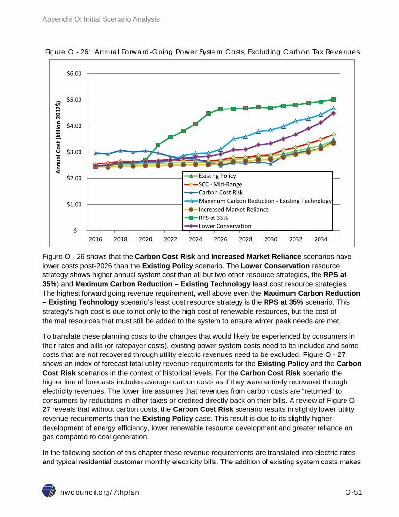
Appendix O: Initial Scenario Analysis
nwcouncil.org/7thplan O-51
Figure O - 26: Annual Forward-Going Power System Costs, Excluding Carbon Tax Revenues
Figure O - 26 shows that the Carbon Cost Risk and Increased Market Reliance scenarios have lower costs post-2026 than the Existing Policy scenario. The Lower Conservation resource strategy shows higher annual system cost than all but two other resource strategies, the RPS at 35%) and Maximum Carbon Reduction – Existing Technology least cost resource strategies. The highest forward going revenue requirement, well above even the Maximum Carbon Reduction – Existing Technology scenario’s least cost resource strategy is the RPS at 35% scenario. This strategy's high cost is due to not only to the high cost of renewable resources, but the cost of thermal resources that must still be added to the system to ensure winter peak needs are met.
To translate these planning costs to the changes that would likely be experienced by consumers in their rates and bills (or ratepayer costs), existing power system costs need to be included and some costs that are not recovered through utility electric revenues need to be excluded. Figure O - 27 shows an index of forecast total utility revenue requirements for the Existing Policy and the Carbon Cost Risk scenarios in the context of historical levels. For the Carbon Cost Risk scenario the higher line of forecasts includes average carbon costs as if they were entirely recovered through electricity revenues. The lower line assumes that revenues from carbon costs are “returned” to consumers by reductions in other taxes or credited directly back on their bills. A review of Figure O - 27 reveals that without carbon costs, the Carbon Cost Risk scenario results in slightly lower utility revenue requirements than the Existing Policy case. This result is due to its slightly higher development of energy efficiency, lower renewable resource development and greater reliance on gas compared to coal generation.
In the following section of this chapter these revenue requirements are translated into electric rates and typical residential customer monthly electricity bills. The addition of existing system costs makes
$-
$1.00
$2.00
$3.00
$4.00
$5.00
$6.00
2016 2018 2020 2022 2024 2026 2028 2030 2032 2034
Annu
al C
ost (
billi
on 2
012$
)
Existing Policy SCC - Mid-Range Carbon Cost Risk Maximum Carbon Reduction - Existing Technology Increased Market Reliance RPS at 35% Lower Conservation
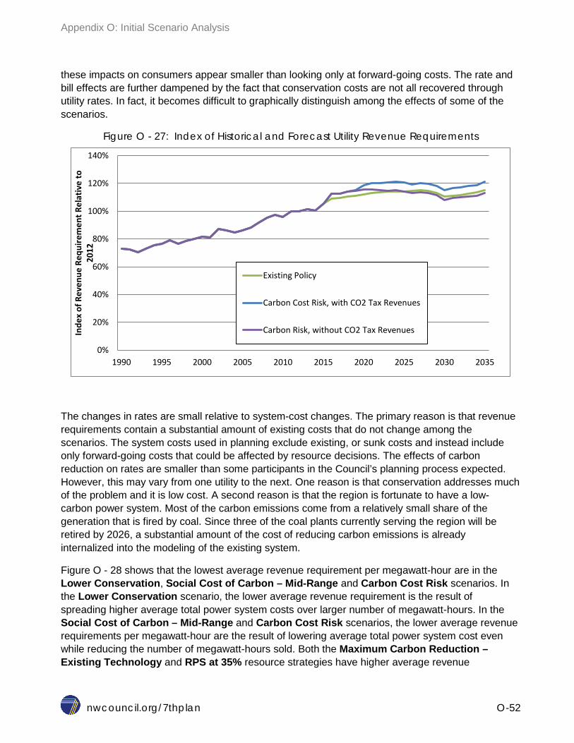
Appendix O: Initial Scenario Analysis
nwcouncil.org/7thplan O-52
these impacts on consumers appear smaller than looking only at forward-going costs. The rate and bill effects are further dampened by the fact that conservation costs are not all recovered through utility rates. In fact, it becomes difficult to graphically distinguish among the effects of some of the scenarios.
Figure O - 27: Index of Historical and Forecast Utility Revenue Requirements
The changes in rates are small relative to system-cost changes. The primary reason is that revenue requirements contain a substantial amount of existing costs that do not change among the scenarios. The system costs used in planning exclude existing, or sunk costs and instead include only forward-going costs that could be affected by resource decisions. The effects of carbon reduction on rates are smaller than some participants in the Council’s planning process expected. However, this may vary from one utility to the next. One reason is that conservation addresses much of the problem and it is low cost. A second reason is that the region is fortunate to have a low-carbon power system. Most of the carbon emissions come from a relatively small share of the generation that is fired by coal. Since three of the coal plants currently serving the region will be retired by 2026, a substantial amount of the cost of reducing carbon emissions is already internalized into the modeling of the existing system.
Figure O - 28 shows that the lowest average revenue requirement per megawatt-hour are in the Lower Conservation, Social Cost of Carbon – Mid-Range and Carbon Cost Risk scenarios. In the Lower Conservation scenario, the lower average revenue requirement is the result of spreading higher average total power system costs over larger number of megawatt-hours. In the Social Cost of Carbon – Mid-Range and Carbon Cost Risk scenarios, the lower average revenue requirements per megawatt-hour are the result of lowering average total power system cost even while reducing the number of megawatt-hours sold. Both the Maximum Carbon Reduction – Existing Technology and RPS at 35% resource strategies have higher average revenue
0%
20%
40%
60%
80%
100%
120%
140%
1990 1995 2000 2005 2010 2015 2020 2025 2030 2035
Inde
x of
Rev
enue
Req
uire
men
t Rel
ativ
e to
20
12
Existing Policy
Carbon Cost Risk, with CO2 Tax Revenues
Carbon Risk, without CO2 Tax Revenues
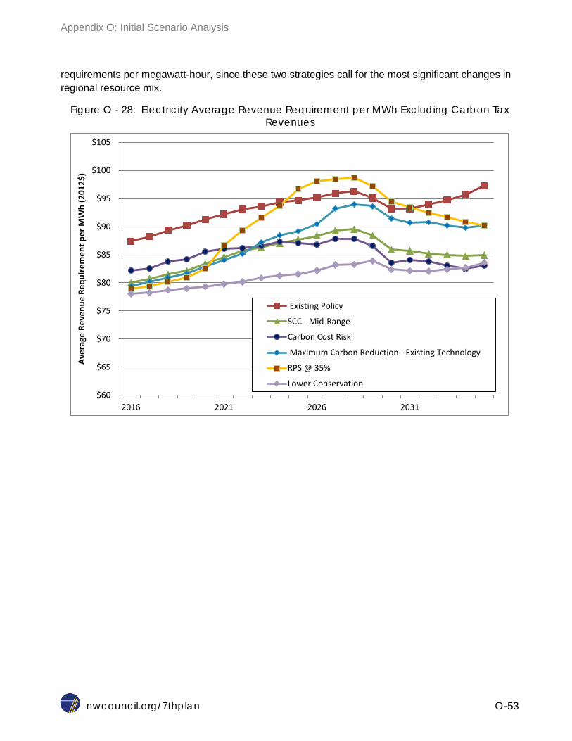
Appendix O: Initial Scenario Analysis
nwcouncil.org/7thplan O-53
requirements per megawatt-hour, since these two strategies call for the most significant changes in regional resource mix.
Figure O - 28: Electricity Average Revenue Requirement per MWh Excluding Carbon Tax Revenues
$60
$65
$70
$75
$80
$85
$90
$95
$100
$105
2016 2021 2026 2031
Aver
age
Reve
nue
Requ
irem
ent p
er M
Wh
(201
2$)
Existing Policy
SCC - Mid-Range
Carbon Cost Risk
Maximum Carbon Reduction - Existing Technology
RPS @ 35%
Lower Conservation

Seventh Northwest Conservation and Electric Power Plan
nwcouncil.org/7thplan P-1
APPENDIX P: GLOSSARY
COMMON ACRONYMS Acronym Meaning
aMW Average megawatt
ARM Adequacy Reserve Margin
ASCC Associated System Capacity Contribution
Btu
CHP
CCCT
British thermal unit
Combined heat and power
Combined cycle combustion turbine
DHP Ductless heat pumps
DOE Department of Energy
DSI Direct Service Industry
EPA Environmental Protection Agency
ETO Energy Trust of Oregon
FERC Federal Energy Regulatory Commission
GWh Gigawatt-hour
HRSG Heat recovery steam generator
IECC International Energy Conservation Code
IOU Investor-owned utility
IPP Independent power producer
ITC Investment tax credit
kWh Kilowatt-hour

Appendix P: Glossary
nwcouncil.org/7thplan P-2
LCOE Levelized cost of energy
LED lighting Light-emitting diode - solid state lighting
MCS
MWh
NEEA
Model Conservation Standards
Megawatt-hour
Northwest Energy Efficiency Alliance
NEI
NERC
Non-energy impacts
North American Electric Reliability Corporation
NPV
NREL
Net present value
National Renewable Energy Lab
NTTG Northern Tier Transmission Group
O&M
PTC
PUD
Operation and Maintenance
Production Tax Credit
Public Utility District
PURPA Public Utility Regulatory Policies Act of 1978
PV Photovoltaics
REC
RPM
Renewable energy credit
Regional Portfolio Model
RPS Renewable portfolio standards
RTF Regional Technical Forum
SHGC Solar heat gain coefficient
SMR
TEPPC
Small modular reactor
Transmission Expansion Planning Policy Committee
TRC Total resource cost
VRF Variable refrigerant flow
WECC Western Electricity Coordinating Council
WEPT Web-enabled programmable thermostats
Appendix P: Glossary
nwcouncil.org/7thplan P-3
Glossary of Terms adequacy To be considered adequate under the NERC definition, “the electric system [must be able to] supply the aggregate electrical demand and energy requirements of the customers at all times, taking into account scheduled and reasonably expected unscheduled outages of system elements.”
adequacy reserve margins A multiplier to peak or average load in the Regional Portfolio Model that reflects if more or less resources are required, in comparison to load resource balance, to meet the Council’s adequacy standard.
administrative costs
Certain overhead costs related to conservation or generating resources, such as project management and accounting costs incurred by utility or contractor staff.
alternating current (AC) An electric current in which the electrons flow in alternate directions. In North American electrical grids, this reversal of flow is governed at 60 cycles per second (Hertz). With some exceptions (see “direct current”), commercial electric generation, transmission and distribution systems operate on alternating current.
anadromous fish
Fish that hatch in freshwater, migrate to the ocean, mature there, and return to freshwater to spawn. For example, salmon or steelhead trout.
associated system capacity contribution The percent of a new resource’s capacity that contributes toward meeting the Council’s adequacy standard.
available technology
In the Power Plan, the term “available technology” refers to equipment or facilities for generating and conservation resources, including electrical appliances, that currently are available and are expected to be generally available in the marketplace during the 20-year planning period.
average cost pricing
A concept used in pricing electricity. The average cost price is derived by dividing the total cost of production by the total number of units sold in the same period to obtain an average unit cost. This unit cost is then directly applied as a price.

Appendix P: Glossary
nwcouncil.org/7thplan P-4
average megawatt (aMW) or average annual megawatt Equivalent to the energy produced by the continuous operation of one megawatt of capacity over a period of one year. (Equivalent to 8.76 gigawatt-hours, 8,760 megawatt-hours, or 8,760,000 kilowatt-hours.)
avoided cost An investment guideline, describing the value of conservation and generation resource investments in terms of the cost of more expensive resources that would otherwise have to be acquired.
balancing reserve Balancing reserves are provided by resources with sufficiently fast ramp rates to meet the second-to-second and minute-to-minute variations between load and generation left over after providing regulation and scheduled operations.
baseline efficiency The energy use of the baseline equipment, process, or practice that is being replaced by a more efficient approach to providing the same energy service. It is used to determine the energy savings obtained by the more efficient approach.
base-loaded resources
Base-loaded electricity generating resources are those that generally are operated continually except for maintenance and unscheduled outages. For example, hydroelectric, natural gas combined cycle combustion turbines, and coal plants.
billing credit Under the Northwest Power Act, a payment by Bonneville to a customer (in cash or offsets against billings) for actions taken by that customer to reduce Bonneville's obligations to acquire new resources.
Bonneville Power Administration (Bonneville) A federal agency that markets the power produced by Federal Base System resources and resources acquired under the provisions of the Northwest Power Act of 1980. Bonneville sells power to public and private utilities, direct-service industrial customers and various public agencies. The Northwest Power Act charges Bonneville with other duties, including pursuing conservation, acquiring sufficient resources to meet its contract obligations, funding certain fish and wildlife recovery efforts, and implementing the Council’s Power Plan and Fish and Wildlife Program.
Btu (British thermal unit) The amount of heat energy necessary to raise the temperature of one pound of water one degree Fahrenheit (3,413 Btus are equal to one kilowatt-hour).

Appendix P: Glossary
nwcouncil.org/7thplan P-5
busbar The physical electrical connection between the generator and transmission system. Typically load on the system is measured at busbar.
callback
A power sale contract provision that gives the seller the right to stop delivery of power to the buyer when it is needed to meet other specified obligations of the seller.
capacity
The maximum power that a machine or system can produce or carry under specified conditions. The capacity of generating equipment is generally expressed in kilowatts or megawatts. In terms of transmission lines, capacity refers to the maximum load a line is capable of carrying under specified conditions.
capacity factor An estimate of the ratio of the actual annual output to the potential annual output of a generating plant if operating at full capacity.
climate zone
As part of its model conservation standards, the Council has established climate zones for the region based on the number of heating degree days, as follows: Zone 1: 4,000 to 6,000 heating degree days (the mild maritime climate west of the Cascades and other temperate areas); Zone 2: 6,000 to 7,500 heating degree days (the somewhat harsher eastern parts of the region); and Zone 3: more than 7,500 heating degree days (western Montana and higher elevations throughout the region).
coal gasification
The process of converting coal to a synthetic gaseous fuel.
cogeneration
The sequential production of electricity and useful thermal energy. This is frequently accomplished by the recovery of excess heat from an electric generating plant for use in industrial processes, space or water heating applications. Conversely, cogeneration can be accomplished by using excess heat from industrial processes to power an electricity generator.
combined-cycle combustion turbine
The combination of a gas turbine and a steam turbine in an electric generation plant. The waste heat from the gas turbine provides the heat energy for the steam turbine.
Appendix P: Glossary
nwcouncil.org/7thplan P-6
conductor Wire or cable for transferring electric power.
conservation
According to the Northwest Power Act, any reduction in electric power consumption as a result of increases in the efficiency of energy use, production or distribution.
conservation program An activity, strategy, or course of action undertaken by an implementer or program administrator. Each program is defined by a unique combination of the program strategy, market segment, marketing approach, and energy-efficiency measure(s) included.
construction lead time
The length of time between a decision to construct a resource and when the resource is expected to deliver power to the grid. Generally defined for purposes of this plan as the interval between detailed engineering and equipment order to completion of start-up testing.
cost-effective
According to the Northwest Power Act, a cost-effective measure or resource must be forecast to be reliable and available within the time it is needed, and to meet or reduce electrical power demand of consumers at an estimated incremental system cost no greater than that of the least-costly, similarly reliable and available alternative or combination of alternatives.
cost of debt The amount paid to the holders of debt (bonds and other securities) for use of their money. Generally expressed as an annual percentage in the Power Plan.
cost of equity
Earnings expected by a shareholder on an investment in a company. Generally expressed as an annual percentage in this plan.
critical period
The sequence of historical low-water conditions during which the regional hydropower system’s lowest amount of energy can be generated (see “critical water”) while drafting storage reservoirs from full to empty to meet the Northwest’s loads. Under the Pacific Northwest Coordination Agreement, critical period is based on the lowest multi-month streamflow observed since 1928. The current critical period begins in October of 1936 and ends in September of 1937. A repeat of this historical water condition would generate about 11,600 average megawatts of hydroelectric energy.

Appendix P: Glossary
nwcouncil.org/7thplan P-7
current practice baseline
The baseline is defined by the typical choices of eligible end users in purchasing new equipment and services.
curtailment An externally imposed reduction of energy consumption due to a shortage of resources.
debt Investment funds raised through the sale of securities having fixed rates of interest.
debt/equity ratio
The ratio of debt financing to equity financing used for capital investment.
demand forecast An estimate of the level of energy that is likely to be needed at some time in the future. The Council’s demand forecast contains a range of estimated consumption based on various assumptions about demographics and the state of the economy.
demand response A voluntary and temporary change in consumers’ use of electricity when the power system is stressed.
direct application renewable resource
Technologies that use renewable energy sources to perform a task without converting the energy into electricity. These sources and their functions may include wood for space heat, solar for space heat and drying, geothermal space and water heating, and wind machines used for mechanical drive (such as pumping).
direct current (DC) An electrical current in which the electrons flow continuously in one direction. Direct current is used in specialized applications in commercial electric generation and in transmission and distribution systems.
direct-service industry (DSI) An industrial customer that buys power directly from the Bonneville Power Administration. Most direct-service industries are aluminum smelting plants.
discount rate
The rate used in a formula to convert future costs or benefits to their present value.

Appendix P: Glossary
nwcouncil.org/7thplan P-8
dispatch
Operating control of an integrated electrical system involving operations such as control of the operation of high-voltage lines, substations or other equipment.
distribution
The transfer of electricity from the transmission network to the consumer. Distribution systems generally include the equipment to transfer power from the substation to the customer’s meter.
drawdown
Release of water from a reservoir for purposes of power generation, flood control, irrigation, or other water-management activity.
economic feasibility
The Northwest Power Act requires all conservation measures to be “economically feasible” for consumers. The Act does not define this concept. In this plan, the Council considers a program or measure to be economically feasible if the measure or program results in the minimum life-cycle costs to the consumer, taking into account financial assistance, such as loans, grants, or other incentives, made available pursuant to other provisions of the Act.
end-use
A term referring to the final use of energy; it often refers to the specific energy services (for example, space heating), or the type of energy-consuming equipment (for example, motors).
energy
Energy is defined as a quantity of work, commonly measured in units of kilowatt-hours or megawatt-hours. In the Northwest, energy is also measured in units of average megawatts, where one average megawatt is equal to 8,760 megawatt-hours.
energy efficiency See conservation
energy-efficiency measure
Refers to either an individual project conducted or technology implemented to reduce the consumption of energy at the same or an improved level of service. Often referred to as simply a “measure”.
energy services
The actual service energy is used to provide (for example, space heat, refrigeration, transportation).
Appendix P: Glossary
nwcouncil.org/7thplan P-9
equity
Investment funds raised through the sale of shares of company ownership.
equivalent availability
The ratio of the maximum amount of energy a generating unit can produce in a fixed period of time, after adjustment for expected maintenance and forced outage, to the maximum energy it could produce if it ran continuously over the fixed time period. This represents an upper limit for a long-run (annual or longer) capacity factor for a generating unit. For example, a unit with an equivalent availability of 70 percent and a capacity of 500 megawatts could be relied on to produce 350 average megawatts of energy over the long term, if required.
externality
Any costs or benefits of goods or services that are not accounted for in the price of the goods or services. Specifically, the term given to the effects of pollution and other environmental effects from power plants or conservation measures.
Federal Base System
The system includes the Federal Columbia River Power System hydroelectric projects, resources acquired by the Bonneville Power Administration under long-term contracts prior to the Northwest Power Act, and resources acquired to replace reductions in the capability of existing resources subsequent to the Act.
Federal Energy Regulatory Commission (FERC) A federal agency that regulates interstate aspects of electric power and natural gas industries. It has jurisdiction over licensing of hydropower projects and setting rates for electricity sold between states. FERC formerly was the Federal Power Commission.
firm capacity
That portion of a customer’s capacity requirements for which service is assured by the utility provider.
firm energy
That portion of a customer’s energy load for which service is assured by the utility provider. That portion for which service is not assured is referred to as “interruptible.”
firm energy load carrying capability (FELCC) The amount of firm energy that can be produced from a hydropower system based on the system’s lowest recorded sequence of streamflows and the maximum amount of reservoir storage currently available to the system.
Appendix P: Glossary
nwcouncil.org/7thplan P-10
firm surplus
Firm energy in excess of the firm load.
first year cost of saved energy
The initial cost of implementing an energy-efficiency measure divided by the annual savings
fixed O&M cost An estimate of the fixed operation and maintenance cost for the reference plant, including operating and maintenance, labor and materials, and administrative overhead. Both routine maintenance, and major maintenance and capital replacement are assumed to be included.
flexibility Flexibility often refers to the ability of a power system to provide balancing reserves.
forecast of demand or load
Estimating future demand for electricity (measured at the customer meter site) or load (measured at busbar at the interconnection point of generation and transmission). The difference between demand and load forecasts are mainly transmission and distribution losses.
fuel cycle
The series of steps required to produce electricity from power plants. The fuel cycle includes mining or otherwise acquiring the raw fuel source, processing and cleaning the fuel, transporting, generating, waste management, and plant decommissioning.
futures Circumstances over which the decision maker has no control that will affect the outcome of decisions. For example, futures consists of unique combinations of natural gas and electricity prices, population and economic growth, none of which are within the control of resource planners.
gas turbine
A turbine engine generator, often fired by natural gas or fuel oil, used to generate electricity. The turbine generator is turned by combustion gases rather than heat-created steam.
generation
The act or process of producing electricity from other forms of energy.

Appendix P: Glossary
nwcouncil.org/7thplan P-11
geothermal energy
Thermal energy stored in the Earth’s crust. Geothermal heat is caused by the convection and conduction of heat from the Earth’s mantle and core, and from the decay of radioactive elements in the crust.
head
The vertical height of water in a reservoir above the turbine.
heat rate
The amount of input (fuel) energy required by a power plant to produce one kilowatt-hour of electrical output. Expressed as Btu/kWh.
heating degree days
A measure of the amount of heat needed in a building over a fixed period of time, usually a year. Heating degree days per day are calculated by subtracting from a fixed temperature the average temperature over the day. Historically, the fixed temperature has been set at 65 degrees Fahrenheit, the outdoor temperature below which heat was typically needed. As an example, a day with an average temperature of 45 degrees Fahrenheit would have 20 heating degree days, assuming a base of 65 degrees Fahrenheit.
higher heating value (HHV) / lower heating value (LHV) Gas turbine heat rates and efficiency ratings may be based on the HHV or LHV value of natural gas fuels. The HHV value of natural gas fuel may be thought of as the Btu content which was paid for, and includes content that is not convertible into power. Depending on the hydrogen content of the fuel, a rule of thumb is that 11 % of natural gas HHV Btu-content is not useful for power generation. The LHV is the HHV minus the heat of vaporization of the water vapor combustion product.
hydroelectric power (hydropower) The generation of electricity using falling water to turn turbo-electric generators.
incremental annual savings The difference between the amount of energy savings acquired or planned to be acquired as a result of energy efficiency activities in one year, and the amount of energy savings acquired or planned to be acquired as a result of the energy efficiency activities in the prior year.
incremental cost The difference between the cost of baseline equipment or service and the cost of alternative energy-efficient equipment or service.
Appendix P: Glossary
nwcouncil.org/7thplan P-12
independent power producer (IPP) An independent power producer is a power-production facility that is not part of a regulated utility. Power-production facilities that qualify under PURPA (see “qualifying facility”) are considered independent power producers, together with other independent power production facilities such as independently owned coal-fired and wind generating plants.
infiltration control Conservation measures, such as caulking and weatherstripping, generally referred to as air sealing measures, which reduce the amount of cold air entering or warm air escaping from a building.
insolation
The rate of energy from the sun falling on the earth’s surface, typically measured in watts per square meter.
integrated resource planning
See “least-cost planning.”
interruptible power Power that, by contract, can be interrupted in the event of a power deficiency.
intertie
A transmission line or system of lines permitting a flow of electricity between major power systems.
investor-owned utility (IOU) A utility that is organized under state law as a corporation to provide electric power service and earn a profit for its stockholders.
kilowatt (kW) The electrical unit of power that equals 1,000 watts.
kilowatt-hour (kWh) A basic unit of electrical energy that equals one kilowatt of power applied for one hour.
lead time The length of time it takes to move a resource from concept to completion.

Appendix P: Glossary
nwcouncil.org/7thplan P-13
least-cost planning
Least-cost planning or, as it is often called, “integrated resource planning,” is a name given to the Power Planning strategy and philosophy adopted by the Council. This strategy recognizes load uncertainty, embodies an emphasis on risk management, and reviews all available and reliable resources to meet current and future loads. The term “least-cost” refers to all costs, including capital, labor, fuel, maintenance, decommissioning, known environmental impacts, and difficult-to-quantify ramifications of selecting one resource over another.
levelized cost of energy (LCOE) The present value of a resource’s cost (including capital, financing, and operating costs) converted into a stream of equal annual payments. This stream of payments can be converted to a unit cost of energy by dividing them by the number of kilowatt-hours produced or saved by the resource in associated years. By levelizing costs, resources with different lifetimes and generating capabilities can be compared.
life-cycle costs Estimate of all direct costs of a measure or resource over its effective life. See system cost.
load
The amount of electric power required at a given point on a system. Load is typically measured at the busbar.
load forecast An estimate of the level of energy that must be generated to meet a need. This differs from a demand forecast in that transmission and distribution losses from the generator to the customer are included.
load path
One future scenario for electric load growth, as opposed to a range that accommodates multiple forecasts of future load growth.
lost-opportunity resources
Resources that, because of physical or institutional characteristics, can only be captured during a limited window of opportunity and are no longer available for development after that window at that given cost. For example, when a building is built or when a replacement refrigerator is purchased.
major resource
According to the Northwest Power Act, a resource with a planned capability greater than 50 average megawatts and, if acquired by Bonneville, acquired for more than five years.

Appendix P: Glossary
nwcouncil.org/7thplan P-14
manufactured home
A structure, such as a mobile home, that is transportable in one or more sections, and that is built on a permanent chassis and designed to be used as a dwelling, with or without a permanent foundation, when connected to the required utilities. These homes must comply with the Manufactured Home Construction and Safety Standards issued by the U.S. Department of Housing and Urban Development. This does not include other categories of homes whose components are manufactured, such as modular, sectional, panelized and pre-cut homes. These homes must comply with state and local building codes.
marginal cost The cost of producing the last unit of energy (the long-run incremental cost of production). In the plan, “regional marginal cost” means the long-run cost of additional consumption to the region due to additional resources being required. It does not include consideration of such additional costs to any specific utility due to its purchases from Bonneville at average cost.
maximum achievable potential The amount of energy or demand savings within a defined geographical area or population that can be achieved over the planning period assuming no financial barriers for the end-use customer.
measure
See energy-efficiency measure.
megawatt (MW) The electrical unit of power that equals one million watts or one thousand kilowatts.
megawatt-hour (MWh) A basic unit of electrical energy that equals one megawatt of power applied for one hour.
MicroFin A financial revenue requirements model that calculates the levelized fixed cost and the full levelized cost of energy (LCOE) for each resource reference plant. MicroFin calculates the annual cash flows which will satisfy revenue requirements over the plant lifetime. The annual cash flows are compressed and discounted into a dollar value – net present value (NPV).
Mid-C price/market price
The price of electricity traded on the wholesale spot market at the Mid-Columbia trading hub.
mill A tenth of a cent. The cost of electricity is often given in mills per kilowatt-hour.

Appendix P: Glossary
nwcouncil.org/7thplan P-15
model conservation standards (MCS) Any energy-efficiency program or standard adopted by the Council, including, but not limited to: 1) new and existing structures; 2) utility, customer, and governmental programs; and 3) other consumer actions for achieving conservation. The most well-known are the energy-efficient building standards developed by the Council for new electrically heated buildings.
Monte Carlo simulation
The mathematical simulation of uncertain events having known probability characteristics by random sampling from a known probability distribution function.
natural replacement Equipment or systems that are replaced at the end of their life are considered a natural replacement opportunities. At this time, there is an opportunity to replace the equipment or system with a more efficient alternative, and are considered lost opportunities resources.
net billed plants
Refers to the 30-percent share of the Trojan Nuclear Plant, all of Washington Public Power Supply System’s nuclear project 1 (WNP-1) and WNP-2, and 70 percent of WNP-3.
net billing
A financial arrangement that allowed Bonneville to underwrite the costs of electric generating projects. Utilities that owned shares in thermal projects, and paid a share of their costs, assigned to Bonneville all or part of the generating capability of these resources. Bonneville, in turn, credited and continues to credit the wholesale power bills of these utilities to cover the costs of their shares in the thermal resources. Bonneville then sells the output of the thermal plants, averaging the higher costs of the thermal power with lower-cost hydropower.
nominal dollars
Dollars that include the effects of inflation. These are dollars that, at the time they are spent, have no adjustments made for the amount of inflation that has affected their value over time.
non-energy impacts (NEI) The quantifiable non-energy impacts associated with program implementation or participation; also referred to as non-energy benefits (NEBs) or co-benefits. Examples of NEIs include water savings, non-energy consumables and other quantifiable effects. The value is most often positive, but may also be negative (e.g., the cost of additional maintenance associated with a sophisticated, energy-efficient control system).
Appendix P: Glossary
nwcouncil.org/7thplan P-16
non-firm energy
Energy produced by the hydropower system that is available with water conditions better than critical and after reservoir refill is assured. It is available in varying amounts depending upon season and weather conditions.
non-utility generator A generic term for non-utility Power Plan owners and operators. Non-utility generators include qualifying facilities, small power producers, and independent power producers.
Northwest Power Act Passed by Congress on December 5, 1980, the Pacific Northwest Electric Power Planning and Conservation Act authorized the four states of Idaho, Montana, Oregon and Washington to form the Northwest Power and Conservation Council. The Act directs the Council to assure the Pacific Northwest region an adequate, efficient, economical and reliable power supply while also protecting, mitigating and enhancing fish and wildlife affected by the construction and operation of hydroelectric dams in the Columbia River Basin. The Act requires the Council develop a 20-year Pacific Northwest conservation and electric power plan which the Council reviews at least every five years. The Act also requires the Council develop a fish and wildlife program to protect, mitigate and enhance fish and wildlife affected by the region’s hydrosystem and to include that program in the Council’s subsequently developed power plan.
option
As used in the Power Plan, a project that has been sited, licensed and designed, but not yet constructed. Options are held in inventory until new resources are clearly needed.
overnight capital cost Total of all direct and indirect project construction costs, including engineering, overhead costs, fees, and contingency. Exclusive of costs attributable to interest and escalation incurred during construction.
Pacific Northwest (the region) According to the Northwest Power Act, the area consisting of Oregon, Washington, Idaho, and Montana west of the Continental Divide, and those portions of Nevada, Utah, and Wyoming that are within the Columbia River Basin. It also includes any contiguous areas not more than 75 miles from the above areas that are part of the service area of a rural electric cooperative served by Bonneville on the effective date of the Act and whose distribution system serves both within and outside of the region.

Appendix P: Glossary
nwcouncil.org/7thplan P-17
Pacific Northwest Coordination Agreement An agreement between federal and nonfederal owners of hydropower generation on the Columbia River system. It governs the seasonal release of stored water to obtain the maximum usable energy subject to other uses.
peak (on, off, winter, summer) WECC defines peak-load hours to be the 16 hours beginning at 6am and ending at 10pm. Off-peak hours are the remaining eight hours in the day. For Council analysis, the winter period is roughly defined as the months of October through March. The summer period runs from April through September. However, the most important months with respect to resource planning are December, January and February. Similarly, the most critical summer months for resource planning are July and August.
peak capacity
The maximum capacity of a system to meet loads.
peak demand
The highest demand for power during a stated period of time.
penetration rate
One annual share of a potential market for conservation that is realized, as in “7 percent of the region’s homes have been weatherized this year.” Thus, a 7-percent penetration rate.
photovoltaic (PV) Direct conversion of sunlight to electric energy through the effects of solar radiation on semi-conductor materials.
potential assessments
Studies conducted to assess market baselines, future savings and costs that may be expected for different technologies and customer markets over a specified time horizon.
power Power is the rate of performing work, usually measured in units of kilowatts or megawatts.
preference
Priority access to federal power by public bodies and cooperatives.

Appendix P: Glossary
nwcouncil.org/7thplan P-18
present value
The worth of future returns or costs in terms of their current value. To obtain a present value, an interest rate is used to discount these future returns and costs.
ProCost A Council model used to estimate conservation costs and benefits; the hourly, daily, and seasonal savings; and capacity impact of efficiency measures.
program administration cost The cost incurred by the program administrator (often the utility) to deliver a conservation program. These costs include personnel, marketing, tracking systems, and any other non-incentive costs.
public utility commissions (PUC) State agencies that regulate, among others, investor-owned utilities operating in the state with a protected monopoly to supply power in assigned service territories.
Public Utility Regulatory Policies Act of 1978 (PURPA) Federal legislation that requires utilities to purchase electricity from qualified independent power producers at a price that reflects what the utilities would have to pay for the construction of new generating resources (see “avoided cost”). The Act was designed to encourage the development of small-scale cogeneration and renewable resources.
qualifying facility (QF) Qualifying facility is a power production facility that qualifies for special treatment under a 1978 federal law—Public Utility Regulatory Policies Act (PURPA). PURPA requires a utility to buy the power produced by the qualifying facility at a price equal to that which the utility would otherwise pay if it were to build its own Power Plant or buy the power from another source. A qualifying facility must generate its power using cogeneration, biomass, waste, geothermal energy, or renewable resources such as solar and wind, and, depending on the energy source and the time at which the facility is constructed, its size may be limited to 80 megawatts or smaller. PURPA prohibits utilities from owning majority interest in qualifying facilities.
quantifiable environmental costs and benefits
Environmental costs and benefits capable of being expressed in numeric terms (for example, in dollars, deaths, reductions in crop yields).
quartile
The direct-service industries load is divided into four quartiles. The top quartile is the portion of that load most susceptible to interruption.

Appendix P: Glossary
nwcouncil.org/7thplan P-19
R-value
A measure of a material’s resistance to heat flow. The higher the R-value, the higher the insulating value.
ramp rate (energy efficiency) The annual rate of acquisition for energy-efficiency resources over a period of time.
real dollars
Dollars that do not include the effects of inflation. They represent constant purchasing power.
reference plant A collection of characteristics that describe a resource technology and its theoretical application in the region.
region
See “Pacific Northwest.”
regional act credit Used in the act to give economic preference to conservation resources. When estimating incremental cost of an energy-efficiency measure, this cost is reduced by 10% of the value of the energy system benefits.
Regional Portfolio Model (RPM) An agent based planning model that develops least cost or least risk resource strategies for the regional power system. The model uses embedded Monte Carlo simulations to generate load, peak demand, natural gas price, carbon tax, electricity price, and REC value distributions allow resource strategies to be tested over many potential futures.
resource strategies
Actions and policies over which the decision maker has control that will affect the outcome of decisions. For example, the resource type, amount and potential timing of resource development.
reliability
Under the NERC definition, a power system is reliable if it is adequate and secure.
– adequate: the electric system can supply the aggregate electrical demand and energy requirements of the customers at all times, taking into account scheduled and reasonably expected unscheduled outages of system elements.
– secure: the electric system can withstand sudden disturbances, such as electric short circuits or unanticipated loss of system elements.

Appendix P: Glossary
nwcouncil.org/7thplan P-20
renewable energy credit (REC) Represent the “green” attribute of energy produced by a qualifying renewable resource. One REC is equal to one megawatt hour of generation. Also known as renewable energy certificate, or a tradeable renewable energy credit (TREC).
renewable resource
Under the Northwest Power Act, a resource that uses solar, wind, water (hydropower), geothermal, biomass, or similar sources of energy, and that either is used for electric power generation or for reducing the electric power requirements of a customer.
renewable portfolio standards Regulatory mandates enacted by individual states to increase the development and generation of eligible renewable resources. An RPS requires a certain percentage of electricity sales be met with renewable energy resources. In the Pacific Northwest, Montana, Washington, and Oregon all enacted RPS in the mid-2000’s.
reserve capacity
Generating capacity available to meet unanticipated demands for power, or to generate power in the event of outages in normal generating capacity. This includes delays in operations of new scheduled generation. Forced outage reserves apply to those reserves intended to replace power lost by accident or breakdown of equipment. Load growth reserves are those reserves intended for use as a cushion to meet unanticipated load growth.
resource
Under the Northwest Power Act, electric power, including the actual or planned electric capability of generating facilities, or actual or planned load reduction resulting from direct application of a renewable resource by a consumer, or from a conservation measure.
retrofit To modify an existing generating plant, structure, or process. The modifications are done to improve energy efficiency, reduce environmental impacts, or to otherwise improve the facility.
scenario Combinations of resource strategies and futures that are used to “stress test” how well what resource strategies (what the region controls) performs in a futures that the region doesn’t.
sectors
The economy is divided into four sectors for energy planning. These are the residential, commercial (e.g., retail stores, office and institutional buildings), industrial, and agriculture (e.g. dairy farms, irrigation) sectors.

Appendix P: Glossary
nwcouncil.org/7thplan P-21
sensitivity study A subset of scenario where a single input assumption is modified to assess the direction and magnitude of the impact of that parameter on the outcome. For example, fixing the range of natural gas prices to a lower or higher bound.
simple payback
The time required before savings from a particular investment offset costs, calculated by investment cost divided by value of savings (in dollars). For example, an investment costing $100 and resulting in a savings of $25 each year would be said to have a simple payback of four years. Simple paybacks do not account for future cost escalation, nor other investment opportunities.
siting agencies State agencies with the authority for issuing permits to locate generating plants of defined types and sizes to utilities at specific locations.
siting and licensing
The process of preparing a power plant and associated services, such as transmission lines, for construction and operation. Steps include locating a site, developing the design, conducting a feasibility study, preliminary engineering, meeting applicable regulatory requirements, and obtaining the necessary licenses and permits for construction of the facilities.
space conditioning
Controlling the conditions inside a building in order to maintain human comfort and other desired environmental conditions through heating, cooling, humidification, dehumidification, and air-quality modifications.
stock
The quantity and characteristics of existing equipment or buildings in the region.
sunk cost A cost already incurred and therefore not considered in making a current investment decision.
supply curve
A traditional economic tool used to depict the amount of a product available across a range of prices.
surcharge
Under the Northwest Power Act, an additional sum added to the usual wholesale power rate charged to a utility customer of Bonneville to recover costs incurred by Bonneville due to the failure of that customer (or of a state or local government served by that customer) to achieve conservation
Appendix P: Glossary
nwcouncil.org/7thplan P-22
savings comparable to those achievable under the Council’s model conservation standards. Surcharges can range from 10 to 50 percent of a customer’s bill.
system cost According to the Northwest Power Act, all direct costs of a measure or resource over its effective life. It includes, if applicable, distribution and transmission costs, waste disposal costs, end-of-cycle costs, fuel costs (including projected increases) and quantifiable environmental measures. The Council is also required to take into account projected resource operations based on appropriate historical experience with similar measures or resources.
technical potential (energy efficiency) An estimate of energy savings based on the assumption that all existing equipment or measures will be replaced with the most efficient equipment or measure that is both available and technically feasible over a defined time horizon, without regard to cost or market acceptance.
thermal resource
A facility that produces electricity by using a heat engine to power an electric generator. The heat may be supplied by burning coal, oil, natural gas, biomass, or other fuel, by nuclear fission, or by solar or geothermal sources.
tipping fee
The fee assessed for disposal of waste. This fee is used when estimating the cost of producing electricity from municipal solid waste.
total resource cost (TRC) test A cost-effectiveness test that assesses the impacts of a portfolio of energy-efficiency initiatives regardless of who pays the costs or who receives the benefits. The test compares the present value of costs of efficiency for all members of society (including all costs to participants and program administrators) compared to the present value of all quantifiable benefits, including avoided energy supply and demand costs and non-energy impacts.
transformer A device for transferring energy from one circuit to another in an alternating-current system. Its most frequent use in power systems is for changing voltage levels.
transmission
The act or process of long-distance transport of electric energy, generally accomplished by elevating the electric current to high voltages. In the Pacific Northwest, Bonneville operates a majority of the high-voltage, long-distance transmission lines.

Appendix P: Glossary
nwcouncil.org/7thplan P-23
turnover rate The portion of existing units that will be naturally replaced each year due to failure, remodeling, or renovation. It is usually calculated as one divided by the equipment average service life. Under the assumption that if equipment lasts for 10 years, one- tenth of the units in existence will be replaced each year. This factor is not used in the retrofit market, where inefficient equipment is replaced before its natural life is over. Nor is it used for new construction analyses, where all new equipment is eligible for efficiency upgrade at the time of purchase.
u-value
The measure of a material’s ability to conduct heat, numerically equal to 1 divided by the R-value of the material.
variable energy resource A generating resource that is non-dispatchable due to the fluctuating nature of its energy production. For example, windpower and solar.
variable O&M cost An estimate of the variable operation and maintenance cost for the reference plant, including all costs that are a function of the amount of power produced. This includes consumables such as water, chemicals, lubricants, and catalysts, and waste disposal.
watt The electrical unit of power or rate of energy transfer. One horsepower is equivalent to approximately 746 watts.

Appendix P: Glossary
nwcouncil.org/7thplan P-24
COUNCIL ADVISORY COMMITTEES The Council utilizes advisory committees to assist in the review of technical analysis and strategies. All advisory committees, with the exception of the Regional Technical Forum, are chartered under the Federal Advisory Committee Act (FACA). Advisory committee members are appointed by the Council and make up a diverse group of subject experts. All advisory committee meetings are open to the public.
Conservation Resources Advisory Committee (CRAC) Reviews policies and programs to assess how much energy efficiency is available and cost-effective.
Demand Forecasting Advisory Committee (DFAC) Reviews the methods, demand forecasting tools, input assumptions, and forecast results, used in developing the Council’s demand forecasts.
Generating Resources Advisory Committee (GRAC) Assists in the identification and review of generating resource and energy storage technologies, focusing on technical specifications, costs, and environmental effects.
Natural Gas Advisory Committee (NGAC) Reviews the Councils fuel price forecasting assumptions and models for natural gas, oil, and coal.
Regional Technical Forum (RTF) The RTF is an advisory committee to the Council established in 1999 to develop standards to verify, evaluate, and report conservation savings.
Resource Adequacy Advisory Committee (RAAC) Defines and assesses power supply adequacy and related issues.
Resource Strategies Advisory Committee (RSAC) Reviews the methods, key assumptions, and other major analytical inputs used in developing the resource plan.
System Analysis Advisory Committee (SAAC) Reviews the Council’s computer models and provides advice on their development.