Sexual Activity and the Lifespan of Male Fruitflies

Exploring, Organizing, and Describing, Quantitative Data

Essentials: Quantitative DataKnow this stuff - (stuff: a useful filler term in stats.)

Characteristics of quantitative variables.

Building a quantitative frequency table. From within a quantitative frequency table,

be able to identify: classes, class widths, class midpoints, class limits, boundaries (cutpoints)

Identify and construct appropriate charts/graphs for quantitative data.

EXPLORING, ORGANIZING, DESCRIBING, AND COMPARING DATA

Before beginning to analyze data, it is important to know three things:

1. Did the data come from a sample or a population?

2. Is the data qualitative or quantitative? 3. In what measurement scale is the data

reported?

Important Characteristics of a Data Set

Center – an “average” value that indicates where the middle of the data is located.

Variation – a measure of the amount that the values vary among themselves.

Distribution – the “shape” of the distribution of data.

Outliers – values that are far away from the majority of values.

Time – changing characteristics of data over time.

FREQUENCY DISTRIBUTIONS

A Frequency Distribution represents the range over which a variable’s values occur.

A Frequency Table lists classes (or categories) of values, along with the frequencies (counts) of the number of values that fall into each class. In addition, a frequency table may show cumulative frequencies, relative frequencies, and cumulative relative frequencies.

Frequency Tables are derived from RAW DATA and a TALLY process.

Quantitative Frequency Table Terms

Class – a grouping of data values Lower Class Limits – the smallest number

belonging to a class. Upper Class Limits – the largest number

belonging to a class. Class Boundaries – numbers used to separate

classes without the gaps created by class limits. (Also referred to as Cutpoints)

Class Midpoints – the midpoints of the classes. Class Width – the difference between two

consecutive lower class limits or lower class boundaries.

Quantitative Frequency Distributions

Grouped Frequency Distributions include a series of consecutive values into a Class (grouping)

Discrete or Continuous data may be presented

Ungrouped (or Single-Value) Frequency Distributions contain a Class (grouping) for each value of the variable

Generally, a small number of Discrete values are presented

Ungrouped or Single-Value Data Example

Data for: Number of School-Age Children

Single-Value Grouped Data Table

Each value is represented as a class.

Frequency Table of a Quantitative Variable(Grouped Data Example)

Old Faithful (length of time in minutes, between eruptions for 200 observations)

TIME f _________rf___40-49 8 0.0450-59 44 0.2260-69 23 0.11570-79 6 0.0380-89 107 0.53590-99 11 0.055100-109 1 0.005Totals 200 1.00

Classes represent ranges of discrete or continuous values. Here the class values represent the Lower and Upper Class Limits.

Histograms

A way to graphically represent quantitative continuous data

Horizontal scale represents classes. Vertical scale represents frequencies or relative

frequencies. Heights of the bars correspond to the frequencies (or

relative frequencies). Bars are adjacent to each other. That is, there are no

gaps between bars, (as occurs with bar charts).

Histogram for Single Value Data

Note that each discrete value is represented by a bar equaling the value’s frequency or relative frequency and that the bars touch.

Children

4.03.02.01.00.0

Number of School-Aged Childern

Among 30 Families

Cou

nt

14

12

10

8

6

4

2

0

Std. Dev = 1.28

Mean = 1.2

N = 30.00

Here the class values are the midpoints of the bars.

44.5 54.5 64.5 74.5 84.5 94.5 104.5

0

50

100

Old Faithful (Minutes Between Eruptions)

Fre

qu

ency

Histogram of Old Faithful Data

Here the midpoints of the classes are presented.

Time between Eruptions of Old Faithful Geyser

(Continuous Data)

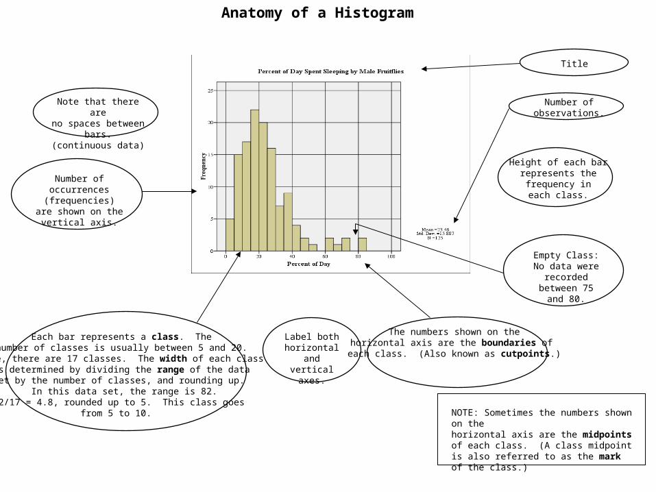
Anatomy of a Histogram

Title

Number ofoccurrences (frequencies)

are shown on thevertical axis.

Label bothhorizontal and

verticalaxes.

Height of each barrepresents thefrequency ineach class.

Note that there areno spaces between bars.

(continuous data)

Each bar represents a class. Thenumber of classes is usually between 5 and 20.

Here, there are 17 classes. The width of each classis determined by dividing the range of the dataset by the number of classes, and rounding up.

In this data set, the range is 82.82/17 = 4.8, rounded up to 5. This class goes

from 5 to 10.

The numbers shown on thehorizontal axis are the boundaries of

each class. (Also known as cutpoints.)

Number ofobservations.

Empty Class: No data were

recorded between 75 and 80.

NOTE: Sometimes the numbers shown on thehorizontal axis are the midpoints of each class. (A class midpoint is also referred to as the mark of the class.)

40 50 60 70 80 90 100

C1

Old Faithful(Length in min. between eruptions)

Dotplot

= Minutes

Here all 200 time periods are represented. In larger data sets each dot may represent multiple occurrences of a value.

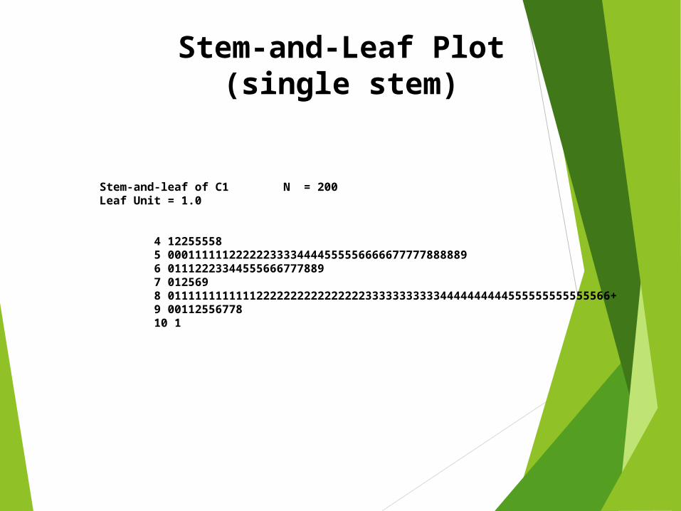
Stem-and-leaf of C1 N = 200Leaf Unit = 1.0

4 12255558 5 00011111122222233334444555556666677777888889 6 01112223344555666777889 7 012569 8 01111111111112222222222222222333333333334444444444555555555555566+ 9 00112556778 10 1

Stem-and-Leaf Plot (single stem)

Stem-and-Leaf (double stem)Stem-and-leaf of C1 N = 200Leaf Unit = 1.0

4 122 4 55558 5 00011111122222233334444 5 555556666677777888889 6 01112223344 6 555666777889 7 012 7 569 8 01111111111112222222222222222333333333334444444444 8 555555555555566666666666777777777777778888888888888888888 9 00112 9 556778 10 1

Old Faithful Data used for both stem-and-leafs

Percent of Day Spent Sleeping by Male Fruitflies        

   

1 8 12 17 20 23 28 35 66

2 9 13 17 20 24 28 36 71

4 9 13 17 20 24 29 36 73

4 9 14 17 21 24 29 37 81

4 9 14 17 21 25 29 37 83

5 10 14 17 22 25 30 38  

6 10 14 18 22 26 31 40  

6 10 15 18 22 26 31 40  

6 10 15 18 22 27 32 42  

6 10 15 18 22 27 32 43  

6 10 15 18 23 27 33 49  

6 12 15 18 23 27 34 49  

7 12 16 19 23 27 35 50  

8 12 16 19 23 28 35 62  

8 12 16 20 23 28 35 62  

Create a frequency table containing 9 classes, with the first lower class limit at 0.

80706050403020100

Male Fruitflies (percent of the day spent sleeping)

Male Fruitflies (percent of the day spent sleeping)

20 0 12444566666678889999 59 1 000000222223344445555566677777788888899 (36) 2 000011222223333334445566777778888999 30 3 0112234555566778 14 4 002399 8 5 0 7 6 226 4 7 13 2 8 13

Quantitative Presentations

1818 2020 2121 2727 2929 2020

1919 3030 3232 1919 3434 1919

2424 2929 1818 3737 3838 2222

3030 3939 3232 4444 3333 4646

5454 4949 1818 5151 2121 2121

The following data represents the ages of 30 students in a The following data represents the ages of 30 students in a statistics class. Construct a frequency distribution that has five statistics class. Construct a frequency distribution that has five classes. Graphically present these data as a histogram, stem-&-classes. Graphically present these data as a histogram, stem-&-leaf plot and a dot plot.leaf plot and a dot plot.

Ages of Students

End of Slides

<10 10 < 20 20 < 30 30 < 40 40 < 50 50 < 60 60 < 70 70 < 80 80 < 90

5

10

15

20

25

30

35

40

MALE FRUITFLIES(percent of the day spent sleeping)

n=125

Fre

quen

cy

Percent

Population Distribution

Sample Distribution

Stem-and-leaf of C1 N = 200Leaf Unit = 1.0

4 12255558 5 00011111122222233334444555556666677777888889 6 01112223344555666777889 7 012569 8 01111111111112222222222222222333333333334444444444555555555555566+ 9 00112556778 10 1

Stem-and-Leaf Plot(single stem)

Stem-and-leaf of C1 N = 200Leaf Unit = 1.0

4 122 4 55558 5 00011111122222233334444 5 555556666677777888889 6 01112223344 6 555666777889 7 012 7 569 8 01111111111112222222222222222333333333334444444444 8 555555555555566666666666777777777777778888888888888888888 9 00112 9 556778 10 1

Stem-and-Leaf(double stem)

Organizing Data Recall: a variable is a characteristic that varies from one person

or thing to another.

Frequency Distribution (fruitfly data) Lower Cutpoint Upper Cutpoint Midpoint Width

% f cf rf crf<10 20 20 0.16 0.16

10 < 20 39 59 0.312 0.47220 < 30 36 95 0.288 0.7630 < 40 16 111 0.128 0.88840 < 50 6 117 0.048 0.93650 < 60 1 118 0.008 0.94460 < 70 3 121 0.024 0.96870 < 80 2 123 0.016 0.98480 < 90 2 125 0.016 1Total 125 1