Simulating Turduckened Black Holes with a DiscontinuousGalerkin Scheme

Michael Wagman

Senior Honors Thesis for Mathematics-Physics ScB

Brown University Physics Department

Jan Hesthaven, Brown University Applied Math Department, Adviser

In this thesis we review how general relativity is reformulated to solve initial value

problems and discuss in particular the GBSSN system, a variant of the traditional

BSSN formulation commonly used in numerical relativity. We then construct a dis-

continuous Galerkin scheme for numerically solving the GBSSN system and describe

how to incorporate the turduckening technique for smoothing singularities in initial

data for black holes. We then present numerical simulations of a turduckened black

hole in spherical symmetry that build on the dG scheme used in [23] to simulate black

holes using excision, and we show that the robust stability and spectral convergence

of these simulations is maintained when we incorporate the turduckening technique.

A first order reduction of the GBSSN system is then presented along with the results

of numerical simulations using both excision, found to be stable and spectrally con-

vergent, and turduckening, found to be unstable with our present implementation.

Finally, we present a dG scheme for evolving a massless scalar field coupled to the

GBSSN system and discuss preliminary results showing the scheme allows for stable

simulations of the coupled system, in particular the infall and absorption of a scalar

field pulse by a black hole.

2

I. INTRODUCTION

General relativity, Einstein’s theory of gravity in which massive objects distort the geome-try of spacetime, has proven to be wildly successful at modeling a wide range of astrophysicalphenomena. In the early twentieth century, general relativity (GR) gained prominence byexplaining a well-known discrepancy between observation and Newtonian calculations forthe precession of Mercury’s orbit and famously predicting the correct deflection of starlightby the sun during a 1919 eclipse. Since then the quantitative accuracy of GR has been testedwith precision (see [47] for a review) and a number of often surprising general phenomenapredicted by the theory have been observed. Perhaps the most notable phenomenon is theexistence of black holes, objects so dense that the paths of all light rays inside a surfacesurrounding the black hole called the event horizon are bent so that they must travel in-wards towards the center of the black hole. Black holes are generically predicted to formwhen dense objects collapse under the pull of their own gravity, and there is a great dealof indirect observational evidence that astrophysical black holes do indeed exist, includingsupermassive black holes at the center of the Milky Way and other galaxies. See [7] for ahistory of black hole theory and observational evidence.

Direct tests of GR are often extremely difficult due to the weakness of gravity whencompared to the fundamental forces of particle physics; in “natural” units gravity is 1042

times weaker than electromagnetism. One important phenomenon predicted by GR is theexistence of gravitational waves, distortions in the curvature of spacetime and the distancebetween nearby points that propagate through space at a finite speed (in fact the speedof light) and obey the standard wave equation in the limit of weak gravitational coupling.By comparison Newtonian gravity couples all points in space at a fixed time–indeed theimpossibility of reconciling this fact with the fundamental postulate of special relativitythat information cannot travel faster then the speed of light already shows the need for avery different relativistic theory of gravity–and so Newtonian gravity does not allow for suchgravitational disturbances propagating at finite speed. Indirect evidence for gravitationalwaves has been provided by observations of binary pulsar systems, and measurements ofa decay in the orbital period of the Hulse Taylor Binary in agreement with the predictedenergy loss from gravitational wave emissions led to a 1993 Nobel prize [33].

Direct detection and measurements of gravitational waves would constitute importantevidence for this prediction and allow for precise tests of GR in the strongly coupled regimewhere detectable waves would be formed. Furthermore, because gravitational waves interactwith matter so weakly, waves formed in the early universe may look very similar todayto when they were emitted and the direct observation of gravitational waves may openuseful new avenues for early-universe astronomy. Experiments have been designed to detectgravitational waves through interferometry, and a new generation of upgraded detectors,most notably Advanced LIGO and Advanced Virgo, will be operational by 2015 and shouldbe sensitive enough to detect the gravitational waves emitted from the strongest predictedsources. Such sources should be very massive, not overly symmetric (in particular notaxisymmetric) systems whose gravitational profile varies significantly in time. The primeexample of such a source is a binary black hole system in which two nearby black holes collidethrough a process of three phases called inspiral, merger, and ringdown. The resulting blackhole will have less energy then the original dynamic binary black hole system with thedifference radiated away as gravitational waves. Highly accurate models of the gravitationalwaveforms that should be emitted by binary black hole systems and other strong sources

3

of gravitational waves are critical to successful experimental detection, as detectors rely ona process of matched filtering to separate potential signals from background noise. Thecurrent state of LIGO and Virgo and the quest for direct detection of gravitational waves isreviewed in [36].

Unfortunately there is no way to analytically calculate the details of a binary black holecollision. Apart from perturbative expansions useful only for weakly coupled systems, thereare no straightforward techniques for solving the equations of general relativity for a genericsystem. To get highly accurate predictions of gravitational waveforms, we are thereforeled to consider numerical simulations of binary black holes and other systems in generalrelativity. Such precise numerical simulations inevitably require costly computation, andgravitational wave detectors should ideally have a wide catalog of possible waveforms thatcan be compared to observed signals. It is therefore important to find a computationallyefficient numerical scheme whose accuracy increases quickly with increased computationalresolution.

Stable numerical simulations of binary black hole collisions have been successfully con-structed; the current state-of-the-art is reviewed in [42]. There are two main formulationsof GR that have been used in stable simulations: the generalized harmonic formulation andthe much more commonly used Baumgarte-Shapiro-Shibata-Nakamura (BSSN) formulation.Stable simulations for solving the BSSN system of partial differential equations (PDEs) haveby and large relied on finite difference schemes. Finite difference schemes provide a simplemeans of numerically approximating solutions to PDEs, but the numerical error in such ascheme only decreases with increasing spatial resolution as some power of the resolution.Recent work by Field, Hesthaven, Lau, and Mroue in [23] has proposed an alternative ap-proach for solving the BSSN system with a discontinuous Galerkin (dG) scheme in whichthe solution is approximated by local interpolating polynomials defined on subdomains thatcover the whole computational domain. A significant advantage of dG schemes is a propertyknown as spectral accuracy; the numerical error in the simulation decreases exponentiallywith increasing resolution. This high order accuracy, as well as robust stability in the pres-ence of shocks, make a dG scheme a competitive choice for performing binary black holesimulations.

The simulations in [23] and those presented here are both limited to the model problem ofevolving a single black hole in spherical symmetry for simplicity and relative computationalease. In the simulations in [23], the interior of the black hole’s event horizon is removedfrom the computational domain in order to avoid the singularity present at the center ofthe black hole using a technique called excision. Performing excision relies on knowing theprecise location of the event horizon of each black hole at all times. This means that binaryblock hole simulations with excision must include a computationally intensive process ofhorizon tracking, and state-of-the-art finite difference codes for solving the BSSN systemavoid using excision [42]. In this thesis we will describe a modification to the dG BSSNsimulations of Field et. al. in which the singularity is left in the computational domain butsmoothed out through a process known as turduckening [14, 15] and present results fromnumerical simulations with dG BSSN solver that use both excision and turduckening.

The structure of the thesis is as follows: Chapter II describes the basic ingredients ofGR, derives the ADM equations for formulating initial value problems in GR, and presentsa BSSN-type formulation called the Generalized BSSN (GBSSN) system that will be solvedin our numerical simulations. Chapter III provides a detailed description of dG methods anddescribes the construction of a scheme for solving the GBSSN system. Chapter IV describes

4

the construction of black hole initial data and the turduckening technique, the final elementsnecessary for building our simulations. The remaining chapters describe the results of ournumerical simulations. Chapter V describes numerical simulations of a static black holeusing a second order dG scheme and turduckening. Chapter VI describes simulations of afirst order reduction of the scheme using both excision and turduckening that have beenrecently published in [11]. Finally, chapter VII derives the equations for evolving a masslessscalar field coupled to the GBSSN system and describes some preliminary dG simulationsof a localized scalar field pulse falling into a black hole.

II. GENERAL RELATIVITY AND THE GBSSN EQUATIONS

This chapter begins with a brief overview of general relativity and the aspects of differen-tial geometry essential for understanding the Einstein field equations. The remainder of thechapter is devoted to reformulating the field equations in order to solve initial value prob-lems in GR. Section B introduces new variables that allow us to define a decomposition ofspacetime into a foliation of space-like hypersurfaces, Section C derives the ADM equationsthat reformulate the field equations in accordance with this decomposition, and Section Ddescribes the GBSSN system, a further reformulation of the ADM system better suited fornumerical evolution. The GBSSN system presented in Eq. (44) and Eq. (45) provides theconstraint and evolution equations used in the numerical simulations to follow.

A. General Relativity and Spacetime Covariance

In classical Newtonian physics, particles live in Euclidean 3-space with a single timeparameter agreed on by all observers throughout space. The combined spacetime is thereforedescribed by R3×R. Gravity is modeled as a force between massive objects that causes theirpaths to deviate from straight lines, the inertial trajectory of all particles. The situation isvery different in GR. Gravity distorts the structure of spacetime itself. Massive particles stilltravel along their inertial paths under the influence of gravity, but these paths themselvescurve in response to gravity.

To make this all precise, GR is described in the language of differential geometry. Space-time is only assumed to be an arbitrary 4-dimensional manifold M , a topological spacethat looks locally like flat space (more precisely, every point is contained in a neighborhooddiffeomorphic to a neighborhood of R4) but that may have a very different topological andgeometric character from that of Euclidean space R4. This manifold is equipped with asymmetric, non-degenerate inner product g(·, ·) called the metric1 that provides a way tomeasure the lengths and angles of vectors. M is called a pseudo-Riemannian manifold whenequipped with such a metric. The metric can by thought of as a generalization of the reg-

1 Important note on notation: the metric on M will be denoted by g and sometimes called the physical

metric to differentiate it from a metric γ defined on spatial slices of spacetime and a related metric g.

This final metric is the one that is actually taken as an evolved variable in the simulations that follow,

so we give it the simpler notation g. This makes the notation in this section a bit more cumbersome,

but will greatly streamline the notation in the remainder of the thesis. We adopt a (−,+,+,+) metric

convention throughout and will use geometrized units in which c = G = 1.

5

ular dot product in Euclidean space. Generalizing the idea of geometric tangent vectors tocurves and surfaces in R3, vectors are defined as elements of a vector space TpM called thetangent space that is constructed at every point p ∈ M . This tangent space can in fact berigorously defined as the collection of tangent vectors to all possible smooth curves passingthrough p ∈ M , that is directional derivative operators acting in all directions [38]. Linearmaps ω : TpM → R from vectors to the real numbers are called covectors and are describedas elements of the dual space T ∗pM . The metric g is a linear map TpM ⊗ TpM → R, thatis a bilinear map taking two vectors to the reals. It is called a rank (0,2) tensor, and wecan define tensors of arbitrary rank (p,q) as maps from p covectors and q vectors to thereal numbers. According to the principle of general covariance, all objects and equations ingeneral relativity are constructed using tensors to provide them with a geometric meaningthat does not depend on a particular observer’s choice of coordinate frame.

Choose coordinates (x0, x1, x2, x3) on some neighborhood of p ∈M , and define a coordi-nate basis for TpM by taking the directional derivative along each coordinate axis as a basisvector. For simplicity of notation we write ∂0 ≡ ∂

∂x0 , and so this coordinate basis is written∂0, ∂1, ∂2, ∂3. We will use index notation to describe vectors and covectors by their compo-nents in such a coordinate basis; for example we describe a vector v by vµ = (v0, v1, v2, v3)T

and a covector ω by ωµ = (ω0, ω1, ω2, ω3).2 We further adopt the Einstein summation con-vention in which all contractions, defined as repeated upper-lower index pairs, are summedover, for example vµωµ ≡

∑3µ=0 v

µωµ. A general tensor of rank (p, q) can be described by its

components Tµ1µ2...,µpν1ν2...,νq . Though the actual components of a tensor depend on the particular

choice of coordinates, equations relating tensors are covariant, that is they are independentof a particular choice of coordinates. The physical metric g is described by it’s componentsgµν . We further define an inverse metric gµν by gµνg

µρ = δρν where δνµ is the Kronecker delta,defined to be 1 if µ = ν and 0 otherwise. We can raise and lower indices using the metricand inverse metric, defining for example vµ ≡ gµνv

ν .Since derivatives like ∂µ obviously depend on the choice of coordinates, we look to define a

coordinate independent tensorial analog of the partial derivative called a covariant derivative.This covariant derivative is denoted by ∇µ and defined in the cases of vectors and covectorsby

∇µvν ≡ ∂µv

ν + Γν

µσvσ (1a)

∇µων ≡ ∂µων − Γσ

µνωσ, (1b)

where the connection Γµ

νλ is a (non-tensorial) set of functions defined by

Γµ

νλ ≡1

2gµσ(∂λgνσ + ∂νgλσ − ∂σgνλ). (2)

The covariant derivatives for tensors of higher rank are defined simply by adding anothercontraction of the connection with each raised index and subtracting a contraction of theconnection with each lower index. For a full discussion of manifolds, tensors, covariantderivatives, etc in the language of general relativity see [20, 45]; for a mathematical treatmentin the language of differential geometry see [21, 37, 38, 44].

2 Another important note on notation: Greek indices like µ and ν represent the four-dimensional spacetime

coordinates and will be assumed to run from 0 to 3, while Latin indices like i, j, k represent the three-

dimensional spatial coordinates only and will be assumed to run from 1 to 3.

6

The notion of curvature can be precisely defined on a (pseudo-Riemannian) manifold byconstructing the Riemann curvature tensor R

µ

νλρ as

Rµ

νλρ ≡ ∂λΓµ

νρ − ∂ρΓµ

νλ + Γµ

σλΓσ

νρ − Γµ

σρΓσ

νρ. (3)

Geometrically, Rµ

νλρ represents the change in the components of the coordinate vector ∂ρwhen it is parallel transported around an infinitesimal closed loop along in the plane of ∂νand ∂λ. We further define two contractions of the Riemann tensor called the Ricci tensorRµν and Ricci scalar R by

Rµν ≡ Rλ

µλν (4)

R ≡ Rµ

µ = gµνRµν . (5)

A manifold is called flat if and only if the Riemann tensor vanishes everywhere. Euclideanspace and the Minkowski space of special relativity are both flat since the metric in bothspaces is constant, diag(1, 1, 1, 1) for R4 and diag(−1, 1, 1, 1) for Minkowski space. In curvedspacetime it is no longer reasonable to postulate that the inertial path taken by particlesin the absence of an external force is a straight line defined by ∂2

t q(t, x) = 0, as can beseen by imagining a particle constrained to move along a sphere. Instead we postulate thatparticles travel along geodesics, paths that minimize the spacetime distance ds, defined byds2 ≡ gµνdx

µdxν , integrated along the path. Geodesics are equivalently paths that satisfy

the covariant generalization of straight-line paths ∇µdqdxν

= 0. Furthermore, light (and othermassless fields) travel along null geodesics, paths for which ds2 = 0. No causal informationcan travel faster than this, so the speed at which particles propagate along null geodesicsdefines the maximum speed of causal information flow.

The physical content of GR is given by the postulate that massive particles travel alongtime-like geodesics (geodesics where propagation is slower than light) and a description ofhow these geodesics are modified by the presence of other massive particles. Since thegeodesic equation can be written in terms of the components of the metric, this is equivalentto a statement of how the metric responds to the presence of mass. Such as statement isgiven by the Einstein field equations

Gµν ≡ Rµν −1

2Rgµν = 8πTµν , (6)

where Tµν is called the stress-energy tensor and characterizes the energy and momentum ofmatter throughout spacetime. It is defined and computed for a simple scalar field in ChapterVII. Note that in this equation and throughout this thesis we work in geometrized unitswhere G = c = 1.

The Einstein field equations above provide a system of 10 PDEs (the metric is symmetric,gµν = gνµ, and so areRµν and Tµν) for the physical metric components gµν in which each PDEinvolves non-linear products of the metric and its derivatives. While solving complicatednon-linear PDEs is not an easy task in general, there is an even more troubling feature ofthis system: spatial and time derivatives are mixed together in non-trivial combinations.This is a natural feature of GR since there is to be no distinction between space and timeapart from the sign of the metric and so any covariant equations must combine space andtime components equally. It contrasts sharply, however, with the notion of solving an initialvalue problem in which a system is described by a “snapshot” of its state at one point in

7

time and then evolved to determine its state at future times. This is exactly the kind ofproblem that numerical simulations are equipped to solve, and indeed the type of problemthat must be defined in order to model the gravitational waves emitted by a system startingin a specified binary black hole configuration.

Before we can begin describing a numerical scheme for solving Einstein’s equations, wewill need to re-formulate them as a system that describes the time evolution of the evolvedfields (gµν above) in terms of only the current state of the system at that point in time. Thisnecessarily requires that we distinguish between space and time, so we will now describehow to reformulate GR in a way that breaks spacetime covariance by singling out a timedirection but still maintains the physical content and the coordinate independence of thetheory.

B. Basic Elements of a Spacetime Decomposition

1. Lapse, Shift, and Spatial Metric

A fundamental assumption in GR is that spacetime is locally flat, as reflected in the ideathat we can choose local coordinates xµ mapping a neighborhood around any point to aneighborhood of R4. gµν is assumed to have signature +2, and so by purely linear algebraicconsiderations (see for example [35]) we can find coordinates in which it has a simple diagonalform at any given point. In particular we can choose coordinates so that at any given pointgµν = ηµν ≡ diag(−1, 1, 1, 1), the Minkowski metric of special relativity. In these coordinateswe can clearly distinguish the time coordinate x0. We can therefore foliate this local path ofspacetime by hypersurfaces Σt defined as level sets of the time coordinate t ≡ x0. As levelsets of a smooth function, these hypersurfaces will be 3-dimensional embedded submanifoldsof spacetime [38] and can be endowed with a spatial metric γij that acts on three-dimensionalvectors tangent to the hypersurface and describes the intrinsic geometry of the slice. Thisconstruction is non-covariant and can only be prescribed locally, but we follow [40] in usingit to build an intuition for the (tensorial) objects used to define a geometric decompositionof spacetime into space and time.

In order to describe the time evolution of the system we must relate the coordinate systemxi(t) on Σt with the coordinate system xi(t+ dt) on a surface Σt+dt an infinitesimal time dtin the future. To be precise, we look to choose xi(t + dt) so that a Eulerian observer [25],an observer whose worldline is orthogonal to Σt and so views events on the hypersurface assimultaneous, at a point pt ∈ Σt is described by the coordinates xi(d + dt) after moving intime to the point pt+dt ∈ Σt+dt. In flat spacetime this is simple. The Eulerian observer willalways move in the x0 direction, and so defining a time vector tµ = (1, 0, 0, 0), we may setthis vector equal to the unit normal vector for the hypersurface, nµ. Proper time will beequal to coordinate time, and the proper distance between the point pt ∈ Σt and an arbitrarypoint qt+dt ∈ Σt+dt will be ds2 = ηµνdx

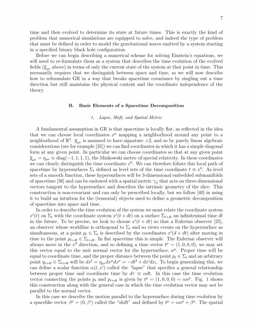
µdxν = −dt2 + dxidxi. To begin generalizing this, wecan define a scalar function α(t, xi) called the “lapse” that specifies a general relationshipbetween proper time and coordinate time by dτ ≡ αdt. In this case the time evolutionvector connecting the points pt and pt+dt is given by tµ = (1, 0, 0, 0) = αnµ. Fig. 1 showsthis construction along with the general case in which the time evolution vector may not beparallel to the normal vector.

In this case we describe the motion parallel to the hypersurface during time evolution bya spacelike vector βµ = (0, βi) called the “shift” and defined by tµ = αnµ + βµ. The spatial

8

FIG. 1. Diagrams describing the relations between the lapse α, shift β, normal vector nµ and

time vector tµ (note this time vector just gives the components of ∂t). The left diagram represents

flat space with coordinates chosen so that a Eulerian observer will measure zero spatial distance

between xi(t) and xi(t + dt), and the right diagram describes a curved spatial slice where the

Eulerian observer will measure a spatial shift between coordinates on the two slices.

distance between pt and an arbitrary qt+dt is then given by dxi +βidt. In terms of α, βi andthe spatial metric γij defined on Σt, the proper distance between arbitrary points on Σt andΣt+dt is given by

ds2 = gµνdxµdxµ = (−α2 + γijβ

iβj)dt2 + 2γijβidtdxj + γijdx

idxj. (7)

The components of the physical metric can immediately be read off from this equation, andinverting this 4x4 matrix gives the components of the inverse metric gµν . The metric andinverse metric are then given in block matrix form by

gµν =

(−α2 + γijβ

iβj γijβi

γijβj γij

), gµν =

(−1/α2 βj/α2

βi/α2 γij + βiβj/α2

). (8)

Since the physical metric gµν is fundamental to the spacetime manifold and defined inde-pendently of the choice of foliation, Eq. (7) may be viewed as a definition of α, β, andγij in terms of gµν . Furthermore, note that a choice of the fields α(t, xi) and βi(t, xi) justdefines a relation between coordinate distance and proper distance. The lapse and shiftare really gauge variables, and specifying a lapse and shift describes a particular choice ofcoordinates rather than specifying any physical information about the system. Also notethat the expression tµ = (1, 0, 0, 0) = αnµ + βµ for the time vector provides an expressionfor the normal vector in these coordinates given by

nµ =

(1

α,− 1

αβi). (9)

Finally, a bit more must be said about the spatial metric γ. In Eq. (7) only the spatialcomponents γij appear, but it will prove useful to extend the spatial metric to a tensorγµν that provides a map TpM ⊗ TpM → R rather than just TpΣt ⊗ TpΣt → R. This four-dimensional spatial metric should still only describe spatial distances and should obviouslyagree with γij for its spatial components. This can be accomplished by removing the lapseterms in gµν that represent the time distance between slices but keeping the shift terms that

9

represent the spatial distance traveled as time progresses, and so we define

γµν ≡ gµν + nµnν =

(γijβ

iβj γijβi

γijβj γij

). (10)

This tensor γµν also provides us with a operator that projects 4-dimensional vectors ontothe tangent space of each hypersurface TpΣt, as may be verified in the case of an arbitraryvector uν :

γνµuµ =

0

u1 + u0β1

u2 + u0β2

u3 + u0β3

. (11)

2. Intrinsic and Extrinsic Curvature

To finish describing our decomposition, we must be able to relate the curvature of Σt tothe spacetime curvature described by R

µ

νλρ. We can define a notion of intrinsic curvature

on Σt by building a connection Γijk and a Riemann curvature tensor Rijk` out of the spatial

metric γij since the hypersurface itself is a pseudo-Riemannian manifold. We can extendthese to be four-dimensional tensors by constructing them from γµν . In analogy to Eqs. (2)and (3), we define

Γµνλ ≡1

2γµσ(γνσ,λ + γλσ,ν − γνλ,σ) (12a)

Rµνλρ ≡ ∂λΓ

µνρ − ∂ρΓ

µνλ + ΓµσλΓ

σνρ − ΓµσρΓ

σνρ. (12b)

We can also build a covariant derivative operator Dµ using this connection in analogy to Eq.(1). This derivative operator can be verified to be the spatial projection of the spacetimecovariant derivative, that is Dµ = γνµ∇ν . It can also be directly verified that any component

of Rµνλρ with a 0 index will vanish, and so the spatial components of this tensor contain all

the relevant information for the intrinsic curvature [40].There is another notion of curvature called the “extrinsic curvature” of the submanifold.

To get some geometric intuition, consider a 2-dimensional cylinder embedded in R3. Sincea cylinder can be built by rolling up a flat piece of paper, it ought to have no intrinsiccurvature. This is indeed the case; since constructing such a cylindrical space is equivalentto taking cylindrical coordinates for flat Euclidean space the Riemann tensor defined on thecylinder will vanish. Still, a cylinder in some sense “looks curved” when viewed in R3. It isthis sense of curvature that is made precise by defining an extrinsic curvature tensor Kµν .

Consider an infinitesimal displacement dxi along a hypersurface Σt. The normal vectornµ(xi + dxi) will not in general be parallel to the normal vector nµ(xi), as is shown in Fig.2, and the one-form dnµ describing the difference between the two should be given by somelinear function of dxν . These two one forms will naturally then be related by a rank (1,1)tensor Kµ

ν . We therefore defineKij ≡ −∇inj. (13)

The extrinsic curvature tensor is symmetric, as will be verified shortly, and so we can replace∇inj with ∇(inj) ≡ 1

2(∇inj +∇jni) in the above definition. We wish the extrinsic curvature

10

FIG. 2. The normal vector nµ at points xν and xν +dxν on a curved hypersurface Σt. By historical

convention this surface is defined to have positive curvature. Since dnµ points opposite to dxν in

the diagram, we define Kµν to have a negative sign in its definition to respect this convention.

to be purely spatial, so we can define a four-dimensional tensor Kµν by taking a spatialprojection of the four-dimensional analog of this definition,

Kµν ≡ −γλµγρν∇(λ nρ). (14)

An equivalent and more computationally useful definition can be given in terms of a Liederivative of the spatial metric. The Lie derivative is a derivative operator that has anelegant definition for an arbitrary manifold without reference to a metric in terms of thetheory of flows along vector fields. For our purposes it can just be taken as a convenientshorthand for the combination of derivatives shown below, but it should be noted that allthe connection terms in its definition cancel and so any of ∂µ, ∇µ, or Dµ could equally wellbe used to take the Lie derivative. The definition of Kµν as a Lie derivative is seen to be

−1

2Lnγµν ≡ −

1

2

(nλDλγµν + γµλDνn

λ + γλνDµnλ)

(15)

= −1

2

(0 + γµλγ

σνg

λρ∇σnρ + γνλγσµg

λρ∇σnρ)

= −1

2γρµγ

σν

(∇σnρ +∇ρnσ

)= Kµν .

C. The ADM Formalism

The first reformulation of the Einstein field equations suitable for solving general initialvalue problems was provided by Arnowitt, Deser, and Misner in 1959 by deriving what arenow called the ADM equations [4]. These provide evolution equations for the spatial metricand extrinsic curvature as well as two constraint equations, purely spatial equations thatmust be satisfied on each hypersurface in the foliation. The structure of the equations issuch that so long as the constraint equations are satisfied by the initial data specified on aspatial surface at the initial time t = 0 they will be preserved by the evolution equationsand automatically satisfied at later times. We present a derivation of the ADM equationsvery different from the original and initially follow the approach of [40] before adopting themore abstract and fully covariant techniques of [9].

11

The ADM equations can be derived by combining the Einstein field equations with threeequations that relate the the extrinsic and intrinsic curvature of the hypersurfaces to thespacetime curvature: the Gauss, Codazzi, and Ricci equations. The spatial pieces of theGauss and Codazzi equations can be most easily derived by taking an orthogonal basis forour tangent space rather then the usual coordinate basis, so we will very briefly slip out ofindex notation and view for example the extrinsic curvature tensor K(·, ·) as an operatortaking two vectors as inputs.

Let fi be an orthonormal frame providing a basis for TpΣt, and let ei = (0, fi). Our normalvector n is orthogonal to the ei, so take n, ei as an orthogonal frame providing a basisfor TpM . Note that nµ is normalized so that g(n,n) = −1. We mentioned upon defining

the Riemann curvature tensor Rµ

νλρ that it could be interpreted as measuring the changeresulting from parallel transporting a vector around an infinitesimal closed loop. This ismade precise in an equivalent definition of the Riemann curvature tensor as

R (ei, ej, ek) = ∇ej∇ekei −∇ek∇ejei ≡ ∇j∇kei −∇k∇jei. (16)

The components of this resultant vector will give Rµ

ijk in terms of objects defined on the

hypersurface as we desire, so we look to resolve the components of ∇kei in the n, ei basis.To calculate the spatial components, note that by the orthogonality of ei and ej we have

∂jei = 0, and so ∇kei = Γ`ike`. This allows us to calculate the spatial components as

g(ej,∇kei) = Γ`jkg (e`, ei) = Γ`jkg`i = Γijk. (17)

The 0 (normal) component is given by

g(n,∇kei) = −g(ei,∇kn) = g(ei, ej)Kjk = gijK

jk = Kik, (18)

where the first equality follows from the orthogonality of ei and n and the important property∇λgµν = 0 called metric compatibility, as 0 = ∇kg (ei,n) = g

(∇kei,n

)+ g

(∇kn, ei

). At

this point we can easily verify that Kij is symmetric as was asserted before:

Kji = g(n,∇jei) = g(n, eµ)Γµij = g(n, eµ)Γµji = g(n,∇iej) = Kij. (19)

We can now express ∇kei in terms of the (n, ei) basis by

∇kei = g(n,∇kei

) n

g(n · n)+ g

(ej,∇kei

) ejg(ej, ej)

(20)

= −Kikn + Γ`ike`.

Applying a second covariant derivative operator gives

∇j∇kei = ∇j

(−Kikn + Γ`ike`

)= −∇jKikn +

(−KikK

`j +∇jΓ

`ik + ΓmikΓ

`mj

)e`. (21)

The second term of Eq. (16) is identical under an interchange of j and k, so we can nowexpress the spacetime Riemann curvature tensor in terms of the extrinsic curvature and theintrinsic Riemann curvature tensor on the hypersurface as

R (ei, ej, ek) =(∇kKij −∇jKik

)n +

(KijK

`k −KikK

`j + R`

ijk

)e`. (22)

12

The spatial piece of this equation decomposes the spatial curvature of the hypersurface intointrinsic and extrinsic parts and is known as Gauss’s equation,

R`

ijk = R`ijk +KikK

`j −KijK

`k , (23)

while the normal component describes how the extrinsic curvature changes throughout thefoliation and is known as Codazzi’s equation,

R0

ijk = ∇kKij −∇jKik. (24)

Rather than expressing these as spatial and normal components of the spacetime Riemanncurvature tensor, we can write them as projections of the full tensor onto the spatial andnormal directions. Gauss’s equation is equivalent to

γλµγδνγ

ησγ

ξρRλδηξ = Rµνσρ +KνρKµσ −KνσKµρ, (25)

and Codazzi’s equation can be expressed as

γηνγρσγ

ξµn

λRηρξλ = DσKµν −DνKµσ. (26)

The geometric structure of these equations as different projections of the Riemann curvaturetensor is clear. The symmetries of the Riemann tensor dictate that projecting all fourcomponents onto the normal direction will trivially vanish, but there is one further non-trivialrelation that can be found by projecting two components of Rµνλσ onto the hypersurfaceand two onto the normal direction. This relation is known as the Ricci equation, and isgiven by [9]

γδµγηνn

σnλRησδλ =1

αDµDνα +Kρ

νKµρ + LnKµν . (27)

The ADM constraint equations can be immediately derived from the Gauss and Codazziequations as they are expressed above. Contracting the left side of Gauss’s equation withγµσγνρ and performing a series of index manipulations gives 2nµnνGµν . This can be related tothe stress-energy tensor by the Einstein field equations. To express the constraint conciselywe define an energy density ρ by

ρ ≡ nµnνTµν . (28)

This has the physical interpretation of the energy density on the hypersurface as measured bya Eulerian observer. Combining the contracted form of Gauss’s equation with the Einsteinfield equations provides the Hamiltonian constraint

H ≡ R +K2 −KijKij = 16πρ. (29)

Contracting the left side of Codazzi’s equation with the spatial metric γνσ can be shown togive −γδµnλRδλ. Observing γδµn

λgδλ = nµ−nµ = 0, we can trivially add a term proportional

to gδλ and in particular can add 12Rγδµn

λgδλ so that this becomes a contraction of the Einstein

tensor Gδλ. For convenience we define this same contraction of the stress-energy tensor by

jµ ≡ −γδµnλTδλ. (30)

jµ can be interpreted as the momentum density measured by a Eulerian observer. Combiningthe Einstein field equations and the contracted Codazzi equation provides the momentumconstraint

Mi ≡ DjKji −DiK = 8πji. (31)

13

The remaining ADM equations are evolution equations for the spatial metric γij and extrinsiccurvature Kij. Recall the definition of the time vector tµ = αnµ + βµ that has componentstµ = (1, 0, 0, 0) in our coordinate basis. Since any x0 components of the spatial connectionΓµνρ will vanish, the Lie derivative along tµ reduces to simply the partial derivative ∂t in ourchosen coordinates. The Lie derivative can itself be thought of a linear operator taking avector and a tensor as input, and so Lt = αLn − Lβ [38].

The evolution equation for γij can therefore be found immediately by rearranging Eq.(15) to give

∂tγij = −2αKij − Lβγij. (32)

The evolution equation for Kµν can be found by rearranging the Ricci equation to solve forLnKµν and decomposing this Lie derivative as above to give [9]

∂tKij = −DiDjα− α(Rij − 2KikK

kj +KKij

)− 8πα

(Sij −

1

2γij(S − ρ)

)+ LβKij, (33)

where we have introduced a spatial projection of the stress energy tensor

Sµν ≡ γλµγρνTλρ, (34)

as well as the trace of this projection

S ≡ γµνSµν = γijSij. (35)

We finally define the trace-free part of this tensor by

STFij ≡ Sij −

1

3γijS. (36)

This will be featured in the next section.

D. The GBSSN System

The ADM evolution equations turn out to be poorly suited for numerical evolution3.Since the development of the ADM formalism, there have been numerous new formulationsproposed in an effort to find a system more suitable for numerical evolution. The mostpopular in modern numerical relativity simulations are the generalized harmonic system andthe BSSN system. There is even a range of systems described as BSSN-type formulations,see for example [8, 10, 12]. Our particular choice is commonly called the generalized BSSNor GBSSN formulation, and differs from the traditional BSSN formulation by defining all ofthe evolved fields to be tensors (except for one non-tensorial field related to the connection)rather than having some be objects known as tensor densities whose components pick upa weighted Jacobian factor when transformed to new coordinates. This is accomplished byremoving the restriction present in traditional BSSN that the evolved metric to has unitdeterminant, consequently making the reduction to spherical symmetry, where in flat space

3 More precisely they are only weakly hyperbolic when written in first order form [22], a condition that

causes many numerical schemes to become unstable or lose convergence [17].

14

the spatial metric has determinant r2, much simpler with GBSSN than with traditionalBSSN.

We begin by defining a conformal spatial metric gij and a conformal factor χ by

gij ≡ χγij, gij ≡ γij

χ(37)

The conformal factor χ is a scalar that effectively rescales the spatial metric and is usefulat least in spherical symmetry in isolating the divergences in the physical metric found atthe central singularity of a black hole from the evolved conformal metric. When the spatialmetric γij diverges, we can allow the conformal metric gij to remain finite so long as theconformal factor χ approaches zero. It is similarly useful to perform this same conformaldecomposition with the extrinsic curvature. Define the trace K and trace-free part Aij ofthe conformal extrinsic curvature by

Kij =1

χ

(Aij +

1

3gijK

). (38)

The trace K and trace-free part Aij are evolved separately as independent fields. Also definea connection built from conformal spatial metric gij by

Γijk ≡1

2gim(∂kgmj + ∂jgmk − ∂mgjk). (39)

Finally define conformal connection functions by contracting the conformal connection withthe spatial metric,

Γi ≡ gjkΓijk = − 1√g∂j(√

ggij). (40)

These conformal connection functions provide the final evolved variables for the GBSSNsystem. The full set of evolved variables in GBSSN are then the gauge variables α, βi, andBi, a vector to be introduced shortly in the evolution equations that introduces damping tothe shift vector, and the physical fields gij, Aij, K, Γi, and χ.

Evolution equations for the gauge variables may be chosen freely, but the numericalstability of the resulting scheme depends greatly on this choice. We use the “1+log” and“Γ-driver” conditions [1] common to nearly all stable binary black hole evolutions usingBSSN [42]. As can be seen from Eq. (37), there is also some ambiguity in determining theevolution equations for both the conformal factor and the conformal metric from the ADMevolution equation for the spatial metric. This ambiguity and a similar ambiguity resultingfrom conformal decomposition of the extrinsic curvature are resolved by explicitly specifyingthe evolution of the conformal metric determinant g. This provides the major distinctionbetween traditional BSSN formulations alluded to earlier: in traditional BSSN g = 1 for alltimes, while we specify a “Lagrangian condition” ∂t(ln g) = 0 [12].

All of the numerical simulations presented in this thesis are limited to spherically sym-metric spacetimes, so we will immediately specialize to this case. The spherically symmetricline element is given in terms of the evolved GBSSN variables by

ds2 =

(−α2 +

βr2grrχ

)dt2 +

2βrgrrχ

dtdr +grrχdr2 +

gθθχ

(dθ2 + sin2 θdφ2). (41)

15

Note that in these coordinates radially incoming and outgoing null geodesics, defined aspaths satisfying ds2 = 0, have coordinate velocity

dr

dt= −βr ± α

√χ

grr. (42)

Subject to spherical symmetry, the conformal connection and trace-free conformal extrinsiccurvature reduce to [23]

Γi =

Γr

− cos θgθθ sin θ

0

, Aij = Arr

1 0 00 − gθθ

2grr0

0 0 −gθθ sin2 θ2grr

. (43)

This means that in spherical symmetry our evolved fields are just α, βr, Br, grr, gθθ, Arr,K, Γr, and χ.

A full derivation of the spherically symmetric GBSSN evolution and constraint equationsfrom the ADM equations is presented in Appendix A of [22] using the choices describedabove for the evolution of the gauge variables and conformal metric determinant in notationidentical to that of this thesis except that conformal variables have bars instead of physicalvariables, so we will not repeat the calculation here. Using the ADM evolution equationsand the choices described above, the GBSSN evolution equations in spherical symmetry aregiven by

∂tα = βrα′ − 2αK − (∂tα)0 (44a)

∂tβr = βrβr′ +

3

4Br − (∂tβ

r)0 (44b)

∂tBr = βrBr′ + λ(∂tΓ

r − βrΓr′)− ηBr − (∂tBr)0 (44c)

∂tχ = βrχ′ +2

3Kαχ− βrg′rrχ

3grr− 2βrg′θθχ

3gθθ− 2

3βr′χ (44d)

∂tgrr =2

3βrg′rr +

4

3grrβ

r′ − 2Arrα−2grrβ

rg′θθ3gθθ

(44e)

∂tgθθ =1

3βrg′θθ +

Arrgθθα

grr− gθθβ

rg′rr3grr

− 2

3gθθβ

r′ (44f)

∂tArr = βrA′rr +4

3Arrβ

r′ − βrg′rrArr3grr

− 2βrg′θθArr3gθθ

+2αχ(g′rr)

2

3g2rr

− αχ(g′θθ)2

3g2θθ

(44g)

− α(χ′)2

6χ+

2

3grrαχΓr′ − αχg′rrg

′θθ

2grrgθθ+χg′rrα

′

3grr+χg′θθα

′

3gθθ− αg′rrχ

′

6grr− αg′θθχ

′

6gθθ

− 2

3α′χ′ +

αχ′′

3− 2

3χα′′ − αχg′′rr

3grr+αχg′′θθ3gθθ

− 2αA2rr

grr+KαArr −

2grrαχ

3gθθ− 8παχSTF

rr

∂tK = βrK ′ +χg′rrα

′

2g2rr

− χg′θθα′

grrgθθ+α′χ′

2grr− χα′′

grr+

3αA2rr

2g2rr

+1

3αK2 + 4πα(S + ρ) (44h)

∂tΓr = βrΓr′ +

Arrαg′θθ

g2rrgθθ

+2βr′g′θθ3grrgθθ

+Arrαg

′rr

g3rr

− 4αK ′

3grr− 2Arrα

′

g2rr

− 3Arrαχ′

g2rrχ

(44i)

+4βr′′

3grr− βr(g′θθ)

2

grrg2θθ

+βrg′′rr6g2

rr

+βrg′′θθ

3gθθgrr− 16παjr

χ,

16

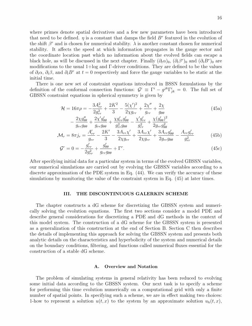
where primes denote spatial derivatives and a few new parameters have been introducedthat need to be defined. η is a constant that damps the field Br featured in the evolution ofthe shift βr and is chosen for numerical stability. λ is another constant chosen for numericalstability. It affects the speed at which information propagates in the gauge sector andthe coordinate location past which no information about the evolved fields can escape ablack hole, as will be discussed in the next chapter. Finally (∂tα)0, (∂tβ

r)0 and (∂tBr)0 are

modifications to the usual 1+log and Γ-driver conditions. They are defined to be the valuesof ∂tα, ∂tβ, and ∂tB

r at t = 0 respectively and force the gauge variables to be static at theinitial time.

There is one new set of constraint equations introduced in BSSN formulations by thedefinition of the conformal connection functions: Gi ≡ Γi − gjkΓijk = 0. The full set ofGBSSN constraint equations in spherical symmetry is given by

H = 16πρ = −3A2rr

2g2rr

+2K2

3− 5(χ′)2

2χgrr+

2χ′′

grr+

2χ

gθθ(45a)

− 2χg′′θθgrrgθθ

+2χ′g′θθgrrgθθ

+χg′rrg

′θθ

g2rrgθθ

− χ′g′rrg2rr

+χ(g′θθ)

2

2grrg2θθ

Mr = 8πjr =A′rrgrr− 2K ′

3− 3Arrχ

′

2χgrr+

3Arrχ′

2χgrr+

3Arrg′θθ

2grrgθθ− Arrg

′rr

g2rr

(45b)

Gr = 0 = − g′rr2g2

rr

+g′θθgrrgθθ

+ Γr. (45c)

After specifying initial data for a particular system in terms of the evolved GBSSN variables,our numerical simulations are carried out by evolving the GBSSN variables according to adiscrete approximation of the PDE system in Eq. (44). We can verify the accuracy of thesesimulations by monitoring the value of the constraint system in Eq. (45) at later times.

III. THE DISCONTINUOUS GALERKIN SCHEME

The chapter constructs a dG scheme for discretizing the GBSSN system and numeri-cally solving the evolution equations. The first two sections consider a model PDE anddescribe general considerations for discretizing a PDE and dG methods in the context ofthis model system. The construction of a dG scheme for the GBSSN system is presentedas a generalization of this construction at the end of Section B. Section C then describesthe details of implementing this approach for solving the GBSSN system and presents bothanalytic details on the characteristics and hyperbolicity of the system and numerical detailson the boundary conditions, filtering, and functions called numerical fluxes essential for theconstruction of a stable dG scheme.

A. Overview and Notation

The problem of simulating systems in general relativity has been reduced to evolvingsome initial data according to the GBSSN system. Our next task is to specify a schemefor performing this time evolution numerically on a computational grid with only a finitenumber of spatial points. In specifying such a scheme, we are in effect making two choices:1-how to represent a solution u(t, x) to the system by an approximate solution uh(t, x),

17

and 2-in what sense this approximate solution uh(t, x) will be made to satisfy the evolutionsystem. To discuss this concretely but without the complexity of the GBSSN system we willconsider a simple model system

∂u

∂t+∂f(u)

∂x= g(x) (46)

throughout this section and the next. In this equation u(t, x) is the solution to be determined,f(u) represents a spatial flux and g(x) acts as a (time-independent) source for the field u.An initial value problem is determined by specifying a spatial domain Ω on which we wishto solve the system, initial data u0 ≡ u(t = 0, x) defined for all x ∈ Ω, and some type ofboundary conditions for u on the boundary ∂Ω. Assume that Ω can be well-approximatedby a discrete computational domain Ωh. By specifying how to spatially discretize the systemas an equation for uh on x ∈ Ωh we will obtain a semi-discrete scheme for solving Eq. (46).We will then be left with an ordinary differential equation for the time evolution of thesystem at each of the finitely many spatial points in Ωh that can be discretized and solvedby well-known and understood methods.

The oldest and simplest approach for spatial discretization is the finite difference scheme.In a finite difference scheme Ωh is defined as a set of equally spaced grid points, Ωh ≡x1, x2..., xK. Denote the grid spacing by h ≡ xk+1 − xk. We construct the numericalsolution uh(t, x) by building local polynomials interpolating u(t, x) at the grid points. Forx ∈

[xk−1, xk+1

], define uh by

uh(t, x) ≡2∑i=0

ai(t)(x− xk)i. (47)

Discretized fluxes fh and source terms gh are defined analogously. To describe the mannerin which uh is chosen to satisfy the PDE, define the residual Rh by

Rh ≡∂uh∂t

+∂fh∂x− gh(x). (48)

The residual in effect measures the difference between the approximate and exact solutionand will in general be nonzero since uh(t, x) 6= u(t, x). The natural statement to enforcefor this scheme is that the residual vanish at each grid point x1, ..., xK . To define a (secondorder) finite difference scheme, we approximate the action of the spatial derivative operatorat a grid point by the difference quotient of the function at two the surrounding grid points.The time evolution of uh is then determined by enforcing that the residual vanish at eachgrid point to give

∂uh(xk, t)

∂t+fh(x

k+1, t)− fh(xk−1, t)

2h− gh(xk) = 0. (49)

While appealingly simple, there are drawbacks to the finite difference scheme, most no-tably a lack of geometric flexibility when constructing multidimensional grids and poorscaling of accuracy with resolution, as compared to dG and other methods in [32]. Tay-

lor expanding fh(xk+1) = fh(x

k + h) = fh(x) + hf ′(x) + h2

2f ′′(x) + O(h3) and fh(x

k−1) =

fh(xk − h) = fh(x

k) + hf ′(xk) + h2

2f ′′ + O(h3) and substituting these expressions into the

above equation shows that the error in making our finite difference approximation is O(h2);

18

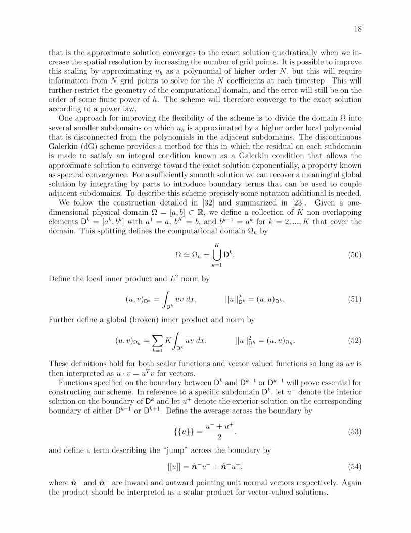
that is the approximate solution converges to the exact solution quadratically when we in-crease the spatial resolution by increasing the number of grid points. It is possible to improvethis scaling by approximating uh as a polynomial of higher order N , but this will requireinformation from N grid points to solve for the N coefficients at each timestep. This willfurther restrict the geometry of the computational domain, and the error will still be on theorder of some finite power of h. The scheme will therefore converge to the exact solutionaccording to a power law.

One approach for improving the flexibility of the scheme is to divide the domain Ω intoseveral smaller subdomains on which uh is approximated by a higher order local polynomialthat is disconnected from the polynomials in the adjacent subdomains. The discontinuousGalerkin (dG) scheme provides a method for this in which the residual on each subdomainis made to satisfy an integral condition known as a Galerkin condition that allows theapproximate solution to converge toward the exact solution exponentially, a property knownas spectral convergence. For a sufficiently smooth solution we can recover a meaningful globalsolution by integrating by parts to introduce boundary terms that can be used to coupleadjacent subdomains. To describe this scheme precisely some notation additional is needed.

We follow the construction detailed in [32] and summarized in [23]. Given a one-dimensional physical domain Ω = [a, b] ⊂ R, we define a collection of K non-overlappingelements Dk = [ak, bk] with a1 = a, bK = b, and bk−1 = ak for k = 2, ..., K that cover thedomain. This splitting defines the computational domain Ωh by

Ω ' Ωh =K⋃k=1

Dk. (50)

Define the local inner product and L2 norm by

(u, v)Dk =

∫Dkuv dx, ||u||2Dk = (u, u)Dk . (51)

Further define a global (broken) inner product and norm by

(u, v)Ωh =∑k=1

K

∫Dkuv dx, ||u||2Ωh = (u, u)Ωh . (52)

These definitions hold for both scalar functions and vector valued functions so long as uv isthen interpreted as u · v = uTv for vectors.

Functions specified on the boundary between Dk and Dk−1 or Dk+1 will prove essential forconstructing our scheme. In reference to a specific subdomain Dk, let u− denote the interiorsolution on the boundary of Dk and let u+ denote the exterior solution on the correspondingboundary of either Dk−1 or Dk+1. Define the average across the boundary by

u =u− + u+

2, (53)

and define a term describing the “jump” across the boundary by

[[u]] = n−u− + n+u+, (54)

where n− and n+ are inward and outward pointing unit normal vectors respectively. Againthe product should be interpreted as a scalar product for vector-valued solutions.

19

B. Constructing a Nodal dG Scheme

On each subdomain Dk we construct our approximate solution ukh as a local interpolatingpolynomial of specified order N

x ∈ Dk : ukh(t, x) ≡N∑i=0

ukh(t, xki )`

ki (x), (55)

where `kj is the jth Lagrange interpolating polynomial, defined in Dk by

`kj (x) ≡N∏i=0i 6=j

x− xkixkj − xki

. (56)

This polynomial interpolates the exact solution u at the nodes xkj . Within each subdo-

main Dk these are distributed as Legendre-Gauss-Lobotto nodes, defined as the roots of thepolynomial equation

(1− s2)P ′N(s) = 0, (57)

where PN is the Nth Legendre polynomial. To map these nodes to the computational grid,we define an affine mapping from the interval [−1, 1] to Dk by

xk(s) = ak +1

2(1 + s)(bk − ak). (58)

This allows us to define our nodal points as xkj = xk(sj). The global solution uh is formallydefined as

uh(t, x) ≡K⊕k=1

ukh(t, x). (59)

For each subdomain Dk, define a residual Rkh analogous to Eq. (48) by

Rkh ≡

∂ukh(t, x)

∂t+∂fkh (u)

∂x− gkh(x). (60)

This specifies a discrete approximate of the solution and brings us to the second choiceof how this approximate solution will be made to satisfy the PDE. The condition we willenforce is that the residual on each subdomain is orthogonal to a space of test functions onthe subdomain. Choosing these test functions to be the Lagrange interpolating polynomialstaken previously as our basis for ukh specifies what is called the kth Galerkin condition:

(Rkh, `

kj

)Dk

=

∫ bk

ak

(∂ukh(t, x)

∂t+∂fkh (u)

∂x− gkh(x)

)`j(x) dx = 0 ∀j. (61)

Apart from the analytically known interpolating polynomials `ki (x), the spatial dependenceof the polynomial approximations ukh, f

kh , and gkh is completely described by the values at

the N + 1 nodal points in each subdomain, and so these Galerkin conditions provide a setof K(N + 1) integral equations for the solution at each nodal point. This will become oursemi-discrete scheme, though there is as of yet no coupling between the solutions in each

20

subdomain. To provide this coupling we look to incorporate information from the boundaryof the subdomain into these integral conditions, and so we integrate the flux term by partsto give ∫ bk

ak

[∂ukh(t, x)

∂t`kj (x)− fkh (u)

∂`kj (x)

∂x− gkh(x)`kj (x)

]dx+

[fkh (u)`kj (x)

∣∣bkak

= 0. (62)

Rather than enforce this precise condition, we define a numerical flux f ∗h(u) that will incor-porate information from the subdomains adjacent to Dk and enforce∫ bk

ak

[∂ukh(t, x)

∂t`kj (x)− fkh (u)

∂`kj (x)

∂x− gkh(x)`kj (x)

]dx+

[f ∗h(u)`kj (x)

∣∣bkak

= 0. (63)

The numerical flux f ∗h is only featured in the boundary term of this expression and is thereforeonly defined on the boundaries of Dk. To provide the desired coupling between subdomainsit is defined to be a function of the interior and exterior solutions at each boundary, that isf ∗h = f ∗h(u+, u−). The stability of a dG scheme depends upon the choice of f ∗h , and we willdelay discussing the numerical fluxes chosen for solving the GBSSN system until the nextsection. Employing a second integration by parts provides the integral equations∫ bk

ak

(∂ukh(t, x)

∂t+∂fh(u)

∂x− gkh(x)

)`kj (x)dx+

[(f ∗h(u)− fh(u)) `kj (x)

∣∣bkak

= 0. (64)

This defines the form of the Galerkin conditions that we enforce.Note that solution u is approximated in Dk as an N -degree polynomial ukh and the source

g(x) can naturally be approximated as an N -degree polynomial gkh by defining a straightfor-ward analog of Eq. (55). If the flux f(u) contains any products of the form a(x)b(x), as thenonlinear GBSSN system certainly does, it would naturally be expressed as a polynomial ofdegree 2N or higher. In order to keep fh(x) in the span of our basis of degree N Lagrangepolynomials, we must replace any products of interpolated polynomials with interpolationsof the product function like

(a(t, x)b(t, x))kh = akh(t, x)bkh(t, x)→N∑i=0

ah(t, xki )bh(t, x

ki )`

ki (x). (65)

These two expressions are not equivalent and this interpolation of products results in whatis known as aliasing error. Aliasing error in dG is discussed in [32], and the next sectionintroduces an exponential filter to prevent any resulting aliasing-driven numerical instabili-ties. Using the above prescription any flux or source terms in an arbitrary non-linear PDEcan still be approximated by N -degree polynomials interpolated at the nodal points. Fur-thermore, since the nodal values of product functions are found by multiplying the nodalvalues of each factor pointwise, we need only consider the K(N + 1) nodal values for eachevolved variable.

We can therefore represent our solution ukh as a vector of its values at the nodal pointsby taking

ukh(t, x) = uk(t)T`k(x), (66)

where the vectors uk(t) and `k(x) are given by

uk(t) =[uk(t, xk0), ..., uk(t, xkN)

]T, `k(x) =

[`k0(x), ..., `kN(x)

]T, (67)

21

noting that at the nodal points uk(t, xki ) = ukh(t, xki ). In this representation, Eq. (64)

becomes a set of N + 1 ODEs for the coefficients uk(t) in each subdomain. Furthermore,since there is no spatial dependence in these coefficients themselves we can therefore carryout the spatial integration in Eq. (64) independently from the time integration. To thisend, define the mass and stiffness matrices Mk and Sk on the k-th subdomain by

Mkij =

∫ bk

akdx `ki (x)`kj (x), Skij =

∫ bk

akdx `ki (x)

∂`kj∂x

. (68)

Since spatial derivatives will only affect the nodal basis functions `k(x), we can also builda matrix Dk that acts as a numerical spatial derivative operator. In terms of the abovematrices this derivative matrix is given by

Dkij =∂`kj∂x

∣∣∣∣∣x=xki

=N+1∑m=1

(Mk

)−1

imSmj. (69)

We can now express the semi-discrete evolution equations in each subdomain as the matrixequation

∂tuk = Dkfk(uk) + gk +

(Mk

)−1`k[fk(uk)− f ∗(u+, u−)

∣∣bkak. (70)

Though throughout this section we have worked with the toy system given by Eq. (46),the construction of a nodal dG scheme for solving the GBSSN system is a straightforwardgeneralization. Each evolved variable is approximated by a local interpolating polynomialdefined on each subdomain, and the evolution equation for each evolved variable in Eq.(44) can be used to define a residual for that variable on each subdomain. By enforcing theGalerkin condition that the inner product of each residual with the N Lagrange interpolatingpolynomials that act as our basis functions and introducing a numerical flux for each field wecan form a discretized evolution equation. These will be close analogs to Eq. (70), thoughnow the flux and source vector analog of f(u) in each equation will be a functions of all theevolved fields.

There is one significant complication in constructing a dG scheme for solving the GBSSNsystem not present in our model system: the flux is assumed to be an algebraic function ofthe evolved system variables, but the GBSSN system includes second order spatial deriva-tives. This discrepancy is resolved by defining auxiliary variables representing the spatialderivatives of each field for which second derivatives appear. We define an auxiliary lapsefunction for example as Qα ≡ ∂rα. These auxiliary variables are not themselves evolved inthe second order scheme presented in [23] and used in many of the simulations to follow.They are instead computed from the evolved variables at each step of the time evolutionby defining a residual on the k-th subdomain for each auxiliary variable straight from itsdefinition. For Qα this residual is defined as

(RQα)kh = − (Qα)kh + ∂rαkh. (71)

As with the residuals defined by the evolution equations, we enforce a Galerkin condition((RQα)kh, `j

)kD

= 0 for all j and introduce a numerical flux α∗h(α+, α−) to solve for the nodal

values likeQα = Dkα+

(Mk

)−1`k [α∗ −α]b

k

ak , (72)

22

where we have suppressed the subdomain index k and any functional dependencies. In thefirst order scheme presented in Chapter VI, the auxiliary fields like Qα are promoted toindependently evolved system variables with their own discretized evolution equations inplace of the above equation.

The discrete evolution equations for the evolved fields in the GBSSN system can now beconstructed as analogs of Eq. (70) using the techniques of this section. As a representativeexample, the evolution equation for K is discretized as

∂tK = βrDkK − χDkQα

grr+χQgrrQα

2grr− χQgθθQα

grrgθθ

+QαQχ

2grr+

3αA2rr

2g2rr

+1

3αK2 + (Mk)−1`k [fK − f ∗K |

bk

ak . (73)

The index k is again suppressed, and products of vectors in this expression are to be inter-preted as pointwise products as described in Eq. (65).

We are now just left with an ordinary differential equation for the time evolution of eachevolved GBSSN variable at each grid point. Discretizing the time evolution is schematicallyaccomplished by calculating the change in each variable over a small but finite timestep∆t by substituting the field values at time t into the above semi-discrete equation and itsanalogs for the other variables, adding this change to find the fields at t+ ∆t, and iteratingthis process to find the fields at a desired later time. The simulations presented in this thesisuse a fourth-order Runge-Kutta method to perform the time evolution, a common choicefor performing time integration in computational physics and described in the context of adG scheme in [32]. Numerical stability depends upon the choice of timestep.

The last major general property of dG methods to be described is the convergence withpolynomial order N . A proof of the spectral convergence of dG methods is given in [32]; wewill simply sketch out the main points. From the properties of the Legendre polynomial Pj,it can be shown that any function u can be approximated by a weighted sum of the first NLegendre polynomials denoted u∗, the “best approximating polynomial of order N”, on thesubdomain Dk with an error bounded like

||u− u∗||Dk ≤ C(t)(hk)N+1, (74)

where hk is the length of Dk and C(t) is a (time-dependent) constant. An arbitrary nodalrepresentation unodal of u using the first N Lagrange interpolating polynomials can then beshown to approximate U with an error bounded like

maxx∈Dk|u− unodal| ≤ (1 + Λ) max

x∈Dk|u− u∗|, (75)

where the constant Λ depends only on the nodal points chosen. The Legendre-Gauss-Lobotto nodal points are defined precisely as the nodal points that minimize Λ, and so ourinterpolation error does not differ significantly from the error of the best approximatingpolynomial u∗. This allows us to bound the error of our nodal representation ukh like

||u− ukh||Dk ≤ C(t)(hk)N+1, (76)

where C(t) is a new time-dependent constant. This verifies that the error between the exactsolution and our numerical approximation decreases exponentially with N and so a nodal dGscheme possess spectral convergence. The error also depends on the size of the subdomains

23

and increasing the number of subdomains will decrease the numerical error as well, thoughthe convergence in this case may depend on the details of the subdomain construction andhow the numerical error is distributed through the domain.

Finally, this idea of approximating a function using a basis of Legendre polynomialsleads us to discuss an equivalent modal representation of the solution u that will be used inthe next section when we discuss filtering. We can express ukh(t, x) in a basis of Legendrepolynomials Pj(x) like

ukh(t, x) =N∑j=0

u(t, xkj )`kj (x) =

N∑j=0

ukj (t)Pj(x), (77)

where the ukj are called the modal coefficients of the system and can be calculated from theabove relation to the nodal representation. Modal coefficients for larger k correspond tothe coefficients of higher-order Legendre polynomials and therefore to the higher-frequencymodes of the solution.

C. Details of a dG Scheme for GBSSN

1. Wavespeeds and Characteristics

We first consider a few analytic properties of the GBSSN system relevant to our numericalsimulations, namely the characteristic variables and wavespeeds of the system and stronghyperbolicity, a necessary condition for the well-posedness of an initial problem. Theseare properties of the GBSSN system itself rather than of any particular discretization ofit. To carry out this analysis with a minimum of notational clutter, we define an abstractrepresentation of the GBSSN system using the column vectors

u =

χgrrgθθαβr

, v =

Br

ArrKΓr

, Q = u′ =

χ′

g′rrg′θθα′

βr′

, W =

uvQ

. (78)

Note that these are vectors of functions of the coordinates (t, r) rather than vectors of pointsin the computational domain as were considered previously. In particular W corresponds tothe solution u of the model system in the last section rather than the vector u of its valuesat nodal points. While in our second order simulations the auxiliary sector Q is constructedat each timestep, many theoretical tools for analysis of PDEs are developed only for fullyfirst order PDEs. In particular the notion of strong hyperbolicity of a second order systemis defined in the context of the strong hyperbolicity of possible first order reductions of thesystem. In this section we will therefore consider a first order reduction of GBSSN in which Qis independently evolved, found by making the replacements u′ → Q, u′′ → Q′ in the GBSSNsystem. For a detailed discussion of characteristics, hyperbolicity, boundary conditions, andassociated topics for second order systems in the context of numerical relativity see [27, 28].

In this notation we can write the GBSSN system as a matrix analog of the model systemgiven by Eq. (46). Since each term in Eq. (44) is linear in terms involving spatial derivatives

24

v′ and Q′ and the coefficients of these terms depend only on u, we can define a matrix A(u)and a source vector S(W ) to express the GBSSN system as

∂tW + A(u)W ′ = S(W ). (79)

In this notation the physical fluxes like fK are given by the corresponding components ofA(u)W . The homogeneous part of this equation, ∂tW + A(u)W ′ = 0 is called the principlepart of the equation.

If the matrix A(u) were diagonal, then the principle part of the system would de-couplethe fields so that each evolved variable would independently satisfy an equation analogousto the model system. So long as A(u) is diagonalizable, we can transform the solution vectorW into the eigenbasis of A(u) in which the flux has this simple form. The components of Win the eigenbasis of A(u) are called the characteristic variables of the system and denotedby Xi. The corresponding eigenvalues of A(u) are called the characteristic speeds, or moresuggestively wavespeeds, and will be denoted by µi with the set of eigenvalues denoted µ(A).Considering only the principle part of the system, the Xi satisfy ∂tXi = −µi∂rXi and so theydefine integral curves in the phase space of the system that a solution will move along withvelocity −µi as it evolves in time. When max |µ(A)| is larger, the area of the computationaldomain causally connected to a given point in a fixed length of time will be larger. Sincethe spatial resolution of a numerical scheme is fixed independently of the wavespeeds of thesystem, this suggests that a smaller timestep may be necessary to maintain stability, andthe choice of timestep in our numerical simulations is therefore guided by max |µ(A)|.

Since all instances of u′ in the GBSSN system have been replaced with Q, the upper-left 5x5 block of A(u) will be the zero matrix. This makes each field in u a characteristicvariable of the system with wavespeed 0. The remaining 9 characteristic variables andcorresponding wavespeeds are found by diagonalizing the non-degenerate 9x9 block of A(u).The eigenvalues of this block are given by

µ1 = 0, µ2 = −βr, µ3 = −βr,

µ±4 = −βr ±√

2αχgrr, µ±5 = −βr ± α

√χgrr, µ±6 = −βr ±

√λgrr.

(80)

The characteristic variables can be calculated by finding the matrix of eigenvalues used todiagonalize A(u) and then applying this matrix to the state vector W to give4

X1 = gθθQgrr + 2grrQgθθ , (81a)

X2 = grrΓr +

2

χQχ −

1

2grrQgrr

− 1

gθθQgθθ , (81b)

X3 =grrλBr +

2

χQχ −

1

2grrQgrr + χ− 1

gθθQgθθ , (81c)

X±4 = ±√

2αgrrχ

K +Qα, (81d)

4 This calculation is carried out in some detail in Appendix A of [23]. For a detailed description of the process

of finding the characteristic variables and wavespeeds for a simpler system and using them to construct

Sommerfeld boundary conditions, see our derivation of the characteristic variables for the Klein-Gordon

equation in section VII B 3

25

X±5 = ∓ 3√grrχ

Arr ± 2

√grrχK + 2grrΓ

r +1

χQχ −

1

grrQgrr +

1

gθθQgθθ , (81e)

X±6 = −3

4

grrλBr ± α

√λgrr

2αχ− λK − βr

8(βrgrr ∓

√λgrr

)Qgrr (81f)

− βrgrr

4gθθ(βrgrr ∓

√λgrr

)Qgθθ +αχ

2αχ− λQα ±

√grrλQβr .

It will further prove useful to express the evolved fields in v and Q in terms of u and thecharacteristic variables. Inverting the above system gives

Br =− 1

6

λ

grrgθθ

[(βr)2

(βr)2grr − λ

]X1 +

2λαχ

3grr(2αχ− λ)

(X+

4 +X−4)− 2λ

3grr

(X+

6 +X−6)(82a)

Arr =1

3

√grrχ

2α

(X+

4 −X−4)−√grrχ

6

(X+

5 −X−5)

(82b)

K =

√χ

8αgrr

(X+

4 −X−4)

(82c)

Γr =− 1

6grrgθθ

[(βr)2

(βr)2grr − λ

]X1 +

1

grr(X2 −X3) +

2αχ

3grr(2αχ− λ)

(X+

4 +X−4)

(82d)

− 2

3grr

(X+

6 +X−6)

Qχ =χ

12grrgθθ

[4(βr)2grr − 3λ

(βr)2grr − λ

]X1 +

χ

2X3 −

αχ2

3(2αχ− λ)

(X+

4 +X−4)

(82e)

+χ

3

(X+

6 +X−6)

Qgrr =2(βr)2grr − 3λ

6gθθ((βr)2grr − λ)X1 +

4

3grrX2 − grrX3 +

2αχgrr3(2αχ− λ)

(X+

4 +X−4)

(82f)

− 1

3grr(X+

5 +X−5)− 2

3grr(X+

6 +X−6)

Qgθθ =

[1

4grr+

(βr)2

12((βr)2grr − λ)

]X1 −

2

3gθθX2 +

1

2gθθX3 −

αχgθθ3(2αχ− λ)

(X+

4 +X−4)

(82g)

+1

6gθθ(X+

5 +X−5)

+1

3gθθ(X+

6 +X−6)

Qα =1

2

(X+

4 +X−4)

(82h)

Qβr =βrλ

8grrgθθ((βr)2grr − λ)X1 −

λ

(2αχ− λ)

√αχ

8grr

(X+

4 −X−4)

+1

2

√λ

grr

(X+

6 −X−6).

(82i)

For our purposes the system can be considered strongly hyperbolic so long as the matrixA(u) is diagonalizable with real eigenvalues and a complete basis of eigenvectors. An in-depth discussion of the hyperbolicity of the GBSSN system in given in [22]. Maintainingreal eigenvalues and non-singular eigenvectors requires that χ, grr, and gθθ be non-zero and

26

additional imposes the following conditions on λ:

λ > 0, (βr)2grr − λ 6= 0, 2αχ− λ 6= 0. (83)

These second two conditions are not explicitly enforced in the scheme and may actuallybe violated, but the points of violation in effect form a set of measure zero within thecomputational domain and no instabilities have been observed to result from this violation.

We see also that the system admits an inner excision surface, a surface at which allwavespeeds are nonpositive, provided

βr ≥ max

(√2αχ

grr, α

√χ

grr,

√λ

grr

). (84)

Choosing λ sufficiently small guarantees the existence of such a surface, and the value ofλ further determines the location of the excision surface. Note in particular that µ+

5 =

−βr +α√

χgrr

is the velocity of a radially outward null geodesic as given by Eq. (42), and so

at an excision surface all causal information must have a non-positive coordinate velocity.More will be said on this in Chapter IV.

2. Numerical Flux

In this section we define the numerical fluxes for both the first and second order schemes.In both cases we take f ∗u = fu = 0 and take f ∗v to be

f ∗v = fv,h+τ

2[[vh]], (85)

and in the first order reduction we similarly take

1storder : f ∗Q = fQ,h+τ

2[[Qh]]. (86)

This is a common form for numerical fluxes in dG that averages the field v across theboundary and then adds a term “penalizing” jumps across subdomains. A proper choice ofthe penalty term τ(x) provides a negative contribution to the L2 norm of the energy of thesystem to damp growth in the solution and ensure numerical stability. Choosing a numericalflux for a dG scheme is discussed in detail in [32]. For further discussion of the stability ofGBSSN with this flux choice see [23], especially Appendix B in which a proof of stabilityis given for a model scheme that employs this flux. More general analysis of this numericalflux is also given in [3].

A local Lax-Friedrichs flux is defined by choosing τ(x) ≥ max |µ(∇WF (W (x))|, and isa common choice for fully first order systems [31]. Our flux is given by F (W ) = A(u)W ,which is linear for v and Q and vanishes for u, and so this consideration becomes τ(x) ≥max |µ(A(u))|. At the boundary between Dk and Dk+1, we therefore choose

τ(bk) = τ(ak+1) = C ·max |µ(A(u))|, (87)

where C is an O(1) constant chosen for numerical stability. Note that the max in thisexpression should be taken over both A(u+) and A(u−). Since the auxiliary variables are

27

not evolved independently in the second order scheme, there is no need to incorporate theadditional damping provided by τ in the auxiliary fluxes, and so for these terms we employa simple penalized central flux

2ndorder : f ∗Q = uh −1

2[[uh]]. (88)

3. Boundary Conditions

Finding suitable boundary conditions for the (G)BSSN system is highly non-trivial. Inparticular finding outer boundary conditions that fix incoming radiation to zero, controlconstraint growth, and specify desired gauge choices is an active area of research; for areview see [41]. Our choices will be strongly guided by considerations of numerical stability,and the particular choice of boundary conditions made for each simulation will be discussedin later chapters.

The boundary subdomains D1 and DK are coupled to the exterior of the computationaldomain through the numerical flux at those boundaries. Imposing boundary conditions ona dG scheme is therefore accomplished by specifying the external solution W+ that is usedto calculate the numerical flux at the outer boundary of these subdomains. If a boundary iscontained within an excision surface, then no information from W+ should propagate intothe domain. There will certainly be no flow of causal information into the computationaldomain from the boundary, and so on physical grounds we can safely take W+ = W−.

Apart from this (very important) case, we consider two choices for W+. If an analyticsolution Wexact is known, we can impose exact boundary conditions by taking W+ = Wexact.If the system does not have a known analytic solution, an intuitive condition to enforce isthat no new information should enter the computational domain from the exterior solution,known as a “no incoming radiation” condition. This cannot be simply enforced in thepresence of non-zero source terms, and so we consider Sommerfeld boundary conditionsthat are designed to enforce that there is no incoming radiation in the principle part of thesystem. Assuming that we are at the outer boundary of our domain, Sommerfeld boundaryconditions are defined by specifying that the incoming characteristics of the external solutionare 0: X2 = X3 = X−4 = X−5 = X−6 = 0 and the zero speed and outgoing characteristics ofthe external solution match those of the numerical solution at the boundary X1 = X1(W−),X+

4 = X+4 (W−), X+

5 = X+5 (W−), X6 = X+

6 (W−). The outgoing characteristic variablesof the numerical solution are calculated using Eq. (81), and we can then construct W+

according to these specifications on the characteristics by using Eq. (82).

4. Filtering

By approximating products of degree N polynomials as degree N polynomials as in Eq.(65), aliasing error is introduced to the scheme. Since it is higher degree terms that areeffectively ignored, this aliasing error will be concentrated in the higher degree modes of ourapproximate solution when using the modal representation defined in Eq. (77) by takingthe Legendre polynomials as basis functions instead of Lagrange interpolating polynomials.A straightforward way to control aliasing-driven instabilities is therefore to damp the highdegree modal coefficients. To this end let ηj = j/N and define an exponential filter function

28

σ by

σ(ηj) =

1 for 0 ≤ ηj ≤ Nc/N

exp

(−ε(ηj−Nc/N1−Nc/N

)2s)

for Nc/N ≤ ηj ≤ 1, (89)

where ε ' − log(εmach) = 36 and εmach is machine accuracy in double precision. This filterexponentially damps the highest N − Nc modes with the damping strength dependent onthe parameter s. We take Nc and s as problem-dependent numerical parameters chosen forstability. In our numerical simulations we apply this filter by transforming to the modalrepresentation, scaling the modal coefficients ukj by σ(ηj) in each subdomain, and transform-ing back. This transformation and filtering in dG schemes is described in more detail in[32]. For our purposes it is enough to note that with proper choices of Nc and s this filteris sufficient to control aliasing-driven instabilities in the numerical simulations consideredbelow.

IV. BLACK HOLES AND TURDUCKENING

We are now equipped with a numerical scheme suitable for approximately solving theGBSSN system. This chapter describes the final considerations necessary for defining initialvalue problems involving black holes and constructing our numerical simulations: buildinginitial data describing a black hole and managing the singularities present in this initial datathrough the excision and turduckening techniques.

A. Overview

A central motivation for this work is the development of techniques that can be used toconstruct a computationally efficient scheme for modeling binary black hole systems. Thecomputational difficulties in binary black hole simulations primarily stem from the presenceof singularities in the computational domain resulting from divergences in the physical metricat the center of a black hole. Since there is no way to do meaningful numerical computationswith infinities, simulations of black holes require some way of either smoothing out thissingularity or removing it from the computational domain. Most techniques for managingsingularities with either approach rely on the fact that the geometry of spacetime near ablack hole will include an event horizon, a surface inside which all causal paths move inwardstowards the central singularity. The exterior of the event horizon is causally disconnectedfrom the interior. Since the physically interesting information to extract from black holesimulations is generally the gravitational radiation or other signals as they would appearto an observer far away from the black hole, the interior solution may be freely modifiedwith no loss of relevant information as long as these modifications do not affect the exteriorsolution.

Our work follows that of Field et. al. in [23], in which a nodal dG scheme is used to carryout simulations of a black hole in spherical symmetry. This provides a useful model systemfor constructing dG black hole simulations since there is a known analytic solution that canbe directly compared to the numerical solution. These simulations manage the black holesingularity through a technique called excision in which a region surrounding the singularityis removed from the computational domain entirely. This is simple to implement for a blackhole in spherical symmetry, but in binary black hole simulations the singularities will move

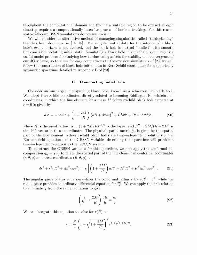
29

throughout the computational domain and finding a suitable region to be excised at eachtimestep requires a computationally intensive process of horizon tracking. For this reasonstate-of-the-art BSSN simulations do not use excision.

We will consider an alternative method of managing singularities called “turduckening”that has been developed in [14, 15]. The singular initial data for the interior of a blackhole’s event horizon is not evolved, and the black hole is instead “stuffed” with smoothbut constraint violating initial data. Simulating a black hole in spherically symmetry is auseful model problem for studying how turduckening affects the stability and convergence ofour dG scheme, so to allow for easy comparisons to the excision simulations of [23] we willfollow the construction of black hole initial data in Kerr-Schild coordinates for a sphericallysymmetric spacetime detailed in Appendix B of [23].

B. Constructing Initial Data

Consider an uncharged, nonspinning black hole, known as a schwarzschild black hole.We adopt Kerr-Schild coordinates, directly related to incoming Eddington-Finkelstein nullcoordinates, in which the line element for a mass M Schwarzschild black hole centered atr = 0 is given by

ds2 = −α2dt2 +

(1 +

2M

R

)(dR + βRdt

)2+R2dθ2 +R2 sin2 θdφ2, (90)

where R is the areal radius, α = (1 + 2M/R)−1/2 is the lapse, and βR = 2M/(R + 2M) isthe shift vector in these coordinates. The physical spatial metric gij is given by the spatialpart of the line element. schwarzschild black holes are time-independent solutions of theEinstein field equations, so the GBSSN variables describing this spacetime will provide atime-independent solution to the GBSSN system.

To construct the GBSSN variables for this spacetime, we first apply the conformal de-composition gij = χgij to relate the spatial part of the line element in conformal coordinates(r, θ, φ) and areal coordinates (R, θ, φ) as

dr2 + r2(dθ2 + sin2 θdφ2) = χ

[(1 +

2M

R

)dR2 +R2dθ2 +R2 sin2 θdφ2

]. (91)

The angular piece of this equation defines the conformal radius r by χR2 = r2, while theradial piece provides an ordinary differential equation for dR

dr. We can apply the first relation

to eliminate χ from the radial equation to give(√1 +

2M

R

)dR

R=dr

r. (92)

We can integrate this equation to solve for r(R) as

r =R

4

(1 +

√1 +

2M

R

)2

e2−2√

1+2M/R. (93)

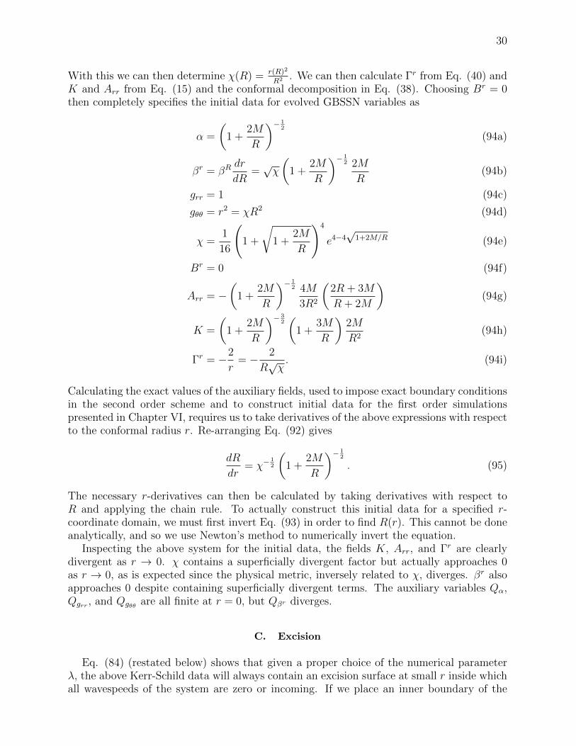
30

With this we can then determine χ(R) = r(R)2

R2 . We can then calculate Γr from Eq. (40) andK and Arr from Eq. (15) and the conformal decomposition in Eq. (38). Choosing Br = 0then completely specifies the initial data for evolved GBSSN variables as

α =

(1 +

2M

R

)− 12

(94a)

βr = βRdr

dR=√χ

(1 +

2M

R

)− 12 2M

R(94b)

grr = 1 (94c)

gθθ = r2 = χR2 (94d)

χ =1

16

(1 +

√1 +

2M

R

)4

e4−4√

1+2M/R (94e)

Br = 0 (94f)

Arr = −(

1 +2M

R

)− 12 4M

3R2

(2R + 3M

R + 2M

)(94g)

K =

(1 +

2M

R

)− 32(

1 +3M

R

)2M

R2(94h)

Γr = −2

r= − 2

R√χ. (94i)

Calculating the exact values of the auxiliary fields, used to impose exact boundary conditionsin the second order scheme and to construct initial data for the first order simulationspresented in Chapter VI, requires us to take derivatives of the above expressions with respectto the conformal radius r. Re-arranging Eq. (92) gives

dR

dr= χ−

12

(1 +

2M

R

)− 12

. (95)

The necessary r-derivatives can then be calculated by taking derivatives with respect toR and applying the chain rule. To actually construct this initial data for a specified r-coordinate domain, we must first invert Eq. (93) in order to find R(r). This cannot be doneanalytically, and so we use Newton’s method to numerically invert the equation.

Inspecting the above system for the initial data, the fields K, Arr, and Γr are clearlydivergent as r → 0. χ contains a superficially divergent factor but actually approaches 0as r → 0, as is expected since the physical metric, inversely related to χ, diverges. βr alsoapproaches 0 despite containing superficially divergent terms. The auxiliary variables Qα,Qgrr , and Qgθθ are all finite at r = 0, but Qβr diverges.

C. Excision

Eq. (84) (restated below) shows that given a proper choice of the numerical parameterλ, the above Kerr-Schild data will always contain an excision surface at small r inside whichall wavespeeds of the system are zero or incoming. If we place an inner boundary of the

31

computational domain within this excision surface, Sommerfeld boundary conditions reduceto taking the exterior solution equal to the interior solution and on physical grounds noboundary conditions need be imposed. We can therefore freely change our singular domainΩ = [0, rmax] to the domain [rmin, rmax] with the singularity excised so long as rmin < rexcision,defined to be the largest r satisfying Eq. (84), restated here:

βr ≥ max

(√2αχ

grr, α

√χ

grr,

√λ

grr

). (96)

D. Turduckening

The turduckening technique replaces singular black hole data with smooth but constraintviolating data. Many choices for this smooth stuffing data are possible, and since the exteriorsolution is causally disconnected from the turduckened solution in the interior of the horizonthe details of the stuffing are unimportant so long as the resulting simulations are stableand robust. Our choices are therefore strongly guided by numerical considerations.

We choose a region [0, rt] to be turduckened and make the replacement r → r in theequations for the initial data, where the stuffing transformation function r(r) is constructedto satisfy the conditions

r(0) = r0, r(rt) = rt, r = r for r > rt. (97)

We will further specify that the stuffing transformation r(r) has Ntur− 1 continuous deriva-tives at r(rt). If we choose r(r) to be a polynomial in r inside the turduckened region, thisprovides a system of Ntur + 1 linear equations that can be solved for the coefficients of thepolynomial.

In effect we are stretching the physically correct (non-singular) data for the region [r0, rt]over the whole turduckened region [0, rt]. Initial data turduckened in this manner willnaturally be constraint violating on [0, rt]. If the constraints H, M, and G evolve withwavespeeds that are not superluminal, these violations will not propagate to the outsideof the black hole’s event horizon. While this is not true in general for BSSN-type systems,evolution equations for the GBSSN constraint system as we have defined it can be calculatedand shown to have no superluminal wavespeeds [13], and so we may safely stuff the blackhole so long as rt lies within the event horizon. Despite this result, which formally holds inthe limit of the continuum and is rigorously discussed in [14], at finite resolution a numericalscheme may couple the interior and exterior solutions.

As an example of constructing the stuffing transformation r(r), consider Ntur = 4, forwhich r is rigged to satisfy r(r0) = r0, r(rt) = rt, r

′(rt) = 1, r′′(rt) = 0, and r′′′(rt) = 0.This provides a set of linear equations to be solved for the coefficients of the polynomialC1 + C2r

2 + C3r3 + C4r

4 + C5r5. This particular choice reproduces the polynomial used

as turducken stuffing in Eq. (37) of [14]. Note that there is no linear term included inthis polynomial. The turduckening procedure can introduce numerical instabilities if thegradient of the transformation is too steep. In this case removing the linear term produces amonotonic polynomial with smaller gradients than the corresponding 4th degree polynomialwith r0 = 0.1, rt = 0.4. The polynomials used in the numerical simulations described inSection V use r5 as the lowest order (non-constant) term to provide a transformation withshallow gradients for Ntur ≤ 8 on the above region.

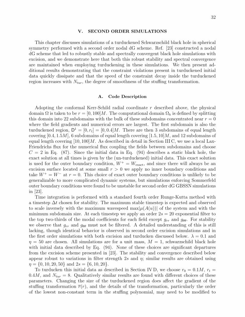
32

V. SECOND ORDER SIMULATIONS

This chapter discusses simulations of a turduckened Schwarzschild black hole in sphericalsymmetry performed with a second order nodal dG scheme. Ref. [23] constructed a nodaldG scheme that led to robustly stable and spectrally convergent black hole simulations withexcision, and we demonstrate here that both this robust stability and spectral convergenceare maintained when employing turduckening in these simulations. We then present ad-ditional results demonstrating that the constraint violations present in turduckened initialdata quickly dissipate and that the speed of the constraint decay inside the turduckenedregion increases with Ntur, the degree of smoothness of the stuffing transformation.

A. Code Description

Adopting the conformal Kerr-Schild radial coordinate r described above, the physicaldomain Ω is taken to be r = [0, 100]M . The computational domain Ωh is defined by splittingthis domain into 22 subdomains with the bulk of these subdomains concentrated near r = 0where the field gradients and numerical errors are largest. The first subdomain is also theturduckened region, D1 = [0, rt] = [0, 0.4]M . There are then 3 subdomains of equal lengthcovering [0.4, 1.5M ], 6 subdomains of equal length covering [1.5, 10]M , and 12 subdomains ofequal length covering [10, 100]M . As described in detail in Section III C, we use a local Lax-Friendrichs flux for the numerical flux coupling the fields between subdomains and chooseC = 2 in Eq. (87). Since the initial data in Eq. (94) describes a static black hole, theexact solution at all times is given by the (un-turduckened) initial data. This exact solutionis used for the outer boundary condition, W+ = Wexact, and since there will always be anexcision surface located at some small r > 0 we apply no inner boundary conditions andtake W+ = W− at r = 0. This choice of exact outer boundary conditions is unlikely to begeneralizable to more complicated dynamic systems, but simulations enforcing Sommerfeldouter boundary conditions were found to be unstable for second order dG GBSSN simulationsin [23].

Time integration is performed with a standard fourth order Runge-Kutta method witha timestep ∆t chosen for stability. The maximum stable timestep is expected and observedto scale inversely with the maximum wavespeed max|µ(A(u))| of the system and with theminimum subdomain size. At each timestep we apply an order 2s = 20 exponential filter tothe top two-thirds of the modal coefficients for each field except grr and gθθ. For stabilitywe observe that grr and gθθ must not be filtered. A detailed understanding of this is stilllacking, though identical behavior is observed in second order excision simulations and inthe first order simulations with both excision and turducken discussed below. λ = 0.1 andη = 50 are chosen. All simulations are for a unit mass, M = 1, schwarzschild black holewith initial data described by Eq. (94). None of these choices are significant departuresfrom the excision scheme presented in [23]. The stability and convergence described belowappear robust to variations in filter strength 2s and η; similar results are obtained usingη = 0, 10, 20, 50 and 2s = 6, 10, 20.

To turducken this initial data as described in Section IV D, we choose r0 = 0.1M , rt =0.4M , and Ntur = 8. Qualitatively similar results are found with different choices of theseparameters. Changing the size of the turduckened region does affect the gradient of thestuffing transformation r(r), and the details of the transformation, particularly the orderof the lowest non-constant term in the stuffing polynomial, may need to be modified to

33

account for this and ensure stability for different choices of r0 and rt. Varying Ntur has avery slight effect on the numerical value of the constraints at late times and a strong effecton the early-time behavior of the constraint violations, as described in detail below. In thesimulations described here, rt is chosen to lie on the boundary of a subdomain, but thereare no qualitative differences observed in simulations where this is not the case.

B. Long-term Stability and Convergence

FIG. 3. Stability and spectral convergence of the Hamiltonian constraint. The left plot shows the

L2 norm ||H||Ωh as a function of time for simulations with a range of different N . The right plot

shows a log scale of the L2 norm ||H||Ωh as measured at t = 10, 000 in these same six simulations

as a function of polynomial order N . For N=10, 12, 14, 16, 18, 20 the timesteps are respectively

∆t ≈ 0.0043, 0.003, 0.0023, 0.0017, 0.0014, 0.0011.

The first properties we look to verify for the scheme are stability and accuracy. Binaryblack hole simulations must run for long times and so the long-term stability of our modelsimulations is essential. The turduckened simulations in this section can be run to timet = 10, 000M with no growth in numerical error appearing. One of the most importantbenefits of a dG scheme is its spectral convergence, so it is especially important that weverify that the numerical error in our simulations does decrease exponentially when weincrease N , the order of the interpolating polynomials used to approximate the evolvedfields. This has been shown to hold for second order GBSSN simulations using excision in[23], and so our first major result is to show that these turduckened simulations still possessspectral convergence.

The main tool for monitoring the accuracy of our simulations is checking that the Hamil-tonian, momentum, and conformal connection constraints given in Eq. (45) hold at alltimes. We observe that the Hamiltonian constraint is the first to diverge when numericalinstabilities begin to develop, and so monitoring H provides a measure of the overall accu-racy of the simulation that is sensitive to numerical instabilities. The errors in the fieldsthemselves have been observed to share the same convergence properties as those shown forthe Hamiltonian constraint, that is we observe that for example ||(grr)num−(grr)analytic|| → 0so long as ||H|| → 0. Furthermore, since the constraint violations inside the turduckenedregion quickly shrink, as is discussed below, there is no significant difference between the

34

FIG. 4. Rapid decay in the Hamiltonian constraint at early times. This plot shows a log-scale of

the L2 norm ||H||Ωh as a function of log-scale time for a range of polynomial degrees N .

L2 norm over the entire domain and the norm taken with the turduckened region excluded,and so we simply monitor ||H||Ωh .

The long-term stability and spectral convergence of our turduckened dG scheme are shownin Fig. 3. As with second order excision simulations, there is no observed growth in ||H||Ωhover long times and the constraint violations measured at late times decrease exponentiallywith N . The magnitude of ||H||Ωh for a given value of N shown is orders of magnitudelarger than the corresponding value measured in the excision simulations of [23], but therate of convergence appears qualitatively similar to the excision case. At high resolutionsthere are no significant differences in the value of ||H||Ωh throughout the domain betweenturduckened and excision simulations after very early times. With N = 40 for example, theL2 norm ||H||Ωh is actually almost 25% lower at t = 10M in turduckened simulations then inexcision simulations with the same timestep and numerical parameters and an r-coordinatedomain of [0.4, 100]M with a subdomain structure identical to that described above for thisregion.

C. Further Results on Turduckening

1. Constraint Propagation

Since the turduckened fields in the initial data do not satisfy the constraints, ||H||Ωh istypically of order 1 at t = 0 and independent of N . This resolution independence is reason-able, as the constraint violations in the rest of the domain are orders of magnitude smallerthan the violations due to the turduckening at all resolutions considered, and so the overallL2 norm will depend only on the size of the turduckened region relative to the full domain.It is observed in turduckened finite difference simulations that these initial constraint vi-olations quickly dissipate, and by time t = 10M the interior solution has settled into anon-singular steady-state solution that satisfies the GBSSN constraints up to violations of

35

FIG. 5. Early time behavior of the Hamiltonian constraint inside the turduckened region with

various choices of Ntur. This plot shows the L2 norm ||H||D1 for the Hamiltonian constraint in

the turduckened region 0 ≤ r ≤ rt = 0.4M for times up to t = 5M . Each line corresponds to a

different degree of smoothness Ntur of the turduckened data at rt, where Ntur = 1 corresponds to

continuous data, Ntur = 2 corresponds to a continuous first derivative r′(r), etc. All simulations

shown in this plot are for N = 12.

the same order of magnitude as the exterior solution [14]. The mechanism proposed for thisin [14] is that the constraint violations propagate causally but the radial coordinate itself hasa superluminal velocity and so the coordinate region of constraint violation rapidly shrinks.Similar dissipation is observed in our simulations, and at high resolution the value of theconstraint violations even at the r = 0 grid point drops to the same order of magnitude asthe constraint violations throughout the rest of the domain by t = 4M . Fig. 4 demonstratesthis rapid decay in ||H|| averaged throughout the whole domain at early times as well aslate-time stability and convergence.

2. Dependence on Smoothness of Initial Data

The early-time decay of ||H||D1 , the L2 norm of the Hamiltonian constraint inside theturduckened region, is observed to depend on Ntur, the degree of smoothness of the stuffingtransformation r(r) at the interface rt. This is demonstrated in Fig. 5, which shows the earlytimes of simulations with N = 12 and various Ntur. So long as the stuffing transformationis at least differentiable (Ntur = 2) the constraint violations do quickly decay inside theturduckened region, with higher values of Ntur corresponding to faster decay. There is aslight but non-zero difference in the steady-state value of the constraint violations reachedinside the turduckened region, but this effect is not significant and has no clear relationshipto Ntur.

VI. FIRST ORDER SIMULATIONS

In this chapter we present a first order reduction of the GBSSN system we will refer to asFOBSSN and perform simulations of a black hole in spherical symmetry using the FOBSSN

36

system. We find that FOBSSN simulations using excision are stable and spectrally accuratewhen using exact boundary conditions, and unlike second order GBSSN simulations arestable and spectrally accurate with Sommerfeld outer boundary conditions. We have beenunable to achieve robustly stable FOBSSN simulations using turduckening. All simulationresults in this chapter were previously published in [11], but the surrounding discussion hasbeen heavily modified to follow the notation and scope of this thesis and in particular this isthe first explicit appearance of the evolution equations for the GBSSN auxiliary variables.

A. Auxiliary Variables and Constraints

To perform the first order reduction we promote the auxiliary fields to be evolved variablesrather than local variables calculated at each timestep. The necessary axillary fields for oursimulations in spherical symmetry are

Qα ≡ ∂rα, Qβr ≡ ∂rβr, Qχ ≡ ∂rχ, Qgrr ≡ ∂rgrr, Qgθθ ≡ ∂rgθθ. (98)

Note that the number of axillary variables that must be defined is greatly increased whenworking in full three-dimensional Cartesian coordinates. The definitions of the axillary fieldsintroduce new associated constraints for the FOBSSN system:

Ar ≡ Qα − ∂rα = 0 (99a)

Brr ≡ Qβr − βr = 0 (99b)

Cr ≡ Qχ − ∂rχ (99c)

Drrr ≡ Qgrr − ∂rgrr (99d)

Dθθr ≡ Qgθθ − ∂rgθθ. (99e)

The presence of these auxiliary constraints presents a genuine difference between theGBSSN and FOBSSN systems that is especially relevant to the construction of a tur-duckened FOBSSN scheme. In particular, recall that in the second order scheme theseconstraints define residuals used to enforce Galerkin conditions that define the auxiliaryvariables at each timestep. With FOBSSN the auxiliary variables are calculated accordingto their own discretized evolution equations (also recall we use a local Lax-Friendrichs fluxfor f ∗Q instead of the penalized central flux used in the second order scheme), so theseconstraints are no longer explicitly enforced in the numerical scheme.

The GBSSN system is trivially modified to be in the proper form for FOBSSN evolutionand constraint equations by replacing u′ → Q and u′′ → Q′. The evolution equations forthe auxiliary variables can be found simply by taking a spatial derivative of the evolutionequations for the corresponding field and using the commutativity of mixed partials and are

37

given by

∂tQα =QβrQα + βrQ′α − 2QαK − 2αK ′ − καAr (100a)

∂tQβr =Q2βr + βrQ′βr +

3

4Br′ − κβBrr (100b)

∂tQχ =QβrQχ + βrQ′χ +2

3K ′αχ+

2

3KQαχ+

2

3KαQχ −

QβrQgrrχ

3grr−βrQg′rrχ

3grr(100c)

− βrQgrrQχ

3grr+βrQ2

grrχ

3g2rr

− 2

3Q′βrχ−

2

3QβrQχ − κχCr

∂tQgrr =2

3QβrQgrr +

2

3βrQ′grr +

4

3QgrrQβr +

4

3grrQ

′βr − 2A′rrα− 2ArrQα (100d)

− 2QgrrβrQgθθ

3gθθ− 2grrQβrQgθθ

3gθθ−

2grrβrQ′gθθ

3gθθ+

2grrβrQ2

gθθ

3g2θθ

− κgDrrr

∂tQgθθ =1

3QβrQgrr +

1

3βrQ′gθθ +

A′rrgθθα

grr+ArrQgθθα

grr+ArrgθθQα

grr− ArrgθθαQgrr

g2rr

(100e)

− QgθθβrQgrr

3grr− gθθQβrQgrr

3grr−gθθβ

rQ′grr3grr

+gθθβ

rQ2grr

3g2rr

− 2

3QgθθQβr

− 2

3gθθQβr − κgDθθr.

Note that we have also introduced terms proportional to the auxillary constraints in eachevolution equation. These are trivially zero in the continuum limit and so can be addedfreely. The parameters κα, κβ, κχ and κg are chosen for numerical stability and allowfor damping of the axillary constraints. Evolution equations for the auxiliary constraints,found by taking the time derivative of Eq. (99), are given by simply replacing each auxiliaryvariable in Eq. (100) with the corresponding constraint. These equations for the evolution ofeach constraint therefore feature the corresponding damping parameter κ in each equation,and so setting these damping parameters to a sufficiently large value will indeed damp theauxiliary constraints.

B. Excision Results

To isolate the effects of turduckening from those of using the first order scheme moregenerally, we first consider dG simulations of the FOBSSN system using excision. The com-putational domain is taken to be r = [0.4, 50]M and for simplicity is divided into 100 equallyspaced subdomains. We use a local Lax-Friendrichs flux for all evolved fields, including theauxiliary variables, and as before choose C = 2, λ = 0.1, and η = 50 and take a unit mass,M = 1, schwarzschild black hole constructed in Kerr-Schild coordinates according to Eq.(94) as initial data. We apply an exponential filter of strength 2s = 20 to all fields exceptgrr and gθθ, including the auxiliary variables, and choose the timestep ∆t for stability. Theauxiliary damping parameters are chosen as κα = κβ = κχ = κg = 20.

Using exact outer boundary condition allows for long-term stable simulations with spec-tral convergence of the constraints, as with the second order scheme. In contrast with thesecond order scheme, enforcing Sommerfeld outer boundary conditions also allows for stableFOBSSN simulations. Fig. 6 demonstrates the long-term stability and spectral convergenceof the FOBSSN scheme with Sommerfeld boundary conditions. In an attempt to remove the

38

0 1000 2000 3000

10−7

10−5

10−3

10−1

‖H‖L

2

time (M)

N = 10N = 12N = 14N = 16N = 18N = 20

10 12 14 16 18 2010

−7

10−5

10−3

10−1

N

‖H‖ at T = 3,000M

FIG. 6. Stability and convergence of the Hamiltonian constraint with Sommerfeld boundary con-

ditions. The left plot shows the L2 norm ||H||Ωh as a log-scale function of time for simulations

run to t = 3, 000M at varying resolutions. The right plot shows log-scale ||H||Ωh as measured

at t = 3, 000M in these same simulations as a function of N . The highest two resolutions have

essentially reached double precision roundoff errors.

slow growth of the Hamiltonian constraint in time visible in this figure, we varied our nu-merical setup including the exponential filter parameters (the number of filtered modes, thedissipation exponent, and which variables to filter), the timestep, the Br damping parame-ter η, the numerical flux dissipation parameter, and the auxiliary field damping parameterswithout significant improvements.

C. Turduckening Results

As described in Chapter V, turduckening was straightforwardly incorporated into thesecond order GBSSN scheme and allowed for robustly stable simulations with no need forfine-tuning the numerical setup. This is not the case with the FOBSSN system. Thedefinition of the auxiliary fields creates an ambiguity in how to turducken to FOBSSNinitial data, since for example Qα(r) 6= ∂rα(r). This creates two distinct natural choicesfor defining turduckened auxiliary variables: 1-take the derivatives of the u sector variablesanalytically and compute their values at the turduckened grid points to calculate Qα(r) or2-apply the numerical derivative operator to the turduckened u sector variables to calculate∂rα(r). With the first choice the auxiliary constraints are violated in the initial data, whilewith the second choice the auxiliary constraints are satisfied but the turduckened initial datano longer represents the physically correct data for [r0, rt] stretched over the region [0, rt].We experimented with both choices and found that the region of constraint violations nolonger shrinks when using the first choice of data that violates the auxiliary constraints.A comparison in the constraint behavior of the system with both choices at early times isshown in Fig. 7.

We have been unable to achieve long-term stable turduckened simulations using eitherchoice. A typical evolution with either choice lasts on the order of tens of M to hundreds of

39

0 0.5 1 1.5 2 2.5 3 3.5

10−13

10−9

10−5

10−1

‖H‖ at T =0M

Auxiliary constraints satisfied.

Auxiliary constraints violated.

0 0.5 1 1.5 2 2.5 3 3.5

10−13

10−9

10−5

10−1

‖H‖ at T =1M

Auxiliary constraints satisfied.

Auxiliary constraints violated.

r(M)

FIG. 7. Snapshots of the Hamiltonian constraint for turduckened FOBSSN data which satisfies

(black line) and violates (dashed green line) the auxiliary constraints given in Eq. (99). The top

plot shows the L2 norm ||H||Ωh at t = 0 and the bottom plot shows this same norm at t = 1M .

Notice that only in the case where the auxiliary constraints are satisfied by the turduckened fields

does the region of constraint violation shrink during this time. The solid vertical line marks the

location of the event horizon, and the dashed line marks the location of the excision surface. The

large red asterisks on the horizontal axis mark the location of each subdomain boundary. The

turduckened region is specified by r0 = 0.1M and rt = 0.3M , also the boundary of the first

subdomain.

M , though some simulations with finely tuned choices of numerical parameters can last intothe thousands of M at lower resolution. Stability is not observed to increase with increasingresolution. Though the second choice of turduckened data that satisfies the auxiliary con-straints uniquely leads to a decay of the Hamiltonian constraint in the turduckened region,neither choice provides a clear advantage over the other in long-term stability.

VII. SCALAR FIELD SIMULATIONS

The simulations presented so far have all been limited to evolving vacuum spacetimes. Inthis chapter we consider coupling a simple and extensively studied matter system, namelya massless scalar field, to the GBSSN system and perform some basic simulations to verifythat dG methods can be used to straightforwardly construct a stable scheme for solving the

40

coupled system. After giving a brief introduction to the problem of simulating strongly grav-itating matter systems in Section A, we derive the necessary constructions for incorporatinga massless scalar field into our GBSSN simulations: evolution equations for the scalar fieldwith gravitational contributions written in terms of the GBSSN variables, the GBSSN mat-ter source terms for the scalar field, characteristics and boundary conditions for the mattersystem, and initial data for the scalar field. Section C presents some preliminary simulationresults: the matter system is robustly stable and spectrally accurate when evolved in flatspace and fully coupled simulations of a scalar pulse falling into a Kerr-Schild black hole arerobustly stable and result in radiation scattering off the black hole whose amplitude decaysas a power law in late times.

A. Overview

There are many strongly gravitating systems worth studying other than black holes. Evenwithin the context of gravitational wave detection, there are efforts underway to study thegravitational radiation emitted from the merger of two neutron stars through numericalsimulations [42]. In order to perform simulations of neutron stars, core-collapse supernovae,accretion flows, or other systems interesting to high-energy astrophysics or gravitationalwave astronomy we must solve the equations of GR in the presence of matter described bya non-zero stress-energy tensor.

Solving BSSN or other GR formulations in the presence of matter is often complicatedby the presence of shocks in the solution. Spectral methods are generally very sensitive tothe presence of shocks, and even state-of-the-art codes for spectral gravity evolution use aseparate finite-difference grid for evolving matter fields in neutron star simulations [34, 42].DG methods are an exception to this rule and are particularly well-suited to sharply resolvingshocks in solutions while maintaining spectral accuracy in evolving smooth pieces of thesolution. An example of this ability to manage shocks in the context of relativity is givenby [43], in which a dG scheme for general relativistic hydrodynamics is constructed and aone-dimensional model code is shown to robustly pass several tests of its capabilities forstably evolving shocks.

To the best of our knowledge, there have been no simulations constructed that evolve aBSSN-type system in the presence of matter fields using dG methods. In this chapter wewill present simulations of a very simple matter system: a massless scalar field in a spher-ically symmetric spacetime. With these simulations we look to demonstrate that our dGscheme can straightforwardly evolve a system with a dynamic matter field coupled to theGBSSN system without requiring the introduction of any new numerical tricks to achieverobust stability. Massless scalar fields have been studied extensively in other numerical sim-ulations, especially in the context of gravitational collapse, see [26] for a review and [24] forsimulations using the GBSSN system, and infall into a black hole. Gravitational collapse isdifficult to model in spherical coordinates since before the collapse there is no inner excisionsurface and suitable boundary conditions must be enforced at the inner boundary. Success-ful gravitational collapse simulations required imposing additional regularity conditions atthe origin [39] and sometimes employ at least one null coordinate instead of the sphericalcoordinates used here [16, 19]. Since the difficulty of finding proper conditions for stabilityat the origin is not present in three-dimensional Cartesian coordinate simulations and isa feature of using spherical coordinates rather than a general feature of evolving mattersystems, we will avoid this difficulty and limit ourselves to the study of systems possessing

41

an inner excision surface at all times.A simple scenario possessing such an excision surface is the infall of a localized pulse of

scalar field matter into a black hole. For simplicity we will employ the Kerr-Schild initialdata used in our previous simulations and limit ourselves sufficiently small pulses whosegravitational effects can be treated as perturbations of this black hole spacetime ratherthan undertake the construction of initial data that satisfies the GBSSN constraints for ablack hole in the presence of matter. This simple scenario still possesses interesting physics,and numerous simulations of black holes perturbed by scalar fields show that in generalcircumstances as the black hole relaxes from a perturbed state back to its stationary (“nohair”) state it emits scalar radiation whose amplitude decays as a power-law at late timesas it scatters off spacetime curvature [2, 5, 6, 30].

B. Scheme for Simulating a Massless Scalar Field

1. First Order Evolution Equations

Throughout this chapter we will consider a scalar field ϕ(t, x) that satisfies the masslessKlein-Gordon equation (the source-free covariant wave equation):

ϕ ≡ ∇µ∇µϕ = 0 (101)

To find the gravitational coupling of this field in terms of our evolved GBSSN variables, wecan use the fact that

√−g 5 is a scalar density of weight +1 and an identity ∇µ

√−g =

0 derived from metric compatibility [20] to derive a useful identity for the Klein-Gordonequation:

ϕ = 1√−g∇µ (

√−g∂µϕ) = 1√

−g∂µ (√−g∂µϕ) (102)

= 1√−g∂µ (

√−g gµν∂νϕ) .

Using this form of the Klein-Gordon equation and our definitions for the metric componentsin Eq. 7 6, we can express the Klein-Gordon equation for ϕ as√−gϕ = ∂t

(√−g gtt∂tϕ+

√−g gtr∂rϕ

)+ ∂r

(√−g gtr∂tϕ+

√−g grr∂rϕ

)(103)

= ∂t

[α−2√−g (−∂tϕ+ βr∂rϕ)

]+ ∂r

[α−2√−gβr (∂tϕ− βr∂rϕ) +

√−g γrr∂rϕ

].

The determinant of the physical metric is simply related to the determinant of the spatialmetric by g = −α2γ. This allows us to express

√−g in terms of our evolved GBSSN variables

as √−g = α

√γ = αχ−3/2√g = αχ−3/2√grrgθθ sin θ. (104)

5 Remember that gµν is the physical spacetime metric, γµν is the spatial piece of the physical metric, and

the notation gµν is reserved for the conformal spatial metric defined by gµν ≡ χγµν .6 In the spherically symmetric reduction we have in particular gtt = −α−2, gtr = α−2βr, and grr =

γrr − α−2(βr)2

42

To recast Eq. (103) as a first order PDE, as is commonly done in simulations of scalar fieldsin numerical relativity [29], we introduce the following variables:

Φ ≡ ∂rϕ (105a)

Π ≡ α−2√−g(∂tϕ− βr∂rϕ)(sin θ)−1 =

√grrgθθ

αχ3/2(∂tϕ− βr∂rϕ). (105b)

Remembering that the normal vector for our foliation of spacelike hypersurfaces in ChapterII is given by nµ = α−1(1,−βi), Π is actually just the derivative normal to the spacelikehypersurfaces weighted by

√−g. We will use Φ and Π as the evolved variables for simulations

of the scalar field ϕ. Their evolution equations are found by applying commutativity of mixedpartials (∂tΦ = ∂r∂tϕ) and Eq. (103):

∂tϕ = βrΦ +αχ3/2

√grrgθθ

Π (106a)

∂tΦ = ∂r

(βrΦ +

αχ3/2

√grrgθθ

Π

)(106b)

∂tΠ = ∂r

(αgθθ√χgrr

Φ + βrΠ

). (106c)

2. Stress-Energy Tensor and Source Terms

The above equations allow us to evolve the scalar field in the presence of a curved space-time background. To fully describe the system we must also determine how coupling thescalar field ϕ to that spacetime background affects the geometry. The GBSSN system pre-sented in Eqs. (44), (45) is valid for a spacetime with an arbitrary collection of matterdescribed by a stress-energy tensor T µν . Describing the response of the GBSSN variablesto the scalar field therefore amounts to determining the stress-energy tensor for ϕ and inparticular the matter variables ρ, S, STFrr , and jr defined at the end of Section II C that arefeatured in the GBSSN system.

The Lagrangian for our scalar field is given by LM = −12∇µϕ∇µϕ, as may be verified by

varying the action

SM =

∫d4x LM =

∫d4x

[−1

2∇µϕ∇µϕ

]. (107)

After a few integrations by parts where we ignore boundary terms (we assume ϕ(±∞)→ 0)this variation gives δSM = (∇µ∇µϕ)δϕ = 0, and so the Klein-Gordon equation is recoveredas the equation of motion for ϕ. With the action in general relativity expressed in the form

S =

∫d4x

[1

16πGLG + LM

]√−g, (108)

the Einstein field equations are recovered by demanding that the variation δSδgµν

vanish. To

recover the non-vacuum Einstein field equations the stress-energy tensor must be related tothis action by Tµν = −2√

−gδLMδgµν

. Carrying out this variation even for the simple scalar field

Lagrangian is still a non-trivial calculation and we will not work it out explicitly. The resultis given by [18]

Tµν ≡−2√−g

δLMδgµν

= ∇µϕ∇νϕ−1

2gµνg

ρσ∇ρϕ∇σϕ. (109)

43

This can be expressed in terms of the GBSSN variables and the matter variables ϕ, Φ, andΠ as

Tµν = ∂µϕ∂νϕ−1

2gµν[α−2(−(∂tϕ)2 + 2βr∂tϕ− (βr∂rϕ)2) + γrr(∂rϕ)2

](110)

= ∂µϕ∂νϕ+1

2gµν

(− χ

grrΦ2 +

χ3

grrg2θθ

Π2

).

The matter variables ρ, S, STFrr , and jr appear as source terms in the GBSSN evolution

equations, and ρ and jr further specify the proper value of the Hamiltonian and momen-tum constraints are related to the components of the stress-energy tensor and the GBSSNvariables by

ρ ≡ nµnνTµν = α−2(Ttt − 2βrTtr + (βr)2Trr

)(111a)

S ≡ TrSij = TrTij =χ

grrTrr +

2χ

gθθTθθ (111b)

STFrr ≡ Trr −

1

3χSgrr (111c)

jr ≡ (−γrµnνTµν) =χ

αgrr(βrTrr − Ttr) (111d)

There is little insight gained from substituting Eq. (110) into Eq. (111) to express thesesource terms in terms of the evolved matter variables, and in the simulations to follow wesimply perform this substitution numerically.

3. Boundary Conditions

The evolution equation for ϕ features a zero principle part, and so we can specify f ∗ϕ =fϕ = 0 just as we specified f ∗u = fu = 0 when considering the abstract GBSSN system. Wetherefore do not need to apply any boundary conditions to ϕ. The evolution equations forΦ and Π feature zero source terms, and so Sommerfeld boundary conditions are a naturalchoice. These can be derived by considering the characteristic variables and wavespeedsof the evolution equations as in the construction sketched in Section III C. Since we arenow working with a far simpler system than the GBSSN equations we will perform theconstruction for the first order Klein-Gordon system in detail. We begin by writing theevolution system for Φ and Π as a matrix equation analogous to the abstract GBSSN systemin Eq. (79) as

∂t

(ΦΠ

)+B(u) ∂r

(ΦΠ

)≡ ∂t

(ΦΠ

)+

(−βr − αχ3/2

√grrgθθ

− αgθθ√χgrr

−βr

)∂r

(ΦΠ

)= 0. (112)

The matrix B(u) is diagonalizable with eigenvalues are given by

µ± = −βr ± α√

χ

grr. (113)

These define the wavespeeds of the matter evolution system. Note that they match thewavespeeds µ±5 of the GBSSN system given in Eq. (80). This simplifies the numerics of

44

scalar field simulations since adding the matter evolution equations to the GBSSN systemdoes not introduce any new distinct wavespeeds that could impact the existence or locationof an excision surface or force a change in our choice of stable timestep.

The corresponding eigenvectors of the matrix B(u) are given by(gθθ/χ

1

)and

( −gθθ/χ1

).

The matter evolution system can therefore be expressed as

∂t

(ΦΠ

)+

1

2

(gθθχ−gθθ

χ

1 1

)(µ− 00 µ+

)( χgθθ

1

− χgθθ

1

)∂r

(ΦΠ

)= 0. (114)

The characteristic fields are given by applying the matrix U ≡(

χgθθ

1

− χgθθ

1

)to our system

vector Y ≡ ( ΦΠ ) in order to transform the system into the eigenbasis of B(u). This provides

us with the incoming and outgoing solutions X− and X+7,(X−

X+

)≡ U

(ΦΠ

)=

( gθθχ

Φ + Π

−gθθχ

Φ + Π

). (115)

Remember that in a dG scheme coupling between subdomains occurs through the nu-merical flux and so boundary conditions are imposed by specifying the external solution Y +

to be used in calculated the numerical flux in the boundary subdomain. At the outermostsubdomain DK we wish to enforce a Sommerfeld boundary condition, that is the exter-nal solution Y +

K should have zero incoming characteristics and should match the outgoingcharacteristics of the numerical solution Y −K . The above relation between the characteristicvariables and the matter evolution system variables can be used to express this condition asa system of linear equations for the external fields Φ+

K and Π+K in terms of the internal fields

Φ−K and Π−K :

X−(Y +K ) =

gθθχ

Φ+K + Π+

K = 0 (116a)

X+(Y +K ) = −gθθ

χΦ+K + Π+

K = X+(Y −K ) = −gθθχ

Φ−K + Π−K . (116b)

As a brief aside, note that there is an apparent ambiguity in choosing the values of theGBSSN variables used to calculate X+(Y +

K ). This ambiguity is resolved by noting that onlythe variables in the u sector of the GBSSN system are present. Due to the presence ofthe auxiliary sector Q we take fu = f ∗u = 0 and apply no boundary conditions to the usector. This is equivalent to u+ = u− at the boundary, and so we can safely use u−, theGBSSN variables of the numerical solution, when calculating all the characteristic variablesX±(Y ±K ). A similar situation occurs when calculating Sommerfeld boundary conditions forthe GBSSN system since the matrix A(u) depends on this same sector. With this resolved,

7 Due to an unfortunate coincidence of notation it is standard to denote both incoming/outgoing solutions

and the interior/exterior solutions to a subdomain in dG with ±. The characteristic variables X+ and

X− will always denote the outgoing (traveling from small r to large r) and incoming (large to small r)

solution, while we reserve Y +k and Y −

k to denote the solution vector on the exterior and interior of the

k-the subdomain.

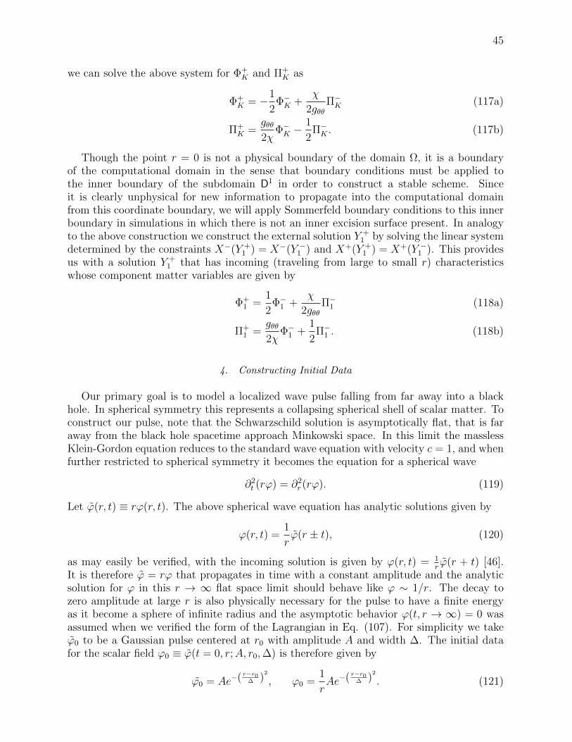
45

we can solve the above system for Φ+K and Π+

K as

Φ+K = −1

2Φ−K +

χ

2gθθΠ−K (117a)

Π+K =

gθθ2χ

Φ−K −1

2Π−K . (117b)

Though the point r = 0 is not a physical boundary of the domain Ω, it is a boundaryof the computational domain in the sense that boundary conditions must be applied tothe inner boundary of the subdomain D1 in order to construct a stable scheme. Sinceit is clearly unphysical for new information to propagate into the computational domainfrom this coordinate boundary, we will apply Sommerfeld boundary conditions to this innerboundary in simulations in which there is not an inner excision surface present. In analogyto the above construction we construct the external solution Y +

1 by solving the linear systemdetermined by the constraints X−(Y +

1 ) = X−(Y −1 ) and X+(Y +1 ) = X+(Y −1 ). This provides

us with a solution Y +1 that has incoming (traveling from large to small r) characteristics

whose component matter variables are given by

Φ+1 =

1

2Φ−1 +

χ

2gθθΠ−1 (118a)

Π+1 =

gθθ2χ

Φ−1 +1

2Π−1 . (118b)

4. Constructing Initial Data

Our primary goal is to model a localized wave pulse falling from far away into a blackhole. In spherical symmetry this represents a collapsing spherical shell of scalar matter. Toconstruct our pulse, note that the Schwarzschild solution is asymptotically flat, that is faraway from the black hole spacetime approach Minkowski space. In this limit the masslessKlein-Gordon equation reduces to the standard wave equation with velocity c = 1, and whenfurther restricted to spherical symmetry it becomes the equation for a spherical wave

∂2t (rϕ) = ∂2

r (rϕ). (119)

Let ϕ(r, t) ≡ rϕ(r, t). The above spherical wave equation has analytic solutions given by

ϕ(r, t) =1

rϕ(r ± t), (120)

as may easily be verified, with the incoming solution is given by ϕ(r, t) = 1rϕ(r + t) [46].

It is therefore ϕ = rϕ that propagates in time with a constant amplitude and the analyticsolution for ϕ in this r → ∞ flat space limit should behave like ϕ ∼ 1/r. The decay tozero amplitude at large r is also physically necessary for the pulse to have a finite energyas it become a sphere of infinite radius and the asymptotic behavior ϕ(t, r → ∞) = 0 wasassumed when we verified the form of the Lagrangian in Eq. (107). For simplicity we takeϕ0 to be a Gaussian pulse centered at r0 with amplitude A and width ∆. The initial datafor the scalar field ϕ0 ≡ ϕ(t = 0, r;A, r0,∆) is therefore given by

ϕ0 = Ae−( r−r0∆ )2

, ϕ0 =1

rAe−( r−r0∆ )

2

. (121)

46

From this we can immediately calculate Φ0 ≡ Φ(t = 0, r;A, r0,∆) from the definition Φ =∂rϕ and take

Φ0 =1

r∂rϕ0 −

1

r2ϕ0 =

2A(r0 − r)r∆2

e−( r−r0∆ )2

− A

r2e−( r−r0∆ )

2

. (122)

Since Π depends on ∂tϕ, our choice for Π0 ≡ Π(t = 0, r;A, r0,∆) will be used to enforce thatthe pulse is incoming. The incoming solution ϕ(r, t) = 1

rϕ(r + t) satisfies ∂tϕ = 1

r∂t(rϕ) =

1r∂r(rϕ), and so our initial data should satisfy ∂tϕ0 = Φ0 + 1

rϕ0. This allows us to specify

Π0 according to its definition, Eq. (105a), as

Π0 =

√grrgθθ

αχ3/2

(Φ0(1− βr) +

ϕ0

r

)(123)

To verify the accuracy of our dG scheme for solving the scalar field evolution equations,Eq. (106), we will consider simulations in Minkowski space, defined in spherical coordinatesby the metric ds2 = −dt2 + dr2 + r2dΩ2. This specifies initial data for the evolved GBSSNfields given by

grr = 1, gθθ = r2, χ = 1,

K = 0, Arr = 0, Γr = −2/r,

α = 1, βr = 0, Br = 0.

(124)

In particular we have for this initial geometry Π0 = r2Φ0 + rϕ0.The remainder of our simulations will use the Kerr-Schild initial data given in Eq. (94)

to model the infall of our scalar field pulse into an un-charged, non-rotating black hole. Notethat this choice of initial data actually violates the Hamiltonian and momentum GBSSNconstraints since the Kerr-Schild data satisfies the vacuum constraints but the presence ofthe scalar field pulse dictates ρ, jr 6= 0. We are therefore limited to situations in which thescalar field pulse can be considered as a perturbation of the black hole spacetime. As long asthe initial amplitude A and width ∆ are sufficiently small compared to the black hole massM , the initial constraint violations will likewise be small and there will be no significant lossof accuracy so long as the violations do not grow in time or lead to numerical instabilities.Since these are analytic constraint violations in the data rather than numerical artifacts wedo not expect them to shrink with increasing computational resolution and we will thereforenot be able to measure the convergence of the scheme by monitoring the magnitude of theGBSSN constraints.

C. Simulation Results

1. Accuracy in Minkowski Space

In order to directly verify the accuracy of our scheme for solving the matter evolutionequations, we begin by simulating the propagation of a wave pulse in Minkowski space andcomparing our numerical pulse to the known analytic solution. Since Γr still diverges atr = 0 (an artifact of using spherical coordinates), we place our inner boundary slightly awayfrom the origin and take our domain Ω to be r = [0.4, 300]. The computational domainΩh is defined by splitting this into 7 subdomains of equal length covering [0.4, 10] and 30

47

FIG. 8. Snapshots of the scalar pulse in Minkowski space and convergence. The left plot shows

snapshots of a pulse with A = 1, ∆ = 5, r0 = 200, and resolution N = 10 at various times.

The solid line shows the initial pulse at t = 0, and the dashed lines show the pulse at t =

20, 40, 60, 80, 100. The left plot demonstrates the convergence of the scheme and shows log-scale

||∆ϕ||Ωh ≡ ||ϕ− ϕexact||Ωhwith increasing N . These simulations used A = 1, ∆ = 3, and r0 = 150

and the norm is measured at t = 10.

subdomains of equal length covering [10, 300]. We use a local Lax-Friendrichs flux withC = 2 for the numerical fluxes f ∗Φ and f ∗Π and as described above take f ∗ϕ = 0. We usethe initial data for a purely incoming wave pulse given by Eqs. (121)-(123) and initializethe GBSSN variables to the Minkowski space values given in Eq. (124). Only the mattervariables are evolved; the GBSSN variables are left constant with these values. We applySommerfeld boundary conditions at the inner and outer boundaries as given by Eq. (118)and Eq. (117) respectively. As before we use a fourth-order Runge Kutta method for timeevolution with the timestep ∆t chosen for stability. Since the matter evolution equationsare linear there should be no aliasing error and we do not apply any filter to the system.

Simulations of this incoming wave pulse are robustly stable for all choices of A, ∆, andr0 we have considered. Since there is no length scale other than the size of the domain thereare no qualitative differences when A is varied over many orders of magnitude from 10−5 to105. The presence of boundaries is not observed to introduce any complications, and uponreaching the inner boundary the incoming pulse reflects back in a stable manner. We cancalculate the analytic solution ϕexact at later times according to ϕexact(r, t) = 1

rϕ0(t + r),

where ϕ = rϕ as described above. Calculating the L2 norm ||ϕ − ϕexact||Ωh provides adirect measurement of the accuracy of these simulations. Fig. 8 shows that this errordecays exponentially with increasing polynomial order N , so our scheme for solving thematter evolution equations possesses spectral convergence, as expected. Snapshots of ϕ(x)at intervals of t = 20 from t = 0 to t = 100 are also shown in Fig. 8 and demonstrate thatthe scalar field has the desired qualitative behavior of an incoming Gaussian pulse whosewidth stays constant and amplitude grows with decreasing r.

48

FIG. 9. Pulse amplitude during infall and power-law decay. The left plot shows max(|ϕ|) over the

domain Ω during the full infall simulation from t = 0 to t = 500. The black hole is unit mass,

M = 1, and the initial pulse has parameters A = 10−2M , ∆ = 3, and r0 = 100. The right plot

shows a log-log plot of max(|ϕ|) over the domain for late times t = 250 to t = 500. The straight

line in the log-log plot demonstrates a power-law decay.

2. Infall with a Kerr-Schild Black Hole

We now consider simulations with non-trivial gravitational coupling in which both thematter and GBSSN systems are evolved. We use the second order scheme to evolve thegravity sector and find that so long as the scalar field is small enough to be treated as aperturbation on the black hole spacetime no changes need to be make to the numericalsetup used in Chapter V: we take C = 2, λ = 0.1, and η = 50 and consider a Schwarzschildblack hole described in Kerr-Schild coordinates as before. To minimize any boundary effectswe use a large computational domain Ω of r = [0.4, 600]M . With this domain choice thesingularity of the black hole is managed through excision. The computational domain Ωh isdefined by splitting the region [0.4, 10]M into 7 subdomains of equal length and the region[10, 600]M into 60 subdomains of equal length. We use a local Lax-Friendrichs flux for allevolved fields, including the scalar field variables Φ and Π and take fϕ = 0 since Φ = ∂rϕdefines an auxiliary variable analogous to the Q sector of the abstract GBSSN system. Asbefore we apply an exponential filter of strength 2s = 20 to all fields except grr and gθθ,including the matter variables ϕ, Φ, and Π and choose the timestep ∆t for stability. Weuse exact outer boundary conditions for the GBSSN fields and the Sommerfeld boundaryconditions described above for Φ and Π.

Typical choices of initial data for the incoming pulse are A = 10−2M , ∆ = 3, andr0 = 100. This creates Hamiltonian constraint violations on the order of 10−8 near thepulse since the Kerr-Schild data satisfies the vacuum constraints. Constraint violations ofthis order propagate with the pulse and grow along with the amplitude as it moves inward,but there is no sign of uncontrolled growth in the constraints or changes in the qualitativeshape of the GBSSN fields. With an initial amplitude of A = 1M this is no longer the case:deformations of the metric are immediately visible and the constraint violations steadilygrow until an instability develops just after t = 100. For A = 10M an instability developsalmost immediately. This is consistent with the idea that we can only model the scalar field

49

as a perturbation of the black hole geometry, and as long as the amplitude is taken to besufficiently small relative to the black hole mass there is no sign of constraint growth orinstability in simulations lasting for times in the hundreds of M .

The maximum absolute value (L∞ norm) of the scalar field ϕ is shown as a function oftime in Fig. 9. Qualitatively, the amplitude of the pulse increases as it moves inward, asin Minkowski space, until it reaches the black hole. The amplitude then falls off rapidlyas it the pulse enters the horizon and travels off the inner boundary. After this initialinfall, scalar matter is observed to radiate outward from the black hole. At late times themagnitude of this radiation decays as a power-law, as shown in Fig. 9. The precise decayrate is observed to depend on the details of the initial pulse. Observations of outgoing scalarradiation with a late-time power law decay are consistent with other numerical and analyticresults, and in particular [30] calculates the precise exponent for the decay of each mode ofa spherical harmonic decomposition of a scalar waveform. A straightforward application ofthis simulation code would be to monitor the amplitude of the radiated field at a fixed (areal)radius and compare the decay rate to the values predicted for different pulses. A furtherimmediate application would be to consider more general initial pulses and study for examplethe absorption rates of different pulses as considered in finite difference simulations in [48].More generally we hope that dG methods will soon be applied to more complicated andastrophysically interesting matter systems than the simple scalar field we have consideredhere.

VIII. CONCLUSION

Discontinuous Galerkin methods appear to be a promising technique for simulations innumerical relativity. After presenting a review of reformulating GR for initial value prob-lems and the GBSSN system and a description of a dG scheme for solving the system andthe turduckening technique for managing singular initial data describing black holes, wepresented a number of new black hole simulations using dG methods that build upon thescheme constructed by Field et. al. in [23]. This previous work presented robustly stableand spectrally accurate second order dG simulations of a black hole in spherical symmetrythat removed the singularity from the computational grid via excision, and in this thesis weshowed that robust stability and spectral convergence were maintained when the interiorof the black hole was included in the domain but the singularity was smoothed away usingthe turduckening technique. We further found that the initial constraint violations due toturduckening quickly decayed, as observed in the turduckened finite difference simulations of[14], and moreover that the rate of this decay increased with the smoothness of the stuffingtransformation at the boundary of the turduckened region. At high resolution simulationsusing excision and turduckened were found to have similar levels of constraint violationsonce these violations in the initial data decayed.

We then presented a first order reduction of the GBSSN system and the results of dGsimulations of this FOBSSN system recently published in [11]. Unlike the second order simu-lations that relied on using an analytic solution for outer boundary conditions, dG FOBSSNsimulations were found to be stable and spectrally accurate with Sommerfeld boundaryconditions enforced at the outer boundary. We discovered an ambiguity in turduckeningthe auxiliary fields in FOBSSN initial data were unable to construct stable simulations ofFOBSSN using turduckening.

Finally, we considered dG simulations with dynamic matter fields coupled to the gravity

50

sector. For simplicity we considered the infall of a massless scalar field into a schwarzschildblack hole. We presented a derivation of evolution equations for this scalar field in terms ofour evolved GBSSN variables and constructed a spectrally accurate dG solver for the Klein-Gordon equation that we then incorporated into our second order black hole simulationswith the appropriate gravitational coupling. The resulting simulations were found to berobustly stable so long as the amplitude of the initial incoming Gaussian pulse had anamplitude sufficiently small relative to the black hole mass that its gravitational effectscould effectively be considered a perturbation on the black hole spacetime. We observedthat after this incoming pulse fell into the black hole outgoing scalar radiation was emittedthat at late times decayed according to a power-law.

It is our hope that this work can be expanded towards the construction of a general three-dimensional dG BSSN solver capable of efficiently simulating binary black hole collisions aswell as non-vacuum simulations containing dynamic matter fields.

IX. ACKNOWLEDGMENTS

I would like to firstly thank my adviser Jan Hesthaven for all his support. I also owea huge debt to Scott Field for his tireless help and email correspondence during and afterhis time at Brown. I would like to thank Stephen Lau for all his behind the scenes supporton building the dG code. I would also like to thank Manuel Tiglio for all his help with theFOBSSN paper along with and everyone else who contributed to the paper. I want to thankBrown University and the UTRA program for supporting me on this research in summer2011. Finally, I want to give a big thanks to all my friends and roommates who put up withme talking about turduckening for over a year now.

[1] Miguel Alcubierre, Bernd Bruegmann, Peter Diener, Michael Koppitz, Denis Pollney, et al.

Gauge conditions for long term numerical black hole evolutions without excision. Phys.Rev.,

D67:084023, 2003.

[2] Elspeth W. Allen, Elizabeth Buckmiller, Lior M. Burko, and Richard H. Price. Radiation tails

and boundary conditions for black hole evolutions. Phys.Rev., D70:044038, 2004.

[3] Douglas N. Arnold, Franco Brezzi, Bernardo Cockburn, and L. Donatella Marini. Unified

analysis of discontinuous galerkin methods for elliptic problems. SIAM J. Numer. Anal.,

39(5):1749–1779, 2001.

[4] Richard L. Arnowitt, Stanley Deser, and Charles W. Misner. The Dynamics of general rela-

tivity. 1962. Gravitation: an introduction to current research, Louis Witten ed. (Wilew 1962),

chapter 7, pp 227-265.

[5] Leor Barack. Late time dynamics of scalar perturbations outside black holes. 1. A Shell toy

model. Phys.Rev., D59:044016, 1999.

[6] Leor Barack. Late time dynamics of scalar perturbations outside black holes. 2. Schwarzschild

geometry. Phys.Rev., D59:044017, 1999.

[7] Thomas W. Baumgarte. Black Holes: from Speculations to Observations. AIP Conf.Proc.,

861:161–175, 2006.

[8] Thomas W. Baumgarte and Stuart L. Shapiro. On the numerical integration of Einstein’s

field equations. Phys.Rev., D59:024007, 1999.

51

[9] Thomas W. Baumgarte and Stuart L. Shapiro. Numerical relativity and compact binaries.

Phys.Rept., 376:41–131, 2003.

[10] J. David Brown. Covariant formulations of BSSN and the standard gauge. Phys.Rev.,

D79:104029, 2009.

[11] J. David Brown, Peter Diener, Scott E. Field, Jan S. Hesthaven, Frank Herrmann, et al.

Numerical simulations with a first order BSSN formulation of Einstein’s field equations. 2012.

[12] J.David Brown. Conformal invariance and the conformal-traceless decomposition of the grav-

itational field. Phys.Rev., D71:104011, 2005.

[13] J.David Brown. BSSN in spherical symmetry. Class.Quant.Grav., 25:205004, 2008.

[14] J.David Brown, Peter Diener, Olivier Sarbach, Erik Schnetter, and Manuel Tiglio. Turduck-

ening black holes: An Analytical and computational study. Phys.Rev., D79:044023, 2009.

[15] J.David Brown, Olivier Sarbach, Erik Schnetter, Manuel Tiglio, Peter Diener, et al. Excision

without excision: The Relativistic turducken. Phys.Rev., D76:081503, 2007.

[16] Lior M. Burko and Amos Ori. Late time evolution of nonlinear gravitational collapse.

Phys.Rev., D56:7820–7832, 1997.

[17] Gioel Calabrese, Jorge Pullin, Olivier Sarbach, and Manuel Tiglio. Convergence and stability

in numerical relativity. Phys.Rev., D66:041501, 2002.

[18] Sean M. Carroll. Spacetime and geometry: An introduction to general relativity. 2004.

[19] H.P. De Oliveira and I. Damiao Soares. Galerkin method in the gravitational collapse: A

Dynamical system approach. Phys.Rev., D65:064029, 2002.

[20] R. d’Inverno. Introducing Einstein’s relativity. 1992.

[21] Manfredo P. do Carmo. Riemannian Geometry. Birkhauser, Boston, MA, 1992.

[22] Scott E. Field. Applications of discontinuous galerkin methods to computational general

relativity. Brown University PhD Dissertation, 2011.

[23] Scott E. Field, Jan S. Hesthaven, Stephen R. Lau, and Abdul H. Mroue. Discontinuous

Galerkin method for the spherically reduced BSSN system with second-order operators. Phys.

Rev., D82:104051, 2010.

[24] J.A. Gonzalez and F.S. Guzman. Accretion of phantom scalar field into a black hole. Phys.Rev.,

D79:121501, 2009.

[25] Eric Gourgoulhon. 3+1 formalism and bases of numerical relativity. 2007. Lecture notes.

[26] Carsten Gundlach. Critical phenomena in gravitational collapse. Phys.Rept., 376:339–405,

2003.

[27] Carsten Gundlach and Jose M. Martin-Garcia. Symmetric hyperbolic form of systems of

second order evolution equations subject to constraints. Phys.Rev., D70:044031, 2004.

[28] Carsten Gundlach and Jose M. Martin-Garcia. Hyperbolicity of second-order in space systems

of evolution equations. Class.Quant.Grav., 23:S387–S404, 2006.

[29] Carsten Gundlach and Jose M. Martin-Garcia. Critical phenomena in gravitational collapse.

Living Rev.Rel., 10:5, 2007.

[30] Carsten Gundlach, Richard H. Price, and Jorge Pullin. Late time behavior of stellar collapse

and explosions: 1. Linearized perturbations. Phys.Rev., D49:883–889, 1994.

[31] J Hesthaven. Nodal high-order methods on unstructured grids i. time-domain solution of

maxwells equations. Journal of Computational Physics, 181(1):186–221, 2002.

[32] J. S. Hesthaven and T. Wasburton. Nodal Discontinuous Galerkin Methods Algorithms, Anal-

ysis, and Applications. Springer, 2007.

[33] Russell A. Hulse. The discovery of the binary pulsar. Rev. Mod. Phys., 66:699–710, Jul 1994.

52

[34] J. Kaplan, C. Ott, C. Muhlberger, M. Duez, F. Foucart, and M. Scheel. Simulations of

Neutron-Star Binaries using the Spectral Einstein Code (SpEC). In APS Meeting Abstracts,

page 14005, February 2010.

[35] Irving Kaplansky. Linear Algebra and Geometry: Second Course. Chelsea Pub Co, 1974.

[36] Paola Leaci. Searching for continuous gravitational wave signals using LIGO and Virgo de-

tectors. J.Phys.Conf.Ser., 354:012010, 2012.

[37] J. M. Lee. Riemannian Manifolds: An Introduction to Curvature. 1997.

[38] J.M. Lee. Introduction to Smooth Manifolds. 2005.

[39] R.L. Marsa and M.W. Choptuik. Black hole scalar field interactions in spherical symmetry.

Phys.Rev., D54:4929–4943, 1996.

[40] Charles W. Misner, K.S. Thorne, and J.A. Wheeler. Gravitation. 1974.

[41] Dario Nunez and Olivier Sarbach. Boundary conditions for the Baumgarte-Shapiro-Shibata-

Nakamura formulation of Einstein’s field equations. Phys.Rev., D81:044011, 2010.

[42] Harald P. Pfeiffer. Numerical simulations of compact object binaries. 2012.

[43] David Radice and Luciano Rezzolla. Discontinuous Galerkin methods for general-relativistic

hydrodynamics: formulation and application to spherically symmetric spacetimes. Phys.Rev.,

D84:024010, 2011.

[44] Bernard Schutz. Geometrical Methods of Mathematical Physics. 1980.

[45] Bernard F. Schutz. A First Course In General Relativity. Cambridge, Uk: Univ. Pr. ( 1985)

376p.

[46] W.A. Strauss. Partial Differential Equations: An Introduction. Wiley, 1992.

[47] Slava G. Turyshev. Experimental Tests of General Relativity. Ann.Rev.Nucl.Part.Sci., 58:207–

248, 2008.

[48] L. Arturo Urena-Lopez and Lizbeth M. Fernandez. Black holes and the absorption rate of

cosmological scalar fields. Phys.Rev., D84:044052, 2011. 5 pages, 5 color figures, uses REVTex.