shale volume estimation based on the factor analysis...

1

Shale volume estimation based

on the factor analysis of well-logging data

Norbert P. SZABÓ

University of Miskolc, Department of Geophysics, 3515 Miskolc-Egyetemváros, Hungary,

e-mail: [email protected]

Abstract

In the paper factor analysis is applied on well-logging data in order to extract

petrophysical information about sedimentary structures. Statis-tical processing of

well logs used in hydrocarbon exploration results in a factor log, which correlates

with shale volume of the formations. The so-called factor index is defined

analogously with natural gamma ray index for describing a linear relationship

between one special factor and shale content. Then a general formula being valid for

longer depth interval is introduced to express a nonlinear relationship between the

above quanti-ties. The method can be considered as an independent source of shale

vo-lume estimation, which exploits information inherent in all types of well logs

being sensitive to the presence of shale. For demonstration, two wellbore data sets

originated from different areas of the Pannonian Basin of Central Europe are

processed, after which shale volume is computed and compared to estimations

coming from independent inverse modeling.

Key words: factor analysis, maximum likelihood, factor index, factor log, shale

volume.

1. INTRODUCTION

Petrophysical parameters can be derived from well-logging data by deterministic or

statistical methods. Former procedures substitute data to explicit equations in order to

determine non-measurable parameters separately. There are several different methods

for the estimation of shale volume. The most common geophysical logs used for this

purpose are natural gamma ray or spontaneous potential logs or the combination of the

porosity logs such as neutron and density logs (Asquith and Krygowski 2004).

Statistics-based methods consist of mainly inversion techniques, which assume

mathematical relationships between the original data and specified petrophysical

parameters. The model parameters and their confidence intervals are estimated by

processing data from different measurement probes in one inversion procedure. The

optimal solution is obtained by fitting measured data to the theoretical ones calculated

by probe response equations (Alberty and Hashmy 1984). Inversion applications solving

the problem with point-by-point methods are well-documented (Mayer and Sibbit 1980,

Ball et al. 1987, Baker Atlas 1996). Dobróka and Szabó (2005) introduced a different

method using depth-dependant response functions that are valid for a longer depth-

interval and make it possible to derive petrophysical parameters for the same interval

(instead of separated depth-points) by a joint inversion procedure. In the case when

response equations do not exist alternative statistical methods are applied in order to

identify the connection between the data and the petrophysical model, e.g. neural

networks (Goncalves et al. 1995) and supervised expert systems (Peveraro and Lee

1988, Barstow 1984). Factor analysis represents a statistical approach, which is used to

enhance the main information inherent in large-scale multidimensional data sets and

mailto:[email protected]

2

extract non-measurable background variables. In this study it is assumed that the new

variables derived by factor analysis may be connected to the petrophysical model. The

basic principle of the theory of factor analysis can be found in the paper of Lawley and

Maxwell (1962). At first, the method was used in psychology then it gained ground in

many natural scientific fields. We can find a limited number of applications also in

geophysics. Simone and Silva (1994) presented factor analysis as an ambiguity analysis

method in gravity. Asfahani et al. (2001) used it for the interpretation of airborne

magnetic and radiometric data for copper exploration purposes. Boguslavskii and

Burmistrov (2009) studied the petrophysical properties of kimberlites and concluded on

the composition and diamond content. In borehole geophysics Urbancic and Bailey

(1988) used it for gold detection. Kazmierczuk and Jarzyna (2006) made principal

component analysis on well-logging and geological data in order to evaluate lithology

and saturation in a hydrocarbon field. In the present study, factor analysis is applied on

wellbore data to find correlation between the extracted factors and petrophysical

properties of rocks. Regression tests showed that there was a strong correlation between

the factor scores and the specific volume of shale.

2. PETROPHYSICAL INTERPRETATION OF WELLBORE DATA

Well-logging measurements play an important role in exploration geophysics. The

processing of well-logging data is applicable to determine essential petrophysical and

geometrical properties of geological structures in the near vicinity of the borehole.

Open-hole logging data contain information about porosity of rocks, water and

hydrocarbon saturation in the pore space, specific volumes of shale and mineral

constituents, and certain geometrical parameters, e.g. the layer thicknesses of the

formations. As a rule, other important quantities are derived from the interpreted

parameters, e.g. irreducible and movable hydrocarbon saturation and absolute

permeability. In hydrocarbon exploration these quantities are especially important,

because they underlie the calculation of reserves. Petrophysical parameters cannot be

measured directly, but can be connected to well-logging data via theoretical probe

response functions. In response functions not only the above mentioned quantities but

mud-filtrate, pore-filling fluid and matrix characteristic values and textural parameters

are also included. Normally a well-logging data set consists of lithology, porosity and

saturation sensitive measurements. A typical combination of well logs used in

hydrocarbon exploration is presented in Table 1.

Shale volume is treated as a basic parameter in well-log analysis. This quantity has

got a strong influence on most types of well logs. By definition shale volume expresses

the ratio of the volume of clay and other fine grain particles (mainly silt) to the total

volume of rock. The clay can be distributed in the formations in three forms. They

appear as dispersed particles in the pore space or thin laminae within the sequence of

layers or minerals embedded in the matrix structure of rock. Sedimentary formations

contain different amount of shale, so the theoretical value of shale volume falls between

0 and 1 (or 0-100%). If the unit volume of rock is divided into three parts, i.e. pore

space, shale and matrix of rock, the material balance equation specifies that

1,VVΦn

1i

ima,sh

(1)

3

where Φ denotes porosity, Vsh is shale volume, Vma,i is the specific volume of the i-th

matrix component and n is the number of matrix constituents, i.e. minerals excluding

shale particles. The presence of shale affects the size of effective porosity, the quantity

of movable hydrocarbon saturation and permeability, which are the most important

parameters in reservoir classification. Because of the relatively high influence on the

measurements, the interpretation of well-logging data requires response equations

corrected for the shale effect. Shale corrected response equations can be written in the

general form as

,dVdVdd i,ma,k

n

1i

i,mash,kshf,kk

(2)

were dk represents the k-th measured variable, dk,f is the value of k-th parameter of the

fluid, dk,sh and dk,ma are the k-th parameters of shale and matrix, respectively. The most

of the observed physical variables follow this linear type of equation excluding the

specific resistivity. Shale volume can be derived either from eq. (2) independently or by

inversion when all of the response equations are integrated into one interpretation

procedure.

The most frequently used deterministic method for the shale volume estimation is

based on the data measured by the gamma ray probe. In the first step the gamma ray

index is calculated

,GRGR

GRGRi

minmax

minGR

(3)

where GR denotes the gamma ray reading of the given depth-point, GRmin and GRmax are

the gamma ray values of the clean formation and shale, respectively (Asquith and

Krygowski 2004). For a first order approximation of shale volume

GRsh iV (4)

can be used, which usually overestimates the shale content of rocks. For obtaining a

more realistic estimation, non-linear relationships are usually used. Larionov (1969)

introduced the following formulae for shale volume calculation in sedimentary

sequences

.rocksolder,1233.0

rocksyoungerorTertiary,120.083V

GR

GR

2i

3.7i

sh (5)

In this study, factor analysis was applied in order to infer shale volume from well-

logging data and an empirical relationship was established, which seemed to be valid

for a large area.

3. FACTOR ANALYSIS OF WELL LOGS

Factor analysis was applied for studying the possible connection between the factor

scores and petrophysical parameters. Consider the arrangement of different type of well-

logging data as input for factor analysis in matrix form

4

,

RDGRSP

RDGRSP

RDGRSP

RDGRSP

NNN

iii

222

111

D (6)

where the Dik element represents the datum observed by the the k-th probe in the i-th

depth point. The size of data-matrix D is N-by-M, where N is the total number of depth

points in the logged interval and M is the number of measurement types (i.e. original

variables).

The model of factor analysis can be defined as

E,FLDT (7)

where F denotes the N-by-a matrix of factor scores, L is the M-by-a matrix of factor

loadings and E is the N-by-M matrix of residuals (T is the transpose symbol). The

number of factors should be less than that of the original variables (a<M). The j-th

column of F represents the values of the j-th new variable (i.e. factor) computed for

different depth points. The data set of one extracted factor can be considered as a new

well log and named as factor log. The matrix L represents the weights of the original

variables on the derived factors. The factor analysis model can be written as

,ΨLLRT (8)

where /NDDRT is the correlation matrix of the standardized original variables, and

/NEEΨT is the diagonal matrix of specific variances, which is independent of the

common factors. The determination of factor loadings leads to searching the

eigenvalues of R-Ψ matrix in eq. (8), for which a non-iterative approximate solution

was suggested by Jöreskog (2007). The factor scores can be estimated by the maximum

likelihood method, where the following log-likelihood function is optimized

max,2

1 T1TT

FLDΨFLD (9)

The computation of factor scores is based on the fulfillment of the 0F/

condition. Assuming linearity an unbiased estimation was suggested by Bartlett (1937)

.DΨLLΨLF

1-T-11-T (10)

For the better interpretation of factors, an orthogonal transformation of factor loadings

is usually applied (Lawley and Maxwell 1962). In this research, the factors were rotated

by means of the varimax algorithm (Kaiser 1958).

A fundamental assumption for using the maximum likelihood method is that data in

eq. (6) are required to follow M-dimensional Gaussian distribution. The normality of

5

data distributions can be verified by some empirical statistics. The skewness of data

measured by the k-th logging instrument can be defined as

,

DDN

1

DDN

1

2

3N

1i

2

kik

N

1i

3

kik

)k(

(11)

which is the ratio of the third central moment and the cube of the standard deviation

( kD is the mean of data measured by the k-th probe). If µ≈0 the probability density

function of the observed variable is symmetrical and the data follow normal

distribution. For the same verification the kurtosis can also be used

,3

DDN

1

DDN

1

2N

1i

2

kik

N

1i

4

kik

)k(

(12)

which is the ratio of the fourth central moment and the square of the variance. This

quantity measures the peakedness of the probability density function, which for the case

of γ≈0 is Gaussian type. For the linear case the Pearson’s correlation coefficient (r) can

be applied for characterizing the dependence between two variables, but in case of non-

linear relationships the Spearman's rank correlation coefficient (ρ) can be preferably

used (Isaaks and Srivastava 1989).

4. DERIVATION OF SHALE VOLUME FROM FACTOR SCORES

Factor analysis of wellbore data sets originated from different boreholes showed a

strong a strong correlation between the first factor (i.e. the first column of matrix F) and

shale content (see Fig. 2, Fig. 6 and Fig. 9). Assuming linear connection between the

first factor (F1) and shale volume (Vsh), an analogous formula to gamma ray index

defined in eq. (3) can be set. The so-called iF factor index in the given depth point is

,FF

FFi

min1,max1,

min1,1

F1

(13)

where F1 is the factor score computed in the point, F1,min and F1,max are the minimum

and maximum value of the factor log, respectively. As a first approximation the shale

volume is assumed to be written as

.iV1Fsh (14)

A non-linear relationship between the two quantities gives a more precise description,

which is valid for the entire range of the independent variable. According to regression

6

tests on field data it was experienced that shale volume can be computed from factor

scores by the following exponential relationship

,aeV 1bF

sh

(15)

where a and b are properly chosen areal coefficients. For comparing shale volume

estimations derived from different methods a data misfit can be computed

,VVN

1 N

1i

2F

i,sh

inv

i,sh1

(16)

where letter i in lower indexes indicates the i-th shale volume, which was estimated by

inversion and factor analysis of wellbore data, respectively. The factor analysis of

standardized original variables results in negative and positive factor scores (see Fig. 2).

For the sake of comparability, factor scores were found necessary to be scaled. The

transformation of factor scores into an arbitrary interval can be performed by using the

following formula

,FFiFF min,1max,1Fmin,11 1 (17)

where min1,F and max1,F are the desired lower and upper limit of the new factor 1F ,

respectively. Since shale volume ranges between 0 and 100% then the same interval for

the factor scores was chosen (see Fig. 6 and Fig. 9).

5. FIELD EXAMPLE FOR LINEAR CASE

In the Pannonian Basin a thick Tertiary sedimentary sequence overlays the

Mesozoic, Paleozoic and Precambrian basement. Most sedimentary reservoirs in the

area are high or medium porosity sandstones interbedded with clay, silt, marl and other

different kinds of layers. The oil- and gas-bearing formations situated mostly between

1000m and 3000m in depth represent a wide variety of structural, stratigraphical and

combined traps in the province (Dolton 2006).

Factor analysis was tested on a data set observed in a hydrocarbon exploratory

borehole (Well-1). The sequence of strata consisted of shaly-sandy layers saturated with

water and gas. Measured logs can be seen in Fig. 1, which served as statistical samples

of the original variables for the factor analysis. The processed depth interval was 150m

in length by 0.1m sampling intervals (13500 data). The average of correlation

coefficients between the measured variables (i.e. well-logging data) was 0.10. The

number of original variables was reduced to two uncorrelated factors by using eq. (10).

The number of factors was specified previously by experience, since two factors had

explained more than 90% of the variance of original variables. The values of factor

loadings can be seen in Table 2. Log types being sensitive mainly to lithology such as

GR and SP got the highest weights related to Factor 1. This factor was identified as a

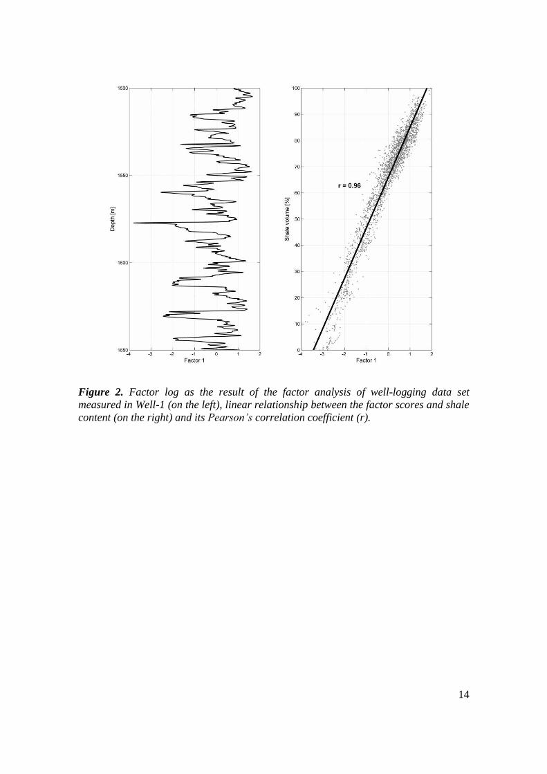
good shale indicator. In Fig. 2, the log of Factor 1 and the linear regression model of

shale content as a function of factor scores can be seen, separately. The correlation

coefficient was 0.96, which represented a straight and very strong relation between the

two variables. In Fig. 3, the shale volume logs estimated by separate petrophysical

interpretation and factor analysis based on eq. (14) can be compared. The amount of

7

fitting between the two curves was 5.4% according to eq. (16), which verified that the

independent solutions were physically the same.

6. FIELD EXAMPLE FOR NON-LINEAR CASE

In the previous section results were given for a relatively short (150m) depth interval.

A more detailed study required the processing of larger amount of data. In Fig. 4, well

logs of Well-1 can be seen, where the total number of data was 54009 in the logged

interval of 600m. It was mentioned earlier that the maximum likelihood estimation is

optimal when data follow Gaussian distribution. This condition was satisfied

sufficiently in case of this big sample. Among the applied well logs the CN, SP and AT

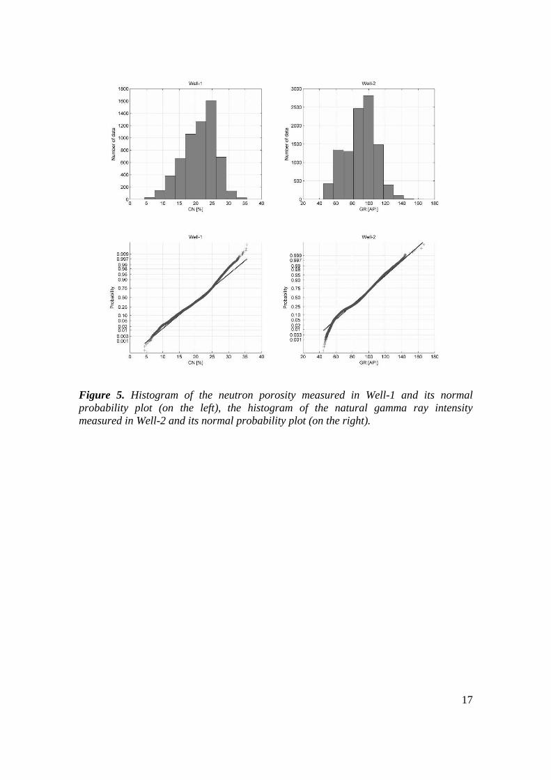
were the closest to normal distribution. As an example, the histogram of compensated

neutron data is shown in Fig. 5. In the figure, the normal probability plot of neutron data

can also be seen, where the points of the sample lie close to a straight line. The

skewness of neutron data was -0.4 and the kurtosis was -0.17 computed by eqs. (11) and

(12). The RD and CAL log having a small number of outliers were the farthest from

normal distribution. The mean of correlation coefficients computed between pairs of

well-logging data was 0.08, and that of the factors was zero after the factor analysis. In

Table 3, the extracted factor loadings can be seen. Comparing Table 2 to Table 3, it can

be noticed that in case of GR and SP logs the magnitude and sign were the same related

to Factor 1. The neutron and resistivity data as samples of original variables had bigger

weights on the factor than in the previous case. For comparing the results obtained from

different wellbores the factors were rotated by the varimax criterion and scaled. The

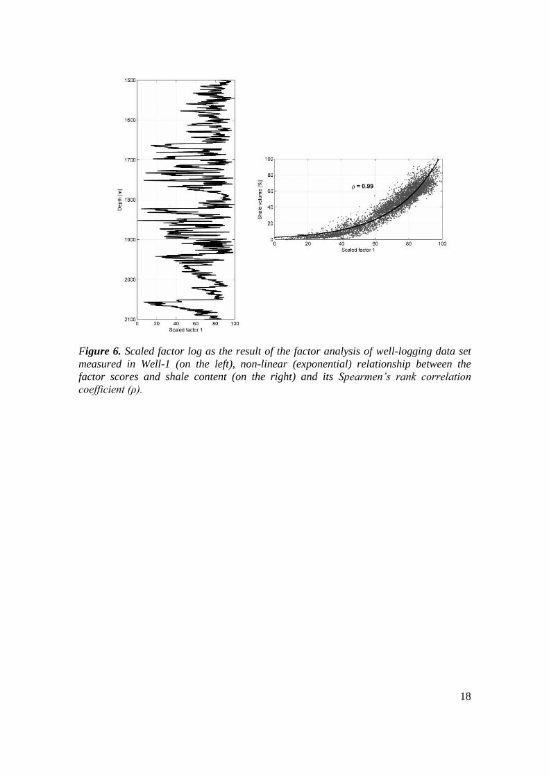
new interval of factor scores (0-100) was computed by eq. (17). In Fig. 6 the log of the

first (scaled) factor and the exponential relationship between the factor scores and shale

contents based on eq. (15) can be seen. The rank correlation coefficient between Factor

1 and shale volume was 0.99 (when assuming linear connection the Pearson’s

correlation coefficient was 0.82). Based on regression tests on additional data sets from

different boreholes of the area, the exponent b was fixed as 0.037. Afterwards, the non-

linear regression analysis of Well-1 resulted in a model specified with a=2.67. In Fig. 7,

shale volume logs estimated by separate inversion and factor analysis can be seen. The

data misfit based on eq. (16) was 8.2%, which was caused by the dispersion of data

around the model as well as the different performance of the two independent

procedures.

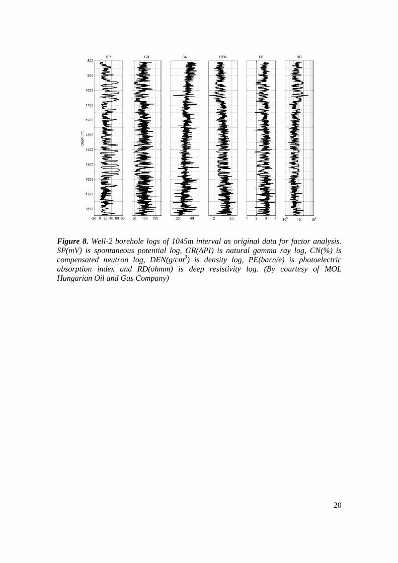
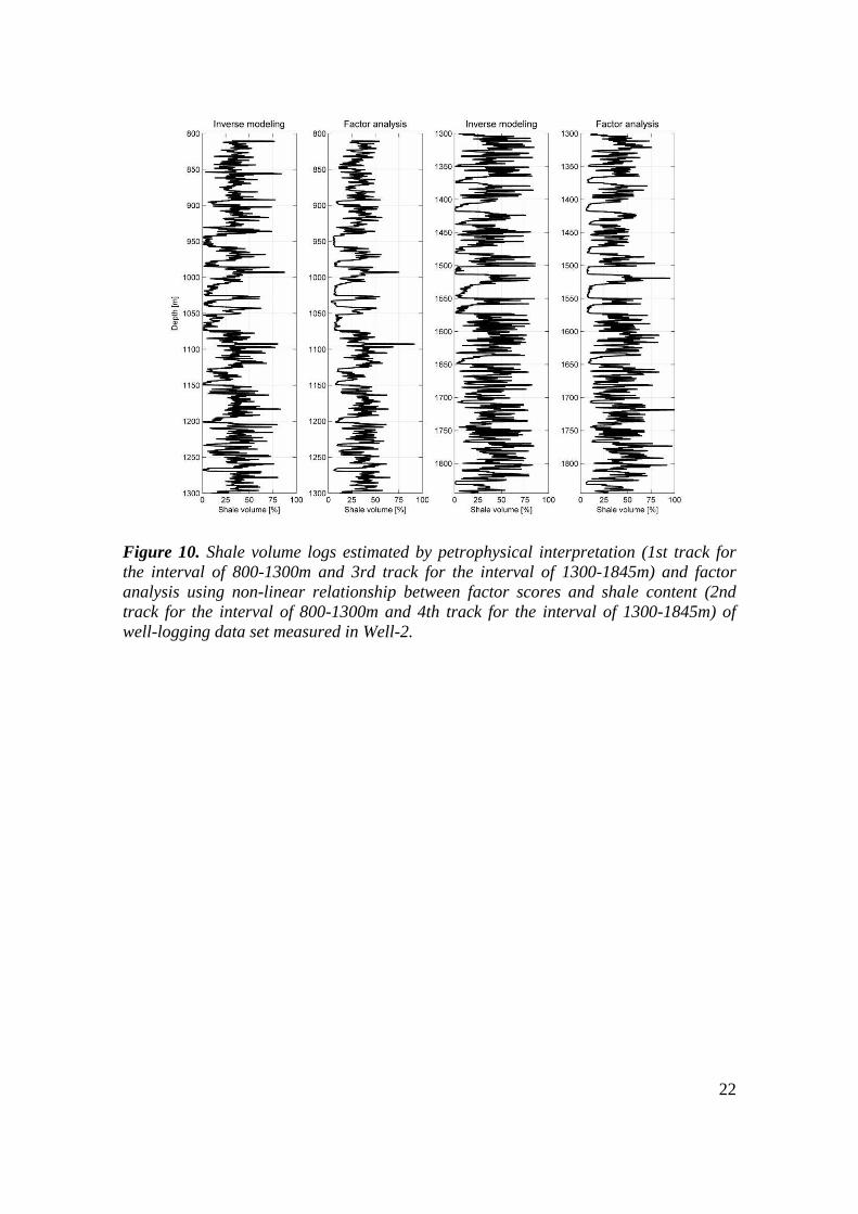
For testing the method by comparison, another well-logging data set originated from

a different area of the Great Hungarian Plain was used. In Well-2, 113861 data from a

length of 1045m logged interval were utilized (see Fig. 8). The correlation coefficient

between original data was 0.06. In case of this sample, GR, CN, PE and DEN logs were

the closest to the Gaussian distribution. For GR the skewness was -0.13 and the kurtosis

was -0.36. RD was the farthest from normal distribution again. The loadings of both

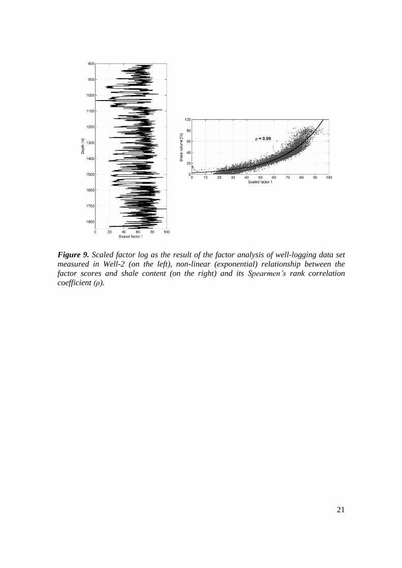
uncorrelated factors can be found in Table 4. The factors were rotated and scaled as in

case of Well-1. The magnitudes and signs of factor loadings for these two distant wells

were the same, which confirmed the feasibility of the method. Beside constant b value

(0.037), a=2.85 was given. In Fig. 9 the same model approximates to the data than was

used in Fig. 6, by the same rank correlation coefficient 0.99 (when assuming linear

connection it was 0.9). The misfit between the curves of shale volumes obtained by

inversion and factor analysis separately was 5.8% (see Fig. 10). By averaging-out the

8

values of coefficient a given by field studies done up to the present, the author suggests

the

1F037.0

sh e76.2V

(18)

formula for the estimation of shale volume in the region of the Great Hungarian Plain.

The method has been tried out both on water and hydrocarbon-bearing sedimentary

sequences, but in case of complex reservoirs, i.e. metamorphic or volcanic rocks have

not been tested. In that case not only shale but several other mineral components

constitute the matrix of rock. It is assumed that factors might be correlated to other

petrophysical properties, too.

7. CONCLUSION

Beside the quantity of information, professional practice lays ever-increasing claim

also to the quality of the interpretation results. This purpose requires advanced well-log

analysis methods. Beside deterministic and inversion procedures, new statistical

methods can also be used for extracting useful information from the well-logging data

set. It is inferred that factor analysis is applicable to extract the shale content as basic

lithological information from wellbore data. In this stage of research, we assume a non-

linear connection between the first factor and shale volume in sedimentary geological

environments. This relation proves to be straight representing a very strong correlation

between the two variables. The method gives consistent results both in water and

hydrocarbon reservoirs. Data sets from different geological areas are needed for further

research. On the other hand, data sets following non-Gaussian statistics will require a

robust procedure.

ACKNOWLEDGEMENTS

The described work was carried out as part of the TÁMOP-4.2.1.B-10/2/KONV-2010-0001 project in the framework of the New Hungarian Development Plan. The

realization of this project is supported by the European Union, co‐financed by the

European Social Fund. The author is also grateful for the support of the research team of

the Department of Geophysics, University of Miskolc and the MOL Hungarian Oil and

Gas Company for providing field data.

REFERENCES

Alberty, M., and K. Hashmy (1984), Application of ULTRA to log analysis. In: SPWLA

Symposium Transactions, New Orleans, USA, 10-13 June 1984, Society of

Petrophysicists and Well Log Analysts, Houston, paper Z, 1-17.

Asquith, G., and D. A. Krygowski (2004), Basic well log analysis, Second edition,

AAPG Methods in Exploration Series, No. 16, The American Association of Petroleum

Geologists, Tulsa, ISBN: 0-89181-667-4.

Baker Atlas (1996), OPTIMA, eXpress reference manual, Baker Atlas, Western Atlas

International, Inc. Houston.

9

Ball, S. M., D. M. Chace, and W. H. Fertl (1987), The Well Data System (WDS): An

advanced formation evaluation concept in a microcomputer environment. In: Proc. SPE

Eastern Regional Meeting, Pittsburgh, USA, 21-23 October 1987, Society of Petroleum

Engineers, Richardson, paper 17034, 61-85.

Barstow D. R. (1984), Artificial Intelligence at Schlumberger, AI Magazine, 5, 80-82.

Bartlett, M. S. (1937), The statistical conception of mental factors, British Journal of

Psychology, 28, 97–104.

Boguslavskii, M. A., and A. A. Burmistrov (2009), Petrophysical properties of

kimberlites from the Komsomolsky pipe and their relationship to its composition,

formation conditions, and diamond content, Moscow University Geology Bulletin, 64,

354–363.

Dobróka, M., and N. P. Szabó (2005), Combined global/linear inversion of well-logging

data in layer-wise homogeneous and inhomogeneous media, Acta Geodaetica et

Geophysica Hungarica, 40, 203-214.

Dolton G. L. (2006), Pannonian Basin Province, Central Europe (Province 4808) -

Petroleum geology, total petroleum systems, and petroleum resource assessment, USGS

Bulletin 2204–B, U.S. Geological Survey, Reston (Virginia), 1-47.

Fraiha, S., and J. Silva (1994), Factor analysis of ambiguity in geophysics, Geophysics,

59, 1083-1091.

Goncalves, C. A., P. K. Harvey, and M. A. Lovell (1995), Application of a multilayer

neural network and statistical techniques in formation characterization. In: SPWLA 36th

Annual Logging Symposium, Paris, France, 26-29 June 1995, Society of

Petrophysicists and Well Log Analysts, Houston, paper FF, 1-12.

Isaaks, E. H., and R. M. Srivastava (1989), An introduction to applied geostatistics,

Oxford University Press, Inc., Oxford.

Jöreskog, K. G. (2007), Factor analysis and its extensions. In: Cudeck R., and R. C.

MacCallum, Factor analysis at 100, Historical developments and future directions,

Lawrence Erlbaum Associates, Publishers, New Jersey, 47-77.

Kaiser, H. F. (1958), The varimax criterion for analytical rotation in factor analysis,

Psychometrika, 23, 187–200.

Larionov, V. V. (1969), Radiometry of boreholes (in Russian), NEDRA, Moscow.

Lawley, D. N., and A. E. Maxwell (1962), Factor analysis as a statistical method, The

Statistician, 12, 209-229.

Mayer, C., and A. Sibbit (1980), GLOBAL, a new approach to computer-processed log

interpretation. In: Proc. 55th

SPE Annual Fall Technical Conference and Exhibition,

10

Dallas, USA, 21-24 September 1980, American Institute of Mining, Mettalurgical, and

Petroleum Engineers, Dallas, paper 9341, 1-14.

Peveraro, R. C. A., and J. A. Lee (1988), HESPER: An expert system for petrophysical

formation evaluation. In: SPE European Petroleum Conference, London, UK, 16-19

October, Society of Petroleum Engineers, Richardson, 361-370.

Ranjbar, H., H. Hassanzadeh, M. Torabi, and O. Ilaghi (2001), Integration and analysis

of airborne geophysical data of the Darrehzar area, Kerman Province, Iran using

principal component analysis, Journal of Applied Geophysics, 48, 33-41.

Urbancic, T. I., and R. C. Bailey (1988), Statistical techniques applied to borehole

geophysical data, Geophysical Prospecting, 36, 752-771.

11

TABLES

Table 1. Well log types frequently used in hydrocarbon exploration

and their specification.

Code Name of well log Sensitive to Unit

SP spontaneous potential mV

GR natural gamma ray API

K Potassium per cent

U Uranium lithology ppm

Th Thorium ppm

PE photoelectric absorption barn/e

CAL caliper inch

CN compensated neutron porosity unit

DEN density porosity g/cm3

AT acoustic travel time µs/m

RMLL

RS

microlaterolog

shallow resistivity

saturation

ohmm

ohmm

RD deep resistivity ohmm

Table 2. Factor loadings derived from the well-logging data set

measured in Well-1 (150m case).

Well log Factor 1 Factor 2

CAL 0.47 -0.14

CN 0.68 -0.37

DEN 0.36 0.59

AT 0.55 -0.58

GR 0.93 0.10

RD -0.46 0.85

RMLL 0.04 0.57

RS -0.18 0.98

SP -0.85 -0.15

12




CAL 0.46 -0.02

CN 0.91 0.25

DEN 0.79 -0.60

AT 0.12 0.79

GR 0.94 -0.04

RD -0.68 -0.06

RMLL -0.72 0.57

RS -0.18 -0.01

SP -0.83 -0.15




SP -0.88 0.01

GR 0.88 -0.21

RD -0.79 -0.01

CN 0.14 -0.83

DEN 0.72 0.69

PE 0.79 0.36

13

FIGURES

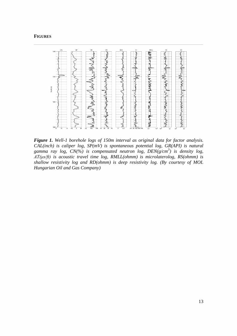
Figure 1. Well-1 borehole logs of 150m interval as original data for factor analysis.

CAL(inch) is caliper log, SP(mV) is spontaneous potential log, GR(API) is natural

gamma ray log, CN(%) is compensated neutron log, DEN(g/cm3) is density log,

AT(μs/ft) is acoustic travel time log, RMLL(ohmm) is microlaterolog, RS(ohmm) is

shallow resistivity log and RD(ohmm) is deep resistivity log. (By courtesy of MOL

Hungarian Oil and Gas Company)

14

Figure 2. Factor log as the result of the factor analysis of well-logging data set

measured in Well-1 (on the left), linear relationship between the factor scores and shale

content (on the right) and its Pearson’s correlation coefficient (r).

15

Figure 3. Shale volume logs estimated by petrophysical interpretation (on the left) and

factor analysis using Vsh=iF1 formula (on the right) of well-logging data set measured in

Well-1 (150m case).

16


CAL(inch) is caliper log, SP(mV) is spontaneous potential log, GR(API) is natural

gamma ray log, CN(%) is compensated neutron log, DEN(g/cm3) is density log,

AT(μs/ft) is acoustic travel time log, RMLL(ohmm) is microlaterolog, RS(ohmm) is

shallow resistivity log and RD(ohmm) is deep resistivity log. (By courtesy of MOL


17

Figure 5. Histogram of the neutron porosity measured in Well-1 and its normal

probability plot (on the left), the histogram of the natural gamma ray intensity

measured in Well-2 and its normal probability plot (on the right).

18

Figure 6. Scaled factor log as the result of the factor analysis of well-logging data set

measured in Well-1 (on the left), non-linear (exponential) relationship between the

factor scores and shale content (on the right) and its Spearmen’s rank correlation

coefficient (ρ).

19

Figure 7. Shale volume logs estimated by petrophysical interpretation (on the top) and

factor analysis using non-linear relationship between factor scores and shale content

(at the bottom) of well-logging data set measured in Well-1 (600m case).

20


SP(mV) is spontaneous potential log, GR(API) is natural gamma ray log, CN(%) is

compensated neutron log, DEN(g/cm3) is density log, PE(barn/e) is photoelectric

absorption index and RD(ohmm) is deep resistivity log. (By courtesy of MOL


21

Figure 9. Scaled factor log as the result of the factor analysis of well-logging data set

measured in Well-2 (on the left), non-linear (exponential) relationship between the

factor scores and shale content (on the right) and its Spearmen’s rank correlation

coefficient (ρ).

22

Figure 10. Shale volume logs estimated by petrophysical interpretation (1st track for

the interval of 800-1300m and 3rd track for the interval of 1300-1845m) and factor

analysis using non-linear relationship between factor scores and shale content (2nd

track for the interval of 800-1300m and 4th track for the interval of 1300-1845m) of

well-logging data set measured in Well-2.

shale volume estimation based on the factor analysis...

Documents