the ricean k factor: estimation and performance analysis

IEEE TRANSACTIONS ON WIRELESS COMMUNICATIONS, VOL. 2, NO. 4, JULY 2003 799

The RiceanK Factor: Estimation andPerformance Analysis

Cihan Tepedelenlioglu, Member, IEEE, Ali Abdi , Member, IEEE, and Georgios B. Giannakis, Fellow, IEEE

Abstract—In wireless communications, the relative strengthof the direct and scattered components of the received signal, asexpressed by the Ricean factor, provides an indication of linkquality. Accordingly, efficient and accurate methods for estimating

are of considerable interest. In this paper, we propose a generalclass of moment-based estimators which use the signal envelope.This class of estimators unifies many of the previous estimators,and introduces new ones. We derive, for the first time, theasymptotic variance (AsV) of these estimators and compare themwith the Cramér–Rao bound (CRB). We then tackle the problemof estimating from the in-phase and quadrature-phase (I/Q)components of the received signal and illustrate the improvementin performance as compared with the envelope-based estimators.We derive the CRBs for the I/Q data model, which, unlike theenvelope CRB, is tractable for correlated samples. Furthermore,we introduce a novel estimator that relies on the I/Q components,and derive its AsV even when the channel samples are correlated.We corroborate our analytical findings by simulations.

Index Terms—Detection and estimation, propagation andchannel characterization.

I. INTRODUCTION AND SIGNAL MODEL

I N WIRELESS communications, when there is a lineof sight (LoS) between the transmitter and the receiver,

the received signal can be written as the sum of a complexexponential and a narrowband Gaussian process, which areknown as the “LoS component” and the “diffuse component,”respectively. The ratio of the powers of the LoS component tothe diffuse component is the Ricean factor, which measures therelative strength of the LoS, and, hence, is a measure of linkquality. Consider the communication scenario in Fig. 1 wherean unmodulated carrier is transmitted, and the receiver that istraveling with a velocity receives the transmitted waveformthrough a LoS component and many multipath components.

Manuscript received December 26, 2001; revised August 23, 2002 and De-cember 9, 2002; accepted December 9, 2002. The editor coordinating the reviewof this paper and approving it for publication is P. Driessen. The work of C. Te-pedelenlioglu was supported by the National Science Foundation through Ca-reer Grant CCR-0133841, and the work of G. B. Giannakis was supported by theWireless Initiative Program under Grant 9970443 and by the NSF under Grant01-05612. This paper was presented in part at the ICASSP, Orlando, FL, 2001,and in part at the Conference on Information Systems and Sciences, Princeton,NJ, March 2002.

C. Tepedelenlioglu is with the Telecommunication Research Center, ArizonaState University, Tempe, AZ 85287 USA (e-mail: [email protected]).

A. Abdi is with the Department of Electrical and Computer Engineering,New Jersey Institute of Technology, Newark, NJ 07102 USA (e-mail:[email protected]).

G. B. Giannakis is with the Department of Electrical and ComputerEngineering, University of Minnesota, Minneapolis, MN 55455 USA (e-mail:georgios@ ece.umn.edu).

Digital Object Identifier 10.1109/TWC.2003.814338

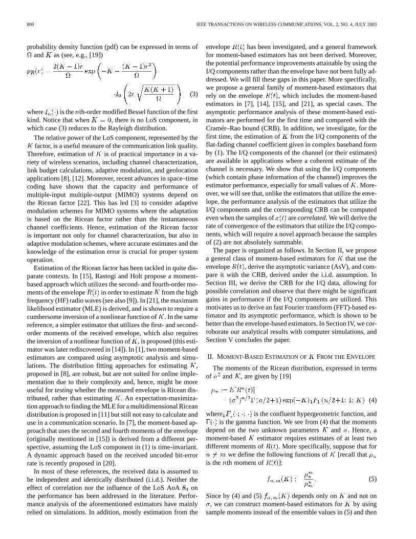
Fig. 1. Multipath propagation environment between transmitter and themobile receiver.

The baseband in-phase/quadrature-phase (I/Q) representationof the received signal can be expressed as

(1)

where is the Ricean factor and and are the angle ofarrival (AoA) and phase of the LoS respectively, and are as-sumed to be deterministic parameters. The maximum Dopplerfrequency is the ratio of the mobile velocity and the wave-length. is the diffuse component given by the sum of alarge number of multipath components, constituting a complexGaussian process. The correlation function of can be ex-pressed as (see, e.g., [19])

(2)

where denotes expectation, denotes conjugation, andis the AoA distribution of the diffuse component, which,

when uniform, yields the well-known Clarke–Jakes correlationfunction that is expressed in terms of the zeroth-order Besselfunction of the first kind: [19]. Withoutloss of generality, we are assuming which impliesthat the power of the diffuse component in (1) is. Similarly,the power of the LoS component is given by. Notice that

and in (1) are defined in such a way that the ratioyields the Ricean factor, and the received signal power isgiven by . In fact, it is often theenvelope that is of interest, and its marginal

1536-1276/03$17.00 © 2003 IEEE

800 IEEE TRANSACTIONS ON WIRELESS COMMUNICATIONS, VOL. 2, NO. 4, JULY 2003

probability density function (pdf) can be expressed in terms ofand as (see, e.g., [19])

(3)

where is the th-order modified Bessel function of the firstkind. Notice that when , there is no LoS component, inwhich case (3) reduces to the Rayleigh distribution.

The relative power of the LoS component, represented by thefactor, is a useful measure of the communication link quality.

Therefore, estimation of is of practical importance in a va-riety of wireless scenarios, including channel characterization,link budget calculations, adaptive modulation, and geolocationapplications [8], [12]. Moreover, recent advances in space–timecoding have shown that the capacity and performance ofmultiple-input multiple-output (MIMO) systems depend onthe Ricean factor [22]. This has led [3] to consider adaptivemodulation schemes for MIMO systems where the adaptationis based on the Ricean factor rather than the instantaneouschannel coefficients. Hence, estimation of the Ricean factoris important not only for channel characterization, but also inadaptive modulation schemes, where accurate estimates and theknowledge of the estimation error is crucial for proper systemoperation.

Estimation of the Ricean factor has been tackled in quite dis-parate contexts. In [15], Rastogi and Holt propose a moment-based approach which utilizes the second- and fourth-order mo-ments of the envelope in order to estimate from the highfrequency (HF) radio waves (see also [9]). In [21], the maximumlikelihood estimator (MLE) is derived, and is shown to require acumbersome inversion of a nonlinear function of. In the samereference, a simpler estimator that utilizes the first- and second-order moments of the received envelope, which also requiresthe inversion of a nonlinear function of, is proposed (this esti-mator was later rediscovered in [14]). In [1], two moment-basedestimators are compared using asymptotic analysis and simu-lations. The distribution fitting approaches for estimating,proposed in [8], are robust, but are not suited for online imple-mentation due to their complexity and, hence, might be moreuseful fortestingwhether the measured envelope is Ricean dis-tributed, rather than estimating . An expectation-maximiza-tion approach to finding the MLE for a multidimensional Riceandistribution is proposed in [11] but still not easy to calculate anduse in a communication scenario. In [7], the moment-based ap-proach that uses the second and fourth moments of the envelope(originally mentioned in [15]) is derived from a different per-spective, assuming the LoS component in (1) is time-invariant.A dynamic approach based on the received uncoded bit-errorrate is recently proposed in [20].

In most of these references, the received data is assumed tobe independent and identically distributed (i.i.d.). Neither theeffect of correlation nor the influence of the LoS AoA onthe performance has been addressed in the literature. Perfor-mance analysis of the aforementioned estimators have mainlyrelied on simulations. In addition, mostly estimation from the

envelope has been investigated, and a general frameworkfor moment-based estimators has not been derived. Moreover,the potential performance improvements attainable by using theI/Q components rather than the envelope have not been fully ad-dressed. We will fill these gaps in this paper. More specifically,we propose a general family of moment-based estimators thatrely on the envelope , which includes the moment-basedestimators in [7], [14], [15], and [21], as special cases. Theasymptotic performance analysis of these moment-based esti-mators are performed for the first time and compared with theCramér–Rao bound (CRB). In addition, we investigate, for thefirst time, the estimation of from the I/Q components of theflat-fading channel coefficient given in complex baseband formby (1). The I/Q components of the channel (or their estimates)are available in applications where a coherent estimate of thechannel is necessary. We show that using the I/Q components(which contain phase information of the channel) improves theestimator performance, especially for small values of. More-over, we will see that, unlike the estimators that utilize the enve-lope, the performance analysis of the estimators that utilize theI/Q components and the corresponding CRB can be computedeven when the samples of arecorrelated. We will derive therate of convergence of the estimators that utilize the I/Q compo-nents, which will require a novel approach because the samplesof (2) are not absolutely summable.

The paper is organized as follows. In Section II, we proposea general class of moment-based estimators forthat use theenvelope , derive the asymptotic variance (AsV), and com-pare it with the CRB, derived under the i.i.d. assumption. InSection III, we derive the CRB for the I/Q data, allowing forpossible correlation and observe that there might be significantgains in performance if the I/Q components are utilized. Thismotivates us to derive an fast Fourier transform (FFT)-based es-timator and its asymptotic performance, which is shown to bebetter than the envelope-based estimators. In Section IV, we cor-roborate our analytical results with computer simulations, andSection V concludes the paper.

II. M OMENT-BASED ESTIMATION OF FROM THE ENVELOPE

The moments of the Ricean distribution, expressed in termsof and , are given by [19]

(4)

where is the confluent hypergeometric function, andis the gamma function. We see from (4) that the moments

depend on the two unknown parametersand . Hence, amoment-based estimator requires estimates of at least twodifferent moments of . More specifically, suppose that for

we define the following functions of [recall thatis the th moment of ]:

(5)

Since by (4) and (5) depends only on and not on, we can construct moment-based estimators forby using

sample moments instead of the ensemble values in (5) and then

TEPEDELENLIOGLU et al.: RICEAN FACTOR: ESTIMATION AND PERFORMANCE ANALYSIS 801

inverting the corresponding to solve for . Hence, anestimator that depends on theth and th moments could beexpressed as

with (6)

where is the number of available samples andis the sam-pling period, and we assume that the inverse functionexists. For all the values of and we considered, isa monotone increasing function in the interval , andhence, the inverse function does exist. Notice that themoment estimator can be updated using a sliding window oflength , which would be useful in real-time estimation of.

The natural choice for is since this selectioninvolves the lowest order moments. When and ,(5) can be calculated using (4) as

(7)The corresponding estimator involves the complex nu-merical procedure of inverting (7). This estimator has been dis-cussed in [14] and its performance was studied in [21] via sim-ulations where it was found that performs similarly to theMLE. The MLE is given as the value of that satisfies the fol-lowing equation [21]:

(8)

which is evidently even more difficult to compute than ,because (7) can be inverted using a lookup table, but this is notpossible when the value of that satisfies (8) is sought forthe MLE. This is because one cannot rearrange (8) to have afunction of that does not depend on on one side of theequation, and something that only depends on the data(andnot on ) on the other side. So the MLE requires an exhaustivesearch, or a root-finding technique such as Newton’s method,where the convergence of the root estimate depend onand might not always be guaranteed.

A simpler alternative to is . It can be shown using(4) and (5) that

(9)

Solving for from an estimate of the left-hand side in (9)involves finding the roots of a second-order polynomial, whichcan be done in closed form. It can be shown that one of the rootsof this polynomial is always negative which can be discardedsince , yielding a unique nonnegative solution forwhich is given by

(10)

The estimator in (10) has been known since [9] and [15] in thecontext of HF channel modeling, and recently re-emerged in thewireless communications literature in [7], though not presented

in this general setting. In what follows, we derive novel AsVexpressions for , where and are arbitrary momentorders.

A. AsV of Moment-Based Estimators

In order to derive the AsV of the estimators proposed in thispaper, we will be using the following well-known result whichis obtained by slightly adapting [13, Th. 3.16] to our problem.

Theorem: Suppose the two statistics andconverge to and , respectively, in the mean squared sense,and the estimator of interest is given as a function of thesestatistics: . Let denotethe rate of convergence of the vector , so that

converges to a randomvector with mean zero, and covariance matrix whoseelement is given by

(11)Then, the scaled estimator

converges in distribution to a random variable withzero mean and variance given by

AsV

(12)We can now use the theorem to calculate the AsV for the mo-ment-based estimators when the envelope samples are assumedto be i.i.d. In this case, ,

, , , , and(meaning that and are -consistent becauseof the i.i.d. assumption). Using (12) and the standard result forthe derivative of an inverse function, we can express the AsV asfollows:

AsV

(13)

where is the derivative of with respect toand can be computed using (4) and (5). Hence, we can concludethat all moment-based estimators in (6) are -con-sistent, and asymptotically unbiased, with AsV given by (13).Notice that (13) is a function of only and does notdepend on . This can easily be seen from the fact that the esti-mator in (6) is scale invariant (i.e., if the envelope data is multi-plied by a constant, the estimator in (6) remains the same).

In order to compare the AsV expression in (13) with a bench-mark, we numerically computed the CRB, which provides alower bound for the variance of any unbiased estimator. TheCRB was reported in [21] as

CRB (14)


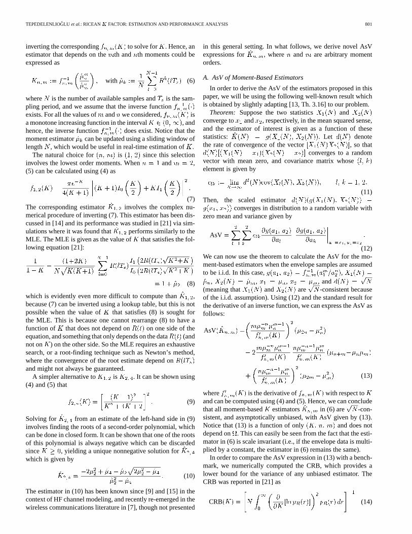
Fig. 2. Asymptotic performance of envelope-basedK estimators and CRB.

but this expression assumes that the only unknown is, andthat is known. The CRB for the more realisticscenario that is unknown can be derived from the Fischerinformation matrix (FIM) of by using the (1,1) elementof the inverse FIM, and is shown to be greater than the CRB forthe known , which is a well-known consequence ofbeinga nuisance parameter [10]. We show in Appendix A how this isdone numerically. It is important to point out that whetherisknown or not affects the CRB. However, thevalueof does notaffect the CRB, because the CRB is scale invariant, and, hence,does not depend on the second moment.

Fig. 2 plots the asymptotic standard deviation (square root ofthe AsV) for , , and , as well as the square rootof the CRB for known and unknown, which collectively il-lustrate the performance of moment-based estimators for largesample sizes. As expected, the CRB for knownis smallerthan the CRB for unknown , even though the difference isvery small. In the rest of this section, unless otherwise noted,CRB will refer to the realistic case where is unknown. No-tice from Fig. 2 that as gets smaller, making the Ricean pdfmore like Rayleigh, no unbiased envelope-based estimator canestimate accurately because the CRB goes to infinity. Wealso observe that the most accurate estimation offrom theenvelope is possible around . Note also that as

increases, the asymptotic standard deviation goes to infinityapproximately linearly. Among the moment-based estimators,

(dashed line) has the least AsV for moderate/large, andis in fact indistinguishable from the CRB for , whichleads us to conclude that isalmostasymptotically efficient.As we expected, increasing and (implying usage of higherorder moments) result in larger AsV for moderate/large. In-deed, the simple estimator in (10), for which there is aclosed form expression, and have a greater AsV than thatof .

After we have introduced and analyzed the family of estima-tors that utilize the envelope samples, we notice that two

of these estimators are noteworthy: has the best asymp-totic performance of all the moment-based estimators with in-teger moments, which is indistinguishable from the CRB, and

in (10) has a simple closed-form solution which is easierto implement in practice.

III. ESTIMATION OF FROM THE I/Q COMPONENTS

In this section, we will investigate the estimation offromthe I/Q components of the received signal given in complexbaseband form, which are the real and imaginary parts of (1).To the best of our knowledge, this is the first estimator ofthatuses the I/Q components. The I/Q components are available inapplications where a coherent estimate of the channel is neces-sary. We will show that using the I/Q components (which con-tain envelopeandphase information of the channel) improvesthe estimator performance, especially for small values of.

A. CRB for I/Q Data

In this section, we will derive the CRB for the variance ofestimators that use the I/Q data in (1). The resulting CRB willbe a lower bound on the variance of any unbiased estimator for

obtained not only from the I/Q components in (1), but alsofrom the envelope. This is because any estimator that can be con-structed from the envelope can be constructed from (1). We willsee that unlike the derivation of the envelope CRB, we will notneed to make the restrictive i.i.d. assumption when deriving theI/Q CRB because of the tractability of the multivariate Gaussianpdf (as opposed to the difficulty of expressing and working withthe multivariate Ricean pdf that emerges with correlated enve-lope samples). CRBs for fading parameters for a differently pa-rameterized radio transmission channel can also be found in [5].

Let us define the -spaced samples of (1) as ,and . We may then

express the sampled I/Q signal in terms ofand as follows:

(15)

Suppose that we have a data record ofsamples from (15).We would like to compute the CRB for the parameter. Weemphasize that the I/Q CRB in this section is different from theenvelope CRB, because the data from which they are derivedare different. We will calculate the I/Q CRB for two cases.

1) All the parameters (except ) are known.2) All parameters in are unknown and

the channel correlations are given by, where .

The first case, which appears rather unrealistic, is importantbecause it provides a lower bound onany estimator ofwhether any other parameter is known or not, and whether theenvelope or the I/Q components are used. Another reason forconsidering Case 1 is the resulting simplicity of the bound. Weshall consider Case 1 first, and then we will address Case 2.

Let be a length- vector that con-tains the available sampled I/Q components, and

. Then the meanand covariance matrix of are given by

, and


, where denotes the normalized1 covariancematrix of the I/Q components, and denotes Hermittian. Whenall parameters in except are known (Case 1), using (33) inAppendix B, it is easy to show that

CRB (16)

which reduces to the simple when s are independent(i.e., when ).

Some remarks are now in order.Remark 1: Note that if the correlations satisfy

, then we can use the standard results for theasymptotic forms of Toeplitz matrices (see, e.g., [6]) to concludethat the asymptotic CRB defined as CRBconverges to , for , where is thespectrum of . The absolute summability of the covarianceshold, for example, when is modeled as an autoregressiveprocess. We see that, in this case, if is large, the CRBincreases. However, the correlation function we have adoptedin (2), which is a more accurate correlation model for wirelesscommunications, is not absolutely summable in general, sowe cannot easily establish the link between and theasymptotic CRB in Case 1, as we did whenholds.

Remark 2: The CRB in (16) considers only as an un-known parameter, which yields a bound that is smaller than theCRB when other parameters of the model in (15) are unknown.Hence, (16) provides a lower bound to the variance ofanyunbi-ased estimator of , regardless of whether it is constructed fromthe envelope or the I/Q components of the signal, or whether anyof the other parameters are known.

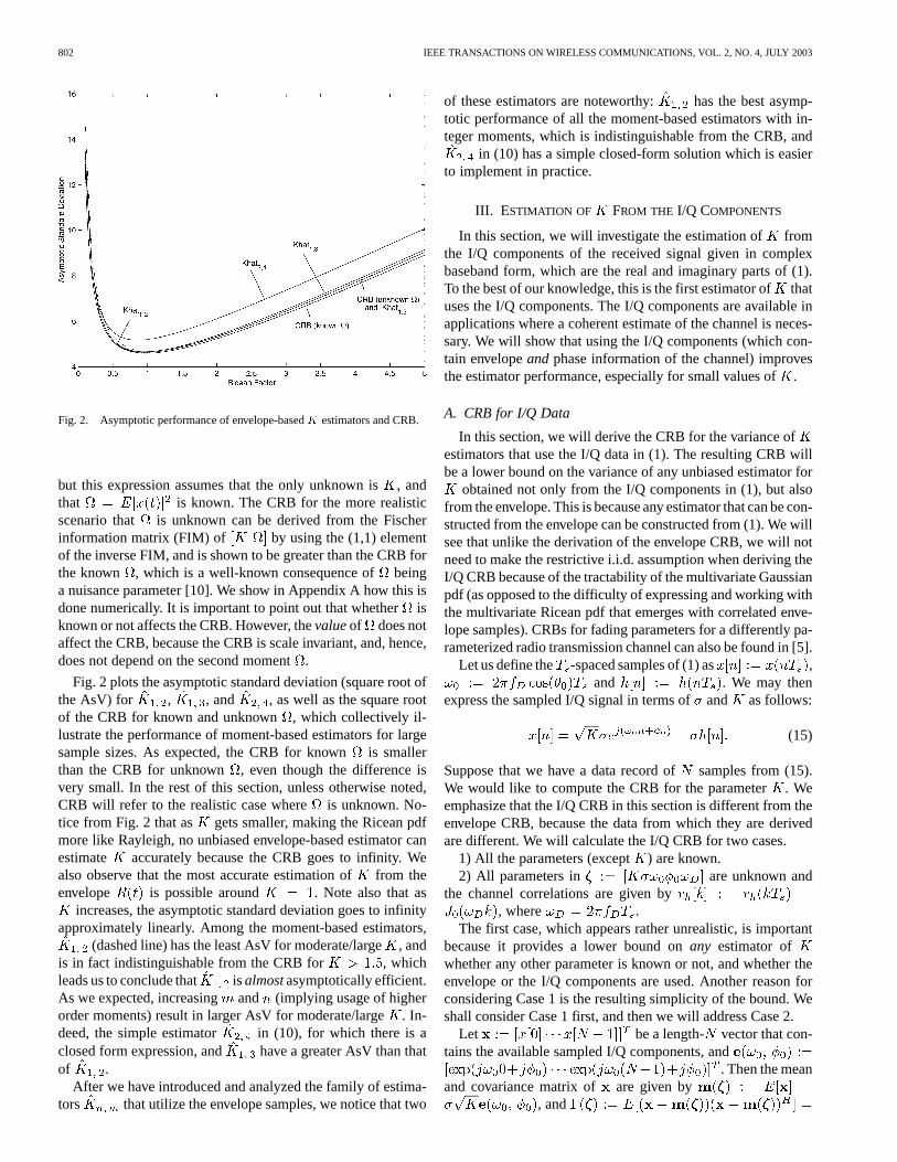
Remark 3: Unlike the envelope CRB in Fig. 2, as getssmaller, the I/Q CRB in (16) goes to zero. This is also the casefor the CRB for the more realistic Case 2, whereis unknown,which is derived in Appendix B [see (35)]. In Fig. 3, we showthe CRB for the envelope data model, CRB for Case 1 in (16)where the parameters are known, and the CRB for Case 2 in(35) where the parameters are unknown. We observe in Fig. 3that CRBs for the I/Q data become smaller asgets smaller forboth Cases 1 and 2, which is also proved in the Appendix B forboth cases. This reinforces our intuition that the additional phaseinformation in the I/Q data, which is not present in the envelopedata, offers potential improvements in estimator performance,particularly for small . This insight motivates us to search forestimators of from the I/Q components. We now propose suchan estimator.

B. Estimator of From the I/Q Components

In pursuit of finding an estimator for from the I/Q compo-nents, the first thing that comes to mind is the MLE constructedfrom the I/Q data (which is different from (8) constructed fromthe envelope data). But an MLE from the I/Q data will have to in-volve joint estimation of , and , which requiresa multidimensional search and, hence, is not practical. An alter-native to the MLE is a nonlinear least-squares approach of [18],

1So that it has ones on the main diagonal.

Fig. 3. Different CRBs forK.

which was proposed to estimate, , , and , but not . Inwhat follows we provide a yet simpler approach.

Let . Consider nowthe following statistics of :

(17)

(18)

Let us assume, for the moment, that . Recalling that, and substituting it in (17), we

arrive at . Sinceas seen from (20), goes to zero in themean-squared sense asincreases, we see that for sufficientlylarge , . On the other hand, in (18) con-verges to . This prompts us to propose the followingestimator for that approximates :

(19)

Compared with the estimators that rely on the envelope, the I/Qestimator requires a step to estimate, which can be accom-plished with FFT complexity . Hence, the penaltypaid for the performance improvements that the I/Q estimatoroffers is a slight increase in computational complexity. Similarto the moment-based estimators, the I/Q estimator can benefitfrom updating and using a sliding window forapplications requiring estimates of in real-time. We will nowderive the AsV of (19).

C. AsV of

In this section, we calculate the AsV of for the casewhen the samples are independent, and also when theyare correlated. To simplify the analysis, we will assume that

. Hence, our calculations will yield the AsV when isknown perfectly, which is a lower bound to the AsV of (19). We


will begin with the case where the samples are independent.Let , [c.f. (19)],

and (because (17) converges to and(18) converges to ). To calculate the in (11), we will usethe following covariance expressions which are straightforwardto show [23]:

(20)

(21)

(22)

where and denotes real part. Using(20)–(22) with ,2 we obtain ,

, and . Differ-entiating we get ,

and substituting in (12), and sim-plifying, we finally obtain

AsV (23)

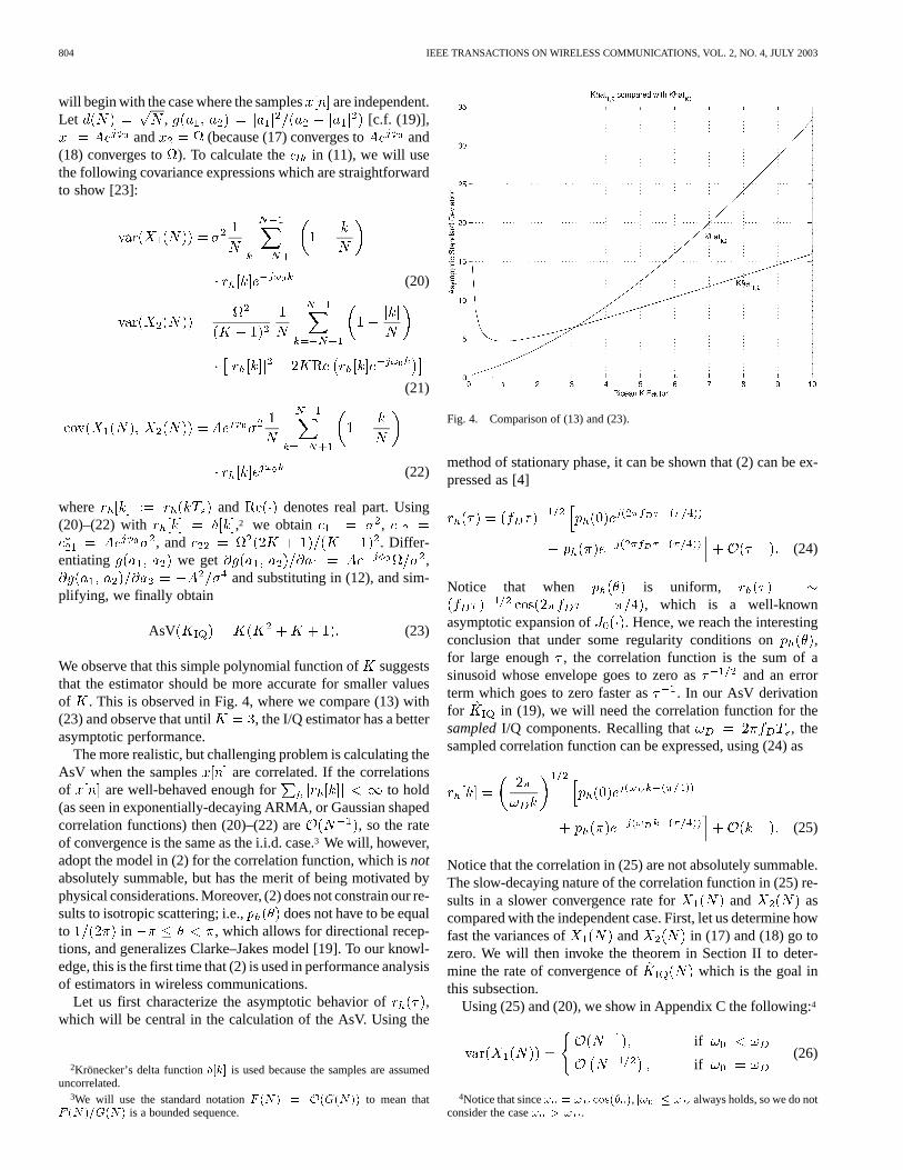
We observe that this simple polynomial function ofsuggeststhat the estimator should be more accurate for smaller valuesof . This is observed in Fig. 4, where we compare (13) with(23) and observe that until , the I/Q estimator has a betterasymptotic performance.

The more realistic, but challenging problem is calculating theAsV when the samples are correlated. If the correlationsof are well-behaved enough for to hold(as seen in exponentially-decaying ARMA, or Gaussian shapedcorrelation functions) then (20)–(22) are , so the rateof convergence is the same as the i.i.d. case.3 We will, however,adopt the model in (2) for the correlation function, which isnotabsolutely summable, but has the merit of being motivated byphysical considerations. Moreover, (2) does not constrain our re-sults to isotropic scattering; i.e., does not have to be equalto in , which allows for directional recep-tions, and generalizes Clarke–Jakes model [19]. To our knowl-edge, this is the first time that (2) is used in performance analysisof estimators in wireless communications.

Let us first characterize the asymptotic behavior of ,which will be central in the calculation of the AsV. Using the

2Krönecker’s delta function�[k] is used because the samples are assumeduncorrelated.

3We will use the standard notationF (N) = O(G(N)) to mean thatF (N)=G(N) is a bounded sequence.

Fig. 4. Comparison of (13) and (23).

method of stationary phase, it can be shown that (2) can be ex-pressed as [4]

(24)

Notice that when is uniform,, which is a well-known

asymptotic expansion of . Hence, we reach the interestingconclusion that under some regularity conditions on ,for large enough , the correlation function is the sum of asinusoid whose envelope goes to zero as and an errorterm which goes to zero faster as . In our AsV derivationfor in (19), we will need the correlation function for thesampledI/Q components. Recalling that , thesampled correlation function can be expressed, using (24) as

(25)

Notice that the correlation in (25) are not absolutely summable.The slow-decaying nature of the correlation function in (25) re-sults in a slower convergence rate for and ascompared with the independent case. First, let us determine howfast the variances of and in (17) and (18) go tozero. We will then invoke the theorem in Section II to deter-mine the rate of convergence of which is the goal inthis subsection.

Using (25) and (20), we show in Appendix C the following:4

if

if(26)

4Notice that since! = ! cos(� ), j! j � ! always holds, so we do notconsider the case! > ! .


and similarly, using (25) and (21), we show in Appendix C that

if

if(27)

Comparing (20) and (22), it is apparent that andconverge at the same rate given by (26).

Recall that when the samples are independent (or moregenerally, when ), the convergence rate of thevariances of both and is . Itis interesting that, for correlation functions of the form in (2),the rate of convergence of both and depends onwhether . Physically, when in (1),i.e., the LoS is in the same direction as the mobile. So, when

, converges faster than , and when, the variances of and converge to

zero at the same rate. Now we are ready to invoke the theoremof Section II.

The theorem requires that both and shouldconverge when scaled by the same sequence. So, when

, the scaling sequence should be the slower of theand , so that the faster one will converge to zero (if wewere to scale with the rate of the faster one, the slower statisticwould go to infinity). Hence, when , we choose

so that . To calculate the AsV,we need to substitute in (12), , the partialderivatives of , which are given right before (23), and

, which, using (11), (20)–(22), (26), and (27), are given by, and , where

and the resulting AsV are given by

AsV

(28)

and the limit , which is independent of , can be shownto exist using (25). When , we have that both

and converge at the same rate. So we selectand substitute in (12) , the

partial derivatives, and , which, using (11) and (20)–(27),turn out to be , , and

, where and the resulting AsVare given by

AsV

(29)

and the limit is independent of .

Hence, loosely speaking, we can say that when the dataare independent, the AsV of is proportional to

when the estimator is scaled by. When the data are correlated with correlation function

given in (2), we have the case : the AsV ofis proportional to when the estimator is scaled

by , and we have the case :the AsV of is proportional to when theestimator is scaled by .

Some conclusions that we can draw from this analysis are asfollows. Regardless of whether the data samples are correlatedor not, the becomes more accurate if is small. In fact,our motivation for pursuing the estimation of from theI/Q components was precisely this reason; while all unbiasedestimators of from the envelope yield an unbounded varianceas gets smaller, the accuracy of increases with smaller

. It is also important to notice that the value of makesa difference in the performance, so much so that it makes adifference in therate of convergence. In fact even for finite

, motivated by Remark 1 following (16), values of forwhich is small, yield better performance. If we adoptthe isotropic scattering model, corresponding to a uniform

, . Sinceis infinite, when the performance is worse

as compared with when . This spectrum has aminimum at zero; hence, (implying ) seemsto be the best AoA for the LoS component as far as theperformance of is concerned. Physically, this is a LoSthat is perpendicular to the direction of the mobile yieldinga time-invariant LoS component.

IV. SIMULATIONS

In this section, we provide a computer simulation study ofthe various estimators. The signal from which thefactor isestimated has been generated using a sum of sinusoids modelthe details of which can be found in [23].

A. Envelope-Based Estimators: Comparison With the MLEand Effect of Finite Sample Size

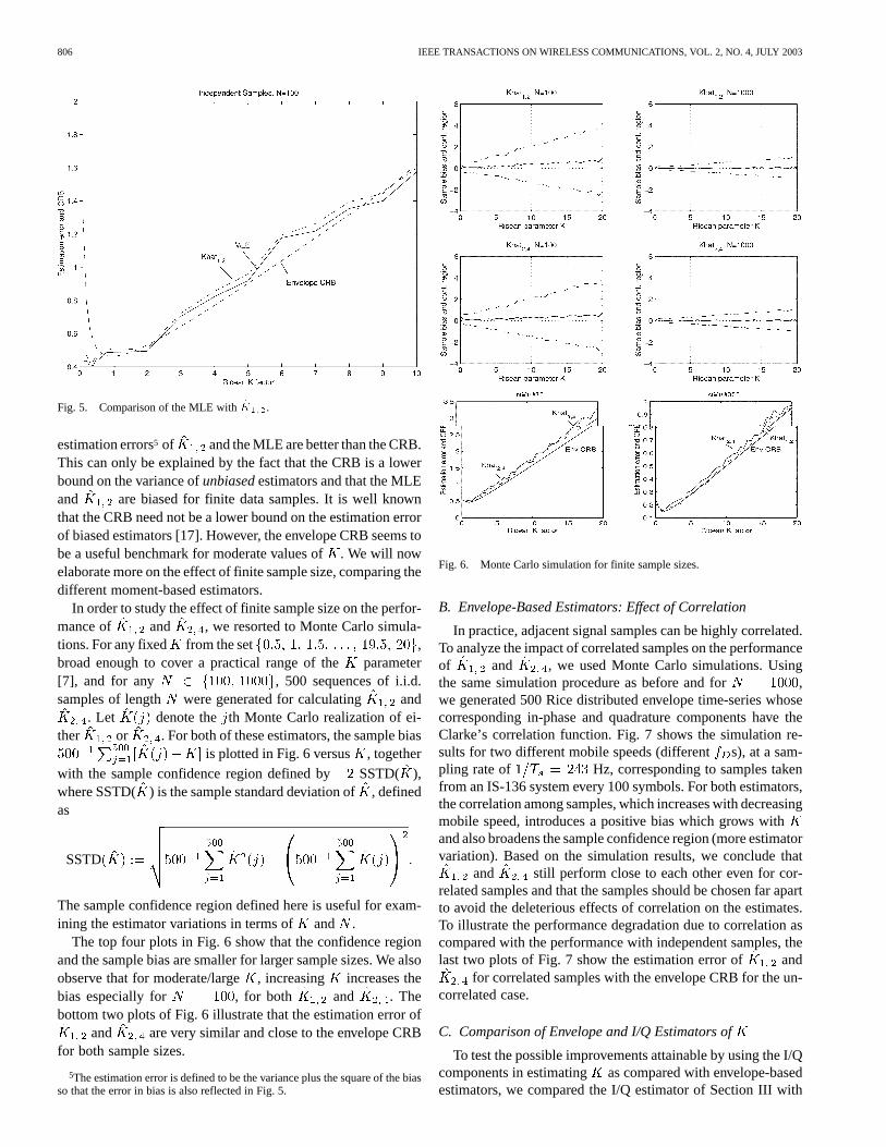
The MLE of for the envelope data is given in (8) and isknown to be very close to the CRB for large number of datasamples. Since is also very close to the CRB, as evidencedby Fig. 2, we know that the moment-based estimators performsimilar to the MLE for large . In order to answer the questionof how the moment-based estimators compare with the MLEfor finite data samples, we show the performance of alongwith the MLE in Fig. 5 for . The MLE was calculatingusing an exhaustive search for the value ofthat satisfies (8).We observe that even for small values of, the MLE is onlyslightly better than the simpler moment-based estimator. Thesame trend was observed even when the envelope samples werecorrelated (not shown). We have also plotted the envelope CRBin Fig. 5 for reference. We observe that for small values of, the


Fig. 5. Comparison of the MLE with^K .

estimation errors5 of and the MLE are better than the CRB.This can only be explained by the fact that the CRB is a lowerbound on the variance ofunbiasedestimators and that the MLEand are biased for finite data samples. It is well knownthat the CRB need not be a lower bound on the estimation errorof biased estimators [17]. However, the envelope CRB seems tobe a useful benchmark for moderate values of. We will nowelaborate more on the effect of finite sample size, comparing thedifferent moment-based estimators.

In order to study the effect of finite sample size on the perfor-mance of and , we resorted to Monte Carlo simula-tions. For any fixed from the set ,broad enough to cover a practical range of theparameter[7], and for any , 500 sequences of i.i.d.samples of length were generated for calculating and

. Let denote the th Monte Carlo realization of ei-ther or . For both of these estimators, the sample bias

is plotted in Fig. 6 versus , togetherwith the sample confidence region defined by SSTD( ),where SSTD( ) is the sample standard deviation of, definedas

SSTD

The sample confidence region defined here is useful for exam-ining the estimator variations in terms of and .

The top four plots in Fig. 6 show that the confidence regionand the sample bias are smaller for larger sample sizes. We alsoobserve that for moderate/large, increasing increases thebias especially for , for both and . Thebottom two plots of Fig. 6 illustrate that the estimation error of

and are very similar and close to the envelope CRBfor both sample sizes.

5The estimation error is defined to be the variance plus the square of the biasso that the error in bias is also reflected in Fig. 5.

Fig. 6. Monte Carlo simulation for finite sample sizes.

B. Envelope-Based Estimators: Effect of Correlation

In practice, adjacent signal samples can be highly correlated.To analyze the impact of correlated samples on the performanceof and , we used Monte Carlo simulations. Usingthe same simulation procedure as before and for ,we generated 500 Rice distributed envelope time-series whosecorresponding in-phase and quadrature components have theClarke’s correlation function. Fig. 7 shows the simulation re-sults for two different mobile speeds (different s), at a sam-pling rate of Hz, corresponding to samples takenfrom an IS-136 system every 100 symbols. For both estimators,the correlation among samples, which increases with decreasingmobile speed, introduces a positive bias which grows withand also broadens the sample confidence region (more estimatorvariation). Based on the simulation results, we conclude that

and still perform close to each other even for cor-related samples and that the samples should be chosen far apartto avoid the deleterious effects of correlation on the estimates.To illustrate the performance degradation due to correlation ascompared with the performance with independent samples, thelast two plots of Fig. 7 show the estimation error of and

for correlated samples with the envelope CRB for the un-correlated case.

C. Comparison of Envelope and I/Q Estimators of

To test the possible improvements attainable by using the I/Qcomponents in estimating as compared with envelope-basedestimators, we compared the I/Q estimator of Section III with


Fig. 7. Monte Carlo simulation for correlated samples.

Fig. 8. Comparison of envelope-based and I/Q-based estimators and CRB.

the envelope-based . We chose data points and, which corresponds to a vehicle velocity of

km/h, s, and a carrier frequency of 900 MHz.We observe from Fig. 8 that the estimator that relies on the I/Qcomponents performs significantly better than . Moreover,the I/Q CRB provides a tight lower bound on the estimation errorof the I/Q estimator particularly for small values of. This is

at the expense of a slight increase in computational complexity,and the necessity of measuring the I/Q components of the re-ceived signal.

V. CONCLUSION

We started out by proposing a new family of estimators forfrom the envelope samples. This general class of estimators wasshown to unify the existing approaches in the literature. We de-rived the AsV of each member of this family of moment-basedestimators and showed that they perform close to the CRB.Two moment-based estimators and were worthyof special attention because had the best asymptoticperformance, and had a simple closed-form expressionin terms of the moments. It was mentioned that a real-timelow-complexity implementation of these estimators shoulduse a sliding window approach to estimating the necessarymoments.

Motivated by the fact that the envelope CRB increaseswithout bound as gets smaller, we studied the estimation of

from the I/Q data. We observed that the I/Q CRB goes tozero as gets smaller, a property also held by the AsV of anovel I/Q-based estimator that we proposed. The performanceanalysis for this estimator for correlated samples yieldedinsights into the effect of on the estimator performance. Thesimulations corroborate the analytical findings of the previoussections and illustrate that the moment-based estimators thatuse the envelope are very close to the MLE even for finitesample sizes, and that outperforms .

We conclude that among the moment-based estimators fromthe envelope, is computationally simpler than , at theexpense of a loss in performance. We also suggest that the I/Qcomponents be used when they are available for estimation of

because they offer an improvement in performance over theenvelope-based estimators.

APPENDIX ACRB FOR ENVELOPE-BASED ESTIMATORS

It is straightforward to show the following:

(30)

(31)


Let denote the entry of a generic matrix .Defining the FIM entries as

we can express the CRB for the envelope data for unknownas the (1,1) element of the inverse FIM, which is easily shownto be

CRB (32)

Notice that the entries of the FIM need to be computed withnumerical integration using (31). Notice also that (14) is givenby , and is smaller than or equal to (32) because

in (32).

APPENDIX BCRB FOR I/Q-BASED ESTIMATORS

For I/Q data which is complex Gaussian with mean andcovariance matrix , the elements of the FIM are given by[26]

(33)

where denotes the th element of , and denotes thetrace of a matrix.

We now calculate the CRB for estimators of that use theI/Q components, assuming that all the elements inare un-known. For this, we need the partial derivatives of and

with respect to , which are given in the following

(34)

where. Using (34) and (33), all entries of the

FIM can be computed, and the (1,1) element of the inverse FIMwill be the CRB of estimators that utilize the I/Q componentswhen is unknown. Let for brevity. An impor-tant point is that is proportional to and, hence, goesto infinity as goes to zero. Also, the submatrixconsisting of the second through fifth row, and second throughfifth column of , stays constant as goes to zero. Thiscan be easily verified using (34) and (33). Furthermore, let

and be vectors consisting of the secondthrough fifth column of the first row and second through fifthrow of the first column, respectively. Then, as a consequenceof the matrix inversion lemma [16, p. 512], the (1,1) element ofthe inverse FIM (which is the CRB of interest) is given by

(35)

As goes to zero, goes to infinity, and all the other termsremain bounded, which shows that in (35), which isthe CRB of interest, and goes to zero asgoes to zero.

APPENDIX CRATES OFCONVERGENCE

In this appendix, we will derive (26) and (27). In order toshow (26) for , we need to show thatconverges to a finite constant. To show that con-verges, we need to establish

for which it suffices to show thatbecause of the Cesaro summability theorem [13, p. 411]. Sub-stituting (25) for , we can writewhere

(36)

and the approximation is due to the term in (25). Wecan now apply Drichlet’s test [2, p. 365], which states that if

converges monotonically to zero and the partial sums ofare bounded, then converges. Since these two

conditions hold in our case ( ), we conclude that, which is what we needed to show.

Let us now show that (26) for holds. To do this,we need to show that

(37)

where and are obtained by substitutingin (36) and are given by ,


,which is the sum of a constant and an exponential, but

and add upto (37), and they are both . This can be seen aftersubstituting for and , and using the following:6

, and ,where the first two equalities are obtained by integratingand , respectively, and the third expression is obtainedusing Drichlet’s theorem. This establishes the equality in (37)which is what we wanted to show.

We will now show that (27) holds. For , we needto show that

(38)

which would establish that (21) is . We knowfrom (26) that for , converges; hence,we can do away with the second term in the square brackets in(38), and see that establishing (38) amounts to showing

(39)

Using (25), it is straightforward to show that the first term onthe left-hand side of (39) is

(40)

which is , where the term is ob-tained by integrating , and the term is obtained byusing Drichlet’s theorem, but the second term on the left-handside of (39) is , which canbe verified similar to (40). So (39) must be . This es-tablishes what we wanted to show.

Using a similar approach, it is not difficult to show that forthe case , (38) is given by

, which completes the derivations of (26) and (27).

ACKNOWLEDGMENT

The authors would like to thank M. Kaveh of the Universityof Minnesota for his valuable comments and insight.

6Since we are interested in asymptotic expressions for largeN , we are notconcerned with the fact thatk is unbounded fork = 0.

REFERENCES

[1] A. Abdi, C. Tepedelenlioglu, G. B. Giannakis, and M. Kaveh, “On theestimation of theK parameter for the Rice fading distribution,”IEEECommun. Lett., vol. 5, pp. 92–94, Mar. 2001.

[2] T. M. Apostol, Mathematical Analysis. Reading, MA: Ad-dison-Wesley, 1957.

[3] S. Catreux, V. Erceg, D. Gesbert, and R. W. Heath, “Adaptive modu-lation and MIMO coding for broadband wireless data networks,”IEEECommun. Mag., vol. 40, pp. 108–115, June 2002.

[4] E. T. Copson,Asymptotic Expansions. Cambridge, U.K.: CambridgeUniv. Press, 1965.

[5] F. Gini, M. Luise, and R. Reggiannini, “Cramér–Rao bounds in the para-metric estimation of fading radio transmission channels,”IEEE Trans.Commun., vol. 46, pp. 1390–1398, Oct. 1998.

[6] R. Gray. (2001) Toeplitz and circulant matrices: A review. [Online].Available: http://www-ee.stanford.edu/~gray/toeplitz.html.

[7] L. J. Greenstein, D. G. Michelson, and V. Erceg, “Moment-methodestimation of the RiceanK-factor,” IEEE Commun. Lett., vol. 3, pp.175–176, June 1999.

[8] D. Greenwood and L. Hanzo, “Characterization of mobile radio chan-nels,” inMobile Radio Communications, R. Steele, Ed. London, U.K.:Pentech, 1992, pp. 92–185.

[9] W. K. Hocking, “Reduction of the effects of nonstationarity in studiesof amplitude statistics of radio wave backscatter,”J. Atmos. Terr. Phys.,vol. 49, no. 11/12, pp. 1119–1131, 1987.

[10] E. L. Lehmann and G. Casella,Theory of Point Estimation, 2nded. New York: Springer-Verlag, 1998.

[11] T. L. Marzetta, “EM algorithm for estimating the parameters of a multi-variate complex Ricean density for polarimetric SAR,” inProc. ICASSP,Detroit, MI, 1995, pp. 3651–3654.

[12] K. Pahlavan, P. Krishnamurthy, and A. Beneat, “Wideband radio prop-agation modeling for indoor geolocation applications,”IEEE Commun.Mag., vol. 36, pp. 60–65, Apr. 1998.

[13] B. Porat,Digital Processing of Random Signals. Englewood, NJ: Pren-tice-Hall, 1994.

[14] F. van der Wijk, A. Kegel, and R. Prasad, “Assessment of a pico-cellularsystem using propagation measurements at 1.9 GHz for indoor wirelesscommunications,”IEEE Trans. Veh. Technol., vol. 44, pp. 155–162, Feb.1995.

[15] P. K. Rastogi and O. Holt, “On detecting reflections in presence of scat-tering from amplitude statistics with application toD region partial re-flections,”Radio Sci., vol. 16, no. 6, pp. 1431–1443, 1981.

[16] T. Söderström and P. Stoica,System Identification. Englewood Cliffs,NJ: Prentice-Hall, 1989.

[17] P. Stoica and R. Moses, “On biased estimators and the unbiased CRB,”Signal Process., vol. 21, no. 4, pp. 349–350, 1990.

[18] P. Stoica, A. Jakobsson, and J. Li, “Cisoid parameter estimation in thecolored noise case: asymptotic Cramér–Rao bound, maximum likeli-hood, and nonlinear least-squares,”IEEE Trans. Signal Processing, vol.45, pp. 2048–2059, Aug. 1997.

[19] G. L. Stüber,Principles of Mobile Communication. Norwell, MA:Kluwer, 1996.

[20] M. Sumanasena and B. Evans, “Rice factor estimation algorithm,”Elec-tron. Lett., vol. 37, no. 14, pp. 918–919, 2001.

[21] K. K. Talukdar and W. D. Lawing, “Estimation of the parameters of theRice distribution,”J. Acoust. Soc. Amer., vol. 89, no. 3, pp. 1193–1197,1991.

[22] V. Tarokh, N. Seshadri, and A. R. Calderbank, “Space–time codes forhigh data rate wireless communication: Performance criterion and codeconstruction,”IEEE Trans. Inform. Theory, vol. 44, pp. 744–765, Mar.1998.

[23] C. Tepedelenlioglu and G. B. Giannakis, “On velocity estimation andcorrelation properties of narrowband communication channels,”IEEETrans. Veh. Technol., vol. 50, pp. 1039–1052, July 2001.

[24] C. Tepedelenlioglu, A. Abdi, G. Giannakis, and M. Kaveh, “Perfor-mance analysis of moment-based estimators for theK parameter of theRice fading distribution,” inProc. ICASSP, vol. 4, 2001, pp. 2521–2524.

[25] C. Tepedelenlioglu and A. Abdi, “Estimation of the Rice factor fromthe I/Q components,” inProc. Conf. Information Systems Sciences, Mar.2002, pp. 423–428.

[26] A. Zeira and A. Nehorai, “Frequency domain Cramér–Rao bound forGaussian processes,”IEEE Trans. Acoust., Speech, Signal Processing,vol. 38, pp. 1063–1066, June 1990.


Cihan Tepedelenlioglu (S’97–M’01) was bornin Ankara, Turkey, in 1973. He received the B.S.degree (with highest honors) from the FloridaInstitute of Technology, Melbourne, in 1995, andthe M.S. degree from the University of Virginia,Charlottesville, in 1998, both in electrical engi-neering. He received the Ph.D. degree in electricaland computer engineering from the University ofMinnesota, Minneapolis, in 2001.

From January 1999 to May 2001, he was a Re-search Assistant at the University of Minnesota. He is

currently an Assistant Professor of electrical engineering at the Telecommunica-tions Research Center, Arizona State University, Tempe. His research interestsinclude statistical signal processing, system identification, wireless communi-cations, estimation and equalization algorithms for wireless systems, filterbanksand multirate systems, carrier synchronization for wireless LANs, power esti-mation, and handoff algorithms.

Dr. Tepedelenlioglu won the NSF early Career Award in 2001.

Ali Abdi (S’98–M’01) received the Ph.D. degree inelectrical engineering from the University of Min-nesota, Minneapolis, in 2001.

He joined the Department of Electrical andComputer Engineering of the New Jersey Institute ofTechnology (NJIT), Newark, in 2001, as an AssistantProfessor. His previous research interests haveincluded stochastic processes, wireless communica-tions, pattern recognition, neural networks, and timeseries analysis. His current work is mainly focusedon wireless communications, with special emphasis

on modeling, estimation, and simulation of wireless channels, multiantennasystems, and system performance analysis.

Dr. Abdi is an Associate Editor for IEEE TRANSACTIONS ON VEHICULAR

TECHNOLOGY.

Georgios B. Giannakis(S’84–M’86–SM’91–F’97)received the Diploma in electrical engineering fromthe National Technical University of Athens, Athens,Greece, in 1981 and the M.Sc. degree in electrical en-gineering, the M.Sc. degree in mathematics, and thePh.D. degree in electrical engineering from the Uni-versity of Southern California (USC), Los Angeles,in 1983, 1986, and 1986, respectively.

After lecturing for one year at USC, he joinedthe University of Virginia, Charlottesville, in1987, where he became a Professor of electrical

engineering, in 1997. Since 1999, he has been a Professor with the Departmentof Electrical and Computer Engineering at the University of Minnesota,Minneapolis, where he now holds an ADC Chair in Wireless Telecommuni-cations. His general interests span the areas of communications and signalprocessing, estimation and detection theory, time-series analysis, and systemidentification—subjects on which he has published more than 150 journalpapers, 300 conference papers, and two edited books. Current research topicsfocus on transmitter and receiver diversity techniques for single-user andmultiuser fading communication channels, complex-field and space–timecoding for block transmissions, and multicarrier and ultrawide-band wirelesscommunication systems. He is a frequent consultant for the telecommunica-tions industry

Dr. Giannakis is the (co)-recipient of four best paper awards from the IEEESignal Processing (SP) Society (in 1992, 1998, 2000, and 2001). He alsoreceived the Society’s Technical Achievement Award in 2000. He co-organizedthree IEEE-SP Workshops and guest (co)-edited four special issues. He hasserved as Editor in Chief for the IEEE SIGNAL PROCESSING LETTERS, asAssociate Editor for the IEEE TRANSACTIONS ON SIGNAL PROCESSINGandthe IEEE SIGNAL PROCESSINGLETTERS, as secretary of the SP ConferenceBoard, as member of the SP Publications Board, as member and vice-chair ofthe Statistical Signal and Array Processing Technical Committee, and as chairof the SP for Communications Technical Committee. He is a member of theEditorial Board for the PROCEEDINGS OF THEIEEE, and the steering committeeof the IEEE TRANSACTIONS ONWIRELESSCOMMUNICATIONS. He is a memberof the IEEE Fellows Election Committee and the IEEE-SP Society’s Board ofGovernors.

the ricean k factor: estimation and performance analysis

Documents