Consistent Factor Estimation in Dynamic

Factor Models with Structural Instability∗

Brandon J. BatesBlackRock, Inc.

brandon.bates@blackrock.com

Mikkel Plagborg-MøllerHarvard University

plagborg@fas.harvard.edu

James H. StockHarvard University

james stock@harvard.edu

Mark W. WatsonPrinceton University

mwatson@princeton.edu

December 28, 2012

Abstract

This paper considers the estimation of approximate dynamic factor models when there istemporal instability in the factor loadings. We characterize the type and magnitude of instabil-ities under which the principal components estimator of the factors is consistent and find thatthese instabilities can be larger than earlier theoretical calculations suggest. We also discussimplications of our results for the robustness of regressions based on the estimated factors andof estimates of the number of factors in the presence of parameter instability. Simulations cali-brated to an empirical application indicate that instability in the factor loadings has a limitedimpact on estimation of the factor space and diffusion index forecasting, whereas estimation ofthe number of factors is more substantially affected.

1 Introduction

Dynamic factor models (DFMs) provide a flexible framework for simultaneously modeling a largenumber of macroeconomic time series.1 In a DFM, a potentially large number of observed time seriesvariables are modeled as depending on a small number of unobserved factors, which account for thewidespread co-movements of the observed series. Although there is now a large body of theory forthe analysis of high-dimensional DFMs, nearly all of this theory has been developed for the casein which the DFM parameters are stable, in particular, in which there are no changes in the factorloadings (the coefficients on the factors); among the few exceptions are Stock and Watson (2002,2009) and Breitung and Eickmeier (2011). This assumption of parameter stability is at odds with

∗We thank Gary Chamberlain, Herman van Dijk, Anna Mikusheva, Allan Timmermann and two anonymousreferees for helpful comments.

1The early work on DFMs considered a small number of time series. DFMs were introduced by Geweke (1977),and early low-dimensional applications include Sargent and Sims (1977), Engle and Watson (1981), Watson and Engle(1983), Sargent (1989) and Stock and Watson (1989). Work over the past fifteen years has focused on methods thatfacilitate the analysis of a large number of time series, see Forni et al. (2000) and Stock and Watson (2002) for earlycontributions. For recent contributions and discussions of this large literature see Bai and Ng (2008), Eickmeier andZiegler (2008), Chudik and Pesaran (2011) and Stock and Watson (2011).

1

broad evidence of time variation in many macroeconomic forecasting relations. Recently, a numberof empirical DFM papers have explicitly allowed for structural instability, e.g., Banerjee et al.(2008), Stock and Watson (2009), Eickmeier et al. (2011) and Korobilis (forthcoming). However,theoretical guidance remains scant.

The goal of this paper is to characterize the type and magnitude of parameter instability thatcan be tolerated by a standard estimator of the factors, the principal components estimator, in aDFM when the coefficients of the model are unstable. In so doing, this paper contributes to a largerdebate about how best to handle the instability that is widespread in macroeconomic forecastingrelations. On the one hand, the conventional wisdom is that time series forecasts deteriorate whenthere are undetected structural breaks or unmodeled time-varying parameters, see for exampleClements and Hendry (1998). This view underlies the large literatures on the detection of breaksand on models that incorporate breaks and time variation, for example by modeling the breaksas following a Markov process (Hamilton, 1989; Pesaran et al., 2006). In the context of DFMs,Breitung and Eickmeier (2011) show that a one-time structural break in the factor loadings hasthe effect of introducing new factors, so that estimation of the factors ignoring the break leads toestimating too many factors.

On the other hand, a few recent papers have provided evidence that sometimes it can be betterto ignore parameter instability when forecasting. Pesaran and Timmermann (2005) point outthat whether to use pre-break data for estimating an autoregression trades off an increase in biasagainst a reduction in estimator variance, and they supply empirical evidence supporting the useof pre-break data for forecasting. Pesaran and Timmermann (2007) develop tools to help ascertainin practice whether pre-break data should be used for estimation of single-equation time seriesforecasting models. In DFMs, Stock and Watson (2009) provide an empirical example using U.S.macroeconomic data from 1960–2007 in which full-sample estimates of the factors are preferable tosubsample estimates, despite clear evidence of a break in many factor loadings around the beginningof the Great Moderation in 1984.

We therefore seek a precise theoretical understanding of the effect of instability in the factorloadings on the performance of principal components estimators of the factors. Specifically, weconsider a DFM with N variables observed for T time periods and r N factors, where the N × rmatrix of dynamic factor loadings Λ can vary over time. We write this time variation so that Λat date t equals its value at date 0, plus a deviation; that is, Λt = Λ0 + hNT ξt. The term ξt is apossibly random disturbance, and hNT is a deterministic scalar sequence in N and T which governsthe scale of the deviation. Using this framework and standard assumptions in the literature (Baiand Ng, 2002, 2006a), we obtain general conditions on hNT under which the principal componentsestimates are mean square consistent for the space spanned by the true factors. We then specializethese general results to three leading cases: i.i.d. deviations of Λt from Λ0, random walk deviationsthat are independent across series, and an arbitrary one-time break that affects some or all of theseries.

For the case in which Λt is a vector of independent random walks, Stock and Watson (2002)showed that the factor estimates are consistent if hNT = O(T−1). By using a different method ofproof (which builds on Bai and Ng, 2002), we are able to weaken this result considerably andshow that the estimated factors are consistent if hNT = o(T−1/2). We further show that, ifhNT = O(1/minN1/4T 1/2, T 3/4), the estimated factors achieve the mean square consistencyrate of 1/minN,T, a rate initially established by Bai and Ng (2002) in the case of no time varia-tion. Because the elements of ξt in the random walk case are themselves Op(t

1/2), this means that

2

deviations in the factor loadings on the order of op(1) do not break the consistency of the principalcomponents estimator. These rates are remarkable: as a comparison, if the factors were observed soan efficient test for time variation could be performed, the test would have nontrivial power againstrandom walk deviations in a hNT ∝ T−1 neighborhood of zero (e.g., Stock and Watson, 1998b) andwould have power of one against parameter deviations of the magnitude tolerated by the principalcomponents estimator. Intuitively, the reason that the principal components estimator can handlesuch large changes in the coefficients is that, if these shifts have limited dependence across series,their effect can be reduced, and eliminated asymptotically, by averaging across series.

We further provide the rate of mean square consistency as a function of hNT , both in generaland specialized to the random walk case. The resulting consistency rate function is nonlinear andreflects the tradeoff between the magnitude of the instability and, through the relative rate N/Tas T increases, the amount of cross-sectional information that can be used to “average out” thisinstability. To elaborate on the practical implications of the theory, we conduct a simulation studycalibrated to the Stock and Watson (2009) dataset. The results confirm that the principal com-ponents estimator and derived diffusion index forecasts are robust to empirically relevant degreesof temporal instability in the factor loadings, although the precise quantitative conclusions dependon the assumed type of structural instability and the persistence of the factors. Interestingly, therobustness obtains even though the Bai and Ng (2002) information criterion estimator of the rankof the factor space appears to be asymptotically biased for some of our parametrizations.

The rest of the paper proceeds as follows. Section 2 lays out the model, the assumptions, andthe three special cases. Our main result on consistency of the principal components estimator ispresented in Section 3. Rank selection and diffusion index forecasting are discussed in Section 4.Section 5 provides Monte Carlo results, and Section 6 concludes.

2 Model and assumptions

2.1 Basic model and intuition

The model and notation follow Bai and Ng (2002) closely. Denote the observed data by Xit fori = 1, . . . , N , t = 1, . . . , T . It is assumed that the observed series are driven by a small, fixednumber r of unobserved common factors Fpt, p = 1, . . . , r, such that

Xit = λ′itFt + eit.

Here λit ∈ Rr is the possibly time-varying factor loading of series i at time t, Ft = (F1t, . . . , Frt)′,

and eit is an idiosyncratic error. Define vectors Xt = (X1t, . . . , XNt)′, et = (e1t, . . . , eNt)

′, Λt =(λ1t, . . . , λNt)

′ and data matrices X = (X1, . . . , XT )′, F = (F1, . . . , FT )′. The initial factor loadingsΛ0 are fixed. We write the cumulative drift in the parameter loadings as

Λt − Λ0 = hNT ξt,

where hNT is a deterministic scalar that may depend on N and T , while ξt is a possibly degeneraterandom process of dimension N×r, ξt = (ξ1t, . . . , ξNt)

′ (in fact, it will be allowed to be a triangulararray). Observe that

Xt = ΛtFt + et = Λ0Ft + et + wt, (1)

3

where wt = hNT ξtFt. Our proof technique will be to treat wt as another error term in the factormodel.2

To establish some intuition for why estimation of the factors is possible despite structuralinstability, let the number of factors be r = 1 and consider an independent random walk modelfor the time variation in the factor loadings, so that ξit = ξi,t−1 + ζit, where ζit is i.i.d. across iand t with mean 0 and variance σ2

ζ , and suppose that Λ0 is known. In addition, we look aheadto Assumption 2 and assume that Λ′0Λ0/N → D > 0. Because Λ0 is known, we can consider theestimator Ft(Λ0) = (Λ′0Λ0)−1Λ′0Xt. From (1),

Ft(Λ0) = Ft + (Λ′0Λ0)−1Λ′0et + (Λ′0Λ0)−1Λ′0wt,

so

Ft(Λ0)− Ft ≈ D−1N−1N∑i=1

λi0eit +D−1N−1N∑i=1

λi0wit.

The first term does not involve time-varying factor loadings and under limited cross-sectionaldependence it is Op(N

−1/2). Using the definition of wt, the second term can be written

D−1N−1N∑i=1

λi0wit = D−1

(hNTN

−1N∑i=1

λi0ξit

)Ft.

Since Ft is Op(1), this second term is the same order as the first, Op(N−1/2), if hNTN

−1∑N

i=1 λi0ξitis Op(N

−1/2). Under the independent random walk model, ξit = Op(T1/2), so

hNTN−1

N∑i=1

λi0ξit = Op(hNT (T/N)1/2),

which in turn is Op(N−1/2) if hNT = O(T−1/2). This informal reasoning suggests that the estimator

Ft(Λ0) satisfies Ft(Λ0) = Ft +Op(N−1/2) if hNT = cT−1/2.

In practice Λ0 is not known so Ft(Λ0) is not feasible. The principal components estimator ofFt is Ft(Λ

r), where Λr is the matrix of eigenvectors corresponding to the first r eigenvalues of thesample second moment matrix of Xt. The calculations below suggest that the estimation of Λ0 byΛr reduces the amount of time variation that can be tolerated in the independent random walkcase; setting hNT = cT−1/2 results in an Op(1) mean square discrepancy between Ft(Λ

r) and Ft.

2.2 Examples of structural instability

For concreteness, we highlight three special cases that will receive extra attention in the followinganalysis. In these examples, the scalar hNT is left unspecified for now. We will continue to set thenumber of factors r to 1 for ease of exposition.

2As pointed out by our referees, a straight-forward approach would be to treat e∗t = et + wt as a catch-all errorterm and provide conditions on hNT and ξt such that e∗t satisfies Assumption C in Bai and Ng (2002). Some of theexamples below could be handled this way. However, in the case of random walk factor loadings, applying the Baiand Ng assumption to e∗t would restrict the temporal dependence of ξt more severely than required by our Theorem1 (cf. Assumption 3.2 below).

4

Example 1 (white noise). All entries ξit are i.i.d. across i and t with mean zero and E(ξ4it) <∞.

The factor loadings Λt are then equal to the initial loading matrix Λ0 plus uncorrelated noise.3

Example 2 (random walk). Entries ξit are given by ξit =∑t

s=1 ζis, where ζis is a randomprocess that is i.i.d. across i and s with mean zero and E(ζ4

is) < ∞. In this example, the factorloadings evolve as cross-sectionally uncorrelated random walks.4 Models of this type are oftenreferred to as time-varying parameter models in the literature. DFMs with time-varying parametershave recently received attention in the empirical macro literature, cf. Eickmeier et al. (2011),Korobilis (forthcoming) and references therein.

Example 3 (single large break). Let τ ∈ (0, 1) be fixed and set κ = [τT ], where [ · ] denotesthe integer part. Let ∆ ∈ RN be a shift parameter. We then define

ξt =

0 for t = 1, . . . , κ∆ for t = κ+ 1, . . . , T

.

Breitung and Eickmeier (2011) demonstrate that a structurally unstable model of this kind mayequivalently be written as a stable DFM with 2r dynamic factors. Deterministic parameter shiftshave also been extensively studied in the context of structural break tests in the linear regressionmodel.

2.3 Principal components estimation

We are interested in the properties of the principal components estimator of the factors, whereestimation is carried out as if the factor loadings were constant over time. Let k denote the numberof factors that are estimated. The principal components estimators of the loadings and factors areobtained by solving the minimization problem

V (k) = minΛk,Fk

(NT )−1N∑i=1

T∑t=1

(Xit − λki′F kt )2, (2)

where the supercripts on Λk and F k signify that there are k estimated factors. It is necessary toimpose a normalization on the estimators to uniquely define the minimizers (see Bai and Ng, 2008,for a thorough treatment). Such restrictions are innocuous since the unobserved true factors F areonly identifiable up to multiplication by a non-singular matrix. One estimator of F is obtained byfirst concentrating out Λk and imposing the normalization F k

′F k/T = Ik. The resulting estimator

F k is given by√T times the matrix of eigenvectors corresponding to the largest k eigenvalues of

the matrix XX ′. A second estimator is obtained by first concentrating out F k and imposing thenormalization Λk

′Λk/N = Ik. This estimator equals F k = XΛk/N , where Λk is

√N times the

eigenvectors corresponding to the k largest eigenvalues of X ′X. Following Bai and Ng (2002), weuse a rescaled estimator

F k = F k(F k′F k/T )1/2

in the following.

3As is clear from the subsequent calculations, our conclusions remain true if the disturbances are weakly dependentin the temporal and cross-sectional dimensions. In the interest of clarity we focus on the i.i.d. case.

4While conceptually clear, cross-sectional independence of the random walk innovations ζit is a stricter assumptionthan necessary for the subsequent treatment. It is straight-forward to modify the example to allow m-dependence orexponentially decreasing correlation across i, and all the results below go through for these modifications.

5

2.4 Assumptions

Our assumptions on the factors, initial loadings and the idiosyncratic errors are the same as in Baiand Ng (2002). The matrix norm is chosen to be the Frobenius norm ‖A‖ = [tr(A′A)]1/2. Thesubscripts i, j will denote cross-sectional indices, s, t will denote time indices and p, q will denotefactor indices. M ∈ (0,∞) is a constant that is common to all the assumptions below. Finally,define CNT = minN1/2, T 1/2. The following are Assumptions A–C in Bai and Ng (2002).

Assumption 1 (Factors). E‖Ft‖4 ≤ M and T−1∑T

t=1 FtF′t

p→ ΣF as T → ∞ for some positivedefinite matrix ΣF .

Assumption 2 (Initial factor loadings). ‖λi0‖ ≤ λ <∞, and ‖Λ′0Λ0/N −D‖ → 0 as N →∞ forsome positive definite matrix D ∈ Rr×r.

Assumption 3 (Idiosyncratic errors). The following conditions hold for all N and T .

1. E(eit) = 0, E|eit|8 ≤M .

2. γN (s, t) = E(e′set/N) exists for all (s, t). |γN (s, s)| ≤M for all s, and T−1∑T

s,t=1 |γN (s, t)| ≤M .

3. τij,ts = E(eitejs) exists for all (i, j, s, t). |τij,tt| ≤ |τij | for some τij and for all t, while

N−1∑N

i,j=1 |τij | ≤M . In addition, (NT )−1∑N

i,j=1

∑Ts,t=1 |τij,ts| ≤M .

4. For every (s, t), E|N−1/2∑N

i=1[eiseit − E(eiseit)]|4 ≤M .

As mentioned by Bai and Ng (2002), the above assumptions allow for weak cross-sectional andtemporal dependence of the idiosyncratic errors. Note that the factors do not need to be stationaryto satisfy Assumption 1.

The assumptions we need on the factor loading innovations hNT ξt are summarized below. Fornow we require the existence of three envelope functions that bound the rates, in terms of N andT , at which certain sums of higher moments diverge. Their interpretation will be made clear inexamples below. As we later state in Theorem 1, these rates determine the convergence rate of theprincipal components estimator of the factors.

Assumption 4 (Factor loading innovations). There exist envelope functions Q1(N,T ), Q2(N,T )and Q3(N,T ) such that the following conditions hold for all N , T and factor indices p1, q1, p2, q2 =1, . . . , r.

1. sups,t≤T∑N

i,j=1 |E(ξisp1ξjtq1Fsp1Ftq1)| ≤ Q1(N,T ).

2.∑T

s,t=1

∑Ni,j=1 |E(ξisp1ξjsq1Fsp1Fsq1Ftp2Ftq2)| ≤ Q2(N,T ).

3.∑T

s,t=1

∑Ni,j=1 |E(ξisp1ξjsq1ξitp2ξjtq2Fsp1Fsq1Ftp2Ftq2)| ≤ Q3(N,T ).

While consistency of the principal components estimator will require limited dependence betweenthe factor loading innovations and the factors themselves, full independence is not necessary. This isempirically appealing, as it is reasonable to expect that breaks in the factor relationships may occurat times when the factors deviate substantially from their long-run means. That being said, we

6

remark that if the processes ξt and Ft are assumed to be independent (and given Assumption1), two sufficient conditions for Assumption 4 are that there exist envelope functions Q1(N,T ) andQ3(N,T ) such that for all factor indices,

sups,t≤T

N∑i,j=1

|E(ξisp1ξjtq1)| ≤ Q1(N,T ) (3)

andT∑

s,t=1

N∑i,j=1

|E(ξisp1ξjsq1ξitp2ξjtq2)| ≤ Q3(N,T ). (4)

Under the above conditions, Assumption 4 holds if we set Q1(N,T ) ∝ Q1(N,T ), Q2(N,T ) ∝T 2Q1(N,T ) and Q3(N,T ) ∝ Q3(N,T ).

Finally, rather than expanding the list of moment conditions in Assumption 4, we simply imposeindependence between the idiosyncratic errors and the other variables. It is possible to relax thisassumption at the cost of added complexity.5

Assumption 5 (Independence). For all (i, j, s, t), eit is independent of (Fs, ξjs).

Examples (continued). For Examples 1 and 2 (white noise and random walk), assume thatξt and Ft are independent.

In Example 1 (white noise), the supremum on the left-hand side of (3) reduces to NE(ξ2it).

By writing out terms, it may be verified that the quadruple sum in condition (4) is bounded byan O(NT 2) + O(N2T ) expression. Consequently, Assumption 4 holds with Q1(N,T ) = O(N),Q2(N,T ) = O(NT 2) and Q3(N,T ) = O(NT 2) +O(N2T ).

In Example 2 (random walk), due to cross-sectional i.i.d.-ness we obtain

sups,t≤T

N∑i=1

N∑j=1

|E(ξisξjt)| = N sups,t≤T

|E(ξisξit)|

= N sups,t≤T

mins, tE(ζ2i1)

= O(NT ),

so Assumptions 4.1–4.2 hold with Q1(N,T ) = O(NT ) and Q2(N,T ) = O(NT 3). A somewhatlengthier calculation gives that the quadruple sum in condition (4) is O(N2T 4), so Assumption 4.3holds with Q3(N,T ) = O(N2T 4).

In Example 3 (single large break), the supremum in inequality (3) evaluates as

N∑i=1

|∆i|N∑j=1

|∆j |.

Assume that |∆i| ≤ M for some M ∈ (0,∞) that does not depend on N . We note for laterreference that if |∆i| > 0 for at most O(N1/2) values of i, the expression above is O(N). The samecondition ensures that the left-hand side of condition (4) is O(NT 2). Consequently, we can chooseQ1(N,T ) = O(N) and Q2(N,T ) = Q3(N,T ) = O(NT 2) if at most O(N1/2) series undergo a break.

5Bai and Ng (2006a) impose independence of et and Ft when providing inferential theory for regressionsinvolving estimated factors.

7

3 Consistent estimation of the factor space

3.1 Main result

Our main result provides the mean square convergence rate of the usual principal componentsestimator under Assumptions 1–5. After stating the general theorem, we give sufficient conditionsthat ensure the same convergence rate that Bai and Ng (2002) obtained in a setting with constantfactor loadings.

Theorem 1. Let Assumptions 1–5 hold. For any fixed k,

T−1T∑t=1

‖F kt −Hk′Ft‖2 = Op(RNT )

as N,T →∞, where

RNT = max

1

C2NT

,h2NT

N2Q1(N,T ),

h2NT

N2T 2Q2(N,T ),

h4NT

N2T 2Q3(N,T )

,

and the r × k matrix Hk is given by

Hk = (Λ′0Λ0/N)(F ′F k/T ).

See the appendix for the proof. If RNT → 0 as N,T → ∞, the theorem implies that the r-dimensional space spanned by the true factors is estimated consistently in mean square (averagingover time) as N,T →∞. While we do not discuss it here, a similar statement concerning pointwiseconsistency of the factors (Bai and Ng, 2002, p. 198) may be achieved by slightly modifyingAssumptions 3–4.

We now give sufficient conditions on the envelope functions in Assumption 4 such that theprincipal components estimator achieves the same convergence rate as in Theorem 1 of Bai and Ng(2002). This rate, C2

NT , turns out to be central for other results in the literature on DFMs (Baiand Ng, 2002, 2006a). The following corollary is a straight-forward consequence of Theorem 1.

Corollary 1. Under the assumptions of Theorem 1, and if additionally

• h2NTQ1(N,T ) = O(N),

• h2NTQ2(N,T ) = O(NT 2),

• h4NTC

2NTQ3(N,T ) = O(N2T 2),

it follows that, as N,T →∞,

C2NT

(T−1

T∑t=1

‖F kt −Hk′Ft‖2)

= Op(1).

8

Examples (continued). In Section 2.4 we computed the envelope functions Q1(N,T ), Q2(N,T )and Q3(N,T ) for our three examples. From these calculations we note that if hNT = 1, the modelin Example 1 (white noise) satisfies the conditions of Corollary 1. Hence, uncorrelated order-Op(1) white noise disturbances in the factor loadings do not affect the consistency of the principalcomponents estimator.

Likewise, it follows from our calculations that the structural break process in Example 2 (randomwalk) satisfies the conditions of Corollary 1 if hNT = O(1/minN1/4T 1/2, T 3/4). Moreover, a rateof hNT = o(T−1/2) is sufficient to achieve RNT = o(1) in Theorem 1, i.e., that the factor space isestimated consistently. This is a weaker rate requirement than the O(T−1) scale factor imposedby Stock and Watson (2002).6 To elaborate on the convergence rate in Theorem 1, suppose we setN = [Tµ] and hNT = cT−γ , µ, γ ≥ 0. Using the formula for RNT and the random walk calculationsin Section 2.4, we obtain

RNT = O(maxT−1, T−µ, T 1−2γ−µ, T 2−4γ) = O(Tm(µ,γ)), (5)

wherem(µ, γ) = max−1,−µ, 1− 2γ − µ, 2− 4γ = max−1,−µ, 2− 4γ. (6)

This convergence rate exponent reflects the influence of the magnitude of the random walk devia-tions, as measured by γ, and the relative sizes of the cross-sectional and temporal dimensions, asmeasured by µ. Evidently, increasing the number of available series relative to the sample size im-proves the worst-case convergence rate, but only up to a point. The dependence of the convergencerate on γ is monotonic, as expected, but nonlinear.

For Example 3 (single large break), Corollary 1 and our calculations in Section 2.4 yield that if weset hNT = 1, the principal components estimator achieves the Bai and Ng (2002) convergence rate,provided at most O(N1/2) series undergo a break. A fraction O(N−1/2) of the series may thereforeexperience an order-O(1), perfectly correlated shift in their factor loadings without affecting theconsistency of the estimator.

3.2 Detailed calculations for special cases

Theorem 1 shows the convergence rate of the principal components estimator but does not offerany information on the constant of proportionality, which in general will depend on the size of thevarious moments in Assumptions 1–4. In this subsection we consider examples in which we can saymore about the speed of convergence.

For analytical tractability, we assume in this subsection that the initial factor loadings Λ0 are0 and the true number of factors r is 1. When Λ0 = 0, the matrix Hk in Theorem 1 is equal tozero, so that consistency of the principal components estimator hinges on how fast the norm of F kttends to zero in mean square.7 As shown in the appendix, when Λ0 = 0 and r = 1,

T−1T∑t=1

‖F kt −Hk ′Ft‖2 = (NT )−2k∑l=1

ω2l ,

were ωl is the l-th largest eigenvalue of the T × T matrix XX ′.

6Empirical implementations of principal components estimation of structurally unstable DFMs, such as Eickmeieret al. (2011) and Korobilis (forthcoming), rely on robustness of the estimator to small degrees of instability. Ourtheorem shows that the asymptotically allowable amount of instability is larger than hitherto assumed.

7Note that while Λ0 = 0 violates Assumption 2, the proof of Theorem 1 does not rely on the matrix D =plim Λ′0Λ0/N being positive definite.

9

Example 1 (white noise, continued). Suppose the single factor is identically 1 (Ft ≡ 1), andN and T tend to infinity at the relative rate θ = limN→∞ T/N , θ ∈ (0,∞). Let the idiosyncraticerrors eit be i.i.d. across i and t with E(e2

it) = σ2e . Denote σ2

ξ = E(ξ2it). The appendix shows that

if the number of estimated factors is k = 1, then

T−1T∑t=1

‖F kt −Hk ′Ft‖2 = T−2(σ2e + h2

NTσ2ξ )

2(1 +√θ)4(1 + op(1)). (7)

When hNT = 1, the right-hand side quantity is Op(T−2), which is stronger than the Op(C

−2NT ) rate

bound in Theorem 1. Introducing cross-sectional and temporal dependence in the idiosyncraticerrors causes the left-hand side above to achieve the worst-case rate asymptotically, as noted byBai and Ng (2002, pp. 199–200). According to the expression on the right-hand side of equation (7),h2NT measures the importance of the factor loading disturbance variance relative to the idiosyncratic

error variance. Furthermore, for given T , the mean square error of the principal componentsestimator increases with the ratio θ ≈ T/N .

Example 2 (random walk, continued). Suppose that the idiosyncratic errors are cross-sectionally i.i.d. Denote σ2

ζ = E(ζ2it). If the number of estimated factors is k = 1, we show in

the appendix that

E

(T−1

T∑t=1

‖F kt −Hk ′Ft‖2)≥

T−2T∑

s,t=1

[γN (s, t) + h2

NTσ2ζ mins, tE(FsFt)

]2

, (8)

where γN (s, t) is defined in Assumption 3. This lower bound on the expectation of the mean squareerror of the principal components estimator complements the upper rate bound in Theorem 1. Theexpression reinforces the intuition that the factor space will be poorly estimated in models withpersistent errors (here eit and hNT ξ

′itFt).

Without prior knowledge about the factor process, a conservative benchmark sets E(FsFt) =O(1). Note that

∑Ts,t=1 mins, t = 1

3T3 +O(T 2), and

∑Ts,t=1 γN (s, t) = O(T ) by Assumption 3. If

hNT ≥ T−1 asymptotically, the right-hand side of inequality (8) is then of order h4NTT

2. Togetherwith Theorem 1, this establishes that there exist constants C,C > 0 such that

C ≤ (h2NTT )−2E

(T−1

T∑t=1

‖F kt −Hk ′Ft‖2)≤ C max(h2

NTTCNT )−2, 1

for sufficiently large N and T .8 The maximum on the right-hand side above tends to 1 as longas hNT ≥ (TCNT )−1/2 = 1/minN1/4T 1/2, T 3/4 asymptotically.9 Thus, unless we have specialknowledge about the factor process, we generically need hNT = o(T−1/2) for mean square consis-tency of the factors, while hNT = O(1/minN1/4T 1/2, T 3/4) is generically necessary to achievethe Bai and Ng (2002) convergence rate.

8The rate bound in Theorem 1 is in probability, but the proof given in the appendix shows that the bound holdsin expectation as well.

9Recall that such rates for hNT are exactly the ones we are most interested in, since any faster rate of decay forhNT will lead to RNT = C−2

NT in Theorem 1.

10

Example 3 (single large break, continued). Here we consider a limiting case with eit ≡ 0, sothat all the variance in the observed data is due to structural instability. Suppose the single factorFt satisfies (T − κ)−1

∑Tt=κ+1 F

2t

p→ ΣF as T → ∞. Then, regardless of the number of estimatedfactors k,

T−1T∑t=1

‖F kt −Hk ′Ft‖2 =h4NT

N2‖∆‖4(1− τ)2Σ2

F (1 + op(1)), (9)

as shown in the appendix. The result indicates that the mean square error of the principal compo-nents estimator is larger the smaller is τ (the break fraction), the larger is ΣF (the post-break factorsecond moment), and the larger is ‖∆‖ (the size of the break vector). Note that if the elements of∆ are uniformly bounded, |∆i| ≤M , then ‖∆‖2 is on the order of the number of series undergoinga break. Denote this number by BNT . The right-hand side above is then Op

((h2NTBNT /N)2

),

which is also the rate stated in the bound in Theorem 1, provided that hNT = 1.

4 Rank selection and diffusion index forecasting

4.1 Estimating the number of factors

Bai and Ng (2002, 2006b) introduce a class of information criteria that consistently estimate thetrue number r of factors when the factor loadings are constant through time. Specifically, definethe two classes of criteria

PC (k) = V (k) + kg(N,T ), IC (k) = log V (k) + kg(N,T ), (10)

where V (k) is the sum of squared residuals defined by (2), and g(N,T ) is a deterministic functionsatisfying g(N,T )→ 0, C2

NT g(N,T )→∞ as N,T →∞. Let kmax ≥ r be an upper bound on theestimated rank. With constant factor loadings, a consistent estimate of r is then given by eitherk = arg min0≤k≤kmax PC (k) or k = arg min0≤k≤kmax IC (k).

Lemma 2 of Amengual and Watson (2007) establishes that these information criteria remainconsistent for r when the data X are measured with an additive error, i.e., if the researcher insteadobserves X = X + b for a T × N error matrix b that satisfies (NT )−1

∑Ni=1

∑Tt=1 b

2it = Op(C

−2NT ).

By our decomposition (1) of Xt, time variation in the factor loadings may be seen as contributingan extra error term wt to the usual terms Λ0Ft + et. The following result is therefore a directconsequence of Lemma 2 of Amengual and Watson (2007) and Markov’s inequality.

Observation 1. Let assumptions (A1)–(A9) in Amengual and Watson (2007) hold. If in addition

h2NT

N∑i=1

T∑t=1

E[(ξ′itFt)2] = O(maxN,T), (11)

then arg min0≤k≤kmax PC (k)p→ r and arg min0≤k≤kmax IC (k)

p→ r as N,T →∞.

In the interest of brevity we do not state the precise Amengual and Watson conditions here butremark that they are very similar to our Assumptions 1–3 and 5. We now comment on howthe sufficient condition in Observation 1 bears on our three examples of structural breaks. Thefinite-sample performance of the information criteria will be explored in Section 5.

11

Examples (continued). If r = 1 and ξit is independent of Ft, the left-hand side of condition(11) is of order h2

NT

∑Ni=1

∑Tt=1E(ξ2

it). In Example 1 (white noise),∑N

i=1

∑Tt=1E(ξ2

it) = O(NT ),so condition (11) holds if hNT = O(C−1

NT ). The white noise disturbances must therefore vanishasymptotically, albeit slowly, for the Amengual and Watson (2007) result to ensure consistentestimation of the factor rank.

For Example 2 (random walk),∑N

i=1

∑Tt=1E(ξ2

it) = O(NT 2), implying that we need hNT =O(1/minT, (NT )1/2) to fulfill condition (11). In particular, the Stock and Watson (2002) as-sumption hNT = O(1/T ) admits consistent estimation of the true number of factors using the Baiand Ng (2002) information criteria.

In Example 3 (single large break), we set hNT = 1 as before. If (T−κ)−1∑T

t=κ+1E(F 2t ) = O(1),

we get∑N

i=1

∑Tt=1E(ξ2

it) = O(T‖∆‖2), so ‖∆‖2 = O(maxN/T, 1) is needed to satisfy condition(11). As previously explained, if the elements of ∆ are uniformly bounded, ‖∆‖2 is on the orderof the number BNT of series undergoing a break at time t = κ+ 1. The fraction BNT /N of seriesundergoing a break must therefore be of order at most C−2

NT for the Amengual and Watson (2007)result to apply. The conclusion that large breaks are more problematic for rank estimation than formean square consistency is not surprising given Breitung and Eickmeier’s (2011) insight that thelarge break model (with non-vanishing break parameter) is equivalent to a DFM with 2r factors.

In summary, in all three of our examples we need more stringent assumptions on hNT in order toensure consistent estimation of r than we did for consistency of the principal components estimator.It is a topic for future research to determine whether these tentative results can be improved upon.

4.2 Diffusion index forecasting

As an application of Corollary 1, consider the diffusion index model of Stock and Watson (1998a,2002) and Bai and Ng (2006a). For ease of exposition we assume that the factors are the onlyexplanatory variables, so the model is

yt+h = α′Ft + εt+h.

Here yt+h is the scalar random variable that we seek to forecast, while εt+h is an idiosyncraticforecast error term that is independent of all other variables. We shall assume that the truenumber of factors r is known. Because the true factors Ft are not observable, one must forecastyt+h using the estimated factors Ft. Does the sampling variability in F influence the precision andasymptotic normality of the feasible estimates of α?

Let F be the principal components estimator with k = r factors estimated and denote ther × r matrix Hr from Theorem 1 by H. Define δ = H−1α (note that due to the factors beingunobservable, α is only identified up to multiplication by a nonsingular matrix) and let δ be theleast squares estimator in the feasible diffusion index regression of yt+h on Ft. Bai and Ng (2006a)show that

√T (δ − δ) = (T−1F ′F )−1T−1/2F ′ε− (T−1F ′F )−1[T−1/2F ′(F − FH)]H−1α, (12)

where ε = (ε1+h, . . . , εT+h)′. Under the assumptions of Corollary 1, the Cauchy-Schwarz inequality

12

yields

‖T−1/2F ′(F − FH)‖2 ≤ T

(T−1

T∑t=1

‖Ft‖2)(

T−1T∑t=1

‖Ft −H ′Ft‖2)

= TOp(1)Op(C−2NT )

= Op(max1, T/N).

Similarly,

T−1/2F ′ε = T−1/2H ′F ′ε+ T−1/2(F − FH)′ε = T−1/2H ′F ′ε+Op(max1, T/N).

Suppose T−1/2F ′ε = Op(1), as implied by Assumption E in Bai and Ng (2006a). It is easy to

show that H = Op(1). Provided T = O(N), we thus obtain δ − δ = Op(T−1/2), i.e., under the

conditions of Corollary 1, the feasible diffusion regression estimator is consistent at the usual rate.The restrictions on hNT for the three examples are discussed immediately following Corollary 1.10

5 Simulations

5.1 Design

To illustrate our results and assess their finite sample validity we conduct a Monte Carlo simulationstudy. Stock and Watson (2002) and Eickmeier et al. (2011) numerically evaluate the performance ofthe principal components estimator when the factor loadings evolve as random walks, and Banerjeeet al. (2008) focus in particular on the effect of time variation in short samples.11 We provideadditional evidence on the necessary scale factor hNT for the random walk case (our Example 2).Moreover, we consider data generating processes (DGPs) in which the factor loadings are subjectto white noise disturbances (as in Example 1), as well as DGPs for which a subset of the seriesundergo one large break in their factor loadings (an analog of Example 3).

The design broadly follows Stock and Watson (2002):

Xit = λ′itFt + eit, Ftp = ρFt−1,p + utp, (1− aL)eit = vit, yt+1 =r∑q=1

Ftq + εt+1,

where i = 1, . . . , N , t = 1, . . . , T , p = 1, . . . , r. The processes utp, vit and εt+1 are mu-tually independent, with utp and εt+1 being i.i.d. standard normally distributed. To capturecross-sectional dependence of the idiosyncratic errors, we let vt = (v1t, . . . , vNt)

′ be i.i.d. nor-mally distributed with covariance matrix Ω = (β|i−j|)ij , as in Amengual and Watson (2007). The

10If α = 0, which is often an interesting null hypothesis in applied work, the second term on the right-hand sideof the decomposition (12) vanishes. Assume that εt+h is independent of all other variables. Then, conditional onF , the first term on the right-hand side of (12) will (under weak conditions) obey a central limit theorem, and so δshould be unconditionally asymptotically normally distributed under the null H0 : α = 0. Bai and Ng (2006a) provethat if the factor loadings are not subject to time variation, δ will indeed be asymptotically normal, regardless of thetrue value of α, as long as

√T/N → 0. We expect that a similar result can be proved formally in our framework but

leave this for future research.11The Eickmeier et al. (2011) Monte Carlo study appears in the updated version of their paper dated October 15,

2012.

13

scalar ρ is the common AR(1) coefficient for the r factors, while a is the AR(1) coefficient for theidiosyncratic errors.

The initial values F0 and e0 for the factors and idiosyncratic errors are drawn from their re-spective stationary distributions. The initial factor loading matrix Λ0 was chosen based on thepopulation R2 for the regression of Xi0 = λ′i0F0 + ei0 on F0. Specifically, for each i we draw a valueR2i uniformly at random from the interval [0, 0.8]. We then set λi0p = λ∗(R2

i )λi0j , where λi0j isi.i.d. standard normal and independent of all other disturbances.12 The scalar λ∗(R2

i ) is given bythe value for which E[(λ′0iF0)2|R2

i ]/E[X2i0|R2

i ] = R2i , given the draw of R2

i .13

We consider three different specifications for the evolution of factor loadings over time. In thewhite noise model the loadings are given by

λitp = λi0p + dξitp,

i = 1, . . . , N , t = 1, . . . , T , p = 1, . . . , r, where d is a constant and the disturbances ξitp are i.i.d.standard normal and independent of all other disturbances. Note that the standard deviation ofλitp − λi0p is d for all t.

In the random walk model we set

λitp = λi,t−1,p + cT−3/4ζitp,

i = 1, . . . , N , t = 1, . . . , T , p = 1, . . . , r, where c is a constant and the innovations ζitp are i.i.d.standard normal and independent of everything. Note that the T 3/4 rate is different from the rateof T used by Stock and Watson (2002) and Banerjee et al. (2008). In our design, the standarddeviation of λiTp − λi0p is cT−1/4.

In the large break model we select a subset J of size [bN1/2] uniformly at random from theintegers 1, . . . , N, where b is a constant. For i /∈ J , we simply let λitp = λi0p for all t. For i ∈ J ,we set

λitp =

λi0p for t ≤ [0.5T ]λi0p + ∆p for t > [0.5T ]

.

The shift ∆p (which is the same for all i ∈ J) is distributedN (0, [λ∗(0.4)]2), i.i.d. across p = 1, . . . , r,so that the shift is of the same magnitude as the initial loading λi0p.

14 The fraction of series thatundergo a shift in the large break model is [bN1/2]/N ≈ bN−1/2.

The principal components estimator F k described earlier is used to estimate the factors. Esti-mation of the factor rank r is done using the “ICp2” information criterion of Bai and Ng (2002)with a maximum rank of rmax = 10, and, for simplicity, a minimum estimated rank of 1. Thecriterion is of the IC type in definition (10) with g(N,T ) = (logC2

NT )(N + T )/(NT ). We alsoconsider principal components estimates that impose the true rank k = r. To evaluate the prin-cipal components estimator’s performance, we compute a trace R2 statistic for the multivariateregression of F onto F ,

R2F ,F

=E‖PF F‖2

E‖F‖2,

12We assumed above that Λ0 is fixed for simplicity. It is not difficult to verify that Λ0 could instead be random,provided that it is independent of all other random variables, N−1Λ′0Λ0

p→ D for an r × r non-singular matrix D,and E‖λi‖4 < M , as in Bai and Ng (2006a).

13Specifically, [λ∗(R2i )]

2 = 1−ρ2r(1−a2)

R2i

1−R2i.

14This shift process satisfies Assumption 4 with envelope functions of the same order as was used for the determin-istic break in Example 3.

14

where E denotes averaging over Monte Carlo repetitions and PF = F (F ′F )−1F ′. Corollary 1 statesthat this measure tends to 1 as T →∞. In each repetition we compute the feasible out-of-sampleforecast yT+1|T = δ′FT , where δ are the OLS coefficients in the regression of yt+1 onto Ft for

t ≤ T − 1, as well as the infeasible forecast yT+1|T = δ′FT , where δ is obtained by regressing yt+1

on the true factors Ft, t ≤ T − 1. The closeness of the feasible and infeasible forecasts is measuredby the statistic

S2y,y = 1−

E(yT+1|T − yT+1|T )2

E(y2T+1|T )

.

The measures R2F ,F

and S2y,y were also used by Stock and Watson (2002).

5.2 Calibration

The free parameters are T , N , r, ρ, a, β, b, c and d. We set r = 5 throughout. In line withStock and Watson (2002) and Amengual and Watson (2007), we consider ρ = 0, 0.9, a = 0, 0.5 andβ = 0, 0.5.

To guide our choice of the crucial parameters b, c and d, we turn to the empirical analysis ofStock and Watson (2009). They fit a DFM to 144 quarterly U.S. macroeconomic time series from1959 to 2006, splitting the sample at the first quarter of 1984. Using their results, we compare thepre- and post-break estimated factor loadings. The ratio of the mean square changes in the factorloadings to the mean square pre-break factor loadings is 0.21. Assuming that the break date andfactor loadings are known, the corresponding ratio in our large break DGP is

(Nr)−1∑N

i=1

∑rp=1 ∆2

p

(Nr)−1∑N

i=1

∑rp=1 λ

2i0p

=bN−1/2[λ∗(0.4)]2∫ 0.80 [λ∗(x)]2dx/0.8

+ op(1) = 0.66bN−1/2 + op(1),

regardless of the values of r, ρ, a and β. For N = 144 series, the value of the parameter bthat brings the theoretical ratio in line with the observed one in the Stock and Watson (2009)dataset is b =

√144 · 0.21/0.66 = 3.7. While we have ignored estimation error, it therefore seems

empirically relevant to consider large break DGPs with a b of this magnitude. We pick b = 3.5 tobe our benchmark value, which for N = 100 implies that bN−1/2 = 35% of the loadings undergoa break (for N = 200 and N = 400 the fraction is 25% and 18%, respectively). To stress test ourconclusions, we also examine the extreme choice b = 7.

When calibrating the values of c and d, we take the following steps. Focusing on the parametriza-tion N = T = 200 and a = β = ρ = 0, we first record the trace R2 statistics for the large breakDGPs with b = 3.5 and b = 7, respectively. We then determine round values of c and d such thatthe corresponding trace R2 statistics for the random walk and white noise DGPs approximatelymatch the above-mentioned two figures for the large break model. This yields c = 2, 3.5 andd = 0.4, 0.7. To compare the time variation with the scale of the initial factor loadings, note thatwith a = β = ρ = 0 and r = 5, the unconditional standard deviation of each initial factor loading

is√∫ 0.8

0 [λ∗(x)]2dx/0.8 = 0.45. Because d is the standard deviation of λitp − λi0p in the whitenoise model, the choice d = 0.4 creates fluctuations of about the same magnitude as the initialfactor loadings. Similarly, the standard deviation of λiTp − λi0p in the random walk model equalscT−1/4 = 0.53 for T = 200 and c = 2. In the appendix we show that this amount of random walk

15

parameter variation is of the same magnitude as the estimates for U.S. data presented in Eickmeieret al. (2011), while our c = 3.5 parametrization exhibits substantially more instability.15

5.3 Results

We perform 5,000 Monte Carlo repetitions for each DGP. To graphically illustrate the convergenceproperties of the principal components estimator, we first focus on the baseline set-up with a = β =ρ = 0, N = T and k = r (the true number of factors is known). We run simulations for a fine gridof T values, T = 50, 100, 150, . . . , 400. The results are plotted in Figures 1–3, corresponding to thewhite noise, random walk and large break models, respectively. Each figure has two panels. Thetop panel shows the R2

F ,Fstatistic as a function of the sample size T , for the three different choices

of b, c or d. Similarly, the bottom panel shows the S2y,y statistic. All figures confirm that, while

time variation in the factor loadings, vanishing at the appropriate rate, does impact the precisionof the principal components estimator, the performance improves as T increases, both in absoluteterms and relative to the no-instability benchmark.

Tables 1–3 display a more comprehensive range of simulation results for the white noise, randomwalk and large break models, respectively. As explained above, we consider two values each forthe instability parameters b, c and d, and each table compares those results to the no-instabilitybenchmark (b = c = d = 0). The columns marked “k = r” impose knowledge of the true numberof factors, while the columns marked “IC ” correspond to simulations in which the factor rank isestimated using an information criterion. E(k) denotes the average estimated rank. We focus ondataset dimensions that are especially relevant for macroeconomic analyses with quarterly data,namely T = 50, 100, 200 and N either equal to, half of or double the value of T .

Our first set of simulations has a = β = ρ = 0, i.e., no serial or cross-sectional dependencein the factors or idiosyncratic errors. For the empirically calibrated amount of instability (themiddle five columns in each table), the R2

F ,Fand S2

y,y statistics are close to the no-instability

benchmark as long as N ≥ T ≥ 100. The average estimated rank is also close to the truth r = 5in these cases. Throughout Table 3 and Figure 2, the large break model does remarkably wellin terms of the closeness S2

y,y of the feasible and infeasible forecasts, even when a majority offactor loadings undergo a break. As Figure 1 already demonstrated, the white noise model givescomparatively poor results for small T and when N < T , as predicted by our Λ0 = 0 calculation,cf. expression (7). Increasing the amount of structural instability to extreme values (the right-most five columns of each table) substantially affects the results, more so than the introduction ofmoderate serial and cross-sectional correlation. The white noise model fares particularly poorly ford = 0.7, except when N > T ≥ 200, and the estimated factor rank tends to severely undershootthe target for small sample sizes, as the common component in the data is diluted by the loadingdisturbances. For the random walk DGP, while the average estimated rank is hardly affectedby moving from c = 0 to c = 2, extreme structural instability c = 3.5 does lead to significantdeterioration of the performance of the information criterion; the continual evolution of the factorloadings over time causes overestimation of the number of common factors. For the large breakmodel the information criterion does much better, although it overshoots somewhat, as establishedby Breitung and Eickmeier (2011).

We consider separately the effects of introducing serial (a = 0.5) or cross-sectional (β = 0.5)

15For T ≥ 67 our worst-case random walk DGP, c = 3.5, exhibits more time variation in factor loadings than anyof the parametrizations considered by Stock and Watson (2002) and Banerjee et al. (2008).

16

dependence in the idiosyncratic errors. Moderate serial correlation in the errors is clearly a second-order issue.16 Exponentially decreasing cross-sectional correlation of the above-mentioned magni-tude has only a slightly larger impact. Furthermore, there appears to be no interesting interactionbetween dependence in the idiosyncratic errors and instability in the factor loadings.

Introducing persistence in the factors (ρ = 0.9) dramatically worsens the results for the whitenoise DGP. For the empirically calibrated amount of instability, d = 0.4, the R2

F ,Fand S2

y,y statistics

are unacceptably poor, except perhaps for large sample sizes, and the estimated rank is much toolow. For the random walk model, factor persistence has a more moderate, but still noticeable,effect. It causes overestimation of the number of factors, which only becomes worse as the samplesize increases, and the convergence to 1 of the R2

F ,Fand S2

y,y statistics is not evident for T ≤ 200.17

However, the absolute impact of the factor loading instability is not alarming, even for c = 3.5,unless consistent estimation of r is viewed as a goal in and of itself. In contrast to the first twomodels, the large break model does not exhibit noticeable sensitivity to the persistence of thefactors. Since serial correlation in the factors tends to bias downward the estimate of the factorrank, it actually partially corrects for the upward bias induced by the one-time loading break.18

The last seven rows in the tables display results for the most empirically relevant case inwhich the factors are persistent and the idiosyncratic errors are both serially and cross-sectionallycorrelated (a = β = 0.5, ρ = 0.9). As expected based on the discussion above, these figures aresimilar to those for a = β = 0, ρ = 0.9, and we find no interesting compounding effects of thevarious departures from the baseline parametrization.

We summarize the findings of the simulation study as follows.

• Empirically calibrated structural instability of the random walk or large break variety doesnot, on average, markedly impact the estimation of the factor space or diffusion index fore-casts. Increasing the temporal instability by an order of magnitude does not overturn thisconclusion.

• The impact of white noise disturbances is a lot more sensitive to the sample size, to the ratio ofN to T (higher is better), and to the persistence of the factors (lower is better). The numbersin Table 1 arguably overstate this sensitivity, since d was calibrated based on a setting withρ = 0 and N = T = 200, which is relatively favorable for the white noise model. In a sense,Table 1 documents how well the principal components estimator deals with substantial whitenoise disturbances when the sample size and relative dimension N/T are both large.

• The correlation structure of the idiosyncratic errors is not an important concern in the ex-ponential design we consider here. We have also tried the linearly decreasing correlationstructure of Bai and Ng (2002, section 6). As expected, such a set-up yields worse conver-gence rates than those exhibited in Table 1–3, although the results are sensitive to the choiceof correlation parameters.

• Estimation of the factor rank r is governed by somewhat different forces than estimation ofthe factor space or diffusion index forecasting, as we anticipated in Section 4.1. Relative

16In fact, relative to the i.i.d. benchmark, the a = 0.5 results are somewhat better in cases in which the estimatedrank is much too low.

17In unreported simulations, we have confirmed that these statistics do begin to improve for larger values of T .18In Table 3, the large break model often performs better for ρ = 0.9 than for ρ = 0. The reason is that the

denominators in the R2F ,F

and S2y,y statistics tend to increase with the persistence of the factors. For the two other

models, the detrimental impact on the numerators outweigh this effect.

17

to the no-instability benchmark, the Bai and Ng (2002) information criterion estimator isgenerally biased downward in the white noise model, whereas it is biased upward in the largebreak model and (especially) the random walk model. In the latter two models, there is noindication that this bias vanishes as N,T → ∞ for the choices of hNT and ‖∆‖2 that wehave considered here. However, overestimation of r is not a problem, on average, for diffusionindex forecasting.

5.4 Rate of convergence

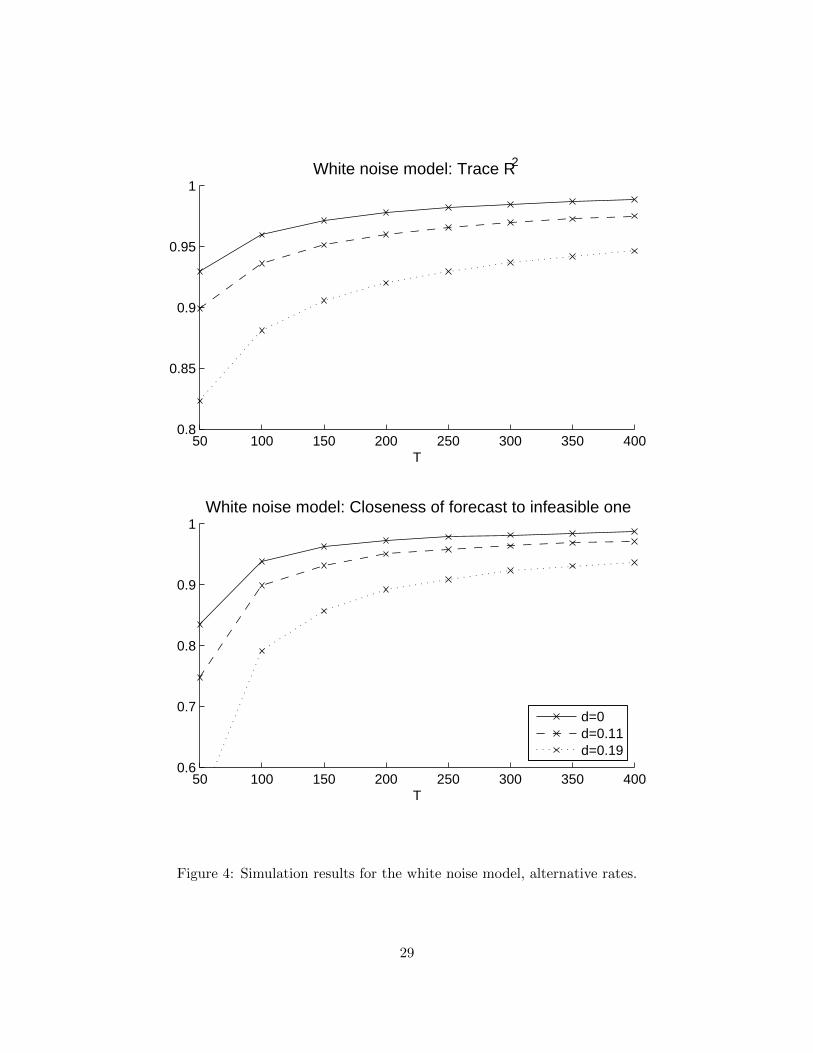
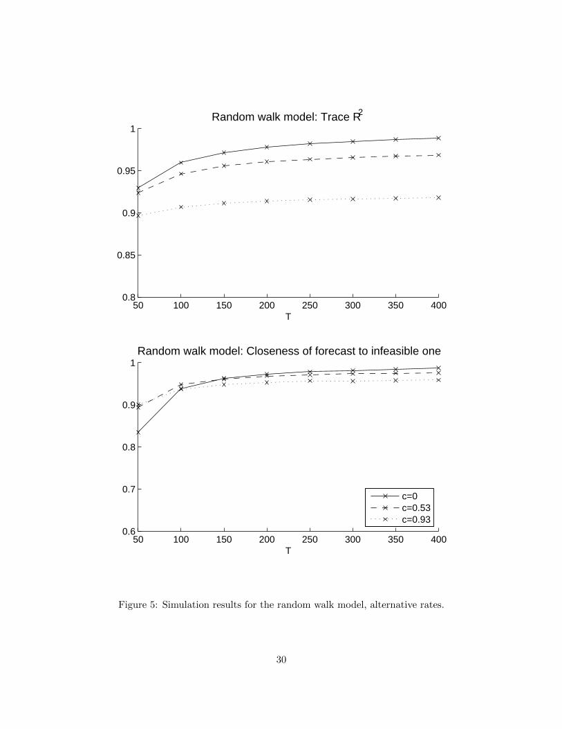
We now turn to the more detailed asymptotic rates stated in Theorem 1. Our method of proofand the calculations in Section 3.2 suggest that it may not in general be possible to improve uponthe RNT rate for our three examples of break processes. To investigate this claim, we carry outtwo exercises. First, we set N = T and execute a separate set of simulations in which λitp− λi0p =dT 1/4ξitp for the white noise model, λitp − λi,t−1,p = cT−1/2ζitp for the random walk model, andthe number of shifting series in the large break model is set to [bN ]. These three rates all (just)violate the conditions for mean square consistency in Theorem 1. To make the results comparableto Figures 2–3, we scale down our choices of b, c and d so that the amount of time variationin the two experiments coincide for T = 200. All other parameters are unchanged. See Figures4–6 for the results. As hypothesized, for the random walk and large break models the trace R2

curve flattens out for large T , instead of converging with the no-instability curve as in Figures 2–3.For the white noise model, convergence seems to still obtain with hNT = dT 1/4.19 It would beinteresting to explore whether temporal or cross-sectional dependence in the disturbances ξit wouldmake Theorem 1 tight also for the white noise model.

Second, we construct a “rate frontier” that corresponds to the predictions of Theorem 1 for thespecial case of the random walk model, which is the break process that has received most attentionin the literature. Consider the explicit rate expression (5)–(6) for the random walk model under theassumptions N = [Tµ] and hNT = cT−γ . In the following we set µ = 1 so that the rate exponent(6) reduces to

m(γ) = m(1, γ) = max−1, 2− 4γ.

The flat profile of the trace R2 statistic in Figure 5 is fully consistent with m(1/2) = 0. Thesecalculations pertain to the worst-case rate stated in Theorem 1. While Section 3.2 showed suggestivecalculations for the special case Λ0 = 0, we have not been able to prove that the convergence rateRNT is sharp, in the sense that a generic DFM with random walk factor loadings that satisfiesAssumptions 1–5 achieves the RNT rate. Instead, we provide simulation evidence indicating thatthe independent random walk model achieves the stated bound. We maintain the simulationdesign described in Section 5.1 with a = β = ρ = 0 and N = T , except that we set hNT = 5T−γ

and vary γ over the range 0.25, 0.30, 0.35, . . . , 1.50. For each value of γ and each sample sizeT = 200, 300, . . . , 700 we compute the statistic

MSE (γ, T ) = T−1(E‖F‖2 − E‖PF F‖2),

where E denotes the average over 500 Monte Carlo repetitions. This statistic is a close analog ofthe mean square error that is the object of study in Theorem 1. Our theoretical results suggest

19This is consistent with the calculations in Section 3.2, which showed that hNT = o(T 1/2) is necessary and sufficientfor mean square consistency when Λ0 = 0, Ft ≡ 1, k = r = 1 and T/N → θ ∈ (0,∞), cf. equation (7).

18

that MSE (γ, T ) should grow or decay at rate Tm(γ). We verify this by regressing, for each γ,

log MSE (γ, T ) = constantγ +mγ log T,

using our six observations T = 200, . . . , 700. Figure 7 plots the estimates mγ against γ alongwith the theoretical values m(γ). The estimated rate frontier is strikingly close to the theoreticalone, although some finite-sample issues remain for intermediate values of γ. This corroborates ourconjecture that Theorem 1 provides sharp rates for the independent random walk case.

6 Discussion and conclusions

The theoretical results of Section 3 and the simulation study of Section 5 point towards a consid-erable amount of robustness of the principal components estimator of the factors when the factorloading matrix varies over time. Although we have not proved that the consistency rate functionpresented in Section 3.1 is tight in a formal sense, inspection of our proof, as well as calculationsfor special cases and Monte Carlo evidence, do not suggest any room for improvement, particularlyfor the random walk and large break models. In this sense our rate function represents an upperbound on the parameter instability that can be tolerated by the principal components estima-tor. The amount of such instability is quite large when calibrated to values of N and T typicallyused in applied work, which is reassuring for the nascent empirical research agenda that allows forstructural instability in estimation of DFMs (Eickmeier et al., 2011; Korobilis, forthcoming).

Our evidence concerning the robustness of the principal components estimator raises a tensionwith the results in Breitung and Eickmeier (2011), who stress the harmful effect of undetectedfactor loading breaks on rank estimation. Our simulations show that diffusion index forecastingusing principal components estimates can be effective even when the rank of the factor space is notestimated consistently. Indeed, we conjecture (but do not prove) that the principal componentsestimator and feasible diffusion index regression will be consistent under sequences of breaks forwhich the Breitung and Eickmeier (2011) test rejects. Furthermore, our simulations indicate thatthe direction of the rank estimation bias depends on the type of structural instability. Sortingout the relative importance of these countervailing forces for the sampling distribution of forecastswould be of independent interest and would also return the large-dimensional discussion here tothe bias-variance tradeoffs associated with ignoring breaks tackled in a low-dimensional setting byPesaran and Timmermann (2005, 2007).

In some applications, such as with data on asset returns, accurate estimation of the number offactors is of direct concern. Our results suggest that the allowable amount of structural instabilityin these cases is smaller than for forecasting purposes. More work is needed to establish necessaryconditions for consistent rank estimation, and if necessary, to develop rank estimators that aremore robust to different types of instability.

19

A Appendix

A.1 Proof of Theorem 1

To lighten the notation, we denote∑

i =∑N

i=1 (the same for j) and∑

s =∑T

s=1 (the same for t).

A double sum∑N

i=1

∑Nj=1 is denoted

∑i,j .

Proof of Theorem 1. We extend the proof of Theorem 1 in Bai and Ng (2002). By the definitionof the estimator F k, we have F k = (NT )−1XX ′F k, where F k

′F k/T = Ik (Bai and Ng, 2008).

Define e = (e1, . . . , eT )′ and w = (w1, . . . , wT )′. Since

XX ′ = FΛ′0Λ0F′ + FΛ′0(e+ w)′ + (e+ w)Λ0F

′ + (e+ w)(e+ w)′,

we can write

F kt −Hk′Ft = (NT )−1F k′FΛ′0et + F k

′eΛ0Ft + F k

′eet + F k

′FΛ′0wt

+ F k′wΛ0Ft + F k

′wwt + F k

′ewt + F k

′wet

.

Label the eight terms on the right-hand side A1t, . . . , A8t, respectively. By Loeve’s inequality,

T−1∑t

‖F kt −Hk′Ft‖2 ≤ 8

8∑n=1

(T−1

∑t

‖Ant‖2). (13)

Bai and Ng (2002) have shown that the terms corresponding to n = 1, 2, 3 are Op(C−2NT ) under

Assumptions 1–3. We proceed to bound the remaining terms in probability.We have

‖A4t‖2 ≤

(T−1

∑s

‖F ks ‖2)(

T−1∑s

‖Fs‖2)∥∥N−1Λ′0wt

∥∥2.

The first factor equals tr(F k′F k/T ) = tr(Ik) = k. The second factor is Op(1) by Assumption 1.

Also,

E

∥∥∥∥Λ′0wtN

∥∥∥∥2

≤ N−2∑i,j

|E(witwjt)λ′i0λj0|

≤ λ2h2NTN

−2∑i,j

|E(ξitFtξitFt)|

≤ r2λ2 supp,q

h2NTN

−2∑i,j

|E(ξitpFtpξitqFtq)|

= O(h2NTN

−2Q1(N,T )),

uniformly in t, by Assumption 4.1. Hence,

T−1∑t

‖A4t‖2 = Op(h2NTN

−2Q1(N,T )).

Similarly,

‖A5t‖2 ≤

(T−1

∑s

‖F ks ‖2)(

(N2T )−1∑s

(w′sΛ0Ft)2

),

20

where the first term is O(1) and

(N2T )−1E∑s

(w′sΛ0Ft)2 ≤ (N2T )−1

∑s

∑i,j

|E(wiswjsλ′i0Ftλ

′j0Ft)|

≤ r4λ2 supp1,q1,p2,q2

h2NT (N2T )−1

∑s

∑i,j

|E(ξisp1ξjsq1Fsp1Fsq1Ftp2Ftq2)|.

By summing over t, dividing by T and using Assumption 4.2 we obtain

T−1∑t

‖A5t‖2 = Op(h2NTN

−2T−2Q2(N,T )).

For the sixth term,

E‖A6t‖2 ≤ E

(T−1

∑s

‖F ks ‖2)(

(N2T )−1∑s

(w′swt)2

)= k(N2T )−1

∑s

∑i,j

E(wiswitwjswjt)

≤ kr4 supp1,q1,p2,q2

h4NT

N2T

∑s

∑i,j

|E(ξisp1ξjsq1ξitp2ξjtq2Fsp1Fsq1Ftp2Ftq2)|.

By Assumption 4.3, it follows that

T−1∑t

‖A6t‖2 = Op(h4NTN

−2T−2Q3(N,T )).

Regarding the seventh term, using Assumption 5,

E‖A7t‖2 ≤ E

(T−1

∑s

‖F ks ‖2)(

(N2T )−1∑s

(e′swt)2

)= k(N2T )−1

∑s

∑i,j

E(eisejs)E(witwjt)

≤ k(N2T )−1∑s

∑i,j

(E(e2is)E(e2

js))1/2|E(witwjt)|

≤ kr2M supp,q

h2NT (N2T )−1

∑s

∑i,j

|E(ξitpξjtqFtpFtq)|

= O(h2NTN

−2Q1(N,T )),

uniformly in t. The second-to-last line uses E(e2it) ≤M , whereas the last follows from Assumption

4.1. We conclude thatT−1

∑t

‖A7t‖2 = Op(h2NTN

−2Q1(N,T )).

A similar argument gives

T−1∑t

‖A8t‖2 = Op(h2NTN

−2Q1(N,T )).

We conclude that the right-hand side of inequality (13) is the sum of variables of four stochastic or-ders: Op(C

−2NT ), Op(h

2NTN

−2Q1(N,T )), Op(h2NTN

−2T−2Q2(N,T )) and Op(h4NTN

−2T−2Q3(N,T )).The statement of the theorem follows.

21

A.2 Detailed calculations for the case Λ0 = 0

Using the definitions of F k and Hk, we get

T−1T∑t=1

‖F kt −Hk ′Ft‖2 = tr

(F k − FHk)(F k − FHk)′

= N−2T−3trF k′(XX ′ − FΛ′0Λ0F

′)(XX ′ − FΛ′0Λ0F′)′F k

.

Let Λ0 = 0. By definition, F k equals√T times the T×k matrix whose columns are the eigenvectors

of XX ′ corresponding to its k largest eigenvalues. That is, if we write (XX ′)R = RC, where Ris the orthogonal matrix of eigenvectors and C the diagonal matrix of eigenvalues (in descendingorder), we have

√TR = (F k, F k) for a T × (T − k) matrix F k that satisfies F k′F k = 0. Observe

thatF k =

√TR(Ik, 0k×(T−k))

′,

so(XX ′)F k =

√T (XX ′)R(Ik, 0k×(T−k))

′ =√TRC(Ik, 0k×(T−k))

′,

and

F k′(XX ′)(XX ′)F k = T (Ik, 0k×(T−k))CR′RC(Ik, 0k×(T−k))

′

= TC2k ,

where Ck = (Ik, 0k×(T−k))C(Ik, 0k×(T−k))′ denotes the diagonal matrix containing the k largest

eigenvalues ω1, . . . , ωk of XX ′. Hence,

T−1T∑t=1

‖F kt −Hk ′Ft‖2 = (NT )−2trC2k

= (NT )−2k∑l=1

ω2l .

(14)

Example 1 (white noise, continued). Under the assumptions in the main text, the T × Ndata matrix X has elements xit = eit + hNT ξit that are i.i.d. across i and t with mean 0 andvariance ΩNT = σ2

e + h2NTσ

2ξ . Let Z be a T ×N matrix with elements zit = xit/

√ΩNT . Then zit is

i.i.d. across i and t with mean zero and unit variance. Let ω1 denote the largest eigenvalue of thesample covariance matrix N−1ZZ ′. By Theorem 5.8 of Bai and Silverstein (2009), ω1

a.s.→ (1+√θ)2.

Because the largest eigenvalue of N−1XX ′ satisfies ω1 = ΩNT ω1, the result (7) follows from (14).

22

Example 2 (random walk, continued). Let 1T denote the T -vector of ones. Setting k = 1 inequation (14), we obtain

T−1T∑t=1

‖F kt −Hk ′Ft‖2 = (NT )−2

(maxv∈RT

v′XX ′v

v′v

)2

≥ (NT )−2

(1′TXX

′1TT

)2

=1

N2T 4

N∑i=1

(T∑t=1

xit

)22

.

Jensen’s inequality and cross-sectional i.i.d.-ness of xit implies

E

N∑i=1

(T∑t=1

xit

)22

≥

NE( T∑t=1

xit

)22

,

so inequality (8) follows.

Example 3 (single large break, continued). In the large break model, wit = ∆iFt1t≥κ+1.Denote the last (T − κ) elements of the T -vector F by Fκ+1:T . Then we can write

w = (w1, . . . , wT )′ = hNT

(0κ×N

Fκ+1:T ⊗∆′

),

so that

ww′ = h2NT

(0κ×κ 0κ×(T−κ)

0(T−κ)×κ (Fκ+1:TF′κ+1:T )‖∆‖2

).

It follows that the eigenvalues of ww′ are 0 (with multiplicity κ) along with h2NT ‖∆‖2 times the

(T − κ) eigenvalues of Fκ+1:TF′κ+1:T . But the eigenvalues of Fκ+1:TF

′κ+1:T are just ‖Fκ+1:T ‖2

(with multiplicity 1) and 0 (with multiplicity T − κ − 1). The k largest eigenvalues ω1, . . . , ωk ofXX ′ = ww′ are therefore

ω1 = h2NT ‖∆‖2‖Fκ+1:T ‖2, ω2 = ω3 = · · · = ωk = 0.

Consequently, regardless of the number of estimated factors k,

T−1T∑t=1

‖F kt −Hk ′Ft‖2 = (NT )−2k∑l=1

ω2l

=h4NT

(NT )2‖∆‖4‖Fκ+1:T ‖4

=h4NT

N2‖∆‖4(1− τ)2

(1

T − κ

T∑t=κ+1

F 2t + op(1)

)2

where the last equality uses T − κ = (1− τ)T (1 + o(1)). Expression (9) follows.

23

A.3 Comparison of our Monte Carlo calibration with Eickmeier et al. (2011)

Eickmeier et al. (2011) use a two-step maximum likelihood procedure to estimate a five-factorDFM with time-varying parameters on quarterly U.S. data from 1972 to 2007. As in some of oursimulations, the factor loadings in their model evolve as independent random walks. From theirsmoothed estimates of the factor loading paths (restricting attention to the paths that exhibitnon-negligible time variation) one obtains a median standard deviation of the innovations equal to0.0165 for loadings on the first factor, which has the largest median loading innovation standarddeviation of the five factors. Because their sample size is T = 140, the random walk specificationimplies a median standard deviation of λiT1−λi01 of about 0.20; the 95th percentile of the impliedstandard deviation of λiT1 − λi01 is about 0.75. The 5–95 percentile range of estimated initialfactor loadings is [−0.87, 0.28].20 As explained in the main text, in our random walk design witha = β = ρ = 0, c = 2 and T = 200, the standard deviation of λiT1 − λi01 is 0.53 for all i, while the5–95 percentile range for initial factor loadings is [−0.74, 0.74]. Our c = 2 calibration is thereforesimilar to the Eickmeier et al. (2011) estimated amount of factor loading time variation in U.S.data, while our c = 3.5 simulations appear to exhibit substantially more instability.

References

Amengual, D. and Watson, M. W. (2007), ‘Consistent Estimation of the Number of Dynamic Factors in aLarge N and T Panel’, Journal of Business and Economic Statistics 25(1), 91–96.

Bai, J. and Ng, S. (2002), ‘Determining the Number of Factors in Approximate Factor Models’, Econometrica70(1), 191–221.

Bai, J. and Ng, S. (2006a), ‘Confidence Intervals for Diffusion Index Forecasts and Inference for Factor-Augmented Regressions’, Econometrica 74(4), 1133–1150.

Bai, J. and Ng, S. (2006b), ‘Determining the number of factors in approximate factor models, Errata’.Manuscript, Columbia University.

Bai, J. and Ng, S. (2008), ‘Large Dimensional Factor Analysis’, Foundations and Trends in Econometrics3(2), 89–163.

Bai, Z. and Silverstein, J. (2009), Spectral Analysis of Large Dimensional Random Matrices, Springer Seriesin Statistics, Springer.

Banerjee, A., Marcellino, M. and Masten, I. (2008), Forecasting Macroeconomic Variables Using DiffusionIndexes in Short Samples with Structural Change, in D. E. Rapach and M. E. Wohar, eds, ‘Forecastingin the Presence of Structural Breaks and Model Uncertainty (Frontiers of Economics and Globalization,Volume 3)’, Emerald Group Publishing Limited, chapter 4, pp. 149–194.

Breitung, J. and Eickmeier, S. (2011), ‘Testing for structural breaks in dynamic factor models’, Journal ofEconometrics 163(1), 71–84.

Chudik, A. and Pesaran, M. H. (2011), ‘Infinite-dimensional VARs and factor models’, Journal of Econo-metrics 163(1), 4–22.

Clements, M. and Hendry, D. (1998), Forecasting Economic Time Series, Cambridge University Press.

20We are grateful to Wolfgang Lemke and Massimiliano Marcellino for helping us obtain these figures.

24

Eickmeier, S., Lemke, W. and Marcellino, M. (2011), ‘Classical time-varying FAVAR models – estimation,forecasting and structural analysis’. Deutsche Bundesbank Discussion Paper, No. 04/2011.

Eickmeier, S. and Ziegler, C. (2008), ‘How Successful are Dynamic Factor Models at Forecasting Output andInflation? A Meta-Analytic Approach’, Journal of Forecasting 27(3), 237–265.

Engle, R. and Watson, M. W. (1981), ‘A One-Factor Multivariate Time Series Model of Metropolitan WageRates’, Journal of the American Statistical Association 76(376), 774–781.

Forni, M., Hallin, M., Lippi, M. and Reichlin, L. (2000), ‘The Generalized Dynamic-Factor Model: Identifi-cation and Estimation’, Review of Economics and Statistics 82(4), 540–554.

Geweke, J. (1977), The Dynamic Factor Analysis of Economic Time Series, in D. J. Aigner and A. S.Goldberger, eds, ‘Latent Variables in Socio-Economic Models’, North-Holland.

Hamilton, J. (1989), ‘A New Approach to the Economic Analysis of Nonstationary Time Series and theBusiness Cycle’, Econometrica 57(2), 357–384.

Korobilis, D. (forthcoming), ‘Assessing the Transmission of Monetary Policy Using Time-varying ParameterDynamic Factor Models’, Oxford Bulletin of Economics and Statistics .

Pesaran, H. M., Pettenuzzo, D. and Timmermann, A. (2006), ‘Forecasting Time Series Subject to MultipleStructural Breaks’, Review of Economic Studies 73(4), 1057–1084.

Pesaran, M. H. and Timmermann, A. (2005), ‘Small sample properties of forecasts from autoregressivemodels under structural breaks’, Journal of Econometrics 129(1-2), 183–217.

Pesaran, M. H. and Timmermann, A. (2007), ‘Selection of estimation window in the presence of breaks’,Journal of Econometrics 137(1), 134–161.

Sargent, T. (1989), ‘Two Models of Measurements and the Investment Accelerator’, The Journal of PoliticalEconomy 97(2), 251–287.

Sargent, T. and Sims, C. A. (1977), Business Cycle Modeling Without Pretending to Have Too Much APriori Economic Theory, in C. A. Sims, ed., ‘New Methods in Business Research’, Federal Reserve Bankof Minneapolis.

Stock, J. H. and Watson, M. W. (1989), New Indexes of Coincident and Leading Economic Indicators, in O. J.Blanchard and S. Fischer, eds, ‘NBER Macroeconomics Annual 1989’, Vol. 4, MIT Press, pp. 351–409.

Stock, J. H. and Watson, M. W. (1998a), ‘Diffusion Indexes’. NBER Working Paper 6702.

Stock, J. H. and Watson, M. W. (1998b), ‘Median Unbiased Estimation of Coefficient Variance in a Time-Varying Parameter Model’, Journal of the American Statistical Association 93(441), 349–358.

Stock, J. H. and Watson, M. W. (2002), ‘Forecasting Using Principal Components From a Large Number ofPredictors’, Journal of the American Statistical Association 97(460), 1167–1179.

Stock, J. H. and Watson, M. W. (2009), Forecasting in Dynamic Factor Models Subject to Structural Insta-bility, in D. F. Hendry, J. Castle and N. Shephard, eds, ‘The Methodology and Practice of Econometrics:A Festschrift in Honour of David F. Hendry’, Oxford University Press, pp. 173–205.

Stock, J. H. and Watson, M. W. (2011), Dynamic Factor Models, in M. P. Clement and D. F. Hendry, eds,‘The Oxford Handbook of Economic Forecasting’, Oxford University Press, pp. 35–59.

Watson, M. W. and Engle, R. F. (1983), ‘Alternative Algorithms for the Estimation of Dynamic Factor,MIMIC and Varying Coefficient Regression Models’, Journal of Econometrics 23(3), 385–400.

25

50 100 150 200 250 300 350 4000.8

0.85

0.9

0.95

1White noise model: Trace R2

T

50 100 150 200 250 300 350 4000.6

0.7

0.8

0.9

1White noise model: Closeness of forecast to infeasible one

T

d=0d=0.4d=0.7

Figure 1: Simulation results for the white noise model, benchmark parameter and rate choices.Actual observations are marked with “x.” Each is based on 5,000 Monte Carlo repetitions. Thelines are piecewise linear interpolations.

26

50 100 150 200 250 300 350 4000.8

0.85

0.9

0.95

1Random walk model: Trace R2

T

50 100 150 200 250 300 350 4000.6

0.7

0.8

0.9

1Random walk model: Closeness of forecast to infeasible one

T

c=0c=2c=3.5

Figure 2: Simulation results for the random walk model, benchmark parameter and rate choices.

27

50 100 150 200 250 300 350 4000.8

0.85

0.9

0.95

1Large break model: Trace R2

T

50 100 150 200 250 300 350 4000.6

0.7

0.8

0.9

1Large break model: Closeness of forecast to infeasible one

T

b=0b=3.5b=7

Figure 3: Simulation results for the large break model, benchmark parameter and rate choices.

28

50 100 150 200 250 300 350 4000.8

0.85

0.9

0.95

1White noise model: Trace R2

T

50 100 150 200 250 300 350 4000.6

0.7

0.8

0.9

1White noise model: Closeness of forecast to infeasible one

T

d=0d=0.11d=0.19

Figure 4: Simulation results for the white noise model, alternative rates.

29

50 100 150 200 250 300 350 4000.8

0.85

0.9

0.95

1Random walk model: Trace R2

T

50 100 150 200 250 300 350 4000.6

0.7

0.8

0.9

1Random walk model: Closeness of forecast to infeasible one

T

c=0c=0.53c=0.93

Figure 5: Simulation results for the random walk model, alternative rates.

30

50 100 150 200 250 300 350 4000.8

0.85

0.9

0.95

1Large break model: Trace R2

T

50 100 150 200 250 300 350 4000.6

0.7

0.8

0.9

1Large break model: Closeness of forecast to infeasible one

T

b=0b=0.25b=0.50

Figure 6: Simulation results for the large break model, alternative rates.

31

0.25 0.5 0.75 1 1.25 1.5−2

−1.5

−1

−0.5

0

0.5

1Finite−sample and theoretical rate frontiers

γ

m

Finite−sampleTheoretical

Figure 7: Rate frontiers for the random walk model with c = 5, N = T and hNT = cT−γ . The solidline interpolates between the finite-sample rate exponent estimates mγ (observations are markedwith “x”), while the dotted line represents the theoretical rate exponent m(γ).

32

Monte Carlo simulations: White noise modeld = 0 d = 0.4 d = 0.7

k = r IC k = r IC k = r IC

T N R2F ,F

S2y,y R2

F ,FS2y,y E(k) R2

F ,FS2y,y R2

F ,FS2y,y E(k) R2

F ,FS2y,y R2

F ,FS2y,y E(k)

a = 0, β = 0, ρ = 0

50 50 0.93 0.83 0.94 0.50 3.4 0.86 0.64 0.91 −0.83 1.6 0.71 0.25 0.84 −2.77 1.050 100 0.96 0.93 0.96 0.88 4.7 0.92 0.84 0.94 0.35 2.9 0.81 0.59 0.89 −1.72 1.1

100 100 0.96 0.94 0.96 0.93 5.0 0.93 0.88 0.93 0.66 3.9 0.84 0.70 0.90 −1.88 1.3100 200 0.98 0.97 0.98 0.97 5.0 0.96 0.94 0.96 0.93 5.0 0.91 0.86 0.93 0.13 2.7200 100 0.96 0.94 0.96 0.94 5.0 0.93 0.89 0.93 0.86 4.8 0.86 0.77 0.88 −0.20 2.4200 200 0.98 0.97 0.98 0.97 5.0 0.96 0.95 0.96 0.95 5.0 0.92 0.90 0.93 0.70 4.1200 400 0.99 0.99 0.99 0.99 5.0 0.98 0.97 0.98 0.97 5.0 0.96 0.95 0.96 0.94 5.0

a = 0.5, β = 0, ρ = 0

50 50 0.91 0.77 0.93 0.53 3.7 0.86 0.64 0.91 −0.42 2.0 0.75 0.38 0.86 −2.39 1.150 100 0.95 0.90 0.95 0.88 4.8 0.92 0.84 0.93 0.57 3.6 0.84 0.68 0.91 −1.01 1.4

100 100 0.96 0.93 0.96 0.92 5.0 0.93 0.89 0.93 0.78 4.4 0.87 0.77 0.91 −0.70 1.9100 200 0.98 0.97 0.98 0.97 5.0 0.96 0.95 0.96 0.94 5.0 0.93 0.89 0.93 0.65 3.8200 100 0.96 0.94 0.96 0.94 5.0 0.93 0.90 0.93 0.90 4.9 0.88 0.82 0.89 0.41 3.4200 200 0.98 0.97 0.98 0.97 5.0 0.96 0.95 0.96 0.95 5.0 0.93 0.92 0.94 0.87 4.8200 400 0.99 0.99 0.99 0.99 5.0 0.98 0.98 0.98 0.98 5.0 0.96 0.96 0.96 0.96 5.0

a = 0, β = 0.5, ρ = 0

50 50 0.91 0.76 0.93 0.53 3.7 0.85 0.58 0.90 −0.87 1.7 0.70 0.22 0.83 −3.09 1.050 100 0.95 0.91 0.96 0.87 4.7 0.92 0.83 0.93 0.39 3.0 0.80 0.57 0.89 −1.58 1.1

100 100 0.96 0.92 0.96 0.92 5.0 0.92 0.87 0.93 0.66 4.0 0.84 0.70 0.89 −1.90 1.3100 200 0.98 0.97 0.98 0.97 5.0 0.96 0.94 0.96 0.93 5.0 0.91 0.86 0.93 0.15 2.7200 100 0.96 0.94 0.95 0.94 5.0 0.92 0.88 0.92 0.86 4.8 0.85 0.76 0.88 −0.19 2.4200 200 0.98 0.97 0.98 0.97 5.0 0.96 0.95 0.96 0.95 5.0 0.92 0.90 0.92 0.70 4.1200 400 0.99 0.99 0.99 0.99 5.0 0.98 0.97 0.98 0.97 5.0 0.96 0.95 0.96 0.94 5.0

a = 0, β = 0, ρ = 0.9

50 50 0.95 0.81 0.97 0.43 2.3 0.61 0.03 0.84 −1.18 1.0 0.32 −0.96 0.52 −2.94 1.050 100 0.97 0.91 0.98 0.69 2.9 0.70 0.37 0.91 −0.75 1.0 0.38 −0.38 0.67 −1.74 1.0

100 100 0.97 0.94 0.97 0.81 3.9 0.75 0.43 0.89 −1.46 1.0 0.39 −0.43 0.67 −2.48 1.0100 200 0.98 0.97 0.98 0.94 4.6 0.84 0.65 0.94 −0.75 1.3 0.48 −0.00 0.80 −1.60 1.0200 100 0.97 0.94 0.97 0.93 4.9 0.79 0.55 0.88 −1.68 1.2 0.43 −0.50 0.68 −3.19 1.0200 200 0.98 0.97 0.98 0.97 5.0 0.88 0.80 0.93 −0.52 1.7 0.57 0.11 0.81 −2.02 1.0200 400 0.99 0.99 0.99 0.99 5.0 0.94 0.90 0.95 0.40 2.7 0.69 0.45 0.88 −1.99 1.0

a = 0.5, β = 0.5, ρ = 0.9

50 50 0.94 0.74 0.95 0.65 3.7 0.71 0.24 0.88 −1.05 1.0 0.41 −0.55 0.66 −1.91 1.050 100 0.97 0.86 0.97 0.83 4.5 0.80 0.51 0.93 −0.52 1.2 0.49 −0.09 0.79 −1.40 1.0

100 100 0.96 0.90 0.97 0.88 4.6 0.82 0.56 0.92 −1.05 1.3 0.50 −0.07 0.77 −2.04 1.0100 200 0.98 0.96 0.98 0.95 4.9 0.90 0.76 0.95 −0.07 1.9 0.61 0.25 0.87 −1.51 1.0200 100 0.96 0.93 0.96 0.92 5.0 0.84 0.66 0.90 −0.66 1.8 0.55 −0.07 0.76 −2.91 1.0200 200 0.98 0.97 0.98 0.96 5.0 0.91 0.85 0.94 0.19 2.5 0.70 0.39 0.86 −1.93 1.0200 400 0.99 0.98 0.99 0.98 5.0 0.95 0.93 0.96 0.71 3.6 0.80 0.64 0.92 −1.79 1.0

Table 1: Simulation results for DGPs with white noise disturbances in the factor loadings.

33

Monte Carlo simulations: Random walk modelc = 0 c = 2 c = 3.5

k = r IC k = r IC k = r IC

T N R2F ,F

S2y,y R2

F ,FS2y,y E(k) R2

F ,FS2y,y R2

F ,FS2y,y E(k) R2

F ,FS2y,y R2

F ,FS2y,y E(k)

a = 0, β = 0, ρ = 0

50 50 0.93 0.83 0.94 0.50 3.4 0.91 0.90 0.91 0.89 4.8 0.87 0.89 0.87 0.90 5.250 100 0.96 0.93 0.96 0.88 4.7 0.93 0.93 0.93 0.93 5.0 0.89 0.92 0.88 0.91 5.7

100 100 0.96 0.94 0.96 0.93 5.0 0.94 0.94 0.94 0.95 5.0 0.89 0.94 0.89 0.94 5.4100 200 0.98 0.97 0.98 0.97 5.0 0.95 0.96 0.95 0.96 5.0 0.90 0.94 0.89 0.94 6.8200 100 0.96 0.94 0.96 0.94 5.0 0.94 0.95 0.94 0.95 5.0 0.90 0.94 0.90 0.94 5.6200 200 0.98 0.97 0.98 0.97 5.0 0.96 0.97 0.96 0.97 5.0 0.91 0.95 0.91 0.95 7.0200 400 0.99 0.99 0.99 0.99 5.0 0.97 0.98 0.97 0.97 5.0 0.92 0.96 0.91 0.96 9.5

a = 0.5, β = 0, ρ = 0

50 50 0.91 0.77 0.93 0.53 3.7 0.91 0.90 0.91 0.87 4.7 0.88 0.89 0.88 0.90 5.150 100 0.95 0.90 0.95 0.88 4.8 0.94 0.94 0.94 0.94 5.0 0.90 0.92 0.89 0.92 5.5

100 100 0.96 0.93 0.96 0.92 5.0 0.94 0.95 0.94 0.95 5.0 0.90 0.94 0.90 0.94 5.2100 200 0.98 0.97 0.98 0.97 5.0 0.96 0.96 0.96 0.96 5.0 0.91 0.95 0.91 0.94 6.1200 100 0.96 0.94 0.96 0.94 5.0 0.95 0.95 0.95 0.95 5.0 0.92 0.95 0.91 0.95 5.2200 200 0.98 0.97 0.98 0.97 5.0 0.97 0.97 0.97 0.97 5.0 0.93 0.96 0.92 0.96 5.8200 400 0.99 0.99 0.99 0.99 5.0 0.98 0.98 0.98 0.98 5.0 0.93 0.96 0.93 0.96 8.4

a = 0, β = 0.5, ρ = 0

50 50 0.91 0.76 0.93 0.53 3.7 0.91 0.89 0.91 0.89 4.8 0.87 0.89 0.87 0.90 5.350 100 0.95 0.91 0.96 0.87 4.7 0.93 0.93 0.93 0.93 5.0 0.89 0.92 0.88 0.91 5.8

100 100 0.96 0.92 0.96 0.92 5.0 0.94 0.94 0.94 0.95 5.0 0.89 0.94 0.89 0.94 5.5100 200 0.98 0.97 0.98 0.97 5.0 0.95 0.96 0.95 0.96 5.0 0.90 0.94 0.89 0.94 6.9200 100 0.96 0.94 0.95 0.94 5.0 0.94 0.95 0.94 0.95 5.0 0.90 0.95 0.90 0.94 5.8200 200 0.98 0.97 0.98 0.97 5.0 0.96 0.97 0.96 0.97 5.0 0.91 0.95 0.91 0.95 7.1200 400 0.99 0.99 0.99 0.99 5.0 0.97 0.98 0.97 0.98 5.0 0.92 0.96 0.91 0.96 9.5

a = 0, β = 0, ρ = 0.9

50 50 0.95 0.81 0.97 0.43 2.3 0.94 0.90 0.94 0.91 5.5 0.94 0.90 0.94 0.92 7.350 100 0.97 0.91 0.98 0.69 2.9 0.95 0.92 0.95 0.94 6.4 0.94 0.92 0.94 0.94 8.6

100 100 0.97 0.94 0.97 0.81 3.9 0.93 0.93 0.92 0.95 6.7 0.91 0.93 0.91 0.95 9.2100 200 0.98 0.97 0.98 0.94 4.6 0.93 0.94 0.93 0.97 7.8 0.92 0.94 0.91 0.96 9.9200 100 0.97 0.94 0.97 0.93 4.9 0.91 0.94 0.90 0.95 7.4 0.88 0.94 0.88 0.96 9.9200 200 0.98 0.97 0.98 0.97 5.0 0.92 0.95 0.91 0.97 8.3 0.89 0.95 0.88 0.97 10.0200 400 0.99 0.99 0.99 0.99 5.0 0.92 0.95 0.91 0.98 9.6 0.89 0.95 0.88 0.97 10.0

a = 0.5, β = 0.5, ρ = 0.9

50 50 0.94 0.74 0.95 0.65 3.7 0.94 0.90 0.94 0.91 6.8 0.94 0.90 0.94 0.92 8.350 100 0.97 0.86 0.97 0.83 4.5 0.95 0.92 0.95 0.95 8.4 0.94 0.92 0.94 0.94 9.7

100 100 0.96 0.90 0.97 0.88 4.6 0.93 0.93 0.92 0.95 7.7 0.92 0.93 0.91 0.95 9.7100 200 0.98 0.96 0.98 0.95 4.9 0.94 0.95 0.93 0.97 9.2 0.92 0.94 0.91 0.97 10.0200 100 0.96 0.93 0.96 0.92 5.0 0.92 0.94 0.91 0.95 8.0 0.89 0.94 0.88 0.95 10.0200 200 0.98 0.97 0.98 0.96 5.0 0.93 0.95 0.92 0.97 8.9 0.89 0.95 0.89 0.97 10.0200 400 0.99 0.98 0.99 0.98 5.0 0.93 0.96 0.92 0.98 9.9 0.90 0.95 0.89 0.98 10.0

Table 2: Simulation results for DGPs with random walk factor loadings.

34

Monte Carlo simulations: Large break modelb = 0 b = 3.5 b = 7

k = r IC k = r IC k = r IC

T N R2F ,F

S2y,y R2

F ,FS2y,y E(k) R2

F ,FS2y,y R2

F ,FS2y,y E(k) R2

F ,FS2y,y R2

F ,FS2y,y E(k)

a = 0, β = 0, ρ = 0

50 50 0.93 0.83 0.94 0.50 3.4 0.90 0.83 0.90 0.59 3.6 0.83 0.82 0.84 0.58 3.750 100 0.96 0.93 0.96 0.88 4.7 0.94 0.92 0.94 0.89 4.7 0.89 0.91 0.89 0.89 4.8

100 100 0.96 0.94 0.96 0.93 5.0 0.94 0.94 0.94 0.93 5.0 0.88 0.93 0.88 0.93 5.1100 200 0.98 0.97 0.98 0.97 5.0 0.97 0.97 0.96 0.97 5.1 0.93 0.96 0.93 0.97 5.3200 100 0.96 0.94 0.96 0.94 5.0 0.93 0.94 0.93 0.94 5.2 0.87 0.94 0.87 0.94 5.5200 200 0.98 0.97 0.98 0.97 5.0 0.96 0.97 0.96 0.97 5.2 0.93 0.97 0.92 0.97 5.6200 400 0.99 0.99 0.99 0.99 5.0 0.98 0.98 0.98 0.99 5.2 0.96 0.98 0.95 0.99 5.6

a = 0.5, β = 0, ρ = 0

50 50 0.91 0.77 0.93 0.53 3.7 0.88 0.79 0.89 0.61 3.8 0.82 0.79 0.83 0.62 3.950 100 0.95 0.90 0.95 0.88 4.8 0.93 0.90 0.93 0.89 4.9 0.88 0.89 0.88 0.88 5.0

100 100 0.96 0.93 0.96 0.92 5.0 0.93 0.93 0.93 0.93 5.0 0.88 0.93 0.88 0.93 5.2100 200 0.98 0.97 0.98 0.97 5.0 0.96 0.97 0.96 0.97 5.1 0.93 0.96 0.92 0.97 5.4200 100 0.96 0.94 0.96 0.94 5.0 0.93 0.94 0.93 0.94 5.2 0.87 0.94 0.87 0.94 5.5200 200 0.98 0.97 0.98 0.97 5.0 0.96 0.97 0.96 0.97 5.2 0.93 0.97 0.92 0.97 5.6200 400 0.99 0.99 0.99 0.99 5.0 0.98 0.98 0.98 0.98 5.2 0.96 0.98 0.95 0.98 5.6

a = 0, β = 0.5, ρ = 0

50 50 0.91 0.76 0.93 0.53 3.7 0.87 0.77 0.88 0.61 3.9 0.80 0.77 0.81 0.61 4.150 100 0.95 0.91 0.96 0.87 4.7 0.93 0.90 0.93 0.89 4.8 0.88 0.90 0.88 0.88 5.0

100 100 0.96 0.92 0.96 0.92 5.0 0.93 0.93 0.93 0.93 5.1 0.87 0.92 0.87 0.93 5.3100 200 0.98 0.97 0.98 0.97 5.0 0.96 0.96 0.96 0.96 5.1 0.93 0.96 0.92 0.97 5.4200 100 0.96 0.94 0.95 0.94 5.0 0.93 0.94 0.92 0.94 5.3 0.86 0.93 0.86 0.94 5.7200 200 0.98 0.97 0.98 0.97 5.0 0.96 0.97 0.96 0.97 5.3 0.92 0.97 0.91 0.97 5.7200 400 0.99 0.99 0.99 0.99 5.0 0.98 0.98 0.98 0.98 5.3 0.96 0.98 0.95 0.99 5.7

a = 0, β = 0, ρ = 0.9

50 50 0.95 0.81 0.97 0.43 2.3 0.94 0.81 0.95 0.52 2.4 0.92 0.81 0.93 0.56 2.650 100 0.97 0.91 0.98 0.69 2.9 0.97 0.90 0.97 0.72 3.0 0.95 0.90 0.95 0.73 3.1

100 100 0.97 0.94 0.97 0.81 3.9 0.96 0.93 0.96 0.83 4.0 0.93 0.91 0.93 0.83 4.2100 200 0.98 0.97 0.98 0.94 4.6 0.98 0.97 0.98 0.94 4.7 0.96 0.96 0.96 0.94 4.8200 100 0.97 0.94 0.97 0.93 4.9 0.95 0.94 0.95 0.93 5.0 0.91 0.93 0.91 0.93 5.1200 200 0.98 0.97 0.98 0.97 5.0 0.97 0.97 0.97 0.97 5.1 0.95 0.96 0.94 0.97 5.3200 400 0.99 0.99 0.99 0.99 5.0 0.99 0.98 0.98 0.98 5.1 0.97 0.98 0.97 0.98 5.4

a = 0.5, β = 0.5, ρ = 0.9

50 50 0.94 0.74 0.95 0.65 3.7 0.93 0.75 0.94 0.70 4.1 0.90 0.75 0.91 0.71 4.350 100 0.97 0.86 0.97 0.83 4.5 0.96 0.85 0.96 0.84 4.8 0.94 0.86 0.94 0.85 5.0

100 100 0.96 0.90 0.97 0.88 4.6 0.95 0.89 0.95 0.88 4.8 0.92 0.88 0.92 0.88 5.0100 200 0.98 0.96 0.98 0.95 4.9 0.97 0.95 0.97 0.95 5.2 0.95 0.94 0.95 0.95 5.4200 100 0.96 0.93 0.96 0.92 5.0 0.94 0.92 0.94 0.93 5.3 0.90 0.91 0.90 0.93 5.6200 200 0.98 0.97 0.98 0.96 5.0 0.97 0.96 0.97 0.97 5.3 0.94 0.95 0.94 0.97 5.6200 400 0.99 0.98 0.99 0.98 5.0 0.98 0.98 0.98 0.98 5.3 0.97 0.98 0.96 0.98 5.7

Table 3: Simulation results for DGPs with a single large break in the factor loadings.

35