S1

Supplementary Information

Shape Control in Concave Metal Nanoparticles by Etching

Qiang Li,†

Marcos Rellán-Piñeiro, †

Neyvis Almora-Barrios, †

Miquel Garcia-Ratés, †

Ioannis N.

Remediakis, ‡

and Nuria López*†

†Institute of Chemical Research of Catalonia, ICIQ, The Barcelona Institute of Science and Technology,

Av. Països Catalans, 16, 43007, Tarragona, Spain

‡ Department of Materials Science and Technology, University of Crete, Heraklion, 71003, Greece

Email: nlopez@iciq.es

Electronic Supplementary Material (ESI) for Nanoscale.This journal is © The Royal Society of Chemistry 2017

S2

S1. Pt surfaces

The surface energy 𝛾𝑠, that describes the stability of a surface, is the energy required to cleave a

surface from a bulk crystal. It is given by

𝛾𝑠 =1

2𝐴(𝐸𝑠

𝑢𝑛𝑟𝑒𝑙𝑎𝑥 − 𝑁𝐸𝑏) +1

𝐴(𝐸𝑠

𝑟𝑒𝑙𝑎𝑥 − 𝐸𝑠𝑢𝑛𝑟𝑒𝑙𝑎𝑥) (1)

Here, 𝐴 is the area of the surface considered, 𝐸𝑠𝑟𝑒𝑙𝑎𝑥 and 𝐸𝑠

𝑢𝑛𝑟𝑒𝑙𝑎𝑥 the energies of the relaxed and

unrelaxed surfaces, respectively, 𝑁 the number of atoms in the slab and 𝐸𝑏 the bulk energy per

atom. For stepped surfaces, we have defined a surface atom as that having less than 12 neighbors.

The calculated surface energies are listed in Table S1.

Table S1 Calculated surface energies, 𝛾𝑠, at the PBE level and experimental data, 𝛾exp.

Surface γs

(Jm-2

)

γexp

(Jm-2

)

Pt(100) 1.87a, 1.81

b, 1.84

c -

Pt(110) 1.93a, 1.85

b, 1.68

c -

Pt(111) 1.67a, 1.49

b, 1.48

c 2.49

d

Pt(211) 1.70a -

Pt(311) 1.81a -

Pt(411) 1.80a -

Pt(511) 1.81a -

a Present study

b Reference 1

c Reference 2

d Reference 3

S2. Adsorption of HCl on Pt surfaces

Adsorption was only allowed on one of the sides of the slab and the configuration with the lowest

energy was chosen. The adsorption energies of the HCl molecules were calculated with respect to

the solution as follows:

𝐵𝐸𝐻𝐶𝑙 = (𝐸𝑠−𝐻𝐶𝑙 − 𝐸𝑠 − 𝐸𝐻𝐶𝑙𝑠𝑜𝑙𝑣) (2)

where 𝐸𝑠−𝐻𝐶𝑙 is the energy of the surface covered with the HCl molecules, 𝐸𝑠 is the energy of the

clean surface, and 𝐸𝐻𝐶𝑙𝑠𝑜𝑙𝑣 is the energy of the solvated HCl. This last quantity was calculated using

S3

VASP-MGCM (VASP-Multigrid Continuum Model), a continuum solvation model developed in

our group.4 In this case, the generalized Poisson equation is solved by means of a multigrid solver,

being the local dielectric permittivity 휀 approximated as that of Fattebert and Gygi,5

휀(𝑟) = 1 +휀0 − 1

1 + (𝜌𝑒𝑙(𝑟)/𝜌0)2𝛽 (3)

Here, 𝜌𝑒𝑙 stands for the electronic charge density, 휀0 is the permittivity of the bulk phase of the

solvent (78.5 for water), and 𝜌0 and 𝛽 are parameters controlling the shape of 휀. The adopted values

for these two parameters, 𝛽 = 1.7, and 𝜌0 = 6 ∙ 10−4 a.u, are the ones that our group has used in

all the published studies considering solvation effects.

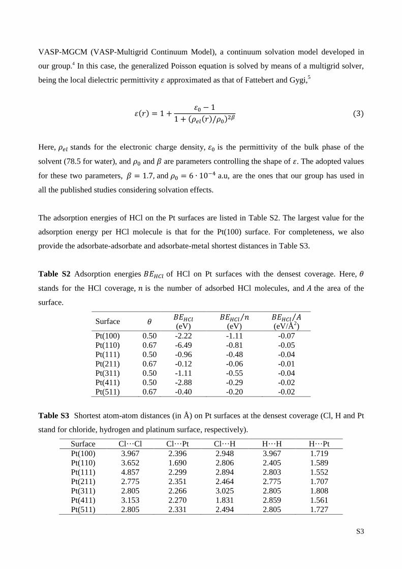
The adsorption energies of HCl on the Pt surfaces are listed in Table S2. The largest value for the

adsorption energy per HCl molecule is that for the Pt(100) surface. For completeness, we also

provide the adsorbate-adsorbate and adsorbate-metal shortest distances in Table S3.

Table S2 Adsorption energies 𝐵𝐸𝐻𝐶𝑙 of HCl on Pt surfaces with the densest coverage. Here, 𝜃

stands for the HCl coverage, 𝑛 is the number of adsorbed HCl molecules, and 𝐴 the area of the

surface.

Surface 𝜃𝐵𝐸𝐻𝐶𝑙

(eV) 𝐵𝐸𝐻𝐶𝑙 𝑛⁄

(eV)𝐵𝐸𝐻𝐶𝑙 𝐴⁄ (eV/Å

2)

Pt(100) 0.50 -2.22 -1.11 -0.07

Pt(110) 0.67 -6.49 -0.81 -0.05

Pt(111) 0.50 -0.96 -0.48 -0.04

Pt(211) 0.67 -0.12 -0.06 -0.01

Pt(311) 0.50 -1.11 -0.55 -0.04

Pt(411) 0.50 -2.88 -0.29 -0.02

Pt(511) 0.67 -0.40 -0.20 -0.02

Table S3 Shortest atom-atom distances (in Å) on Pt surfaces at the densest coverage (Cl, H and Pt

stand for chloride, hydrogen and platinum surface, respectively).

Surface Cl···Cl Cl···Pt Cl···H H···H H···Pt

Pt(100) 3.967 2.396 2.948 3.967 1.719

Pt(110) 3.652 1.690 2.806 2.405 1.589

Pt(111) 4.857 2.299 2.894 2.803 1.552

Pt(211) 2.775 2.351 2.464 2.775 1.707

Pt(311) 2.805 2.266 3.025 2.805 1.808

Pt(411) 3.153 2.270 1.831 2.859 1.561

Pt(511) 2.805 2.331 2.494 2.805 1.727

S4

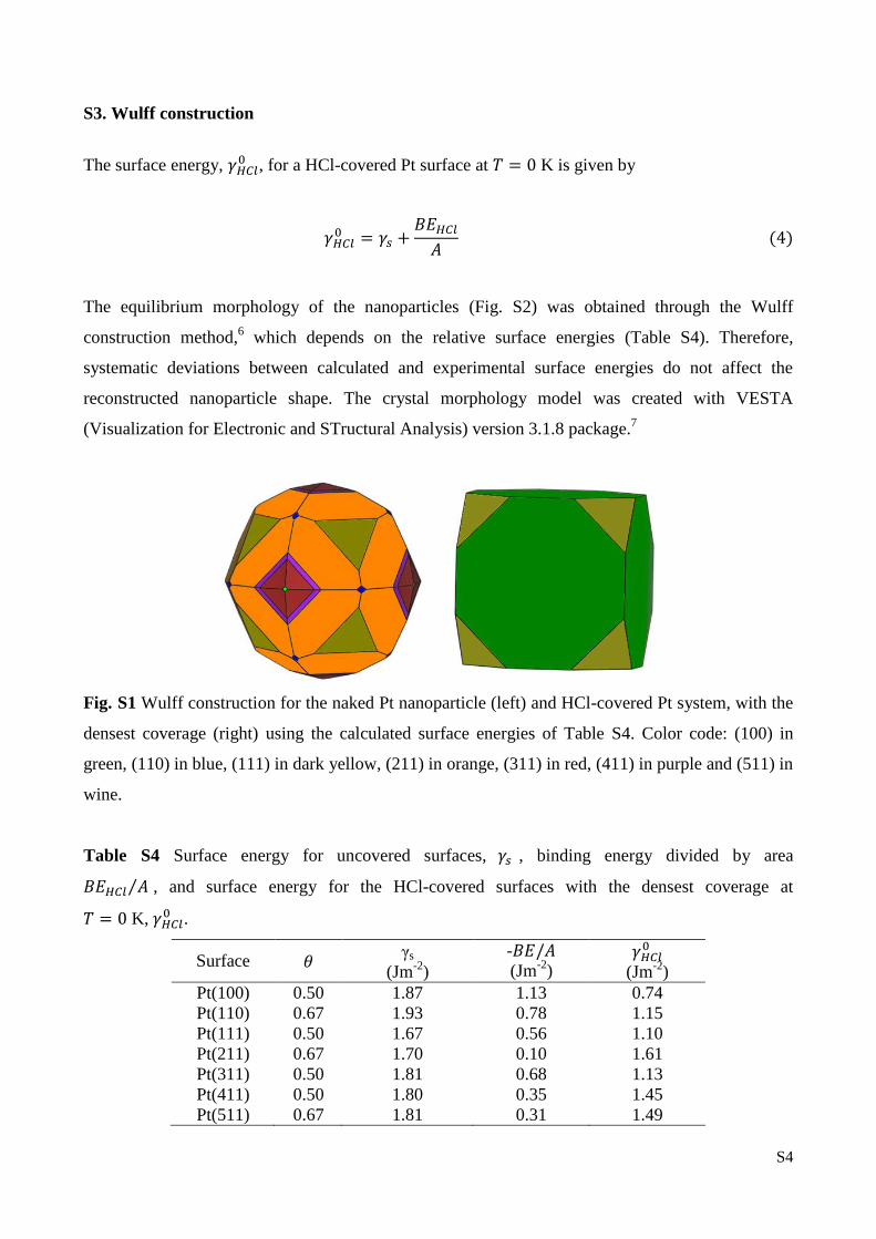
S3. Wulff construction

The surface energy, 𝛾𝐻𝐶𝑙0 , for a HCl-covered Pt surface at 𝑇 = 0 K is given by

𝛾𝐻𝐶𝑙0 = 𝛾𝑠 +

𝐵𝐸𝐻𝐶𝑙

𝐴 (4)

The equilibrium morphology of the nanoparticles (Fig. S2) was obtained through the Wulff

construction method,6 which depends on the relative surface energies (Table S4). Therefore,

systematic deviations between calculated and experimental surface energies do not affect the

reconstructed nanoparticle shape. The crystal morphology model was created with VESTA

(Visualization for Electronic and STructural Analysis) version 3.1.8 package.7

Fig. S1 Wulff construction for the naked Pt nanoparticle (left) and HCl-covered Pt system, with the

densest coverage (right) using the calculated surface energies of Table S4. Color code: (100) in

green, (110) in blue, (111) in dark yellow, (211) in orange, (311) in red, (411) in purple and (511) in

wine.

Table S4 Surface energy for uncovered surfaces, 𝛾𝑠 , binding energy divided by area

𝐵𝐸𝐻𝐶𝑙 𝐴⁄ , and surface energy for the HCl-covered surfaces with the densest coverage at

𝑇 = 0 K, 𝛾𝐻𝐶𝑙0 .

Surface 𝜃γs

(Jm-2

)

-𝐵𝐸/𝐴

(Jm-2

)

𝛾𝐻𝐶𝑙0

(Jm-2

)

Pt(100) 0.50 1.87 1.13 0.74

Pt(110) 0.67 1.93 0.78 1.15

Pt(111) 0.50 1.67 0.56 1.10

Pt(211) 0.67 1.70 0.10 1.61

Pt(311) 0.50 1.81 0.68 1.13

Pt(411) 0.50 1.80 0.35 1.45

Pt(511) 0.67 1.81 0.31 1.49

S5

S4. Ab initio atomistic thermodynamics

S4.1. Theory behind ab initio atomistic thermodynamics

Although DFT methods give a good estimate for a large set of physical quantities, its use is strictly

only valid at 𝑇 = 0 K and 𝑝 = 0 atm. A combination of DFT calculations and thermodynamics

gives a better result for the value of these properties at different thermodynamic conditions. This

approach can be used to compute the different surface energies for a particular arrangement and

coverage of adsorbates, at different conditions of temperature and pressure, or concentration (in the

case we were dealing with solutions).

In order to understand the effect of concentration of different adsorbed species on the stability and

growth of Pt nanoparticle surfaces we employed ab initio atomistic thermodynamics.8 For this

methodology, at constant temperature and pressure, the key magnitude is the Gibbs free energy,

𝐺(𝑇, 𝑝).

If we consider the specific adsorption of HCl on Pt nanoparticles surfaces, the surface energy, 𝛾𝐻𝐶𝑙,

is given by

𝛾𝐻𝐶𝑙 = 𝛾𝑠 + ∆ 𝛾 = 𝛾𝑠 +∆𝐺

𝐴 (5)

where ∆𝐺 stands for the change of the Gibbs free energy. This term can be written as

∆𝐺(𝑇, 𝑝) = 𝐺𝑃𝑡−𝐻𝐶𝑙 (𝑇, 𝑝) − 𝐺𝑃𝑡 (𝑇, 𝑝) − 𝐺𝐻𝐶𝑙 (𝑇, 𝑝) (6)

Here, 𝐺𝑃𝑡−𝐻𝐶𝑙 (𝑇, 𝑝) , 𝐺𝑃𝑡 (𝑇, 𝑝) and 𝐺𝐻𝐶𝑙 (𝑇, 𝑝) are the Gibbs free energies of HCl-covered Pt

surfaces, clean Pt surfaces and HCl molecules, respectively. We present the formulation in terms of

the pressure as done, normally, in the field of heterogeneous catalysis. The first contribution,

𝐺𝑃𝑡−𝐻𝐶𝑙 reads as

𝐺𝑃𝑡−𝐻𝐶𝑙 (𝑇, 𝑝) = 𝐸𝑃𝑡−𝐻𝐶𝑙 𝐷𝐹𝑇 + 𝑝𝑉 − 𝑇𝑆 + 𝑍𝑃𝑉𝐸𝑃𝑡−𝐻𝐶𝑙 (7)

where 𝐸𝑃𝑡−𝐻𝐶𝑙 𝐷𝐹𝑇 is the energy obtained from DFT calculations for the HCl-covered Pt system, 𝑉 is

the system volume, 𝑆 the entropy of the system, and 𝑍𝑃𝑉𝐸𝑃𝑡−𝐻𝐶𝑙 is the calculated zero-point

vibrational energy. The 𝑝𝑉 contribution can be neglected for the bulk since its value is very small as

S6

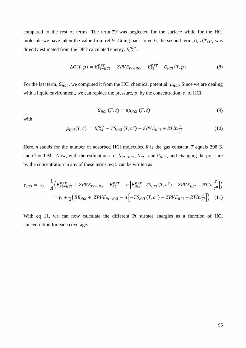
compared to the rest of terms. The term 𝑇𝑆 was neglected for the surface while for the HCl

molecule we have taken the value from ref 9. Going back to eq 6, the second term, 𝐺𝑃𝑡 (𝑇, 𝑝) was

directly estimated from the DFT calculated energy, 𝐸𝑃𝑡𝐷𝐹𝑇.

∆𝐺(𝑇, 𝑝) = 𝐸𝑃𝑡−𝐻𝐶𝑙 𝐷𝐹𝑇 + 𝑍𝑃𝑉𝐸𝑃𝑡−𝐻𝐶𝑙 − 𝐸𝑃𝑡

𝐷𝐹𝑇 − 𝐺𝐻𝐶𝑙 (𝑇, 𝑝) (8)

For the last term, 𝐺𝐻𝐶𝑙 , we computed it from the HCl chemical potential, 𝜇𝐻𝐶𝑙. Since we are dealing

with a liquid environment, we can replace the pressure, 𝑝, by the concentration, 𝑐, of HCl.

𝐺𝐻𝐶𝑙 (𝑇, 𝑐) = 𝑛𝜇𝐻𝐶𝑙 (𝑇, 𝑐) (9)

with

𝜇𝐻𝐶𝑙(𝑇, 𝑐) = 𝐸𝐻𝐶𝑙 𝐷𝐹𝑇 − 𝑇𝑆𝐻𝐶𝑙 (𝑇, 𝑐0) + 𝑍𝑃𝑉𝐸𝐻𝐶𝑙 + 𝑅𝑇𝑙𝑛

𝑐

𝑐0 (10)

Here, 𝑛 stands for the number of adsorbed HCl molecules, 𝑅 is the gas constant, 𝑇 equals 298 K

and 𝑐0 = 1 M. Now, with the estimations for 𝐺𝑃𝑡−𝐻𝐶𝑙 , 𝐺𝑃𝑡 , and 𝐺𝐻𝐶𝑙 , and changing the pressure

by the concentration in any of these terms, eq 5 can be written as

𝛾𝐻𝐶𝑙 = 𝛾𝑠 +1

𝐴(𝐸𝑃𝑡−𝐻𝐶𝑙

𝐷𝐹𝑇 + 𝑍𝑃𝑉𝐸𝑃𝑡−𝐻𝐶𝑙 − 𝐸𝑃𝑡 𝐷𝐹𝑇 − 𝑛 [𝐸𝐻𝐶𝑙

𝐷𝐹𝑇−𝑇𝑆𝐻𝐶𝑙 (𝑇, 𝑐0) + 𝑍𝑃𝑉𝐸𝐻𝐶𝑙 + 𝑅𝑇𝑙𝑛𝑐

𝑐0])

= 𝛾𝑠 +1

𝐴(𝐵𝐸𝐻𝐶𝑙 + 𝑍𝑃𝑉𝐸𝑃𝑡−𝐻𝐶𝑙 − 𝑛 [−𝑇𝑆𝐻𝐶𝑙 (𝑇, 𝑐0) + 𝑍𝑃𝑉𝐸𝐻𝐶𝑙 + 𝑅𝑇𝑙𝑛

𝑐

𝑐0]) (11)

With eq 11, we can now calculate the different Pt surface energies as a function of HCl

concentration for each coverage.

S7

S4.2. Linear fitting data

The surface energies, 𝛾𝐻𝐶𝑙, obtained from the linear fitting are summarized in Table S5 at room

temperature for a range of experimentally relevant HCl concentrations.

Table S5 Surface energies for the HCl-covered surfaces ( 𝛾𝐻𝐶𝑙) , as a function of the HCl

concentration, expressed as percentage (%) and molarity (M). For clarity, we also provide the

values for ln(𝑐 𝑐0⁄ ) in the range used in Fig. 2 in the main text.

𝑐𝐻𝐶𝑙 γHCl(Jm-2

)

% M ln(𝑐 𝑐0⁄ ) 100 110 111 211 311 411 511

0.5 0.16 -1.82 0.77 1.07 1.20 1.19 1.11 1.36 1.08

1 0.32 -1.13 0.75 1.06 1.18 1.18 1.09 1.35 1.06

10 3.24 1.18 0.69 1.02 1.11 1.13 1.02 1.29 0.99

15 4.86 1.58 0.68 1.01 1.10 1.12 1.00 1.28 0.98

25 8.11 2.09 0.67 1.00 1.08 1.11 0.99 1.27 0.96

37 12.10 2.48 0.66 0.99 1.07 1.10 0.97 1.26 0.95

43 13.95 2.64 0.66 0.99 1.07 1.10 0.97 1.25 0.95

50 16.22 2.79 0.65 0.99 1.06 1.09 0.96 1.25 0.94

60 19.46 2.97 0.65 0.99 1.06 1.09 0.96 1.24 0.94

70 22.70 3.12 0.64 0.98 1.05 1.09 0.95 1.24 0.93

80 25.95 3.26 0.64 0.98 1.05 1.08 0.95 1.24 0.93

90 29.19 3.37 0.64 0.98 1.05 1.08 0.95 1.23 0.92

100 32.43 3.48 0.63 0.98 1.04 1.08 0.94 1.23 0.92

The nanoparticle morphology derived from the Wulff construction shown in the inset of Fig. 2 in

the main text was obtained using the surface energies at an experimental HCl percentage in the

water phase of the 25%10

(these data are shown in bold in Table S5).

S8

S5. Pitting values

Fig. S2 DFT-calculated configuration of the Pt365 nanoparticle covered by 119 HCl molecules. The

positions where the pitting can take place are highlighted with a shaded square area (facet), solid

lines (edge), and shaded circles (corner).

Table S6 Reaction energies for the adsorption (+1Pt) and elimination (-1Pt) of a Pt atom at

different positions: facet, edge and corner with respect to the isolated Pt atom.

Structure +1Pt Facet

(eV)

-1Pt Facet

(eV)

-1Pt Edge

(eV)

-1Pt Corner

(eV)

Pt365 -4.43 5.37 4.64 3.62

Pt365(HCl)119 -4.63 4.17 4.16 5.11

S9

S6. Geometrical model for the formation of concave structures

S6.1. Nanoparticle exposed surface and volume

A complementary method to DFT calculations to explain how concave structures are formed from a

nanocube is the use of a geometrical approach. This methodology involves the intersection of the

cube with a solid such that its surface planes correspond to the concave facets of the octapod-like

structures observed experimentally. The point where the intersection starts is crucial to obtain the

desired concave structures. Although not shown here, we have analyzed in detail how the final

structures would look like if the pitting occurred at three different points in the cube: the (i) corners,

(ii) face centers, (iii) edge centers. In this case, the only way to obtain octapods with sharp vertices

involves the pitting occurring at the face centers and towards the center of the cube. In this section,

we describe the process that results in the formation of octapod-like structures using plane geometry

equations.

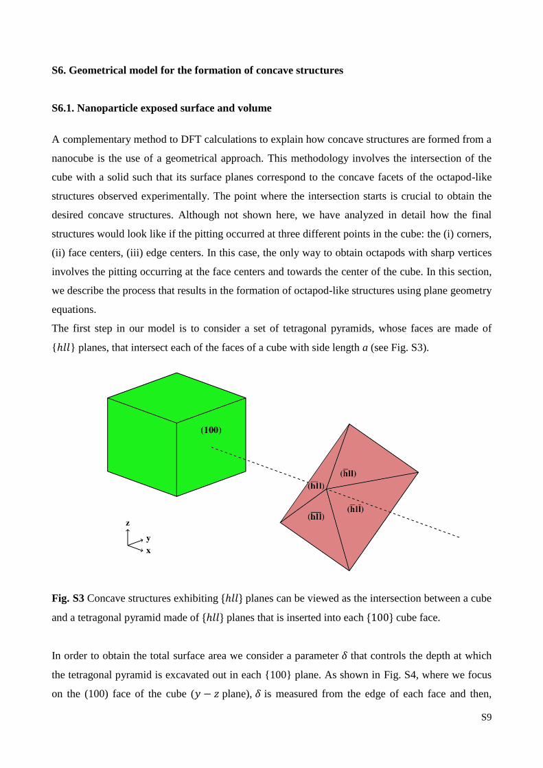
The first step in our model is to consider a set of tetragonal pyramids, whose faces are made of

{ℎ𝑙𝑙} planes, that intersect each of the faces of a cube with side length a (see Fig. S3).

Fig. S3 Concave structures exhibiting {ℎ𝑙𝑙} planes can be viewed as the intersection between a cube

and a tetragonal pyramid made of {ℎ𝑙𝑙} planes that is inserted into each {100} cube face.

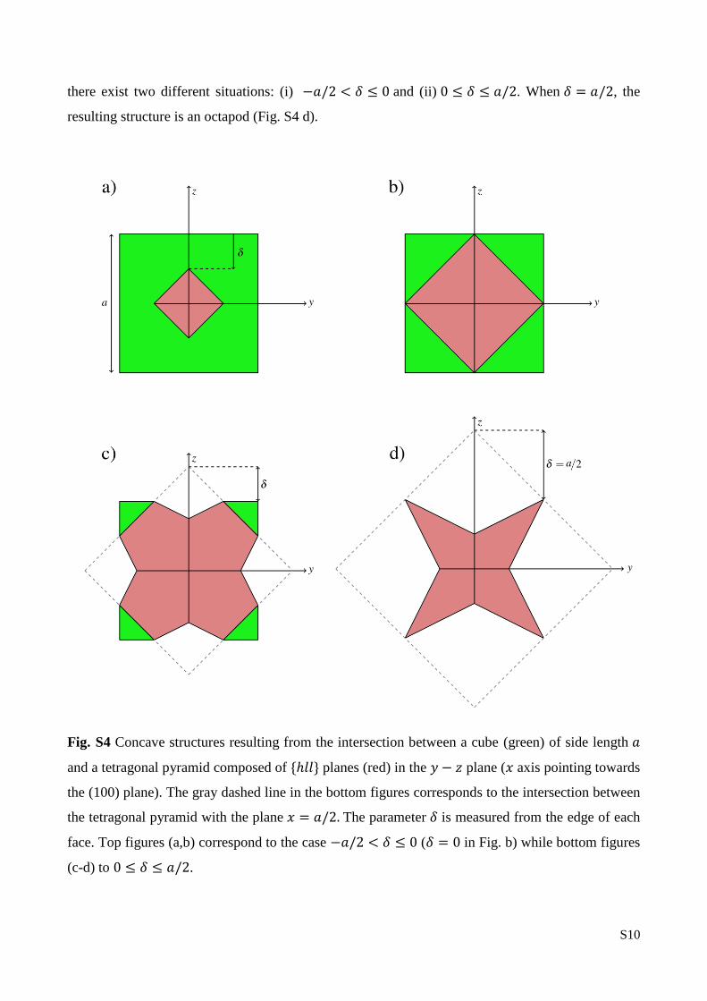
In order to obtain the total surface area we consider a parameter 𝛿 that controls the depth at which

the tetragonal pyramid is excavated out in each {100} plane. As shown in Fig. S4, where we focus

on the (100) face of the cube (𝑦 − 𝑧 plane), 𝛿 is measured from the edge of each face and then,

S10

there exist two different situations: (i) −𝑎/2 < 𝛿 ≤ 0 and (ii) 0 ≤ 𝛿 ≤ 𝑎/2. When 𝛿 = 𝑎/2, the

resulting structure is an octapod (Fig. S4 d).

Fig. S4 Concave structures resulting from the intersection between a cube (green) of side length 𝑎

and a tetragonal pyramid composed of {ℎ𝑙𝑙} planes (red) in the 𝑦 − 𝑧 plane (𝑥 axis pointing towards

the (100) plane). The gray dashed line in the bottom figures corresponds to the intersection between

the tetragonal pyramid with the plane 𝑥 = 𝑎/2. The parameter 𝛿 is measured from the edge of each

face. Top figures (a,b) correspond to the case −𝑎/2 < 𝛿 ≤ 0 (𝛿 = 0 in Fig. b) while bottom figures

(c-d) to 0 ≤ 𝛿 ≤ 𝑎/2.

S11

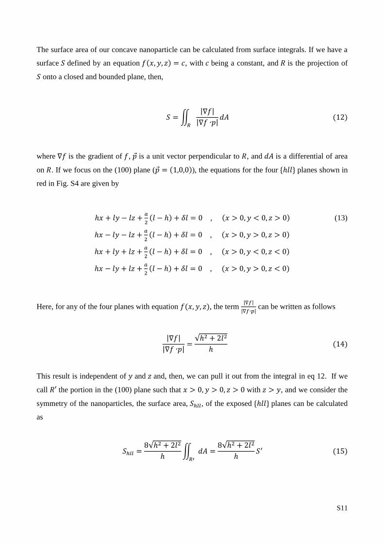
The surface area of our concave nanoparticle can be calculated from surface integrals. If we have a

surface 𝑆 defined by an equation 𝑓(𝑥, 𝑦, 𝑧) = 𝑐, with 𝑐 being a constant, and 𝑅 is the projection of

𝑆 onto a closed and bounded plane, then,

𝑆 = ∬|∇𝑓|

|∇𝑓 ∙𝑝|𝑑𝐴

𝑅

(12)

where ∇𝑓 is the gradient of 𝑓, �⃗� is a unit vector perpendicular to 𝑅, and 𝑑𝐴 is a differential of area

on 𝑅. If we focus on the (100) plane (𝑝 = (1,0,0)), the equations for the four {ℎ𝑙𝑙} planes shown in

red in Fig. S4 are given by

ℎ𝑥 + 𝑙𝑦 − 𝑙𝑧 +𝑎

2(𝑙 − ℎ) + 𝛿𝑙 = 0 , (𝑥 > 0, 𝑦 < 0, 𝑧 > 0) (13)

ℎ𝑥 − 𝑙𝑦 − 𝑙𝑧 +𝑎

2(𝑙 − ℎ) + 𝛿𝑙 = 0 , (𝑥 > 0, 𝑦 > 0, 𝑧 > 0)

ℎ𝑥 + 𝑙𝑦 + 𝑙𝑧 +𝑎

2(𝑙 − ℎ) + 𝛿𝑙 = 0 , (𝑥 > 0, 𝑦 < 0, 𝑧 < 0)

ℎ𝑥 − 𝑙𝑦 + 𝑙𝑧 +𝑎

2(𝑙 − ℎ) + 𝛿𝑙 = 0 , (𝑥 > 0, 𝑦 > 0, 𝑧 < 0)

Here, for any of the four planes with equation 𝑓(𝑥, 𝑦, 𝑧), the term |∇𝑓|

|∇𝑓∙𝑝| can be written as follows

|∇𝑓|

|∇𝑓 ∙𝑝|=

√ℎ2 + 2𝑙2

ℎ (14)

This result is independent of 𝑦 and 𝑧 and, then, we can pull it out from the integral in eq 12. If we

call 𝑅′ the portion in the (100) plane such that 𝑥 > 0, 𝑦 > 0, 𝑧 > 0 with 𝑧 > 𝑦, and we consider the

symmetry of the nanoparticles, the surface area, 𝑆ℎ𝑙𝑙, of the exposed {ℎ𝑙𝑙} planes can be calculated

as

𝑆ℎ𝑙𝑙 =8√ℎ2 + 2𝑙2

ℎ∬ 𝑑𝐴 =

8√ℎ2 + 2𝑙2

ℎ𝑆′ (15)

𝑅′

S12

where 𝑆′ = ∬ 𝑑𝐴𝑅′

. The surface area of the (100) face, 𝑆100, if any, is simply

𝑆100 = 𝑎2 − 8𝑆′ (16)

Then, the total surface area, 𝑆𝑡𝑜𝑡, of each side of the nanoparticle is

𝑆𝑡𝑜𝑡 = 𝑆ℎ𝑙𝑙 + 𝑆100 (17)

In the following, we calculate 𝑆ℎ𝑙𝑙 for 𝛿 < 0 and 𝛿 > 0.

Case 1: −𝒂/𝟐 ≤ 𝜹 ≤ 𝟎

In this case, 𝑅′ is defined as

𝑅′ = {𝑦 ≤ 𝑧 ≤

𝑎

2+ 𝛿 − 𝑦

0 ≤ 𝑦 ≤1

2(

𝑎

2+ 𝛿)

} (18)

For clarity we also show this region in Fig. S5 a.

Fig. S5 Integration region 𝑅′ for 𝛿 < 0 (a) and 𝛿 > 0 (b).

S13

The surface area of 𝑅′, called 𝑆′, is calculated straightforwardly

𝑆′ = ∫ ∫ 𝑑𝑧𝑑𝑦 = ∫ (𝑎

2+ 𝛿 − 2𝑦) 𝑑𝑦 =

1

4(

𝑎

2+ 𝛿)

212

(𝑎2

+𝛿)

0

𝑎2

+𝛿−𝑦

𝑦

12

(𝑎2

+𝛿)

0

(19)

Then, using eq 15 we calculate 𝑆ℎ𝑙𝑙 as

𝑆ℎ𝑙𝑙 =2√ℎ2 + 2𝑙2

ℎ(

𝑎

2+ 𝛿)

2

(20)

Here, 𝑆100 is computed using eq 16.

Case 2: 𝟎 ≤ 𝜹 ≤ 𝒂/𝟐

The region 𝑅′ is now defined as (see also Fig. S5 b)

𝑅′ = {𝑦 ≤ 𝑧 ≤

𝑎

2+ 𝛿 − 𝑦

0 ≤ 𝑦 ≤1

2(

𝑎

2+ 𝛿)

} − {

𝑎

2≤ 𝑧 ≤

𝑎

2+ 𝛿 − 𝑦

0 ≤ 𝑦 ≤ 𝛿}

− {

𝑙𝑦

(ℎ − 𝑙)+

𝑎(ℎ − 𝑙) − 2𝛿𝑙

2(ℎ − 𝑙)≤ 𝑧 ≤

𝑎

20 ≤ 𝑦 ≤ 𝛿

} (21)

The second and third term correspond to the blue and white triangles shown in Fig. S5 b,

respectively. The surface area 𝑆′ can be calculated as for the previous case (𝛿 < 0), but now we

need to subtract the area of both triangles. The base and height of the blue triangle are equal to 𝛿,

whereas for the white triangle they equal 𝛿 and 𝑑 = 𝛿𝑙/(ℎ − 𝑙), respectively. Then,

𝑆′ =1

4(

𝑎

2+ 𝛿)

2

−𝛿2

2−

𝛿2𝑙

2(ℎ − 𝑙)=

1

4(

𝑎

2+ 𝛿)

2

−𝛿2ℎ

2(ℎ − 𝑙) (22)

S14

For 𝑆100, in the case 𝛿 > 0, we can not use 𝑆′ as defined in eq 22 as, here, we should not consider

the area of the white triangle. Then,

𝑆100 = 𝑎2 − [2 (𝑎

2+ 𝛿)

2

− 4𝛿2] (23)

As done before, we just need to consider the symmetric shape of the nanoparticle using eq 15 to

compute 𝑆ℎ𝑙𝑙,

𝑆ℎ𝑙𝑙 =√ℎ2 + 2𝑙2

ℎ[2 (

𝑎

2+ 𝛿)

2

−4𝛿2ℎ

(ℎ − 𝑙)] (24)

Due to the fact that both eqs 20 and 24 are equal except for the last term in eq 24, we can introduce

a Heaviside step function, 𝜃(𝛿) and write 𝑆ℎ𝑙𝑙(𝛿) as follows

𝑆ℎ𝑙𝑙(𝛿) =√ℎ2 + 2𝑙2

ℎ[2 (

𝑎

2+ 𝛿)

2

−4𝛿2ℎ

(ℎ − 𝑙)𝜃(𝛿)] (25)

where 𝜃(𝛿) is given by

𝜃(𝛿) = {1, 𝛿 > 00, 𝛿 ≤ 0

(26)

Fig. S6 shows 𝑆𝑡𝑜𝑡 as a function of 𝑆100 for ℎ = 3, 𝑙 = 1 and 𝑎 = 1.0 (in arb. units).

S15

Fig. S6 Total surface area, 𝑆𝑡𝑜𝑡, of each side of the nanoparticle as a function of the area of the

(100) face, 𝑆100, for the case ℎ = 3, 𝑙 = 1, and 𝑎 = 1 (arb. units).

In order to compute the surface-area-to-volume ratio we have calculated the volume, 𝑉, of the

nanoparticle as a function of 𝛿. In this case, 𝑉 also has a different functional form depending on the

sign of 𝛿. We do not provide here the whole set of equations used to compute 𝑉 but just give its

final functional form.

𝑉𝛿≤0 = 𝑎3 −𝑙

2ℎ(𝑎 + 2𝛿)3 (27)

𝑉𝛿≥0 = 𝑎3 − [𝑙

2ℎ(

𝑎(ℎ − 𝑙) − 2𝛿𝑙

ℎ − 𝑙)

3

+3𝛿𝑙

(ℎ − 𝑙)3(𝑎(ℎ − 𝑙) − 2𝛿𝑙)2 +

8𝑙2𝛿3

(ℎ − 𝑙)2+

12𝛿2𝑙ℎ

(ℎ − 𝑙)2(

𝑎

2− 𝛿)

+8𝛿3𝑙ℎ(ℎ − 2𝑙)

(ℎ − 𝑙)3] (28)

When 𝛿 = 0 both eqs 27 and 28 yield the same value 𝑉𝛿=0 = 𝑎3(1 − 𝑙/2ℎ).

S16

Another result to point out is that we cannot have octapods for any combination of the Miller

indices such that ℎ > 𝑙 and 𝑙 = 𝑘. This result can be easily obtained if we look at eq 13 for any of

the planes and we set 𝛿 = 𝑎/2. In this case, there should exist some thickness, 𝑥0, in the 𝑥-axis at

the point where the four planes intersect each other (at 𝑦 = 0 and 𝑧 = 0, see Fig. S4 d). Looking at

any of the four planes, and setting 𝛿 = 𝑎/2, we have the following result

𝑥0 =(ℎ − 2𝑙)

ℎ

𝑎

2 (29)

which means that we can only have octapod-like concave nanoparticles when ℎ > 2𝑙. Then, (311),

(411) and (511) facets can be present in octapods, but not {211} or {433} planes, a result that

agrees with experimental observations where mainly (311) and (411) faces have been reported.

S6.2. Relationship of 𝜹 with the HCl concentration

The parameter 𝛿 is a function of the concentration 𝑐 of HCl. The concentration at which the

nanoparticles adopt the different shapes can be determined experimentally from TEM

measurements and then one can assess the functional form of 𝛿(𝑐). In the case of 𝛿 depending

linearly on 𝑐:

𝛿 = −𝑎

2+

𝑎

𝑐2 − 𝑐1

(𝑐 − 𝑐1) (30)

where 𝑐1 stands for the concentration at which nanocubes are formed, while 𝑐2 corresponds to the

value at which octapods are observed. At 𝑐 = (𝑐2 + 𝑐1)/2 the situation is that shown in Fig. S4 b

(𝛿 = 0). For eq 30 to be true, the side length of the nanoparticle should be equal to 𝑎 during the

etching process. The parameter 𝛿 can also depend on 𝑐 as a power law 𝛿(𝑐) ∝ (𝑐 − 𝑐1)𝛼 with

𝛼 > 1 or 𝛿(𝑐) ∝ (𝑐/𝑐1)−𝛽 with 𝛽 > 1. Then, once the dependence 𝛿(𝑐) is determined, one just

need to enter a value for 𝑐 in eq 30 in the range [𝑐1, 𝑐2] to calculate 𝛿 and then the total nanoparticle

exposed surface and volume would be obtained through eqs 17, 23, 25, 27 and 28.

S17

References

(1) N. E. Singh-Miller and N. Marzari, Phys. Rev. B, 2009, 80, 235407.

(2) R. Tran, Z. Xu, B. Radhakrishnan, D. Winston, W. Sun, K. A. Persson and S. P. Ong, Sci. Data,

2016, 3, 160080.

(3) W. R. Tyson and W. A. Miller, Surf. Sci., 1977, 62, 267-276.

(4) M. Garcia-Ratés and N. López, J. Chem. Theo. Comp., 2016, 12, 1331-1341.

(5) J.-L. Fattebert and F. Gygi, J. Comput. Chem., 2002, 23, 662-666.

(6) G. Wulff, Z. Krystallogr. Mineral, 1901, 34, 449-530.

(7) K. Momma and F. Izumi, J. Appl. Crystallogr., 2011, 44, 1272-1276.

(8) K. Reuter and M. Scheffler, Phys. Rev. B, 2002, 65, 035406.

(9) D. D. Ebbing, S. D. Gammon, General Chemistry, 9th ed.; Houghton Mifflin Company, Boston,

MA, 2009.

(10) R. A. Martı́nez-Rodrı́guez, F. J. Vidal-Iglesias, J. Solla-Gullón, C. R. Cabrera and J. M. Feliu,

J. Am. Chem. Soc., 2014, 136, 1280-1283.