shape optimization of wind turbine blades using panel methods

Shape optimization of windturbine blades using panelmethods

Master of Science thesis

A.S. Bravo

Shape optimization ofwind turbine bladesusing panel methods

Master of Science thesisby

A.S. Bravoto obtain the degree of:

Master of Science in Aerospace Engineering at Delft University of TechnologyMaster of Science in Engineering (Eurpoean Wind Energy) at Technical University of

Denmarkto be defended publicly on Monday August 16, 2021 at 9:00h.

Student number TU Delft: 5130581Student number DTU: s193081Project duration: November 1, 2020 – July 31, 2021Supervisors: Professor Ole Sigmund, DTU

Associate professor Sergio Turteltaub, TU DelftPostdoctoral researcher Cian Conlan-Smith, DTUAssociate professor Casper Schousboe Andreasen, DTU

An electronic version of this thesis is available at http://repository.tudelft.nl/.

http://repository.tudelft.nl/

Abstract

Wind turbines play an increasingly imporant role in the energy production of our time.In order to optimize the performance of wind turbine blades, this thesis work aims at as-sessing the possibility of using panel methods for gradient based optimization of the aero-dynamics of wind turbine blades. Specifically, the method employed has used Dirichletboundary condition, a fixed wake for optimization and a free wake model for validation.The panel method developed has been validated against the MIRAS software and CFD re-sults. The results of the optimization are compared against the Glauert optimum blade.The blade is parameterized using NACA profiles and the twist and chord are used as de-sign variables. Two optimizations have been performed: an unconstrained optimization,which has shown to take advantage of limitations of the panel method model; a secondoptimization is performed applying a thrust constraint and with tighter bounds on the de-signs variables, which is capable of achieving realistic results. The main conclusion is thatrealistic blade designs can be achieved using a fixed wake panel method for aerodynamicoptimization, although ultimately the performance of these designs should be assessed us-ing higher fidelity models.

iii

Preface

This thesis marks the end of my two year education programme as student of the EuropeanWind Energy Master in the Rotor Design track - Structures. I have learned a lot during thisperiod of time, but above all it has been a period of huge personal development. For this Ineed to thank all the fellow students of the EWEM programme, who have shared this uniqueexperience with me, and also everyone involved in the organization of the programme;creating a master among four universities is no easy task, but you sure are doing a good jobat it.

The Msc thesis itself has been the culmination of this 2 year programme, and as wellas the programme itself it has been a joint effort of the universities of DTU and TU Delft.I’d like to thank the thesis supervisors from both universities: Sergio Turteltaub from TUDelft and Ole Sigmund, Casper Schousboe Andreasen and Cian Conlan-Smith from DTUfor sharing their time and experience with me. The regular meetings held throughout thepast 9 months have been invaluable to keep the thesis going on the right path.

Finally, I would like to thank everyone who has encouraged me in any way in the courseof this thesis work. To this regard, I would like to thank my parents for their inconditionalsupport. Also, I appreciate incredibly the daily morning coffees with Thomas, offline andonline, which have kept going during the whole duration of the thesis. It was the motor ofmy days, thank you for that.

A.S. BravoKongens Lyngby, July 2021

v

List of Figures

3.1 Domain and boundaries of interest for the potential flow formulation . . . . . 93.2 Streamlines of a point source. . . . . . . . . . . . . . . . . . . . . . . . . . . . . . 93.3 Streamlines of a doublet pointing in the x direction. . . . . . . . . . . . . . . . 93.4 Pressure coefficient of a NACA 4412 at an angle of 4 degrees. Results of the

2D implementation of a panel method compared against experimental data.Experimental data extracted from M. Pinkerton [1937] . . . . . . . . . . . . . . 13

3.5 Representation of a the wind turbine blade model. Blade number 1 is meshed,while blades 2 and 3 are accounted for via symmetry. The x axis points to-wards the document, following the right hand rule. . . . . . . . . . . . . . . . . 14

3.6 Representation of a conical fixed wake model. . . . . . . . . . . . . . . . . . . . 153.7 Convergence study on the wake model using an Euler forward model f = 0,

an Euler backward ( f = 1) and a predictor-corrector scheme ( f = 0.5). . . . . . 173.8 a) NREL 5MW airfoils and b) Zoom on the TE . . . . . . . . . . . . . . . . . . . 193.9 a) Modified NREL 5MW airfoils and b) Zoom on the TE . . . . . . . . . . . . . . 193.10 Comparison of normal a) and tangential b) forces on the NREL 5MW rotor

blades using CFD , MIRAS and the currently developed code. Extracted fromRamos-García et al. [2014]. The first point from assto has been excluded forvisualization purposes. . . . . . . . . . . . . . . . . . . . . . . . . . . . . . . . . . 20

3.11 Normal force to the rotor along the span . . . . . . . . . . . . . . . . . . . . . . 213.12 Tangential force to the rotor along the span . . . . . . . . . . . . . . . . . . . . 213.13 Normal force to the rotor along the span . . . . . . . . . . . . . . . . . . . . . . 213.14 Tangential force to the rotor along the span . . . . . . . . . . . . . . . . . . . . 213.15 Normal force to the rotor along the span . . . . . . . . . . . . . . . . . . . . . . 213.16 Pressure distribution at the tip . . . . . . . . . . . . . . . . . . . . . . . . . . . . 21

4.1 Decomposition of velocities at a spanwise section of the wing. [To be substi-tuted by own figure, extracted from Hansen [2015]] . . . . . . . . . . . . . . . . 24

4.2 Relation between angle of attack, inflow angle and twist. . . . . . . . . . . . . . 254.3 Optimal axial and tangential inductions as calculated with Glauert’s theory. . 254.4 Ideal chord as calculated using Glauert’s theory, with and without root and tip

corrections applied. . . . . . . . . . . . . . . . . . . . . . . . . . . . . . . . . . . 264.5 Ideal twist distribution as calculated using Glauert’s theory. . . . . . . . . . . . 264.6 Axial induction in the glauert blade as computed with panel methods and

BEM theory. . . . . . . . . . . . . . . . . . . . . . . . . . . . . . . . . . . . . . . . 274.7 Moment around the x axis for the glauert blade as computed with panel meth-

ods and BEM theory. . . . . . . . . . . . . . . . . . . . . . . . . . . . . . . . . . . 27

5.1 Representation of the parameterization of an airfoil using the NACA 4 digitseries. . . . . . . . . . . . . . . . . . . . . . . . . . . . . . . . . . . . . . . . . . . . 30

vii

viii List of Figures

5.2 Sensitivities of Mx with respect to the chord for different fixed wake modelsand the free wake model computed for the Glauert optimal blade. . . . . . . . 32

5.3 Sensitivities of Mx with respect to the twist for different fixed wake modelsand the free wake model computed for the Glauert optimal blade. . . . . . . . 32

5.4 Problem 1: Spanwise chord distribution for different s f values. . . . . . . . . . 345.5 Problem 1: Spanwise twist distribution for different s f values. . . . . . . . . . 345.6 Problem 1: Spanwise moment distribution on the optimized blades. Loads

computed using a free wake model. . . . . . . . . . . . . . . . . . . . . . . . . . 345.7 Problem 2: Spanwise axial induction on the optimized blades. Velocities

computed using a free wake model. . . . . . . . . . . . . . . . . . . . . . . . . . 345.8 Problem 2: spanwise chord distribution for different thrust constraints; s f =

0.5. . . . . . . . . . . . . . . . . . . . . . . . . . . . . . . . . . . . . . . . . . . . . 355.9 Problem 2: spanwise twist distribution for different thrust constraints; s f = 0.5. 355.10 Problem 2: spanwise chord distribution for different thrust constraints; s f =

0.75. . . . . . . . . . . . . . . . . . . . . . . . . . . . . . . . . . . . . . . . . . . . . 365.11 Problem 2: spanwise twist distribution for different thrust constraints; s f =

0.75. . . . . . . . . . . . . . . . . . . . . . . . . . . . . . . . . . . . . . . . . . . . . 365.12 Problem 2: spanwise chord distribution for different thrust constraints; s f =

1.0. . . . . . . . . . . . . . . . . . . . . . . . . . . . . . . . . . . . . . . . . . . . . 365.13 Problem 2: spanwise twist distribution for different thrust constraints; s f = 1.0. 365.14 Problem 2: Local angle of attack of the blade obtained with T<42 and s f = 0.5. 375.15 Problem 2: spanwise axial induction distribution for different thrust con-

straints; s f = 0.5. . . . . . . . . . . . . . . . . . . . . . . . . . . . . . . . . . . . . 385.16 Problem 2: spanwise Mx distribution for different thrust constraints; s f = 0.5. 385.17 Problem 2: spanwise axial inductiond distribution for different thrust con-

straints; s f = 0.75. . . . . . . . . . . . . . . . . . . . . . . . . . . . . . . . . . . . . 385.18 Problem 2: spanwise Mx distribution for different thrust constraints; s f = 0.75. 385.19 Problem 2: spanwise axial induction distribution for different thrust con-

straints; s f = 1.0. . . . . . . . . . . . . . . . . . . . . . . . . . . . . . . . . . . . . 385.20 Problem 2: spanwise Mx distribution for different thrust constraints; s f = 1.0. 38

A.1 Normal force to the rotor along the span for different chord discretizations. . 43A.2 Tangential force to the rotor along the span for different chord discretizations. 43A.3 Normal force to the rotor along the span for different spanwise discretizations. 44A.4 Tangential force to the rotor along the span for different spanwise discretiza-

tions. . . . . . . . . . . . . . . . . . . . . . . . . . . . . . . . . . . . . . . . . . . . 44A.5 Normal force to the rotor along the span for different number of wake revolu-

tions. . . . . . . . . . . . . . . . . . . . . . . . . . . . . . . . . . . . . . . . . . . . 44A.6 Tangential force to the rotor along the span for different number of wake rev-

olutions. . . . . . . . . . . . . . . . . . . . . . . . . . . . . . . . . . . . . . . . . . 44A.7 Normal force to the rotor along the span for different number of wake panels

per revolution. . . . . . . . . . . . . . . . . . . . . . . . . . . . . . . . . . . . . . 44A.8 Normal force to the rotor along the span for different number of wake panels

per revolution. . . . . . . . . . . . . . . . . . . . . . . . . . . . . . . . . . . . . . . 44

B.1 Relative error between the finite difference sensitivities and the adjoint sen-sitivities for the objective function. . . . . . . . . . . . . . . . . . . . . . . . . . . 46

List of Figures ix

B.2 Relative error between the finite difference sensitivities and the adjoint sen-sitivities for the constraint functions. . . . . . . . . . . . . . . . . . . . . . . . . 46

C.1 Flowchart of the code. . . . . . . . . . . . . . . . . . . . . . . . . . . . . . . . . . 48

List of Tables

5.1 Operating conditions of the wind turbines set for the optimization problems. 295.2 Mesh discretization parameters employed for optimization. . . . . . . . . . . . 305.3 Problem 1: performance of the three optimized blades in terms of power and

coefficient of power. . . . . . . . . . . . . . . . . . . . . . . . . . . . . . . . . . . 355.4 Problem 2: performance of the optimized blades in terms of power and coef-

ficient of power. . . . . . . . . . . . . . . . . . . . . . . . . . . . . . . . . . . . . . 37

A.1 Baseline discretization used for comparison with other coarser and finer meshes. 43

xi

Nomenclature

Acronyms

AEP Annual Energy Production

BEM Blade Element Momentum

CFD Computational Fluid Dynamics

COE Cost of Energy

CoP Coefficient of Power

DNS Direct Numerical Simulation

FD Finite Difference

LES Large Eddy Simulation

MDO Multidisciplinary Design Optimization

MMA Method of Moving Asymptotes

RANS Reynolds Averaged Navier-Stokes

TP Trefftz Plane

TSR Tip Speed Ratio

VLM Vortex Lattice Method

WT Wind Turbine

Symbols

Ω Angular speed of the rotor

n Vector normal to panel

q Velocity vector

r Position in body centered coordinate system

v∞ Inflow velocity at the rotor

vp Perturbed velocity

vref reference velocity

xiii

xiv Nomenclature

µ Doublet strength

Φ Potential of the velocity

ρ Air Density

σ Dynamic viscosity/Source strength

Ai Doublet influence coefficient of blade and wake

Bi Source Influence coefficient

c Reference length (chord)

Ci Doublet influence coefficient of blade/wake

CP Pressure coefficient

f Body force

g acceleration of gravity

Re Reynolds number

SB Body surface

Sr ot Rotor area

SW Wake surface

s f shortening factor; related to wake length

u speed in the x direction.

v Speed in the y direction.

w Speed in the z direction.

a axial induction factor

a’ Tangential induction factor

B number of rotor blades

p Pressure

Contents

List of Figures vii

List of Tables xi

Nomenclature xiii

1 Introduction 1

2 Literature Study 32.1 Choice of objective . . . . . . . . . . . . . . . . . . . . . . . . . . . . . . . . . . . . 32.2 Exploration of the design space . . . . . . . . . . . . . . . . . . . . . . . . . . . . . 32.3 Aerodynamic models . . . . . . . . . . . . . . . . . . . . . . . . . . . . . . . . . . . 4

3 Aerodynamic modelling 73.1 Potential flow theory . . . . . . . . . . . . . . . . . . . . . . . . . . . . . . . . . . . 7

3.1.1 Source and doublet strength . . . . . . . . . . . . . . . . . . . . . . . . . . 103.1.2 System of linear equations . . . . . . . . . . . . . . . . . . . . . . . . . . . 113.1.3 Load calculation. . . . . . . . . . . . . . . . . . . . . . . . . . . . . . . . . . 123.1.4 2D example . . . . . . . . . . . . . . . . . . . . . . . . . . . . . . . . . . . . 123.1.5 Modelling of symmetry . . . . . . . . . . . . . . . . . . . . . . . . . . . . . 13

3.2 Wake modelling . . . . . . . . . . . . . . . . . . . . . . . . . . . . . . . . . . . . . . 133.2.1 General considerations . . . . . . . . . . . . . . . . . . . . . . . . . . . . . 143.2.2 Fixed wake . . . . . . . . . . . . . . . . . . . . . . . . . . . . . . . . . . . . . 153.2.3 Free wake . . . . . . . . . . . . . . . . . . . . . . . . . . . . . . . . . . . . . . 15

3.3 Validation of the aerodynamic model . . . . . . . . . . . . . . . . . . . . . . . . . 173.3.1 Validation case study . . . . . . . . . . . . . . . . . . . . . . . . . . . . . . . 173.3.2 Spanwise loads on the rotor. . . . . . . . . . . . . . . . . . . . . . . . . . . 183.3.3 Pressure distribution along the span . . . . . . . . . . . . . . . . . . . . . 203.3.4 Discussion on the validation . . . . . . . . . . . . . . . . . . . . . . . . . . 20

4 Glauert’s optimum rotor 234.1 Glauert’s Optimal rotor . . . . . . . . . . . . . . . . . . . . . . . . . . . . . . . . . . 234.2 Analysis of Glauert’s rotor using Panel Methods . . . . . . . . . . . . . . . . . . . 25

5 Aerodynamic Optimization 295.1 Setup of the Optimization . . . . . . . . . . . . . . . . . . . . . . . . . . . . . . . . 29

5.1.1 Operating conditions. . . . . . . . . . . . . . . . . . . . . . . . . . . . . . . 295.1.2 Discretization of the blade . . . . . . . . . . . . . . . . . . . . . . . . . . . 29

5.2 Parameterization . . . . . . . . . . . . . . . . . . . . . . . . . . . . . . . . . . . . . 295.3 Filtering . . . . . . . . . . . . . . . . . . . . . . . . . . . . . . . . . . . . . . . . . . . 305.4 Search strategy and sensitivities . . . . . . . . . . . . . . . . . . . . . . . . . . . . 315.5 Validation of the Optimization . . . . . . . . . . . . . . . . . . . . . . . . . . . . . 325.6 Definition and results of the optimization problems . . . . . . . . . . . . . . . . 33

xv

xvi Contents

6 Conclusions and recommendations 396.1 Conclusions . . . . . . . . . . . . . . . . . . . . . . . . . . . . . . . . . . . . . . . . 396.2 Recommendations for future work . . . . . . . . . . . . . . . . . . . . . . . . . . . 40

A Effect of Discretization on the loads 43

B Finite Difference checks 45

C Code structure and contribution 47

Bibliography 49

1Introduction

It is undeniable that wind turbines play a major role in the energy production of our time;in 2019 the electricity produced by wind turbines alone represented 15% of the total energyconsumed in the European Union [Wind Europe, 2020] and it is foreseen that the share ofwind in the energy market will continue to increase [IEA, 2020, GWEC, 2020]. There is muchfocus in the optimization of wind turbines to make them more efficient and be able to drivethe cost of energy down in order to make this form of energy more competitive in the mar-ket. Specifically, blades represent a very important share of the cost of manufacturing awind turbine, and the energy production itself highly depends on them. MultidisciplinaryDesign Optimization (MDO) is a growing approach because it is necessary to achieve trade-offs between the aerodynamics and structure of the blade to achieve an optimum design.Considering only aerodynamic motivations, the airfoils would be chosen to be thin to beable to maximize power extraction. However, this is not possible because the structure re-quires thicker airfoils, specially close to the root, to be able to fulfill the requirements of tipdisplacement and bending moments, among others [Bottasso et al., 2016]. In this sense, itis important to perform mulditidciplinary optimization of wind turbine blades, as opposedto sequential monodisciplinary optimizations, in order to improve the design of wind tur-bine blades.

The aerodynamic design variables in MDO can range from chord and twist distributionof the profiles [Bottasso et al., 2016] to full shape optimization of a WT blade, including theshape of the airfoils in the design, as in Kenway et al. [2010], Bottasso et al. [2014], Mad-sen et al. [2019]. For the structural part, one choice is to use the size and position of somepre-assumed elements such as spars, cap spars, trailing edge reinforcement, etc. and opti-mize those. One example, out of many in the literature, is Sessarego and Shen [2018] whichpreassumes a box-spar shape of the inner structure. The problem of this approach is that itmakes use of the structural elements that are already known and being used at the moment,thus limiting considerably the design space. An attempt for a more general approach in thestructural design was made by Wang et al. [2020]: the blade was discretized by a 1D beamin the longitudinal direction while at different spanwise sections of the blade 2D topologyoptimization was performed. In the aerospace field, James et al. [2014] goes further andperforms topology optimization on a full wing using 3D brick elements. However, both ap-proaches face the same obstacle: the meshes employed to discretize the structure of theblade and wing, respectively, do not have enough resolution to see any actual substruc-tures like spars or ribs arise. The 2D topology approach from Wang et al. [2020] has the

1

2 1. Introduction

further drawback that neighbouring sections are connected only through a beam model,thus making the appearance of 3D substructures difficult.

After reviewing the work done by other authors in the past in the literature, to the knowl-edge of the author, multidisciplinary optimization has not been performed on wind turbineblades using a gradient based approach. The aim of this thesis work is to start to coverthis gap. Specifically, this project will build on the previous work carried in DTU by CianConlan-Smith as part of his doctoral thesis. In the article Conlan-Smith et al. [2020] theaerodynamic shape of an aircraft wing was optimized using a panel method as aerody-namic model. On later work [Conlan-Smith and Schousboe Andreasen, 2020] MDO op-timization of an aircraft wing performing simultaneous aerodynamic and structural opti-mization adding a Timoshenko beam model to the panel method to calculate the structuraldisplacements and loads.

The objective of this thesis work is to optimize the aerodynamic shape of a wind turbineblade using a panel method and a gradient based search algorithm, and test whether panelmethods are an appropriate tool to be used for MDO in wind turbine blade design.

The report is structured as follows: chapter 2 makes a review of the existing literatureon multidisciplinary optimization and specifically on aerodynamic modelling of wind tur-bines; chapter 3 presents the aerodynamic model employed and a validation of it; chapter4 presents Glauert’s optimal rotor, which will be used later on as benchmark of comparisonfor the optimization results; chapter 5 presents the results of the aerodynamic optimiza-tion and compares them against the Glauert rotor presented previously; finally, chapter 6concludes the thesis project and gives advice on how to proceed with the established work.

2Literature Study

In the introduction chapter the most relevant work similar to this project was describedbriefly. An important part of the challenge of WT optimization lays in making an appro-priate choice of methods for the optimization. In the following sections the most commonchoices in the literature are outlined, which will later help motivate the choice of methodsfor this thesis project. Specifically, the topics touched upon are: the choice of an appro-priate objective function for optimization, the search strategy of the design space and theaerodynamic model used to compute aerodynamic loads.

2.1. Choice of objectiveWhen performing simultaneous aerodynamic and structural optimization one has to makea choice of objectives for the optimization. One option is to perform multi-objective op-timization, improving at the same time aerodynamic and structural variables. This is theapproach chosen in Fischer et al. [2014], where Thrust, Mass and Annual Energy Produc-tion (AEP) are optimized simultaneously. A different direction is to try to convert the severalcompeting objectives into a single one, for example using a weighted sum of the objectivesas the problem objective. Wang et al. [2020] applies this approach using different weightsfor the power coefficient Cp and the structural compliance. A popular approach, essen-tially equivalent to the weighted sum, is to use the Cost of Energy (COE) as figure of merit,employed for example in Bottasso et al. [2016] and Ashuri et al. [2014]. This approach triesto take into account in one single function the combination of the cost of manufacturing,transport, maintenance, etc. of the wind turbine and the expected energy output. The Costof Energy is the real driving factor in industry when designing a wind turbine. However,determining the cost function of a wind turbine can be tricky when performed in an auto-matic optimization approach since some of the costs are difficult to obtain [Bottasso et al.,2016].

2.2. Exploration of the design space

There are several strategies in which the design space can be explored. A popular optionis to use gradient-free approaches such as Evolutionary Algorithms [Fischer et al., 2014,Vianna Neto et al., 2018]. Evolutionary Algorithms are very good at exploiting non-smooth

3

4 2. Literature Study

design spaces, are in general easy to implement and are very well suited for multi-objectiveoptimization. However, they tend to be slow and show poor convergence. Gradient-basedapproaches [Bottasso et al., 2016, Wang et al., 2020] are comparatively more complex toimplement and explore a narrower region of the design space, but are computationallymuch more efficient and need fewer iterations to converge, which is why they are deemedmore appropriate for high-fidelity implementations. On the other side, gradient-based ap-proaches have a tendency to get stuck around local optima and are sensitive to the initialconditions. Still another approach is surrogate modelling, as used by Sessarego and Shen[2018]. By feeding several blade designs to the algorithm, for which each of them the massis optimized in an inner loop, a simplified explicit function of the Cost of Energy on the de-sign variables is found. In this case the design variables being the chord, twist and relativethickness of the blade. The maximum of the COE simplified function is then found by agrid search approach, which ensures that the global optimum will be found.

2.3. Aerodynamic modelsThe objective of this subsection is to give an overview of the aerodynamic models that areemployed for load calculation on wind turbine blades. In the future this information willhelp motivate the choice of an aerodynamic method for the aerostructural optimization ofa wind turbine blade.

The aerodynamic models that are more used for load calculation on wind turbines arelisted below:

• Blade Element Momentum (BEM)

• Vortex Methods

• Euler

• Reynolds Averaged Navier-Stokes (RANS)

• Large Eddy Simulation (LES)

• Direct Numerical Simulation (DNS)

The methods are organized from lower fidelity to higher fidelity, and from low to highcomputational cost, starting from BEM up until DNS. A brief overview of these methods,including its main strengths and weaknesses, will be presented in the following alineas.The reader is referred to Hansen et al. [2006] for a more thorough overview on the topic.

The momentum theory was first developed by Rankine and Froude, and extended byGlauert to account for 2D effects. The rotor is modelled by an actuator disc, divided intoconcentric annular streamtubes. The streamtubes are assumed to be independent fromeach other and the number of blades is assumed to be infinite. The theory makes use of thefundamental principles of mass conservation, axial and angular momentum balances andenergy conservation to every control volume (streamtube); added to the blade element the-ory, the local flow conditions can be calculated assuming that the 2D profiles of the bladeact independently of surrounding elements. The combined approach, which we call BEMtheory, allows the calculation of the aerodynamic forces and the induced velocities at the

2.3. Aerodynamic models 5

rotor. The BEM theory is limited to axial induction factors of 0.5; however, this can be ex-tended for a higher range of induction factors with the introduction of empirical formulas[Wang, 2012]. Similarly, several corrections have been introduced over the years to accountfor effects of stall delay, dynamic stall, stall misalignment, etc. [Thé and Yu, 2017].

BEM is the most used design tool seen in the literature for optimization purposes [Mad-sen et al., 2019]. It combines mass and momentum balance equations on the rotor with 2Dairfoil data at specific spanwise positions of the blade to obtain loads in every spanwiseposition. The reason why it is so popular is because of its easy implementation and lowcomputational cost. However, it also has many deficiencies. The flow is assumed to staywithin so called stream tubes, so it can’t model 3D rotational effects. Other phenomenalike yaw misalignment, dynamic stall, etc. are only accounted for using semiempirical cor-rections. Additionally, it must be noted that due to some of its assumptions the effects ofnon-planar blade geometries (e.g. blade pre-bend or tip winglets) cannot be accountedfor [Lawton and Crawford, 2014]. For more information on the BEM theory the reader canrefer to Hansen [2015].

Vortex methods model the aerodynamics of a blade (or wing) based on vortices. Theinfluence of these vortices is calculated using the Biot-savart law. Vortex methods can ingeneral refer to several models: Lifting Line, Vortex Lattice Method (VLM) , and Panel Meth-ods, which can be used to model the lifting surfaces of a blade and the wake, or only thewake. The wake can be modelled in three different ways: Rigid (or fixed) wake, prescribedwake and free wake models. A rigid wake doesn’t take into account the expansion of thewake, a prescribed wake makes use of numerical and experimental analysis to decide on awake position and free wake models locate the wake based on the effects of all aerodynamiccomponents involved in the model, but doing so results in an increased computational cost[Wang, 2012].

Of the vortex methods mentioned, the focus of this thesis will be put on Panel Methods[Hess, 1973] because of its ability to model 3D surfaces accurately, which is an indispens-able requisite of the research formulation in order to be able to optimize the external shapeof a wind turbine. The other two methods are limited to small angles of attack and thinairfoils [Peerlings, 2018]. The method is simple to implement and doesn’t require a mesh.It gives better insight into the dynamics of the flow than the BEM method, since every el-ement of the blade considered affects every other point of the domain. It is for examplepossible to calculate cases of yaw misalignment and dynamic inflow [Blondel et al., 2016].Since vortex methods assume inviscid flow, viscosity and stall are not included in the modeland the only source of drag is induced drag. For the same reason rotational augmentationcannot be accounted for, as they arise mainly from perturbations on the viscous boundarylayer along the spanwise and chordwise direction due to centrifugal and coriolis forces, re-spectively. Rotational effects increase the lift coefficient at high angles of attack and causestall delay, so it is beneficial for the perfomance of the blade [Wang, 2012]. Two aerostruc-tural analyses that have made use in the past of panel methods are Conlan-Smith and Sc-housboe Andreasen [2020] and James et al. [2014] applied to the optimization of aircraftwings, and Sessarego et al. [2016] for the optimization of wind turbine blades.

RANS is the highest fidelity Computational Fluid Dynamics (CFD) method that still canbe used with relative frequency in the wind turbine industry for optimization purposes[Madsen et al., 2019]. As RANS works with time-integrated quantities, it cannot cover all

6 2. Literature Study

time-dependent phenomena, such as unsteady flow separation and vortex shedding [Théand Yu, 2017]. Still, it is able to account for viscosity, 3D effects, rotational augmentationand turbulence with an appropriate choice of a turbulence model. However, it is compu-tationally more expensive than BEM and vortex methods, and requires meshing of the 3Ddomain.

Higher fidelity models are LES, which calculates the effect of large eddies and modelsthe sub gridscale eddies, and DNS, which resolves directly all scales of turbulence. How-ever, they are considered computationally too expensive to be applied to a wind turbineflow field [Wang, 2012], hence they won’t be considered further in this review.

3Aerodynamic modelling

This chapter of the thesis describes the aerodynamic model later employed to carry outthe blade optimization. The model is based on the previous work by Cian Conlan-Smith;see references Conlan-Smith et al. [2020], and Conlan-Smith and Schousboe Andreasen[2020], in which aerodynamic and aero-structural optimization of wings was carried outusing a panel method code. This thesis aims to build on that work to add capabilities forthe load calculation and optimization of rotating blades. Appendix C explains specificallythe structure of the software and the additions made in this project.

Section 3.1 explains the basics of potential flow theory and the most important deriva-tions regarding panel methods. Section 3.2 explains the wake model that was implementedfor the rotating blade, which is the major change made with respect to the static wing case.Lastly, section 3.3 discusses and compares the results against other aerodynamic models tovalidate the results of the present code.

3.1. Potential flow theoryThis section presents the fundamentals of potential flow theory. Only a brief summary ofthe theoretical derivations is presented here, in order to put the work of this thesis in con-text. The derivations are based on the book by Katz and Plotkin [2004]; for further detailson the topic the reader is referred to this book.

To characterize the velocity field and loads around a body we will require two sets ofequations. The first one is the continuity equation for an incompressible fluid:

∇·q = ∂u

∂x+ ∂v

∂y+ ∂w

∂z= 0 (3.1)

The second set of equations are the Navier-Stokes equations, which characterize themotion of a newtonian fluid. They represent the momentum balance on the fluid, thusrelating the acceleration with the stresses on the fluid; on the most general form they canbe written:

ρ

(∂qi

∂t+q ·∇qi

)= ρ fi − ∂

∂xi

(p + 2

3µ∇·q

)+ ∂

∂x jµ

(∂qi

∂x j+ ∂q j

∂xi

)(i = 1,2,3) (3.2)

Where ρ is the fluid density, is the dynamic viscosity coefficient, p is the pressure. q isthe velocity vector, f is a body force.

7

8 3. Aerodynamic modelling

However, the Navier-Stokes in its general form do not have an explicit solution; an ex-plicit solution can only be found for very few simplified cases. If we assume inviscid flowwe obtain the so-called Euler equation:

∂q

∂t+q ·∇q = f− ∇p

ρ(3.3)

It can be demonstrated via dimensional analysis (see Katz and Plotkin [2004]) that theouter flow around a body can be assumed inviscid for high values of the Reynolds number.The Reynolds number is presented in eq. 3.4, where u here is a reference windspeed and c areference length, which could be the chord of a blade for the case being. In a high Reynoldsflow the inertial forces are in magnitude more relevant than the viscous forces, hence theviscosity can be neglected in the outer region of the flow. However, close to the surface ofthe blade the shear stresses gain importance and the viscosity can no longer be neglectedwithout affecting the accuracy of the solution.

Re = ρuc

µ(3.4)

A further premise that will be necessary in order to obtain the potential flow equationis the assumption that the flow is irrotational. The definition of rotational flow is tied to theconcept of vorticity. For a highly viscous flow, the shear forces are relevant and will causeflow particles to rotate; oppositely, if the shear forces are irrelevant the flow particles willnot rotate and the flow can be regarded as irrotational. It can be demonstrated, again, thatfor high reynolds numbers the generation of vorticity outside of the boundary layer can beneglected, thus it is possible to make the assumption of irrotational flow.

With the condition that the flow is irrotational, the velocity can be written as the dif-ferential of a scalar function of the position. This function be called the potential Φ of thevelocity:

q =∇Φ (3.5)

Then, from eq. (3.1) and (3.5), the Laplace equation is obtained:

∇·q =∇·∇Φ=∇2Φ= 0 (3.6)

Solving the Laplace equation gives information about the velocity field around a body.However, in order to calculate the aerodynamic forces around an airfoil, it is necessary toconnect the velocity field with the pressure field. For this, the Euler equation (3.3) needsto be used. For an irrotational, incompressible flow, taking gravity as the only conservativeforce acting on the fluid and in static conditions, the Euler equation can be reduced to theBernoulli equation:

g z + p

ρ+ q2

2+ ∂Φ

∂t= const . (3.7)

The equation tells us that at any given point in space, the left hand side is equal to aconstant. Therefore, the left hand side will be equal for a pair of points in space at anychosen moment in time. This will allow later to compute the pressure distribution arounda body once the flow around it is resolved.

3.1. Potential flow theory 9

Figure 3.1: Domain and boundaries of interest for the potential flow formulation

Consider the general domain depicted in figure 3.1. Without entering in the theoret-ical details, the potential at any point of the domain can be written as the integral of thecontribution of sources and doublets distributed in the boundaries:

Φ(P ) =− 1

4π

∫SB

[σ

(1

r

)−µn ·∇

(1

r

)]dS + 1

4π

∫SW

[µn ·∇

(1

r

)]dS +Φ∞(P ) (3.8)

In turn, doublets (µ) and sources (σ) are defined as:

−µ=Φ−Φi (3.9)

−σ= ∂Φ

∂n− ∂Φi

∂n(3.10)

Note that the variable µ, which has been used previously in the flow equations, is nowused to designate the doublet strength. From now on µ will only be used for this purpose.

Figure 3.2: Streamlines of a point source. Figure 3.3: Streamlines of a doublet pointing in the xdirection.


Doublets and sources are elementary solutions that satisfy the Laplace equation. Thevelocity field generated by point sources and doublets has been depicted in figures 3.2 and3.3. It is important to note that the solution to the Laplace equation can be obtained byplacing doublets and sources on the boundaries of the problem. In general, though, thereis not unique distribution of solutions that will satisfy the Laplace equation, hence a choicebased on physical considerations needs to be made.

The problem described above is solved by defining boundary conditions at the surfaces.There are two ways to do this: by enforcing so-called Neumann or Dirichlet boundary con-ditions. A Neumann boundary condition specifies the value of the derivative of the poten-tial at the surface. This has a directly relatable physical meaning, and it is equivalent tospecifying that the velocity normal to the surfaces needs to be zero. Dirichlet boundaryconditions, instead, define the value of the potential itself at the boundary. This results in alower computational cost for the type of problem this thesis works on Conlan-Smith et al.[2020], hence the focus will be put on this second type of boundary conditions.

It can be demonstrated that the inner potential of a closed surface follows the expres-sion:

Φ∗i (x, y, z) = 1

4π

∫SB+SW

µ∂

∂n

(1

r

)dS − 1

4π

∫SB

σ

(1

r

)dS +Φ∞ = const. (3.11)

Now, the inner potential can be chosen conveniently (Φ∗i = Φ∞) so that equation (3.11)

reduces to:1

4π

∫SB+SW

µ∂

∂n

(1

r

)dS − 1

4π

∫SB

σ

(1

r

)dS = 0 (3.12)

Equation (3.12) will be used to reduce the problem to a linear system of equations thatcan be solved easily by means of well established linear algebra tools, as will be explainednext.

3.1.1. Source and doublet strengthNow that the theoretical bases for potential flow have been set, it is necessary to knowthe numerical procedure to find a solution for a discretized aerodynamic body. For thepanel method we are dealing with this means determining the strength of the sources anddoublets along the surface.

From the condition that the velocity normal to the surface must be zero (the so-calledNeumann condition), and the definition of a source (3.10), follows that the strength of asource panel needs to be:

σ= n ·vref (3.13)

vref = [v∞−Ω× r] (3.14)

Where n is normal to the body surface, pointing inside, v∞ is the inflow velocity at therotor, Ω is the angular speed of the wind turbine rotor and r is the position of a point inbody coordinates. vref is the flow velocity seen by the body, which is different for everysection of the blade.

At this point the strength of the doublets is not uniquely defined. This arises from thefact that infinite values of circulation, or equivalently lift, are possible for a given sourcedistribution. To determine the strength of the doublets at each panel, it is necessary toenforce some physical consideration so that the amount of circulation, and hence the lift,is the correct one.

3.1. Potential flow theory 11

The condition that we are going to use is called the Kutta condition; it is based on em-pirical observation, and it essentially states that the flow on an airfoil will leave the trailingedge smoothly. Therefore, as the flow approaches the trailing edge, the velocity at the up-per and lower surfaces will need to be equal. Specifically, it is required that the trailing edgeis a stagnation point (of zero velocity) when the trailing edge has a finite angle, but a finitevelocity can exist for cusped trailing edges. Mathematically, for the case of a panel methodusing a doublet distribution to generate lift, the Kutta condition can be written as:

µU −µL −µW = 0 (3.15)

Where the subindices refer to the upper and lower surface of the airfoil and the wake,respectively. Expression 3.15 tells us that there is a jump in circulation at the trailing edge ofthe airfoil, which is equal to the wake circulation. For further insight on the mathematicaldevelopment of this expression, the reader is referred to Katz and Plotkin [2004]. Anderson[2017] also covers comprehensively the Kutta condition and its physical explanation. Theconcept of circulation, which has been mentioned here, can also be consulted in thesesources.

Additionally to eq. 3.15, the doublets are required to have constant strength along thewake, and the wake shape should be parallel to local streamlines. As will be explained later,when talking about the wake model in section 3.2, it is not immediate how to satisfy thissecond condition. If the geometry of the wake is prescribed in advance, this condition willbe, at best, an approximation. Other methods, which don’t require a predetermined wakeshape, involve solving the geometry of the wake iteratively until a converged shape thatfulfills the physical requirements is achieved.

3.1.2. System of linear equationsNow assume that the body is discretized into N panels, and the wake is discretized into NW

panels. It will also be assumed from now on that the strength of the doublet and the sourcesin the panels are constant. We can now rewrite equation 3.12 for a discrete body as:

N∑k=1

Ckµk +NW∑`=1

C`µ`+N∑

k=1Bkσk = 0 (3.16)

Equation 3.16 must be true for every panel’s collocation point. The collocation pointis where the boundary condition is enforced; it is located at the center of the panel andslightly inside the body, since the Dirichlet boundary condition (eq. 3.12) needs to be en-forced at an inner point of the body. Equation 3.16 expresses that for every collocationpoint, the sum of the contributions of potential of all the other panels needs to be zero.The contribution of every influencing panel is its Influence Coefficient (Ck ,Cl ,Bk ), whichdepends on its relative position to the collocation point, times the strength of the influenc-ing panel. The influence coefficients are calculated as:

Ck = 1

4π

∫S

∂

∂n

(1

r

)dS

∣∣∣∣k

(3.17)

Bk = −1

4π

∫S

(1

r

)dS

∣∣∣∣k

(3.18)


The exact evaluation of these integrals depends on the choice of panel of the model. Forconstant strength quadrilateral panels, as used in this work, the expressions are derived inKatz and Plotkin [2004], section 10.4.

As seen previously in equation 3.13, the source strengths (σ) can be determined be-forehand. The wake doublet strengths can be put as a function of the surface strengths(eq. 3.15). Therefore, the problem of solving eq. 3.12 ultimately corresponds to solving thefollowing system of linear equations:

N∑k=1

Akµk =−N∑

k=1Bkσk (3.19)

Where the matrix A is the matrix C with the contributions from the wake panels.

3.1.3. Load calculationThe total velocity vtot at a certain point of the body will be the inflow (or reference) velocity(eq. 3.14) plus the perturbation caused by the panels of the body and the wake (vp):

vtot = vref +vp (3.20)

Now, neglecting the height term and considering that the problem at hand is steady-state (hence ∂Φ

∂t = 0) eq. 3.7 can be used to compute the coefficient of pressure at everypanel of the body:

CP = p −pr e f

1/2ρv2r e f

= 1− v2tot

v2r e f

(3.21)

Note that the reference velocity here used accounts for the rotational speed of the bladeand therefore will have a different value for every spanwise location, each section seeing anincreasingly high velocity moving towards the tip. Finally, the contribution of a panel to theaerodynamic forces on the body will be:

∆F =−CP

(1

2ρv2

ref

)∆Sn (3.22)

Which if integrated over specific spanwise position will give the normal and tangentialforces in that section.

3.1.4. 2D exampleNow let’s look at the results from a 2D panel method code to better understand what thesekinds of methods are capable of and also their limitations. Figure 3.4 shows the CP distri-bution over the chord of a NACA 4412 profile for a Reynolds number of 3 ·106. The panelmethod shows that the CP distribution follows a similar shape than the experimental data,but it clearly overestimates the suction at the upper side of the airfoil. The main reasonbehind these differences is the inviscid assumption of the panel method. Since viscosityhas been neglected for the theoretical model, the figure shows (as expected) that the liftloads will be overestimated. For higher accuracy, the panels have been placed in a cosinedistribution along the chord, so that the mesh is more dense towards the leading edge andthe trailing edge. This increases the acccuracy of the solution for a given number of panels,since these are the regions where the CP suffers more drastic changes.

3.2. Wake modelling 13

Figure 3.4: Pressure coefficient of a NACA 4412 at an angle of 4 degrees. Results of the 2D implementation ofa panel method compared against experimental data. Experimental data extracted from M. Pinkerton [1937]

3.1.5. Modelling of symmetryThe blades of a wind turbine are identical and equally spaced at regular angles. Assumingthat the pitch of the blades is also the same, the rotor has rotational symmetry, which canbe used to reduce the model that will be employed for the analysis. Only one blade needsto be meshed instead of discretizing the whole rotor. Since the strengths of the singularitieswill be the same for every blade, the system of equations can also be reduced and has thesize of one blade mesh.

The way symmetry is exploited is during the calculation of the influence coefficients.Specifically, blade 1 (schematically represented in figure 3.5) is modelled and solved. Forevery collocation point of the blade, the influence of the other panels of blade 1 are com-puted. Then a simple transformation is applied to that panel (eq. 3.23) to find the co-ordinates of the corresponding panels of blades 2 and 3. While the influence coefficientsare still computed for all the panels in the three blades (or any corresponding number ofblades), this procedure allows to solve a system of equations of size equal to the panels inone blade. Since solving the system of equations is a very costly part of the program, thisallows for a huge decrease in computational cost. x

yz

k=2,3

= 1 0 0

0 cosΨk −sinΨk

0 sinΨk cosΨk

xyz

1

(3.23)

3.2. Wake modellingThree different ways to model the wake of a wind turbine will be distinguished, from lowerto higher complexity: fixed wake, prescribed wake and free-wake models. The geometry ofa fixed (or rigid) wake is determined as an input and doesn’t change during the analysis. Itis the simpler model still able to capture the physics of a wind turbine, even though it needsappropriate user input to provide reliable results. A prescribed wake is a simplified model


Figure 3.5: Representation of a the wind turbine blade model. Blade number 1 is meshed, while blades 2 and3 are accounted for via symmetry. The x axis points towards the document, following the right hand rule.

that gives a wake geometry as a function of some simplified parameters. For example, Ro-bison et al. [1995] proposes a model to calculate the wake geometry as a function of theinduction at the blades. This allows the implementation of an iterative scheme where theblade induction is updated until convergence. This type of methods are tested and tunedfor existing wind turbine data, but it might not be the best approach to testing novel WT ge-ometries [Vermeer et al., 2003]. The third method is the free-wake approach. In this modelthe interaction between wake filaments/panels is accounted for. The wake shape is com-puted iteratively until the conditions of equation 3.24 are met. Here below the fixed andfree wake methods that have been implemented will be commented on; however, there areseveral other free wake methods that can be consulted for example in Leishman [2006] andKatz and Plotkin [2004].

3.2.1. General considerationshe governing equations and the resulting system of linear equations used to solve the dou-blet strength for each panel have been discussed previously in section 3.1. It has also beenshown how to compute the wake strength as a function of the trailing edge doublets usingthe Kutta condition. The effect of the wake has been mentioned there. However, until nowthe computation of the wake geometry is a topic that has not been touched upon. Thissubsection will briefly discuss general principles that determine the wake shape.

A doublet panel of the wake should respect the condition that it should not generatelift, because it is not a solid surface (see Katz and Plotkin [2004]), this can be expressed as:

q×∇µW = 0 (3.24)

Hence, the boundaries of the wake panels should be parallel to the local velocity. Sincethe wake geometry is obviously not known beforehand, this will require iterative methodsto find a converged solution. The family of methods that attempts to find a wake that fol-lows equation 3.24 are called free wake methods.

3.2. Wake modelling 15

Figure 3.6: Representation of a conical fixed wake model.

3.2.2. Fixed wakeA fixed wake is a model that represents the vorticity shed by the blades independently fromthe parameters of the model. The geometry is chosen beforehand and is not updated dur-ing the design. Therefore, a degree of experience and previous knowledge on wake geome-tries is required to achieve acceptable results using a fixed wake model.

The implementation of the fixed wake model allows for an improvement of the com-prehension on how the wake geometry will affect the loads on the wind turbine. Figure3.6 shows a representation of the fixed wake employed in the model. The two parametersthat can be changed are a cone angle and a length factor, which determines the velocity atwhich the wake is propagating. Note that it is assumed that the wake panels shed at thesame instant will remain in-line —there is no shear parallel to the x direction—.

The parameter s f , which stands for shortening factor, is defined below with regards tothe fixed wake model, as it will be useful later on.

s f = uw ake

u∞(3.25)

s f measures the ratio of the speed of the wake and the undisturbed speed. To exemplifythis, for s f = 1 the wind turbine would not be slowing the wind down at all, while for s f =0.5 the wind turbine is slowing the wind to half the inflow speed.

3.2.3. Free wakeThe free-wake model implemented is similar to the method proposed in Katz and Plotkin[2004], referred to as time-stepping model for a steady state case. The equation that rulesthe motion of the panels of the wake is the following one:

dr

dt= vref(r)+vp(r) (3.26)

where the term vref refers to the velocity due to the change in the reference system, andvp(r) is the induced (or perturbed) velocity.

Different numerical schemes are possible to solve equation 3.26, namely explicit, hy-brid and implicit. Explicit methods are simple conceptually; however, they are prone tonumerical issues related with round-off errors (see Leishman [2006], p.618).

Two different methods have been implemented in the present code, both described inLeishman [2006]. The first one is an time-stepping Euler explicit approach. The second one


is an approach close to the predictor-corrector scheme described in the former reference,which is a two-step explicit approach.

Let’s start by describing the Euler explicit approach. The first iteration is conductedusing the fixed wake geometry described in sec. 3.2.2. The velocities are calculated at everypoint and then every point is propagated using the velocity information:

rn+1 = rn +∆t ·vp(rn)+∆rr e f (3.27)

Where the term ∆rref(rn) accounts for the fact that the body frame of reference is rotat-ing. The superindices n and n+1, respectively, refer to the current and future time steps. Inthis method the points are trailed based on the velocity calculated at the current position,hence no information of the future step is required and there is no need to solve a systemof equations.

Leishman [2006], p.618 suggests that Euler explicit methods do not present consistentconvergence, but rather can start oscillating after some iterations. This will be discussed forthe present case further down this section. For this reason, a predictor-corrector schemewas implemented for the wake.

The predictor-corrector scheme consists of two explicit stages. In the first stage an ap-proximation of the wake geometry rn+1 is made using eq. 3.28. The geometry at time-stepn+1 is then used to approximate the perturbation velocity (vp(rn+1)). This first stage allowsto know the velocity at the future time-step without actually solving a system of equations,as would be the case for an implicit method. The second stage of the predictor-correctorscheme follows eq. 3.29:

rn+1 = rn +∆t ·vp(rn)+∆rr e f (3.28)

rn+1 = rn +∆t · ((1− f ) ·vp(rn)+ f ·vp(rn+1))+∆rr e f (rn) (3.29)

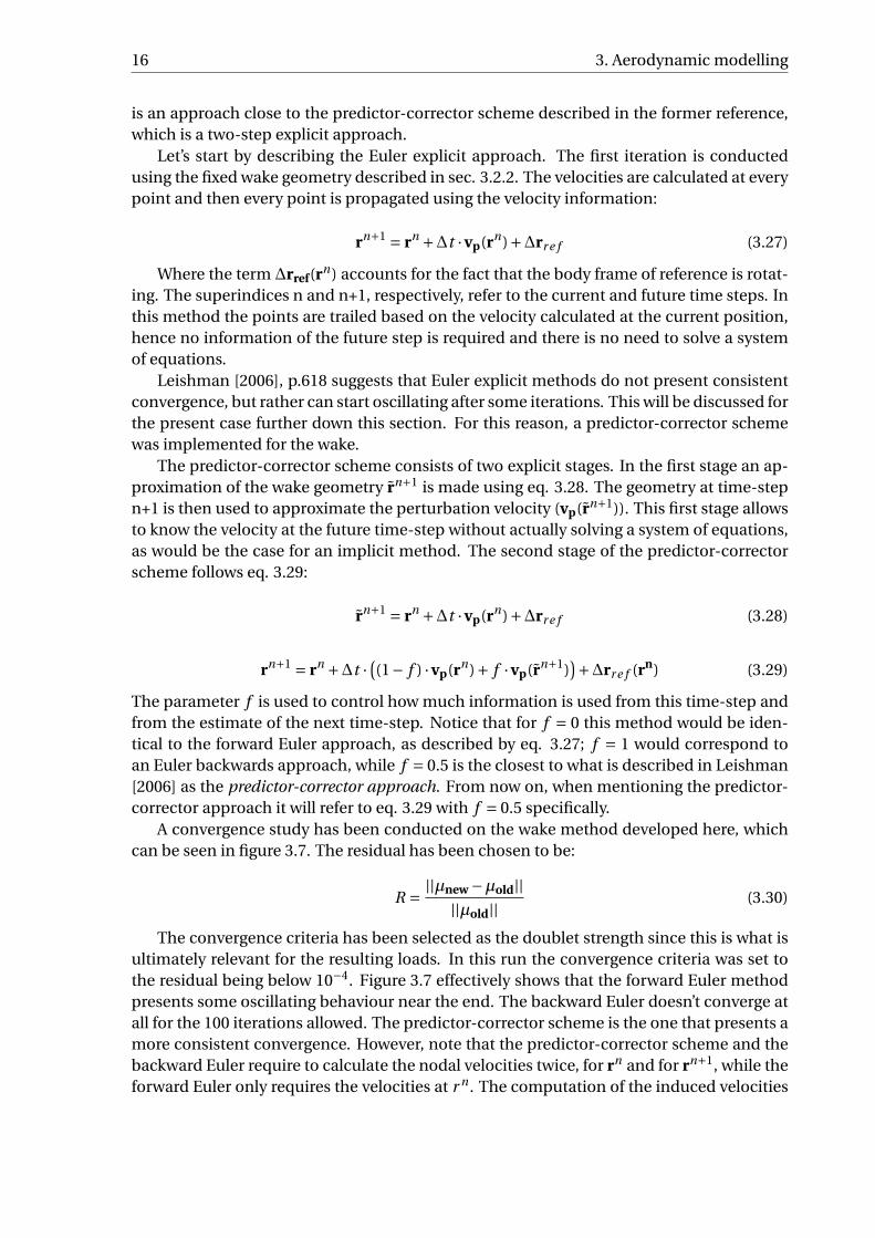
The parameter f is used to control how much information is used from this time-step andfrom the estimate of the next time-step. Notice that for f = 0 this method would be iden-tical to the forward Euler approach, as described by eq. 3.27; f = 1 would correspond toan Euler backwards approach, while f = 0.5 is the closest to what is described in Leishman[2006] as the predictor-corrector approach. From now on, when mentioning the predictor-corrector approach it will refer to eq. 3.29 with f = 0.5 specifically.

A convergence study has been conducted on the wake method developed here, whichcan be seen in figure 3.7. The residual has been chosen to be:

R = ||µnew −µold||||µold||

(3.30)

The convergence criteria has been selected as the doublet strength since this is what isultimately relevant for the resulting loads. In this run the convergence criteria was set tothe residual being below 10−4. Figure 3.7 effectively shows that the forward Euler methodpresents some oscillating behaviour near the end. The backward Euler doesn’t converge atall for the 100 iterations allowed. The predictor-corrector scheme is the one that presents amore consistent convergence. However, note that the predictor-corrector scheme and thebackward Euler require to calculate the nodal velocities twice, for rn and for rn+1, while theforward Euler only requires the velocities at r n . The computation of the induced velocities

3.3. Validation of the aerodynamic model 17

Figure 3.7: Convergence study on the wake model using an Euler forward model f = 0, an Euler backward( f = 1) and a predictor-corrector scheme ( f = 0.5).

is a costly computation, which means that doubling this computation represents a con-siderable increase in the overall running wall-clock time. The Predictor-corrector schemetakes on average ≈ 65% more time per iteration of the wake than the explicit Euler. For mostruns, it is considered that a residual of 10−3 is enough to consider the code converged. Inthat range of accuracy, the Euler forward method seems to be the best trade-off between ac-curacy and computational cost and as such will be the primary choice for the optimizationruns.

3.3. Validation of the aerodynamic modelIn this section the developed panel code will be compared against the results from the MI-RAS software. MIRAS is also a panel method code and has been validated extensively be-fore, which makes it convenient to compare the results of this thesis work against it.

This section will first explain the case that is being used to validate the code, that is theNREL 5MW geometry (see NREL 5MW report by Jonkman et al. [2009]). The next subsec-tion is a comparison of the normal and tangential forces along the blade span, followed bya study on the pressure distribution on some sample sections along the blade. The last sub-section is a discussion of the results obtained, which includes a discussion on them with anexpert on panel methods, the researcher Néstor Ramos-García, who is the main developerof the MIRAS code.

3.3.1. Validation case studyThe results of the simulations of this thesis are compared, specifically, against the article byRamos-García et al. [2014].

While essentially the presently developed panel code and the MIRAS model are bothpanel codes, there are some differences in the implementation that must be noted to thereader, which are mentioned hereunder. MIRAS is a computational panel code that usesthe Neumann no-penetration condition to enforce the boundary conditions. The present


code, on the contrary, uses a Dirichlet BC. The code can be run with and without account-ing for viscosity, which is taken into account by coupling the panel code to a viscous bound-ary layer solver, Q3UIC. The wake is modelled using a free-wake model that employs trailingfilaments to account for the influence of the wake on the flow field. Oppositely, the presentcode uses quadrilateral panels to model the wake.

In the mentioned article, MIRAS is run on several wind turbine rotors. For the presentcomparison, we will take the results from the analyses on the NREL 5MW rotor. The NREL-5MW is a fictitious wind turbine to be used by researchers, aimed at testing new models andmethods of analysis, as well as new technologies, to be able to compare easily the resultsof those studies on a common-ground wind turbine. The reference turbine is an upwind,variable-speed, pitch controlled machine. The aerodynamic, structural and control param-eters necessary for an analysis are provided in the NREL report. The aerodynamic sectionsare provided at different stages of the blade, along with their corresponding polars (Cl −αand Cd −α plots). Together with the chord and twist values at each section, this is enoughto conduct an analysis with a BEM code. However, for CFD or a panel code the exact geom-etry is needed, which is not provided in the original NREL 5MW report. This is why severalresearchers who have used this baseline turbine need to take some freedom into decidinghow to model the geometry.

For several sections along the blade, the parameters given in the NREL report are radius,chord, twist and the specific airfoil used in the section. A further assumption needed isregarding the center of the blade axis. It is assumed that the blade axis is straight and that itis located at 25% of the chord for every airfoil section. The twist is therefore applied at eachblade center.

The second additional modification has to do with the airfoil shape. The original airfoils(see figure 3.8) which can be found in the original NREL report have blunt trailing edges,which is a problem when running panel method simulations. In these cases, enforcingthe Kutta condition is problematic. The kutta condition helps determine the amount ofcirculation around an airfoil, given that the flow leaves the trailing edge smoothly. Thisrequires the trailing edge to be sharp and no separation to occur. For the case of a blunttrailing edge, it is not obvious where to place the Kutta condition, or if it can be used at allfor the aforementioned reasons. Secondly, these flatback profiles have an abrupt change inthe geometry near the trailing edge, which can cause numerical issues when computing theCP of the sections. For these reasons it becomes necessary to modify the aifoils to sharpenthe trailing edges. The geometries used for the analysis are shown in figure 3.9, which arethe same ones as used for input for the MIRAS runs.

3.3.2. Spanwise loads on the rotorNow a comparison of the spanwise loads will be presented for three different models: theMIRAS inviscid, the currently developed panel code, and a CFD simulation. The CFD sim-ulation, unlike the panel codes, takes into account viscosity and flow separation. Figure3.10 shows the load distribution on the NREL 5MW rotor. The normal force, perpendicularto the rotor disc, is related to the total thrust on the wind turbine. The tangential force isperpendicular to the blade axis and in-plane with the rotor disc, hence it is related with thetorque and the power produced by the blades.

The results for the normal force are very close for the three models, this is because thenormal contribution is mostly dependent on the lift generated by each section, which is


(a) (b)

Figure 3.8: a) NREL 5MW airfoils and b) Zoom on the TE

(a) (b)

Figure 3.9: a) Modified NREL 5MW airfoils and b) Zoom on the TE

accurately represented in a panel code.The results for the tangential force are, however, rather different for the CFD and the

two panel codes. Only near the tip, where the tip effects play a major role, do the codesstart to have a similar behaviour. The tangential component of the force is more affectedby the drag of each section. Since the panel code developed is inviscid, the viscous drag isnot accounted for and the tangential force is overpredicted in most of the span. Close tothe root an additional effect adds up to the difference between CFD and the panel codes.For similar reasons as mentioned previously for the blunt trailing edge profiles, the Kuttacondition is not applicable to cylindrical sections. This causes the cylindrical sections toeffectively generate lift, which is nothing but a discretization-driven phenomennon, withno physics behind. This will be commented on further in the next subsection.

Regarding the behaviour of the two panel codes, they are both similar, which gives con-fidence that there are no major issues in the currently developed code. The only appre-ciable differences are in the middle sections, where the current code predicts loads slightlyunder MIRAS, and near the root where it seems to behave a bit more abruptly than theMIRAS code.


(a) (b)

Figure 3.10: Comparison of normal a) and tangential b) forces on the NREL 5MW rotor blades using CFD ,MIRAS and the currently developed code. Extracted from Ramos-García et al. [2014]. The first point fromassto has been excluded for visualization purposes.

All in all, what is important to discuss here is whether the panel code will be usefulfor design purposes. While the power production will be definitely overestimated for theabove-mentioned reasons, there is basis to think that it will allow for a sensible design ofa wind turbine. For most of the span, the tangential loads are overpredicted but follow asimilar trend than that of the CFD results. The exception is close to the root, where thepanel code is not able to capture the flow separation that occurs there. The present resultspoint in the direction that this panel code will be able to provide reasonable designs in themiddle and tip regions of the blade, which are the most important parts with regards topower production.

3.3.3. Pressure distribution along the spanFigures 3.11-3.16 show the pressure distribution along representative sections of the windturbine. This allows for further insights into the load distribution that has been commentedupon previously. The first thing to notice is that the sections immediately at the root andat the tip present some numerical issues. While this does not cause a big overall change inthe WT performance, it is something to be aware of for the further stages of the design. Themiddle sections of the blade, as well as all other sections not immediately close to the tip orroot, on the other hand, present the expected behaviour and show no problems apart fromsmall issues close to the trailing edge.

3.3.4. Discussion on the validationAdditional to the previously made comments, the results of the currently developed codehave been discussed with an expert on the field of panel code modelling [Néstor Ramos-García, personal communication, 7th April, 2021]. The following points are a reproductionof what was talked upon in the meeting. Néstor is also the main developer of the MIRAScode, hence some further insights are provided on the differences between the two panelcodes.

MIRAS uses a similar method to compute forces, namely CP integration, and the freewake models employed are not identical but follow very similar principles.


Figure 3.11: Normal force to the rotor along the spanFigure 3.12: Tangential force to the rotor along thespan

Figure 3.13: Normal force to the rotor along the spanFigure 3.14: Tangential force to the rotor along thespan

Figure 3.15: Normal force to the rotor along the span Figure 3.16: Pressure distribution at the tip


The topic on the differences between codes was addressed, namely where do the dif-ferences come from for two codes that have very similar implementation. The three majorpossibilities are small changes of the geometry, changes in the free wake model or changesin the boundary conditions. The wake model differs in how the first row of panels is de-fined. Furthermore, the wake consists of quadrilateral panels for the current code, while itis modelled by vortex filaments in MIRAS. The boundary condition employed is Dirichletfor the current code, but Neumann for MIRAS. It is also acknowledged that changes in thediscretization of the geometry can have significant effect on the results.

The previously mentioned differences in loads at the root (circular and close to circularsections) and in the middle sections can be likely attributed to the mentioned differences.

It remains to be determined the cause of the numerical issues near the root and thetip. Néstor made a suggestion with regards to the topics that have been mentioned so far:Regarding the issues at the cylindrical sections, panel codes seem not to be ready to dealwith this issue for the moment. A model that accurately represents the detaching flow forpanel methods is yet to be developed. Hence, it is considered normal that the issues areexperienced close to the root section. For the purpose of this work, these root sectionsshould better be excluded from the design optimization to avoid undesired numerical is-sues to appear. A second suggestion from Néstor pointed in the direction of implementingthe Neumann boundary condition to the code. This would help rule out the possibility thatthere are errors in the code, since the choice of boundary conditions is one of the majorimplementation differences.

4Glauert’s optimum rotor

In this section a well known optimal rotor design is presented making use of Glauert’s mo-mentum theory. The resulting design will be used as a baseline for future chapters andto increase the understanding of the optimization using panel methods. Additionally, theassumptions of such theory are highlighted to understand which differences might be en-countered between the two models.

4.1. Glauert’s Optimal rotorIn the following section the theory behind the optimum rotor, as defined by Glauert [1935],will be described with the purpose to compare the results of the optimization against it.Let’s start by introducing some basic concepts. At every spanwise station of the blade, thecontributions of all incoming speeds can be represented as in figure 4.1, where a and a’represent the induction factors in the axial and the tangential directions, respectively. Theinduction factors are the non-dimensional axial and tangential velocities induced at therotor mainly by the lift force, and defined as:

a = 1− va

v∞(4.1)

a′ = vt

ωr−1 (4.2)

The power at a given spanwise location, for a stream tube of width dr , is given by thefollowing expression:

dP = 4πρω2U∞a′(1−a)r 3dr (4.3)

From equation 4.3 it can inferred that at a given spanwise station, and for fixed rota-tional and inflow speeds, the power is maximized when the expression f = a′(1−a) is max-

imum. Requiring that d fda = 0 yields the following equation:

da′

da= a′

1−a(4.4)

Since the lift force is perpendicular to the relative inflow speed, and the induced speedsneed to be parallel to the lift force (see figure 4.1), the following relation can be found:

x2a′(1+a′) = a(1−a) (4.5)

23

24 4. Glauert’s optimum rotor

Figure 4.1: Decomposition of velocities at a spanwise section of the wing. [To be substituted by own figure,extracted from Hansen [2015]]

Where x is the equivalent of a local tip-speed ratio, defined as x = ωru∞ . The objective is

to find the optimum value of a and a′ for different spanwise positions of the blade. For this,equation 4.5 is differentiated with respect to a, yielding:

x2(1+2a′)da′

da= 1−2a (4.6)

Now, equations 4.3, 4.5 and 4.6 can be combined to find the optimal values of inductionfor every value of x — therefore for every spanwise location. For an inflow of u∞ = 10m/s,TSR = 6 and a maximum span of 1m, as will be used later in the optimization sections, theinduction factors can be seen in figure 4.3

Knowing the ideal induction factors allows immediately to calculate what will be theideal twist. Looking back at figure 4.1 the inflow angle can be computed as:

φ= arctan

(1−a

(1+a′)x

)(4.7)

Which are values now known. Then, the twist (in degrees) is computed as in equation 4.8.The relation between angles is as defined in figure 4.2.

θ =φ−αopt (4.8)

Note that in (simple) BEM theory the airfoil sections are considered to retain their 2D liftand drag coefficients. Therefore, the optimal angle of attack αopt will be the value that hasa higher lift to drag ratio of the chosen 2D airfoil. This is an assumption not necessarily truein general; the three-dimensional effects will cause that the same airfoil presents differentlift and drag coefficients along the span.

By equating the thrust (axial force) for momentum and blade element expressions theexpression 4.9 can be obtained for the chord as a function of known values. The exactdevelopment requires the explanation of blade element theory and will not be presentedhere but can be consulted for example in Hansen [2015].

c = 8πR ·F ·a · x · si n2(φ)

(1−a)B ·TSR ·Cn(4.9)

4.2. Analysis of Glauert’s rotor using Panel Methods 25

Figure 4.2: Relation between angle of attack, inflow angle and twist.

Figure 4.3: Optimal axial and tangential inductions as calculated with Glauert’s theory.

In expression 4.9 B is the number of blades, in the example case 3. Cn is the normal coeffi-cient of force obtained using the projections of Clopt and Cdopt . F is Prandtl’s tip-loss factor.It accounts for the fact that the induction won’t be homogeneous in the rotor, as would ina rotor with infinite blades, which has been considered until now. Prandtl’s correction is,however, an approximation and it will be shown later on that the losses don’t correspondexactly with what is predicted using panel methods (see section 4.2).

Figures 4.5 and 4.4 show the optimal chord and twist distributions. Prandtl’s loss factorhas been applied also at the root, as explained in Burton et al. [2011] to account for rootlosses as well as tip losses.

4.2. Analysis of Glauert’s rotor using Panel MethodsIn this subsection the Glauert rotor is analyzed using panel methods. The free wake andfixed wake models are compared against each other and against the BEM prediction. First,

26 4. Glauert’s optimum rotor

Figure 4.4: Ideal chord as calculated using Glauert’stheory, with and without root and tip corrections ap-plied.

Figure 4.5: Ideal twist distribution as calculated us-ing Glauert’s theory.

look at figure 4.6: the prediction using BEM theory does not have the same magnitudeas the prediction using the free wake model. The most noticeable differences are at theroot, where the shape of the induction curve is significantly different for the analytical andcomputed results. This is due to the loss model of the BEM method: to correct for theassumption that the rotor has an infinite number of blades the Prandtl tipp loss correctionfactor has been applied; however, this model is not accurate enough (especially towardsthe root) to account for the losses originated because of the finite number of blades.

In the BEM model, as has been seen previously (see equation 4.3), the power is directlyrelated to the induction. However, not necessarily so in for the panel method model, sincethe assumptions of the models are not the same. Remarkably, remember that BEM assumesthat individual sections of the blade are independent from each other, which is not true inthe panel method case and in general. This way, even though the induction is not the samefor the two models, they present a remarkable similarity for the spanwise moments aroundthe x axis, and therefore the power output (see figure 4.7). The tendency in this case is verysimilar for BEM and the free wake; however, close to the root and the tip the two modelspresent some differences.

Lastly, it should be remarked that the fixed wake model is able to achieve similar resultsto the free wake model, provided that an appropriate value for s f is chosen. The difficultyresides in choosing the correct value for s f , which is not known in advance and can onlybe found by comparing the loads of a specific s f to the free wake loads.

4.2. Analysis of Glauert’s rotor using Panel Methods 27

Figure 4.6: Axial induction in the glauert blade ascomputed with panel methods and BEM theory.

Figure 4.7: Moment around the x axis for the glauertblade as computed with panel methods and BEMtheory.

5Aerodynamic Optimization

In this chapter the aerodynamic optimization of a wind turbine blade is carried out usingthe modelling tools from chapter 3. The search strategy, regularization and parameteriza-tion are explained.Three optimization problems, with different constraints, are described.The optimizations are carried out using a fixed wake and the resulting geometries are ana-lyzed using the free wake model.

5.1. Setup of the Optimization5.1.1. Operating conditionsFor the simulations that will be presented here below, the operating conditions of the windturbine are set to be the same to facilitate comparison among them. These can be con-sulted in table 5.1

Table 5.1: Operating conditions of the wind turbines set for the optimization problems.

Air density 1.225kg/m3

Inflow speed 10m/sYaw misalignment 0 degTip Speed Ratio 6

Apart from the aforementioned conditions, the inflow is considered to be uniform andperpendicular to the rotor disc.

5.1.2. Discretization of the bladeThe discretization of the blade is also kept constant for the different optimization runs tobe able to compare among them. Prior to conducting the optimization of the blades, a con-vergence study was conducted on the spanwise loads to determine the mesh size requiredfor the runs. This small study is presented in appendix A. The mesh parameters used in thisoptimization chapter are presented in table 5.2.

5.2. ParameterizationThe blade is parameterized using NACA profiles. As such, it is possible to use as variablesthe maximum camber, position of maximum camber, thickness, twist and chord of the air-

29

30 5. Aerodynamic Optimization

Table 5.2: Mesh discretization parameters employed for optimization.

chord panels 80span panels 20wake revolutions 6panels per revolution 18

foil. The variables are represented respectively as [m, p, t , c] in figure 5.1, while the twistwas defined previously in figure 4.2. The three first variables define the shape of the air-foil and have been predefined for the analysis. The chosen airfoil is the NACA 4412, whichcorresponds to a 4% maximum camber, located at 40% of the chord, and 12% of maximumthickness (percentages defined with respect to the chord). In order to keep the design com-prehensible and easy to interpret, the choice of active variables has been restricted to thechord and the twist. The simulations done in this work will have as a purpose understandthe role of these two variables in the design of a wind turbine blade. The other variablescould be included at a later stage of the research, but it is first important to comprehendhow the model behaves and if the optimizer takes advantage of any features of the model.

Figure 5.1: Representation of the parameterization of an airfoil using the NACA 4 digit series.

5.3. FilteringThe variables used in this work, as defined in the previous section 5.2, are independentfrom each other in each section. To prevent the appearance of non-physical solutions,or drastic changes in the design variables from one spanwise section to another, it is im-portant to regularize the variables. Different kinds of filtering techniques exist for gradientbased optimization. Sigmund [2007] presents several of those techniques for topology opti-mization, including the density filter used in this work, which was previously implementedin the work by Conlan-Smith et al. [2020] and is reproduced below for clarity:

In the density filter, the filtered design variables (ρ) are given by :

ρ =W ρ (5.1)

Where W is the density filter and can be computed as follows:

Wi j = 1∑Nsk=1 wi k

wi j where wi j = max[0,R −di j

](5.2)

The density filter is defined by a characteristic distance R. The value of a variable willbe influenced by its neighbours proportionally as long as they are within that distance R.

5.4. Search strategy and sensitivities 31

The filtered vector of variables ρ becomes an averaged version of the vector ρ. The effect ofapplying a filter is that there are no drastic changes in the design variables in the spanwisedirection.

5.4. Search strategy and sensitivitiesIn the literature study of chapter 2 different search strategies have been described. Amongthose, in this work a gradient based search is used, specifically the algorithm used in thiswork is the Method of Moving Asymptotes (MMA) developed by Svanberg [1987]. MMAuses the variable values of the last two iterations as well as gradient information at the cur-rent step to update the variables. This section describes how these gradients are obtainedto be able to feed them to MMA. It is necessary to compute the total derivative of the ob-jective function f described in section 5.6:

d f

dx= ∂ f

∂x+ ∂ f

∂µ

dµ

dx(5.3)

Where µ here is a state variable (the doublet strength) and x to the design variables.The partial derivatives can be computed analytically with relative ease; however, not so thetotal derivatives. Enforcing that the residuals of the state equations must be equal to zero

will allow to write dµdx only as a function of the partial derivatives of the resiual:

dR

dx= ∂R

∂x+ ∂R

∂µ

dµ

dx= 0 (5.4)

dµ

dx=−

[∂R

∂µ

]−1 ∂R

∂x(5.5)

Hence, the derivative of the objective function can be computed also using only partialderivatives.

d f

dx= ∂ f

∂x− ∂ f

∂µ

[∂R

∂µ

]−1 ∂R

∂x(5.6)

Note that the inverse of the matrix term[∂R∂µ

]is not actually computed. Instead, the

following system of linear equations is solved for λ:[∂R

∂µ

]T

λ=[∂R

∂x

]T

(5.7)

And then the vector λ is substituted into equation 5.6, which can be rewritten:

d f

dx= ∂ f

∂x−λT∂R

∂x(5.8)

Now that d fdx is known, the derivative of the objective function with respect to the design

variables ρ can be computed using the chain rule:

d f

dρ= d f

dx

dx

d ρ

d ρ

dρ= d f

d x

dx

dρW (5.9)

Where ρ is the vector of design variables, ρ are the filtered variables.


5.5. Validation of the OptimizationWhen using the fixed wake model to optimize the blade shape, the main assumption madeis that the wake shape does not change between iterations. In this subsection an effort ismade to proof or disproof this assumption by comparing the analytical fixed wake sensitiv-ities to finite difference sensitivities from the free wake model.

Figure 5.2: Sensitivities of Mx with respect to thechord for different fixed wake models and the freewake model computed for the Glauert optimal blade.

Figure 5.3: Sensitivities of Mx with respect to thetwist for different fixed wake models and the freewake model computed for the Glauert optimal blade.

Figures 5.2 and 5.3 show the sensitivities of Mx (the objective function) with respectto the design variables, the chord and twist respectively. The sensitivities of the free wakemodel computed with the Finite Difference (FD) method are known to be correct and willbe used as a reference, so they can be used for comparison and validation of the othersensitivities. For the FD approach the variables (normalized from 0 to 1) have been variedwith a step of 1 · 10−5, in the range for which the FD method typically presents less error(see the book by [Martins and Ning, 2021] for insight on the typical error related to FDapproaches).

First of all, notice that the sensitivities computed using the analytical adjoint method(denoted as ’adj’ in the figures) are very different from the FD values for the free wakemodel. The adjoint sensitivities of the free wake model are computed disregarding thechange in wake shape between iterations completely; judging from the results in the fig-ures this approach is not recommended since the differences are notable, especially to-wards the tip of the blade. It is concluded here that in order to use the free wake model tooptimize wind turbine blades the changes of shape of the wake must be accounted for inthe sensitivity calculation.

Regarding the fixed wake method, similarly to what was seen in section 4.2, how similarthe fixed wake sensitivities are to the reference ones will depend on the value of s f . Also insection 4.2 it was shown that specifically for the Glauert blade s f = 0.75 yielded loads verysimilar to the free wake ones. Similarly here, different values of s f will give sensitivities thatare in magnitude more or less close to the reference ones; nonetheless, none of them willmimic precisely the shape of the reference sensitivity curves. This indicates that the resultsof an optimization run obtained using a fixed wake will be different than those obtainedusing a free wake model.

Note that the sensitivities have been computed for a specific blade shape, namely the

5.6. Definition and results of the optimization problems 33

Glauert blade. This exemplifies that choosing the appropriate value of s f allows to havesensitivities that are similar in magnitude to those of the free wake model. However, thisapproach cannot be used as a general proof that the fixed wake sensitivities are equiva-lent to the free wake ones, and also it has been seen in this example that the shape of thespanwise sensitivities is different for the fixed wake than it is for the free wake.

5.6. Definition and results of the optimization problemsThe optimization is performed for a specific inflow speed and TSR. This means that therotational speed is fixed and hence, using the moment around the axis of rotation (Mx) asan objective function is equivalent to using the power produced (eq. 5.10). Similarly, a CoPoptimization would be also equivalent since the rotor area is also kept constant.

CoP = P12ρu3∞Sr ot

= MxΩ12ρu3∞Sr ot

(5.10)

Next two optimization problems are presented with different constraints and activevariables:

Problem 1:maxc ,θ

Mx (c ,θ)

s.t. cmi n ≤ c ≤ cmax ,

θmi n ≤ θ ≤ θmax

(5.11)

This problem is unconstrained to mimic how the Glauert optimal rotor is obtained inthe first place, without contstraints of any kind. Wide limits are allowed on the design vari-ables. This will allow to notice what are the weaknesses of the model and which constraintsneed to be introduced to be able to obtain a geometry that is realistic.

As will be seen later in the results, there is an inherent problem with allowing the chordor twist to vary unconstrained. Since stall is not modelled in a panel method model, theperformance at high angles of attack is overpredicted. Similarly, if no constraints are im-posed, the chord values tend to become very big. Therefore, a strategy needs to be imple-mented in order to keep a realistic design, in form of bounds on the variables or constraints.Problem 2 will intend to tackle these issues later on.

Figures 5.4 and 5.5 show the resulting geometry of the optimization problem 1 per-formed with a fixed wake model for different values of s f . Recall that s f defines the lengthof the wake. As was exemplified in section 4.2, with a fixed wake an equivalent loading ofthe blade can be obtained to that of a free wake model, but only if an appropriate s f ischosen. Here s f is chosen beforehand, so there is no guarantee that the value chosen willcorrespond to the obtained design at the end of the optimization. To solve this problem,the optimization should be run for a range of s f values, and the performance of the blade(in terms of spanwise loads) should be assessed only with a free wake model.

In this case the chord was allowed to vary between cmi n = 0.05 and cmax = 0.5. Note thatthe chord reaches the maximum allowed value near the root of the blade for all values of s f(see figure 5.4). The twist is allowed to vary between θmi n = 0deg and θmax = 60deg , and itis observed that the optimizer tends to reach the minimum twist possible (see figure 5.5),which maximizes the local angle of attack of each section.


Figure 5.4: Problem 1: Spanwise chord distributionfor different s f values.

Figure 5.5: Problem 1: Spanwise twist distributionfor different s f values.

It is apparent that the optimizer reaches unrealistic geometries when unconstrainedand when the variables have wide bounds. One assumption made inherently here is thatthe change in shape of the blade will not affect the shape of the wake. This is erroneous,and it is difficult to determine how much this affects the outputs of the simulations. Anattempt to assess this effect was done in section 5.5. An small value of s f is related to awake which is closer to the blade and is also associated with higher axial induction values.Higher chord values are less desired in this case than it would be for a higher value of s f .Both the results from section 5.5 and from figure 5.4 agree on this.

Figure 5.6: Problem 1: Spanwise moment distribu-tion on the optimized blades. Loads computed usinga free wake model.

Figure 5.7: Problem 2: Spanwise axial induction onthe optimized blades. Velocities computed using afree wake model.

The Betz limit states that the power of a wind turbine cannot go over CoP = 16/27 ≈0.59. The performance of the three designed blades, when run on the free wake method,have performances that exceed this limit (see table 5.3). This can also be seen when com-paring the spanwise moment generated by these blades as compared to the moment gen-erated by the glauert blade (figure 5.6). Similarly, the axial induction (figure 5.7) of thedesigns is higher than the ideal induction calculated using momentum theory. All theseresults indicate that the panel method model is producing unrealistic results.


Table 5.3: Problem 1: performance of the three optimized blades in terms of power and coefficient of power.

Design Power CoPsf = 0.5 1355.7 0.705sf = 0.75 1392.5 0.724sf = 1.0 1216.9 0.632

Problem 2:maxc ,θ

Mx (c ,θ)

s.t. T ≤ Tmax ,

cmi n ≤ c ≤ cmax ,

θmi n ≤ c ≤ θmax

(5.12)

In this second problem the twist and chord are allowed to vary as well. However, toimprove on the results from problem 1, the chord bounds have been limited to a smallerrange (cmi n = 0.05; cmax = 0.15). The thrust is now used as a constraint. This is appropriatebecause on one side, it is related to structural constraints on the tower —it is desirable tolimit the thrust to have a reduced bending moment at the base of the tower, which in turnhelps limit material usage on the tower—. On the other side, constraining the thrust willallow realistic twist curves to appear on the final designs.

Figure 5.8: Problem 2: spanwise chord distributionfor different thrust constraints; s f = 0.5.

Figure 5.9: Problem 2: spanwise twist distribution fordifferent thrust constraints; s f = 0.5.

Figures 5.8 to 5.13 show the geometries obtained for different s f values and thrust con-straints for problem 2. The most important thing to note is that the thrust constraint is ableto limit the twist values and produce realistic results in most cases. The spanwise chorddistribution now resembles more that of a typical wind turbine blade as well.

In the theoretical case obtained using momentum theory the chord at the tip and theroot of the blade tends to 0; however, the designs from panel method optimization consis-tently show chords of finite length towards the extremes of the blade.

The performance of the optimized designs is shown in table 5.4. The loads on the bladeshave been analyzed with a free wake model to compare their performance in terms of Co-efficient of Power. The highest performing blade, according to the results, is the one pro-duced using s f = 0.5 and T<42. Even though its power output seems realistic, this blade



Figure 5.11: Problem 2: spanwise twist distributionfor different thrust constraints; s f = 0.75.


Figure 5.13: Problem 2: spanwise twist distributionfor different thrust constraints; s f = 1.0.

performs better than the rest because the twist has become very low with the combina-tion of parameters and constraints imposed. This means that the local angle of attack ofthe blade will very high towards the root of the blade, which as discussed previously is notpunished in a panel method model. The local angle of attack of this particular blade is de-picted in figure 5.14 to exemplify this effect. For angles of attack ≈ 15deg a 2D NACA 4412airfoil would begin to stall. For similar reasons, it is difficult to assess whether the designsrepresent an improvement in performance to, for example, the Glauert blade. A higher or-der model that would take into account all physical phenomena, for example a CFD model,should ultimately be used to assess the performance of the obtained designs.


Figure 5.14: Problem 2: Local angle of attack of the blade obtained with T<42 and s f = 0.5.

Table 5.4: Problem 2: performance of the optimized blades in terms of power and coefficient of power.

Design Constraint Power CoP

sf = 0.5T<28 754.3 0.392T<42 945.8 0.492

sf = 0.75T<28 702.8 0.365T<42 934.8 0.486

sf = 1.0T<28 673 0.35T<42 899.2 0.467


Figure 5.15: Problem 2: spanwise axial induction dis-tribution for different thrust constraints; s f = 0.5.

Figure 5.16: Problem 2: spanwise Mx distribution fordifferent thrust constraints; s f = 0.5.

Figure 5.17: Problem 2: spanwise axial inductionddistribution for different thrust constraints; s f =0.75.


Figure 5.19: Problem 2: spanwise axial induction dis-tribution for different thrust constraints; s f = 1.0.


6Conclusions and recommendations

This chapter reviews the most relevant results found throughout this thesis work and makesrecommendations on improvements of the model and the analysis for future work to bedone in the topic.

6.1. ConclusionsThe aim of this thesis has been to assess the viability of panel methods to be used for gra-dient based optimization of wind turbine blades.

A panel method has been developed to calculate the spanwise loads —and thereforepower— of horizontal axis wind turbines using a Dirichlet boundary condition. Both afixed wake and free wake models have been developed for the wake and their validity hasbeen assessed. The free wake model presents good agreement with previous panel methodmodels, while the fixed wake only does so when the parameters of the model are chosenappropriately. However, the tangential loading is substantially different when comparedto CFD computations; therefore, all designs should ultimately be assessed using a higherorder model that accounts for viscosity and stall phenomena.

The optimum blade obtained using the Glauert model was chosen as a baseline and an-alyzed to be compared with the blades resulting from the optimization runs. This providedinsights into the differences between momentum theory and panel methods; namely, thePrandtl tip loss correction, which is widely used in the literature, shows some differencescompared to the losses computed with the panel model.

For the optimization, a simple model was chosen to evaluate the viability of the op-timization using panel methods. Optimization runs for the fixed model were performed,using only the chord and twist as optimization variables to keep the model understand-able. Unconstrained optimization shows to take advantage of the flaws of panel methods,namely the lack of stall modelling means that the model overpredicts the perfomance ofhigh angles of attack and tends towards them. Applying appropriate bounds on the chordand twist variables, more realistic designs can be obtained, where the chord and twist liewithin realistic bounds. However, a difficulty to assess the performance of the designs hasbeen found. Because the performance is been assessed with a panel method itself any flawsin a panel method, therefore, are obviated when evaluating the performance, for examplehigh angles of attack are viewed as very good.

39

40 6. Conclusions and recommendations

To conclude, the obtained results show that viable designs are possible using panelmethods for gradient based optimization, but only if appropriate bounds and constraintsare applied to keep the model within the range of its applicability. Ultimately, the perfor-mance of the obtained designs should be assessed using higher order aerodynamic models.

6.2. Recommendations for future workThe optimization runs have been performed using the fixed wake model, which does nottake into account the changes of shape in the wake when the geometry changes. To im-prove the optimization, the sensitivities of the wake geometry with respect to the changesin the design and state variables should be computed. While this would eliminate the vari-able of the wake shape, which has been present in this work, it still is not enough to dealwith the limitations of panel methods. As has been mentioned throughout the work, panelmethods are incapable of assessing properly the loads for high angles of attack. The solu-tion applied in this work was a thrust constraint; however, it would be an improvement toapply a constraint on the local angle of attack of every section. Since the axial inductionand the undisturbed inflow are known, it is possible to evaluate the angle of attack at everyiteration and calculate the sensitivities.

Related to the applicability panel methods, it should be mentioned that the perfor-mance of the designs obtained has been assessed using a panel method again. Therefore,any flaws of the model exploited during the design will also be present during the poste-rior analysis. To properly assess how good the performance of these designs is, it should bedone using a higher order model, e.g. CFD.

It is well known that CP integration is not accurate enough for drag calculations [Katzand Plotkin, 2004], which might be critical when computing the tangential loads at the ro-tor — and therefore the power. While it is not completely clear exactly what effect this mighthave on the designed geometries, it is clear that the results will be affected if errors in thedrag computation are present in the current designs. Using Trefftz Plane (TP) integrationto compute the loads showed to yield better results for wing optimization in previous workConlan-Smith et al. [2020] and seems to be the way to go for optimization of wings. How-ever, to the knowledge of the author Trefftz plane (also called Far-field) integration has notbeen used plenty for wind turbines in panel methods. Unlike its use for wings, where theexpressions to calculate lift and induced drag are well known [Drela, 2014], using Trefftzplane integration in this case would therefore require to develop the analytical expressionsfor force integration, followed by a validation analysis, prior to implementing TP integra-tion for optimization purposes. This analysis had to be excluded of this thesis work for timereasons only, but it is strongly encouraged for future investigations to inquire further intofar-field integration. Something to note with regards to TP integration is that it employs thevelocity field on the wake of a wind turbine. This calculations have shown to be imprecisefor the explicit free wake model, which might be an issue for this kind of implementation.

The choice of objectives in this work has been based on simplicity. For an early stageof development of a model it is better to chose simple models that can be understood, andhence the choice of Mx as an objective function made sense this way. However, this doesnot reflect completely on what makes a turbine optimal when it comes to a real life businesscase. For that purpose, it would be more appropriate to use Cost of Energy as an objectivefunction [Bottasso et al., 2016]. Deep knowledge of the cost of materials, manufacturing,transporting, maintenance costs, etc. is required to calculate COE as a function of the de-

6.2. Recommendations for future work 41

sign variables, and so this task also came to be out of the scope of this work. Similarly, forthe choice of constraints it would be better to use Design load cases as required when a realwind turbine is designed.

The studies conducted here have used only the twist and chord as variables to optimize.The reason is that it becomes easier to interpret the results obtained this way, but it wouldbe possible to use the other NACA parameters as variables with no further implementationswith the current code. This would allow the optimizer to effectively be able to choose freelybetween different NACA profiles at every section.

Finally, with the developed aerodynamic model and following the steps of the work byConlan-Smith [2020], it would be possible to couple the aerodynamic optimizer to a struc-tural model to perform aerostructural optimization.

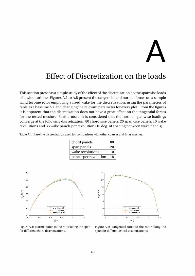
AEffect of Discretization on the loads

This section presents a simple study of the effect of the discretization on the spanwise loadsof a wind turbine. Figures A.1 to A.8 present the tangential and normal forces on a samplewind turbine rotor employing a fixed wake for the discretization, using the parameters oftable as a baseline A.1 and changing the relevant parameter for every plot. From the figuresit is apparent that the discretization does not have a great effect on the tangential forcesfor the tested meshes. Furthermore, it is considered that the normal spanwise loadingsconverge at the following discretization: 80 chordwise panels, 20 spanwise panels, 10 wakerevolutions and 36 wake panels per revolution (10 deg. of spacing between wake panels).

Table A.1: Baseline discretization used for comparison with other coarser and finer meshes.

chord panels 80span panels 20wake revolutions 10panels per revolution 18

Figure A.1: Normal force to the rotor along the spanfor different chord discretizations.

Figure A.2: Tangential force to the rotor along thespan for different chord discretizations.

43

44 A. Effect of Discretization on the loads

Figure A.3: Normal force to the rotor along the spanfor different spanwise discretizations.

Figure A.4: Tangential force to the rotor along thespan for different spanwise discretizations.

Figure A.5: Normal force to the rotor along the spanfor different number of wake revolutions.

Figure A.6: Tangential force to the rotor along thespan for different number of wake revolutions.

Figure A.7: Normal force to the rotor along the spanfor different number of wake panels per revolution.

Figure A.8: Normal force to the rotor along the spanfor different number of wake panels per revolution.

BFinite Difference checks

A finite difference check has been done to ensure that the analytical sensitivities are prop-erly calculated. The way this check works is the following: the value of the objectives andconstraints is calculated using the developed aerodynamic model (which has been previ-ously validated) for a specific blade geometry; then the variables are perturbed by a givenincrement ∆ρ such that the derivative of the objective can be approximated using expres-sion B.1 — similarly for the constraint function and its derivatives.

d f

dρ≈ ∆ f

∆ρ(B.1)

A finite difference scheme to calculate sensitivities is accurate for a specific step size,but becomes inaccurate when the step is too low (due to machine accuracy) and when thestep is too high (because the approximation of equation B.1 does not hold). The error of a fi-nite difference scheme plotted against the∆ρ perturbation then follows a characteristic ’V’shape. More insights into finite difference calculation can be seeked in Martins and Ning[2021]. Then, assuming that the sensitivities calculated using the analytic adjoint methodare correct, the difference between the adjoint sensitivities and the finite difference com-putations should resemble this ’V’ shape as well. This is what can be seen in figures B.1and B.2 for the objective and constraint sensitivities, respectively, of the fixed wake model.Every line corresponds to the mentioned relative error for a specific variable of the blade.In this case both the twist and the chord variables are shown for every section of the blade.The finite difference check ensures that the aerodynamic model and its derivatives coin-cide, but it is still necessary to ensure that the model itself is correct to be able to claim thatthe sensitivities point in the right direction.

45

46 B. Finite Difference checks

Figure B.1: Relative error between the finite differ-ence sensitivities and the adjoint sensitivities for theobjective function.

Figure B.2: Relative error between the finite differ-ence sensitivities and the adjoint sensitivities for theconstraint functions.

CCode structure and contribution

This thesis departs from previous work done in the ambit of optimization of aircraft wings(see Conlan-Smith [2020]). Therefore, at the start of this thesis work a software alreadyexisted that could analyze the loads on a wing and perform aerodynamic and aerostructuraloptimization. The additions that have been made to the software during this work can besummarized in the next points:

1. Geometry input

2. Rotational symmetry

• Influence coefficients and their derivatives

• Computation of the velocity field at the wake

3. Velocity field

• Source terms and their derivatives

• Load calculations and their derivatives

4. Wake modeling

• New wake geometry

• New scheme implemented with the Free-wake model

5. New objectives and constraints

47

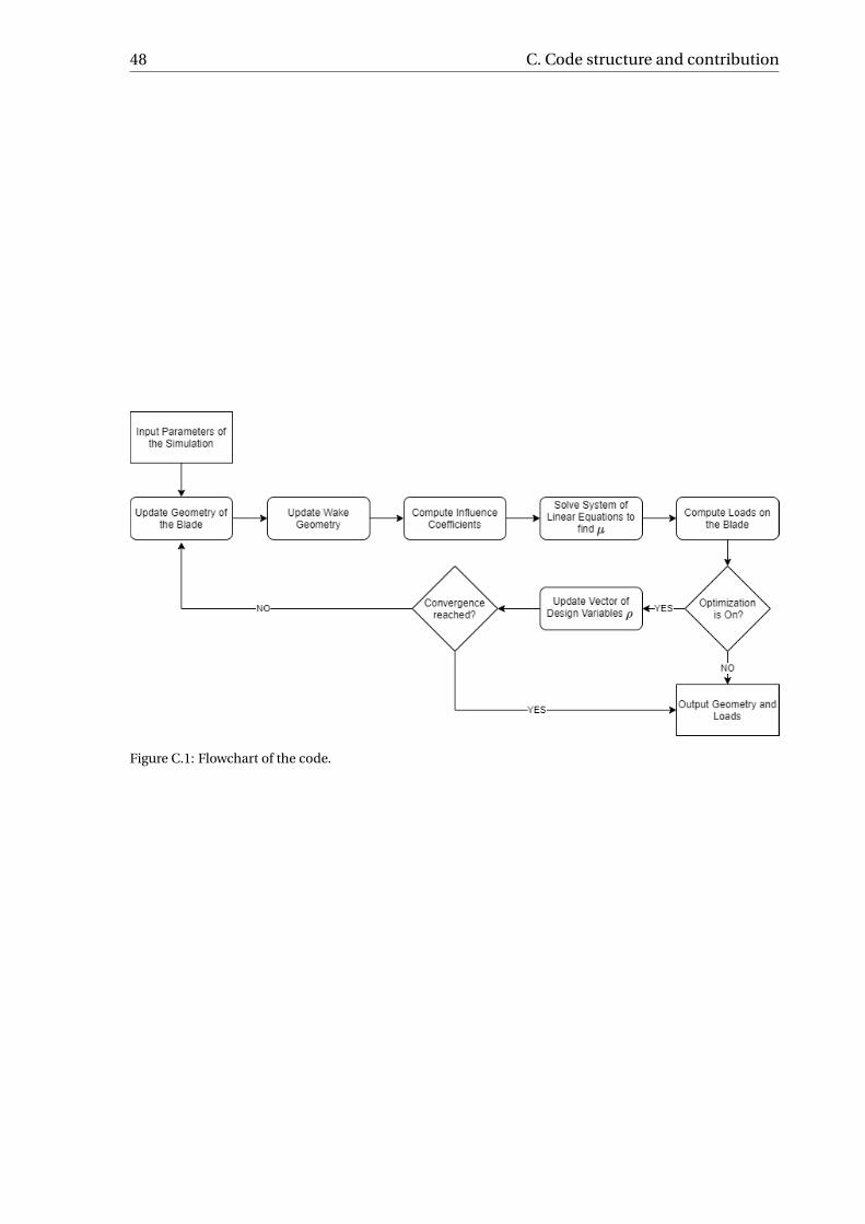
48 C. Code structure and contribution

Figure C.1: Flowchart of the code.

Bibliography

J. Anderson. Fundamentals of Aerodynamics, Sixth Edition. 2017.

T. Ashuri, M. B. Zaaijer, J. R.R.A. Martins, G. J.W. van Bussel, and G. A.M. van Kuik. Multidis-ciplinary design optimization of offshore wind turbines for minimum levelized cost ofenergy. Renewable Energy, 68, 2014. ISSN 09601481. doi: 10.1016/j.renene.2014.02.045.

F. Blondel, R. Boisard, M. Milekovic, G. Ferrer, C. Lienard, and D. Teixeira. Validationand comparison of aerodynamic modelling approaches for wind turbines. In Journalof Physics: Conference Series, volume 753, 2016. doi: 10.1088/1742-6596/753/2/022029.

C. L. Bottasso, A. Croce, L. Sartori, and F. Grasso. Free-form design of rotor blades. InJournal of Physics: Conference Series, volume 524, 2014. doi: 10.1088/1742-6596/524/1/012041.

C. L. Bottasso, P. Bortolotti, A. Croce, and F. Gualdoni. Integrated aero-structural optimiza-tion of wind turbines. Multibody System Dynamics, 38(4), 2016. ISSN 1573272X. doi:10.1007/s11044-015-9488-1.

Tony Burton, Nick Jenkins, David Sharpe, and Ervin Bossanyi. Wind Energy Handbook,Second Edition. 2011. doi: 10.1002/9781119992714.

C. Conlan-Smith, N. Ramos-García, O. Sigmund, and C. S. Andreasen. Aerodynamic ShapeOptimization of Aircraft Wings Using Panel Methods. AIAA Journal, 58(9):3765–3776, 92020. ISSN 0001-1452. doi: 10.2514/1.J058979. URL https://arc.aiaa.org/doi/10.2514/1.J058979.

Cian Conlan-Smith. Aerodynamic and Aeroelastic Shape Optimization of Aircraft Wings.PhD thesis, Technical University of Denmark, 2020.

Cian Conlan-Smith and Casper Schousboe Andreasen. A coupled 3D panel-beam modelfor aeroelastic optimization of aircraft wings. AIAA Journal, Accepted/In Press, 2020.

Mark Drela. Flight Vehicle Aerodynamics. 2014.

Gunter Reinald Fischer, Timoleon Kipouros, and Anthony Mark Savill. Multi-objective opti-misation of horizontal axis wind turbine structure and energy production using aerofoiland blade properties as design variables. Renewable Energy, 62:506–515, 2 2014. ISSN09601481. doi: 10.1016/j.renene.2013.08.009.

H. Glauert. Airplane Propellers. In Aerodynamic Theory. 1935. doi: 10.1007/978-3-642-91487-4\_3.

GWEC. Global Wind Report 2019. Technical report, 2020. URL https://gwec.net/global-wind-report-2019/.

49

https://arc.aiaa.org/doi/10.2514/1.J058979

https://arc.aiaa.org/doi/10.2514/1.J058979

https://gwec.net/global-wind-report-2019/

https://gwec.net/global-wind-report-2019/

50 Bibliography

M. O.L. Hansen, J. N. Sørensen, S. Voutsinas, N. Sørensen, and H. Aa Madsen. State of theart in wind turbine aerodynamics and aeroelasticity, 2006. ISSN 03760421.

Martin O.L. Hansen. Aerodynamics of wind turbines: Third edition. 2015. doi: 10.4324/9781315769981.

John L. Hess. Calculation of potential flow about arbitrary three dimensional lifting bodies.Technical report, McDonnell Douglas, 1973.

IEA. World Energy Outlook 2020. 2020. URL https://www.iea.org/reports/world-energy-outlook-2020#.

Kai A. James, Graeme J. Kennedy, and Joaquim R.R.A. Martins. Concurrent aerostruc-tural topology optimization of a wing box. Computers and Structures, 134, 2014. ISSN00457949. doi: 10.1016/j.compstruc.2013.12.007.

J. Jonkman, S. Butterfield, W. Musial, and G. Scott. Definition of a 5-MW reference windturbine for offshore system development. Contract, (February), 2009. ISSN 01487299.

J. Katz and A. Plotkin. Low-Speed Aerodynamics, Second Edition. Journal of Fluids Engi-neering, 126(2), 2004. ISSN 0098-2202. doi: 10.1115/1.1669432.

Gaetan K.W. Kenway, Graeme J. Kennedy, and Joaquim R.R.A. Martins. A CAD-free ap-proach to high-fidelity aerostructural optimization. In 13th AIAA/ISSMO Multidisci-plinary Analysis and Optimization Conference 2010, 2010. doi: 10.2514/6.2010-9231.

Stephen Lawton and Curran Crawford. Investigation and optimization of blade tip wingletsusing an implicit free wake vortex method. In Journal of Physics: Conference Series, vol-ume 524, 2014. doi: 10.1088/1742-6596/524/1/012033.

G. Leishman. Principles of helicopter aerodynamics. 2006.

R. M. Pinkerton. Calculated and measured pressure distributions over the midspan sectionof the NACA 4412 airfoil. Technical report, National Advisory Committee for Aeronautics,1937.

Mads H.Aa Madsen, Frederik Zahle, Niels N. Sørensen, and Joaquim R.R.A. Martins. Mul-tipoint high-fidelity CFD-based aerodynamic shape optimization of a 10 MW wind tur-bine. Wind Energy Science, 4(2), 2019. ISSN 23667451. doi: 10.5194/wes-4-163-2019.

Joaquim R.R.A Martins and Andrew Ning. Engineering Design Optimization. Working draftedition, 2021.

Bram Peerlings. A review of aerodynamic flow models, solution methods and solvers – andtheir applicability to aircraft conceptual design. Technical report, 2018.

N. Ramos-García, J. N. Sørensen, and W. Z. Shen. Validation of a three-dimensional viscous-inviscid interactive solver for wind turbine rotors. Renewable Energy, 70, 2014. ISSN09601481. doi: 10.1016/j.renene.2014.04.001.

https://www.iea.org/reports/world-energy-outlook-2020#

https://www.iea.org/reports/world-energy-outlook-2020#

Bibliography 51

D. J. Robison, F. N. Coton, R. A.Mc D. Galbraith, and M. Vezza. Application of a prescribedwake aerodynamic prediction scheme to horizontal axis wind turbines in axial flow.Wind Engineering, 19(1), 1995. ISSN 0309524X.

Matias Sessarego and Wen Zhong Shen. Aero-structural optimization of wind turbineblades using a reduced set of design load cases including turbulence. In Journal ofPhysics: Conference Series, volume 1037, 2018. doi: 10.1088/1742-6596/1037/4/042018.

Matias Sessarego, Néstor Ramos-García, Hua Yang, and Wen Zhong Shen. Aerodynamicwind-turbine rotor design using surrogate modeling and three-dimensional viscous-inviscid interaction technique. Renewable Energy, 93, 2016. ISSN 18790682. doi:10.1016/j.renene.2016.03.027.

Ole Sigmund. Morphology-based black and white filters for topology optimization. Struc-tural and Multidisciplinary Optimization, 33(4-5), 2007. ISSN 1615147X. doi: 10.1007/s00158-006-0087-x.

K. Svanberg. The method of moving asymptotes - a new method for structural optimiza-tion. International Journal for Numerical Methods in Engineering., 24(2), 1987.

Jesse Thé and Hesheng Yu. A critical review on the simulations of wind turbine aerodynam-ics focusing on hybrid RANS-LES methods, 2017. ISSN 03605442.

L.J. Vermeer, J.N. Sørensen, and A. Crespo. Wind turbine wake aerodynamics. Progress inAerospace Sciences, 39(6-7), 8 2003. ISSN 03760421. doi: 10.1016/S0376-0421(03)00078-2.

Júlio Xavier Vianna Neto, Elci José Guerra Junior, Sinvaldo Rodrigues Moreno, Helon Vi-cente Hultmann Ayala, Viviana Cocco Mariani, and Leandro dos Santos Coelho. Windturbine blade geometry design based on multi-objective optimization using metaheuris-tics. Energy, 162, 2018. ISSN 03605442. doi: 10.1016/j.energy.2018.07.186.

Tongguang Wang. A brief review on wind turbine aerodynamics. Theoretical and AppliedMechanics Letters, 2(6), 2012. ISSN 20950349. doi: 10.1063/2.1206201.

Zhijun Wang, Akke S.J. Suiker, Hèrm Hofmeyer, Twan van Hooff, and Bert Blocken. Coupledaerostructural shape and topology optimization of horizontal-axis wind turbine rotorblades. Energy Conversion and Management, 212, 2020. ISSN 01968904. doi: 10.1016/j.enconman.2020.112621.

Wind Europe. Wind energy in Europe in 2019. Technical report,2020. URL https://windeurope.org/data-and-analysis/product/wind-energy-in-europe-in-2019-trends-and-statistics/.

https://windeurope.org/data-and-analysis/product/wind-energy-in-europe-in-2019-trends-and-statistics/

https://windeurope.org/data-and-analysis/product/wind-energy-in-europe-in-2019-trends-and-statistics/

shape optimization of wind turbine blades using panel methods

Documents