shared datasets for imrt, beam angle optimization, and ... · craft et al. research shared datasets...

Craft et al.

RESEARCH

Shared datasets for IMRT, beam angleoptimization, and VMAT researchDavid Craft1*, Mark Bangert2, Troy Long3, David Papp1 and Jan Unkelbach1

*Correspondence:

[email protected] General Hospital,

Harvard Medical School, Boston,

MA

Full list of author information is

available at the end of the article†Equal contributor

Abstract

Background: We provide common datasets for researchers to use whendeveloping and contrasting radiation treatment planning optimization algorithms.The datasets allow researchers to make one-to-one comparisons of algorithms tosolve various instances of the radiation therapy treatment planning problem inintensity modulated radiation therapy (IMRT), including beam angleoptimization (BAO), volumetric modulated arc therapy (VMAT) and directaperture optimization (DAO).

Dataset: We provide datasets for a prostate case, a liver case, a head and neckcase, and a standard IMRT phantom. For each, we provide the dose-influencematrix from a variety of beam/couch angle pairs. The dose-influence matrix isthe main entity needed to perform optimizations: it contains the dose to eachpatient voxel from each pencil beam. We also provide the original DICOMcomputed tomography (CT) scan as well as the DICOM structure file.

Conclusions: We provide an open dataset – the first of its kind – to theradiation oncology community, which will allow researchers to compare methodsfor optimizing radiation dose delivery.

Keywords: IMRT; optimization; radiation therapy; beam angle optimization;VMAT; treatment plan optimization

BackgroundThe goal of radiation therapy for cancer treatment is to irradiate the tumorous

regions of the body with sufficiently high levels of radiation while sparing the nearby

healthy tissues as much as possible. In the mid 1990s a technique known as intensity

modulated radiation therapy (IMRT) emerged which allows for much more tailoring

of the 3D dose distribution inside the patient. Along with this extra freedom comes

the need for mathematical optimization, and over the last 20 years a large amount

of research has produced over of 600 papers revolving around this topic (this is

a conservative estimate based on a PubMed search for the words “IMRT” and

“optimization” in the title or abstract).

A deficiency in the field has been the lack of common datasets for researchers

to test their algorithms on. As such, most new algorithm papers simply state the

algorithm and demonstrate it, but the reader is left to wonder how this algorithm

compares with other approaches to the same problem. The raw data which was used

for a specific study is never provided as part of the publication. Reasons include

the data size, involvement of commercial software products, and protection of data

privacy for individual patients.

Craft et al. of 17

With this paper, we want to address these issues and provide the basis for mean-

ingful benchmarking of IMRT optimization algorithms. Specifically, our initiative

aims at resolving the following shortcomings:

• Patient cases used in different papers differ greatly in the geometry of their

targets and critical sturctures. A technique that works on an “easy” patient

may not work as well on a “hard” patient and vice versa.

• Research papers make different assumptions when deriving plan optimiza-

tion data from the patient’s planning CT. This includes the dose calculation

method, spatial resolution of the dose and beamlet grid, planning goals, deliv-

ery modality, etc. These data are generated in-house and are not shared with

the research community.

• New researchers in the field may not have access to clinical patient datasets.

The datasets we present herein are applicable to IMRT [1, 2, 3] and its variants,

including beam angle optimization (BAO) [4, 5, 6, 7], volumetric modulated arc

therapy (VMAT) [8, 9, 10, 11, 12, 13], 3D-conformal optimization [14, 15], stereo-

tactic body radiation therapy (SBRT) [16], and direct-aperture optimization (DAO)

[17, 18, 19, 20, 21, 22]. We refer the readers to the citations for explanations of each

of these (overlapping) modalities.

Data descriptionWe provide datasets for three anonymized cancer patient cases and one standard

IMRT phantom. For each of the four cases, we include the original DICOM CT

image as well as the DICOM RTStruct file containing the contours of targets and

organs at risk. These files are made available for viewing results, although they are

not necessary for optimization. In addition, the DICOM files give researchers to

opportunity to replan these patients in a commercial treatment planning system.

All further data is derived from the DICOM data.

Voxel grid

For dose calculation, the original CT image is downsampled to a lower resolution.

The final resolution and size of the dose grid in three dimensions is stored in a text

file named CTVOXEL INFO.txt. Each voxel in the 3D dose grid is assigned a voxel

index, which is used in optimization data described below. The coordinate system

and the conversion of voxel indices to spatial location is described in Appendix

A. For standard optimizations, voxel positions are not needed. They are however

needed for visualization of the dose distribution, and are useful for implementing

objective functions which require spatial information, for example a dose penalty

which depends on the distance from a normal tissue voxel to the patient’s tumor.

This file also contains the isocenter location. The isocenter is the common point

that all the beams pass through.

Beamlet grid

The incident fluence is discretized into a rectangular grid of beamlets. We use a

beamlet size of 1 cm by 1 cm for all cases except for the head and neck case, for

which we use 0.5 cm by 0.5 cm. The isocenter is identical for all beam directions and

is located in the center of mass of the union of all target volumes. The set of beamlets

Craft et al. of 17

for which dose is calculated is based on an isotropic 2.5 mm expansion of the union

of all targets. A beamlet is included in the fluence map if its central axis intesects

the enlarged target. In a post-processing step, we ensure that the beamlet grid is

consecutive. If beamlets are missing from the fluence map, causing a hole across an

MLC row, these beamlets are added and their dose distribution is calculated. This

issue arises for example in the head and neck case with disconnected targets on either

side of the neck. Missing beamlets could be problematic for sliding window IMRT

and VMAT optimization approaches, where the MLC leaves would potentially slide

over those beamlets. The beamlet grid coordinate system is described in Appendix

A

Optimization data

All binary formatted data are saved from Matlab as *.mat files (we have used

Matlab version 7.14.0.739, R2012a)[1]. In this way, data can either be read into

Matlab, Octave, or Python using the scipy package. Instructions for reading in the

data are given in the Methods section. For treatment plan optimization, we provide

the following files for each patient.

Voxel lists

The voxel list files contain the voxel indices of the voxels which are inside each

geometrically contoured structure. The information is stored as a list of integers in

the files {structure name} VOILIST.mat. The format thus allows for overlapping

structures, i.e. a given voxel index can be contained in multiple voxel lists.

Beamlet information

For each (gantry angle, couch angle) pair, a beam info file with the file name

Gantry{gantry angle} Couch{couch angle} BEAMINFO.mat is provided. The file

contains the following information:

• couch angle

• gantry angle

• number of beamlets

• number of non-zeros in the dose-influence matrix (see next section; this value

is helpful for pre-allocating memory to store these matrices)

• A vector of the x position of each of the beamlets (using the gantry head

coordinate system, see figure 3).

• A vector of the y position of each of the beamlets (see figure 3).

Geometric beamlet information is not necessary for the most basic type of IMRT

optimization, but for VMAT, and DAO (where “apertures” are created by combin-

ing adjacent beamlets), it is necessary to know the geometric location of each of the

beamlets.

[1]Note that, if one were to use a more recent version of Matlab to save data for

reading into Python etc, one should use the Matlab toggle -v7 during the save

command.

Craft et al. of 17

Dose-influence matrix

The dose influence matrix Dij is the main entity used for optimization. It contains

the dose delivered to each voxel i per unit intensity of beamlet j. We provide

the dose influence matrix in units of Gray per monitor unit (Gy/MU) [2]. The

dose-influence matrix is stored in seperate files for each (gantry angle, couch angle)

pair in files named Gantry{gantry angle} Couch{couch angle} D.mat. Each of these

files contains a single matrix called D, which is a Matlab sparse matrix [3]. We use

CERR version 4.4 (Computational Environment for Radiotherapy Research) [23] to

produce the dose influence matrices for each case. CERR uses a pencil beam type

dose calculation algorithm referred to as the quadrant infinite beam (QIB) model

[24].

The dose to voxel i is given by di =∑

j Dijxj where xj is the fluence value of the

jth beamlet.

Hints for CERR users

To generate the optimization data, the dicom CT data was imported into CERR and

the CT scan was then resampled to the voxel sizes shown in Table 1. This was done

using the CERR command downSampleScan. Once the data was downsampled, the

CERR IMRTP module was used to create the dose-influence matrices. Our group

has modified this code to allow for couch rotations. The dose-influence matrix was

then extracted from the internal CERR data structure and rescaled to units of

Gy/MU. We also provide a Matlab .mat which is generated by CERR when saving

the patient. This file contains, among other attributes, the downsampled CT scan,

which has the same resolution as the dose grid, and can be used for visualization.

For size purposes, this file does not contain the Dij matrices.

The four cases

We provide data sets for four patients of different sizes to support a variety of

radiotherapy planning problems and represent typical treatment sites. The main

characteristics of all datasets are summarized in Table 1. A representative transver-

sal slice through the CT, illustrating the geometry of target and OARs for each

case, is shown in figure 1.

TG119 dataset

The first case we use is a phantom provided by the American Association of Physi-

cists in Medicine Task Group 119 for use in institutional IMRT commissioning

(i.e. readying a clinic for IMRT treatments) [25]. This phantom has several sets

of contours for various IMRT treatment planning tests, but we only use three of

the contours: a C-shaped target (called “OuterTarget”), an OAR that the target

[2]The unit of beamlet intensity (MU) is defined such that 100 MU yields a dose of

1 Gy in 10 cm depth in water in the center of a 10 cm by 10 cm radiation field.[3]The dose influence matrix can by read directly into Matlab, Octave and Python

as a sparse matrix (see the Methods section). Note however that Python is 0-based

whereas Matlab and Octave are 1-based. The voxels indices stored in the {structure

name} VOILIST.mat files are 1-based, i.e., the lowest voxel index is 1, as depicted

in figure 2. Thus the user has to perform the appropriate shift when using Python.

Craft et al. of 17

wraps around (“Core”), and the external contour of the phantom itself (“BODY”).

For this case we provide five equispaced coplanar beams (coplanar refers to beams

where the couch angle is fixed at 0◦) at gantry angles 0◦, 72◦, 144◦, 216◦, and 288◦.

This serves as our small dataset. The total number of beamlets at each respective

angle is 98, 70, 90, 90 and 70, for a total of 418 beamlets.

TG119 Prostate Liver Head and neckNumber of beam angles 5 180 56 1983Total number of beamlets 418 25,404 3678 2,257,507Noncoplanar no no yes yesBeamlet size [cm] 1x1 1x1 1x1 0.5x0.5Voxel resolution (LR,AP,SI) [mm] (3.0, 3.0, 2.5) (3.0, 3.0, 3.0) (3.0, 3.0, 2.5) (3.0, 3.0, 5.0)Voxel grid size (LR,AP,SI) (167,167,129) (184,184,90) (217, 217,168) (160,160,167)Number of target voxels 7429 9491 6954 25,388Number of voxels in patient 599,440 690,373 1,927,357 251,893dataset size 25 MB 1.9 GB 560 MB 64 GB

Table 1: Summary of Patient characteristics. Number of target voxels for the head and

neck case is for the union of the three PTV structures.

Prostate

The prostate case serves as one of our two medium size datasets. We generate

180 equispaced coplanar beams, thus this data set serves as a test case for VMAT

algorithms. Using a beamlet resolution of 1cm×1cm, the total number of beamlets

is 25,404. There are two targets for the prostate case. The highest prescription dose

target, PTV 68, is a geometric expansion of the prostate. The lower dose target,

PTV 56, is an expansion around the prostate and the lymph nodes.

SBRT liver case

This is the first non-coplanar case we present. We originally generate 162 (gantry,

couch) angle pairs such that the entry angles are evenly scattered over a sphere

corresponding to an average angular spacing of 16◦. This was done using a Matlab

routine called GridSphere available from the File Exchange portion of the Math-

Works website. We then eliminate beams that have either entrance or exit doses

through the first slice of the CT since if this is the case, the full dose deposit of the

beam is not properly accounted for. This leaves 56 beams in the dataset, with a

total of 3678. Note that given a particular linac, some gantry/counch angle combi-

nations may not be allowed due to mechanical collisions. Since this is linac specific,

we have not attempted to eliminate such beams, and instead leave it to the reader

to keep this in mind if modeling an actual clinical delivery situation.

Head and neck

This serves as our large dataset. The CT and structures are obtained from the pub-

lically available research set www.cancerimagingarchive.net. This set was created

with non-coplanar VMAT in mind and creates a full set of equispaced beams for a

variety of couch angles. The couch angles are -90◦ to 90◦ in increments of 5◦. At the

couch angles -90, 0, and 90, we place beams at a 2◦ gantry spacing. At the other

couch angles we use a 5◦ gantry spacing. 2◦ resolution is the clinical standard gantry

discretization for computing VMAT doses; 5◦ is adequate for research purposes. We

eliminate beams that enter through the inferior most CT slice, where the CT scan

Craft et al. of 17

ends. The elimination map is shown in Figure 4. This leaves 1983 beam angles used,

with a total of 2,257,507 beamlets. The beamlets for this case are 0.5cm×0.5cm.

the voxel resolution is 3mm×3mm×5mm. Unfortunately we cannot provide data at

a higher resolution in the sup-inf direction due the sparse resolution of 5mm in the

original CT. Still, this is perfectly adequate for computation research purposes.

OuterTarget

Core

BODY

TG119 Prostate

Liver Head and Neck

Rectum

Lt femoral head

Bladder

Rt femoral head

PTV_68

PTV_56

BODY

Liver

Skin

Stomach

SpinalCord

CTVPTV

PTV_63

PTV_70

SpinalCord PRV

ParotidRt

ParotidLt

Figure 1 Axial views of the four cases CT and structures for the four cases for a representativeCT slice (which shows some but not all of the structures included in the dataset).

AnalysesAs a data verification step, we give dose distribution statistics for the ones solutions

(xj = 1 for all j) for all cases. We give the dose statistics for two volumes from each

case, one target and one critical structure, see Table 2. In the Methods section we

provide the Matlab code used to perform this calculation.

Case Structure name minimum dose mean dose maximum dose

TG119 Core 0.026798 0.050724 0.053313OuterTarget 0.049379 0.051067 0.052702

Prostate PTV 56 1.3015 1.3631 1.4089Bladder 0.66549 1.2753 1.3863

Liver Heart 0.0003963 0.093117 0.4388PTV 0.37532 0.41629 0.48094

Head and Neck PTV 70 19.5394 21.0998 23.1338PAROTID LT 8.7997 20.3354 23.7127

Table 2: Dose statistics for all cases, for two selected structures, for the ones solution

(all beams), i.e. di =∑

j Dij. This serves as a data consistency check for users.

Craft et al. of 17

Optimization demonstration and results

Description of the IMRT optimization problem

Here we describe what is known as the fluence-based IMRT optimization problem.

This an idealized version of the actual IMRT treatment planning problem, but

is commonly used to develop algorithms and indeed is possible to use in clinical

settings (e.g. [26]).

For a set of beams, we assume the D matrix represents the entire set of beamlets

from all the beams. That is, below D is interpreted as a concatenation of the

individual D matrices from each beam. This notationally simplifies the problem,

allowing us to avoid looping over the beams, instead we just loop over all beamlets.

Let d be the vector of voxel doses, and let x be the vector of beamlet fluences. The

key mapping is the linear relationship between the beamlet vector and the dose

distribution and is given by d = Dx, where matrix-vector multiplication is used

as shorthand for di =∑

j Dijxj . Writing this dose calculation in the form of a

matrix-vector product, a generic formulation of the IMRT optimization prolem is

as follows:

minimize f(d)

Dx = d

d ∈ C

x ≥ 0, (1)

A specific example that would give rise to a linear program would be to choose as

f(d) the mean dose to a critical structure, and to invoke upper bounds for all voxels

and additional lower bounds for the target voxels via the constraint set C. A typical

quadratic formulation would set goals for every voxel (for example, prescription dose

to all target voxels and 0 to all other voxels) and minimize the squared deviation

from those levels.

BAO, DAO, and VMAT formulations put additional restrictions on the x vec-

tor. For example for BAO, one might restrict that a total of 5 beams are used at

most, and thus integer variables could be added to this formulation to control the

maximum number of active beams/beamlets.

Examples of linear programming formulations

Here we present simple linear programming formulations and summary results for

each of the four cases. These formulations are not meant to produce quality treat-

ment plans but are rather selected to be simple to implement and thus reproduce

results as a baseline.

Objective min (mean Core + mean BODY)Constraints OuterTarget >= 1

OuterTarget <=1.2Core <=1.2

Results mean Core = 0.2489mean BODY = 0.1021

Table 3: Linear programming formulation and solution statistics for the TG119 case,

all five beams used.

Craft et al. of 17

Objective min (mean Rectum + 0.6*mean Bladder+ 0.6*mean BODY)Constraints PTV 68 >= 1

x <=50Results mean Rectum = 0.2842

mean Bladder = 0.4035mean BODY = 0.0905

Table 4: Linear programming formulation and solution statistics for the Prostate case,

using the five beams at gantry angles 0◦, 72◦, 144◦, 216◦, and 288◦.

Objective min (mean Liver + mean Heart+ 0.6*mean entrance)Constraints PTV >= 1

x <=25Results mean Liver = 0.1771

mean Heart = 0.1258mean Entrance = 0.0186

Table 5: Linear programming formulation and solution statistics for the Liver case, using

the seven beams at (gantry, couch) angles (58◦, 0◦), (106◦, 0◦), (212◦, 0◦), (328◦, 0◦),

(216◦, 32◦), (226◦, -13◦), (296◦, 17◦).

Objective min (mean Left Parotid + mean Right ParotidConstraints All PTVs >= 1

spinal cord <=0.5brainstem <=0.5x <=25

Results mean Left Parotid = 0.4959mean Right Parotid = 0.3437

Table 6: Linear programming formulation and solution statistics for the Head and Neck

case, using five gantry angles at couch=0◦ (0◦, 72◦, 144◦, 216◦, and 288◦) as well as

five gantry angles at couch=20◦ (180◦, 220◦, 260◦, 300◦, 340◦).

DiscussionWe provide four datasets for radiotherapy treatment plan optimization. The

datasets are meant to serve several purposes:

• We provide datasets for reasearchers in the optimization community who may

not have access to patient data.

• Advanced problems like BAO, DAO, and VMAT represent non-convex or com-

binatorial problems which typically cannot be solved to optimality. Thus, so-

lution approaches are heuristics, and different methods can only be compared

meaningfully based on common datasets, where differences due to patient

geometry and dose calculation are eliminated.

• The datasets can serve as benchmark cases for the development of fast and

efficient solvers customized to fluence map optimization and its variants. This

development may also benefit other radiotherapy planning problems such as

robust optimization in proton therapy and adaptive replanning in online im-

age guided radiotherapy. Our datasets do not per se support these specific

problems. However, such applications rely on very fast optimization methods

that can handle large data.

Solution reporting

We recommend that researchers share results in the maximally transparent and

reproducible manner. This includes the statement of the full optimization problem

Craft et al. of 17

that was solved. In addition, the solution should be shared in the form of fluence

maps, from which the dose distribution and all dose measures can be derived. The

details of the solution reporting may depend on the application:

• For IMRT fluence map optimization, the solution is the vector of beamlet

intensities x at each beam (gantry/couch pair) that is used in the solution.

As such, we recommend the following file format for users to report and share

solutions. The file name should match the name of the Dij file (replacing the

“ D.mat” with “ beamletSol.mat”), and should consist of fluence values stored

as a vector called beamx. The beamlet solution files for the linear programs

solved above are included in the data download.

• For DAO applications, the solution can be reported through an effective flu-

ence map for each individual aperture, using the same format. Similarly,

VMAT algorithms that represent extensions of DAO algorithms can report

the solution in the form of effective fluence maps for all control points.

Fluence map optimization

We have presented results for the ones solutions and for simple linear programs for

the purpose of data testing and consistency. We have not included solution times

since the purpose of this paper is not to present methods for fast/quality solutions

to the IMRT problem, but rather to provide a set of data for the community to do

such things. We used the Matlab linear programming solver (linprog) to solve the

TG119, the prostate, and the liver case, but switched to CPLEX’s Matlab interface

(cplexlp) to solve the head and neck case, due to its size. All cases finished in under

two minutes, except for the head and neck case which took about 8 minutes.

The optimization formulation given in formulation 1 involves a linear mapping

from the fluence values x to the voxel doses d. As such, provided the function f(d)

is convex and the constraint set C is convex, the problem is a convex optimization

problem. Real world constraints often make the problem non-convex however (a

non-convex objective would as well, although that seems less fundamental: there

is no work that proves that non-convex objective functions are needed to produce

high quality treatment plans). The discrete form of the beam angle optimization

problem, where candidate beams are pre-selected and the optimization problem is

to find a subset of the beams (for example, the seven best beams) and their beamlet

fluences to optimize a given objective, is a combinatorial problem.

DAO and VMAT applications

In modern clinical treatment planning systems, fluence based optimization is done

(at most) as an initial step. Final plan optimization involves determining aperture

shapes (specified by the positions of MLC leaves) and weights. To than end, many

modern planning systems apply DAO methods. Once a segment shape is computed,

the dose is linear in the segment weight. To a first approximation, the dose contri-

bution from a segment is the sum of the contributions from the individual beamlets

that constitute that segment, i.e. the information stored in the Dij matrix. But bet-

ter accuracy is obtained by doing a dose computation for each individual aperture

shape, which involves scatter terms that can only be computed once the aperture

shape is known. Using the datasets provided herein, dose calculation for an aper-

ture is limited to approximations based on the Dij matrix. Despite this limitation,

Craft et al. of 17

this dataset can be used for DAO algorithm design. Indeed, most DAO algorithms

heavily utilize the Dij matrix concept for generating promising apertures [22] or for

approximating gradients with respect to MLC leaf positions [27, 20]. Only a more

accurate final or intermittent recalculation of an aperture’s dose distribution cannot

be performed using this dataset.

Similarly, VMAT treatments need to consider MLC leaf positions in order to

emulate a clinical VMAT optimizer. VMAT solvers typically strive to find a solution

where the beam rotates completely around the patient on the order of minutes. As

such, complete fluence modulation cannot be achieved at every angle, and MLC leaf

positions must be tracked to make sure neighboring apertures are similar so that

the gantry does not need to slow down excessively to move the leaves far across

the treatment field. Because this dataset involves beamlet position information and

couch and gantry positions, it can be used for VMAT optimization research. To

include delivery time in VMAT planning optimization one must specify a dose rate.

A typical value is 600 MU/min.

ConclusionWe provide the first open dataset to the radiation oncology community, thus allow-

ing researchers to compare methods for optimizing radiation dose delivery. The

dataset comprises four patient cases from different sites. Besides CT data and

structure sets, we also include dose calculation data in order to enable a one-to-

one comparison of novel and existing optimization strategies for intensity mod-

ulated radiation therapy, beam angle optimization, direct aperture optimization,

and volumetric-modulated arc therapy.

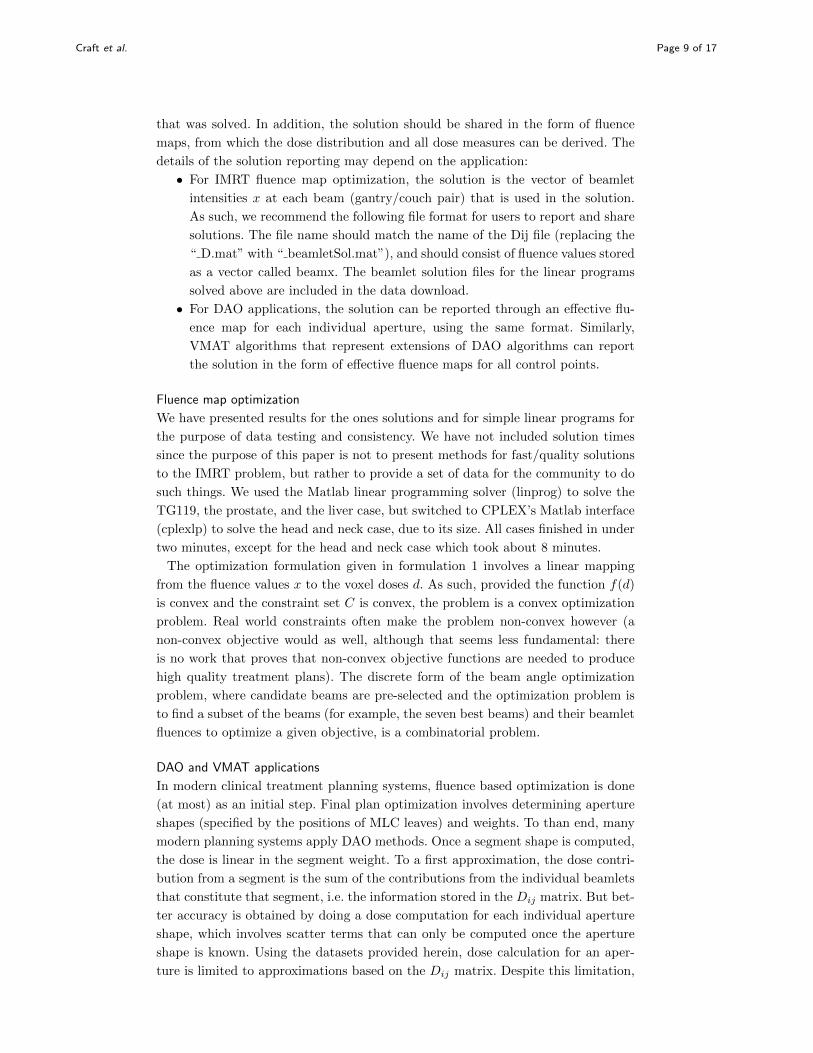
Appendix A: Coordinate systemsFigure 2 shows the conversion from voxel indices to voxel locations inside the pa-

tient. All patients in the data set are in standard orientation, i.e. supine and head

first. The voxel with index ”1” is located most anterior, superior, and to the pa-

tient’s right. For voxel indexing, the anterior-posterior direction corresponds to the

fastest changing index; the superior-inferior direction corresponds to the slowest

changing index.

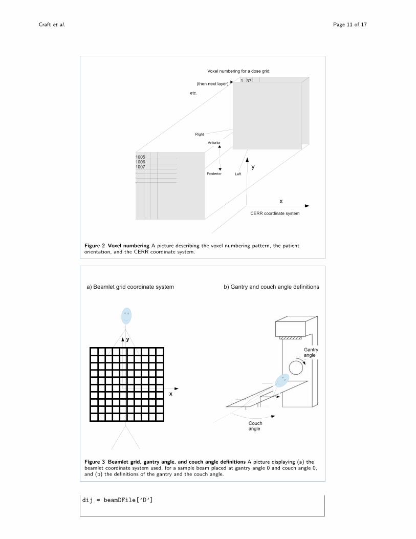
Figure 3(a) shows the definition of the beamlet grid. Throughout the dataset we

assume a collimator angle of 0. For a couch angle of 0, the y-axis of the beamlet

grid corresponds to the superior-inferior direction of the patient. For a gantry angle

of 0, the x-axis of the beamlet grid corresponds to the left-right direction of the

patient. Figure 3(b) shows the definition of the positive gantry and couch angles.

Appendix B: Demonstration codeFor reading data into Python, the scipy package is used, and then the Matlab .mat

files can be read directly. For example:

import scipy.io as io

beamDFile = io.loadmat(’Gantry0_Couch0_D.mat’)

Craft et al. of 17

z

y

x

123456etc

373839..

100510061007...

Voxel numbering for a dose grid:

CERR coordinate system

Right

Left

Anterior

Posterior

(then next layer)

etc.

Figure 2 Voxel numbering A picture describing the voxel numbering pattern, the patientorientation, and the CERR coordinate system.

x

y

a) Beamlet grid coordinate system

Couch angle

Gantry angle

b) Gantry and couch angle definitions

Figure 3 Beamlet grid, gantry angle, and couch angle definitions A picture displaying (a) thebeamlet coordinate system used, for a sample beam placed at gantry angle 0 and couch angle 0,and (b) the definitions of the gantry and the couch angle.

dij = beamDFile[’D’]

Craft et al. of 17

Next we include two sample code snippets to assist people in getting started with

the datasets in the Matlab environment. First we give a code which computes the

mean dose to a structure for the ones solution of all of the beams in the current

working directory.

beamdir = ’./’;

allFiles = dir([beamdir ’*D.mat’]);

allNames = { allFiles.name };

d = [];

for i=1:length(allNames)

f = allNames{i};

%load the matrix D for the gantry/couch pair

%stored in the file f:

load(f)

[nv, nb]=size(D);

if i==1

d = D*ones(nb,1);

else

d = d + D*ones(nb,1);

end

end

fname = ’OuterTarget_VOILIST.mat’;

%load a vector v of the voxel indices:

load(fname)

%get dose distribution for just those voxels:

dstruct = d(v);

%compute and display dose stats

dmin = min(dstruct);

dmean = mean(dstruct);

dmax = max(dstruct);

disp([’min, mean, max = ’ num2str(dmin) ’, ’ ...

num2str(dmean) ’, ’ num2str(dmax)]);

Next we give the code for obtaining a simple linear programming solution for the

liver case. The first section of the matlab code reads the dose-influence matrix for

7 selected beam angles and constructs the concatenated Dij matrix. Subsequently,

the voxel lists for 5 of the structures are imported.

%Gantry and couch angles to use:

ga = [58 106 212 328 216 226 296];

Craft et al. of 17

ca = [0 0 0 0 32 -13 17];

Dij = 0;

%Form the Dij matrix

for i=1:length(ga)

fname = [’Gantry’ num2str(ga(i)) ’_Couch’ num2str(ca(i)) ’_D.mat’];

load(fname)

%number of beamlets at angle i

nba(i) = size(D,2);

if i==1

Dij = D;

else

Dij = [Dij D];

end

end

%Load structures

load(’PTV_VOILIST.mat’);

V{1} = v;

load(’Liver_VOILIST.mat’);

V{2} = v;

load(’Heart_VOILIST.mat’);

V{3} = v;

load(’entrance_VOILIST.mat’);

V{4} = v;

load(’Skin_VOILIST.mat’);

V{5} = v;

The next code section constructs a linear optimization problem as described in

section . A weighted sum of the mean doses to the liver, the heart, and the normal

tissue in the entrance region is minimized, subject to the constraints that every PTV

voxel receives a dose larger than one. The linear program is solved using Matlab’s

build-in solver linprog. The optimal fluence map is returned into the vector x.

% mean doses contributions of all beamlets

Dlivermean = mean(Dij(V{2},:));

Dheartmean = mean(Dij(V{3},:));

Dentrancemean = mean(Dij(V{4},:));

%construct the linear inequality constraints

%to enforce a minimum dose of 1 to the PTV

A = -Dij(V{1},:);

Craft et al. of 17

b = -1*ones(size(A,1),1);

%cost vector

c = Dlivermean + Dheartmean + 0.6*Dentrancemean;

%bounds in beamlet intensity

nb = size(Dij,2); % total number of beamlets

lb = zeros(nb,1); % lower bound of zero

ub = 25*ones(nb,1); % upper bound of 25 MU

%optimization options

opt = optimset(’Display’,’iter’);

opt.LargeScale = ’on’;

%solve problem using matlab’s LP solver

[x, fval, eflag] = linprog(c,A,b,[],[],lb,ub,[],opt);

Next, the solution to the fluence map optimization problem is saved in the rec-

ommended format:

%save solution in our recommended format

ctr = 1;

for i=1:length(ga)

fname = [’Gantry’ num2str(ga(i)) ’_Couch’ ...

num2str(ca(i)) ’_beamletSol.mat’];

%num beamlets at angle i = nba(i)

beamx = x(ctr:ctr+nba(i)-1);

save(fname,’beamx’);

ctr = ctr+nba(i);

end

Finally, the mean doses are reported and the 3D dose distribution is visualized.

The vector of dose values is obtained by multiplying the dose influence matrix

with the beamlet intensity vector. The dose vector is then converted into a 3D

dose distribution based on the voxel numbering pattern described in appendix A.

The voxel lists for the structures are converted to 3D binary masks and plotted

as contours on top of the colorwash dose display. CERR users can use the CERR

function showIMDose.

%report mean doses to structs:

Dlivermean*x

Dheartmean*x

Dentrancemean*x

%calculate dose distribution

d = Dij*x;

%reshape dose vector to 3-dimensional array

Craft et al. of 17

%dose grid dimensions

dim = [217 217 168];

%total number of voxels

nVoxels = 217*217*168;

%reshape dose vector

dose = reshape(d,dim);

%create 3-dimensional masks for structures

for(s=1:length(V))

mask{s} = zeros(nVoxels,1);

for(i=1:length(V{s}))

mask{s}(V{s}(i))=1;

end

mask{s} = reshape(mask{s},dim);

end

%select axial slice to plot

slice = 50;

%plot dose and structures

figure;

set(gca,’DataAspectRatio’,[1 1 1]);

set(gca,’YDir’,’rev’);

axis([30 190 40 160]);

hold on;

%plot colorwash dose

imagesc(dose(:,:,slice));

%plot contours for PTV, Liver, Skin

for(s=[1 2 5])

contour(mask{s}(:,:,slice),[0.5],’k’,’LineWidth’,2);

end

hold off;

Competing interestsThe authors declare that they have no competing interests.

Authors’ contributionsDC carried out the overall project concept, the data generation, and the writing. DP modified CERR to be able to

compute noncoplanar beams, and also tested the datasets. TL, MB and JU contributed to writing the manuscript

and testing the datasets. Everyone proofread the manuscript.

Author details1Massachusetts General Hospital, Harvard Medical School, Boston, MA. 2German Cancer Research Center

(DKFZ), Heidelberg, Germany. 3University of Michigan, Ann Arbor, Michigan.

References1. Alber, M., Nusslin, F.: Intensity modulated photon beams subject to a minimal surface constraint. Physics in

Medicine and Biology 45, 49–52 (2000)

2. Oelfke, U., Bortfeld, T.: Inverse planning for photon and proton beams. Med. Dosim. 26, 113–124 (2001)

3. Webb, S.: A simple method to control aspects of fluence modulation in IMRT planning. Physics in Medicine

and Biology 46, 187–195 (2001)

Craft et al. of 17

4. Bangert, M., Ziegenhein, P., Oelfke, U.: Characterizing the combinatorial beam angle selection problem.

Physics in Medicine and Biology 57(20), 6707 (2012)

5. Wang, X., Zhang, X., Dong, L., Liu, H., Wu, Q., R., M.: Development of methods for beam angle optimization

for IMRT using an accelerated exhaustive search strategy. Int. J. Radiation Oncology Biol. Phys. 60(4),

1325–37 (2004)

6. Craft, D.: Local beam angle optimization with linear programming and gradient search. Physics in Medicine

and Biology 52(7), 127–135 (2007)

7. Breedveld, S., Storchi, P., Voet, P., Heijmen, B.: iCycle: integrated, multicriterial beam angle, and profile

optimization for generation of coplanar and noncoplanar IMRT plans. Medical Physics 39, 951 (2012)

8. Yu, C., Tang, G.: Intensity-modulated arc therapy: principles, technologies and clinical implementation. Physics

in Medicine and Biology 56(5), 31–54 (2011)

9. Craft, D., McQuaid, D., Wala, J., Chen, W., Salari, E., Bortfeld, T.: Multicriteria VMAT optimization. Medical

Physics 39, 686 (2012)

10. Bokrantz, R.: Multicriteria optimization for volumetric-modulated arc therapy by decomposition into a

fluence-based relaxation and a segment weight-based restriction. Medical Physics 39, 6712 (2012)

11. Papp, D., Unkelbach, J.: Direct leaf trajectory optimization for volumetric modulated arc therapy planning with

sliding window delivery. Submitted 53(4), 985–998 (2013)

12. Otto, K.: Volumetric modulated arc therapy: IMRT in a single gantry arc. Medical physics 35, 310 (2008)

13. Bzdusek, K., Friberger, H., Eriksson, K., Hardemark, B., Robinson, D., Kaus, M.: Development and evaluation

of an efficient approach to volumetric arc therapy planning. Medical physics 36, 2328 (2009)

14. Meng, B., Zhu, L., Widrow, B., Boyd, S., Xing, L.: A unified framework for 3D radiation therapy and IMRT

planning: plan optimization in the beamlet domain by constraining or regularizing the fluence map variations.


15. Khan, F., Craft, D.: 3d conformal planning using low segment multi-criteria imrt optimization. arXiv 100(100),

100 (2014)

16. Yarmand, H., Winey, B., Craft, D.: Guaranteed epsilon-optimal treatment plans with the minimum number of

beams for stereotactic body radiation therapy. Physics in Medicine and Biology 58(17), 5931 (2013)

17. Salari, E., Unkelbach, J.: A column-generation-based method for multi-criteria direct aperture optimization.


18. Shepard, D., Earl, M., Li, X., Naqvi, S., Yu, C.: Direct aperture optimization: A turnkey solution for

step-and-shoot IMRT. Medical Physics 29, 1007–1018 (2002)

19. Men, C., Romeijn, H., Taskın, Z., Dempsey, J.: An exact approach to direct aperture optimization in IMRT

treatment planning. Physics in Medicine and Biology 52, 7333 (2007)

20. Cassioli, A., Unkelbach, J.: Aperture shape optimization for IMRT treatment planning. Physics in Medicine and

Biology 58(2), 301 (2013)

21. Carlsson, F.: Combining segment generation with direct step-and-shoot optimization in intensity-modulated

radiation therapy. Medical physics 35, 3828 (2008)

22. Romeijn, H.E., Ahuja, R.K., Dempsey, J.F., Kumar, A.: A column generation approach to radiation therapy

treatment planning using aperture modulation. SIAM Journal on Optimization 15(3), 838–862 (2005)

23. Deasy, J., Blanco, A., Clark, V.: Cerr: A computational environment for radiotherapy research. Medical Physics

30(5), 979–985 (2003)

24. Kalinin, E., Deasy, J.: A method for fast 3-D IMRT dose calculations: The quadrant infinite beam (QIB)

algorithm. In: Medical Physics, vol. 30, pp. 1348–1349 (2003)

25. Ezzell, G., Burmeister, J., Dogan, N., LoSasso, T., Mechalakos, J., Mihailidis, D., Molineu, A., Palta, J.,

Ramsey, C., Salter, B.e.a.: IMRT commissioning: multiple institution planning and dosimetry comparisons, a

report from AAPM Task Group 119. Medical Physics 36(11), 5359–5373 (2009)

26. Jelen, U., Sohn, M., Alber, M.: A finite size pencil beam for IMRT dose optimization. Physics in Medicine and

Biology 50(8), 1747–1766 (2005)

27. Hardemark, B., Liander, A., Rehbinder, H., Lof, J.: Direct machine parameter optimization with RayMachine R©

in Pinnacle3 R©. RaySearch White Paper. Stockholm, Sweden: RaySearch Laboratories AB (2003)

Figures

Craft et al. of 17

avoid

avoid

For head and neck..avoid coming in though inferior CT slice

Figure 4 Elimination map for head and neck angles A picture displaying the couch/gantry anglepairs that were eliminated due to the beam entering the inferior CT slice, thus causing anincorrect dose computation.

shared datasets for imrt, beam angle optimization, and ... · craft et al. research shared datasets...

Documents