IEICE TRANS. FUNDAMENTALS, VOL. E00–A, NO. 1 JANUARY 20001

PAPER Surveys on Discovery Science

Expressive Tests for Classification and Regression∗∗

Shinichi Morishita† and Akihiro Nakaya†, Nonmembers

SUMMARY We address the problem of computing varioustypes of expressive tests for decision trees and regression trees.Using expressive tests is promising, because it may improve theprediction accuracy of trees, and it may also provide us somehints on scientific discovery. The drawback is that computingan optimal test could be costly. We present a unified frameworkto approach this problem, and we revisit the design of efficientalgorithms for computing important special cases. We also provethat it is intractable to compute an optimal conjunction or dis-junction.key words: classification, regression, decision trees

1. Introduction

A decision (resp. regression) tree is a rooted binary treestructure for predicting the categorical (numeric) val-ues of the objective attribute. Each internal node has atest on conditional attributes that splits data into twoclasses. A record is recursively tested at internal nodesand eventually reaches a leaf node. A good decision(resp. regression) tree has the property that almost allthe records arriving at every node take a single categor-ical value (a numeric value close to the average) of theobjective attribute with a high probability, and hencethe single value (the average) could be a good predictorof the objective attribute.

Making decision trees [9]–[11] and regression trees[2] has been a traditional research topic in the field ofmachine learning and artificial intelligence. Recentlythe efficient construction of decision trees and regres-sion trees from large databases has been addressed andwell studied among the database community and theKDD community. For details, see the proceedings of re-cent ACM SIGMOD or SIGKDD conferences. Comput-ing tests at internal nodes is the most time-consumingstep of constructing decision trees and regression trees.In the literature, there have been used simple tests thatcheck if the value of an attribute is equal to (or lessthan) a specific value.

Using more expressive tests is promising in thesense that it may reduce the size of decision or regres-

Manuscript received April 30, 1993.Manuscript revised January 31, 1995.

†The authors are with the Institute of Medical Science,University of Tokyo.

∗∗A Preliminary version of this paper appeared in Pro-ceedings of the First International Conference on Discov-ery Science (Kyushu, December 1998) Springer, Vol. 1532,pages 40-57.

sion trees while it can retain higher prediction accu-racy [3], [8]. The drawback however is that the use ofexpressive tests could be costly. We consider the fol-lowing three types of expressive tests for partitioningdata into two classes; 1) subsets of categorical valuesfor categorical attributes, 2) ranges and regions for nu-meric attributes, and 3) conjunctions and disjunctionsof tests. We present a unified framework for handlingthose problems. We then reconstruct efficient algo-rithms for the former two problems, and we prove theintractability of the third problem.

2. Preliminaries

2.1 Relation Scheme, Attribute and Relation

Let R denote a relation scheme, which is a set of cat-egorical or numeric attributes. The domain of a cate-gorical attribute is a set of unordered distinct values,while the domain of a numeric attribute is real numbersor integers. We select a Boolean or numeric attributeA as special and call it the objective attribute. We callthe other attributes in R conditional attributes.

Let B be an attribute in relation scheme R. Lett denote a record (tuple) over R, and let t[B] be thevalue for attribute B. A set of records over R is calleda relation over R.

2.2 Tests on Conditional Attributes

We will consider several types of tests for records in adatabase. Let B denote an attribute, and let v and vi

be values in the domain of B. B = v is a simple test,and t meets B = v if t[B] = v.

When B is a categorical attribute, let {v1, . . . , vk}be a subset of values in the domain of B. Then,B ∈ {v1, . . . , vk} is a test, and t satisfies this test ift[B] is equal to one value in {v1, . . . , vk}. We will calla test of the form B ∈ {v1, . . . , vk} a test with a subsetof categorical values.

When B is a numeric attribute, B = v, B <= v,B >= v, and v1 <= B <= v2(B ∈ [v1, v2]) are tests, and arecord t meets them respectively if t[B] = v, t[B] <= v,t[B] >= v, and v1 <= t[B] <= v2. We will call a test of theform B ∈ [v1, v2] a test with a range.

The negation of a test T is denoted by ¬T . Arecord t meets ¬T if t does not satisfy T . The negation

2IEICE TRANS. FUNDAMENTALS, VOL. E00–A, NO. 1 JANUARY 2000

of ¬T is T .A conjunction (a disjunction, respectively) of tests

T1, T2, . . . , Tk is of the form T1 ∧T2 ∧ . . .∧Tk (T1 ∨T2 ∨. . .∨ Tk). A record t meets a conjunction (respectively,a disjunction) of tests, if t satisfies all the tests (someof the tests).

2.3 Splitting Criteria for Boolean Objective Attribute

Splitting Relation in Two

Let R be a set of records over R, and let |R| denotethe number of records in R. Let Test be a test on con-ditional attributes. Let R1 be the set of records thatmeet Test, while let R2 denote R−R1. In this way, wecan use Test to divide R into R1 and R2. Suppose thatthe objective attribute A is Boolean. We call a recordwhose A’s value is true a positive record with respect tothe objective attribute A. Let Rt denote the set of pos-itive records in R. On the other hand, we call a recordwhose A’s value is false a negative record, and let Rf

denote the set of negative records in R. The followingdiagram illustrates how R is partitioned.

R = Rt ∪ Rf

↙ ↘R1 = Rt

1 ∪ Rf1 R2 = Rt

2 ∪ Rf2

The splitting by Test is effective for characterizingthe objective Boolean attribute A if the probability ofpositive records changes dramatically after the divisionof R into R1 and R2; for instance, |Rt|/|R| � |Rt

1|/|R1|,and |Rt|/|R| |Rt

2|/|R2|. On the other hand, thesplitting by Test is most ineffective if the probabil-ity of positive records does not change at all; that is,|Rt|/|R| = |Rt

1|/|R1| = |Rt2|/|R2|.

Measuring the Effectiveness of Splitting

It is helpful to have a way of measuring the effectivenessof the splitting by a condition. To define the measure,we need to consider |R|, |Rt|, |Rf |, |R1|, |Rt

1|, |Rf1 |,

|R2|, |Rt2| and |Rf

2 | as parameters, which satisfy thefollowing equations:

|R| = |Rt| + |Rf | |R| = |R1| + |R2||R1| = |Rt

1| + |Rf1 | |R2| = |Rt

2| + |Rf2 |

|Rt| = |Rt1| + |Rt

2| |Rf | = |Rf1 | + |Rf

2 |Since R is given and fixed, we can assume that |R|, |Rt|,and |Rf | are constants. Let n and m denote |R| and|Rt| respectively, then |Rf | = n−m. Furthermore, if wegive the values of |R1| and |Rt

1|, for instance, the valuesof all the other variables are determined. Let x and ydenote |R1| and |Rt

1| respectively. Let φ(x, y) denotethe measurement of the effectiveness of the splittingby condition Test. We now discuss some requirementsthat φ(x, y) is expected to have.

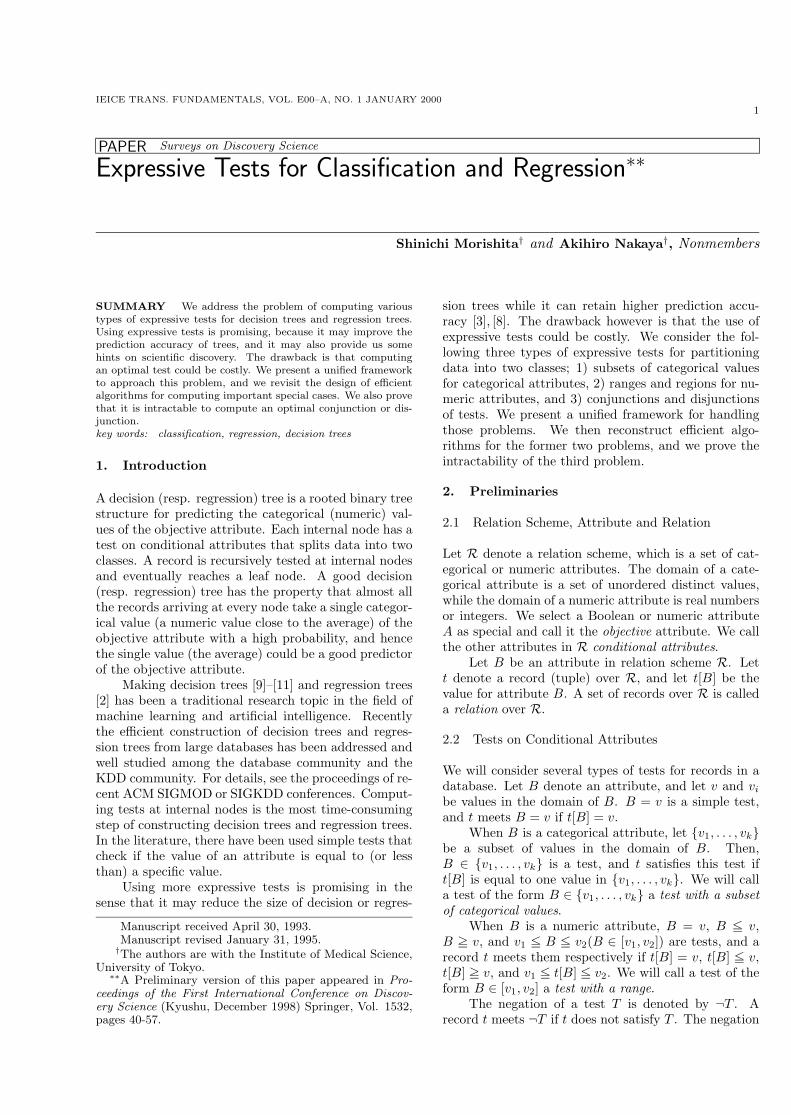
Fig. 1 (x, y), (x, y +∆), (x−∆, y), (x, y −∆), and (x +∆, y)

We first assume that lower value of φ(x, y) indi-cates higher effectiveness of the splitting. It does notmatter if we select the reverse order. The splittingby Test is most ineffective when |Rt|/|R| = m/n =|Rt

1|/|R1| = y/x = |Rt2|/|R2|, and hence φ(x, y) should

be maximum when y/x = m/n.Suppose that the probability of positive records in

R1, y/x, is greater than that of positive records in R,m/n. Also suppose that if we divide R by another newtest, the number of positive records in R1 increases by∆ (0 < ∆ <= x − y), while |R1| is the same. Then,the probability of positive records in R1, (y + ∆)/x,becomes to be greater than y/x, and hence we want toclaim that the splitting by the new test is more effec-tive. Thus we expect φ(x, y + ∆) <= φ(x, y). Similarly,since y/x <= y/(x−∆) for 0 <= ∆ < x−y we also expectφ(x−∆, y) <= φ(x, y). Figure 1 illustrates points (x, y),(x, y + ∆), and (x − ∆, y).

If the probability of positive records in R1, y/x, isless than the average m/n, then (x, y) is in the lowerside of the line connecting the origin and (m, n). SeeFigure 1. In this case observe that the probability ofpositive records in R2, which is (m − y)/(n − x), isgreater than m/n. Suppose that the number of positiverecords in R1 according to the new test decreases by ∆(0 < ∆ <= x − y), while |R1| is unchanged. Then, thenumber of positive records in R2 increases by ∆ while|R2| is the same. Thus the splitting by the new testis more effective, and we expect φ(x, y − ∆) <= φ(x, y).Similarly we also want to require φ(x+∆, y) <= φ(x, y).

In summary φ is expected to satisfy that if y/x >m/n, then φ(x, y+δ) <= φ(x, y) and φ(x−δ, y) <= φ(x, y),oherwise, φ(x, y−δ) <= φ(x, y) and φ(x+δ, y) <= φ(x, y).

Entropy of Splitting

We present an instance of φ(x, y) that meets all therequirements discussed so far. Let ent(p) = −p ln p −(1− p) ln(1− p), where p means the probability of pos-itive records in a set of records, while (1 − p) impliesthe probability of negative records. Define the entropy

MORISHITA and NAKAYA:3

Ent(x, y) of the splitting by Test as follows:

x

nent(

y

x) +

n − x

nent(

m − y

n − x),

where yx (m−y

n−x , respectively) is the probability of pos-itive records in R1 (R2). This function is known asQuinlan’s entropy heuristic [9], and it has been tradi-tionally used as a criteria for evaluating the effective-ness of the division of a set of records. Ent(x, y) isan instance of φ(x, y). We use the following theoremto show that Ent(x, y) satisfies all the requirements onφ(x, y).Theorem 2.1: Ent(x, y) is a concave function forx >= y >= 0; that is, for any (x1, y1) and (x2, y2) in{(x, y) | x >= y >= 0} and any 0 <= λ <= 1,

λEnt(x1, y1) + (1 − λ)Ent(x2, y2)<= Ent(λ(x1, y1) + (1 − λ)(x2, y2)).

Ent(x, y) is maximum when y/x = m/n.Proof: See Appendix.

We immediately obtain the following corollary.Corollary 2.1: Let (x3, y3) be an arbitrary dividingpoint of (x1, y1) and (x2, y2) in {(x, y) | x >= y >= 0};namely, (x, y) is a point on the line segment connectingthe two points. Then, min(Ent(x1, y1), Ent(x2, y2)) <=Ent(x3, y3).

For any (x, y) such that y/x > m/n and any0 < ∆ <= x − y, from the above corollary we have

min(Ent(x, y + ∆), Ent(x, (m/n)x)) <= Ent(x, y),

because (x, y) is a dividing point of (x, y + ∆) and(x, (m/n)x). Since Ent(x, (m/n)x) is maximum,

Ent(x, y + ∆) <= Ent(x, y),

and hence Ent(x, y) satisfies the requirement φ(x, y +∆) <= φ(x, y). In the same way we can show thatEnt(x, y) meets all the requirements on φ(x, y).

2.4 Splitting Criteria for Numeric Objective Attribute

Consider the case when the objective attribute A is nu-meric. Let µ(R) denote the average of A’s values in re-lation R; that is, µ(R) =

∑t∈R t[A]/|R|. Let R1 denote

again the set of records that meet a test on conditionalattributes, while let R2 denote R − R1.

In order to characterize A, it is useful to find a testsuch that µ(R1) is considerably higher than µ(R) whileµ(R2) is substantially lower than µ(R) simultaneously.To realize this criteria, we use the interclass varianceof the splitting by the test:

|R1|(µ(R1) − µ(R))2 + |R2|(µ(R2) − µ(R))2.

A test is more interesting if the interclass variance ofthe splitting by the test is larger. We also expect thatthe variance of A’s values in R1 (resp., R2) should be

small, which lets us approximate A’s values in R1 (R2)at µ(R1) (µ(R2)). To measure this property, we employthe intraclass variance of the splitting by the test:

∑t∈R1

(t[A] − µ(R1))2 +∑

t∈R2(t[A] − µ(R2))2

|R| .

We are interested in a test that maximizes the interclassvariance and also minimizes the intraclass variance atthe same time. Actually the maximization of the inter-class variance coincides with the minimization of theintraclass variance.Theorem 2.2: Given a set of tests on conditional at-tributes, the test that maximizes the interclass variancealso minimizes the intraclass variance.Proof: See Appendix.

In what follows, we will focus on the maximizationof the interclass variance. When R is given and fixed,|R|(= |R1| + |R2|) and

∑t∈R t[A] can be regarded as

constants, and let n and m denote |R| and∑

t∈R t[A]respectively. If we denote |R1| and

∑t∈R1

t[A] by x andy, the interclass variance is determined by x and y asfollows:

x(y

x− m

n)2 + (n − x)(

m − y

n − x− m

n)2,

which will be denoted by V ar(x, y). We then have thefollowing property of V ar(x, y), which is similar to The-orem 2.1 for the entropy function.Theorem 2.3: V ar(x, y) is a convex function for 0 <x < n; that is, for any (x1, y1) and (x2, y2) such thatn > x1, x2 > 0 and any 0 <= λ <= 1,

λV ar(x1, y1) + (1 − λ)V ar(x2, y2)>= V ar(λ(x1, y1) + (1 − λ)(x2, y2)).

V ar(x, y) is minimum when y/x = m/n.Proof: See Appendix.

Corollary 2.2: If (x3, y3) be an arbitrary dividingpoint of (x1, y1) and (x2, y2) such that n > x1, x2 > 0,then max(V ar(x1, y1), V ar(x2, y2)) >= V ar(x3, y3).Since the interclass variance has the property similarto the entropy function, in the following sections, wewill present how to compute the optimal test that min-imizes the entropy, but all arguments directly carry overto the case of finding the test maximizing the interclassvariance.

2.5 Positive Tests and Negative Tests

Let R be a given relation, and let R1 be the set ofrecords in R that meet a given test. If the objectiveattribute A is Boolean, we treat “true” and “false” asnumbers “1” and “0” respectively. We call the testpositive if the average of A’s values in R1 is greaterthan or equal to the average of A’s values in R; that is,(∑

t∈R1t[A])/|R1| >= (

∑t∈R t[A])/|R|. Otherwise the

4IEICE TRANS. FUNDAMENTALS, VOL. E00–A, NO. 1 JANUARY 2000

test is called negative. Thus, when A is Boolean, theprobability of positive records in R1 is greater than orequal to the probability of positive records in R.

The test that minimizes the entropy could be eitherpositive or negative. In what follows, we will focus oncomputing the positive test that minimizes the entropyof the splitting by the positive test among all the posi-tive tests. This is because the algorithm for computingthe optimal positive test can be used to calculate theoptimal negative test by exchanging “true” and “false”of the objective Boolean attribute value (or reversingthe order of the objective numeric attribute value) ineach record.

3. Computing Optimal Tests with Subsets ofCategorical Values

Let C be a conditional categorical attribute, and let{c1, c2, . . . , ck} be the domain of C. Among all thepositive tests of the form C ∈ S where S is a sub-set of {c1, c2, . . . , ck}, we want to compute the posi-tive test that minimizes the entropy of the splitting. Anaive solution would consider all the possible subsetsof {c1, c2, . . . , ck} and select the one that minimizes theentropy. Instead of investigating all 2k subsets, there isan efficient way of checking only k subsets.

We first treat “true” and “false” as real numbers“1” and “0” respectively. Assume that {t | t[C] = ci}is non-empty for simplicity. Otherwise, remove ci fromthe domain of C. For each ci, let µi denote the averageof A’s values of all the records whose C’s values are ci;that is,

µi =

∑t[C]=ci

t[A]

|{t | t[C] = ci}| .Without loss of generality we can assume that µ1 >=µ2 >= . . . >= µk, otherwise we rename the categoricalvalues appropriately to meet the above property. Wethen have the following theorem.Theorem 3.1: Among all the positive tests with sub-sets of categorical values, there exists a positive test ofthe form C ∈ {ci | 1 <= i <= j} that minimizes theentropy of the splitting.

This theorem is due to Breiman et al.[2]. Thanksto this theorem, we only need to consider k tests of theform C ∈ {ci | 1 <= i <= j} to find the optimal test. Wenow prove the theorem by using techniques introducedin the previous section.

Proof of Theorem 3.1

We will prove the case of the minimization of the en-tropy. The case of maximization of the interclass vari-ance can be shown similarly. With each subset W of{c1, c2, . . . , ck}, we associate

p(W ) = ( |{t | t[C] ∈ W}|,∑

t[C]∈W

t[A] )

in the Euclidean plane. Ent(p(W )) is the entropy ofthe splitting by the test C ∈ W . Consider the set ofall points associated with all subsets of {c1, c2, . . . , ck}.It is well known that a concave function is minimizedat the boundary of the convex hull of all those points.Since we focus on positive tests with subsets of categori-cal values, the subset W ∗ minimizing Ent(p(W ) can befound by computing the point p(W ) that maximizes

∑

t[C]∈W

t[A] − λ|{t | t[C] ∈ W}|,

where λ is a positive parameter. Consider the equality:∑

t[C]∈W

t[A] − λ|{t | t[C] ∈ W}|

=∑

ci∈W

(∑

t[C]=ci

t[A] − λ|{t | t[C] = ci}|)

=∑

ci∈W

|{t | t[C] = ci}|(µi − λ).

For the purpose of maximization, we need to excludefrom W such ci that µi−λ < 0. Thus, W ∗ = {ci | µi >=λ}. Since µ1 >= µ2 >= . . . >= µk, W ∗ = {ci | 1 <= i <= j}for some j.

4. Computing Optimal Tests with Ranges orRegions

Let B be a conditional attribute that is numeric, andlet I be a range of the domain of B. We are interestedin finding a test of the form B ∈ I that minimizes theentropy (or maximizes the interclass variance) of thesplitting by the test. When the domain of B is realnumbers, the number of candidates could be infinite.One way to cope with this problem is that we discretizethis problem by dividing the domain of B into disjointsub-ranges, say I1, . . . , IN , so that the union I1∪. . .∪IN

is the domain of B. The division of the domain, forinstance, can be done by distributing the values of Bin the given set of records into equal-sized sub-ranges.We then concatenate some successive sub-ranges, sayIi, Ii+1, . . . , Ij , to create a range Ii ∪ Ii+1 ∪ . . .∪ Ij thatoptimizes the criteria of interest.

It is natural to consider the two-dimensional ver-sion. Let B and C be numeric conditional attributes.We also simplify this problem by dividing the domainof B (resp. C) into NB (NC) equal-sized sub-ranges.We assume that NB = NC = N without loss of gen-erality as regards our algorithms. We then divide theEuclidean plane associated with B and C into N × Npixels. A grid region is a set of pixels, and let R bean instance. A record t satisfies test (B, C) ∈ R if(t[B], t[C]) belongs to R. We can consider various typesof grid regions for the purpose of splitting a relation intwo. In the literature two classes of regions have beenwell studied [3], [4], [8], [12]. An x-monotone region is

MORISHITA and NAKAYA:5

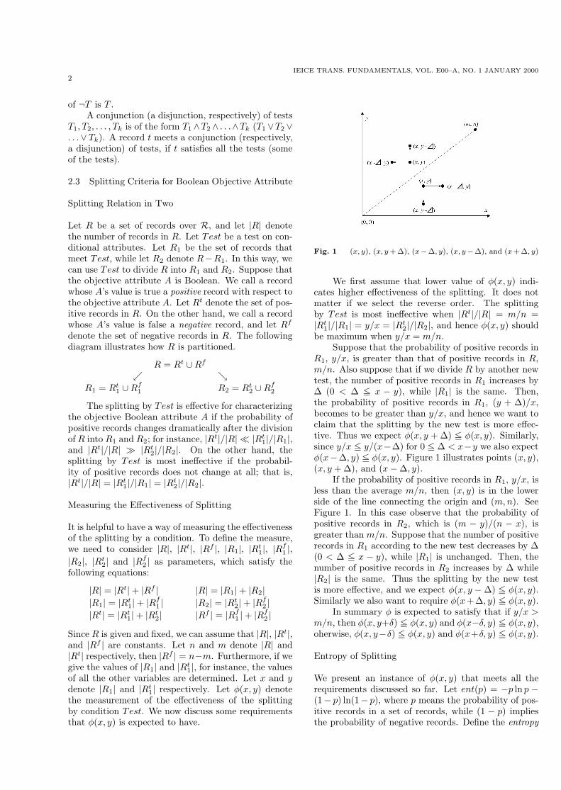
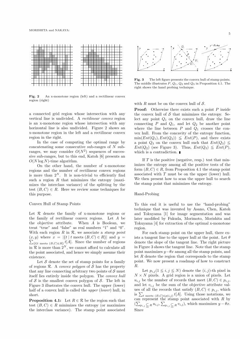
Fig. 2 An x-monotone region (left) and a rectilinear convexregion (right)

a connected grid region whose intersection with anyvertical line is undivided. A rectilinear convex regionis an x-monotone region whose intersection with anyhorizontal line is also undivided. Figure 2 shows anx-monotone region in the left and a rectilinear convexregion in the right.

In the case of computing the optimal range byconcatenating some consecutive sub-ranges of N sub-ranges, we may consider O(N2) sequences of succes-sive sub-ranges, but to this end, Katoh [6] presents anO(N log N)-time algorithm.

On the other hand, the number of x-monotoneregions and the number of rectilinear convex regionsis more than 2N . It is non-trivial to efficiently findsuch a region R that minimizes the entropy (maxi-mizes the interclass variance) of the splitting by thetest (B, C) ∈ R. Here we review some techniques forthis purpose.

Convex Hull of Stamp Points

Let R denote the family of x-monotone regions orthe family of rectilinear convex regions. Let A bethe objective attribute. When A is Boolean, wetreat “true” and “false” as real numbers “1” and “0”.With each region R in R, we associate a stamp point(x, y) where x = |{t | t meets (B, C) ∈ R}| and y =∑

{t|t meets (B,C)∈R} t[A]. Since the number of regionsin R is more than 2N , we cannot afford to calculate allthe point associated, and hence we simply assume theirexistence.

Let S denote the set of stamp points for a familyof regions R. A convex polygon of S has the propertythat any line connecting arbitrary two points of S mustitself lies entirely inside the polygon. The convex hullof S is the smallest convex polygon of S. The left inFigure 3 illustrates the convex hull. The upper (lower)half of a convex hull is called the upper (lower) hull, inshort.Proposition 4.1: Let R ∈ R be the region such thattest (B, C) ∈ R minimizes the entropy (or maximizesthe interclass variance). The stamp point associated

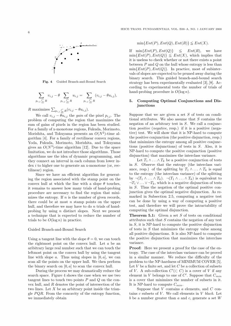
Fig. 3 The left figure presents the convex hull of stamp points.The middle illustrates P , Q1, Q2 and Q3 in Proposition 4.1. Theright shows the hand probing technique.

with R must be on the convex hull of S.Proof: Otherwise there exists such a point P insidethe convex hull of S that minimizes the entropy. Se-lect any point Q1 on the convex hull, draw the lineconnecting P and Q1, and let Q2 be another pointwhere the line between P and Q1 crosses the con-vex hull. From the concavity of the entropy function,min(Ent(Q1), Ent(Q2)) <= Ent(P ), and there existsa point Q3 on the convex hull such that Ent(Q3) <=Ent(Q2) (see Figure 3). Thus, Ent(Q3) <= Ent(P ),which is a contradiction.

If T is the positive (negative, resp.) test that min-imizes the entropy among all the positive tests of theform (B, C) ∈ R, from Proposition 4.1 the stamp pointassociated with T must be on the upper (lower) hull.We then present how to scan the upper hull to searchthe stamp point that minimizes the entropy.

Hand-Probing

To this end it is useful to use the “hand-probing”technique that was invented by Asano, Chen, Katohand Tokuyama [1] for image segmentation and waslater modified by Fukuda, Morimoto, Morishita andTokuyama [4] for extraction of the optimal x-monotoneregion.

For each stamp point on the upper hull, there ex-ists a tangent line to the upper hull at the point. Let θdenote the slope of the tangent line. The right picturein Figure 3 shows the tangent line. Note that the stamppoint maximizes y−θx among all the stamp points, andlet R denote the region that corresponds to the stamppoint. We now present a roadmap of how to constructR.

Let pi,j(1 <= i, j <= N) denote the (i, j)-th pixel inN × N pixels. A grid region is a union of pixels. Letui,j be the number of records that meet (B, C) ∈ pi,j ,and let vi,j be the sum of the objective attribute val-ues of all the records that satisfy (B, C) ∈ pi,j , whichis

∑t meets (B,C)∈p(i,j) t[A]. Using those notations, we

can represent the stamp point associated with R by(∑

pi,j ⊂=R ui,j ,∑

pi,j ⊂=R vi,j), which maximizes y − θx.

Since

6IEICE TRANS. FUNDAMENTALS, VOL. E00–A, NO. 1 JANUARY 2000

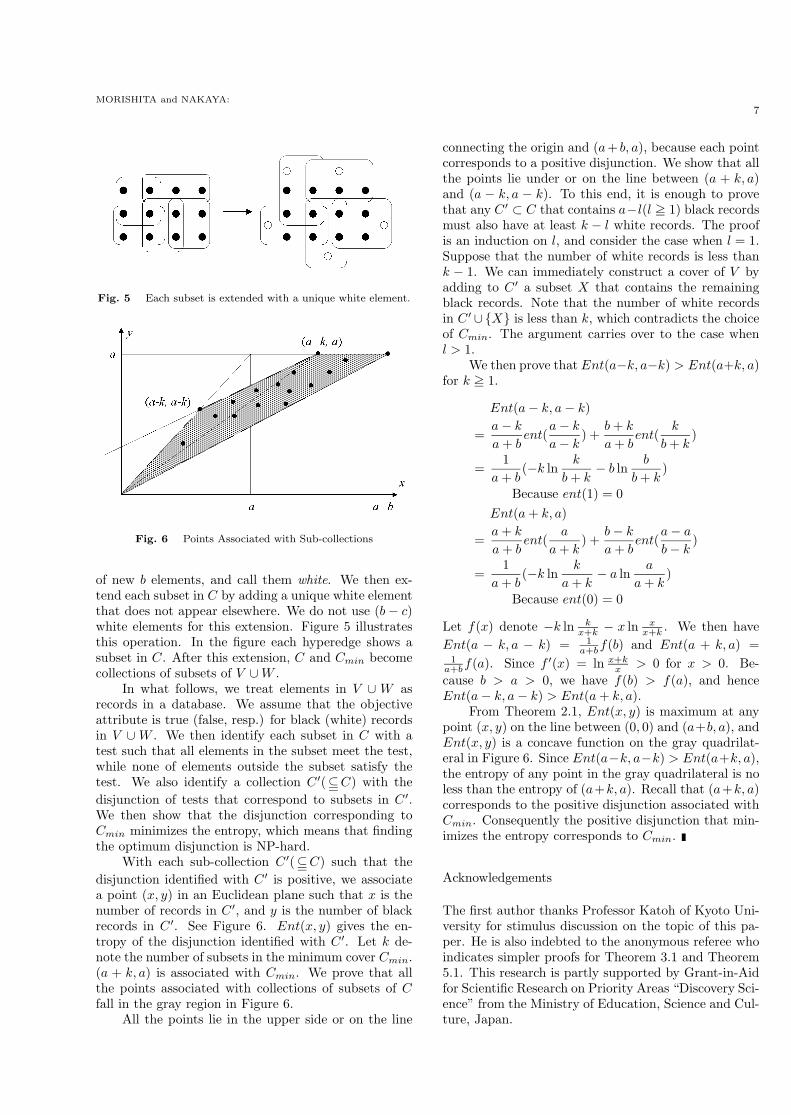
Fig. 4 Guided Branch-and-Bound Search

∑

pi,j ⊂=R

vi,j − θ∑

pi,j ⊂=R

ui,j =∑

pi,j ⊂=R

(vi,j − θui,j),

R maximizes∑

pi,j ⊂=R(vi,j − θui,j).

We call vi,j − θui,j the gain of the pixel pi,j . Theproblem of computing the region that maximizes thesum of gains of pixels in the region has been studied.For a family of x-monotone regions, Fukuda, Morimoto,Morishita, and Tokuyama presents an O(N2)-time al-gorithm [4]. For a family of rectilinear convex regions,Yoda, Fukuda, Morimoto, Morishita, and Tokuyamagives an O(N3)-time algorithm [12]. Due to the spacelimitation, we do not introduce those algorithms. Thosealgorithms use the idea of dynamic programming, andthey connect an interval in each column from lower in-dex i to higher one to generate an x-monotone (or, rec-tilinear) region.

Since we have an efficient algorithm for generat-ing the region associated with the stamp point on theconvex hull at which the line with a slope θ touches,it remains to answer how many trials of hand-probingprocedure are necessary to find the region that mini-mizes the entropy. If n is the number of given records,there could be at most n stamp points on the upperhull, and therefore we may have to do n trials of hand-probing by using n distinct slopes. Next we presenta technique that is expected to reduce the number oftrials to be O(log n) in practice.

Guided Branch-and-Bound Search

Using a tangent line with the slope θ = 0, we can touchthe rightmost point on the convex hull. Let a be anaribitrary large real number such that we can touch theleftmost point on the convex hull by using the tangentline with slope a. Thus using slopes in [0, a], we canscan all the points on the upper hull. We then performthe binary search on [0, a] to scan the convex hull.

During the process we may dramatically reduce thesearch space. Figure 4 shows the case when we use twotangent lines to touch two points P and Q on the con-vex hull, and R denotes the point of intersection of thetwo lines. Let X be an arbitrary point inside the trian-gle PQR. From the concavity of the entropy function,we immediately obtain

min{Ent(P ), Ent(Q), Ent(R)} <= Ent(X).

If min{Ent(P ), Ent(Q)} <= Ent(R), we havemin{Ent(P ), Ent(Q)} <= Ent(X), which implies thatit is useless to check whether or not there exists a pointbetween P and Q on the hull whose entropy is less thanmin{Ent(P ), Ent(Q)}. In practice, most of subinter-vals of slopes are expected to be pruned away during thebinary search. This guided branch-and-bound searchstrategy has been experimentally evaluated [3], [8]. Ac-cording to experimental tests the number of trials ofhand-probing procedure is O(log n).

5. Computing Optimal Conjunctions and Dis-junctions

Suppose that we are given a set S of tests on condi-tional attributes. We also assume that S contains thenegation of an arbitrary test in S. We call a conjunc-tion positive (negative, resp.) if it is a positive (nega-tive) test. We will show that it is NP-hard to computethe positive conjunction (the positive disjunction, resp.)that minimizes the entropy among all positive conjunc-tions (positive disjunctions) of tests in S. Also, it isNP-hard to compute the positive conjunction (positivedisjunction) that maximizes the interclass variance.

Let T1 ∧ . . .∧ Tk be a positive conjunction of testsin S. Observe that the entropy (the interclass vari-ance, resp.) of the splitting by T1 ∧ . . . ∧ Tk is equalto the entropy (the interclass variance) of the splittingby ¬(T1 ∧ . . . ∧ Tk). ¬(T1 ∧ . . . ∧ Tk) is equivalent to¬T1 ∨ . . .∨¬Tk, which is a negative disjunction of testsin S. Thus the negation of the optimal positive con-junction gives the optimal negative disjunction. As re-marked in Subsection 2.5, computing a negative testcan be done by using a way of computing a positivetest, and therefore we will prove the intractability ofcomputing the optimal disjunction.Theorem 5.1: Given a set S of tests on conditionalattributes such that S contains the negation of any testin S, it is NP-hard to compute the positive disjunctionof tests in S that minimizes the entropy value amongall positive disjunctions. It is also NP-hard to computethe positive disjunction that maximizes the interclassvariance.Proof: Here we present a proof for the case of the en-tropy. The case of the interclass variance can be provedin a similar manner. We reduce the difficulty of theproblem to the NP-hardness of MINIMUM COVER [5].Let V be a finite set, and let C be a collection of subsetsof V . A sub-collection C ′(⊂ C) is a cover of V if anyelement in V belongs to one of C ′. Suppose that Cmin

is a cover that minimizes the number of subsets in it.It is NP-hard to compute Cmin.

Suppose that V contains a elements, and C con-tains c subsets of V . We call elements in V black. Letb be a number greater than a and c, generate a set W

MORISHITA and NAKAYA:7

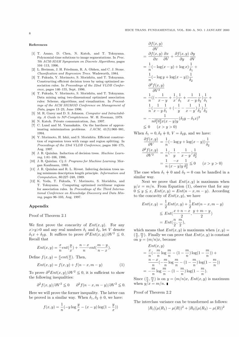
Fig. 5 Each subset is extended with a unique white element.

Fig. 6 Points Associated with Sub-collections

of new b elements, and call them white. We then ex-tend each subset in C by adding a unique white elementthat does not appear elsewhere. We do not use (b − c)white elements for this extension. Figure 5 illustratesthis operation. In the figure each hyperedge shows asubset in C. After this extension, C and Cmin becomecollections of subsets of V ∪ W .

In what follows, we treat elements in V ∪ W asrecords in a database. We assume that the objectiveattribute is true (false, resp.) for black (white) recordsin V ∪ W . We then identify each subset in C with atest such that all elements in the subset meet the test,while none of elements outside the subset satisfy thetest. We also identify a collection C ′(⊂=C) with thedisjunction of tests that correspond to subsets in C ′.We then show that the disjunction corresponding toCmin minimizes the entropy, which means that findingthe optimum disjunction is NP-hard.

With each sub-collection C ′(⊂=C) such that thedisjunction identified with C ′ is positive, we associatea point (x, y) in an Euclidean plane such that x is thenumber of records in C ′, and y is the number of blackrecords in C ′. See Figure 6. Ent(x, y) gives the en-tropy of the disjunction identified with C ′. Let k de-note the number of subsets in the minimum cover Cmin.(a + k, a) is associated with Cmin. We prove that allthe points associated with collections of subsets of Cfall in the gray region in Figure 6.

All the points lie in the upper side or on the line

connecting the origin and (a+ b, a), because each pointcorresponds to a positive disjunction. We show that allthe points lie under or on the line between (a + k, a)and (a − k, a − k). To this end, it is enough to provethat any C ′ ⊂ C that contains a−l(l >= 1) black recordsmust also have at least k − l white records. The proofis an induction on l, and consider the case when l = 1.Suppose that the number of white records is less thank − 1. We can immediately construct a cover of V byadding to C ′ a subset X that contains the remainingblack records. Note that the number of white recordsin C ′ ∪{X} is less than k, which contradicts the choiceof Cmin. The argument carries over to the case whenl > 1.

We then prove that Ent(a−k, a−k) > Ent(a+k, a)for k >= 1.

Ent(a − k, a − k)

=a − k

a + bent(

a − k

a − k) +

b + k

a + bent(

k

b + k)

=1

a + b(−k ln

k

b + k− b ln

b

b + k)

Because ent(1) = 0Ent(a + k, a)

=a + k

a + bent(

a

a + k) +

b − k

a + bent(

a − a

b − k)

=1

a + b(−k ln

k

a + k− a ln

a

a + k)

Because ent(0) = 0

Let f(x) denote −k ln kx+k − x ln x

x+k . We then haveEnt(a − k, a − k) = 1

a+bf(b) and Ent(a + k, a) =1

a+bf(a). Since f ′(x) = ln x+kx > 0 for x > 0. Be-

cause b > a > 0, we have f(b) > f(a), and henceEnt(a − k, a − k) > Ent(a + k, a).

From Theorem 2.1, Ent(x, y) is maximum at anypoint (x, y) on the line between (0, 0) and (a+b, a), andEnt(x, y) is a concave function on the gray quadrilat-eral in Figure 6. Since Ent(a−k, a−k) > Ent(a+k, a),the entropy of any point in the gray quadrilateral is noless than the entropy of (a+k, a). Recall that (a+k, a)corresponds to the positive disjunction associated withCmin. Consequently the positive disjunction that min-imizes the entropy corresponds to Cmin.

Acknowledgements

The first author thanks Professor Katoh of Kyoto Uni-versity for stimulus discussion on the topic of this pa-per. He is also indebted to the anonymous referee whoindicates simpler proofs for Theorem 3.1 and Theorem5.1. This research is partly supported by Grant-in-Aidfor Scientific Research on Priority Areas “Discovery Sci-ence” from the Ministry of Education, Science and Cul-ture, Japan.

8IEICE TRANS. FUNDAMENTALS, VOL. E00–A, NO. 1 JANUARY 2000

References

[1] T. Asano, D. Chen, N. Katoh, and T. Tokuyama.Polynomial-time solutions to image segmentations. In Proc.7th ACM-SIAM Symposium on Discrete Algorithms, pages104–113, 1996.

[2] L. Breiman, J. H. Friedman, R. A. Olshen, and C. J. Stone.Classification and Regression Trees. Wadsworth, 1984.

[3] T. Fukuda, Y. Morimoto, S. Morishita, and T. Tokuyama.Constructing efficient decision trees by using optimized as-sociation rules. In Proceedings of the 22nd VLDB Confer-ence, pages 146–155, Sept. 1996.

[4] T. Fukuda, Y. Morimoto, S. Morishita, and T. Tokuyama.Data mining using two-dimensional optimized associationrules: Scheme, algorithms, and visualization. In Proceed-ings of the ACM SIGMOD Conference on Management ofData, pages 13–23, June 1996.

[5] M. R. Garey and D. S. Johnson. Computer and Intractabil-ity. A Guide to NP-Completeness. W. H. Freeman, 1979.

[6] N. Katoh. Private communication, Jan. 1997.[7] C. Lund and M. Yannakakis. On the hardness of approx-

imating minimization problems. J.ACM, 41(5):960–981,1994.

[8] Y. Morimoto, H. Ishii, and S. Morishita. Efficient construc-tion of regression trees with range and region splitting. InProceedings of the 23rd VLDB Conference, pages 166–175,Aug. 1997.

[9] J. R. Quinlan. Induction of decision trees. Machine Learn-ing, 1:81–106, 1986.

[10] J. R. Quinlan. C4.5: Programs for Machine Learning. Mor-gan Kaufmann, 1993.

[11] J. R. Quinlan and R. L. Rivest. Inferring decision trees us-ing minimum description length principle. Information andComputation, 80:227–248, 1989.

[12] K. Yoda, T. Fukuda, Y. Morimoto, S. Morishita, andT. Tokuyama. Computing optimized rectilinear regionsfor association rules. In Proceedings of the Third Interna-tional Conference on Knowledge Discovery and Data Min-ing, pages 96–103, Aug. 1997.

Appendix

Proof of Theorem 2.1

We first prove the concavity of Ent(x, y). For anyx>y>0 and any real numbers δ1 and δ2, let V denoteδ1x + δ2y. It suffices to prove ∂2Ent(x, y)/∂V 2 <= 0.Recall that

Ent(x, y) =x

nent(

y

x) +

n − x

nent(

m − y

n − x).

Define f(x, y) = xnent( y

x ). Then,

Ent(x, y) = f(x, y) + f(n − x, m − y) (1)

To prove ∂2Ent(x, y)/∂V 2 <= 0, it is sufficient to showthe following inequalities:

∂2f(x, y)/∂V 2 <= 0 ∂2f(n − x, m − y)/∂V 2 <= 0.

Here we will prove the former inequality. The latter canbe proved in a similar way. When δ1, δ2 |= 0, we have:

f(x, y) =1n

(−y logy

x− (x − y) log(1 − y

x))

∂f(x, y)∂V

=∂f(x, y)

∂x

∂x

∂V+

∂f(x, y)∂y

∂y

∂V

=1n

(− log(x − y) + log x)1δ1

+

1n

(− log y + log(x − y))1δ2

∂2f(x, y)∂V 2

=1n

((− 1x − y

+1x

)1δ1

+1

x − y

1δ2

)1δ1

+

1n

(1

x − y

1δ1

+ (−1y− 1

x − y)

1δ2

)1δ2

= − 1nδ2

1δ22x(x − y)y

(δ2y − δ1x)2

<= 0 (x > y > 0)

When δ1 = 0, δ2 |= 0, V = δ2y, and we have:∂f(x, y)

∂V=

1n

(− log y + log(x − y))1δ2

∂2f(x, y)∂V 2

=1n

(−1y− 1

x − y)

1δ22

=1n

−x

(x − y)y1δ22

<= 0 (x > y > 0)

The case when δ1 |= 0 and δ2 = 0 can be handled in asimilar way.

Next we prove that Ent(x, y) is maximum wheny/x = m/n. From Equation (1), observe that for any0 <= y <= x, Ent(x, y) = Ent(n − x, m − y). Accordingto the concavity of Ent(x, y), we have

Ent(x, y) =12Ent(x, y) +

12Ent(n − x, m − y)

<= Ent(x + n − x

2,y + m − y

2)

= Ent(n

2,m

2),

which means that Ent(x, y) is maximum when (x, y) =(n

2 , m2 ). Finally we can prove that Ent(x, y) is constant

on y = (m/n)x, because

Ent(x, y)

=x

n(−m

nlog

m

n− (1 − m

n) log(1 − m

n)) +

n − x

n(−m

nlog

m

n− (1 − m

n) log(1 − m

n))

= −m

nlog

m

n− (1 − m

n) log(1 − m

n).

Since (n2 , m

2 ) is on y = (m/n)x, Ent(x, y) is maximumwhen y/x = m/n.

Proof of Theorem 2.2

The interclass variance can be transformed as follows:

|R1|(µ(R1) − µ(R))2 + |R2|(µ(R2) − µ(R))2

MORISHITA and NAKAYA:9

= −|R|µ(R)2 + (|R1|µ(R1)2 + |R2|µ(R2)2),

because |R| = |R1|+ |R2| and |R1|µ(R1)+ |R2|µ(R2) =|R|µ(R). Since |R| and µ(R) are constants, the maxi-mization of the interclass variance is equivalent to themaximization of |R1|µ(R1)2 + |R2|µ(R2)2.

On the other hand, the intraclass variance can betransformed as follows:

∑t∈R1

(t[A] − µ(R1))2 +∑

t∈R2(t[A] − µ(R2))2

|R|

=∑

t∈R t[A]2 − (|R1|µ(R1)2 + |R2|µ(R2)2)|R| ,

because∑

t∈R1t[A] = |R1|µ(R1) and

∑t∈R2

t[A] =|R2|µ(R2). Since R is fixed,

∑t∈R t[A]2 is a con-

stant. Thus the minimization of the intraclass vari-ance is equivalent to the maximization of |R1|µ(R1)2 +|R2|µ(R2)2 that is also equivalent to the maximizationof the interclass variance.

Proof of Theorem 2.3

The proof is similar to the proof of Theorem 2.1.We first prove that V ar(x, y) is a convex function for0 < x < n. For any 0 < x < n and any δ1 and δ2, letV denote δ1x + δ2y. Here we will prove the case whenδ1, δ2 |= 0. The other cases can be shown similarly. Itis sufficient to prove that ∂2V ar(x, y)/∂V 2 >= 0. Recallthat

V ar(x, y) = x(y

x− m

n)2 + (n − x)(

m − y

n − x− m

n)2.

Define g(x, y) = x( yx − m

n )2. Then,

V ar(x, y) = g(x, y) + g(n − x, m − y). (2)

We prove ∂2V ar(x, y)/∂V 2 >= 0 by showing the follow-ing two inequalities:

∂2g(x, y)/∂V 2 >= 0 ∂2g(n − x, m − y)/∂V 2 >= 0.

We prove the former case. The latter can be shown ina similar manner.

∂g(x, y)∂V

=∂g(x, y)

∂x

∂x

∂V+

∂g(x, y)∂y

∂y

∂V

=1δ1

{(m

n)2 − (

y

x)2} +

2δ2

(y

x− m

n)

∂2g(x, y)∂V 2

=2x

(y

δ1x− 1

δ2)2 >= 0

Next we prove that V ar(x, y) is minimum wheny/x = m/n. From Equation (2), we have V ar(x, y) =V ar(n − x, m − y). From the convexity of V ar(x, y),

V ar(x, y) =12V ar(x, y) +

12V ar(n − x, m − y)

>= V ar(x + n − x

2,y + m − y

2)

= V ar(n

2,m

2),

which implies that V ar(x, y) is minimum when (x, y) =(n

2 , m2 ). It is easy to see that V ar(x, y) = 0 when

y/x = m/n. Since (n2 , m

2 ) is on y/x = m/n, V ar(x, y)is minimum when y/x = m/n.

Shinichi Morishita Shinichi Mor-ishita is an associate professor of Depart-ment of Complexity Science and Engi-neering, Graduate School of Frontier Sci-ences, University of Tokyo. His cur-rent research interests are database queryoptimization, web-based database sys-tems, data mining and genome informat-ics. Email: moris@is.s.u-tokyo.ac.jp

Akihiro Nakaya He is a researcherat Institute of Medical Science, Universityof Tokyo, and holds BS (1994) and MS(1996) in information science from Uni-versity of Tokyo.