ship effect neutron measurements and impacts on … ship effect neutron measurements and impacts on...
TRANSCRIPT
PNNL-22953
Prepared for the U.S. Department of Energy under Contract DE-AC05-76RL01830
Ship Effect Neutron Measurements and Impacts on Low-Background Experiments Estanislao Aguayo Richard T. Kouzes Edward R. Siciliano October 2013
DISCLAIMER This report was prepared as an account of work sponsored by an agency of the United States Government. Neither the United States Government nor any agency thereof, nor Battelle Memorial Institute, nor any of their employees, makes any warranty, express or implied, or assumes any legal liability or responsibility for the accuracy, completeness, or usefulness of any information, apparatus, product, or process disclosed, or represents that its use would not infringe privately owned rights. Reference herein to any specific commercial product, process, or service by trade name, trademark, manufacturer, or otherwise does not necessarily constitute or imply its endorsement, recommendation, or favoring by the United States Government or any agency thereof, or Battelle Memorial Institute. The views and opinions of authors expressed herein do not necessarily state or reflect those of the United States Government or any agency thereof.
PACIFIC NORTHWEST NATIONAL LABORATORY operated by BATTELLE
for the UNITED STATES DEPARTMENT OF ENERGY
under Contract DE-AC05-76RL01830
Printed in the United States of America
Available to DOE and DOE contractors from the
Office of Scientific and Technical Information, P.O. Box 62, Oak Ridge, TN 37831-0062;
ph: (865) 576-8401 fax: (865) 576-5728
email: [email protected] Available to the public from the National Technical Information Service,
U.S. Department of Commerce, 5285 Port Royal Rd., Springfield, VA 22161 ph: (800) 553-6847 fax: (703) 605-6900
email: [email protected] online ordering: http://www.ntis.gov/ordering.htm
PNNL-22953
Ship Effect Neutron Measurements and Impacts on Low-Background Experiments
Estanislao Aguayo Richard T. Kouzes Edward R. Siciliano
October 2013
Pacific Northwest National Laboratory Richland, Washington 99352
Page iv of x
Abstract
The primary particles entering the upper atmosphere as cosmic rays create showers in the atmosphere that include a broad spectrum of secondary neutrons, muons and protons. These cosmic ray secondaries interact with materials at the surface of the Earth, yielding prompt backgrounds in radiation detection systems, as well as inducing long-lived activities through spallation events, dominated by the higher-energy neutron secondaries. For historical reasons, the multiple neutrons produced in spallation cascade events are referred to as “ship effect” neutrons. Quantifying the background from cosmic ray induced activities is important to low-background experiments, such as neutrinoless double-beta decay.
Since direct measurements of the effects of shielding on the cosmic ray neutron spectrum are not available, Monte Carlo modeling is used to compute such effects. However, there are large uncertainties (orders of magnitude) in the possible cross-section libraries and the cosmic ray neutron spectrum for the energy range needed in such calculations.
The measurements reported here were initiated to validate results from Monte Carlo models through experimental measurements in order to provide some confidence in the model results.
The results indicate that the models provide the correct trends of neutron production with increasing density, but there is substantial disagreement between the models and experimental results for the lower-density materials of Al, Fe and Cu.
Page v of x
Acronyms and Abbreviations
A ADC
cps DOE
ε GE
Atomic number Analog to digital converter
Counts per second U.S. Department of Energy
Detection efficiency General Electric
HDPE INC
MCNP PNNL
R+A TTL
VME
High Density Polyethylene Inter-nuclear cascade
Monte Carlo N-Particle Pacific Northwest National Laboratory
Reals plus accidentals analysis method Transistor-transistor logic
Versa Module Eurocard
Page vi of x
Contents
Abstract .......................................................................................................................................... iv
Acronyms and Abbreviations ......................................................................................................... v
Contents ......................................................................................................................................... vi
Figures and Tables ....................................................................................................................... viii
1. Introduction .............................................................................................................................. 1
1.1. Motivation for This Study ................................................................................................. 1
1.2. Cosmic Ray Neutron Spectra ............................................................................................ 2
1.3. Neutron Cross-Sections .................................................................................................... 3
1.4. Samples Used .................................................................................................................... 8
1.5. Measurements ................................................................................................................... 8
2. Multiplicity Counter System .................................................................................................. 10
3. Neutron Efficiency and Gamma Ray Sensitivity Measurements .......................................... 15
4. Muon Measurements .............................................................................................................. 16
5. Background Measurements .................................................................................................... 17
6. Polyethylene Run ................................................................................................................... 20
7. Aluminum Run ...................................................................................................................... 22
8. Steel Run ................................................................................................................................ 24
9. Copper Run ............................................................................................................................ 26
10. Lead Run .............................................................................................................................. 29
11. Tungsten Run ....................................................................................................................... 32
12. Experimental Results ........................................................................................................... 35
12.1. Integrated Experimental Multiplicity Counts ............................................................... 35
12.2. Multiplicity Rate ........................................................................................................... 36
12.3. Reals and Accidentals Multiplicity Analysis ................................................................ 38
13. Geant4 Monte Carlo Modeling ............................................................................................ 41
13.1. Geant4 Multiplicity Results .......................................................................................... 41
13.2. Geant4 Monoenergetic Neutrons .................................................................................. 43
13.3. Geant4 Total Neutron Production ................................................................................. 43
Page vii of x
13.4. Geant4 Outgoing Neutron Energy Spectra ................................................................... 45
13.5. Geant4 Incoming Cosmic Neutron Energy Spectra ...................................................... 46
14. MCNPX Monte Carlo Model Comparisons ........................................................................ 47
14.1. MCNP Monoenergetic Neutron Results ....................................................................... 47
14.2. MCNP Cosmic Ray Spectra ......................................................................................... 52
14.3. MCNP Cosmic Neutron Results ................................................................................... 54
14.4. MCNP Detection Results .............................................................................................. 56
15. Discussion of Multiplicity Results ....................................................................................... 59
16. Conclusions .......................................................................................................................... 62
17. Acknowledgements .............................................................................................................. 64
18. References ............................................................................................................................ 65
Page viii of x
Figures and Tables Figures Figure 1-1. Cutaway view of GERDA shield design ...................................................................... 1
Figure 1-2. Cosmic ray neutron energy spectra from 1 MeV to 1 GeV from various authors. ...... 3
Figure 1-3. Differential neutron cross-section example. ................................................................ 4
Figure 1-4. Total cross section for neutron processes in polyethylene used in Geant4 .................. 5
Figure 1-5. Total cross section for neutron processes in Al used in Geant4 .................................. 5
Figure 1-6. Total cross section for neutron processes in Fe used in Geant4 .................................. 6
Figure 1-7. Total cross section for neutron processes in Cu used in Geant4 .................................. 6
Figure 1-8. Total cross section for neutron processes in Pb used in Geant4 .................................. 7
Figure 1-9. Total cross section for neutron processes in W used in Geant4 ................................... 7
Figure 2-1. Experimental set-up of the multiplicity counter and electronics at the 3440 building. ............................................................................................................................................... 11
Figure 2-2. Top view of the multiplicity counter (with polyethylene sample). ............................ 11
Figure 2-3. Side and top view of the multiplicity counter in the MCNP model. .......................... 13
Figure 2-4. Energy and position efficiency profiles for 16-tube coincidence counter used. ........ 14
Figure 4-1. Cosmic ray fluctuation in a 35 year time period, from [Ziegler 1998] ...................... 16
Figure 4-2. The uWitness detector [Aguayo 2012a]. .................................................................... 16
Figure 5-1. Distribution of neutron multiplicity events caused by cosmic neutrons without a target. .................................................................................................................................... 17
Figure 5-2. Background rates recorded before and after the runs using the different materials as a target. .................................................................................................................................... 19
Figure 6-1. Multiplicity counter open showing the HDPE in position for measurement. ............ 20
Figure 6-2. Distribution of neutron multiplicity caused by cosmic neutrons in polyethylene. .... 21
Figure 7-1. Multiplicity counter open showing the aluminum in position for measurement ....... 22
Figure 7-2. Distribution of neutron multiplicity caused by cosmic neutrons in aluminum. ......... 23
Figure 8-1. Multiplicity counter open showing the iron in position for measurement. ................ 24
Figure 8-2. Distribution of neutron multiplicity caused by cosmic neutrons in steel. .................. 25
Figure 9-1. Multiplicity counter open showing the copper in position for measurement. ............ 26
Figure 9-2. Distribution of neutron multiplicity caused by cosmic neutrons in copper. .............. 27
Figure 10-1. Multiplicity counter open showing the lead in position for measurement. .............. 29
Page ix of x
Figure 10-2. Distribution of neutron multiplicity caused by cosmic neutrons in lead. ................ 30
Figure 10-3. Distribution of neutron multiplicity caused by cosmic neutrons in lead up to 50. .. 31
Figure 11-1. Multiplicity counter open showing the tungsten in position for measurement. ....... 32
Figure 11-2. Distribution of neutron multiplicity caused by cosmic neutrons in tungsten. .......... 33
Figure 11-3. Scaling of rate with target volume of Pb. ................................................................. 34
Figure 12-1. Integrated number of events versus neutron density in 10 ms gate length. ............. 35
Figure 12-2. Integrated number of events versus neutron density in 1ms gate length. ................ 35
Figure 12-3. Event rate versus neutron density for three multiplicities. ....................................... 37
Figure 12-4. Event rate versus neutron density from [Kouzes 2008]. .......................................... 38
Figure 12-5. Measured neutron multiplicities for the materials studied. ...................................... 39
Figure 12-6. Comparison of neutron triples and quads from R+A analysis for the materials studied. .................................................................................................................................. 40
Figure 13-1. Cosmic neutron simulation results for the materials studied. .................................. 42
Figure 13-2. Cosmic neutron simulation results for low-Z materials. .......................................... 42
Figure 13-3. Simulated neutrons out from a cubic foot of material as a function of neutron density. .................................................................................................................................. 44
Figure 13-4. Simulated neutrons out from a cubic foot of material as a function of neutron density. .................................................................................................................................. 45
Figure 13-5. Spectra computed with Geant4 for neutrons exiting each of the materials. ............. 46
Figure 14-1. MCNP results for total neutrons out at several energies for various materials. ....... 48
Figure 14-2. MCNP results for 1 GeV and 100 MeV monoenergetic neutrons on various materials. ............................................................................................................................... 49
Figure 14-3. MCNP results for 10 MeV and 1 MeV monoenergetic neutrons on various materials. ............................................................................................................................... 50
Figure 14-4. Simulation of collision points and cascade tracks for 1 GeV (left) and 100 MeV (right) neutron beams on Pb. ................................................................................................. 51
Figure 14-5. MCNP incident cosmic ray neutron spectra. ............................................................ 52
Figure 14-6. MCNP incident cosmic ray proton spectra. ............................................................. 53
Figure 14-7. MCNP incident cosmic ray muon spectra. ............................................................... 53
Figure 14-8. MCNP results for cosmic ray components for various materials. ........................... 55
Figure 14-9. MCNPX and Geant4 results for total neutrons out for different materials. ............. 55
Figure 14-10. Cutaway view of the MCNPX detector model: Pb (left) and Cu (right). .............. 56
Page x of x
Figure 14-11. MCNPX results versus neutron density for neutrons out and neutrons detected with the detector in place. ............................................................................................................. 57
Figure 14-12. MCNPX results versus atomic mass for neutrons out and neutrons detected with the detector in place. ............................................................................................................. 58
Figure 15-1. Comparison of simulation to measurement for counts greater than Poisson in a 1 ms window. ................................................................................................................................. 59
Figure 15-2. Comparison of R+A analysis of measurements to simulation of counts greater than Poisson in a 1 ms window. .................................................................................................... 60
Tables
Table 1.1. Sample masses and volumes used in the runs. ............................................................... 8
Table 1.2. Measurements made as part of this study. ..................................................................... 9
Table 3.1. Source run parameters from VME system (November 28, 2012) ............................... 15
Table 3.2. Source run parameters from VME system (December 10, 2012) ................................ 15
Table 5.1. Background run results (12/10/2012) .......................................................................... 18
Table 6.1. Polyethylene run results (1/14/2013) ........................................................................... 21
Table 7.1. Aluminum run results (3/1/2013) ................................................................................ 23
Table 8.1. Steel run results (1/11/2013) ........................................................................................ 25
Table 9.1. Copper run results ........................................................................................................ 28
Table 10.1. Lead run results .......................................................................................................... 30
Table 11.1. Tungsten run results (1/11/2013) ............................................................................... 33
Table 12.1. Summary of experimental multiplicity results. .......................................................... 36
Table 12.2. Comparison of multiplicity rates from a JSR14 and the VME system. ..................... 39
Table 13.1. Geant4 model results from multiplicity analysis for various materials. .................... 43
Table 13.2. Model results for total outgoing neutrons for materials for 105 incoming neutrons. . 44
Table 13.2. Ratio of outgoing neutrons for Cu/Pb for three spectra. ............................................ 46
Table 14.1. Ratio of outgoing neutrons to incoming neutrons for Pb cube. ................................. 48
Table 14.2. MCNP results percent of unscattered incident neutrons. ........................................... 51
Table 14.3. MCNP results for total neutrons out for cosmic ray components on materials. ........ 54
Table 14.4. MCNP results for total neutrons out for cosmic ray components on materials. ........ 56
Table 15.1. Data for various materials shown in Figure 15-1. ..................................................... 59
Page 1
1. Introduction
Cosmic ray primaries create showers in the atmosphere that include a broad spectrum of neutrons, protons and muons. At the Earth’s surface, the muon flux (168 m-2s-1 [Greisen 1942]) and neutron flux (134 m-2s-1 [Gordon 2004]) are comparable, while the proton flux (2 m-2s-1 [Diggory 1974; Grieder 2001; Nakamura 2012]) is a few percent of these. These neutrons, muons and protons interact with materials at the surface of the Earth, yielding prompt backgrounds in radiation detection systems, as well as inducing long-lived activation products through spallation events. Spallation events involve a cascade of neutron interactions in a block of material following knock-out interaction that “breaks” a nucleus apart. Muon and proton induced spallation are about an order of magnitude smaller than neutron induced events at the surface of the Earth. The multiple neutrons produced in spallation events are referred to as “ship effect” neutrons.1 Quantifying the background from cosmic ray induced activities is important to low-background experiments, such as neutrinoless double-beta decay (0νββ) [Aalseth 2009].
1.1. Motivation for This Study
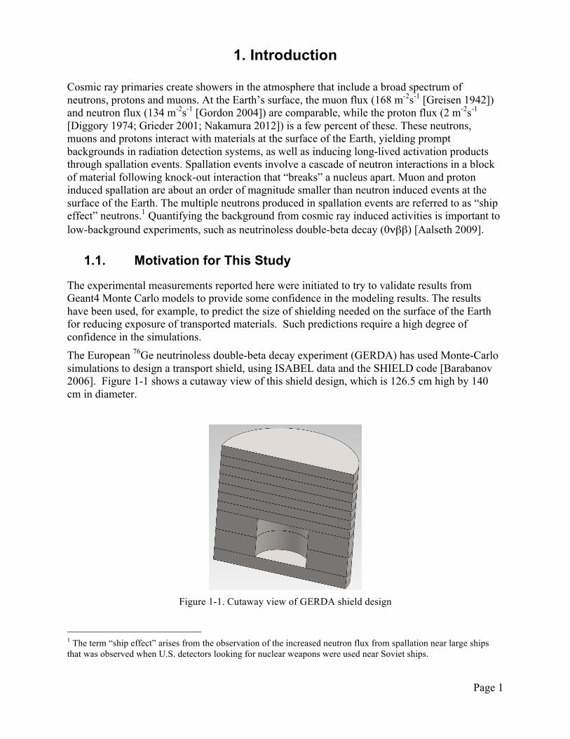
The experimental measurements reported here were initiated to try to validate results from Geant4 Monte Carlo models to provide some confidence in the modeling results. The results have been used, for example, to predict the size of shielding needed on the surface of the Earth for reducing exposure of transported materials. Such predictions require a high degree of confidence in the simulations. The European 76Ge neutrinoless double-beta decay experiment (GERDA) has used Monte-Carlo simulations to design a transport shield, using ISABEL data and the SHIELD code [Barabanov 2006]. Figure 1-1 shows a cutaway view of this shield design, which is 126.5 cm high by 140 cm in diameter.
Figure 1-1. Cutaway view of GERDA shield design
1 The term “ship effect” arises from the observation of the increased neutron flux from spallation near large ships that was observed when U.S. detectors looking for nuclear weapons were used near Soviet ships.
Page 2
The SHIELD result predicts an attenuation length for neutrons at 100 MeV in iron of about 240 g/cm2 (0.30 m). Barabanov et al. predict that the shield design of Figure 1-1 will reduce production of 68Ge and 60Co by 10 and 15, respectively. They also state that calculations using the library of excitation functions, ISABEL, gave results that were a factor of 2 to 6 lower (i.e., less production of 68Ge and 60Co due to more attenuation of neutrons predicted by ISABEL) than those obtained with their simulation tool, SHIELD.
The Geant4 model results performed for the MAJORANA DEMONSTRATOR for this same transport shield disagreed with the Barabanov simulations using SHIELD by a factor of ~2.5 for the effect of iron as a shield material [Aguayo 2012b]. Geant4 predicted a greater degree of shielding by the iron shipping shield than the SHIELD code. This difference is what motivated the current study to see how well a model could predict experimental results.
When energetic neutrons interact with nuclei in a material, they can cause spallation of the nucleus, releasing a large number of neutrons that then cascade through the material. A high efficiency thermal-neutron detector surrounding a block of material can detect some fraction of these spallation neutrons. The number of neutrons detected in a specified time window is referred to here as the “multiplicity.” Recording the timing of each detected neutron can be used to generate a histogram of the measured multiplicity. For long enough time scales, much greater than the ~0.1 millisecond thermalization time for neutrons from a spallation event, the distribution will look random (Poisson). For short time scales comparable to the neutron thermalization time (less than ~1 millisecond), high multiplicity events from the ship effect will show up in the multiplicity as a non-Poison distribution. One measure of this non-Poisson behavior is to count the number of events that exceed some multiplicity value (e.g., four or more), and such measures are used here to show the dependence of multiplicity on material type. It has been demonstrated previously that there is a strong dependence of multiplicity on material atomic mass; the current work provides a more controlled measurement than was previously reported [Kouzes 2008]. This paper reports on neutron multiplicity measurements from cosmic neutron interactions in different materials for the purpose of comparing them to predictions from Monte Carlo models. Neutron multiplicity was measured, and modeled, for commonly used shielding materials (polyethylene, aluminum, steel, copper, lead and tungsten), and the results are compared.
1.2. Cosmic Ray Neutron Spectra
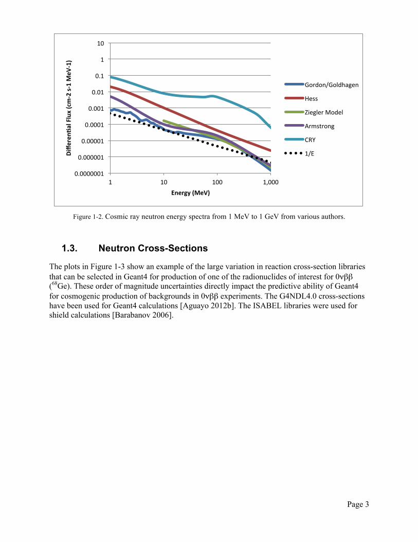
Since direct measurements of the effects of shielding on the cosmic ray neutron spectrum are not available, Monte Carlo modeling with Geant4 [Agostinelli 2003] has been used to compute such effects. However, there are large uncertainties (orders of magnitude) in the cosmic ray neutron spectrum and the possible cross-section libraries used for such calculations. Figure 1-2 shows cosmic ray neutron energy spectra from 1 MeV to 1 GeV as measured by various authors [Armstrong 1973; Gordon 2004; Hess 1959; Ziegler 1998] and computed by the CRY model [Hagmann 2008]. The energy region from about 20 MeV to 200 MeV is of most interest to production of backgrounds in materials used for 0νββ. The cosmic spectrum approximately follows an E-1 dependence, as shown by the dotted line. The CRY code results do not appear to be consistent with the experimental values for these low energies of interest. The CRY results are not used because of this discrepancy.
Page 3
Figure 1-2. Cosmic ray neutron energy spectra from 1 MeV to 1 GeV from various authors.
1.3. Neutron Cross-Sections
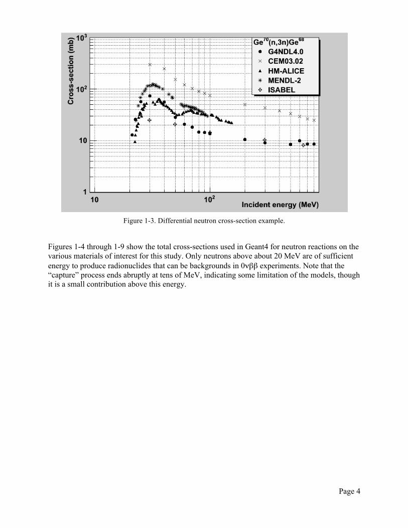
The plots in Figure 1-3 show an example of the large variation in reaction cross-section libraries that can be selected in Geant4 for production of one of the radionuclides of interest for 0νββ (68Ge). These order of magnitude uncertainties directly impact the predictive ability of Geant4 for cosmogenic production of backgrounds in 0νββ experiments. The G4NDL4.0 cross-sections have been used for Geant4 calculations [Aguayo 2012b]. The ISABEL libraries were used for shield calculations [Barabanov 2006].
0.0000001
0.000001
0.00001
0.0001
0.001
0.01
0.1
1
10
1 10 100 1,000
Diffe
ren'
al Flux (cm-‐2 s-‐1 MeV
-‐1)
Energy (MeV)
Gordon/Goldhagen
Hess
Ziegler Model
Armstrong
CRY
1/E
Page 4
Figure 1-3. Differential neutron cross-section example.
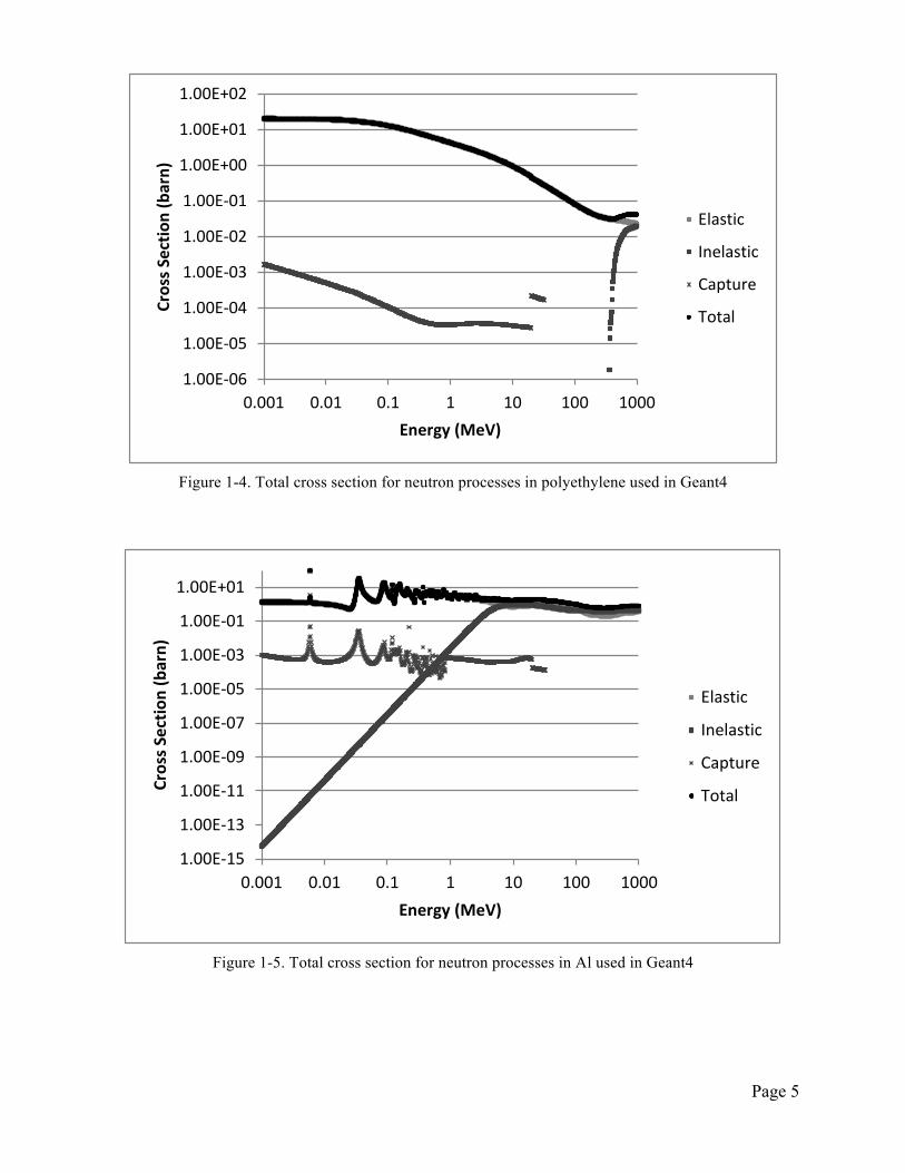
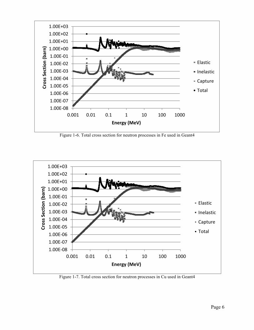
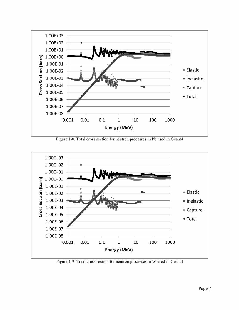
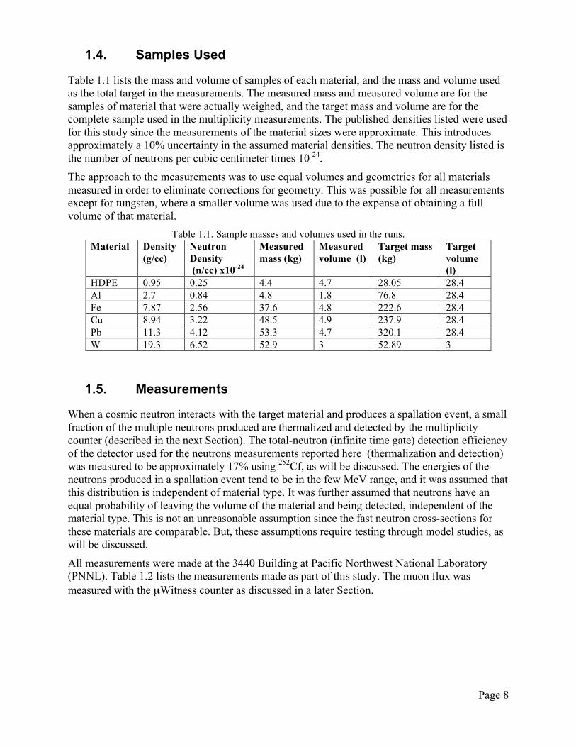
Figures 1-4 through 1-9 show the total cross-sections used in Geant4 for neutron reactions on the various materials of interest for this study. Only neutrons above about 20 MeV are of sufficient energy to produce radionuclides that can be backgrounds in 0νββ experiments. Note that the “capture” process ends abruptly at tens of MeV, indicating some limitation of the models, though it is a small contribution above this energy.
Page 5
Figure 1-4. Total cross section for neutron processes in polyethylene used in Geant4
Figure 1-5. Total cross section for neutron processes in Al used in Geant4
1.00E-‐06
1.00E-‐05
1.00E-‐04
1.00E-‐03
1.00E-‐02
1.00E-‐01
1.00E+00
1.00E+01
1.00E+02
0.001 0.01 0.1 1 10 100 1000
Cross S
ectio
n (barn)
Energy (MeV)
Elastic
Inelastic
Capture
Total
1.00E-‐15
1.00E-‐13
1.00E-‐11
1.00E-‐09
1.00E-‐07
1.00E-‐05
1.00E-‐03
1.00E-‐01
1.00E+01
0.001 0.01 0.1 1 10 100 1000
Cross S
ectio
n (barn)
Energy (MeV)
Elastic
Inelastic
Capture
Total
Page 6
Figure 1-6. Total cross section for neutron processes in Fe used in Geant4
Figure 1-7. Total cross section for neutron processes in Cu used in Geant4
1.00E-‐081.00E-‐071.00E-‐061.00E-‐051.00E-‐041.00E-‐031.00E-‐021.00E-‐011.00E+001.00E+011.00E+021.00E+03
0.001 0.01 0.1 1 10 100 1000
Cross S
ectio
n (barn)
Energy (MeV)
Elastic
Inelastic
Capture
Total
1.00E-‐081.00E-‐071.00E-‐061.00E-‐051.00E-‐041.00E-‐031.00E-‐021.00E-‐011.00E+001.00E+011.00E+021.00E+03
0.001 0.01 0.1 1 10 100 1000
Cross S
ectio
n (barn)
Energy (MeV)
Elastic
Inelastic
Capture
Total
Page 7
Figure 1-8. Total cross section for neutron processes in Pb used in Geant4
Figure 1-9. Total cross section for neutron processes in W used in Geant4
1.00E-‐081.00E-‐071.00E-‐061.00E-‐051.00E-‐041.00E-‐031.00E-‐021.00E-‐011.00E+001.00E+011.00E+021.00E+03
0.001 0.01 0.1 1 10 100 1000
Cross S
ectio
n (barn)
Energy (MeV)
Elastic
Inelastic
Capture
Total
1.00E-‐081.00E-‐071.00E-‐061.00E-‐051.00E-‐041.00E-‐031.00E-‐021.00E-‐011.00E+001.00E+011.00E+021.00E+03
0.001 0.01 0.1 1 10 100 1000
Cross S
ectio
n (barn)
Energy (MeV)
Elastic
Inelastic
Capture
Total
Page 8
1.4. Samples Used
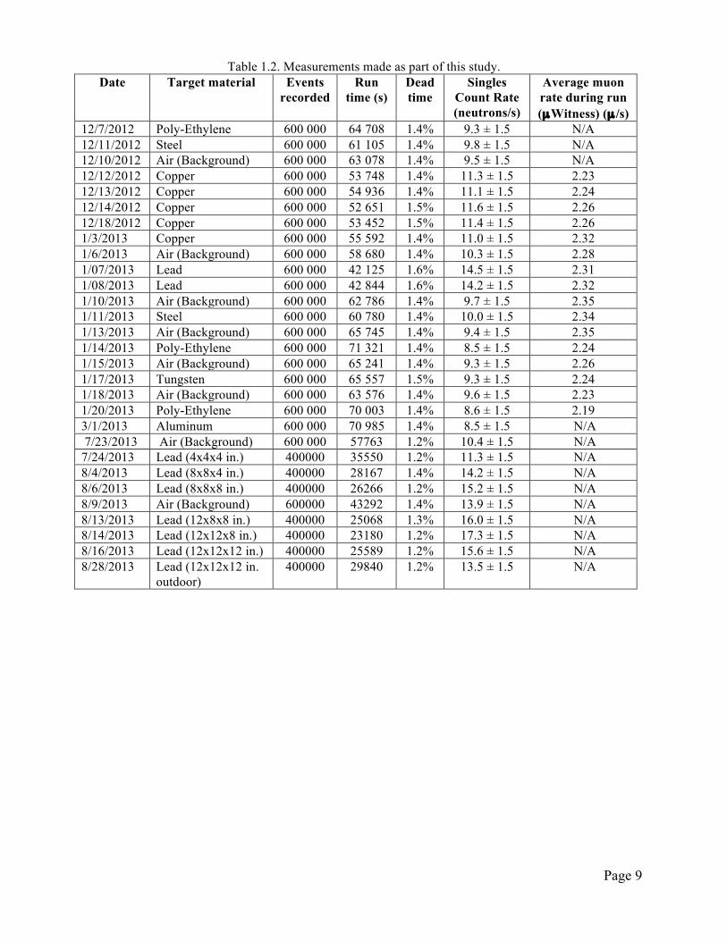
Table 1.1 lists the mass and volume of samples of each material, and the mass and volume used as the total target in the measurements. The measured mass and measured volume are for the samples of material that were actually weighed, and the target mass and volume are for the complete sample used in the multiplicity measurements. The published densities listed were used for this study since the measurements of the material sizes were approximate. This introduces approximately a 10% uncertainty in the assumed material densities. The neutron density listed is the number of neutrons per cubic centimeter times 10-24. The approach to the measurements was to use equal volumes and geometries for all materials measured in order to eliminate corrections for geometry. This was possible for all measurements except for tungsten, where a smaller volume was used due to the expense of obtaining a full volume of that material.
Table 1.1. Sample masses and volumes used in the runs. Material Density
(g/cc) Neutron Density (n/cc) x10-24
Measured mass (kg)
Measured volume (l)
Target mass (kg)
Target volume (l)
HDPE 0.95 0.25 4.4 4.7 28.05 28.4 Al 2.7 0.84 4.8 1.8 76.8 28.4 Fe 7.87 2.56 37.6 4.8 222.6 28.4 Cu 8.94 3.22 48.5 4.9 237.9 28.4 Pb 11.3 4.12 53.3 4.7 320.1 28.4 W 19.3 6.52 52.9 3 52.89 3
1.5. Measurements
When a cosmic neutron interacts with the target material and produces a spallation event, a small fraction of the multiple neutrons produced are thermalized and detected by the multiplicity counter (described in the next Section). The total-neutron (infinite time gate) detection efficiency of the detector used for the neutrons measurements reported here (thermalization and detection) was measured to be approximately 17% using 252Cf, as will be discussed. The energies of the neutrons produced in a spallation event tend to be in the few MeV range, and it was assumed that this distribution is independent of material type. It was further assumed that neutrons have an equal probability of leaving the volume of the material and being detected, independent of the material type. This is not an unreasonable assumption since the fast neutron cross-sections for these materials are comparable. But, these assumptions require testing through model studies, as will be discussed.
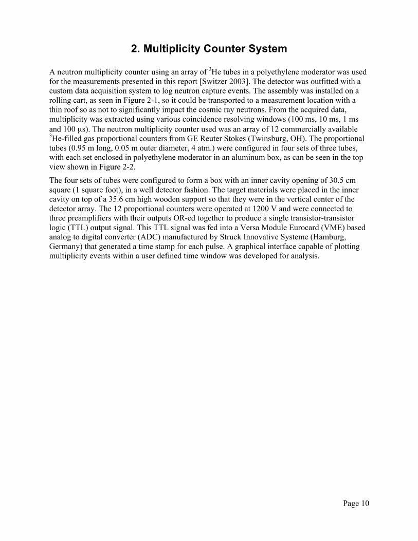
All measurements were made at the 3440 Building at Pacific Northwest National Laboratory (PNNL). Table 1.2 lists the measurements made as part of this study. The muon flux was measured with the µWitness counter as discussed in a later Section.
Page 9
Table 1.2. Measurements made as part of this study. Date Target material Events
recorded Run
time (s) Dead time
Singles Count Rate (neutrons/s)
Average muon rate during run (µWitness) (µ /s)
12/7/2012 Poly-Ethylene 600 000 64 708 1.4% 9.3 ± 1.5 N/A 12/11/2012 Steel 600 000 61 105 1.4% 9.8 ± 1.5 N/A 12/10/2012 Air (Background) 600 000 63 078 1.4% 9.5 ± 1.5 N/A 12/12/2012 Copper 600 000 53 748 1.4% 11.3 ± 1.5 2.23 12/13/2012 Copper 600 000 54 936 1.4% 11.1 ± 1.5 2.24 12/14/2012 Copper 600 000 52 651 1.5% 11.6 ± 1.5 2.26 12/18/2012 Copper 600 000 53 452 1.5% 11.4 ± 1.5 2.26 1/3/2013 Copper 600 000 55 592 1.4% 11.0 ± 1.5 2.32 1/6/2013 Air (Background) 600 000 58 680 1.4% 10.3 ± 1.5 2.28 1/07/2013 Lead 600 000 42 125 1.6% 14.5 ± 1.5 2.31 1/08/2013 Lead 600 000 42 844 1.6% 14.2 ± 1.5 2.32 1/10/2013 Air (Background) 600 000 62 786 1.4% 9.7 ± 1.5 2.35 1/11/2013 Steel 600 000 60 780 1.4% 10.0 ± 1.5 2.34 1/13/2013 Air (Background) 600 000 65 745 1.4% 9.4 ± 1.5 2.35 1/14/2013 Poly-Ethylene 600 000 71 321 1.4% 8.5 ± 1.5 2.24 1/15/2013 Air (Background) 600 000 65 241 1.4% 9.3 ± 1.5 2.26 1/17/2013 Tungsten 600 000 65 557 1.5% 9.3 ± 1.5 2.24 1/18/2013 Air (Background) 600 000 63 576 1.4% 9.6 ± 1.5 2.23 1/20/2013 Poly-Ethylene 600 000 70 003 1.4% 8.6 ± 1.5 2.19 3/1/2013 Aluminum 600 000 70 985 1.4% 8.5 ± 1.5 N/A 7/23/2013 Air (Background) 600 000 57763 1.2% 10.4 ± 1.5 N/A 7/24/2013 Lead (4x4x4 in.) 400000 35550 1.2% 11.3 ± 1.5 N/A 8/4/2013 Lead (8x8x4 in.) 400000 28167 1.4% 14.2 ± 1.5 N/A 8/6/2013 Lead (8x8x8 in.) 400000 26266 1.2% 15.2 ± 1.5 N/A 8/9/2013 Air (Background) 600000 43292 1.4% 13.9 ± 1.5 N/A 8/13/2013 Lead (12x8x8 in.) 400000 25068 1.3% 16.0 ± 1.5 N/A 8/14/2013 Lead (12x12x8 in.) 400000 23180 1.2% 17.3 ± 1.5 N/A 8/16/2013 Lead (12x12x12 in.) 400000 25589 1.2% 15.6 ± 1.5 N/A 8/28/2013 Lead (12x12x12 in.
outdoor) 400000 29840 1.2% 13.5 ± 1.5 N/A
Page 10
2. Multiplicity Counter System
A neutron multiplicity counter using an array of 3He tubes in a polyethylene moderator was used for the measurements presented in this report [Switzer 2003]. The detector was outfitted with a custom data acquisition system to log neutron capture events. The assembly was installed on a rolling cart, as seen in Figure 2-1, so it could be transported to a measurement location with a thin roof so as not to significantly impact the cosmic ray neutrons. From the acquired data, multiplicity was extracted using various coincidence resolving windows (100 ms, 10 ms, 1 ms and 100 µs). The neutron multiplicity counter used was an array of 12 commercially available 3He-filled gas proportional counters from GE Reuter Stokes (Twinsburg, OH). The proportional tubes (0.95 m long, 0.05 m outer diameter, 4 atm.) were configured in four sets of three tubes, with each set enclosed in polyethylene moderator in an aluminum box, as can be seen in the top view shown in Figure 2-2. The four sets of tubes were configured to form a box with an inner cavity opening of 30.5 cm square (1 square foot), in a well detector fashion. The target materials were placed in the inner cavity on top of a 35.6 cm high wooden support so that they were in the vertical center of the detector array. The 12 proportional counters were operated at 1200 V and were connected to three preamplifiers with their outputs OR-ed together to produce a single transistor-transistor logic (TTL) output signal. This TTL signal was fed into a Versa Module Eurocard (VME) based analog to digital converter (ADC) manufactured by Struck Innovative Systeme (Hamburg, Germany) that generated a time stamp for each pulse. A graphical interface capable of plotting multiplicity events within a user defined time window was developed for analysis.
Page 11
Figure 2-1. Experimental set-up of the multiplicity counter and electronics at the 3440 building.
Figure 2-2. Top view of the multiplicity counter (with polyethylene sample).
Page 12
The fast ADC allowed collecting multiplicity distribution information in a range from one to 80 counts in the gate width. The system was designed to minimize electronic dead time between counts using a small but fast access memory where the data is logged for up to 80 consecutive counts, then the content of this first memory is transferred to the personal computer (PC). The dead time for a memory access in the first data tier is 150 ns, whereas the dead time for the Tier 1 memory transfer to the PC is 10 ms. Having these set dead times for memory access allows for a simple calculation to determine the effective dead time of the system. The digitization frequency of this ADC is 100 MHz, with a time stamp option for every digitized pulse. This feature was used to give the system the ability to count multiplicities in a user defined gate width with multiplicity up to 80. Since the event rate was of order 10 Hz, dead time for the measurements was minimal.
The operation of the multiplicity counter was in two steps. The first step was to log every incoming pulse, along with the time stamp, into a memory buffer. The memory buffer fills up with the pre-programmed number of events to be recoded. The multiplicity counter was programmed to log a fixed number of total counts, rather than a set run time.
The second step was to apply offline analysis to this data to extract the multiplicity distribution based on the time stamps of the recorded pulses. The multiplicity distribution can be determined by generating a histogram of the number of events with a given number of pulses following in a fixed time window. In order to measure multiplicity, the algorithm looked in a time window starting with the first pulse and counted the number of pulses. For example, assume a pulse comes in at 10 µs after the counter starts operating. The next pulses come in at times 10.2 µs and 12 µs, and no pulses after a 2 µs window. If the programmed gate length was larger than 0.2 µs and smaller than 2 µs, multiplicity bin 2 would be incremented by one unit, and the multiplicity bin 1 would also be incremented by one unit. If the programmed gate width were larger than 2 µs, the multiplicity bin 3 would be incremented by one. If the gate width were shorter than 0.2 us, multiplicity bin 1 would be incremented three times. This analysis algorithm prevents double counting of pulses in different multiplicity bins. This rationale is valid for multiplicity counting in a scenario where the incoming pulse rate is below that of the inverse of the gate length time. This is required in order to be able to ignore situations were the pulse train might induce miscounting due to event pileup from different primary nuclear reactions. This is the case for cosmogenic neutron counting, where a simplistic analysis was possible since the event rate was low, making the traditional coincidence analysis of reals and accidentals unnecessary. Post analysis of the data involved determining multiplicity with time windows of 100 ms, 10 ms, 1 ms and 100 µs. Typical die-away times for coincidence counters are in the 50-100 µs regime, so a 100 µs time window is perhaps appropriate, while 100 ms window is too long, allowing the multiplicity distribution to be averaged out. Since the flux of cosmic neutrons is about 134 m-2s-1 [Gordon 2004], the average time between spallation events should be fewer than about one every 80 ms since not every neutron will produce a spallation. A 1 ms time window is reasonable for data analysis, long enough to capture the full multiplicity of events but short enough not to be contaminated by overlapping events.
An MCNP model [MCNP] of the multiplicity counter had previously been developed [Switzer 2003]. Side and top views of the model developed in that study are shown in Figure 2-3.
Page 13
Figure 2-3. Side and top view of the multiplicity counter in the MCNP model.
The MCNP model predicts an efficiency of 19.9% for a centered 252Cf source, and a die-away time of 46 µs. Thus, a time window of 60-100 µs is reasonable for counting coincidences from spallation events (which occur on a much shorter time scale). Energy and (vertical) position efficiency profiles were also calculated, as shown in Figure 2-4. The energy profile shows a reasonably flat behavior for spallation neutrons with energies between ~ 100 eV to 100 keV, a gradual fall off below 100 eV, but a rapid fall off above 100 keV. The position profile shows there can be ~10% reduction in efficiency if neutrons are emitted from the spallation block at positions ~20 cm above or below the center of the detector. These effects are automatically taken into account for MCNP calculations for finite blocks of material.
Page 14
Figure 2-4. Energy and position efficiency profiles for 16-tube coincidence counter used.
10%
15%
20%
25%
30%
1.E-‐08 1.E-‐07 1.E-‐06 1.E-‐05 1.E-‐04 1.E-‐03 1.E-‐02 1.E-‐01 1.E+00 1.E+01
Coun
t Efficien
cy
Energy (MeV)
Trial2L_new: ε vs. Neutron Energy
10%
15%
20%
25%
30%
0 10 20 30 40 50 60 70 80 90 100
Coun
t Efficien
cy
Source Position (cm)
Trial2L_new: ε vs. Source Height (above PolyBox Bottom)
Cf-‐252
Page 15
3. Neutron Efficiency and Gamma Ray Sensitivity Measurements
A gamma ray source was used to verify that the multiplicity detector threshold was adjusted appropriately to be insensitive to gamma rays. This was done by placing 137Cs (7.7 µCi) and 60Co (2.7 µCi) sources in the center of the detector and finding that there was no change in the neutron background count rate observed by the detector system.
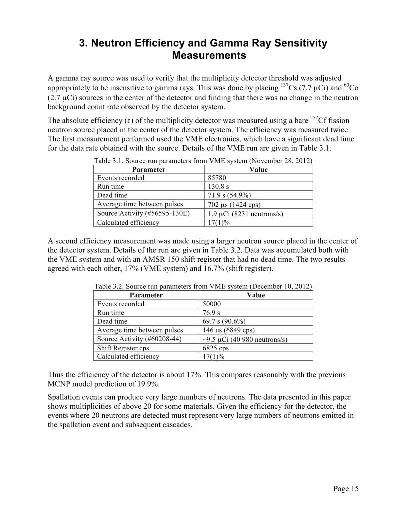
The absolute efficiency (ε) of the multiplicity detector was measured using a bare 252Cf fission neutron source placed in the center of the detector system. The efficiency was measured twice. The first measurement performed used the VME electronics, which have a significant dead time for the data rate obtained with the source. Details of the VME run are given in Table 3.1.
Table 3.1. Source run parameters from VME system (November 28, 2012) Parameter Value
Events recorded 85780 Run time 130.8 s Dead time 71.9 s (54.9%) Average time between pulses 702 µs (1424 cps) Source Activity (#56595-130E) 1.9 µCi (8231 neutrons/s) Calculated efficiency 17(1)%
A second efficiency measurement was made using a larger neutron source placed in the center of the detector system. Details of the run are given in Table 3.2. Data was accumulated both with the VME system and with an AMSR 150 shift register that had no dead time. The two results agreed with each other, 17% (VME system) and 16.7% (shift register).
Table 3.2. Source run parameters from VME system (December 10, 2012) Parameter Value
Events recorded 50000 Run time 76.9 s Dead time 69.7 s (90.6%) Average time between pulses 146 us (6849 cps) Source Activity (#60208-44) ~9.5 µCi (40 980 neutrons/s) Shift Register cps 6825 cps Calculated efficiency 17(1)%
Thus the efficiency of the detector is about 17%. This compares reasonably with the previous MCNP model prediction of 19.9%. Spallation events can produce very large numbers of neutrons. The data presented in this paper shows multiplicities of above 20 for some materials. Given the efficiency for the detector, the events where 20 neutrons are detected must represent very large numbers of neutrons emitted in the spallation event and subsequent cascades.
Page 16
4. Muon Measurements
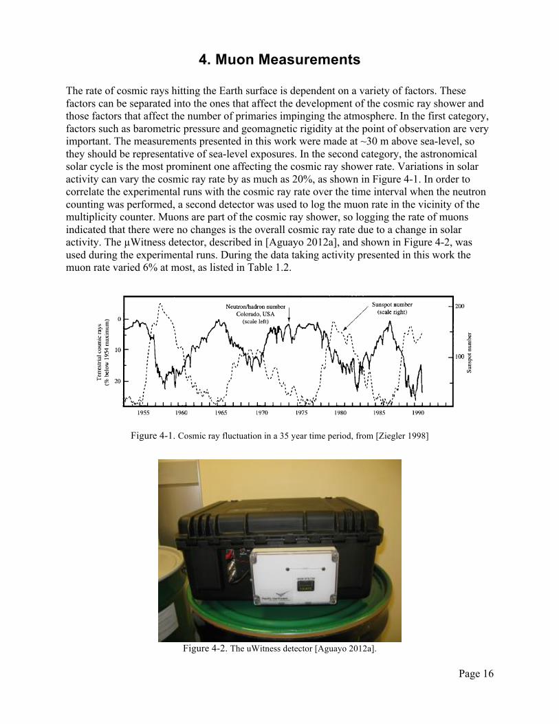
The rate of cosmic rays hitting the Earth surface is dependent on a variety of factors. These factors can be separated into the ones that affect the development of the cosmic ray shower and those factors that affect the number of primaries impinging the atmosphere. In the first category, factors such as barometric pressure and geomagnetic rigidity at the point of observation are very important. The measurements presented in this work were made at ~30 m above sea-level, so they should be representative of sea-level exposures. In the second category, the astronomical solar cycle is the most prominent one affecting the cosmic ray shower rate. Variations in solar activity can vary the cosmic ray rate by as much as 20%, as shown in Figure 4-1. In order to correlate the experimental runs with the cosmic ray rate over the time interval when the neutron counting was performed, a second detector was used to log the muon rate in the vicinity of the multiplicity counter. Muons are part of the cosmic ray shower, so logging the rate of muons indicated that there were no changes is the overall cosmic ray rate due to a change in solar activity. The µWitness detector, described in [Aguayo 2012a], and shown in Figure 4-2, was used during the experimental runs. During the data taking activity presented in this work the muon rate varied 6% at most, as listed in Table 1.2.
Figure 4-1. Cosmic ray fluctuation in a 35 year time period, from [Ziegler 1998]
Figure 4-2. The uWitness detector [Aguayo 2012a].
Page 17
5. Background Measurements
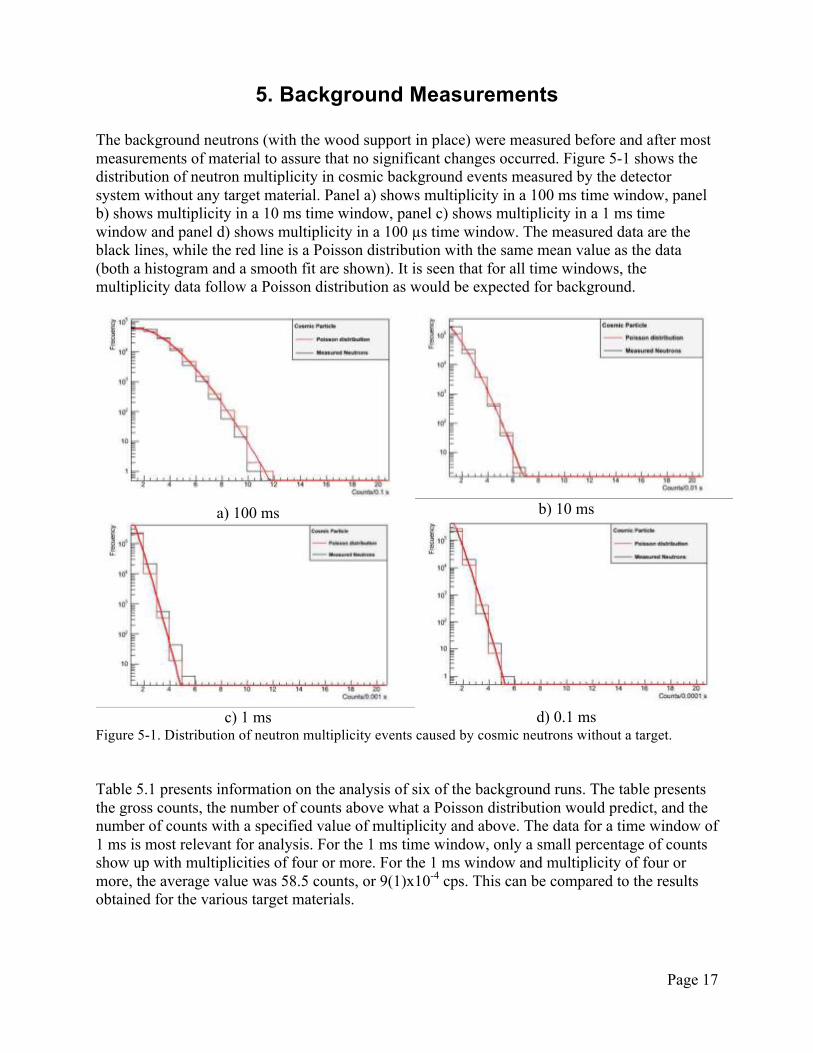
The background neutrons (with the wood support in place) were measured before and after most measurements of material to assure that no significant changes occurred. Figure 5-1 shows the distribution of neutron multiplicity in cosmic background events measured by the detector system without any target material. Panel a) shows multiplicity in a 100 ms time window, panel b) shows multiplicity in a 10 ms time window, panel c) shows multiplicity in a 1 ms time window and panel d) shows multiplicity in a 100 µs time window. The measured data are the black lines, while the red line is a Poisson distribution with the same mean value as the data (both a histogram and a smooth fit are shown). It is seen that for all time windows, the multiplicity data follow a Poisson distribution as would be expected for background.
a) 100 ms
b) 10 ms
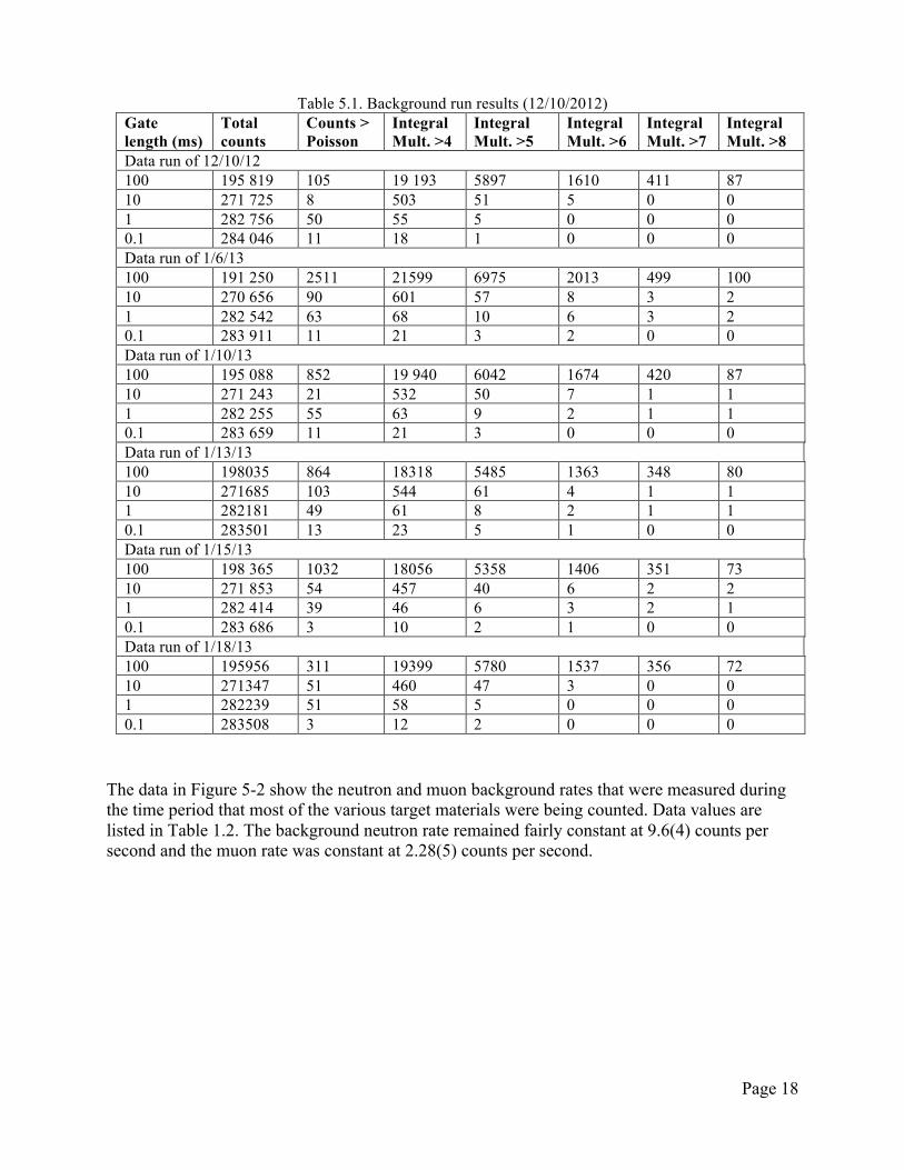
c) 1 ms d) 0.1 ms Figure 5-1. Distribution of neutron multiplicity events caused by cosmic neutrons without a target. Table 5.1 presents information on the analysis of six of the background runs. The table presents the gross counts, the number of counts above what a Poisson distribution would predict, and the number of counts with a specified value of multiplicity and above. The data for a time window of 1 ms is most relevant for analysis. For the 1 ms time window, only a small percentage of counts show up with multiplicities of four or more. For the 1 ms window and multiplicity of four or more, the average value was 58.5 counts, or 9(1)x10-4 cps. This can be compared to the results obtained for the various target materials.
Page 18
Table 5.1. Background run results (12/10/2012)
Gate length (ms)
Total counts
Counts > Poisson
Integral Mult. >4
Integral Mult. >5
Integral Mult. >6
Integral Mult. >7
Integral Mult. >8
Data run of 12/10/12 100 195 819 105 19 193 5897 1610 411 87 10 271 725 8 503 51 5 0 0 1 282 756 50 55 5 0 0 0 0.1 284 046 11 18 1 0 0 0 Data run of 1/6/13 100 191 250 2511 21599 6975 2013 499 100 10 270 656 90 601 57 8 3 2 1 282 542 63 68 10 6 3 2 0.1 283 911 11 21 3 2 0 0 Data run of 1/10/13 100 195 088 852 19 940 6042 1674 420 87 10 271 243 21 532 50 7 1 1 1 282 255 55 63 9 2 1 1 0.1 283 659 11 21 3 0 0 0 Data run of 1/13/13 100 198035 864 18318 5485 1363 348 80 10 271685 103 544 61 4 1 1 1 282181 49 61 8 2 1 1 0.1 283501 13 23 5 1 0 0 Data run of 1/15/13 100 198 365 1032 18056 5358 1406 351 73 10 271 853 54 457 40 6 2 2 1 282 414 39 46 6 3 2 1 0.1 283 686 3 10 2 1 0 0 Data run of 1/18/13 100 195956 311 19399 5780 1537 356 72 10 271347 51 460 47 3 0 0 1 282239 51 58 5 0 0 0 0.1 283508 3 12 2 0 0 0
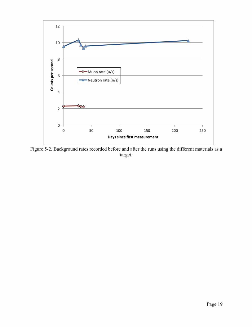
The data in Figure 5-2 show the neutron and muon background rates that were measured during the time period that most of the various target materials were being counted. Data values are listed in Table 1.2. The background neutron rate remained fairly constant at 9.6(4) counts per second and the muon rate was constant at 2.28(5) counts per second.
Page 19
Figure 5-2. Background rates recorded before and after the runs using the different materials as a
target.
0
2
4
6
8
10
12
0 50 100 150 200 250
Coun
ts per se
cond
Days since first measurement
Muon rate (u/s)
Neutron rate (n/s)
Page 20
6. Polyethylene Run
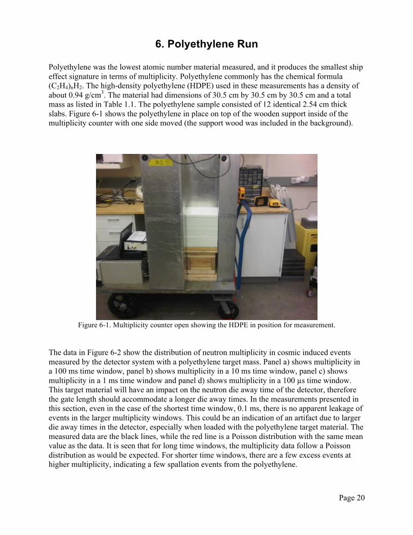
Polyethylene was the lowest atomic number material measured, and it produces the smallest ship effect signature in terms of multiplicity. Polyethylene commonly has the chemical formula (C2H4)nH2. The high-density polyethylene (HDPE) used in these measurements has a density of about 0.94 g/cm3. The material had dimensions of 30.5 cm by 30.5 cm by 30.5 cm and a total mass as listed in Table 1.1. The polyethylene sample consisted of 12 identical 2.54 cm thick slabs. Figure 6-1 shows the polyethylene in place on top of the wooden support inside of the multiplicity counter with one side moved (the support wood was included in the background).
Figure 6-1. Multiplicity counter open showing the HDPE in position for measurement.
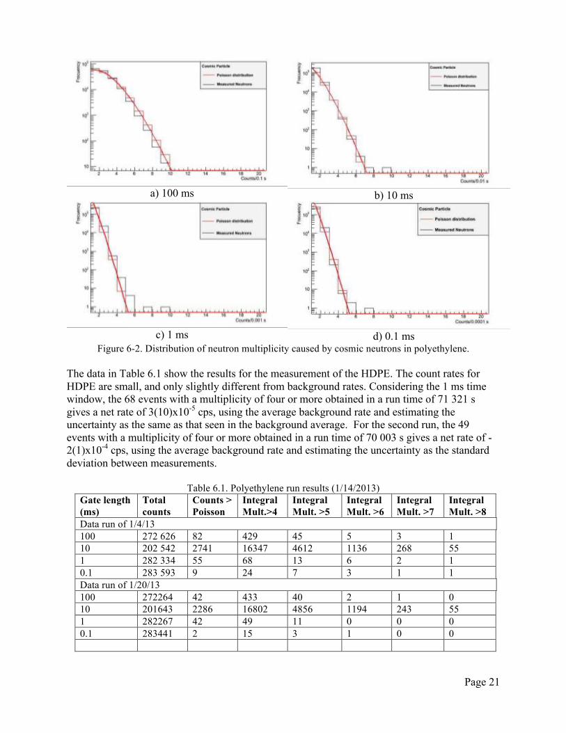
The data in Figure 6-2 show the distribution of neutron multiplicity in cosmic induced events measured by the detector system with a polyethylene target mass. Panel a) shows multiplicity in a 100 ms time window, panel b) shows multiplicity in a 10 ms time window, panel c) shows multiplicity in a 1 ms time window and panel d) shows multiplicity in a 100 µs time window. This target material will have an impact on the neutron die away time of the detector, therefore the gate length should accommodate a longer die away times. In the measurements presented in this section, even in the case of the shortest time window, 0.1 ms, there is no apparent leakage of events in the larger multiplicity windows. This could be an indication of an artifact due to larger die away times in the detector, especially when loaded with the polyethylene target material. The measured data are the black lines, while the red line is a Poisson distribution with the same mean value as the data. It is seen that for long time windows, the multiplicity data follow a Poisson distribution as would be expected. For shorter time windows, there are a few excess events at higher multiplicity, indicating a few spallation events from the polyethylene.
Page 21
a) 100 ms b) 10 ms
c) 1 ms d) 0.1 ms Figure 6-2. Distribution of neutron multiplicity caused by cosmic neutrons in polyethylene.
The data in Table 6.1 show the results for the measurement of the HDPE. The count rates for HDPE are small, and only slightly different from background rates. Considering the 1 ms time window, the 68 events with a multiplicity of four or more obtained in a run time of 71 321 s gives a net rate of 3(10)x10-5 cps, using the average background rate and estimating the uncertainty as the same as that seen in the background average. For the second run, the 49 events with a multiplicity of four or more obtained in a run time of 70 003 s gives a net rate of -2(1)x10-4 cps, using the average background rate and estimating the uncertainty as the standard deviation between measurements.
Table 6.1. Polyethylene run results (1/14/2013) Gate length (ms)
Total counts
Counts > Poisson
Integral Mult.>4
Integral Mult. >5
Integral Mult. >6
Integral Mult. >7
Integral Mult. >8
Data run of 1/4/13 100 272 626 82 429 45 5 3 1 10 202 542 2741 16347 4612 1136 268 55 1 282 334 55 68 13 6 2 1 0.1 283 593 9 24 7 3 1 1 Data run of 1/20/13 100 272264 42 433 40 2 1 0 10 201643 2286 16802 4856 1194 243 55 1 282267 42 49 11 0 0 0 0.1 283441 2 15 3 1 0 0
Page 22
7. Aluminum Run
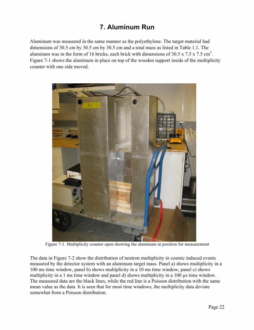
Aluminum was measured in the same manner as the polyethylene. The target material had dimensions of 30.5 cm by 30.5 cm by 30.5 cm and a total mass as listed in Table 1.1. The aluminum was in the form of 16 bricks, each brick with dimensions of 30.5 x 7.5 x 7.5 cm3. Figure 7-1 shows the aluminum in place on top of the wooden support inside of the multiplicity counter with one side moved.
Figure 7-1. Multiplicity counter open showing the aluminum in position for measurement
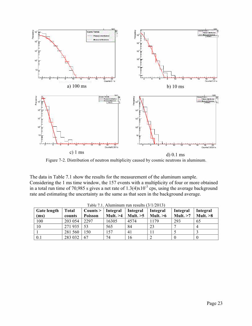
The data in Figure 7-2 show the distribution of neutron multiplicity in cosmic induced events measured by the detector system with an aluminum target mass. Panel a) shows multiplicity in a 100 ms time window, panel b) shows multiplicity in a 10 ms time window, panel c) shows multiplicity in a 1 ms time window and panel d) shows multiplicity in a 100 µs time window. The measured data are the black lines, while the red line is a Poisson distribution with the same mean value as the data. It is seen that for most time windows, the multiplicity data deviate somewhat from a Poisson distribution.
Page 23
a) 100 ms
b) 10 ms
c) 1 ms
d) 0.1 ms
Figure 7-2. Distribution of neutron multiplicity caused by cosmic neutrons in aluminum. The data in Table 7.1 show the results for the measurement of the aluminum sample. Considering the 1 ms time window, the 157 events with a multiplicity of four or more obtained in a total run time of 70,985 s gives a net rate of 1.3(4)x10-3 cps, using the average background rate and estimating the uncertainty as the same as that seen in the background average.
Table 7.1. Aluminum run results (3/1/2013) Gate length (ms)
Total counts
Counts > Poisson
Integral Mult. >4
Integral Mult. >5
Integral Mult. >6
Integral Mult. >7
Integral Mult. >8
100 203 054 2297 16305 4574 1179 293 65 10 271 935 53 565 84 23 7 4 1 281 560 150 157 41 11 5 3 0.1 283 032 67 74 16 2 0 0
Page 24
8. Steel Run
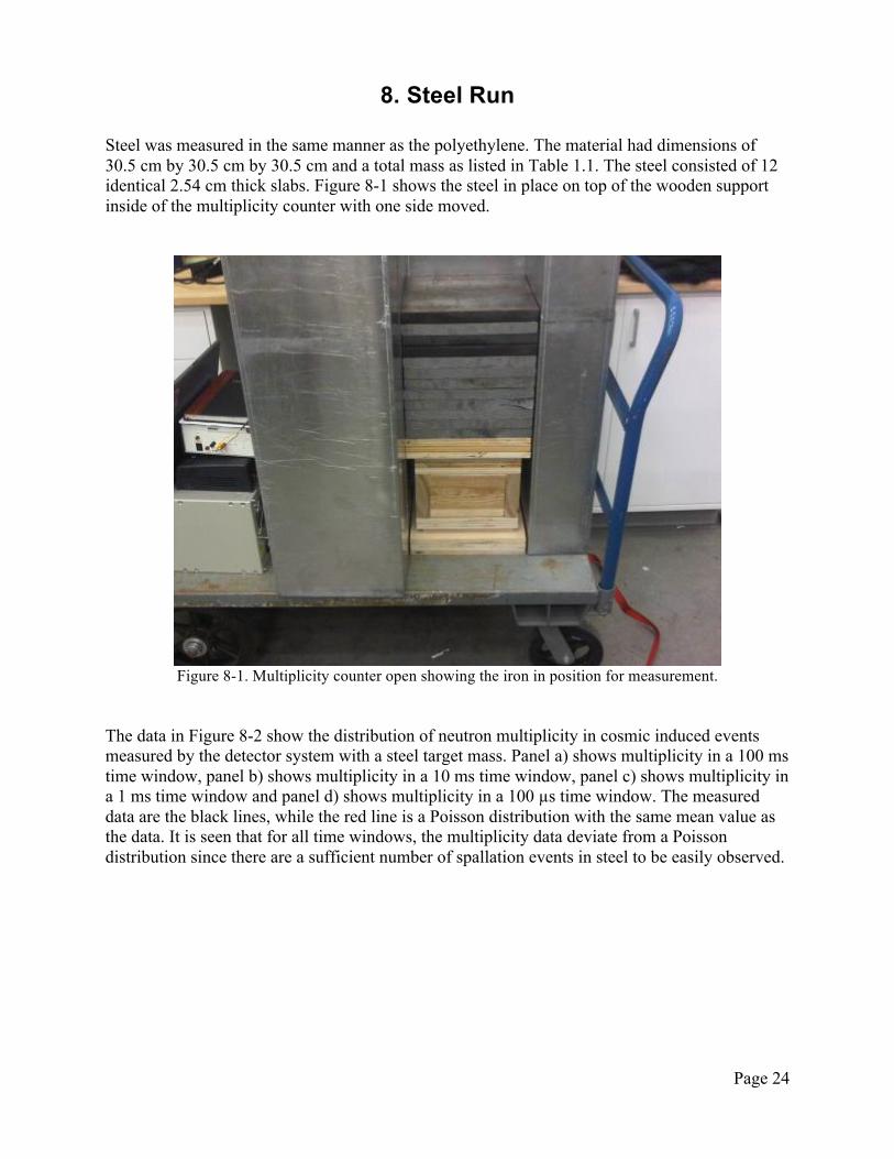
Steel was measured in the same manner as the polyethylene. The material had dimensions of 30.5 cm by 30.5 cm by 30.5 cm and a total mass as listed in Table 1.1. The steel consisted of 12 identical 2.54 cm thick slabs. Figure 8-1 shows the steel in place on top of the wooden support inside of the multiplicity counter with one side moved.
Figure 8-1. Multiplicity counter open showing the iron in position for measurement.
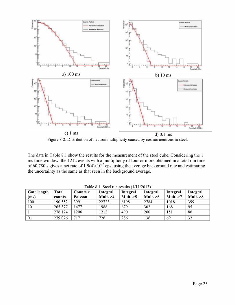
The data in Figure 8-2 show the distribution of neutron multiplicity in cosmic induced events measured by the detector system with a steel target mass. Panel a) shows multiplicity in a 100 ms time window, panel b) shows multiplicity in a 10 ms time window, panel c) shows multiplicity in a 1 ms time window and panel d) shows multiplicity in a 100 µs time window. The measured data are the black lines, while the red line is a Poisson distribution with the same mean value as the data. It is seen that for all time windows, the multiplicity data deviate from a Poisson distribution since there are a sufficient number of spallation events in steel to be easily observed.
Page 25
a) 100 ms b) 10 ms
c) 1 ms d) 0.1 ms Figure 8-2. Distribution of neutron multiplicity caused by cosmic neutrons in steel.
The data in Table 8.1 show the results for the measurement of the steel cube. Considering the 1 ms time window, the 1212 events with a multiplicity of four or more obtained in a total run time of 60,780 s gives a net rate of 1.9(4)x10-2 cps, using the average background rate and estimating the uncertainty as the same as that seen in the background average.
Table 8.1. Steel run results (1/11/2013) Gate length (ms)
Total counts
Counts > Poisson
Integral Mult. >4
Integral Mult. >5
Integral Mult. >6
Integral Mult. >7
Integral Mult. >8
100 190 552 399 22723 8198 2784 1018 399 10 265 377 1477 1988 679 302 168 95 1 276 174 1206 1212 490 260 151 86 0.1 279 076 717 726 286 136 69 32
Page 26
9. Copper Run
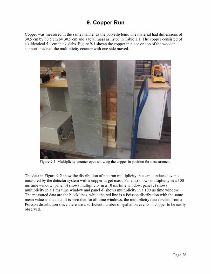
Copper was measured in the same manner as the polyethylene. The material had dimensions of 30.5 cm by 30.5 cm by 30.5 cm and a total mass as listed in Table 1.1. The copper consisted of six identical 5.1 cm thick slabs. Figure 9-1 shows the copper in place on top of the wooden support inside of the multiplicity counter with one side moved.
Figure 9-1. Multiplicity counter open showing the copper in position for measurement.
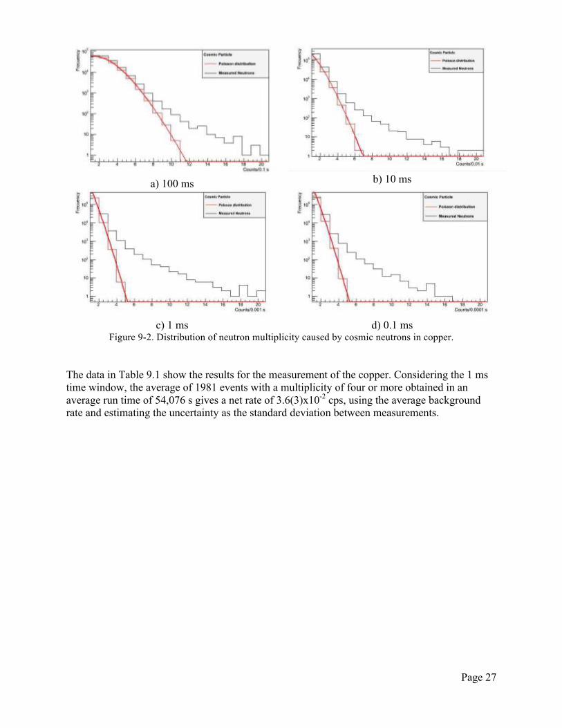
The data in Figure 9-2 show the distribution of neutron multiplicity in cosmic induced events measured by the detector system with a copper target mass. Panel a) shows multiplicity in a 100 ms time window, panel b) shows multiplicity in a 10 ms time window, panel c) shows multiplicity in a 1 ms time window and panel d) shows multiplicity in a 100 µs time window. The measured data are the black lines, while the red line is a Poisson distribution with the same mean value as the data. It is seen that for all time windows, the multiplicity data deviate from a Poisson distribution since there are a sufficient number of spallation events in copper to be easily observed.
Page 27
a) 100 ms
b) 10 ms
c) 1 ms
d) 0.1 ms
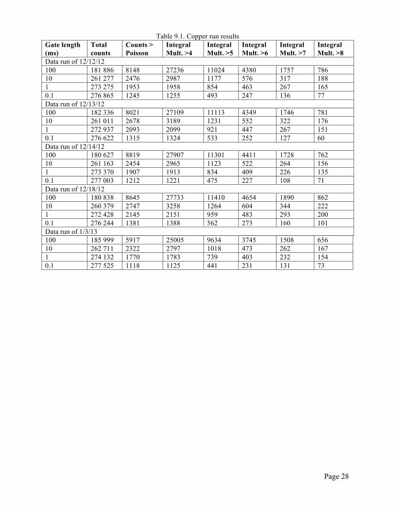
Figure 9-2. Distribution of neutron multiplicity caused by cosmic neutrons in copper. The data in Table 9.1 show the results for the measurement of the copper. Considering the 1 ms time window, the average of 1981 events with a multiplicity of four or more obtained in an average run time of 54,076 s gives a net rate of 3.6(3)x10-2 cps, using the average background rate and estimating the uncertainty as the standard deviation between measurements.
Page 28
Table 9.1. Copper run results Gate length (ms)
Total counts
Counts > Poisson
Integral Mult. >4
Integral Mult. >5
Integral Mult. >6
Integral Mult. >7
Integral Mult. >8
Data run of 12/12/12 100 181 886 8148 27236 11024 4380 1757 786 10 261 277 2476 2987 1177 576 317 188 1 273 275 1953 1958 854 463 267 165 0.1 276 865 1245 1255 493 247 136 77 Data run of 12/13/12 100 182 336 8021 27109 11113 4349 1746 781 10 261 011 2678 3189 1231 552 322 176 1 272 937 2093 2099 921 447 267 151 0.1 276 622 1315 1324 533 252 127 60 Data run of 12/14/12 100 180 627 8819 27907 11301 4411 1728 762 10 261 163 2454 2965 1123 522 264 156 1 273 370 1907 1913 834 409 226 135 0.1 277 003 1212 1221 475 227 108 71 Data run of 12/18/12 100 180 838 8645 27733 11410 4654 1890 862 10 260 379 2747 3258 1264 604 344 222 1 272 428 2145 2151 959 483 293 200 0.1 276 244 1381 1388 562 273 160 101 Data run of 1/3/13 100 185 999 5917 25005 9634 3745 1508 656 10 262 711 2322 2797 1018 473 262 167 1 274 132 1770 1783 739 403 232 154 0.1 277 525 1118 1125 441 231 131 73
Page 29
10. Lead Run
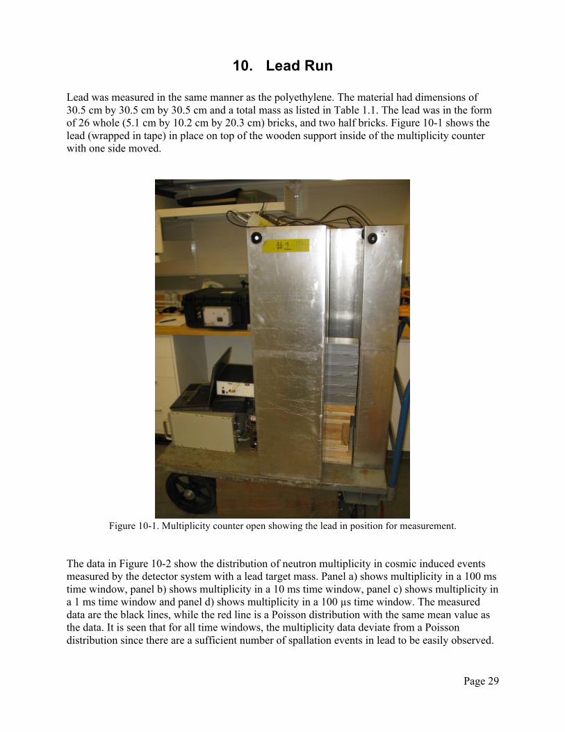
Lead was measured in the same manner as the polyethylene. The material had dimensions of 30.5 cm by 30.5 cm by 30.5 cm and a total mass as listed in Table 1.1. The lead was in the form of 26 whole (5.1 cm by 10.2 cm by 20.3 cm) bricks, and two half bricks. Figure 10-1 shows the lead (wrapped in tape) in place on top of the wooden support inside of the multiplicity counter with one side moved.
Figure 10-1. Multiplicity counter open showing the lead in position for measurement.
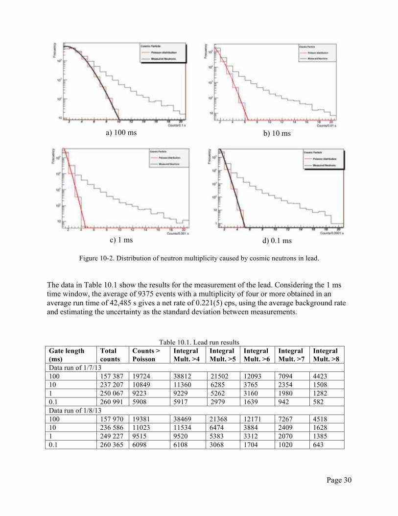
The data in Figure 10-2 show the distribution of neutron multiplicity in cosmic induced events measured by the detector system with a lead target mass. Panel a) shows multiplicity in a 100 ms time window, panel b) shows multiplicity in a 10 ms time window, panel c) shows multiplicity in a 1 ms time window and panel d) shows multiplicity in a 100 µs time window. The measured data are the black lines, while the red line is a Poisson distribution with the same mean value as the data. It is seen that for all time windows, the multiplicity data deviate from a Poisson distribution since there are a sufficient number of spallation events in lead to be easily observed.
Page 30
a) 100 ms
b) 10 ms
c) 1 ms
d) 0.1 ms
Figure 10-2. Distribution of neutron multiplicity caused by cosmic neutrons in lead.
The data in Table 10.1 show the results for the measurement of the lead. Considering the 1 ms time window, the average of 9375 events with a multiplicity of four or more obtained in an average run time of 42,485 s gives a net rate of 0.221(5) cps, using the average background rate and estimating the uncertainty as the standard deviation between measurements.
Table 10.1. Lead run results Gate length (ms)
Total counts
Counts > Poisson
Integral Mult. >4
Integral Mult. >5
Integral Mult. >6
Integral Mult. >7
Integral Mult. >8
Data run of 1/7/13 100 157 387 19724 38812 21502 12093 7094 4423 10 237 207 10849 11360 6285 3765 2354 1508 1 250 067 9223 9229 5262 3160 1980 1282 0.1 260 991 5908 5917 2979 1639 942 582 Data run of 1/8/13 100 157 970 19381 38469 21368 12171 7267 4518 10 236 586 11023 11534 6474 3884 2409 1628 1 249 227 9515 9520 5383 3312 2070 1385 0.1 260 365 6098 6108 3068 1704 1020 643
Page 31
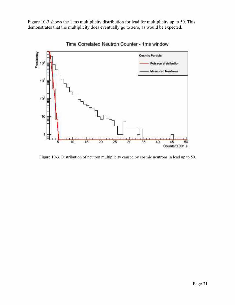
Figure 10-3 shows the 1 ms multiplicity distribution for lead for multiplicity up to 50. This demonstrates that the multiplicity does eventually go to zero, as would be expected.
Figure 10-3. Distribution of neutron multiplicity caused by cosmic neutrons in lead up to 50.
Page 32
11. Tungsten Run
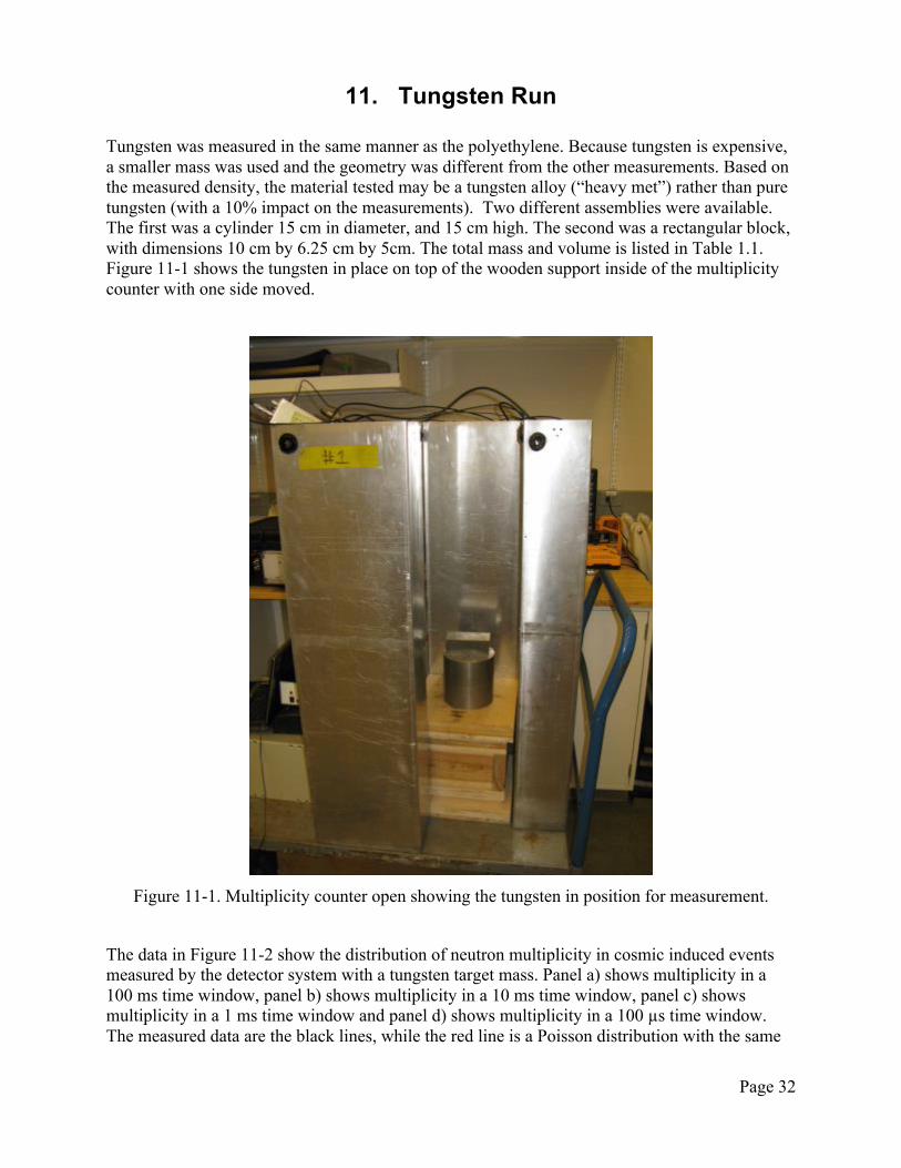
Tungsten was measured in the same manner as the polyethylene. Because tungsten is expensive, a smaller mass was used and the geometry was different from the other measurements. Based on the measured density, the material tested may be a tungsten alloy (“heavy met”) rather than pure tungsten (with a 10% impact on the measurements). Two different assemblies were available. The first was a cylinder 15 cm in diameter, and 15 cm high. The second was a rectangular block, with dimensions 10 cm by 6.25 cm by 5cm. The total mass and volume is listed in Table 1.1. Figure 11-1 shows the tungsten in place on top of the wooden support inside of the multiplicity counter with one side moved.
Figure 11-1. Multiplicity counter open showing the tungsten in position for measurement.
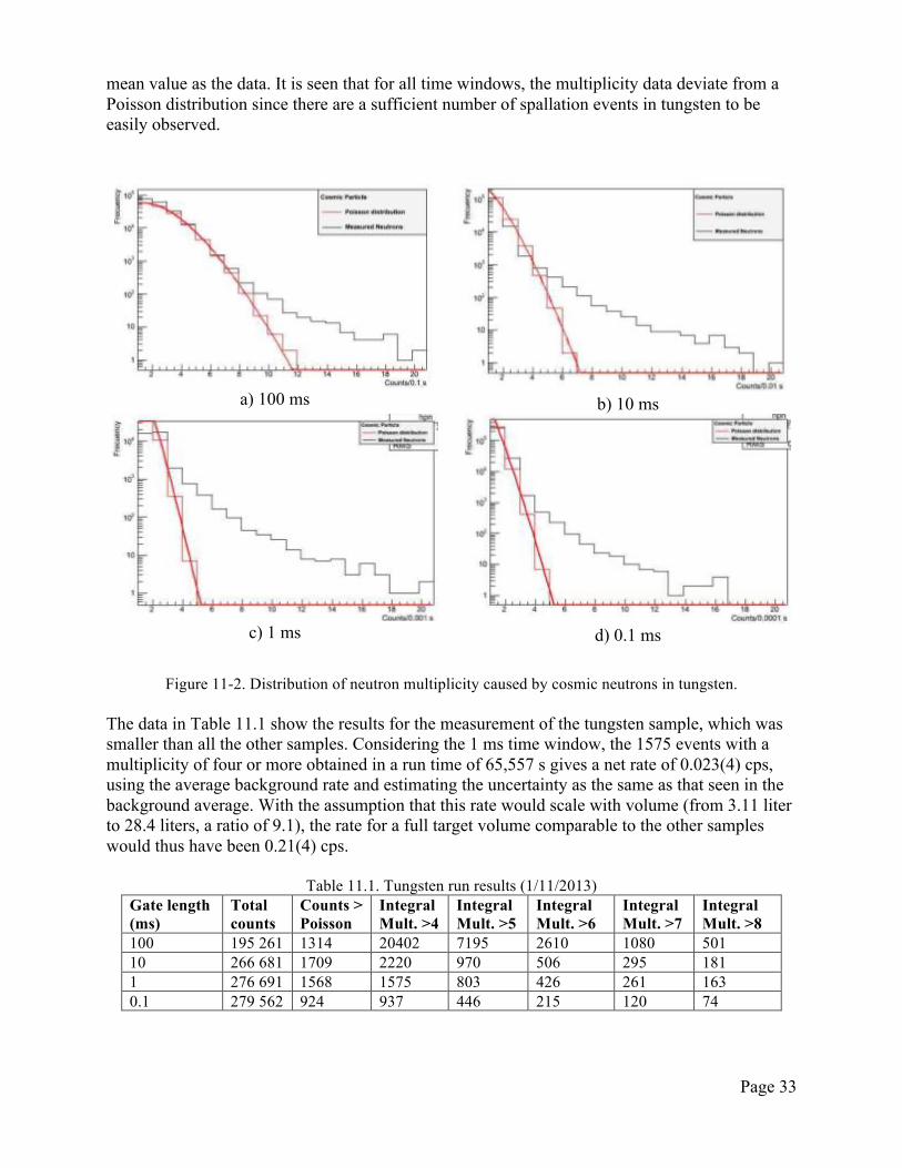
The data in Figure 11-2 show the distribution of neutron multiplicity in cosmic induced events measured by the detector system with a tungsten target mass. Panel a) shows multiplicity in a 100 ms time window, panel b) shows multiplicity in a 10 ms time window, panel c) shows multiplicity in a 1 ms time window and panel d) shows multiplicity in a 100 µs time window. The measured data are the black lines, while the red line is a Poisson distribution with the same
Page 33
mean value as the data. It is seen that for all time windows, the multiplicity data deviate from a Poisson distribution since there are a sufficient number of spallation events in tungsten to be easily observed.
a) 100 ms
b) 10 ms
c) 1 ms
d) 0.1 ms
Figure 11-2. Distribution of neutron multiplicity caused by cosmic neutrons in tungsten.
The data in Table 11.1 show the results for the measurement of the tungsten sample, which was smaller than all the other samples. Considering the 1 ms time window, the 1575 events with a multiplicity of four or more obtained in a run time of 65,557 s gives a net rate of 0.023(4) cps, using the average background rate and estimating the uncertainty as the same as that seen in the background average. With the assumption that this rate would scale with volume (from 3.11 liter to 28.4 liters, a ratio of 9.1), the rate for a full target volume comparable to the other samples would thus have been 0.21(4) cps.
Table 11.1. Tungsten run results (1/11/2013) Gate length (ms)
Total counts
Counts > Poisson
Integral Mult. >4
Integral Mult. >5
Integral Mult. >6
Integral Mult. >7
Integral Mult. >8
100 195 261 1314 20402 7195 2610 1080 501 10 266 681 1709 2220 970 506 295 181 1 276 691 1568 1575 803 426 261 163 0.1 279 562 924 937 446 215 120 74
Page 34
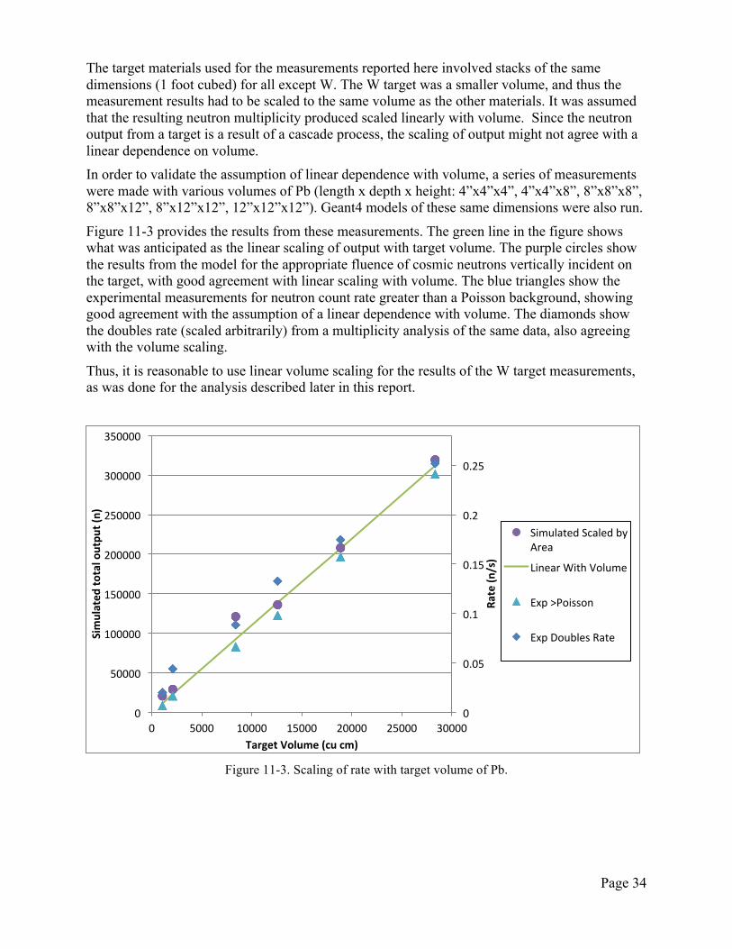
The target materials used for the measurements reported here involved stacks of the same dimensions (1 foot cubed) for all except W. The W target was a smaller volume, and thus the measurement results had to be scaled to the same volume as the other materials. It was assumed that the resulting neutron multiplicity produced scaled linearly with volume. Since the neutron output from a target is a result of a cascade process, the scaling of output might not agree with a linear dependence on volume. In order to validate the assumption of linear dependence with volume, a series of measurements were made with various volumes of Pb (length x depth x height: 4”x4”x4”, 4”x4”x8”, 8”x8”x8”, 8”x8”x12”, 8”x12”x12”, 12”x12”x12”). Geant4 models of these same dimensions were also run.
Figure 11-3 provides the results from these measurements. The green line in the figure shows what was anticipated as the linear scaling of output with target volume. The purple circles show the results from the model for the appropriate fluence of cosmic neutrons vertically incident on the target, with good agreement with linear scaling with volume. The blue triangles show the experimental measurements for neutron count rate greater than a Poisson background, showing good agreement with the assumption of a linear dependence with volume. The diamonds show the doubles rate (scaled arbitrarily) from a multiplicity analysis of the same data, also agreeing with the volume scaling.
Thus, it is reasonable to use linear volume scaling for the results of the W target measurements, as was done for the analysis described later in this report.
Figure 11-3. Scaling of rate with target volume of Pb.
0
0.05
0.1
0.15
0.2
0.25
0
50000
100000
150000
200000
250000
300000
350000
0 5000 10000 15000 20000 25000 30000
Rate (n
/s)
Simulated
total outpu
t (n)
Target Volume (cu cm)
Simulated Scaled by Area
Linear With Volume
Exp >Poisson
Exp Doubles Rate
Page 35
12. Experimental Results
The data obtained in these measurements can be analyzed in several ways by varying the time window over which events are integrated, and counting multiplicity with varying thresholds.
12.1. Integrated Experimental Multiplicity Counts
The data plotted in Figures 12-1 and Figure 12-2 show the experimental total neutron counts versus neutron density obtained from the air, polyethylene, steel, copper, lead, and tungsten samples. The lines are to guide the eye, and the uncertainties are smaller than the markers. The figures differ in the time window used for the integration of counts (10 ms versus 1 ms). The four trends of data in each figure represent counts with multiplicities greater than 5, 6, 7 and 8. The trend observed in the data is the same for all time windows.
Figure 12-1. Integrated number of events versus neutron density in 10 ms gate length.
Figure 12-2. Integrated number of events versus neutron density in 1ms gate length.
0 1000 2000 3000 4000 5000 6000 7000 8000 9000
10000
0 2 4 6
Integrated
Cou
nts
Neutron density (1024 n/cc)
10 ms Mult >5
10 ms Mult >6
10 ms Mult > 7
10 ms Mult > 8
0
1000
2000
3000
4000
5000
6000
7000
8000
0 1 2 3 4 5 6 7
Integrated
Cou
nts
Neutron density (1024 n/cc)
1 ms Mult >5
1 ms Mult >6
1 ms Mult >7
1 ms Mult >8
Page 36
The tungsten data in the plots has been scaled by volume to be comparable to the other data. As expected, the integrated counts increase with neutron density, but not in a linear fashion. While these plots use neutron density, the same trend is found when using mass density. It is more informative to convert the total counts to a rate so they can be more directly compared.
12.2. Multiplicity Rate
One way to count multiplicity is to compare results from the various materials for a selected time window with events counted above a certain multiplicity value. Table 12.1 summarizes the data analysis runs using a 1 ms time window and a multiplicity value of four or more, six or more, and eight or more, as was presented in each of the earlier sections of this report. Net rates are listed.
The table shows the density and neutron density for each of the materials, and the observed rate of events (in cps) for the fixed volume (one cubic foot) of material used in the measurements, including scaling the tungsten results to this same volume.
Table 12.1. Summary of experimental multiplicity results.
Material Density (g/cc)
Target mass (kg)
Neutron Density (n/cc x 10-24)
Rate Mult. >4
Rate Mult. >6
Rate Mult. >8
HDPE 0.95 28.05 0.25 0.0 ± 0.003
0.0 ± 0.0007
0.0 ± 0.0004
Al 2.7 76.8 0.84 0.0001 ± 0.003
0.0001 ± 0.0007
0. 0 ± 0.0004
Fe 7.87 222.6 2.54 0.019 ± 0.003
0.0042 ± 0.0007
0.0001 ± 0.0004
Cu 8.94 237.9 2.93 0.037 ± 0.003
0.0081 ± 0.0007
0.0029 ± 0.0004
Pb 11.3 320.1 4.11 0.220 ± 0.003
0.0760 ± 0.0007
0.0310 ± 0.0004
W 19.3 481.9 6.95 0.210 ± 0.003
0.0580 ± 0.0007
0.0220 ± 0.0004
This data is plotted in Figure 12-3, showing the event rate in cps versus neutron density for three multiplicity rates (4, 6 and 8). The lines are to guide the eye, and the uncertainties are smaller than the markers. The general trend is increasing event rate with neutron density, though the rate for tungsten is comparable to that of lead. There is uncertainty introduced by the volume-scaling concept used to get the tungsten rate to scale multiplicity data. There are cascade effects inside the target volume that underestimated the rate using a smaller volume of material. A Geant4 simulation was performed of the neutron output from a tungsten sample of the measured size versus a cubic foot of material. The result was a neutron yield increase by a factor of 7.1. This was somewhat smaller than the volume scaling value of 9.1, which may be within the uncertainty of the model, or may be due to attenuation in the material.
These results can be compared with previous ship effect results measured at PNNL, as shown in Figure 12-4 [Kouzes 2008]. The previous measurements had included several low density
Page 37
materials, plus iron and lead. While the trend in the new data reported here is the same as seen in the previous measurement, comparing the lead rate and iron rate in the new data to the previous results shows a significant increase in the ratio of these rates. The copper result is also lower than a linear trend would predict. Because the systematic effects are better controlled in the new experiment, these new results are thought to be more representative of the actual effect. The earlier work used a different geometry for each material measured.
Figure 12-3. Event rate versus neutron density for three multiplicities.
0
0.05
0.1
0.15
0.2
0.25
0 1 2 3 4 5 6 7
Even
t Rate
Neutron density (1024 n/cc)
Mult. > 4
Mult. > 6
Mult. > 8
Page 38
Figure 12-4. Event rate versus neutron density from [Kouzes 2008].
12.3. Reals and Accidentals Multiplicity Analysis
There is an alternative method for extracting multiplicity information to that previously discussed. The neutron multiplicity for each run can be extracted from the data by performing an analysis based on the assumption that this data contains a mixture of a “real” correlated distribution of neutrons (R) and the “accidental” (random background) distribution (A). This approach will be referred to as “R+A” analysis. Analytical expressions for the factorial moments of the neutron multiplicity distribution were used in this multiplicity analysis. The extracted rates in this analysis are the singles rate (S, multiplicity = 1), doubles rate (D, multiplicity = 2), triples rate (T, multiplicity = 3) and quadruples rate (Q, multiplicity = 4), as detailed in [Ensslin 1998]. Multiplicities above four were not computed, since the efficiency of the counter decreases rapidly and this particular data analysis yields null results. In the data presented in this section, the duration of the foreground multiplicity distribution (R+A gate) is 60 µs, and the background distribution is measured after a delay time interval (A gate) of 4 ms. This analysis method is implemented in commercially available shift registers, such as the Canberra JSR-14. In order to validate the implementation of this analysis method for the use in this work, a 252Cf neutron source measurement was made and analyzed using the VME system and a JSR-14. The results are presented in Table 12.2. The agreement in the results indicates the correct implementation of this analysis method.
Page 39
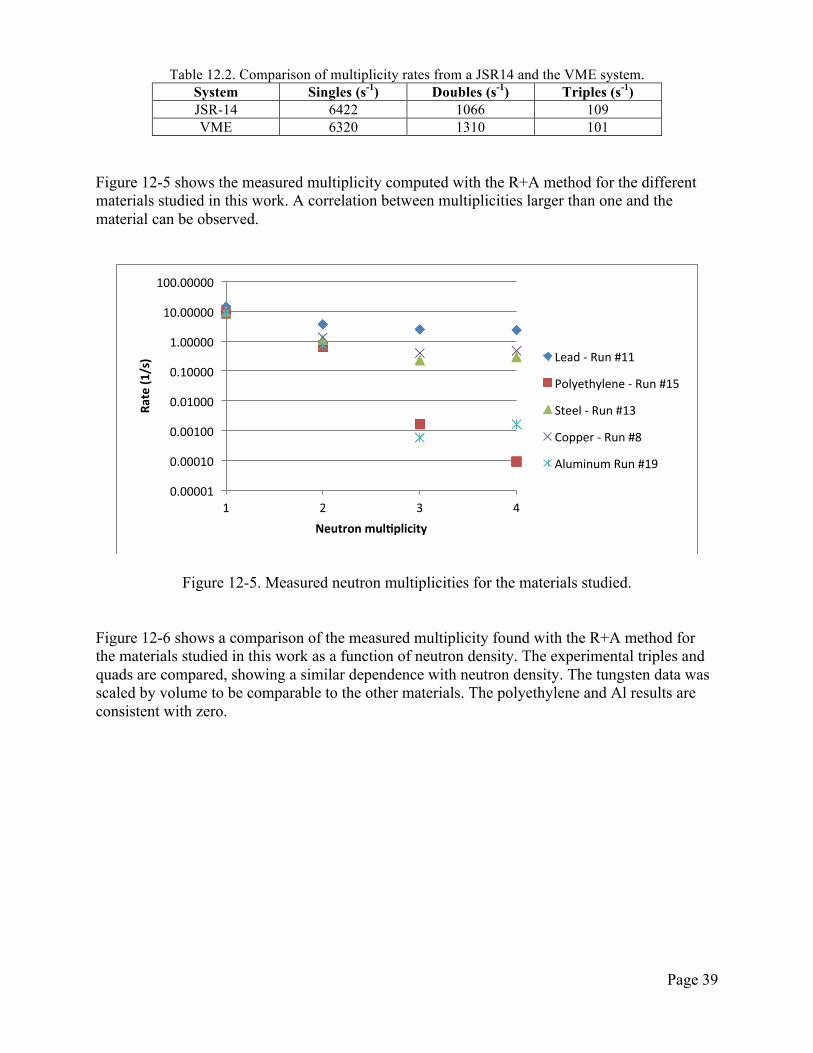
Table 12.2. Comparison of multiplicity rates from a JSR14 and the VME system. System Singles (s-1) Doubles (s-1) Triples (s-1) JSR-14 6422 1066 109 VME 6320 1310 101
Figure 12-5 shows the measured multiplicity computed with the R+A method for the different materials studied in this work. A correlation between multiplicities larger than one and the material can be observed.
Figure 12-5. Measured neutron multiplicities for the materials studied.
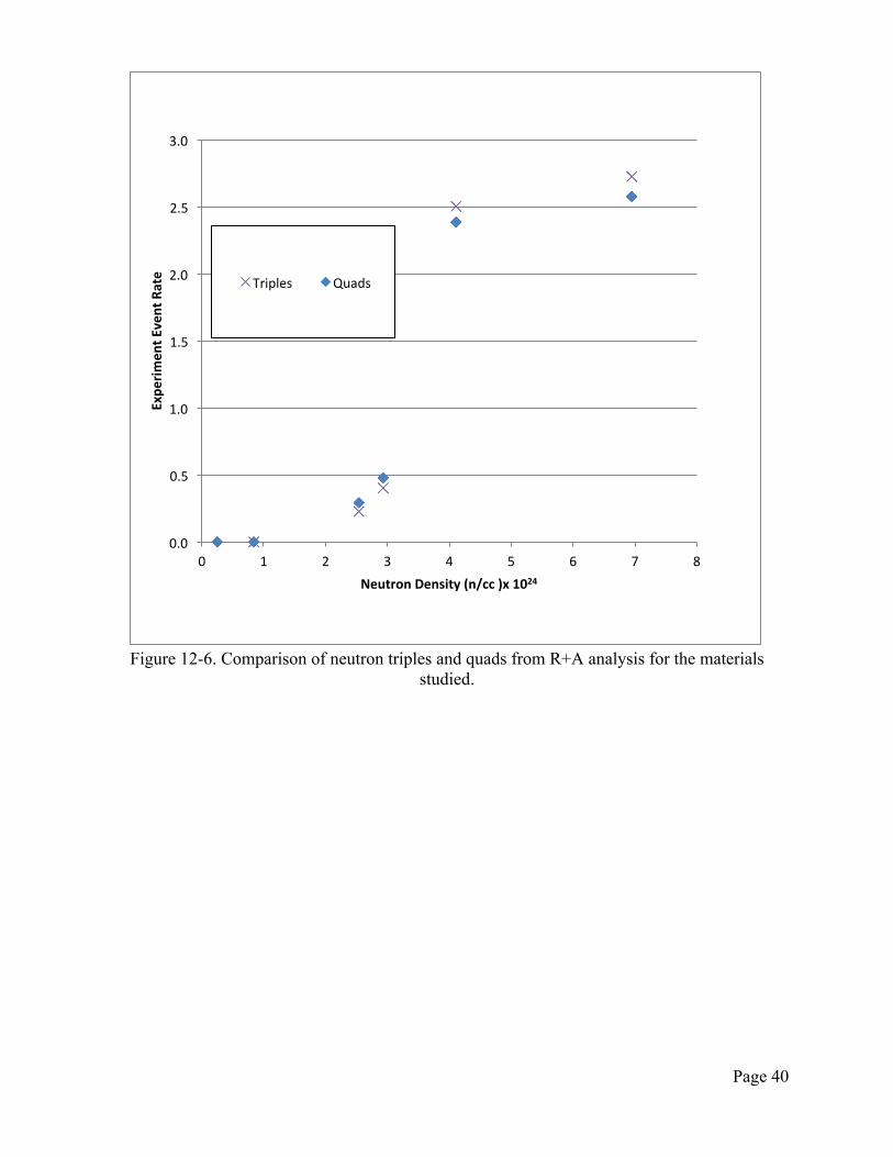
Figure 12-6 shows a comparison of the measured multiplicity found with the R+A method for the materials studied in this work as a function of neutron density. The experimental triples and quads are compared, showing a similar dependence with neutron density. The tungsten data was scaled by volume to be comparable to the other materials. The polyethylene and Al results are consistent with zero.
0.00001
0.00010
0.00100
0.01000
0.10000
1.00000
10.00000
100.00000
1 2 3 4
Rate (1
/s)
Neutron mul'plicity
Lead -‐ Run #11
Polyethylene -‐ Run #15
Steel -‐ Run #13
Copper -‐ Run #8
Aluminum Run #19
Page 40
Figure 12-6. Comparison of neutron triples and quads from R+A analysis for the materials
studied.
0.0
0.5
1.0
1.5
2.0
2.5
3.0
0 1 2 3 4 5 6 7 8
Expe
rimen
t Event Rate
Neutron Density (n/cc )x 1024
Triples Quads
Page 41
13. Geant4 Monte Carlo Modeling
A Monte Carlo model was developed to compare to the measured experimental trend. The simulation is intended to evaluate the neutron physics within the model code and therefore was kept very simple to avoid incorporating other effects, such as neutron detector efficiency, into the simulation. Thus, the model is to predict the relative response of materials, not the absolute response. Monte Carlo modeling was performed using Geant4 [Geant4 2011]. The complete details of the simulation method are given in a previous report [Aguayo 2011]. For the cosmic neutron spectrum at sea level, the model results utilize the Gordon-Goldhagen [Gordon 2004] parameterization of the cosmic ray shower, though a comparison with other spectra was also made.
13.1. Geant4 Multiplicity Results
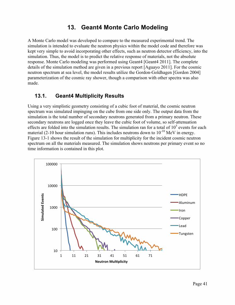
Using a very simplistic geometry consisting of a cubic foot of material, the cosmic neutron spectrum was simulated impinging on the cube from one side only. The output data from the simulation is the total number of secondary neutrons generated from a primary neutron. These secondary neutrons are logged once they leave the cubic foot of volume, so self-attenuation effects are folded into the simulation results. The simulation ran for a total of 105 events for each material (2-10 hour simulation runs). This includes neutrons down to 10-10 MeV in energy. Figure 13-1 shows the result of the simulation for multiplicity for the incident cosmic neutron spectrum on all the materials measured. The simulation shows neutrons per primary event so no time information is contained in this plot.
10
100
1000
10000
100000
1 11 21 31 41 51 61 71
Simulated
Events
Neutron Mul'plicity
HDPE
Aluminum
Iron
Copper
Lead
Tungsten
Page 42
Figure 13-1. Cosmic neutron simulation results for the materials studied.
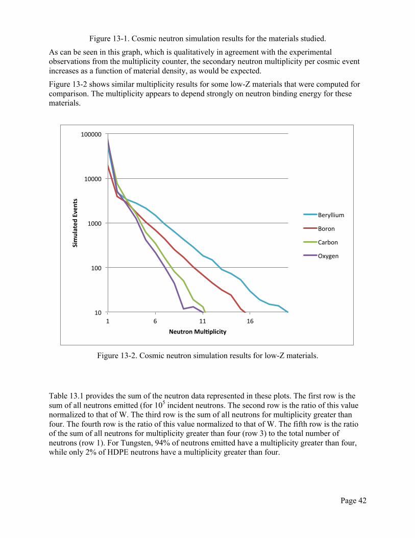
As can be seen in this graph, which is qualitatively in agreement with the experimental observations from the multiplicity counter, the secondary neutron multiplicity per cosmic event increases as a function of material density, as would be expected. Figure 13-2 shows similar multiplicity results for some low-Z materials that were computed for comparison. The multiplicity appears to depend strongly on neutron binding energy for these materials.
Figure 13-2. Cosmic neutron simulation results for low-Z materials.
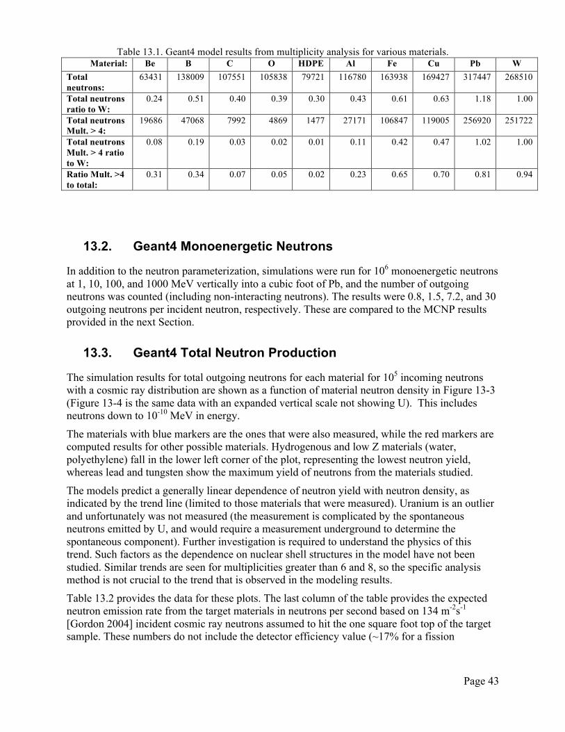
Table 13.1 provides the sum of the neutron data represented in these plots. The first row is the sum of all neutrons emitted (for 105 incident neutrons. The second row is the ratio of this value normalized to that of W. The third row is the sum of all neutrons for multiplicity greater than four. The fourth row is the ratio of this value normalized to that of W. The fifth row is the ratio of the sum of all neutrons for multiplicity greater than four (row 3) to the total number of neutrons (row 1). For Tungsten, 94% of neutrons emitted have a multiplicity greater than four, while only 2% of HDPE neutrons have a multiplicity greater than four.
10
100
1000
10000
100000
1 6 11 16
Simulated
Events
Neutron Mul'plicity
Beryllium
Boron
Carbon
Oxygen
Page 43
Table 13.1. Geant4 model results from multiplicity analysis for various materials. Material: Be B C O HDPE Al Fe Cu Pb W
Total neutrons:
63431 138009 107551 105838 79721 116780 163938 169427 317447 268510
Total neutrons ratio to W:
0.24 0.51 0.40 0.39 0.30 0.43 0.61 0.63 1.18 1.00
Total neutrons Mult. > 4:
19686 47068 7992 4869 1477 27171 106847 119005 256920 251722
Total neutrons Mult. > 4 ratio to W:
0.08 0.19 0.03 0.02 0.01 0.11 0.42 0.47 1.02 1.00
Ratio Mult. >4 to total:
0.31 0.34 0.07 0.05 0.02 0.23 0.65 0.70 0.81 0.94
13.2. Geant4 Monoenergetic Neutrons
In addition to the neutron parameterization, simulations were run for 106 monoenergetic neutrons at 1, 10, 100, and 1000 MeV vertically into a cubic foot of Pb, and the number of outgoing neutrons was counted (including non-interacting neutrons). The results were 0.8, 1.5, 7.2, and 30 outgoing neutrons per incident neutron, respectively. These are compared to the MCNP results provided in the next Section.
13.3. Geant4 Total Neutron Production
The simulation results for total outgoing neutrons for each material for 105 incoming neutrons with a cosmic ray distribution are shown as a function of material neutron density in Figure 13-3 (Figure 13-4 is the same data with an expanded vertical scale not showing U). This includes neutrons down to 10-10 MeV in energy.
The materials with blue markers are the ones that were also measured, while the red markers are computed results for other possible materials. Hydrogenous and low Z materials (water, polyethylene) fall in the lower left corner of the plot, representing the lowest neutron yield, whereas lead and tungsten show the maximum yield of neutrons from the materials studied.
The models predict a generally linear dependence of neutron yield with neutron density, as indicated by the trend line (limited to those materials that were measured). Uranium is an outlier and unfortunately was not measured (the measurement is complicated by the spontaneous neutrons emitted by U, and would require a measurement underground to determine the spontaneous component). Further investigation is required to understand the physics of this trend. Such factors as the dependence on nuclear shell structures in the model have not been studied. Similar trends are seen for multiplicities greater than 6 and 8, so the specific analysis method is not crucial to the trend that is observed in the modeling results.
Table 13.2 provides the data for these plots. The last column of the table provides the expected neutron emission rate from the target materials in neutrons per second based on 134 m-2s-1 [Gordon 2004] incident cosmic ray neutrons assumed to hit the one square foot top of the target sample. These numbers do not include the detector efficiency value (~17% for a fission
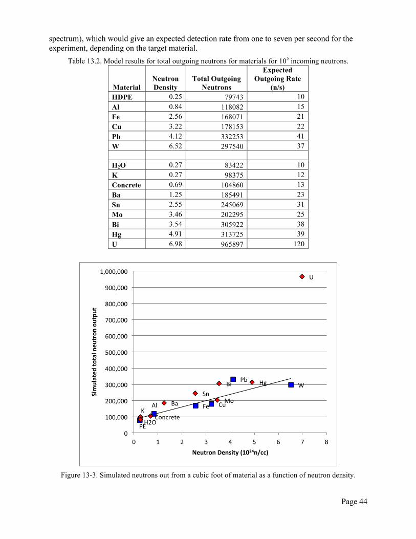
Page 44
spectrum), which would give an expected detection rate from one to seven per second for the experiment, depending on the target material.
Table 13.2. Model results for total outgoing neutrons for materials for 105 incoming neutrons.
Material Neutron Density
Total Outgoing Neutrons
Expected Outgoing Rate
(n/s) HDPE 0.25 79743 10 Al 0.84 118082 15 Fe 2.56 168071 21 Cu 3.22 178153 22 Pb 4.12 332253 41 W 6.52 297540 37 H2O 0.27 83422 10 K 0.27 98375 12 Concrete 0.69 104860 13 Ba 1.25 185491 23 Sn 2.55 245069 31 Mo 3.46 202295 25 Bi 3.54 305922 38 Hg 4.91 313725 39 U 6.98 965897 120
Figure 13-3. Simulated neutrons out from a cubic foot of material as a function of neutron density.
PE
Fe
Pb W
Cu Al K
Bi Hg
Mo Sn
Ba
U
H2O Concrete
0
100,000
200,000
300,000
400,000
500,000
600,000
700,000
800,000
900,000
1,000,000
0 1 2 3 4 5 6 7 8
Simulated
total neu
tron
outpu
t
Neutron Density (1024n/cc)
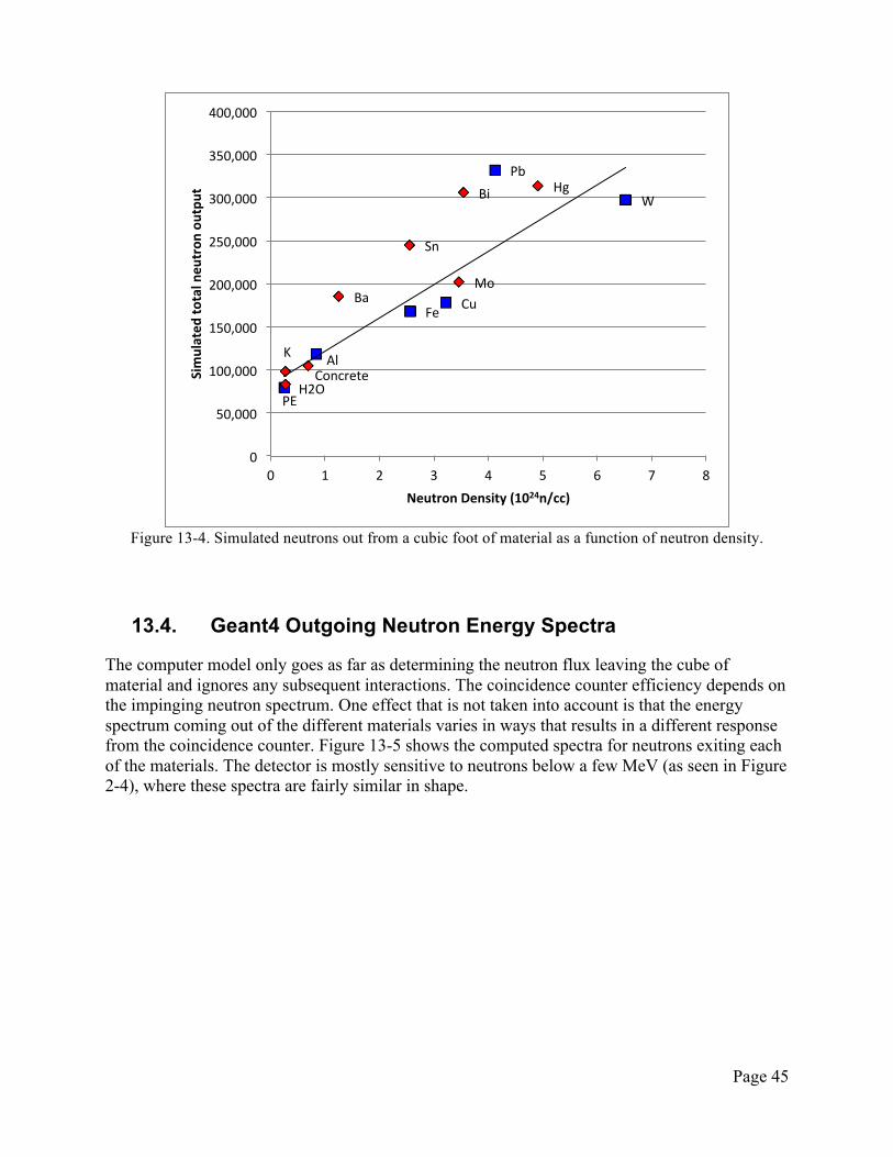
Page 45
Figure 13-4. Simulated neutrons out from a cubic foot of material as a function of neutron density.
13.4. Geant4 Outgoing Neutron Energy Spectra
The computer model only goes as far as determining the neutron flux leaving the cube of material and ignores any subsequent interactions. The coincidence counter efficiency depends on the impinging neutron spectrum. One effect that is not taken into account is that the energy spectrum coming out of the different materials varies in ways that results in a different response from the coincidence counter. Figure 13-5 shows the computed spectra for neutrons exiting each of the materials. The detector is mostly sensitive to neutrons below a few MeV (as seen in Figure 2-4), where these spectra are fairly similar in shape.
PE
Fe
Pb
W
Cu
Al K
Bi Hg
Mo
Sn
Ba
H2O Concrete
0
50,000
100,000
150,000
200,000
250,000
300,000
350,000
400,000
0 1 2 3 4 5 6 7 8
Simulated
total neu
tron
outpu
t
Neutron Density (1024n/cc)
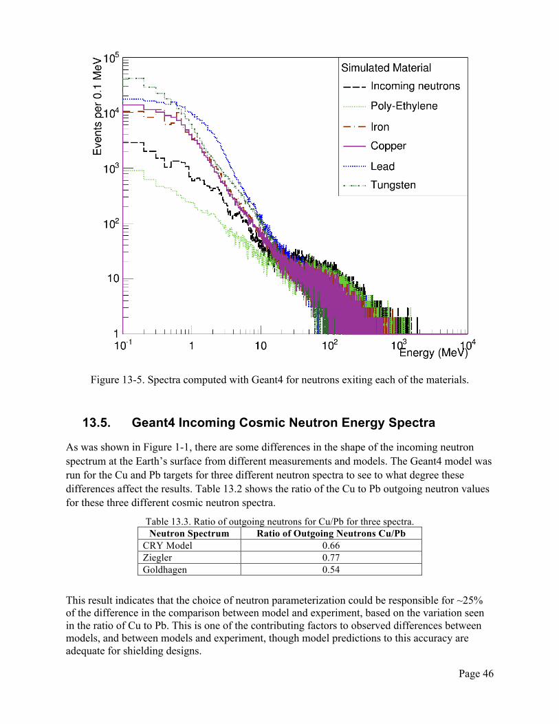
Page 46
Figure 13-5. Spectra computed with Geant4 for neutrons exiting each of the materials.
13.5. Geant4 Incoming Cosmic Neutron Energy Spectra
As was shown in Figure 1-1, there are some differences in the shape of the incoming neutron spectrum at the Earth’s surface from different measurements and models. The Geant4 model was run for the Cu and Pb targets for three different neutron spectra to see to what degree these differences affect the results. Table 13.2 shows the ratio of the Cu to Pb outgoing neutron values for these three different cosmic neutron spectra.
Table 13.3. Ratio of outgoing neutrons for Cu/Pb for three spectra. Neutron Spectrum Ratio of Outgoing Neutrons Cu/Pb
CRY Model 0.66 Ziegler 0.77 Goldhagen 0.54
This result indicates that the choice of neutron parameterization could be responsible for ~25% of the difference in the comparison between model and experiment, based on the variation seen in the ratio of Cu to Pb. This is one of the contributing factors to observed differences between models, and between models and experiment, though model predictions to this accuracy are adequate for shielding designs.
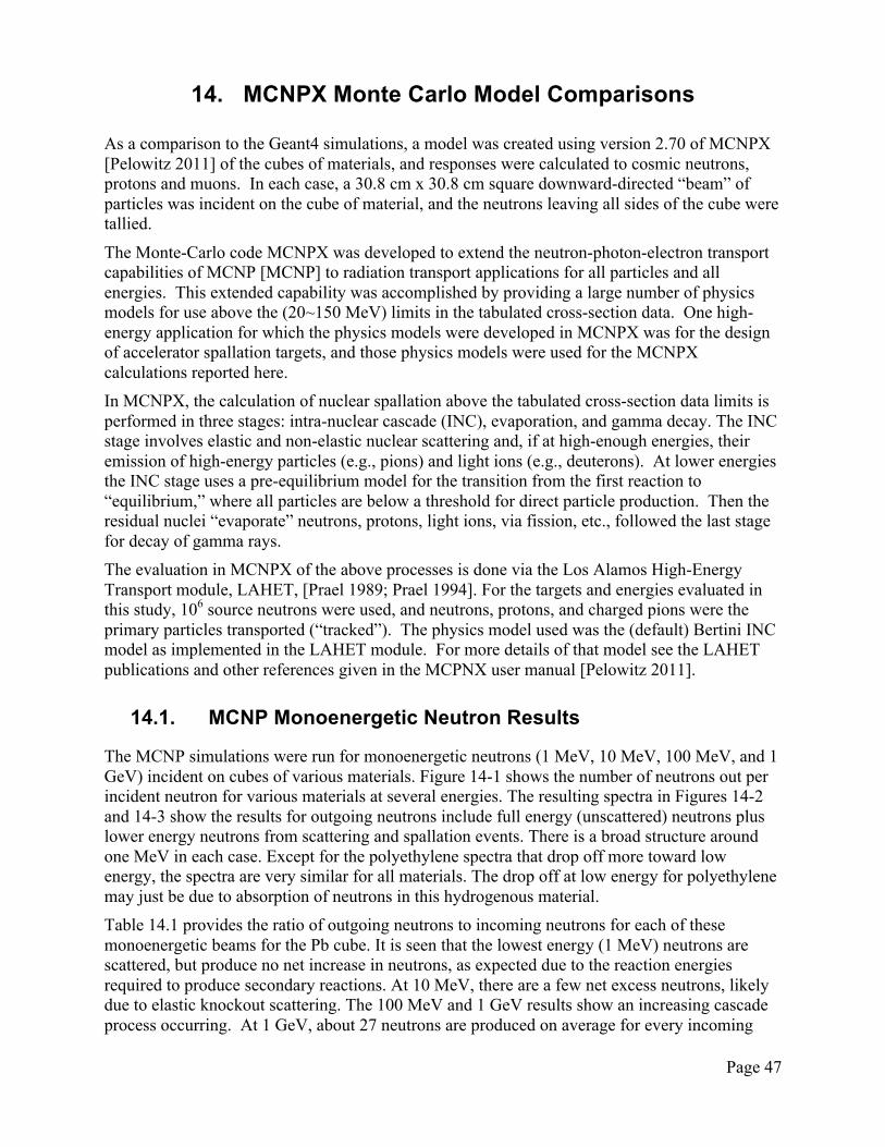
Page 47
14. MCNPX Monte Carlo Model Comparisons
As a comparison to the Geant4 simulations, a model was created using version 2.70 of MCNPX [Pelowitz 2011] of the cubes of materials, and responses were calculated to cosmic neutrons, protons and muons. In each case, a 30.8 cm x 30.8 cm square downward-directed “beam” of particles was incident on the cube of material, and the neutrons leaving all sides of the cube were tallied.
The Monte-Carlo code MCNPX was developed to extend the neutron-photon-electron transport capabilities of MCNP [MCNP] to radiation transport applications for all particles and all energies. This extended capability was accomplished by providing a large number of physics models for use above the (20~150 MeV) limits in the tabulated cross-section data. One high-energy application for which the physics models were developed in MCNPX was for the design of accelerator spallation targets, and those physics models were used for the MCNPX calculations reported here. In MCNPX, the calculation of nuclear spallation above the tabulated cross-section data limits is performed in three stages: intra-nuclear cascade (INC), evaporation, and gamma decay. The INC stage involves elastic and non-elastic nuclear scattering and, if at high-enough energies, their emission of high-energy particles (e.g., pions) and light ions (e.g., deuterons). At lower energies the INC stage uses a pre-equilibrium model for the transition from the first reaction to “equilibrium,” where all particles are below a threshold for direct particle production. Then the residual nuclei “evaporate” neutrons, protons, light ions, via fission, etc., followed the last stage for decay of gamma rays. The evaluation in MCNPX of the above processes is done via the Los Alamos High-Energy Transport module, LAHET, [Prael 1989; Prael 1994]. For the targets and energies evaluated in this study, 106 source neutrons were used, and neutrons, protons, and charged pions were the primary particles transported (“tracked”). The physics model used was the (default) Bertini INC model as implemented in the LAHET module. For more details of that model see the LAHET publications and other references given in the MCPNX user manual [Pelowitz 2011].
14.1. MCNP Monoenergetic Neutron Results
The MCNP simulations were run for monoenergetic neutrons (1 MeV, 10 MeV, 100 MeV, and 1 GeV) incident on cubes of various materials. Figure 14-1 shows the number of neutrons out per incident neutron for various materials at several energies. The resulting spectra in Figures 14-2 and 14-3 show the results for outgoing neutrons include full energy (unscattered) neutrons plus lower energy neutrons from scattering and spallation events. There is a broad structure around one MeV in each case. Except for the polyethylene spectra that drop off more toward low energy, the spectra are very similar for all materials. The drop off at low energy for polyethylene may just be due to absorption of neutrons in this hydrogenous material. Table 14.1 provides the ratio of outgoing neutrons to incoming neutrons for each of these monoenergetic beams for the Pb cube. It is seen that the lowest energy (1 MeV) neutrons are scattered, but produce no net increase in neutrons, as expected due to the reaction energies required to produce secondary reactions. At 10 MeV, there are a few net excess neutrons, likely due to elastic knockout scattering. The 100 MeV and 1 GeV results show an increasing cascade process occurring. At 1 GeV, about 27 neutrons are produced on average for every incoming
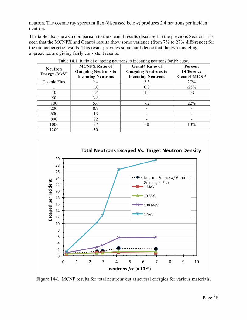
Page 48
neutron. The cosmic ray spectrum flux (discussed below) produces 2.4 neutrons per incident neutron. The table also shows a comparison to the Geant4 results discussed in the previous Section. It is seen that the MCNPX and Geant4 results show some variance (from 7% to 27% difference) for the monoenergetic results. This result provides some confidence that the two modeling approaches are giving fairly consistent results.
Table 14.1. Ratio of outgoing neutrons to incoming neutrons for Pb cube.
Neutron Energy (MeV)
MCNPX Ratio of Outgoing Neutrons to
Incoming Neutrons
Geant4 Ratio of Outgoing Neutrons to
Incoming Neutrons
Percent Difference
Geant4-MCNP Cosmic Flux 2.4 3.3 27%
1 1.0 0.8 -25% 10 1.4 1.5 7% 50 3.8 - -
100 5.6 7.2 22% 200 8.7 - - 600 13 - - 800 22 - -
1000 27 30 10% 1200 30 - -
Figure 14-1. MCNP results for total neutrons out at several energies for various materials.
0
2
4
6
8
10
12
14
16
18
20
22
24
26
28
30
0 1 2 3 4 5 6 7 8 9 10
Escape
d pe
r Inciden
t
neutrons /cc (x 10-‐24)
Total Neutrons Escaped Vs. Target Neutron Density
Neutron Source w/ Gordon-‐Goldhagen Flux 1 MeV
10 MeV
100 MeV
1 GeV
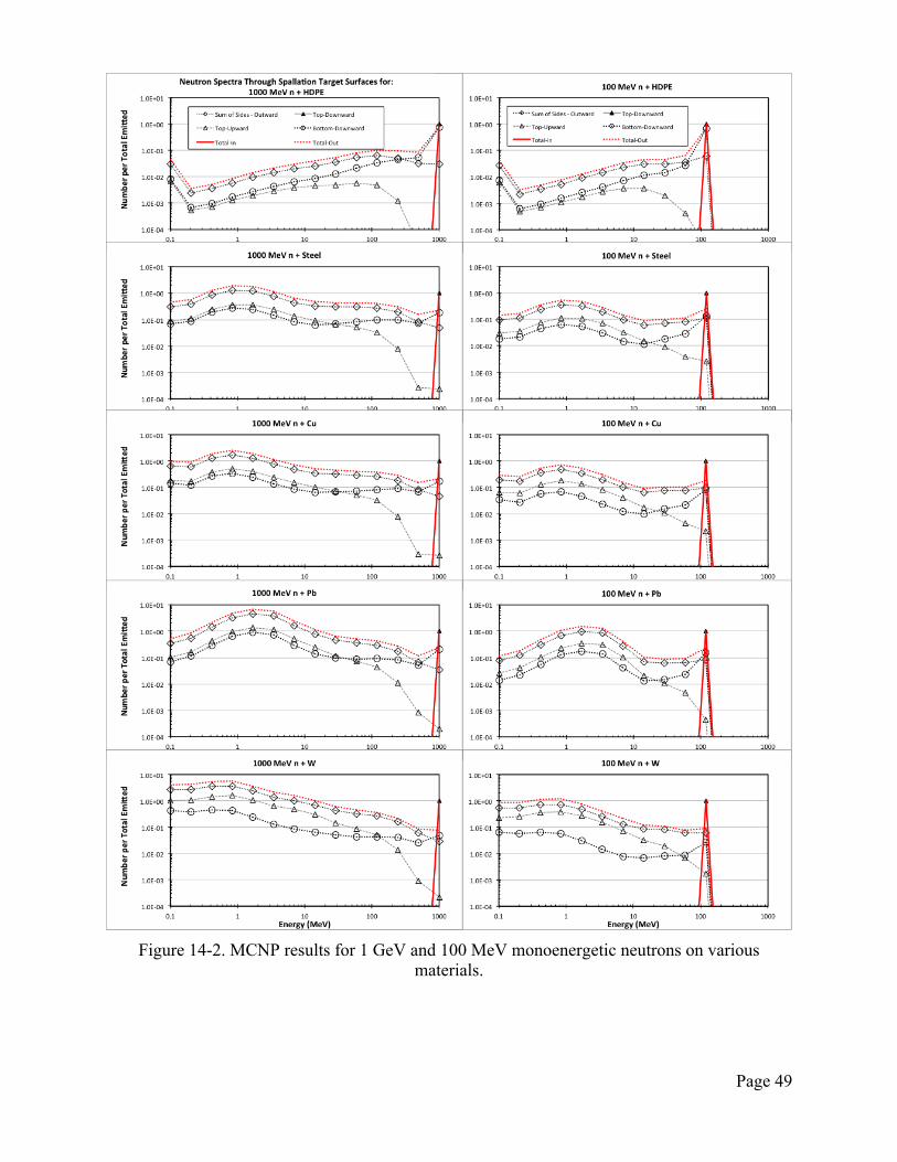
Page 49
Figure 14-2. MCNP results for 1 GeV and 100 MeV monoenergetic neutrons on various
materials.
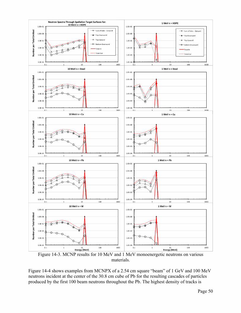
Page 50
Figure 14-3. MCNP results for 10 MeV and 1 MeV monoenergetic neutrons on various
materials. Figure 14-4 shows examples from MCNPX of a 2.54 cm square “beam” of 1 GeV and 100 MeV neutrons incident at the center of the 30.8 cm cube of Pb for the resulting cascades of particles produced by the first 100 beam neutrons throughout the Pb. The highest density of tracks is
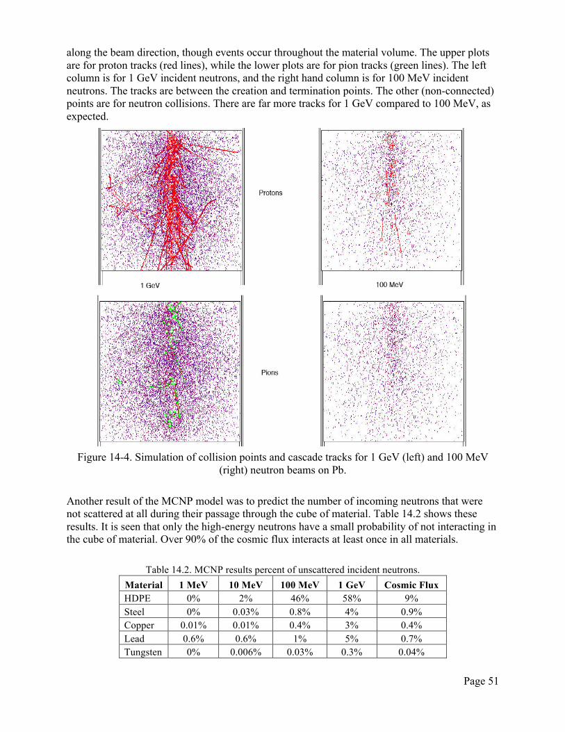
Page 51
along the beam direction, though events occur throughout the material volume. The upper plots are for proton tracks (red lines), while the lower plots are for pion tracks (green lines). The left column is for 1 GeV incident neutrons, and the right hand column is for 100 MeV incident neutrons. The tracks are between the creation and termination points. The other (non-connected) points are for neutron collisions. There are far more tracks for 1 GeV compared to 100 MeV, as expected.
Figure 14-4. Simulation of collision points and cascade tracks for 1 GeV (left) and 100 MeV
(right) neutron beams on Pb.
Another result of the MCNP model was to predict the number of incoming neutrons that were not scattered at all during their passage through the cube of material. Table 14.2 shows these results. It is seen that only the high-energy neutrons have a small probability of not interacting in the cube of material. Over 90% of the cosmic flux interacts at least once in all materials.
Table 14.2. MCNP results percent of unscattered incident neutrons.
Material 1 MeV 10 MeV 100 MeV 1 GeV Cosmic Flux HDPE 0% 2% 46% 58% 9% Steel 0% 0.03% 0.8% 4% 0.9% Copper 0.01% 0.01% 0.4% 3% 0.4% Lead 0.6% 0.6% 1% 5% 0.7% Tungsten 0% 0.006% 0.03% 0.3% 0.04%
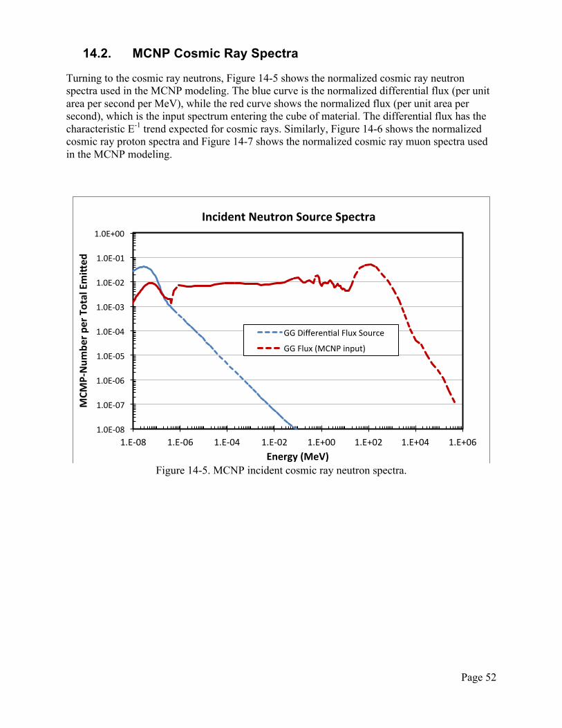
Page 52
14.2. MCNP Cosmic Ray Spectra
Turning to the cosmic ray neutrons, Figure 14-5 shows the normalized cosmic ray neutron spectra used in the MCNP modeling. The blue curve is the normalized differential flux (per unit area per second per MeV), while the red curve shows the normalized flux (per unit area per second), which is the input spectrum entering the cube of material. The differential flux has the characteristic E-1 trend expected for cosmic rays. Similarly, Figure 14-6 shows the normalized cosmic ray proton spectra and Figure 14-7 shows the normalized cosmic ray muon spectra used in the MCNP modeling.
Figure 14-5. MCNP incident cosmic ray neutron spectra.
1.0E-‐08
1.0E-‐07
1.0E-‐06
1.0E-‐05
1.0E-‐04
1.0E-‐03
1.0E-‐02
1.0E-‐01
1.0E+00
1.E-‐08 1.E-‐06 1.E-‐04 1.E-‐02 1.E+00 1.E+02 1.E+04 1.E+06
MCM
P-‐Num
ber p
er Total EmiMed
Energy (MeV)
Incident Neutron Source Spectra
GG Differenbal Flux Source
GG Flux (MCNP input)
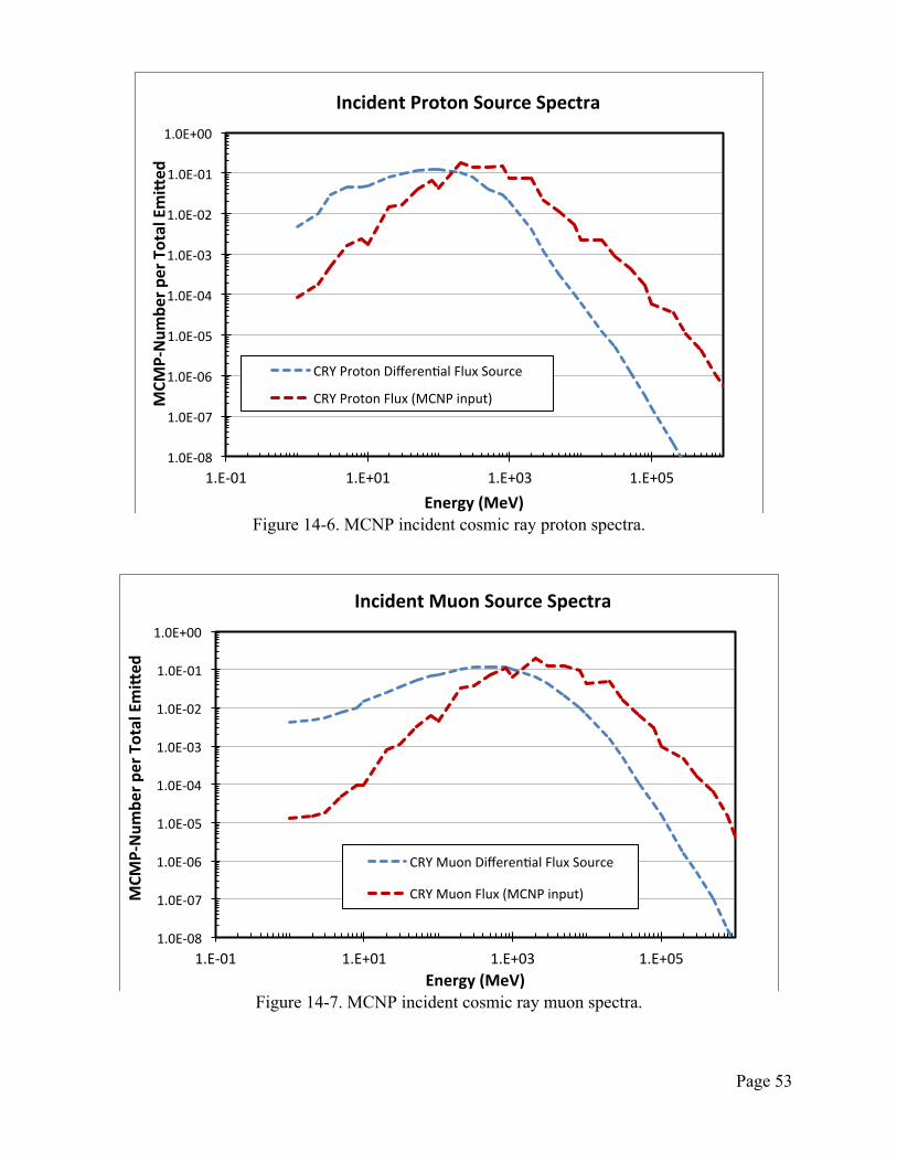
Page 53
Figure 14-6. MCNP incident cosmic ray proton spectra.
Figure 14-7. MCNP incident cosmic ray muon spectra.
1.0E-‐08
1.0E-‐07
1.0E-‐06
1.0E-‐05
1.0E-‐04
1.0E-‐03
1.0E-‐02
1.0E-‐01
1.0E+00
1.E-‐01 1.E+01 1.E+03 1.E+05
MCM
P-‐Num
ber p
er Total EmiMed
Energy (MeV)
Incident Proton Source Spectra
CRY Proton Differenbal Flux Source
CRY Proton Flux (MCNP input)
1.0E-‐08
1.0E-‐07
1.0E-‐06
1.0E-‐05
1.0E-‐04
1.0E-‐03
1.0E-‐02
1.0E-‐01
1.0E+00
1.E-‐01 1.E+01 1.E+03 1.E+05
MCM
P-‐Num
ber p
er Total EmiMed
Energy (MeV)
Incident Muon Source Spectra
CRY Muon Differenbal Flux Source
CRY Muon Flux (MCNP input)
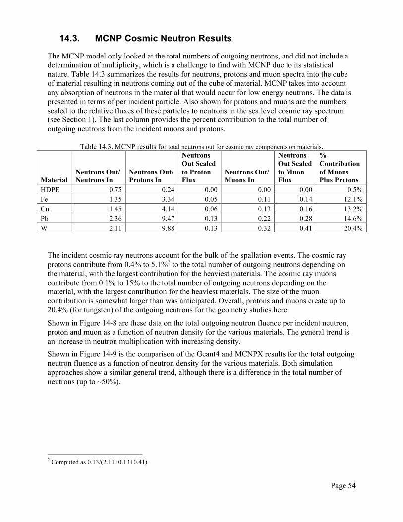
Page 54
14.3. MCNP Cosmic Neutron Results
The MCNP model only looked at the total numbers of outgoing neutrons, and did not include a determination of multiplicity, which is a challenge to find with MCNP due to its statistical nature. Table 14.3 summarizes the results for neutrons, protons and muon spectra into the cube of material resulting in neutrons coming out of the cube of material. MCNP takes into account any absorption of neutrons in the material that would occur for low energy neutrons. The data is presented in terms of per incident particle. Also shown for protons and muons are the numbers scaled to the relative fluxes of these particles to neutrons in the sea level cosmic ray spectrum (see Section 1). The last column provides the percent contribution to the total number of outgoing neutrons from the incident muons and protons.
Table 14.3. MCNP results for total neutrons out for cosmic ray components on materials.
Material Neutrons Out/ Neutrons In
Neutrons Out/ Protons In
Neutrons Out Scaled to Proton Flux
Neutrons Out/ Muons In
Neutrons Out Scaled to Muon Flux
% Contribution of Muons Plus Protons
HDPE 0.75 0.24 0.00 0.00 0.00 0.5% Fe 1.35 3.34 0.05 0.11 0.14 12.1% Cu 1.45 4.14 0.06 0.13 0.16 13.2% Pb 2.36 9.47 0.13 0.22 0.28 14.6% W 2.11 9.88 0.13 0.32 0.41 20.4%
The incident cosmic ray neutrons account for the bulk of the spallation events. The cosmic ray protons contribute from 0.4% to 5.1%2 to the total number of outgoing neutrons depending on the material, with the largest contribution for the heaviest materials. The cosmic ray muons contribute from 0.1% to 15% to the total number of outgoing neutrons depending on the material, with the largest contribution for the heaviest materials. The size of the muon contribution is somewhat larger than was anticipated. Overall, protons and muons create up to 20.4% (for tungsten) of the outgoing neutrons for the geometry studies here.
Shown in Figure 14-8 are these data on the total outgoing neutron fluence per incident neutron, proton and muon as a function of neutron density for the various materials. The general trend is an increase in neutron multiplication with increasing density. Shown in Figure 14-9 is the comparison of the Geant4 and MCNPX results for the total outgoing neutron fluence as a function of neutron density for the various materials. Both simulation approaches show a similar general trend, although there is a difference in the total number of neutrons (up to ~50%).
2 Computed as 0.13/(2.11+0.13+0.41)
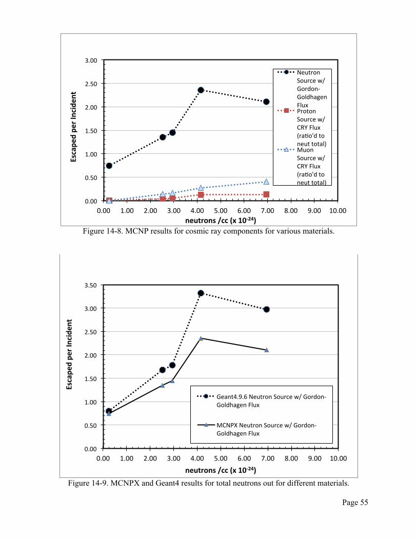
Page 55
Figure 14-8. MCNP results for cosmic ray components for various materials.
Figure 14-9. MCNPX and Geant4 results for total neutrons out for different materials.
0.00
0.50
1.00
1.50
2.00
2.50
3.00
0.00 1.00 2.00 3.00 4.00 5.00 6.00 7.00 8.00 9.00 10.00
Escape
d pe
r Inciden
t
neutrons /cc (x 10-‐24)
Neutron Source w/ Gordon-‐Goldhagen Flux Proton Source w/ CRY Flux (rabo'd to neut total) Muon Source w/ CRY Flux (rabo'd to neut total)
0.00
0.50
1.00
1.50
2.00
2.50
3.00
3.50
0.00 1.00 2.00 3.00 4.00 5.00 6.00 7.00 8.00 9.00 10.00
Escape
d pe
r Inciden
t
neutrons /cc (x 10-‐24)
Geant4.9.6 Neutron Source w/ Gordon-‐Goldhagen Flux
MCNPX Neutron Source w/ Gordon-‐Goldhagen Flux
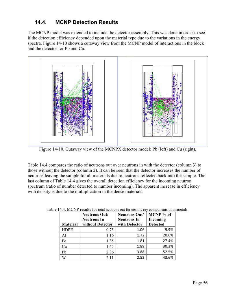
Page 56
14.4. MCNP Detection Results
The MCNP model was extended to include the detector assembly. This was done in order to see if the detection efficiency depended upon the material type due to the variations in the energy spectra. Figure 14-10 shows a cutaway view from the MCNP model of interactions in the block and the detector for Pb and Cu.
Figure 14-10. Cutaway view of the MCNPX detector model: Pb (left) and Cu (right).
Table 14.4 compares the ratio of neutrons out over neutrons in with the detector (column 3) to those without the detector (column 2). It can be seen that the detector increases the number of neutrons leaving the sample for all materials due to neutrons reflected back into the sample. The last column of Table 14.4 gives the overall detection efficiency for the incoming neutron spectrum (ratio of number detected to number incoming). The apparent increase in efficiency with density is due to the multiplication in the dense materials.
Table 14.4. MCNP results for total neutrons out for cosmic ray components on materials.
Material
Neutrons Out/ Neutrons In without Detector
Neutrons Out/ Neutrons In with Detector
MCNP % of Incoming Detected
HDPE 0.75 1.06 9.9% Al 1.16 1.72 20.6% Fe 1.35 1.81 27.4% Cu 1.45 1.89 30.3% Pb 2.36 3.88 52.5% W 2.11 2.53 43.6%
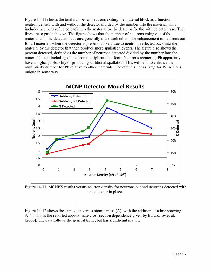
Page 57
Figure 14-11 shows the total number of neutrons exiting the material block as a function of neutron density with and without the detector divided by the number into the material. This includes neutrons reflected back into the material by the detector for the with detector case. The lines are to guide the eye. The figure shows that the number of neutrons going out of the material, and the detected neutrons, generally track each other. The enhancement of neutrons out for all materials when the detector is present is likely due to neutrons reflected back into the material by the detector that then produce more spallation events. The figure also shows the percent detected, defined as the number of neutrons detected divided by the number into the material block, including all neutron multiplication effects. Neutrons reentering Pb apparently have a higher probability of producing additional spallation. This will tend to enhance the multiplicity number for Pb relative to other materials. The effect is not as large for W, so Pb is unique in some way.
Figure 14-11. MCNPX results versus neutron density for neutrons out and neutrons detected with
the detector in place. Figure 14-12 shows the same data versus atomic mass (A), with the addition of a line showing A0.73. This is the reported approximate cross section dependence given by Barabanov et al. [2006]. The data follows the general trend, but has significant scatter.
0%
10%
20%
30%
40%
50%
60%
0
0.5
1
1.5
2
2.5
3
3.5
4
4.5
5
0 1 2 3 4 5 6 7 8
% Detected
Neu
rons Out/In
Neutron Density (n/cc * 1024)
MCNP Detector Model Results Out/In w/ Detector
Out/In w/out Detector % Detected
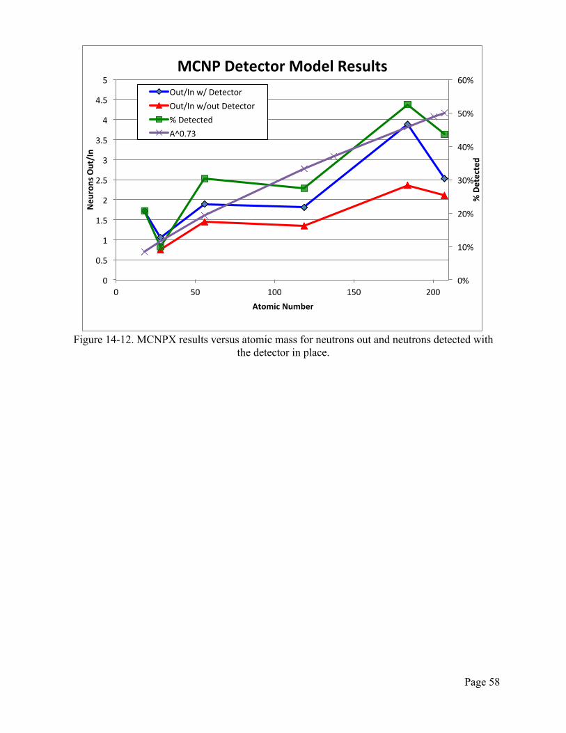
Page 58
Figure 14-12. MCNPX results versus atomic mass for neutrons out and neutrons detected with
the detector in place.
0%
10%
20%
30%
40%
50%
60%
0
0.5
1
1.5
2
2.5
3
3.5
4
4.5
5
0 50 100 150 200
% Detected
Neu
rons Out/In
Atomic Number
MCNP Detector Model Results Out/In w/ Detector
Out/In w/out Detector % Detected A^0.73
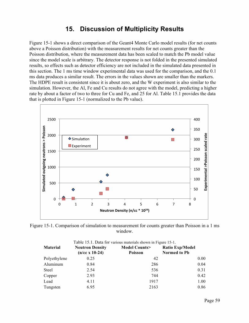
Page 59
15. Discussion of Multiplicity Results
Figure 15-1 shows a direct comparison of the Geant4 Monte Carlo model results (for net counts above a Poisson distribution) with the measurement results for net counts greater than the Poisson distribution, where the measurement data has been scaled to match the Pb model value since the model scale is arbitrary. The detector response is not folded in the presented simulated results, so effects such as detector efficiency are not included in the simulated data presented in this section. The 1 ms time window experimental data was used for the comparison, and the 0.1 ms data produces a similar result. The errors in the values shown are smaller than the markers. The HDPE result is consistent since it is about zero, and the W experiment is also similar to the simulation. However, the Al, Fe and Cu results do not agree with the model, predicting a higher rate by about a factor of two to three for Cu and Fe, and 25 for Al. Table 15.1 provides the data that is plotted in Figure 15-1 (normalized to the Pb value).
Figure 15-1. Comparison of simulation to measurement for counts greater than Poisson in a 1 ms
window.
Table 15.1. Data for various materials shown in Figure 15-1. Material Neutron Density
(n/cc x 10-24) Model Counts>
Poisson Ratio Exp/Model Normed to Pb
Polyethylene 0.25 42 0.00 Aluminum 0.84 286 0.04 Steel 2.54 536 0.31 Copper 2.93 744 0.42 Lead 4.11 1917 1.00 Tungsten 6.95 2163 0.86
0
50
100
150
200
250
300
350
400
0
500
1000
1500
2000
2500
0 1 2 3 4 5 6 7 8 Expe
rimen
tal >Po
isson scaled
rate
Simulated
outgoing ne
utrons > Poisson
Neutron Density (n/cc * 1024)
Simulabon
Experiment
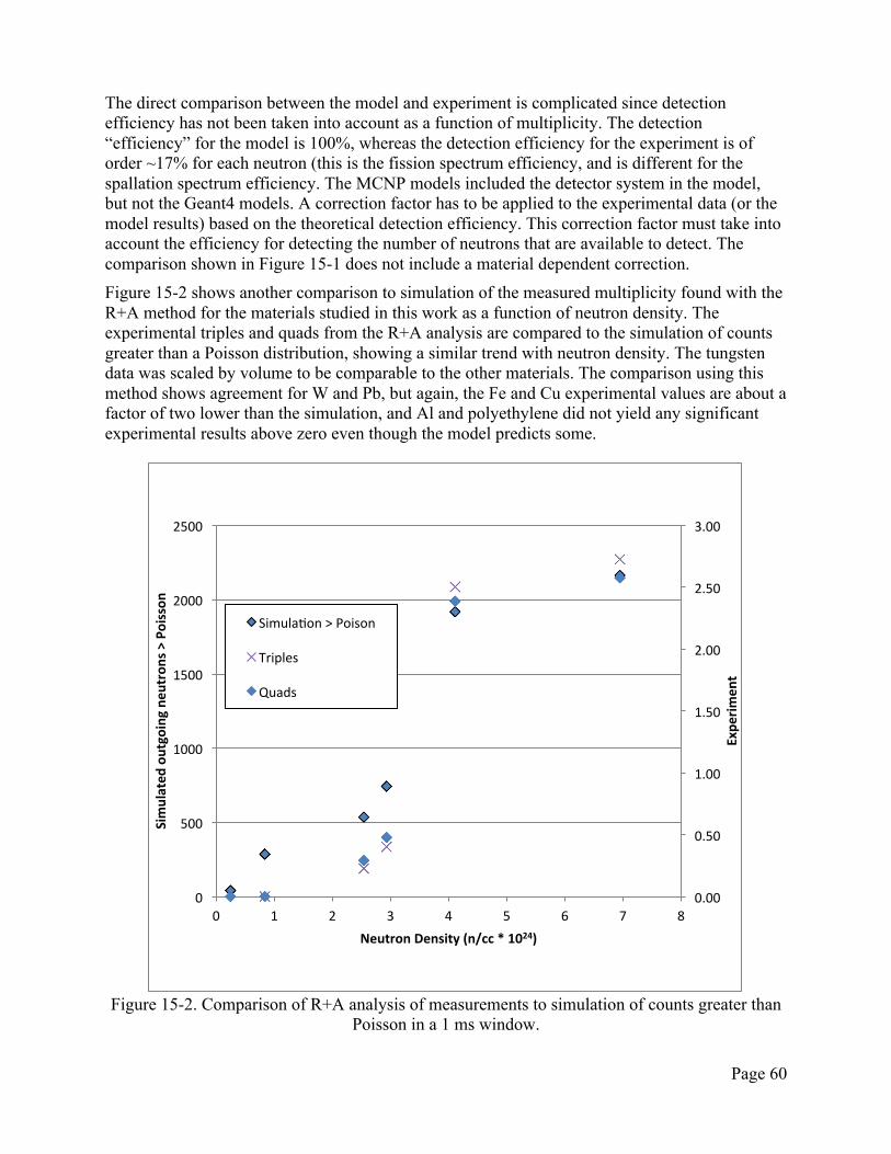
Page 60
The direct comparison between the model and experiment is complicated since detection efficiency has not been taken into account as a function of multiplicity. The detection “efficiency” for the model is 100%, whereas the detection efficiency for the experiment is of order ~17% for each neutron (this is the fission spectrum efficiency, and is different for the spallation spectrum efficiency. The MCNP models included the detector system in the model, but not the Geant4 models. A correction factor has to be applied to the experimental data (or the model results) based on the theoretical detection efficiency. This correction factor must take into account the efficiency for detecting the number of neutrons that are available to detect. The comparison shown in Figure 15-1 does not include a material dependent correction. Figure 15-2 shows another comparison to simulation of the measured multiplicity found with the R+A method for the materials studied in this work as a function of neutron density. The experimental triples and quads from the R+A analysis are compared to the simulation of counts greater than a Poisson distribution, showing a similar trend with neutron density. The tungsten data was scaled by volume to be comparable to the other materials. The comparison using this method shows agreement for W and Pb, but again, the Fe and Cu experimental values are about a factor of two lower than the simulation, and Al and polyethylene did not yield any significant experimental results above zero even though the model predicts some.
Figure 15-2. Comparison of R+A analysis of measurements to simulation of counts greater than
Poisson in a 1 ms window.
0.00
0.50
1.00
1.50
2.00
2.50
3.00
0
500
1000
1500
2000
2500
0 1 2 3 4 5 6 7 8
Expe
rimen
t
Simulated
outgoing ne
utrons > Poisson
Neutron Density (n/cc * 1024)
Simulabon > Poison
Triples
Quads
Page 61
These results for multiplicity indicate that there is a discrepancy between the model results and the measurements for the lighter materials. Since the measurements were in a controlled geometry and the data rates, and resulting dead time, were small, there is no obvious problem with the measurements, except that the tungsten measurement had to scaled to match the geometry of the rest of the studied materials. With regard to the model, there are several possible explanations: the incoming neutron spectrum might be different than assumed, the cross-section libraries might be wrong between materials, or simplification of the model might cause the observed differences.
The origin of this discrepancy requires further investigation: is there a problem with the measurements or with the models? If this disagreement is correct, the model over predicts the interaction rate for lower density materials (Al, Fe, and Cu), and thus the effectiveness of iron and copper shielding on the incoming neutrons could be substantially smaller than currently assumed. There are differences in the neutron spectra that come from spallation in the various materials, as discussed, but these spectra are similar in that much of the neutron flux is below one MeV where the detection efficiency is high. The development of targets for spallation neutron source facilities has developed a good basis for heavy target production rates used in the simulations; however, lighter materials like aluminum, iron and copper may not have validated cross sections for the cosmic energies studied here. Experimental measurements of neutron energy spectra exiting thick targets of these materials should be made with incident spectra similar to that from cosmic rays.
Page 62
16. Conclusions
This paper has reported on multiplicity measurements for a range of materials and compared them to Monte-Carlo modeled results based on the Geant4 and MCNPX simulation codes. Measurements of neutron multiplicity were performed using a neutron coincidence counter with a list mode data acquisition system that recorded the time of each detected neutron. Post analysis was performed to extract the detected multiplicity. Measurements were made on polyethylene, aluminum, iron, copper, lead and tungsten. The evaluation reported here was undertaken to study the fidelity of Monte Carlo models to simulate spallation neutron yields from different shielding materials induced by cosmic-rays. This was motivated by the large difference between shield model results from two different simulations. Geant4 predicted a greater degree of shielding by the iron shipping shield than the SHIELD code by a factor of ~2.5. This difference is what motivated the current study to see how well a model could predict experimental results. The result of this study is that the relative multiplicity per event extracted from the models are in agreement for dense materials, but disagree with the experimental findings by a factor of more than two for the lower density materials Al, Fe and Cu. The model over-predicts the effect of Fe shielding by about a factor of three, making the experimental results more consistent with the SHIELD code predictions. This might be an artifact of the way the neutron data was obtained, or it may represent limitations in the models for low-density materials. A number of experimental tests were made indicating that the experimental results are probably correct, which points to the model results as being the more likely problem. Two Monte Carlo approaches, Geant4 and MCNPX, were compared to each other to confirm the reproducibility of the experimental results with different independently developed codes. The last official release of MCNPX (version 2.70) did not provide a tally option for tabulating the multiplicities of the target materials studied, so an alternative simulation scenario was devised for this inter-code comparison. Several simulation runs involving mono-energetic neutrons in the range of interest for cosmic ray studies were performed and the result of the inter-code comparison is an agreement by better than ~30% in the total neutron yield.
The scope of this work was not to reproduce accurately the experimental set-up, but simply to evaluate the models’ behavior when switching between different shielding materials. This result shows that the Geant4 Monte Carlo model results follow the correct trend as determined by experiment for total neutron yield and multiplicity. The predicted multiplicity as a function of target material increased with material density, with an approximately linear relationship. This indicates that Geant4 can provide adequate predictions for the spallation effects of cosmic ray neutrons, with the caveat that spallation rates for lower density materials are over-predicted by the models. The MCNP models showed that only a small percentage of the incident cosmic neutron flux is not scattered in a cubic foot of target material, being 9% for HDPE and decreasing to 0.04% for tungsten. The MCNP models also looked at the contributions from cosmic proton and muon secondaries on the Earth’s surface. It was predicted that these two components could contribute 12% to the outgoing neutrons for iron, increasing up to 20% for tungsten.
These theoretical tools must be used with care to correctly simulate shielding techniques for the next generation of low-background experiments and to estimate background rates. Unless
Page 63
benchmark measurements are made to validate Monte Carlo modeling for each application, there use is limited to shielding comparison studies, not as a predictor of absolute shielding efficiency. Future measurements should be performed of neutron spectra exiting large quantities of materials, especially the lower density materials where there remains a large uncertainty in the ability of the models to correctly predict the effects of such materials.
Page 64
17. Acknowledgements
This work was supported by the United States Department of Energy Office of Science Office of Nuclear Physics. Pacific Northwest National Laboratory is operated for the United States Department of Energy under contract DE-AC05-76RLO 1830.
Page 65
18. References
Aalseth CE, et al. (MAJORANA collaboration). 2009. “The MAJORANA DEMONSTRATOR: An R&D project towards a tonne-scale germanium neutrinoless double-beta decay search.” The American Institute of Physics, Conf. Proc. 1182 pp 88-91.
Aguayo Navarrete E, RT Kouzes, AS Ankney, JL Orrell, TJ Berguson, and MD Troy. 2011. “Cosmic Ray Interactions in Shielding Materials.” PNNL-20693, Pacific Northwest National Laboratory, Richland, WA Aguayo E, JE Fast, RT Kouzes, JL Orrell. 2112a. “The µ-Witness detector: A ruggedized, portable, flux meter for cosmogenic activation monitoring.” Transactions on Nuclear Science. Aguayo E, RT Kouzes, JL Orrell, DJ Reid, JE Fast. 2012b. “Optimization of the Transport Shield for Neutrinoless Double-beta-decay Enriched Germanium.” PNNL Technical Report PNNL-21302.
Agostinelli S, et al. 2003. “Geant4-a Simulation Toolkit.” Nuclear Instruments & Methods in Physics Research Section a-Accelerators Spectrometers Detectors and Associated Equipment 506(3):250-303. 10.1016/s0168-9002(03)01368-8. Allkofer OC, K Carstensen, WD Dau, H Jokisch. 1975. “The Absolute Cosmic Ray Flux at Sea Level.” J Phys. G: Nucl. Phys. 1, No. 6. L51-L52. Armstrong TW, KC Chandler, J Barish. 1973. Journal of Geophysical Research 78 pp. 2715-2726. Barabanov, I, S Belogurov, L Bezrukov, A Denisov, V Kornoukhov, and N Sobolevsky. 2006. "Cosmogenic Activation of Germanium and Its Reduction for Low Background Experiments." Nuclear Instruments and Methods in Physics Research Section B: Beam Interactions with Materials and Atoms 251(1):115-20. Crane TW and MP Baker. 1991. Chapter 13 in “Neutron Detectors,” in Passive Nondestructive Assay of Nuclear Materials, edited by T. D. Reilly, N. Ensslin, and H. A. Smith, US Nuclear Regulatory Commission NUREG/CR-5550.
Ensslin N, WC Harker, MS Krick, DG Langner, MM Pickrell and JE Stewart. 1998. “Application Guide to Neutron Multiplicity Counting.” Los Alamos National Laboratory Technical Report LA-13422-M.
Grieder PKF. 2001. “Cosmic Rays at Earth.” Elsevier, Amsterdam.
IS, JR Hook, IA Jenkins, KE Turver. 1974. “Momentum Spectra Of Nuclear Active Particles In Cosmic-Radiation At Sea-Level .1. Experimental-Data.” Journal Of Physics A-Mathematical And General 7, Issue 6, pp. 741-764 GE Reuter Stokes Measurements Solutions (Twinsburg, OH). Gordon MS, P Goldhagen, KP Rodbell, TH Zabel, HHK Tang, JM Clem, and P Bailey. 2004. “Measurement of the Flux and Energy Spectrum of Cosmic ray Induced Neutrons on the Ground.” IEEE Transactions On Nuclear Science, Vol. 51, No. 6; and private communication of data from P Goldhagen.
Page 66
Greisen KI. 1942. “The Intensities Of The Hard And Soft Components Of Cosmic Functions Of Altitude And Zenith Angle.” Phys. Rev. 61, pp. 212-221. Hagmann C, D Lange, D Wright. 2008. "Cosmic ray Shower Library (CRY)." Technical Manual, 5 pages. Lawrence Livermore National Laboratory, Livermore, CA. http://nuclear.llnl.gov/simulation/cry.pdf.
Geant4. 2011. The Geant4 Collaboration. Physics Lists - Use Cases. Accessed on July 22, 2011 at http://geant4.org/geant4/support/physicsLists/referencePL/useCases.shtml (last updated July 9, 2011). Hess WN, HW Patterson, R Wallace, EL Chupp. 1959. "Cosmic ray Neutron Energy Spectrum." Physical Review 116 pp 445-57. Kouzes RT, JH Ely, A Seifert, ER Siciliano, DR Weier, LK Windsor. 2008. “Cosmic-Ray-Induced Ship-Effect Neutron Measurements And Implications For Cargo Scanning At Borders.” Nuclear Instruments And Methods In Physics Research A 587 Pp. 89-100.
MCNP. 2003. X-5 Monte Carlo Team, MCNP - A General Purpose Monte Carlo N-Particle Transport Code, Version 5, Los Alamos National Laboratory Report LA-UR-03-1987, updated 2005. Pelowitz DB (ed.). 2011. “MCNPX User’s Manual”, Version 2.7.0. Los Alamos National Laboratory Report LA-CP-11-00438. Prael RE and H Lichtenstein. 1989. “Users Guide to LCS: The LAHET Code System.” Los Alamos National Laboratory Report LA-UR-89-3014. Prael RE. 1994. “A Review of the Physics Models in the LAHET Code.” Los Alamos National Laboratory Report LA-UR-94-1817. Switzer T, RR Hansen, RT Kouzes, RJ Arthur, WK Pitts. 2003. “Neutron Detection Authentication Case Study.” Technical Report PNNL-14222 Ziegler JF. 1998. "Terrestrial Cosmic Ray Intensites." IBM Journal of Research and Development 42(1):117.