shocks and policy responses in the open economyuctpa36/ch6feb03.pdf · chapter 6 shocks and policy...

CHAPTER 6

Shocksand policy responses in theopen economy

[This is a draft chapter of a new book - Carlin & Soskice (200x)1].In this chapter, the open economy model developed in Chapters 4 and 5 is put to work to ex-

amine government policy instruments and to analyze shocks that may disturb the economy. Theterm ‘shocks’ is used to describe a disturbance to the economy that was unanticipated. Firms andhouseholds are likely to be forward-looking and, at least to some extent, are able to incorporateanticipated changes in their economic environment into their behaviour. It is the different kinds ofunanticipated changes in the economic environment on which we focus in this chapter. We use themodel to analyse

� aggregatedemand shocks,� supply shocks and� external shocks.

In each case, it isnecessary to diagnose the implicationsof thedisturbance for theprivatesectorand for policy-makers — does it shift the��-curve, is it a shift along the��-curve, does it shiftthe�� -curve or the��-curve? In order to assess the likely response of the private sector to theshock and to examine the appropriate policy response of the authorities, a diagnosis of the type ofshock has to be made. Some shocks are relatively simple to analyze in the sense that they have animpact on only oneof thethreerelationships in themodel. Othersaremorecomplex — for example,shifting more than one relationship.

The importance of the correct diagnosis of the type of shock is demonstrated by the experienceof the advanced countries in the 1970s. In 1973 and again in 1979, the world price of oil increasedsharply. The consequence of the first oil shock was a fall in aggregate demand in the oil-importingOECD countries. Many countries adopted policies in response to thefirst oil shock based on the in-terpretation of it asan aggregatedemand shock — onethat shifted theaggregatedemand curveto theleft. Yet the attempt to offset the impact of the shock on employment through fiscal expansion wasaccompanied by rapid deterioration in the tradebalance and rising in�ation. A number of Europeancountriesexperienced in�ation ratesrising well into doubledigitsat a timeof rising unemployment.The second oil shock in 1979 was met by quite a different policy response. By then it was clearerthat the rise in the price of oil was an external supply shock, which had the effect of shifting the��-, �� - and��-curves in an adversedirection.

Another example is the slowdown in productivity growth in the advanced countries from theearly 1970s. Although the languageof ‘shocks’ fits the case of a change in the productivity growthtrend less well, it is still a useful way of conveying the idea of an unanticipated change in trend.Usually it is only with hindsight that it ispossible to identify cyclical changes in aggregatedemand,commodity prices or productivity growth from longer lasting movements. An interesting questionin the early 21st century is whether the rise in productivity growth in the United States from themid 1990s signals a new trend of higher productivity growth — due for example to the widespreadintroduction of new information technologies— or simply an usually long cyclical upswing.

Theanalysisof different kindsof shocks, privatesector responsesand theefficacy of governmentpolicy measures also provides some of the tools that are needed in analyzing how a currency union

1 c�Wendy Carlin & David Soskice (2003). Wearevery grateful to Andrew Glyn, Georg von Graevenitz, Massimodi Matteo, NicholasRau and William Wachtmeister for their help and advicebut weareresponsible for all errors.

1

2 6. SHOCKS AND POLICY RESPONSES IN THE OPEN ECONOMY

operatesand theadvantagesand disadvantagesof membership. Chapter (Interdependent Economies)on themacroeconomicsof European Monetary Union explores this further.

This chapter begins with an introductory section that looks at fiscal, monetary and supply-sidepolicy in theopen economy. This ties together theMundell–Fleming analysis (from Chapter 4) withthemedium- and long-run analysis in Chapter 5. Thisisfollowed by an examination of four differentkinds of shocks: domestic aggregatedemand shocks, domestic supply shocks, foreign tradeshocks,and external supply shocks. In eachcase, weask what theimplication of such ashock isfor theshort-run, themedium-run and thelong-run equilibrium. Thishelpsusto analysewhat would happen aftereach kind of shock if the government did not react to it at all. We can then ask whether there areappropriate tools available to the government with which to offset such a shock or to mitigate itseffects on theeconomy.

There is then a summary section that draws together conclusions for the usefulness of the dif-ferent policy instruments. The chapter ends with a short section that examines the implications of�uctuationsin aggregatedemand andof supply-sidepolicy measuresfor thebehaviour of real wages.

1. Fiscal, monetary, exchange rateand supply-sidepolicies

The open economy model is very useful for analyzing the impact on the economy of policychanges at home and abroad as well as the impact of shifts in private sector behaviour. The keycomponentsof themodel set out in Chapter 5 are:

� the��-curve. This shows thecombinations of the real exchange rate� and level of output at which thegoodsmarket is in equilibrium and thereal interest rate isequal to theworldreal interest rate.

� the�� -curve. This is defined as the combinations of the real exchange rate and outputat which thewage-setting real wage is equal to theprice-setting real wage. At any point onthe��-curve, in�ation is constant.

� the �� -curve. This shows the combinations of the real exchange rate � and the level ofoutput at which trade isbalanced: � �.

Timing assumptions. This is an appropriate point at which to spell out the assumptions thatare being made about the speed of adjustment of different macroeconomic variables in the openeconomy.

: The short run. In the short run, the goods market equilibrium is established and arbitragein financial markets ensures that the home real interest rate is equal to the world real in-terest rate. In the short run, we observe changes in the nominal interest rate, the nominalexchange rate, output and employment.2 The end of the short-run adjustment is marked bytheattainment of theshort-run equilibrium on the��-curve. In theshort run, it isassumedthat wageand price-setters do not changewages or prices.

: The medium run. The medium run begins when wage and price-setters start to respond totwo things:� to any change in the level of activity (output, employment) in the economy that has

occured in the short run and� to any change in thereal wagethat hasbeen brought about by achange in thenominal

(and hence the real) exchange rate in theshort run.: Wage-setting isassumed to happen periodically and price-settersareassumed to adjust their

prices rapidly in the wake of wage changes. This means that the actual real wage in theeconomy is always equal to the price-setting real wage.3 The end of the medium run is

2By virtue of any change in the exchange rate, the consumer price index changes. Although this will in�uence theshort-run equilibrium in themoney market, thiseffect isnormally ignored.

3Thisisobviously asimplification — if price-setting issluggish in thewakeof cost increases, then thereal wagewillliebetween thewage-setting real wageand theprice-setting real wage (i.e. between the��-curveand the��-curve).

1. FISCAL, MONETARY, EXCHANGE RATE AND SUPPLY-SIDE POLICIES 3

marked by theattainment of themedium-run equilibrium with theeconomy at the intersec-tion of the��-curveand the��-curve, and hencewith constant in�ation.

: The long run. In the long run, the presence of a current account surplus or deficit mayproduceshifts in the��-curve(asconsumersreact to thechangesin wealth implied, or thegovernment adjustsfiscal policy in response to market or political pressures). Thepresenceof apersistent surplusor deficit may lead to achangein theway exchangerateexpectationsare formed, with the consequence that there is constant in�ation only at the intersection ofthe�� and �� curves as discussed in Chapter 5. This in turn may lead the governmentto adjust fiscal policy to shift theeconomy to the long-run equilibrium.

In thissection, weconcentrateon threekey results from the open economy model:

� a change in fiscal policy shifts the aggregate demand curve, which implies there is a newmedium-run equilibrium for the economy at a different level of output and real exchangerate. In the absence of government intervention, the economy moves from the new short-run equilibrium to the new constant-in�ation rate of unemployment. Since the short-runequilibrium is different under fixed and �exible exchange rates, the adjustment path to thenew medium-run equilibrium differs under fixed and �exible exchange rates. In particular,the impact on in�ation — whether there is a temporary rise or a temporary fall in in�ation— depends on theexchange rate regime.

� a change in monetary policy under �exible exchange rates or a change in the exchangerate peg in a ‘fixed’ exchange rate system is a shift along the aggregate demand curveand therefore does not lead to a new medium-run equilibrium. The levels of output andunemployment change only in the short run. A temporary rise in in�ation in the case of adevaluation/expansionary monetary policy or a temporary fall in in�ation in the case of arevaluation/contractionary monetary policy leadstheeconomy back to theoriginal mediumrun equilibrium.

� a change in supply-side policy is a shift in the�� -curve (under both fixed and �exibleexchange rates). This changes both themedium and the long-run equilibrium.

Wearenot concernedherewithwhy thegovernment might want tousefiscal or monetary/exchangerate policy or supply-side policy — we come to that when we look at the different kinds of shocksthat may affect theeconomy. For now, theaim issimply to pin down theeffectsof different policies.This is easiest to understand if we begin in full equilibrium at the intersection of the��-, �� - and�� -curves.

1.1. Fiscal policy. We focus on the implications for aggregate demand of a change in fiscalpolicy: we examine the supply-side aspects of some kinds of fiscal policy later on when we lookat supply-side policy. Suppose the economy is at point � at full equilibrium in Figure 6.1. Thegovernment undertakesan expansionary fiscal policy. Theaggregatedemand curvethen shifts to theright. (A fiscal contraction will producean exactly symmetrical set of results.)New medium-run equilibrium. A fiscal expansion implies a rightward shift of the��-curve. Thisleads to anew medium-run equilibrium at point �. At thenew medium-run equilibrium,

� output is higher and unemployment lower,� � is lower (i.e. a real appreciation), and the real wage ishigher,� there isa trade deficit, and� in�ation isconstant.

This example was discussed at the beginning of Chapter 5, where we used the labour marketdiagram to discuss the implicationsof afiscal expansion. Theadjustment path from� to� dependson theexchange rate regime.Under fixed exchange rates. As we saw in Chapter 5, under fixed exchange rates, output in theeconomy expandswith thereal exchangerateconstant. In theMundell–Flemingmodel expansionaryfiscal policy has the full multiplier effect on output because in the new short-run equilibrium, theinterest rate remains unchanged at the world rate. In Fig. 6.1, this is the move from � to �. But


��

��

��

��

��

��

��

��

�

�

��

��

��

�

�

�

FIGURE 1. Fiscal policy shifts the AD-curve: New medium-run equilibr ium atB and compar ison with Mundell-Fleming predictions

in the medium run, after output and employment in the economy have expanded, wages and priceswill begin to respond. At aposition above the�� -curve (seeFig. 6.1), theexisting real wage liesbelow the wage-setting real wage at the new higher level of activity (see Fig. 5.2). The reason isthat the �-curve is upward-sloping: as employment rises, so does the real wage that wage-setterscan expect when money wages are set. As a consequence, at the next occasion on which wages areset, wages rise relative to expected in�ation. From the pricing equation (� � �

�� , we know

that when money wages rise, prices will be put up by home firms in proportion to the labour costincrease in order to keep themark-up, �, constant. Two things follow from this.

: First, from thedefinition of theconsumer priceindex (�� ), it followsthat consumer prices rise in the wake of the home price rise. However, the consumer priceindex will not rise by as much as does the price level of home-produced output becausenothing has happened to the rate of in�ation for imported goods. This implies that the realwage, � ��, has increased.

: Second, becausehomein�ation hasrisen and nothing hashappened to world in�ation, pricecompetitiveness,

��

�

�has fallen. Another way of looking at this is that, in terms of

the goods that the home economy exports, imports have become cheaper, i.e. the real costof importshas declined.

Theeconomy thereforemoves in asouth-westerly direction down the��-curve. This is themirror-image of the north-westerly movement in the labour market diagram in Fig. 5.2. The homeeconomy experiences a temporary rise in in�ation relative to world in�ation. Once the economy isat point �, real wages, the real exchange rate and in�ation are constant. An example is provided inthe appendix to this chapter of how in�ation changes as the economy moves from one medium-runequilibrium with constant in�ation to another one — for example, following an expansionary fiscalpolicy.Under �exible exchange rates. In the Mundell–Fleming model, the increase in output stimulated bya fiscal expansion is wiped out in the short run by the exchange rate appreciation induced by the


fact that the home nominal interest rate is temporarily higher than the world rate. In the mediumrun, however, there is higher output at the new equilibrium. As we saw in Chapter 5, the initialnominal exchangerateappreciation to point � (theMundell–Fleming short-run equilibrium) in Fig.6.1 implies that price competitiveness has fallen and real wages have risen. Real wages have risenbecausethenominal appreciation cutstheprice(in domestic currency terms) of imported final goods

in theconsumption bundle (i.e. � ��

�). In themedium run, wagesetterswill react to

this. With real wages at � above the level associated with wage-setting equilibrium, money wageswill fall relativeto theexpected pricelevel (refer back to Fig. 5.2). Sincethisreduceslabour costsforfirms, home prices are reduced by price-setters in line with the fall in nominal wages. Nothing hashappened to world in�ation so the consumer price index falls by less than the fall in the price levelof home goods. The consequence is that real wages do fall. Since home in�ation has fallen belowworld in�ation, price competitiveness rises (the real exchange rate depreciates). The improvementin competitivenessboostsnet exportsand theeconomy moves in anorth-easterly direction along the��-curve toward the new medium run equilibrium at � (this mirrors the south-easterly movefrom point � in Fig. 5.2). The home economy experiences a temporary fall in in�ation relative toworld in�ation.Summing up. Following an expansionary fiscal policy,

� under fixed exchange rates, adjustment to the new medium-run equilibrium is via risingoutput and a temporary increase in in�ation (relative to world in�ation), which weakenscompetitiveness and dampens theexpansion.

� under �exible rates, adjustment is via an initial exchange rate appreciation that offsets theeffect of the expansionary fiscal policy on output. This is followed by a temporary fall inin�ation (relative to world in�ation), which boosts competitiveness and raisesoutput.

1.2. Monetary and exchange rate policy. In a �exible exchange rate economy with perfectcapital mobility, monetary policy worksthrough itseffectson thenominal exchangerate. Aswesawin Chapter 4, achangein monetary policy changesthehomeinterest raterelativeto theworld interestrate and this leads to a change in the nominal exchange rate. In the new short-run equilibrium, thenominal interest rate isoncemoreequal to theworld interest rateand there isadifferent level of thenominal exchange rate.

Wecan recall from Chapter 4 that in afixed exchange rate regimemonetary policy is ineffectualeven in the short run. The requirement to keep the nominal exchange rate fixed means that anychange in domestic monetary policy is wiped out by offsetting changes in the monetary basebeforeit gets off the ground. Therefore the analogue to monetary policy in a fixed exchange rate regime isthe possibility that the exchange rate peg can be changed. A devaluation mimics an expansionarymonetary policy: the rightward shift in the �� raises the domestic interest rate and induces acapital in�ow, which shifts the �� to the right. Similarly, a revaluation mimics a contractionarymonetary policy by inducing acapital out�ow.

Let usnow look moreclosely at theshort and medium run consequencesof changesin monetarypolicy (under �exible exchange rates) and a one-off change in the exchange rate peg under fixedexchange rates. Under �exible exchange rates, monetary policy is very effective in raising outputin the Mundell–Fleming model. Monetary expansion has a strong impact because of the boost toaggregatedemand dueto theexchangeratedepreciation induced by thetemporary fall in theinterestrate below the world rate. If we turn to the medium run, then we know that a change in monetarypolicy under �exibleexchangeratescannot shift themedium-run equilibrium: in Figure6.2 the��-curve and the�� -curve remain fixed so the medium run equilibrium remains at point �. Exactlythesameanalysisapplies in thecase in which there isadiscretechange in theexchangerateunder a‘fixed’ ratesystem (from �� to �� — seeFig. 6.2).

Following a loosening of domestic monetary policy or a nominal devaluation, net exports andoutput expand to �: the short-run Mundell–Fleming equilibrium is at point �. However, in themedium run, with the economy at point �, wemust consider the implications for the supply side of


��

��

��

��

��

��

��-curve

�

�

�

��

��

� ��

in�ationary pressure due

in�ationary pressure dueto � �

to depreciation (�� to ��)

�

depreciationor

devaluation

FIGURE 2. Monetary/exchange rate policy is a shift along the AD-curve:medium run equilibr ium remainsunchanged at A

the economy. The real depreciation of the exchange rate implies a lower real wage. This is becausetherise in thepriceof imports, i.e. �� due to theexchange ratedepreciation from �� to ��,impliesadeterioration in thetermsof tradefor thehomeeconomy. Sincethepriceof exportshasnotchanged, a rise in the price of imports turns the terms of tradeagainst the home economy. This cutsreal wagesbecauseworkersconsumeboth imported and home-produced goods. Thehigher priceofimports feedsdirectly into theconsumer price index and cuts the real wage.

In the medium run, wage-setters will react to the rise in employment and the fall in the realwage. Since output has increased in the short run from � to �, there are two sources of pressurepushing money wages up: the fall in unemployment means a higher wage-setting real wage and thedepreciation means that the actual real wage has fallen. The result will be a rise in money wagesrelative to expected prices followed by an increase in the prices of home produced goods relative toworld prices. After the initial depreciation, thenominal exchangerateremainsfixed so that thereareno further changes in import prices. As a consequence, the consumer price index rises by less thanmoney wages: real wagesriseand pricecompetitiveness falls. Thispattern is familiar: theeconomyis above the�� -curve and as we have seen before, this results in a temporary burst of in�ation(above world in�ation) until the real wage has risen to a level equal to the wage-setting real wage.The rise in homerelative to world in�ation eatsaway at the initial rise in competitivenessdue to thedepreciation/devaluation and theeconomy moves back to point � (seeFig. 6.2).Summing up. Following an expansionary monetary policy or adevaluation, output and employmentexpand due to the effect of the rise in competitiveness on net exports. But this is only a temporaryeffect: since the devaluation has its effect by raising the real cost of imports, once wages and pricesrespond to this, therewill beabout of domestic wageand pricein�ation in excessof world in�ation.The higher in�ation will reverse the boost to competitiveness and the cut in real wages and theeconomy will return to itsoriginal position.

1.3. Supply-sidepolicy. To analyzesupply-sidepolicies, wehave to focusour attention on the�� -curve. Supply-sidepoliciesarethosethat shift the��-curve— either by shifting thewage-setting curve � �� or by shifting the price-setting curve ��. In Chapter 2 the determinantsof the wage and price setting curves were introduced. Here we apply that discussion to the openeconomy.

It is useful to separate out the factors that shift the �-curve from those that shift the��-curve. Wecan recall from Chapter 2 that when we introducetaxesinto thesupply-sideof themodel,


it is necessary to be careful in defining both the money wage and the price level. We stick to theprinciple that the real wage shown on the vertical axis of the � � ��-diagram is the real wagerelevant to wage-setters. This isthereal consumption wagedefined asthe“ takehome” wagede�atedby theconsumer price index:

� �

��

wagenet of incometax and social security

consumer price index including VAT(real consumption wage)

Policies that shift thewage-setting curve. Thewagesetting curveshowsthereal takehomewageat each level of employment that workers believe they have negotiated. As discussed in Chapter 2,thewagesetting curve liesabove thecompetitive labour supply curveeither becauseof thepresenceof unions or because of efficiency wage considerations. At each level of employment, wage-settersset themoney wageto securethisreal wage, assuming that aspecific price level will prevail over thecourseof the wagecontract.

� �� (wageequation)

Thewage-setting curve is therefore:

��

��

� �� (wagesetting real wage)

Any policy that affects the wage-setting decision will shift the �-curve. Policies discussed inChapter 2 include changes in the worker’s outside option such as changes in unemployment ben-efit, labour legislation, or the negotiation by the government of a wages accord with unions andemployers’ associations.

The �-curveshiftsdown

� if thereisafall in unemployment benefits(or moreprecisely in thereplacement ratio, whichis the ratio of benefits to theaverage wage),

� if unionsaregiven less legal protection,� if unions agree to exercise bargaining restraint — in the context, for example, of a wages

accord.

Policies that shift the price-setting curve for a given real exchange rate. We turn now to the policiesthat shift the��-curve. The price-setting curve shows the outcome for real consumption wagesof the decisions of the price-setters in the economy. Price-setters set their prices in order to securethe mark-up �, given the unit labour costs that they face. We saw in the closed economy that theprice-setting curvewill shift if there is achange in

� taxes— either direct taxesor indirect taxes� themark-up, due, for example, to achange in competitiveconditions� efficiency, such as achange in the level or the trend of labour productivity growth.

The ��-curve shifts up — showing that real take home wages in the economy consistentwith price-setting behaviour are higher — if there is a fall in the mark-up, in tax rates or a rise in‘efficiency’ . Wealso know that in theopen economy, theprice-setting curveshiftsasaconsequenceof changes in the real exchange rate. Since the�� -curve is drawn in real exchange rate—outputspace, although a change in � shifts the price-setting curve, it does not shift the��-curve. If theprice-setting curveshifts for any other reason, this implies ashift in the�� -curve.

Looking at each of these factors in turn, in the open economy, changes in the pressure of prod-uct market competition can arise from trade liberalization policies. A good example for Europeancountries is the reduction of tariff barriers to trade between members of the European EconomicCommunity, which began in 1957 with the Treaty of Rome. This was followed in the late 1980swith an initiative to removenon-tariff barriers to tradeso as to increase product market competitionin the internal market of the European Union. There is some evidence to suggest that monopoly


power has fallen in the EU following the so-called ‘1992’ Single Market measures.4 An increasein product market competition is likely not only to shift the ��-curve upwards but also shift the �-curve downwards. More pressure in the product market has the effect of dampening unionbargaining power. However, since both of these effects (an upward shift in the��-curve and adownward shift in the �-curve) shift the��-curve in the same direction, we simplify here byconsidering competition effects under ‘price-setting’ only.

Theanalysisof taxes isvery similar to that in theclosed economy. Theonly extra considerationis the tax treatment of exports and imports. Exports are exempt from value-added tax. The logicof this arrangement is that indirect taxes should be ‘destination-based’ in order that cross-countrydifferences in tax rates do not distort competition in the domestic market for final goods. Thisprinciple means that imports attract the VAT rate of the importing country. In the derivation of theprice-setting real wage that is set out in detail in theappendix to this chapter, these factorsare takeninto account.

The impact of a change in productivity (or in the rate of productivity growth in a dynamic con-text) on equilibrium employment dependson itseffectson thewage-setting and price-setting curves.If we abstract from productivity growth, and examine the impact of a policy that raises the level ofproductivity, themost obviouseffect is to shift theprice-setting real wageupward.5 Moreoutput perhead is available for real wages at each level of employment. Education and training policies mayhave theeffect of raising efficiency.

By recalling thederivation of the�� -curve (Chapter 5.1), it isclear that any policy that shiftsthe wage setting curve or shifts the ��-curve implies a shift in the ��-curve. A downwardshift in the �-curve implies ceteris paribus a rightward shift in the�� -curve. An upward shiftin the��-curve impliesceterisparibusarightward shift in the�� -curve. Wetakean exampleof asupply-sidepolicy that shifts the �-curveand another that shifts the��-curve.

Example: wage accord. In Figure 6.3, the �-curve shifts down. This could be for any of thereasons listed above. In this example, let us assume that it shifts because of the negotiation of awages accord by the government. The conclusion of an agreement through which unions agree toexercisebargaining restraint implies a rightward shift in the�� -curve, as explained above.

What are the implications for theeconomy? Consider an initial position of medium-run equilib-rium. Then shift the �-curve down. This re�ects the fact that at the existing employment level,wagesetterswill set a lower nominal wageto securethe lower expected real wage. At an unchangedlevel of thereal exchangerate(i.e. an unchanged real cost of imports) and with agiven profit margin,this implies that lower unemployment will be compatible with medium run equilibrium. At lowerunemployment the wage claims of wage setters will be boosted sufficiently so as to restore equalitybetween the price setting real wage (given � and �) and the wage setting real wage. The shift inthe wage-setting curve from � to � � implies a shift in the �� -curve to �� (see Figure6.3). To derive the new �� -curve from the �� diagram, note that at point � with � � �� at an employment level of �� This is re�ected in a point on �� of �� Wecan also see that � � � �� at employment level ��, i.e. at point �� This is re�ected in apointon�� of (��

Nothing happens in the short run because wages and prices are assumed to be given. The newmedium-run equilibrium for the economy is at point � with lower unemployment and higher pricecompetitiveness. The economy adjusts gradually from � to � in the following way: at � followingtheshift in the �-curve, theexisting real wage, ��, isabovethenew wage-setting real wageon the ��-curve. Money wages fall, home prices fall in line — but because nothing has happened to theprices of imported goods, theconsumer price index falls by less than does thepriceof homeoutput.

4See, for example, Allen, C., Gasiorek, M. and A. Smith. (1998) ‘The competition effects of the Single Market inEurope’ , Economic Policy, No. 27, pp. 441-486.

5Higher productivity may also have the effect of shifting the wage-setting curve upwards — in which case, therewould be no effect on equilibrium unemployment. This certainly seems a sensible assumption for the long run. In theshort to medium run, however, wageclaimsmay not adjust rapidly to unexpected shifts in productivity.


��

��

��

��

��

��

��

��

��

��

��

��

��

�

��

��

��

��

��

��

��

�

�

� �

��

�

��

��

�

��

��

�

��

�

�

�

��

� �

��

FIGURE 3. Supply side policy. �-shifts down. Step � Der ive the new ��-curve. Step �. Examine adjustment to the new medium-run equilibr ium at B

Hence, the real wage falls and because domestic prices have risen relative to world prices, pricecompetitiveness rises. The rise in � boosts net export demand and the economy moves along the��-curve in anorth-easterly direction from� toward�. In the top panel of Figure6.3, the��-curve shifts down as � rises: the economy moves from � to �. We observe falling real wages andrising employment in the economy on the path to the new medium run equilibrium. There is a tradesurplus at thenew equilibrium.

The implication of the downward shift in the �-curve for the long run is that the economy’slong-run equilibrium isat lower unemployment and ahigher level of pricecompetitiveness(seepoint� in Fig. 6.3).

Example: supply-side fiscal policy — cut in income tax. What is the consequence of a supply-side policy that shifts the �� -curve through its effects on the ��-curve? In Figure 6.4, the�� -curve shifts to the right as a consequence of a fall in tax rates. To show this, begin at point �in each panel. In the �� diagram, at the initial equilibrium, we are on the�� This isre�ected in the point (�� on the�� -curve. Now there is a fall in the tax rate to ��. This hasthe effect of shifting the��-curve up to �� , which intersects the �-curve at point ��.This is in turn re�ected in thepoint �� which defines thenew �� -curve (point ��).

In order to focus entirely on the supply-side implications of the tax fall, let us assume that theimpact on aggregate demand of the tax cut is fully offset by an appropriate decrease in governmentspending. Hence, the��-curve remains fixed. Thenew medium run equilibrium is at point � with


��

��

��

��

��

��

��

��

��

��

��

��

��

�

��

��

�

��

��

��

��

��

�

��

��

��

��

��

��

��

�

��

��

�

FIGURE 4. Supply-sidepolicy. Tax cut means�� shiftsup. Step � Der ive thenew ��-curve. Step � Examine adjustment to the new medium-run equilib-r ium at B.

lower unemployment and higher price competitiveness. The new long-run equilibrium is at point �at lower unemployment. In the new medium run equilibrium, real profits are unchanged but bothreal wages and real import costs arehigher — real taxes per worker are lower.

The economy adjusts to the new medium run equilibrium as follows. The economy begins atpoint � on the�� -curve. The cut in tax rates (e.g. income tax) raises the real consumptionwage. This isshown by point �� on thenew �� curve. Notethat nothing hashappened to thereal exchange rate — the upward shift in the��-curve is entirely due to the cut in the tax rate.The real wage is above the wage-setting real wage (compare�� with �) and the economy is belowthe�� -curve. Given theexpected price level, this leads to a fall in money wageswhen wagesarenext set. Lower money wages reduces unit labour costs and firms lower their prices in line. Thereis no change in import costs so the consumer price level falls by less than the price of home goods.Hence real wages begin to fall. Price competitiveness rises. The economy moves along the pathfrom�� to point � in the � � �� diagram� and from point � to point � in the� � diagram.

Themessagefrom thisexample is that tax changescan beused asasupply-sidemeasure. More-over, when they are introduced into the economy for other reasons, the impact on the supply sideshould be taken into account.

2. AGGREGATE DEMAND SHOCKS 11

2. Aggregatedemand shocks

A shift in autonomous consumption or investment or a change in the world interest rate or inworld trade leads to a shift of the��-curve. In this section, we look at such pure shifts in the��-curve.6 Changes in world tradealso shift theAD-curve, but they shift theBT curveaswell and suchexternal trade shocks are analysed below. In the analysis of fiscal policy we have looked in somedetail at how theeconomy adjusts in the short- and medium-run to a shift in the��-curve. It is notnecessary to repeat that analysis in full here. We can summarize the results as follows. We use theexampleof anegativeaggregatedemand shock, i.e. a fall in autonomousconsumption or investment(seeFig. 6.5).

��

��

��

��

��

��

��

��

��

��

��

��

�

��

��

��

��

��

�

��

��

�

��

��

�

��

��

��

��

��

��

�� Positive aggregate demand shock

��

� �

��

� ��

�

�

��

��

� � Negative aggregate demand shock

FIGURE 5. Fiscal and monetary policy in theopen economy

Under �exibleexchange rates, anegativeaggregatedemand shock

� leads in theshort run to an exchangeratedepreciation. Output staysunchanged in theshortrun (point �). Thishappensbecause theeffect on output of the fall in aggregatedemand iscompletely offset by thedepreciation induced by the fall in the interest rate.

� Because the depreciation cuts real wages, this is followed by a phase of domestic in�ation(relative to world in�ation), which worsens competitiveness and leads to a fall in output(point �).

Under fixed exchange rates, anegativeaggregatedemand shock

� leads in theshort run to a fall in output (point �).� The fall in output is followed by aphase of domestic disin�ation relative to world in�ation

(point �).

Under both �exible and fixed exchange rates, the new medium-run equilibrium is the same.Output and employment are lower, price competitiveness is higher and the real wage is lower, andthere is an improvement in the tradebalance. In�ation is constant.

6Under �exible exchange rates, a change in the world interest rate also leads, in the short run, to a shift along thenew �-curve. The simplest way to see this is to run through the Mundell–Fleming analysis (as in Chapter 4) for thiscase.


If there isno policy intervention, then theeconomy will adjust first to the short-run equilibrium.If thereisstill no policy intervention, then over time, theeconomy will moveto thenew medium-runequilibrium. The question that arises is how thegovernment should respond to a shock of this kind.

In the closed economy, the focus of attention in the wake of an aggregate demand shock, is thespeed with which the automatic mechanisms will push the economy back to the unique equilibriumunemployment rate. In the event of a negative demand shock, the government may intervene withexpansionary fiscal policy or it may loosen monetary policy by cutting theinterest rateso asto speedup the return of the economy to the equilibrium unemployment rate. The rationale for interventionis to minimize thecostsassociated with unemployment abovetheequilibrium rate. Slow adjustmentand therefore high costs would occur if the downward adjustment of wages and prices is very slow.This would be exacerbated if, for example, there is a weak interest rate response to the rise in realmoney balances or if the responseof investment to a fall in the interest rate is weak.

In the open economy, the situation is different because an aggregate demand shock leads to anew medium run constant in�ation equilibrium. Remember that in the open economy, the uniqueequilibrium unemployment ratehasbeen replaced by thedownward sloping�� curve. Followingashift in the��-curve, theeconomy can remain at point � in the caseof a negative demand shock(seethe left panel of Fig. 6.5) and at point �� in thecaseof apositiveaggregatedemand shock (rightpanel of in Figure 6.5). There are no automatic forces in the medium run leading to a shift back tothe initial equilibrium.

If the government can identify the shock as an aggregate demand shock and can react to it inthe short run, then the obvious policy tool to use is an offsetting fiscal policy. If there is a negativeaggregate demand shock then the government should shift the��-curve back to the right throughan expansionary fiscal policy (from�� to�� and theconverse (from�� to��) in thecaseofapositiveaggregatedemand shock. In the�exibleexchangerateregime, thechangein theexchangerate would just be reversed by such a policy and output would stay close to its original level. In thefixed exchange rate case, the decline in output in the case of a negative shock and the rise in outputin thecaseof apositiveshock would be reversed.

However, there are problems that arise with using fiscal policy to offset shocks in this way. Inthe case of a negative shock, the government needs to loosen fiscal policy. As we shall see in moredetail in Chapter 13, if the government already has a high debt to GDP ratio, it may be reluctant toimplement a deficit-financed increase in government spending to offset a negative shock. Cuttingtaxes to offset a temporary negative shock also increases the budget deficit. In addition, it may bedifficult to reversethepolicy when theshock hasdisappeared. Thethird option of abalanced budgetexpansion, i.e. an increase in government expenditure matched by higher taxation, is attractivebecause it does not increase the government’s deficit. But as we have seen, a change in direct orindirect taxation is likely to havesupply-sideeffects: arise in taxation would tend to shift the��-curve to the left. This may make the government cautious in using changes in taxes to stabilize theeconomy.

If thegovernment doesnot stabilize, theeconomy movesto themedium-run equilibrium at point� in the left panel of Fig. 6.5. The government may be reluctant to wait for the possible impact ofwealth effects on consumption to kick in in the long run and push theeconomy back to the long-runequilibrium or for the aggregate demand shock to be reversed in another way. In the meantime, theeconomy suffers the costs of lower output and higher unemployment. Let us consider the optionsavailable to the government, looking first at fiscal and then at monetary policy. Expansionary fiscalpolicy can shift the economy from point � to point �. If, in spite of the problems of using fiscalpolicy to stabilize, thegovernment goesahead, then thepath of adjustment dependson whether therearefixed or �oatingexchangerates. With fixedexchangerates, adjustment occursviapoint � (outputrisesand there isaburst of in�ation aboveworld in�ation). With�exibleexchangerates, adjustmentoccurs via point �. Nominal appreciation is followed by falling in�ation relative to world in�ationand thereforeoutput risesdue to rising pricecompetitiveness.

3. DOMESTIC SUPPLY SHOCKS 13

When weturn to apossiblemonetary policy response to thenegativedemand shock, weseethata loosening of monetary policy (or a devaluation in a fixed exchange rate economy) can raise thelevel of activity to �: this would mean a move from point � to point � (see Figure 6.5). Point �is not a medium-run equilibrium, however, and eventually the economy will return to point � as aconsequenceof domestic wageand pricesetting responses.

In the face of a positive aggregate demand shock, unless there is a view that a move into tradedeficit will generatestrong pressureon theexchangerateand thereby unleash in�ation, theremay belessof a tendency for thegovernment to intervenein theshort run than would be thecase in aclosedeconomy. However, the authorities in a fixed exchange rate economy may want to avoid the phaseduring which in�ation in the home economy is above that in the rest of the world as the economyadjusts to the new medium-run equilibrium (� � to ��) or they may be concerned about the impactof the fall in competitiveness on their ability in the longer run to maintain the exchange rate peg. Ineither case, thegovernment would act to tighten fiscal policy and return theeconomy to�.

In a �exible rate system, adjustment to the positive demand shock takes the form of a nominalexchangerateappreciation followed by aphaseof pricesfalling relativeto therest of theworld. Thismay be viewed as a rather benign development by the authorities — although there may be somelonger run concern about the consequences in terms of competitiveness and the balance of trade ofthe real appreciation. It is useful to consider the role of fiscal and monetary policy in a situation inwhich the government has not intervened and the economy has therefore adjusted to point ��. Afiscal tightening leads the economy back to the medium-run equilibrium at point � (via a nominaldepreciation to point ��). A monetary tightening leads only to a short-run dampening of activity(via nominal appreciation to point ��) and exacerbates the external imbalance. In order to shiftthe economy back to � but to minimize the temporary increase in in�ation that would accompanya purely fiscal tightening, coordinated tightening of fiscal and monetary policy is necessary. Bykeeping monetary policy tight, a modest depreciation is achieved so that the move from �� to �follows a path closer to the�� -curve. The issues that this raises about the coordination of fiscaland monetary policy, the choice of policy rules and the institutional arrangements for such policiesare investigated in Chapter 13.

3. Domestic supply shocks

Examples of domestic supply shocks arechanges in union militancy, changes in product marketcompetition, theemergenceof coordinated wage-setting behaviour, or achange in ‘efficiency’ , suchas a change in the trend of productivity growth. The analysis is exactly the same as the analysisof the implementation of a supply-side policy discussed in Section 6.1.3. A domestic supply-sideshock shifts thewageor price-setting curve and thereforeshifts the�� -curve.

To take an example, let us assume that a wages accord collapses unexpectedly. This is an ex-ample of a domestic cost shock. The collapse of the accord implies a leftward shift in the ��-curve. The new medium-run equilibrium for the economy is at higher unemployment and lowerprice competitiveness. If there is no government intervention, the economy adjusts gradually to thenew medium-run equilibrium through a bout of domestic wage and price in�ation. It is the fallingcompetitiveness that weakens net exports and depresses output. There is a trade deficit at the newmedium-run equilibrium. Theeconomy moves from point � to point � in Figure6.6.

It isclear that only asupply-sideimprovement can offset theeffectsof thisshock: ashift back ofthe��-curve, through policies that either shift thewage-setting curvedown or price-setting curve(for a given level of the real exchange rate) up, is necessary to reestablish the medium and long-run equilibria at their initial levels. The use of fiscal or monetary/exchange rate policy under thesecircumstances can provide only a partial or temporary solution. For example, using expansionaryfiscal policy to boost the level of employment would worsen the trade deficit (point �). Using arelaxation of monetary policy or adevaluation would lead in theshort-run to aboost in employmentand an improvement in the trade deficit. Suppose that the exchange rate depreciation/devaluationrestored the initial level of output and real exchangerate(i.e. to point �). Thisprovidesasolution to


��

��

��

��

��

��

��

��

�

��

��

��

��

�

�

�

��

�

�

��

�

��

��

�

��

FIGURE 6. A domestic supply-sideshock

thedomestic cost shock but it is only temporary. The depreciation cuts the real wage and leaves theeconomy above the new �� -curve. Hence, in subsequent rounds of wage-setting, money wageswill riserelativeto expected pricesand agradual processof erosion of theimpact on competitivenessof the devaluation will ensue from� back to�.

4. External tradeand supply shocks

4.1. External trade shocks. An external trade shock is defined as an unanticipated shift in the��-curve and the�� -curve. For a given level of the real exchange rate, the volume of net exportschanges. Thereare three main reasonswhy thiscan happen.

(1) The level of world trademay change. This is achange in �. This could arise from a boomor aslump in an important region of theworld.

(2) For a given level of world trade and at a given real exchange rate and level of home out-put, the home country’s share of world trade may change. This is a change in !� whichre�ects the home country’s share of world exports in the export function or a change inthe marginal propensity to import, ��, in the import function. This could be because of achange in tastes in the world economy. Consumers may shift their preferences away fromthestyleor typeof goodsproduced in thehomeeconomy toward thoseproduced elsewhere.In discussions of the economics of a single currency area, the example is often given of atwo-country world in which tastes change in favour of the products of one of the coun-tries. For example, preferencesshift from beer to wine, benefiting French net exports to thedetriment of German net exports. This is an example of an external trade shock. Anotherexample is where there is a change in the non-price attributes of the products of one coun-try. For example, suppose that at a given price, the quality of Italian-made cars suddenlyincreases. This represents a positive external tradeshock for Italy and a negative shock forits competitors in theauto industry.

(3) The world price of a key imported raw material may change. This is a change in theterms of trade at the world level between manufactures and raw materials, where " (tau)� � �

rm��

manuf , where� �

rm is the world price index of raw materials and � �

manuf is the worldprice index of manufactures. An example of an increase in " is a rise in the world priceof oil. A rise in the price of oil relative to manufactures means that for the home country,which is assumed to import raw materials and export manufactures, a higher volume of

4. EXTERNAL TRADE AND SUPPLY SHOCKS 15

exports must be sold to purchaseagiven volume of imports. This represents anegativeex-ternal tradeshock for the homecountry. As wewill see in thenext section, a raw materialspriceshock is not only an external tradeshock but also asupply shock because it shifts the�� -curve.

The analysis of the impact of an external trade shock is straightforward. It will shift the ��-curve and the�� -curve in the same direction. The horizontal shift of the�� -curve will be greaterthan that of the��-curvefor thesamereason that the��-curve issteeper than the�� -curve(referback to Section 5.2). A simple way of seeing this is that if we look at the initial output level, �,at which the��-curve and the�� -curve intersect (see point � in Fig. 7) then the new ��-curve,��, and the new �� -curve, �� , will intersect at � (at point ��). This is because the exchangeratedepreciation that would leaveoutput unchanged in the faceof theexogenous fall in net exports,must reverse the fall in net exportsand hence it must leave the tradebalanceunchanged.

��

��

��

��

��

��

��

��

�

�

��

� �

�

��

�

��

��

��

��

FIGURE 7. A negative external tradeshock

Let us now examine the implications of the external trade shock. As an example, we considera negative trade shock. As is clear from Figure 6.7, the new medium-run equilibrium is at point� with higher unemployment, a lower real wage, higher real import costs and a trade deficit. Theintuition behind this outcome is that the trade shock depresses activity through the usual goodsmarket equilibrium channel. At higher unemployment, thewage-setting real wageislower. For priceand wage-setting equilibrium, theprice-setting real wagemust also be lower and thiscorrespondstoahigher real cost of imports and hence adeficit.

The short-run impact of the trade shock depends on the exchange rate regime. Under fixedexchangerates, output and employment contract and theeconomy movesto point � beforethewageand price-setting processsets in train theadjustment from point � to themedium-run equilibrium at�. In a �oating rate system, a depreciation will occur in the short run and the economy will moveto point �� before the adjustment down the�� curve takes place. The possibility of changing theexchangeratecan reduce theoutput cost of theadjustment to point � but with theconsequence thatthere is about of rising wagesand prices in thehomeeconomy relative to the rest of theworld.


Thedifferencebetween theimpact of an external tradeshock and apureaggregatedemand shockis that the�� -curvemoves in thecaseof an external tradeshock. This has two consequences: first,points� and� arepositionsof tradesurplus if there isapureaggregatedemand shock and of tradedeficit if there isan external tradeshock. Second, in thecaseof an external tradeshock, thelong-runequilibrium of theeconomy shifts (from� to�).

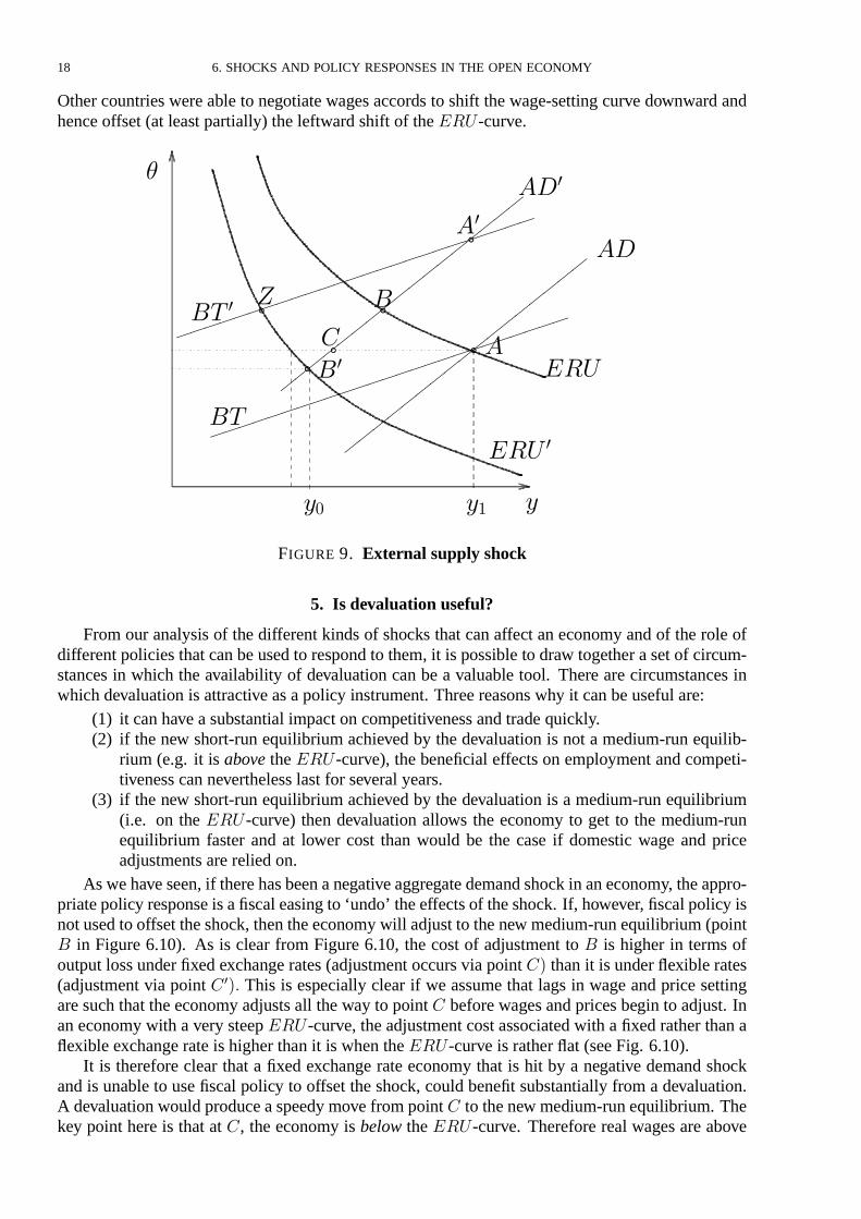
4.2. External supply shocks. An external supply shock is defined as an unanticipated changein the world terms of trade between manufactures and raw materials: a change in the world priceof oil is a good example. As noted in the previous section, this type of shock combines the effectsof an external trade shock with a supply-side impact on the price-setting real wage curve. Theconsequence is that there is a shift in the ��-curve, in the �� -curve and in the ��-curve: allcurvesshift in the samedirection.

��

��

��

��

��

�

��

�

��

�

�

�

�� " ��

�

�� " ��

��

��

��

FIGURE 8. A negative external supply shock: increase in the oil pr ice shifts�� -curve left

To see why the�� -curve shifts, we need to look closely at what is meant by a change in theworld price of oil. If we say that the world price of oil rises, this means that it rises relative to the

4. EXTERNAL TRADE AND SUPPLY SHOCKS 17

world price of manufactured goods, where " � � �

rm��

manuf . In other words, we are talking about achange in relativeprices, or to put it another way, achange in the real priceof oil. Theprice-settingcurve is defined for agiven real exchange rate, �. Now suppose that theworld price of oil rises. Foragiven �, a rise in thepriceof an essential input likeoil, raisescosts for firms in thehomeeconomyso if firms are to protect their profit margins, then real wages must be lower. Hence theprice-settingreal wage curve shifts downward when the world price of oil rises (see Fig. 6.8). This implies aleftward shift in the�� -curve as shown in Figure 6.8. The derivation of the price setting curveincorporating imported materials is presented in a footnote.7

We can now analyze the full impact of an exogenous and permanent change in the world priceof an essential commodity such as oil. We take the case of a rise in the price of oil. For simplicity,we assume that the home country only imports oil — it does not import final goods. This changesnothing essential and allows for a more direct examination of the issue at hand. We can investigatethe threeeffects:

(1) the impact on aggregatedemand(2) the impact on the tradebalance(3) the impact on priceand wagesetting and henceon the�� -curve.

We have already examined the first two effects in the analysis of an external trade shock inFigure6.7: there isadownward shock to net exportsbecause the increase in thecost of theessentialimported raw material absorbs a higher proportion of home income at a given real exchange rate.This shifts the�� curveand the�� curve to the left.8

We turn to the consequences of the shift in the ��-curve. The first observation is that thein�ationary consequences of the commodity price rise are clear. Following the external supplyshock, the initial equilibrium point � is above the new �� -curve. This means that at �� the realwage is below the wage-setting real wage. The reason is that the costs of home firms have gone upand higher domestic prices cut the real consumption wage.

In terms of the assessment of the adjustment paths under fixed and �exible exchange rates, it isclear that as compared with a pure external trade shock, the costs of the adjustment via exchangerate depreciation (higher in�ation via point �� in Fig. 6.9) go up relative to the costs of adjustmentwith a fixed exchange rate. This is clearly illustrated by reference to the two oil shocks in the1970s. In response to the first oil shock in 1973, many countries focused on the aggregate demandconsequencesand sought to offset them viaexpansionary fiscal and monetary policies. If we look attheconsequencesof anaccommodatingmonetary policy, thisallowed theexchangeratetodepreciate(to ��. The consequence was the onset of so-called stag�ation: rising unemployment and risingin�ation (as the economy eventually adjusted from �� to �� with unemployment rising and a burstof in�ation).

When the second oil shock struck in 1979, the nature of the shock was better understood andmany countries attempted to use tight monetary policy to prevent exchange depreciation and henceprevent a big upsurge in in�ation. In terms of Figure6.9, this allows adjustment from� to � to��.

7It is simplest to assume that there is no mark-up on imported materials. Assume the only imports are of rawmaterials. Then

��

where� � �� is the price of value added and � is unit materials requirement. This implies a price-setting real

wage:

��

� � ��

Any rise in � reduces the price-setting real wage. Note that any fall in unit materials requirement through increasedenergy efficiency, for example, would tend to offset this.

8Sincetheoil priceshock isa‘world’ phenomenon, therewill beafall in world aggregatedemand and world output,��, as all exporters of manufactures suffer from thesupply shock. This assumes — realistically — that the exporters ofraw materials, who have experienced an increase in their wealth, are unable to increase their expenditure sufficiently tocompensate. Thiswould reinforce the leftward shifts in the� and� curves.


Other countries wereable to negotiatewages accords to shift the wage-setting curve downward andhenceoffset (at least partially) the leftward shift of the�� -curve.

��

��

��

��

��

��

��

��

��

��

��

��

��

��

�

��

��

��

��

��

��

�

�

��

��

��

��

��

�

� �

��

��

��

FIGURE 9. External supply shock

5. Isdevaluation useful?

From our analysis of the different kinds of shocks that can affect an economy and of the role ofdifferent policies that can beused to respond to them, it ispossible to draw together aset of circum-stances in which the availability of devaluation can be a valuable tool. There are circumstances inwhich devaluation is attractiveas apolicy instrument. Three reasons why it can beuseful are:

(1) it can haveasubstantial impact on competitiveness and trade quickly.(2) if the new short-run equilibrium achieved by the devaluation is not a medium-run equilib-

rium (e.g. it is above the�� -curve), the beneficial effects on employment and competi-tiveness can nevertheless last for several years.

(3) if the new short-run equilibrium achieved by the devaluation is a medium-run equilibrium(i.e. on the �� -curve) then devaluation allows the economy to get to the medium-runequilibrium faster and at lower cost than would be the case if domestic wage and priceadjustments are relied on.

Aswehaveseen, if therehasbeen anegativeaggregatedemand shock in an economy, theappro-priatepolicy responseisafiscal easing to ‘undo’ theeffectsof theshock. If, however, fiscal policy isnot used to offset theshock, then theeconomy will adjust to thenew medium-run equilibrium (point� in Figure 6.10). As is clear from Figure 6.10, the cost of adjustment to � is higher in terms ofoutput lossunder fixed exchange rates (adjustment occursviapoint �� than it isunder �exible rates(adjustment via point � �� This is especially clear if we assume that lags in wage and price settingaresuch that theeconomy adjustsall the way to point � beforewagesand prices begin to adjust. Inan economy with a very steep�� -curve, theadjustment cost associated with a fixed rather than a�exibleexchange rate ishigher than it is when the��-curve is rather �at (seeFig. 6.10).

It is therefore clear that a fixed exchange rate economy that is hit by a negative demand shockand is unable to use fiscal policy to offset the shock, could benefit substantially from a devaluation.A devaluation would produceaspeedy movefrom point � to thenew medium-run equilibrium. Thekey point here is that at �, the economy is below the�� -curve. Therefore real wages are above

5. IS DEVALUATION USEFUL? 19

��

��

��

��

��

��

��

��

��

��

�

��

��

�� (�at)

�� (steep)

��

��

��

�

�

�

�

��

�

��

� �

FIGURE 10. Assessing the roleof devaluation

the level consistent with wage-setting equilibrium. Devaluation providesaquick way of cutting realwages: once the economy is on the ��-curve, in�ation will remain constant at the world rate.It is true that left to its own devices, the economy would move from point � to the medium runequilibrium (� or ��). But the process of disin�ation through successive rounds of wage and pricesetting could be extremely slow. Meanwhile, the economy suffers from unemployment higher thanconsistent with themedium run equilibrium.

We can draw a second lesson by combining the analysis of shifts in the �� -curve with theanalysisof theroleof exchangeratechanges. A supply-sidepolicy that shifts the�� -curve to theright allows the economy to move to a medium run position with lower unemployment. Howeveras noted above, the adjustment process may be very slow as wages and prices fall relative to worldprices over successive rounds of wage-setting. If the government has the possibility of devaluingthe exchange rate, a rapid shift to the new medium-run equilibrium is possible. The possibility ofdelivering quick results for employment may make it easier to gain approval for the supply-sidepolicy (e.g. a wages accord). The combination of wage accord and devaluation to accompanypolicies of fiscal consolidation was implemented by a number of European countries in the 1980s(seeChapter 16 for further details).

In the case of a negative external trade shock, we have argued that the correct policy responseis not to use fiscal policy to offset the shock since this widens the external imbalance. Under thesecircumstances, devaluation has something to commend it as an interim measure. Devaluation helpsto mitigate the impact of the external trade shock on output and on the trade balance. Of course, itonly provides a temporary solution since the devaluation takes the economy above the�� -curveby cutting real wages. Thebenefits to competitivenesswill beeroded in subsequent wageand price-setting rounds. However, in the face of a temporary external trade shock devaluation could proveuseful. If theexternal tradeshock signifiesamoreseriousunderlying problem for theeconomy suchasashift in tastesaway from thegoods that thehomeeconomy specializes in, then devaluation maydivert the attention of both private and public sector actors from the source of the problem in thesupply-sideof theeconomy.


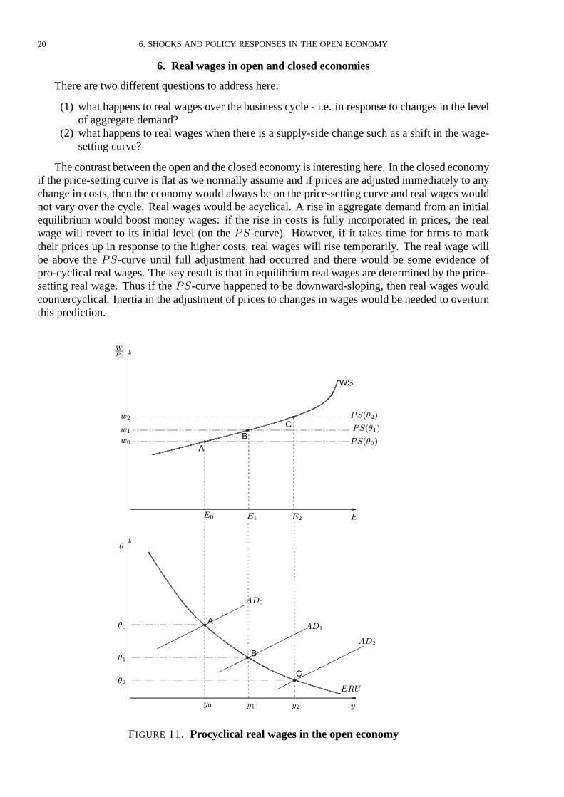
6. Real wages in open and closed economies

Thereare two different questions to addresshere:

(1) what happensto real wagesover thebusinesscycle- i.e. in response to changes in the levelof aggregatedemand?

(2) what happens to real wages when there isasupply-sidechangesuch asashift in thewage-setting curve?

Thecontrast between theopen and theclosed economy isinteresting here. In theclosedeconomyif theprice-setting curve is�at aswenormally assumeand if pricesareadjusted immediately to anychange in costs, then theeconomy would alwaysbeon theprice-setting curveand real wageswouldnot vary over the cycle. Real wages would be acyclical. A rise in aggregate demand from an initialequilibrium would boost money wages: if the rise in costs is fully incorporated in prices, the realwage will revert to its initial level (on the ��-curve). However, if it takes time for firms to marktheir prices up in response to the higher costs, real wages will rise temporarily. The real wage willbe above the ��-curve until full adjustment had occurred and there would be some evidence ofpro-cyclical real wages. Thekey result is that in equilibrium real wagesaredetermined by theprice-setting real wage. Thus if the��-curve happened to be downward-sloping, then real wages wouldcountercyclical. Inertia in theadjustment of prices to changes in wageswould beneeded to overturnthis prediction.

��

��

��

��

��

�� BC

WS

��

��

��

��

��

�

A

B

�

A

��

��

��

C

��

�

�

�

�

��

��

��

��

FIGURE 11. Procyclical real wages in theopen economy

6. REAL WAGES IN OPEN AND CLOSED ECONOMIES 21

By contrast in the open economy, what happens to real wages in response to different shocksdepends on the exchange rate regime and on the nature of the shock, as well as on the lags in wageand price-setting and the slope of the ��-curve. As we have already seen, in the open economyprocyclical real wages in the medium-run are likely to be observed following an �� shock (e.g.consumption, investment, government spending, taxation) as theeconomy settles at anew medium-run equilibrium on the��-curve. Theeconomy movesup the �-curve in theevent of apositiveshock and down in the event of a negative shock. Fig. 6.11 illustrates: the rise in employment from�� to�� to�� is associated with a rise in real wages from�� to�� to��.

Of course, if activity �uctuates because of changes in monetary policy then the economy willmovealong the�� curve. A loosening of monetary policy (associated with adepreciation) will leadto a rise in output and a rise in competitiveness (�). This entails a fall in the real wage. Thus with�uctuationscoming from�� shifts, real wageswill movecountercyclically. Unlikethe�uctuationsassociated with �� shifts, movements along the�� curvewill only beobserved in theshort run.

In the closed economy supply side policies that shift only the wage-setting curve have no effecton the medium run real wage. Figure 6.12 illustrates this by taking the case of a downward shiftin the �-curve. This could have been the result of a labour market reform that weakened unionbargaining power or it could havebeen dueto thenegotiation of asocial pact. Either way if the �-curve shifts down, the equilibrium unemployment rate falls but real wages remain unchanged at thenew �� at point �. Equilibrium employment rises becauseof the reduction in wagepressureandnot because of a reduction in real wages.

��

��

��A

�

E

��

��

��B

� �

(a) Closed economy

�

��

A B��

” ��”

E

��

��

(b) Open economy

��

”��”

”�� ”

��

��

C

FIGURE 12. Supply-sidepolicy and real wages: compar ing the closed and open economies.

How does a downward shift in the � curve affect real wages in the open economy? The��-curve and the �� -curve are shown in the real wage/employment diagram and labelled as “��”and “�� ” respectively. In an open economy, a similar result can be achieved to that in the closedeconomy if the downward shift in the �-curve is accompanied by an expansionary fiscal policyso that the �� curve moves to the right to �� . Higher employment would be achieved withoutany fall in actual real wages. But unlike the closed economy, this is not sustainable in the long runin the open economy. At �, there is a trade deficit. The real wage has to fall to �� to eliminatethe deficit, and this requires a trimming back of the employment gain (point �). Exchange ratedepreciation plus a tightening of fiscal policy will achieve this. The fundamental point is that in anopen economy, a rise in employment can only be sustained in the long run by a fall in real wages,


even if such afall isnot required to makeproduction profitable(i.e. even when the��-curveis�at).The fall in real wages is necessary to raise competitiveness (from �� to ��) and secure a satisfactoryexternal account.

7. Conclusions

In thischapter thebasic model hasbeen used to examinetheimpact on theeconomy of aseriesofdifferent kindsof policiesand shocks. Fiscal policy, monetary/exchangeratepolicy and supply-sidepolicy havebeen investigated.

� Aggregate demand shocks that shift the��-curve and therefore the medium run equilib-rium are changes in autonomous consumption and investment. The short-run effects of anaggregatedemand shock can bebest offset by using fiscal policy.

� Changes in monetary policy in a �exible exchange rate regime or discrete changes in theexchange rate peg in a fixed rate system lead to a shift along the��-curve and thereforedo not change themedium run equilibrium

� Supply shocksand supply-sidepoliciesaredefinedasthosethat shift either thewage-settingcurve, theprice-setting curve(for agiven real exchangerate) or both. In theopen economy,asupply shock or policy isone that shifts the�� -curveand henceshifts themedium andlong run equilibrium rateof unemployment.

� External trade shocks are defined as those that change the level of net exports for a givenreal exchange rate. Such shocks shift the�� and the�� -curves and therefore change theshort, medium and long run equilibria.

� External supply shockssuch asachange in theworld priceof an essential commodity shiftthe��, �� and�� curves.

� Theusefulnessof devaluation asapolicy instrument dependson thenatureof theshock, thestarting position of the economy (e.g. on or off the��-curve), the structural character-istics of theeconomy (e.g. the lags in wage and price setting and the responsiveness of thewage-setting real wageto changesin unemployment) and theavailability of complementarypolicies (e.g. fiscal policy, supply-sidepolicies).

� The model predicts that there will not be a fixed relationship between real wages and em-ployment e.g. pro-cyclical or counter-cyclical real wages in theopen economy. Thepatternwill depend on thenature of theshock (e.g. ��-shock, �� -shock or supply-sideshock).

1. APPENDIX: OPEN ECONOMY INFLATION AND SHORT-RUN PHILLIPS CURVES: AN EXAMPLE 23

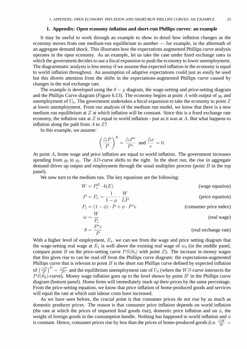
1. Appendix: Open economy in�ation and short-run Phillips curves: an example

It may be useful to work through an example to show in detail how in�ation changes as theeconomy moves from one medium-run equilibrium to another — for example, in the aftermath ofan aggregatedemand shock. This illustrateshow theexpectationsaugmented Phillipscurveanalysisoperates in the open economy. As an example, let us take the case under fixed exchange rates inwhich thegovernment decidestouseafiscal expansion topush theeconomy to lower unemployment.Thediagrammatic analysisislessmessy if weassumethat expected in�ation in theeconomy isequalto world in�ation throughout. An assumption of adaptive expectations could just as easily be usedbut this diverts attention from the shifts in the expectations-augmented Phillips curve caused bychanges in the real exchange rate.

The example is developed using the � � diagram, the wage-setting and price-setting diagramand the Phillips Curvediagram (Figure 6.13). Theeconomy begins at point � with output of � andunemployment of ��. Thegovernment undertakesafiscal expansion to take theeconomy to point �at lower unemployment. From our analysis of the medium run model, we know that there is a newmedium run equilibrium at � at which in�ation will be constant. Since this is a fixed exchange rateeconomy, the in�ation rateat � isequal to world in�ation - just as it was at �. But what happens toin�ation along thepath from� to�?

In thisexample, weassume:��

�

��

� �and

�

��

At point �, home wage and price in�ation are equal to world in�ation. The government increasesspending from �� to �� The ��-curve shifts to the right. In the short run, the rise in aggregatedemand drives up output and employment through the usual multiplier process (point � in the toppanel).

Wenow turn to themedium run. Thekey equations are the following:

� �� (wageequation)

� � ��

��

��(priceequation)

�� (consumer price index)

� �

��(real wage)

� ��

�(real exchange rate)

With a higher level of employment, �� we can see from the wage and price setting diagram thatthe wage-setting real wage at �� is well above the existing real wage of �� (in the middle panel,compare point � on the price-setting curve �� with point �). The increase in money wagesthat this gives rise to can be read off from the Phillips curve diagram: the expectations-augmentedPhillips curve that is relevant to point � is theshort run Phillips curvedefined by expected in�ationof��

�

��

� �and theequilibrium unemployment rateof �� (where the �-curve intersects the

��-curve). Money wage in�ation goes up to the level shown by point �� in the Phillips curvediagram (bottom panel). Homefirmswill immediately mark up their pricesby thesamepercentage.From the price-setting equation, we know that price in�ation of home-produced goods and serviceswill equal the rate at which unit labour costshave increased.

As we have seen before, the crucial point is that consumer prices do not rise by as much asdomestic producer prices. The reason is that consumer price in�ation depends on world in�ation(the rate at which the prices of imported final goods rise), domestic price in�ation and on �, theweight of foreign goods in the consumption bundle. Nothing has happened to world in�ation and �isconstant. Hence, consumer pricesriseby lessthan thepricesof home-produced goods(i.e. ��

��


��

��

��

��

��

��

��

��

��

��

��

��

��

��

��

��

��

��

��

��

��

�

�

��

�

�

��

�

��

�

��

��

��

��

��

��

�

��

��

��

�

��

��

��

��

��

��

FIGURE 13. Expectationsaugmented Phillipscurves in theopen economy: tem-porary r isein in�ation following a loosening of fiscal policy under fixed exchangerates.

��

�# ��

��# ��

� �) which implies that the real wage

��

�increases and price competitiveness ��

decreases. In Figure 13, the real wage rises from�� to ��and � falls from �� to ��. Theeconomy isnow at point � in Figure6.13 (seetheupper two panels). Theupward shift of theprice-setting curveisshown in thecentral panel: thismeansthat theequilibrium rateof unemployment hasdecreased to�� . A new expectations-augmented Phillipscurvemust thereforebedrawn: it is indexed by the levelof � (i.e. ��) and shows that in the following period, money wages will rise by less thanin the previous period. The reason is straightforward: the real wage has risen closer to the value ofthewage-setting real wageat ��. Thus there is less discrepancy between the real wage that workersanticipateand thewage they actually receive, which in turn means that wage in�ation has to exceedexpected in�ation by asmaller percentage.

In subsequent periods, wages and prices increase according to the above pattern (i.e.��

��

�# ��

��# ��

�� and � �) until the real wage is equal to � and the real exchange rate is

equal to � . The economy will then be at the new medium run equilibrium at point �. At point �,

2. APPENDIX: THE PRICE-SETTING CURVE IN THE OPEN ECONOMY WITH TAXES 25

��

��

��

��

� �and there is constant in�ation at the lower unemployment rate, ��. The

real wageand the real exchange rate remain constant at thevalues� � � .

2. Appendix: Thepr ice-setting curve in theopen economy with taxes

Thewageelement of costs for firmsis thefull cost of labour to firms- i.e. thegrosswagepaid totheworker (which includes the incometax and social security payments that have to bemadeby theworker) plus the employer’s social security contributions. All of these direct taxes are summarizedin the tax rate, ��. This is shown in thepricing equation:

� � ��

��

��(priceequation)

��

��

��

In order to derive the price-setting real wage, it is necessary to note that we must express the price-setting real wage in terms of the real consumption wage, �

��. We use the definition of the consumer

price index as before, but include value added tax at the rate �� The home country’s VAT is leviedon imported final goods.

�� (consumer price index)After sometediousalgebraic manipulation, which isshown in thefootnote, wederivetheexpressionfor theprice-setting real wage in theopen economy including tax variables:9.

��

�� (price-setting real wage, open)

Although this expression looks frightening, it is very easy to interpret. It is simply the usual openeconomy price-setting real wage adjusted for the so-called tax wedge. Any increase in either di-rect or indirect taxation reduces the price-setting real wage and therefore shifts the ��-curvedownwards.

9Divide�� by �

��

� � ��

��

� ��

�

��

therefore� � ��

��

��

��

��

�

��

��

��

��

��

shocks and policy responses in the open economyuctpa36/ch6feb03.pdf · chapter 6 shocks and policy...

Documents