shoreline characterization report - okanogan county

Appendix A.1 Okanogan County

Shoreline Characterization

Prepared for Okanogan County

Prepared by ENTRIX, Inc

148 Rogers St. NW Olympia, WA 98502

November 20, 2008

Okanogan County SMP

[ THIS PAGE IS INTENTIONALLY BLANK ]

TABLE OF CONTENTS

1 Introduction ........................................................................................................................... 3 1.1 Purpose................................................................................................................ 3 1.2 Shoreline Jurisdictional Area.............................................................................. 3

1.2.1 Streams........................................................................................................ 3 1.2.2 Stream Shorelines of Statewide Significance ............................................. 3 1.2.3 Columbia River Impoundments.................................................................. 4 1.2.4 Lakes ........................................................................................................... 4 1.2.5 Lake Shorelines of Statewide Significance................................................. 4

2 Regional Setting.................................................................................................................... 5 2.1 Climate................................................................................................................ 5 2.2 Topography......................................................................................................... 5

2.2.1 Hydrology ................................................................................................... 6 2.3 Vegetation ........................................................................................................... 6 2.4 Wildlife ............................................................................................................... 7 2.5 Geology............................................................................................................... 8 2.6 Land Uses............................................................................................................ 8

3 Analysis Methods ................................................................................................................. 9 3.1 Analysis Overview.............................................................................................. 9 3.2 Site-Scale Analysis ............................................................................................. 9

3.2.1 Define Analysis Units ................................................................................. 9 3.2.2 Shoreline Function Calculations ............................................................... 11 3.2.3 Aggregate Condition Index....................................................................... 11 3.2.4 Aggregate Resource Index........................................................................ 19 3.2.5 AU Characterization Quadrant Analysis .................................................. 28

3.3 Watershed-Scale Analysis ................................................................................ 28 3.3.1 Watershed Boundaries .............................................................................. 29

4 Characterization Results.................................................................................................... 31 4.1 Introduction....................................................................................................... 31 4.2 AU Characterization Results Catalog ............................................................... 31 4.3 Characterization Quadrant Analysis Results .................................................... 31 4.4 Potential Use of Quadrant Analysis.................................................................. 34 4.5 Summary ........................................................................................................... 35

5 Continued Science Support for SMP Update................................................................... 36 5.1 Environmental Designation Determination ...................................................... 36 5.2 Cumulative Effects............................................................................................ 36 5.3 Restoration Plan ................................................................................................ 36

6 References........................................................................................................................... 37 Appendix A.2: AU Results Catalog Appendix A.3: Tables Appendix A.4: Map Portfolio

Okanogan County Shoreline Characterization i

Okanogan County SMP

LIST OF FIGURES

Figure 1: Conceptual model of inputs to ecosystem function............................................ 9 Figure 2 Conceptual interpretation of Quadrant Assignments; analysis unit condition index vs. resource index.................................................................................................... 28 Figure 3 Plot of AU condition and resource indices, Okanogan County, WA (n=233).. 32 Figure 4 Modified AU condition and resource indices’ plot showing approximate location of quadrant boundaries for Characterization results ........................................... 33 Figure 5 Graphic example representing AUs near the Middle Methow River by quadrant assignment......................................................................................................................... 34

LIST OF TABLES Table 1 Analysis Unit Stressor Scoring and Weighting ................................................... 16 Table 2 Example of Variation in Index Weighting Based on Data Availability .............. 18 Table 3 Species Included in AU Resource Scoring .......................................................... 20 Table 4 Analysis Unit Resource Scoring and Weighting ................................................. 24 Table 5 Weighting of Lake and Stream AUs.................................................................... 27

ii Okanogan County Shoreline Characterization

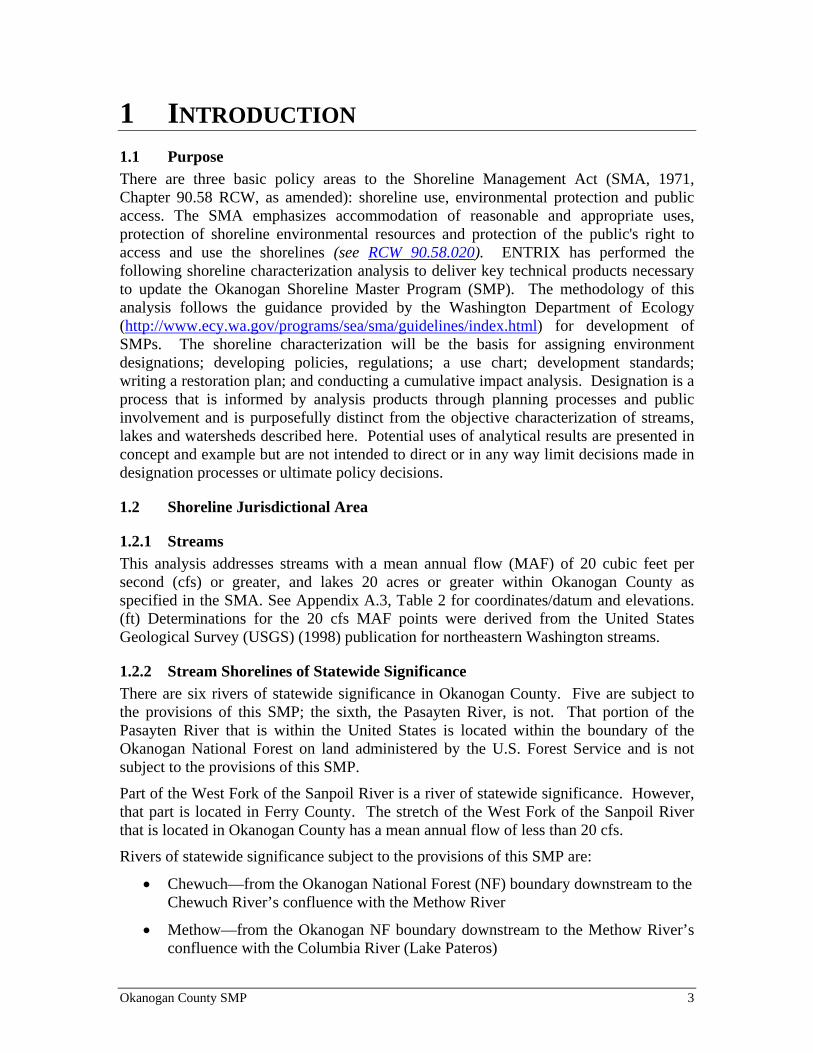
1 INTRODUCTION 1.1 Purpose There are three basic policy areas to the Shoreline Management Act (SMA, 1971, Chapter 90.58 RCW, as amended): shoreline use, environmental protection and public access. The SMA emphasizes accommodation of reasonable and appropriate uses, protection of shoreline environmental resources and protection of the public's right to access and use the shorelines (see RCW 90.58.020). ENTRIX has performed the following shoreline characterization analysis to deliver key technical products necessary to update the Okanogan Shoreline Master Program (SMP). The methodology of this analysis follows the guidance provided by the Washington Department of Ecology (http://www.ecy.wa.gov/programs/sea/sma/guidelines/index.html) for development of SMPs. The shoreline characterization will be the basis for assigning environment designations; developing policies, regulations; a use chart; development standards; writing a restoration plan; and conducting a cumulative impact analysis. Designation is a process that is informed by analysis products through planning processes and public involvement and is purposefully distinct from the objective characterization of streams, lakes and watersheds described here. Potential uses of analytical results are presented in concept and example but are not intended to direct or in any way limit decisions made in designation processes or ultimate policy decisions.

1.2 Shoreline Jurisdictional Area

1.2.1 Streams This analysis addresses streams with a mean annual flow (MAF) of 20 cubic feet per second (cfs) or greater, and lakes 20 acres or greater within Okanogan County as specified in the SMA. See Appendix A.3, Table 2 for coordinates/datum and elevations. (ft) Determinations for the 20 cfs MAF points were derived from the United States Geological Survey (USGS) (1998) publication for northeastern Washington streams.

1.2.2 Stream Shorelines of Statewide Significance There are six rivers of statewide significance in Okanogan County. Five are subject to the provisions of this SMP; the sixth, the Pasayten River, is not. That portion of the Pasayten River that is within the United States is located within the boundary of the Okanogan National Forest on land administered by the U.S. Forest Service and is not subject to the provisions of this SMP.

Part of the West Fork of the Sanpoil River is a river of statewide significance. However, that part is located in Ferry County. The stretch of the West Fork of the Sanpoil River that is located in Okanogan County has a mean annual flow of less than 20 cfs.

Rivers of statewide significance subject to the provisions of this SMP are:

• Chewuch—from the Okanogan National Forest (NF) boundary downstream to the Chewuch River’s confluence with the Methow River

• Methow—from the Okanogan NF boundary downstream to the Methow River’s confluence with the Columbia River (Lake Pateros)

Okanogan County SMP 3

http://apps.leg.wa.gov/rcw/default.aspx?cite=90.58.020

http://www.ecy.wa.gov/programs/sea/sma/guidelines/index.html

Okanogan County SMP

• Okanogan—from the Canadian border to the Okanogan River’s confluence with the Columbia River (Lake Pateros—the entire length of the Okanogan River within the United States)

• Similkameen—from the Canadian border to the Similkameen River’s confluence with the Okanogan River (the entire length of the Similkameen River within the United States)

• Twisp—from the Okanogan NF boundary downstream to the Twisp River’s confluence with the Methow River

1.2.3 Columbia River Impoundments The shorelines of the Columbia River are shorelines of state-wide significance. There are three impoundments on the Columbia River that are partially located within Okanogan County. One, Lake Pateros, is subject to the provisions of this SMP; the other two are not, as explained below. Columbia River impoundments that are not subject to the provisions of this SMP:

• Franklin D. Roosevelt Lake—Franklin D. Roosevelt Lake is that portion of the Columbia River that is impounded behind Coulee Dam. The lake forms the boundary between Okanogan County to the north and Grant and Lincoln counties to the south. That portion of the shoreline of Franklin D. Roosevelt Lake that is located within Okanogan County is also located within the boundary of the Colville Indian Reservation and so is not subject to the provisions of this SMP.

• Rufus Woods Lake—Rufus Woods Lake is the portion of the Columbia River that is impounded behind Chief Joseph Dam. The lake forms a portion of the boundary between Okanogan County to the north and Douglas County to the south. The portion of the shoreline of Rufus Woods Lake that is located within Okanogan County is also located within the boundary of the Colville Indian Reservation and so is not subject to the provisions of this SMP.

1.2.4 Lakes Lakes were identified using existing GIS data on file with Okanogan County and proofed for accuracy by knowledgeable local experts. The requirements of the SMA apply to private projects on privately owned lands, and to private, local government, and state government actions on local or state government lands. Shorelines on federal and tribal lands are not included in this analysis.

1.2.5 Lake Shorelines of Statewide Significance There are three lakes of statewide significance in Okanogan County. Two are subject to the provisions of this SMP. The third, Omak Lake, is located within the boundary of the Colville Indian Reservation and is not subject to the provisions of this SMP. Lakes of statewide significance subject to the provisions of this SMP are:

• Lake Osoyoos

• Palmer Lake

4 Okanogan County Shoreline Characterization

2 REGIONAL SETTING 2.1 Climate Okanogan County’s climate is arid to semiarid, characterized by hot, dry summers and cold winters. The county is located directly east of the crest of the Cascade Range, a major mountain range extending from southern British Columbia to northern California. The range acts as a barrier to marine air moving eastward from the Pacific Ocean. It also exerts a rain-shadow effect, resulting in heavy precipitation at high elevations. Precipitation rates throughout the county are a function of elevation and of distance from the Cascade crest, and vary widely, from less than 10 inches along the Columbia River to 80-100 inches or more in the Cascades.

Most of the land subject to this SMP is at relatively low elevation; precipitation ranges from 8 to 35 inches per year, on average, with most falling from October through March. However, many of the county’s rivers, streams, and lakes are fed by runoff from higher elevations, where much of the annual precipitation is retained as snowpack and released during the spring and summer months.

2.2 Topography Okanogan County topography ranges from mountainous alpine and sub-alpine terrain to gently sloping valleys. Elevation varies from over 8,500 feet in the Cascade Range to approximately 750 feet where the Columbia River crosses the County line south of Pateros.

The landscape below 5,000 feet was sculpted by glaciers about 10,000 years ago. Large areas remain covered with rocks and other sediments deposited by glaciers or by rivers and lakes that formed when the glaciers began to melt. While most soils are coarsely textured and fast draining, volcanic ash and fine-textured sediments have contributed to less permeable soils in some places.

Where impermeable soil layers occur, they have sometimes created perched aquifers—areas of groundwater that are not connected to rivers and streams. However, in most parts of Okanogan County, groundwater is connected to rivers and streams. Groundwater flows into those water bodies during periods when soil moisture is high (generally during the spring snow-melt season). When moisture levels are low, water moves out of rivers and streams to replenish groundwater.

Because soils are generally coarse (which means water moves through them quickly and easily), and because most water is available for a short period every year, river and stream levels tend to fluctuate a great deal, rising and even overtopping streambanks in the spring, and dropping so low in the summer and fall that some stream segments become completely dry. Healthy riparian areas can help retain water so that it is more available during the dry season. Water that is held in floodplains and wetlands can seep into soils far from streams and lakes, helping to keep wells productive year round, as well as feeding the water bodies themselves.


Okanogan County SMP

2.2.1 Hydrology The Soil Survey of Okanogan County Area provides a good introduction to Okanogan County’s hydrology:

[Okanogan County] is drained by two principal streams—the Okanogan river and the Methow River. All the drainage water ultimately flows into the Columbia River. The Okanogan is a slow flowing, meandering stream that drains the eastern part of the Area. A considerable part of its flow originates in Canada. The Methow River is a clear, fast flowing stream that drains the western part of the Area…. Okanogan County is well supplied with lakes at all elevations.

As noted above, river and stream flows and some lake levels vary seasonally. Flow rates are highest in the spring when snow is melting fast. Snow melt continues to supply rivers and streams with water through much of the year. (Even after most of the snow is gone, melted snow continues to percolate through the soil to the groundwater and perched aquifers, supplying rivers, streams, lakes, and wells with water.)

Shoreline ecological health is very important because it determines how much water stays in local watersheds and for how long. Shoreline vegetation and wetlands help hold water and allow it to seep gradually into water bodies.

Because Okanogan County is arid, availability of water is very important. Both the economy and the ecosystem are dependent on water resources. Agriculture, an important component of the local economy, depends on irrigation. Sources of irrigation water include groundwater, rivers and streams, and lakes and impoundments.

2.3 Vegetation Okanogan County is generally forested at higher elevations, with shrub-steppe habitat dominating the landscape at lower elevations. Shoreline areas and other wet areas support riparian and wetland vegetation.

As noted above, most of the land subject to this SMP is at relatively low elevation; however, this SMP does apply to some forested areas. In those areas, ponderosa pine (Pinus ponderosa) generally dominates at lower elevations, where annual precipitation ranges from 14-16”; Douglas-fir (Pseudotsuga menziesii) is dominant in areas with higher levels of precipitation.

Forested areas are subject to fire, and years of fire suppression have resulted in heavy fuel loads. Severe fires have been relatively common in recent years. Forest fires affect runoff and sedimentation patterns and may have significant effects on shoreline areas.

Sagebrush, rabbitbrush, and bitterbrush are the dominant native plant species in much of the county’s shrub steppe. In the driest areas, where annual precipitation is below 15”, grasses (including Idaho fescue, bluebunch wheatgrass, and wild rye) become more important.


Okanogan County SMP

Trees common to riparian areas are cottonwood, aspen, water birch, and alder; shrubs include willows, dogwood, spirea, hawthorne, rose, and snowberry. Grasses, forbs, and other herbaceous plants (cattails, for instance) dominate many wetlands. Wetland and riparian vegetation is often quite dense; it helps to retain water in shoreline areas and provides food and cover for wildlife.

Invasive plant species are a problem in some areas, competing with native species and diminishing habitat value.

2.4 Wildlife Okanogan County is home to several hundred species of amphibians, birds, fish, mammals, and reptiles, as well as numerous invertebrates (animals without backbones, such as insects and spiders).

Some of the animals found in the county are listed below:

• Amphibians: frogs, newts, salamanders, and toads.

• Birds: migratory and resident species include marine species, herons, waterfowl, hawks, falcons, eagles, corvids, upland game birds, cranes, shorebirds, owls, woodpeckers, hummingbirds, and perching birds (e.g., sparrows, orioles, grosbeaks).

• Fish: anadromous and resident, including three federally-listed species: spring Chinook, summer steelhead, and bull trout. Many lakes and streams also support introduced species that compete with native fish.

• Invertebrates: butterflies, beetles, mollusks, spiders, ticks, and benthic macroinvertebrates (stream-dwelling animals that are important food sources for fish).

• Mammals: ungulates, including deer, moose, elk, mountain goat, and bighorn sheep; carnivores such as cougar, lynx, wolf, coyote, bobcat, bear, wolverine, and ermine; rodents, including squirrels, gophers, moles, voles, and mice; lagomorphs (rabbits and hares), including snowshoe hare; shrews; and bats. The Methow subbasin is home to the State’s largest migratory mule deer herd.

• Reptiles: lizards, turtles, snakes

Game species, especially deer, are very important to the local economy.

The biotic structure and composition of shorelines (including aquatic, riparian, and nearby wetland areas) depend largely on the hydrologic regime. The annual variation in hydrology is essential to many species life-cycle and necessary to sustain biodiversity and plays a role in population dynamics (Mitsch and Gosselink, 2000). Most animals use these shoreline areas and some spend their entire lives there. Wetlands and other shoreline areas provide important habitat for migratory birds, including those that nest and raise young in the county and those that pass through en route to and from more northerly nesting grounds.

Okanogan County Shoreline Characterization 7

Okanogan County SMP

Okanogan County’s wildlife population includes a number of species designated by the Washington Department of Fish and wildlife as priority species—those that “require protective measures for their perpetuation due to their population status, sensitivity to habitat alteration, and/or recreational, commercial, or tribal importance. Priority species include State Endangered, Threatened, Sensitive, and Candidate species; animal aggregations considered vulnerable; and those species of recreational, commercial, or tribal importance that are vulnerable.” The County’s land base also includes priority habitats—“those habitat types or elements with unique or significant value to a diverse assemblage of species. A priority habitat may consist of a unique vegetation type or dominant plant species, a described successional stage, or a specific structural element.”

The hydroelectric facilities on the Columbia River have had very significant impacts on fish and wildlife, particularly on anadromous salmonids, several species of which breed and rear young in Okanogan County streams.

2.5 Geology The geology of the area is complex, developed from marine invasions, volcanic deposits, and glaciations. The area consists of four differing geologic provinces. The Cascade Range, to the west, was created by ancient seabed uplift. Both the Okanogan highlands on the east and the Columbia basalt plateau to the south were created by volcanic activity. Finally, the oldest is the ridge of ancient seabed rocks that were folded and then carved by erosion into its present forms. During the ice age, ice spread over these dissimilar landforms and when receded, left valleys, canyons, waterfalls, benches, and cliffs (Widel, 1973).

2.6 Land Uses Okanogan County is the largest county in Washington, comprising 5,821 square miles—almost 8% of the state’s land mass. Development in Okanogan County is concentrated in the Methow and Okanogan valleys and along the Columbia River. The mountainous areas to the west of the Methow valley and between the Methow and Okanogan valleys are mostly federally-owned. Mining, forestry, agriculture, and recreation are the major land-use activities. Residential development is also significant. Much of that development is attributable to non-resident landowners building vacation houses, and so is not reflected in population statistics.


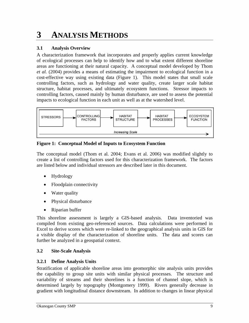
3 ANALYSIS METHODS 3.1 Analysis Overview A characterization framework that incorporates and properly applies current knowledge of ecological processes can help to identify how and to what extent different shoreline areas are functioning at their natural capacity. A conceptual model developed by Thom et al. (2004) provides a means of estimating the impairment to ecological function in a cost-effective way using existing data (Figure 1). This model states that small scale controlling factors, such as hydrology and water quality, create larger scale habitat structure, habitat processes, and ultimately ecosystem functions. Stressor impacts to controlling factors, caused mainly by human disturbance, are used to assess the potential impacts to ecological function in each unit as well as at the watershed level.

Figure 1: Conceptual Model of Inputs to Ecosystem Function

The conceptual model (Thom et al. 2004; Evans et al. 2006) was modified slightly to create a list of controlling factors used for this characterization framework. The factors are listed below and individual stressors are described later in this document.

• Hydrology

• Floodplain connectivity

• Water quality

• Physical disturbance

• Riparian buffer

This shoreline assessment is largely a GIS-based analysis. Data inventoried was compiled from existing geo-referenced sources. Data calculations were performed in Excel to derive scores which were re-linked to the geographical analysis units in GIS for a visible display of the characterization of shoreline units. The data and scores can further be analyzed in a geospatial context.

3.2 Site-Scale Analysis

3.2.1 Define Analysis Units Stratification of applicable shoreline areas into geomorphic site analysis units provides the capability to group site units with similar physical processes. The structure and variability of streams and their shorelines is a function of channel slope, which is determined largely by topography (Montgomery 1999). Rivers generally decrease in gradient with longitudinal distance downstream. In addition to changes in linear physical


Okanogan County SMP

characteristics, some biological characteristics are also predictable (Vannote et al. 1980). Since slope is a controlling factor on channel morphology and physical habitat, slope was used as one of the primary variables to classify Aus within Okanogan County.

The concept here is that analysis units of similar geomorphology (e.g., broad valley bottoms with extensive floodplains) attract specific types of development within shoreline areas that are likely to require similar designations under the SMA. By stratifying the shoreline areas into relatively homogenous analysis units, resulting characterizations are most meaningful and consistent and a ready link between science and policy is provided for public input and discussion. While data are not available at this time to provide a comprehensive geomorphic classification of each site, three variables are used to provide a useful geomorphic context for the definition of analysis unit (AU) boundaries of the County’s SMP jurisdictional rivers: slope classes, stream order, and stream sinuosity. As noted above, shorelines within Okanogan County that are on federal or tribal lands are not included in this analysis.

The Aus in this analysis are based on interpretations from a low-resolution digital elevation models (DEM) and general, published geologic maps. ENTRIX or its employees are not responsible for specific delineation boundaries in any way unless and until a thorough analysis that includes higher resolution mapping, photogrammetric interpretation, and field calibration is accomplished. Provision of such a rigorous analysis for delineation of Aus was beyond the scope and budget of this project. Analysis units are provided as a general guide to channel conditions based on available information and are not intended for use in other jurisdictional delineations.

Slope classes were based on slope gradients that can be estimated from DEMs. These classes were broken into categories of 0 to 2 percent, 2 to 4, and over 4 percent. Stream order is a measure of the relative size of streams that range from the smallest (first-order), to the largest (twelfth-order). In Okanogan County, the shoreline jurisdiction encompasses stream orders from third-order to fifth-order.

Stream sinuosity is a river’s tendency to move back and forth across the floodplain, in an S-shaped pattern, over time (Leopold, 1994). The variation of steam sinuosity is characterized by a number within the range of 0 to 1, with 0 representing no sinuosity and 1 representing high sinuosity. All the characteristics were based on re-projected, filled 10-meter DEMs of Okanogan County. Data on hillshade, flow direction, flow accumulation, streams, stream order and slope were all derived from these DEMs.

Lakes of 20 acres or more were analyzed as individual units. Lakes greater than 200 acres were subdivided longitudinally into separate Aus and by bathymetry. Large lakes and reservoirs were then divided lengthwise based on the knowledge that shorelines on either side of large water bodies may be dissimilar. Bathymetry provides an indication of shallow shorelines where emergent vegetation would grow verses shorelines with deeper water.

Shorelands are under the Jurisdiction of the SMA and are defined in relation to geographic proximity to stream and lake shorelines (WAC 173-22-040). All Aus were


Okanogan County SMP

then given a 200 foot buffer to include shorelands extending landward above the ordinary high water mark (OHWM). All wetlands within or associated with the 200 foot buffer are considered jurisdictional and are included in the Aus.

Associated wetlands beyond the 200 foot buffer were included in the SMA because significant amounts of water are exchanged laterally (saturated sediments beneath the stream channel) with saturated sediments surrounding the stream and riparian areas. This process has been defined as the hyporehic zone but only recently been researched as to the importance both chemically and biologically (Brunke and Gonser, 1997; Findlay, 1995).

3.2.2 Shoreline Function Calculations For each AU, two estimates of shoreline function were calculated; an aggregate condition index and an aggregate resource index. The following steps were taken to calculate the aggregate condition index:

• Step 1: Identification of AU Stressors

• Step 2: Scoring of AU Stressors

• Step 3: Weighting of AU Stressors

• Step 4: Calculation of AU Condition Index

Much in the same way as the calculation index, the following steps were taken to calculate the aggregate resource index:

• Step 1: Identification of AU Resources

• Step 2: Scoring of AU Resources

• Step 3: Weighting of AU Resources

• Step 4: Calculation of AU Resource Index

The details of each of these steps and examples are provided in the text below.

3.2.3 Aggregate Condition Index

Step 1: Identification of AU Stressors An evaluation of the main ecological impacts, or stressors, was performed in order to assess the ecological condition of each AU. The stressor data used in this analysis were drawn from a pool of potential stressors to shoreline function. Ideally, important and influential stressors would be readily available and represented in extant data sets. However, through the process of data inventory, a set of potential stressors was identified that provide a direct linkage to, or index of, factors that are controlling or likely to significantly affect ecological function.

Bank Hardening. Bank hardening (e.g., riprap) stresses the shoreline by limiting riparian function, disconnecting the floodplain and limiting the lateral movement of the river channel. To prevent stream bank erosion, riprap, has been used for over a century.


Okanogan County SMP

Most of these activities were unregulated prior to the recognition of potential environmental impact of bank hardening activities (Fischenich, 2003). Data on bank hardening, specifically riprap, were provided by Golder and Associates (Golder 2007), who completed a field survey of man-made structures along the mainstem of Okanogan River for Okanogan County. Aus with insufficient data on bank hardening were not analyzed for this stressor.

Levees. Levees also stress the shoreline by limiting riparian function, disconnecting the floodplain and limiting the lateral movement of the river channel. Data on levees were provided by Golder and Associates, who completed a field survey of man-made structures along the mainstem of Okanogan River for Okanogan County. Additionally, further levee dimensions were provided in digital form from Highland Associates based on local knowledge. Aus with insufficient data on levees were not analyzed for this variable.

Water Quality. The Washington Department of Ecology has compiled and assessed available water quality data on a statewide basis and generated a GIS layer entitled 2004 Washington Water Quality Assessment/303(d) List. The streams and waterbodies contained within this GIS layer are the result of the assessment submitted to the Environmental Protection Agency (EPA) as an “integrated report” to satisfy federal Clean Water Act requirements of sections 303(d) and 305(b). Category 5 of the Assessment is the list of known polluted waters in the state, sometimes referred to as the 303(d) list. Contaminants identified in the 303(d) list for Washington are temperature, fecal coliform, nutrients, toxic substances, erosion, and organic waste. All sites were evaluated for inclusion of waterways listed on the 303(d) list of contaminated waterbodies as required by the Clean Water Act.

Permitted Facilities. This data layer was also obtained from the Washington State Department of Ecology and includes all Ecology permitted sites. Facilities identified in this layer are locations or operations of interest that have an active or potential impact on the environment. These sites include state cleanup sites, federal superfund sites, hazardous waste generators, solid waste facilities, and underground storage tanks.

Agricultural Development. Agricultural development is sub-categorized into dispersed agriculture and intensive agriculture due to the different impacts these activities produce. Dispersed agricultural activity, specifically grazing, can impact riparian health and function. Intensive agriculture has a greater impact on riparian function and can also involve agricultural runoff of pesticides, impairing water quality. The GIS layer used for this analysis was created by Okanogan County.

Residential Development. Residential development, typically small parcels dominated by site modifications for residential structures and appurtenances, can cause a significant localized effect to riparian and upland functions. The GIS layer used for this analysis was created by Okanogan County.

Industrial Development. Industrial development was sub-categorized into light industry and heavy industry due to the different impacts these activities produce. Light industrial


Okanogan County SMP

development can result in significant modifications to natural conditions, where as heavy industrial development can produce near-total modification of the natural environment. The GIS layer used for this analysis was created by Okanogan County.

Bridges. Bridges have a localized effect on ecosystem function based on abutments and constriction of stream flow. They also negatively affect sediment routing and instream aquatic habitats, interrupting the natural flow regime. Data for analysis of this stressor were obtained from Okanogan County.

Overwater Structures. Overwater structures, specifically docks and piers, cause seasonal disturbance to aquatic and riparian wildlife. These structures modify instream habitats and provide cover for aquatic predators. Information on motorized boat launch facilities was provided the Washington State Recreation and Conservation Office and Okanogan County.

Rail. Rail line and right of way management interrupts riparian and floodplain connectivity and is associated with longstanding and sustained use of herbicides. The GIS data for railroads were provided by Okanogan County. .

Roads. Like rail lines, road and right of way management interrupts riparian and floodplain connectivity. Key ecological processes, such as the transport of sediment and water along with the distribution of organisms, are modified by roads (Trombulak and Frissell, 2000). In addition, assessing biotic impacts of roads can be difficult since the affect covers a broad range of spatial and temporal scales (Angermeier et al., 2004). Along with common use of pesticides, roads concentrate and transport stormwater runoff into adjacent waterways, affecting water quality and aquatic species health. The GIS data layer was provided by Okanogan County.

Culverts. Culverts can cause seasonal fish transport problems and interrupt the flow of energy and material through the aquatic system (e.g. wood and sediment transport). Information on this stressor was obtained through a visual inspection of aerial photos within Okanogan County.

Geologically Hazardous Areas. This stressor variable indexes slope instability by identifying slopes greater than 30 percent. Under natural conditions, these areas are sources of sediment and large woody debris (LWD). Under developed conditions, the volume and frequency of slope failure increases, and there is the potential for catastrophic modifications of riparian and floodplain functions. Data for this stressor were obtained from the Natural Resource and Conservation Service (NRDS) soil survey geographic database. Aus with insufficient data on geologically hazardous areas were not analyzed for this stressor.

Boat Launches. Boat ramps are localized shoreline modifications associated with recreational development. Boat ramp use creates a concentration of seasonal disturbance to aquatic and riparian wildlife as well as water quality impacts due to periodic oil discharge. Information on motorized boat launch facilities was provided the Washington State Recreation and Conservation Office and Okanogan County.


Okanogan County SMP

Mines. Mines provide a broad range of potential effect depending upon mine type and proximity to active channels. Surface mining of gravel provides the potential for channel avulsion and unnatural evolution of floodplain riparian area. Mine data originated from the U.S. Geological Survey and the Interior Columbia Basin Ecosystem Management Project.

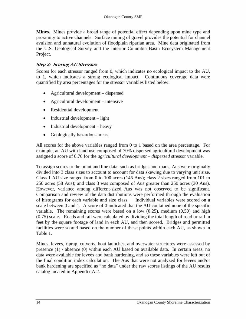
Step 2: Scoring AU Stressors Scores for each stressor ranged from 0, which indicates no ecological impact to the AU, to 1, which indicates a strong ecological impact. Continuous coverage data were quantified by area percentages for the stressor variables listed below:

• Agricultural development – dispersed

• Agricultural development – intensive

• Residential development

• Industrial development – light

• Industrial development – heavy

• Geologically hazardous areas

All scores for the above variables ranged from 0 to 1 based on the area percentage. For example, an AU with land use composed of 70% dispersed agricultural development was assigned a score of 0.70 for the agricultural development – dispersed stressor variable.

To assign scores to the point and line data, such as bridges and roads, Aus were originally divided into 3 class sizes to account to account for data skewing due to varying unit size. Class 1 AU size ranged from 0 to 100 acres (145 Aus); class 2 sizes ranged from 101 to 250 acres (58 Aus); and class 3 was composed of Aus greater than 250 acres (30 Aus). However, variance among different-sized Aus was not observed to be significant. Comparison and review of the data distributions were performed through the evaluation of histograms for each variable and size class. Individual variables were scored on a scale between 0 and 1. A score of 0 indicated that the AU contained none of the specific variable. The remaining scores were based on a low (0.25), medium (0.50) and high (0.75) scale. Roads and rail were calculated by dividing the total length of road or rail in feet by the square footage of land in each AU, and then scored. Bridges and permitted facilities were scored based on the number of these points within each AU, as shown in Table 1.

Mines, levees, riprap, culverts, boat launches, and overwater structures were assessed by presence (1) / absence (0) within each AU based on available data. In certain areas, no data were available for levees and bank hardening, and so these variables were left out of the final condition index calculation. The Aus that were not analyzed for levees and/or bank hardening are specified as “no data” under the raw scores listings of the AU results catalog located in Appendix A.2.


Okanogan County SMP

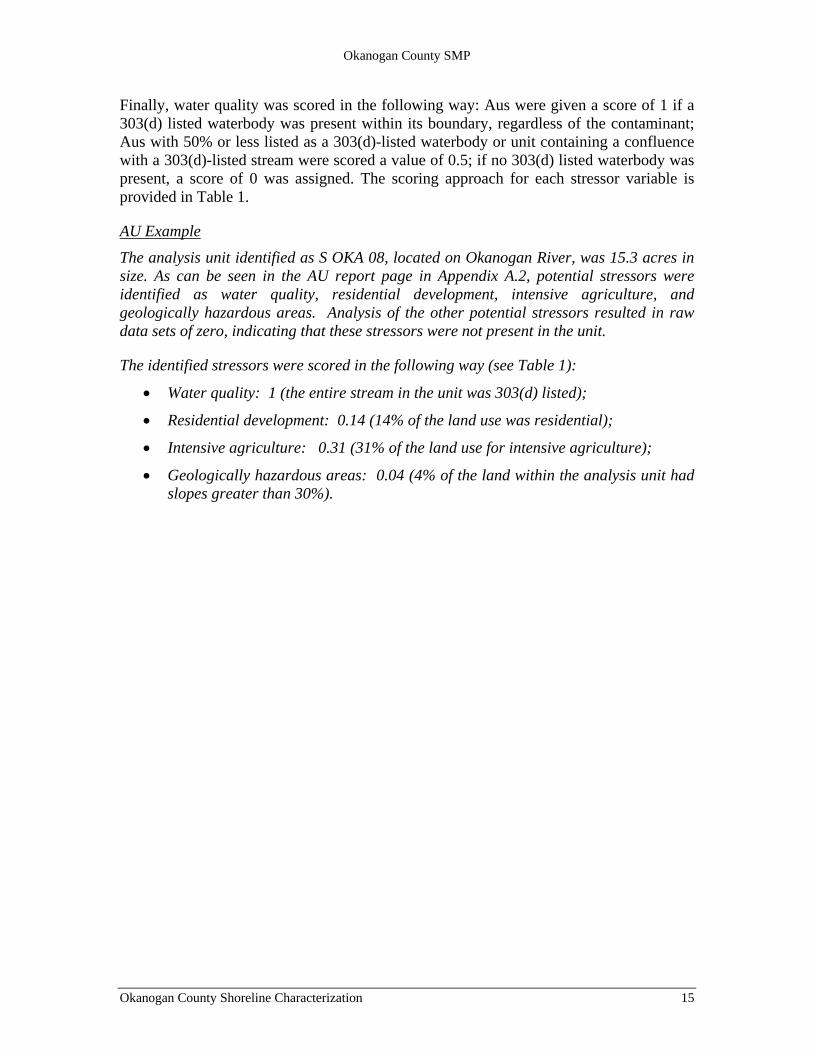
Finally, water quality was scored in the following way: Aus were given a score of 1 if a 303(d) listed waterbody was present within its boundary, regardless of the contaminant; Aus with 50% or less listed as a 303(d)-listed waterbody or unit containing a confluence with a 303(d)-listed stream were scored a value of 0.5; if no 303(d) listed waterbody was present, a score of 0 was assigned. The scoring approach for each stressor variable is provided in Table 1.

AU Example

The analysis unit identified as S OKA 08, located on Okanogan River, was 15.3 acres in size. As can be seen in the AU report page in Appendix A.2, potential stressors were identified as water quality, residential development, intensive agriculture, and geologically hazardous areas. Analysis of the other potential stressors resulted in raw data sets of zero, indicating that these stressors were not present in the unit.

The identified stressors were scored in the following way (see Table 1):

• Water quality: 1 (the entire stream in the unit was 303(d) listed);

• Residential development: 0.14 (14% of the land use was residential);

• Intensive agriculture: 0.31 (31% of the land use for intensive agriculture);

• Geologically hazardous areas: 0.04 (4% of the land within the analysis unit had slopes greater than 30%).


Okanogan County SMP

Table 1: Analysis Unit Stressor Scoring and Weighting

AU Stressor Score Scoring Weight

Agricultural dev-dispersed 0 to 1 Percentage of disperse agricultural land in unit 25

Agricultural dev-Intensive 0 to 1 Percentage of intensive agricultural land in unit 50

Residential dev 0 to 1 Percentage of residential area in unit 75

Industrial dev-light 0 to 1 Percentage of disperse light industrial activity area in unit 50

Industrial dev-heavy 0 to 1 Percentage of disperse heavy industrial activity area in unit 75

Mines 0 No mines 25

1 I or more mines in unit -

Levees 0 No levees 75

1 Has levees in unit -

Riprap 0 No riprap 75

1 Has riprap in unit -

Culverts 0 No culverts in unit 50

1 I or more culverts in unit -

Boat launches 0 No boat launches in unit 25

1 I or more boat launches in unit -

Overwater structures 0 No overwater structures in unit 25

1 I or more overwater structures in unit -

Water quality class 0 No 303(d)-listed waterbodies 75

0.5 50% or less listed as a 303(d)-listed waterbody or unit containing a confluence with a 303(d)-listed stream

1 Entire unit 303(d)-listed

Facilities – Permitting 0.00 No permitted facilities in unit 25

0.25 1 to 5 facilities in unit -

0.50 6 to 10 facilities in unit -

0.75 11 or more in unit -

Bridges 0.00 No bridges in unit 25

0.25 1 bridge in unit -

0.50 Up to 3 bridges in unit -

0.75 4 or more bridges in unit -

Rail 0.00 No rail (Rail evaluated by feet of rail per square footage of land in AU) 75

0.25 up to 0.0005 -

0.50 up to 0.0010 -

0.75 0.0011 or more -

Roads 0.00 No roads (Roads evaluated by feet of road per square footage of land in AU) 75

0.25 up to 0.0005 -

0.50 up to 0.0010 -

0.75 0.0011 or more -


Okanogan County SMP

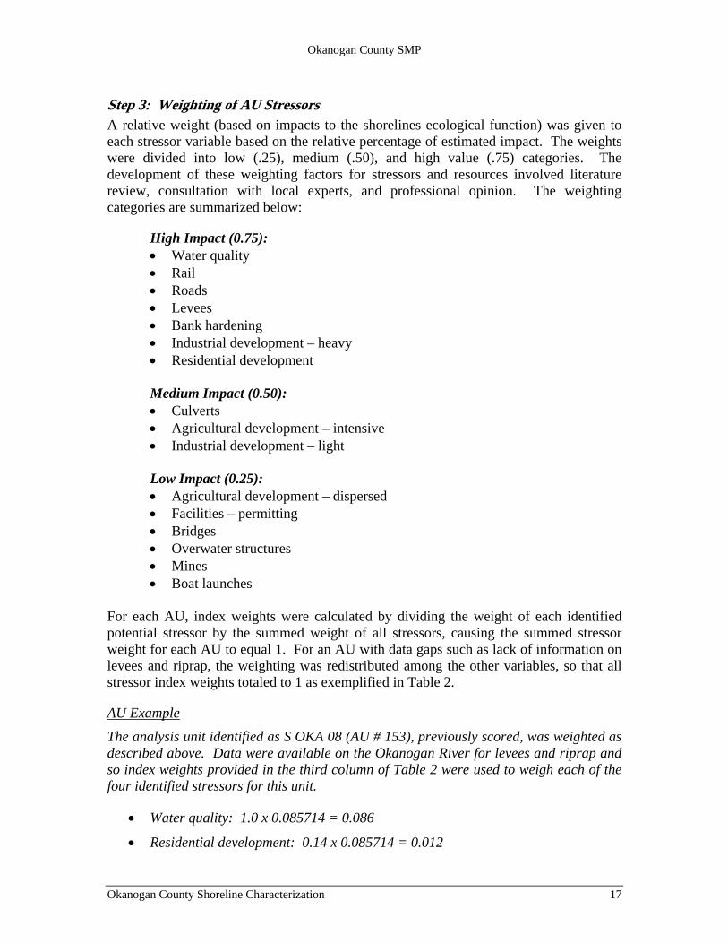
Step 3: Weighting of AU Stressors A relative weight (based on impacts to the shorelines ecological function) was given to each stressor variable based on the relative percentage of estimated impact. The weights were divided into low (.25), medium (.50), and high value (.75) categories. The development of these weighting factors for stressors and resources involved literature review, consultation with local experts, and professional opinion. The weighting categories are summarized below:

High Impact (0.75): • Water quality • Rail • Roads • Levees • Bank hardening • Industrial development – heavy • Residential development

Medium Impact (0.50):

• Culverts • Agricultural development – intensive • Industrial development – light

Low Impact (0.25):

• Agricultural development – dispersed • Facilities – permitting • Bridges • Overwater structures • Mines • Boat launches

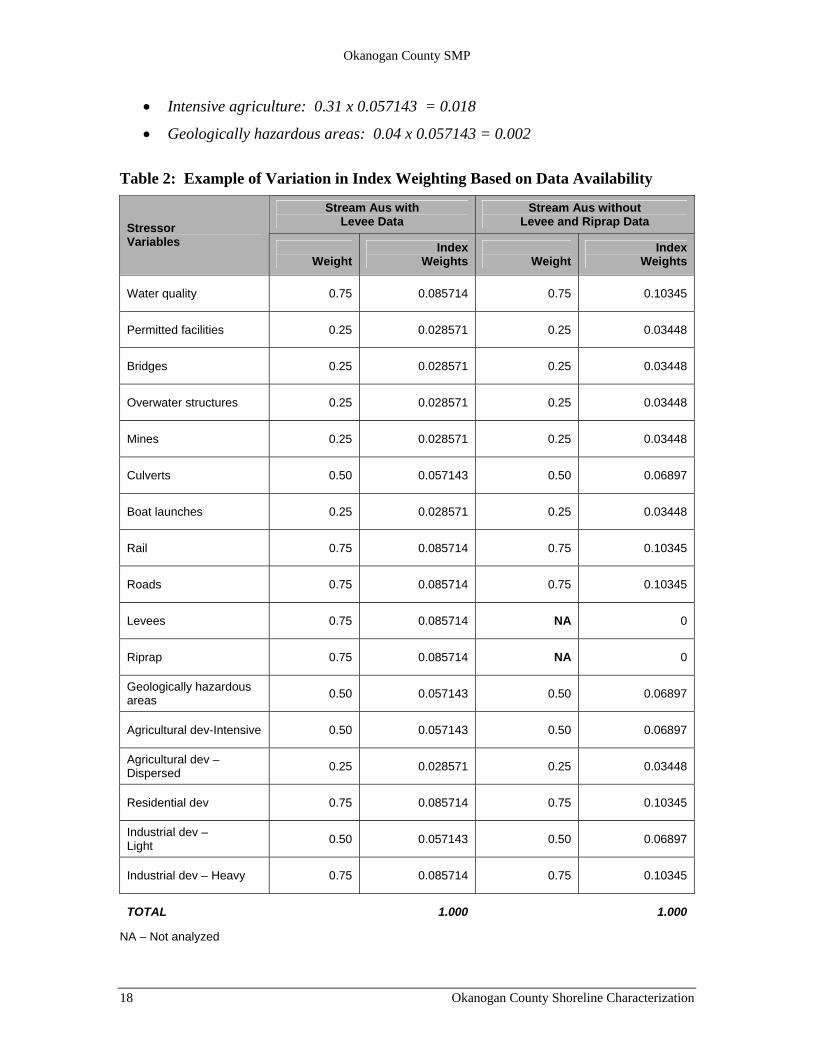
For each AU, index weights were calculated by dividing the weight of each identified potential stressor by the summed weight of all stressors, causing the summed stressor weight for each AU to equal 1. For an AU with data gaps such as lack of information on levees and riprap, the weighting was redistributed among the other variables, so that all stressor index weights totaled to 1 as exemplified in Table 2.

AU Example

The analysis unit identified as S OKA 08 (AU # 153), previously scored, was weighted as described above. Data were available on the Okanogan River for levees and riprap and so index weights provided in the third column of Table 2 were used to weigh each of the four identified stressors for this unit.

• Water quality: 1.0 x 0.085714 = 0.086

• Residential development: 0.14 x 0.085714 = 0.012


Okanogan County SMP

• Intensive agriculture: 0.31 x 0.057143 = 0.018

• Geologically hazardous areas: 0.04 x 0.057143 = 0.002

Table 2: Example of Variation in Index Weighting Based on Data Availability

Stream Aus with Levee Data

Stream Aus without Levee and Riprap Data Stressor

Variables Weight

Index Weights

Weight

Index Weights

Water quality 0.75 0.085714 0.75 0.10345

Permitted facilities 0.25 0.028571 0.25 0.03448

Bridges 0.25 0.028571 0.25 0.03448

Overwater structures 0.25 0.028571 0.25 0.03448

Mines 0.25 0.028571 0.25 0.03448

Culverts 0.50 0.057143 0.50 0.06897

Boat launches 0.25 0.028571 0.25 0.03448

Rail 0.75 0.085714 0.75 0.10345

Roads 0.75 0.085714 0.75 0.10345

Levees 0.75 0.085714 NA 0

Riprap 0.75 0.085714 NA 0

Geologically hazardous areas 0.50 0.057143 0.50 0.06897

Agricultural dev-Intensive 0.50 0.057143 0.50 0.06897

Agricultural dev – Dispersed 0.25 0.028571 0.25 0.03448

Residential dev 0.75 0.085714 0.75 0.10345

Industrial dev – Light 0.50 0.057143 0.50 0.06897

Industrial dev – Heavy 0.75 0.085714 0.75 0.10345

TOTAL 1.000 1.000

NA – Not analyzed


Okanogan County SMP

Step 4: Calculation of AU Condition Index For each AU, the stressor scores were multiplied by the index weight values and added. The result was a stressor index value for each AU that ranged from 0 to 1. The condition index value for each AU was then calculated by subtracting the combined stressor score from 1. This inverted the ranking of sites from higher values signifying greater impacts to higher values signifying greater overall condition health. In this way, higher condition values indicate a less altered condition, while lower condition values indicate a more altered condition.

AU Example

The analysis unit identified as S OKA 08 (AU # 153), previously scored and weighted, had a stressor index value calculated by adding the products of the scores and index weights: 0.086 (water quality) + 0.012 (residential development) + 0.018 (intensive agriculture) + 0.002 (geologically hazardous areas) = 0.118. The condition index value was calculated by subtracting the stressor index value from 1: 1 – 0.118 =0.88.

3.2.4 Aggregate Resource Index

Step 1: Identification of AU Resources The resource data identified for use in this analysis were chosen for their indication of the relative ecological function of the shoreline. County wide coverage was the basis for selecting variables and datasets to the extent possible. These data were the most comprehensive public data available at the time of analysis. Individual variables are described below.

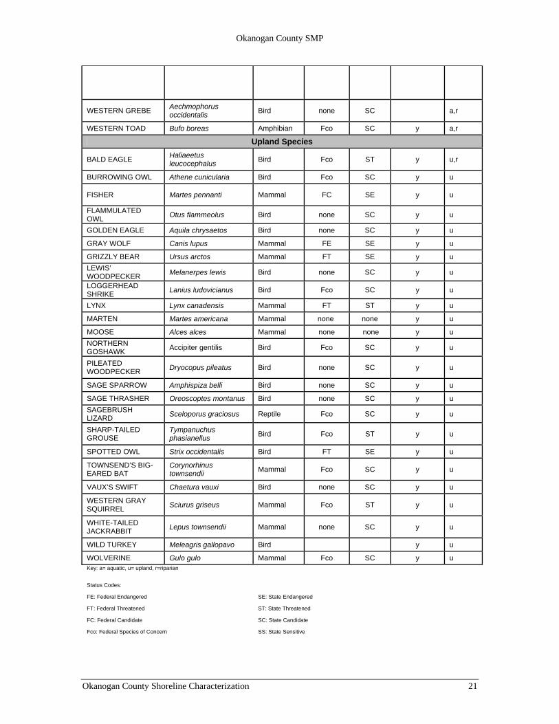
Species. Species of Concern in Washington, as identified by the Washington Department of Fish and Wildlife (WDFG), include all State Endangered, Threatened, Sensitive, and Candidate species as well as Federal Endangered, Threatened, and Candidate species. Additionally, Priority Species listed by WDFW includes the above species as well as game species and organisms crucial to tribal cultural values. Some species distribution data could not be obtained, due either to data gaps or absence of the species within the SMP study area. The number of distributions of these aquatic, riparian, and upland species were totaled for each AU. Certain species were assigned to more than one habitat. Data for the species distributions were obtained from NOAA Fisheries, the Washington GAP Project created by Washington Cooperative Fish and Wildlife Research Unit, the StreamNet Project, and the Priority and Species Database and Wildlife Heritage Database created by WDFG. A complete list of species used in this analysis is provided in Table 3.


Okanogan County SMP

Table 3: Species Included in AU Resource Scoring

Common Name Scientific Name Animal Type

Federal Status

State Status

WA Priority Sp.

Status Habitat

Aquatic Species AMERICAN WHITE PELICAN

Pelecanus erythrorhynchos Bird none SE y a

BARROW’S GOLDENEYE Bucephala islandica Bird None none y a,r

BULL TROUT Salvelinus confluentus Fish FT SC y a

COLUMBIA SPOTTED FROG Rana luteiventris Amphibian none SC y a,r

COMMON LOON Gavia immer Bird none SS y a,r

GIANT COLUMBIA RIVER LIMPET Fisherola nuttalli Mollusk none SC y a

GREAT BLUE HERON Ardea herodias Bird None none y a,r

GREAT COLUMBIA SPIRE SNAIL Fluminicola columbiana Mollusk Fco SC y a

HARLEQUIN DUCK Histrionicus histrionicus Bird None none y a,r LARGEMOUTH BASS Micropterus salmoides Fish None none y a

OREGON SPOTTED FROG Rana pretiosa Amphibian FC SE y a,r

PYGMY WHITEFISH Prosopium coulteri Fish Fco SS y a

SMALLMOUTH BASS Micropterus dolomieui Fish y a

SOCKEYE SALMON OR KOKANEE Oncorhynchus nerka Fish FE SC y a

UMATILLA DACE Rhinichthys umatilla Fish none SC y a

WALLEYE Stizostedion vitreum Fish none none y a

WESTERN GREBE Aechmophorus occidentalis Bird none SC y a,r

WESTERN TOAD Bufo boreas Amphibian Fco SC y a,r

WESTSLOPE CUTTHROAT

Oncorhynchus clarki lewisi Fish none none y a

WHITE STURGEON Acipenser transmontanus Fish None none y a

Riparian Species

BALD EAGLE Haliaeetus leucocephalus Bird Fco ST y u,r

BARROW’S GOLDENEYE Bucephala islandica Bird None none y a,r

COLUMBIA SPOTTED FROG Rana luteiventris Amphibian none SC y a,r

COMMON LOON Gavia immer Bird none SS y a,r GREAT BLUE HERON Ardea herodias Bird none none y a,r

HARLEQUIN DUCK Histrionicus histrionicus Bird none none y a,r

OREGON SPOTTED FROG Rana pretiosa Amphibian FC SE y a,r


Okanogan County SMP

WESTERN GREBE Aechmophorus occidentalis Bird none SC a,r

WESTERN TOAD Bufo boreas Amphibian Fco SC y a,r

Upland Species

BALD EAGLE Haliaeetus leucocephalus Bird Fco ST y u,r

BURROWING OWL Athene cunicularia Bird Fco SC y u

FISHER Martes pennanti Mammal FC SE y u

FLAMMULATED OWL Otus flammeolus Bird none SC y u

GOLDEN EAGLE Aquila chrysaetos Bird none SC y u

GRAY WOLF Canis lupus Mammal FE SE y u

GRIZZLY BEAR Ursus arctos Mammal FT SE y u LEWIS’ WOODPECKER Melanerpes lewis Bird none SC y u

LOGGERHEAD SHRIKE Lanius ludovicianus Bird Fco SC y u

LYNX Lynx canadensis Mammal FT ST y u

MARTEN Martes americana Mammal none none y u

MOOSE Alces alces Mammal none none y u NORTHERN GOSHAWK Accipiter gentilis Bird Fco SC y u

PILEATED WOODPECKER Dryocopus pileatus Bird none SC y u

SAGE SPARROW Amphispiza belli Bird none SC y u

SAGE THRASHER Oreoscoptes montanus Bird none SC y u SAGEBRUSH LIZARD Sceloporus graciosus Reptile Fco SC y u

SHARP-TAILED GROUSE

Tympanuchus phasianellus Bird Fco ST y u

SPOTTED OWL Strix occidentalis Bird FT SE y u

TOWNSEND’S BIG-EARED BAT

Corynorhinus townsendii Mammal Fco SC y u

VAUX’S SWIFT Chaetura vauxi Bird none SC y u

WESTERN GRAY SQUIRREL Sciurus griseus Mammal Fco ST y u

WHITE-TAILED JACKRABBIT Lepus townsendii Mammal none SC y u

WILD TURKEY Meleagris gallopavo Bird y u

WOLVERINE Gulo gulo Mammal Fco SC y u Key: a= aquatic, u= upland, r=riparian

Status Codes:

FE: Federal Endangered SE: State Endangered

FT: Federal Threatened ST: State Threatened

FC: Federal Candidate SC: State Candidate

Fco: Federal Species of Concern SS: State Sensitive


Okanogan County SMP

Salmon Spawning and Rearing Habitat. It has been argued that biological diversity, in relation to large-scale ecological processes versus just a mix of species, should focus on keystone species (focal) or those essential for ecosystem resilience. Salmonids have been used as focal species in several local watershed planning documents for the area (NPCC, 2004a; NPCC, 2004b). Therefore, for this shoreline characterization analysis, Aus containing salmonid habitat represent vital areas.

Habitat loss and change are among the major factors determining the current status of salmonid populations. Salmonids depend on diverse habitats with connections among those habitats for their life history cycle from rearing to spawning. Data for this analysis were provided the National Oceanic and Atmospheric Administration (NOAA), Streamnet, and WDFW. Lake Aus were not analyzed for this variable.

ESA Salmon Critical Habitat. NOAA fisheries Northwest Region critical habitat designations include habitat for Chinook salmon and rainbow trout/steelhead species within Okanogan County. These are specific areas that have been found to be critical to conservation of salmonid species, and include not only spawning and rearing habitat but also important migration habitat. Loss of this habitat reduces the diversity in salmon and steelhead life histories, which influences the ability of these fish to adapt to natural and man-made change. Critical habitat designation data were provided by NOAA. Lake Aus were not analyzed for this variable.

Riparian Vegetation. Riparian habitat is especially important in the western United States due to the presence of water and vegetation, typically surrounded by harsher, drier, less productive environments (Chaney et al., 1990). Riparian vegetation provides several benefits to shorelines. Tree roots uptake nutrients along with other pollutants that ordinate from the land and are stored in leaves, limbs, and roots. Riparian vegetation stabilizes the soil along shorelines, reduces the risk of flooding, and provides large woody debris to the aquatic environment. The canopy provides shade that keeps water cool and retains more dissolved oxygen both of which are needed for many of the life stages of aquatic species. The score was based on the percentage of riparian vegetation within each AU and was calculated from the U.S. Geological Survey (USGS) Land Cover GIS data layer.

Wetlands. Wetlands are essential in assisting in flood control as they can store water and also filter pollutants and retain sediments. Many species depend on wetlands for some part of their life cycle (breeding, nesting, feeding, shelter). Data were obtained from the National Wetland Inventory which provides information on the characteristics, extent, and status of US wetlands and deepwater habitats. The National Wetland Inventory created by WDFG was accessed to provide the location and extent of wetlands in Okanogan County.

Potential Migration Zones. The area where the stream channel is most likely to move across the floodplain, over time, has the ability to reduce flood hazards and create habitat for a wide range of species. This area is commonly referred to as the channel migration zone but, for this analysis this zone is referred to as the Potential Migration Zone (PMZ). The PMZ layer was created based on interpretations from a low-resolution digital


Okanogan County SMP

elevation models (DEM) and general published geologic maps. ENTRIX or its employees are not responsible for specific delineation boundaries in any way unless and until a thorough analysis that includes higher resolution mapping, photogrammetric interpretation, and field calibration is accomplished. Provision of such a rigorous analysis for delineation of lateral channel movement was beyond the scope and budget of this project. The PMZ is provided as a general guide to channel conditions based on available information and is not intended for use in other jurisdictional delineations. This PMZ can be considered some index of the potential for a channel to migrate, but cannot be directly interpreted as the defined probability of lateral channel movements. Lake Aus were not analyzed for this variable.

Step 2: Scoring of AU Resources Scores for resources range from 0, which estimates an absence of identified resources, to 1, which estimates a strong presence of identified resources (Table 4). In this way, higher scores indicate a relatively higher value of resources in an analysis unit, while lower scores indicate a lower value of resources.

Continuous coverage data were quantified by area percentages for the stressor variables listed below:

• Wetlands

• Riparian vegetation

• Potential migration zone

All scores for the above variables ranged from 0 to 1 based on the area percentage. For example, an AU composed of 30% riparian vegetation was assigned a score of 0.30 for the riparian vegetation resource variable.

To assign scores to the aquatic, riparian, and upland species distributions data, Aus were originally divided into 3 class sizes to account to account for data skewing due to varying unit size as described above. However, variance among different-sized Aus were not observed to be significant, and so class sizes were eliminated from the analysis. Individual variables were scored on a scale between 0 and 1. The scores were based on a low (0.25), medium (0.50) and high (0.75) number of species found within each AU as described in Table 5.

Finally, due to the nature of the data used in this analysis, the following variables were assessed based on presence (1)/ absence (0) within each AU:

• Salmon spawning / rearing habitat

• NOAA critical habitat


Okanogan County SMP

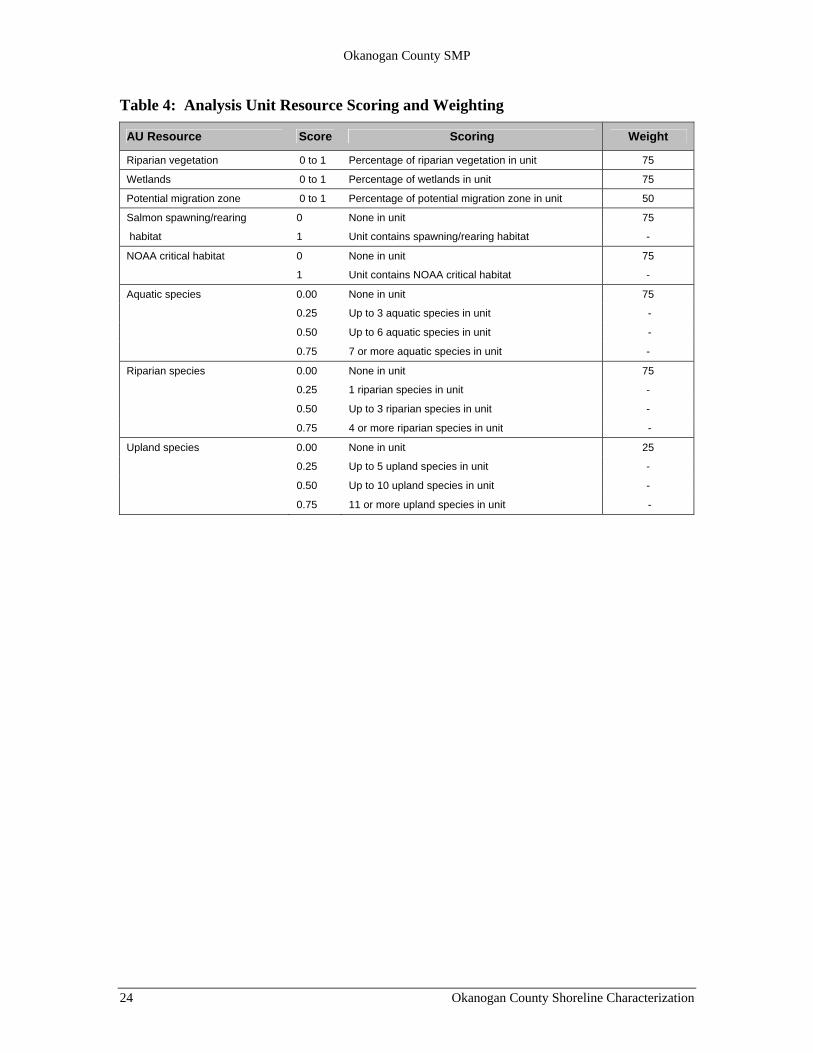
Table 4: Analysis Unit Resource Scoring and Weighting

AU Resource Score Scoring Weight

Riparian vegetation 0 to 1 Percentage of riparian vegetation in unit 75

Wetlands 0 to 1 Percentage of wetlands in unit 75

Potential migration zone 0 to 1 Percentage of potential migration zone in unit 50

Salmon spawning/rearing 0 None in unit 75

habitat 1 Unit contains spawning/rearing habitat -

NOAA critical habitat 0 None in unit 75

1 Unit contains NOAA critical habitat -

Aquatic species 0.00 None in unit 75

0.25 Up to 3 aquatic species in unit -

0.50 Up to 6 aquatic species in unit -

0.75 7 or more aquatic species in unit -

Riparian species 0.00 None in unit 75

0.25 1 riparian species in unit -

0.50 Up to 3 riparian species in unit -

0.75 4 or more riparian species in unit -

Upland species 0.00 None in unit 25

0.25 Up to 5 upland species in unit -

0.50 Up to 10 upland species in unit -

0.75 11 or more upland species in unit -


Okanogan County SMP

AU Example

As seen before, the analysis unit identified as S OKA 08 (AU #153), located on Okanogan River was 15.3 acres in size. Identified potential resources were identified as aquatic, riparian, and upland species, salmon spawning and rearing habitat, NOAA critical habitat, riparian vegetation, wetlands, and potential migration zone. The identified resources were scored in the following way (see Table 5):

• Aquatic species: 0.75 (data on 10 species distributions in unit );

• Riparian species: 0.50 (data on 3 species distributions in unit);

• Upland species: 0.75 (data on 15 species distributions in unit)

• Salmon spawning/rearing habitat: 1.0 (present in unit);

• NOAA critical habitat: 1.0 (present in unit);

• Riparian vegetation: 0.30 (30% of the land within unit had riparian vegetation);

• Wetlands: 0.074 (7.4% of the land within unit was composed of wetlands);

• Potential migration zone: 1.0 (100% of the AU within the potential migration zone)

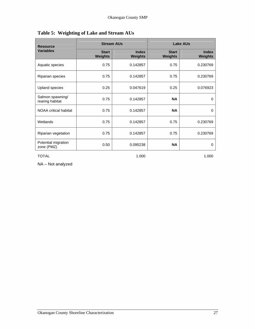
Step 3: Weighting of AU Resources A relative weight (based on the value of each resource to shoreline ecological function) was given to each resource variable. The score was multiplied by this weighting factor based on the relative percentage of estimated value. The weights were divided into low (.25), medium (.50), and high value (.75) categories. The development of these weighting factors for resources involved literature review, consultation with local experts, and professional opinion. The weighting categories are summarized below:

High Resource Value (0.75): • Aquatic species • Riparian species • Salmon spawning / rearing habitat • NOAA critical habitat • Wetlands • Riparian vegetation

Medium Resource Value (0.50):

• Potential migration zones Low Resource Value (0.25):

• Upland species Resource index weights were calculated by dividing the weight of each analyzed resource by the summed weight of all analyzed resources in each unit, causing the summed resource weights for each AU to equal 1. The resource scores were then multiplied by


Okanogan County SMP

the index weight values. Lake and stream Aus were analyzed for a different number of total resource variables due to the applicability of these variables. Lake Aus were not analyzed for salmon spawning and rearing habitat, NOAA critical habitat, or potential migration zones. Examples of index weighting for stream Aus verses lake Aus is provided in Table 5.

AU Example

The analysis unit identified as S OKA 08 (AU # 153), previously scored, was weighted as described above. This AU was located on a stream and so index weights provided in the third column of Table 6 were used to weigh each of the identified resource variables for this unit.

• Aquatic species: 0.75 x 0.142857 = 0.11;

• Riparian species: 0.50 x 0.142857 = 0.071;

• Upland species: 0.75 x 0.047619 = 0.036;

• Salmon spawning/rearing habitat: 1.0 x 0.142857 = 0.14;

• NOAA critical habitat: 1.0 x 0.142857 = 0.14;

• Riparian vegetation: 0.30 x 0.142857 = 0.043;

• Wetlands: 0.074 x 0.142857 = 0.011;

• Potential migration zone: 1.0 x 0.095238 = 0.095.

Step 4: Calculation of AU Resource Index The combined resource score for each AU was calculated by adding the individual weighted resource scores. The result, a resource index score for each AU that ranged from 0 to 1, was used to assess the relative ecological health of each shoreline unit.

AU Example

The analysis unit identified as S OKA 08 (AU # 153), previously scored and weighted, had a resource index value calculated by adding the products of the scores and index weights: 0.11 (aquatic species) + 0.071 (riparian species) + 0.036 (upland species) + 0.14 (salmon spawning/rearing habitat) + 0.14 (NOAA critical habitat) + 0.043 (riparian vegetation) + 0.011 (wetlands) + 0.095 (potential migration zone) = 0.65.


Okanogan County SMP

Table 5: Weighting of Lake and Stream AUs

Stream AUs Lake AUs Resource Variables Start

Weights Index

Weights Start

Weights Index

Weights

Aquatic species 0.75 0.142857 0.75 0.230769

Riparian species 0.75 0.142857 0.75 0.230769

Upland species 0.25 0.047619 0.25 0.076923

Salmon spawning/ rearing habitat 0.75 0.142857 NA 0

NOAA critical habitat 0.75 0.142857 NA 0

Wetlands 0.75 0.142857 0.75 0.230769

Riparian vegetation 0.75 0.142857 0.75 0.230769

Potential migration zone (PMZ) 0.50 0.095238 NA 0

TOTAL 1.000 1.000

NA – Not analyzed


Okanogan County SMP

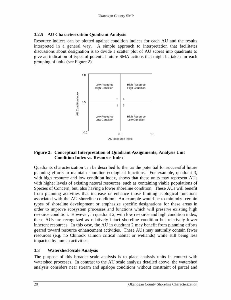
3.2.5 AU Characterization Quadrant Analysis Resource indices can be plotted against condition indices for each AU and the results interpreted in a general way. A simple approach to interpretation that facilitates discussions about designation is to divide a scatter plot of AU scores into quadrants to give an indication of types of potential future SMA actions that might be taken for each grouping of units (see Figure 2).

1.0

1.00.0 0.5

0.5

High Resource Low Condition

Low Resource Low Condition

Low ResourceHigh Condition

High Resource High Condition

AU Resource Index

AU C

ondi

tion

Inde

x

1

4

3

2

Figure 2: Conceptual Interpretation of Quadrant Assignments; Analysis Unit Condition Index vs. Resource Index

Quadrants characterization can be described further as the potential for successful future planning efforts to maintain shoreline ecological functions. For example, quadrant 3, with high resource and low condition index, shows that these units may represent AUs with higher levels of existing natural resources, such as containing viable populations of Species of Concern, but, also having a lower shoreline condition. These AUs will benefit from planning activities that increase or enhance those limiting ecological functions associated with the AU shoreline condition. An example would be to minimize certain types of shoreline development or emphasize specific designations for these areas in order to improve ecosystem processes and functions which will preserve existing high resource condition. However, in quadrant 2, with low resource and high condition index, these AUs are recognized as relatively intact shoreline condition but relatively lower inherent resources. In this case, the AU in quadrant 2 may benefit from planning efforts geared toward resource enhancement activities. These AUs may naturally contain fewer resources (e.g. no Chinook salmon critical habitat or wetlands) while still being less impacted by human activities.

3.3 Watershed-Scale Analysis The purpose of this broader scale analysis is to place analysis units in context with watershed processes. In contrast to the AU scale analysis detailed above, the watershed analysis considers near stream and upslope conditions without constraint of parcel and


Okanogan County SMP

ownership inclusion in the shoreline management jurisdiction. The primary value of watershed scale analysis is the identification of AUs and stressor functions that might be used to identify restoration actions as well as to evaluate the relative intactness of AUs within each watershed. This analysis will be a part of the final report.

The method to highlight watershed key processes and describe the effects of land use on those key processes will be modified from Ecology’s 2005 document, available at: http://www.ecy.wa.gov/biblio/0506027.html. The goal is to identity and map areas important to sustain shoreline functions and to determine degree of alteration to key processes. The following is a list of the three key watershed process and likely indicators that will be used to evaluate them:

• Sediment supply and erosion - soil erodibility index, dams, mass wasting areas;

• Riparian inputs (heat/light) - riparian vegetation, fire history;

• Hydrology - precipitation, recharge areas, soil permeability (PCMZ).

Indicators of alteration that may be used are, roads 100’ of streams, dams, urban land cover, non-forest cover 100’ of streams, agriculture cover, urban cover on high soil permeability, and impervious surfaces. The indictors of key processes and indicators of alteration will be overlaid spatially in order to highlight minimally altered areas and impaired areas within each watershed.

3.3.1 Watershed Boundaries In general terms, watersheds are an area of land that drains water, sediment and dissolved materials to a common receiving body or outlet. Watersheds vary from the largest river basins to just acres or less in size. Watershed delineations have been completed for the Methow and Okanogan Subbasin plans and limiting factor analysis (ENTRIX and Golder 2002, MWG et al. 1995; NPCC 2004a, NPCC 2004b). However, these were created under a different set of goals where, for example, the project focused on focal salmonid distributions. This watershed analysis used boundaries were meaningful descriptions of upslope factors (vegetation, wetlands, land use etc.) interact to describe the AU shoreline zone. This characterization framework used best professional judgment in defining watersheds.

Watershed boundaries were primarily determined by utilizing the USGS 5th Field Hydrologic Unit (HUC 10) which represent major watershed delineations (i.e., large tributaries and HUC 12. The watersheds evaluated within Okanogan County are:

Upper Methow Watershed Mazama Watershed Lower Chewuch Watershed Middle Methow River Watershed Beaver Watershed Twisp Watershed Lower Methow River Watershed


http://www.ecy.wa.gov/biblio/0506027.html

Okanogan County SMP

Upper Columbia/Swamp Creek Watershed Sinlahekin Watershed Lower Similkameen River Watershed Upper Okanogan River Watershed Okanogan River watershed Bonaparte Watershed Okanogan River/ Omak Watershed Salmon Watershed Lower Okanogan Watershed Myers Watershed Toroda Watershed West Fork Sanpoil Watershed


4 CHARACTERIZATION RESULTS 4.1 Introduction The results of site-scale analyses of the shoreline area of Okanogan County are presented in the AU characterization summary reports located in Technical Appendix A.2. Maps depicting the relative locations of each AU within Okanogan County are provided in the Map Portfolio (Appendix A.4). Tables summarizing the lakes and streams evaluated in this characterization are located in Technical Appendix A.3, Tables 1 and 2. Tables providing a complete catalog list of all AUs for lakes and streams that serve as a roadmap for the AU characterization results catalog can be found in Technical Appendix A.3, Tables 3 and 4. Appendix A.3, Table 5 lists the descriptive statistics for each analysis variable. Appendix A.3 Table 6 provides a list of data sources used in this analysis.

4.2 AU Characterization Results Catalog Each of the 233 analysis units have an individual one-page report that identifies information unique to each AU such as AU number, AU code, latitude and longitude of each AU center point, waterbody name, and watershed. Along with this identifying information, both raw and final scores are presented for each variable, the aggregate condition and resource indices for each AU, and quadrant results. Maps of Watersheds and AUs are included as a companion to the AU catalog (Map Portfolio).

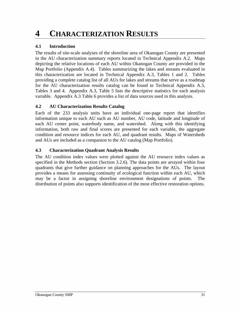
4.3 Characterization Quadrant Analysis Results The AU condition index values were plotted against the AU resource index values as specified in the Methods section (Section 3.2.6). The data points are arrayed within four quadrants that give further guidance on planning approaches for the AUs. The layout provides a means for assessing continuity of ecological function within each AU, which may be a factor in assigning shoreline environment designations of points. The distribution of points also supports identification of the most effective restoration options.


Okanogan County SMP

0.00

0.20

0.40

0.60

0.80

1.00

0.00 0.50 1.00

Resource Index

Cond

ition

Inde

x

Figure 3: Plot of AU Condition and Resource Indices, Okanogan County, WA

(n=233)

A scatter plot of AU condition and resource indices is provided in Figure 3 and 4. Condition indices of all AUs ranged from 0.53 to 0.97. Resource indices for all AUs ranged from 0.21 to 0.86. As can be seen in Figure 3, this caused all of the values to be located in the upper half of the scatter plot.

Figure 5 shows the distribution of AUs within each quadrant. Quadrant results by AU are located in Technical Appendix A.3, Table 4.


Okanogan County SMP

AU Quadrant Plot May, 2008

0.50

0.83

0.00 0.55

Resource Index

Con

ditio

n In

dex

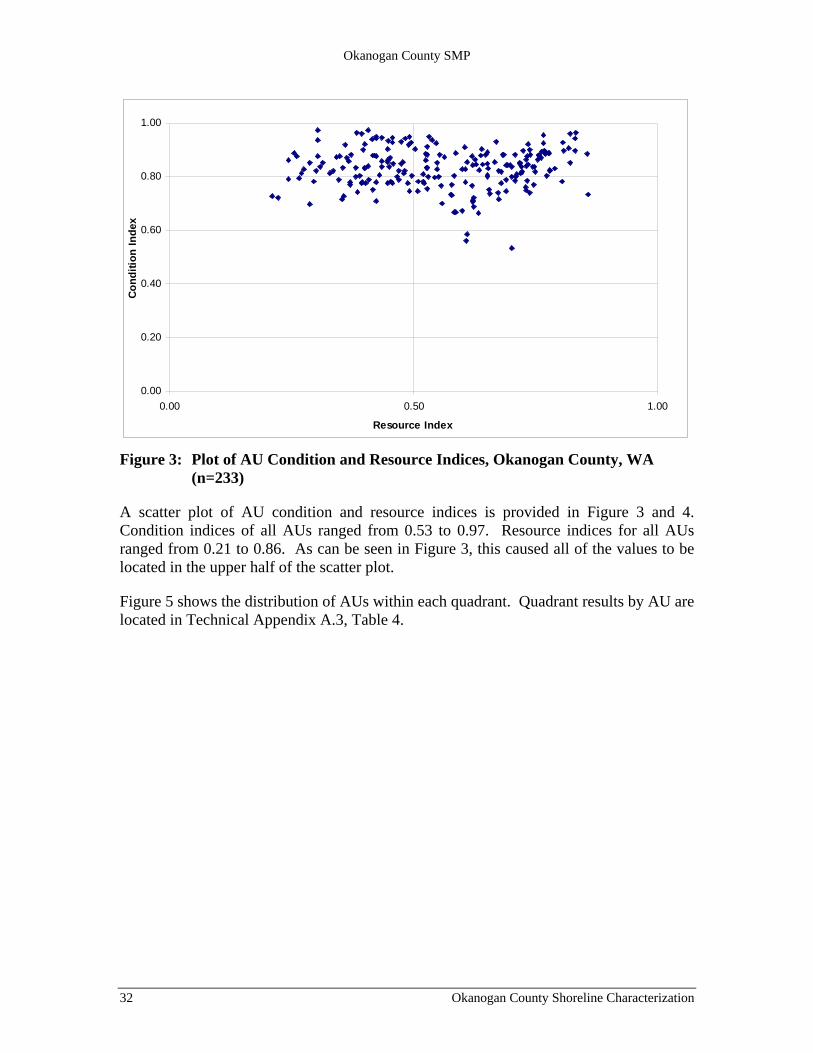
Figure 4: Modified AU condition and resource Indices’ Plot Showing Approximate

Location of Quadrant Boundaries for Characterization Results

The total numbers of AUs within each quadrant are the following: 1. Low Condition , Low Resource (lower left quadrant) – 43 AUs

2. High Condition, Low Resource (upper left quadrant) – 56 AUs

3. Low Condition, High Resource (lower right quadrant) – 51 AUs

4. High Condition, High Resource (upper right quadrant) – 83 AUs

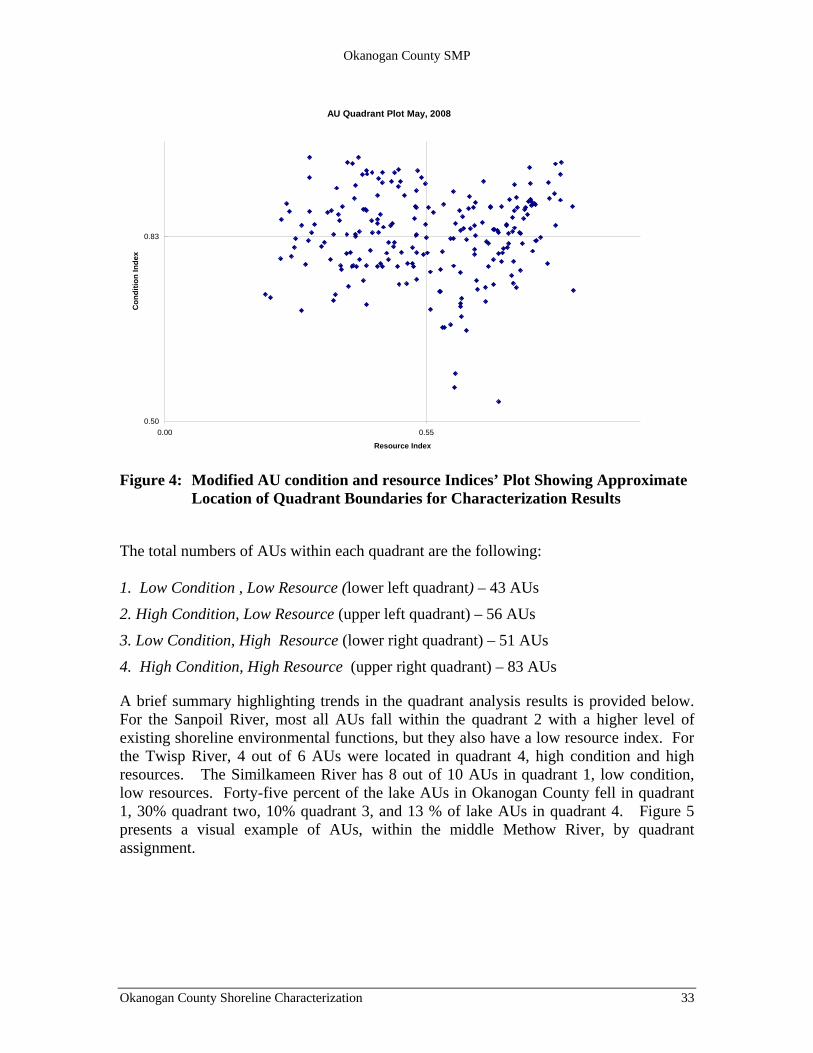
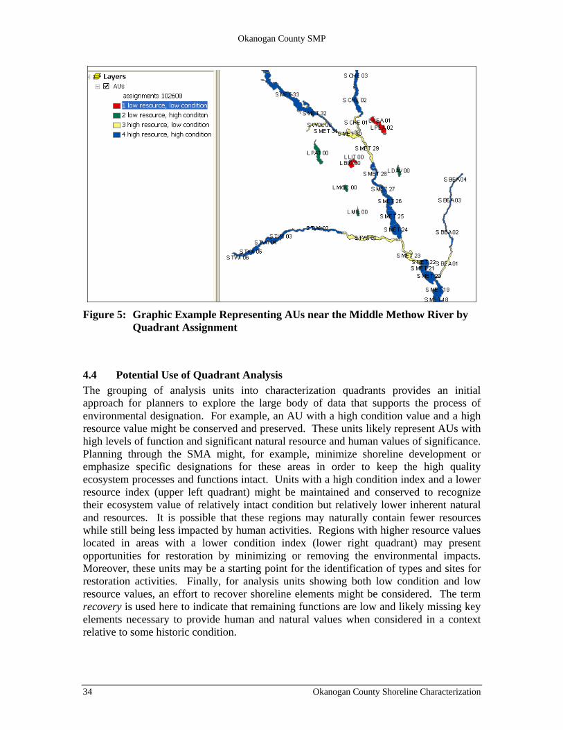
A brief summary highlighting trends in the quadrant analysis results is provided below. For the Sanpoil River, most all AUs fall within the quadrant 2 with a higher level of existing shoreline environmental functions, but they also have a low resource index. For the Twisp River, 4 out of 6 AUs were located in quadrant 4, high condition and high resources. The Similkameen River has 8 out of 10 AUs in quadrant 1, low condition, low resources. Forty-five percent of the lake AUs in Okanogan County fell in quadrant 1, 30% quadrant two, 10% quadrant 3, and 13 % of lake AUs in quadrant 4. Figure 5 presents a visual example of AUs, within the middle Methow River, by quadrant assignment.


Okanogan County SMP

Figure 5: Graphic Example Representing AUs near the Middle Methow River by

Quadrant Assignment

4.4 Potential Use of Quadrant Analysis The grouping of analysis units into characterization quadrants provides an initial approach for planners to explore the large body of data that supports the process of environmental designation. For example, an AU with a high condition value and a high resource value might be conserved and preserved. These units likely represent AUs with high levels of function and significant natural resource and human values of significance. Planning through the SMA might, for example, minimize shoreline development or emphasize specific designations for these areas in order to keep the high quality ecosystem processes and functions intact. Units with a high condition index and a lower resource index (upper left quadrant) might be maintained and conserved to recognize their ecosystem value of relatively intact condition but relatively lower inherent natural and resources. It is possible that these regions may naturally contain fewer resources while still being less impacted by human activities. Regions with higher resource values located in areas with a lower condition index (lower right quadrant) may present opportunities for restoration by minimizing or removing the environmental impacts. Moreover, these units may be a starting point for the identification of types and sites for restoration activities. Finally, for analysis units showing both low condition and low resource values, an effort to recover shoreline elements might be considered. The term recovery is used here to indicate that remaining functions are low and likely missing key elements necessary to provide human and natural values when considered in a context relative to some historic condition.


Okanogan County SMP

4.5 Summary The methodology developed by ENTRIX for characterizing shoreline functions in Okanogan County resulted in the identification of 233 analysis units. These analysis units are distributed across nineteen watersheds. Analyses of characterization results are focused on the presentation and grouping of results by watershed and by descriptive statistical and narrative treatments to assist subsequent planning efforts. A complete catalog of analysis units and attributes for Okanogan County is provided as appendices.


5 CONTINUED SCIENCE SUPPORT FOR SMP UPDATE

5.1 Environmental Designation Determination The data provided in the AU characterization reports will be used as a road map to identify appropriate environmental designations of each reach of shoreline within the County. The ENTRIX science team will coordinate with the planning team to preserve the ecological function of the shoreline area and ensure that no net loss of ecological function occurs.

5.2 Cumulative Effects The cumulative effects analysis will address the effects of all reasonably foreseeable future development on the Okanogan shoreline area. The overall purpose for cumulative impact analysis is to assess the commonly occurring and foreseeable impacts of development that would be allowed and determine whether the net effect of shoreline planning will be to address legislative intent by preventing net loss of shoreline ecological functions and other beneficial uses.

5.3 Restoration Plan The characterization of AU sites suggests shorelines that might be considered as sites for restoration efforts. These opportunities will be explored in the final SMP document.


6 REFERENCES Ashley, P. R. and S. H. Stovall. 2004. Draft Columbia Cascade Ecoprovince Wildlife

Assessment. Unpublished report. Available at Washington Department of Fish and Wildlife office, Spokane, WA. 553 pp.

Angermeier, P.L., A.P. Wheeler, and A.E. Rosenberger. 2004. Fisheries 29:19-29. Brunke, M., and T. Gonser. 1997. The ecological significance of exchange processes

between rivers and groundwater. Freshwater Biology 37:1-33. Chaney, E.; Elmore, W.; and Platts, W. S. 1990. Livestock Grazing on Western Riparian

Areas. United States Environmental Protection Agency ENTRIX, Inc. and Golder Associates, 2002. Salmon and steelhead habitat limiting

factors assessment wria 49: Okanogan watershed. Prepared for : Colville Confederated Tribes and Washington State Conservation Commission.

Evans et al. 2006. Lower Columbia River Restoration Prioritization Framework.

Prepared by Battelle memorial Institute for the Lower Columbia River Estuary Partnership, Richland, Washington.

Findlay, S. 1995. importance of surface-subsurface exchange in stream ecosystems: the

hyporheic zone. Limnol. Oceanogr,. 40(1): 159-164. Fischenich, J.C. 2003. Effects of riprap on riverine and riparian ecosystems. ERDC/EL

TR-03-4, U.S. Army Engineer Research and Development Center, Vicksburg, MS.

IBIS (Interactive Biodiversity Information System). 2003. A wildlife information database established and maintained by the Northwest Habitat Institute. Corvallis, OR. Interior Columbia Basin Ecosystem Management Project (ICBEMP), 1995. Mining

Claim Density – Washington. Available at: http://www.icbemp.gov/ [Accessed 1/2008]

Johnson, D. H. and T. A. O'Neil. 2001. Wildlife-Habitat Relationships in Oregon and

Washington. Oregon State University Press. Leopold, L.B. 1994. A view of the river. Harvard University Press. pp.297. Mitsch, W.J., & J.G. Gosselink , Wetlands, third edition. 2000. John Wiley and Sons,

Canada


Okanogan County SMP

Montgomery Water Group (MWG), et al. 1995. Initial watershed assessment water resourced inventory area 49- Okanogan River watershed. Ecology Open File Report 95-14.

Montgomery, D.R. 1999. Process domains and the river continuum. Journal of

American Water Resources Associations, 35:397-410. Nature Conservancy of Canada, Nature Conservancy of Washington, and the Washington

Department of Fish and Wildlife. 2006. Okanagan Ecoregional Assessment. October 2006.

Northwest Power and Conservation Council (NPCC). 2004a. Okanogan Subbasin Plan.

May 2004. Northwest Power and Conservation Council. 2004b. Final Methow Subbasin Plan.

November 2004. Okanogan Watershed Committee (OWC). 2000. Okanogan Watershed Water Quality

Management Plan. Okanogan Watershed Stakeholder’s Advisory Committee and Okanogan Conservation District. Okanogan, Washington.

Thom, R.M., A.B. Borde, N.R. Evans, C.W. May, G.E. Johnson, and J.A. Ward. 2004. A

conceptual model for the Lower Columbia River Estuary. Prepared by Pacific Northwest National Laboratory for U.S. Army Corps of Engineers, Portland District.

Trombulak, S.C., and C.A. Frissell. 2000. Review of ecological effects of roads on

terrestrial and aquatic communities. Conservation Biology. 14:18-30 Upper Columbia Salmon Recovery Board. 2006. Proposed Upper Columbia Spring

Chinook Salmon, Steelhead, and Bull Trout Recovery Plan. June 2006. Vannote, R. L., et al. 1980. The river continuum concept. Canadian J. of Fish and Aqu.

Sci., 37: 130-137. Washington State Conservation Commission (WSCC). 2000. Salmon, Steelhead and

Bull Trout Habitat Limiting Factors, Water Resource Inventory Area 48, Final Report. July, 18, 2000.

Washington Cooperative Fish and Wildlife Research Unit, 1997. Washington Gap Project

Breeding Bird Distribution Models. Washington Cooperative Fish and Wildlife Research Unit, 1997. Washington Gap Project

1991 Land Cover for Washington State.


Okanogan County SMP

Washington Cooperative Fish and Wildlife Research Unit, 1997. Washington Gap Project Mammal Distribution Models.

Washington Cooperative Fish and Wildlife Research Unit, 1997. Washington Gap Project

Reptile Distribution Models. Washington State Department of Ecology 1988. Chapter 173–549 WAC; Water

Resources Program in the Okanogan River Basin, WRIA 49. June 9, 1988. http://www.ecy.wa.gov/pubs/wac173549.pdf

Washington State Department of Ecology 1988. Chapter 173–548 WAC; Water

Resources Program in the Methow River Basin, WRIA 48. November, 19, 1991, http://www.ecy.wa.gov/pubs/wac173548.pdf

Washington State Department of Ecology, 2003. Facility/Site Database.

http://www.ecy.wa.gov/services/gis/data [Accessed 1/2008] Washington State Department of Ecology, 2005. 2004 Washington Water Quality

Assessment/303d List. http://www.ecy.wa.gov/services/gis/data [Accessed 1/2008]

Washington State Department of Fish and Wildlife. 1990. Methow and Okanogan

Rivers Subbasin Salmon and Steelhead Production Plan. Columbia Basin System Planning. Wash. Dept. of Wildlife. Olympia, Washington, 159p.

Washington State Department of Fish and Wildlife, 2007. Priority Habitats and Species

Database. Available at: http://wdfw.wa.gov/hab/phspage.htm. [Accessed 12/2007]

Washington State Department of Fish and Wildlife, 2007. Wildlife Heritage Database.

Available at: http://wdfw.wa.gov/hab/phspage.htm. [Accessed 12/2007] Washington State Department of Fish and Wildlife, 2007. Washington Lakes and Rivers

Information System Database. Available at: http://wdfw.wa.gov/hab/phspage.htm. [Accessed 12/2007]. Widel, G. and E. Widel. 1973. A Profile and Geography of the Okanogan Valley

Okanogan County, Washington. U.S. Department of Fish and Wildlife, 2005. National Wetlands Inventory. Available at:

http://www.fws.gov/nwi/ U.S. Geological Survey. 1998. Determination of Upstream Boundary Points on

Northeastern Washington Streams and Rivers Under the Requirements of the Shoreline Management Act of 1971. (D.R. Kresch) Water-Resources Investigations Report 98-4160. Tacoma, WA.

http://www.ecy.wa.gov/pubs/wac173549.pdf

http://www.ecy.wa.gov/pubs/wac173548.pdf

http://www.ecy.wa.gov/services/gis/data

http://www.ecy.wa.gov/services/gis/data

http://wdfw.wa.gov/hab/phspage.htm

Okanogan County SMP

[ THIS PAGE IS INTENTIONALLY BLANK ]


shoreline characterization report - okanogan county

Documents