short-term travel time prediction using a time-varying coefficient linear model
TRANSCRIPT

Short-Term Travel Time Prediction Using A
Time-Varying Coefficient Linear Model ?
Xiaoyan Zhang c,1
E-mail: [email protected]
John A. Rice
E-mail: [email protected] of Statistics
University of California at BerkeleyBerkeley, California 94720
U.S.A.
Abstract
Effective prediction of travel times is central to many advanced traveler informa-tion and transportation management systems. In this article we propose a methodto predict freeway travel times using a linear model in which the coefficients varyas smooth functions of the departure time. The method is straightforward to im-plement, computationally efficient and applicable to widely available freeway sensordata. We demonstrate its effectiveness by applying the method to two real-life loopdetector data sets.
Key words: travel time prediction, linear regression, time-varying coefficients
1 Introduction
Congestion has become a serious problem on many of the urban freeways around the world.The dynamic nature of the congestions makes trip planning difficult and subject to unpre-dictable consequences due to unknown or unforeseeable traffic events. In recent years, many
? Funding for this research was provided in part by to be filled in.1 Author for correspondence.
Preprint submitted to Elsevier Preprint 13 March 2001

strategies based on advanced transportation technologies have been proposed to promotemore efficient use of the existing roadway networks in order to ease congestion. Many ofthese systems require, directly or otherwise, reliable prediction of travel times. Dynamicroute-guidance, in-vehicle information, congestion management and automatic incident de-tection systems can all benefit from accurate and implementable travel time prediction tech-niques.
Not surprisingly, there has been a considerable amount of work on the subject of short-termtraffic forecasting. The methodologies used in the previous work include spectral analysis([13]), Kalman filtering ([15], [21]), linear models ([4], [11]) and ARIMA models ([5], [14])among others. Clustering techniques have also been used in conjunction with other ap-proaches ([4], [5]). In recent years, artificial neural networks (ANNs) have been applied tothe field of traffic prediction with various degrees of success. See [10] for additional biogra-phies and a comparative study of the neural network approach, the ARIMA models and amethod called ATHENA ([4]).
Many of the methods proposed in the previous work concern prediction of traffic flow insteadof travel time. Some of the more successful methods for predicting travel times ([8], [17]) relyon Automated Vehicle Identification (AVI) data which are not available in many cases. Thefocus of this article is to use a time-varying coefficient linear model to predict trip traveltimes in the near future, based on widely available freeway sensor data. We model the rela-tionship between the anticipated trip travel time and a travel time estimate using currentlyavailable data as being transiently approximately linear. This results in a parsimonious andcomputationally efficient model. We will examine the effectiveness of the model by applyingthe technique to two field data sets with different configurations. Although we have doubleloop detector data in mind when developing the methodology, the technique can be used forother forms of sensor data as long as reliable speed estimates can be derived from the directsensor measurements. Data from probe vehicle or AVI technologies can also be seamlesslyincorporated into the framework.
The rest of the article is organized as follows. We present our approach to the travel timeprediction problem in Section 2. We then introduce performance-measuring statistics em-ployed in this article, and two baseline predictors in Section 3. In Section 4, we show someexamples based on a field data set which has relatively small spatial and temporal scale – theI-880 data set. This is followed by describing extensions to the method for applications tocomplex freeway networks in Section 5. In Section 6, we apply the method and its extensionsto a data set on a larger spatio-temporal scale – the District 12 data collected in southernCalifornia. We conclude with discussions on future directions in Section 7.
2

2 Methodology
We consider the problem of predicting the travel time of a future freeway trip. Let t be theanticipated departure time from the origin of the trip. At the time of prediction, only thedata up to t − ∆ are available. We treat ∆ as an external parameter determined by thetime delay caused by data transmission and/or pre-processing plus the temporal lead of theanticipated departure time over the present.
The organization of this section is as follows. In Section 2.1, we describe the generic traveltime prediction problem. We present our model in Section 2.2. In Section 2.3, we discussimplementation issues in using our method in real world applications.
2.1 Preliminary
Let there be a well-defined section of freeway. There are sensors deployed through out thissection of freeway at locations x0, x1, . . . , xL. Let T (t) be the travel time needed to traversethe freeway section delimited by x0 and xL, if the traveler leaves the origin x0 at t. Wehave sensor data up to time t−∆ to predict T (t). Let V (t, ∆) denote the collection of dataavailable for predicting T (t).
V (t, ∆) = [v(xl, τi)] where l = 0, . . . , L and τi ≤ t − ∆ (1)
The goal is to find a functional of V (t, ∆) that matches T (t) closely for any t. For simplicity,we assume that v(xl, τ ) is the speed measured by the sensor at location xl and time τ .
The high dimensionality of V (t, ∆) suggests that it is desirable to work with a properly-chosen functional of V (t, ∆). Since our goal is to predict travel times, a travel time estimatorbased on such statistics should explain a good portion of the association between T (t) andV (t, ∆). For simplicity, we consider such an estimator involving the data at t − ∆ only. Wecall it the current travel time predictor and denote it by T ∗(t, ∆). T ∗(t, ∆) is essentially thetime that the trip would take if the velocity profile we observe at t−∆ remained unchanged.We define T ∗(t, ∆) by:
T ∗(t, ∆) =L−1∑l=0
xl+1 − xl
v(xl, t− ∆)(2)
where xl+1 − xl is the link length and v(xl, ·) is the speed at the start of the link. This ap-proach is intuitively appealing since T ∗(t, ∆) is based on the available data that are closestto t temporally. T ∗(t, ∆) represents our initial guess of T (t) given the available data V (t, ∆).
3

T ∗(t, ∆) predicts T (t) without using any historical information. It is plausible that T ∗(t, ∆)can be improved upon by combining it with historical information. On the other extreme,one can use the historical mean travel time of trips departing at t to predict T (t). Our ap-proach can be viewed as a weighted linear combination of these two simple predictors andwe compare it with them in Section 4 and Section 6.
The assumption that we can measure speeds directly is not essential. In Section 2.3, we showthat our approach is applicable to a wide class of sensor data including single loop detectordata. We also discuss situations where v(xl, τi) may be missing for arbitrary xl and τi inSection 2.3.
2.2 Model
We have established building our model on the current travel time predictor T ∗(t, ∆) insteadof the raw data V (t, ∆) in the previous section. To motivate the presentation of our model,we begin with an example.
Fig. 1 shows scatter plots of T (t) and T ∗(t, ∆) for ∆ = 0. The data comes from the I-880data set (see Section 4). We take T (t) as the observed travel times from probe vehicle data.T ∗(t, ∆) is computed from speeds measured by double loop detectors.
The three panels of Fig. 1 reveal the relationship between T (t) and T ∗(t, ∆) for differentranges of departure time t. The dashed lines show the fitted linear regression lines in threeshifting two-hour windows of t that span the morning commute hours. Within each of thetwo-hour window of t, a linear model in T ∗ seems to describe T (t) well. However, both theslope and the intercept of the line vary with t. The shift in the linear regression lines iseasiest to observe by comparing the left and middle panels in Fig. 1.
The example above leads us to consider a time-varying coefficient linear model of the follow-ing form:
T (t) = α(t, ∆) + β(t, ∆) · T ∗(t, ∆) + ε (3)
Later on, we will use the acronym TVC (for Time-Varying Coefficient) to refer to both themodel and the travel time prediction method.
We do not specify the particular functional forms of α(t, ∆) and β(t, ∆) other than theirbeing smooth in both t and ∆. The smoothness requirement on the coefficients is plausible
4

200 400 600 800 1000 1200 1400 1600
300
400
500
600
700
800
900
1000
1100
1200
1300
T* (sec)
T (
sec)
6:30: 104 data points
200 400 600 800 1000 1200 1400 1600
300
400
500
600
700
800
900
1000
1100
1200
1300
T* (sec)
T (
sec)
7:30: 233 data points
200 400 600 800 1000 1200 1400 1600
300
400
500
600
700
800
900
1000
1100
1200
1300
T* (sec)
T (
sec)
8:30: 259 data points
Fig. 1. T (t) versus T ∗(t, ∆) when ∆ = 0 and t within a two-hour window centered at 6:30AM (leftpanel), 7:30AM (middle) and 8:30AM (right), respectively. The figure is based on the I-880 dataset (see Section 4). T (t) is the probe vehicle travel time. T ∗(t, ∆) is computed from double-loopspeeds. The dashed lines are fitted linear regression lines.
since we expect the relationship between T (t) and T ∗(t, ∆) to vary gradually rather thanabruptly with t and ∆. We implicitly assume that the relationship between T ∗(t, ∆) andT (t) is solely determined by the departure time t and ∆, and is approximately linear forgiven t and ∆.
We propose a method to estimate the coefficients α(·, ·) and β(·, ·) based on a historical dataset S. We consider S to be consisted of historical trips sn for n = 1, . . . , N . We use thenotation |S| to represent the number of trips in the set S. For our purposes, we may definea trip as sn = (tn, T (tn); T
∗(tn, ∆), 0 ≤ ∆ ≤ ∆max), where tn is the departure time for thetrip tn, T (tn) is the trip travel time and T ∗(tn, ∆) is the corresponding current travel timepredictor defined by (2). ∆max may be loosely regarded as the maximal value of ∆ for whichthe predicted travel time T (·, ∆) is still meaningful for the transportation application.
We estimate the coefficients α(t, ∆) and β(t, ∆) by minimizing
∑sn∈S
[T (tn) − α(t, ∆)− β(t, ∆) · T ∗(tn, ∆)]2 · w(t − tn) (4)
where w(·) is a smooth weight function strictly decreasing in |t− tn|. Thus trips with depar-ture time close to t play a large role in determining the estimated coefficients, while thosetrips departed far away temporally play a lesser role. In the examples in Section 4 and Sec-tion 6, we used w(·) = 1
σ· φ( ·
σ) with σ = 30 minutes, where φ(·) is the probability density
function of the standard Gaussian distribution. The smoothness of the weight function en-sures that the estimated coefficients are also smooth in the departure time t. Our coefficient
5
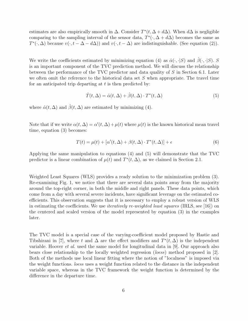
estimates are also empirically smooth in ∆. Consider T ∗(t, ∆ + d∆). When d∆ is negligiblecomparing to the sampling interval of the sensor data, T ∗(·, ∆ + d∆) becomes the same asT ∗(·, ∆) because v(·, t− ∆ − d∆)) and v(·, t− ∆) are indistinguishable. (See equation (2)).
We write the coefficients estimated by minimizing equation (4) as α(·, ·|S) and β(·, ·|S). Sis an important component of the TVC prediction method. We will discuss the relationshipbetween the performance of the TVC predictor and data quality of S in Section 6.1. Laterwe often omit the reference to the historical data set S when appropriate. The travel timefor an anticipated trip departing at t is then predicted by:
T (t, ∆) = α(t, ∆) + β(t, ∆) · T ∗(t, ∆) (5)
where α(t, ∆) and β(t, ∆) are estimated by minimizing (4).
Note that if we write α(t, ∆) = α′(t, ∆)+µ(t) where µ(t) is the known historical mean traveltime, equation (3) becomes:
T (t) = µ(t) + [α′(t, ∆) + β(t, ∆) · T ∗(t, ∆)] + ε (6)
Applying the same manipulation to equations (4) and (5) will demonstrate that the TVCpredictor is a linear combination of µ(t) and T ∗(t, ∆), as we claimed in Section 2.1.
Weighted Least Squares (WLS) provides a ready solution to the minimization problem (3).Re-examining Fig. 1, we notice that there are several data points away from the majorityaround the top-right corner, in both the middle and right panels. These data points, whichcome from a day with several severe incidents, have significant leverage on the estimated co-efficients. This observation suggests that it is necessary to employ a robust version of WLSin estimating the coefficients. We use iteratively re-weighted least squares (IRLS, see [16]) onthe centered and scaled version of the model represented by equation (3) in the exampleslater.
The TVC model is a special case of the varying-coefficient model proposed by Hastie andTibshirani in [7], where t and ∆ are the effect modifiers and T ∗(t, ∆) is the independentvariable. Hoover et al. used the same model for longitudinal data in [9]. Our approach alsobears close relationship to the locally weighted regression (loess) method proposed in [2].Both of the methods use local linear fitting where the notion of ”localness” is imposed viathe weight functions. loess uses a weight function related to the distance in the independentvariable space, whereas in the TVC framework the weight function is determined by thedifference in the departure time.
6

2.3 Implementation issues
There are several issues that we have to confront in order to put our method to use in realisticscenarios. For example, how do we get speeds to compute T ∗? What about the travel timesT (tn) for historical trips if they are not directly measured? How to deal with missing data?In this sub-section, we discuss potential solutions to these issues.
2.3.1 Data requirements
There are two distinct stages when applying the TVC travel time prediction method. In thefitting stage, model coefficients α(·, ·) and β(·, ·) are estimated by minimizing (4) using thehistorical data. The travel time predictor is then constructed from equation (5) with thecoefficients estimated in the fitting stage and T ∗ based on incoming data, in the predictionstage. We require T ∗ in both of the stages, while the historical trip travel time T (·) is onlyrequired in the fitting stage.
Computing T ∗ We define T ∗ in terms of measured speeds at each sensor location inequation (2). However, many widely-used sensors (for example, the single loop detector)provide only flows and occupancies, but not speeds. The conventional method to estimatespeeds from low-resolution flow and occupancy data is:
speed =flow
occupancy × g(7)
where g is assumed to be a constant related to the average vehicle length and must becalibrated for each test site. The usual approach to calibrate g is to backsolve g from (7)using an assumed free flow speed and measured flow and occupancy during a time period oflight traffic. Hall and Persaud [6] demonstrated that this approach produces a biased speedestimate where the bias is related to sensor location, time, and others factors.
We adopted an adaptive approach 2 in calibrating the g factor. The calibration is carriedout dynamically for each sensor. This approach partially compensates the dependency of gon time and location. The calibration procedure is described below. Let T be the samplinginterval. o(xl, ti) and q(xl, ti) are the flow and occupancy measured by the sensor at xl andtime ti = iT .
2 The approach is proposed by Zhanfeng Jia, Department of Electrical Engineering and ComputerScience, University of California at Berkeley
7

(1) For each sensor, the instantaneous g-factor is defined as:
ginst(xl, ti) =o(xl, ti)
q(xl, ti)vfree
where vfree represents the free flow speed and is usually taken to be 60 mph. ginst(xl, ti)is the result of applying the conventional calibration approach to sensor xl at ti = iT .
(2) ginst(xl, ·) is subject to significant bias when the traffic is congested. Assuming that gevolves slowly, we can use ginst(xl, ·) from the past when the traffic is congested. Weconsider that congestion is in procession when o(xl, ti) is above a threshold Othresh.We also smooth ginst(xl, ·) with an exponential filter to eliminate short-term variations.Formally,
gfilt(xl, ti) =
gfilt(xl, ti−1) if o(xl, ti) > Othresh
(1 − p)gfilt(xl, ti−1) + pginst(xl, ti) if o(xl, ti) ≤ Othresh
(8)
(3) The step above amounts to filter ginst(xl, ·) with a causal IIR filter which introducesdelay in the filtered factor gfilt(xl, ·). That is, gfilt(xl, ti + ρT ) is best suited to computethe speed at time ti and location xl using (7), where ρT is the time delay caused bythe exponential filter and is determined by p. We use the filtered factors from previousdays to estimate the differences between gfilt(xl, ti + ρT ) and gfilt(xl, ti). That is,
g(xl, ti) = gfilt(xl, ti + ρT )
= gfilt(xl, ti) + [gfilt(xl, ti + ρT ) − gfilt(xl, ti)]
= gfilt(xl, ti) +i+ρ∑j=i
[gfilt(xl, tj+1) − gfilt(xl, tj)]
u gfilt(xl, ti) +i+ρ∑j=i
g′(xl, tj)
(9)
where g′(xl, tj) = g(old)filt (xl, tj+1)−g
(old)filt (xl, tj) is computed using the filtered factors from
previous days.
We then plug g(xl, t) into equation (7) to compute the speed at location xl and time t fromflow and occupancy measurements. Compared with the conventional approach of assuming aconstant g-factor, the adaptive g-factor calibration significantly improves the accuracy of theestimated speeds. We use the resulting speeds to compute the current travel time predictorT ∗(t, ∆) from equation (2). This approach is applied to the District 12 data in Section 6.
Imputing T (t) The travel time T (t) can only be directly observed from probe vehicledata ([18]), AVI data ([19]) or other forms of vehicle tracking or re-identification data. Manylegacy data sets do not include such types of data. Here we describe a scheme to impute T (t)
8

from speeds at each sensor. The idea is to construct a hypothetical vehicle trajectory usingthe observed speeds. Again v(xl, t) is the speed at time t and location xl. Then,
τ0 = t; (10)
τ1 = τ0 +x1 − x0
v(x0, τ0);
. . .
τl+1 = τl +xl+1 − xl
v(xl, τl);
. . .
τL = τL−1 +xL − xL−1
v(xL−1, τL−1);
T (t) = τL − τ0
Equation (10) is well suited for computing T (tn) for historical trips, where all speeds neededin the equation are available. We can also apply this scheme to accurately estimated speeds,such as those from the adaptive g-factor approach introduced earlier.
The quality of the imputed T (t) is certainly related to the quality of the speeds used inequation (10). However, even if the speeds at the sensor locations are accurate, the imputedT (t) might not be so when the link lengths are very long. The reason is that equation (10)implicitly assumes that the average speed within a link is close to the speed at the upstreamsensor. The assumption is fine when the prevailing speed does not change rapidly withinthe scope of a link. When a link covers a long distance, it is more likely that the implicitassumption does not hold, especially during congestion time periods when the traffic is morevolatile. Fig. 2 illustrates the possible error of the imputed T (t). Because of the exception-ally long link AB, we are unable to observe the speed changes in the path of the anticipatedtrip (the thick solid line in Fig. 2). As a result, the projected track (the dash line) and theimputed T (t) are far from acceptable. Fig. 2 also indicates that the anticipated departuretime is related to the accuracy in the imputed T (t), since traffic conditions are more volatilefor trips initiated during rush hours.
The above strategies allow us to impose minimal restrictions on the source of data. While therecent advances in traffic surveillance technologies may reduce the need for these procedures,implementing new traffic surveillance systems often requires commitment of huge amountsof financial and human resources. It is therefore wasteful and sometimes impossible to ignoredata from previously-installed infrastructures such as single loop detectors. Our approachcan be applied without modification to hybrids of different types of sensor data. In Section 4we present examples where T ∗ is computed using double-loop speeds and the historical traveltimes are from probe vehicle data, while the results in Section 6 are solely based on single
9

error
TimeStart
End
A
B
Fig. 2. Conceptual illustration of the possible error from the imputed T (t). The X-axis representsthe temporal axis, and the Y-axis is the spatial axis, with the trip going upwards. The shadowedrectangle between point A and B marks one exceptionally long link with no sensor in between.The irregular shape in the middle represents a temporal-spatial region of congestion where theprevailing speed is slower. The thick solid line represents the actual track of a vehicle. Notice thatthe vehicle slows down after entering the shadowed congestion region. The dash line is the vehicletrack projected by equation (10) using the speeds from the sensors. Since there is no sensors betweenA and B, equation (10) projects the arrival at the sensor B using the non-congested speed from thesensor A. This results in error in the imputed T (t) as illustrated in the figure.
loop measurements at 30 second resolution.
2.3.2 Data quality issues
Missing or corrupted sensor data are unavoidable in practice. We use linear interpolationalong space to impute speeds for a missing detector from values of neighboring detectors.Nonetheless, the quality of T ∗ (and/or the historical travel times, if they are computed usingequation (10)) becomes questionable when the unusable data are prevalent. We demonstratethe negative impact of missing data on the prediction accuracy of the TVC method in Sec-tion 6.1.
Interestingly, the TVC method may be applied to the situation where sensors do not coverthe entire trip, with only minor modifications. This is applicable when we use the historicaltravel times from a data source independent of the sensor data that are the basis of T ∗, orwhen the learning set 3 contains T ∗ for the entire trip but some data are missing at the time
3 The historical data set used to estimate model coefficients
10

a prediction is to be made. Suppose that the sensors cover effectively only a non-trivial sub-section AB of the complete trip. Let T ∗
AB(·, ·) be the current travel time predictor for AB.Substitute T ∗ with T ∗
AB in equation (4) to get estimated coefficients αAB(·, ·) and βAB(·, ·).Plug T ∗
AB(t, ∆) together with these estimated coefficients into (5) to get the predicted traveltime for the entire trip. When AB includes all strategically important locations (bottlenecks,merging points et cetera) and covers a significant portion of the entire trip, it is likely thatthis modified TVC method will be satisfactory.
3 Performance measure and baseline predictors
To understand the performance of the TVC travel time predictor, it is important to com-pare it to other predictors. In particular, we consider two baseline travel time predictors –one is the current travel time predictor T ∗ which relies solely on current traffic information,the other is the mean historical travel time. If the TVC method does not show significantimprovements over the baseline predictors, there is no merit in adopting the method.
We use the Mean Average Percentage Prediction Error (MAPPE) to quantify the perfor-mance of a predictor. We introduce the definition of MAPPE in Section 3.1. In Section 3.2, wepresent MAPPE estimators for the TVC predictor. Finally, we discuss the baseline predictorsin Section 3.3.
3.1 Mean Absolute Percentage Prediction Error (MAPPE)
We define the following terminology for a candidate travel time predictor T PRED(t).
Definition 3.1. Let γ(t, T PRED(t)) be the percentage prediction error (PPE) of T PRED(t).γ is defined as:
γ(t, T PRED(t)) =T (t)− T PRED(t)
T (t)
γ is the signed relative prediction error for an individual trip.
Definition 3.2. The Mean Average Percentage Prediction Error (MAPPE) for the predictorT PRED(t) is E |γ(t)|, where the expectation is over the sample space of all trips.
MAPPE measures the magnitude of the relative error over the entire temporal spectrum. Itprovides a unit-free measure of the performance characteristics of a prediction method. Itcan be used to compare predictions across different test sites.
11
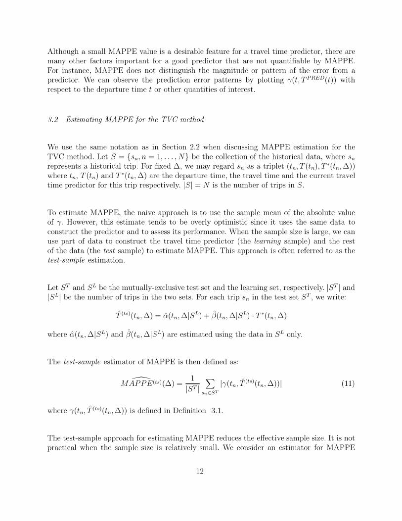
Although a small MAPPE value is a desirable feature for a travel time predictor, there aremany other factors important for a good predictor that are not quantifiable by MAPPE.For instance, MAPPE does not distinguish the magnitude or pattern of the error from apredictor. We can observe the prediction error patterns by plotting γ(t, T PRED(t)) withrespect to the departure time t or other quantities of interest.
3.2 Estimating MAPPE for the TVC method
We use the same notation as in Section 2.2 when discussing MAPPE estimation for theTVC method. Let S = {sn, n = 1, . . . , N} be the collection of the historical data, where sn
represents a historical trip. For fixed ∆, we may regard sn as a triplet (tn, T (tn), T∗(tn, ∆))
where tn, T (tn) and T ∗(tn, ∆) are the departure time, the travel time and the current traveltime predictor for this trip respectively. |S| = N is the number of trips in S.
To estimate MAPPE, the naive approach is to use the sample mean of the absolute valueof γ. However, this estimate tends to be overly optimistic since it uses the same data toconstruct the predictor and to assess its performance. When the sample size is large, we canuse part of data to construct the travel time predictor (the learning sample) and the restof the data (the test sample) to estimate MAPPE. This approach is often referred to as thetest-sample estimation.
Let ST and SL be the mutually-exclusive test set and the learning set, respectively. |ST | and|SL| be the number of trips in the two sets. For each trip sn in the test set ST , we write:
T (ts)(tn, ∆) = α(tn, ∆|SL) + β(tn, ∆|SL) · T ∗(tn, ∆)
where α(tn, ∆|SL) and β(tn, ∆|SL) are estimated using the data in SL only.
The test-sample estimator of MAPPE is then defined as:
MAPPE(ts)(∆) =1
|ST |∑
sn∈ST
|γ(tn, T(ts)(tn, ∆))| (11)
where γ(tn, T(ts)(tn, ∆)) is defined in Definition 3.1.
The test-sample approach for estimating MAPPE reduces the effective sample size. It is notpractical when the sample size is relatively small. We consider an estimator for MAPPE
12

based on a modified version of cross validation, which was used in [11].
In a nutshell, we treat one day as the test set and the remaining days as the learning set.We then construct a predictor using the learning set and compute γ for each trip in the testset. MAPPE is estimated by averaging the absolute values of γ’s computed this way. Theapproach partially accounts for the dependence between data points collected on the sameday.
The cross-validation estimator of MAPPE for the TVC method is constructed as follows:
(1) For each trip sn in S, let dn be an ordinal number identifying the day on which sn wasmade. Define
S(−n) = {sm ∈ S, dm 6= dn}That is, S(−n) is the subset of S that contains all the trips made on a different day asthe nth trip sn.
(2) WriteT (cv)(tn, ∆) = α(−n)(tn, ∆|S(−n)) + β(−n)(tn, ∆|S(−n)) · T ∗(tn, ∆)
where the coefficients α(−n)(tn, ∆|S(−n)) and β(−n)(tn, ∆|S(−n)) are estimated with onlythe data in S(−n).
(3) Let γ(cv)n represent the percentage prediction error for the cross-validation travel time
predictor defined in the last step.
γ(cv)n (∆) = γ(tn, T
(cv)(tn, ∆)) =T (tn) − T (cv)(tn, ∆)
T (tn)(12)
(4) Repeat the above steps for each trip to get γ(cv)1 , γ
(cv)2 , . . . , γ
(cv)N . The cross-validation
MAPPE estimate at ∆ is:
MAPPE(cv)
(∆) =1
N
N∑n=1
|γ(cv)n (∆)| (13)
3.3 The baseline predictors
The TVC travel time predictor T (t, ∆) uses both historical travel time information andcurrent freeway sensor data. The historical information comes into play in the form of theestimated coefficients α(t, ∆) and β(t, ∆). Current freeway sensor data are summarized byT ∗(t, ∆). We may consider predictors which rely solely on historical information (or currenttraffic measurements) as baseline predictors. Intuitively, T (t, ∆) should outperform the base-line predictors since it is based on an enlarged information set. The degree of performance
13

improvement over the baseline predictors are indicated by the difference in such performance-measuring statistics as MAPPE discussed in Section 3.1.
As mentioned before, T ∗(t, ∆) is a travel time predictor using current traffic data only. Toestimate MAPPE for this predictor, we use the naive plug-in estimate for MAPPE, sincecross validation is not applicable in this case.
MAPPE∗(∆) =1
|S|∑
sn∈S
∣∣∣∣∣T (tn) − T ∗(tn, ∆)
T (tn)
∣∣∣∣∣ (14)
For an example of predicting travel times with historical information alone, consider thefollowing predictor for T (t):
T H(t|S) =
∑sn∈S T (tn) · I(|tn − t| ≤ 5 min)∑
sn∈S I(|tn − t| ≤ 5 min)(15)
where I(·) is an indicator function that evaluates to one when |tn − t| ≤ 5 min. T H(t) isthe mean historical travel time for all trips departing within five minutes of t. (For instance,we predict the travel time at 9AM by the mean travel time of all historical trips departingbetween 8:55AM and 9:05AM.) The plug-in MAPPE estimate for the predictor in (15) is:
MAPPEH =1
|S|∑
sn∈S
∣∣∣∣∣T (tn) − T H(tn|S)
T (tn)
∣∣∣∣∣ (16)
Note that MAPPEH is not related to ∆. MAPPEH tends to overstate the accuracy ofT H(·|S) since they are based on the same historical data set S. We can adopt the test sample
approach for T H(·|S) when appropriate. The test-sample MAPPE estimator is defined as:
MAPPE(ts)
H =1
|ST |∑
sn∈ST
∣∣∣∣∣T (tn) − T H(tn|SL)
T (tn)
∣∣∣∣∣ (17)
where ST and SL are the test and learning data set, respectively. T H(·|SL) is the histori-cal mean computed using the learning set only, and is constructed by replacing S with thelearning data set SL in equation (15).
Table 1 summarizes the notation and the equation references of the MAPPE estimators. InSection 4 and Section 6, we will sometimes compare re-substitution MAPPE estimators forthe baseline predictors with the test-sample (or cross-validation) MAPPE estimator for theTVC method. One should bear in mind that the re-substitution MAPPE estimator tends tooverstate the prediction accuracy.
14

Prediction Method Re-substitution Test sample Cross validation
TVC - MAPPE(ts)
(∆), (11) MAPPE(cv)
(∆), (13)
Historical mean MAPPEH , (16) MAPPE(ts)
H , (17) -
T ∗ MAPPE∗(∆), (14) - -
Table 1Notations and equation numbers of the MAPPE estimators.
4 Results – Part 1
In this section we illustrate, by example, the application of our methodology to actual free-way data. The data set includes high-quality data from double loop detectors and probevehicles, yet it is limited in both spatial and temporal scales. It gives us a chance to test theeffectiveness of our method before moving on to larger, more complex data sets. Kwon etal. [11] used the same data set to compare another linear model approach with decision-treebased methods.
The data comes from a six mile section of highway I-880 in Hayward, California ([18], [20]).This section of freeway was instrumented with 35 double-loop detector stations spaced ap-proximately 1/3 miles apart. Here we used the north-bound data collected between 5am and10am in the morning. There were 18 detector stations monitoring the north-bound traffic.The raw data were collected every one second, but we aggregated the data to thirty secondresolution before further analysis. We computed the current travel time predictor T ∗(t, ∆)using speeds measured by double-loop detectors from equation (2).
In addition to the loop detector data, there were up to four probe vehicles driving up anddown the freeway section during commute hours. The probe vehicles, which maintained aheadway of approximately 7 minute headway, were equipped with computers that accuratelyrecorded vehicular movements, and hence travel times. The probe vehicle travel times areimportant since they are the only measured (versus estimated) travel times available in thisexperiment. In the examples in this section, we used the observed probe vehicle travel timeas T (t).
The data set has 364 trips on 20 weekday mornings between 2/22/1993 and 3/19/1993.Fig. 3 plots the probe vehicle travel T (tn) time against the departure time tn. The figureshows that congestion generally occurred between 7am and 9am, and may cause up to 50%increase of travel time on a typical day. The thicker solid line highlights the traffic profileon 3/10/1993, when multiple severe incidents hit the test region. We regard 3/10/1993 as
15

6:00 6:30 7:00 7:30 8:00 8:30 9:00 9:30 10:00
6
8
10
12
14
16
18
20
22
Departure time
Tra
vel t
ime
(min
)
I−880 data: 20 days, 364 runs
Fig. 3. The I-880 data. The figure plots probe vehicle travel time T (t) versus departure time t. Eachline corresponds to a day. There are 20 lines in the figure. The thicker solid is for March 10, 1993.Multiple severe incidents happened on that day; the thicker dash line is for March 11, 1993 – oneof the days chosen to represent the recurring congestion at the test site.
an example of a “bad” day, which is distinguished by worse than usual congestion due toaccidents or other uncommon events. We call days with normal recurring congestion the“normal” days. 3/11/1993 is such a day and is marked by the thick dash line in Fig. 3.
We organize this section as follows: In Section 4.1, we compare the estimated mean absolutepercentage prediction error (MAPPE) of the TVC method and the two baseline predictors.It is followed by contrasting the predicted travel time profiles on a “normal” day (3/11/1993)versus those on a “bad” day (3/10/1993) in Section 4.2. In Section 4.3 we investigate theempirical temporal patterns of the prediction error from the TVC method.
4.1 Comparing MAPPE
The mean absolute percentage prediction error (MAPPE) measures the accuracy of a traveltime predictor averaging over all data points regardless of their departure times. By com-paring MAPPE based on the same data set, we gain understanding about the differences inthe overall prediction accuracy of candidate prediction methods.
Here we compare the estimated MAPPE values for the TVC predictor T (t, ∆) with those
16

of the historical mean baseline T H(t) and the T ∗(t, ∆) baseline, at different values of ∆. InSection 3, we presented details on estimating MAPPE for the three predictors. Due to therestricted sample size, we use cross validation to estimate MAPPE for the TVC method. Weuse the more-optimistic re-substitution MAPPE estimators for the two baseline predictors.
That is, we examine MAPPE(cv)
(∆) in relation to MAPPE∗(∆) and MAPPEH, using thenotation summarized in Table 1.
Fig. 4 plots the estimated MAPPE values against ∆, where ∆ ranges from zero up to 60minutes. Fig. 4 shows that the overall prediction quality for both the TVC method andthe T ∗ baseline deteriorates when ∆ increases. The observation reflects that the associationbetween the present traffic scenario (as represented by T ∗(t, ∆)) and the anticipated onegrows weaker as ∆ increases. At any value of ∆, the TVC method dominates the current
travel time predictor T ∗ in terms of estimated MAPPE. The gap between MAPPE∗(∆) and
MAPPE(cv)
(∆) increases from about 1% at ∆ = 0 to more than 10% when ∆ is over 40minutes. The figure clearly indicates that the TVC method is favorable to the T ∗ baselinepredictor.
The estimated MAPPE for the TVC method displays a slightly convex shape. MAPPE(cv)
(∆)increases steadily from roughly 6% at ∆ = 0 to about 11% at ∆ = 30 minutes and then sta-bilizes at a value slight higher than the re-substitution estimator for the historical mean. Thefigure suggests that the TVC method is preferable to the historical mean when ∆ is small(≤ 20 minutes), but the favorable edge diminishes gradually as we predict further ahead andvanishes after ∆ = 30 minutes. It looks as if ∆ = 30 minutes is the point beyond whichthe current traffic information captured by the data up to t − ∆ becomes so remote thatit does not help in predicting the anticipated travel time T (t). Note that at 11% the TVCmethod is well within the accuracy requirements of many important transportation appli-cations including home-based route planning and in-car vehicle information systems (cf. [22]).
The results in this sub-section support the applicability of the TVC travel time predictionmethod. The performance of the TVC predictor is significantly better than than both ofthe baseline predictors for short-term prediction, and is still on par with the historical meanbaseline when we predict more than 30 minutes ahead on a 6 mile freeway section. As a by-product of our analysis, we found that the current travel time profile T ∗(·, ∆) is satisfactoryonly for moderate-to The observations in this section are consistent with the notion that thecurrent traffic information is more valuable for short-term forecasting.
17

0 10 20 30 40 50 605
10
15
20
25
Delta (min)
MA
PP
E (
%)
MAPPE: estimated by Cross Validation
Time−varying coefficient modelHistorical mean T*
Fig. 4. Mean Average Percentage Prediction Error (MAPPE) using the I-880 data set. The X-axis isthe temporal look-ahead parameter ∆, the Y-axis is the estimated MAPPE. The solid line represents
MAPPE(cv)
(∆) from equation (13); the thin dash line for MAPPE∗(∆) (equation (14)) and thethick horizontal line for MAPPEH (equation (16)). Note that the line for MAPPEH is flat sincethe historical mean predictor does not use current traffic data and is hence not related to ∆.
4.2 Patterns in predicted travel times
It is desirable that a travel time predictor should capture the anticipated traffic pattern.This is especially important for automatic incident detection because the ability to detectchange in traffic patterns and the accuracy in doing so determine the performance of suchsystems. Using a historical profile in such systems is not feasible.
To illustrate the similarities and differences between the traffic patterns demonstrated bythe predicted travel times and the actual ones, we plot the actual travel time together withthe predicted travel times from the TVC method and the historical mean baseline predictoras time series. We did not include the current travel time predictor T ∗(t, ∆) in this part ofthe analysis since the evidences in Section 4.1 have demonstrated that it is inferior to boththe TVC predictor and the historical mean predictor. Fig. 5 shows these plots for differentvalues of ∆ on two selected days. The three left-side panels in the figure are for the “normal”day 3/11/1993. The right panels represent the “bad” day 3/10/1993 – a Wednesday marredby several traffic-disrupting incidents at the test site.
18

6:30 7:00 7:30 8:00 8:30 9:00 9:30
6
8
10
12
14
16
18
20
22
departure time
trav
el ti
me
(min
)03/11/1993, Delta = 0 min
"Actual" Historical mean Time−varying coefficient model
6:30 7:00 7:30 8:00 8:30 9:00 9:30
6
8
10
12
14
16
18
20
22
departure time
trav
el ti
me
(min
)
03/10/1993, Delta = 0 min
"Actual" Historical mean Time−varying coefficient model
6:30 7:00 7:30 8:00 8:30 9:00 9:30
6
8
10
12
14
16
18
20
22
departure time
trav
el ti
me
(min
)
03/11/1993, Delta = 20 min
"Actual" Historical mean Time−varying coefficient model
6:30 7:00 7:30 8:00 8:30 9:00 9:30
6
8
10
12
14
16
18
20
22
departure time
trav
el ti
me
(min
)
03/10/1993, Delta = 20 min
"Actual" Historical mean Time−varying coefficient model
6:30 7:00 7:30 8:00 8:30 9:00 9:30
6
8
10
12
14
16
18
20
22
departure time
trav
el ti
me
(min
)
03/11/1993, Delta = 40 min
"Actual" Historical mean Time−varying coefficient model
6:30 7:00 7:30 8:00 8:30 9:00 9:30
6
8
10
12
14
16
18
20
22
departure time
trav
el ti
me
(min
)
03/10/1993, Delta = 40 min
"Actual" Historical mean Time−varying coefficient model
Fig. 5. Comparison of travel time predictors. The X-axis is the departure time t. The Y-axis isT (t) and corresponding predicted travel times from the time-varying coefficient method and thehistorical mean. The top, middle and bottom left panels plot the predictors for ∆ = 0, 20, 40minutesrespectively on March 11, 1993 – a day with representative recurring congestion. The three rightpanels are for March 10, 1993 – a Wednesday with several significant traffic incidents in the testarea. In all panels, the thick line is the actual travel time T (t) from probe vehicle data; the linewith the x mark is the predicted travel time T (t, ∆) and the thinnest line represents the historicalmean travel times for all available data. Note that this line is the same for all panels.
19

The historical mean travel time is represented by the thinnest line in the panels. It is thesame in every panel since it is computed using all available data. The thickest solid linesshow the actual travel times T (t) from probe vehicle data, while the line marked with x isT (t, ∆) from the TVC method. The top, middle and bottom panels are for ∆ = 0, 20 and 40minutes respectively. Note that for panels in the same column, only the x-marked lines aredifferent.
Let us first study the three right-side panels of Fig. 5. These panels are for the “bad” day3/10/1993 with multiple severe incidents. Expectedly, the historical profile is far from theactual one in this case. For the TVC method, we observe that it accurately grasps the actualtraffic pattern when we use all the data up until the anticipated departure time (∆ = 0).The middle-right panel suggests that at ∆ = 20 minutes the TVC still catches some of theaccident-induced traffic delay, only after an appreciable delay. When ∆ = 40 minutes, wecan hardly find any trace of the actual traffic pattern from the information conveyed by theTVC predicted travel time. From the top to the bottom panels, the peak region in the TVCpredicted profile occurs later in time and also decreases in magnitude.
The three left-side panels (for the “normal” day 3/11/1993) tell a different story. The histor-ical mean profile is fairly close to the actual one here. Upon closer examination, we observethat the recurrent congestion on this day started somewhat earlier than average, by compar-ing the actual travel time profile and the historical mean. At ∆ = 0, the TVC predictor picksup the early congestion between 7:30am and 7:45am well. However, both the TVC methodat ∆ = 20 or 40 minutes (two bottom panels on the left), and the historical mean predictorunderstate the congestion in the same time period.
The example here shows that although the historical mean predictor is reasonable on a“normal” day, it is totally inadequate for a day with significant incidents. On the otherhand, the TVC method is capable of capturing the anticipated traffic profile even underunfavorable traffic conditions for small values of ∆.
4.3 Temporal behavior of the prediction error
Based on the findings of Section 4.1 and Section 4.2, we conclude that the TVC methodis preferable to both the current travel time predictor T ∗ and the historical mean. In thissection we further our investigation by examining the temporal behavior of the travel timeprediction error from the TVC method. In particular, we seek answers to the following ques-tions: Is the TVC method prone to larger errors when the anticipated trip coincides withthe rush hours, or on a day plagued by accidents or other external events? How does the
20

magnitude of the prediction error depend upon the time of day? In other words, we try tounderstand the relationship between the prediction accuracy and factors such as the depar-ture time or the occurrence of incidents.
We quantify the prediction accuracy by the percentage (or relative) prediction error γ de-fined in 3.1. As in Section 3.1, we use the leave-one-day-out cross validation in computing γfrom the historical set. That is, we consider γ(cv)
n (∆) as in Equation (12) on page 13.
Fig. 6 depicts the relationship between the departure time t and γ(cv)n (∆) for ∆ = 0. The
figure is plotted as follows: As in Section 3.1, let S = sn, n = 1, . . . , N be the set of historicaltrips. Bin the trips in S according to the departure time of sn. We then plot the summarystatistics of γ(cv)
n for the trips in each bin against the center of the bin. Specifically, the thickline is the median, the two thinner lines are the 25th and 75th percentiles of γ respectively.The vertical lines represent the ranges of γ. Fig. 6 reveals that the relative prediction erroris mostly within the 10% bracket during the time period studied. The inter-quartile rangeof γ (as shown by the two thinner lines) increases slightly between 7:30am and 8:45am. Ex-treme values are also larger during this time interval than before and after. The observationsupports the assertion that the TVC travel time predictor tends to be less reliable if the
6:30 7:00 7:30 8:00 8:30 9:00 9:30
−50
−30
−10
0
10
30
50
2 3
9
12
1226 15 16
17 20 11
17
15
25
14
11
19
13
20
13
1717
20
19
1
Departure time
Per
cent
age
pred
ictio
n er
ror
(%)
Delta = 0 min
0 2 4 6 8 10 12 14 16 18 20
−0.4
−0.2
0
0.2
0.4
0.6
Day
Rel
ativ
e pr
edic
tion
erro
r (%
)
Relative error, Delta = 0 min
Fig. 6. Relationship between the absolute per-centage prediction error γ(t, ∆) and the depar-ture time t for ∆ = 0. The X-axis is the depar-ture time. The thick line represents the median.The two thinner lines are the 25th and 75 per-centiles respectively. The vertical lines depict therange of γ(t, ∆). The numbers at the bottom ofthe vertical lines are the sample size used.
Fig. 7. Day-to-day variation of percentage pre-diction error (PPE) from the TVC method when∆ = 0. The vertical lines represent the range ofPPE for each day. The horizontal bar on eachvertical line marks the daily median PPE, whilex marks the 25th and 75th percentiles for PPEon each day. Dots on the vertical lines mark PPEoutside of the daily interquartile range. The twodotted reference lines are the ±10% lines.
21

anticipated trip departs during the rush hours.
We use a similar graphical method to depict the day effect on γ(t, ∆) to gauge the degreeof the effect of external events (such as accidents) on the prediction accuracy. We divide thehistorical data set S into 20 mutually-exclusive subsets Si. Each of the subset Si is consistedof all trips on day i. For the I-880 data set, we have twenty such subsets. We plot the sum-mary statistics of γn for trip in each subset Si versus the day index i. See Fig. 7 for theresulted plot when ∆ = 0.
Fig. 7 indicates that the TVC method is quite accurate on most days – the interquartile rangeof γ is well within [−10%, +10%] on all 20 days. However, the figure shows that the TVCmethod does not behave so well on the 13th and the 18th day (3/10/1993 and 3/17/1993respectively). Indeed these two days are distinguished from the other days by severe inci-dents. This indicates that the occurrence of accidents has a significant negative impact onthe prediction accuracy of the TVC model.
Similar plots as Fig. 6 and Fig. 7 for larger values of ∆ (not shown) display similar patternsas what we observe here. We find that the TVC method is less accurate during congestedhours and when significant incidents are present in the anticipated trip. How to use thefindings here to enhance our model is a direction of future research.
5 Extensions
In this section, we introduce several pragmatic extensions to the TVC model and method. InSection 5.1 we first discuss how to assemble the predicted travel time for a trip consisted ofmultiple sub-segments from the travel times of individual sub-segments. We then consider aproxy for the current travel time predictor when accurate speed estimates are not available,in Section 5.2.
5.1 Segmenting a trip
The TVC model (defined by (3)) is built on top of highly reduced data. In Section 2.1 wehave shown that the current travel time predictor T ∗(·, ·) summarizes the high-dimensionalraw sensor readings. In many cases, the response variable T (t) itself is the sum of travel timesfor sub-segments of the trip. The TVC method ignores some of the available information viathe implicit data reduction.
22

The TVC travel time predictor uses the linear association between T (t) and T ∗(t, ∆) and itsprediction accuracy is directly linked to the strength of the association. For longer trips, theassociation is weaker because of more complex traffic scenarios. It is therefore interesting toconsider if we can recoup some of the unused information and thus improve the predictionaccuracy by applying the TVC method to sub-segments of the trip.
����A -
����B -
����C
Fig. 8. A stretch of freeway divided into two sub-segments.
Fig. 8 shows a trip AC consisted of two sub-segments AB and BC . We use the notationTABC to represent the travel time predictor for AC by assembling those for the sub-segmentsAB and BC , where the subscript signifies the division of the trip into two sub-segments. Weconstruct TABC as:
TABC(t, ∆) = TAB(t, ∆) + TBC(t + TAB(t, ∆), ∆ + TAB(t, ∆)) (18)
Note that the part of the predicted travel time in (18) attributed to the second sub-segmentdepends on that to the first sub-segment.
The formulation of TABC(t, ∆) is similar to that of (10) in Section 2.3 – that is, by projectinga hypothetical arrival time at the intermediate node B according to the predicted travel timeof the previous sub-segment. In the same fashion, we can construct a travel time predictorwhen the trip is divided into an arbitrary number of sub-segments. Equation (18) may alsobe applied to an arbitrary route in a complex roadway network, such as the highlighted routeA (Irvine) to C (east of Garden Grove) via B in Fig. 9. Each leg in the route may be dividedinto further sub-segments.
The discussion here naturally leads to the question of if and how to divide a trip into sub-segments. In the extreme case, we may apply the method link by link where each link isdelimited by a pair of adjacent sensors. The question is analogous to the model selectionproblem, and it may be worthwhile to look for inspirations in the rich statistical model selec-tion literature ([1], [12]). Essentially the number of parameters in the TVC model increaseswith the number of sub-segments. By dividing the trip with many sub-segments, we mightbe able to reduce the systematic bias of the model, but run higher risk of over-fitting thehistorical data. On the other hand, the TVC model with no segmenting may be too scant todescribe all the variability for a long trip. The question is to look for the optimal segmenta-tion of a trip. We do not endeavor to address this issue here. In Section 6.2, we present anexample that compares the travel time predicted from (18) to that from applying the TVC
23

method directly to the entire trip. There we will also discuss some hunches on segmenting atrip.
5.2 The quasi current travel time predictor
When we introduced the definition of the current travel time predictor T ∗(·, ·) in Section 2.1,we assumed that speeds are directly measurable. In Section 2.3.1, we described a remedy forsensors that only measure flows and occupancies (such as single-loop detectors). However,this remedy still requires careful calibration/estimation of the g factor for each individualsensor. Here we introduce a quasi current travel time predictor T (·, ·) that relies on flowsand occupancies only.
Equation (7) suggests that the ratio of flow to occupancy is approximately proportional tothe speed. We define the quasi speed v as:
v(xl, t) =q(xl, t)
o(xl, t)(19)
where q(xl, t) and o(xl, t) are the flow and occupancy measured by the sensor located at xl
at time t. The quasi current travel time predictor T (t, ∆) is defined by replacing v(·, ·) inequation (2) with v. Note that v is the same as the estimated speed from equation (7) wheng = 1. Therefore, the quasi current travel time predictor T (t, ∆) is proportional to the cur-rent travel time predictor computed using estimated speeds by assuming a constant g-factorin (7). Hence T (t, ∆) may be regard as a proxy for T ∗(t, ∆) in the TVC methodology. Weconstruct a travel time predictor by replacing T ∗(·, ∆) with T (·, ∆) in equations (3), (4) and(5). We write the resulted travel time predictor using the T (·, ·) as T Q(·, ·). In Section 6.3,we will demonstrate by example that the behavior of T Q(·, ·) is quite close to that of T (·, ·)computed using T ∗.
Note that when flow and occupancy measurements are the only data available (such as atest site equipped with single loop detectors only), the adaptive calibration scheme of theg-factor should still be used to impute the travel time T (t) for the historical data. Adoptingthe quasi current travel time predictor in the TVC framework eliminates the necessity ofadaptively calibrating g for the incoming data, and hence speeds up the prediction process.
24

Fig. 9. Map of District 12.
25

6 Results – Part 2
In Section 4, we applied the TVC method to the I-880 data set. The results are quite en-couraging. However, the distance covered by the data set – less than six miles – is too shortto be interesting in practice. We need to put the method to further test scenarios that arecomparable to those arising in actual applications of travel time prediction.
The District 12 data set is a good testbed for this purpose. The test site is in Orange County(designated as District 12 by California Department of Transportation) in southern Califor-nia, about 15 miles south of Los Angeles City and County. In this section, we concentrateon studying the 20 mile long North-bound I-405 trip in the 5-10AM time period. The mapof the test site is shown in Fig. 9, where the studied trip (A to C) is highlighted by a darkershape of gray. We chose to study this particular section of the test site because its lengthis appropriate, and the data quality is relatively good compared to the other possible choices.
The data available are 30-second flow and occupancy measurements collected by single loopdetectors. As for many other loop detector data sets, data quality is a major problem evenfor the selected locale and time period. The original data involved in the examples in thissection are marred by considerable amount of missing data and various kinds of unspecifiedcorruption. We use the following procedure to exclude corrupted data, before computingspeeds from the raw flow and occupancy measurements:
(1) The flow and occupancy measurements are accompanied by a loop status flag whichindicates the functional aspects of the loop detector that outputs the measurements.We use data from loops where the status flag is either 1 or 2 (which signify more reliabledata) for the entire studied time period.
(2) There are detectors that output constant values for a sustained period of time. We ex-clude the data collected by any loop detector that output constant values consecutivelyfor more than sixty minutes during the five hour period that we study.
We use the data collected on weekdays between 2/1/1998 and 6/30/1998 for the resultspresented in this section. After filtering out unreliable data using the aforementioned pro-cedure, we are left with 56 days worth of data. The amount and locations of usable datavaries significantly from day to day. The daily average distance between adjacent detectorswith good data varies from 0.7 miles to 2.4 miles. On average 40% of the original data sur-vive the filtering process each day. Of the 56 available days, we randomly select 38 days asthe learning data and the remaining 18 days as the test data set. The data in the test andlearning sets are shown in Fig. 10. Overall there are 2006 trips in the learning set and 982trips in the test set.
26

5:00 5:30 6:00 6:30 7:00 7:30 8:00 8:30 9:00 9:30 10:00
20
40
60
80
100
120
140
Departure time
Tra
vel t
ime
(min
)District 12 training data: 38 days, 2006 runs
5:00 5:30 6:00 6:30 7:00 7:30 8:00 8:30 9:00 9:30 10:00
20
40
60
80
100
120
140
Departure time
Tra
vel t
ime
(min
)
District 12 test data: 18 days, 982 runs
(a) Learning data set SL. 38 days (b) Test data set ST . 18 days. The thickline represents 5/6/98. We presentexamples based on the day in Sec-tion 6.1.
Fig. 10. The District 12 data set. The panels plot the imputed T (t) (computed from (10) usingspeed estimated from equation (7), where g is estimated adaptively for each loop detector) versusthe departure time t. Each line corresponds to a day. The learning set is comprised of 38 daysrandomly selected from S. The test set has the remaining 18 days.
The quality of the District 12 data has important implications for our analysis:
• There are no actual observations of the travel time T (t) in this data set. We use equation(7) to estimate speeds from flow and occupancy measurements, where g is estimated everyfive minutes by the adaptive approach discussed in Section 2.3.1. The speeds thus estimatedin then used to compute the current travel time predictor T ∗(t, ∆), and also to impute theanticipated travel time T (t) from (10).
• Missing data is a severe problem for the District 12 data set. The longest links are nearly7 miles long on the worst days. This means that there are non-negligible errors in bothT ∗(t, ∆) and the imputed T (t). The situation may be conceptualized as follows:
T (t) = T (t)(true) + ε1(t)
T ∗(t, ∆) = T ∗(t, ∆)(true) + ε2(t)
where T (t)(true) and T ∗(t, ∆)(true) are the unknown “true” values of their counterpartsshould there be no missing data. The errors ε1(t) and ε2(t) are non-stationary and stronglycorrelated. The impact of these errors are difficult to quantify. Qualitatively, the associationbetween the contaminated T (t) and T ∗(t, ∆) tends to be weaker than that between theiruncontaminated counterparts 4 . Therefore, the TVC predictor would be more accurate
4 Suppose that there is a perfect linear relationship between T (t)(true) and T ∗(t, ∆)(true). Thecontamination of ε1(t) and ε2(t) renders the linear association between T (t) and T ∗(t, ∆) to be less
27

Mean Standard deviation
SL(G): Good learning data 0.8 0.1
SL(B): Bad learning data 1.4 0.4
SL = SL(G) ∪ SL(B): Learning data 1.1 0.4
ST : Test data 1.0 0.4
S = SL ∪ ST : All data 1.1 0.4
Table 2Summary statistics of the average link length for the District 12 data set.
should the uncontaminated values of T (t) and T ∗(t, ∆) be available.• In the examples in this section, we compare two different versions of the TVC method by
comparing their MAPPE values estimated using the test sample approach (cf. Section 3).It is unclear how the estimated MAPPE values are affected by the data quality problemsin the test sample. MAPPE is estimated by taking the average of the percentage predictionerror (PPE) for every trip in the test sample. Since the errors in T (t) and T ∗(t, ∆) tend tobe significant only for those trips immediately before or after the occurrence of congestion,the PPEs for many of the trips in the test sample might not be far from the truth. Hence, itis possible that the estimated MAPPE values are not subject to severe errors. Furthermore,it is unlikely that a randomly-selected test sample would bias in favor of one of the methodsbeing compared.
• However, because the potential error in the T (t) is related to the departure time, it may beproblematic to examine the relationship between the percentage prediction error and thedeparture time, or its day-to-day variations (i.e. the analysis conducted in Section 4.3).We omit those analysis in this section.
In Section 6.1, we investigate the effects of learning data quality on prediction accuracyby contrasting the TVC predicted travel times using two learning data sets with differentamounts of missing data. We then examine the extensions to the TVC method in the twofollowing sections. We illustrate the effects of segmenting the trip in Section 6.2, and thoseof using the quasi current travel time predictor in Section 6.3.
6.1 Effects of learning data quality
The TVC travel time prediction methodology is data driven and the accuracy of its predictorT (t, ∆) is not only closely related to that of the historical data used to estimate the modelcoefficients (the learning data), but also to that of the incoming data T ∗(t, ∆). Although in
than perfect.
28

5:00 5:30 6:00 6:30 7:00 7:30 8:00 8:30 9:00 9:30 10:00
20
40
60
80
100
120
140
Departure time
Tra
vel t
ime
(min
)Good training data: 19 days, 982 runs
5:00 5:30 6:00 6:30 7:00 7:30 8:00 8:30 9:00 9:30 10:00
20
40
60
80
100
120
140
Departure time
Tra
vel t
ime
(min
)
Bad training data: 19 days, 1017 runs
(a) Good learning data set SL(G). (b) Bad learning data set SL(B).
Fig. 11. The panels plot the imputed T (t) versus the departure time t. Each line corresponds to aday. There are 19 lines in each panel.
general we have only limited mechanisms to control the quality of the latter, we are ableto dictate the quality of the learning data through censorship of inferior learning data. It istherefore worthwhile to investigate if such manipulations will do any good.
The non-homogeneity of data quality in the District 12 set enables us to examine the effectsof learning data quality on the prediction accuracy of the TVC predictor. Namely, we canselect a good learning data set and a bad one, and use the same test data to evaluate thepredicted travel times using the different learning sets. The question remains as to whatmay be a good indicator of data quality in the context of the District 12 set. We alreadyknow that one of the main causes of the day-to-day disparities in data quality is the varyingmissing data pattern. Therefore, we may use the average link length to quantify the qualityof the learning data on a day. Similarly, we may also use the maximum link length, or thenumber of available loops on each day as measures of the data quality.
Following the notation introduced in earlier sections, let SL be the 38 day learning data set.We sort the days in SL by the magnitude of the average link length computed according tothe available loop detectors on each day. We then divide SL into two sub-sets accordingly.The good learning set SL(G) contains all trips collected on the 19 days with smaller averagelink length, while the bad one SL(B) has the remaining 19 days. Table 2 lists the mean andstandard deviation of the average link length for the District 12 data set. The travel timeprofiles in SL(G) and SL(B) are plotted in Fig. 11. Notice that the bad set has quite a fewuncommon profiles (For instance, the travel time is over 140 minutes around 7:30AM on oneof the days depicted in the right panel). The bad set is less clustered than the good one andshows more congestion, especially towards the latter half of the morning. It is likely that
29

these observations are in fact the results of the distortion caused by the error in the imputedT (t).
Let T (·, ∆|SL(G)) and T (·, ∆|SL(B)) be the TVC travel time predictor constructed using SL(G)
and SL(B respectively. We first compare the estimated MAPPE values for T (·, ∆|SL(G)) andT (·, ∆|SL(B)). We estimate MAPPE using the test sample approach with the same test sam-ple ST . This way we make sure that the resulted differences in the estimated MAPPE valuescan be attributed to the differences in the learning data quality. The results are shown inFig. 12. The two dashed lines are the MAPPE curve for the test sample estimated MAPPEvalues of T (·, ∆|SL(G)) and T (·, ∆|SL(B)). The figure demonstrates that T (·, ∆|SL(G)) is muchbetter than its counterpart using the bad learning data, in terms of estimated MAPPE val-ues. The MAPPE for T (·, ∆|SL(B)) increases at a faster pace than that for T (·, ∆|SL(G)).T (·, ∆|SL(B)) has larger estimated MAPPE value than the historical mean baseline predic-tor after ∆ = 40 minutes, while T (·, ∆|SL(G)) is still preferable to the historical baselinethroughout the range of 0 ≤ ∆90 minutes. The differences in the estimated MAPPE valuesbetween T (·, ∆|SL(G)) and T (·, ∆|SL(B)) is almost 4% at ∆ = 90 minutes.
Fig. 12 also shows the estimated MAPPE for the TVC predictor constructed using all learn-ing data T (·, ∆|SL). It is the thick solid line in the figure. We observe that the estimated
0 10 20 30 40 50 60 70 80 908
9
10
11
12
13
14
15
16
17
18
Delta (min)
MA
PP
E (
%)
No segmenting, speed Good training data Bad training data Historical mean predictor
Fig. 12. Effects of learning data quality. This figure plots the estimated MAPPE versus the tem-poral look-ahead parameter ∆ for the TVC travel time predictors T (·, ∆|SL), T (·, ∆|SL(G)) andT (·, ∆|SL(B)), where SL, SL(G) and SL(B) are the learning data set, the better half of the learningset and the remaining worse half, respectively. The MAPPE values in this figure are estimated bythe test sample approach. The thick solid line is the estimated MAPPE for T (·, ∆|SL). The dashline with the ’x’ mark is for T (·, ∆|SL(G)) and the dash line at the top is for T (·, ∆|SL(B)). Thesolid horizontal line represents the MAPPE for the historical mean predictor. The historical meanis computed using the learning data set showing in Fig. 10.
30

MAPPE for T (·, ∆|SL) lies between that for T (·, ∆|SL(G)) and T (·, ∆|SL(B)), but is muchcloser to the former. This implies that the prediction accuracy of the TVC predictor is notseverely impaired when the proportion of inferior data in the learning set is not overwhelm-ing. This may be due to the fact that we adopt robust regression when estimating the modelcoefficients.
The results in this sub-section show that using good quality learning data set improves theprediction accuracy of the TVC predictor. The observation seems to suggest leaving theinferior data out of the learning set. However, one must take caution to avoid the pitfallsof biased sampling when censoring the learning data. That is, it is important to make surethat the criteria of censorship is not related to T (t). For example, censoring is inadvisable ifmajor congestion only happen on days with prevalent missing data. Since it is also observedthat the TVC method can tolerate some inferior learning data, it may not be necessary tomanipulate the learning data at all if the occurrence of inferior data is only incidental, or ifone is only interested in travel time prediction using close-to-current data (i.e. ∆ u 0).
6.2 Effects of segmenting
We introduced the multi-segment version of the TVC method in Section 5.1. Here we ex-amine if segmenting will actually improve the prediction accuracy of the TVC travel timepredictor. In particular, we dividing the trip AC into two sub-segments AB and BC , whereB is the intersection of I-405 and I-55. We choose to segment the trip at the point B becauseB is the most prominent intersection with a major freeway on the trip. It is reasonable toconjecture that the traffic patterns before and after such an intersection may be different,and that taking account of such difference may be beneficial to the TVC predictor. The firstsub-segment AB is 7.9 miles long and BC is roughly 11.4 miles. As in Section 5.1, we useTAC(·, ·) to represent the the original TVC predictor constructed by applying the method tothe entire trip AC , and TABC(·, ·) to denote that from the extended method using (18).
Panel (a) in Fig. 13 plots the estimated MAPPE for the original TVC predictor TAC(·, ·) andits two-segment version TABC(·, ·), for ∆ from zero up to 90 minutes. The horizontal referenceline in the figure shows the test-sample MAPPE estimate for the historical mean travel timecomputed using the learning data set. The plot shows that the composite predictor TABC
is slightly better than TAC. The estimated MAPPE of the former is almost 2% less thanthat of the latter when ∆ = 0. The advantage decreases to less than half of a percent for ∆over 45 minutes. Both of the TVC predictors are better than the historical mean in terms ofMAPPE. As observed in 4.1, the prediction accuracy of the TVC predictors decreases withincreasing ∆. The estimated MAPPE for the TVC predictors are around 14% at ∆ = 90minutes, suggesting that the methods are still quite accurate for many transportation appli-
31

cations.
The two curves of estimated MAPPE values for TABC and TAC display a similar convexshape as that for the I-880 data set (See Fig. 4). Actually, the MAPPE curves here lookquite like the left half of the one for the TVC predictor in Fig. 4. We do not observe that theMAPPE curve levels off as ∆ increases, and eventually surpasses the estimated MAPPE forthe historical mean as in Fig. 4, since we stop at ∆ = 90 minutes here. But the observationsso far are consistent with those in Section 4.1.
We have also applied the two-segment TVC method to the I-880 data set (results not shown).The improvements over the original TVC method were very small for the 6 mile I-880 testsite. The observations suggest that the benefits of segmenting a trip are more significant forlonger trips.
0 10 20 30 40 50 60 70 80 907
8
9
10
11
12
13
14
15
16
Delta (min)
MA
PP
E (
%)
No segmenting, speed Two segments, speed Historical mean predictor
0 10 20 30 40 50 60 70 80 908
9
10
11
12
13
14
15
16
Delta (min)
MA
PP
E (
%)
No segmenting, speed No segmenting, flow/occ Historical mean predictor
(a) Effects of segmenting. (b) Using the quasi current travel timepredictor in the TVC method.
Fig. 13. The panels in this figure plot the estimated MAPPE versus the temporal look-aheadparameter ∆. The thick solid line is the test sample MAPPE estimate for the original TVC method
MAPPE(ts)
(∆). The thin solid horizontal line represents the MAPPE for the historical meanpredictor. The historical mean is computed using the learning data set showing in Fig. 10. In (a),The dashed line is the dashed line shows the MAPPE for the two-segment TVC predictor TABC asdefined by (18). In (b), it is the test sample MAPPE estimate for TQ(·, ∆), defined in Section 5.2.
32

6.3 Using the quasi current travel time predictor
In Section 5.2, we defined the quasi current travel time predictor T (t, ∆). We compare theprediction accuracy of the original TVC predictor T (·, ∆) and the T Q(·, ∆) by plotting theestimated MAPPE values as in the previous section in panel (b) of Fig. 13.
Only the dash lines in the two panels of Fig. 13 are different. Here it is the test sampleestimated MAPPE for T (·, ∆). This figure demonstrates that T Q(·, ∆) is very close to theoriginal TVC predictor in terms of MAPPE. The estimated MAPPE for T Q(·, ∆) is at mostabout 0.3% bigger than that for T (·, ∆) for 0 ≤ ∆ ≤ 90 minutes.
The observation has significant practical implications. First, it suggests that calibrating the gfactor for the purpose of computing T ∗ is not imperative. That is, once the model coefficientsare estimated and stored, it is not necessary to calibrate g for the incoming data by using thequasi current travel time predictor. Furthermore, it is known that estimating speeds usingequation (7) with a constant g factor is biased. Hence, the quasi current travel time predictorT is much less accurate than T ∗ computed from adaptively-estimated g-factor. Given that theresulted travel time predictor are comparable in terms of accuracy, our observation suggeststhat the TVC predictor might be flexible enough to tolerate substantial errors on the partof T ∗.
7 Conclusions
In this article we proposed an efficient, parsimonious and readily-implementable model forshort-term freeway travel time prediction. Several varieties of the prediction procedures werepresented and tested using two field data sets. The results are quite encouraging. The overallprediction accuracy as measured by the mean absolute prediction percentage error (MAPPE)is acceptable for many transportation applications, for both long and short trips.
We also strived to understand the inner workings of the TVC model through comparingslightly different versions of the method. The key findings are:
(1) The quality of the training data used to estimate the model coefficients has significantimpacts on the prediction accuracy. This suggests that careful cleansing of the trainingdata might be warranted in selected cases. The TVC model is quite robust when ∆ isclose to zero.
(2) We also demonstrated the potentials of the multi-segment version of the TVC method.
33

In a data fusion environment, segmenting is sometimes a necessity. We have shown thatadequate segmenting for long trips may be beneficial. This raises the question of howsegmenting may be done adequately. As suggested earlier, the problem is related to themore general problem of model selection, and techniques such as AIC and BIC ([1],[12]) may be applied. This is a direction for future work.
(3) The trade-off in prediction accuracy is negligible when replacing the speed-based T ∗
with the proxy T Q based on the flow/occupancy ratio.
The implementation framework of the methodology is to compute and store the estimatedmodel coefficients for different t and ∆ beforehand. This way one can quickly compute thepredicted travel time from incoming data. It is also important to develop efficient on-linealgorithms which can update the estimated model coefficients using the incoming data.
It is natural to incorporate other covariates into the TVC framework. Some candidate co-variates are: day of week, and variables describing external factors such as weather, a majorball game or construction projects. These covariates may or may not be time-varying.
References
[1] K. P. Burnham and D. R. Anderson. Model Selection and Inference: A Practical Information-Theoretic Approach. Springer-Verlag, 1998.
[2] W. S. Cleveland. Robust locally weighted regression and smoothing scatterplots. Journal ofAmerican Statistical Association, 74(368):829–836, December 1979.
[3] W.S. Cleveland, E. Grosse, and W. M. Shuyu. Statistical models in S, pages 309–376.Wadsworth and Brooks/Cole, Pacific Grove, 1991.
[4] M. Danech-Pajouh and M. Aron. ATHENA, a method for short-term inter-urban trafficforecasting. Report 177, INRETS, Arcueil, Paris, 1991.
[5] M. Van der Voort, M. Dougherty, and S. Watson. Combining KOHONEN maps with ARIMAtime series models to forecast traffic flow. Transportation Research, 4C(5):307–318, 1996.
[6] F.L. Hall and B. N. Persaud. Evaluation of speed estimates made with single-detector datafrom freeway traffic management systems. Transportation Research Record, (1232):9–16, 1989.
[7] T. Hastie and R. Tibshirani. Varying-coefficient models. Journal of the Royal Statistical Society.Series B(Methodological), 55(4):757–796, 1993.
[8] G. Hoffmann and J. Janko. Travel times as a basic part of the LISB guidance strategy. InProceedings of the Third International Conference on Road Traffic Control, pages 6–10, London,England, 1990. Institution of Electrical Engineers.
34

[9] Donald R. Hoover, John A. Rice, Colin O. Wu, and Li-Ping Yang. Nonparametric smoothingestimates of time-varying coefficient models with longituninal data. Biometrika, 85(4):809–822,1998.
[10] H. R. Kirby, S. M. Watson, and M. S. Dougherty. Should we use neural networks or statisticalmodels for short-term motorway traffic forecasting? International Journal of Forecasting,13(1):43–50, March 1997.
[11] J. Kwon, B. Coifman, and P. J. Bickel. Day-to-day travel time trends and travel time predictionfrom loop detector data. In Transportation Research Record, 2000. Accepted for publication.
[12] H. Linhart and W. Zucchini. Model Selection. John Wiley and Sons, 1986.
[13] H. Nicholoson and C. Swann. The prediction of traffic flow volumes based on spectral analysis.Transportation Research, 8:533–538, 1974.
[14] T. Oda. An algorithm for prediction of travel time using vehicle sensor data. In ThirdInternational Conference On Road Traffic Control, pages 40–44. Institute of ElectricalEngineers, May 1990.
[15] I. Okutani and Y. Stephanedes. Dynamic prediction of traffic volume through Kalman filteringtheory. Transportation Research, 18B(1):1–11, February 1984.
[16] D. P. O’Leary. Robust regression computation using iteratively reweighted least squares. SIAMJournal of Matrix Analysis and Applications, 11(3):466–480, July 1990.
[17] D. Park and L. Rilett. Forecasting multiple-period freeway link travel times usingmodular neural networks. In Transportation Research Record, number 1617, pages 163–170.Transportation Research Board, 1998.
[18] K. Petty, H. Noeimi, K. Sanwal, D. Rydzewski, A. Skabardonis, P. Varaiya, and H. Al-Deek.The freeway service patrol evaluation project: Database support programs, and accessibility.Transportation Research, Part C: Emerging Technologies, 4(3), 1996.
[19] S. Seki. Travel-time measurement and provision system using AVI units. In Proceedings of 2ndWorld Congress on Intelligent Transport Systems, pages 50–55. VERTIS, 1995.
[20] A. Skarbardonis, H. Noeimi, K. Petty, D.Rydzewski, P.P. Varaiya, and H. Al-Deek. Freewayservice patrols evaluation. Technical Report PATH Research Report UCB-ITS-PRR-95-5,Institute of Transportation Studies, University of California, Berkeley, 1994.
[21] P. C. Vythoulkas. Alternative approaches to short term traffic forecasting for use in driverinformation systems. In Transportation and Traffic Theory, pages 485–506, University ofCalifornia at Berkeley, 1993. International Symposium on Transportation and Traffic Theory.
[22] M. Westerman and L.H. Immers. A method for determining real-time travel times onmotorways. In 25th International Symposium on Automotive Technology and Automation,pages 221–228, Florence, Italy, 1992.
35