shrec’11 track: shape retrieval on non-rigid 3d …€™11 track: shape retrieval on non ......

Eurographics Workshop on 3D Object Retrieval (2011)H. Laga, T. Schreck, A. Ferreira, A. Godil, and I. Pratikakis (Editors)

SHREC’11 Track: Shape Retrieval on Non-rigid 3DWatertight Meshes

Z. Lian1,2, A. Godil1, B. Bustos3, M. Daoudi4, J. Hermans5, S. Kawamura6, Y. Kurita6, G. Lavoué7,H.V. Nguyen8, R. Ohbuchi6, Y. Ohkita6, Y. Ohishi6, F. Porikli9, M. Reuter10, I. Sipiran3,

D. Smeets5, P. Suetens5, H. Tabia11, D. Vandermeulen5

1National Institute of Standards and Technology, Gaithersburg, USA2Beihang University, Beijing, PR China, 3University of Chile, Chile, 4Institut TELECOM, France

5Katholieke Universiteit Leuven, Belgium, 6University of Yamanashi, Japan, 7 Insa of Lyon, France8University of Maryland, College Park, USA, 9Mitsubishi Electric Research Laboratories, Cambridge, USA

10Martinos Center for Biomedical Imaging, Massachusetts General Hospital / Harvard Medical / MIT, USA, 11University Lille 1, France

Abstract

Non-rigid 3D shape retrieval has become an important research topic in content-based 3D object retrieval. Theaim of this track is to measure and compare the performance of non-rigid 3D shape retrieval methods implementedby different participants around the world. The track is based on a new non-rigid 3D shape benchmark, whichcontains 600 watertight triangle meshes that are equally classified into 30 categories. In this track, 25 runs havebeen submitted by 9 groups and their retrieval accuracies were evaluated using 6 commonly-utilized measures.

Categories and Subject Descriptors (according to ACM CCS): H.3.3 [Computer Graphics]: Information Systems—Information Search and Retrieval

1. Introduction

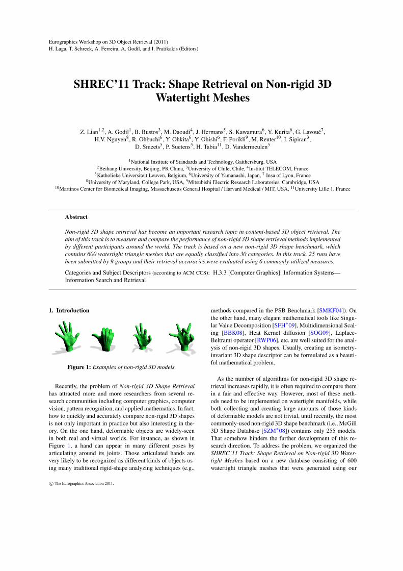
Figure 1: Examples of non-rigid 3D models.

Recently, the problem of Non-rigid 3D Shape Retrievalhas attracted more and more researchers from several re-search communities including computer graphics, computervision, pattern recognition, and applied mathematics. In fact,how to quickly and accurately compare non-rigid 3D shapesis not only important in practice but also interesting in the-ory. On the one hand, deformable objects are widely-seenin both real and virtual worlds. For instance, as shown inFigure 1, a hand can appear in many different poses byarticulating around its joints. Those articulated hands arevery likely to be recognized as different kinds of objects us-ing many traditional rigid-shape analyzing techniques (e.g.,

methods compared in the PSB Benchmark [SMKF04]). Onthe other hand, many elegant mathematical tools like Singu-lar Value Decomposition [SFH∗09], Multidimensional Scal-ing [BBK08], Heat Kernel diffusion [SOG09], Laplace-Beltrami operator [RWP06], etc. are well suited for the anal-ysis of non-rigid 3D shapes. Usually, creating an isometry-invariant 3D shape descriptor can be formulated as a beauti-ful mathematical problem.

As the number of algorithms for non-rigid 3D shape re-trieval increases rapidly, it is often required to compare themin a fair and effective way. However, most of these meth-ods need to be implemented on watertight manifolds, whileboth collecting and creating large amounts of those kindsof deformable models are not trivial, until recently, the mostcommonly-used non-rigid 3D shape benchmark (i.e., McGill3D Shape Database [SZM∗08]) contains only 255 models.That somehow hinders the further development of this re-search direction. To address the problem, we organized theSHREC’11 Track: Shape Retrieval on Non-rigid 3D Water-tight Meshes based on a new database consisting of 600watertight triangle meshes that were generated using our

c© The Eurographics Association 2011.

Z. Lian et al. / SHREC’11 Track: Shape Retrieval on Non-rigid 3D Watertight Meshes

own program as well as several commercial 3D modelingsoftware. In this track, we asked each participant to sub-mit up to five distance matrices obtained using their methodswithin one week. Finally, 25 matrices have been submittedby 9 groups and their retrieval accuracies were evaluated andcompared based on 6 standard measures.

2. Data Collection

The new database used in this track contains 600 watertighttriangle meshes that are derived from 30 original models,among which 26 objects are collected from several freely-accessible repositories (e.g., PSB database [SMKF04],McGill database [SZM∗08], TOSCA shapes [BBK08], etc.)while the other 4 models (i.e., lamp, paper, scissor, andtwoballs) are created by us using Autodesk 3d Max. Givena 3D mesh, we use Autodesk 3d Max to build its skeletonand then generate 19 deformed versions of the mesh by ar-ticulating around its joints in different ways. To remove theinner structures of those articulated models, we implementour own codes to first capture 18 depth-buffer views for thenormalized object on the vertices of a unit geodesic sphere,and then convert those images into a point cloud. Finally, wewrap the point cloud into a polygon surface and fix it to forma watertight 3D manifold without any topological errors byusing Geomagic, which can be automatically implementedwith recorded macros. As shown in Figure 2, those 600 non-rigid models have been equally classified into 30 categories.

3. Evaluation

Participants are asked to test their algorithms on the databaseto compute the dissimilarity between every two objects, andthen generate a distance matrix for each method. The matrixis composed of 600×600 floating point numbers, where thenumber at position (i, j) represents the dissimilarity betweenmodels i and j.

Analyzing the matrices submitted by participants, weevaluate their retrieval performance based on Precision-recall curves as well as the following five quantitativemeasures (see [SMKF04] for detailed definitions): Near-est Neighbor (NN), First Tier (FT), Second Tier (ST), E-measure (E), and Discounted Cumulative Gain (DCG).

4. Participants

This year, we have 9 groups taking part in the SHREC’11Track: Shape Retrieval on Non-rigid 3D Watertight Meshesand, totally, 25 dissimilarity matrices have been submitted.

1. FOG, FOG+MR and FOG+MRR submitted by ShunKawamura, Yukinori Kurita and Ryutarou Ohbuchi fromUniversity of Yamanashi, Japan.

2. T-NoNorm-40Coef, T-r01-40Coef, T-r01-50Coef, T-r015-40Coef and T-r015-50Coef submitted by GuillaumeLavoué from Insa of Lyon, France

3. MDS-CM-BOF submitted by Zhouhui Lian and AfzalGodil from National Institute of Standards and Technol-ogy, USA.

4. BOGH submitted by Hien Van Nguyen from Universityof Maryland, College Park, USA and Fatih Porikli fromMitsubishi Electric Research Laboratories, USA.

5. LSF and MLSF submitted by Yuki Ohkita, Yuya Ohishi,Shun Kawamura and Ryutarou Ohbuchi from Universityof Yamanashi, Japan.

6. ShapeDNA: OrigM-n10-norm1, OrigM-n12-norm1,OrigM-n12-normA, OrigM-n15-norm1 and ReM-n12-norm1 submitted by Martin Reuter from MartinosCenter for Biomedical Imaging, Massachusetts GeneralHospital / Harvard Medical / MIT, USA.

7. Harris3DGeoMap16, Harris3DGeoMap32 and HKSsubmitted by Ivan Sipiran and Benjamin Bustos fromUniversity of Chile, Chile.

8. MeshSIFT, SD-GDM and SD-GDM-meshSIFT submit-ted by Dirk Smeets, Jeroen Hermans, Dirk Vandermeulenand Paul Suetens from Katholieke Universiteit Leuven,Belgium.

9. PatchBOF_100 and PatchBOF_150 submitted by HediTabia from University Lille 1, France and MohamedDaoudi from Institut TELECOM, France.

5. Methods

5.1. Features on Geodesics (FoG), by S. Kawamura, Y.Kurita and R. Ohbuchi

The Features on Geodesics (FoG) algorithm is based on adiffusion-like distance on 3D mesh surface to achieve ro-bustness against articulation. In addition, the FoG is de-signed to accept diverse surface-based 3D models, e.g., non-watertight mesh or polygon-soup.

To compute features, the FoG method first resamples thesurface of a model by uniformly and quasi-randomly gen-erating Nsp oriented points (Nsp ≈ 3000). These points arethen reconstructed into a mesh by using k-nearest neighborconnectivity. This remeshing gains invariances to shape rep-resentation and tessellation, in exchange for retrieval accu-racy.

After remeshing, the algorithm computes a set of local-FoG features at Nk (Nk ≈ 500) randomly-selected key-pointson the mesh by using the Manifold Ranking algorithm de-veloped by Zhou et al. [ZBL∗03]. The manifold ranking al-gorithm is originally designed to compute distances amongfeatures in high dimensional feature space. The k-nearestneighbor meshing in the feature space of the original mani-fold ranking algorithm is replaced with the mesh resamplingmentioned above.

For each key-point, a local-FoG is computed as a set ofgeodesic-like distances for vertices that lie within a radiusr sphere of interest (using 3D Euclidian distance). A local-FoG feature centered at the key-point captures local geome-



Figure 2: Examples of models in our database that is classified into 30 categories.

try at multiple scales, by having multiple radius of interest rand multiple parameters σ that controls the diffusion speedduring the computation of manifold ranking.

A histogram of these distances coupled with a local geo-metrical feature within the same sphere becomes the local-FoG feature at the key-point. A set of Nk local FoG featuresare integrated into a feature vector per 3D model by using thebag-of-words approach. For the FoG algorithm, Kullback-Leibler Divergence is used to compute distance between twofeatures. For the FoG-MR and FoG-MRR methods, simi-larity between features is computed by using the (original)Manifold Ranking algorithm. Using manifold ranking forfeature distance computation appears to improve high-recallretrieval performance at the expense of low-recall (e.g., near-est neighbor) retrieval performance.

5.2. Bag of Words with Local Spectral Descriptors, byG. Lavoué

The method is based on the Bag of Words (BoW) paradigm.In this method, a uniform sampling is first utilized to gener-ate feature points on the mesh surface; for this goal, a ran-dom set of np vertices on the mesh is considered as an initialset of seeds, and then Lloyd relaxation iterations are imple-mented. Lloyd’s algorithm [Llo82] is a fixed-point iterationthat simply consists of iteratively moving the seeds to thecentroids of their Voronoi cells. Each feature point pi is thenassociated with a local patch Pi on which a descriptor is cal-

culated. For each feature point, this local patch is extractedby considering the connected set of facets belonging to agiven sphere of center pi and of a given radius r.

After that, each feature point is associated to a descrip-tor computed on its patch. The Fourier spectra of the patchis computed by projecting the geometry onto the eigenvec-tors of the Laplace-Beltrami operator. The Laplace-Beltramioperator ∆ is the counterpart of the Laplace operator in Eu-clidian space. It is defined as the divergence of the gradi-ent for functions defined over manifolds. The eigenfunctionand eigenvalue pairs (Hk,λk) of this operator satisfy thefollowing relationships:−∆Hk = λkHk. In the case of a 2-manifold triangular mesh the above eigen-problem can bediscretized and simplified within the finite element model-ing framework [LZ10]:−Qhk = λkDhk, in which hk denotesthe vector [Hk

1 , ...Hkm] where m is the number of vertices of

the patch. D is the Lumped Mass matrix and Q is the Stiff-ness matrix. To resolve this discrete eigenproblem, the fastalgorithm from Vallet and Lévy [VL08], based on a band-by-band approach and an efficient eigen-solver, is adopted;hence the eigenvectors hk (i.e. the manifold harmonic bases)and the associated eigenvalues are obtained. The spectral co-efficients are then calculated as the inner product betweenthe geometry of the surface and the sorted eigenvectors. Forx (resp. y,z):

xk =< x,hk >=m

∑i=1

xiDi,iHki (1)



The kth (k = 1..m) spectral coefficient amplitude is then de-fined as:

ck =√

(xk)2 +(yk)2 +(zk)2 (2)

Thus, for a given patch Pi around a feature point pi, thedescriptor is the spectral amplitude vector ci = [ci

1, ...cinc ],

with cik, the kth spectral coefficient amplitude of the patch

Pi. Here, only the nc first spectral coefficients are consideredto limit the descriptor to low/medium frequencies.

Given a 3D object containing a set of patches Pi associ-ated with descriptors ci, the next step is to represent it as adistribution of visual words from a given dictionary. First,the visual dictionary is created by clustering a huge datasetof descriptors and keep the nw centroids ck of the clusters asvisual words. Then, each patch Pi is associated with its clos-est visual word and the bag of words bM of the whole modelM is a nw-dimensional vector containing the distribution ofthe visual words over all its patches. The matching betweentwo bags of words is simply done using the L1 distance.

For the track, settings of this algorithm are as follows:

• The size nw of the dictionary was set to 200 and the num-ber of patchs np was set to 200.

• The visual vocabulary was computed from the test set.• Four versions have been proposed by changing the size

of the patches (r = 10% and r = 15% of the boundingbox length) and by changing the number of spectral coef-ficients (nc = 40 and nc = 50). A supplementary versionis also tested where the radius of the patches is fixed tor = 0.15.

5.3. Visual Similarity based Non-rigid 3D ShapeRetrieval Using MDS, by Z. Lian and A. Godil

Figure 3: Procedures of the canonical form computation.

The method [LGSZ10] performs step by step as follows:

1) Canonical Form Computation: Calculate the canoni-cal form for a 3D model based on MDS and PCA. As shownin Figure 3, the least squares technique with the SAMCOFalgorithm is chosen to implement the MDS embedding (Fig-ure 3(c)), and before that the number of vertices on the meshhas been reduced to about 1000 (Figure 3(b)).

2) Local Feature Extraction: Capture 66 depth-bufferviews for the canonical form on the vertices of a givengeodesic sphere, and then extract salient SIFT descrip-tors [Low04] from these views (Figure 4).

3) Word Histogram Construction: Generate a word his-togram by vector quantizing each view’s local featuresagainst a pre-specified codebook, such that the shape canbe represented by a set of histograms. It should be pointedout that the codebook is built by using K-means to create256 clusters for large numbers of local features randomlysampled from MDS embedded McGill database, and a par-ticular data structure (Figure 4) is designed to represent thehistogram in a more efficient and effective way [LGS10].

4) Dissimilarity Calculation: Carry out an efficient multi-view shape matching (Clock Matching) scheme [LRS10] tomeasure the dissimilarity between two models by calculatingthe minimum distance of their 24 matching pairs.

Since the method is mainly based on Multidimen-sional Scaling, Clock Matching, and Bag-of-Features,for the sake of convenience, it is denoted as “MDS-CM-BOF”. More details of this method can be foundin [LGSZ10] [LGS10] [LRS10].

Figure 4: Represent a depth-buffer view as a word histogramby the vector quantization of its SIFT local features.

5.4. Bag of Geodesic Histograms, by H.V. Nguyen and F.Porikli

The method uses a Bag-of-Feature approach and NormalizedGeodesic Distances to retrieval non-rigid 3D shapes.

Consider a shape to be a closed set S ∈Rn. The geodesicdistance γ(p,q) between two points p and q is defined to bethe shortest path among all paths connecting these two pointson the shape. Let h(p) = [h1(p),h2(p), . . . ,hn(p)] denotesthe histogram of geodesic distances from the point p to allpoints in S, which is defined as follows:

hi(p) =Qi

S (3)

Qi =

{q ∈ S|(i−1)∆ ≤ γ(p,q)

γp≤ i∆

}(4)

where γp is the mean of geodesic distance from p to allpoints, and ∆ is the separation between histogram bins. Here,n = 100 and ∆ = 0.025. Since the descriptor is based on thegeodesic distances, they are robust to various 3D non-rigidarticulations. In addition, the normalization with respect toaverage geodesic distances take into account the scaling ef-fects.



For each shape, N points (here N = 300) are randomlychosen and a bag of descriptors is computed. Shape match-ing is done by first finding the optimal correspondences be-tween their bags of descriptors using the Hungarian algo-rithm.

Let two sets of the descriptors for two shapes A and B beΛ

A : hA1 ,hA

2 , ..hAN and Λ

B : hB1 ,hB

2 , ..hBN . The correspondence

is established through a one-to-one mapping function τ suchthat τ : Λ

A ↔ΛB. If a descriptor hA

i is matched to another hBi

then τ(iA) = jB and τ( jB) = iA. The cost function is definedas

E(h) = ∑1≤i≤N

ε(τ(i), i) (5)

where the distance between two descriptors is computed us-ing χ

2 statistic

ε(τ(i), i) = ∑1≤k≤N

[hAτ(i)(k)−hB

i (k)]2

hAτ(i)(k)+hB

i (k)(6)

Finally, the optimal cost E(h) is used as the similaritymeasure between two shapes.

5.5. Localized Statistical Features (LSF), by Y. Ohkita,Y. Ohishi, S. Kawamura and R. Ohbuchi

Figure 5: Localized Statistical Features (LSF).

The Localized Statistical Features (LSF) is a very sim-ple 3D shape descriptor that has a set of good robustnessproperties [OFO09]. The LSF is robust against shape rep-resentations; the LSF can handle 3D models represented aspolygon soup, oriented point set, watertight mesh, arwaterleakingas manifold mesh, etc. The LSF is robust against sim-ilarity transformation without requiring any pose normaliza-tion. It is also fairly robust against geometrical/topologicalnoise. Finally, the LSF is robust against articulation.

The LSF computes a set of Nk (Nk ≈ 500) localized3D statistical features, which are then combined into afeature vector per 3D model by using the bag-of-wordsapproach. Each statistical feature is a derivative of theSurflet-Pair-Relation Histograms (SPRH) feature by Wahl etal. [WHH03]. The SPRH feature accepts a 3D model in ori-ented point set representation. From the point set, the SPRH

computes a 4D joint histogram consisting of three angles (in-ner product, etc.) and a distance among all the pairs of theoriented points.

For the LSF, the SPRH descriptor is made to be local.Each LSF is computed from the point set within the sphereof radius r about the Nk keypoints quasi-randomly and uni-formly placed on the surfaces of the model. In LSF, his-togram is computed from point pairs in which one of thepoints is the keypoint. If there are n points in the sphere,there are (n− 1) pairs of points filling the histogram. In theMulti-resolution LSF (MLSF), multiple radii of influencesare used, in an attempt to capture multi-scale geometricalfeatures.

After the set of local features are computed, they are com-bined into a feature vector per 3D model by using the bag-of-features approach. Here, the LSF feature is used as is, i.e.,without Manifold Ranking and other distance metric learn-ing.

5.6. ShapeDNA: Laplace Spectra for Non-Rigid ShapeAnalysis, by M. Reuter

The ShapeDNA has been introduced in 2005 [RWP06] asthe first spectral method used for non-rigid shape analy-sis. Spectral methods have later been employed by the au-thors for local shape analysis of structures in the humanbrain to analyse disease effects [RWSN09] and for automaticshape segmentation [Reu10]. ShapeDNA is the normed be-ginning sequence of the spectrum (i.e. the first eigenvalues)of the Laplace-Beltrami operator (LBO) for 2D surfaces or3D solids. The eigenvalues λ and eigenfunctions u are thesolution of the Laplacian eigenvalue problem ∆u = −λu,where ∆u := div(grad(u)) with grad being the gradient anddiv the divergence with respect to the underlying domain orRiemannian manifold in general. The normed first smallestN eigenvalues 0 ≤ λ1 ≤ λ2 ≤ ... ≤ λn are employed as ashape descriptor (ShapeDNA). In addition to the isometryinvariance, the beginning sequence of the Laplace spectrahas many desirable properties. This descriptor is insensi-tive to noise, which influences mainly the higher eigenval-ues. Possible switching of eigenvalues is not problematic (asopposed to comparing eigenfunctions), as the values musthave been close to begin with. The spectrum can be com-pared easily and can be computed for many different shaperepresentations. It can deal with objects containing cavities(when using 3D solids), depends continuously on shape de-formations and can easily be made scaling invariant. Notethat the ShapeDNA does not rely on any prior knowledgeand opposed to other methods involving eigenfunctions orthe heat kernel, it yields a very simple and robust, isometryinvariant shape descriptor.

For this shape retrieval contest, the simple linear FEM isutilized to compute the first eigenvalues of the LBO. Sincefor shape retrieval only a small number of eigenvalues is



needed (usually less than 15) linear approaches should besufficient. Note that in order to compute a large number ofeigenvalues and eigenfunctions, maybe to approximate theheat kernel, higher order approximations are advisable, dueto their superior accuracy [RBG∗09].

For the ShapeDNA, several parameters can be modified.In addition to the FEM discretization, several parameters canbe specified. Earlier tests showed that usually N = 10 · · ·15eigenvalues are a good number (less have often not enoughpower to distinguish shapes, while including higher val-ues increases influence of noise and non-isometric deforma-tions).The first eigenvalue is omitted as it is zero for closedmanifolds. Another parameter is the distance metric to com-pare the spectra, where the simple Euclidean distance on theN dimensional vector of numbers is chosen. Finally, in orderto compare shape rather than size of the objects, the spectraneed to be normalized. One option is to multiply the spec-trum by the surface area (normA), which is the same as nor-malizing the area of the shapes before computation. Anotheroption is to divide the sequence by the first non-zero eigen-value (norm1), which is of course the same in the perfect iso-metric cases. However, shapes are usually not perfectly iso-metric and dividing by the first non-zero eigenvalue can helpto identify similar shapes in spite of noise or near-isometricdeformations. As sometimes mesh quality can degrade theaccuracy especially of the linearly approximated eigenval-ues, the ShapeDNA is also computed on remeshed (ReM)shapes, in addition to the original meshes (OrigM).

Software to compute eigenvalues and vectors of theLaplace-Beltrami operator with up to cubic FEM on trianglemeshes is freely available for non-profit research at [Reu].

5.7. Keypoints-based matching of non-rigid shapes, byI. Sipiran and B. Bustos

This section presents two techniques, including Harris 3Dand Heat Kernel Signatures methods, to tackle the problemof non-rigid 3D shape retrieval.

5.7.1. Harris 3D Geodesic Map

The idea behind this method is to compute a characteristicdistribution of geodesic distances between the interest pointsof a shape. So the method starts by detecting interest pointsof a shape using the Harris 3D method [SB]. For this track,adaptive neighborhoods with δ = 0.01 are utilized and the0.01% of the number of vertices with the highest Harris re-sponse are selected as interest points.

Let F be the set of interest points detected. The com-plete set of geodesic distances between each pair of inter-est points is computed. This set is represented by the ma-trix D of dimension |F|× |F|. Values in the matrix are nor-malized through dividing each entry by the maximum value.This makes the values invariant against scale.

Next, a histogram is created with n bins, which divides

the interval [0,1] of possible normalized geodesic distances.Then, m samples are randomly selected from the matrixD, accumulating a vote in their corresponding bin. For thistrack, two configurations are chosen to compute the his-tograms: 1) n = 16, m = 1000; 2) n = 32, m = 2000. Thedistance between two histograms is measured using the Eu-clidean distance.

5.7.2. HKS based Point-to-point Matching

Heat kernel signatures method (HKS) [SOG09] has provento be an interesting mesh analysis tool. Unlike Harris 3D,HKS computes a descriptor for each vertex on a mesh. Thesedescriptors are invariant to non-rigid transformations, allow-ing to detect interest points too.

The method starts by detecting the interest points usingthe Heat kernel signatures. For this track, descriptors oflength 100 are used and t = 0.1 of the area of the surface isconsidered as the value for comparing the HKS for interestpoint detection. Once the interest points have been detected,each interest point has an associated HKS descriptor. Then,a shape is represented by a set of HKS descriptors associatedto the interest points.

As HKS is based on an intrinsic formulation of a mesh,the descriptors are expected to be very similar in pres-ence of non-rigid transformations. Based on this fact, theset of descriptors of two shapes are compared. Let S ={s1,s2, · · · ,sn} and P = {p1, p2, · · · ,sm} be the sets of de-scriptors of two shapes. The dissimilarity between S and Pis defined as

d(S,P) = ∑nk=1 dmin(sk,P)

n(7)

where

dmin(si,P) = mins j∈P

‖si− s j‖2 (8)

5.8. Fusion of SD-GDM and meshSIFT, by D. Smeets, J.Hermans, D. Vandermeulen and P. Suetens

The method combines a global feature method (SD-GDM)with a local features method (meshSIFT) for non-rigid 3Dshape retrieval.

5.8.1. Spectral Decomposition of the Geodesic DistanceMatrix (SD-GDM)

For the SD-GDM approach [SFH∗09], 3D shapes are repre-sented by a geodesic distance matrix (GDM), which is a iso-metric deformation invariant matrix. It contains the geodesicdistance between each pair of points on the surface.

As preprocessing, the surface meshes are first down-sampled to about 2500 points. Geodesic distances are thencalculated with a fast marching algorithm for triangulatedmeshes [PC09]. To compensate for scale differences in the



3D shapes, the geodesic distances are normalized by thesquare root of the total surface area.

Next, spectral decomposition (SD) of the GDM providesa sampling order invariant global feature (shape descriptor).In [SFH∗09], it is proved that the modal representation, i.e.,the eigenvalue matrix, is invariant to the sampling order un-der the condition that each point on one surface has one cor-responding point on the other surface, which can be assumedfor watertight meshes after resampling. Object recognitionreduces to direct comparison of the shape descriptors with-out the need to establish explicit point correspondences. Forcomputational reasons, only the 40 largest eigenvalues arecalculated. The modal representations of the GDMs are thencompared using the mean normalized Manhattan distance asin [SFH∗09].

5.8.2. Scale Invariant Feature Transform for meshes(meshSIFT)

Similar to the scale invariant feature transform (SIFT) al-gorithm [Low04], the meshSIFT algorithm consists of threemajor components: keypoints detection, orientations assign-ment and a local feature descriptor [MFK∗10].

The algorithm first detects scale space extrema as localfeature locations. The scale space contains the mean curva-ture in each vertex on different smoothed versions of the in-put mesh. Smoothing consists of subsequent convolutions ofthe mesh with a binomial filter.

In order to have an orientation-invariant descriptor, eachkeypoint is assigned a canonical orientation. Therefore thenormal vectors in the neighborhood of each keypoint areprojected onto the tangent plane. The canonical orientationis the most frequently occurring orientation in the tangentplane (more details in [MFK∗10]).

The meshSIFT algorithm then describes the neighbour-hood of every scale space extremum in a feature vector con-sisting of concatenated histograms of shape indices and slantangles. The 144D feature vectors are matched by comparingthe angle in feature space. If the ratio between the first andthe second smallest angle is smaller than 0.9, a match is ac-cepted; other matches are rejected. Finally, the number ofmatches is used as similarity between two shapes. The simi-larity matrix is converted into a dissimilarity matrix by sub-tracting the matrix from the maximum number of matches.

5.8.3. Fusion (SD-GDM-meshSIFT)

To combine the SD-GDM approach with the meshSIFT ap-proach, the corresponding dissimilarity matrices are firstnormalized using min-max normalization. Finally they arefused using the sum rule.

5.9. Bag-of Densely-Sampled Local Visual Features, byH. Tabia and M. Daoudi

The method consists of the following four steps(see [TDVC11] for more details):

1) Detection and description of 3D patches: Let v1 andv2 be the farthest vertices (in the geodesic sense) on a con-nected triangulated surface S. Let f1 and f2 be two scalarfunctions defined on each vertex v of the surface S, as fol-lows: f1(v) = d(v,v1) and f2(v) = d(v,v2) where d(x,y) isthe geodesic distance between points x and y on the surface.In a critical point classification, a local minimum of fi(v)is defined as a vertex vmin such that all its level-one neigh-bors have a higher function value. While, a local maximumis a vertex vmax such that all its level-one neighbors havea lower function value. Let F1 be the set of local extrema(minima and maxima) of f1 and F2 be the set of local ex-trema of f2. The set of feature points F of the triangulatedsurface S is defined as the closest intersecting points in thesets F1 and F2. Given a 3D object O, for every feature pointFi ∈ F , a descriptor P(Fi) is defined for Fi and the geodesicdistances {d(Fi,v);∀v ∈ V} with V is the set of all verticeson the surface are calculated. Consider f the distribution ofvertices according to these distances, the descriptor P(Fi)is defined as a R-dimensional vector: P(Fi) = (p1, . . . , pR)where pr =

∫ r/R(r−1)/R f (d)δd. P(Fi) is a R-bin histogram of

vertex distribution of geodesic distances measured from Fi.In order to make the descriptors comparable between differ-ent shapes, the geodesic function d is scaled by the geodesicdiameter of the shape.

2) Shape vocabulary construction: The vocabulary usedin this method is a way of constructing a feature vector thatrelates descriptors in 3D-object query to descriptors previ-ously seen in the indexing step. The k-means algorithm ischosen for clustering. In order to determine the parameterk, the k-means method is implemented several times withdifferent number of desired k, and then the final clusteringgiving the lowest empirical risk is selected.

3) Shape histogram computing: Descriptors in the 3D ob-ject are assigned to the nearest neighbor keyshapes in the vo-cabulary. Then each object is represented using an histogramwhose ith bin contains the number of ith keyshapes in thatobject.

4) Shape matching: Compare two objects, treating theirbag of keyshapes as feature vectors, and thus determine theirdissimilarity by calculating L2 difference between two his-tograms.

6. Results

This section presents and compares the results of 25 runssubmitted by 9 groups. Given the 25 dissimilarity matrices,we carry out evaluations for these methods not only on theaverage performance of the whole database, but also on the



Table 1: Retrieval performance of all runs evaluated usingfive standard measures on the whole database.

result corresponding to each specific class. The evaluationmeasures used here are the five quantitative statistics (i.e.NN, FT, ST, E, and DCG) and the Precision-recall curvesmentioned in Section 3.

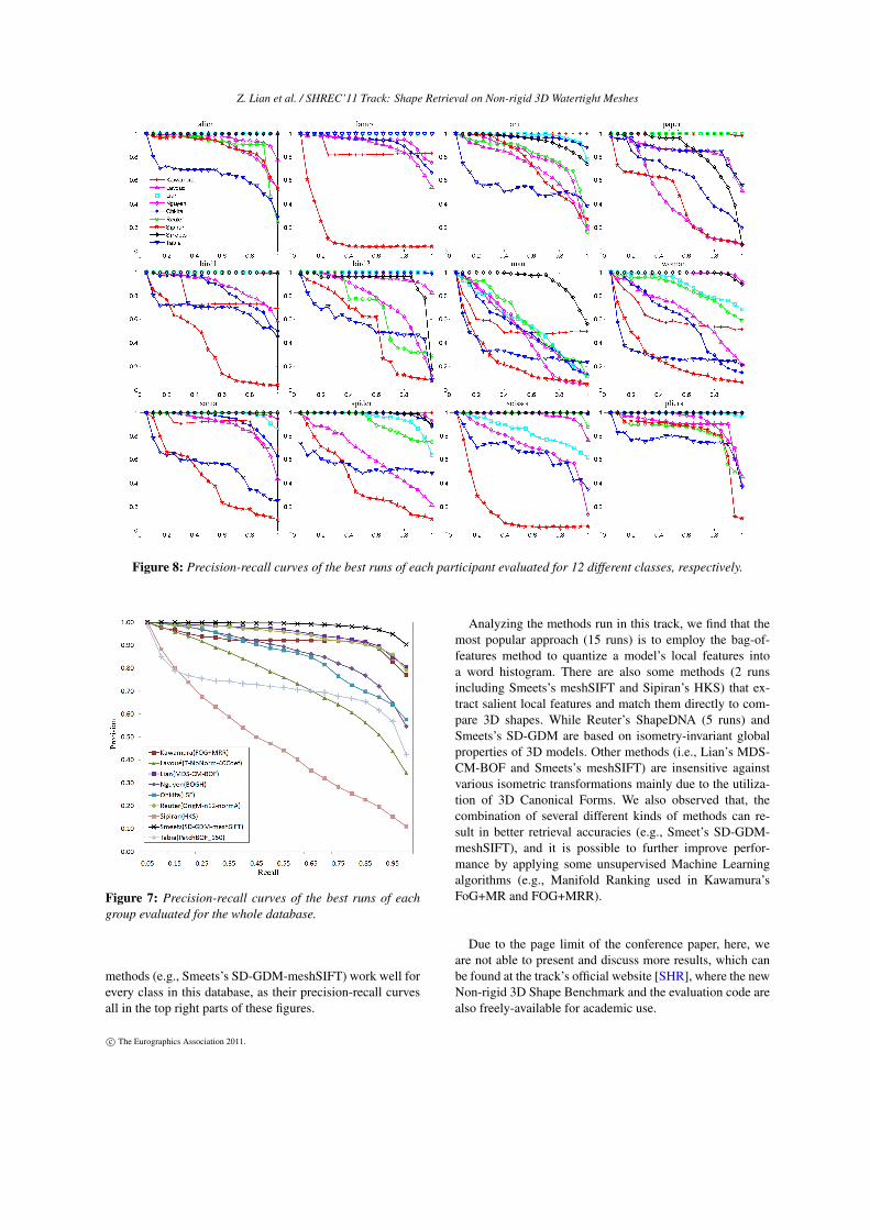
Table 1 lists the retrieval accuracies of all 25 methods(or methods with different settings) evaluated on the wholedatabase. We observe that most of these methods performwell in this track. For example, DCG values of 15 runs aregreater than 0.940 and 20 runs have NN values that are above0.950. In Figure 6, we also provide column charts to intu-itively compare the best results of each group evaluated us-ing five quantitative measures, respectively. As we can seefrom Figure 6, Smeets’s SD-GDM-meshSIFT clearly out-performs all other algorithms, while the second and thirdbest methods are not so obvious. Considering the values ofNN and FT, Reuter’s methods get better performance thanLian’s, but if we base the evaluation on ST, E, and DCG,Lian’s MDS-CM-BOF would take the second place. Simi-lar observations can be made from Figure 7, which showsPrecision-recall curves of the best runs submitted by eachgroup on the whole database.

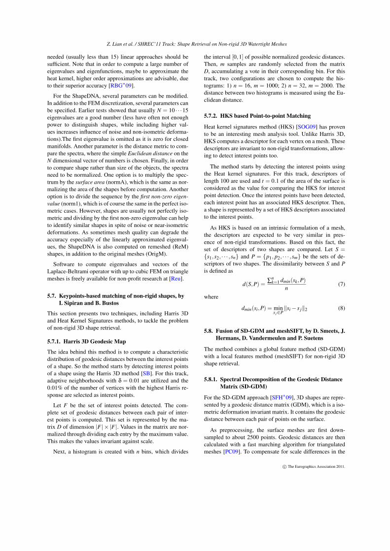
Figure 8 shows the Precision-recall curves of the bestruns of each group measured for selected 12 classes in thenon-rigid database. We find that none of these methods per-forms best for all kinds of objects. For instance, Smeets’sSD-GDM-meshSIFT obtains the best results when searching

Figure 6: Column charts of the best retrieval accuracies ofeach group evaluated on the whole database using five stan-dard measures, respectively.

for lots of categories but not ant, paper, spider models, etc.,while although Tabia’s PatchBOF_150 performs worst inthe retrieval of alien models, it outperforms others for lampmodels. As shown in Figure 2, our database contains a set ofmodels which have similar overall appearances but belongto various categories because they are different in the detailsof local regions or/and topological structures. This makesthe new benchmark more challenging than other non-rigid3D databases. However, as we can see from Figure 8, thechallenge can be well resolved by several algorithms used inthis track. For example, Lian’s MDS-CM-BOF are able toperfectly discriminate two types of bird models (i.e., bird1and bird2), which have slightly different skeletons, whileSmeets’s SD-GDM-meshSIFT obtains considerably high re-trieval accuracies for the bird models as well as the humanmodels (i.e., man and woman) that possess dissimilar fea-tures based on gender. Generally speaking, most of these



Figure 8: Precision-recall curves of the best runs of each participant evaluated for 12 different classes, respectively.

Figure 7: Precision-recall curves of the best runs of eachgroup evaluated for the whole database.

methods (e.g., Smeets’s SD-GDM-meshSIFT) work well forevery class in this database, as their precision-recall curvesall in the top right parts of these figures.

Analyzing the methods run in this track, we find that themost popular approach (15 runs) is to employ the bag-of-features method to quantize a model’s local features intoa word histogram. There are also some methods (2 runsincluding Smeets’s meshSIFT and Sipiran’s HKS) that ex-tract salient local features and match them directly to com-pare 3D shapes. While Reuter’s ShapeDNA (5 runs) andSmeets’s SD-GDM are based on isometry-invariant globalproperties of 3D models. Other methods (i.e., Lian’s MDS-CM-BOF and Smeets’s meshSIFT) are insensitive againstvarious isometric transformations mainly due to the utiliza-tion of 3D Canonical Forms. We also observed that, thecombination of several different kinds of methods can re-sult in better retrieval accuracies (e.g., Smeet’s SD-GDM-meshSIFT), and it is possible to further improve perfor-mance by applying some unsupervised Machine Learningalgorithms (e.g., Manifold Ranking used in Kawamura’sFoG+MR and FOG+MRR).

Due to the page limit of the conference paper, here, weare not able to present and discuss more results, which canbe found at the track’s official website [SHR], where the newNon-rigid 3D Shape Benchmark and the evaluation code arealso freely-available for academic use.



7. Conclusion

In this paper, we first presented the background of non-rigid3D shape retrieval. Next, we mentioned how to construct thenew database and how to evaluate retrieval performance forthe SHREC’11 Track: Shape Retrieval on Non-rigid 3D Wa-tertight Meshes. Afterwards, we briefly described all meth-ods (25 runs) used by 9 groups who successfully participatedin this track. Finally, experimental results were presented tocompare the effectiveness of different algorithms.

The non-rigid track organized this year is the secondattempt in the history of SHREC to specifically focuson the performance evaluation of non-rigid 3D shape re-trieval algorithms. Compared to the first non-rigid SHRECtrack [LGF∗] (200 models and 3 groups) we organized in2010, both the size of database (600 models) and the numberof participants (9 groups) tripled this year, which indicatesthat more and more researchers have become interested inanalyzing non-rigid 3D shapes. We believe that, with such alarge number of participants taking part in the track, meth-ods described in this paper most likely represent the state-of-the-art in this important research direction, and we hope thatthe new benchmark will further promote the investigation ofnon-rigid 3D shape retrieval.

Disclaimer

Any mention of commercial products or reference to com-mercial organizations is for information only; it does notimply recommendation or endorsement by NIST nor doesit imply that the products mentioned are necessarily the bestavailable for the purpose.

ACKNOWLEDGMENTS

This work has been supported by the SIMA programand the Shape Metrology IMS. We would like to thankAIM@SHAPE, Cyberware, Kaleem Siddiqi, Philip Shilane,Michael Bronstein, Robert Sumner, and Daniela Giorgi forproviding original 3D models.

References[BBK08] BRONSTEIN A. M., BRONSTEIN M. M., KIMMEL R.:

Numerical geometry of non-rigid shapes. Springer, 2008.

[LGF∗] LIAN Z., GODIL A., FABRY T., FURUYA T., HERMANSJ., OHBUCHI R., SHU C., SMEETS D., SUETENS P., VANDER-MEULEN D., WUHRER S.: SHREC’10 Track: Non-rigid 3DShape Retrieval. In Proc. 3DOR’10, pp. 101–108.

[LGS10] LIAN Z., GODIL A., SUN X.: Visual similarity based3D shape retrieval using bag-of-features. In Proc. SMI’10 (2010),pp. 25–36.

[LGSZ10] LIAN Z., GODIL A., SUN X., ZHANG H.: Non-rigid3D shape retrieval using multidimensional scaling and bag-of-features. In Proc. ICIP 2010 (2010), pp. 3181–3184.

[Llo82] LLOYD S.: Least squares quantization in PCM. IEEETrans. Information Theory 28, 2 (1982), 129–137.

[Low04] LOWE D. G.: Distinctive image features from scale-invariant keypoints. IJCV 60, 2 (2004), 91–110.

[LRS10] LIAN Z., ROSIN P. L., SUN X.: Rectilinearity of 3Dmeshes. IJCV 89, 2-3 (2010), 130–151.

[LZ10] LÉVY B., ZHANG H.: Spectral mesh processing. Sig-graph 2010 Course (2010).

[MFK∗10] MAES C., FABRY T., KEUSTERMANS J., SMEETSD., SUETENS P., VANDERMEULEN D.: Feature detection on 3Dface surfaces for pose normalisation and recognition. In Proc.BTAS’10 (2010).

[OFO09] OHKITA Y., FURUYA T., OHBUCHI R.: Sets of local3d shape descriptors for 3d model retrieval. In Proc. Visual Com-puting Symposium 2009 (in Japanese) (2009).

[PC09] PEYRÉ G., COHEN L. D.: Heuristically Driven FrontPropagation for Fast Geodesic Extraction. IJVCB 1, 1 (2009),55–67.

[RBG∗09] REUTER M., BIASOTTI S., GIORGI D., PATANÈ G.,SPAGNUOLO M.: Discrete Laplace-Beltrami operators for shapeanalysis and segmentation. Computers & Graphics 33, 3 (2009),381–390.

[Reu] http://reuter.mit.edu/software.

[Reu10] REUTER M.: Hierarchical shape segmentation and reg-istration via topological features of Laplace-Beltrami eigenfunc-tions. IJCV 89, 2 (2010), 287–308.

[RWP06] REUTER M., WOLTER F. E., PEINECKE N.: Laplace-Beltrami spectra as shape-DNA of surfaces and solids.Computer-Aided Design 38, 4 (2006), 342–366.

[RWSN09] REUTER M., WOLTER F. E., SHENTON M., NI-ETHAMMER M.: Laplace-Beltrami eigenvalues and topolog-ical features of eigenfunctions for statistical shape analysis.Computer-Aided Design 41, 10 (2009), 739–755.

[SB] SIPIRAN I., BUSTOS B.: A robust 3D interest points detec-tor based on Harris operator. In Proc. 3DOR’10, pp. 7–14.

[SFH∗09] SMEETS D., FABRY T., HERMANS J., VANDER-MEULEN D., SUETENS P.: Isometric Deformation Modellingfor Object Recognition. In Proc. CAIP’09 (2009), pp. 757–765.

[SHR] http://www.itl.nist.gov/iad/vug/sharp/contest/2011/NonRigid/.

[SMKF04] SHILANE P., MIN P., KAZHDAN M., FUNKHOUSERT.: The princeton shape benchmark. In Proc. SMI’04 (2004),pp. 167–178.

[SOG09] SUN J., OVSJANIKOV M., GUIBAS L. J.: A Conciseand Provably Informative Multi-Scale Signature Based on HeatDiffusion. Comput. Graph. Forum 28, 5 (2009), 1383–1392.

[SZM∗08] SIDDIQI K., ZHANG J., MAXRINI D., SHOKOUFAN-DEH A., BOUIX S., DICKINSON S.: Retrieving articulated 3dmodels using medial surfaces. Machine Vision and Applications19, 4 (2008), 261–274.

[TDVC11] TABIA H., DAOUDI M., VANDEBORREB J. P.,COLOT O.: Deformable Shape Retrieval Using Bag-of-FeautreTechniques. In Proc. 3DIP’11 (2011).

[VL08] VALLET B., LÉVY B.: Spectral geometry processingwith manifold harmonics. Computer Graphics Forum 27, 2(2008), 251–260.

[WHH03] WAHL E., HILLENBRAND U., HIRZINGER G.:Surflet-Pair-Relation Histograms: A Statistical 3D-Shape Rep-resentation for Rapid Classification. In Proc. 3DIM’03 (2003),pp. 474–481.

[ZBL∗03] ZHOU D., BOUSQUET O., LAL T. N., WESTON J.,SCHÖLKOPF B.: Learning with local and global consistency. InProc. NIPS’03 (2003).


http://reuter.mit.edu/software

http://www.itl.nist.gov/iad/vug/sharp/contest/2011/NonRigid/

shrec’11 track: shape retrieval on non-rigid 3d …€™11 track: shape retrieval on non ......

Documents