Attachment 2 to BSCP32/4.1 Application for a Metering Dispensation

London Array Offshore Transmission Losses EJ/17th August 2011rev1 Relied Upon Information clarified. Revised cable lengths. NGET 400 kV recordings incorporated

The London Array has been designed and built to offshore grid connection standards, with settlement metering offshore, at its 33 kV Grid Entry Points.

During an initial operational period, prior to the relevant Transmission Licensee having adopted its offshore transmission asset, the wind farm will however be operated as a generator connected directly to the onshore 400 kV Interface Point, at which point no meters have been installed. A formula for calculating onshore power as a function of offshore meter reading is hence needed for that period.

The purpose of rhis Mathcad spreadsheet is to provide a such formula. By detailed loadflow, it models the offshore transmission system of one of the four London Array systems, from and including the offshore Grid Entry Point to and including the onshore Interface Point. Independent variables are power to the Grid Entry Point and the 400 kV voltage, so as to alow for varying Mvar loading; the voltage component is averaged out using a statistical approach.

The four systems are virtually identical. Hence, only one formula applicable to any of them is developed. Average component data and cable lengths are used.

150 kV

33 kV

SGT1A

GT1

HPPP1

SVC

MSR

Grid Entry Point

EXPO

RT C

ABLE

1

harmonicfilter

NGET1

2

3 (fictitious, y-equivalent)

4

5

6

7

8

9

to SGT1B

Single systemto which the

formula applies

MWh MWh

Blue: Node numbersapplied in the calculations

ResultAt a sum offshore meter readings Poffshore, the equivalent onshore power at 400 kV is:

Ponshore Poffshore( ) Poffshore 0.4334 2.6705 10 4 Poffshore2

[MWh per ½ h], MWh per ½ h]

Both Ponshore and Poffshore are in [MWh per ½ h].

Page 1 of 29

Relied upon information

Export cable lengths: VSGM-LAL-RP-3007_D - Export Cable Route Engineering_Report1.Export cable impedance and capacitance parameters: 27398-ETX-RT-21693_R3_Design_Report_-_Export_Cables2.Transformer losses: IEC routine test reports test certificate D417 120, test certificate D417 121, Test Report 01210, Test Report 1410, Test Report 3.180-2 (SGT 2A), Test Report 180-4 (SGT 2B)SVC: Email of Siemens Erlangen 110304_Losses_to_STDL with attached spreadsheet4.Onshore substation auxiliary supply: STDL G85221-W0047-V1-N001_N15.Harmonic filters: emai lJohn Finn 26th May 2011 and attachments Siemens Final Electric Test Report RE 059-11 and TC-92100871-010000 6.400 kV cable length: STDL data submission of 28.02.2011 for NGET User Data File, sheet LA Part 3 Section 2.1 Branch Data v2: LAL 1: 0.08 7.km;LAL 2 0.13 km400 kV voltage recordings, for assessing SVC losses: email Richard Lavender, NGET, 16th Aug 2011, with attached Volts Apr 11.zip 8.

Page 2 of 29

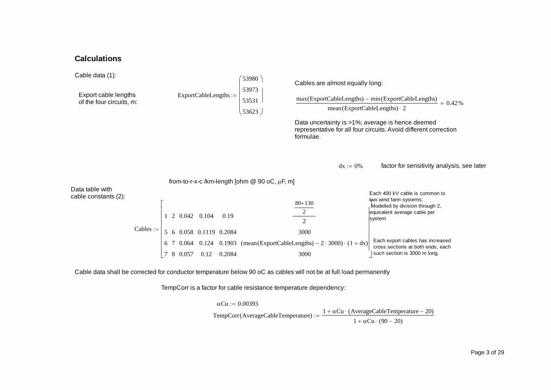
TempCorr AverageCableTemperature( )1 Cu AverageCableTemperature 20( )

1 Cu 90 20( )

Cu 0.00393

TempCorr is a factor for cable resistance temperature dependency:

Cable data shall be corrected for conductor temperature below 90 oC as cables will not be at full load permanently

Each export cables has increased cross sections at both ends, each such section is 3000 m long.

Cables

1

5

6

7

2

6

7

8

0.042

0.058

0.064

0.057

0.104

0.1119

0.124

0.12

0.19

0.2084

0.1903

0.2084

80 13022

3000

mean ExportCableLengths( ) 2 3000( ) 1 dx( )

3000

Each 400 kV cable is common to two wind farm systems. Modelled by division through 2, equivalent average cable per system

Data table withcable constants (2):

from-to-r-x-c /km-length [ohm @ 90 oC, F, m]

factor for sensitivity analysis, see laterdx 0%

Data uncertainty is >1%; average is hence deemed representative for all four circuits. Avoid different correction formulae.

max ExportCableLengths( ) min ExportCableLengths( )mean ExportCableLengths( ) 2

0.42%ExportCableLengths

53980

53973

53531

53623

Export cable lengthsof the four circuits, m:

Cables are almost equally long:Cable data (1):

Calculations

Page 3 of 29

The average cable temperature over a year will depend on the average ambient temperature and the average load as follows,conservatively assuming the cables to be designed to their limit conductor temperature 90 oC at maximum generation:

AverageCableTemperature90 AmbientTemperature( ) AveragePower2

TempCorr AverageCableTemperature( )AmbientTemperature=

Now find the annual average power from the wind turbine power curve and the statistical wind distribution:

Wind turbine power curve, SWT3.6@0.69 kV generator terminals, 1st row wind m/s 2nd relative power:

Pcrv3

0

4

0.022

5

0.066

6

0.132

7

0.223

8

0.343

9

0.492

10

0.661

11

0.819

12

0.926

13

0.976

14

0.994

15

0.998

16

1

17

1

18

1

19

1

20

1

21

1

22

1

23

1

24

1

25

1

T

-interpolate:pTurb v( ) 0 v Pcrv1 1if

0 v Pcrvrows Pcrv( ) 1if

i floor v( ) Pcrv1 1 1

Pcrvi 2Pcrvi 1 2 Pcrvi 2

Pcrvi 1 1 Pcrvi 1v Pcrvi 1

otherwise

Weibull wind distribution, wind speed probability density function:

2.4

9.33

Weibull v( )

v

1 e

v

Page 4 of 29

AveragePower0

25vpTurb v( ) Weibull v( )

d AveragePower 43.05%

The average ambient temperature of the sea bed will not be more than 12 deg C over a year.: AmbientTemperature 12

Solve the above nonlinear equation: Seed AverageCableTemperature 50

Given

AverageCableTemperature90 AmbientTemperature( ) AveragePower2

TempCorr AverageCableTemperature( )AmbientTemperature=

Find AverageCableTemperature( ) 29.75

However, this note takes the cautious approach of working with a higher temperature:

AverageCableTemperature 40

thereby overestimating the losses slightly:. TempCorr AverageCableTemperature( )TempCorr 29.75( )

1 3.88%

Do the correction:

Cables 3 TempCorr AverageCableTemperature( ) Cables 3

Page 5 of 29

Transformers (3):

from - to -kVprim -kVsec - baseMVA -ex - er - iMagn - noloadLoss% - AVRtarget -tapdist -tapDeadband

Onshore autotransformer with tertiary modelled by three fictitious two-winding transformers, first 3 rowsTrf

2

3

3

8

3

4

5

9

400

400

400

150

400

13.9

150

33

180

180

180

180

8.69 %

35.28%

20.28%

11.83%

0.061%

0.033%

0.122%

0.225%

0.074%

0

0

0.06%

0.036%

0

0

0.043%

0

0

103%

100%

0

0

1.25%

1.25%

0

0

2%

2%

Transformers could equally be subject to average temperature compensation, however not done as losses are modest. Data apply to full load and are hence conservative.

Shunt elements (6): at kVrated, Mvar rated positive = capacitor, MW losses

Harmonic filter, 20 Mvar, series reactorloss 0.432 plus dielectric loss 0.0585 W/kvar

Shunt 5 150 20 0.4320720150

2 0.0585 20 103

10 6

Page 6 of 29

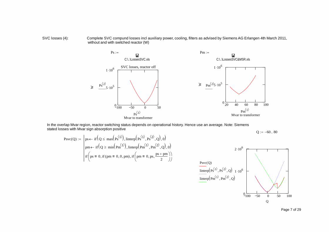
SVC losses (4): Complete SVC compund losses incl auxiliary power, cooling, filters as advised by Siemens AG Erlangen 4th March 2011, without and with switched reactor (W)

Ps

C:\..\LossesSVC.xls

Pm

C:\..\LossesSVC&MSR.xls

100 50 0 500

5 105

1 106 SVC losses, reactor off

Mvar to transformer

W

Ps 2

Ps 1

20 40 60 80 1000

5 105

1 106

Mvar to transformer

W Pm 2

Pm 1

In the overlap Mvar region, reactor switching status depends on operational history. Hence use an average. Note: Siemens stated losses with Mvar sign absorption positive

Q 60 80

Psvc Q( ) ps if Q max Ps 1 linterp Ps 1 Ps 2 Q 0

pm if Q min Pm 1 linterp Pm 1 Pm 2 Q 0

if ps 0= if pm 0= 0 pm( ) if pm 0= psps pm

2

100 50 0 50 1000

1 106

2 106

Psvc Q( )

linterp Ps 1 Ps 2 Q linterp Pm 1 Pm 2 Q

Q

Page 7 of 29

Substation load, per SGT section i.e. per Power Park Module MW (5).Note that SVC loads are to be subtracted as those have been included in the above SVC losses. Conservatively assume LV installation to be at dimensioning load at all times

PonshoreAux 184.1 10 3 Offshore substation load not to be

included as it is Generator metered.

Network calculation formulae

Vector of nodal powers as a function of relative MW generationand SVC reactive generation. Generator sign

Nominal voltages

pRel = power relative to installed turbine power PmaxPPM

PmaxPPM 44 3.6

Vn

400

400

400

13.9

150

150

150

150

33

P pRel Qsvc( )

0

0

0

10 6 Psvc Qsvc( ) PonshoreAux

0

0

0

0

pRel PmaxPPM

Page 8 of 29

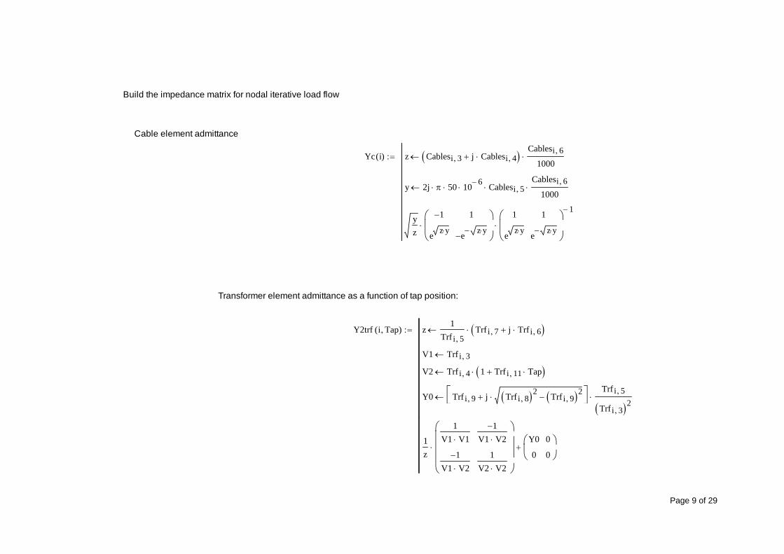
Build the impedance matrix for nodal iterative load flow

Cable element admittance

Yc i( ) z Cablesi 3 j Cablesi 4 Cablesi 6

1000

y 2j 50 10 6 Cablesi 5

Cablesi 61000

yz

1

e z y

1

e z y

1

e z y

1

e z y

1

Transformer element admittance as a function of tap position:

Y2trf i Tap( ) z1

Trf i 5Trfi 7 j Trf i 6

V1 Trfi 3

V2 Trfi 4 1 Trf i 11 Tap

Y0 Trfi 9 j Trf i 8 2 Trf i 9 2

Trfi 5

Trfi 3 2

1z

1V1 V1

1V1 V2

1V1 V2

1V2 V2

Y0

0

0

0

Page 9 of 29

Shunts

Yshunt i( )Shunti 4 j Shunti 3

Shunti 2 2

Nodal admittance matrixas a function of transformertap positions

N rows Vn( )

rE 10 12 Zbus Tap( ) YN N 0

Y1 11rE

Yx Yc i( )

YCablesi r Cablesi c YCablesi r Cablesi c Yxr c

c 1 2for

r 1 2for

i 1 rows Cables( )for

Yx Y2trf i Tapi

YTrf i r Trf i c YTrf i r Trf i c Yxr c

c 1 2for

r 1 2for

i 1 rows Trf( )for

YShunti 1 Shunti 1 YShunti 1 Shunti 1 Yshunt i( )

i 1 rows Shunt( )for

Y 1

rE = Thevenin resistance of 400 kV Interface Point voltagesource at node 1

Page 10 of 29

Element power flow formulae for later use

Power in cable i at end =1,2 as a function of nodal voltages. Positive = from end 1 to end 2 Sc i end V( ) z Cablesi 3 j Cablesi 4

Cablesi 61000

y 2j 50 10 6 Cablesi 5

Cablesi 61000

K1

e z y

1

e z y

1 V Cablesi 1 V Cablesi 2

V Cablesi 1 V Cablesi 2

end

yz

K1 e z y end 1( ) K2 e z y end 1( )

Power in transformer i at end =1,2 as a function of nodal voltages. Positive = from end 1 to end 2 St i end Tap V( ) z

Trf i 3 2

Trf i 5Trfi 7 j Trf i 6

nTrf i 3

Trfi 4 1 Trf i 11 Tap

Y0 Trfi 9 j Trf i 8 2 Trf i 9 2

Trfi 5

Trfi 3 2

V Trf i 1 V Trf i 2 n

zY0 V Trf i 1

V Trf i 1

end 1=if

V Trf i 1 V Trf i 2 n

z

n V Trf i 2 otherwise

Page 11 of 29

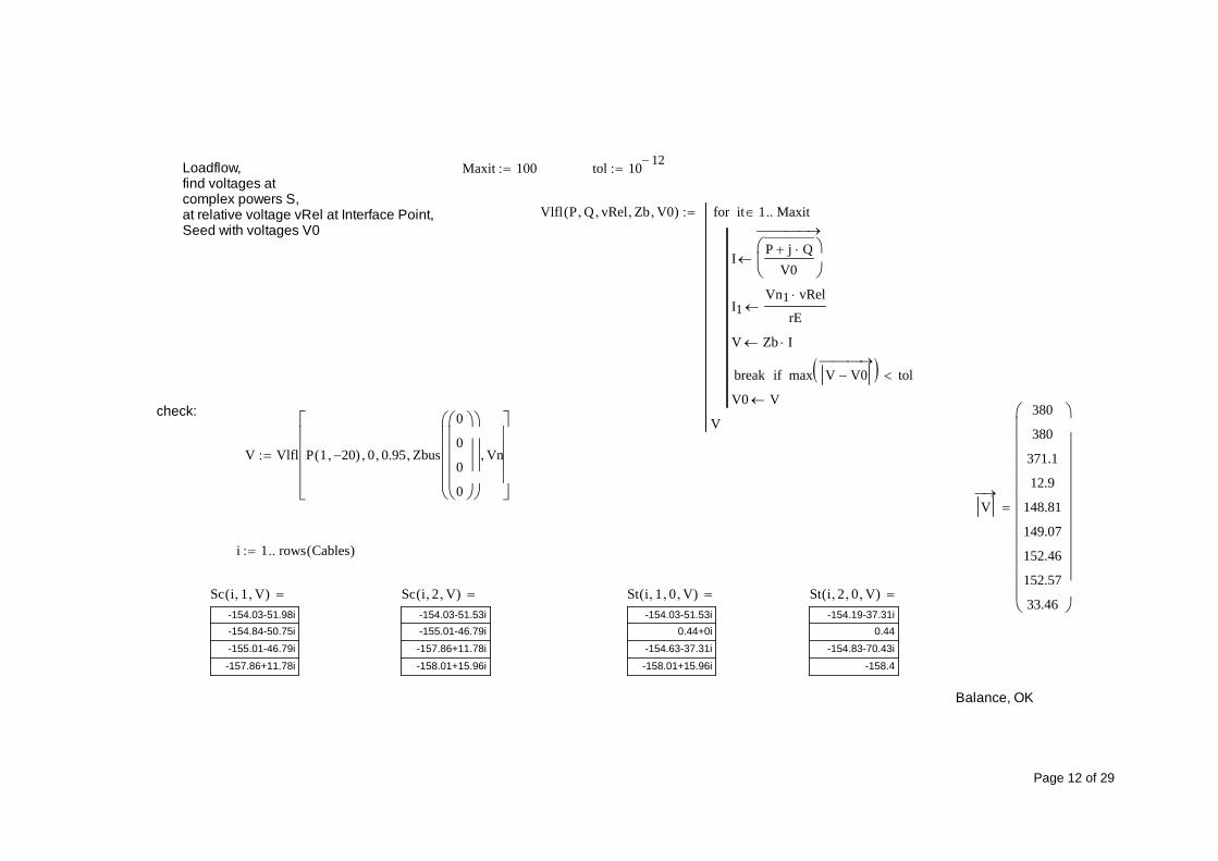
Loadflow,find voltages atcomplex powers S,at relative voltage vRel at Interface Point,Seed with voltages V0

Maxit 100 tol 10 12

Vlfl P Q vRel Zb V0( )

IP j Q

V0

I1Vn1 vRel

rE

V Zb I

break max V V0 tolif

V0 V

it 1 Maxitfor

V

check:

V Vlfl P 1 20( ) 0 0.95 Zbus

0

0

0

0

Vn

V

380

380

371.1

12.9

148.81

149.07

152.46

152.57

33.46

i 1 rows Cables( )

Sc i 1 V( )-154.03-51.98i-154.84-50.75i

-155.01-46.79i

-157.86+11.78i

Sc i 2 V( )-154.03-51.53i-155.01-46.79i

-157.86+11.78i

-158.01+15.96i

St i 1 0 V( )-154.03-51.53i

0.44+0i

-154.63-37.31i

-158.01+15.96i

St i 2 0 V( )-154.19-37.31i

0.44

-154.83-70.43i

-158.4

Balance, OK

Page 12 of 29

Model the reactive power controllers:

ParkPilot, controls 150 kV onshore reactive power by a voltage control slope arrangement

Mvar baseTarget voltage, relativeSlope (note: 8.68% = equivalent to 5% base 30 Mvar)Controlled cable no.-at end 1 or 2Controlled turbine eqivalent at node

ParkPilot

PmaxPPM tan acos 0.95( )( )

107%

8.68%

2

1

9

Target:QPPtarget V( )

ParkPilot2

V Cables ParkPilot4 ParkPilot5

Vn Cables ParkPilot4 ParkPilot5

ParkPilot3ParkPilot1

Actual measurement at voltages V QPP V( ) Im Sc ParkPilot4 ParkPilot5 V

Page 13 of 29

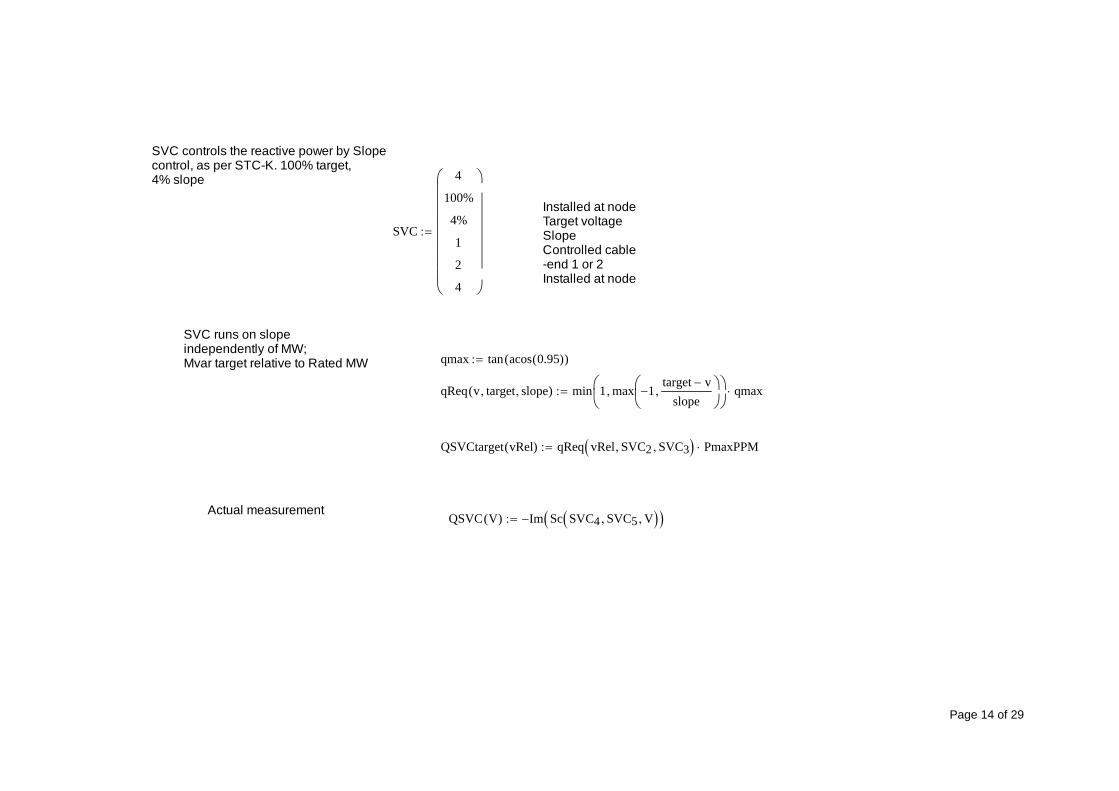
SVC controls the reactive power by Slopecontrol, as per STC-K. 100% target,4% slope

Installed at nodeTarget voltageSlopeControlled cable-end 1 or 2Installed at node

SVC

4

100%

4%

1

2

4

SVC runs on slopeindependently of MW; Mvar target relative to Rated MW qmax tan acos 0.95( )( )

qReq v target slope( ) min 1 max 1target v

slope

qmax

QSVCtarget vRel( ) qReq vRel SVC2 SVC3 PmaxPPM

Actual measurementQSVC V( ) Im Sc SVC4 SVC5 V

Page 14 of 29

Iterate reactive powersto target relative turbine voltageCap turbine reactive power to SWT limits

nSVC SVC6 nTurbine ParkPilot6 acc 1

dQdQ 0.5

VQ pRel vRel Tap V Q( ) QnewN 0

Zb Zbus Tap( )

V V acc Vlfl P pRel QnSVC Q vRel Zb V V

QnewnTurbine QnTurbine dQdQ QPPtarget V( ) QPP V( )( )

QnewnSVC QnSVC dQdQ QSVCtarget vRel( ) QSVC V( )( )

ri QnewnTurbine j QnewnSVC

break max Qnew Q 0.001if

Q Q acc Qnew Q( )

i 1 Maxitfor

V

Q

i

r

Page 15 of 29

OK

St i 2 0 V( )-154.28+37.5i

0.62+39.6i

-155.06-30.72i

-158.4+50.48i

St i 1 0 V( )-154.14+26.03i

0.62+42.98i

-154.9-5.47i

-157.99+67.46i

Sc i 2 V( )-154.14+26.03i

-155.21-3.81i

-157.82+62.85i

-157.99+67.46i

Sc i 1 V( )-154.13+25.51i

-155.07-8.42i

-155.21-3.81i

-157.82+62.85i

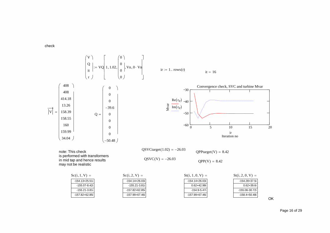
QPP V( ) 8.42QSVC V( ) 26.03

QPPtarget V( ) 8.42note: This checkis performed with transformersin mid tap and hence results may not be realistic

QSVCtarget 1.02( ) 26.03

Q

0

0

0

39.6

0

0

0

0

50.48

V

408

408

414.18

13.26

158.39

158.55

160

159.99

34.04

0 5 10 15 2060

50

40

30Convergence check, SVC and turbine Mvar

Iteration no

Mva

r

Re rir Im rir

ir

it 16ir 1 rows r( )

V

Q

it

r

VQ 1 1.02

0

0

0

0

Vn 0 Vn

check

Page 16 of 29

Eliminate the unknownt transformer tapings -tap transformers into position; calculate losses for steady state

changeTap V tap( )

v V Trf i 2

vn Trf i 10 Trfi 4

tapi tapi sign vn v( ) v vnTrfi 12

2Trf i 4if Trf i 11 0if

i 1 rows Trf( )for

tap

VQtap pRel vRel Tap V Q( )

vq VQ pRel vRel Tap V Q( )

Tap1 changeTap vq1 Tap

break Tap1 Tap=if

Tap Tap1

V vq1

Q vq2

i 1 Maxitfor

vq5 Tap

vq

i Maxitif

0 otherwise

Page 17 of 29

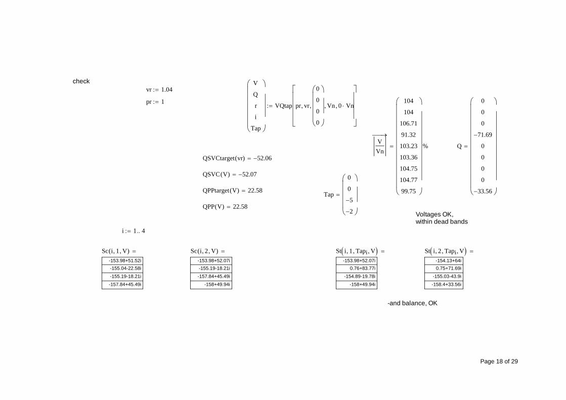
-and balance, OK

St i 2 Tapi V -154.13+64i0.75+71.69i

-155.03-43.9i

-158.4+33.56i

St i 1 Tapi V -153.98+52.07i

0.76+83.77i

-154.89-19.78i

-158+49.94i

Sc i 2 V( )-153.98+52.07i-155.19-18.21i

-157.84+45.49i

-158+49.94i

Sc i 1 V( )-153.98+51.52i-155.04-22.58i

-155.19-18.21i

-157.84+45.49i

i 1 4

Voltages OK,within dead bands

QPP V( ) 22.58

Tap

0

0

5

2

QPPtarget V( ) 22.58

QSVC V( ) 52.07

QSVCtarget vr( ) 52.06

Q

0

0

0

71.69

0

0

0

0

33.56

V

Vn

104

104

106.71

91.32

103.23

103.36

104.75

104.77

99.75

%

V

Q

r

i

Tap

VQtap pr vr

0

0

0

0

Vn 0 Vn

pr 1

vr 1.04check

Page 18 of 29

Which elements of the wind farm are the predominanly lossy ones?

150 kV

33 kV

SGT1A

GT1

HPPP1

SVC

MSR

Grid Entry Point

EXPO

RT C

ABLE

1

harmonicfilter

NGET1

2

3 (fictitious, y-equivalent)

4

5

6

7

8

9

to SGT1B

Single systemto which the

formula applies

MWh MWh

Blue: Node numbersapplied in the calculations

LossContributions pRel( ) V VQtap pRel 101%

0

0

0

0

Vn 0 Vn

Tap V5

V V1

dPGT St 4 1 Tap4 V St 4 2 Tap4 V

dPExp Sc 2 1 V( ) Sc 4 2 V( )

dPFilter St 3 2 Tap3 V Sc 2 1 V( )

dPSVC St 2 2 Tap2 V PonshoreAux

dPSGT St 1 1 Tap1 V St 2 2 Tap2 V St 3 2 Tap3 V

dP400 Sc 1 1 V( ) Sc 1 2 V( )

dPAll Sc 1 1 V( ) St 4 2 Tap4 V

Re dPGT dPExp dPFilter dPSVC PonshoreAux dPSGT dP400( )T Re dPAll( )

Calculatedfor the NGETaverage voltageof 101% x 400 kV

Offshore transformer150 kV export cable150 kV filterSVCOnshore substation aux supplyOnshore transformer400 kV connections

LossContributions 0( )

16.3

13.2

1.3

33.1

24.9

11.2

0

% LossContributions AveragePower( )

12.7

46.7

0.7

17.1

13.5

9.2

0

% LossContributions 1( )

9.4

69

0.2

9.9

4.3

7.2

0

%

Page 19 of 29

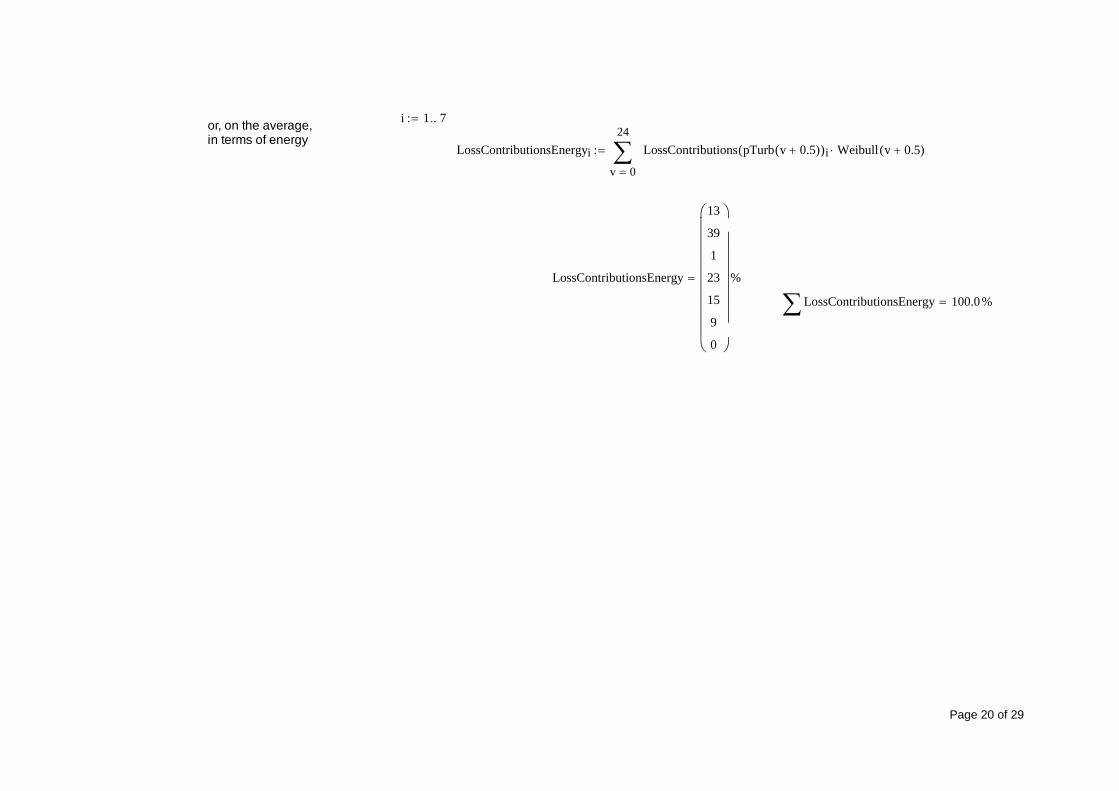
i 1 7or, on the average,in terms of energy

LossContributionsEnergyi0

24

v

LossContributions pTurb v 0.5( )( )i Weibull v 0.5( )

LossContributionsEnergy

13

39

1

23

15

9

0

%

LossContributionsEnergy 100.0%

Page 20 of 29

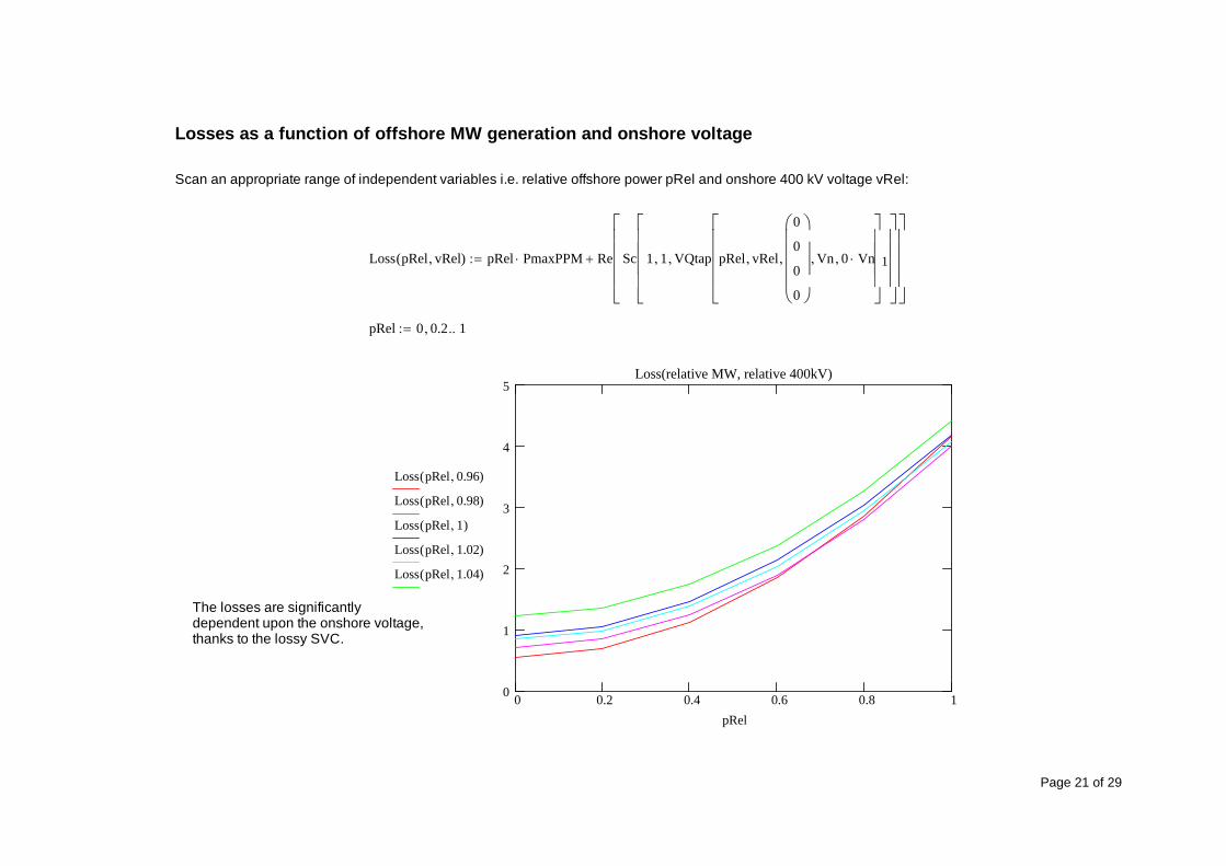
Losses as a function of offshore MW generation and onshore voltage

Scan an appropriate range of independent variables i.e. relative offshore power pRel and onshore 400 kV voltage vRel:

Loss pRel vRel( ) pRel PmaxPPM Re Sc 1 1 VQtap pRel vRel

0

0

0

0

Vn 0 Vn

1

pRel 0 0.2 1

0 0.2 0.4 0.6 0.8 10

1

2

3

4

5Loss(relative MW, relative 400kV)

Loss pRel 0.96( )

Loss pRel 0.98( )

Loss pRel 1( )

Loss pRel 1.02( )

Loss pRel 1.04( )

pRel

The losses are significantlydependent upon the onshore voltage,thanks to the lossy SVC.

Page 21 of 29

Elimination of voltage as an unknown

A loss correction formula can only have the active power P as an argument. The voltage is thus to be eliminated.

Two approaches will be used: A) a statistical assumption and B) historical voltage recordings from the substations adjacent to the Cleve Hill connection point.

A) Below, Grid Code CC.6.1.5 is applied, assuming the nominal 400 kV to be the mean and the +/-5% range to be the symmetrical 99% percentile limits of a normally distributed voltage

Percentile 95% Bins 5 v 0.9 0.91 1.1

f v( ) dnorm v 15%

qnorm 11 Percentile

2 0 1

0.8 0.9 1 1.10

10

20

f v( )

v

i 1 Bins

pi f 1105% 95%

Binsi

Bins 12

P p

ppP

p 1 p

0.1

0.24

0.33

0.24

0.1

loss pRel( )

1

Bins

i

pi Loss pRel 110%Bins

iBins 1

2

Note: 5, 7 or 11 Bins give virtually the same loss result

Page 22 of 29

Averaged loss shown in redon top of previous figure:

0 0.2 0.4 0.6 0.8 10

1

2

3

4

5Loss(relative MW, relative 400kV)

Loss pRel 0.96( )

Loss pRel 0.98( )

Loss pRel 1( )

Loss pRel 1.02( )

Loss pRel 1.04( )

loss pRel( )

pRel

Percentile 0.95

loss pRel( )0.8470.9911.4212.1253.0984.333

Percentile 0.95

loss pRel( )0.850.981.392.052.974.13

check: also computed for voltage Percentiles 95%rather than above 99%, nosignificant difference

Page 23 of 29

B) Now try with recorded voltages at Kemsley and Canterbury, all VTs of all circuits, for one year August 2010- July 2011 (8). The large amount of data has been cleaned for invalid data and apportioned in bins in separate Mathcad spreadsheet

Middle of bin, kV / probability of bin

VoltageDistribution

390.625

397.625

399.969

401.769

403.3

404.812

406.406

408.194

410.381

414.531

0.103

0.085

0.111

0.095

0.087

0.118

0.097

0.109

0.09

0.102

lossHistV pRel( )

1

rows VoltageDistribution( )

i

VoltageDistributioni 2 Loss pRelVoltageDistributioni 1

400

lossHistV pRel( )0.86

11.422.07

34.18

loss pRel( )0.850.981.392.052.974.13

NGET's voltage recordings yield slightly higher losses than the normal assumptions. Hence, the formula derived from the recordings will be used.

loss pRel( ) lossHistV pRel( )

Page 24 of 29

The maximum inaccuracy of the polynomial approximation is 1%.

A0 0.87

A2 3.35

Compare the exact formula and the polynomial approximation:

0 0.2 0.4 0.6 0.8 10.02

0.01

0

0.01

A0 A2 pRel2 dPdP

pRel

A0

A2

Minimize Err A0 A2( )

Givenoptimisation

A2 2Err A0 A2( )

1

Steps

i

dPi x A0 A2 i( ) 2

A0 dP1variable seeds

x A0 A2 i( ) A0 A2 pReli 2Find the 2nd order coefficient

by minimisation of error

Use the common approach ofno-load + load losses, zero-2nd orderpolynomium

dP1 0.86

dPi loss pReli

pRelii 1Steps

i 1 Steps 1Compute vectors of

independent and dependentvariables for fitting

Steps 10Approximate by a ploynomium

Page 25 of 29

That is: A good approximation for the MW losses as a function of pRel i.e. offhore active power base an installed nominal turbine capacity of 44 off 3.6 MWturbines is

P pRel( ) A0 A2 pRel2

This formula needs conversion to offshore and onshore power in MWh/0.5 h C 0.5 1 MW = 0.5 MWh/½ h

M0 C A0 M2 C A2

1C

2

PmaxPPM2

M0

M2

0.4334

2.6705 10 4

I.e:

Ponshore Poffshore( ) Poffshore 0.4334 2.6705 10 4 Poffshore2

[MWh per ½ h], MWh per ½ h]

Relate the losses to the annual generation into the Grid Entry Points

Relative energy losses:

dw0

25vP pTurb v( )( ) Weibull v( )

d

44 3.6 AveragePower

dw 2.79%

Page 26 of 29

Guesswork 2.44%Guesswork 1.82 %( )2 1.45 %( )2

0.72 %( )2 0.13%( )2

Overall uncertainty incurring from guesswork:

PonshoreAux 50 %AveragePower 44 3.6( )

0.13%Substation loads are probably not at LV installation dimentioning limits at all times:

insignificantdw1% dw0%dw0%

0.72%dw1% 2.81%

dw0% 2.79%

Look at robustness to export cable lengthsAt the time of calculating this, cables have not yet been laid; applied budget dx = 0% has worst-case assumptions in it so as to buy enough cable

insignificantdwB

dwA951 1.45%

dwB 2.79%

dwA95 2.75%

dwA99 2.75%

Look at the 400 kV voltage distribution assumptionRedone for CC.6.1.4 voltage limits being 95% percentiles rather than 99% percentiles:

1.82% 2.79 % 0.05%That is: Cable temperature assumption is of minor influence,0.15% of annual energy delivered to the grid

dw40 dw202 dw29_75

1.82%dw40 2.79%

dw20 2.69%

dw29_75 2.74%

Look at the initial cable core temperature assumptionRedone for 20 and 80 deg average cable temperature, spreadsheet rerun manually changing above AverageCableTemperature 40

Assess the effect of assumptions made

Page 27 of 29

Accuracy budget

For a normal COP 1 metering installation with class 0.2 elements, the overall uncertainty budget looks as follows:

VT 0.2%

CT 0.2%

Meter 0.2%

COP1 VT2

CT2

Meter2

COP1 0.35%

When translating to onshore connection by a loss formula, the accuracy of that formula needs to be taken into account.Further to assumptions uncertainty, allow also for 10% on cable resistances, substation losses and SVC losses. The overall uncertainty on the formula, including the polynomial approximation, is not more than:

General 10%

Formula 2.44%( )2General

2 Formula 10.29%

Hence:

Overall COP12

dw Formula 2

Overall 0.45% OverallCOP1

1.3

COP 1 accuracy is hence violated at the onshore interface point.

Page 28 of 29

However, COP 2 accuracy is maintained:

COP2 3 0.5 %OverallCOP2

0.52

Coarse capital value of inaccuracy for 1st yearduring which only 22 out of 44 turbines are inoperation on the average, at £ 160 per MWh:

Overall2

COP12

8760 22 3.60

25vpTurb v( ) Weibull v( )

d

160 137345

This is the extreme when full uncertainty applies, not to be expected.

A meter installation cannot be justified.

Page 29 of 29