shuyu sun earth science and engineering program kaust presented at the 2009 annual utam meeting,...
TRANSCRIPT

Shuyu SunEarth Science and Engineering program
KAUST
Presented at the 2009 annual UTAM meeting, 2:05-2:40pm January 7, 2010 at the Sutton Building, University of Utah, Salt Lake City, Utah

Energy and Environment Problems


Single Phase Flow in Porous Media
• Continuity equation – from mass conservation
• Thermodynamic model
• For impressible fluid (constant density):
• Still need one more equation
€
∂ρ∂t
+∇ ⋅ ρu( ) = qm , (x, t)∈ Ω × (0,T]
€
ρ =ρ(T,P)
€
∇⋅u = q (x, t)∈ Ω × (0,T]

Relate velocity with pressure: Darcy's law
• Experiment by Henry Darcy (1855–1856)

Darcy's law
• Can be derived from the Navier-Stokes equations via homogenization.
• It is analogous to – Fourier's law in the field of heat conduction,– Ohm's law in the field of electrical networks,– Fick's law in diffusion theory.
• In 3D:

Incompressible Single Phase Flow
• Continuity equation
• Darcy’s law
• Boundary conditions:
],0(),( Ttxq u
],0(),( Ttxp K
u
€
p = pB (x, t)∈ ΓD × (0,T]
u ⋅n = uB (x, t)∈ ΓN × (0,T]

Transport in Porous Media
• Transport equation
• Boundary conditions
• Initial condition
• Dispersion/diffusion tensor
],0(),()()( * Ttxcrqccct
c
uDu
€
uc − D∇c( ) ⋅n = cBu ⋅n t ∈ (0,T], x ∈ Γin (t)
−D∇c( ) ⋅n = 0 t ∈ (0,T], x ∈ Γout (t)
xxcxc )()0,( 0
)()()( uEIuEuIuD tlmD
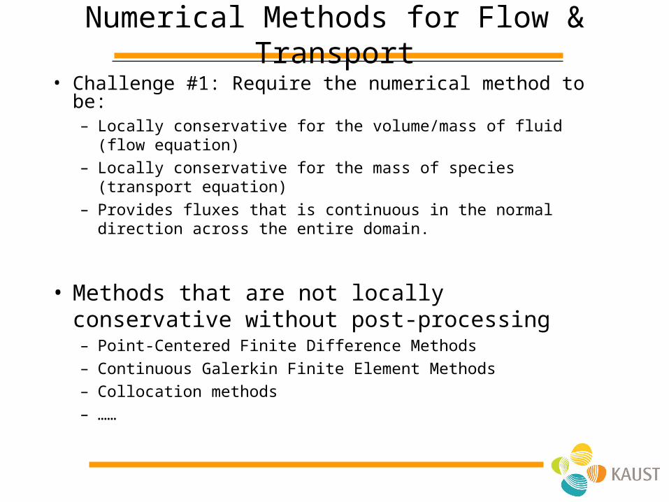
Numerical Methods for Flow & Transport
• Challenge #1: Require the numerical method to be: – Locally conservative for the volume/mass of fluid (flow
equation) – Locally conservative for the mass of species (transport
equation) – Provides fluxes that is continuous in the normal direction
across the entire domain.
• Methods that are not locally conservative without post-processing– Point-Centered Finite Difference Methods– Continuous Galerkin Finite Element Methods – Collocation methods– ……

Example: importance of local conservation

Example: importance of local conservation

Numerical Methods for Flow & Transport
• Challenge #2: Fractured Porous Media – Different spatial scale: fracture much smaller– Different temporal scale: flow in fracture much faster
• Solutions:– Mesh adaptation for spatial scale difference– Time step adaptation for temporal scale difference

Example: flow/transport in fractured media

Example: flow/transport in fractured media
Locally refined mesh:
FEM and FVM are better than FDfor adaptive meshes and complex geometry

Example: flow/transport in fractured media
CFL condition requires much smaller time step in fractures than in matrix: adaptive time stepping.

Numerical Methods for Flow & Transport
• Challenge #3: Sharp fronts or shocks – Require a numerical method with little numerical diffusion – Especially important for nonlinearly coupled system, with
sharp gradients or shocks easily being formed
• Solutions:– Characteristic finite element methods – Discontinuous Galerkin methods

Example: Comparison of DG and FVM
Advection of an injected species from the left boundary under constant Darcy velocity. Plots show concentration profile at 0.5 PVI.
Upwind-FVM on 40 elements Linear DG on 40 elements

Example: Comparison of DG and FVM
Flow in a medium with high permeability region (red) and low permeability region (blue) with flow rate specified on left boundary. Contaminated fluid flood into clean media.

Example: Comparison of DG and FVM
Advection of an injected species from the left. Plots show concentration profiles at 3 years (0.6 PVI).
FVM Linear DG

Numerical Method for Flow & Transport
• Challenge #4: Time dependent local phenomena– For example: moving contaminant plume
• Solutions:– Dynamic mesh adaptation
• Based on conforming mesh adaptation• Based on non-conforming mesh adaptation

Adaptive DG methods – an example
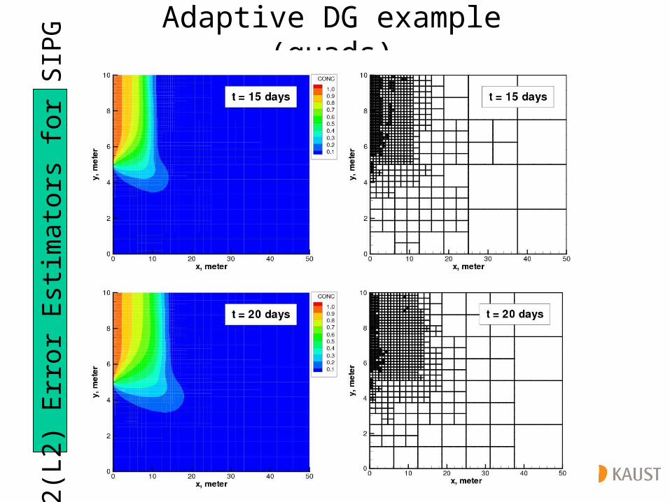
• Sorption occurs only in the lower half sub-domain,
• SIPG is used.

Adaptive DG example (cont.)
Ani
sotr
opic
mes
h ad
apta
tion

Adaptive DG example (cont.)
Est
imat
ors
usin
g hi
erar
chic
bas
es
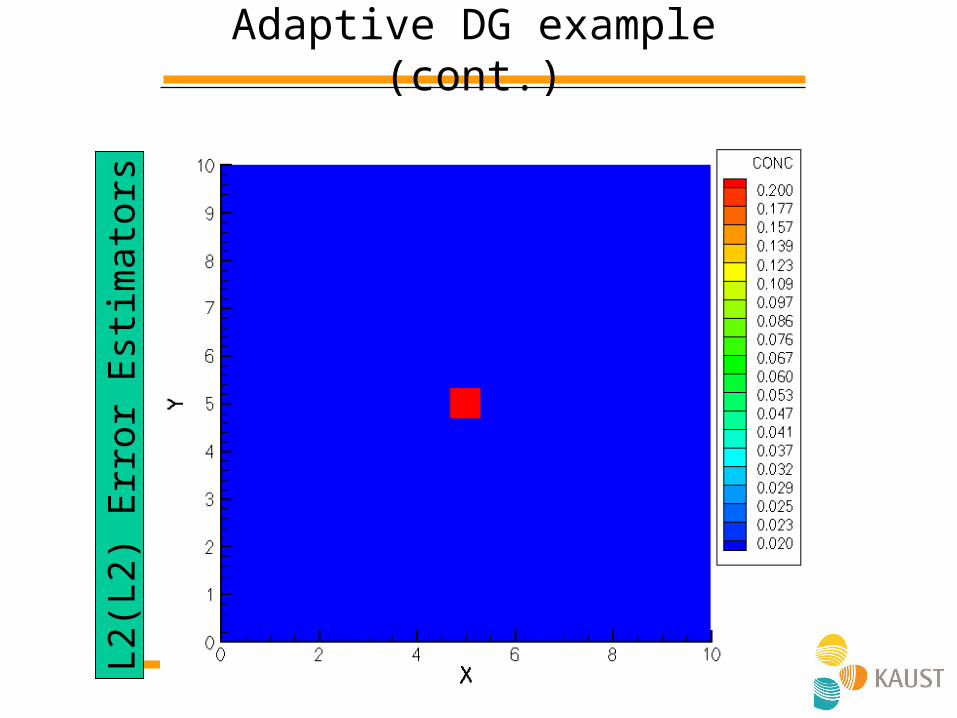
Adaptive DG example (cont.)
L2(
L2)
Err
or E
stim
ator
s

A Posteriori Error Estimators
• Residual based – L2(L2)– L2(H1)
• Implicit – Solve a dual problem, can give estimates on a target
functional– Disadvantages: computational costly and not flexible– Advantages: More accurate estimates
• Hierarchical bases – Brute-force: difference between solutions of two
discretizations (most expensive)– Local problems-based – Advantage: can guide anisotropic hp-adaptivity
• Superconvergence points-based – Difficult for unstructured and non-conforming meshes

A posteriori error estimates
• Residuals– Interior residuals
– (Element-)boundary residuals
DGDGDG
DGDGI CC
t
CCMrqCR
Du)(*
outhDG
inhDGDG
B
hDG
B
DirihBDG
hDG
B
xC
xCCc
xC
R
xcC
xCR
,
,1
,
0
nD
nDuu
nD
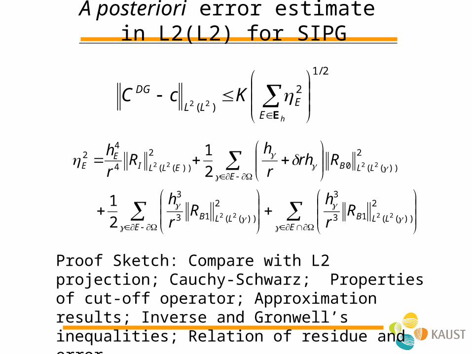
A posteriori error estimate in L2(L2) for SIPG
2/1
2
)( 22
hEELL
DG KcCΕ
ELLB
ELLB
ELLBELLI
EE
Rr
hR
r
h
Rrhr
hR
r
h
2
))((13
32
))((13
3
2
))((0
2
))((4
42
2222
2222
2
1
2
1
Proof Sketch: Compare with L2 projection; Cauchy-Schwarz; Properties of cut-off operator; Approximation results; Inverse and Gronwell’s inequalities; Relation of residue and error

Dynamic mesh adaptation with DG
• Nonconforming meshes– Effective implementation of mesh
adaptation,– Elements will not degenerate unless using
anisotropic refinement on purpose.
• Dynamic mesh adaptation – Time slices = a number of time steps; only
change mesh for time slices. – Refinement + coarsening number of
elements remain constant.
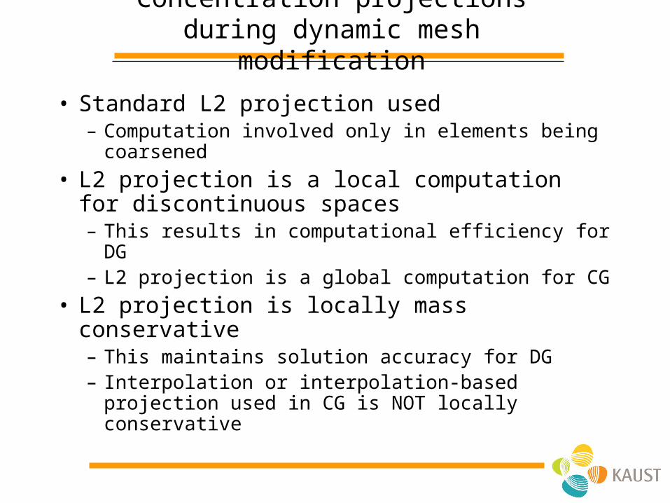
Concentration projections during dynamic mesh modification
• Standard L2 projection used– Computation involved only in elements being
coarsened
• L2 projection is a local computation for discontinuous spaces– This results in computational efficiency for DG– L2 projection is a global computation for CG
• L2 projection is locally mass conservative– This maintains solution accuracy for DG– Interpolation or interpolation-based projection
used in CG is NOT locally conservative

Adaptive DG example (quads)L
2(L
2) E
rror
Est
imat
ors
for
SIP
G
Adaptive DG example (quads)L
2(L
2) E
rror
Est
imat
ors
for
SIP
G

Adaptive DG example (quads)L
2(L
2) E
rror
Est
imat
ors
for
SIP
G

Adaptive DG (with triangles)
L2(
L2)
Err
or E
stim
ator
s on
Tri
angl
es
Initial mesh

Adaptive DG (with triangles)
L2(
L2)
Err
or E
stim
ator
s on
Tri
angl
es
T=0.5
T=1.0

Adaptive DG (with triangles)
L2(
L2)
Err
or E
stim
ator
s on
Tri
angl
es
T=1.5
T=2.0

Adaptive DG example in 3DL
2(L
2) E
rror
Est
imat
ors
on 3
D
T=1.5
T=2.0
T=0.1 T=0.5 T=1.0

ANDRA-Couplex1 case
Background– ANDRA: the French National Radioactive Waste Management Agency
– Couplex1 Test Case• Nuclear waste management: Simplified 2D Far Field model• Flow, Advection, Diffusion-dispersion, Adsorption
Challenges– Parameters are highly varying
• permeability; retardation factor; effective porosity; effective diffusivity
– Very concentrated nature of source• concentrated in space • concentrated in time
– Long time simulation• 10 million years
– Multiple space scales• Around source / Far from source
– Multiple time scales• Short time behavior (Diffusion dominated) • Long time behavior (Advection dominated)

ANDRA-Couplex1 case (cont.)
200k years
2m years


Compositional Three-Phase Flow
• Mass Conservation (without molecular diffusion)
• Darcy’s Law
gowPkr ,,, ρ
gKu
gow
ii xc,,
,
uU
Numerical Modeling for Flow & Transport
• Challenge #5: Importance of capillarity – Capillary pressure usually ignored in compositional flow
modeling– Even the immiscible two-phase flow or the black oil model
usually assumes only a single capillary function (i.e. assuming a single uniform rock)

• Two-dimensional 400x200m^2 domain • Contains a less-permeable (K=1md) rock in the center
of the domain while the rest has K=100md. Isotropic permeability tensor used.
• Porosity = 0.2 • Densities: 1000 kg/m^3 (W) and 660 kg/m^3 (O)• Viscosities: 1 cp (W) and 0.45 cp (O) • Inject on the left edge, and produce on the right edge• Injection rate: 0.1 PV/year• Initial water saturation: 0.0; Injected saturation: 1.0
Example: Reservoir Description

• Relative permeabilities (assuming zero residual saturations):
• Capillary pressure
Reservoir Description (cont.)
2,,1, mSSSkSk wwem
wernmwerw
bars50 and5,,log)( cwwewecwec BSSSBSp
K=100md
K=1md

Discretization • DG-MFE-Iterative • Pressure time step: 10years / 1000 timeSteps• Saturation time step = 1/100 pressure time step• Mesh: 32x64 uniform rectangular grid:

Comparison: if ignore capillary pressure …
Saturation at 10 years: Iter-DG-MFE
With nonzero capPres
With zero capPres

Numerical Modeling for Flow & Transport
• Challenge #6: Discontinuous saturation distribution– Saturation usually is discontinuous across different rock
type, which is ignored in many works in literature – When permeability changes, the capillary function usually
also changes!
• Solutions: – Discontinuous Galerkin methods
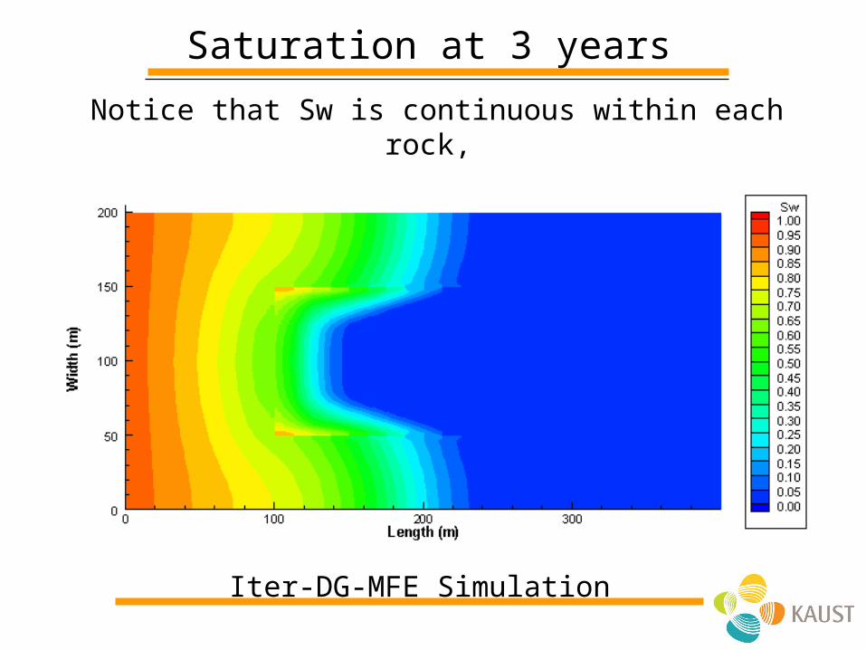
Saturation at 3 years
Iter-DG-MFE Simulation
Notice that Sw is continuous within each rock, but Sw is discontinuous across the two rocks
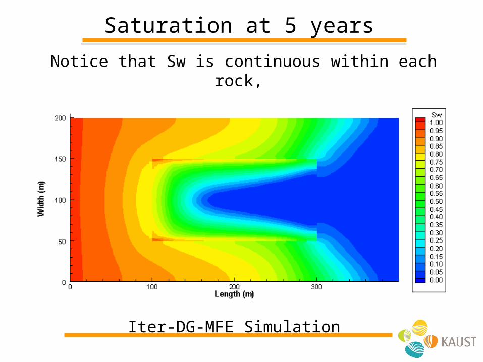
Saturation at 5 years
Iter-DG-MFE Simulation
Notice that Sw is continuous within each rock, but Sw is discontinuous across the two rocks

Saturation at 10 years
Iter-DG-MFE Simulation
Notice that Sw is continuous within each rock, but Sw is discontinuous across the two rocks

Water pressure at 10 years
Iter-DG-MFE Simulation (pressure unit: Pa)
Notice that Pw is continuous within the entire domain.

Capillary pressure at 10 years
Iter-DG-MFE Simulation (pressure unit: Pa)
Notice that Pc is continuous within the entire domain.

Numerical Modeling for Flow & Transport
• Challenge #7: Multiscale heterogeneous permeability
– Fine scale permeability has pronounced influence on coarse scale flow behaviors
– Direct simulation on fine scale is intractable with available computational power
• Solutions: – Upscaling schemes – Multiscale finite element methods

Recall: DG scheme for flow equation
• Bilinear form
• Linear functional
• Scheme: seek such that
hDD
hhh
Eee
e
e
ee e
ee e
Eee e
Eee e
TEE
wph
pK
spK
pK
spK
pK
pa
]][[
]}[{]}[{),(
form
form
nn
nn
ND e
e Be
e Be upK
sql
nform),()(
)( hkh TDp
)()(),( hkh TDvvlvpa
IIPG SIPG,0
NIPG0
DG-OBB0
IIPG0
NIPG DG,-OBB1
SIPG1
form
s
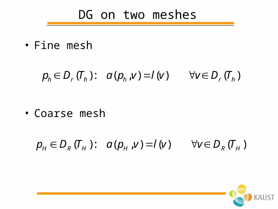
DG on two meshes
• Fine mesh
• Coarse mesh
( ): ( , ) ( ) ( )h r h h r hp D T a p v l v v D T
( ): ( , ) ( ) ( )H R H H R Hp D T a p v l v v D T

Space decomposition
• Introduce
• Solution
( ) ( )r h R H fD T D T V
( ), :
( , ) ( ) ( , ) ( )
( , ) ( ) ( , )
H R H f f
H f R H
f H f
p D T p V
a p v l v a p v v D T
a p v l v a p v v V
fV
.h H fp p p

Closure Assumption
• Introduce
• Two-scale solution
0 : 0,f f HEV v V v E T
0 0
0
0 0
( ), :
( , ) ( ) ( , ) ( )
( , ) ( ) ( , )
H R H f f
H f R H
f H f
p D T p V
a p v l v a p v v D T
a p v l v a p v v V
0fV
0.MS H fp p p

Implementation
• Multiscale basis functions:For each
• Multiscale approximation space:
• Two-scale DG solution
0( ) : ( )MS f H H R HV v v v D T
: ( , ) ( ) ,MS MS MS MSp V a p v l v v V
0 0
0 0
( ) :
( ( ), ) ( ) ( , )
f H f
f H H f
v v V
a v v v l v a v v v V
( )H R Hv D T

Other Closure Options
• Local problems for solving multiscale basis functions need a closure assumption.
• In previous derivation, we strongly impose zero Dirichlet boundary condition on local problems.
• Other options: – Weakly impose zero Dirichlet boundary condition on local
problems. – Strongly impose zero Neumann boundary condition on local
problems.– Weakly impose zero Neumann boundary condition on local
problems.– Combination of zero Neumann and zero Dirichlet.
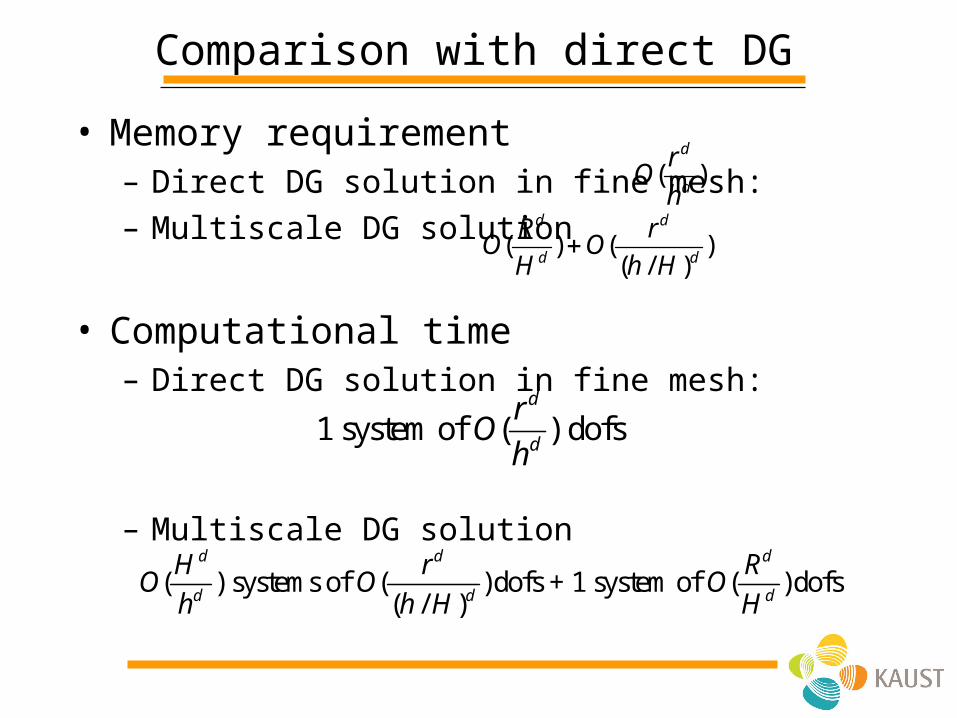
Comparison with direct DG
• Memory requirement– Direct DG solution in fine mesh: – Multiscale DG solution
• Computational time – Direct DG solution in fine mesh:
– Multiscale DG solution
( )d
d
rO
h
( ) ( )( / )
d d
d d
R rO O
H h H
1 system of ( ) dofsd
d
rO
h
( ) systems of ( )dofs + 1 system of ( )dofs( / )
d d d
d d d
H r RO O O
h h H H

Example
• Conductivity:
• Boundary conditions: – Left: p=1; Right: p=0; top & bottom: u=0.
• Discretization: – R=r=1; – Coarse mesh 16x16; Fine mesh 256x256

Example (cont.)
Coarse DG solution Brute-force Fine DG solution

Example (cont.)
Multiscale DG solution Brute-force Fine DG solution

Future work
• Multiscale DG methods for compositional multiple-phase flow in heterogeneous media,
• Stochastic PDE simulations,• Multigrid solver for DG (including p-multigrid), • Other future works:
– Automatically adaptive time stepping,– Implicit a posteriori error estimators, – Fully automatically hp-adaptivity for DG, – A posteriori estimators for coupled reactive transport
and flow.