sic: a 1d hydrodynamic m r irrigation canal · pdf filesic: a 1d hydrodynamic model for river...
TRANSCRIPT

CAPÍTULO 1
SIC: A 1D HYDRODYNAMIC MODEL FOR RIVER AND IRRIGATION CANAL MODELING AND REGULATION
por
Jean-Pierre Baume & Pierre-Olivier Malaterre1 Gilles Belaud2
Benoit Le Guennec3
1 UMR G-EAU, Cemagre - 361 rue Jean-François Breton - BP 5095, 34196 Montpellier cedex 5, France - [email protected] ; [email protected] ; http://www.cemagref.net2 UMR G-EAU, Agro Montpellier - , place Pierre Viala - 34060 Montpellier cedex, France - [email protected] IRD - HYBAM - UR 154 LMTG - Programa de Engenharia Oceânica COPPE/UFRJ - Área de Engenharia Costeira e Oceanográafica - Caixa Postal 68 508, 21945-970 Rio de Janeiro, RJ - [email protected] ; http://www.oceanica.ufrj.br

2 Baume & Malaterre; Belaud; Le Guennec
Conteúdo
1.1. General ....................................................................................5 1.1.1. Main features ...................................................................5 1.1.2. Software dedicated to irrigation canals .............................7 1.1.3. Advanced user-friendly interfaces .....................................8
1.2. Theoretical aspects ...................................................................9 1.2.1. Topology and geometry....................................................9 1.2.2. Topology..........................................................................9 1.2.3. Geometry ........................................................................9 1.2.4. Mathematical formulation of the problem ......................10 1.2.5. The de Saint-Venant equations.......................................10 1.2.6. Equation of the reach backwater curve...........................11 1.2.7. Head loss evaluation ......................................................12
1.2.7.1. Friction loss evaluation.............................................12 1.2.7.2. Momentum coefficient evaluation............................12
1.2.8. Cross structures ..............................................................13 1.2.8.1. Weir / Orifice (high sill elevation) .............................13
1.2.8.1.1. Weir - Free flow................................................13 1.2.8.1.2. Weir - Submerged.............................................14 1.2.8.1.3. Orifice - Free flow.............................................14 1.2.8.1.4. Orifice - Submerged..........................................14
1.2.8.2. Weir / Undershot gate (small sill elevation) ...............16 1.2.8.2.1. Weir - Free-flow................................................16 1.2.8.2.2. Weir - Submerged.............................................16 1.2.8.2.3. Undershot gate - Free-flow................................16
1.2.8.3. Undershot gate - Submerged ...................................17 1.2.8.3.1. Overflow...........................................................18
1.2.8.4. Gec-Alsthom gates ...................................................19 1.2.8.5. Global flow calculation through a cross structure......21
1.2.9. Offtakes .........................................................................22
1.3. Numerical aspects ..................................................................24 1.3.1. Steady flow ....................................................................24
1.3.1.1. Back water computation in a reach..........................24 1.3.1.2. Equations at non-downstream node of the network .25 1.3.1.3. Equations at a downstream node of the network......26

SIC: A 1D HYDRODYNAMIC MODEL FOR RIVER AND IRRIGATION CANAL MODELING AND REGULATION 3 Capitulo 1
1.3.1.4. Loop computation .................................................. 26 1.3.1.4.1. Initial state........................................................ 27 1.3.1.4.2. Correction equation for the backwater curve
in a reach ......................................................... 27 1.3.1.4.3. Node equations................................................ 29 1.3.1.4.4. Loop matrix...................................................... 30
1.3.2. Unsteady flow ............................................................... 31 1.3.2.1. Preissmann scheme................................................. 31 1.3.2.2. Double sweep algorithm for a reach........................ 32 1.3.2.3. Double sweep and singularities ............................... 34 1.3.2.4. Network computation ............................................. 35
1.3.2.4.1. Node modeling ................................................ 36 1.3.2.4.2. Dentric network ............................................... 37 1.3.2.4.3. Looped network ............................................... 39 1.3.2.4.4. Linear system for discharges
predetermination at split flows .......................... 41 1.3.2.5. Regulation modules................................................. 42 1.3.2.6. Performance indicators ........................................... 44
1.4. Sediment transport................................................................. 46 1.4.1. Theoretical concepts...................................................... 46
1.4.1.1. Basic equations for particle transport ....................... 46 1.4.1.2. Model of exchange term ......................................... 47
1.4.1.2.1. Solute transport ................................................ 47 1.4.1.2.2. Sediment transport ........................................... 47
1.4.1.3. Junctions................................................................. 49 1.4.1.3.1. Mass conservation ............................................ 49 1.4.1.3.2. Velocity distribution.......................................... 49 1.4.1.3.3. Concentration distribution ................................ 50 1.4.1.3.4. Influence zone of the offtake ............................ 51
1.4.1.4. Bed evolution ......................................................... 51 1.4.2. Numerical aspects ......................................................... 52
1.4.2.1. Steady flow ............................................................. 52 1.4.2.1.1. Sediment diversion at nodes ............................. 52 1.4.2.1.2. Calculation in a reach ....................................... 52 1.4.2.1.3. Bed evolution ................................................... 54 1.4.2.1.4. Bed size distribution ......................................... 54

4 Baume & Malaterre; Belaud; Le Guennec
1.4.2.1.5. Numerical stability ............................................54 1.4.2.2. Unsteady flow calculation........................................55
1.4.3. Model application..........................................................56 1.4.3.1. General ...................................................................56 1.4.3.2. Indicators ................................................................58 1.4.3.3. Design.....................................................................58 1.4.3.4. Maintenance ...........................................................58 1.4.3.5. Real-time operation.................................................58 1.4.3.6. Sediment balance ....................................................59
1.5. Example .................................................................................59 1.5.1. ASCE Test ......................................................................59
1.5.1.1. Mass Conservation Test............................................59 1.5.1.2. Test With Ramp Discharge as Inflow ........................60
1.5.2. Automatic regulation f an irrigation canal........................60 1.5.3. Application to the Amazonian hydrographic network......65
1.5.3.1. Available data..........................................................66 1.5.3.2. Boundary conditions................................................67 1.5.3.3. Calibration of the model ..........................................67 1.5.3.4. Sediment transport model........................................70 1.5.3.5. Modelling ................................................................70 1.5.3.6. First results...............................................................71
1.5.4. Irrigation system, Pakistan ..............................................72 1.5.4.1. Context ...................................................................72 1.5.4.2. Model Construction.................................................74 1.5.4.3. Calibration...............................................................75 1.5.4.4. Potentialities ............................................................77 1.5.4.5. Research of Optimal Maintenance Scenarios............78 1.5.4.6. Planning sediment distribution in network: another
key to maintain equity .............................................80
1.6. References..............................................................................80

SIC: A 1D HYDRODYNAMIC MODEL FOR RIVER AND IRRIGATION CANAL MODELING AND REGULATION 5 Capítulo 1
1.1. General 1.1.1. Main features
The SIC software is one of the latest hydraulic models developed by Ce-magref. The first developments on hydraulic numerical modeling started at Cemagref in the early 1970's. Lots of improved and updated versions have been made since this period. Right now, several hydraulic models exist at Cemagref, depending on the type of systems and events to simu-late (rivers, floods, irrigation canals, dam break, drainage systems, piped networks, etc.).
One of these models has been particularly dedicated to irrigation canals. This model, called SIC (for Simulation of Irrigation Canals), has been adapted, in the late 80', from other hydraulic models (Talweg for the geometry management, Fluvia for the steady flow calculation and Sirene for the unsteady flow calculation). From these original hydraulic models, some features have been removed, new ones have been introduced, and special user-friendly interfaces have been developed. This SIC model is based on the de Saint-Venant's equations and is mainly limited to 1D (al-though medium beds, major beds and pools can be modeled) and sub-critical calculations (although supercritical flows can be modeled at cross structures and at limited locations). It is also adapted to run on PC plat-forms under the 32 bit Windows Operating System (Windows 98, NT, 2000 and XP). It is intended to be used by engineers, canal managers, researchers and students.
The very first version of this model has been developed (1987-1989) for the I.I.M.I. (International Irrigation Management Institute, now named IWMI for International Water Management Institute) on a real canal located in the south coast of Sri Lanka (Kirindi Oya Right Bank Main Canal). One purpose of this model was to be easily usable by canal managers as a decision support tool, in order to help them in the daily operation and maintenance of their system. At this time Windows4 Oper-ating System did not exist, but user friendly interfaces were developed in DOS using an interface generator named HyperScreen5. The programs themselves were in Fortran 77.
4 Microsoft inc.: www.microsoft.com5 PCSoft: www.pcsoft.fr
6 Baume & Malaterre; Belaud; Le Guennec
Since this first application was promising, Cemagref, with other partners, decided to develop a new standard version of this software, which could be used on most of the irrigation canals world-wide.
A Study Advisory Committee has been set up to decide the re-quired features of the model, and follow its development. This Commit-tee led to the SIC User's Club with representatives of the different part-ners: BCEOM6, CACG7, Cemagref8, CNABRL9, ENGREF10, IIMI11, LAAS12, LHF, French Ministry of Foreign Affairs, French Ministry of Research and Education, French Ministry of International Cooperation, OIE13, SCP14 and SOGREAH15. One main purpose of this Club was also to foster communication among model developers and users. It allows sharing experiences, new developments, needs of improvements, etc.
The SIC model has been developed at the Irrigation Division of Cemagref Montpellier (France). This division is in charge of commercial, maintenance and training aspects on the SIC model.
The SIC software (Simulation of Irrigation Canals) is a mathemati-cal model that permits the simulation of the hydraulic behavior of most irrigation canals and rivers, in steady and unsteady flow conditions. The main objectives of the model are:
1. To provide a research tool that gives detailed knowledge on the hydraulic behavior of a main canal and its secondary canals.
2. To evaluate the effect of possible modifications on certain design parameters with the aim of improving or maintaining the ability of a canal to satisfy flow and water level objectives.
3. To identify from the model the management rules of regulating structures with the aim of improving current management proce-dures of a canal.
4. To test automatic operational procedures and to evaluate their ef-ficiency (such procedures should be selected among a pre-
6 BCEOM: www.bceom.fr; 7 CACG: www.cacg.fr8 Cemagref: www.cemagref.fr9 BRL: www.brl.fr10 ENGREF: www.engref.fr11 IWMI: www.iwmi.cgiar.org12 LAAS: www.laas.fr13 OIE: www.oieau.fr14 SCP: www.canal-de-provence.com15 Sogreah: www.sogreah.fr

SIC: A 1D HYDRODYNAMIC MODEL FOR RIVER AND IRRIGATION CANAL MODELING AND REGULATION 7 Capítulo 1
programmed controller’s library, or written in MatLab or Fortran programming language).
Calculations in steady flow and unsteady flow can be executed on any type of hydraulic network, either ramified or meshed. The canal can be composed of a minor, a medium and a major bed, and pools can also be modeled.
The SIC model is then divided into three main units that can work separately or sequentially. Unit 1 is used to describe, verify and process the topology and geometry of the systems, Unit 2 is for the steady flow calculation and Unit 3 for the unsteady flow calculation. An auto calibra-tion module is included into Unit 2. The sediment transport module can be run both in Unit 2 and Unit 3. Regulation modules allowing to design and test manual or automatic control procedures at any hydraulic device are available in Unit 3.
The SIC model is an efficient tool that allows canal managers as well as researchers to simulate quickly a large number of hydraulic de-sign or management configurations. The software is menu driven in order to be easily used. The user can call the online help procedure at the dif-ferent steps of the modeling and simulation procedures.
1.1.2. Software dedicated to irrigation canals
As explained above, the SIC software was, from its early development, dedicated to irrigation canal, whereas most of the other 1D open channel hydraulic software were at the time (and still are) dedicated to natural rivers. This means that SIC modeling possibilities include all specific features encountered on irrigation canals.
In particular, SIC software is able to model cross and lateral de-vices encountered usually on such systems, such as rectangular weirs and gates, automatic float gates (AMIL, AVIS, AVIO gates, see reference Gec-Alsthom 1975-1979), Adjustable Proportional Modules, Constant Head Orifices, etc. In addition, all flow conditions are taken into account at these devices, such as free-flow, submerged, open flow and piped, and continuous transitions are guarantied between all these conditions.
Another unique feature available in SIC is its possibility to simulate operations rules at any of these cross or lateral devices. This is done us-ing what is called in SIC "regulation modules". One "module" is a com-bination, that can be defined by the software user, of one or several measurement points (Z), control points (Y), control action points (U) and an algorithm calculating the control action points U (e.g.: a gate position) from the measurements Z (e.g.: water levels along the canal). The algo-

8 Baume & Malaterre; Belaud; Le Guennec
rithm can be selected among a series of preprogrammed classical or ad-vanced algorithm (interactive manual operation, open loop operation, closed loop PID (Skogestad et al., 1998, Georges et al., 2002), auto tuned PID by ATV, discrete state space controllers, etc.), or written very easily in MatLab or Fortran programming language through a U=f(Z) function.
A third main interesting feature of SIC dedicated to irrigation canal is the series of performance indicators that are calculated in particular at lateral offtakes. These indicators allow to assess if the present or simu-lated operational rules are satisfactory compared to canal managers ob-jectives. The performance indicators calculated in SIC have been defined in collaboration with the International Water Management Institute, and encompasses discharge, volume and time indicators. To summarize, they indicate if the operational rules could provide the correct amount of water at the correct time at the different offtakes along the irrigation canal.
1.1.3. Advanced user-friendly interfaces
The SIC software interfaces can be switched, at any moment, between French, English and Spanish language. The on line help documentation exists in French and English. It is very easy to translate the interfaces into a new language since all messages are or can be located in separate ANSI or ASCII files.
The documentation, in the .chm (Microsoft Windows compiled html format), is divided into a User's and a Theoretical Guide. The User's guide is designed to allow the reader (who must be familiar with Win-dows operating system and open-channel hydraulics) to use the software with a maximum of efficiency. If a more thorough knowledge of hydrau-lics is necessary for a better understanding, the reader may refer to the Theoretical Guide explaining in details the theoretical concepts and nu-meric methods used by the model.
The User's Guide describes how to use each program, explains in details how the different menus are connected, and describes the neces-sary data to input in each screen. The Documentation will be opened at the corresponding page at any moment when asking for some help.
SIC has also a very interesting and unique feature which is the "macro mode". If you want to process a series of data entries, calcula-tions and results output in a repetitive way, in a very fast manner, you can define a macro and then run this macro. This macro is very easy to define since you just need to select the "macro recording mode" and you then run the software the usual way, going through all the options you are interested in. At Cemagref we use, for example, this macro procedure to

SIC: A 1D HYDRODYNAMIC MODEL FOR RIVER AND IRRIGATION CANAL MODELING AND REGULATION 9 Capítulo 1
validate automatically each new version of our software on a series of more than 30 benchmark files scanning most of the software options. This is a way, according to our Development Quality Procedure to guar-anty that the new version is still working perfectly on our entire canal database.
1.2. Theoretical aspects 1.2.1. Topology and geometry
Any given open channel network such as rivers, irrigation canals, can be represented by means of interconnected reaches and nodes. A reach is a portion of river or canal and a node is a point where one or more reaches start or end. To describe a channel network, network topology has to be analyzed first and then the geometry of each reach.
1.2.2. Topology
An open channel network can be modeled as an oriented non-circuited connected graph, where edges are reaches and vertices are nodes. Each reach is oriented in the direction of the flow going from the upstream to the downstream node. An upstream network node is a node where no reach arrives. A downstream network node is a node where no reach leaves.
1.2.3. Geometry
For one-dimensional hydraulic modeling, each reach is described by n cross-sections perpendicular to the main flow direction. Cross-sections are chosen to represent as closely as possible the shape and the slope of the reach. If the distance between two data cross-sections is too great, intermediate cross-sections are computed by numerical interpolation in order to improve the accuracy of the computed backwater curve. Reach geometry is described by a minimum of two data cross-sections, one up-stream and another downstream.

10 Baume & Malaterre; Belaud; Le Guennec
Figure 1: Cross sections in a reach
1.2.4. Mathematical formulation of the problem
The classic hypotheses of one-dimensional hydraulics in canals are con-sidered to apply:
- The flow direction is sufficiently rectilinear, so that the free sur-face could be considered to be horizontal in a cross section. - The transversal velocities are negligible and the pressure distribu-tion is hydrostatic. - The average channel bed slope is small.
1.2.5. The de Saint-Venant equations
One-dimensional open channel unsteady flows are novelized solving for Saint-Venant equations. (For a demonstration of these equations see Cunge et al. 1980)

SIC: A 1D HYDRODYNAMIC MODEL FOR RIVER AND IRRIGATION CANAL MODELING AND REGULATION 11 Capítulo 1
(continuity)
2
(momentum)
( ). . . . . 0 f
A Q qt x
QQ Z QA g A g A S qt x x A
∂ ∂+ =
∂ ∂
∂ β∂ ∂+ + + − ε =
∂ ∂ ∂ (1)
With: A wet area Q discharge Z elevation Sf friction slope q lateral discharge by unit length (q>0 if inflow, q<0 if outflow) x longitudinal distance β momentum coefficient g acceleration due to gravity ε 0 if q is a lateral inflow or 1 if q is a lateral outflow
Partial differential equations must be completed by initial and boundary conditions in order to be solved. The boundary conditions are, for example, the hydrographs at the upstream nodes of the model and a rating curve at the downstream node of the model (because subcritical flow conditions prevail). The initial condition is the water surface profile resulting from the steady flow computation or a previous unsteady com-putation.
1.2.6. Equation of the reach backwater curve
The equation of the water surface profile in a reach can be written as fol-lows:
2
( )2 f
dH V d qV Sdx g dx gA
β 0+ + β − ε + = (2)
With H being the head at the current location.
2
2VH Z
g= β +
(3)
For solving this equation, an upstream boundary condition in terms of discharge and a downstream boundary condition in terms of water sur-face elevation are required.

12 Baume & Malaterre; Belaud; Le Guennec
In addition, the lateral inflow, and the hydraulic roughness coeffi-cient along the canal should be known. As the equation does not have an analytical solution, in the general case, it is discretized in order to obtain a numerical solution. Knowing the upstream discharge and the down-stream water elevation, the water surface profile is integrated, step by step starting from the downstream end.
1.2.7. Head loss evaluation
The approach used in SIC is to subdivide a cross section in two parts (minor and medium bed) where the velocity is supposed to be uniform. The friction loss and the momentum coefficient are evaluated by DEBORD formulae coming from laboratory experiments (Nicollet et al., 1979). Subscript m is used for minor bed variables and subscript M for medium bed; variables with no subscript are for the entire section.
1.2.7.1. Friction loss evaluation
The equivalent conveyance for the section is defined by:
2QSf
K=
where 2 22 / 3 (1 )M m M Mm m
m M
2 / 3A A A s RsA RKn n
+ −= +
where R is the hydraulic radius and n the Manning coefficient; where coefficient s is the experimental law of variation for minor dis-charge due to medium flow. The case s=1 gives the classical formulation for compounded channel, s different of 1 take into account interactions between minor and medium flows.
For 0.3MRrRm
= > , 1/ 6
0 0.9 M
m
ns sn
−⎛ ⎞
= = ⎜ ⎟⎝ ⎠
And for 0<r<0.3 , 0 01 1cos2 0.3 2
s rs s− π +⎛ ⎞= +⎜ ⎟⎝ ⎠
1.2.7.2. Momentum coefficient evaluation
The momentum coefficient is estimated by:
( )
2
2
11m M
AA A
⎛ ⎞ηβ = +⎜ ⎟
+ η⎝ ⎠

SIC: A 1D HYDRODYNAMIC MODEL FOR RIVER AND IRRIGATION CANAL MODELING AND REGULATION 13 Capítulo 1
with:
2 / 3
2 2(1 )m M m m
M m M m M
Q n sA RQ n RMA A A s
⎛ ⎞η = = ⎜ ⎟⎝ ⎠+ −
being the discharge repartition between the two beds.
1.2.8. Cross structures
When cross structures exist on the canal (singular section) the water sur-face profile equation cannot be used locally to calculate the water surface elevation upstream of the structure. A cross structure can be composed of several devices in parallel, such as gates, weirs, Gec-Alsthom gates, Be-gemann gates, etc. The hydraulic laws of the different devices present in the section must be applied. The modeling of these devices is a delicate problem to solve when developing open channel mathematical models. The equations used to represent the hydraulic devices are numerous and do not cover all the possible operating conditions. In particular, it is rather difficult to maintain the continuity between the different formula-tions, for example, at the instant of transition between free-flow condi-tions and submerged conditions, or between open-channel conditions and pipe-flow conditions.
A distinction has been made between devices with a high sill eleva-tion (called hereafter Weir / Orifice) and devices with a low sill elevation (called hereafter Weir / Undershot gates).
1.2.8.1. Weir / Orifice (high sill elevation)
Figure 2: Weir – Orifice cross device
1.2.8.1.1. Weir - Free flow
1
3 22FQ L gh= µ (4)

14 Baume & Malaterre; Belaud; Le Guennec
This is a classical equation for the free flow weir (µF ≈ 0.4), with h1 < W (open channel conditions) and h2 ≤ 2/3 h1 (free flow conditions).
1.2.8.1.2. Weir - Submerged
1 21 22 ( )SQ L g h h= µ − 2h (5)
This is a classical formulation for the submerged weir, with and
1h W<
2 12 3 h h≥ The free-flow/submerged transition takes place for:
2 123
h h=
Thus, the continuity condition between the 2 above flow conditions gives:
3 32S Fµ = µ for 0.4 1.04F Sµ = ⇒µ =
The equivalent free-flow coefficient can be calculated:
3 2
12FQ
L g hµ =
It indicates the degree of submergence of the weir by comparing it to the introduced free-flow coefficient. Indeed, the reference coefficient of the considered device is the one corresponding to the free-flow weir.
1.2.8.1.3. Orifice - Free flow
An equation of the following type is applied: 3 2 3 2
1 12 ( - ( - ) )Q L g h h W= µ (6) with and 1h W≥ 2 1h 2 3h≤ This formulation is applicable to large width rectangular orifices.
The continuity towards the open-channel flow is assured when: 1 1h W = , one then get: Fµ µ=
1.2.8.1.4. Orifice - Submerged
Two formulations exist, according to whether the flow is partially sub-merged or completely submerged.

SIC: A 1D HYDRODYNAMIC MODEL FOR RIVER AND IRRIGATION CANAL MODELING AND REGULATION 15 Capítulo 1
Partially submerged flow:
( ) ( )1 2 3 22 1 2 1
3 322FQ µ L g h h h h W
⎡ ⎤= − − −⎢ ⎥
⎣ ⎦ (7)
this applies for 1 1h W ≥ and 1 2 12 3 2 3 3h h h W≤ ≤ + Totally submerged flow:
( ) ( )
( )
1 21 2 2 2
1 21 2
2
2
Q µ L g h h h h W
Q µ L g h h W
′= − − − ⇒⎡ ⎤⎣ ⎦
′= − (8)
This is the classical equation of the submerged orifice, with
1 1h W ≥ and 2 12 3 3h h W≥ + , i.e. Sµ µ′ =
The operation of the weir/orifice device is represented in Figure 3. Whatever the conditions of pipe flow, one calculates an equivalent free-flow coefficient, corresponding to the free-flow orifice:
CF = ( )1 22 1 0.5FQC
L g W h W=
−
(4): Weir - Free flow (7): Orifice - Partially submerged (5): Weir - Submerged (8): Orifice - Totally submerged (6): Orifice - Free flow
Figure 3: Weir - Orifice hydraulic conditions.

16 Baume & Malaterre; Belaud; Le Guennec
1.2.8.2. Weir / Undershot gate (small sill elevation)
1.2.8.2.1. Weir - Free-flow
3 212FQ µ L g h= (9)
1.2.8.2.2. Weir - Submerged
3 212F FQ k µ L g h= (10)
with = coefficient of reduction for submerged flow. FkThe flow reduction coefficient is a function of 2 1h h and of the
value α of this ratio at the free-flow/submerged transition. The sub-merged conditions are obtained when 2 1h h > = 0.75α . The law of varia-tion of the coefficient has been derived from experimental results. Fk
Let 2 11x h h= −
If 0.2 1 11F
xx kβ
⎛ ⎞> ⇒ = − −⎜ ⎟−α⎝ ⎠
If 0.20.2 5 1 11Fx k x
β⎛ ⎞⎛ ⎞≤ ⇒ = − −⎜ ⎟⎜ ⎟⎜ ⎟−α⎝ ⎠⎝ ⎠
With 2 2.β = − α + 6One calculates an equivalent coefficient for free-flow conditions as
before.
1.2.8.2.3. Undershot gate - Free-flow
( )( )3 23 21 12 . .Q L g h h W= µ −µ − (11)
It has been established experimentally that the undershot gate dis-charge coefficient increases with 1h W . A law of variation of µ of the following form is adopted:
1
0.08o h W
µ = µ − , with 0.4oµ ≈
Hence, 11
0.081o h W
µ = µ −−
In order to ensure the continuity with the open channel free-flow conditions for 1 1h W = , we must have: 0.08F oµ = µ −

SIC: A 1D HYDRODYNAMIC MODEL FOR RIVER AND IRRIGATION CANAL MODELING AND REGULATION 17 Capítulo 1
Hence, 0.32Fµ = for 0.4oµ =
1.2.8.3. Undershot gate - Submerged
Partially submerged flow:
( )3 23 21 1 1Q=L 2g Fk h h W⎡ ⎤µ −µ −⎣ ⎦ (12)
kF being the same as for open channel flow. The following free-flow/submerged transition law has been derived
on the basis of experimental results:
21 0.14 hW
α = −
0.4 0.75≤ α ≤ In order to ensure continuity with the open channel flow condi-tions, the free-flow/submerged transition under open channel conditions has to be realized for 0.75α = instead of 2 3 in the weir/orifice formula-tion. Totally submerged flow:
( )( )3 23 21 1 1 12 F FQ L g k h k h W= µ − µ − (13)
The equation is the same as the one for where is replaced by (and by
1Fk Fk 2h
2h W− 1h 1h W− ) for the calculation of the x coefficient (and therefore for the calculation of ). 1Fk
The transition to totally submerged flow occurs for:
( )2 1 1 11h h> α + −α W
with: 2
1 1 0.14 h WW−
α = − , i.e. ( )1 2h Wα = α −
The functioning of the weir / undershot gate device is represented in Figure 4. Whatever the conditions of the pipe flow, one calculates an equivalent free-flow discharge coefficient, corresponding to the classical equation for the free-flow undershot gate.
12F
QCL g W h
=

18 Baume & Malaterre; Belaud; Le Guennec
The reference coefficient introduced for the device is the classic CG coefficient of the free-flow undershot gate. It is then transformed to
0 2 3 GCµ = Remark: it is possible to get FC CG≠ , even under free flow condi-
tions, since the discharge coefficient increases with the 1h W ratio.
(9): Weir - Free flow (12): Undershot gate - Partially submerged (10): Weir - Submerged (13): Undershot gate - Totally submerged (11): Undershot gate - Free flow
Figure 4: Weir - Undershot gate flow conditions.
1.2.8.3.1. Overflow
The undershot gate has a certain height and if the water level rises up-stream of the gate, water can flow over the gate. The flow overtopping the gate is then added to the flow resulting from the previous pipe flow computations. The overflow is expressed as follows, under free-flow conditions:
SQ
( )3 210.4 2SQ L g h W h= − − S
(14)
sh being the gate height. The weir is thus considered as having a discharge coefficient of 0.4
decided a-priori. One uses of course the equivalent formula in the case of submerged overflow conditions:

SIC: A 1D HYDRODYNAMIC MODEL FOR RIVER AND IRRIGATION CANAL MODELING AND REGULATION 19 Capítulo 1
( ) (1 21 2 22SQ L g h h h W h′= µ − − − )S (15)
with: 3 3 1.042
′µ = µ =
1.2.8.4. Gec-Alsthom gates
The Gec-Alsthom gates, such as AMIL, AVIS and AVIO gates can be modeled in the SIC software, both in steady and unsteady flow.
Figure 5: Two AVIS gates at the Boigelin-Craponne canal, France.
For a low head AVIS gate the Gec-Alsthom documentation sug-gests the following default design values:
• Axis elevation above sill: ha = 0.625R; where R is the radius of the gate;
• Maximum vertical gate opening: h = 0.5603R; • Decrement: d=0.028R; the decrement is the difference be-
tween the minimum (for Qmax) and the maximum (for Qmin= 0) targeted water level. For stability reasons this dec-rement cannot be nil;

20 Baume & Malaterre; Belaud; Le Guennec
• Maximum head loss: Jmax= 0.225 R; These values and others are calculated and displayed by SIC (see
Figure 6) to help the modeler to select the correct gate reference (e.g.: dimensions of the downstream stilling basin, maximum head loss Jmax, corresponding discharge, maximum discharge Qmax and corresponding head loss).
Figure 6: SIC interface for Gec-Alsthom gates.
The calculation at the gate is a two step procedure: gate opening calculation and discharge through the gate calculation.
First, the gate opening is calculated using the downstream water elevation and the design and tuning parameters:
z = ha-h2 is defined as the difference between the axis elevation ha and the downstream water elevation h2.
αmax = asin(ha/R)-asin((ha-h)/R) is the maximum angle gate open-ing.
Then, the actual gate angle opening α is:

SIC: A 1D HYDRODYNAMIC MODEL FOR RIVER AND IRRIGATION CANAL MODELING AND REGULATION 21 Capítulo 1
• if (z>d) : α = αmax; (gate is fully opened) • if (z < 0): α = 0; (gate is fully closed) • if [(z ≤ d) and (z ≥0)] : α = asin(z/d sin(αmax));
From the α value, we can get the relative vertical gate opening w:
w = [(R2-ha2)0.5 sin(α)+ha (1-cos(α))]/h;
In SIC we can also impose this w value if, for example, this gate opening is forced by some other device (non standard operating mode, but it can be observed on some system at some period of time).
Second, the discharge through the gate can be calculated:
24.1Q wR= J (16)
This discharge equation has been obtained by Gec-Alsthom engi-neers from laboratory measurements. In SIC we also propose other dis-charge equations, in option.
From our modeling of the low head AVIS gates above described, and similar equations for high head AVIS gates, AVIO and AMIL gates, we could generate the gate abacus and verify that we get the same as in the Gec-Alsthom documentation. They are provided in the SIC documen-tation.
1.2.8.5. Global flow calculation through a cross structure
The water surface elevation at a singular section is computed using the previous equations 4 to 16. The flow at the section is equal to the sum of the discharges through each device (e.g., gate, weir, Gec-Alsthom gate, Begemann gate, etc.).
( )1
,n
k i jk
f Z Z Q=
=∑ (17)
n is the number of devices in the section and Q the flow at the sec-tion.
fk(Zi, Zj) is the discharge law of the device number k, for instance for a submerged weir:
( ) ( ) ( )1 2, 2k i j i j j df Z Z L g Z Z Z Z= µ − −
If the discharge and the downstream elevation Zj are known, the water surface elevation Zi upstream of the device can then be calculated.
This means that one has to solve an equation of the form f(Zi)=0

22 Baume & Malaterre; Belaud; Le Guennec
At each singular section, in steady flow calculation, one particular gate can be chosen to play the role of a regulator. This means that the opening of this gate is not fixed a-priori. Instead, the model will compute the opening required to maintain a target water level immediately up-stream. The openings of all other gates are imposed or known a-priori. The opening of this gate is unknown. The maximum possible opening and the target water elevation (e.g. Full Supply Depth) upstream of the gate are known. This results in an equation at the singular section similar to the previous one, but in this case, the unknown is no longer the up-stream water surface elevation, but the opening of the gate working as a regulator. One ends up with an equation of the following type:
(18) ( ) (1
1, ,
n
k i j r i jk
Q f Z Z f Z Z W−
=
− =∑ ),
with: k = 1 to n-1 : for gates with fixed or known openings. W : the regulator opening to be calculated. Zi : known value (target upstream water elevation).
( ),k i jf Z Z : the discharge going through the fixed gate num-ber k for the target upstream water elevation Zi and the calculated down-stream water elevation Zj. The equations considered are those described for the weirs, gates, Gec-Alsthom gates, etc.
( , ,r i j )f Z Z W : the discharge going through the regulator type gate for an opening W and the target upstream water elevation Zi.
The ( ,k i j )f Z Z are known values. Then equation 18 is reduced to
( , ,r i j )f Z Z W = constant. One then has to look for the zero of a function, but this time, the unknown is W.
1.2.9. Offtakes
The lateral offtakes correspond to points of outflows (or inflows). There-fore, they are obligatorily located at a node. Even under steady flow con-ditions, SIC can compute the real offtake discharge corresponding to a given offtake gate opening, since the looped problem is solved in SIC (see chapter 1.3.1.4). This option is named "discharge calculation mode". In addition, more easily, knowing the offtake target discharge, the pro-gram is able to calculate the corresponding offtake gate opening. This

SIC: A 1D HYDRODYNAMIC MODEL FOR RIVER AND IRRIGATION CANAL MODELING AND REGULATION 23 Capítulo 1
option is named "opening calculation mode". These are two main calcu-lation modes available at offtakes, but other are proposed depending on the offkate type, such as "width calculation mode", "sill elevation calcu-lation mode", "imposed discharge mode", etc. These options are available both in steady and unsteady flow calculation. This feature makes SIC a very unique and powerful tool to design and manage irrigation canals.
The offtakes are modeled according to the same hydraulic laws as for cross structures (gates, weirs). The originality of the approach stands on the consideration of a possible influence of the offtake downstream condition without modeling completely the downstream lateral canal.
In order to include the possibility of submerged flow conditions at the offtakes, three types of offtake downstream conditions (i.e., at the head of the secondary canal) can be modeled: - a constant downstream water surface elevation, - a downstream water surface elevation Z2 that varies with the water surface elevation upstream of a free-flow weir:
( ) ( )3 22 22 DQ Z L g Z Z= µ −
- a downstream water surface elevation that follows a rating curve of the type:
( ) 22
n
DO
O D
Z ZQ Z QZ Z
⎛ ⎞−= ⎜ ⎟−⎝ ⎠
Figure 7: Lateral offtake with a downstream condition
For the discharge calculation through a gated type offtake, the equations described above for the weir / undershot gates are used. If the offtake is circular, the width of the equivalent rectangular opening is cal-culated in order to be able to use the equations referred to above.
Then an equation of the following type as to be solved:

24 Baume & Malaterre; Belaud; Le Guennec
( )1 2, , p pf Z Z W Q= with:
pQ : target offtake discharge,
1Z : upstream water surface elevation in the main canal obtained via the water surface profile computation,
2Z : downstream water surface elevation. This is either known, or its value depends on the offtake discharge and the chosen offtake downstream condition. If is a function of , one then has an equa-tion of the form:
pQ
2Z pQ
( )( )-11, ,p s p pf Z f Q W Q=
with sf being the rating curve corresponding to the chosen offtake downstream condition.
Therefore, in all cases the problem is to find the zero of a function with W as the unknown.
1.3. Numerical aspects 1.3.1. Steady flow
1.3.1.1. Back water computation in a reach
Integrating equation 2) between sections i and j gives:
2
( )2
j j j j
fi i i i
V qVdH d dx S dxg gA
0+ β + β − ε + =∫ ∫ ∫ ∫
( )2 2
4
( ) ( )2 2
j ij i j i
j fiij i
j i
H H V Vg
V SVq x xg A A
β −β− + + +
⎛ ⎞ +∆ 0fjSβ − ε + β − ε + ∆ =⎜ ⎟⎜ ⎟
⎝ ⎠
This equation can be written as follows:
( ) ( )i i j iH Z H H Z= + (19)
A subcritical solution exists if the curves ( )i iH Z and
( )jH H Z+ ∆ i intersect.
For this, it is necessary that: ( ) ( )= -j Ci i CiH H Z H Z 0δ + ∆ >

SIC: A 1D HYDRODYNAMIC MODEL FOR RIVER AND IRRIGATION CANAL MODELING AND REGULATION 25 Capítulo 1
CiZ is the critical elevation defined at i by 2
3 1i i i
i
Q BgA
β=
0 δ > : a subcritical solution exists, 0 δ < : a supercritical solution exists. The critical depth is assumed
systematically. The water surface profile is therefore overestimated. This is a satisfactory approach to design bank elevations, and offtake are not, usually, located at supercritical locations, and therefore the calculation at these offtakes is correct.
If a solution does exist, one has to numerically solve an equation of the form ( ) 0if Z = . The numerical methods used are presented in sec-tion 1.3.1.4.2.
1.3.1.2. Equations at non-downstream node of the network
Discharge continuity at a node is written:
( )21
11 i i
fn Q ZQ Q 0− − =∑ ∑ (20)
Where is for all the reaches leaving away from the node and for all reaches reaching it. Q
1i 2if stands for the offtake discharge at node if
any and Z1 is the upstream water level of a reach leaving away from the node.
Energy equations at nodes can be written in different ways. If the velocity head is ignored, equations are reduced to water elevation equali-ties. There are several ways to write these equalities. It was decided that all the equality equations between the water elevations at the downstream end of reaches arriving at a node would be eliminated. This choice will be explained further on when filling in the loop matrix. With this choice two types of equations remain:
First, equality relations between water elevations at the upstream end of two reaches i1 and i2 leaving away from the node:
1 1 2 21 1 1 1 i i i i Z Z Z Z+ = +∆ ∆ (21)
And, equality relations between water elevations at the upstream end of reaches i1 leaving away from a node and the downstream end of a reach i2 reaching the same node :
1 1 21 1 i i i i
n n2Z Z Z Z+ = +∆ ∆ (22)
26 Baume & Malaterre; Belaud; Le Guennec
These energy equations at nodes are written without taking into ac-count velocity heads. If they are significant it is still possible to use these equations using a little trickery. A fictive cross-section is added at each end of the reach where the velocity is supposed to be nil and so the head is equal to water elevation. Furthermore it is possible to add a local head loss in the following way 2
1 1. 2k V g at the upstream end and 2. 2n nk V g at the downstream end of the reach. All these options are available in SIC.
1.3.1.3. Equations at a downstream node of the network
If the water elevation is known for this node, for a reach i arriving at the node:
0inZ ∆ = (23)
If it is a rating curve that is known, the equation may be written:
1
1
( iin n
i
g QZ = )∑ (24)
Where is for all the reaches arriving at the node. 1iThe non-linear system formed with equations 19 to 24 can be
solved using a classic numerical method like the Newton-Raphson method (Schulte et al 1987). But the matrix of the system and the Jaco-bian matrix have a huge dimension as all the cross-sections are kept. A different approach is adopted in SIC to solve this system, with the aim of reducing the size of the matrix used.
1.3.1.4. Loop computation
The difference between a reach in a loop network and a reach in a dentric network is that, for the former, the upstream boundary condition (dis-charge) is unknown. The aim of the loop computation method is to use a two step approach where first upstream discharges for each reach are computed and then a standard method is used to compute water profiles inside reaches.
As in the case of the Newton-Raphson method, the non-linear sys-tem is expanded into Taylor series and only the first order terms are kept. Once an initial state is known it is then possible to compute variations of water elevations and discharges in the entire network. It is not worth-while to compute all these variations but only the variations of discharges upstream of each reach. When these discharges are determined it is pos-

SIC: A 1D HYDRODYNAMIC MODEL FOR RIVER AND IRRIGATION CANAL MODELING AND REGULATION 27 Capítulo 1
til a desired level y equality at nodes is reached.
-sectio
before starting to compute upstream reaches con-necte
ution has to be
) into Taylor series and keeping only the first or-der variations leads to:
sible to compute the water profile for the entire network. This new state is used as a starting point and the process is repeated unof precision for the energ
1.3.1.4.1. Initial state
Discharges are known in upstream boundary nodes of the network. These discharges are distributed from upstream to downstream in the entire network. If only one reach leaves away from a node, then the total dis-charge goes through this reach. Otherwise, if more than one reach leave away from this node, an initial discharge is fixed in each reach leaving away from the node which verifies the continuity equation (equation 20). The discharge distribution is estimated, by default, using the mean cross
n area of each leaving reach, but this can be modified by the user. Downstream boundary conditions are known in all downstream
nodes of the network. Backwater curves in each reach are computed starting from these nodes and going upstream. The computation order between reaches is very important. A classification algorithm is de-scribed in the SIC documentation which ensures that the water elevation is known at a node
d to this node. At a node where more than one reach is leaving away, the water
elevation is taken as the average water elevation computed for the up-stream end of these reaches. So, if the equilibrium of discharges between leaving reaches is not the right one at a node, for the current loop itera-tion, there is a difference between the water elevation at the node and the reaches leaving away from it. A new discharge distribcomputed until this error is inferior to a given precision.
1.3.1.4.2. Correction equation for the backwater curve in a reach
Expanding equation (19
1 1 1
1
1
( , , ) ( , , ) . . . 0
i i ii i i i i ij j j j j j
ii ij j
i i iQZ Zj j
f fQ Q QZ Z Z Z Z ZQZ Zf f f
+ + +
+
+
+ ∆ + ∆ + ∆ =
∆ + ∆ + ∆ =∂ ∂ ∂ +
, ) 0i iij Q QZWhere ( , i i i
j j jf Z Z Z + +1 1+ ∆ + ∆ + ∆ = is the same for all the cr
The following equation is produced: oss-sections in a reach i
28 Baume & Malaterre; Belaud; Le Guennec
1
1
. . . ii ij j
i i iQZ Zj j
QZ Zf f f+
+
0∆ + ∆ + ∆ =∂ ∂ ∂
Let’s put:
1 et i iZ j Qi i
j j
i iZ Zj j
f fd e
f f+= − = −
∂ ∂
∂ ∂
For a reach i with n cross-sections, ( )1n − equations may be writ-ten:
1 1 2 1
1
1 1 2 1
.........................................
.........................................
..
ii ii i
ii ii ij j j j
ii ii in n n
Qd ZZ e
Qd ZZ e
Qd ZZ e
+
− − −
∆ = + ∆∆
∆ = + ∆∆
∆ = + ∆∆
Combining these equations from upstream to downstream yields:
1i i i i
niZ Z Q∆ = ∆ + ∆E D (25)
With:
1
1
112
1
0
in
in
ni i
jj
n ki i i i
k jjk
e
d
e
d d
=
−
==
=
=
=
= +
∏
∑ eΠ
E
D
With: If there is a cross-section s with a critical depth or with a free flow
cross-structure, it is not necessary to go further downstream and the process stops at this cross-section with:

SIC: A 1D HYDRODYNAMIC MODEL FOR RIVER AND IRRIGATION CANAL MODELING AND REGULATION 29 Capítulo 1
ie 1
1
11 1
0s
i ij
j
ksi i i
k jk j
e
d d
=
−
= =
= =
= +
∏
∑ ∏
E
D
1.3.1.4.3. Node equations
Linearization of equation 20 yields:
reaches leaving reaches arrivingfrom the node at the node
111
0 fn
QZQ Q
Z
∂− − ∆∆ ∆
∂∑ ∑ =
(26)
The same linearization for energy equations at nodes yields for equation 21:
1 1 2 21 1 1 1 i i i iZ Z Z Z+ = +∆ ∆ (27)
and for equation 22:
1 1 21 1 i i i i
n n2Z Z Z Z+ = +∆ ∆ (28)
If the water elevation is known at the downstream boundary condi-tions, they are written as:
0inZ ∆ = (29)
If the downstream boundary conditions are rating curves, they are written as:
biefs arrivantsur le noeud
biefs arrivantsur le noeud
( )
( )
in n
i nn iZ n
g QZ
QgZ
=
∆∆ =
∑
∑∂
biefs arrivantsur le noeud
biefs arrivantsur le noeud
( )
( )
in n
i nn iZ n
g QZ
QgZ
=
∆∆ =
∑
∑∂ (30)

30 Baume & Malaterre; Belaud; Le Guennec
with the condition
biefs arrivantsur le noeud
biefs arrivantsur le noeud
( )
( )
in n
i nn iZ n
g QZ
QgZ
=
∆∆ =
∑
∑∂ at the first iteration.
1.3.1.4.4. Loop matrix
Equations 25 to 30 give a linear system where unknowns are vectors ,Q∆ 1Z∆ , nZ∆ with one component for each reach.
The system may be written: 1
1
3
. = n
QZZ
∆∆ = →∆
A B C D I F M V C G H I C
Matrix is made up of square blocks which size is equal to the number of reaches in the network.
M
In the first line of blocks, block A is filled with equations 26 of dis-charge continuity at nodes. Then equations 27 are used to fill in blocks B and . 1C
In the second line of blocks equations 25 for each reach are written in blocks D, I, F.
The third line of blocks contains equations 29, 30 (filling of blocks I et ) and equations 28 (filling of blocks H, I, ). 3C 3C
I is the identity matrix. D and F are diagonal matrices. H is a triangular superior matrix where the main diagonal is nil. If it has been chosen to eliminate the energy equation at the node
between downstream elevations of reaches leading to a node and to put equations 27 in the first block line it is to allow H to take the shape de-scribed above. In addition to get this shape a specific classification of reaches has to be carried out for vectors Q∆ , 1Z∆ , nZ∆ following the al-gorithm described in Baume et al. 1984.
M is a sparse matrix with a specific decomposition in blocks. The system is reduced at the next step since only the discharge vector is needed to compute the backwater curve.
Q∆

SIC: A 1D HYDRODYNAMIC MODEL FOR RIVER AND IRRIGATION CANAL MODELING AND REGULATION 31 Capítulo 1
⎤⎦ 1 11 3 A B( D C B( F.C F.H I) F.H I)Q− −⎡ ⎤ ⎡+ ∆ = −− −⎣ ⎦ ⎣
This reduction is valid since ( . )F H I− is regular due to block completion.
The solution ∆Q is used to modify discharge distribution at nodes.
1.3.2. Unsteady flow
1.3.2.1. Preissmann scheme
Saint Venant's equations have no known analytical solution in real ge-ometry. They are solved numerically by discretizing the equations: the partial derivatives are replaced by finite differences. Various solution schemes may be used to provide a solution to these equations. The dis-cretization scheme chosen in the SIC model is a four-point implicit scheme known as Preissmann's scheme (Figure 8, Cunge et al. 1980).
This scheme is implicit because the values of the variables at the unknown time step also appear (with those of the known time step) in the expression containing spatial partial derivatives.
Figure 8: Preissmann four point grid
Let:
-i A A A if f f f f′∆ = =
-j B B B jf f f f f′∆ = =
The expression of a function in M may be written as:

32 Baume & Malaterre; Belaud; Le Guennec
( )1-2 2
A B AM
Bf f ff f′ ′+ += Θ +Θ
(2 2
i j )M i
f fjf f f
+ Θ= + ∆ + ∆ (31)
The derivative fx∂⎛
⎜⎞⎟∂⎝ ⎠
at point M is written as:
( ) ~1B A B A
j i j i
f f f ff Mx x x
f f f ff Mx x x
′ ′− +∂⎛ ⎞ = −Θ +Θ ⇒⎜ ⎟∂ ∆ ∆⎝ ⎠− ∆ −∆∂⎛ ⎞ = +Θ⎜ ⎟∂ ∆ ∆⎝ ⎠
(32)
The derivative ft
∂⎛⎜
⎞⎟∂⎝ ⎠
at point M is written as:
12 2
iA A B B jf ff f f ff fM Mt t t t
′ ′
t∆ + ∆− −∂ ∂⎛ ⎞⎛ ⎞ ⎛ ⎞= + ⇒ =⎜ ⎟ ⎜ ⎟⎜ ⎟∂ ∆ ∆ ∂⎝ ⎠ ⎝ ⎠⎝ ⎠ ∆
(33)
Equations 31, 32 and 33 are used to discretize Saint Venant's equations.
1.3.2.2. Double sweep algorithm for a reach
The two Saint-Venant equations after the discretization between two sec-tions j and j+1give the following relations:
(34) and (35) 1 1
1 1
j j j
jj j
e d fQZ Zb a cQ QZ
+ +
+ +
∆ = ∆ + ∆ +
∆ = ∆ + ∆ +
The upstream boundary condition is linearized:
1 11 11. .Q s tr Z∆ + ∆ =
Where are three known coefficient put in the first section of the reach (subscript 1).
1 1r , s , t1
This equation is named impedance relation for the section 1. The first sweep comes to triangularize the matrix of 2n equations
(n sections within the reach, so 2(n-1) Saint-Venant equations and 2 boundary conditions). That means to compute the impedance relation in each section by recurrence:

SIC: A 1D HYDRODYNAMIC MODEL FOR RIVER AND IRRIGATION CANAL MODELING AND REGULATION 33 Capítulo 1
If rj, sj, tj are known values at section j, the impedance relation for section j can be written as:
. . j jj jjQ s tr Z∆ + ∆ = (36)
Replacing equation (36) by rj ((35) – (36) + sj (34) gives:
1 11 11j jj jjQ s tr Z+ ++ ++∆ + ∆ =
With:
1
1
1
j j j
jj j
jj jj
a dsr rb es srr c ftt s
+
+
+
+=+=
= − −
These new coefficients are normalized by dividing them by a norm of for example 1 1( , j jsr + + ) ( )1 1max ,j jr s+ +
The impedance relation in the last section n is:
n nnQ sr Z n nt∆ + ∆ = (37)
The downstream condition is linearized:
' 'n nnQ sr Z 'n nt∆ + ∆ = (38)
Where rn', sn', tn' are three known values. The solution of the sys-tem of equations 37 and 38 gives ∆Zn et ∆Qn.
The second sweep allows calculating jZ∆ and jQ∆ for the (n-1) remaining sections j going from downstream to upstream.
First case: j jsr ≥
1 1
j j j
j jjj
j j
e d fQZ Z
s tQ Zr r
+ +∆ = ∆ + ∆ +
∆ = − ∆ +
Second case: j jsr <
1 1
jj j
j jj j
j j
b aQ QZ
tr QZs s
+ + c∆ = ∆ + ∆ +
∆ = − ∆ +
34 Baume & Malaterre; Belaud; Le Guennec
There are two ways to lead the second sweep corresponding to the choice of the maximum pivot in the impedance relation.
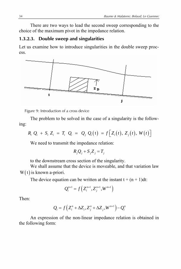
1.3.2.3. Double sweep and singularities
Let us examine how to introduce singularities in the double sweep proc-ess.
Figure 9: Introduction of a cross device
The problem to be solved in the case of a singularity is the follow-ing:
( ) ( ) ( ) ( ) t , , i i i i i i j i i jR Q S Z T Q Q Q f Z t Z t W t⎡ ⎤+ = = = ⎣ ⎦
We need to transmit the impedance relation:
j j j j jR Q S Z T+ =
to the downstream cross section of the singularity. We shall assume that the device is moveable, and that variation law is known a-priori. ( )W tThe device equation can be written at the instant t + (n + 1)dt:
( )1 1 1, ,n n ni i jQ f Z Z W+ + += 1n+
Then:
( )1 , ,n n ni i i j jQ f Z Z Z Z W Q+ n
i= + ∆ + ∆ −
An expression of the non-linear impedance relation is obtained in the following form:

SIC: A 1D HYDRODYNAMIC MODEL FOR RIVER AND IRRIGATION CANAL MODELING AND REGULATION 35 Capítulo 1
1 , ,n ni ij i j j j
i i
T RQ f Z Q Z Z W QS S
+⎛ ⎞⎛ ⎞∆ = + − ∆ + ∆ −⎜ ⎟⎜ ⎟⎜ ⎟⎝ ⎠⎝ ⎠
n ni
The problem is then to find the best possible linear approximation to this expression. The tangential approximation equation of the device variation law can be written as:
( )( ) ( )
( )
1
1 1
1
, ,
, , , ,
, ,
n n n ni i i i j j
n n n n n ni j i j i
i
n n ni j j
j
Q Q f Z Z Z Z W
ff Z Z W Z Z W ZZ
f Z Z W ZZ
+
+ +
+
+ ∆ = + ∆ + =
∂+ ∆ +∂
∂∆
∂
which leads to: j j j j jR Q S Z T+ =
with:
( )
j i j()R =S +R
()
() ()
i
j ij
nj i i i
i
fZfS SZ
fT T S f QZ
⎧ ⎫∂⎪ ⎪
∂⎪ ⎪⎪ ⎪∂⎪ ⎪= − +⎨ ⎬∂⎪ ⎪⎪ ⎪∂⎪ ⎪= + −
∂⎪ ⎪⎩ ⎭
This method cannot avoid the tangential approximation error of the device variation law created at each time step n, but counterbalances it in the next time step n+1. Indeed, a "correction wave" is included in the ex-pression of the coefficient in the form of an additive term
. jT
( )() - ni iS f Q
1.3.2.4. Network computation
Can the double sweep method be extended to a network of reaches inter-connected by nodes?
We will see that the double sweep method can be extended to tree-like network. There is no problem with a node with converging reaches. Continuity of discharges and water level equality allow computing the

36 Baume & Malaterre; Belaud; Le Guennec
coefficient of impedance relation in the upstream section of the reach leaving the node.
For diversion reaches at a node, it is necessary to know discharge repartition in each reach leaving the node to be able to proceed the first sweep.
1.3.2.4.1. Node modeling
A node can receive inflow discharges known hydrogram ( )aQ t (bound-ary condition). It can also loose discharges with a relation of the follow-ing form ( )f noQ Z for an offtake or a downstream rating curve.
A node can store water in a pool. This storage area is described by series of couple values (storage, level). The pool can loose water by evapotranspiration (speed of evaporation ( )epV t ) or seepage (speed of
seepage ) where ( )inf noV Z noZ is the pool level. At time t, the pool area A, the water level noZ , inflow discharges
and outflow discharges for reaches linked to the node are known. Writing continuity at note between time t and t
nQ 1Qt+ ∆ gives:
converging reaches diversion reaches
1
inf
. .
.( ).
no no
no
Z Z t t
no a nfZ t
t t
ep
t
dZ Q Q Q Q dt
V dt
+∆ +∆
+
+∆
⎛ ⎞= ∑ ∑ + −⎜ ⎟⎝ ⎠
− +
∑ ∑∫ ∫
∫
A
S V
Trapezium numerical integration of the above integral equation gives:
inf
inf
1
1inf1
inf1
2
02
low seepage converging diversionreaches reaches
low seepage converging reaches diversion reaches
k
k ka n epf
k
a n epf
tV V Q Q Q Q AV AV
t Q Q Q Q AV AV
+
+− −
− −
⎛ ⎞∆ ⎜ ⎟− − + + −⎜ ⎟⎝ ⎠
∆ ⎛ ⎞− + + −⎜ ⎟⎝ ⎠
∑ ∑ ∑ ∑
∑ ∑ ∑ ∑ =
kV being the pool volume at time k∆t. A linearized form of this equation is:

SIC: A 1D HYDRODYNAMIC MODEL FOR RIVER AND IRRIGATION CANAL MODELING AND REGULATION 37 Capítulo 1
seepage
converging reaches diversion reaches
1
inf( inf)2
02
kfk
no nono no no
n
Qt AA Z Z epZ Z Z
t Q Q
∂⎛ ⎞∆ ∂ ∂∆ + ∆ − + + +⎜ ⎟∂ ∂ ∂⎝ ⎠
∆ ⎛ ⎞− ∆ − ∆ =⎜ ⎟⎝ ⎠
∑
∑ ∑
VV V A (39)
The continuity of water level for reaches connected at the node al-lowed to replace the pool water level by the water level of the upstream section of a reach leaving the node or by the downstream section of a reach reaching the node.
1.3.2.4.2. Dentric network
nn
n
1
Figure 10: Dentric network of reaches
For each reach reaching the node, impedance relations are known:
n n n nr Q s Z tn∆ + ∆ =
That gives for all the reaches combining at the node:
n nn n
n n
s tQ Zr r
∆ + ∆ =∑ ∑ ∑
Water level equality at node gives another equation. In-deed, the upstream water level of the reach i1 leaving the node equal downstream water level of a reach i2 reaching the node:
( ) ( )1 k1 21
ki inZ Z
+ +=
1
or:
2 11 0 i i
n -Z Z =∆ ∆

38 Baume & Malaterre; Belaud; Le Guennec
12 2 2
n nn
i i in n
s tQ Zr r
∆ + ∆ =∑ ∑ ∑
so:
12 2
n nn
i i n n
s tQ Zr r
∆ = − ∆ +2i
∑ ∑ ∑
Discharge continuity at node (equation 39) stands for:
converging reaches
1 11 1 1
1
inf( inf)2
0 2
kf
n
Qt AA Z epZ Z Z
t Q Q
−∂⎛ ⎞∆ ∂ ∂
∆ + + +⎜ ⎟∂ ∂ ∂⎝ ⎠∆ ⎛ ⎞− ∆ − ∆ =⎜ ⎟
⎝ ⎠∑
VV V A Z∆
1
For the first section of the reach leaving the node:
1 1 1 1r Q s Z t∆ + ∆ =
With:
converging reaches
inflows seepage converging convergingreaches reaches
1
k
infinf1
1 11
1 inf1
2
( ) . 2
f nep
n
k
na n epf
n
tr
Qt s As A AZ r Z Z
tt t Q Q Q Q AVr
+ −
− −
∆=
⎛ ⎞∂∆ ∂ ∂⎜ ⎟= − ∑ − −⎜ ⎟∂ ∂ ∂⎝ ⎠
⎛ ⎞⎜ ⎟= ∆ + + − +⎜ ⎟⎝ ⎠
∑
∑ ∑ ∑ ∑
VV V
AV
If there is no pool and no inflow or seepage at node:
converging reaches
converging reaches converging reaches
1
1
11
1
.
n
nk
nn
n
r
ssr
tt Q Qr
=
=
⎛ ⎞= − +⎜ ⎟⎝ ⎠
∑
∑ ∑

SIC: A 1D HYDRODYNAMIC MODEL FOR RIVER AND IRRIGATION CANAL MODELING AND REGULATION 39 Capítulo 1
or:
converging reaches
converging reaches
1
1
1
1
.
n
n
n
n
r
ssr
ttr
=
=
=
∑
∑
1.3.2.4.3. Looped network
∆ Q 1 ? ∆ Q 1 ?
∆Q ∆ Q n
Figure 11: Looped network of reaches
To be able to compute the first sweep it is necessary to compute for diversion flows. To do so, the system of equation reduced to ex-
tremities of reaches is considered. The two equations 40 and 41 between two sections are condensed for each reach. To avoid numerical problems when the reach is very long these equations are written on a special form named normal form.
1Q∆
Discretisation between sections 1j = and 1 2j + =
1 22 2 12 2
22 2 2 11 2
(40)
(41)j=
j=
Q fe dZ ZQ Qb a cZ
∆ = ∆ + ∆ +
∆ = ∆ + ∆ +
Putting them to normal form:
40 Baume & Malaterre; Belaud; Le Guennec
21 2 2 21 2
2 22 2 2
2 2 2
(41) (41)
1 with , ,
j= j=Q Q Z
b ca a a
⊗→ ∆ + ∆ + ∆ =
= − = = −
U V W
U V W
1
( )1 2 22 21 1 1 2(41) and (40) j= j - -Q fe dZ Z Z⊗= → ∆ = ∆ + ∆ ∆ + +U V W2 2 2
( ) ( )
1 21 1 11
2 2 21 2 1 2 1 22
(40)
with , ,
j=Q Z Z
fd e d d
⊗∆ + ∆ + ∆ =
= = − − = +
U V W
U U V V W W
1
2
Discretisation between sections and 2j = 1 3j + =
2 33 3 23 3
33 3 3 22 3
(40)
(41)j=
j=
Q fe dZ ZQ Qb a cZ
∆ = ∆ + ∆ +
∆ = ∆ + ∆ +
Putting them to normal form:
( )( ) ( ) (
1 2 2
3 32 3 3 3 2 3 3 31 3 3
32 3 3 2 3 3 2 2 3 31 3
32 2 21 3
(41) , (41) and (40)
j= j= j=
b a c e d fQ Q QZ Za d b e c fQ Q Z
Q Q Z
⊗
⊗ ⊗ ⊗
→
∆ + ∆ + ∆ + + ∆ + ∆ + =
∆ + + ∆ + + ∆ = − +
∆ + ∆ + ∆ =
U V
U V V W
U V W
( )
)2
2
W
V
( )( )
( )( )
2
3 3 2 2 3 3 222 2 2
3 3 2 3 3 2 3 3 2
(41)
with
; ;
j=
b e c fa d a d a d
⊗
⊗ ⊗ ⊗+ − += = =
+ + +V W VU U V W
V V V

SIC: A 1D HYDRODYNAMIC MODEL FOR RIVER AND IRRIGATION CANAL MODELING AND REGULATION 41 Capítulo 1
=
1
( )
1 2 2
11 1
3 31 3 3 2 2 2 3 11
1 31 1 11
et(40) , (41) (41)
.
(40
j= j= j=
Q Z
e d - fQZ Z
Q Z Z
⊗ ⊗
⊗ ⊗
⊗ ⊗ ⊗
→
∆ + ∆ +
⎡ ⎤∆ + ∆ − ∆ + + =⎣ ⎦
∆ + ∆ + ∆ =
U
V U V W W
U V W
( ) ( )( )
2
1 1 3 2 1 1 1 3 3 2 1
1 1 3 3 3 2
)
with
, ,
j=
- d . e d
- f f d⊕
⊗
⊗ ⊗ ⊗ ⊗ ⊗
⊗
= = −
+ +
U U U V V V V W
W V W
etc... until section n. For all the reaches, this process gives:
11 11 nQ Z Z⊗ ⊗∆ + ∆ + ∆ =U V ⊗W
2
(42)
2 21 nnQ Q Z⊗ ⊗∆ + ∆ + ∆ =U V ⊗W (43)
This way to condense the Saint Venant equations avoids numerical problems.
1.3.2.4.4. Linear system for discharges predetermination at split flows
The reduce system can be written similarly to steady flow but now and are distinguished.
1Q∆
nQ∆
1 1
4
1 2
3
. = n
n
M A B Q CK I L Q CQ I F Z CN H I Z C
∆∆∆∆
(44)
In the first line of blocks the followings equations are stored: - Continuity equations at nodes that are not downstream node of network (including upstream boundary condition Q1(t)) blocks M, A, B and C1 (Equation 39),
- Upstream water level equality for reaches leaving a node, blocks B and C1 (Equation 21),

42 Baume & Malaterre; Belaud; Le Guennec
In the second and third line of blocks condensations equations (43) and (42) are stored.
In the forth lines of blocks the following equations are stored: - Downstream boundary conditions for the network in blocks I, C3 if Zn(t), if the downstream condition is a rating curve Qn(Zn), ∆Qn are eliminated by combination with equation (43) (block N appears),
- Water level equality at node between downstream section of a reach and upstream section of a reach connected at this node (blocks H, I, C3) (Equation 22).
Where: - I is unity matrix - K, L, Q, F are diagonal - H is upward triangular matrix with a nil diagonal
System (44) can be reduced to:
11
11 4 2 2 3
. . ( . . ) ( . )( . )
. . ( . . ) ( . ) ( . )
M A K B Q A L B F H Q N QH F I
C AC B C A L B F H C CH F I
−
−
⎡ ⎤− − + + − ∆ =−⎣ ⎦⎡ ⎤− − + + −−⎣ ⎦
The solution of this system gives the values ∆Q1 and so the up-stream impedance relation for the reaches.
1 11 11Q s tr Z∆ + ∆ =
With
1 1 1 11 , 0 , Qs tr = = = ∆
It is then possible to continue the first sweep.
1.3.2.5. Regulation modules
Automatic control of any structure (cross structures, offtakes, upstream or downstream boundary conditions) is possible inside SIC. The logic used to program this feature is based on the paper from Malaterre et al., 1998. It consists in defining separately the considered variables (meas-ured Z, controlled Y and control action variables U) and the control algo-rithm. This gives a tremendous power and flexibility in the different pos-sibilities offered. There is no limitation in the type of algorithm that can be developed and tested in the SIC software, from simple local PID con-trollers to complex non-linear multivariable controllers.

SIC: A 1D HYDRODYNAMIC MODEL FOR RIVER AND IRRIGATION CANAL MODELING AND REGULATION 43 Capítulo 1
First, the measured Z, controlled Y and control action variables U have to be specified. Some parameters can be specified concerning these variables (e.g. minimum gate movement, minimum and maximum val-ues, measure and control time step, etc.). Second, the design technique has to be specified. The most common techniques are already available (PID, BIVAL, ELFLO, interactive manual control, LTI discrete state space controllers, etc.). An open regulation module is given to the user, where any other type of control can be written in FORTRAN program-ming language. In addition, an interface with the commercial package MatLab16 through a DDE link (Dynamic Data Exchange) allows writing directly the regulation modules as a MatLab function, and using any MatLab function (included graphical functions). A SCADA (Supervisory Control and Data Acquisition) module is also available allowing control-ling a real canal. This SCADA module is very powerful since it can use any other regulation module of SIC (Figure 12). You can for example test regulation modules inside SIC in simulation mode and then switch to SCADA module using the same module without any rewriting work which removes error risks.
Figure 12: SCADA interface principle.
16 www.mathworks.com
44 Baume & Malaterre; Belaud; Le Guennec
Some auto tuning algorithms are also provided such as the ATV (Auto Tuning Variation) algorithm, which permits to calibrate automati-cally a PID controller. This allows users that are not specialists in control engineering to tune easily automatic control algorithms.
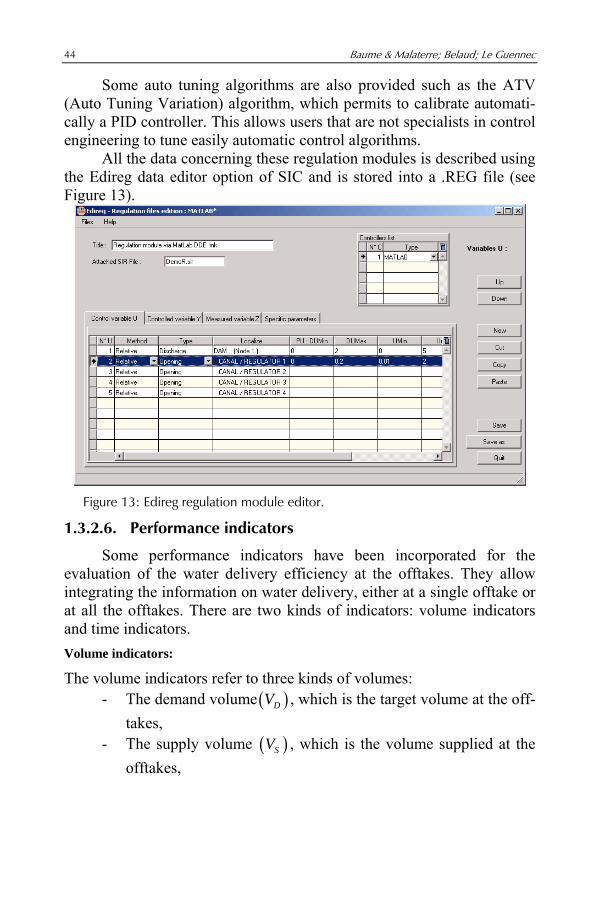
All the data concerning these regulation modules is described using the Edireg data editor option of SIC and is stored into a .REG file (see Figure 13).
Figure 13: Edireg regulation module editor.
1.3.2.6. Performance indicators
Some performance indicators have been incorporated for the evaluation of the water delivery efficiency at the offtakes. They allow integrating the information on water delivery, either at a single offtake or at all the offtakes. There are two kinds of indicators: volume indicators and time indicators. Volume indicators:
The volume indicators refer to three kinds of volumes: - The demand volume ( )DV , which is the target volume at the off-
takes, - The supply volume ( )SV , which is the volume supplied at the
offtakes,
SIC: A 1D HYDRODYNAMIC MODEL FOR RIVER AND IRRIGATION CANAL MODELING AND REGULATION 45 Capítulo 1
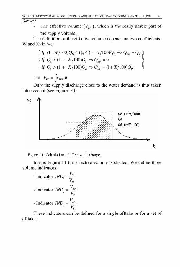
- The effective volume ( )EFV , which is the really usable part of the supply volume.
The definition of the effective volume depends on two coefficients: W and X (in %):
(1 100) (1 100) (1 100) 0 (1 100) (1 100)
D S D EF S
S D EF
S D EF
If W Q Q X Q Q QIf Q W Q QIf Q X Q Q X Q
− ≤ ≤ + => =⎧ ⎫⎪ ⎪< − ⇒ =⎨ ⎬⎪ ⎪> + ⇒ = +⎩ ⎭D
dt
and EF EF V Q= ∫ Only the supply discharge close to the water demand is thus taken
into account (see Figure 14).
Figure 14: Calculation of effective discharge.
In this Figure 14 the effective volume is shaded. We define three volume indicators:
- Indicator 1S
D
VINDV
=
- Indicator 2EF
D
VINDV
=
- Indicator 3EF
S
VINDV
=
These indicators can be defined for a single offtake or for a set of offtakes.

46 Baume & Malaterre; Belaud; Le Guennec
Time indicators
We define DT as the total period of time during which the demand dis-charge is non-zero and as the total period of time during which the effective discharge is non-zero. We introduce the indicator
EFT
4 EF DIND T E= It compares the duration of delivery of the effective vol-ume with that of the demand volume. This indicator is dimensionless and can only be calculated for individual offtakes since it doesn't have any significance for all the offtakes taken together.
We also define two time lags: 1T∆ and 2T∆ . 1T∆ is the time sepa-rating the start of the water demand and the start of the effective dis-charge. This time is positive if the effective discharge arrives after the demand discharge (Cf. Figure 15). 2T∆ is the time lag between the cen-ters of gravity of the demand hydrograph and the effective delivery hy-drograph.
Figure 15: Calculation of time lags.
All these indicators are defined for each offtake. They can be calcu-lated for any particular period of the simulation that the user wants to fo-cus on.
1.4. Sediment transport 1.4.1. Theoretical concepts
1.4.1.1. Basic equations for particle transport
Within reaches, one-dimensional transport is classically modeled by the convection-diffusion equation:

SIC: A 1D HYDRODYNAMIC MODEL FOR RIVER AND IRRIGATION CANAL MODELING AND REGULATION 47 Capítulo 1
( ) D
AuCAC CAKt x x x
∂∂ ∂ ∂⎡ ⎤+ − ⎢ ⎥∂ ∂ ∂ ∂⎣ ⎦= ϕ (45)
where A is the flow area, u the flow velocity, t the time, x the ab-scissa, C the particle concentration, defined as the ratio of the particle discharge to water discharge, KD the diffusion-dispersion coefficient, ϕ the exchange rate. In the following, the particle concentration will be ex-pressed in kg/m3, ϕ is therefore in kg.m-1.s-1.
In steady state, the terms ∂/∂t disappear. A dimensional analysis shows that diffusion can be neglected as well and equation 45 simplifies as:
AuCx
∂= ϕ
∂ (46)
In unsteady state, especially for pollution peaks, diffusion can be significant and the second order derivative cannot be neglected.
1.4.1.2. Model of exchange term
1.4.1.2.1. Solute transport
The exchange term represents the flux (mass per unit time and unit length) of material brought to the flow. For solute transport, it stands for adsorption, desorption or any chemical reaction. For example, the first-order degradation reaction, such as auto-epuration process in riv-ers, writes as follows:
.dC k Cdt
= − (47)
where k is the reaction constant. The above equation develops as:
.C Cu k
t xC∂ ∂
+ = −∂ ∂ (48)
and the corresponding degradation rate would be written as
. .k A Cϕ = − .
1.4.1.2.2. Sediment transport
For sediment transport, the exchange rate is rather more complicated. In uniform channels, this flow rate is supposed to reach a sediment transport capacity *
sQ . Many formulae have been developed to assess this quantity

48 Baume & Malaterre; Belaud; Le Guennec
such as Meyer-Peter (1948), Einstein (1950), Bagnold (1966), Engelund-Hansen (1967), Ackers-White (1973), Van Rijn (1984) etc. Though none has become universal and reliable enough to avoid calibration on field data. Anyhow, all these formulae shows a strong correlation between the sediment transport capacity and the non-dimensional shear stress (or
Shields parameter), *
( )h
s
R Jd
ρτ =
ρ − ρ, in which Rh represents the hydraulic
radius, J the hydraulic gradient, ρ the water density, ρs the sediment den-sity and d the sediment representative size (generally the medium diame-ter).
If the sediment input in a reach is superior to the sediment transport capacity, there should be deposition. If it is inferior, there should be ero-sion. For fine sediments transported in suspension, the adaptation to the equilibrium state may not be immediate. The non-equilibrium model states that:
*1 (s )s sA
Q Q Qx L
∂ϕ = = −
∂ (49)
where AL is the adaptation length. The expression of AL can take into account the role of the viscosity, the particle diameter and the turbu-lence such as:
*
AuLw
= α (50)
α is a parameter, the shear velocity (characteristics of the flow) and w the fall velocity of the particles.
*u
The fall velocity is estimated by the empirical formula:
0.53
2
0.01( 1)10 1 1s gdwd
⎛ ⎞⎛ν −⎜⎞
⎟= +⎜⎜ ⎟ν⎝ ⎠⎝ ⎠−⎟ (51)
When several classes are transported, the total sediment transport capacity can be calculated as a combination of the sediment transport ca-pacities, calculated with the representative diameters of each class and weighed by proportion of each class in the total material.
Cohesive sediment transport should also take into account floccula-tion properties (which depend on the particle nature, the concentration and the salinity). Bed consolidation may also reduce the erosion capacity.

SIC: A 1D HYDRODYNAMIC MODEL FOR RIVER AND IRRIGATION CANAL MODELING AND REGULATION 49 Capítulo 1
Another classical way to express the exchange rate is to consider it as proportional to the difference between the actual shear stress ( ) and critical shear stresses, possibly different for erosion and deposition.
0 gRJτ = ρ
1.4.1.3. Junctions
1.4.1.3.1. Mass conservation
The first principle is the mass conservation at each node of the model. For a convergent system, this principle is sufficient for the complete resolution:
3 1 1 2 2 1 2( . . ) /( )C Q C Q C Q Q= + + (52)
Where 1 and 2 designate upstream channels and 3 the downstream channel.
For divergent systems (1 2 and 3), the simplest assumption is C2=C3=C1, which is generally verified as far as solute or very fine parti-cles (like clay of fine silt) are concerned, but not for coarser particles. Indeed, measurements conducted in channels and numerical experiments have shown a dependence of the concentration in offtakes with the sedi-ment distribution in the flow and the offtake geometry:
offtake
offtake canals s canal
QQ QQ
= θ (53)
in which θmay be different from 1, particularly for sand. If not known, θ can be estimated thanks to a model using typical sediment and velocity distributions in cross sections and the offtake geometry. This approach represents well: - The influence of the offtake opening compared to the canal depth;
- The influence of the offtake discharge compared to canal discharge (an offtake with a low discharge will take water flowing near the banks).
1.4.1.3.2. Velocity distribution
Vertically, the velocity distribution is assumed to follow a power law:
( ) ( ) 1/ auu z A z h=
With a1 between 0 and 1 (typically around 0.2).

50 Baume & Malaterre; Belaud; Le Guennec
Horizontally, the distribution is assumed to be a power function as well:
( ) max2 | |1 yu y u
b
γ⎛ ⎞⎡ ⎤= −⎜ ⎟⎢ ⎥⎜ ⎟⎣ ⎦⎝ ⎠ (54)
With γ >1 (higher than 4 practically). Finally, the velocity distribution can be obtained from the mean veloc-
ity by:
( ) ( ) 1 2, 1 1z yu y z Uh b
β γ⎡ ⎤γ + ⎛ ⎞= β + −⎢ ⎥⎜ ⎟γ ⎝ ⎠ ⎢ ⎥⎣ ⎦ (55)
1.4.1.3.3. Concentration distribution
The approach of Rouse (1937) remains a reference as far as concentration profiles are concerned. The vertical distribution writes as follows:
.mC h z
C z hε
− ε⎛= ⎜⎞⎟− ε⎝ ⎠
(56)
With:
ε : Reference level (limit height between bed-load and suspended load)
Cε : concentration at this level
m : exponent, originally defined as wmu∗=
ακ, κ Von Karman constant, α
ratio between ∈s (vertical diffusion coefficient) and ∈m (turbulent viscosity), u* shear velocity. A value of α.κ = 0.4 is usual. Practically, ε (bed load layer thickness) is uneasy to determine and much lower than h.
With ε/h <<1, equation 45 writes:
( ) .m
Ch zC z A
z−⎛= ⎜
⎝ ⎠⎞⎟ ()
Where ( ) mCA C h= ε .
The transverse distribution is supposed to be of the same type as the velocity one, with possibly a different exponent.

SIC: A 1D HYDRODYNAMIC MODEL FOR RIVER AND IRRIGATION CANAL MODELING AND REGULATION 51 Capítulo 1
1.4.1.3.4. Influence zone of the offtake
Then the zone of the cross section where the water flows from is defined using the offtake geometry:
Watercoursez
z
z
z
z
water
beddown
sill
up
roof
z
Figure 16: sediment diversion model.
zup and zdown are assumed to be linked by the following relations:
( )( )
down sill vi sill bed
up roof vi water roof
z z z z
z z z z
= −α −
= −α −
Where αvi is a parameter. The value ymax is defined so that the discharge flowing in the zone
delimited by the offtake bank, ymax , zup and zdown equals the discharge off-take.
1.4.1.4. Bed evolution
Bed aggradation or degradation is obtained by conservation equations. The exchange rate represents the material lost by the bed and equals
( )1sSpt
∂ϕ = −ρ −
∂ (58)
Where ρs is the sediment density (kg/m3), p the porosity and S the bed area. The conservation equation can be written for several classes of particles. Nevertheless, in case of erosion, the exchange rates of the dif-ferent classes are linked by the bed grain size distribution.
For deposition, deposits are made in the lowest parts (producing a horizontal bed at the cross section bottom), or proportionally to the water depth (directly linked to the quantity of particles available in the flow) (Figure 17).
For erosion, it is stated that the variation in a vertical is propor-tional to the water depth in this vertical (distribution 1).

52 Baume & Malaterre; Belaud; Le Guennec
y
zdS dS
distribution 1 distribution 2 Figure 17: sediment deposition pattern.
1.4.2. Numerical aspects
In both steady and unsteady flow calculations, particle transport is calcu-lated at each time step after the hydraulic calculation.
1.4.2.1. Steady flow
The concentration field is calculated in the network from upstream to downstream. The bed evolution is calculated afterwards and the new ge-ometry is used for the flow calculation at the next time step. The main stages of the sediment calculation, at each time step, are presented below.
1.4.2.1.1. Sediment diversion at nodes
Several models are available to calculate θ for each transported class and each node:
o θ is known: its value is fixed
o θ is unknown: its value is set to 1 (same concentration in offtake and parent channel)
o θ is unknown but the values of θ for the other offtakes linked to the same node are known; then θ is calculated by mass conservation
o θ is calculated thanks to the diversion model presented before.
In this model, the velocity and concentration fields, u(x,y,z) and C(x,y,z), are calculated first from mean values (U and C). The zone of influence of the offtake, delimited by the two values , of y is calcu-lated by numerical integration.
1y 2y
1.4.2.1.2. Calculation in a reach
The sediment transport capacity is calculated first in the calculation sec-tions i. It only depends on the hydraulic, geometric variables and the sediment properties. The adaptation length is calculated as well.

SIC: A 1D HYDRODYNAMIC MODEL FOR RIVER AND IRRIGATION CANAL MODELING AND REGULATION 53 Capítulo 1
The next step consists of the resolution of the non-equilibrium transport equation, written with concentrations:
(1
A
C C Cx L
∗ )∂= −
∂ (59)
The adaptation length and the sediment transport capacity C* are approximated by their averages between calculation sections i and i+1. Then, the solution is an exponential function:
[ ]1; ,i ix x x +∀ ∈ ( )( ) ( ) * ( )i
A
x xL
i iC x C x C C x e−
−= + − (60)
And the value of Ci+1 is calculated knowing the concentration Ci.
When several classes are transported, the total sediment transport capacity is calculated as follows:
(61) ( ), 1
1
tNj i j
ij
C p C d∗ − ∗
=
=∑
Where ,j ip is the proportion of sediments in class j (transported particles) in section i,
the number of transported classes, tN jd the representative diameter for class j. The adaptation length is calculated for each class as well:
*
,j i
A i j
uLw
=α
(62)
with jw settling velocity for class j.
Then :
( *1jj
jA
dC )jp C Cdx L
= − (63)
The availability of fine sediments in the bed can be a limitation for erosion. A correction factor F is estimated:
* '
' 11..
* '
' 1
min
jj
jj N j
j
j
F ==
=
ϕ=
ϕ µ
∑
∑ (64)
Then erosion/deposition rate *,j j
i F iϕ = µ ϕ in each calculation section. Concentra-tions are corrected if necessary:
54 Baume & Malaterre; Belaud; Le Guennec
( ) (1 1 1 1*
ji
i i i i i i i ij wti
Q C Q C Q C Q C+ + + +
ϕ− = −
ϕ) (65)
With potential erosion rate, subscript indicates the values without test. * ,j iϕ ()wt
The model allows taking this phenomenon into account if the active layer option is se-lected. In this case, the eroded particles are in the same proportion as in the bed.
1.4.2.1.3. Bed evolution
In section i, the bed variation during time t-dt and time t in given by (continuity equation):
( )*
,1 1i
i i i iA i
Qdt dtdS C C C Ip p L i i
⎡ ⎤= − ϕ = − − +⎢ ⎥
− − ⎢ ⎥⎣ ⎦ (66)
Where iI is the seepage rate at section i. However, discontinuities may appear at nodes. Indeed, the previous equation is not supposed to give the same variation in the upstream section and the downstream sec-tion of a node, whereas both are at the same location. A procedure calcu-lates the bed variation at this location as a weighed average of the up-stream and downstream bed variation; the total deposited or eroded vol-ume is conserved. This procedure allows dividing a reach in two reaches without changing the simulated bed evolution.
1.4.2.1.4. Bed size distribution
This option is available if the active layer option is selected. The bed composition is unchanged if there is erosion. In case of deposition, the bed composition results from the composition in the active layer at time t plus the deposition during t and t+dt. The active layer is defined by its thickness and its width given by the user.
1.4.2.1.5. Numerical stability
Instability can result from high values of the ratio dt/LA. Indeed, if the adaptation length is short, the concentration adapts quickly to the sedi-ment transport capacity and the spatial variations (in the concentration field) may be significant; this can result, in a time step, into a high bed variation. The time step should be of a few days for an adaptation length of one kilometer. In any case, the bed modification at each time step should not modify too much the hydraulic conditions.

SIC: A 1D HYDRODYNAMIC MODEL FOR RIVER AND IRRIGATION CANAL MODELING AND REGULATION 55 Capítulo 1
1.4.2.2. Unsteady flow calculation
The same formulae as for steady flow are used but the convection-diffusion equation is solved in its whole.
A Holly-Preissmann scheme is used for the convective part. This algorithm uses the method of characteristics. The transport-diffusion equation is written along the trajectory:
dC Udx
= (67)
The method consists of the determination of the position P which had a particle at time t-dt and arrived in M at time t:
*( ) ( , ) .M
n
P
C M C P t dt= + ϕ∫ , where ϕ is the source term and C*(M)
= C(M,tn+1) with only convection. The integration along the trajectory is made with a Range-Kutta method.
Figure 18: characteristics method.
There are several ways to obtain C(P). The Holly-Preissmann method (default method in SIC) allows to simulation sharp pollution peaks with little numerical diffusion. Its main drawback is the calculation time. The simplified Holly-Preissmann method is much quicker but in-volves more diffusion.
The diffusion terms are obtained by writing that the difference
C(M,tn+1) and C*(M) equals the diffusion term DCAK
x x∂ ∂⎡ ⎤⎢ ⎥∂ ∂⎣ ⎦
. This equa-
tion is solved with a Crank-Nicholson method.

56 Baume & Malaterre; Belaud; Le Guennec
This scheme allows simulating pollution peaks. Sediment transport is calculated from upstream to downstream at each hydraulic time step, but, since the bed variations are slow, the geometry is saved at longer time steps. The geometry is updated at the time step used for the steady flow. The time step selected then is so that the hydraulic variables are approximated well.
Inverse currents (due to tides, for example) can be simulated as well.
1.4.3. Model application
1.4.3.1. General
Due to the poor reliability of the sediment transport and diffusion-dispersion formulae, the models should be compared and calibrated with field data, whenever possible. For design, however, actual data cannot be used for verification. The use of the result in a relative way (comparison between simulations) is preferable to the use of absolute results. A sensi-tivity analysis is highly recommended as well.
In order to illustrate the role of various parameters, simulations are performed on a test canal. It consists of two reaches in series with an off-take at their junction. The canal is a 10m wide rectangular channel with a slope of 0.4‰.
Figure 19 illustrates the variability that can be obtained through the choice of the sediment transport formula among 7 classical formulae.
The adaptation length can be adjusted with α coefficient. Figure 20 shows the influence of this coefficient on the bed evolution. One can see that the bed aggradation is quicker, although the equilibrium profile is the same, independently on the erosion-deposition rates.

SIC: A 1D HYDRODYNAMIC MODEL FOR RIVER AND IRRIGATION CANAL MODELING AND REGULATION 57 Capítulo 1
Sediment transport capacities - C*
0
0.2
0.4
0.6
0.8
1
1.2
1.4
0 5 10 15 20Discharge (m3/s)
Equi
libriu
m c
once
ntra
tion
(kg/
m3) EH
AW
BG
VR
KK1
YG
KK2
Figure 19 : comparison of the sediment transport formula (C* versus discharge) – EH: Engelund-Hansen (1967); AW: Ackers-White (1973); BG: Bagnold (1966); VR: Van Rijn (1984); KK1: Karim-Kennedy (1981); YG: Yang (1973); KK2: Karim-Kennedy (1990)
C a na l 2
8.0
8.5
9.0
9.5
10.0
10.5
11.0
11.5
0 50 100 150 200 250 300 350 400
t (days )
a lpha=0.01, X=0alpha=0.01, X=2kmalpha=0.01, X=5kmalpha=0.05, X=0alpha=0.05, X=2kmalpha=0.05, X=5km
Figure 20 : influence of the deposition parameter α. The incoming
concentration is 0.5kg/m3 and the flow rate 5m3/s. The equilibrium concentration, calculated with Engelund-Hansen formula.

58 Baume & Malaterre; Belaud; Le Guennec
1.4.3.2. Indicators
A few indicators can be calculated for the evaluation of particle transport processes and design, maintenance and operation strategies: shear stress long profile, which is a precious indicator for characteriz-
ing sediment transport processes; sediment or solute concentrations (with respect to time and distance); deposited volumes in reaches; modifications on bed and water elevations; delivery performance ratios (actual discharge divided by design dis-
charge) and their evolution; coefficient of variation of the delivery performance ratios.
Most indicators are relevant when calculated after a period long enough to generate significant bed modifications. Typically, scenarios should last from a few months to a few years.
1.4.3.3. Design
The model can be used for pre-design applications, such as: efficiency of sediment control devices on sediment behavior in a sys-
tem (desilting basins, sediment excluders, sediment extractors); size and position of offtakes; Relative influence of channel characteristics on sediment transport.
Civil engineering aspects are not tackled within the software.
1.4.3.4. Maintenance
Maintenance is carried out in irrigation systems, sewers or rivers. These operations consist of the resizing of the channel or the excavation of a given amount of sediment. The performance of the maintenance strate-gies according to one or several indicators can be optimized. SIC allows testing different maintenance strategies.
1.4.3.5. Real-time operation
Operations strategies can result in very different hydraulic behaviors, and therefore in very different sediment behaviors. In irrigation canals, for example, a same water volume can be supplied through a proportional distribution or a rotational schedule. Both strategies largely differ in terms of discharge and water levels at control gates, therefore in terms of particle transport.
SIC: A 1D HYDRODYNAMIC MODEL FOR RIVER AND IRRIGATION CANAL MODELING AND REGULATION 59 Capítulo 1
1.4.3.6. Sediment balance
A sediment analysis can be conducted at different degrees of complexity. In watersheds, the sediment balance is generally the first step of the analysis. The model is a helpful for:
- calculating the dilution effects;
- assessing the importance of exchange terms (erosion or deposition, solute degradation, inflows or outflows);
- evaluating the transit times;
- Evaluating the load from partial measurements.
1.5. Example 1.5.1. ASCE Test
In order to have an idea on the computational accuracy of the model, and to compare different models, two tests have been carried out on the SIC model as suggested by the ASCE Task Committee on hydraulic simula-tion. The conditions of these two tests are described in the paper from (Contractor et al., 1993). The results obtained by other softwares on the same tests are presented in the same issue of the ASCE Journal of Irriga-tion and Drainage Engineering.
1.5.1.1. Mass Conservation Test
The first test consists in imposing a 1-period sinusoidal discharge Q=200 sin(2πt/21600) for 0≤t≤6h and Q=0 for t>6h at the upstream end of a 10 km long horizontal canal. Its cross section is trapezoidal with a base width of 10 m and a side slope of 2. The canal is closed at its downstream end. Its initial discharge is 0 m3/s and initial depth is 7 m. The simulation was made with the usual SIC parameters: θ = 0.6 and no iterations. If the results are given in centimetres, the new water elevation all over the canal (after stabilisation) is 7.04 m, corresponding to an error of:
• 0.57 % in terms of water elevation • 0.91 % in terms of volume
If the results are given in millimetres, the new water elevation all over the canal (after stabilisation) is 7.043 m, corresponding to an error of:
• 0.61 % in terms of water elevation • 0.97 % in terms of volume

60 Baume & Malaterre; Belaud; Le Guennec
With more than 1 iteration (non-linear calculation) the error is nil.
1.5.1.2. Test With Ramp Discharge as Inflow
The second test consists in imposing a ramp discharge inflow at the up-stream end of a 3.219 km long canal. Its cross section is trapezoidal with a base width of 9.144 m and a side slope of 2. The canal longitudinal slope is 1 in 2000. The canal is at normal depth at its downstream end. Its initial discharge is 28.32 m3/s and initial depth is 1.707 m. Flow increases linearly from 28.32 m3/s to 141.6 m3/s in 10 minutes and then stays con-stant. For a time step of 10 minutes, some deviations can be seen, compared to the "USM solution", but not really oscillations. For smaller time steps (2 and 1 minutes), the accuracy is very good. Comparison of model outputs for the different time steps are presented in the following graph:
Figure 21: SIC results on the ASCE ramp discharge test.
1.5.2. Automatic regulation f an irrigation canal
The SIC software has been used to design irrigation canals and their manual or automatic control devices and procedures for more than hun-dred canals all over the world. This has been done mainly by Consulting Companies using SIC, but also by Cemagref, National or International Research centers and all the SIC users.

SIC: A 1D HYDRODYNAMIC MODEL FOR RIVER AND IRRIGATION CANAL MODELING AND REGULATION 61 Capítulo 1
In this chapter, we illustrate part of the possibilities offered by SIC to design, tune and test automatic controllers on irrigation canals. We will use in particular the ATVPID regulation module allowing to tune automatically a PID (Proportional – Integral – Derivative) controller by the ATV (Auto-Tune Variation) method, and the SCADA regulation module allowing to do this directly on a real canal, and not only in nu-merical simulation mode.
The experiments presented hereafter are performed on the Gignac canal, located 40 km north-west of Montpellier, south of France. The main canal is 50 km long, with a common feeder (8 km long from the intake in the river to the Partiteur device) and two branches on the left and right banks of the river (respectively 27 and 15 km long). The canal is concrete lined, with a rectangular cross section on the feeder and a trapezoidal one on the branches, with average slopes of respectively, 0.35 and 0.50 m/km. The design flow of the canal is 3.5 m3/s. The canal has been equipped with sensors, actuators and a SCADA system, which en-ables the monitoring and control of four reaches in a row on the feeder above Partiteur cross-regulator and the right bank branch from Partiteur to Mas Rouvière cross-regulator. A longitudinal view of the feeder and the right bank branch is depicted in Figure 22 (generated by SIC steady flow result module).
Figure 22: Gignac Canal (bed, bank and water elevations).

62 Baume & Malaterre; Belaud; Le Guennec
Figure 23: Gignac Canal (discharges).
This canal is composed of a feeder canal, and two branches: a left branch of 30 km, with a design flow of 1 m3/s and a right branch of 25 km, with a design flow of 2.5 m3/s (see Figure 23 for a simple example of discharges along the canal). The right branch is composed of 4 pools separated by controlled cross devices, 150 offtakes, 13 gates and 15 weirs. The SIC_SCADA interface of SIC is getting about 200 data values in real-time from sensors and local Programmable Logic Controllers (PLC) along the canal. The acquisition time step can be selected down to a few seconds. Some of the gates, sensors and actuators have been in-stalled by Cemagref and the manager (ASA de Gignac), with the finan-cial help of Région Languedoc-Roussillon, Agence de l'Eau Rhône Méditerrannée Corse, and Département de l'Hérault, in the context of a scientific project initiated in 2002.
A SCADA system has been developed and installed for the Gignac canal. A graphical interface of the SCADA system allows visualizing, in real time, the hydraulic state of the canal as illustrated on the Figure 24. The SCADA interface also allows defining some parameters such as the data acquisition time step.

SIC: A 1D HYDRODYNAMIC MODEL FOR RIVER AND IRRIGATION CANAL MODELING AND REGULATION 63 Capítulo 1
Figure 24: SCADA screen of the Gignac Canal.
The SCADA system is also providing real time measurements (through the data.txt file) to the SIC_SCADA interface and sending gate position targets in real time (through the csg.txt file) as described in Figure 12.
The type and location of the measured variables Z, the type and lo-cation of the control action variables U and the control algorithm are de-fined using the regulation module interface as illustrated Figure 25. In this example we use the ATVPID regulation module. This algorithm is automatically tuning a PID (Proportionnal, Integral, Derivative) control-ler using the ATV (AutoTuning Variation) method (Skogestad et al., 1998, Georges et al., 2002). After the relay experiment allowing to com-pute the PID coefficients, the PID controller is switched on automati-cally. This method is very powerfull and usefull since any PID controller can be installed and tuned with no requirement in control engineering knowledge. An additionnal feature of the example presented here is that this calculation is done directly on the real canal and not only in numeri-cal simulation. The SIC_SCADA interface displayed on the screen dur-ing the calculation is presented Figure 26. It allows to visualize the ex-change of data between SIC and the Gignac canal.

64 Baume & Malaterre; Belaud; Le Guennec
Figure 25: SIC interface for the edition of the regulation module.
Figure 26: SCADA_SIC interface.
The example presented here consists in designing and testing a lo-cal downstream PID controller, where the control action variable U is the gate opening at the Partiteur left branch head gate and the measured vari-able Z is the water level downstream of this gate. We can observe, on Figure 27, that the relay test has been carried out during 10 minutes cor-responding to 4 oscillation cycles as specified and that the calculated PID has been then switched on (Kp=0.6, Ti=96s). Then, a change in the con-

SIC: A 1D HYDRODYNAMIC MODEL FOR RIVER AND IRRIGATION CANAL MODELING AND REGULATION 65 Capítulo 1
trolled downstream water level Z has been imposed at time 13:26 (from 67 to 91 cm) and we can observe that the controller does a good job, moving the gate opening in order to reach this new target.
Figure 27: SCADA outputs screen of the Gignac Canal.
1.5.3. Application to the Amazonian hydrographic network
In the context of the HyBam17 program, the 1D unsteady flow hydrody-namic model SIC has been used to simulate the flows in the drainage network of the Amazon basin (Baume et al. 2003). Hydrodynamic mod-eling has first been realized from the Manacapuru (Rio Solimões), Moura (Rio Negro) and Vista Alegre (Rio Madeira) downwards to Obidos (Rio Amazon).
17 http://www.mpl.ird.fr/hybam/

66 Baume & Malaterre; Belaud; Le Guennec
Rio Amazonas
Rio Negro
Rio Madeira
90 0 90 180 km
Manacapuru
Moura
Faz. Vista Alegre
Óbidos
Figure 28: Modeled reaches.
The length of the reach from the Manacapuru down to Obidos is about 700 km, with a mean slope of water level of about 2.10-5 m/m. The discharges in Obidos are about 75 000 m3/s during the low water period and 260 000 m3/s at high water.
1.5.3.1. Available data
Water level, discharge, altimetry and bathymetry data have been col-lected from existing sources (Water National Agency, IBGE, HiBam Program, DHN, CPRM)
Bathymetry: Maps from the “DHN” (Directorate of Hydrography and Navigation – Brazilian Navy) were used and measurement cam-paigns allowed to collect cross sections with a step of 60 km (example presented here) and of 10 km (now available, but not yet used).
These campaigns were performed at different periods of the hydro-logic cycle on the rivers, including measurements of cross-sections, bed levels, hydraulic discharges and velocity profiles using ADCP, but they are limited to the minor-medium bed of the rivers. The water discharges at the different stations were thus quantified, and the local and lateral in-flows specified.

SIC: A 1D HYDRODYNAMIC MODEL FOR RIVER AND IRRIGATION CANAL MODELING AND REGULATION 67 Capítulo 1
Multiple sources topographic data of the water surface levels were used to state as precisely as possible the free surface flows.
Bed level and 3 free surface flows levels from Manacapuru (0 km) downstream to Obidos (722 km)Altimetric leveling using "corrected" IBGE network or GPS positionning
+ EGM96 geoid mode
-100
distance from Manacapu
-80
-60
-40
-20
0
20
40
0 100 200 300 400 500 600 700 800
ru (km)
leve
ls (m
) res
pect
ed th
e m
ean
sea
leve
l
Bed level147 000 m3/s262 000 m3/s93 200 m3/s
additional lateral discharges estimated using
scharge relationship in Obidos is the downstream ms of hysteresis for the higher val-
dynamic model has been realized in steady state to de
For all reaches, roughness proved to de-
Figure 29: Bed level and free surface flows.
1.5.3.2. Boundary conditions
Upstream conditions of the modeling are the discharges at the three nodes Moura, Manacapuru and Vista Alegre, during the years 1995-1999 (five hydrological cycles), with
a simplified method based on the conservation of fluxes and some rainfall-discharge relationship.
The stage-diboundary condition, with some probleues of discharges.
1.5.3.3. Calibration of the model
Calibration of the hydrotermine roughness coefficients, and unsteady state to estimate the
geometry of major bed. Steady state calibration took into account the minor bed section,
making the assumption that there was no longitudinal flow in the major bed. Manning roughness coefficients were then computed in order to match observed water profiles.

68 Baume & Malaterre; Belaud; Le Guennec
crease
ed by the model without major bed, it is possib
lood plain extents, as shown in Figure 33 (Active microwave remotely sensed JERS-1 images provided by the Global Rain Forest Mapping).
with increasing river stage (water level or discharge). The Man-ning coefficient is around 0.03
Flooding areas and major bed are estimated by fitting the observed and computed flood hydrographs. Comparing the observed outflow at Obidos with the outflow calculat
le to quantify the volume stored in the major bed for different river stages and the associated width.
Unfortunately, the geometry of these flooded areas is not well known. The concept of a lateral storage major bed, along the reaches, as schematized in Figure 32, is efficient but not necessarily representative of the actual f
Observed and calculated hydrographs in Obidos
0
50000
100000
150000
200000
250000
300000
1/1/1995 7/20/1995 2/5/1996 8/23/1996 3/11/1997 9/27/1997 4/15/1998days
11/1/1998 5/20/1999 12/6/1999
Dis
char
ges
(m3 /s
)
observed without major bed
Figure 30: Outflows in Obidos, without major bed..

SIC: A 1D HYDRODYNAMIC MODEL FOR RIVER AND IRRIGATION CANAL MODELING AND REGULATION 69 Capítulo 1
-40000
-30000
-20000
-10000
0
10000
20000
30000
40000
1/1/1995 1/1/1996 1/1/1997 1/1/1998 1/1/1999
Days
Dis
char
ge (m
3/s)
Stored DischargeReleased Discharge
Figure 31: Use of the hydrographs above to quantify the stored and released
discharges.
Figure 32: Scheme of minor, medium and major beds and their contribution
to flow and storage.
Figure 33: Map of flooded areas using satellite remote sensing.

70 Baume & Malaterre; Belaud; Le Guennec
Observed and calculated hydrographs in Obidos
0
50000
100000
150000
200000
250000
300000
1/1/1995 7/20/1995 2/5/1996 8/23/1996 3/11/1997 9/27/1997 4/15/1998 11/1/1998 5/20/1999 12/6/1999
days
Dis
char
ges
(m3 /s
)
observed with major bed
Figure 34: Outflows in Obidos, with major bed.
1.5.3.4. Sediment transport model
SIC Sedi, the sediment transport module coupled to the hydrodynamic model SIC, allows simulating the sediment dynamics along the river.
In the first instance, the model of sediment transport between Manacapuru and Obidos is built on the available in situ measurements. They are obtained by sampling every ten days the suspended flow just under the free surface and so concern only the finer particles of the sus-pended load. In Obidos, d50 = 18 µm, d85 = 58 µm.
1.5.3.5. Modelling
The hydrodynamic model computes all hydraulic variables. For given solid particles this allows to determine the capacity of the river to trans-port suspended sediments. In the formalism of Bagnold, this capacity is linked to the shear stress and the sediment fall velocity.
To treat the transport solid under non-equilibrium conditions, the loading law of Daubert-Lebreton is used in its general form.
The data needed for the boundaries conditions are here the sus-pended load in the three upstream contributors (Rio Negro, Solimoes and Madeira). They are estimated by multiplying the concentrations of sus-pended matter near the free surface by the mean discharge in the cross section. The solid discharges in Vista Alegre (Madeira) and Manacapuru

SIC: A 1D HYDRODYNAMIC MODEL FOR RIVER AND IRRIGATION CANAL MODELING AND REGULATION 71 Capítulo 1
(Solimões) are presented Figure 35. In the Rio Negro, the solid discharge is very low.
0
5
10
15
20
25
30
35
40
1/1 31/1 2/3 1/4 1/5 31/5 30/6 30/7 29/8 28/9 28/10 27/11 27/12day
Sol
id D
isch
arge
(ton
/s)
Vista Alegre
Manacapuru
Obidos
VA
Ma
Ob
Solid discharges in Vista Alegre (Madeira) , Manacapuru (Solimoes) and in Obidos (Amazon)
Figure 35: Observed solid discharges (Suspended load, 1999).
If we consider the sum of the entrances (Vista Alegre + Manacapuru), the balance with the observed suspended load in Obidos presents a deficit. A third of the suspended load is missing!
Here, the solid particles are fine, the unit power and the turbulence level of the Amazon River are high, but despite these conditions, a de-posit would occur. Another problem here is the role of the flooded areas, or varzeas, which are assumed to store part of the flood, but work also as a sediment trap.
1.5.3.6. First results
The total solid volume over one year is respected, but the calculated dis-charges are lower than the observed ones for the months of January and February which correspond to the first part of the increasing flood, before the overbank flows. That seems to be due to a too low transport capacity: in the model, some deposits can occur in the upstream reaches whereas this does not exist in the field.
The actual unit stream power of the Amazon River is perhaps higher than the formula predicts, due to the presence of bed forms, boils, which make the re-suspension easier

72 Baume & Malaterre; Belaud; Le Guennec
Simulated and measured solid discharges in Obidos in 1999
0
5
10
15
20
25
30
35
01/01/99 31/01/99 02/03/99 02/04/99 02/05/99 02/06/99 02/07/99 01/08/99 01/09/99 01/10/99 01/11/99 01/12/99 01/01/00
day
Qs
(ton/
s)
Figure 36: Computed and observed suspended load.
1.5.4. Irrigation system, Pakistan
1.5.4.1. Context
The example presented here is a secondary irrigation system, Sangro Dis-tributary, located in South Pakistan (Sindh province). The canal is 16km long with a head design discharge of 3m3/s and comprises 2 branches, Jarwari and Chahu minors, around 8km long each. The whole system ir-rigated 7,500ha thanks to 60 irrigation outlets spread along the system (APM and open flumes). In the upstream part, its bed is now 1 m higher than designed in 1960. One branch has to be desilted frequently to pre-serve its conveyance capacity. The maintenance of this system suffers from money and machine restrictions.
The canal is operated at its full supply level if water is available. There are closures according to a rotation schedule when water is scarce at Jamrao Canal head.
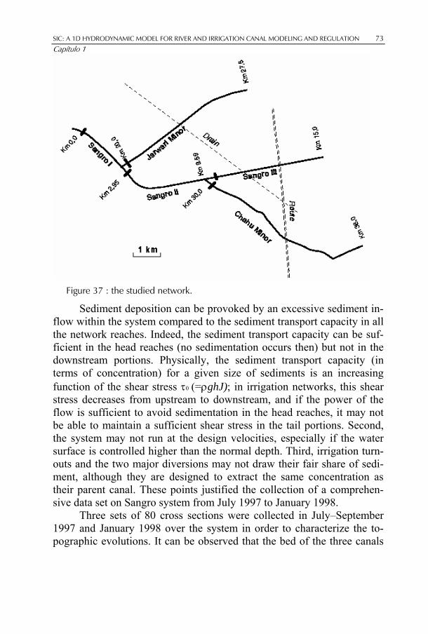
SIC: A 1D HYDRODYNAMIC MODEL FOR RIVER AND IRRIGATION CANAL MODELING AND REGULATION 73 Capítulo 1
Figure 37 : the studied network.
Sediment deposition can be provoked by an excessive sediment in-flow within the system compared to the sediment transport capacity in all the network reaches. Indeed, the sediment transport capacity can be suf-ficient in the head reaches (no sedimentation occurs then) but not in the downstream portions. Physically, the sediment transport capacity (in terms of concentration) for a given size of sediments is an increasing function of the shear stress τ0 (=ρghJ); in irrigation networks, this shear stress decreases from upstream to downstream, and if the power of the flow is sufficient to avoid sedimentation in the head reaches, it may not be able to maintain a sufficient shear stress in the tail portions. Second, the system may not run at the design velocities, especially if the water surface is controlled higher than the normal depth. Third, irrigation turn-outs and the two major diversions may not draw their fair share of sedi-ment, although they are designed to extract the same concentration as their parent canal. These points justified the collection of a comprehen-sive data set on Sangro system from July 1997 to January 1998.
Three sets of 80 cross sections were collected in July–September 1997 and January 1998 over the system in order to characterize the to-pographic evolutions. It can be observed that the bed of the three canals

74 Baume & Malaterre; Belaud; Le Guennec
have raised significantly in their upstream part, up to 15cm within 2 months. Downstream reaches are considered stable.
The bed material size was characterized through 30 bed sample analyses. A longitudinal grain size sorting clearly appears: while the me-dium diameter is around 110 µm at the canal head, it decreases regularly to reach 80 mm at the system tails. As a consequence, the transported sediment cannot be considered as homogeneous. The wash load is fixed at 45 µm; below this limit, almost no deposit is observed.
The sediment inflow was measured by depth-integrated samplers (model US-DH48). The sediment inflow is maximum during the mon-soon season, up to 3,000 mg/l, with a minimum in winter (~300 mg/l). The sediments are mainly silt and clay although sand (particles coarser than 62 µm), with a medium diameter around 100 µm. Sand accounts for 80% of the deposits.
The behavior of the diversions has been characterized by compar-ing the sediment concentrations in each canal: for a given diversion, sus-pended sediment samples were collected at the head of each canal simul-taneously; the experience was repeated nine times to minimize the meas-urement errors. Both minor branches receive a higher concentration than their parent channel for sand size particles, whereas they have not been designed for that. This phenomenon increases the sedimentation in the branches, while the main channel seems to be in equilibrium.
The same procedure has been applied for the outlets. Although they all draw fine sediments in their fair proportion, some of them, which have a low sill elevation compared to the bed level, draw more than twice as much sediment as their due share, whereas others receive less than half of their due share.
1.5.4.2. Model Construction
Since the phenomena are slow and the discharge varies slowly with re-spect to the time, the discharge hydrographs are described with a series of steady flows. The boundary conditions are the head discharge and the downstream rating curve. Cross devices are either sluices or weirs.
For each reach of the network, the sediment inflow must be de-fined, either as imposed values (e.g., measurements) or as a function of the sediment load in its upstream reach. Within reaches, the transport equations are applied to the total load. These reaches are generally not long enough to state that the sediment discharge Qs, mainly suspended load, equals its equilibrium value Qs*.

SIC: A 1D HYDRODYNAMIC MODEL FOR RIVER AND IRRIGATION CANAL MODELING AND REGULATION 75 Capítulo 1
The analysis of the bed samples has shown that the sediments were non-cohesive. The sediment transport capacity Qs* can be given by eight different transport formulas cited in the literature. Albeit these laws rep-resent correctly the relative influence of the different parameters on the sediment transport capacity, they seldom apply reliably on a system without a specific correction.
Therefore, a multiplicative coefficient β is introduced. The Enge-lund-Hansen (1967) formula is selected. The transported material can be considered as a composite mixture. This can be helpful to represent the longitudinal grain size sorting of the sediments along the system or pref-erential distributions through irrigation outlets.
1.5.4.3. Calibration
The calibration is achieved in two steps: First, the parameters relative to the hydraulic description are adjusted (discharge and roughness coeffi-cients) then the parameters relative to sediment transport are adjusted (erosion and deposition coefficientα, sediment transport capacity coeffi-cientβ).
Each control structure has been calibrated in the fields. The rough-ness parameters have been estimated based on steady flow observations on September 14th and 15th, 1997, during which the levels were regu-larly observed at control points. The Manning coefficients vary from 0.022 to 0.028 which are normal values observed in similar canals in Pakistan.

76 Baume & Malaterre; Belaud; Le Guennec
Figure 38: Simulation of deposition on Jarwari canal, validation with
Engelund-Hansen formula.
Parameters of Transport Laws: first, parameters α and β were esti-mated on the channel where the deposition rate has been the highest (more than 15 cm from July to December 1997 in its first three kilome-ters). The values β=0.88 and α=0.004 were obtained. The model then was applied to the whole system, until January 1998, end of the monitor-ing campaign. The predicted bed modifications match the observed val-ues fairly well (see figures below). The grain sorting is modeled as well.

SIC: A 1D HYDRODYNAMIC MODEL FOR RIVER AND IRRIGATION CANAL MODELING AND REGULATION 77 Capítulo 1
Figure 39: Simulation of deposition on Jarwari canal, calibration with
Engelund-Hansen formula, 2 sediment classes.
Figure 40: Simulation of the bed grading curve on Jarwari canal.
1.5.4.4. Potentialities
The model presented here can represent the sedimentation process within the Sangro Distributary system. However, it is necessarily sensitive to the input data, especially the sediment inflow which is quite expensive to monitor correctly. Nevertheless, the model is a powerful tool to compare different management scenarios. For the manager, the expected results are:

78 Baume & Malaterre; Belaud; Le Guennec
• The water delivery at each outlet, with respect to the time; this is essential to observe how sedimentation will affect the water distribution in the network.
• The bed evolutions, and, of course, the deposited volumes; this information will provide the cost of the dredging operations.
• The sediment concentration in the whole system; this could be useful for terti-ary units sensitive to the silt load (e.g., when the canal water is used for drink-ing purposes as it is the case in Sindh).
It should be possible to include an economic study with the outputs of the hydrodynamic model. The impact of water distribution on the farmers’ income could be assessed based on a yield function.
1.5.4.5. Research of Optimal Maintenance Scenarios
Figure 41 : deposition heights.
The reference state is the system in its design conditions: Design topography, design water inflow (Q=3 m3/s) and design sediment extrac-tion coefficient at turnouts (θ=1). The official maintenance strategy con-sists in cleaning the canals with problems of silt deposition every three years. This simplified procedure will be considered as the reference.
The bed aggradation can be observed on the figure above. There is a general trend to deposition at the canal heads, which is to conform to the observations made in the fields. It is also observed that the delivery

SIC: A 1D HYDRODYNAMIC MODEL FOR RIVER AND IRRIGATION CANAL MODELING AND REGULATION 79 Capítulo 1
performance ratios are progressively affected, especially at canal tails where they decrease down to 0.5 after three years.
How Can Maintenance be improved? The frequency of the desilt-ing campaign is the first parameter which defines the maintenance proce-dure. It can be observed that the amount of deposited sediment is the same every year. One could have thought that, after some time, the canals would approach there equilibrium state and the sand particles would be conveyed to the plots. This is not the case and the deposition rate is al-most identical in years one and three. Delaying the maintenance results in a worse water distribution in the system and in increased difficulties to remove the deposits from the bed.
Figure 42 : delivery performance ratios for different outlets.
Other parameters are the lengths of dredged portions in each chan-nel. Here, the maintenance is done at the canal heads, starting from the head regulator, where deposition is maximum. A maximum of 7km can be dredged every year in the whole system. Minimizing the coefficient of variation of the delivery performance ratios (DPR), one gets an optimal combination of the lengths to dredge in each canal. This strategy largely improves the performance indicators (minimum value of 0.89 for the DPR at canal tails).
80 Baume & Malaterre; Belaud; Le Guennec
1.5.4.6. Planning sediment distribution in network: another key to maintain equity
The maintenance cost is obviously linked to the quantity of sediment re-ceived by each canal. Up to now, it has been assumed that the sediment discharges were proportional to the water discharges at each distribution structure (design criterion). Two problems exist with this assumption. First, field observations showed that this was not the case after a few years (mostly due to sediment deposition) as mentioned previously. Sec-ond, one can suggest that this design criterion may not be optimal. This section shows that equity can be improved and maintenance costs signifi-cantly reduced if water diversions are designed differently.
For major diversions, for example, an extraction ratio θ=1.1 for Jarwari minor was found to be optimal (compared to 1.0 for the design value and 1.4 for actual observations). Although the total deposition was found to be equal with the reference situation, the CVr was improved by 30%. Achieving such values would require a proper design of the head-works. Irrigation outlets are designed for θ=1 as well. However, it has been shown in the fields that θ could vary from 0.45 to more than 2.2 in the system. Of course, if an outlet draws more sediment than its due share, the concentration decreases in the canal downstream from the outlet. There are two ways to increase the sediment extraction ratio of an out-let: by lowering the position of the orifice (the canal water near the bed contains more sediment) and by increasing the ratio of the extracted discharge to the canal discharge. Indeed, it has been shown that outlets with a low discharge draw water in the vicinity of the bank, where the concentration is lower than in the middle: these outlets draw a low sediment load. In many situations, it is possible to avoid small outlets when designing the tertiary network.
For example, the crests of the outlets are lowered in the portions where sedimentation is observed. For these offtakes, θ varies between 1.7 and 2.5 for sand, which is consistent with the observations on the system. The deposited volume in the secondary canals is decreased by 12% and no erosion occurs. The coefficient of spatial variation CVr improves by 15%. The gain on maintenance of the secondary network as well as on equity is clear.
1.6. References Baume J.P., Kosuth P., Le Guennec B., Nicod J., Ribeiro Neto A. (2003). "Hydrody-
namic 1D model of the Amazon river applied to the sediment transport". EGS-AGU-EUG Joint Assembly, Nice

SIC: A 1D HYDRODYNAMIC MODEL FOR RIVER AND IRRIGATION CANAL MODELING AND REGULATION 81 Capítulo 1 Baume J.-P., Poirson M. (1984). "Modélisation numérique d'un écoulement permanent
dans un réseau hydraulique maillé à surface libre, en régime fluvial". La Houille Blanche n°1/2.
Belaud,G., Baume J.-P. (2002). "Maintaining the equity in a surface irrigation network affected by silt deposition". Journal of Irrigation and Drainage Engineering, Vol. 128(5).
Belaud G. (2001). "Transport et dépôt de sédiments en canaux d'irrigation: une méthod-ologie pour modéliser les processus", La Houille Blanche, n°2, pp 83-91.
Belaud G., Paquier A. (2001). "Sediment diversion through irrigation outlets". Journal of Irrigation and Drainage Engineering, Vol. 127(1), pp 35-39.
Belaud G., Paquier A. (2000). "Estimation of the total sediment discharge in natural stream flows using a depth integrated sampler", Aquatic Sciences, Vol. 62, pp 39-53.
Belaud, G. (2000). "Modélisation des processus de sédimentation en canal d'irrigation. Application à la gestion et la conception des réseaux". Thèse de doctorat Univer-sité Claude Bernard, Lyon, 200 p.
Contractor, D.N., Schuurmans, W. (1993). "Informed Use and Potential Pitfalls of Ca-nal Models", Journal of Irrigation and Drainage Engineering, 119, 4, July/August.
Cunge, Jean A., Holly, F.M., Verwey A. (1980). "Practical aspects of computational river hydraulics", Pitman Advanced Publishing Program, 420 p.
GEC Alsthom (1979). "Notice de montage, réglage et entretien des vannes AMIL, AVIS, AVIO", GEC Alsthom fluide, Paris, 1975-1979, 100 p.
Georges, D., Litrico, X. (2002). "Automatique pour la gestion des ressources en eau", hermes, ISBN 2-7462-0527-0, 288 p.
Malaterre P.-O., Rogers D.C., Schuurmans J. (1998). "Classification of Canal Control Algorithms". ASCE Journal of Irrigation and Drainage Engineering. Jan./Feb., Vol. 124, n°1, pp 3-10.
Nicollet, G., Uan, M. (1979). "Ecoulements permanents à surface libre en lits compo-sés", La Houille Blanche, n°1.
Schulte A.M., Chaudry M.H. (1987). "Gradually-varied flows in open-channel net-works. Ecoulements graduellement variés dans des réseaux hydrauliques à sur-face libre", Journal of Hydraulic Research, Vol. 25, n°3.
Skogestad, S., Postlethwaite I. (1998). "Multivariable feedback control, Analysis and Design", John Wiley and Sons Ltd.