sid-ali ouadfeul , leila aliouane - intech -...

13

Multiscale Analysis of Geophysical Signals Using the 2D Continuous Wavelet Transform

Sid-Ali Ouadfeul1,2, Leila Aliouane2,3, Mohamed Hamoudi2, Amar Boudella2 and Said Eladj3

1Geosciences and Mines, Algerian Petroleum Institute, IAP 2Geophysics Department, FSTGAT, USTHB

3Geophysics Department, LABOPHYT, FHC, UMBB Algeria

1. Introduction

The continuous wavelet transform has becoming a very useful tool in geophysics (Kumar and Foufoula-Georgiou, 1997, Ouadfeul, 2006, Ouadfeul, 2007, Ouadfeul, 2008, Ouadfeul and Aliouane, 2010, Ouadfeul et al, 2010). In Potential field analysis it was used to locate and characterize homogeneous causative sources point in 1D (Moreau et al, 1997).

Martelet et al (2001) have published a paper on the characterization of geological boundaries using the 1D wavelet transform of gravity data, the proposed technique has been applied on the Himalaya.

The Complex continuous wavelet transform has been used for identification of sources of potential fields using the aeromagnetic profiles of the French Guiana (Sailhac et al, 2000).

Sailhac and Gibert (2003) have proposed a new technique of sources identification form potential field with the continuous wavelet transform, it is based on the two-dimensional wavelets and multipolar approximations.

A new technique has been proposed by Vallée et al (2004) to estimate depth and model type using the continuous wavelet transform of magnetic data.

Boukerbout et al (2006) have applied the continuous wavelet transform formalism to the special case of anomalies produced by elongated sources like faults and dikes. They show that, for this particular type of anomalies, the two-dimensional wavelet transform corresponds to the ridgelet analysis and reduces to the 1D wavelet transform applied in the Radon domain.

Recently Ouadfeul et al (2010), have published a paper that use the continuous wavelet transform on the mapping of geological contacts from geomagnetic data, the analyzing wavelet is the Mexican Hat, the proposed method has shown a good robustness. In this paper we propose a new technique more precise; this last is based on the 2D directional continuous wavelet transform. The analyzing wavelet is the Poisson’s Kernel (Martelet et al, 2001). We start firstly by giving the theoretical basis of the 2D directional Wavelet Transform (DCWT) and the analogy between the wavelet transform and the upward continuation, after that the technique has been applied on a synthetic data of prism and a cylinder. The proposed idea has been

www.intechopen.com

Wavelet Transforms and Their Recent Applications in Biology and Geoscience

254

applied at the anomaly magnetic field of In Ouzzal area. The obtained results after applying the proposed filter have been compared with analytic signal solutions (Nabighian, 1984; Roset et al, 1992). We finalize the part by propping a model of contacts for this area and a conclusion.

The second part of this chapter consists to apply a multiscale analysis at the 3D analytic signal of the real aeromagnetic data using the wavelet transform, the proposed technique shows a robustness, where classical methods are fails. The third part is an application of the wavelet transform at the gravity data of an area located in the Algerian Sahara.

The last part consists to propose a new method to reduce the noise effect when analyzing the 3D GPR data by the wavelet transform. We finalize this chapter by a conclusion that resumes the different applications of the conventional and directional wavelet transform and its benefits of the different geophysical data.

2. The 2D directional continuous wavelet transform

The 2D directional continuous wavelet transform has been introduced firstly by Murenzi

(1989). The wavelet decomposition of a given function 2 2( )f L R with an analyzing

wavelet 2 2( )g L R defined for all a>0 , 2b R , 2 2( ), 0,2f L R

by:

2

1( , , ) ( ) ( ( ))g

R

x bW f a b f x g r dx

a a

(1)

Where r is a rotation with an angle in the 2R .

An example of a directional wavelet transform is the gradient of the Gaussian Wavelet G .

Because the convolution of an image with G is equivalent to analysis of the gradient of the modulus of the continuous wavelet transform. Canny has introduced another tool for edge detection, after the convolution of the image with a Gaussian, we calculate its gradient to seek the set of points that corresponding to the high variation of the intensity of the 2D continuous wavelet transform. The use of the gradient of the Gaussian as an analyzing wavelet has been introduced by Mallat and Hwang (1992).

The wavelet transform of a function f, with an analyzing wavelet g G is a vector defined for all a>0, 2 2( )f L R 2b R by:

2

1( , , ) ( ) ( ))G

R

x bW f a b f x G dx

a a

(2)

This transformation relates the directional wavelet transform if we choose Gg

x

. In fact,

we have the following relation:

( , , ) ( , )G G

x

W f a b u W f a b

(3)

Where u is the unite vector in the direction : (cos( ),sin( ))u , and “.” Is the Euclidian

scalar product in 2R .

In this paper we use a new type of directional wavelet based on the Poisson’s Kerenel defined in equation (4) as a filer. The modulus of the directional wavelet transform of a

www.intechopen.com


255

potential field F at a scale a is equivalent to the Upward continue of this field at the level Z=a. Positioning of maxima of the modulus of the continuous wavelet transform at this scale is equivalent to the maxima of the horizontal gradient of the potential field upward at the level Z.

3/22 2

1 1,

2 1P x y

x y

(4)

3. Wavelet transform and potential data

The sharp contrasts that show the potential data are assumed to result from discontinuities or interfaces such as faults, flexures, contrasts intrusive rocks ... For contacts analysis between geological structures, we use usually the classical methods based on the location of local maxima of the modulus of the total (Nabighian, 1984) or the horizontal gradient (Blakely et al., 1986), or the Euler’s deconvolution (Reid et al., 1990). This technique allows, in addition to localization in the horizontal plane of contact, an estimate of their depth. The potential field, over a vertical contact, involving the presence of rocks of different susceptibilities is indicated by a low in side rocks of low susceptibility and a high in side rocks of high susceptibility. The inflection point is found directly below the vertical contact. We can use this characteristic of geomagnetic anomalous for localization of abrupt susceptibility change. If the contact has a dip, the maxima of horizontal gradients move in the direction of dip. To determine the dip direction of contacts, we upward the map of the potential field at different altitudes. At each level, the maxima of horizontal gradient are located. If the structures are vertical, all maxima are superposed. However, moving of maxima with the upward indicates the direction of the dip. The potential theory lends perfectly to a multiscale analysis by wavelet transform.

By choosing an appropriate wavelet, measurement of geomagnetic field or its spatial derivatives can be processed as a wavelet transform. Indeed, this analysis unifies various classical techniques: it process gradients that have been upward to a range of altitudes. The expressions of various conventional operations on the potential field are well-designed in the wavelet domain. The most important is the equivalence between the concept of scaling and the upward. Indeed, the wavelet transform of a potential field F0 (x, y) at a certain scale a = Z/Z0 can be obtained from measurements made on the level Z0 by:

1. Upward continue the measured filed at level Z=a*Z0

2. Calculation of the horizontal gradient in the plane (x,y). 3. Multiplication by a.

For a multiscale analysis of contacts, it is sufficient to look for local maxima of the modulus of the continuous wavelet transform (CWT) for different scales to get an exact information about geological boundaries (Ouadfeul et al, 2010).

4. Multiscale analysis geomagnetic data

The proposed idea has been applied on synthetic geomagnetic response of a cylinder and a prism, after that the technique is applied on real geomagnetic data of In Ouzzal area, located on Algerian Sahara. Lets us starting by the synthetic example.

www.intechopen.com


256

4.1 Application on synthetic geomagnetic data

The proposed idea has been applied at a synthetic model of a cylinder and prism, parameters of these last are resumed in table1 (See also figure1a). Figure 1b is the magnetic response of this model generated with a grid of dimensions 100mx100m. The first operation is to calculate the modulus of the continuous wavelet transform. The analyzing wavelet is the Poisson’s Kernel defined by equation 4.

Figure 1c shows this modulus plotted at the scale a=282m. The second step consists to calculate its maxima, figure 2 is a map of these maxima for all scales (Scales are varied from 282m to 9094m). Solid curves are the exact boundaries of the prism and the cylinder. One can remark that the maxima of the continuous wavelet transform are positioned around the two exact boundaries.

coordinates of the center (5000, 2500, -250).

Ray 1500m.

High 2500m.

Magnetic Susceptibility K=0.015 SI.

F 37000 nT

Declination D=0°

Inclination I=90°

Table 1a. Physical parameters of the Cylinder

coordinates of the center (5000, 7000, -300).

Width 3000m

Length 3000m.

High 2000m.

Magnetic Susceptibility K=0.01 SI.

F 37000 nT

Declination D=0°

Inclination I=90°

Table 1b. Physical parameters of the Prism

Fig. 1a. Physical parameters of a synthetic model composed of Prism and Cylinder.

2000m

3000m 3000m 2000m

2500m

www.intechopen.com


257

F(nT)

X(m)Y(m)

Fig. 1b. Anomaly field of the synthetic model of figue1

Fig. 1c. Modulus of the continuous wavelet transform of the Prism and the Cylinder plotted at the low Scale a=282m.

X(m)

Y(m)

C(X,Y)

www.intechopen.com


258

Fig. 2. Mapped contacts obtained by positioning of maxima of the modulus of the 2D DCWT. The solid curves are the exact boundaries of the Prism and the Cylinder.

4.2 Application on real data

The proposed idea has been applied to the aeromagnetic data of In Ouzzal, it is located in Hoggar. We start by describing the geology of the massif of Hoggar.

4.2.1 Geological setting of Hoggar

The lens of the massif of Hoggar that occupies the southern part of Algeria (Figure 3) is defined as a wide lapel Precambrian. It integrates mobile areas caught between the West African Craton and East Africa. It extends at 1000 km from East to West and 700km from North to South, It is extending through the branches 'append' of Air-NIGER at South-East and the Adrar des Iforas-MALI at the South West. Its territory is covered to the North East and South in part by training Paleozoic sedimentary of Tassili. The entire range (Hoggar, Air and Adrar des Iforas) forms the Tuareg shield (also known as Tuargi shield). Stable since the Cambrian, this massif belongs to the chain called "Pan" which belts the West African Craton to the east. This old chain is probably the result of the evolution of both intercontinental basins and accretion of micro plates involving the creation of oceans and island arcs. It is surrounded by sediment platform of Paleozoic age.

www.intechopen.com


259

Fig. 3. Map of the principal subdivisions and principal structural domains of Hoggar, afer Caby et al(1981)

4.2.2 Geological context of In Ouzzal

The In Ouzzal terrane (Western Hoggar) is an example of Archaean crust remobilized by a very-high-temperature metamorphism (Ouzeggane and Boumaza, 1996) during the Paleoproterozoic (2 Ga). Structural geometry of the In Ouzzal terrane is characterized by closed structures trending NE-SW to ENE-WSW(figure4) that correspond to domes of charnockitic orthogneiss. The supracrustal series are made up of metasediments and basic-ultrabasic rocks that occupy the basins located between these domes. In In-Ouzzal area, the supracrustal synforms and orthogneiss domes exhibit linear corridors near their contacts corresponding to shear zones. The structural features in In Ouzzal area (Djemaï et al, 2009), observed at the level of the base of the crust, argue in favour of a deformation taking place entirely under granulite-facies conditions during the Paleoproterozoic. These features are compatible with D1 homogeneous horizontal shortening of overall NW-SE trend that accentuates the vertical stretching and flattening of old structures in the form of basins and domes. This shortening was accommodated by horizontal displacements along transpressive shear corridors. During the Pan-African event, the brittle deformation affected the granulites which were retrogressed amphibolite and greenschists facies (with the development of tremolite and chlorite (Caby and Monie, 2003), in the presence of fluids along shear zones corridors. Brittle deformations were concentrated in the southern boundary of In Ouzzal. An important NW-SE-trending dextral strike-slip pattern has been mapped along which we can see the Eburnean foliation F1 overprinted. This period was also

www.intechopen.com


260

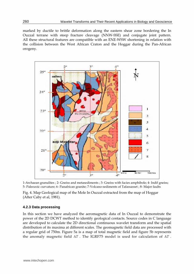
marked by ductile to brittle deformation along the eastern shear zone bordering the In Ouzzal terrane with steep fracture cleavage (NNW-SSE) and conjugate joint pattern. All these structural features are compatible with an ENE-WSW shortening in relation with the collision between the West African Craton and the Hoggar during the Pan-African orogeny.

1-Archaean granulites ; 2- Gneiss and metasediments ; 3- Gneiss with facies amphibole; 4- Indif gneiss; 5- Paleozoic curvature; 6- Panafrican granite; 7-Volcano-sediments of Tafassasset ; 8- Major faults

Fig. 4. Map Geological map of the Mole In Ouzzal extracted from the map of Hoggar (After Caby et al, 1981).

4.2.3 Data processing

In this section we have analyzed the aeromagnetic data of In Ouzzal to demonstrate the power of the 2D DCWT method to identify geological contacts. Source codes in C language are developed to calculate the 2D directional continuous wavelet transform and the spatial distribution of its maxima at different scales. The geomagnetic field data are processed with a regular grid of 750m. Figure 5a is a map of total magnetic field and figure 5b represents

the anomaly magnetic field T . The IGRF75 model is used for calculation of T .

www.intechopen.com


261

400000 440000 480000 520000 560000 600000

2420000

2440000

2460000

2480000

2500000

2520000

2540000

2560000

2580000

3335033400334503350033550336003365033700337503380033850339003395034000340503410034150342003425034300343503440034450345003455034600

X(m)

Y(m)

Fig. 5a. Total magnetic field of In Ouzzal

400000 440000 480000 520000 560000 6000002400000

2420000

2440000

2460000

2480000

2500000

2520000

2540000

2560000

2580000

-800

-600

-400

-200

0

200

400

600

800

1000

1200

X(m)

Y(m)

Fig. 5b. Anomaly magnetic field of In Ouzzal.

www.intechopen.com


262

400000 440000 480000 520000 560000 600000

2420000

2440000

2460000

2480000

2500000

2520000

2540000

2560000

2580000

-800-600-400-20002004006008001000120014001600

X(m)

Y(m)

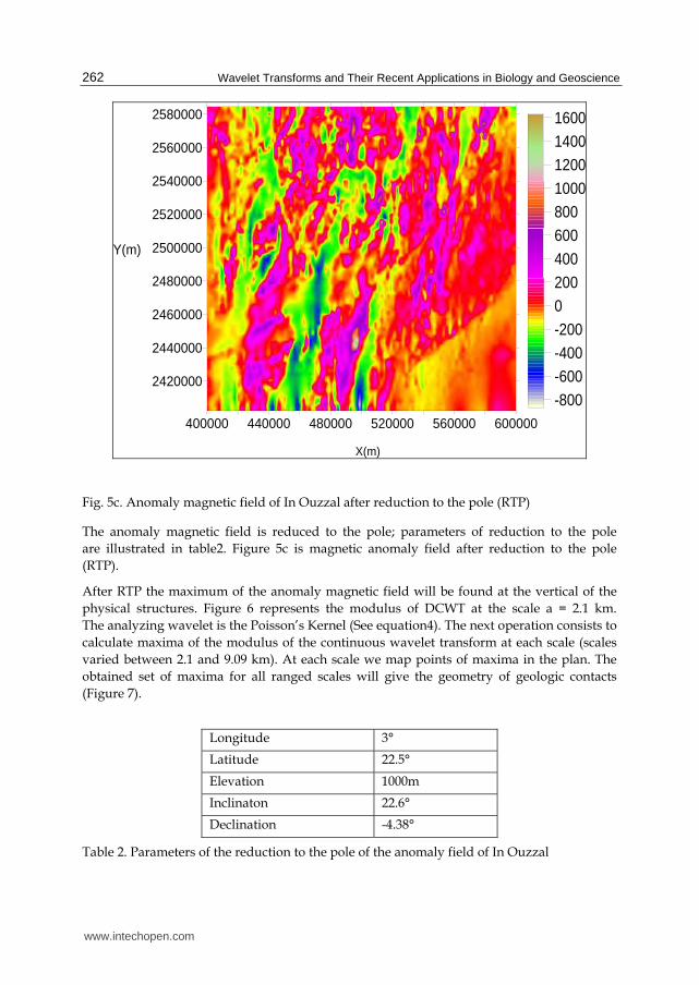
Fig. 5c. Anomaly magnetic field of In Ouzzal after reduction to the pole (RTP)

The anomaly magnetic field is reduced to the pole; parameters of reduction to the pole

are illustrated in table2. Figure 5c is magnetic anomaly field after reduction to the pole

(RTP).

After RTP the maximum of the anomaly magnetic field will be found at the vertical of the

physical structures. Figure 6 represents the modulus of DCWT at the scale a = 2.1 km.

The analyzing wavelet is the Poisson’s Kernel (See equation4). The next operation consists to

calculate maxima of the modulus of the continuous wavelet transform at each scale (scales

varied between 2.1 and 9.09 km). At each scale we map points of maxima in the plan. The

obtained set of maxima for all ranged scales will give the geometry of geologic contacts

(Figure 7).

Longitude 3°

Latitude 22.5°

Elevation 1000m

Inclinaton 22.6°

Declination -4.38°

Table 2. Parameters of the reduction to the pole of the anomaly field of In Ouzzal

www.intechopen.com


263

400000 440000 480000 520000 560000 600000

2420000

2440000

2460000

2480000

2500000

2520000

2540000

2560000

2580000

5001000150020002500300035004000450050005500600065007000750080008500900095001000010500110001150012000

X(m)

Y(m)

Fig. 6. Modulus of the 2D DCWT of the Anomaly magnetic field reduced to the pole

400000 440000 480000 520000 560000 600000

2420000

2440000

2460000

2480000

2500000

2520000

2540000

2560000

2580000

a=2121ma=2611ma=3215ma=3958ma=4873ma=6000ma=7386ma=9094mY

(m)

X(m)

Fig. 7. Mapped maxima of the 2D DCWT for all range of scales

www.intechopen.com


264

4.2.4 Results interpretation

The obtained contacts by DCWT are compared with the geological map (Figure 8). One can remark that the proposed technique is able to identify contacts that exist in the structural geology map.

Fig. 8. Obtained contacts compared with the structural map of In Ouzzal.

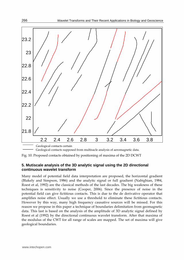
To better ensure our results, we have compared these contacts with the analytic signal (AS) solutions. The analytic signal is very sensitive to noise. This is due to the derivative operator which amplifies noise intensity (Cooper, 2006). For that we use a threshold to eliminate fictitious solutions, in this case the threshold is equal to 0.5nT/km. Figure 9 shows the comparison between contacts identified by the two methods. We can note that the AS is note able to identify a contact that exist firstly in the geological map, where 2D DCWT has identified this last (blue dashed line in figure 9). It is clear that DCWT technique has detected some contacts that not exist in the model proposed by AS (See figure 9).This is due firstly at the difference between the principles of the two techniques. In the AS technique the value of the anomaly field at the level Z=Z0 is obtained by the Hilbert transform (Nabighian, 1984). However in the proposed technique the intensity of anomaly field at Z=Z0 is defined by the modulus of 2D DCWT at the scale a=Z0. The DCWT using the Poisson Kernel is a low pass filter which decrease the noise compared to the AS technique, this last amplify the noise intensity. Figure 10 is the proposed structural model based on the mapped contacts using the 2D DCWT.

4.3 Conclusion

We have proposed a technique of boundaries identification based on the 2D directional continuous wavelet transform. Firstly we have applied this idea at a synthetic model,

www.intechopen.com


265

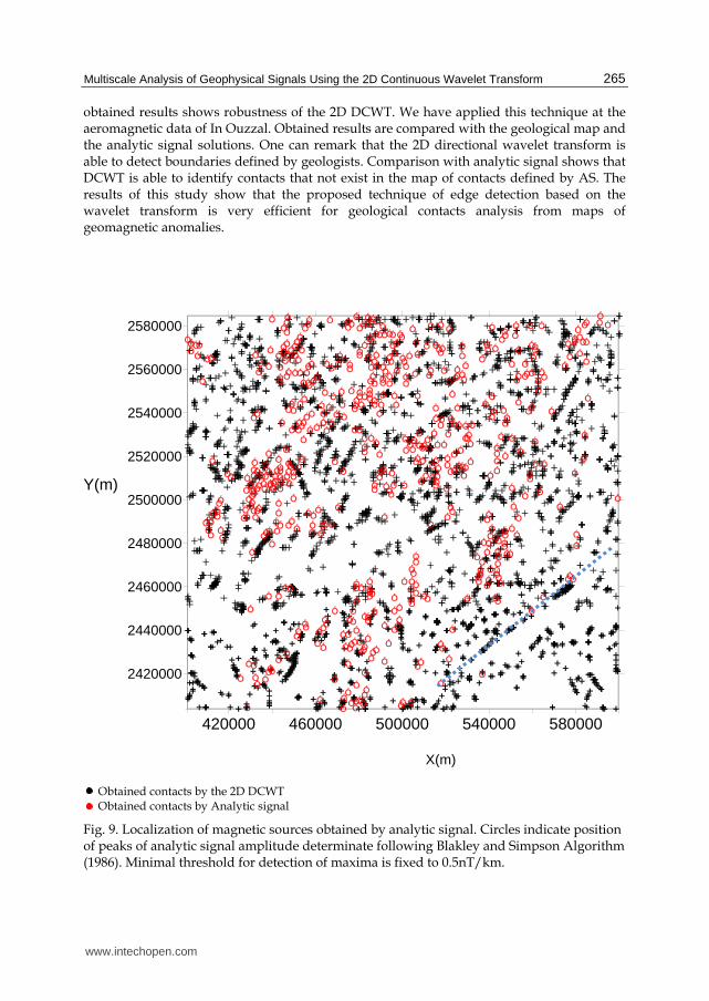
obtained results shows robustness of the 2D DCWT. We have applied this technique at the aeromagnetic data of In Ouzzal. Obtained results are compared with the geological map and the analytic signal solutions. One can remark that the 2D directional wavelet transform is able to detect boundaries defined by geologists. Comparison with analytic signal shows that DCWT is able to identify contacts that not exist in the map of contacts defined by AS. The results of this study show that the proposed technique of edge detection based on the wavelet transform is very efficient for geological contacts analysis from maps of geomagnetic anomalies.

420000 460000 500000 540000 580000

2420000

2440000

2460000

2480000

2500000

2520000

2540000

2560000

2580000

X(m)

Y(m)

Obtained contacts by the 2D DCWT Obtained contacts by Analytic signal

Fig. 9. Localization of magnetic sources obtained by analytic signal. Circles indicate position of peaks of analytic signal amplitude determinate following Blakley and Simpson Algorithm (1986). Minimal threshold for detection of maxima is fixed to 0.5nT/km.

www.intechopen.com


266

2.2 2.4 2.6 2.8 3 3.2 3.4 3.6 3.8

21.8

22

22.2

22.4

22.6

22.8

23

23.2

Geological contacts certain Geological contacts supposed from multisacle analysis of aeromagnetic data.

Fig. 10. Proposed contacts obtained by positioning of maxima of the 2D DCWT

5. Mutiscale analysis of the 3D analytic signal using the 2D directional continuous wavelet transform

Many model of potential field data interpretation are proposed, the horizontal gradient

(Blakely and Simpson, 1986) and the analytic signal or full gradient (Nabighian, 1984,

Roest et al, 1992) are the classical methods of the last decades. The big weakness of these

techniques is sensitivity to noise (Cooper, 2006). Since the presence of noise in the

potential field can give fictitious contacts. This is due to the de derivative operator that

amplifies noise effect. Usually we use a threshold to eliminate these fictitious contacts.

However by this way, many high frequency causative sources will be missed. For this

reason we propose in this paper a technique of boundaries delimitation from geomagnetic

data. This last is based on the analysis of the amplitude of 3D analytic signal defined by

Roest et al (1992) by the directional continuous wavelet transform. After that maxima of

the modulus of the CWT for all range of scales are mapped. The set of maxima will give

geological boundaries.

www.intechopen.com


267

The proposed idea has been applied on the In Ouzzal area

5.1 Analytic signal

Nabighian (1972, 1984) developed the notion of 2-D analytic signal, or energy envelope, of magnetic anomalies. Roest, et al (1992), showed that the amplitude (absolute value) of the 3-D analytic signal at location (x,y) can be easily derived from the three orthogonal gradients of the total magnetic field using the expression:

22 2

( )T T T

A xx y z

(5)

Where : ( )A x is the amplitude of the analytic signal at (x,y). T is the is the intensity of the observed magnetic field at (x,y).

An important comment at this point is the analytic signal can be easily calculated. The x and y derivatives can be calculated directly form a total magnetic field grid using a simple 3x3 filter, and the vertical gradient is routinely calculated using FFT techniques. The analytic signal anomaly over a 2-D magnetic contact located at (x=0) and at depth h is described by the expression (after Nabighian, 1972):

2 2 0.5

1( )

( )A x

h x (6)

Where is the amplitude factor 2 22 sin( )(1 cos( ) sin( ) ))M d I A h is the depth to the top of the contact. M is the strength of magnetization d is the dip of the contact I is the inclination of the magnetization vector A is the direction of the magnetization vector

5.2 The processing algorithm

The proposed idea is based on the calculation of maxima of the modulus of the 2D continuous wavelet transform of the amplitude of the analytic signal. Figure 11 shows a detailed flow chart of this technique.

Fig. 11. Flow chart of the potential field analysis using the 3D AS and 2D CWT

Calculation of amplitude of the 3D analytic signal (AS) of the potential field F

Calculation of the modulus of the continuous wavelet transform (CWT) of the amplitude of the analytic signal

Calculation of maxima of the modulus of the CWT of the AS for all range of scales

Mapping maxima of the modulus of the CWT

www.intechopen.com


268

5.3 Data processing

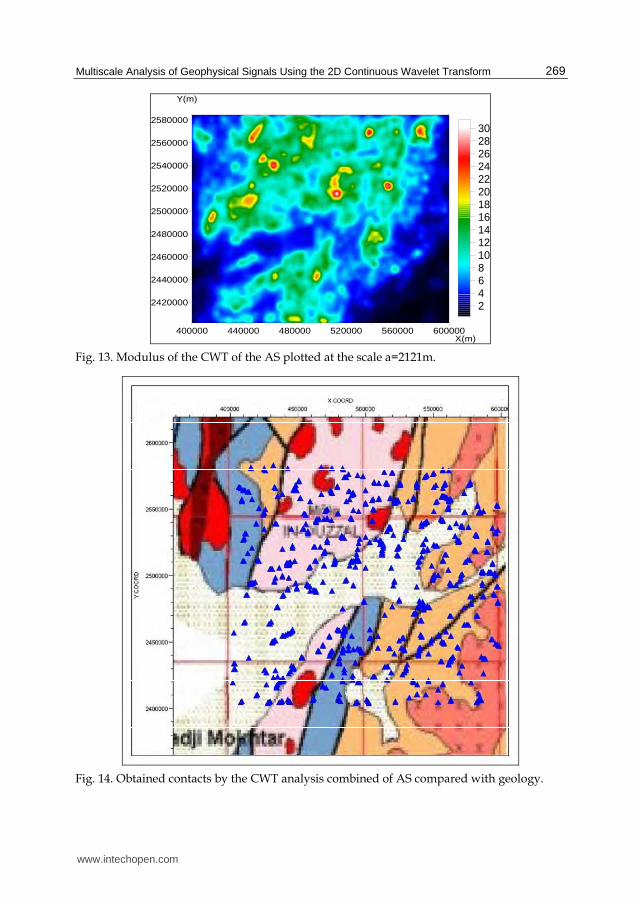
The proposed technique has been applied at the anomaly magnetic field without reduction to the pole( figure5b). The first operation consists to calculate the amplitude of the analytic signal of this field. This last is represented in figure 12. The modulus of the continuous wavelet transform of the amplitude of the AS is represented in figure 13; the analyzing wavelet is the Poisson’s Kernel. Maxima of the modulus of the CWT are mapped for all range of scales (scales varied from 2121m to 9094m). The set of maxima will give structural boundaries.

5.4 Results interpretation

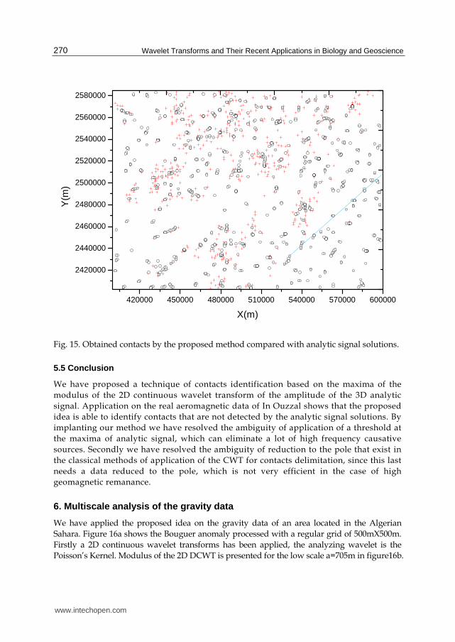
Geological contacts obtained by mapping maxima of the CWT of the amplitude the the AS are compared with geological map (See figure 14). One can remark that the proposed method is able to identify contacts defined by geology. Obtained boundaries by the proposed method are compared with contacts of analytic signal(see figure 15); for this last we have eliminated fictitious contacts dues to noise using a threshold of 0.5nT/m. We observe that by using this threshold we have eliminated a lot of contacts, for example the contact defined by the dashed line in figure 15 is identified by the CWT combined with AS, however it is not detected by analytic signal, this is due to the threshold effect, this last has been applied to reduce the noise effect on the AS.

400000 440000 480000 520000 560000 600000

2420000

2440000

2460000

2480000

2500000

2520000

2540000

2560000

2580000

0.10.20.30.40.50.60.70.80.911.11.21.31.41.51.6

X(m)

Y(m)

Fig. 12. Amplitude of the analytic signal of the anomaly magnetic field of In-Ouzzal

www.intechopen.com


269

400000 440000 480000 520000 560000 600000

2420000

2440000

2460000

2480000

2500000

2520000

2540000

2560000

2580000

24681012141618202224262830

X(m)

Y(m)

Fig. 13. Modulus of the CWT of the AS plotted at the scale a=2121m.

Fig. 14. Obtained contacts by the CWT analysis combined of AS compared with geology.

www.intechopen.com


270

420000 450000 480000 510000 540000 570000 600000

2420000

2440000

2460000

2480000

2500000

2520000

2540000

2560000

2580000

Y(m

)

X(m)

Fig. 15. Obtained contacts by the proposed method compared with analytic signal solutions.

5.5 Conclusion

We have proposed a technique of contacts identification based on the maxima of the

modulus of the 2D continuous wavelet transform of the amplitude of the 3D analytic

signal. Application on the real aeromagnetic data of In Ouzzal shows that the proposed

idea is able to identify contacts that are not detected by the analytic signal solutions. By

implanting our method we have resolved the ambiguity of application of a threshold at

the maxima of analytic signal, which can eliminate a lot of high frequency causative

sources. Secondly we have resolved the ambiguity of reduction to the pole that exist in

the classical methods of application of the CWT for contacts delimitation, since this last

needs a data reduced to the pole, which is not very efficient in the case of high

geomagnetic remanance.

6. Multiscale analysis of the gravity data

We have applied the proposed idea on the gravity data of an area located in the Algerian

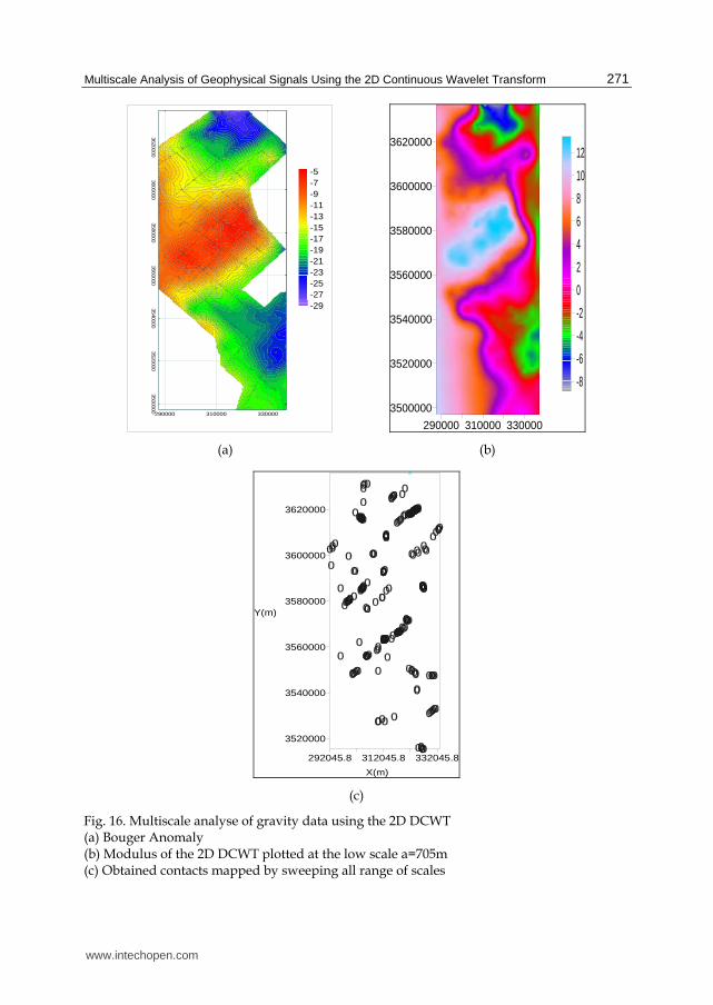
Sahara. Figure 16a shows the Bouguer anomaly processed with a regular grid of 500mX500m.

Firstly a 2D continuous wavelet transforms has been applied, the analyzing wavelet is the

Poisson’s Kernel. Modulus of the 2D DCWT is presented for the low scale a=705m in figure16b.

www.intechopen.com


271

290000 310000 330000

35000003520000

35400003560000

35800003600000

3620000

-29-27-25-23-21-19-17-15-13-11-9-7-5

290000 310000 330000

3500000

3520000

3540000

3560000

3580000

3600000

3620000

-8

-6

-4

-2

0

2

4

6

8

10

12

(a) (b)

292045.8 312045.8 332045.8

3520000

3540000

3560000

3580000

3600000

3620000

X(m)

Y(m)

(c)

Fig. 16. Multiscale analyse of gravity data using the 2D DCWT (a) Bouger Anomaly (b) Modulus of the 2D DCWT plotted at the low scale a=705m (c) Obtained contacts mapped by sweeping all range of scales

www.intechopen.com


272

The maxima of the modulus of the continuous wavelet transform have been mapped for all range of scales. Figure 16c shows the map of the obtained boundaries, obtained results are compared with a seismic profile that passes by the prospected region, it exhibits a big correlation.

7. Multiscale analysis of noisy 3D GPR data

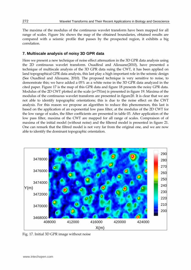
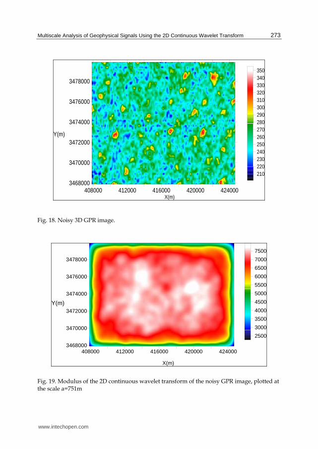
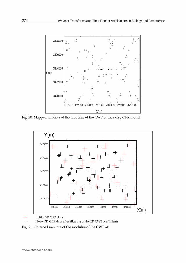
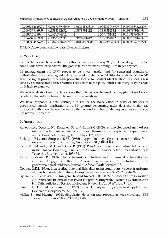
Here we present a new technique of noise effect attenuation in the 3D GPR data analysis using the 2D continuous wavelet transform. Ouadfeul and Aliouane(2010), have presented a technique of multiscale analysis of the 3D GPR data suing the CWT, it has been applied on land topographical GPR data analysis, this last play a high important role in the seismic design (See Ouadfeul and Aliouane, 2010). The proposed technique is very sensitive to noise, to demonstrate this; we have added a 05% as a white noise in the 3D GPR data analyzed in the cited paper. Figure 17 is the map of this GPR data and figure 18 presents the noisy GPR data. Modulus of the 2D CWT plotted at the scale (a=751m) is presented in figure 19. Maxima of the modulus of the continuous wavelet transform are presented in figure20. It is clear that we are not able to identify topographic orientations; this is due to the noise effect on the CWT analysis. For this reason we propose an algorithm to reduce this phenomenon, this last is based on the application of an exponential low pass filter, at the modulus of the 2D CWT for the low range of scales, the filter coefficients are presented in table 03. After application of the low pass filter, maxima of the CWT are mapped for all range of scales. Compraison of of maxima of the initial model (without noise) and the filtered model is presented in figure 21. One can remark that the filtred model is not very far from the original one, and we are now able to identify the dominant topographic orientation.

408000 412000 416000 420000 4240003468000

3470000

3472000

3474000

3476000

3478000

200

210

220

230

240

250

260

270

280

290

X(m)

Y(m)

Fig. 17. Initial 3D GPR image without noise

www.intechopen.com


273

408000 412000 416000 420000 4240003468000

3470000

3472000

3474000

3476000

3478000

210220230240250260270280290300310320330340350

X(m)

Y(m)

Fig. 18. Noisy 3D GPR image.

408000 412000 416000 420000 4240003468000

3470000

3472000

3474000

3476000

3478000

2500

3000

3500

4000

4500

5000

5500

6000

6500

7000

7500

X(m)

Y(m)

Fig. 19. Modulus of the 2D continuous wavelet transform of the noisy GPR image, plotted at the scale a=751m

www.intechopen.com


274

410000 412000 414000 416000 418000 420000 422000

3470000

3472000

3474000

3476000

3478000

X(m)

Y(m)

Fig. 20. Mapped maxima of the modulus of the CWT of the noisy GPR model

410000 412000 414000 416000 418000 420000 422000

3470000

3472000

3474000

3476000

3478000

X(m)

Y(m)

Initial 3D GPR data Noisy 3D GPR data after filtering of the 2D CWT coefficients

Fig. 21. Obtained maxima of the modulus of the CWT of:

www.intechopen.com


275

0.0003354626279 0.006737946999 0.01831563889 0.006737946999 0.0003354626279 0.006737946999 0.1353352832 0.3678794412 0.1353352832 0.006737946999 0.01831563889 0.3678794412 1 0.3678794412 0.01831563889 0.006737946999 0.1353352832 0.3678794412 0.1353352832 0.006737946999 0.0003354626279 0.006737946999 0.01831563889 0.006737946999 0.0003354626279

Table 3. An exponential low pass filter coefficients

8. Conclusion

In this chapter we have realize a multiscale analysis of many 2D geophysical signals by the continuous wavelet transform, the goal is to resolve many ambiguities in geophysics.

In geomagnetism the CWT proves to be a very useful tool for structural boundaries delimitation from geomagnetic data reduced to the pole. Multiscale analysis of the 3D analytic signal proves to be very powerful tool to for contact identification, this tool is less sensitive to noise and doesn’t require a reduction to the pole, which is not very easy in areas with high remanance.

Wavelet analysis of gravity data shows that this last can be used for mapping of geological accidents, this information can be used for seismic design.

We have proposed a new technique to reduce the noise effect in wavelet analysis of geophysical signals, application on a 3D ground penetrating radar data shows that the proposed method can be used to reduce the noise effect when analyzing geophysical data by the wavelet transform.

9. References

Arneodo,A., Decoster,N., Kestener, P., and Roux,S.G.(2003). A wavelet-based method for multi- fractal image analysis: From theoretical concepts to experimental applications. Adv. Imaging Electr. Phys. 126, 1-92.

Blakely , R.J., and Simpson, R.W. (1986). Approximating edges of source bodies from magnetic or gravity anomalies, Geophysics : 51 ,1494–1498.

Caby. R, Bertrand. J. M. L, and Black. R. (1981). Pan-African closure and ontinental collision in the Hoggar-Iforas segment, central Sahara. in Kroner A (ed) Precambrian Plate Tectonics, Elsevier, Amst. 407-434.

Caby. R, Monie. P. (2003). Neoproterozoic subduction and differential exhumation of western Hoggar (southwest Algeria): new sructural, petrological and geochronological evidence, Journal of African Earth Sciences. 37.

Cooper, G.R.J. (2006). Interpreting potential field data using continuous wavelet transforms of their horizontal derivatives, Computers & Geosciences 32 (2006) 984–992

Djemaï, S., , Haddoum, H., Ouzegane. K, And Kienast, J-R. (2009). Archaean Series Reworked At Proterozoic In Amesmessa (West Hoggar): Cartography, Tectonic Evolution And P-T Path, Bulletin du Service Géologique National, Vol. 20, n°1, pp. 3 – 29.

Kumar, P., Foufoula-Georgiou, E. (1997). wavelet analysis for geophysical applications, Reviews of Geophysics,35,4, 385-412.

Mallat, S., and Hwang. (1992). Singularity detection and processing with wavelets, IEEE Trans. Info. Theory 38(2), 617-643, 1992.

www.intechopen.com


276

Martelet, G., Sailhac, P., Moreau, F., Diament, M.(2001). Characterization of geological boundaries using 1-D wavelet transform on gravity data: theory and application to the Himalayas. Geophysics 66, 1116–1129.

Moreau, F., D. Gibert, M. Holschneider, and G. Saracco. (1999). Identification of sources of potential fields with the continuous wavelet transform: Basic theory, J. Geophys. Res., 104, 5003–5013.

Moreau , F., Gibert, D., Holschneider M., Saracco G. (1997). Wavelet analysis of potential fields. Inverse Problem, 13, 165-178.

Murenzi, R., 1989, Transformée en ondelettes multidimensionnelle et application à l’analyse d’images, Thèse Louvain-La-Neuve.

Nabighian, M. N. 1(972). The analytic signal of two-dimensional magnetic bodies with polygonal cross-section: Its properties and use of automated anomaly interpretation: Geophysics, 37, 507–517, doi: 10.1190/1.1440276.

Nabighian, M.N. (1984). Toward a three-dimensional automatic interpretation of potential field data via generalized Hilbert transforms: Fundamental relations: Geophysics, 49 ,957–966.

Ouzegane K, Boumaza. S. (1996). An example of ultra-high temperature metamorphism : orthpyroxene-sillimnite, -garnet, sapphirine-quartz and spinel-quartz parageneses in Al-Mg granulites froum In Hihaou, In Ouzzal, Hoggar, Journal of Metamorphic Geology, 14: 693-708.

Ouadfeul , S. (2006). Automatic lithofacies segmentation using the wavelet transform modulus maxima lines (WTMM) combined with the detrended fluctuation analysis (DFA), 17the International geophysical congress and exhibition of turkey, Expanded abstract .

Ouadfeul , S. ( 2007). Very fines layers delimitation using the wavelet transform modulus maxima lines WTMM combined with the DWT , SEG SRW , Expanded abstract.

Ouadfeul, S.(2008). Reservoir characterization using the continuous wavelet transform combined with the Self Organizing map (SOM) neural network: SPE ECMOR XI, Expanded abstract.

Ouadfeul, S., and Aliouane, L. (2010). Multiscale of 3D GPR data using the continuous wavelet transform, presented in GPR2010,IEEE, doi: 10.1109/ ICGPR.2010.5550177.

Ouadfeul, S, Aliouane, L., Eladj, S. (2010). Multiscale analysis of geomagnetic data using the continuous wavelet transform. Application to Hoggar (Algeria), SEG Expanded Abstracts 29, 1222 (2010); doi:10.1190/1.3513065.

Reid, A.B., Allsop, J.M., Granser, H., Millett, A.J., Somerton, I.W.(1990). Magnetic interpretation in three dimensions using Euler deconvolution: Geophysics, 55, 80–91.

Roest, W.R, Verhoef, J, and Pilkington, M. (1992). Magnetic interpretation using the 3-D signal analytic, Geophysics, 57:116-125.

Sailhac. P, Galdeano. A, Gibert. D, Moreau. F, and Delor. C. (2000). Identification of sources of potential fields with the continuous wavelet transform: Complex wavelets and applications to magnetic profiles in French Guiana, J, Geophy, Res., 105: 19455-75.

Sailhac , P., and Gibert , D. (2003). Identification of sources of potential fields with the continuous wavelet transform: Two-dimensional wavelets and multipolar approximations, Journal of geophysical research, vol. 108, noB5.

Sailhac, P., Galdeano, A., Gibert, D., Moreau, F., Delor, C. (2000). Identification of sources of potential fields with the continuous wavelet transform: complex wavelets and application to aeromagnetic profiles in French Guiana. Journal of Geophysical Research 105, 19455–19475.

Valee, M.A., Keating, P., Smith, R.S., St-Hilaire, C. (2004). Estimating depth and model type using the continuous wavelet transform of magnetic data. Geophysics 69, 191–199.

www.intechopen.com

Wavelet Transforms and Their Recent Applications in Biology andGeoscienceEdited by Dr. Dumitru Baleanu

ISBN 978-953-51-0212-0Hard cover, 298 pagesPublisher InTechPublished online 02, March, 2012Published in print edition March, 2012

InTech EuropeUniversity Campus STeP Ri Slavka Krautzeka 83/A 51000 Rijeka, Croatia Phone: +385 (51) 770 447 Fax: +385 (51) 686 166www.intechopen.com

InTech ChinaUnit 405, Office Block, Hotel Equatorial Shanghai No.65, Yan An Road (West), Shanghai, 200040, China

Phone: +86-21-62489820 Fax: +86-21-62489821

This book reports on recent applications in biology and geoscience. Among them we mention the application ofwavelet transforms in the treatment of EEG signals, the dimensionality reduction of the gait recognitionframework, the biometric identification and verification. The book also contains applications of the wavelettransforms in the analysis of data collected from sport and breast cancer. The denoting procedure is analyzedwithin wavelet transform and applied on data coming from real world applications. The book ends with twoimportant applications of the wavelet transforms in geoscience.

How to referenceIn order to correctly reference this scholarly work, feel free to copy and paste the following:

Sid-Ali Ouadfeul, Leila Aliouane, Mohamed Hamoudi, Amar Boudella and Said Eladj (2012). MultiscaleAnalysis of Geophysical Signals Using the 2D Continuous Wavelet Transform, Wavelet Transforms and TheirRecent Applications in Biology and Geoscience, Dr. Dumitru Baleanu (Ed.), ISBN: 978-953-51-0212-0, InTech,Available from: http://www.intechopen.com/books/wavelet-transforms-and-their-recent-applications-in-biology-and-geoscience/multiscale-analysis-of-geophysical-signals-using-the-2d-continuous-wavelet-transform

sid-ali ouadfeul , leila aliouane - intech -...

Documents