Sign Restrictions in Structural VectorAutoregressions: A Critical Review�

Renee Fryy and Adrian Paganz

December 1, 2009

Contents

1 Introduction 2

2 Summarizing the Data and Structural Representations 52.1 VAR and SVAR Representations . . . . . . . . . . . . . . . . 52.2 Other Representations . . . . . . . . . . . . . . . . . . . . . . 72.3 Two examples . . . . . . . . . . . . . . . . . . . . . . . . . . . 8

2.3.1 A Market (Demand/Supply) Model . . . . . . . . . . . 82.3.2 A Small Macro Model . . . . . . . . . . . . . . . . . . 9

3 Methodology And Informativeness of SVARModelling UsingSign Restrictions 103.1 Generating Candidate Shocks . . . . . . . . . . . . . . . . . . 10

3.1.1 Multiple Shocks . . . . . . . . . . . . . . . . . . . . . . 103.1.2 A Single Shock . . . . . . . . . . . . . . . . . . . . . . 123.1.3 Permanent and Transitory Shocks . . . . . . . . . . . . 133.1.4 Givens Matrices . . . . . . . . . . . . . . . . . . . . . . 133.1.5 Householder Transformations . . . . . . . . . . . . . . 15

3.2 Shock Identi�cation Issues . . . . . . . . . . . . . . . . . . . . 15�We are greatful to referees for some very helpful suggestions regarding the structure

of this review.yAustralian National UniversityzUniversity of New South Wales and Queensland University of Technology

1

3.2.1 The Parametric Approaches . . . . . . . . . . . . . . . 153.2.2 Ensuring Structural Identi�cation with Sign Restrictions 163.2.3 Model Identi�cation . . . . . . . . . . . . . . . . . . . 17

3.3 Information Provided by Sign Restrictions: Can We RecoverCorrect Impulse Responses? . . . . . . . . . . . . . . . . . . . 23

3.4 Sources of Information for Sign Restrictions . . . . . . . . . . 24

4 Sign Restrictions in Practice 264.1 Technology and Productivity . . . . . . . . . . . . . . . . . . . 274.2 Fluctuations . . . . . . . . . . . . . . . . . . . . . . . . . . . . 294.3 Monetary and Fiscal Policy . . . . . . . . . . . . . . . . . . . 324.4 Exchange Rates . . . . . . . . . . . . . . . . . . . . . . . . . . 364.5 Miscellaneous . . . . . . . . . . . . . . . . . . . . . . . . . . . 39

5 Conclusion 41

6 References 42

7 Appendix 47

1 Introduction

Structural Vector Autoregressions (SVARs) have become one of the majorways of extracting information about the macro economy. One might citethree major uses of them in macro-econometric research.1. For quantifying impulse responses to macroeconomic shocks.2. For measuring the degree of uncertainty about the impulse responses

or other quantities formed from them.3. For deciding on the contribution of di¤erent shocks to business cycles

and forecast errors through variance decompositions.To determine this information a VAR is �rst �tted to summarize the data

and then a structural VAR (SVAR) is proposed whose structural equation er-rors are taken to be the economic shocks. The parameters of these structuralequations are then estimated by utilizing the information in the VAR. TheVAR is a reduced form which summarizes the data; the SVAR provides aninterpretation of the data. As for any set of structural equations, recovery ofthe structural equation parameters (shocks) requires the use of identi�cationrestrictions that reduce the number of "free" parameters in the structural

2

equations to the number that can be recovered from the information in thereduced form.Five major methods for recovering the structural equation parameters are

listed below. The �rst four utilize parametric restrictions to produce enoughinstruments for the contemporaneous endogenous variables that appear inthe structural equations.(i) In the original approach to structural equation estimation the Cowles

Commission regarded the structural shocks as being correlated and solved theidenti�cation problem by excluding variables from the structural equations.Often the excluded variables were lagged endogenous variables. One disad-vantage of this solution is that any correlation between the shocks makesexercises involving the decomposition of the variance of a variable into thecontribution from separate structural shocks infeasible.(ii) Following Wold (1951) and Quenouille (1957), Sims (1980) proposed

that the structural system be made recursive and that no restriction beplaced upon the dynamics. Recursivity actually embodies two separate as-sumptions - that the shocks in the structural equations be uncorrelated withone another and that the endogenous variables can be arranged (ordered) sothat each contemporaneously depends on others further down the system,but not on those above i.e. the system is made to exhibit a triangular struc-ture. The triangularity might be justi�ed by institutional knowledge, whilethe plausibility of the uncorrelated shocks depends on whether the SVARadequately captures the macro-economic system. In turn this latter featurerequires both a su¢ cient number of variables to be included in the VAR anda lag length of high enough order to adequately capture the dynamics.(iii) Recognizing that some macro-economic variables are best thought of

as being stochastically non-stationary brings in the fact that there may beshocks with permanent e¤ects upon those variables. "Long-run restrictions"exploit this fact. Denoting the j0th horizon impulse responses of the variablesto the shocks as Cj; the long-run e¤ects of shocks will be C1: A permanente¤ect of the i0th shock upon the k0th variable is then distinguished from atransitory shock by there being a non-zero element in the k0th row and i0thcolumn of C1. These can be translated into linear restrictions upon thestructural coe¢ cients of an SVAR - see Shapiro and Watson (1988), Paganand Robertson (1998). Such restrictions reduce the number of parameters tobe estimated and free up instruments from among the lagged values of thevariables.(iv) Parametric impulse response restrictions are sometimes used to pro-

3

vide identi�cation. For example, if it is assumed that the i 0th structuralshock has no immediate e¤ect upon a variable ykt, this can be shown tomean that the errors in the VAR equation for ykt are not a function of thei�th structural shock - see Pagan and Robertson(1998). It follows then thatthe residuals from this equation can be used as an instrument in the struc-tural equation for ykt, provided the assumption that the structural shocksare uncorrelated is correct.All of the methods described above impose parametric restrictions. Re-

cently, a �fth method for estimating SVARs has arisen that employs signrestrictions upon the impulse responses as a way of identifying shocks. Italso assumes that shocks are uncorrelated. Applications of this method havebeen growing as seen in the papers listed in Table 3. Consequently, it isworth examining this literature in more detail and the aim of our paper is toexposit how the method works, to identify some di¢ culties in its application,and to examine the empirical work gathered in Table 3.In practical applications it is often found that a combination of all the

methods mentioned above need to be employed in order to be able to identifyall the shocks of interest. We emphasize that which of the �ve methodsnoted above is used in practice does not depend on the data, but rather onthe preferences of the investigator and/or of those who wish to utilize anSVAR to study some issue. These preferences may well be incompatible assome users may feel that certain types of restrictions are more plausible thanothers. Prima facie it does seem likely that long-run and sign restrictionswould be regarded as less restrictive than the other approaches, but without aspeci�c context we have no basis for recommending any particular approach.Each has di¢ culties and these need to be understood to make an informedjudgement on their utility. Although it is likely in practice that a mixed setof restrictions will be employed, because the literature on sign restrictionsis more recent than that on the other methods it is convenient to simplyassume that only sign restrictions are being employed.Section 2 asks how the data should be summarized? The existing lit-

erature implicitly assumes that the answer is a VAR in some observablevariables. But this may not be satisfactory in all contexts. First, when thereare permanent shocks and co-integration between variables a VECM ratherthan a VAR will be needed. Second, if we wish to align the summary modelwith theoretical models it is often necessary to recognize that, whilst thelatter generally implies a VAR in all the model variables, in practice onlya sub-set often appear in the VAR that is estimated on actual data. This

4

discrepancy may either be because some of the model variables are latent orbecause they are believed to be hard to measure accurately. When there is adivergence it becomes important to ask whether a VAR is the right vehicleto adopt as the summative model, and how one would proceed to apply signrestrictions if the context suggests that it is not. This section also introducestwo simple models that are useful for understanding the issues raised in theapplication of sign restrictions - a two equation market model ( supply anddemand) and a three equation macro model.Section 3 begins by setting out the techniques that have been proposed

to apply sign restrictions and brie�y describes the main numerical meth-ods used. It then looks at how each of the parametric and sign-restrictionapproaches works in the context of the market model. In all approaches,parametric or sign-restricted, the restrictions are designed to solve what willbe called the structural identi�cation problem. However they leave unresolvedwhat Preston (1978) called the model identi�cation problem. The problemseems to have elicited much more attention in the sign restrictions literatureand so we look at the various suggestions that have been made about howto handle it. Finally, we close the section by looking at what can be learnedfrom the use of sign restrictions and where the restrictions might come from.To answer the latter we utilize the New Keynesian model as a prototype forhow some suggestions have been made about isolating suitable sign informa-tion. Section 4 surveys some existing empirical applications and provides anaccount of how they have proceeded, where the sign information came from,and what di¢ culties arise in the way the authors have proceeded. It is ourcontention that one needs a template for examining such studies and we seekto provide that. Section 5 concludes.

2 Summarizing the Data and Structural Rep-resentations

2.1 VAR and SVAR Representations

Most of the literature we deal with assumes that the data is represented bya VAR ( for simplicity we will make it �rst order)

zt = A1zt�1 + et;

5

where zt is an n � 1 vector of variables. From this an interpretation of thedata is provided through a SVAR

B0zt = B1zt�1 + "t;

which implies that B0et = "t i.e. the structural shocks we seek to measureare linear combinations of the VAR errors et: The latter can be estimated bythe VAR residuals et: To estimate the structural (economic) shocks, "t; thenrequires that one construct an appropriate set of weights (B0) on et: Clearlythe VAR is the reduced form of the structure set out in the SVAR.The solution to the VAR(1) is the MA form

zt = D0et +D1et�1 +D2et�2 + :::

where Dj is the j�th period impulse response of zt+j to a unit change in et(D0 = In): It follows that the MA form for the SVAR is

zt = C0"t + C1"t�1:::;

with the impulse responses to "t being Cj = DjB�10 = DjC0:

The VAR is easily estimated by OLS regardless of the nature of theSVAR. Hence Dj can always be estimated once the lag length of the VAR isspeci�ed. Because Cj = DjC0; and Dj is �xed by the data independently ofany structural model, all restrictions that are placed on Cj are e¤ectively justrestrictions upon combinations of the columns of C0; with the weights usedin forming such combinations being the rows of Dj. To understand manyissues regarding sign restrictions it is important to realize that we are alwaysrestricting the elements of C0: Such restrictions might be imposed on C0directly but they also derive from restrictions on impulses at longer horizonse.g. information about the signs of the elements of C1 imply constraints uponcombinations of the elements of C0: If the restrictions on C1 are quantitativethis fact narrows the possible values of C0: However, the same e¤ect does notnecessarily hold for sign restrictions. For example, if all elements of C0 arepositive, and so too are the estimated D1 from the data, then a restrictionthat the elements of C1 are positive adds nothing to what has already beenassumed about the signs of C0: There is a belief in the literature that addingon sign restrictions for longer impulse responses, Cj; j > 0; provides strongeridentifying information. This seems to stem from the Monte Carlo work inPaustian (2007). It is clear from the connections that exist between the Cjand C0 noted above that nothing guarantees this.

6

2.2 Other Representations

Now if we try to align theory-inspired interpretative models ( such as DSGEmodels) with the summative model we often encounter the situation thatthere are variables in the former that are not observable and so the lattermodel is �tted with a smaller number of variables.1 Let the observable vari-ables (data) be zt and the larger set in the theoretical model be z+t : Then,it has been known for a long time, see Wallis(1977) and Zellner and Palm(1974), that a VAR in z+t becomes a VARMA in zt: Thus a VAR will notrepresent the data precisely if it should be generated by a theoretical modelwith latent (unobserved) variables, although if one makes the order su¢ -ciently high it might be argued to be approximately correct. Basically thisimplies that the impulse responses from the theoretical model, C+j ; will notbe equal to those from an approximating VAR, unless the order is in�nite.As shown in Kapetanios et al (2006), this di¤erence can be very large forsome shocks and models and so one needs to exercise care in using informa-tion from theory-consistent models to identify shocks in VARs.2 Of course itis possible that this problem is less of an issue for the signs of the responsesthan it is for the magnitudes i.e. the signs of C+j and Cj may agree even ifthe magnitudes don�t. Fundamentally the problem is that a VAR is not thecorrect summative model.3 As an alternative one might estimate a VARMAprocess or a VAR with some latent variables but it is probably simpler tofocus on the state space form

zt = Hz+tz+t = Mz+t�1 + e+t

and estimate this. Readily available computer programs such as Dynare aredesigned to do so. Thus the role of a theory-inspired model is to provide thevariables in z+t and the order of the VAR associated with them, while theempirical investigator selects zt. Because sign restrictions often come fromDSGE models we return to the issue later.

1Technology is an obvious example of a variable in a DSGE model that is rarely presentin an estimated VAR. But it is also the case that researchers often treat the capital stockas unobservable and so it is omitted from the list of variables in the empirical VAR.

2Using a model that was a smaller version of BEQM and a VAR with a standard set ofsix variables it was found that a VAR(50) and thirty thousand observations were neededto recover the true impulse responses.

3There are even cases where there is no invertible MA representation, and so no VARexists.

7

If there are permanent shocks with no co-integration between variablesthen the VAR and SVAR will simply involve di¤erences in the variables ztrather than the levels, so it is just how the data is measured that changes.Sometimes one sees the summative model in the sign restrictions literatureas a DVAR i.e. a VAR in the di¤erences �zt: Examples are Jarocinski andSmets (2008) and Farrant and Peersman (2006). Often it does not seem tobe appreciated that in this case all shocks are permanent ( assuming that theonly variables in zt are I(1)): When there is co-integration the summativemodel will be the Vector Error Correction Model (VECM)

�z+t = ��0z+t�1 + et;

and a Structural VECM (SVECM) will interpret this data

B0�z+t = (B0�)�

0z+t�1 + "t: (1)

Thus, as these are relatively simple extensions of the standard approach, onedoes not need any special development. It should be emphasized that theVECM would be in z+t rather than (observed) zt; as the level of the log oftechnology will generally be a latent variable appearing in z+t but not in zt:Thus the problems identi�ed above relating to latent variables occur againalthough they can be solved in the same way viz. via the state space form.

2.3 Two examples

2.3.1 A Market (Demand/Supply) Model

We take the case of a simple model comprising a demand and a supplyfunction with associated shocks. Speci�cally the SVAR system will be

qt = ��pt + �qqqt�1 + �qppt�1 + "Dt (2)

pt = qt + �pqqt�1 + �pppt�1 + "St; (3)

Hence in terms of the SVAR discussion above zt =�qtpt

�: The reduced form

of the market model is a VAR(1). Since the equations (2) and (3) are essen-tially identical for arbitrary parameter values, at this point there is nothingwhich distinguishes the demand ("Dt) and supply shocks ("St); and the taskis to introduce extra information that does enable us to identify these. It

8

would seem likely that most researchers would agree with the sign informa-tion in Table 1 for the impact of positive shocks upon the contemporaneousvariables. Since the patterns are distinct this suggests that we can identifyseparate shocks.There is one complication. Because a negative movement in each shock

would produce a pattern in C0 of�� +� �

�it is necessary to recognize that

such a sign pattern is also consistent with demand and supply shocks, albeit

negative ones. This is clearly not the end of the matter, since�� �� +

�and

�+ ++ �

�are also indicative of demand and supply shocks, but now of

opposite signs. So one needs to allow for all of these possibilities in deciding ifa given pattern in impulse responses is consistent with a demand and supplyshock. Clearly the need to check for the complete set of compatible signrestrictions will grow as the number of shocks increases.

Table 1: Sign Restrictions for MarketModel (Demand/Supply) Shocks

variablenshock Demand Supplypt + -qt + +

2.3.2 A Small Macro Model

A small macro model that is used a lot involves an output gap (yt); in�ation(�t) and a policy interest rate (it): i.e. z0t =

�yt �t it

�: A typical SVAR

model for these variables would be

yt = z0t�1 y + �yiit + �y��t + "yt (4)

�t = z0t�1 � + ��iit + ��yyt + "�t (5)

it = z0t�1 i + �iyyt + �i��t + "it (6)

The three shocks will be monetary policy ("it), a demand shock ("yt) and acost-push ( supply) shock ("�t). For simplicity the shocks will be treated ashaving no serial correlation, so that the reduced form is a VAR(1). The signsof the contemporaneous e¤ects to positive shocks will most likely be those

9

in Table 2. Again these are distinct and so should enable the separation ofthe three structural shocks. Again we would need to recognize the problemwith di¤erent signs, as there will now be nine possible signs for the C0 thatare compatible with the presence of the three postulated shocks.

Table 2: Sign Restrictions for Macro Model Shocks

variablenshock Demand Cost-Push Interest Rateyt + - -�t + + -it + + +

3 Methodology And Informativeness of SVARModelling Using Sign Restrictions

3.1 Generating Candidate Shocks

3.1.1 Multiple Shocks

In all cases a set of n estimated shocks et will be available from the model wechoose to be the summative one. By combining them in an appropriate waywe can produce candidate structural shocks "t that are uncorrelated. Nowthere will be many such combinations. Some of them will produce impulseresponses that have the correct signs while others won�t. Thus in the marketmodel case there will only be some weights which produce shocks that respectthe patterns in Table 1. So our �rst task is to select an algorithm that givesa set of weights: Once one has these we can check if they are "successful",in that the impulse response functions Cj for the corresponding structuralshocks agree with the postulated sign information. If they are not successfulwe will discard them and "draw" another set of weights.Now the critical constraint needed in designing an algorithm to do this is

that the generated weights must be such as to ensure that the constructedstructural shocks "t are uncorrelated. Suppose we begin by �rst estimating arecursive VAR. In that case after estimation we would have et = B�1

0 "t; whereB0 is triangular. By design these structural shocks, "t; are uncorrelated.However, rather than work with these it is often more useful to work withshocks that have unit variance, and this can be done by dividing each ofthe "kt by its standard deviation. Hence, let S be the matrix that has the

10

estimated standard deviations of the "t on the diagonal and zeros elsewhere.Then et = B�1

0 SS�1"t = T �t; where �t = S�1"t are now new structuralshocks that do possess unit variances. These �t shocks will be termed ourbase set. Notice that they are just a re-scaled version of the "t; so their naturehas not changed.4

Now we form combinations of the �t using a matrix Q i.e. ��t = Q�t: The

��t are candidates for "named" structural shocks e.g. "supply" and "demand".They need to be uncorrelated and so Q must be restricted: The appropriaterestriction is that Q is a square matrix such that Q0Q = QQ0 = In; sincethat means

et = TQ0Q�t= T ���t ;

and cov(��t��0t ) = Qcov(�

t�0t)Q0 = In: Thus we have found a new set of shocks,

��t ; that have the same covariance matrix as �t (and which will reproduce thevar(zt)); but which will have a di¤erent impact (T �) upon et and, hence, thevariables zt i.e. produce di¤erent impulse responses: It is this ability to createa large number of candidate shocks with varying impulse responses that isthe basis of sign restriction methods. It is clearly very simple to constructall these shocks using programs that do matrix operations once we have amethod for forming a Q that has the property Q0Q = QQ0 = In: There aremany such Q0s and we will refer to each as a "draw".How does one �nd a Q matrix? There are actually quite a few ways

of doing this. The two most popular utilize Givens and Householder trans-formations (the latter is the basis of the Q-R decomposition used in manyill-conditioned regression problems), but this does not exhaust the possibil-ities. We provide an account of each of these and the relationship betweenthem in later sub-sections.

4Numerically it is generally more e¢ cient to estimate �t by estimating the covariancematrix of the residuals et; ; and then applying a Cholesky decomposition T�1T 0�1 = Into get T : Then �t = T�1et: This is a useful way of proceeding since all that is neededto implement it is the estimated covariance matrix of the errors in the equations of thesummative model. It also means that the summative model need not be a VAR. It couldbe a VECM or a state space model.

11

3.1.2 A Single Shock

In the description above it was assumed that n shocks were to be found.But sometimes only a single shock is of interest. To �nd this we might stillutilize the n � n Q-matrices above. In doing so we would be producing nuncorrelated structural shocks, but only choosing to focus upon one of them.Two issues arise here. Firstly, in some papers one has the impression that itis only necessary that the weights used for constructing the structural shocksbe an n�1 vector q that has unit length. Uhlig�s papers often state it in thisway e.g Scholl and Uhlig (2008, p 5). If q is not selected from Q then theresulting shock need not be uncorrelated with the remaining (unidenti�ed)n� 1 shocks. To the extent that one does not need this property then thereis no problem, but if one is trying to perform a variance decomposition it ismandatory: Our reading of a number of papers in the literature is that q wasnot selected in a way to ensure orthogonality.A second problem arises from the following scenario. Suppose that there

are two variables and we believe that one shock has a positive initial e¤ect onthe �rst variable but are not willing to either describe its e¤ects on the secondvariable or any of the signs of the initial e¤ects of the second shock. This

scenario would generate signs for C0 of�+ ?? ?

�; where ? means that no sign

information is provided. It is clear that this is not enough information to

discriminate between the shocks. Indeed, even the pattern�+ ?+ ?

�would

not su¢ ce, since it is possible that the impulse responses found from a draw

of Q might be�+ ++ +

�; and then we are faced with the fact that both

shocks have the same sign pattern. In any �nite number of draws one maynot encounter this but that is just fortuitous. Hence a problem arises if thereis a failure to specify enough information to discriminate between shocks. Wewill refer to this as the multiple shocks problem as distinct from the multiplemodels problem that will be dealt with later.If in any draw there are two shocks with the same pattern for impulse

responses what do we conclude about them? We can�t count both of them,as the shocks are in the same model e.g. you can�t have two demand shocksin the market model. We will see later that this situation occurs in one of thereported draws done in connection with the macro model above, when onlyone shock ( demand ) is being identi�ed. Consequently if only a single shock

12

is to be isolated ( more generally any number less than n) some informationwill need to be provided on what strategy was used to deal with this issue.At the moment little mention is made in some published articles using signrestrictions.

3.1.3 Permanent and Transitory Shocks

Some care needs to be exercised if there are both permanent and transitoryshocks in the system. The VECM system has residuals et which can beconverted to n� r permanent ePt and r transitory e

Tt shocks, where r is the

degree of co-integration. It is then necessary to re-combine these such thatany new permanent and transitory shocks are formed by weighting the ePtand eTt respectively and are also uncorrelated. Since there must be n � rpermanent shocks in any SVAR, the simplest way to produce shocks withthe requisite properties is to begin with a recursive SVAR in which n� r ofthese are designated as permanent. The methodology outlined in Pagan andPesaran (2008) illustrates this methodology.

3.1.4 Givens Matrices

In the context of a 3 variable VAR ( the macro model) a 3�3 Givens matrixQ12 has the form

Q12 =

24 cos � � sin � 0sin � cos � 00 0 1

35i.e. the matrix is the identity matrix in which the block consisting of the �rstand second columns and rows has been replaced by cosine and sine terms and� lies between 0 and �=2. Q12 is called a Givens rotation. Then Q023Q23 = I3using the fact that cos2 � + sin2 � = 1: There are then three possible Givenrotations for a three variable system; the other two are Q13 and Q23: Eachof the Qij depends on a separate parameter �k. In practice most users of theapproach have adopted the multiple of the basic set of Givens matrices as Qe.g. in the three variable case we would use

QG(�) = Q12(�1)�Q13(�2)�Q23(�3)

It�s clear that QG is orthogonal and so shocks formed as ��t = QG�t will beuncorrelated and their impact upon zt will be T � = TQ0G:

13

Now, the matrix QG above depends upon three di¤erent �k: Canova andde Nicolo (2002) suggested that one make a grid of M values for each ofthe values of �k between 0 and �; and then compute all the possible QG:Of course all of these models distinguished by di¤erent numerical values for�k are observationally equivalent in that they produce an exact �t to thevariance of the data on zt5. Only those QG producing shocks that agree withthe maintained sign restrictions are then retained.As an example we look at the macro model with some data described

in Cho and Moreno (2006) on the US output gap, in�ation and the FederalFunds rate. As described above begin with a recursive model i.e. impose�yi = 0; �y� = 0; ��i = 0: OLS on each of (4)-(6) gives structural equationresiduals that are uncorrelated. More potential structural shocks can thenbe found by combining these residuals with Q matrices. Two of these Qmatrices from the Givens approach are given below. They have the propertythat Q0Q = I3:

6

Q(1) =

24 �:4551 :3848 :8030�:5853 �:8089 :0559:6710 �:4446 :5933

35 ; Q(2) =24 :0444 �:8431 :5359:8612 �:2395 �:4482:5062 :4815 :7155

35When Q(2) is used the generated structural shocks have a sign pattern

for C0 of

24 + � ++ + ++ + +

35 ; which disagrees with the restrictions in Table 2.In contrast, Q(1) does produce a set of impulse responses that is consistentwith the table. Hence, employing the sign restriction methodology only theimpulses found using Q(1) would be retained.Weighting with the matrix Q(2) can also be used to illustrate the multiple

shocks problem. Suppose we were only identifying a single shock - demand- using the sign restrictions from the macro model. Then, when we use Q(2)

and construct three shocks, there would be two that produce the right signsto be called demand shocks. We cannot accept both as these as demandshocks given they are in the same model. It is only if one describes the signspatterns for all of the shocks that we can rule out the use of Q(2):

5It is assumed in the analysis that the zt have been mean corrected before the VAR is�tted.

6The fact that we retain only four decimal places above means that Q0Q is not exactlyI3:

14

3.1.5 Householder Transformations

The alternative method of forming an orthogonal matrix Q is to generatesome random variables W from an N(0; I3) density (for a three variableVAR) and then decompose W = QRR; where QR is an orthogonal matrixand R is a triangular matrix. Householder transformations of a matrix areused to decompose W: The algorithm producing QR is often called a QRdecomposition. Clearly QR = I corresponds to the matrix used in recursiveorderings. Since many draws of W can be made, one can �nd many QR:Rubio-Ramirez (2005) et al. seem to have been the �rst to propose this, andthey have argued that, as the size of the VAR grows, this is a computationallye¢ cient strategy relative to the Givens approach. In Fry and Pagan (2007)we show that the methods are equivalent so the main factor in choice wouldbe computational speed. As the system grows in side we would expect theHouseholder method to be superior.

3.2 Shock Identi�cation Issues

3.2.1 The Parametric Approaches

In order to contrast the sign restriction approach to other methods of iden-tifying shocks let us think about how one might estimate the market modelusing the parametric restrictions of the introduction (we ignore the �rst pos-sibility of constraining some coe¢ cients of lagged values to zero). These aredesigned to identify the structural equations and hence the shocks.(i) If the system is assumed to be recursive e.g. � is set to zero; then OLS

can be applied to the supply equation since qt is a function of "Dt and this isuncorrelated with "St: Three unknown parameters are left and there are threepieces of information - the estimated variances of pt; qt and the covariance ofpt and qt:(ii) A restriction that (say) a demand shock has no long-run e¤ect upon

the price would imply that = � �pq and so the supply curve would becomea function of �qt and pt�1: This implies that there is one less structuralparameter to estimate in the supply curve and qt�1 has been freed up to beused as an instrument for �qt: Once the supply equation is estimated thedemand equation can be found by using the residuals "St as an instrumentfor pt:(iii) An assumption that the short run e¤ect of a demand shock upon

prices is zero would imply that the reduced form (VAR) equation for pt

15

would bept = 1qt�1 + 2pt�1 +

"Dt(1� � )

+"St

(1� � );

where j are functions of �ij and ; � must have

(1+� )= 0; meaning that

the VAR residual for pt would not involve "Dt and so can be used as aninstrument for pt in the demand curve.Thus in all cases the identi�cation problem is solved by reducing the

number of parameters to be estimated to three and in doing so suitableinstruments are made available for estimation.

3.2.2 Ensuring Structural Identi�cation with Sign Restrictions

So how do sign restrictions resolve the structural identi�cation problem inthe market model? For convenience we will suppress the dynamics as onlyrestrictions on the contemporaneous impulses are being used. That informa-tion is in Table 1. For this discussion it is convenient to �nd some initialuncorrelated shocks by assuming that the system is recursive. Recursivitymeans that the moment conditions to get the base estimates of the struc-tural parameters would be E(qt"St) = 0 and E("St"Dt) = 0: Of course theseassumptions may be incorrect but it is simply a mathematical device to gen-erate a base set of shocks that can be re-combined and is not meant to implythat the system really is recursive. In this recursive scenario the base systemis assumed to have the form

pt = �1tqt � �pt = �2t

and �1t; �2t are the base set of impulses.Now keeping the uncorrelated shocks assumption we construct new shocks

��jt using the base ones, �1t = pt and �2t = qt � �pt. The new uncor-related shocks ��1t and ��2t will be constructed using a Givens rotation asthe weighting matrix. Since there is only one Givens matrix in this case,

Q =

�cos � � sin �sin � cos �

�; the transformed system becomes�

��1��1t

��2��2t

�=

�pt cos � � (qt � �pt) sin �pt sin � + (qt � �pt) cos �

�;

where ��j is the standard deviation of �jt; and re�ects the fact that ��jt was

made to have a unit variance. Letting �1 = cos � and �2 = sin � the two

16

equations can be written as

(�1 + �2�)pt � �2qt = ��1��1t (7)

(�2 � ��1)pt + �1qt = ��2��2t (8)

with impulse responses of (pt; qt) to ��j��jt being�

�1 + ��2 ��2�2 � �1� �1

��1=

1

�21 + �22

��1 �2

��2 + ��1 �1 + ��2

�:

So the sign of the impact of the shocks upon pt and qt will be dependent onsgn(�1) and sgn(�2) and these can be positive or negative depending uponthe values taken by �: Consequently there will be many impulse responseswhich satisfy the sign restrictions and these are indexed by values of �: Notethat, even though we started with a recursive system, we will generally nothave one as � varies.It is useful now to observe that, given �, the number of unknown parame-

ters in (7)-(8) has been reduced to three (� ; ��1 ,��2); just as happened withthe parametric methods. The essence of sign restrictions then is to impose arestriction upon the demand and supply curves that enables one to estimatethe two elasticities. Put this way it is apparent that sign restrictions do im-pose parametric restrictions but these are functional, and are analogous tolinear restrictions between parameters that come if one uses a real interestrate in an equation rather than a nominal one. The reduction in the numberof unknown parameters to three in the example means that a unique set ofparameters can be recovered for a given set of equations (and a speci�ed �),and so the structural parameter identi�cation problem has been solved.

3.2.3 Model Identi�cation

Now in the discussion above we only retain those shocks whose impulsesagreed with the postulated signs. But it is clear that there may be manyimpulse responses that satisfy these sign restrictions i.e. in terms of theGivens matrix it is unlikely that there will be a single value of � that willproduce the requisite sign restrictions. Figure 1 shows the large range ofimpulse responses one gets by applying the contemporaneous sign restrictionsof Table 2 to the data that we used earlier when illustrating the e¤ects ofchoosing two values for Q. It is noticeable that, even though the initialresponse of output to the interest rate has been forced to be negative, there

17

Figure 1: Impulse Responses for 1000 Macro Models Consistent with U.S.Data

are some cases where that response becomes positive very quickly. Each valueof � produces a new model i.e. a new set of structural equations and shocks.Consequently, although we have converted any given system of equations (coming from a given �) to one that has a structure that is identi�ed, we havenot identi�ed a unique model. The di¤erence between structural and modelidenti�cation was emphasized by Preston (1978).

Now it needs to be said that the issue of model identi�cation is alwayspresent and is not speci�c to sign restrictions. Thus, if one used a recursivesystem to get structural identi�cation, there are many other such systems(orderings) that will yield the same VAR i.e. give the same �t to the data.

18

Each structure coming from a given ordering is identi�ed but, as all of theorderings exactly replicate the data, there is no unique model unless one isprepared to consider that there is only one recursive model that is tenableas the data generating process, and that is rare e.g. Killian and Murphy(2009) work with recursive systems involving oil prices but resile from beingdogmatic about any one recursive system, and one often sees comments to thee¤ect that re-ordering the equations did not modify the conclusions much.Why then should we pay any more attention to model identi�cation for

sign restrictions than for other ways of identifying VARs? Some insight intothis comes from examining the two possible recursive versions of the marketmodel. Although observationally equivalent the two models can be treatedas di¤erent views about how the market operates. In one case quantity istreated as predetermined, and so prices reconcile supply and demand, whilethe other has price being set and quantity doing the adjustment. A choicebetween these might be made using institutional knowledge that is di¢ cult toput into a VAR framework. But in the sign restriction approach to the marketmodel there is no equivalent interpretation, as it just ties together the supplyand demand elasticities. Nevertheless any solution to the multiple modelsproblem has to be the same as for recursive models, namely the introductionof extra information that enables one to discriminate between them.What sort of extra knowledge might be used? There is no one way of

doing this in the literature. One possibility is to continue to add on signrestrictions for more impulses. Thus one can see from �gure 1 that imposinga negative e¤ect of an interest rate shock upon output and in�ation for tenperiods rather than one period would eliminate many of the 1000 models inthat �gure. Faust (1998) and Uhlig (2005) choose a value of � that minimizesa criterion that is a function of the magnitude of the impulse responses C(k)j .Kilian and Murphy (2009) impose bounds on the structural coe¢ cients byappealing to plausible bounds on the short-run supply elasticity of oil andthe initial impact of oil prices upon activity i.e. not all models should beregarded as equally plausible. Provided it is clear that this is being done thenit is simply a matter of deciding if the supplementary criterion is acceptable,although one needs to recognize that non-sign information is being invokedto get a unique model.Often however there has been a reluctance to utilize such extra infor-

mation and this has led the strategy of reporting a range of values for theimpulse responses drawn from all the models that have been produced e.g.

19

as in �gure 1. Thus all the impulse responses C(k)j that satisfy the sign re-strictions are computed, where k indexes the di¤erent values of �; and thenvarious percentiles such as the 5%, 50% and 95% are reported. It may seemas if this is emulating the approach when one presents percentiles of a distri-bution from either a Bayesian or bootstrap experiment. But it is importantto recognize that the distribution here is across models. It has nothing todo with sampling uncertainty. Referring to this range as if it is a con�denceinterval ( something that is very common in the applied literature) is quitefalse. All you get is a glimpse of the possible range of responses as the modelvaries. Of course, this might be valuable. Often we do present informationabout how our answers change as models are varied e.g. Leamer (1978) didthis in a regression context with his extreme bounds analysis. But it shouldnot be imbued with probabilistic language. Even if the VAR parameters A1and were known with certainty there will be a question of how one proceedswhenever there are many �. There is of course a greater range when one ac-counts for the uncertainty in A1 and ; as is often done in this literature e.g.Uhlig (2005) and Peersman (2005), where Bayesian methods are applied toestimate the summative model, but it does not help to understand the modelidenti�cation issue by confusing these two sources of variation.Do any di¢ culties arise in interpreting (say) the median of the impulse

responses? Suppose there is a single variable and two shocks, and that wehave impulse responses C(k)11 and C(k)12 ; where k indexes the models ( valuesfor �): Ordering these into ascending order enables one to �nd the mediansC(k1)11 = medfC(k)11 g and C

(k2)12 = medfC(k)12 g: But k1 may not equal k2; and so

the model that produced the impulse response that is the median of {C(k)11 gmay not be the same as that for {C(k)12 g: Presenting the medians may belikened to presenting the responses to technology shocks from an RBCmodel,and the monetary shocks from a monetary model, and it is hard to believethat this is a reasonable approach.Another piece of information presented in papers is a variance decom-

position of var(zt) into the contributions from various shocks. Often this isdone using the medians of the impulse responses. Is this correct? Now avariance decomposition requires that the shocks be de�ned in the same wayi.e. to use a common value of � since it is only in this case will the shocks beuncorrelated by design. If shocks are not uncorrelated then a variance de-composition does not make much sense. This issue is not resolved by anothercommon practice that computes the fraction of the variance explained by the

20

j0th shock(j = 1; ::; n) in the k0th model k (k = 1; :::;M) , (k)j ; j = 1; ::; n;

and then reports the n medians of { (k)j gk=1;:::;M :. Since in general these me-dians will not come from the same model there is nothing which ensures thatthe medf (k)j g sum to one across all shocks i.e. the variance is exhaustivelyaccounted for.One possible alternative that seeks to preserve the idea that a median is

a good quantity to present as a summary of the central tendency of impulseresponses across models, and which only uses sign restriction information,is a method we proposed in Fry and Pagan (2005). Our solution was tochoose that value of �(k) that produces impulses which are as close to themedian responses as possible. To devise a criterion to do this it is necessary torecognize that the impulses need to be made unit-free by standardizing them.This is done by subtracting o¤ their median and dividing by their standarddeviation, where these are measured over whatever set of models has beenretained as satisfying the sign restrictions. These standardized impulses arethen placed in a vector �(l) (in a two variable case � is 4�1 as there are fourimpulses) for each value �(l): Subsequently we choose the l that minimizes�(l)0�(l); and then use that �(l) to calculate impulses: Whether this strategyproduces a unique l is an empirical question, although in applications wehave made it turns out to do so.In Figure 2 we show what this would produce based on the impulses in

Figure 1. Clearly major di¤erences in the e¤ects of an interest rate shockupon output emerge when it is insisted that the shocks must come from asingle model. A comparison of the median with the adjusted measure forother shocks does not reveal as great a di¤erence. In Fry and Pagan (2005)we found that applying the method to the data in Blanchard and Quah(1999) produced very little di¤erence when assessing the impact of demandand supply shocks. A number of other papers also report that the resultsare not too dissimilar e.g. Ru¤er et al (2007), Canova and Paustian (2007).It does seem to us however that it is more satisfactory to ensure that theimpulses come from the same model rather then getting them from di¤erentmodels, even if in some speci�c instances the adjustment does not producemajor changes. At the very least one needs to check that a failure to insistthat shocks come from a single model has not created any distortions. Theadjustment is simple to compute. One might also observe that, although thediscussion above has been about the median, it also applies to any of the"percentile" measures.

21

Figure 2: Median impulse response following the suggested rule (solid line)and the median impulse response (dashed line).

22

3.3 Information Provided by Sign Restrictions: CanWe Recover Correct Impulse Responses?

The impression that seems to be present in the literature is re�ected in thecomment by Paustian (2007, p 1)) that "the researcher will identify a set ofimpulse responses containing the true one" i.e. whilst there may not be aunique set of responses that are compatible with the sign restrictions, withinthe collection of impulse responses there will reside the correct ones. Tosee that this presumption is incorrect we return to the market model andconsider a special case where � = 1; = 1; �2D = 1, �

2S = 1; and �ij = 0: It

is readily veri�ed that in this case cov(qt; pt) = 0; making � = 0:7 Then thetwo curves produced by applying the Givens transform will be

pt cos � � qt sin � = ��1��1t

pt sin � + qt cos � = ��2��2t:

Now one of these curves must be demand and the other supply if theshocks have been identi�ed in that way. Suppose the demand curve is the�rst. Then we would have ��1�

�1t = "Dt and it is necessary that sin � =

�1; cos � = 1 if the true demand shock is to recovered: The �rst of theseconditions implies that � = 3�

2; and this con�icts with the second requirement

that cos � = 1: Now suppose that it is the second equation that is the demandcurve. Then we would need cos � = 1 and sin � = �1: Again these areincompatible. Hence there is no value of � that will deliver the the correctdemand and supply elasticities.Is there a weaker outcome that we might asset? Paustian (2008) performs

Monte Carlo experiments on models where sign restrictions on a set of (pri-mary) variables are imposed to identify the shocks and then the impulses toother (secondary) variables are checked to see if they have the correct sign.He draws two conclusions from the experiments. Firstly, it is likely that thecorrect signs for the impact of the shocks on the secondary variables willbe found if the identi�ed shocks have a dominant in�uence on the primaryvariables. Secondly, the more shocks that are identi�ed the greater is thelikelihood that the correct signs will be recovered. This leads him to con-clude that sign restrictions can reliably recover some qualitative features ofimpulse responses under certain conditions.

7� can be found as the probability limit of the OLS estimator of the coe¢ cient of pt inthe regression of qt on pt:

23

The results he gets can be explained. Since the reduced form VAR shocksare et and the structural ones are "t; with the connection being et = B�1

0 "t;when there are no lags and n = 3 the �rst "VAR" equation will have thefollowing relation between its error and the structural shocks:

e1t = b110 "1t + b120 "2t + b130 "3t; (9)

where bij0 are the coe¢ cients of B�10 : If "1t was known then b110 (the impact

response ) could be consistently estimated by regressing e1t on "1t; since theomitted regressors "2t; "3t are uncorrelated with "1t: However, "1t is not knownand sign restrictions involve combining the VAR errors ejt with weights toextract an estimate "�it. In turn this estimate can be written as a combinationof the "jt :

"�1t = �1"1t + �2"2t + �3"3t: (10)

From (10) it is clear that a regression of e1t on "�1t will produce a biassedestimator of b110 owing to the simultaneous presence of "2t; "3t in the regressorand the error term of the equation. Of course this bias will decline as thevariance of "�1t increases relative to the variance of b

120 "2t + b

130 "3t; and this is

the �rst conclusion Paustian reaches.To see the second we just need to note that, if a second shock is identi�ed,

the regression becomes one of e1t on "�1t and "�2t: There is no certainty but it

is likely that the biases will be smaller now than before. If it was the casethat "2t had been correctly estimated then it would have been eliminatedfrom the error term of the regression, leaving only "3t. So it is likely that,as we estimate more shocks using sign restrictions, the bias will be reduced.Again however this is not a general result as it depends upon the extent towhich the shocks have been correctly extracted.

3.4 Sources of Information for Sign Restrictions

Generally these have been rather informal although increasingly they havebeen drawn from DSGEmodels. Thus the New Keynesian (NK) policy modelof the form

yt = �1yyt�1 + �1yEt(yt+1) + 1i(it � ET (�t+1)) + "yt

�t = �2��t�1 + �2�Et(�t+1) + 2yyt + "�t

it = �3�it�1 + 3yyt + �3�Et�t+1 + "it

24

is often invoked as a small macro model. If the shocks are not serially corre-lated it implies a VAR(1) in z0t =

�yt �t it

�. Hence it has been proposed

that this model be simulated for a wide range of the structural model parame-ter values and that the signs of impulses which are robust to such parametervariations be used as the sign restrictions to be applied to the VAR in zt.8

The sign restrictions in Table 2 would be consistent with that found by sim-ulating the NK model above for a wide range of parameter values. As we willsee in the next section this strategy has been increasingly used in the litera-ture. Canova and Paustian(2007) examine it in some detail, simulating datafrom a DSGE model and then seeing if the correct impulse responses wouldbe recovered. They �nd that it recovers the shocks reasonably well, providedthat enough of these are used and all shocks are identi�ed. They also suggestthat focussing on the signs of the C0 will largely avoid any di¢ culties withthe use of a VAR as a summative model in that any approximation errorsdue to unobserved variables show up in the magnitude rather than the signsof impulse responses.The model-based approach to producing sign restrictions seems a useful

way to proceed, as it does not commit the user to the DSGE model, but hasthe advantage that it restricts the informal approach in a fashion that prob-ably commands reasonable assent. A lot depends on why one is performingthe VAR analysis. If one is trying to "discover" what the data says about re-lations then imposing sign restrictions from (say) the NK model above wouldnot appeal as much, since one would never �nd (say) that interest rates hada positive impact on in�ation in the data. "Puzzles" like this are sometimesthe source of productive theorizing and so one should be careful about pre-determining outcomes. Of course one check on this is available from thedraws that yielded impulse responses that didn�t agree with the sign restric-tions. If there are a large number of these then one might well conclude thatthe data is not in favour of the model used to generate the sign restrictions.

8As we noted earlier in many DSGE models there are latent variables and so that a VARmight not be a good summative model i.e. the impulse responses from the VAR mightdeviate from those implied by the DSGE model. Kapetanios et al (2007) certainly foundlarge quantitative di¤erences, although it may be that sign restrictions are preserved. Away to check for this is to simulate a long series of data from the DSGE model and �ta VAR, thereby getting Dj : Giving the structural shocks the initial impulses from theDSGE model i.e. CM0 ; the implied impulse responses from the DSGE model, CMj ; can becompared with those from the VAR, DjCM0 : If there is a major di¤erence one should becareful in using a VAR as a summative model.

25

Sometimes the number rejected is very high e.g. Kilian and Murphy (2009)report only 30860 "successful" models from 1.5 million draws. Peersman andStaub (2006) used the rejected information in this way to assess whether theNew Keynesian model was a good description of the data.

4 Sign Restrictions in Practice

A very large number of studies on quite a range of topics now exist whichutilize sign restrictions. Many more are continuing to appear. It is impossiblefor us to cover them all. Many of the papers are basically replications of aset of standard ones for di¤erent countries and time periods. Hence we willtry to select some of the principal papers in what follows so as to show howsign restrictions have been used in practice i.e. to give the �avour of thiswork. As the discussion given earlier would suggest there is a strong case forrequiring that a certain amount of information be provided in sign restrictionstudies so as to assess them properly. It seems to us that eight items warrantattention.

(i) What model was used to summarize the data and was it appropriate giventhe data used and the types of shocks analyzed? As we have observeda VAR will not always su¢ ce. A VECM may be needed and, perhaps,a state space form. Fortunately, the methodology of sign restrictionscan be easily adapted to any of these forms.

(ii) It is important to provide a summary of the sign restrictions employedin estimation. Ideally these should be like Tables 1 and 2.

(iii) An account should be given of the number and nature of variables used,whether a single shock or multiple shocks are identi�ed, and whetherthe shocks are permanent or transitory. If only one shock is identi�edwhat method was used to deal with the multiple shocks problem?

(iv) How was the model identi�cation problem dealt with?

(v) If a variance decomposition was used to measure the relative importanceof shocks, is the decomposition exhaustive i.e. does the contributionof each shock to the variance sum to unity, as would happen if shockswere uncorrelated?

26

(vi) What type of numerical method was used to generate new candidateshocks that are uncorrelated? Mostly this will not be a major issue,except when only a single shock is identi�ed.

(vii) What was the objective of the study? This can have an importantimpact upon the design of the model and the determination of whichshocks need to be measured.

(viii) What is the source of the sign restrictions? Is it from a calibratedtheoretical model or based on some loose economic reasoning?

Where appropriate we will structure our discussion about papers in theliterature by asking how they respond to the eight items above.Table 3 provides a quick summary of the studies that appear in the litera-

ture characterized by a number of the items mentioned above - viz. whetherthere are a mixture of sign and other restrictions, whether there are per-manent shocks, how many shocks are identi�ed and whether the source ofthe restrictions comes from informal ideas or from a formal theory-orientedmodel. This provides a quick overview of the diversity of the studies. As wellwe classify them according to the main issue being dealt with e.g. the isola-tion of the e¤ects of technology shocks, monetary policy shocks, �scal policyshocks etc. It is apparent from this table that sign restrictions have becomeof increasing interest to applied researchers seeking information about a largerange of phenomena.

4.1 Technology and Productivity

A crucial distinction has to be made according to whether technology shocksare assumed to be permanent or not. If permanent a second question thenarises of whether there is just a single one. If there is a lone permanentshock the standard approach has been to isolate it via long-run restrictionse.g. Gali(1999) worked with two variables - labour productivity, which wasassumed to have a unit root, and hours, which did not, while only technologyshocks were taken to have a long-run e¤ect on labour productivity i.e. therelevant part of C1 6= 0. He was interested in what the e¤ect of technologyshocks would be upon hours worked in the short-run. The summative modeladopted was e¤ectively a VECM, although Gali and others actually useda system composed of �zt and the EC terms �0zt�1 rather than the �zt

27

appearing in (1). Pagan and Pesaran (2008) deal with the equivalence ofthese representations.Some papers appear where there are two permanent components. This

situation arises when there are series among those used in the VECM analy-sis that are sensitive to relative price changes e.g. Fisher (2007). Some wayof distinguishing between the two permanent shocks is therefore needed, ifone is to isolate the e¤ects of a pure technology shock, and here some usehas been made of sign restrictions for that purpose. Francis et al (2003) be-gin their analysis by assuming that both labour productivity and hours areunit root processes ( but not co-integrated) and so there are two permanentshocks. The technology shock is assumed to have a non-zero e¤ect on labourproductivity in the long-run while the other shock is taken to have a zeroe¤ect. This is rather odd since such a di¤erence is what normally distin-guishes a permanent from a transitory shock. It has the implication that, forthe non-technology shock, a positive impulse response at horizon j must beo¤set by a matching negative one at some other horizon, in order to makethe cumulated responses sum to zero in the long-run. After they performthis analysis Francis et al. move to an alternative approach which seeks toidentify the shocks based on sign restrictions. Speci�cally technology shocksare taken to have both a positive long-run and short-run e¤ect on labourproductivity. The e¤ects of non-technology shock e¤ects are not described.Consequently, as noted earlier in our discussion of the "multiple shock prob-lem", it seems unlikely that the two sign restrictions utilized would enable asatisfactory identi�cation. In agreement with Gali they �nd that the mean (across models) of the initial impact of the "technology shock" upon hours isnegative.Dedola and Neri (2007) assume that the technology process does not

have a unit root and they determine which signs of the impact of a technol-ogy shock are "robust" to a variety of DSGE models calibrated with a rangeof parameter values. They examine these signs for a large number of vari-ables and response horizons. Thus a positive technology shock is generallyfound to have positive e¤ects on labour productivity, the real wage, output,consumption and investment for up to nineteen periods. Although only oneshock is identi�ed with these sign restrictions it seems likely that their use ofa very large number of restrictions would substantially ameliorate the mul-tiple shocks problem.9 Because technology is assumed to be a stationary

9They explicitly acknowledge a possible multiple shocks problem during their simula-

28

process it seems hard to directly compare the conclusions they reach aboutthe impact of technology shocks on hours with Gali�s, since the summativemodels are very di¤erent. Because it is not hard to simulate DSGE modelswith permanent technology shocks it seems odd that a comparative exerciseusing the same summative model was not performed.Peersman and Straub (2004) follow a similar strategy, getting sign restric-

tions from a variety of DSGE models and calibrations of parameters. Theydi¤er from Dedola and Neri in identifying four shocks - monetary policy, de-mand, technology and labour supply. Also, in contrast to Dedola and Nerithe sign information used is only that on the contemporaneous impact of theshocks on four variables - real GDP, GDP de�ator, short-run interest rateand real wages. They also assume that all variables are stationary. Hoursare included in the VAR but no sign restrictions are assumed regarding theimpact of technology shocks on this variable. Instead, like most of this lit-erature, their interest is in what the impact of a technology shocks on hoursis in the data. The signs of C0 ( excluding hours and with variables and

shocks listed in the order above) are

2664+ + � ?+ + + ?+ � ? ++ � ? �

3775 ; and these seem be

diverse enough to separate out the shocks. The median is used to computethe impulse responses across models. A technology shock was found to havea positive impact on hours.

4.2 Fluctuations

Work on the determinants of �uctuations revolves around a number of ques-tions. One is whether there is a single shock that is the dominant contributor.To look at this one might specify what is believed to be the dominant shockand to then assess how important it is relative to the joint e¤ect of other(unnamed) shocks. Much of the technology literature has been interestedin that question. If technology is the only permanent shock then long-runrestrictions make most sense as the way to assess it. There is a strange mis-

tions of a DSGE models with four shocks - technology, capital tax, labour supply, andinvestment. In some models the responses to the �rst two shocks had identical signs. Thislead them to measure a capital tax shock independently of the VAR analysis and to thenuse it in a VAR. But how this was done is not elaborated on and the results from such aVAR do not seem to be reported.

29

conception that there are "biasses" caused by such restrictions these, andoften Faust and Leeper (1997) are quoted to defend this statement. Thisis a mis-reading of that paper - see Levtchenkova et al (1998). It is aboutapproximation errors with the summative model and these would apply in asign restrictions context as well. There are indeed di¢ culties with long-runrestrictions in that the instruments used in estimation can be very poor, andthis can lead to biassed estimators of the structural parameters, but that issomething which is capable of being solved with recent work aiming to makeinferences robust to weak instruments.A good deal of the empirical work assessing the contribution of shocks to

�uctuations has utilized sign restrictions as a way of identifying the shocks.Peersman (2005) is an early contribution, aiming to study the slowdown ofthe early 2000s. He estimates a four-variable VAR(3) for the Euro region andthe US. The variables are the �rst di¤erence of the log of oil prices, outputgrowth, consumer price in�ation and the short term nominal interest rate.Peersman identi�es four shocks - demand, monetary policy and two supplyshocks. The �rst of the supply shocks is due to oil prices and the secondis just labelled a non-oil supply-side shock. Restrictions apply to impacts

for a number of periods and the Cj matrix has the signs

2664+ � + �+ � � ++ � + �+ + + �

3775 ;where shocks and variables are ordered as listed above and the shocks arepositive.10 Note that a positive non-oil supply side shock is the equivalentof a negative oil price shock, so that the only way to di¤erentiate betweenthe two shocks is the e¤ect on the price of oil i.e. the cell marked as " � ".Peersman therefore assumes that an oil price shock has a greater e¤ect uponoil prices than a non-oil price shock. Givens matrices were generated and1000 models were produced. On average, 109 values of � have to be drawnto �nd a single set of impulses which satisfy all restrictions.Peersman utilizes the median impulse responses for all his empirical analy-

sis of the early 2000s slowdown. It was shown in Fry and Pagan (2007) thathis median impulse responses come from very di¤erent models and so theshocks are not uncorrelated. Moreover, utilizing their method for getting asclose as possible to the median, while retaining a single model, results in a

10The number of periods that the same signs are assumed to persist for varies with theshock but the upper limit is three periods.

30

very contribution of the contemporaneous shocks to the slowdown.Ru¤er et al (2007) and Sanchez (2007) proceed in much the same way.

The �rst looks at the contributions to �uctuations in ten Asian countries andthe latter to �fteen emerging economies. In the �rst paper the variables inthe VAR are industrial production, consumer prices, real money balances andthe real e¤ective exchange rate, while shocks are supply (technology), realdemand, monetary policy and an un-named one. Rather than imposing signrestrictions on the impulse responses, they invoke them on the "product" ofsuch responses. Thus a supply side shock is taken to result in a negative co-movement between output and in�ation while demand and monetary shocksproduce a positive co-movement. The latter are di¤erentiated since a demandshock is taken to imply a negative co-movement between real money balancesand in�ation while a monetary shock produces a positive one. These co-movements are assumed to hold for six periods although there seem to havebeen cases where, after three million draws of the Givens matrices, there wasa failure to �nd any models that satis�ed the restrictions, in which case thenumber of periods that the signs had to hold for were reduced.Only four shocks are identi�ed and e¤ects on the exchange rate are not

used. There is no di¢ culty in handling "product" restrictions as this doesnot change the method of re-combining the base shocks, just that "success"is being judged by a di¤erent criterion Another novelty in Ru¤er et al was theuse of a VARX as the summative model, where the exogenous (X) variableswere foreign ( global interest rates, equity prices and the price of oil andnon-oil commodities) along with some dummy variables to capture the Asiancrisis of 1997-1998. One might have included foreign variables in extra VARequations but, since Ru¤er et al. were not interested in identifying separateforeign shocks, it is easiest to treat them as extra regressors in the VARequations containing domestic variables only.Because the fourth shock is not identi�ed one might well �nd a "multiple

shocks problem" and, indeed, they make reference to the fact that this didhappen, but o¤er no comment on what they did about it. Perhaps the mostinteresting conclusion from the study was that foreign shocks were the majordrivers of �uctuations in these ten Asian countries.The second of the papers derives sign restrictions from simulating a DSGE

model under various quanti�cations of the parameters. Only restrictions ro-bust to the parameter values were chosen. These experiments suggested thatone should only concentrate upon the signs of the initial impacts of the shocksi.e. the signs in C0. Variables in the �rst VAR worked with were output,

31

prices, exports and imports, while a later one adds on the real exchange rateand the interest rate.11 The shocks are technology, preferences, money and arisk premium. With the exception of the e¤ect of the risk premium upon out-put, these shocks had distinct sign-patterns in C0 (even when the six variableVAR was used) and so there seems good reason for thinking that all shockswere identi�ed. Some percentiles of the model impulses were presented aswell as a variance decomposition. It is unclear what was used to computethe latter. Since seven of the 10 economies of the previous paper appear inthe sample, it is surprising that a principal conclusion was that �uctuationswere mostly a result of domestic rather than foreign shocks, as that is incontrast to what Ru¤er et al. (2007) found. Of course the variables in theVAR are di¤erent, but it may also be a consequence of using DSGE-inspiredrestrictions, since Justiniano and Preston (2008) also found the same thingwhen applying DSGE models to a number of small open economies.Canova (2005) studies �uctuations in the Latin economies included in

Sanchez�s data set. He is interested in the question of how much US shockstransmit to them. He �rst identi�es US shocks using sign restrictions beforeusing them as regressors in VARs for Latin American countries. US �nan-cial shocks turn out to be important, but not US real shocks. It is hardto know what to make of this study since nowhere does Canova deal withhow he solved the model identi�cation problem. Indeed, since he only usesrestrictions on contemporaneous correlations, it is hard to believe that thesewould produce a unique model. Yet one needs that as the constructed USshocks used as regressors could be very di¤erent with other observationallyequivalent models.

4.3 Monetary and Fiscal Policy

Some of the earliest work using sign restrictions focussed on monetary policy,in particular the response of output to monetary policy shocks. Examplesare Faust (1998), Canova and De Nicoló (2002) and Uhlig (2005). Commonto them is a VAR in levels and sign restrictions for monetary policy similarto those in Table 2. Di¤erences are in the number of variables in the VARand its order, this depending partly on whether monthly or quarterly data isused. In addition Canova and De Nicoló identify three shocks - technology,

11In fact there are also foreign variables and these were handled via a VARX model asin Ru¤er et al (2007).

32

government and a monetary shock- while the other two authors seek to onlyisolate a monetary policy shock.Faust (1998) does not choose a unique model but is interested in examin-

ing propositions such as monetary policy having little e¤ect on �uctuations.Therefore, evidence against this proposition would be a model in which ahigh fraction of the variance of output is explained by the monetary policyshock. Hence he chooses that model from the complete set which satis�esrestrictions involving the maximum contribution of monetary policy shocksto �uctuations at a nine year horizon. Thus it is the range of results from themodels that is of interest to him. He concludes that the result from recursivemodels in Christiano et al (1997) that monetary policy shocks account foronly a small share of the variance of output is not supported if a six variableVAR ( the same as used by Christiano et al) was adopted, but it does seemto be when the VAR is expanded to include thirteen variables. In generalthe magnitudes of the e¤ects of monetary policy were sensitive to what signrestrictions were imposed.Canova and De Nicoló (2002) use the signs of cross correlations of vari-

ables at various time horizons - what we previously called product rules.Unlike Faust who worked with informally derived sign restrictions, they con-struct theirs from a monetary model with limited participation. They arecareful to document where multiple monetary shocks were are found and,when computing variance decompositions, ensured that the shocks used wereuncorrelated prior to the calculation. They �nd that the impact of monetarypolicy shocks on output can be large.Uhlig identi�es only a monetary shock stating that there is no reason to

�nd the other fundamental innovations. The sign restrictions used are thata contractionary monetary shock would reduce in�ation and non-borrowedreserves, but increase the short-run interest rate for �ve periods. A solutionto the model identi�cation problem is proposed that involves the use of apenalty function on the impulse responses which favours larger responses ofthe correct sign. However, this is not used in the results he presents. Insteadhe presents upper and lower bounds for each impulse response function acrossthe models that were retained. To deal with the multiple shocks problem allare retained and treated as equally likely. His variance decompositions showthat monetary policy shocks account for between �ve and ten per cent ofthe variance of output, well below what Faust settles on with his six variableVAR. However, this calculation is based on the median impulse responsesand therefore su¤ers from the potential problem that the shocks are not

33

uncorrelated.Following the approach of Uhlig there are several papers that identify

the e¤ects of monetary policy shocks in di¤erent economies and on di¤erentsectors. Ra�q and Mallick (2008) examine the e¤ects of monetary policy onthe output of Germany, France and Italy motivated by the idea that commonoutput responses across the three countries imply suitability for a currencyunion. Mountford (2005) focuses on the e¤ects of monetary policy on the UKwhile Vargas-Silva (2008) investigates the e¤ect of a monetary policy shockon the U.S. housing market.Ra�q and Mallick (2008) work with a VAR in real gdp, the gdp de�ator,

commodity prices, M1, and the real e¤ective exchange rate as the summativemodel. The sign restrictions used to identify the monetary shock is thata contractionary shock increases interest rates, reduces output, appreciatesthe exchange rate, reduces in�ation and the money supply for at least twoquarters. Experiments were also done where these e¤ects were taken to holdfor up to ten quarters. Monetary policy is found to have small e¤ects. In theirsensitivity analysis they experimented Uhlig�s penalty function approach toproduce a unique model and attempted to identify a wider range of shocks,including demand, supply and an oil price shock. Sign restrictions used in thelatter case for the demand and supply shocks are those of Table 1, while anoil price shock is taken to positively a¤ect commodity prices. Such a minimalnumber of restrictions is unlikely to solve the multiple shocks problem.Mountford (2005) is another paper adopting the approach of Uhlig, but

with a focus on the e¤ects of monetary policy on the U.K. macro-economy.He �nds that monetary policy has a small role in the macro-economy. Fourshocks are identi�ed in a system of six variables, with the shocks labelledas a monetary policy shock, an oil price shock, a supply shock, and a non-monetary aggregate demand shock, leaving two shocks unidenti�ed in eachdraw. His summative model is a VAR in levels, and althoughMountford notesthe possibility of the presence of cointegration, he does not formally attemptto model this. The chosen impulse responses are those which minimise theUhlig penalty function. Mountford (2005) alludes to the possibility of amultiple shocks problem.As is the case in the wider VAR literature, applications to �scal policy are

less common than those to monetary policy. This is partly due to the di¢ -culty of identi�cation of �scal policy within the VAR framework. Blanchardand Perotti (2002) developed a method of identi�cation based on institu-tional detail and calibrated elasticities which aim to separate out pure �scal

34

policy changes from those due to built-in stabilizers. Mountford and Uhlig(2005, 2008) argued that if a business cycle shock is properly accounted for inthe VAR, then the pure �scal policy shocks will be uncorrelated with it andhence this produces a solution to the issue. The use of sign restrictions wouldthus be appropriate for this case. Canova and Pappa (2007) and Dungey andFry (2009) build on that position.Mountford and Uhlig (2005, 2008) estimate a 10 variate model containing

GDP, private consumption, total government expenditure, total governmentrevenue, real wages, private non-residential investment, the interest rate, re-serves, a producer price index and the GDP de�ator. They identify fourshocks. These are a business cycle shock, a monetary policy shock, a gov-ernment revenue shock and a government spending shock. Again, a minimalnumber of sign restrictions are imposed and they are not derived from anyparticular model. A business cycle shock is assumed to have a positive e¤ecton government revenue, GDP, consumption and non-residential investmentwhile a monetary policy shock has a positive e¤ect on interest rates andnegative e¤ect on reserves and prices. The �scal shocks are identi�ed withgovernment revenue and expenditure responding positively to revenue andexpenditure shocks. Once again the minimalist nature of these restrictionsraises the possibility that there is insu¢ cient information to discriminatebetween the shocks. Mountford and Uhlig use the Uhlig penalty functionapproach to reduce the retained models set.Canova and Pappa (2007) examine the e¤ects of �scal policy shocks on

price di¤erentials between members of a monetary union by focussing on ofnine European countries and most of the states of the United States. Theirsummative model is a panel VAR. Some variables measure the di¤erentialbetween the member country and the union aggregate. These are the pricelevel, real per capita GDP, employment level. As well member per capita gov-ernment revenues and expenditures appear in the VAR variable set. The datafrequency is annual. Some exogenous variables also appear in the VAR in-cluding the common interest-rate and oil prices. Their sign restrictions stemfrom DSGE models, and provide the information to identify three types ofshocks. The �rst of these is a government expenditure shock, which results ina positive de�cit and an increased co-movement in member outputs. Secondthere is a budget balanced shock where the de�cit remains unchanged andnegative co-movement of member outputs. Third is a taxation shock result-ing which produces negative co-movements in member de�cits and output.The method used by Canova and Pappa (2007) to determine the shocks is

35

the same as that used in Canova and De Nicoló (2002).A model jointly specifying �scal policy, monetary policy and other eco-

nomic shocks is explored in Dungey and Fry (2009) for New Zealand. Bothpermanent and transitory shocks are thought to be present and the summa-tive model is taken to be a VECM in observable variables. Following Paganand Pesaran (2009) permanent shocks are taken to be the shocks in particularstructural equations, meaning that the error correction terms are excludedfrom those equations, thereby freeing up instruments to estimate those struc-tural equation parameters.12 Non-�scal transitory shocks are also present inthe VECM system and these shocks are identi�ed by block-recusive restric-tions. Finally, sign restrictions are used to identify �scal policy shocks. Thesign information is that GDP rises in response to a positive government ex-penditure shock while a positive taxation shock causes GDP to fall. Becausethe signs of these responses are exact opposites there is a di¢ culty in disen-tangling (say) positive expenditure shocks from negative tax shocks. Extraquantitative information is therefore invoked to perform the separation. Thistakes the form that an expenditure shock has a larger initial e¤ect than atax shock.

4.4 Exchange Rates

There are a number of papers concerned with various issues connected withexchange rates where sign restrictions have been employed. Over-shootingof exchange rates has become a staple in international �nance, but empiri-cal work done with recursive VARs such as Eichenbaum and Evans (1995)suggests that it is signi�cantly "delayed", and the peak response is someyears after monetary movements rather than in the very short run. Thismight come from the fact that these recursive SVARs also �nd that a mon-etary contraction increases the price level - the "price puzzle". Thus it isnatural to see if the timing of the peak response is a consequence of a pooridenti�cation strategy for a monetary shock.Faust and Rogers (2003) and Scholl and Uhlig (2005) deal with this. It

is not entirely clear how Faust and Rogers proceed and models seem to beselected not only on sign restrictions but by minimizing their con�ict withUIP. Scholl and Uhlig (2008) restrict themselves to sign restrictions. Vari-ables used in their VAR are those in Eichenbaum and Evans (1995), namely

12There are also exogenous permanent shocks that are connected to the foreign sector.

36

measures of (monthly) relative industrial production for the countries in theexchange rate, relative interest rates, US non-borrowed reserves, the US con-sumer price index and the nominal exchange rate. They identify only mon-etary shocks utilizing that fact that negative U.S. monetary shocks have anegative e¤ect on prices, non-borrowed reserves and a positive impact on in-terest rates for a year. The long period of time likely eliminates the multipleshocks problem, but there are a lot of shocks in this VAR so it is hard toknow for sure. Price puzzles are ruled out by the sign restrictions but theover-shooting peak is still found to occur a few years out. They report themedian impulses, and use these to calculate variance decompositions for theexchange-rate explained by the US and foreign monetary policy shocks. Onedi¢ culty in analyzing these studies is that the Dornbusch over-shooting pre-diction is in response to a permanent monetary shock. This means that thesummative model should allow for such a shock. Faust and Rogers certainlydo so as they work with money growth in the VAR. But Scholl and Uhliguse the ratio of non borrowed reserves to total reserves and consider onlytransitory movements in the ratio.A similar issue arises in other studies that examine the response of the

exchange rate to various shocks and where a number of shocks are identi-�ed. Clarida and Gali (1994) used a long-run restriction that a nominalshock would not a¤ect the real exchange rate as an identifying strategy ina three variable VAR. All their variables are measured in di¤erences so thatall shocks are permanent. Farrant and Peersman (2006) propose to identifythe same three shocks - supply, demand and nominal - using sign restric-tions based on responses for four periods ( output and prices) and one forthe real exchange rate. But they use the same VAR as Clarida and Gali sothe nominal shock must have a permanent e¤ect on the real exchange rate.They contrast their results on this with Clarida and Gali, but in both casesit re�ects the design of the summative model. It is not apparent why it is at-tractive to treat the nominal shock as permanent and it would seem better towork with a summative model that had one or two permanent shocks alongwith a single transitory (nominal) shock which has a zero long-run e¤ect onthe real exchange rate by its very de�nition.An (2006) looks at the pass through of exchange rate movements to prices

using a VAR in 8 variables - the price of oil, short-run interest rate, outputgap, nominal e¤ective exchange rate, foreign prices of exports and three priceindices at separate stages of distribution. Only one shock is identi�ed- theexchange rate shock. Sign restrictions are that output, interest rates and

37

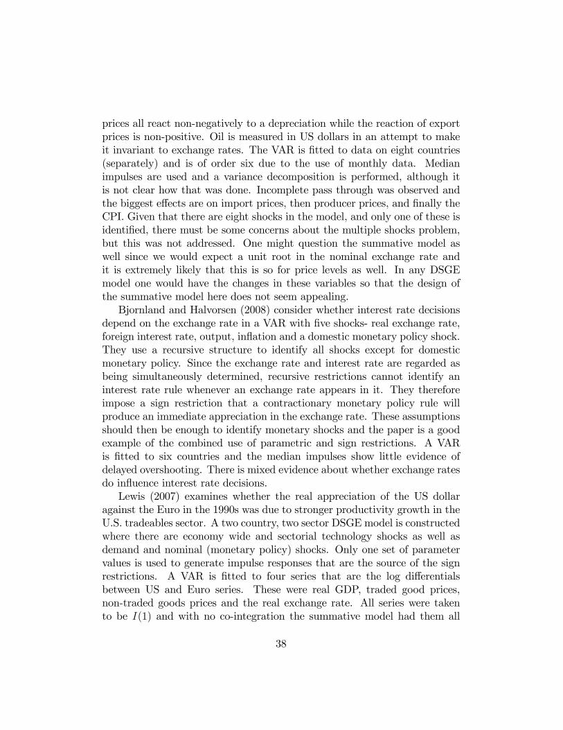
prices all react non-negatively to a depreciation while the reaction of exportprices is non-positive. Oil is measured in US dollars in an attempt to makeit invariant to exchange rates. The VAR is �tted to data on eight countries(separately) and is of order six due to the use of monthly data. Medianimpulses are used and a variance decomposition is performed, although itis not clear how that was done. Incomplete pass through was observed andthe biggest e¤ects are on import prices, then producer prices, and �nally theCPI. Given that there are eight shocks in the model, and only one of these isidenti�ed, there must be some concerns about the multiple shocks problem,but this was not addressed. One might question the summative model aswell since we would expect a unit root in the nominal exchange rate andit is extremely likely that this is so for price levels as well. In any DSGEmodel one would have the changes in these variables so that the design ofthe summative model here does not seem appealing.Bjornland and Halvorsen (2008) consider whether interest rate decisions

depend on the exchange rate in a VAR with �ve shocks- real exchange rate,foreign interest rate, output, in�ation and a domestic monetary policy shock.They use a recursive structure to identify all shocks except for domesticmonetary policy. Since the exchange rate and interest rate are regarded asbeing simultaneously determined, recursive restrictions cannot identify aninterest rate rule whenever an exchange rate appears in it. They thereforeimpose a sign restriction that a contractionary monetary policy rule willproduce an immediate appreciation in the exchange rate. These assumptionsshould then be enough to identify monetary shocks and the paper is a goodexample of the combined use of parametric and sign restrictions. A VARis �tted to six countries and the median impulses show little evidence ofdelayed overshooting. There is mixed evidence about whether exchange ratesdo in�uence interest rate decisions.Lewis (2007) examines whether the real appreciation of the US dollar

against the Euro in the 1990s was due to stronger productivity growth in theU.S. tradeables sector. A two country, two sector DSGE model is constructedwhere there are economy wide and sectorial technology shocks as well asdemand and nominal (monetary policy) shocks. Only one set of parametervalues is used to generate impulse responses that are the source of the signrestrictions. A VAR is �tted to four series that are the log di¤erentialsbetween US and Euro series. These were real GDP, traded good prices,non-traded goods prices and the real exchange rate. All series were takento be I(1) and with no co-integration the summative model had them all

38

appearing in di¤erenced form. Here there is an inconsistency with the DSGEmodel. All shocks in the VAR have been permanent e¤ects but the signrestrictions found from the DSGE model are for transitory shocks. Lewis,Table 3, gives enough sign restrictions to identify the shocks (these holdfor four quarters except for the e¤ects on the real exchange rate). Medianimpulses and variance decompositions are used and it is found that sectorialtechnology shocks explain about one �fth of the variation in the real exchangerate.13 What is striking however is that around one half of the variation isdue to nominal shocks, something out of line with the rest of the literature.Since there is no risk premium shock in the model, variation in the nominalexchange rate ( and hence the real rate) is probably being ascribed to nominalshocks by default.

4.5 Miscellaneous

Hau and Rey (2004) are interested in whether the portfolio re-balancing as-sociated with unhedged foreign equity leads to changes in equity returns,equity �ows and the exchange rate. They have a three variable VAR involv-ing those three variables for the US relative to �ve other countries. Dataare at a monthly frequency. Three shocks are to be identi�ed�equity price,exchange rate and equity �ow. Portfolio re-balancing after equity and ex-change rate shocks implies sign restrictions on the correlations between thevariables while an equity �ow shock also has predictions for the correlationsas well. Six sign restrictions are imposed. The problem then is what onecan learn from the study. Their conclusion is that the data "..are consis-tent with a dynamic rebalancing.." but this seems to re�ect a mis-conceptionabout the operation of sign restrictions, as seen in the following quotation""The decomposition of the variance-covariance matrix uses only three freeparameters ( three rotation angles) to �t a total of six theoretical moments,Rejection of one or more of the six conditional correlation implications by thedata is therefore possible" (p 130). This is incorrect. The six sign restrictionsare needed to identify the six unknown coe¢ cients in the SVAR. The three"rotation angles" ( �1; �2; �3) are not estimated from the data at all. Now it iscertainly possible that one could �nd that there are many models which areinconsistent with the sign restrictions, and that would indicate that there is

13Lewis notes in Table 4 that the contribution of the shocks to the variance of the realexchange rate sum to more than unity, a feature we noted earlier was likely to occur whenthese come from disparate models.

39

a con�ict of the data with portfolio re-balancing. But the impulse responsespresented are those from a unique model chosen from the set of models thatsatisfy the sign restrictions by using Uhlig�s penalty function. Consequently,portfolio balancing is imposed and one cannot learn anything about its exis-tence from the quantitative work they perform. One might learn somethingabout the strength of the e¤ect by considering the magnitudes of the impulseresponses selected, but these are biassed towards being strong by the use ofUhlig�s criterion.Fujita (2009) estimates a trivariate VAR consisting of quarterly US labour

market data on the job separation rate, the job �nding rate and vacancies.One shock is to be identi�ed - a negative "aggregate" shock. Given thatthere are identities linking the three basic variables to gross job separations,gross hires and the level of unemployment, it is possible to trace out impulseresponses to those variables after the VAR has been estimated. The neg-ative aggregate shock implies that unemployment changes are non-negativefor K periods and vacancies are not raised initially. These constitute thesign restrictions to identify the shock. As in other studies there is a poten-tial multiple shock problem and Fujita (2009) responds to this by retainingall of them, arguing that one is thereby getting the "average e¤ect" of theshock. This does not seem entirely satisfactory if there are many instancesof this occurring. Percentiles are presented in response to the multiple mod-els problem. A key element in the study is that the job separation rate isbeing treated as endogenously determined rather than made exogenous asin most models analyzing labour market dynamics, so that the SVAR beingestimated is novel. If one made the separation rate exogenous then unem-ployment dynamics would be quite di¤erent.Eickmeier et al. (2000) consider how bank loans respond to supply, de-

mand and monetary shocks in Germany and the Euro area. Four variablesappear in the VAR- real gdp, an interest rate, the price level and the stockof outstanding bank loans. Sign restrictions are like those on Tables 1 and 2( initially and for one period ahead) and no prediction is made about theirimpact on loans. Since only three shocks re identi�ed there is clearly a pos-sibility of a multiple shock problem and they allude to this in the paper, butseem to just retain all the shocks. They work with 500 models that satisfythe sign restrictions. To get these required 11515 draws for Germany and2616 for Europe which might suggest that the model is not that compatiblewith German data. They present variance decompositions which point tofairly equal contribution of shocks to loans. It is unclear how these decom-

40

positions were done given that there is a fourth unidenti�ed shock so thereis no reason to think it is uncorrelated with the three identi�ed shocks.Jarocinski and Smets are interested in the determinants of US house

prices. They have nine variables in a VAR- level of interest rate, interestrate spread, house investment to gdp, real consumption, real GDP, the gdpde�ator, real house prices, commodity prices and the money supply. Theseare all in logs except for the interest rates. There is also a version that usesdi¤erences of (the logs of) GDP, consumption, the GDP de�ator, commod-ity prices and money, and in which all di¤erenced variables are measuredrelative to their steady state values. The latter summative model is thenestimated using Bayesian methods with a prior on the steady state valuesand a Minnesota prior for the dynamics. The latter seems odd as it impliesa unit root in the series but, as these are growth rates, that does not seemappropriate. In any case this summative model is introduced but not usedmuch in the paper. Three shocks are identi�ed - housing demand, monetarypolicy and a "spread" shock. Restrictions are a combination of parametricand sign. There is not much discussion of the other six shocks and how theseare handled. This seems important since it was found that the three identi-�ed shocks had no in�uence on output, and that the housing demand shockwas the dominant contributor to housing investment and house prices.

5 Conclusion

When sign restriction work �rst began it was mainly about the identi�ca-tion of a single shock. Since then it has become popular to identify multipleshocks. Moreover the range of applications has grown from the initial focuson monetary policy. Given that sign information is rather weak we suspectthat it is best to utilize the restrictions in conjunction with parametric restric-tions and that seems to be an emerging tendency as well. A number of otherthemes also seem to be developing. One is that contemporaneous restric-tions might be preferable to imposing restrictions on longer lags. Anotheris that DSGE models are a useful way of �nding out likely sign restrictions,particularly as the number of variables in the VAR grows. We have tried toshow these tendencies in the review, and have also argued that more careoften needs to be taken in devising the model that is to summarize the data,a clear statement about whether shocks are permanent or transitory shouldbe provided, and an account of how the multiple models and multiple shocks

41

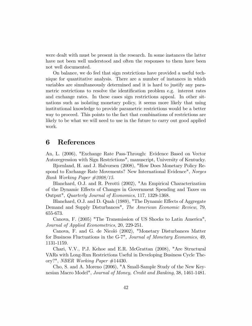
were dealt with must be present in the research. In some instances the latterhave not been well understood and often the responses to them have beennot well documented.On balance, we do feel that sign restrictions have provided a useful tech-

nique for quantitative analysis. There are a number of instances in whichvariables are simultaneously determined and it is hard to justify any para-metric restrictions to resolve the identi�cation problem e.g. interest ratesand exchange rates. In these cases sign restrictions appeal. In other sit-uations such as isolating monetary policy, it seems more likely that usinginstitutional knowledge to provide parametric restrictions would be a betterway to proceed. This points to the fact that combinations of restrictions arelikely to be what we will need to use in the future to carry out good appliedwork.

6 References

An, L. (2006), "Exchange Rate Pass-Through: Evidence Based on VectorAutoregression with Sign Restrictions", manuscript, University of Kentucky.Bjornland, H. and J. Halvorsen (2008), "How Does Monetary Policy Re-

spond to Exchange Rate Movements? New International Evidence", NorgesBank Working Paper #2008/15.Blanchard, O.J. and R. Perotti (2002), "An Empirical Characterization

of the Dynamic E¤ects of Changes in Government Spending and Taxes onOutput", Quarterly Journal of Economics, 117, 1329-1368.Blanchard, O.J. and D. Quah (1989), "The Dynamic E¤ects of Aggregate

Demand and Supply Disturbances", The American Economic Review, 79,655-673.Canova, F. (2005) "The Transmission of US Shocks to Latin America",

Journal of Applied Econometrics, 20, 229-251.Canova, F. and G. de Nicoló (2002), "Monetary Disturbances Matter

for Business Fluctuations in the G-7", Journal of Monetary Economics, 49,1131-1159.Chari, V.V., P.J. Kehoe and E.R. McGrattan (2008), "Are Structural

VARs with Long-Run Restrictions Useful in Developing Business Cycle The-ory?", NBER Working Paper #14430.Cho, S. and A. Moreno (2006), "A Small-Sample Study of the New Key-

nesian Macro Model", Journal of Money, Credit and Banking, 38, 1461-1481.

42

Canova, F. and E. Pappa (2007), "Price Di¤erentials in Monetary Unions:The Role of Fiscal Shocks", Economic Journal, 117, 713-737.Canova, F. and M. Paustian (2007), "Measurement with Some Theory:

Using Sign Restrictions to Evaluate Business Cycle Models", manuscript,ICREA_UPF.Christiano, L.J., M. Eichenbaum, and C. Evans (1997), "Monetary Policy

Shocks: What Have We Learned and to What End?", Manuscript, FederalReserve Bank of Chicago.Clarida, R. and J. Gali (1994), "Sources of Exchange Rate Fluctuations:

How Important are Nominal Shocks?", Carnegie-Rochester Conference onPublic Policy, 41, 1-56.Dedola, L. and S. Neri (2006), "What Does a Technology Shock Do? A

VAR Analysis with Model Based Sign Restrictions", ECB Working Paper#705.Dungey, M. and R.A. Fry, (2009), "Identifying Fiscal andMonetary Policy

in a Structural VAR", Economic Modelling, 26, 1147-1160.Eichenbaum, M. and C.L. Evans, (1995), "Some Empirical Evidence on

the E¤ects of Shocks to Monetary Policy on Exchange Rates", The QuarterlyJournal of Economics, 110, 975-1009,Eickmeier, S., B. Hofmann and A. Worms (2009), "Macroeconomic Fluc-

tuations and Bank Lending: Evidence for Germany and the Euro Area",German Economic Review, 10, 193-223.Farrant, K. and G. Peersman (2006), "Is the Exchange Rate a Shock Ab-

sorber or a Source of Shocks? New Empirical Evidence", Journal of Money,Credit and Banking, 38, 939-961Faust, J. (1998), "The Robustness of Identi�ed VAR Conclusions about

Money", Carnegie-Rochester Series on Public Policy, 49, 207-244.Faust, J. and E.M. Leeper (1997), "When Do Long-Run Identifying Re-

strictions Give Reliable Results?", Journal of Business and Economic Sta-tistics, 15, 345-353.Faust, J. and J.H. Rogers (2003), "Monetary Policy�s Role in Exchange

Rate Behavior", Journal of Monetary Economics, 50, 1403-1424.Fisher, J.D.M. (2006), "The Dynamic E¤ects of Neutral and Investment-

Speci�c Technology Shocks", Journal of Political Economy, 114, 413-451.Fry,R. and A. R. Pagan (2005), "Some Issues in Using VARs for Macro-

econometric Research", CAMA Working Paper #19.Francis, N., M.T. Owyang and J.E. Roush (2005), "A Flexible Finite-

Horizon Identi�cation of Technology Shocks", Board of the Governors of the

43

Federal Reserve System, International Finance Discussion Papers #832.Fry, R.A. and A.R. Pagan (2005), "Some Issues in Using VARs for Macro-

econometric Research", CAMA Working Paper #19.Fry, R.A. and A.R. Pagan (2007), "Some Issues in Using Sign Restrictions

for Identifying Structural VARs", NCER Working Paper #14.Fujita, S. (2009), "Dynamics of Worker Flows and Vacancies: Evidence

from the Sign Restriction Approach", Journal of Applied Econometrics, forth-coming.Gali, J. (1999), "Technology, Employment, and the Business Cycle: Do

Technology Shocks Explain Aggregate Fluctuations?", The American Eco-nomic Review, 89, 249�271.Grilli, V. and N. Roubini (1995), "Liquidity and Exchange-Rates: Puz-

zling Evidence from the G-7 Countries", manuscript, Yale University.Grilli, V. and N. Roubini (1996), "Liquidity Models in Open Economies:

Theory and Empirical Evidence", European Economic Review, 40, 847-859.Hau, H. and H. Rey (2004), "Can Portfolio Rebalancing Explain the

Dynamics of Equity Returns, Equity Flows and Exchange Rates", AmericanEconomic Review, 94, 126-133.Jarocinski, M. and F.R. Smets (2008), "House Prices and the Stance of

Monetary Policy", Federal Reserve Bank of St Louis Review, July/August2008, 339-365.Justiniano, A. and B. Preston (2008), "Can Structural Small Open Econ-

omy Models Account for the In�uence of Foreign Disturbances?", NBERWorking Paper #14547.Kapetanios, G., A.R. Pagan and A. Scott (2007), "Making a Match: Com-

bining Theory and Evidence in Policy-Oriented Macroeconomic Modelling",Journal of Econometrics, 136, 565-594.Kilian, L. and D. Murphy (2009), "Why Agnostic Sign Restrictions are

Not Enough: Understanding the Dynamics of Oil Market VAR Models",manuscript, University of Michigan.Leamer (1978), Speci�cation Searches and Ad-Hoc Inference for Nonex-

perimental Data, John Wiley, New YorkLevtchenkova, S. and A.R. Pagan and J.C. Robertson (1998), �Shocking

Stories�, Journal of Economic Surveys, 12, 507-532.Mountford, A. (2005), "Leaning into the Wind: A Structural VAR Inves-

tigation of UK Monetary Policy", Oxford Bulletin of Economics and Statis-tics, 67, 597-621.

44

Mountford, A. and H. Uhlig (2005), "What are the E¤ects of Fiscal Pol-icy Shocks", Discussion Paper 2005-039, SFB 649, Humboldt-Universitat,Berlin.Mountford, A. and H. Uhlig (2008), "What are the E¤ects of Fiscal Policy

Shocks?", NBER Working Paper #14551.Pagan, A.R. and M.H. Pesaran (2008), �Econometric Analysis of Struc-

tural Systems with Permanent and Transitory Shocks�, Journal of EconomicDynamics and Control, 32, 3376-3395.Pagan, A.R. and J. Robertson, (1998), �Structural Models of the Liquid-

ity E¤ect�, Review of Economics and Statistics, 80, 202-217.Paustian, M. (2007), "Assessing Sign Restrictions" The B.E. Journal of

Macroeconomics, 7, 1-37.Peersman, G. (2005), "What Caused the Early Millenium Slowdown?

Evidence Based on Autoregressions", Journal of Applied Econometrics, 20,185-207.Peersman, G. and R. Straub (2004), "Technology Shocks and Robust Sign

Restrictions in a Euro Area SVAR", ECB Working Paper #373.14

Peersman, G. and R. Straub (2009), "Technology Shocks and RobustSign Restrictions in a Euro Area SVAR", International Economic Review,50, 727-750.15

Peersman, G. and R. Straub (2006), "Putting the New Keynesian Modelto a Test", IMF Working Paper, 06/135.Preston, A.J. (1978), "Concepts of Structure and Model Identi�ability

for Econometric Systems" in A.R. Bergstrom et al., Stability and In�ation(Wiley, 1978), 275�297.Quenouille, M.H. (1957), The Analysis of Multiple Time Series, Gri¢ n�s

Statistical Monograohs and Course No 1 (Gri¢ n, London).Ra�q, M.S. and S.K. Mallick (2008), "The E¤ects of Monetary Policy on

Output in EMU3 A Sign Restriction Approach", Journal of Macroeconomics,30, 1756-1791.Rubio-Ramirez, J.F., D.F.Waggoner and T. Zha (2005), "Markov-Switching

Structural Vector Autoregressions: Theory and Application",Working Paper#2005-27, Federal Reserve Bank of Atlanta.Ru¤er, R., M. Sanchez and J-G Shen (2007), "Emerging Asia�s Growth

and Integration: How Autonomous are Business Cycles", ECB Working Pa-

14delete this when changed to 200915Change peersman and staub 2004 to 2009

45

per #715.Sanchez, M. (2007), "What Drives Business Cycles and International

Trade in Emerging Market Economies?", ECB Working Paper #730.Scholl, A. and H. Uhlig (2005), "New Evidence on the Puzzles: Results

from Agnostic Identi�cation of Monetary Policy and Exchange Rates", Dis-cussion Paper 2005-037, SFB 649, Humboldt-Universitat, Berlin.Scholl, A. and H. Uhlig, (2008), "New Evidence on the Puzzles: Re-

sults from Agnostic Identi�cation on Monetary Policy and Exchange Rates",Journal of International Economics, 76, 1-13.16

Shapiro, M.D. and M.W.Watson (1988), "Sources of Business Cycle Fluc-tuations", in S. Fischer (ed) NBER Macroeconomics Annual 1988, 111-148.Sims, C.A. (1980), �Macroeconomics and Reality", Econometrica, 48, 1-

48.Uhlig, H. (2005), "What are the E¤ects of Monetary Policy on Output?

Results from an Agnostic Identi�cation Procedure", Journal of MonetaryEconomics, 52, 381-419.Vargas-Silva, C. (2008), "Monetary Policy and US Housing: A VAR Im-

posing Sign Restrictions", Journal of Macroeconomics, 30, 977-990.Wallis, K.F. (1977), "Multiple Time Series and the Final Form of Econo-

metric Models", Econometrica, 45, 1481-1497.Wold, H.O. (1951), "Dynamic Systems of the Recursive Type- Economic

and Statistical Aspects", Sankhya, 11 (1951), 205-216.Zellner, A. and F. Palm (1974), "Time Series Analysis and Simultaneous

Equation Econometric Models", Journal of Econometrics, 2, 17-54.

16this has changed from 2005 to 2009

46

7 Appendix

The table is a sub-set of published studies and adopts a taxonomy whichdistinguishes between cases where only sign restrictions are used (often thereare mixtures of sign and parametric restrictions), the type of shock (perma-nent or transitory), the number of shocks identi�ed, and whether the signrestrictions come from a formal model or not.

47

Table 1:

Table 3 Summary of Empirical VAR Studies Employing Sign Restrictions

Fluctuations Ru¤er et al (2007) STNIPeersman (2005) STNISanchez (2007) STNF

Ex Rate Scholl/Uhlig (2005) STNIFarrant/Peersman (2006) STNFBjornland/Halvorsen (2008) MTNILewis (2007) STNFAn(2006) STOI

Fiscal Policy Mountford/Uhlig (2005) STNIDungey/Fry(2008) MPTNI

Housing Jarocinski/Smets (2008) MTNIVargas-Silva (2008) STOI

Monetary Policy Faust (1998) STOICanova/De Nicoló (2002) STOFMountford (2005) STNIScholl/Uhlig (2005) STNIUhlig (2005) STOIRa�q/Mallick (2008) STOI

Technology Francis/Owyang/Theodorou (2003) MPTOIPeersman/Straub (2004) STNFFrancis/Owyang/Roush (2005) MPTOFDedola/Neri (2007) SPTOFChari/Kehoe/McGrattan (2008) MPTNF

Various Hau and Rey (2004) STNFEickmeier/Ho¤mann/Worms (2006) STNIFujita(2009) STOI

Restriction Type: S= Sign only, M = Mixed

Shock Types: P=Permanent, T= Transitory

Number of Shocks: O=One only, N=Numerous

Restriction Source: F=Formal, I= Informal

48