Signal Processing Tools for Radio

Astronomy

Alle-Jan van der Veen and Stefan J. Wijnholds

Abstract Radio astronomy is known for its very large telescope dishes, butis currently making a transition towards the use of large numbers of smallelements. For example, the Low Frequency Array, commissioned in 2010, usesabout 50 stations, each consisting of at least 96 low band antennas and 768high band antennas. For the Square Kilometre Array, planned for 2024, thenumbers will be even larger. These instruments pose interesting array sig-nal processing challenges. To present some aspects, we start by describinghow the measured correlation data is traditionally converted into an image,and translate this into an array signal processing framework. This paves theway for a number of alternative image reconstruction techniques, such asa Weighted Least Squares approach. Self-calibration of the instrument is re-quired to handle instrumental effects such as the unknown, possibly directiondependent, response of the receiving elements, as well a unknown propaga-tion conditions through the Earth’s troposphere and ionosphere. Array signalprocessing techniques seem well suited to handle these challenges. The factthat the noise power at each antenna element may be different motivates theuse of Factor Analysis, as a more appropriate alternative to the eigenvaluedecomposition that is commonly used in array processing. Factor Analysisalso proves to be very useful for interference mitigation. Interestingly, imagereconstruction, calibration and interference mitigation are often intertwinedin radio astronomy, turning this into an area with very challenging signalprocessing problems.

A.J. van der VeenTU Delft, Fac. EEMCS, Mekelweg 4, 2628 CD Delft, The Netherlandse-mail: a.j.vanderveen@tudelft.nl

S.J. WijnholdsNetherlands Institute for Radio Astronomy (ASTRON), Oude Hoogeveensedijk 4,7991 PD Dwingeloo, The Netherlandse-mail: wijnholds@astron.nl

1

1 Introduction

Astronomical instruments measure cosmic particles or electromagnetic wavesimpinging on the Earth. Astronomers use the data generated by these in-struments to study physical phenomena outside the Earth’s atmosphere. Inrecent years, astronomy has transformed into a multi-modal science in whichobservations at multiple wavelengths are combined. Figure 1 provides a niceexample showing the lobed structure of the famous radio source Cygnus Aas observed at 240 MHz with the Low Frequency Array (LOFAR) overlaidby an X-Ray image observed by the Chandra satellite, which shows a muchmore compact source.

Such images are only possible if the instruments used to observe differentparts of the electromagnetic spectrum provide similar resolution. Since theresolution is determined by the ratio of observed wavelength and aperturediameter, the aperture of a radio telescope has to be 5 to 6 orders of magni-tude larger than that of an optical telescope to provide the same resolution.This implies that the aperture of a radio telescope should have a diameterof several hundreds of kilometers. Most current and future radio telescopes

Fig. 1 Radio image of Cygnus A observed at 240 MHz with the Low FrequencyArray (showing mostly the lobes left and right), overlaid over an X-Ray image of thesame source observed by the Chandra satellite (the fainter central cloud). (Courtesyof Michael Wise and John McKean.)

therefore exploit interferometry to synthesize a large aperture from a numberof relatively small receiving elements.

An interferometer measures the correlation of the signals received by twoantennas spaced at a certain distance. After a number of successful experi-ments in the 1950s and 1960s, two arrays of 25-m dishes were built in the1970s: the 3 km Westerbork Synthesis Radio Telescope (WSRT, 14 dishes)in Westerbork, The Netherlands and the 36 km Very Large Array (VLA, 27movable dishes) in Socorro, New Mexico, USA. These telescopes use Earthrotation to obtain a sequence of correlations for varying antenna baselines,resulting in high-resolution images via synthesis mapping. A more extensivehistorical overview is presented in [37].

The radio astronomy community is currently commissioning a new genera-tion of radio telescopes for low frequency observations, including the Murchi-son Widefield Array (MWA) [24] in Western Australia and the Low FrequencyArray (LOFAR) [42] in Europe. These telescopes exploit phased array tech-nology to form a large collecting area with ∼1000 to ∼50,000 receiving ele-ments. The community is also making detailed plans for the Square KilometreArray (SKA), a future radio telescope that should be one to two orders ofmagnitude more sensitive than any radio telescope built to date [12]. Thiswill require millions of elements to provide the desired collecting area of orderone square kilometer.

The individual antennas in a phased array telescope have an extremelywide field-of-view, often the entire visible sky. This poses a number of signalprocessing challenges, because certain assumptions that work well for smallfields-of-view (celestial sphere approximated by a plane, homogenous prop-agation conditions over the field-of-view), are no longer valid. Furthermore,the data volumes generated by these new instruments will be huge and willhave to be reduced to manageable proportions by a real-time automated dataprocessing pipeline. This combination of challenges led to a flurry of researchactivity in the area of array calibration, imaging and RFI mitigation, whichare often intertwined in the astronomical data reduction.

The goal of calibration is to find the unknown instrumental, atmosphericand ionospheric disturbances. The imaging procedure should be able to applyappropriate corrections based on the outcome of the calibration process toproduce a proper image of the sky. In this chapter, we review some of the arrayprocessing techniques that have been proposed for use in the data reductionpipelines, some of which are now being used in the LOFAR data reductionpipelines.

2 Notation

Matrices and vectors will be denoted by boldface upper-case and lower-casesymbols, respectively. Entries of a matrix A are denoted by aij , and its

columns by ai. Overbar (·) denotes complex conjugation. The transpose op-erator is denoted by T , the complex conjugate (Hermitian) transpose by H

and the Moore-Penrose pseudo-inverse by †. For matrices A of full columnrank, i.e., AHA invertible, this is equal to the left inverse:

A† = (AHA)−1AH . (1)

The expectation operator is denoted by E{·}.We will multiply matrices in many different ways. Apart from the usual

multiplication AB, we will use A � B to denote the element-wise matrixmultiplication (Hadamard product), and A ⊗ B to denote the Kroneckerproduct,

A ⊗B =

a11B a12B · · ·a21B a22B · · ·

......

. . .

.

We will also use the Khatri-Rao or column-wise Kronecker product of twomatrices: let A = [a1, a2, · · · ] and B = [b1,b2, · · · ], then

A ◦B = [a1 ⊗ b1, a2 ⊗ b2, · · · ] .

Depending on the context, diag(·) converts a vector to a diagonal matrix withthe elements of the vector placed on the main diagonal, or converts a generalmatrix to a diagonal matrix by selecting its main diagonal. Further, vec(·)converts a matrix to a vector by stacking the columns of the matrix.

Properties of Kronecker products are listed in, e.g., [29]. We will frequentlyuse the following properties:

(A⊗ B)(C⊗D) = AC ⊗BD (2)

vec(ABC) = (CT ⊗A)vec(B) (3)

vec(A diag(b)C) = (CT ◦A)b (4)

Property (3) is used to move a matrix B from the middle of an equation tothe right of it, exploiting the linearity of the product. Property (4) is a specialcase of it, to be used if B is a diagonal matrix: in that case vec(B) has manyzero entries, and we can omit the corresponding columns of CT ⊗A, leavingonly the columns of the Khatri-Rao product CT ◦A.

A special case of (3) is

vec(aaH ) = a ⊗ a (5)

which shows how a rank-1 matrix aaH is related to a vector with a specific“Kronecker structure”.

3 Basic concepts of interferometry and image formation

The concept of interferometry is illustrated in figure 2. An interferometermeasures the spatial coherency of the incoming electromagnetic field. This isdone by correlating the signals from the individual receivers with each other.The correlation of each pair of receiver outputs provides the amplitude andphase of the spatial coherence function for the baseline defined by the vectorpointing from the first to the second receiver in a pair. In radio astronomy,these correlations are called the visibilities.

3.1 Data acquisition

Mathematically, the correlation process is described as follows. Assume thatthere are J array elements (telescopes). The RF signal xj(t) from the jthtelescope is first moved to baseband where it is denoted by xj(t), then sam-pled and split into narrow subbands, e.g., of 100 kHz each, such that the“narrowband condition” holds. This condition states that the maximal geo-metrical delay across the array should be fairly representable by a phase shiftof the complex baseband signal, and this property is discussed in more detailin the next subsection.

The resulting signal is called xj(n, k), for the jth telescope, nth time bin,and for the subband frequency centered at RF frequency fk. The J signalsare stacked into a J × 1 vector x(n, k).

A single correlation matrix is formed by “integrating” (summing) thecrosscorrelation products x(n, k)xH (n, k) over N subsequent samples,

x2(t)g2g1

geometricdelay

xJ (t)gJbaseline

FOV

x1(t)

Fig. 2 Schematic overview of a radio interferometer.

Rm,k =1

N

mN−1∑

n=(m−1)N

x(n, k)xH (n, k) , (6)

where m is the index of the corresponding “short-term interval” (STI) overwhich is correlated. The processing chain is summarized in figure 3.

The duration of a STI depends on the stationarity of the data, whichis limited by factors like Earth rotation and the diameter of the array. Forthe Westerbork array, a typical value for the STI is 10 to 30 s; the totalobservation can last for up to 12 hours. The resulting number of samples N ina snapshot observation is equal to the product of bandwidth and integrationtime and typically ranges from 103 (1 s, 1 kHz) to 106 (10 s, 100 kHz) inradio astronomical applications.

3.2 Complex baseband signal representation

Before we can derive a data model, we need to include some more detailson the RF to baseband conversion. In signal processing, signals are usuallyrepresented by their low pass equivalents, which is a suitable representationfor narrowband signals in a digital communication system, and also applicablein the radio astronomy context. A real valued bandpass signal with centerfrequency fc may be written as

s(t) = real{s(t)ej2πfct} = x(t) cos 2πfct − y(t) sin 2πfct (7)

where s(t) = x(t) + jy(t) is the complex envelope of the RF signal s(t), alsocalled the complex baseband signal. The real and imaginary parts, x(t) andy(t), are called the in-phase and quadrature components of the signal s(t). Inpractice, they are generated by multiplying the received signal with cos 2πfctand sin 2πfct followed by low-pass filtering.

BBfilter

bank

x(t) x(n, k)

100 kHz10 µs

x(n, k)x(n, k)H

10 MHz

P

10 s

10 s

Rm,k

x1(t)

xJ(t)

RFto

Fig. 3 The processing chain to obtain covariance data.

Suppose that the bandpass signal s(t) is delayed by a time τ . This can bewritten as

sτ (t) := s(t − τ) = real{s(t − τ)ej2πfc(t−τ)} = real{s(t − τ)e−j2πfcτej2πfct} .

The complex envelope of the delayed signal is thus sτ (t) = s(t − τ)e−j2πfcτ .Let W be the bandwidth of the complex envelope (the baseband signal) andlet S(f) be its Fourier transform. We then have

s(t − τ) =

∫ W/2

−W/2

S(f)e−j2πfτej2πftdf ≈∫ W/2

−W/2

S(f)ej2πftdf = s(t)

where the approximation e−j2πfτ ≈ 1 is valid if |2πfτ | � 1 for all frequencies|f | ≤ W

2 . Ignoring a factor π, the resulting condition Wτ � 1 is calledthe narrowband condition. Under this condition, we have for the complexenvelope sτ (t) of the delayed bandpass signal sτ (t) that

sτ (t) ≈ s(t)e−j2πfcτ for Wτ � 1 .

The conclusion is that, for narrowband signals, time delays smaller thanthe inverse bandwidth may be represented as phase shifts of the complexenvelope. Phased array processing heavily depends on this step. For radioastronomy, the maximal delay τ is equal to the maximal geometric delay,which can be related to the diameter of the array. The bandwidth W is thebandwidth of each subband fk in the RF processing chain that we discussedin the previous subsection.

3.3 Basic data model

We return to the radio astronomy context. For our purposes, it is convenientto model the sky as consisting of a collection of Q spatially discrete pointsources, with sq(n, k) the signal of the qth source at time sample n andfrequency fk.

In the simplest case, the signal received at the first antenna is a direct sumof these source signals, and the signal at the jth antenna is a sum of delayedsignals, where the delays are geometric delays that depend on the directionunder which each of the signals are observed. In the previous subsection, wesaw that under the narrowband condition a delay of a narrowband signals(t, k) by τ can be represented by a phase shift:

sτ (t, k) = e−j2πfkτs(t, k)

which takes the form of a multiplication of s(t, k) by a complex number.Let [xj , yj , zj ]

T be the location of the jth antenna, with respect to the first

antenna. Further, let pq be a unit-length direction vector pointing into thedirection of the qth source.

The geometrical delay τ at antenna j for a signal coming from direction pq

can be computed as follows. For a signal traveling directly from antenna 1 toantenna j, the delay is the distance between both antennas, divided by c, thespeed of light. For any other direction, the delay depends on the cosine of theangle of incidence (compared to the baseline vector), and is thus describedby the inner product of the location vector with the direction vector,

τ =[xj , yj , zj ]pq

c.

Overall, the phase factor representing the geometric delay is

e−j2πfkτ = e−jzTj pq , zj =

2πfk

c

xj

yj

zj

.

Here, we have introduced zj as a normalized location vector, assuming z1 = 0

is the location of the first antenna (i.e., the phase reference). As the Earthrotates, the relative locations of the telescopes are also moving, hence zj is afunction of sample time n (and of fk, due to the normalization), and we writeit as zj(n, k). The coordinates of source direction vectors pq are expressed as1

(`, m, n), where `, m are direction cosines, and n =√

1 − `2 − m2 due to thenormalization. There are several conventions and details regarding coordinatesystems [37], but they are not of concern for us here.

Taking the phase factors into account, we can model the received signalvector x(n, k) as

x(n, k) =

Q∑

q=1

aq(n, k)sq(n, k) + n(n, k) (8)

where aq(n, k) is called the “array response vector” for the qth source, consist-ing of the phase multiplication factors, and n(n, k) is an additive noise vector,due to thermal noise at the receiver. We will model sq(n, k) and n(n, k) asbaseband complex envelope representations of zero mean wide sense station-ary white Gaussian random processes sampled at the Nyquist rate.

With the above discussion, the array response vector is modeled (for anideal receiver) as

aq(n, k) = e−jZ(n,k)T pq , Z(n, k) = [z1(n, k), · · · , zJ(n, k)] . (9)

For convenience of notation, we will in future usually drop the dependenceon the frequency fk (index k) from the notation.

1 with abuse of notation, as m, n are not related to the time variables used earlier.

Previously, in (6), we defined correlation estimates Rm as the output ofthe data acquisition process, where the time index m corresponds to the mthshort term integration interval (STI), such that (m − 1)N ≤ n ≤ mN . Dueto Earth rotation, the vector aq(n) changes slowly with time, but we assumethat within an STI it can be considered constant and can be represented, withsome abuse of notation, by aq(m). In that case, x(n) is wide sense stationaryover the STI, and a single STI autocovariance is defined as

Rm = E{x(n)xH(n)} , m =⌈ n

N

⌉

(10)

where Rm has size J ×J . Each element of Rm represents the interferometriccorrelation along the baseline vector between the two corresponding receivingelements. It is estimated by STI sample covariance matrices Rm defined in(6), and our stationarity assumptions imply E{Rm} = Rm.

If we consider only a single signal from direction pq and look at entry (i, j)of Rm, then its value is

(Rm)i,j = E{xi(n)xj(n)} = σ2qe−j(zi(m)−zj (m))T pq . (11)

The vector zi(m) − zj(m) is the baseline: the (normalized) vector pointingfrom telescope i to telescope j. In radio astronomy, it is usually expressed incoordinates denoted by (u, v, w). The objective in telescope design is often tohave as many different baselines as possible. In that case the entries of Rm

are different and non-redundant. As the Earth turns, the baselines also turn,thus giving rise to new baseline directions. We will see later that the set ofbaselines during an observation determines the spatial sampling function bywhich the incoming wave field is sampled, with important implications onthe quality of the resulting image.

If we generalize now (11) to Q sources and add zero mean noise, uncorre-lated from antenna to antenna, as in the signal model (8), we obtain what isknown as the measurement equation, or covariance data model,

Rm = AmΣsAHm + Σn, (12)

where Am = [a1(m), · · · , aQ(m)]

Σs = diag{[σ21 , · · · , σ2

Q]}Σn = E{n(n)nH(n)} = diag{[σ2

n,1, · · · , σ2n,J ]} .

Here, σ2q = E{|sq(n, k)|2} is the variance of the qth source, Σs is the cor-

responding signal covariance matrix, and Σn is the noise covariance matrix.(With abuse of notation, subscript n is now used to signify “noise”.) Noise isassumed to be independent but not evenly distributed across the array. Thenoise variances σ2

n,j are considered unknown.

Under ideal circumstances, the array response matrix Am is just a phasematrix: its columns are given by the vectors aq(m) in (9), and its entriesexpress the phase shifts due to the geometrical delays associated with thearray and source geometry. We will later generalize this and introduce di-rectional disturbances due to non-isotropic antennas, unequal antenna gains,and disturbances due to atmospheric effects.

3.4 Image formation for the ideal data model

Ignoring the additive noise and using the ideal array response matrix Am,the measurement equation (12), in its simplest form, can be written as

(Rm)i,j =

Q∑

q=1

I(pq) e−j (zi(m)−zj(m))T pq (13)

where (Rm)i,j is the correlation between antennas i and j at STI interval m,I(pq) = σ2

q is the brightness (power) of the source in direction pq , zi(m) isthe normalized location vector of the ith antenna at STI m, and pq is theunit direction vector (position) of the qth source.

The function I(p) is the brightness image (or map) of interest: it is thisfunction that is shown when we refer to a radio-astronomical image like figure1. It is a function of the direction vector p: this is a 3D vector, but due to itsnormalization it depends on only two parameters. We could e.g., show I(·)as function of the direction cosines (`, m), or of the corresponding angles.

For our discrete point-source model, the brightness image is

I(p) =

Q∑

q=1

σ2q δ(p − pq) (14)

where δ(·) is a Kronecker delta, and the direction vector p is mapped to thelocation of “pixels” in the image (various transformations are possible). Onlythe pixels pq are nonzero, and have value equal to the source variance σ2

q .Equation (13) describes the relation between the visibility model and the

desired image, and it has the form of a Fourier transform; it is known in radioastronomy as the Van Cittert-Zernike theorem [33, 37]. Image formation (map

making) is essentially the inversion of this relation. Unfortunately, we haveonly a finite set of observations, therefore we can only obtain a dirty image:if we apply the inverse Fourier transformation to the measured correlationdata, we obtain

ID(p) :=∑

i,j,m

(Rm)ij ej (zi(m)−zj (m))T p . (15)

−40 −30 −20 −10 0 10 20 30−30

−20

−10

0

10

20

30

40

East ← x → West

Sou

th ←

y →

Nor

th

East ← l → West

Sou

th ←

m →

Nor

th

−1−0.500.51−1

−0.5

0

0.5

1

−40

−35

−30

−25

−20

−15

−10

−5

0

Fig. 4 (a) Coordinates of the antennas in a LOFAR station, which defines the spatialsampling function, and (b) the resulting dirty beam.

In terms of the measurement data model (13), the “expected value” of theimage is obtained by replacing Rm by Rm, or

ID(p) :=∑

i,j,m

(Rm)i,j ej (zi(m)−zj(m))T p

=∑

i,j,m

∑

q

σ2q ej (zi(m)−zj(m))T (p−pq)

=∑

q

I(pq) B(p − pq)

= I(p) ∗ B(p) (16)

where the dirty beam is given by

B(p) :=∑

i,j,m

ej (zi(m)−zj(m))T p . (17)

The dirty image ID(p) is the desired image I(p) convolved with the dirtybeam B(p): every point source excites a beam B(p − pq) centered at itslocation pq . Note that B(p) is a known function: it only depends on thelocations of the telescopes, or rather the set of telescope baselines zi(m) −zj(m).

An example of a set of antenna coordinates and the corresponding dirtybeam is shown in figure 4. This is for a single low-band LOFAR station anda single STI and frequency bin. The dirty beam has heavy sidelobes as highas −10 dB. A resulting dirty image is shown in figure 5. In this image, wesee the complete sky, in (`, m) coordinates, where the reference directionis pointing towards zenith. The strong visible sources are Cassiopeia A andCygnus A, also visible is the milky way, ending in the north polar spur (NPS)and, weaker, Virgo A. In the South, the Sun is visible as well. The image was

East ← l → West

Sou

th ←

m →

Nor

th

DFT image

−1−0.500.51−1

−0.8

−0.6

−0.4

−0.2

0

0.2

0.4

0.6

0.8

1

0

0.2

0.4

0.6

0.8

1

1.2

1.4

1.6

Fig. 5 Dirty image following (16), using LOFAR station data.

obtained by averaging 25 STIs, each consisting of 10 s data in 25 frequencychannels of 156 kHz wide taken from the band 45–67 MHz, avoiding thelocally present radio interference. As this shows data from a single LOFARstation, with a relatively small maximal baseline (65 m), the resolution islimited and certainly not representative of the capabilities of the full LOFARarray.

The dirty beam is essentially a non-ideal point spread function due to finiteand non-uniform spatial sampling: we only have a limited set of baselines.The dirty beam usually has a main lobe centered at p = 0, and many sidelobes. If we would have a large number of telescopes positioned in a uniformrectangular grid, the dirty beam would be a 2-D sinc-function (similar to aboxcar taper in time-domain sampling theory). The resulting beam size is in-versely proportional to the aperture (diameter) of the array. This determinesthe resolution in the dirty image. The sidelobes of the beam give rise to con-fusion between sources: it is unclear whether a small peak in the image iscaused by the main lobe of a weak source, or the sidelobe of a strong source.Therefore, attempts are made to design the array such that the sidelobes arelow. It is also possible to introduce weighting coefficients (“tapers”) in (16)to obtain an acceptable beamshape.

Another aspect is the summation over m (STI intervals) in (17), wherethe rotation of the Earth is used to obtain essentially many more antennabaselines. The effect of this is that the sidelobes tend to get averaged out, tosome extent. Many images are also formed by averaging over a small numberof frequency bins (assuming the σ2

q are constant over these frequency bins),

which enters into the equations in exactly the same way: Replace zi(m) byzi(m, k) and also sum over the frequency index k.

4 Deconvolution algorithms for image formation

Deconvolution is the process of recovering I(·) from ID(·) using knowledgeof the dirty beam, and thus to obtain the original high-resolution, “clean”image. A standard algorithm for doing this is CLEAN [15] and variants; how-ever, many other algorithms are possible, depending on the underlying modelassumptions and in a trade-off between accuracy and numerical complexity.

After a telescope has been designed and built, deconvolution is the mostimportant step in image formation. It can increase the dynamic range (ra-tio between powers of the strongest and the weakest features in the image)by several orders of magnitude. However, the numerical complexity is oftenlarge, and high-resolution images require dedicated hardware solutions andsometimes even supercomputers. This section will describe some of the algo-rithms for deconvolution. Additional overviews are available in [8, 9, 19, 22],as well as in the books [37, 2].

4.1 The CLEAN algorithm

A popular method for deconvolution is the CLEAN algorithm [15]. From thedirty image ID(p) and the known dirty beam B(p), the desired image I(p)is obtained via a sequential Least Squares fitting method. The algorithm isbased on the assumption that the sky is mostly empty, and consists of a setof discrete point sources. The brightest source is estimated first, its contri-bution is subtracted from the dirty image, then the next brightest source issubtracted, etc.

The algorithm further assumes that B(p) has its peak at the origin. Insidethe loop, a candidate location pq is selected as the location of the largestpeak in ID(p), the corresponding power σ2

q is estimated, and subsequently asmall multiple of σ2

qB(p − pq) is subtracted from ID(p). The objective is tominimize the residual, until it converges to the noise level:

q = 0while ID(p) is not noise-like:

q = q + 1pq = arg maxp ID(p)σ2

q = ID(pq)/B(0)ID(p) := ID(p) − γσ2

qB(p − pq) , ∀pIclean(p) = ID(p) +

∑

q γσ2qBsynth(p − pq), ∀p .

The scaling parameter γ ≤ 1 is called the loop gain; for accurate convergenceit should be small because the estimated location of the peak is at a gridpoint, whereas the true location of the peak may be in between grid points.Bsynth(p) is a “synthetic beam”, usually a Gaussian bell-shape with aboutthe same beam width as the main lobe of the dirty beam; it is introduced tomask the otherwise high artificial resolution of the image.

In current imaging systems, instead of the subtractions on the dirty image,it is considered more accurate to do the subtractions on the covariance dataRm instead,

Rm := Rm − γσ2qaq(m)aq(m)H

and then to recompute the dirty image. For efficiency, usually a number ofpeaks are estimated from the dirty image together, the covariance is updatedfor this ensemble, and then the residual image is recomputed.

4.2 Imaging using a beamforming formulation

We will investigate some alternative deconvolution algorithms. For simplicityof notation, we assume from now on that only a single STI snapshot is usedin the imaging, hence we also drop the time index m from the equations. Theresults can easily be extended.

The imaging process transforms the covariances of the received signals toan image of the source structure within the field-of-view of the receivers. Inarray processing terms, it can be described as follows [19]. Assume a datamodel as in (8), and recall the definition of the array response vector a(p) in(9). There are J antennas. To determine the power of a signal arriving froma particular direction p, a weight vector

w(p) =1

Ja(p) =

1

Je−jZT p (18)

is applied to the array signal vector x(n). The operation y(n) = wHx(n)is generally called beamforming. The choice w = a precisely compensatesthe geometric phase delays so that the antenna signals are added in phase.This can be regarded as a spatially matched filter, or conjugate field match.The (often omitted) scaling by 1/J ensures the correct scaling of the outputpower. Indeed, the output power of a beamformer is, generally,

E{|y|2} = wHE{xxH}w = wHRw .

For a data model consisting of a single source with power σ2 arriving fromdirection a(p), i.e., x(n) = a(p)s(n), we have, with w = 1

J a(p),

E{|y|2} = wH(aσ2aH)w = σ2 aHa

J

aHa

J= σ2 . (19)

Thus, the matched beamformer corrects precisely the signal delays (phaseshifts) present in a(p), when w matches a(p), i.e. the beamformer is pointedinto the same direction as the source. If the beamformer is pointed into otherdirections, the response is usually much smaller.

Using the beamformer to scan over all pixels p in an image, we can createan image via beamforming as

IBF (p) = w(p)HRw(p) (20)

and the corresponding model for this image is

IBF (p) = w(p)HRw(p) . (21)

The matched filter corresponds to weights w(p) defined as in (18). Except fora factor J2, the image IBF (p) is for this choice identical to the dirty imageID(p) defined in (16)! Indeed, starting from (16), we can write

ID(p) =∑

i,j

Rij ej (zi−zj)T p =

∑

i,j

ej zipRij e−j zTj p = a(p)HRa(p)

which is the beamforming image obtained using w(p) = a(p). The responseto a single source at the origin is

B(p) = a(p)Ha(0)a(0)Ha(p)

= a(p)H11Ha(p)

= 1H [a(p)a(p)H ]1

=∑

i,j

e−j (zi−zj)T p

which is the dirty beam defined in (17), now written in beamforming notation.It typically has a spike at p = 0, and many sidelobes, depending on thespatial sampling function. We have already seen that these sidelobes limitthe resolution, as they can be confused with (or mask) other sources.

So far, we looked at the response to a source, but ignored the effect of thenoise on an image. In the beamforming formulation, the response to a dataset which only consists of noise, or R = Rn is

I(p) = w(p)HRnw(p) .

Suppose that the noise is spatially white, Rn = σ2nI, and that we use the

matched beamformer (18), we obtain

I(p) = σ2n

a(p)H

J

a(p)

J= σ2

n

‖a(p)‖2

J2=

σ2n

J(22)

since all entries of a(p) have unit magnitude. As this is a constant, the imagewill be “flat”. For a general data set R = Rs+Rn, the responses to the sourcesand to the noise will be added. Comparing (19) to (22), we see that the noiseis suppressed by a factor J compared to a point source signal coming froma specific direction. This is the array gain. If we use multiple STIs and/orfrequencies fk, the array gain can be larger than J .

4.3 Imaging via adaptive beamforming: MVDR and

AAR

Now that we have made the connection of imaging to beamforming, we canapply a range of other beamforming techniques instead of the matched filter,such as the class of spatially adaptive beamformers. In fact, these can beconsidered as 2D spatial-domain versions of (now classical) spectrum estima-tion techniques for estimating the power spectral density of a random process(viz. [14]), and the general idea is that we can obtain a higher resolution ifthe sidelobes generated by strong sources are made small.

As an example, the “minimum variance distortionless response” (MVDR)beamformer is defined such that, for pixel p, the response towards the direc-tion of interest p is unity, but signals from other directions are suppressed asmuch as possible, i.e.,

w(p) = argminw

wHRw , such that wHa(p) = 1 .

This problem can be solved in various ways. For example, after making atransformation w′ := R1/2w, a′ := R−1/2a, the problem becomes

w′(p) = arg minw′

‖w′‖2 , such that w′Ha′(p) = 1 .

To minimize the norm of w′, it should be aligned to a′, i.e., w′ = αa′, and thesolution is w′ = a′/(a′Ha′). In terms of the original variables, the solution isthen

w(p) =R−1a(p)

a(p)HR−1a(p),

and the resulting image can thus be described as

IMV DR(p) = w(p)HRw(p) =1

a(p)HR−1a(p).

For a point-source model, this image will have a high resolution: two sourcesthat are closely spaced will be resolved. The corresponding beam responsesto different sources will in general be different: the beamshape is spatiallyvarying.

The MVDR image is to be used instead of the dirty image ID(p) in theCLEAN loop. Due to its high resolution, the location of sources is betterestimated than using the original dirty image (and the location estimatecan be further improved by searching for the true peak on a smaller grid inthe vicinity of the location of the maximum). A second modification to theCLEAN loop is also helpful: Suppose that the location of the brighest sourceis pq , then the corresponding power αq should be estimated by minimizingthe residual ‖R − αa(pq)a(pq)

H‖2. This can be done in closed form: using(5) we find

‖R− αa(pq)a(pq)H‖ = ‖vec(R) − α[a(pq) ⊗ a(pq)]‖ .

The optimal least squares solution for α is, using (1), (3) and (2) in turn,

αq = [a(pq) ⊗ a(pq)]†vec(R)

=[a(pq) ⊗ a(pq)]

Hvec(R)

[a(pq) ⊗ a(pq)]H [a(pq) ⊗ a(pq)]

=a(pq)

HRa(pq)

[a(pq)Ha(pq)]2

=a(pq)

HRa(pq)

J2

which is the power estimate of the matched filter. In the CLEAN loop, R

should be replaced by its estimate R minus the estimated components untilq, and also a constraint that αq is to be positive should be included. Thismethod and a number of refinements are proposed in [1].

A problem with the MVDR image and other adaptive beamformers is thatthe output noise power is not spatially uniform. Consider the data modelR = AΣsA

H + Σn, where Σn = σ2nI is the noise covariance matrix, then

at the output of the beamformer the noise power is

σ2y(p) = w(p)HRnw(p)

=a(p)HR−1(σ2

nI)R−1a(p)

[a(p)HR−1a(p)]2

= σ2n

a(p)HR−2a(p)

[a(p)HR−1a(p)]2.

Thus, the output noise power is direction dependent.As a remedy to this, a related beamformer which satisfies the constraint

w(p)Hw(p) = 1 (and therefore has spatially uniform output noise) is ob-tained by using a different scaling of the MVDR beamformer:

w(p) = µR−1a(p) , µ =1

a(p)HR−2a(p).

East ← l → West

Sou

th ←

m →

Nor

th

MVDR dirty image

−1−0.500.51−1

−0.8

−0.6

−0.4

−0.2

0

0.2

0.4

0.6

0.8

1

0

0.2

0.4

0.6

0.8

1

1.2

1.4

1.6

East ← l → West

Sou

th ←

m →

Nor

th

AAR dirty image

−1−0.500.51−1

−0.8

−0.6

−0.4

−0.2

0

0.2

0.4

0.6

0.8

1

0

0.5

1

1.5

2

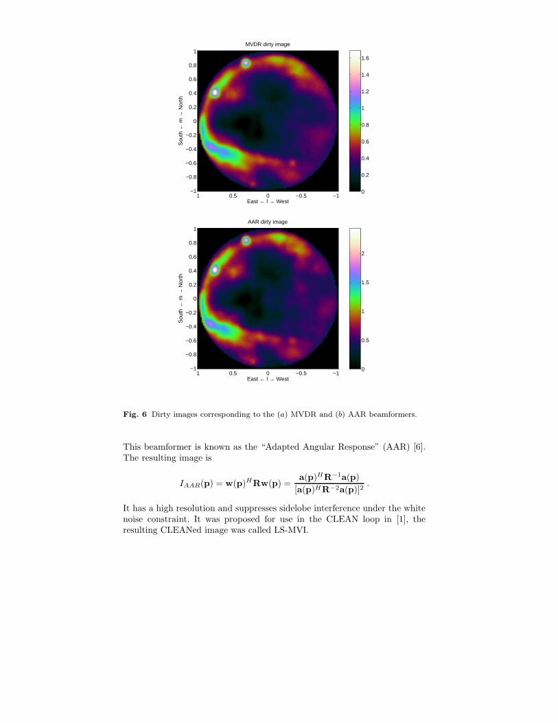
Fig. 6 Dirty images corresponding to the (a) MVDR and (b) AAR beamformers.

This beamformer is known as the “Adapted Angular Response” (AAR) [6].The resulting image is

IAAR(p) = w(p)HRw(p) =a(p)HR−1a(p)

[a(p)HR−2a(p)]2.

It has a high resolution and suppresses sidelobe interference under the whitenoise constraint. It was proposed for use in the CLEAN loop in [1], theresulting CLEANed image was called LS-MVI.

Example MVDR and AAR dirty images using the same LOFAR station asbefore are shown in figure 6. At first sight, the performance of these imagesis quite similar to that of the original dirty image in figure 5. There maybe situations where the differences are more pronounced (see [1] for exam-ples), e.g., the resolution for closely spaced point sources is expected to besignificantly improved.

5 Least Squares imaging

In the previous section, we discussed various algorithms based on the CLEANalgorithm. This algorithm uses a successive approximation of the dirty imageusing a point source model. In this section, we take a model-based approach.The imaging problem is formulated as a parametric estimation problem wherecertain parameters (source locations, powers, noise variance) are unknownand need to be estimated. Although we start from a Maximum Likelihoodformulation, we will quickly arrive at a more feasible Least Squares approach.The discussion follows to some extent [31], which is a general array processingapproach to a very similar problem and can be read for further details.

5.1 Matrix formulation of the data model

Let us start again from the data model (8). For simplicity, we consider onlya single frequency bin and STI interval, but all results can be generalizedstraightforwardly. The model for the signals arriving at the antenna array isthus

x(n) = As(n) + n(n)

and the covariance of x is (viz. (12))

R = AΣsAH + Σn .

We have available a sample covariance matrix

R =1

N

∑

n

x(n)x(n)H

which serves as the input data for the imaging step. Let us now vectorize thisdata model by defining

r = vec(R) , r = vec(R)

where r has the data model (using (4))

r = (A ◦A)σs + vec(Σn) .

If Σn is diagonal, we can write vec(Σn) = (I ◦ I)σn, where σn is a vectorcontaining the diagonal entries of Σn. Define Ms = A ◦ A and Mn = I ◦ I.Then

r = Msσs + Mnσn = [Ms Mn]

[

σs

σn

]

= Mσ .

In this formulation, several modifications can be introduced. E.g., a nondi-agonal noise covariance matrix Σn will lead to a more general Mn, and ifΣn = σ2

nI, we have Mn = vec(I) and σn = σ2n. Some other options are

discussed in [31].We can further write

r = r + w = Mσ + w , (23)

where r is the available “measurement data”, r is its mean (expected value),and w is zero mean additive noise. It is not hard to derive that (for Gaussiansignals) the covariance of this noise is [31]

Cw = E(r − r)(r − r)H =1

N(R ⊗R)

where N is the number of samples on which R is based. We have thus writtenour original data model on x as a similar data model on r. Many estimationtechniques from the literature that are usually applied to data models for x

can be applied to the data model for r. Furthermore, it is straightforward toextend this vectorized formulation to include multiple snapshots over timeand frequency to increase the amount of measurement data and thus to im-prove the imaging result: Simply stack the covariance data in r and includethe model structure in M; note that σ remains unchanged.

The unknown parameters in the data model are, first of all, the powers σ.These appear linear in the model. Regarding the positions of the sources, wecan consider two cases:

1. We consider a point source model with a “small” number of sources. Inthat case, A = A(θ) and M = M(θ), where θ is some parametrizationof the unknown locations of the sources (the position vectors pq for eachsource). These enter in a nonlinear way into the model M(θ). The imageI(p) is constructed following (14), usually convolved with a synthetic beamBsynth(p) to make the image look nicer.

2. Alternatively, we consider a model where for each pixel in the image, weassume a corresponding point source: the source positions pq directly cor-respond to the pixels in the image. This can lead to a large number ofsources. With the locations of the pixels predetermined, M is a prioriknown and not a function of θ, but M will have many columns (one for

each pixel-source). The image I(p) has a one-to-one relation to the sourcepower vector σs, we can thus regard σs as the image in this case.

We need to pose several requirements on M or M(θ) to ensure identifia-bility. First of all, in the first case we must have M(θ) = M(θ′) → θ = θ

′,otherwise we cannot uniquely find θ from M. Furthermore, for both cases wewill require that M is a tall matrix (more rows than columns) and has fullcolumn rank, so that it has a left inverse (this will allow to estimate σ). Thisputs a limit on the number of sources in the image (number of columns of M)in relation to the number of observations (rows). If more snapshots (STIs)and/or multiple frequencies are available, as is the case in practice, then M

will become taller, and more sources can be estimated thus increasing theresolution. If M is not tall, then there are some ways to generalize this, e.g.via the context of compressive sampling where we can have M wide as longas σ is sparse [43], which we will briefly discuss in subsection 5.6.

For the moment, we will continue with the second formulation: one sourceper pixel, fewer pixels than available correlation data.

5.2 Matrix formulation of imaging via beamforming

Let us now again interprete the “beamforming image” (20) as a linear trans-formation on the covariance data r. We can stack all image values I(p) overall pixels p into a single vector i, and similarly, we can collect the weightsw(p) over all pixels into a single matrix W = [w(p1), w(p2), · · · ]. From(3), we know that wHRw = (w ⊗w)Hvec(R), so that we can write

iBF = (W ◦W)H r . (24)

We saw before that the dirty image is obtained if we use the matched filter.In this case, we have W = 1

J A, where A contains the array response vectorsa(p) for every pixel p of interest. In this case, the image is

iD =1

J2(A ◦A)H r =

1

J2MH

s r . (25)

The expected value of the image is obtained by using r = Mσ:

iD =1

J2MH

s Mσ =1

J2(MH

s Ms)σs +1

J2(MH

s Mn)σn .

The quality or “performance” of the image, or how close iD is to iD, is relatedto its covariance,

cov(iD) = E{(iD − iD)(iD − iD)H} =1

J4MH

s CwMs

where Cw = 1N (R⊗R) is the covariance of the noise on the covariance data.

Since usually the astronomical sources are much weaker than the noise (oftenat least by a factor 100), we can approximate R ≈ Σn. If the noise is spatially

white, Σn = σ2nI, we obtain for the covariance of iD

cov(iD) ≈ σ4n

J4NMH

s Ms .

The variance in the image is given by the diagonal of this expression. Fromthis and the structure of Ms = (A ◦ A) and the structure of A, we can seethat the variance on each pixel in the dirty image is constant, σ4

n/(J2N), butthat the noise on the image is correlated, possibly leading to visible structuresin the image. This is a general phenomenon.

Similar equations can be derived for the MVDR image and the AAR image.

5.3 Weighted Least Squares imaging

At this point, the deconvolution problem can be formulated as a maximumlikelihood (ML) estimation problem, and solving this problem should pro-vide a statistically efficient estimate of the parameters. Since all signals areassumed to be i.i.d. Gaussian signals, the derivation is standard and the MLestimates are obtained by minimizing the negative log-likelihood function [31]

{σ, θ} = argminσ,θ

(

ln |R(σ, θ)| + tr(

R−1(σ, θ)R))

. (26)

where | · | denotes the determinant. R(σ, θ) is the model, i.e., vec(R(σ, θ)) =r = M(θ)σ.

In this subsection, we will consider the overparametrized case, where eachpixel in the image corresponds to a source. In this case, M is a priori known,the model is linear, and the ML problem reduces to a Weighted Least Squares(WLS) problem to match r to the model r:

σ = arg minσ

‖C−1/2w (r − r)‖2

2 = argminσ

(r −Mσ)HC−1w (r −Mσ) (27)

where we fit the “data” r to the model r = Mσ. The correct weighting is theinverse of the covariance of the residual, w = r− r, i.e., the noise covariancematrix Cw = 1

N (R⊗R). For this, we may also use the estimate Cw obtained

by using R instead of R. Using the assumption that the astronomical sourcesare much weaker than the noise we could contemplate to use R ≈ Σn for theweighting. If the noise is spatially white, Σn = σ2

nI, the weighting can theneven be omitted.

The solution of (27) is obtained by applying the pseudo-inverse,

East ← l → West

Sou

th ←

m →

Nor

th

WLS image estimate

Cas A

Cyg Aloop III

NPSVir A

Sun

−0.500.5

−0.8

−0.6

−0.4

−0.2

0

0.2

0.4

0.6

0.8

0

0.2

0.4

0.6

0.8

1

1.2

1.4

Fig. 7 Image corresponding to the WLS formulation (28).

σ = [C−1/2w M]†C−1/2

w r = (MHC−1w M)−1MHC−1

w r =: M−1d σd (28)

whereMd := MHC−1

w M , σd := MHC−1w r .

Here, we can consider the term σd = MHC−1w r as a “dirty image”: it is

comparable to (25), although we have introduced a weighting by C−1w and

estimate the noise covariance parameters σn as well as the source powersin σs (the actual image). The factor 1/J2 in (25) can be seen as a crudeapproximation of M−1

d .Figure 7 shows an example WLS image for the same LOFAR data set as

before. The resolution (number of pixels) in this image is kept limited (about1000) for reasons discussed below.

The term M−1d = (MHC−1

w M)−1 is a deconvolution operation. This inver-sion can only be carried out if the deconvolution matrix Md = MHC−1

w M isnot rank deficient. This requires at least that M is a tall matrix (“less pixelsthan observations” in case we take one source per pixel). Thus, high resolu-tion WLS imaging is only possible if a limited number of sources is present.The condition number of Md, i.e., the ratio of the largest to the smallesteigenvalue of Md, gives important information on our ability to compute itsinverse: LS theory tells us that the noise on σd could, in the worst case, bemagnified by this factor. The optimal (smallest) condition number of anymatrix is 1, which is achieved if Md is a scaling of the identity matrix, or

if the columns of C−1/2w M are all orthogonal to each other. If the size of M

becomes less tall, then the condition number of Md becomes larger (worse),

East ← l → West

Sou

th ←

m →

Nor

th

KLT image

−1−0.500.51−1

−0.8

−0.6

−0.4

−0.2

0

0.2

0.4

0.6

0.8

1

−0.05

0

0.05

0.1

0.15

Fig. 8 Image corresponding to the KLT solution (29).

and once it is a wide matrix, M is singular and the condition number will beinfinite. Thus, we have a trade-off between the resolution (number of pixelsin the image) and the noise enhancement.

The definition of Md shows that it is not data dependent, and it canbe precomputed for a given telescope configuration and observation interval.It is thus possible to explore this trade-off beforehand. To avoid numericalinstabilities (noise enhancement), we would usually compute a regularizedinverse or pseudo-inverse of this matrix, e.g., by first computing the eigenvaluedecomposition

Md = UΛUH

where U contains the (orthonormal) eigenvectors and Λ is a diagonal matrixcontaining the eigenvalues, sorted from large to small. Given a threshold εon the eigenvalues, we can define Λ to be a diagonal matrix containing onlythe eigenvalues larger than ε, and U a matrix containing the correspondingeigenvectors. The ε-threshold pseudo-inverse is then given by

M†d := UΛ

−1UH

and the resulting image is

σ = UΛ−1

UHσd . (29)

This can be called the “Karhunen-Loeve” image, as the rank reduction isrelated to the Karhunen-Loeve transform (KLT). It corresponds to selecting

an optimal (Least Squares) set of basis vectors on which to project a certaindata set, here σd.

An example KLT image is shown in figure 8. In this image, the number ofpixels is much larger than before in figure 7 (about 9000), but the rank of thematrix Md is truncated at 1/200 times the largest eigenvalue, leaving about1300 out of 9000 image components. The result is not quite satisfactory: thetruncation to a reduced basis results in annoying ripple artifacts in the image.

Computing the eigenvalue decomposition for large matrices is complex. Acomputationally simpler alternative is to compute a regularized inverse ofMd, i.e., to take the inverse of Md + εI. This should yield similar (althoughnot identical) results.

If we use the alternative sky model where we assume a point source modelwith a “small” number of sources (M = M(θ)), then the conditioning ofMd, and thus the performance of the deconvolution, is directly related tothis number of sources.

The perfomance of the method is assessed by looking at the covariance ofthe resulting image (plus noise parameters) σ in (28). It is given by

Cσ = (MHC−1w M)−1MHC−1

w (Cw)C−1w M(MHC−1

w M)−1

= (MHC−1w M)−1 = M−1

d .

This again shows that the performance of the imaging method follows directlyfrom the conditioning of the deconvolution matrix Md. If Md is sufficientlywell conditioned, the noise on the image is limited, otherwise it may be large.The formulation also shows that the pixels in the image are correlated (Md

is in general not diagonal), as we obtained before for the dirty image.

Similarly, if we use the pseudo-inverse M†d = UΛ

−1UH for the deconvolu-

tion, then we obtain Cσ = M†d. In this case, the noise enhancement depends

on the chosen threshold ε. Also, the rank of Cσ depends on this threshold,and since it is not full rank, the number of independent components (sources)in the image is smaller than the number of shown pixels: the rank reductiondefines a form of interpolation.

Using a rank truncation for radio astronomy imaging was already sug-gested in [7]. Unfortunately, if the number of pixels is large, this techniqueby itself is not sufficient to obtain good images, e.g., the resulting pixelsmay not all be positive, which is unplausible for an intensity image. Thus,the overparametrized case requires additional constraints; some options arediscussed in subsection 5.6.

5.4 Estimating the position of the sources

Let us now consider the use of the alternative formulation, where we writeA = A(θ) and M = M(θ), where θ captures the positions of the limited

number of sources in the image. In this case, we have to estimate both σ andθ. If we start again from the ML formulation (26), it does not seem feasibleto solve this minimization problem in closed form. However, we can againresort to the WLS covariance matching problem and solve instead

{σ, θ} = argminσ,θ

‖C−1/2w (r − r(σ, θ))‖2

= argminσ,θ

(r −M(θ)σ)HC−1w (r −M(θ)σ) . (30)

It is known that the resulting estimates are, for a large number of samples,equivalent to ML estimates and therefore asymptotically efficient [31].

The WLS problem is separable: suppose that the optimal θ is known, sothat M = M(θ) is known, then the corresponding σ will satisfy the solutionwhich we found earlier:

σ = (MHC−1w M)−1MHC−1

w r .

Substituting this solution back into the problem, we obtain

θ = argminθ

rH [I−M(θ)(M(θ)HC−1w M(θ))−1M(θ)HC−1

w ]H ·

· C−1w · (I −M(θ)(M(θ)HC−1

w M(θ))−1M(θ)HC−1w ]r

= argminθ

rHC−1/2w (I − Π(θ))C−1/2

w r

= argmaxθ

rHC−1/2w Π(θ)C−1/2

w r

where Π(θ) = C−1/2w M(θ)

(

M(θ)HC−1w M(θ)

)−1M(θ)HC

−1/2w .

Π(θ) is an orthogonal projection: Π2 = Π, Π

H = Π . The projection is

onto the column span of M′(θ) := C−1/2w M(θ). The estimation of the source

positions θ is nonlinear. It could be obtained iteratively using a Newtoniteration (cf. [31]). The sources can also be estimated sequentially [31], whichprovides an alternative to the CLEAN algorithm.

5.5 Two-step WLS solution

In the previous formulation (28), we estimated σ, which contains both thesource powers and the noise powers. However, the image is related only tothe source powers, σs. We can write more explicitly how these are estimated.

The optimization problem is again separable: given the optimal σs, the“known” part of the LS problem (27) is r − Msσs, and the correspondingestimate for σn is

σn = (MHn C−1

w Mn)−1MnC−1w (r −Msσs) . (31)

Plugging this solution back into the LS problem, we can first rewrite

C−1/2w (r −Msσs −Mnσn)

= [C−1/2w −C−1/2

w Mn(MHn C−1

w Mn)−1MnC−1w ]r −

−[C−1/2w −C−1/2

w Mn(MHn C−1

w Mn)−1MnC−1w ]Msσs

= P⊥C−1/2w (r −Msσs)

where

P⊥ = I −P , P = C−1/2w Mn(MH

n C−1w Mn)−1MnC−1/2

w .

Similar to Π , we can show that P is an orthogonal projection. Hence, alsoP⊥ = I − P is an orthogonal projection, onto the complement of the range

of C−1/2w Mn, i.e., the weighted range of the noise matrix. If Σn is diagonal,

this is equivalent to “projecting out the diagonal”, thus omitting these entriesin the WLS fitting. It is interesting to note that, in current telescopes, theautocorrelations (main diagonal of R) are usually not estimated. That fits invery well with this scheme, as the projection would project them out anyway!

The resulting “compressed” WLS problem is

σs = arg minσs

‖C−1/2s (r −Msσs)‖2

whereC−1

s := C−1/2w P⊥C−1/2

w .

(This is with some abuse of notation: Cs is singular due to the projection,hence not invertible. However, we will only need C−1

s , and will use the abovedefinition for it.) The solution σs will be exactly the same as in the originalWLS problem (27), but now it is obtained in two steps: first σs and then, ifrequired, σn via (31).

As the expression for the compressed problem is very similar to the originalWLS problem, we obtain similar results: the solution is

σs = (MHs C−1

s Ms)−1MH

s C−1s r

which can also be written as

σs = M−1ds σds , Mds = MH

s C−1s Ms , σds = MH

s C−1s r .

Mds is the deconvolution matrix, and σds is the WLS dirty image. Thistime, the dirty image is really a (vectorized) image, whereas in the previousdiscussion, the vector σd had an image component and a noise component.

The covariance of the image estimate σs is, using C−1s CwC−1

s = C−1s ,

Cσs= (MH

s C−1s Ms)

−1MHs C−1

s (Cw)C−1s Ms(M

Hs C−1

s Ms)−1 = M−1

ds .

Thus, we obtain quite similar results as before when we estimated σ, but nowdirectly related to the image σs, with the noise part σn “projected out”.

5.6 Imaging using sparse reconstruction techniques

Compressive sampling/sensing (CS) is a “new” topic, currently drawing wideattention. It is connected to random sampling, and as such, it has been usedin radio astronomy for a long time. In its basic formulation, we connect backto the measurement equation (23), or r = Mσ + w, and we consider the“overparametrized” formulation where each pixel in the image correspondsto a potential source in σ, whereas M is known. If the image is large, then thedeconvolution problem (inversion of M) is ill conditioned. A direct inversionusing (Weighted) Least Squares will give rise to unacceptable noise enhance-ment. We resorted to regularization by the KLT, which essentially projectsthe true image onto the selected basis, giving rise to artefacts. Without noise,any component orthogonal to the projection space can be added to the im-age without changing the modeling error: the image that fits the data is notunique. Additional constraints are needed. Examples are:

1. Sparsity of the solution vector, typically obtained by using an `1 norm(sum of absolute values), resulting in convex optimization problems like[21, 43]

minσ

‖σ‖1 subject to ‖r −Mσ‖22 ≤ ε

or the equivalentminσ

‖r−Mσ‖22 + λ‖σ‖1

These are versions of the Basis Pursuit problem. Like the KLT, the resultsdepend on the chosen noise threshold ε (or regularization parameter λ).The sparsity assumption poses that the sky is mostly empty. Although ithas already long been suspected that CLEAN is related to `1-optimization[27] (in fact, it is now recognized as a Matching Pursuit algorithm [25]),CS theory states the general conditions under which this assumption islikely to recover the true image [21, 43]. Extensions are needed in case ofextended emissions [23].

2. Requiring the resulting image to be non-negative. This is physically plau-sible, and to some extent already covered by CLEAN [27]. It is an explicitcondition in a Non-Negative Least Squares (NNLS) formulation [7], whichsearches for a Least Squares fit while requiring that the solution σ has allentries σi ≥ 0. This turns out to be a strong constraint, readily incorpo-rated into other formulations (e.g., CLEAN, MEM, and `1-optimization).

Some experimental results using these algorithms are shown in [23, 35].

6 Calibration

6.1 Non-ideal measurements

The previous section showed that there are many options to make an imagefrom radio interferometer data. However, there are in fact several effects thatmake matters more complicated.

Instrumental effects

So far we ignored the beam shape of the individual elements (antennas ordishes) of the array. In fact, any antenna has its own directional response,b(p). This function is called the primary beam (to distinguish it from thedirty beam that results from beamforming during the synthesis operation).It is generally assumed that the primary beam is equal for all elements inthe array. With Q point sources, we will collect the resulting samples of theprimary beam into a vector b = [b(p1), · · · , b(pQ)]T . These coefficients areseen as gains that (squared) will multiply the source powers σ2

q . The generalshape of the primary beam b(p) is known from electromagnetic modelingduring the design of the telescope. If this is not sufficiently accurate, then ithas to be calibrated.

Initially the direction independent electronic gains and phases of the re-ceiver chain of each element in the array are unknown and have to be esti-mated. They are generally different from element to element. We thus havean unknown vector g (size J × 1) with complex entries that each multiplythe output signal of each telescope.

Also the noise powers of each element are unknown and generally unequalto each other. We will still assume that the noise is independent from elementto element. We can thus model the noise covariance matrix by an (unknown)diagonal Σn.

The modified data model that captures the above effects and replaces (12)is

R = (ΓAB)Σs(BHAH

ΓH) + Σn (32)

where Γ = diag(g) is a diagonal with unknown receiver complex gains, andB = diag(b) contains the samples of the primary beam. Usually, Γ and B

are considered to vary only slowly with time m and frequency k, so that wecan combine multiple covariance matrices Rm,k with the same Γ and B.

Propagation effects

Ionospheric and tropospheric turbulence cause time-varying refraction anddiffraction, which has a profound effect on the propagation of radio waves. In

geometric delays

(time varying)phase screen

ionosphere

beamformersstation

xJ(t)x1(t)

Fig. 9 A radio interferometer where stations consisting of phased array elementsreplace telescope dishes. The ionosphere adds phase delays to the signal paths. If theionospheric electron density has the form of a wedge, it will simply shift the apparentpositions of all sources.

the simplest case, the ionosphere is modeled as a thin layer at some height(say 100 km) above the Earth, causing delays that can be represented as phaseshifts. At the low frequencies used for LOFAR, this effect is more pronounced.Generally it is first assumed that the ionosphere is “constant” over about 10km and about 10 s. A better model is to model the ionospheric delay asa “wedge”, a linear function of the distance between piercing points (theintersection of the direction vectors pq with the ionospheric phase screen).As illustrated in figure 9, this modifies the geometric delays, leading to ashift in the apparent position of the sources. For larger distances, higher-order functions are needed to model the spatial behavior of the ionosphere,and if left uncorrected, the resulting image distortions are comparable to thedistortions one sees when looking at lights at the bottom of a swimming pool.

Previously, we described that the array response matrix A is really afunction of the source direction vectors pq, and we wrote A(θ) where thevector θ is a suitable parametrization of the pq (typically two direction cosinesper source). If a linear model for the ionospheric disturbance is sufficient, thenit is sufficient to replace A(θ) by A(θ′), where θ

′ differs from θ due to theshift in apparent direction of each source.

The modified data model that captures the above effects is thus

R = (ΓA(θ′)B)Σs(BHA(θ′)H

ΓH) + Σn . (33)

If we wish to be very general, we can write

R = (G �A(θ))Σs(G �A(θ))H + Σn (34)

where � indicates an entrywise multiplication of two matrices (Schur-Hadamardproduct). Here, G is a full matrix that captures all non-linear measurementeffects. Equation (32) is recovered if we write G = gbH (i.e., a rank-1 ma-trix), and equation (33) if we write G = gbH � A′, where A′ is a matrixconsisting of phase corrections such that A(θ′) = A(θ) �A′.

Calibration is the process of identifying the unknown parameters in G, andsubsequently correcting for G during the imaging step. The model (34) inits generality is not identifiable unless we make assumptions on the structureof G (in the form of a suitable parametrization) and describe how it varieswith time and frequency, e.g., in the form of (stochastic) models for thesevariations.

In practice, calibration is an integral part of the imaging step, and nota separate phase. In the next subsection, we will first describe how modelsof the form (32) or (33) can be identified. This step will serve as a steppingstone in the identification of a more general G.

6.2 Calibration algorithms

Estimating the element gains and directional responses

Let us assume a model of the form (32), where there are Q dominant calibra-tion sources within the field of view. For these sources, we assume that theirpositions and source powers are known with sufficient accuracy from tables,i.e., we assume that A and Σs are known. We can then write (32) as

R = ΓAΣAHΓ

H + Σn (35)

where Σ = BΣsB is a diagonal with apparent source powers. With B un-known, Σ is unknown, but estimating Σ is precisely the problem we studiedbefore when we discussed imaging. Thus, once we have estimated Σ andknow Σs, we can easily estimate the directional gains B. The problem thusreduces to estimate the diagonal matrices Γ , Σ and Σn from a model of theform (35).

For some cases, e.g., arrays where the elements are traditional telescopedishes, the field of view is quite narrow (degrees) and we may assume thatthere is only a single calibrator source in the observation. Then Σ = σ2 is ascalar and the problem reduces to

R = gσ2gH + Σn

and since g is unknown, we could even absorb the unknown σ in g (it isnot separately identifiable). The structure of R is a rank-1 matrix gσ2gH

plus a diagonal Σn. This is recognized as a “rank-1 factor analysis” model inmultivariate analysis theory [26, 18]. Given R, we can solve for g and Σn inseveral ways [4, 5, 48]. For example, any submatrix away from the diagonalis only dependent on g and is rank 1. This allows direct estimation of g.This property is related to the gain and phase closure relations often used inthe radio astronomy literature for calibration (in particular, these relationsexpress that the determinant of any 2 × 2 submatrix away from the maindiagonal will be zero, which is the same as saying that this submatrix is rank1).

In general, there are more calibrator sources (Q) in the field of view, andwe have to solve (35). We resort to an Alternating Least Squares approach. IfΓ would be known, then we can correct R for it, so that we have precisely thesame problem as we considered before, (27), and we can solve for Σ and Σn

using the techniques discussed in section 5.3. Alternatively, with Σ known,we can say we know a reference model R0 = AΣAH , and the problem is toidentify the element gains Γ = diag(g) from a model of the form

R = ΓR0ΓH + Σn

or, after applying the vec(·)-operation,

vec(R) = diag(vec(R0))(g ⊗ g) + vec(Σn) .

This leads to the Least Squares problem

g = argming

‖vec(R− Σn) − diag(vec(R0))(g ⊗ g)‖2 .

This problem cannot be solved in closed form. Alternatively, we can first solvean unstructured problem: define x = g ⊗ g and solve

x = diag(vec(R0))−1vec(R− Σn)

or equivalently, if we define X = ggH ,

X = (R − Σn) �R0.

where � denotes an entrywise matrix division. After estimating the unstruc-tured X, we enforce the rank-1 structure X = ggH , via a rank-1 approxi-mation, and find an estimate for g. The pointwise division can lead to noiseenhancement; this is remediated by only using the result as an initial estimatefor a Gauss-Newton iteration [13] or by formulating a weighted least squaresproblem instead [45, 48].

With g known, we can again estimate Σ and Σn, and make an iteration.Overall we then obtain an alternating least squares solution. A more optimalsolution can be found by solving the overall problem (35) as a covariancematching problem with a suitable parametrization, and the more generalalgorithms in [31] lead to an asymptotically unbiased and statistically efficientsolution.

The resulting algorithms are related to the classical self-calibration (Self-Cal) algorithm [10, 32] widely used in the radio astronomy literature, inparticular for a single calibrator source. In that algorithm, R0 is a referencemodel, obtained from the best known map at that point in the iteration. Inthe SelfCal iteration, the telescope gains are estimated, the corrections onR are made, the next best image is constructed leading to a new referencemodel R0, etc.

Estimating the ionospheric perturbation

The more general calibration problem (33) follows from (32) by writing A =A(θ′) where θ

′ are the apparent source locations. This problem can be easilysolved in quite the same way: in the alternating least squares problem wesolve for g, θ

′, σs and σn in turn, keeping the other parameters fixed at theirprevious estimates. After that, we can relate the apparent source locationsto the (known) locations of the calibrator sources θ.

The resulting phase corrections A′ to relate A(θ′) to A(θ) via A(θ′) =A(θ)�A′ gives us an estimate of the ionospheric phase screen in the directionof each source. These “samples” can then be interpolated to obtain a phasescreen model for the entire field of view. This method is limited to the regimewhere the phase screen can be modeled as a linear gradient over the array.An implementation of this algorithm is called Field-Based Calibration [11].

Other techniques are based on “peeling” [28]. In this method of succes-sive estimation and subtraction calibration, parameters are obtained for thebrightest source in the field. The source is then removed from the data, andthe process is repeated for the next brightest source. This leads to a collectionof samples of the ionosphere, to which a model phase screen can be fitted.

Estimating the general model

In the more general case (34), viz.

R = (G �A)Σs(G�A)H + Σn ,

we have an unknown full matrix G. We assume A and Σs known. Since A

pointwise multiplies G and G is unknown, we might as well omit A fromthe equations without loss of generality. For the same reason also Σs can be

omitted. This leads to a problem of the form

R = GGH + Σn ,

where G : J ×Q and Σn (diagonal) are unknown. This problem is known asa rank-Q factor analysis problem. For reasonably small Q, as compared tothe size J of R, the factor G can be solved for, again using algorithms forcovariance matching such as in [31]. We discuss this problem in more detailin section 7.

It is important to note that G can be identified only up to a unitary factorV at the right: G′ = GV would also be a solution. This factor makes thegains unidentifiable unless we introduce more structure to the problem.

To make matters worse, note that this problem is used to fine-tune earliercoarser models (33). At this level of accuracy, the number of dominant sourcesQ is often not small anymore, making G not identifiable.

As discussed in [30] and studied in more detail in [39], more structureneeds to be introduced to be able to solve the problem. Typically, what helpsis to consider the problem for a complete observation (rather than for a singlesnapshot R) where we have many different frequencies fk and time intervalsm. The directional response matrix Am,k varies with m and k in a known way,and the instrumental gains g and b are relatively constant. The remainingpart of G = gbH�A′ is due to the ionospheric perturbations, and models canbe introduced to describe its fluctuation over time, frequency, and space usingsome low order polynomials. We can also introduce stochastic knowledge thatdescribe a correlation of parameters over time and space.

New instruments such as LOFAR and SKA will only reach their full poten-tial if this general calibration problem is solved. For LOFAR, a complete cali-bration method that incorporates many of the above techniques was recentlyproposed in [16]. In general, calibration and imaging need to be consideredin unison, leading to many potential directions, approaches, and solutions.This promises to be a rich research area in years to come.

7 Factor analysis

7.1 Introduction

Many array signal processing algorithms are at some point based on the eigen-value decomposition, which is used e.g., to make a distinction between the“signal subspace” and the “noise subspace”. By using orthogonal projections,part of the noise is projected out and only the signal subspace remains. Thiscan then be used for applications such as high-resolution direction-of-arrivalestimation, blind source separation, etc. In these applications, it is commonly

assumed that the noise is spatially white. However, this is valid only aftersuitable calibration.

Factor analysis considers covariance data models where the noise is un-correlated but has unknown powers at each sensor, i.e., the noise covariancematrix is an arbitrary diagonal with positive real entries. In these cases thefamiliar eigenvalue decomposition (EVD) has to be replaced by a more gen-eral “Factor Analysis” decomposition (FAD), which then reveals all relevantinformation. It is a very relevant model for the early stages of data processingin radio astronomy, because at that point the instrument is not yet calibratedand the noise powers on the various antennas may be quite different. We sawtwo examples in section 6.

As it turns out, this problem has been studied in the psychometrics, bio-metrics and statistics literature since the 1930s (but usually for real-valuedmatrices) [18, 26]. The problem has received much less attention in the signalprocessing literature. In this section, we briefly describe the FAD and somealgorithms for computing it.

7.2 Problem formulation

Assume as before that we have a set of Q narrow-band Gaussian signalsimpinging on an array of J sensors. The received signal can be described incomplex envelope form by

x(n) =

Q∑

q=1

aqsq(n) + n(n) = As(n) + n(k) (36)

where A = [a1, · · · , aQ] contains the array response vectors. In this model,A is unknown, and the array response vectors are unstructured, i.e., we donot consider a directional model for them. The source vector s(n) and noisevector n(n) are considered i.i.d. Gaussian, i.e., the corresponding covariancematrices are diagonal. Without loss of generality, we can scale the sourcesignals such that the source covariance matrix Σs is identity.

The data covariance matrix thus has the form

R = AAH + D (37)

where we assume Q < J so that AAH is rank deficient. Many signal process-ing algorithms are based on computing an eigenvalue decomposition of R asR = UΛUH , where U is unitary and Λ is a diagonal matrix containing theeigenvalues in descending order.

If D = 0 (no noise), then R has rank Q and the eigenvalue decompositionspecializes to

R = UΛ0UH = [Us Un]

[

Λs

0

] [

UHs

UHn

]

where Λs contains the Q nonzero eigenvalues and Us the correspondingeigenvectors. The range of Us is called the signal subspace, its orthogonalcomplement Un the noise subspace.

For spatially white noise, D = σ2I, we can write D = σ2UUH , and theeigenvalue decomposition becomes

R = UΛUH = U(Λ0 + σ2I)UH = [Us Un]

[

Λs + σ2I

σ2I

] [

UHs

UHn

]

.

Hence, all eigenvalues are raised by σ2, but the eigenvectors are unchanged.Algorithms based on Us can thus proceed as if there was no noise, thusleading to the use of the EVD and related subspace estimation algorithms inmany array signal processing applications.

If the noise is not uniform, then D is an unknown diagonal matrix, and theEVD does not reveal the signal subspace Us. The objective of factor analysisis, for given R, to identify A and D, as well as the factor dimension Q. Thiscan be seen as an extension of the eigenvalue decomposition, to be used ifthe noise covariance is a diagonal.

It is clear that for an arbitrary Hermitian matrix R, this factorization canexist in its exact form only for Q ≥ J , in which case we can set D = 0, orany other value, which makes the factorization useless. Hence, for a noise-perturbed matrix, we wish to detect the smallest Q which gives a “reasonablefit”, and we will assume that Q < J is sufficiently small so that uniquedecompositions exist.

Furthermore, we cannot estimate A uniquely, since A can be replaced byAV for an arbitrary unitary matrix V. If we denote AAH = UsΛsU

Hs , it is

clear that we can only estimate the column span of A, i.e., ran(A) = ran(Us),as well as the “signal eigenvalues” Λs.

Suppose we have estimated D, then we can whiten R:

R := D−1/2RD−1/2 = (D−1/2A)(AHD−1/2) + I .

At this point, we can introduce the usual eigenvalue decomposition of R:

R = UΛUH

and identify D−1/2AV = U, or A = D1/2UVH , where V is an arbitraryunitary factor. If we choose V = I, we obtain AHD−1A = Λ is diago-nal, which is a constraint that is sometimes used to obtain a more uniqueparametrization of A. Note that A is not yet quite unique, because in thecomplex case each column of A can be scaled by an arbitrary complex phase,and the columns may be reordered as well. However, the point is that onceD is known, we are back on familiar grounds.

Regarding identifiability, we generally require to have more “equations”than “unknowns”. Here, the number of available equations is equal to thenumber of (real) parameters in R, which is J (real) entries on the main diag-onal and J(J − 1) parameters for the off-diagonal (complex) entries, takinginto account Hermitian symmetry. The number of unknowns is 2JQ (real)parameters for A, and J parameters for D, minus the number of constraintsto make A unique. Taking the constraint that AHD−1A is diagonal givesQ2 −Q constraints on the parameters of A, and further setting the first rowof A to be real gives another Q constraints. In total we have for the numberof equations minus the number of unknowns

s = J + J(J − 1) − (2JQ + J − (Q2 − Q + Q)) = (J − Q)2 − J .

Requiring s > 0 leads to the condition Q < J −√

J . This is an upper boundon the factor rank.

In Factor Analysis, there are two problems:

1. Detection: given R, estimate Q. The hypothesis that the factor rank is qis denoted by Hq .

2. Identification: given R and Q, estimate D and A, or Λs and Us.

We consider the latter problem first.

7.3 Computing the Factor Analysis decomposition

Assume we know Q. Let θ be a minimal parametrization of (A,D), dependenton Q, such that R(θ) = AAH +D. If we start from a likelihood perspective,we obtain after standard derivations that the maximum likelihood estimateof R is obtained by finding the model parameters θ such that

θ = argminθ

N(

ln |R(θ)| + tr(R(θ)−1R))

.

where R = 1N

∑Nn=1 x(n)x(n)H is the sample covariance matrix. This is

exactly the same problem as we saw before in (26), and we can follow thesame solution strategy.

In particular, we can use the result from [31] that the ML problem isasymptotically (large N) equivalent to the Weighted Least Squares problem

θ = argminθ

‖C−1/2w (r − r(θ))‖2 = arg min

θ

(r − r(θ))HC−1w (r − r(θ)) (38)

where as before r = vec(R), r = vec(R), and the weighting matrix Cw is thecovariance of r, i.e., Cw = (1/N)(R⊗R). This is precisely in context of [31],

and we can use the algorithms proposed there: Gauss-Newton iterations, thescoring algorithm or sequential estimation algorithms.

It is also possible to propose an alternating least squares approach. Givenan estimate for D, then, as mentioned above, we can whiten R by D, doan eigenvalue decomposition on R = D−1/2RD−1/2, and estimate A of sizeJ×Q, taking into account some suitable constraints to make A unique. For A

known, the optimal D in turn is given by diag(R−AAH). Given a reasonableinitial point (e.g., D(0) = diag(R)), we can easily alternate between these twosolutions. Convergence is to a local optimum and may be very slow.

An alternative approach was recently proposed in [36]. The ML cost func-tion is shown to be equivalent to the Kullback-Leibler norm as often used ininformation theory, and a suitable algorithm is the Expectation Maximiza-tion (EM) algorithm. This is an iterative estimation algorithm which is shownin [36] to reduce, for current estimates (Ak ,Dk), to

Rk := AkAHk + Dk

Φk := I −AHk R−1

k Ak + AHk R−1

k RR−1k Ak

Ak+1 := RR−1k AkΦ

−1k

Dk+1 := diag(R −Ak+1AHk R−1

k R) .

As any EM algorithm, it will converge to a local optimum, where convergenceis guaranteed and typically reasonably fast.

7.4 Rank detection

The detection problem is to estimate the factor rank Q. The largest permis-sible value of Q is that for which the number of unknown (real) parameterss = (J −Q)2−J ≥ 0, or Q ≤ J −

√J . For larger Q, there is no identifiability

of A and D: any sample covariance matrix R can be fitted.To find Q, we can define a collection of hypotheses

Hq : x(k) ∼ CN (0, Rq) q = 1, 2, · · · (39)

which are tested in turn against the null hypothesis

H′ : x(k) ∼ CN (0, R′) ,

where CN (0, R) denotes the zero-mean complex normal distribution withcovariance R, and Rq is the covariance matrix of the model with q interferers,

Rq = AAH + D , where A : J × q , D diagonal .

H′ corresponds to a default hypothesis of an arbitrary (unstructured) positivedefinite matrix R′.

The generalized likelihood ratio test (GLRT) [17] is applicable. In this test,we have to insert maximum likelihood estimates for each of the unknownparameters, under each of the hypotheses. For Hq , we can use the estimationtechniques from the previous subsection. For H′, the ML estimate R′ is equalto the sample covariance, R′ = R.

Under Hq , respectively H′, the log-likelihood is (dropping constants)

log(Lq) = −N log |R−1q | − Ntr(R−1

q R)

log(L′) = −N log |R−1| − Np .

The log-likelihood ratio is then

log(λ) := log(L′

Lq) = Ntr(R−1

q R) + N log |R−1q R| − Np . (40)

Here, λ = L′/Lq is the test statistic (likelihood ratio), and we will reject Hq

and accept H′ if λ > γ, where γ is a predetermined threshold. Typically, γis determined such that we obtain an acceptable “false-alarm” rate (i.e., theprobability that we accept H′ instead of Hq, while Hq is actually true). Toestablish γ, we need to know the statistics of λ under Hq .

Generalizing the results from the real-valued case [18, 26], we obtain thatfor moderately large N (say N > 50), the test statistic 2 log(λ) has approxi-mately a χ2

s distribution, where s is equal to “the number of free parameters”under Hq (the number of equations minus the number of unknowns). For thecomplex case, this number is s = (J − q)2 − J degrees of freedom.

In view of results of Box and Bartlett, a better fit of the distribution of2 log(λ) to a χ2

s distribution is obtained by replacing N in (40) by [18, 26]

N ′ = N − 1

6(2J + 11) − 2

3Q .

To detect Q, we start with q = 0, and apply the test for increasing valuesof q until it is accepted, or until s = (J − q)2 − J is negative. In that case,the hypothesis H′ is accepted, i.e., the given R is an unstructured covariancematrix. A disadvantage of this process is that the model parameters for eachq have to be estimated, which can become quite cumbersome if J is large.Also, as for any sequential hypothesis test, the actual false alarm rate thatis achieved is unknown, because the tests are not independent.

7.5 Application to interference cancellation

In the context of radio astronomy, factor analysis shows up in a numberof applications. We already mentioned calibration in section 6. Another ap-plication is interference cancellation. In general, this is a large topic withmany aspects. Here, we consider a simple case where we take short STIsand an uncalibrated array. Since astronomical sources are weak and muchbelow the background noise level, if we integrate only over short intervals,the noise is dominant. Therefore, in the absence of interference, the STI datacovariance matrix R = Rm could be modeled as a diagonal D. Assuming Qindependent interfering signals gives us a contribution AAH . The approachfor interference cancellation using spatial filtering is to estimate ran(A), andto apply to R a projector P⊥

A onto the orthogonal complement of the span,i.e., R′ = P⊥

ARP⊥A. That should remove the interference. The filtered covari-

ance matrices are further averaged, and corrections need to be applied sincealso the astronomical data has been filtered. Details on this approach can befound in [34, 40].

Here, we describe only a limited-scope simulation on synthetic data, wherewe estimate a rank-1 subspace (i) using factor analysis, and for comparison(ii) using eigendecomposition assuming that D = σ2I, or (iii) using the eigen-decomposition after whitening by D−1/2, assuming the true D is known fromcalibration. The correct rank is Q = 1, and we show the residual interferencepower after projection, i.e., ‖P⊥

a a‖ as a function of number of samples N ,mean noise power, and deviation in noise power. The noise powers are ran-domly generated at the beginning of the simulation, uniformly in an interval.Legends in the graphs indicate the nominal noise power and the maximaldeviation. All simulations use J = 8 sensors, and a nominal interference tonoise ratio per channel of 0 dB.

The results are shown in figure 10. The first graph shows the residualinterference power for varying maximal deviations, the second graph shows

0 2 4 6 8 10 12 14−16

−14

−12

−10

−8

−6

−4

−2

0

Maximal deviation in noise power from nominal [dB]

resi

dual

inte

rfer

ence

pow

er a

fter

proj

ectio

n

EigenanalysisFactor analysisWhitened eigenanalysis

Nominal noise power: 0 dBp = 8, q = 1, N = 500

101

102

103

−15

−10

−5

0

N

resi

dual

inte

rfer

ence

pow

er a

fter

proj

ectio

n

EigenanalysisFactor analysisWhitened eigenanalysis

Nominal noise power: 0 dBMaximal deviation: 3 dB

p = 8, q = 1

Fig. 10 Residual interference power after projections.

the residual for varying number of samples N , and a maximal deviation of 3dB of the noise powers. The figures indicate that already for small deviationsof the noise powers it is essential to take this into account, by using the FADinstead of the EVD. Furthermore, the estimates from the factor analysis arenearly as good as can be obtained via whitening with known noise powers.

8 Concluding remarks and further reading

In this chapter, we presented a signal processing viewpoint on radio astron-omy. We showed how, with the right translations, the “measurement equa-tions” are connected to covariance matrix data models used in the phasedarray signal processing literature. In this presentation, the resulting datamodels are very compact and clean, in the sense that the most straightforwardcovariance data models, widely studied in the signal processing literature astheoretical models, already seem valid. This is because far field assumptionsclearly hold, and the propagation channels are very simple (no multipath), incontrast to other array processing applications such as seismology, syntheticaperture radar, or biomedical tomography.

However, this does not mean that radio astronomy is a “simple” applica-tion: data volumes are massive, and the requirements on resolution and ac-curacy are mind-boggling. Current telescopes, developed in the 1970s, startwith signals sampled at 1–2 bits accuracy (because anyway the signals aremostly noise), and after data reduction and map making routinely end upwith images with a dynamic range of 105.

So far, radio astronomy has done very well without explicit connection tothe array signal processing literature. However, we expect that, by makingthis connection, a wealth of new insights and access to “new” algorithms canbe obtained. This will be beneficial, and possibly essential, for the develop-ment of new instruments like LOFAR and SKA.

For further reading we suggest, first of all, the classical radio astronomytextbooks, e.g., Thompson [37] and Perley [33]. The August 2009 issue of theProceedings of the IEEE was devoted to the presentation of new instruments.The January 2010 issue of IEEE Signal Processing Magazine gave a signalprocessing perspective. For general insights into imaging and deconvolution,we suggest Blahut [2].

Challenges for signal processing lie in (1) imaging, (2) calibration, (3) inter-ference suppression. These problems are really intertwined. It is interestingto note that, especially for calibration and interference suppression, factoranalysis is an essential tool. Our contributions in these areas have appearedin [20, 19, 41, 1, 22, 4, 39, 47, 48, 46] and are summarized in the PhD theses[3, 44, 38], which should provide ample details for further reading.

References

1. Ben-David, C., Leshem, A.: Parametric high resolution techniques for radio astro-nomical imaging. IEEE J. Sel. Topics in Signal Processing 2(5), 670–684 (2008)

2. Blahut, R.E.: Theory of remote image formation. Cambridge University Press(2004). ISBN 0521553733

3. Boonstra, A.J.: Radio frequency interference mitigation in radio astronomy.Ph.D. thesis, TU Delft, Dept. EEMCS (2005). ISBN 90-805434-3-8

4. Boonstra, A.J., van der Veen, A.J.: Gain calibration methods for radio telescopearrays. IEEE Trans. Signal Processing 51(1), 25–38 (2003)

5. Boonstra, A.J., Wijnholds, S.J., van der Tol, S., Jeffs, B.: Calibration, sensitivityand RFI mitigation requirements for LOFAR. In: IEEE International Conferenceon Acoustics, Speech and Signal Processing (ICASSP). Philadelphia (Penn.),USA (2005)

6. Borgiotti, G.B., Kaplan, L.J.: Supperresolution of uncorrelated interferencesources by using adaptive array techniques. IEEE Trans. Antennas Propagat.27, 842845 (1979)

7. Briggs, D.S.: High fidelity deconvolution of moderately resolved sources. Ph.D.thesis, New Mexico Inst. of Mining and Technology, Socorro (NM) (1995). URLhttp://www.aoc.nrao.edu/dissertations/dbriggs/

8. Cornwell, T., Braun, R., Briggs, D.S.: Deconvolution. In: G.B. Taylor, C.L. Car-illi, R.A. Perley (eds.) Synthesis Imaging in Radio Astronomy II, AstronomicalSociety of the Pacific Conference Series, vol. 180, pp. 151–170 (1999)

9. Cornwell, T.J.: Multiscale CLEAN deconvolution of radio synthesis images. IEEEJ. Sel. Topics in Signal Processing 2(5), 793–801 (2008)

10. Cornwell, T.J., Wilkinson, P.N.: A new method for making maps with unstableradio interferometers. Mon. Not. R. Astron. Soc. 196, 1067–1086 (1981)

11. Cotton, W.D., Condon, J.J., Perley, R.A., Kassim, N., Lazio, J., Cohen, A.S.,Lane, W., Erickson, W.C.: Beyond the isoplanatic patch in the VLA Low-frequency Sky Survey. In: Proc. SPIE, vol. 5489, pp. 180–189. Glasgow (2004)

12. Dewdney, P., Hall, P., Schilizzi, R., Lazio, T.: The square kilometre array. Pro-ceedings of the IEEE 97(8), 1482–1496 (2009)

13. Fuhrmann, D.R.: Estimation of sensor gain and phase. IEEE Trans. Signal Pro-cessing 42(1), 77–87 (1994)

14. Hayes, M.H.: Statistical Digital Signal Processing and Modeling. John Wiley andSons (1996)

15. Hogbom, J.A.: Aperture synthesis with non-regular distribution of interferometerbaselines. Astronomy and Astrophysics Suppl. 15, 417–426 (1974)

16. Intema, H.T., van der Tol, S., Cotton, W.D., Cohen, A.S., van Bemmel, I.M.,Rottgering, H.J.A.: Ionospheric calibration of low frequency radio interferometricobservations using the peeling scheme. I. Method description and first results.Astronomy & Astrophysics 501(3), 1185–1205 (2009)

17. Kay, S.M.: Fundamentals of Statistical Signal Processing. Volume II: DetectionTheory. Prentice Hall PTR, Upper Saddle River, NJ (1998)

18. Lawley, D.N., Maxwell, A.E.: Factor Analysis as a Statistical Method. Butter-worth & Co, London (1971)

19. Leshem, A., van der Veen, A.J.: Radio-astronomical imaging in the presenceof strong radio interference. IEEE Transactions on Information Theory 46(5),1730–1747 (2000)

20. Leshem, A., van der Veen, A.J., Boonstra, A.J.: Multichannel interference mitiga-tion techniques in radio astronomy. Astrophysical Journal Supplements 131(1),355–374 (2000)

21. Levanda, R., Leshem, A.: Radio astronomical image formation using sparse re-construction techniques. In: IEEE 25th convention of Elec. Electron. Eng. inIsrael (IEEEI 2008), pp. 716–720 (2008)

22. Levanda, R., Leshem, A.: Image formation in radio astronomy. IEEE SignalProcessing Magazine 27(1) (2010)

23. Li, F., Cornwell, T.J., de Hoog, F.: The application of compressive sampling toradio astronomy; I deconvolution. Astronomy and Astrophysics (528), A31 1–10(2011)

24. Lonsdale, C., et al.: The Murchison Widefield Array: Design overview. Proceed-ings of the IEEE 97(8), 1497–1506 (2009)

25. Mallat, S., Zhang, Z.: Matching pursuits with time-frequency dictionaries. IEEETr. Signal Processing 41(12), 3397 –3415 (1993)

26. Mardia, K.V., Kent, J.T., Bibby, J.M.: Multivariate Analysis. Academic Press(1979)

27. Marsh, K.A., Richardson, J.M.: The objective function implicit in the CLEANalgorithm. Astronomy and Astrophysics 182(1), 174–178 (1987)

28. Mitchell, D.A., Greenhill, L.J., Wayth, R.B., Sault, R.J., Lonsdale, C.J., Cap-pallo, R.J., Morales, M.F., Ord, S.M.: Real-time calibration of the MurchisonWidefield Array. IEEE Journal of Selected Topics in Signal Processing 2(5),707–717 (2008)

29. Moon, T.K., Stirling, W.C.: Mathematical Methods and Algorithms for SignalProcessing. Prentice Hall (2000). ISBN 0201361868

30. Noordam, J.E.: Generalized self-calibration for LOFAR. In: XXVIIth GeneralAssembly of the International Union of Radio Science (URSI). Maastricht (TheNetherlands) (2002)

31. Ottersten, B., Stoica, P., Roy, R.: Covariance matching estimation techniquesfor array signal proce ssing applications. Digital Signal Processing, A ReviewJournal 8, 185–210 (1998)

32. Pearson, T.J., Readhead, A.C.S.: Image formation by self-calibration in radioastronomy. Annual Rev. Astronomy and Astrophysics 22, 97–130 (1984)

33. Perley, R.A., Schwab, F.R., Bridle, A.H.: Synthesis Imaging in Radio Astronomy,Astronomical Society of the Pacific Conference Series, vol. 6. BookCrafters Inc.(1994)

34. Raza, J., Boonstra, A.J., van der Veen, A.J.: Spatial filtering of RF interferencein radio astronomy. IEEE Signal Processing Letters 9(2), 64–67 (2002)

35. Schwardt, L.C.: Compressed sensing imaging with the KAT-7 array. In: Int. Conf.on Electromagnetics in Adv. Appl. (ICEAA), pp. 690–693. IEEE (2012)

36. Seghouane, A.K.: An iterative projections algorithm for ML factor analysis. In:IEEE Workshop on Machine Learning for Signal Processing (MLSP08), pp. 333–338 (2008)

37. Thompson, A.R., Moran, J.M., Swenson, G.W.: Interferometry and Synthesis inRadio Astronomy, 2nd edn. Wiley, New York (2001)

38. van der Tol, S.: Bayesian estimation for ionospheric calibration in radio astron-omy. Ph.D. thesis, TU Delft, Dept. EEMCS (2009)

39. van der Tol, S., Jeffs, B.D., van der Veen, A.J.: Self-calibration for the LOFARradio astronomical array. IEEE Transactions on Signal Processing 55(9), 4497–4510 (2007)

40. van der Tol, S., van der Veen, A.J.: Performance analysis of spatial filtering of RFinterference in radio astronomy. IEEE Transactions on Signal Processing 53(3),896–910 (2005)

41. van der Veen, A.J., Leshem, A., Boonstra, A.J.: Array signal processing for radioastronomy. Experimental Astronomy 17(1-3), 231–249 (2004)

42. de Vos, M., Gunst, A., Nijboer, R.: The LOFAR telescope: System architectureand signal processing. Proceedings of the IEEE 97(8), 1431–1437 (2009)

43. Wiaux, Y., Jacques, L., Puy, G., Scaife, A., Vandergheynst, P.: Compressed sens-ing imaging techniques for radio interferometry. Monthly Notices of the RoyalAstronomical Society 395, 17331742 (2009)

44. Wijnholds, S.J.: Fish-eye observing with phased array radio telescopes. Ph.D.thesis, TU Delft, Dept. EEMCS (2010). ISBN 978-90-9025180-6

45. Wijnholds, S.J., Boonstra, A.J.: A multisource calibration method for phasedarray telescopes. In: Fourth IEEE Workshop on Sensor Array and Multi-channelProcessing (SAM). Waltham (Mass.), USA (2006)

46. Wijnholds, S.J., van der Tol, S., Nijboer, R., van der Veen, A.J.: Calibrationchallenges for the next generation of radio telescopes. IEEE Signal ProcessingMagazine 27(1), 32–42 (2010)

47. Wijnholds, S.J., van der Veen, A.J.: Fundamental imaging limits of radio telescopearrays. IEEE J. Sel. Topics in Signal Processing 2(5), 613–623 (2008)

48. Wijnholds, S.J., van der Veen, A.J.: Multisource self-calibration for sensor arrays.IEEE Tr. Signal Processing 57(9), 3512–3522 (2009)