silc qrfin a pl 2009 0000 v0001 n - europa · comparison of eu-silc and hbs results ... 4 towns 20...

1

CENTRAL STATISTICAL OFFICE OF POLAND

FINAL QUALITY REPORT

ACTION ENTITLED: EU-SILC 2009

Warsaw, May 2012

2

CONTENTS Page PREFACE ................................................................................................................................ 3 1. COMMON LONGITUDINAL EUROPEAN UNION INDICATORS ....................... 4 2. ACCURACY..................................................................................................................... 4 2.1. Sample design ................................................................................................................. 4 2.1.1. Type of sampling design.................................................................................................. 4 2.1.2. Sampling units ................................................................................................................. 4 2.1.3. Stratification and substratification criteria..................................................................... 5 2.1.4. Sample size and allocation criteria................................................................................. 5 2.1.5. Sample selection schemes................................................................................................ 5 2.1.6. Sample distribution over time ......................................................................................... 5 2.1.7. Renewal of sample: rotational groups ............................................................................ 5 2.1.8. Weightings....................................................................................................................... 6 2.1.9. Substitutions .................................................................................................................. 10

2.2. Sampling errors ............................................................................................................. 11

2.3. Non-sampling errors...................................................................................................... 15 2.3.1. Sampling frame and coverage errors............................................................................ 15 2.3.2. Measurement and processing errors............................................................................. 16 2.3.3. Non-response errors...................................................................................................... 17

2.4. Mode of data collection................................................................................................. 34

2.5. Imputation procedure .................................................................................................... 37

2.6. Imputed rent .................................................................................................................. 41

2.7. Company cars................................................................................................................ 43 3. COMPARABILITY....................................................................................................... 43 3.1. Basic concepts and definitions ...................................................................................... 43

3.2. Components of income.................................................................................................. 46 3.2.1. Differences between the national definitions and standard EU-SILC definitions ....... 46 3.2.2. The source or procedure used for the collection of income variables .......................... 48 3.2.3. The form in which income variables at component level have been obtained.............. 48 3.2.4. The method used for obtaining income target variables in the required form ............. 48

3.3. Tracing rules................................................................................................................... 48 4. COHERENCE ................................................................................................................ 49 4.1. Comparison of EU-SILC and HBS results....................................................................... 49

4.2. Comparison of income data from SNA for the household sector and EU-SILC ............. 52

3

PREFACE

This quality report is the final quality report on EU-SILC 2009 carried out in Poland

as provided for in Council Regulation No 1177/2003. It follows the structure outlined in

Commission Regulation No. 28/2004. This report provides information on accuracy,

comparability and coherence of data with external sources.

The indicator on persistence of poverty, which is presented in the context of EU-SILC,

was calculated using the longitudinal rotation 2006-2009.

4

1. COMMON LONGITUDINAL EUROPEAN UNION INDICATORS

Persistent-at-risk-of-poverty rate by age and gender (60% median)

No. Age Gender (%)

1 Total (AGE ≥ 0) T 10.202 M 10.353 F 10.06

4 (0 ≤ AGE ≤ 17) T 15.79

5 (18 ≤ AGE ≤ 64) T 9.796 M 10.017 F 9.588 (AGE ≥ 65) T 5.519 M 4.21

10 F 6.27 Persistent-at-risk-of-poverty rate by age and gender (50% median)

No. Age Gender (%)

1 Total (AGE ≥ 0) T 5.072 M 5.313 F 4.85

4 (0 ≤ AGE ≤ 17) T 8.39

5 (18 ≤ AGE ≤ 64) T 4.946 M 5.107 F 4.788 (AGE ≥ 65) T 1.809 M 1.90

10 F 1.74 2. ACCURACY 2.1. Sample design 2.1.1. Type of sampling design The two-stage sampling scheme with diversified selection probabilities at the first stage was used. Prior to selection, sampling units were stratified. 2.1.2. Sampling units

The first-stage primary sampling units (PSUs) were census areas, while at the second stage dwellings were selected.

5

2.1.3. Stratification and substratification criteria The strata were the voivodships (NUTS2), while within voivodships primary sampling units were classified by class of locality. In urban areas census enumeration areas were grouped by size of town, but in the five largest cities districts were treated as strata. In rural areas strata were represented by rural gminas (NUTS5) of a subregion (NUTS3) or of a few neighbouring poviats (NUTS4). Altogether 211 strata were distinguished. 2.1.4. Sample size and allocation criteria It was decided that the sample should include some 24 000 dwellings. Proportional allocation of dwellings to particular strata was applied. The number of dwellings selected from a particular stratum was in proportion to the total number of dwellings in the stratum. Furthermore, the number of the first-stage units selected from the strata was obtained by dividing the number of dwellings in the sample by the number of dwellings determined for a given class of locality to be selected from the first-stage unit. In towns with over 100 000 population 3 dwellings per PSU were selected, in towns with 20-100 thousand population – 4 dwellings per PSU, in towns with less than 20 000 population – 5 dwellings per PSU, respectively. In rural areas 6 dwellings from each PSU were selected. Altogether 5912 census areas and 24044 dwellings were selected for the sample. The subsample 5 was selected for the survey in 2006 in order to replace the subsample 1. It consisted of 1476 census areas and 6002 dwellings. For the cross-sectional component of the survey conducted in 2007 a new subsample (the subsample 6) was selected. It replaced the subsample 2, and consisted of 1487 PSUs and 6008 dwellings. For the cross-sectional component of the survey conducted in 2008 the subsample 7 was selected. It replaced the subsample 3, and consisted of 1479 PSUs and 6016 dwellings. For the cross-sectional component of the survey conducted in 2009 the subsample 8 was selected. It replaced the subsample 4, and consisted of 1479 PSUs and 6017 dwellings. The subsample 5 formed the four year longitudinal (panel) component. In official cross-sectional and longitudinal data for EU-SILC 2009 operation the following coding was used: variable DB075 (rotation group) equals 1 for subsample 5, 2 for subsample 6, 3 for subsample 7, and 4 for subsample 8. 2.1.5. Sample selection schemes Census areas were selected according to the Hartley-Rao scheme. Prior to selection, census areas were put in a random order, for each stratum separately and then the required number of PSUs was selected with probabilities proportionate to the number of dwellings. Next, in each of the census areas belonging to the PSU sample, dwellings were selected using the simple random selection procedure. 2.1.6. Sample distribution over time The sample is not distributed over time.

6

2.1.7. Renewal of sample: rotational groups The selected sample of first-stage units was divided into four subsamples, equal in size. Starting from 2006 one of the subsamples was eliminated and replaced with another one, selected independently as described above. For the 2006 survey the subsample 5 was selected as a replacement of the subsample 1. Then, for the 2007 survey the subsample 6 was selected to replace the subsample 2, for the 2008 survey the subsample 7 was selected to replace the subsample 3, and for the 2009 survey the subsample 8 was selected to replace the subsample 4. Rotation comprised first-stage units. 2.1.8. Weightings Design factor Design factor – DB080 is equal to the dwelling sampling fraction reciprocal in the h-th stratum i.e.

,M

mnfh

hhh

′∗=

fDBh

1080 =

where: nh - number of PSUs selected from the h-th stratum, m’h - number of dwellings selected from PSUs in the h-th stratum, Mh – number of dwellings in the h-th stratum. Non-response adjustment DB080 weights were then adjusted with the use of the completeness indicator, estimated for each class of locality separately:

Code of class of locality

(p)

Class of locality Completeness rate (Rap*Rhp)

Poland 0.612

1 Warsaw 0.382

2 Towns 500 000 – 1 000 000 inhabitants 0.443

3 Towns 100 000 – 500 000 inhabitants 0.556

4 Towns 20 000 – 100 000 inhabitants 0.605

5 Towns less than 20 000 inhabitants 0.666

6 Rural areas 0.730

7

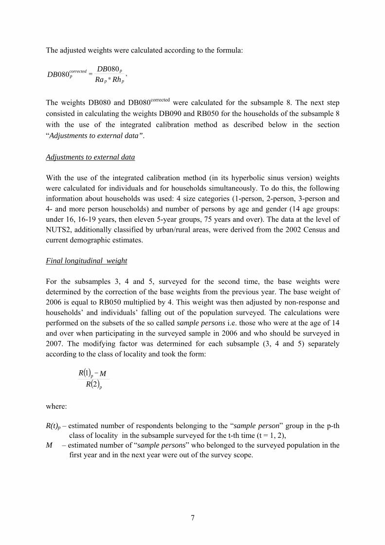
The adjusted weights were calculated according to the formula:

,080

080 RhRaDB

DBpp

pcorrectedp ∗

=

The weights DB080 and DB080corrected were calculated for the subsample 8. The next step consisted in calculating the weights DB090 and RB050 for the households of the subsample 8 with the use of the integrated calibration method as described below in the section “Adjustments to external data”. Adjustments to external data With the use of the integrated calibration method (in its hyperbolic sinus version) weights were calculated for individuals and for households simultaneously. To do this, the following information about households was used: 4 size categories (1-person, 2-person, 3-person and 4- and more person households) and number of persons by age and gender (14 age groups: under 16, 16-19 years, then eleven 5-year groups, 75 years and over). The data at the level of NUTS2, additionally classified by urban/rural areas, were derived from the 2002 Census and current demographic estimates. Final longitudinal weight For the subsamples 3, 4 and 5, surveyed for the second time, the base weights were determined by the correction of the base weights from the previous year. The base weight of 2006 is equal to RB050 multiplied by 4. This weight was then adjusted by non-response and households’ and individuals’ falling out of the population surveyed. The calculations were performed on the subsets of the so called sample persons i.e. those who were at the age of 14 and over when participating in the surveyed sample in 2006 and who should be surveyed in 2007. The modifying factor was determined for each subsample (3, 4 and 5) separately according to the class of locality and took the form:

( )

( )21R

MR

p

p −

where: R(t)p – estimated number of respondents belonging to the “sample person” group in the p-th

class of locality in the subsample surveyed for the t-th time (t = 1, 2), M – estimated number of “sample persons” who belonged to the surveyed population in the

first year and in the next year were out of the survey scope.

8

The base weights of 2006 were used for the calculation of numerator and denominator. The above expression is the reciprocal of the empirical estimate of probability that a given person will be interviewed again in the second year of the survey. In the second stage of the base weight calculation for the second year of the survey children of “sample persons” received the weights of mothers and “co-residents’ i.e. additional persons included in the household surveyed were ascribed zero weights. Then the respondents’ weights were averaged and all the members of a given household were ascribed such a mean weight. To the base weights thus obtained the trimming of extreme weights was applied. Adjustment to external data was not made. The panel weight RB062 was calculated by dividing the base weights by 3. Non-response adjustments – subsequent waves Third wave For the subsamples 4 and 5 surveyed for the third time and the subsample 6 surveyed for the second time the base weights were determined by the correction of the base weights from the previous year. For the subsample 6 the following method was applied: The base weight of 2007 is equal to RB050 multiplied by 4. This weight was then adjusted by non-response and households’ and individuals’ falling out of the population surveyed. The calculations were made on the subsamples of the so called sample persons i.e. those who were at the age of 14 and over when participating in the surveyed sample in 2007 and who should be surveyed in 2008. The modifying factor was determined according to the class of locality and took the form:

( )

( )21R

MR

p

p −

where: R(t)p – estimated number of respondents belonging to the sample person group in the p-th

class of locality in the subsample surveyed for the t-th time, M – estimated number of sample persons who belonged to the surveyed population in the first

year and in the next year were out of the survey scope. The base weights of 2007 were used for the calculation of numerator and denominator. The above expression is the reciprocal of the empirical estimate of probability that a given person will be interviewed again in the second year of the survey. In the second stage of the base weight calculation for the second year of the survey children of “sample persons” received the weights of mothers and “co-residents’ i.e. additional persons included in the household surveyed were ascribed zero weights.

9

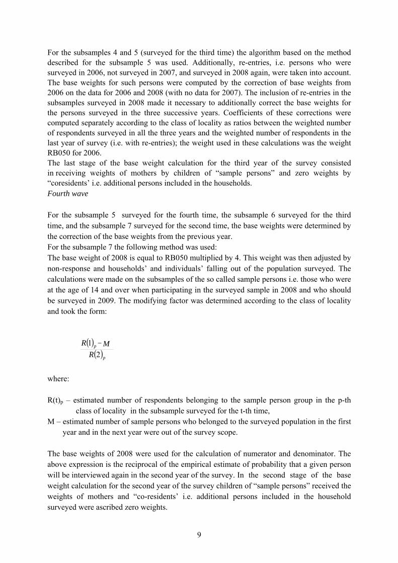
For the subsamples 4 and 5 (surveyed for the third time) the algorithm based on the method described for the subsample 5 was used. Additionally, re-entries, i.e. persons who were surveyed in 2006, not surveyed in 2007, and surveyed in 2008 again, were taken into account. The base weights for such persons were computed by the correction of base weights from 2006 on the data for 2006 and 2008 (with no data for 2007). The inclusion of re-entries in the subsamples surveyed in 2008 made it necessary to additionally correct the base weights for the persons surveyed in the three successive years. Coefficients of these corrections were computed separately according to the class of locality as ratios between the weighted number of respondents surveyed in all the three years and the weighted number of respondents in the last year of survey (i.e. with re-entries); the weight used in these calculations was the weight RB050 for 2006. The last stage of the base weight calculation for the third year of the survey consisted in receiving weights of mothers by children of “sample persons” and zero weights by “coresidents’ i.e. additional persons included in the households. Fourth wave For the subsample 5 surveyed for the fourth time, the subsample 6 surveyed for the third time, and the subsample 7 surveyed for the second time, the base weights were determined by the correction of the base weights from the previous year. For the subsample 7 the following method was used: The base weight of 2008 is equal to RB050 multiplied by 4. This weight was then adjusted by non-response and households’ and individuals’ falling out of the population surveyed. The calculations were made on the subsamples of the so called sample persons i.e. those who were at the age of 14 and over when participating in the surveyed sample in 2008 and who should be surveyed in 2009. The modifying factor was determined according to the class of locality and took the form:

( )

( )21R

MR

p

p −

where: R(t)p – estimated number of respondents belonging to the sample person group in the p-th

class of locality in the subsample surveyed for the t-th time, M – estimated number of sample persons who belonged to the surveyed population in the first

year and in the next year were out of the survey scope. The base weights of 2008 were used for the calculation of numerator and denominator. The above expression is the reciprocal of the empirical estimate of probability that a given person will be interviewed again in the second year of the survey. In the second stage of the base weight calculation for the second year of the survey children of “sample persons” received the weights of mothers and “co-residents’ i.e. additional persons included in the household surveyed were ascribed zero weights.

10

For the subsamples 5 and 6 (surveyed for the fourth and third time respectively) the algorithm based on the method described for the subsample 7 was used. Additionally, re-entries, i.e. persons who were surveyed in 2007, not surveyed in 2008, and surveyed in 2009 again, were taken into account. The base weights for such persons were computed by the correction of the base weights from 2007 on the data for 2007 and 2009 (with no data for 2008). The inclusion of re-entries in the subsamples surveyed in 2009 brought about the necessity to additionally correct the base weights for persons surveyed in the three successive years. Coefficients of these corrections were computed separately according to the class of locality as ratios betweeen the weighted number of respondents surveyed in all the three years and the weighted number of respondents in the last year of the survey (i.e. with re-entries); the weight used in these calculations was the weight RB050 for 2007. Adjustments to external data Adjustment to external data was not applied. Final longitudinal weight The panel weight RB062 was calculated: 1) by taking the base weights for subsamples 5, 6 and 7, 2) by giving a zero value to people not present in the two waves (like for example the

newly born), 3) by dividing the obtained weights by 3. The panel weight RB063 was calculated with a similar procedure, that is: 1) by taking the base weights for subsamples 5 and 6, 2) by giving a zero value to people not present in the three waves, 3) by dividing the obtained weights by 2. The panel weight RB064 was also calculated with a similar procedure, that is: 1) by taking the base weights for the subsample 5, 2) by giving a zero value to people not present in the four waves. Final household cross-sectional weight The last stage of calculations consisted in combining the four independent subsamples, applying the integrated calibration and trimming of extreme weights. As a result the following cross-sectional weights were calculated for households and individuals from the samples 2, 3, 4 and 5 in EU-SILC 2006: DB090 – weight for households, RB050 – weight for all household members but RB050ij = DB090i

11

where: i – household number, j – person number in the i-th household. PB040 – weight for respondents at the age of 16 and over who had individual interviews. This

weight is obtained by the adjustment of RB050 separately in the groups according to gender and age in each voivodship by urban and rural area,

RL070 – weight for children at the age of 0–12 years. It is obtained by the adjustment

of RB050 weight in 26 groups, i.e. 13 years of birth and gender. Final cross-sectional weights for EU-SILC 2007 were calculated in a similar way for households and individuals from the samples 3, 4, 5 and 6. This is documented in the EU-SILC 2007 Intermediate Quality Report. Final cross-sectional weights for EU-SILC 2008 were calculated in a similar way for households and individuals from the samples 4, 5, 6 and 7. This is documented in the EU-SILC 2008 Intermediate Quality Report. Final cross-sectional weights for EU-SILC 2009 were calculated in a similar way for households and individuals from the samples 5, 6, 7 and 8. This is documented in the EU-SILC 2008 Intermediate Quality Report. 2.1.9. Substitutions No substitution was applied if the household did not enter the survey.

12

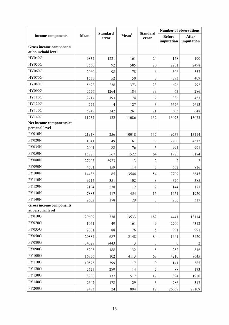
2.2. Sampling errors Standard error and effective sample size Estimation of standard errors was based on the resampling approach. We used a bootstrap method which resamples 500 times from each stratum 1−hn PSUs (primary sampling units) with replacement (McCarthy and Snowden method (1985)), where hn the number of PSUs selected for the sample size selected from each PSUs in the hth stratum. After resampling the original weights were properly rescaled and bootstrap variance estimate of the corresponding indicator was obtained by the usual Monte Carlo approximation based on the independent bootstrap replicates. Computations were carried out using SAS software. Additionally, we implemented the linearization method of variance estimation for the main poverty indicators, and the results were similar to those obtained with the bootstrap method. Cross-sectional component The mean, the total number of observations (before and after imputation) and the standard errors for the following income components

Number of observations Income components Mean1 Standard

error Mean2 Standard error Before

imputation After

imputationTotal household gross income (HY010) 50304 500 50299 500 4196 13223Total disposable household income (HY020) 38829 373 38825 372 8797 13223Total disposable household income before social transfers other than old-age and survivor’s benefits (HY022) 37061 373 36694 372 8821 13097Total disposable household income including old-age and survivor’s benefits (HY023) 31409 425 28070 389 7848 11815Net income components at household level HY040N 8507 1024 139 20 116 190HY050N 3415 84 562 19 2361 2498HY060N 2060 98 78 6 506 537HY070N 1535 52 50 3 393 409HY080N 5692 238 373 23 696 792HY090N 6153 1026 150 27 152 286HY110N 2554 171 69 6 432 453HY120N 224 4 127 3 0 7613HY130N 5248 342 261 21 603 648HY140N 11614 128 11456 128 13066 13066HY145N -820 37 -370 17 0 5800

1 Taking into account only households/persons receiving such income. 2 Taking into account whole population (households/persons) surveyed.

13



imputation After

imputationGross income components at household level HY040G 9837 1221 161 24 158 190HY050G 3550 92 585 20 2231 2498HY060G 2060 98 78 6 506 537HY070G 1535 52 50 3 393 409HY080G 5692 238 373 23 696 792HY090G 7556 1264 184 33 63 286HY110G 2717 193 74 7 386 453HY120G 224 4 127 3 6626 7613HY130G 5248 342 261 21 603 648HY140G 11237 132 11086 132 13073 13073Net income components at personal level

PY010N 21918 256 10018 137 9737 13114PY020N 1041 49 161 9 2700 4312PY035N 2001 88 76 5 991 991PY050N 15885 567 1522 64 1985 3174PY080N 27903 6923 3 2 2 2PY090N 4501 159 114 7 652 816PY100N 14436 85 3544 54 7709 8645PY110N 9214 351 102 8 326 385PY120N 2194 238 12 2 144 173PY130N 7883 117 454 15 1651 1920PY140N 2602 178 29 3 286 317Gross income components at personal level

PY010G 29609 338 13533 182 4441 13114PY020G 1041 49 161 9 2700 4312PY035G 2001 88 76 5 991 991PY050G 20884 687 2148 84 1641 3420PY080G 34028 8443 3 3 0 2PY090G 5208 188 132 8 252 816PY100G 16756 102 4113 63 4210 8645PY110G 10575 399 117 9 141 385PY120G 2527 289 14 2 88 173PY130G 8980 137 517 17 894 1920PY140G 2602 178 29 3 286 317PY200G 2483 24 894 12 26058 28109

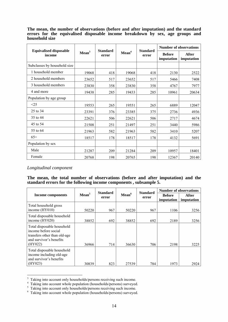
14

The mean, the number of observations (before and after imputation) and the standard errors for the equivalised disposable income breakdown by sex, age groups and household size

Number of observations Equivalised disposable

income Mean3 Standard error Mean4 Standard

error Before imputation

After imputation

Subclasses by household size

1 household member 19068 418 19068 418 2130 2522 2 household members 23652 517 23652 517 5466 7408 3 household members 23830 358 23830 358 4767 7977 4 and more 19438 285 19433 285 10961 20634Population by age group

<25 19553 265 19551 265 6889 12047 25 to 34 23391 376 23385 375 2736 4936 35 to 44 22621 506 22621 506 2717 4674 45 to 54 21508 251 21497 251 3440 5986 55 to 64 21963 582 21963 582 3410 5207 65+ 18517 178 18517 178 4132 5691Population by sex Male 21287 209 21284 209 10957 18401 Female 20768 198 20765 198 12367 20140 Longitudinal component The mean, the total number of observations (before and after imputation) and the standard errors for the following income components , subsample 5.



imputation After

imputationTotal household gross income (HY010) 50220 967 50220 967 1106 3256Total disposable household income (HY020) 38852 692 38852 692 2189 3256Total disposable household income before social transfers other than old-age and survivor’s benefits (HY022) 36966 714 36630 706 2198 3225Total disposable household income including old-age and survivor’s benefits (HY023) 30839 823 27539 784 1973 2924

3 Taking into account only households/persons receiving such income. 4 Taking into account whole population (households/persons) surveyed. 5 Taking into account only households/persons receiving such income. 6 Taking into account whole population (households/persons) surveyed.

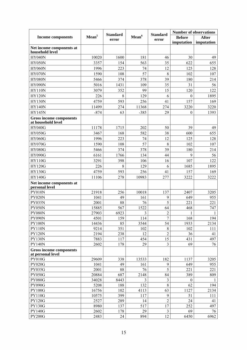
15



imputation After

imputationNet income components at household level HY040N 10020 1600 181 46 30 49HY050N 3357 154 563 35 622 655HY060N 1996 223 74 12 125 128HY070N 1590 108 57 8 102 107HY080N 5466 374 378 39 180 214HY090N 5016 1431 109 35 31 56HY110N 3079 352 99 15 120 122HY120N 226 8 129 6 0 1895HY130N 4759 593 256 41 157 169HY140N 11499 274 11368 274 3220 3220HY145N -874 63 -385 29 0 1393Gross income components at household level HY040G 11178 1715 202 50 39 49HY050G 3467 168 582 38 600 655HY060G 1996 223 74 12 125 128HY070G 1590 108 57 8 102 107HY080G 5466 374 378 39 180 214HY090G 6161 1766 134 44 9 56HY110G 3291 398 106 16 107 122HY120G 226 8 129 6 1685 1895HY130G 4759 593 256 41 157 169HY140G 11106 278 10983 277 3222 3222Net income components at personal level PY010N 21918 256 10018 137 2407 3205PY020N 1041 49 161 9 649 955PY035N 2001 88 76 5 221 221PY050N 15885 567 1522 64 468 747PY080N 27903 6923 3 2 1 1PY090N 4501 159 114 7 168 194PY100N 14436 85 3544 54 1933 2134PY110N 9214 351 102 8 102 111PY120N 2194 238 12 2 36 41PY130N 7883 117 454 15 431 497PY140N 2602 178 29 3 69 76Gross income components at personal level PY010G 29609 338 13533 182 1137 3205PY020G 1041 49 161 9 649 955PY035G 2001 88 76 5 221 221PY050G 20884 687 2148 84 389 809PY080G 34028 8443 3 3 0 1PY090G 5208 188 132 8 62 194PY100G 16756 102 4113 63 1127 2134PY110G 10575 399 117 9 51 111PY120G 2527 289 14 2 24 41PY130G 8980 137 517 17 252 497PY140G 2602 178 29 3 69 76PY200G 2483 24 894 12 6450 6962

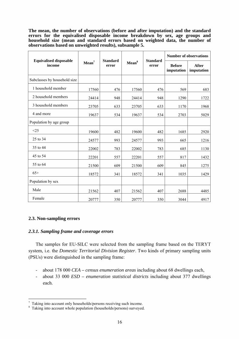
16

The mean, the number of observations (before and after imputation) and the standard errors for the equivalised disposable income breakdown by sex, age groups and household size (mean and standard errors based on weighted data, the number of observations based on unweighted results), subsample 5.

Number of observations Equivalised disposable

income Mean7 Standard error Mean8 Standard

error Before imputation

After imputation

Subclasses by household size

1 household member 17560 476 17560 476 569 683

2 household members 24414 948 24414 948 1290 1722

3 household members 23705 633 23705 633 1170 1968

4 and more 19637 534 19637 534 2703 5029

Population by age group

<25 19600 482 19600 482 1685 2920

25 to 34 24577 993 24577 993 665 1216

35 to 44 22002 783 22002 783 685 1130

45 to 54 22201 557 22201 557 817 1432

55 to 64 21500 609 21500 609 845 1275

65+ 18572 341 18572 341 1035 1429

Population by sex

Male 21562 407 21562 407 2688 4485

Female 20777 350 20777 350 3044 4917 2.3. Non-sampling errors 2.3.1. Sampling frame and coverage errors

The samples for EU-SILC were selected from the sampling frame based on the TERYT system, i.e. the Domestic Territorial Division Register. Two kinds of primary sampling units (PSUs) were distinguished in the sampling frame:

- about 178 000 CEA – census enumeration areas including about 68 dwellings each, - about 33 000 ESD – enumeration statistical districts including about 377 dwellings

each.

7 Taking into account only households/persons receiving such income. 8 Taking into account whole population (households/persons) surveyed.

17

The whole territory of Poland is divided into enumeration statistical districts and census enumeration areas. In EU-SILC census enumeration areas are used as primary sampling units. The secondary sampling units are dwellings. For each census enumeration area a list of dwellings was made up to form the secondary sampling frame. All the households from the selected dwellings are supposed to enter the survey. The TERYT system is updated annually with respect to the territorial division into statistical districts and census enumeration areas. The lists of dwellings, names of towns, villages and streets are updated. Other changes due to new construction, dismantle of buildings and administrative division modifications are also introduced. In the longitudinal (panel) component consisting of the subsample 5, some 6.2% of dwellings were found to be non-existing (cancelled, changed for non-residential units), uninhabited or temporarily inhabited. 2.3.2. Measurement and processing errors Very much like any other statistical survey, EU-SILC may be burdened with non-sampling errors which occur at various stages of the survey and which cannot be eliminated completely. This mainly applies to interviewers’ errors at the stage of collecting the information, errors due to the respondents’ misunderstanding of questions and inaccurate or sometimes even false answers as well as the errors taking place at the stage of data recording. For EU-SILC 2006 it is possible to state that about three quarters of respondents (78% of those filling in the household questionnaire and 75% of those filling in the individual questionnaire) showed a favourable attitude towards the survey, while about 3% (both in the case of the household and individual interview) were unwilling towards it. In the interviewers’ opinion, in about 88% of questionnaires (both household and individual ones) the quality of non-income data collected could be recognised as good or very good and in 1% - as doubtful. For EU-SILC 2007 and EU-SILC 2008 the figures were almost the same, about three quarters of respondents (80% of those filling in the household questionnaire and 78% of those filling in the individual questionnaire) showed a favourable attitude towards the survey, while about 3% (both in the case of the household and individual interview) were unwilling towards it. In the interviewers’ opinion, in about 89% of questionnaires (both household and individual ones) the quality of non-income data collected could be recognised as good or very good and in 1% - as doubtful. For EU-SILC 2009 about three quarters of respondents (83% of those filling in the household questionnaire and 81% of those filling in the individual questionnaire) showed a favourable attitude towards the survey, while about 2% (both in the case of the household and individual interview) were unwilling towards it. In the interviewers’ opinion, in about 74% of questionnaires (both household and individual ones) the quality of non-income data collected could be recognised as good or very good and in 2% - as doubtful. The quality of income data in 2006, 2007, 2008 and 2009 was evaluated as slightly worse, mainly because of item non-response. It should also be pointed out that, in our opinion, the quality of data concerning net income categories is much higher than that of gross income. This is due to the fact that non-response was much more frequent for the information on taxes and social and health insurance contributions.

18

In Poland EU-SILC was carried out in May/June 2006, 2007, 2008 and 2009. During the years 2006, 2007, 2008 and 2009 the data collection was performed by a face-to-face interview technique with the use of paper form questionnaires (the so called PAPI method). Two types of questionnaire: individual and household questionnaire were applicable. The organisation and performance of the survey in the field was within the responsibility of regional statistical offices. Many interviewers were regular employees of the statistical offices and had experience in other social surveys. Survey performance in the field was preceded by a series of trainings organised in 2006, 2007, 2008 and 2009. Regional survey coordinators were instructed by CSO Social Statistics Division staff members and then the regional survey coordinators trained the interviewers at the regional statistical offices. Interviewers’ visits to households were preceded by the introductory letter of the CSO President. The interviewers received written instructions concerning the survey performance. Small gifts were given to the families participating in the survey. Each statistical office chose the type of gift for its respondents. Data recording and check-up took place in regional statistical offices and was done with the use of Microsoft Visual FoxPro. After all the questionnaires for a given household had been recorded (the identifiers being voivodship number, dwelling number and household number), it was possible to make the household screening which consisted of logical and calculation check-up at the section, inter-section and inter-questionnaire levels. The regional files were then transferred to the CSO Computing Centre and combined to make up the general files at the national level. The national file completeness was also checked with the use of Microsoft Visual FoxPro. Additional check-up was made with SAS checking programmes. On the basis of overall data files it was possible to create files for Eurostat. Some of the primary target variables could be found directly in the questionnaires, others had to be calculated with the algorithms especially prepared for this purpose. The tables of EU-SILC results were compiled with the use of: SAS, SPSS, Microsoft Visual FoxPro. 2.3.3. Non-response errors Achieved sample size subsample 5:

Sample size wave

1 2 3 4

A 4105 3632 3452 3256

B 9452 8396 7936 7401 A - number of households for which an interview is accepted for the database B - number of persons of 16 years or older who are members of the households for which the

interview is accepted for the database, and who completed a personal interview

19

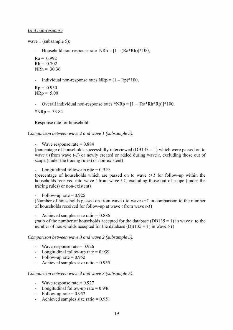
Unit non-response wave 1 (subsample 5):

- Household non-response rate NRh = [1 – (Ra*Rh)]*100,

Ra = 0.992 Rh = 0.702 NRh = 30.36 - Individual non-response rates NRp = (1 – Rp)*100,

Rp = 0.950 NRp = 5.00 - Overall individual non-response rates *NRp = [1 – (Ra*Rh*Rp)]*100,

*NRp = 33.84 Response rate for household:

Comparison between wave 2 and wave 1 (subsample 5).

- Wave response rate = 0.884 (percentage of households successfully interviewed (DB135 = 1) which were passed on to wave t (from wave t-1) or newly created or added during wave t, excluding those out of scope (under the tracing rules) or non-existent) - Longitudinal follow-up rate = 0.919 (percentage of households which are passed on to wave t+1 for follow-up within the households received into wave t from wave t-1, excluding those out of scope (under the tracing rules) or non-existent) - Follow-up rate = 0.925 (Number of households passed on from wave t to wave t+1 in comparison to the number of households received for follow-up at wave t from wave t-1) - Achieved samples size ratio = 0.886 (ratio of the number of households accepted for the database (DB135 = 1) in wave t to the number of households accepted for the database (DB135 = 1) in wave t-1)


- Wave response rate = 0.926 - Longitudinal follow-up rate = 0.939 - Follow-up rate = 0.952 - Achieved samples size ratio = 0.955


- Wave response rate = 0.927 - Longitudinal follow-up rate = 0.946 - Follow-up rate = 0.952 - Achieved samples size ratio = 0.951

20

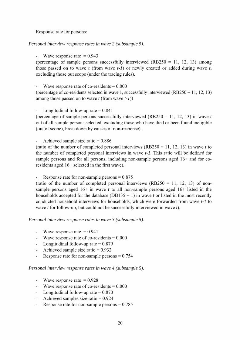
Response rate for persons:

Personal interview response rates in wave 2 (subsample 5). - Wave response rate = 0.943 (percentage of sample persons successfully interviewed (RB250 = 11, 12, 13) among those passed on to wave t (from wave t-1) or newly created or added during wave t, excluding those out scope (under the tracing rules).

- Wave response rate of co-residents = 0.000 (percentage of co-residents selected in wave 1, successfully interviewed (RB250 = 11, 12, 13) among those passed on to wave t (from wave t-1)) - Longitudinal follow-up rate = 0.841 (percentage of sample persons successfully interviewed (RB250 = 11, 12, 13) in wave t out of all sample persons selected, excluding those who have died or been found ineligible (out of scope), breakdown by causes of non-response). - Achieved sample size ratio = 0.886 (ratio of the number of completed personal interviews (RB250 = 11, 12, 13) in wave t to the number of completed personal interviews in wave t-1. This ratio will be defined for sample persons and for all persons, including non-sample persons aged 16+ and for co-residents aged 16+ selected in the first wave). - Response rate for non-sample persons = 0.875 (ratio of the number of completed personal interviews (RB250 = 11, 12, 13) of non-sample persons aged 16+ in wave t to all non-sample persons aged 16+ listed in the households accepted for the database (DB135 = 1) in wave t or listed in the most recently conducted household interviews for households, which were forwarded from wave t-1 to wave t for follow-up, but could not be successfully interviewed in wave t).

Personal interview response rates in wave 3 (subsample 5).

- Wave response rate = 0.941 - Wave response rate of co-residents = 0.000 - Longitudinal follow-up rate = 0.879 - Achieved sample size ratio = 0.932 - Response rate for non-sample persons = 0.754

Personal interview response rates in wave 4 (subsample 5).

- Wave response rate = 0.928 - Wave response rate of co-residents = 0.000 - Longitudinal follow-up rate = 0.870 - Achieved samples size ratio = 0.924 - Response rate for non-sample persons = 0.785

21

Distribution of households by household status (DB110), by record of contact at address (DB120), by household questionnaire result (DB130) and by household interview acceptance (DB135) Wave 1 (subsample 5). Household questionnaire result

DB130 Total %

Total 5409 100.0

11 – household questionnaire completed 4105 75.9

21 – refusal to co-operate 1107 20.5

22 – entire household temporarily away for duration of fieldwork 81 1.5

23 – household unable to respond (illness, incapacity,…) 94 1.7

24 – other reasons 22 0.4

Missing 0 0.0 Household interview acceptance

DB135 Total %

Total 4105 100.0

1 – interview accepted for database 4101 99.9

2 – interview rejected 4 0.1 Wave 2 (subsample 5). Household status

DB110 Total %

Total 4135 100.0

1 – at the same address as last interview 3934 95.1

2 – entire household moved to a private household within the country 67 1.6

3 – entire household moved to a collective household or institution within the country 2 0.0

4 – household moved outside the country 8 0.2

5 – entire household died 24 0.6

6 – household does not contain sample persons 0 0.0

7 – address non-contacted (unable to access, lost - no information on record on what happened to the household) 63 1.5

8 – split –off household 34 0.8

10 – fusion 3 0.1

22

Record of contact at address

DB120 Total %

Total 101 100.0

11 – address contacted 72 71.3

21 – address cannot be located 3 3.0

22 – address unable to access 0 0.0

23 – address does not exist or is non-residential or unoccupied or is not principal residence 26 25.7

Household questionnaire result

DB130 Total %

Total 4006 100.0

11 – household questionnaire completed 3632 90.7

21 – refusal to co-operate 234 5.8

22 – entire household temporarily away for duration of fieldwork 86 2.1

23 – household unable to respond (illness, incapacity,…) 33 0.8

24 – other reasons 21 0.5

Missing 0 0.0

Household interview acceptance

DB135 Total %

Total 3632 100.0

1 – interview accepted for database 3632 100.0

2 – interview rejected 0 0.0

23

Wave 3 (subsample 5). Household status

DB110 Total %

Total 3818 100.0 1 – at the same address as last interview 3620 94.8 2 – entire household moved to a private household within the

country 78 2.0 3 – entire household moved to a collective household or

institution within the country 2 0.1 4 – household moved outside the country 6 0.2 5 – entire household died 31 0.8 6 – household does not contain sample persons 4 0.1 7 – address non-contacted (unable to access, lost - no

information on record on what happened to the household) 1 0.0 8 – split –off household 46 1.2

10 – fusion 1 0.0 11 – lost household 29 0.8 Record of contact at address

DB120 Total %

Total 124 100.0 11 – address contacted 90 72.6 21 – address cannot be located 1 0.8 22 – address unable to access 1 0.8 23 – address does not exist or is non-residential or unoccupied

or is not principal residence 32 25.8 Missing 0 0.0 Household questionnaire result

DB130 Total %

Total 3710 100.0 11 – household questionnaire completed 3452 93.0 21 – refusal to co-operate 139 3.7 22 – entire household temporarily away for duration of fieldwork 77 2.1 23 – household unable to respond (illness, incapacity,…) 28 0.8 24 – other reasons 14 0.4 Missing 0 0.0 Household interview acceptance

DB135 Total %

Total 3452 100.0 1 – interview accepted for database 3452 100.0 2 – interview rejected 0 0.0

24

Wave 4 (subsample 5). Household status

DB110 Total %

Total 3556 100.0 1 – at the same address as last interview 3422 96.2 2 – entire household moved to a private household within the

country 41 1.2 3 – entire household moved to a collective household or

institution within the country 4 0.1 4 – household moved outside the country 14 0.4 5 – entire household died 14 0.4 6 – household does not contain sample persons 2 0.1 7 – Household unable to access (due to for example climatic

conditions) 0 0.0 8 – split –off household 24 0.7

10 – fusion 1 0.0 11 – lost household (no information on record on what happened

to the household) 34 1.0 Record of contact at address

DB120 Total %

Total 65 100.0 11 – address contacted 54 83.1 21 – address cannot be located 0 0.0 22 – address unable to access 1 1.5 23 – address does not exist or is non-residential or unoccupied

or is not principal residence 10 15.4 Household questionnaire result

DB130 Total %

Total 3476 100.0 11 – household questionnaire completed 3256 93.7 21 – refusal to co-operate 127 3.7 22 – entire household temporarily away for duration of fieldwork 63 1.8 23 – household unable to respond (illness, incapacity,…) 23 0.7 24 – other reasons 7 0.2 Missing 0 0.0 Household interview acceptance

DB135 Total %

Total 3256 100.0 1 – interview accepted for database 3256 100.0 2 – interview rejected 0 0.0

25

Distribution of persons for membership status (RB110) Wave 2 (subsample 5).

Distribution of persons for membership status (RB110)

Current household members No current household members Total

RB110=1 RB110=2 RB110=3 RB110=4 RB120 = 2 to 4 RB110=6 RB110=7

Total 11289 10707 40 116 115 130 68 0

% 100.0 94.8 0.4 1.0 1.0 1.2 0.6 0.0

Distribution of persons moving out by variable RB120.

RB110 = 5 RB120 = 1 Total

A B RB120 = 2 RB120 = 3 RB120 = 4

Total 243 40 73 36 73 21

% 100.0 16.5 30.0 14.8 30.0 8.7

A – this person is a current household member in this wave

B - this person is not a current household member Wave 3 (subsample 5). Distribution of persons for membership status (RB110)



Total 10712 10019 99 138 102 122 86 0

% 100.0 93.5 0.9 1.3 1.0 1.1 0.8 0.0


RB110 = 5 RB120 = 1 Total

A B RB120 = 2 RB120 = 3 RB120 = 4

Total 268 99 47 30 73 19

% 100.0 36.9 17.5 11.2 27.3 7.1


B - this person is not a current household member

26

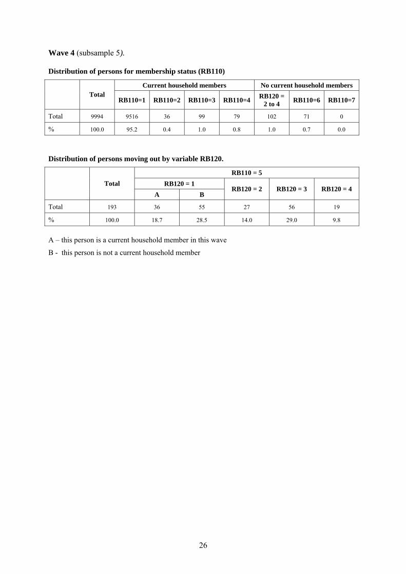
Wave 4 (subsample 5). Distribution of persons for membership status (RB110)



Total 9994 9516 36 99 79 102 71 0

% 100.0 95.2 0.4 1.0 0.8 1.0 0.7 0.0


RB110 = 5 RB120 = 1 Total

A B RB120 = 2 RB120 = 3 RB120 = 4

Total 193 36 55 27 56 19

% 100.0 18.7 28.5 14.0 29.0 9.8


B - this person is not a current household member

27

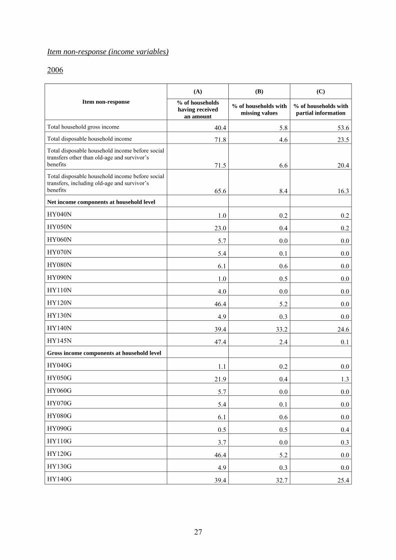
Item non-response (income variables) 2006

(A) (B) (C)

Item non-response % of households having received

an amount

% of households with missing values

% of households with partial information

Total household gross income 40.4 5.8 53.6Total disposable household income 71.8 4.6 23.5Total disposable household income before social transfers other than old-age and survivor’s benefits 71.5 6.6 20.4Total disposable household income before social transfers, including old-age and survivor’s benefits 65.6 8.4 16.3Net income components at household level

HY040N 1.0 0.2 0.2

HY050N 23.0 0.4 0.2

HY060N 5.7 0.0 0.0

HY070N 5.4 0.1 0.0

HY080N 6.1 0.6 0.0

HY090N 1.0 0.5 0.0

HY110N 4.0 0.0 0.0

HY120N 46.4 5.2 0.0

HY130N 4.9 0.3 0.0

HY140N 39.4 33.2 24.6

HY145N 47.4 2.4 0.1Gross income components at household level

HY040G 1.1 0.2 0.0

HY050G 21.9 0.4 1.3

HY060G 5.7 0.0 0.0

HY070G 5.4 0.1 0.0

HY080G 6.1 0.6 0.0

HY090G 0.5 0.5 0.4

HY110G 3.7 0.0 0.3

HY120G 46.4 5.2 0.0

HY130G 4.9 0.3 0.0

HY140G 39.4 32.7 25.4

28

% of persons 16+ having received

an amount

% of persons 16+ with missing values

% of persons 16+ with partial information

Net income components at personal level

PY010N 31.2 7.7 0.0

PY021N 0.1 0.2 0.0

PY035N 2.8 0.7 0.0

PY050N 5.9 2.8 0.4

PY080N 0.0 0.0 0.0

PY090N 3.2 0.3 0.0

PY100N 21.6 1.9 0.3

PY110N 1.4 0.1 0.0

PY120N 0.4 0.0 0.0

PY130N 6.1 0.7 0.1

PY140N 1.4 0.1 0.0

Gross income components at personal level

PY010G 16.0 7.7 15.3

PY021G 0.1 0.2 0.0

PY035G 2.8 0.7 0.0

PY050G 5.1 2.0 3.2

PY080G 0.0 0.0 0.0

PY090G 2.0 0.3 1.2

PY100G 15.1 1.9 6.8

PY110G 0.9 0.1 0.5

PY120G 0.2 0.0 0.2

PY130G 4.3 0.7 1.9

PY140G 1.4 0.1 0.0

29

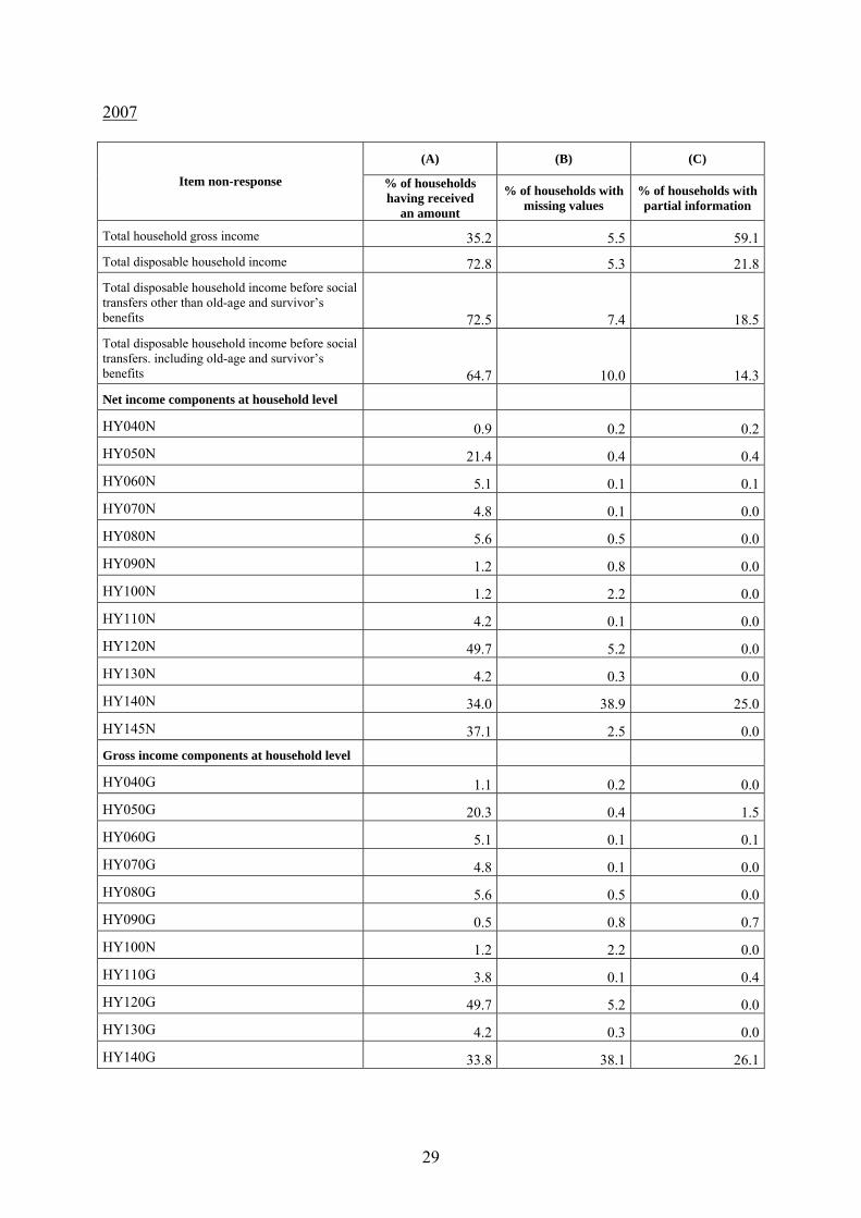
2007

(A) (B) (C)


an amount



Total household gross income 35.2 5.5 59.1Total disposable household income 72.8 5.3 21.8Total disposable household income before social transfers other than old-age and survivor’s benefits 72.5 7.4 18.5Total disposable household income before social transfers. including old-age and survivor’s benefits 64.7 10.0 14.3Net income components at household level

HY040N 0.9 0.2 0.2

HY050N 21.4 0.4 0.4

HY060N 5.1 0.1 0.1

HY070N 4.8 0.1 0.0

HY080N 5.6 0.5 0.0

HY090N 1.2 0.8 0.0

HY100N 1.2 2.2 0.0

HY110N 4.2 0.1 0.0

HY120N 49.7 5.2 0.0

HY130N 4.2 0.3 0.0

HY140N 34.0 38.9 25.0

HY145N 37.1 2.5 0.0Gross income components at household level

HY040G 1.1 0.2 0.0

HY050G 20.3 0.4 1.5

HY060G 5.1 0.1 0.1

HY070G 4.8 0.1 0.0

HY080G 5.6 0.5 0.0

HY090G 0.5 0.8 0.7

HY100N 1.2 2.2 0.0

HY110G 3.8 0.1 0.4

HY120G 49.7 5.2 0.0

HY130G 4.2 0.3 0.0

HY140G 33.8 38.1 26.1

30


an amount




PY010N 31.7 7.9 0.1

PY020N 7.7 2.9 1.0

PY021N 0.2 0.2 0.0

PY035N 2.6 0.7 0.0

PY050N 5.8 2.9 0.3

PY070N 6.1 1.3 0.0

PY080N 0.0 0.0 0.0

PY090N 2.5 0.4 0.0

PY100N 22.8 1.9 0.2

PY110N 1.2 0.2 0.0

PY120N 0.4 0.0 0.0

PY130N 5.8 0.6 0.0

PY140N 1.4 0.1 0.0


PY010G 15.5 7.9 16.3

PY020N 7.7 2.9 1.0

PY021G 0.2 0.2 0.0

PY030G 0.0 19.8 2.7

PY035G 2.6 0.7 0.0

PY050G 5.8 2.3 2.8

PY070N 6.1 1.3 0.0

PY080G 0.0 0.0 0.0

PY090G 1.2 0.4 1.3

PY100G 13.2 1.9 9.8

PY110G 0.6 0.2 0.7

PY120G 0.2 0.0 0.2

PY130G 2.9 0.6 2.9

PY140G 1.4 0.1 0.0

31

2008

(A) (B) (C)


an amount



Total household gross income 33.7 7.0 59.1

Total disposable household income 69.3 6.7 23.9

Total disposable household income before social transfers other than old-age and survivor’s benefits 69.4 8.8 20.5

Total disposable household income before social transfers, including old-age and survivor’s benefits 62.0 12.2 15.1

Net income components at household level

HY040N 0.9 0.2 0.3

HY050N 19.4 0.5 0.5

HY060N 4.3 0.2 0.0

HY070N 3.7 0.1 0.0

HY080N 5.0 0.7 0.0

HY081N 2.2 0.2 0.0

HY090N 1.2 0.8 0.0

HY100N 1.2 2.6 0.0

HY110N 3.7 0.1 0.0

HY120N 50.7 5.6 0.0

HY130N 4.4 0.3 0.0

HY131N 1.1 0.1 0.0

HY140N 33.2 41.7 23.4

HY145N 33.8 3.5 0.1

Gross income components at household level

HY040G 1.1 0.2 0.0

HY050G 18.4 0.5 1.4

HY060G 4.3 0.2 0.0

HY070G 3.7 0.1 0.0

HY080G 5.0 0.7 0.0

HY081G 2.2 0.2 0.0

HY090G 0.5 0.8 0.7

HY100G 1.2 2.6 0.0

HY110G 3.4 0.1 0.4

HY120G 50.7 5.6 0.0

HY130G 4.4 0.3 0.0

HY131G 1.1 0.1 0.0

HY140G 33.0 41.1 24.3

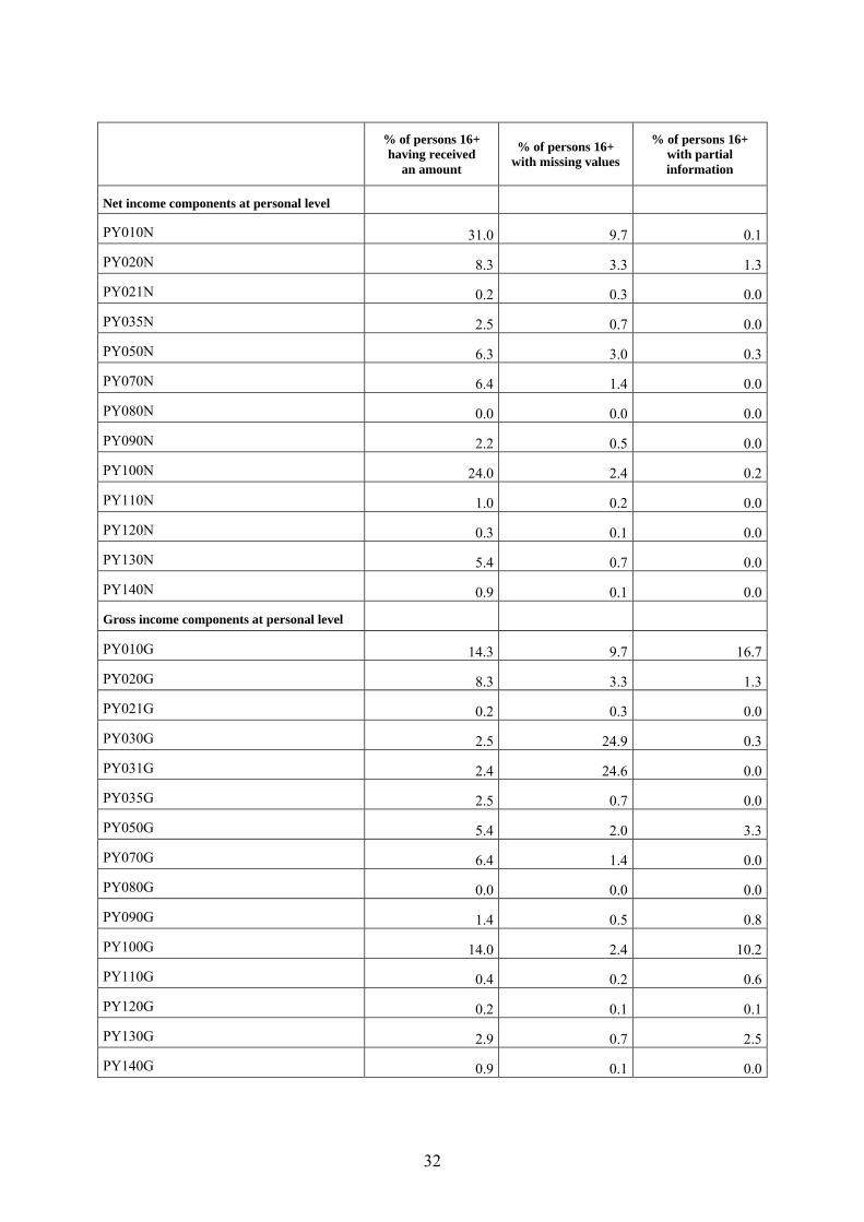
32


an amount




PY010N 31.0 9.7 0.1

PY020N 8.3 3.3 1.3

PY021N 0.2 0.3 0.0

PY035N 2.5 0.7 0.0

PY050N 6.3 3.0 0.3

PY070N 6.4 1.4 0.0

PY080N 0.0 0.0 0.0

PY090N 2.2 0.5 0.0

PY100N 24.0 2.4 0.2

PY110N 1.0 0.2 0.0

PY120N 0.3 0.1 0.0

PY130N 5.4 0.7 0.0

PY140N 0.9 0.1 0.0


PY010G 14.3 9.7 16.7

PY020G 8.3 3.3 1.3

PY021G 0.2 0.3 0.0

PY030G 2.5 24.9 0.3

PY031G 2.4 24.6 0.0

PY035G 2.5 0.7 0.0

PY050G 5.4 2.0 3.3

PY070G 6.4 1.4 0.0

PY080G 0.0 0.0 0.0

PY090G 1.4 0.5 0.8

PY100G 14.0 2.4 10.2

PY110G 0.4 0.2 0.6

PY120G 0.2 0.1 0.1

PY130G 2.9 0.7 2.5

PY140G 0.9 0.1 0.0

33

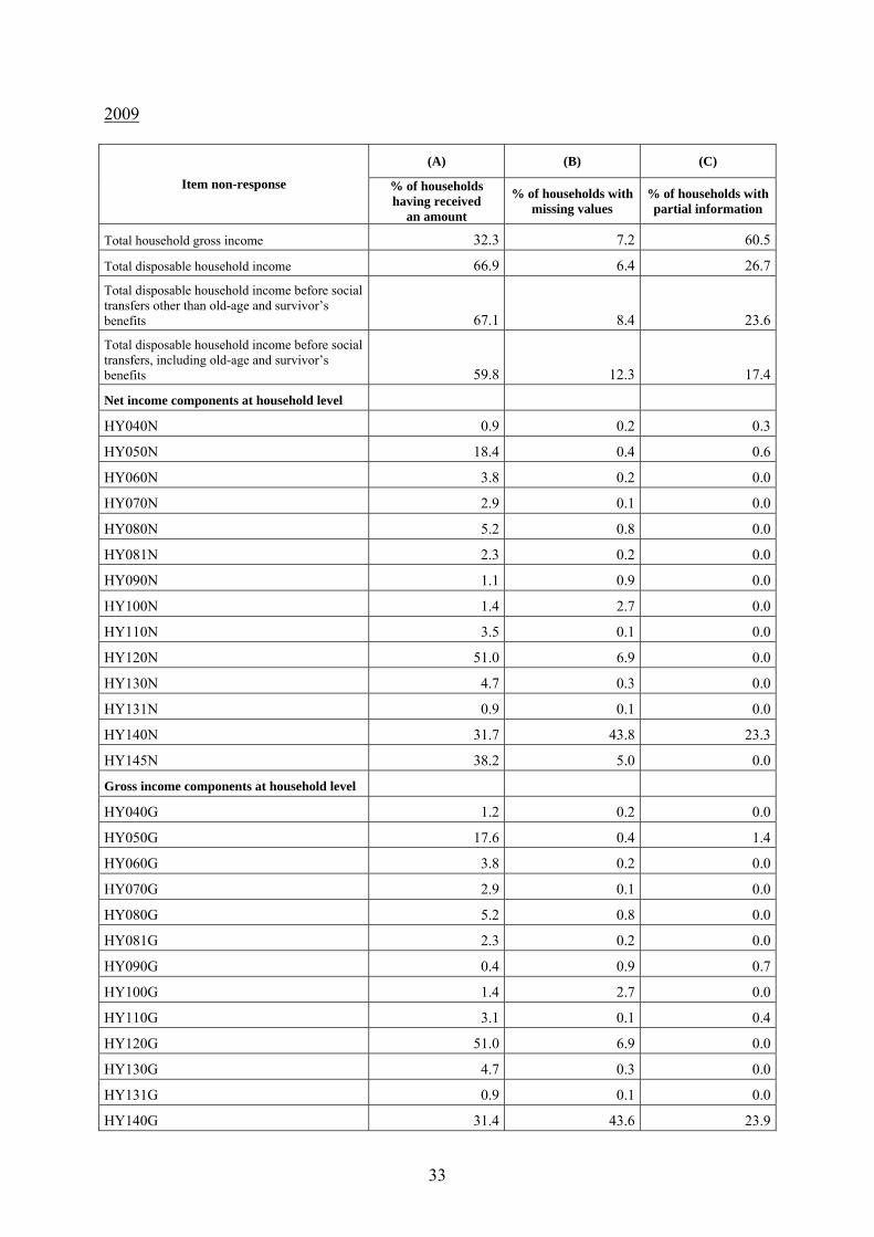
2009

(A) (B) (C)


an amount



Total household gross income 32.3 7.2 60.5

Total disposable household income 66.9 6.4 26.7

Total disposable household income before social transfers other than old-age and survivor’s benefits 67.1 8.4 23.6

Total disposable household income before social transfers, including old-age and survivor’s benefits 59.8 12.3 17.4

Net income components at household level

HY040N 0.9 0.2 0.3

HY050N 18.4 0.4 0.6

HY060N 3.8 0.2 0.0

HY070N 2.9 0.1 0.0

HY080N 5.2 0.8 0.0

HY081N 2.3 0.2 0.0

HY090N 1.1 0.9 0.0

HY100N 1.4 2.7 0.0

HY110N 3.5 0.1 0.0

HY120N 51.0 6.9 0.0

HY130N 4.7 0.3 0.0

HY131N 0.9 0.1 0.0

HY140N 31.7 43.8 23.3

HY145N 38.2 5.0 0.0

Gross income components at household level

HY040G 1.2 0.2 0.0

HY050G 17.6 0.4 1.4

HY060G 3.8 0.2 0.0

HY070G 2.9 0.1 0.0

HY080G 5.2 0.8 0.0

HY081G 2.3 0.2 0.0

HY090G 0.4 0.9 0.7

HY100G 1.4 2.7 0.0

HY110G 3.1 0.1 0.4

HY120G 51.0 6.9 0.0

HY130G 4.7 0.3 0.0

HY131G 0.9 0.1 0.0

HY140G 31.4 43.6 23.9

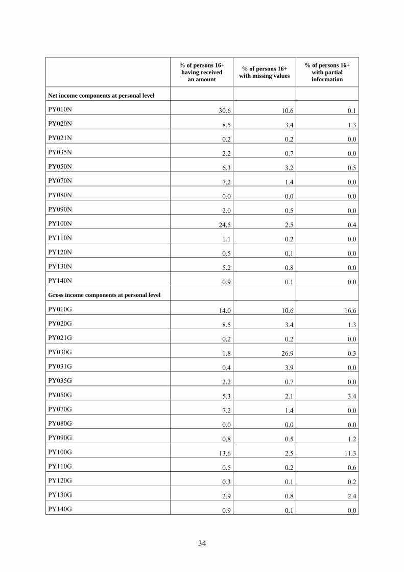
34


an amount




PY010N 30.6 10.6 0.1

PY020N 8.5 3.4 1.3

PY021N 0.2 0.2 0.0

PY035N 2.2 0.7 0.0

PY050N 6.3 3.2 0.5

PY070N 7.2 1.4 0.0

PY080N 0.0 0.0 0.0

PY090N 2.0 0.5 0.0

PY100N 24.5 2.5 0.4

PY110N 1.1 0.2 0.0

PY120N 0.5 0.1 0.0

PY130N 5.2 0.8 0.0

PY140N 0.9 0.1 0.0


PY010G 14.0 10.6 16.6

PY020G 8.5 3.4 1.3

PY021G 0.2 0.2 0.0

PY030G 1.8 26.9 0.3

PY031G 0.4 3.9 0.0

PY035G 2.2 0.7 0.0

PY050G 5.3 2.1 3.4

PY070G 7.2 1.4 0.0

PY080G 0.0 0.0 0.0

PY090G 0.8 0.5 1.2

PY100G 13.6 2.5 11.3

PY110G 0.5 0.2 0.6

PY120G 0.3 0.1 0.2

PY130G 2.9 0.8 2.4

PY140G 0.9 0.1 0.0

35

2.4. Mode of data collection EU-SILC is a non-obligatory, representative survey of individual households, performed by a face-to-face interview technique with the use of paper form questionnaires (the so called PAPI method). Two types of questionnaire: individual and household questionnaire were applicable. Wave 1 (subsample 5). Distribution of household members by RB250 Household members 16+ (RB245 = 1 to 3)

Total RB250=11 RB250=14

Total 9951 9452 499

% 100.0 95.0 5.0

Distribution of household members by RB260 Household members 16+ (RB245 = 1 to 3 and RB250 = 11 or 13)

Total RB260 = 1 RB260 = 2 RB260 = 3 RB260 = 4 RB260 = 5

Total 9452 7771 0 0 0 1681

% 100.0 82.2 0.0 0.0 0.0 17.8

Wave 2 (subsample 5). Distribution of household members by RB250 Household members 16+ (RB245 = 1 to 3)

Total RB250=11 RB250=14

Total 8909 8396 513

% 100.0 94.2 5.8

Sample persons 16+ (RB245 = 1 to 3 and RB100 = 1)

Total RB250=11 RB250=14

Total 8805 8305 500

% 100.0 94.3 5.7

Co-residents 16+ (RB245 = 1 to 3 and RB100 = 2)

Total RB250=11 RB250=14

Total 104 91 13

% 100.0 87.5 12.5

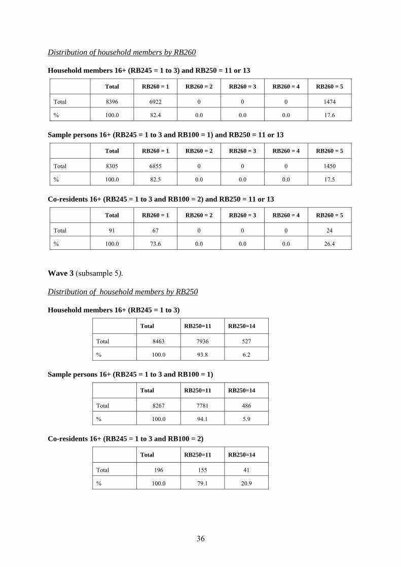
36

Distribution of household members by RB260 Household members 16+ (RB245 = 1 to 3) and RB250 = 11 or 13


Total 8396 6922 0 0 0 1474

% 100.0 82.4 0.0 0.0 0.0 17.6

Sample persons 16+ (RB245 = 1 to 3 and RB100 = 1) and RB250 = 11 or 13


Total 8305 6855 0 0 0 1450

% 100.0 82.5 0.0 0.0 0.0 17.5

Co-residents 16+ (RB245 = 1 to 3 and RB100 = 2) and RB250 = 11 or 13


Total 91 67 0 0 0 24

% 100.0 73.6 0.0 0.0 0.0 26.4


Total RB250=11 RB250=14

Total 8463 7936 527

% 100.0 93.8 6.2


Total RB250=11 RB250=14

Total 8267 7781 486

% 100.0 94.1 5.9


Total RB250=11 RB250=14

Total 196 155 41

% 100.0 79.1 20.9

37



Total 7936 6463 0 0 0 1473

% 100.0 81.4 0.0 0.0 0.0 18.6



Total 7781 6349 0 0 0 1432

% 100.0 81.6 0.0 0.0 0.0 18.4



Total 155 114 0 0 0 41

% 100.0 73.5 0.0 0.0 0.0 26.5


Total RB250=11 RB250=14

Total 8005 7401 604

% 100.0 92.5 7.5


Total RB250=11 RB250=14

Total 7626 7078 548

% 100.0 92.8 7.2


Total RB250=11 RB250=14

Total 379 323 56

% 100.0 85.2 14.8

38



Total 7401 5912 0 0 0 1489

% 100.0 79.9 0.0 0.0 0.0 20.1



Total 7078 5703 0 0 0 1375

% 100.0 80.6 0.0 0.0 0.0 19.4



Total 323 209 0 0 0 114

% 100.0 64.7 0.0 0.0 0.0 35.3

As for individual interviews, in 2006, 2007, 2008 and in 2009 a relatively high share (17.8%, 17.6%, 18.6% and 20.1%) of proxy interviews was noted. This was thoroughly discussed with the survey coordinators in the field. The interviewers decided on proxy interviews only if the substitute respondents were well informed about the situation in the household and there was no other possibility to get the information. Proxy interviews were performed in the following situations: - no contact with the respondent because of long-term absence (e.g. work in another town

or abroad); - respondent’s disability, illness or pathology (such as alcoholism); - according to other members of the household, the respondent was only available late at night

and was not willing to participate in such a long interview, while at the same time the proxy could provide detailed information, sometimes even based on the documents, such as tax statements.

2.5. Imputation procedures Imputation is aimed at obtaining complete records at the level of target variables. Target variables do not simply reflect questionnaire variables and their calculation algorithm is often complicated, although it principally consists in aggregation. So it is necessary to decide what aggregation level the imputation should take place at. There are three possible options:

- the level of questionnaire variables, - the level of partly aggregated components, - the level of ready-calculated target variables.

39

Since the only formal requirement is to obtain imputed target variables, all the above options are permissible and practicable, depending on the specific character of variables. However, the most frequent practice is the imputation at the level of questionnaire variables. There are certain arguments for this approach, on condition that the quantity of data and calculation algorithm details allow for it without much complication. First of all, imputation at the lowest aggregation level can be desirable for the principal reasons related to the quality of imputation when:

- a target variable implies components of different nature (i.e. components take different but rather predictable values, e.g. various social benefits, or they depend on different variables and thus they are easier to be modelled separately);

- target variables include many components and it is often the case that some of them have the missingvalues, while others - the correct values which would be missed during the imputation of an aggregated variable.

Secondly, there are practical arguments for the imputation of disaggregated variables, as the same data serve as a basis for the calculation of national variables differing from the Eurostat’s target variables. Thus the imputation of disaggregated components may be required so as to ensure the imputed data needed for other calculations. The imputation at the target variable level is carried out only when the above circumstances do not occur or when overcoming the practical difficulties is easier than the imputation of disaggregated data. There are several methods of component imputation. They can be classified as deterministic and stochastic methods. In the case of deterministic methods the selected method and the set of explanatory variables (algorithm) clearly determine the imputation values for each record. In stochastic methods the imputation value is determined with the use of a random component. That is why it may happen that with the same algorithm and the same data file each algorithm realisation will give slightly different imputation values. Although the stochastic methods slightly increase estimator variance (introducing an additional random error component), they do not distort variance or original data distribution characteristics and allow for the correct estimation of random error. Deterministic imputation brings about variable variance reduction in the file and random error underestimation; it also distorts to a greater extent the correlation structure (increasing correlations with explanatory variables). According to item 2.7 of Regulation 1981/2003 it is recommended that for EU-SILC imputation the methods retaining distribution characteristics should be applied, which means the preference for the stochastic methods. Out of the stochastic methods the following were used in the task presented here:

- Hot-deck method Random selection of a representative (donor) out of the correct records. If auxiliary categorizing variables are used in the hot-deck method, a random representative is selected out of the records showing adequate values of auxiliary variables. If it is not possible to find a donor with the equivalent values for all the auxiliary variables, the so called sequence approach is applied. The categorising variables were ranked from the most to the least significant ones. If there are no donors available, categorization is carried out with the subsequent explanatory variables being left out, starting from the least significant ones so as to obtain a subset containing donors.

40

- Stochastic regression imputation Auxiliary variables are the explanatory variables of the regression model. The model takes the linear form or the logarithmic transformation is used. It is fitted on the basis of the correct records. The imputed value (or its logarithm in the case of transformed models) is a sum of the theoretical value derived from the model and a randomly selected model residual. The set of records of which the residual is selected is restricted to those which are nearest to the record imputed for the theoretical value derived from the model. Out of the deterministic methods the following are applied:

- Regression deterministic imputation The theoretical value from the model is adopted as the imputation value.

- Deduction imputation The imputation value is directly determined on the basis of the relationships between variables. In case of imputation at the target variable level or imputation of the most significant components of target variables, stochastic imputation is applied in order to retain the variable properties distribution as required by Regulation 1981/2003. The application of stochastic regression imputation requires a model which describes well the formation of a variable with relatively small variance of an error term and good statistical qualities. With high variance of an error term, there is a danger of getting accidental values which are not typical of the correct part of the dataset. That is why in the cases where, in accordance with the assumption referred to above, stochastic imputation is required, the hot-deck method is applied in preference to regression imputation. This is particularly justified when the number of records for imputation is rather low, or when the number of correct records is too small for a suitable model fitting. Stochastic regression imputation is most widely used for incomes from hired employment, as:

- it is an important category of income, declared by a significant rate of respondents which, if present, has a significant share in the total household’s income;

- this category can be successfully modelled with the use of the variables included in the questionnaire;

- there is a large (absolute) number of missing data, the percentage, however, being rather small; a large number of correct records make it possible to design a well-fitted model.

In the case of incomes from hired employment, stochastic regression imputation is applied to the majority of records with missing items, both those for which observations from the previous year are available (panel sample) and the new ones in the sample. For other income categories stochastic regression imputation is used as the basic imputation method when incomes of the same type for a given person/household are known from the previous year. If such income data from the previous year are not available, the hot-deck method is applied. The hot-deck method is also used when the income data are known from the previous year but a suitable model fitting is difficult. In such a case the income from the previous year is used as a grouping variable. If the quantitative categorizing variable is applied in the hot-deck method, the categorization criterion is a break-down into deciles.

41

Considering a relatively wide application of stochastic regression imputation, supplementary protection against the effects of a potentially insufficient model adequacy was introduced. The residuals are not generated from the distribution of residuals for the whole sample but they are selected from a restricted subset. Although in an ideal model residuals should be in the form of white noise, showing no trend whatsoever, in reality some trends can be observed in the distribution of residuals which are not detected by the model (like those related to non-linearity of relationships which cannot be removed by known transformations). In the case of 2005 data, where the use of stochastic regression is not so wide, imputed residuals are generated as pseudo-random numbers of the normal distribution with variance corresponding to the estimated variance of an error term in the model. In such a case, if we used residuals from the whole range, we could combine a particular theoretical value obtained from the model with the residual which occurs in the whole distribution but is quite improbable in combination with this particular theoretical value. So we could generate values significantly diverging from the real variable distribution. The use of residuals from the restricted range only reduces that risk. Deterministic imputation is applied where missing data concern less significant components of target variables (taxes, burdens to the main component, additions, etc.) and the main component is known. In such cases deterministic regression imputation is usually applied. Gross/net conversion is carried out with the use of the deterministic regression method. Deduction imputation is employed in rare cases of obvious relationships and can be treated as a supplementary stage of data editing. The explanatory variables in the models and the grouping ones in the hot-deck method have been selected so as to represent the relationships which, according to logics and knowledge about the phenomena studied, should occur in the data set, taking into account accessibility of the potential variables in the questionnaire. The relationships have been tested on the file of correct data and in the majority of cases they proved to be significant. Some of the explanatory variables have been retained, even if their impact on the imputed variable has not been statistically confirmed, if they expressed an economically important relationship or provided a grouping condition (interpretation criterion) in the calculation algorithm. For the persons and households not surveyed in the previous year (a new sample, new household members, persons who could not be interviewed) or for those who did not gain a particular type of income in the previous year, explanatory variables derived from the current data file are applied. Wherever the same type of income is found in the data for the previous year, its value is treated as the main explanatory (categorizing) variable, both in the case of regression imputation and the hot-deck method. The current variables can be treated as additional explanatory variables. The imputation of the missing individual questionnaires is carried out with the use of the hot-deck method. A wide set of variables providing household’s characteristics (main source of maintenance) and variables from R set determining the person’s position in the household and on the labour market is used as the categorization criterion. All the primary target variables related to the donor are transferred to the taker’s record and then they are used for the calculation of household’s total income.

42

2.6. Imputed rents Definitions Actual housing costs should be understood as rentals (charges for water, electricity, gas, other fuels, maintenance and repair of the dwelling and rent) paid by the tenants renting dwellings at market prices. Actual rentals should be understood as the profit being a surplus of the rent over the dwelling maintenance costs, which is the landlord’s net profit gained by the landlords hiring their dwellings at market prices. Imputed housing costs should be understood as the estimated amount consisting of the actual payments effected by the owners (i.e. charges for water, electricity, gas, other fuels, maintenance and repair of the dwelling and other services relating to the dwelling) as well as imputed rentals that should be ascribed to the owners of flats or houses for their unpaid accommodation resources. Imputed rentals should be understood as the estimated amount of profit gained in the form of a surplus of the rent over the dwelling maintenance costs, being the landlord’s net profit, equal to the amount which could be gained by owners if they wanted to hire their dwellings in the same conditions at market prices. Methodology For the purposes of imputed rent estimation, regression analysis has been used. It was decided to use econometric methods, and especially regression analysis. The first step consists in the estimation of a hedonic price function according to which actual rents paid by tenants depend on the main characteristics of dwellings. In the second step an imputed rent is ascribed to all households, which do not pay rent at market price. In case of households, which do not pay any rent (e.g. owners), the imputed rent is equal to the forecast from the hedonic model (based on their dwelling characteristics). In case of tenants, who pay rent below market prices (reduced rent), the imputed rent is equal to the difference between the forecasted rent and the actual rent (if the forecasted rent is lower than the actual rent, the imputed rent equal to zero is ascribed). Data in the panel dataset refer to the years 2006 – 2009. The analysis has been made separately for each year. There are small differences in description of the flat/house on questionnaire in particular years (what implies small differences in the model form, regressors set) but the general methodology is the same. Detailed description of the sample and modeling and statistics presented below refer to the 2009 subset. Subsets of tenants In the survey the function representing the relationship between the rentals and dwelling characteristics is determined using the observations of households being tenants who pay rents at market prices. The sample of 2009 covered 276 such households, of which 243 (1,84% of all households participating in the survey) gave the amount of rentals, while 33 households did not, although they declared such payments. Form of the hedonic function Following Eurostat’s recommendations the variable explained is equal to the monthly rent for a dwelling. For the purposes of this model the value was calculated per 1 m sq. of the usable dwelling area occupied by the household or a total rent was introduced. If in the time of the survey a household did not pay any rent, it could declare the monthly rent paid last.

43

It was assumed that the estimated function of rentals is an exponential function which means that in the estimation form the dependent variable is a logarithm of variable. This is a convenient solution, ensuring that the theoretical values (calculated and forecasted) will be positive, which could not be guaranteed by the linear function. Explanatory variables The set of explanatory variables in the rent function consisted of regressors describing flat/house location, building and environment standard as well as dwelling standard (arrangement and equipment). There was relatively wide set of potential explanatory variables, which described housing condition considering the aspects mentioned above. The set contained mandatory target variables for EU-SILC survey and other variables included in EU-SILC-G1 questionnaire, collected for domestic use. The set of potential regressors was made according to Eurostat recommendations included in the handbook. Final set of explanatory variables was obtained by statistcal and logical verification of the model It was selected taking into account parameters values (and signs) and statistical significance of potential regressors. The final set of explanatory variables contains: class of locality, region, dwelling area, dwelling standard, housing infrastructure (water supply, bathroom, heating), crime threat, form of property and building administrator type and – finally – the indicator, if it is self-contained dwelling or not. Estimation technique Taking into account the the fact, that the surveys is based on the representative method, the weighted least square method (WLS) was applied. As weights for the regression procedure the survey weights are used. They are contained in the variable DB090. Using the final version of regression model imputed rentals were determined for all the households except those paying the actual rentals. Main characteristics

Sample size 13 224

Number of observations on tenants at market prices 243

R2 (adjusted) 0.74

Imputed rentals (in PLN per household, per year)

Averages for all households (paying and do not paying actual rent) 6 197

Averages for the households, which do not pay any actual rent 6 221

Averages for dwelling owners 6 530

Averages for other others households, which do not pay any actual rent 4 706

Actual rentals (in PLN per household, per year)

Averages for tenants paying rentals at market prices 5 728

44

2.7. Company cars The information on the private use of the company car is collected in the individual questionnaire. The data covers the estimated amount the respondent gained by using the company car for private purposes. In case of the missing value (the respondent was using the company car but did not estimate the amount gained) imputation is applied with the use of the hot-deck and regression imputation with simulated residuals methods. 3. COMPARABILITY 3.1. Basic concepts and definitions The reference population There were no essential differences between the national concepts and standard EU-SILC concepts. The survey unit was a household and all the household members who had completed 16 years of age by: − December 31, 2005 for EU-SILC 2006; − December 31, 2006 for EU-SILC 2007; − December 31, 2007 for EU-SILC 2008. − December 31, 2008 for EU-SILC 2009; The survey did not cover collective accommodation households (such as boarding house, workers’ hostel, pensioners’ house or monastery), except for the households of the staff members of these institutions living in these buildings in order to do their job (e.g. hotel manager, tender etc.). The households of foreign citizens should participate in the survey. The private household definition No difference to the common definition in either wave (EU-SILC 2006, EU-SILC 2007, EU-SILC 2008 and EU-SILC 2009). Household is a group of persons related to each other by kinship or not, living together and sharing their income and expenditure (multi-person household) or a single person, not sharing his/her income or expenditure with any other person, whether living alone or with other persons (one-person household). Family members living together but not sharing their income and expenditure with other family members make up separate households. The household size is determined by the number of persons comprised by the household. The household membership No difference to the common definition in either wave (EU-SILC 2006, EU-SILC 2007, EU-SILC 2008 and EU-SILC 2009).

45

The household composition accounted for: - persons living together and sharing their income and expenditure who have been in the

household for at least 6 months (either the real or the intended time of staying in the household should be considered),

- persons absent from the household because of their occupation, if their earnings are allocated to the household’s expenditure,

- persons at the age of up to 15 years (inclusive), absent from the household for education purposes, living in boarding houses or private dwellings,

- persons absent from the household at the time of the survey, staying at education centres, welfare houses or hospitals, if their real or intended stay outside the household is less than 6 months.

The household composition did not account for: - persons at the age of over 15 years, absent from the household for education purposes,

living in boarding houses, students’ hostels or private dwellings, - men in military service (those performing substitute military service by working in

companies and living at home are included in the household), - persons in prison, - persons absent from the household at the time of the survey, staying at education centres,

welfare houses or hospitals, if their real or intended stay outside the household is more than 6 months,

- persons (household’s guests) staying in the household at the time of the survey who have been or intended to be there for less than 6 months,

- persons renting a room, including students (unless they are treated as household members),

- persons renting a room or bed for the time of work in a given place (including such works as land melioration, geodetic measurements, forest cut-down or building constructions),

- persons living in the household and employed as au pairs, helping personnel on the farm, craft apprentices or trainees.

The income reference period(s) used No difference to the common definition in either wave. The income reference year for: EU-SILC 2006 was 2005, EU-SILC 2007 was 2006, EU-SILC 2008 was 2007 EU-SILC 2009 was 2008 year. Reference period for taxes on income and social insurance contributions No difference to the common definition in either wave (EU-SILC 2006, EU-SILC 2007, EU-SILC 2008 and EU-SILC 2009). The reference periods for income tax prepayment and compulsory social insurance contributions were again the years 2005, 2006, 2007, 2008. The account clearance with the Treasury Office (including payments and returns) effected in 2005 refers to the income for 2004, in 2006 for 2005 in 2007 for 2006 and in 2008 for 2007. The reference period for taxes on wealth No difference to the common definition in either wave (EU-SILC 2006, EU-SILC 2007, EU-SILC 2008 and EU-SILC 2009).

46

Taxes on wealth paid during the income reference period were recorded correspondingly - 2005, 2006, 2007 or 2008. The lag between the income reference period and current variables The lag between the income reference period and current variables is about 5 months for each wave. The total duration of the data collection EU-SILC was performed on the territory of the whole country in: 2006 - between May 2 and June 19, 2007 - between May 2 and June 19, 2008 - between May 2 and June 26, 2009 - between May 4 and June 26. Basic information on activity status during the income reference period Differences concerning EU-SILC 2006: In EU-SILC 2006 the definition of retired person was changed (now this definition is in accordance with the international recommendations). In EU-SILC 2005 people obtaining disability pensions were included in PL085 and in variable PL210 in category 6, while in EU-SILC 2006 they were included in variable PL090 and in variable PL210 in category 8. 3.2. Components of income 3.2.1. Differences between the national definitions and standard EU-SILC definitions 3.3.Components of income Differences between the national definitions and standards EU-SILC definitions, and an assessment: HY010 – Total household gross income HY020 – Total disposable household income HY022 – Total disposable household income before social transfers other than old-age and

survivor’s benefits HY023 - Total disposable household income before social transfers including old-age and

survivor’s benefits There were no essential differences between the national concepts and standard EU-SILC concepts. Income components where no difference between national and standard definitions can be found are not mentioned. The differences between the national and the EUROSTAT definitions refer to three waves likewise unless it is indicated.

47

PY010 - Cash or near-cash employee income This variable does not account for: - assistance for foster families; since granting the benefit is not connected with quitting the

job, this benefit has been qualified to the category of „Family related allowances’ (HY050), - benefit granted to the families when the only person providing income for the family

is called up to the active military service; since this benefit is only granted when the only family supporter has been called to the military service, it has been included in the category of „Family related allowances’ (HY050).

PY020 - Non-cash employee income In EU-SILC 2006 this information collected only refers to the income gained from the use of the company car for private purposes. Since 2007, also collected information about other non-cash employee income, but only at component level (PY021) and not included in the income. PY030 – Employer’s social insurance contributions Variables was collected since EU-SILC 2006 only at component level. PY050 - Cash profits or losses from self-employment (including royalties) The data on income from self-employment were collected in two different ways: the respondents were asked about the company’s costs and profits and also about the amount of money gained from self-employment which was allocated to the household’s expenditure. After a detailed analysis of data it was decided that the income from self-employment would be equal to the amount allocated to the household’s needs. HY050 – Family/children related allowances For EU-SILC 2006 (the income reference year 2005): All family benefits was collected for the whole year, with except advance payment of alimony (was collected for the maximum of 4 months). PY080 and PY130 - Regular inter-household cash transfer received These variables include alimonies (compulsory and voluntary). It will be created to new separate alternate variables (PY081G/PY081N – Alimonies received: compulsory + voluntary and HY131G/HY131N – Alimonies paid: compulsory + voluntary) in EU-SILC2008. PY110 - Survivors` benefits Death grants are not included in the income because the whole sum is used to cover the cost of the funeral. PY120 - Sickness benefits Sickness and childcare benefits are not included (a childcare benefit is granted to the working parent of a sick child), because they are paid by the employer and cannot be detached from the income from hired employment. Therefore, they are accounted for in the income from hired employment. PY200 – Gross monthly earnings for employees Variables was collected since EU-SILC 2006.

48

All the other variables not listed above Dwelling conditions and material deprivation items The analysis of questions and explanatory notes from the guideline for interviewers concerning dwelling conditions and material deprivation items showed that some records differed from those included in document 065/04: Arrears on mortgage payment – it was not clarified that only arrears on mortgage should be taken into account, so other dwelling related credits might have been included. Arrears on hire purchase instalments other than loan payments – this question included arrears on hire purchase and credits other than dwelling-related ones. Capacity to afford paying for one week annual holiday away from home – first of all, the question included the expression “if the household wants”; secondly, a family as such was concerned and it was not pointed out that the question referred to the household as a whole. Leaking roof, damp walls/floors/foundation, or rot in window frames or floor – the question was formulated in a different way, namely: “Do you think your dwelling requires renovation because of…?” Indoor flushing toilet for sole use of the household – the toilet could have been shared with other households. Additionally, for the variables from HS010 to HS050 no information was given that paying through borrowing meant that household was not in arrears. There were no other major divergences from common definitions. In 2008 changes were introduced to bridge these differences according with document 065/04. VARIABLES ON THE ECONOMIC STATUS In 2009 the recommendations from EU-SILC 065 (2009 operation) concerning economic status variables were applied. The variables introduced: PL031: SELF-DEFINED CURRENT ECONOMIC STATUS (replaced PL030) PL073: NUMBER OF MONTHS SPENT AT FULL-TIME WORK AS EMPLOYEE PL074: NUMBER OF MONTHS SPENT AT PART-TIME WORK AS EMPLOYEE PL075: NUMBER OF MONTHS SPENT AT FULL-TIME WORK AS SELF-EMPLOYED

(INCLUDING FAMILY WORKER) PL076: NUMBER OF MONTHS SPENT AT PART-TIME WORK AS SELF-EMPLOYED

(INCLUDING FAMILY WORKER) PL086: NUMBER OF MONTHS SPENT AS DISABLED OR/AND UNFIT TO WORK PL088: NUMBER OF MONTHS SPENT IN COMPULSORY MILITARY SERVICE PL089: NUMBER OF MONTHS SPENT FULFILLING DOMESTIC TASKS AND CARE

RESPONSIBILITIES PL111: NACE REV.2 (since 2009 without PL110) PL211: MAIN ACTIVITY (JANUARY – DECEMBER) –replaced PL210

49

Additionally, the following variables were removed: PL070: NUMBER OF MONTHS SPENT AT FULL-TIME WORK PL072: NUMBER OF MONTHS SPENT AT PART-TIME WORK No difference to the common definition. 3.2.2. The source or procedure used for the collection of income variables The income data were collected during the interviews with respondents. The target income variables were split into components corresponding to particular benefits applicable in the Polish conditions. 3.2.3. The form in which income variables at component level have been obtained The respondents were asked to give the net incomes and contributions (income tax prepayments and compulsory social insurance). Only in the case of income from rental of a property (HY040) the respondents were asked to give the gross income and the amount of tax paid. 3.2.4. The method used for obtaining income target variables in the required form The gross income was obtained by summing up net value, income tax prepayments and compulsory social insurance contributions. If the information on tax and insurance contributions was missing, the amounts were imputed on the basis of the results obtained. Only in the case of income from rental of property, the tax paid was subtracted from the gross income. 3.3. Tracing rules Standard EU-SILC tracing rules are applied.

50

4. COHERENCE The calculation in point 4.1 and 4.2 was made taking into account the cross-sectional data of EU-SILC 2006 - 2009. 4.1. Comparison of EU-SILC and HBS results The objective of this section is to compare HBS (Household Budget Survey) and EU-SILC results. Up to 2004 the HBS provided the main source of data on the living conditions of the Polish population, among others on incomes, dwelling conditions and households’ equipment. The HBS has been regularly conducted every year since 1993 up to now with the use of the rotational method. The households are surveyed in the two year panel. In HBS the main source of data on income and expenditure is provided by the diaries, while that concerning dwelling-related expenditure and utilities – by BR-01a questionnaire. In addition, three other questionnaires are filled in. When comparing these two sources we must take into account some discrepancies. The differences are to a great extent brought about by the methodological diversity. Here are the main diverging points:

- Different reference periods for income variables – in HBS the reference period is 1 month and, following Eurostat’s recommendation, the annual income is the monthly income multiplied by 12, which in the case of irregular income, like that from farming, can bring about significant distortions. In EU-SILC the reference period is a calendar year preceding the survey;

- EU-SILC does not take into account the so called lump sums and irregular donations, which is the case in HBS. Moreover, in EU-SILC disposable income covers non-monetary profit related to the use of the company car;

- Different ways of data collection – in HBS the respondents make records in the so called diary. They have to determine the data sources themselves and do not have them listed in the diary. This may cause omissions. In EU-SILC each respondent is asked detailed questions. In EU-SILC all the income missing data are imputed, while there is no imputation in HBS;

- Different ways of sample selection – in HBS dwellings in which all the households refused to participate in the survey are replaced with new ones from the so called reserve list;

- Slightly different weighting of results. In some tables given below the data are presented in the breakdown by socio-economic group and household size. The household survey results are usually released by CSO in the breakdown by socioeconomic group and household size. The main criterion for socioeconomic group classification is the prevailing source of income. In the tables below only weighted data are presented.

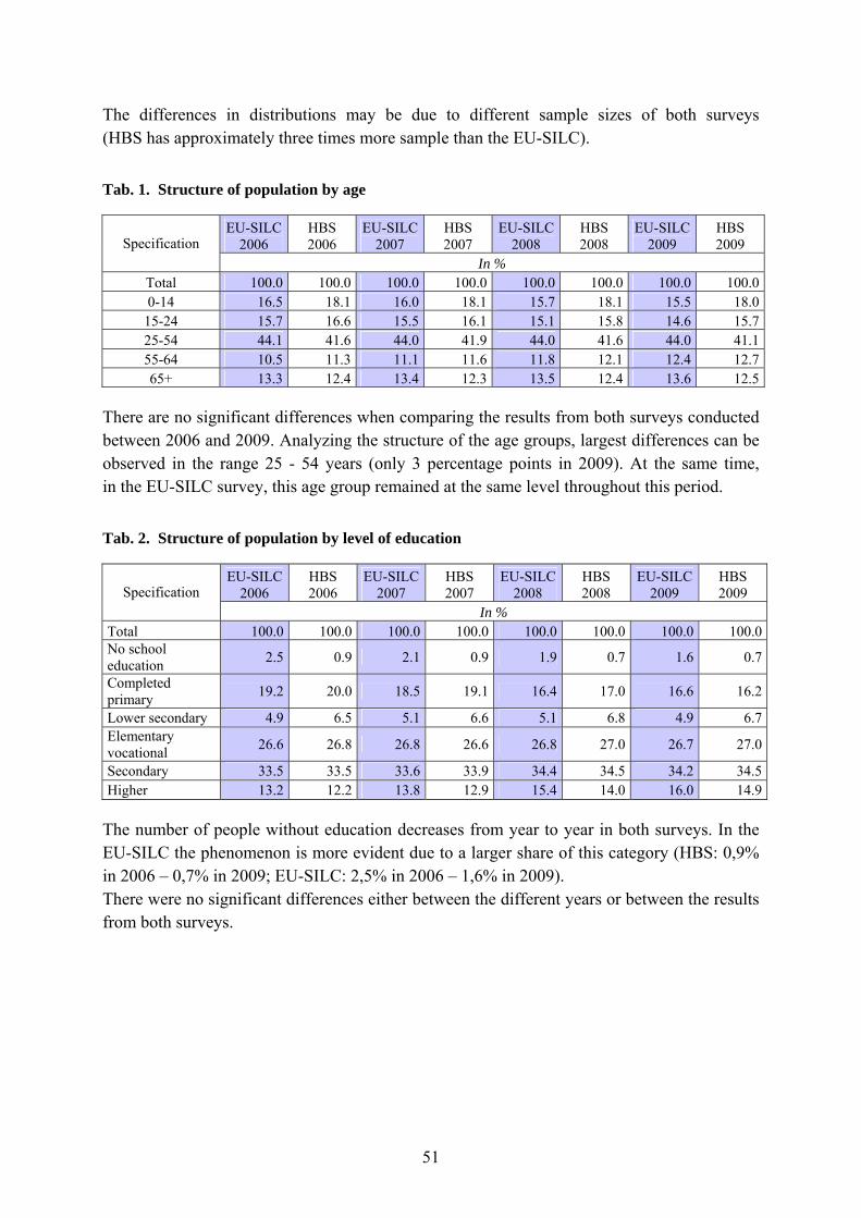
51

The differences in distributions may be due to different sample sizes of both surveys (HBS has approximately three times more sample than the EU-SILC). Tab. 1. Structure of population by age

EU-SILC 2006

HBS 2006

EU-SILC 2007

HBS 2007

EU-SILC 2008

HBS 2008

EU-SILC 2009

HBS 2009 Specification

In % Total 100.0 100.0 100.0 100.0 100.0 100.0 100.0 100.00-14 16.5 18.1 16.0 18.1 15.7 18.1 15.5 18.0

15-24 15.7 16.6 15.5 16.1 15.1 15.8 14.6 15.725-54 44.1 41.6 44.0 41.9 44.0 41.6 44.0 41.155-64 10.5 11.3 11.1 11.6 11.8 12.1 12.4 12.765+ 13.3 12.4 13.4 12.3 13.5 12.4 13.6 12.5

There are no significant differences when comparing the results from both surveys conducted between 2006 and 2009. Analyzing the structure of the age groups, largest differences can be observed in the range 25 - 54 years (only 3 percentage points in 2009). At the same time, in the EU-SILC survey, this age group remained at the same level throughout this period. Tab. 2. Structure of population by level of education

EU-SILC 2006

HBS 2006

EU-SILC 2007

HBS 2007

EU-SILC 2008

HBS 2008

EU-SILC 2009


In % Total 100.0 100.0 100.0 100.0 100.0 100.0 100.0 100.0No school education 2.5 0.9 2.1 0.9 1.9 0.7 1.6 0.7

Completed primary 19.2 20.0 18.5 19.1 16.4 17.0 16.6 16.2

Lower secondary 4.9 6.5 5.1 6.6 5.1 6.8 4.9 6.7Elementary vocational 26.6 26.8 26.8 26.6 26.8 27.0 26.7 27.0

Secondary 33.5 33.5 33.6 33.9 34.4 34.5 34.2 34.5Higher 13.2 12.2 13.8 12.9 15.4 14.0 16.0 14.9

The number of people without education decreases from year to year in both surveys. In the EU-SILC the phenomenon is more evident due to a larger share of this category (HBS: 0,9% in 2006 – 0,7% in 2009; EU-SILC: 2,5% in 2006 – 1,6% in 2009). There were no significant differences either between the different years or between the results from both surveys.

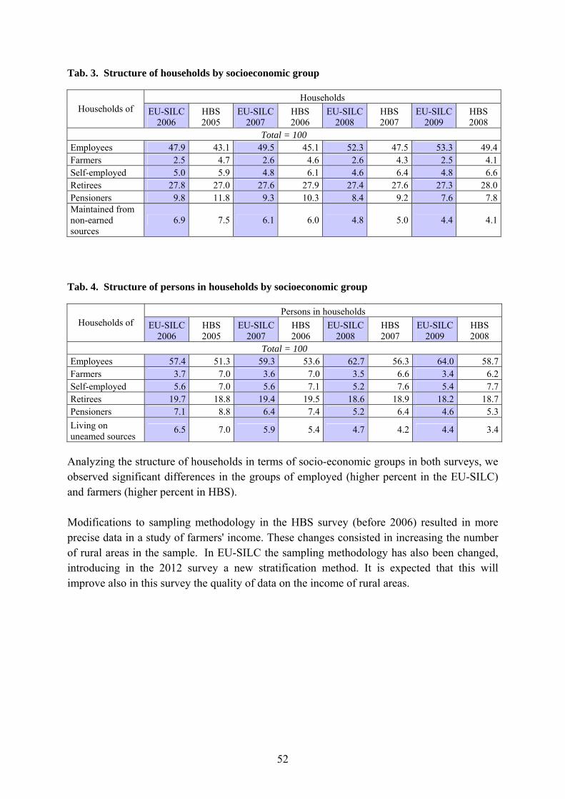
52

Tab. 3. Structure of households by socioeconomic group

Households Households of EU-SILC

2006 HBS 2005

EU-SILC 2007

HBS 2006

EU-SILC 2008

HBS 2007

EU-SILC 2009

HBS 2008

Total = 100 Employees 47.9 43.1 49.5 45.1 52.3 47.5 53.3 49.4Farmers 2.5 4.7 2.6 4.6 2.6 4.3 2.5 4.1Self-employed 5.0 5.9 4.8 6.1 4.6 6.4 4.8 6.6Retirees 27.8 27.0 27.6 27.9 27.4 27.6 27.3 28.0Pensioners 9.8 11.8 9.3 10.3 8.4 9.2 7.6 7.8Maintained from non-earned sources

6.9 7.5 6.1 6.0 4.8 5.0 4.4 4.1

Tab. 4. Structure of persons in households by socioeconomic group

Persons in households Households of EU-SILC

2006 HBS 2005

EU-SILC 2007

HBS 2006

EU-SILC 2008

HBS 2007

EU-SILC 2009

HBS 2008

Total = 100 Employees 57.4 51.3 59.3 53.6 62.7 56.3 64.0 58.7Farmers 3.7 7.0 3.6 7.0 3.5 6.6 3.4 6.2Self-employed 5.6 7.0 5.6 7.1 5.2 7.6 5.4 7.7Retirees 19.7 18.8 19.4 19.5 18.6 18.9 18.2 18.7Pensioners 7.1 8.8 6.4 7.4 5.2 6.4 4.6 5.3Living on uneamed sources

6.5 7.0 5.9 5.4 4.7 4.2 4.4 3.4

Analyzing the structure of households in terms of socio-economic groups in both surveys, we observed significant differences in the groups of employed (higher percent in the EU-SILC) and farmers (higher percent in HBS). Modifications to sampling methodology in the HBS survey (before 2006) resulted in more precise data in a study of farmers' income. These changes consisted in increasing the number of rural areas in the sample. In EU-SILC the sampling methodology has also been changed, introducing in the 2012 survey a new stratification method. It is expected that this will improve also in this survey the quality of data on the income of rural areas.

53

Tab. 5. Average yearly equivalent income in PLN by socio-economic group

Hauseholds of EU-SILC 2006

HBS 2005

EU-SILC 2007

HBS 2006

EU-SILC 2008

HBS 2007

EU-SILC 2009

HBS 2008

Disposable income

Total 14902 13444 16166 14767 18684 16549 21015 18645

Employees 16872 14325 18143 15455 20899 17120 23285 19621

Farmers 9224 12229 10555 13891 13550 16879 13596 17556

Self-employed 18271 18271 17851 20416 21348 23317 26554 24945

Retirees 13700 13309 14668 14278 15618 15089 17209 16445

Pensioners 9649 9622 10880 10478 12061 11472 12930 12104

Living on uneamed sources 7213 8552 8751 9272 9665 10327 11063 11636

Income from hired work

Total 8727 6636 9670 7482 11719 8857 13298 10289

Employees 14160 11695 15236 12677 17609 14287 19520 16053

Farmers 689 1216 1043 1367 1356 1669 1662 1862

Self-employed 2975 2565 2711 2805 3201 3412 4718 3934

Retirees 1270 1266 1467 1423 1545 1694 1746 1823

Pensioners 1004 902 1177 1022 1178 1234 1330 1314

Living on uneamed sources 1390 727 1669 736 2401 936 2581 1134

The most similar results in both surveys were obtained in households of pensioners and retirees. Households dependent on agriculture show higher incomes in the HBS survey than in the EU-SILC. In HBS these incomes include also the value of goods produced for own consumption. Differences in income from employed between surveys arise from the method of data collection. In EU-SILC the annual income date is collected soon after the settlement with the Tax Office and often respondents provide these data on the basis of relevant documents. By contrast, the HBS survey enquires about expenditure and consumption, while income is only additional information. HBS data is collected each month which results in lower availability of evidence of the income. However, in the case of income from agriculture, this method of data collection gives better results.

54

Tab. 6. Average yearly equivalent income in PLN by number of persons

Households with specified number

of persons

EU-SILC 2006

HBS 2005

EU-SILC 2007

HBS 2006

EU-SILC 2008

HBS 2007

EU-SILC 2009

HBS 2008

Disposable income Total 14902 13444 16166 14769 18684 16549 21018 186451 14372 13704 15412 14686 16883 15540 19096 171212 17611 15961 18725 17225 21201 18849 23652 211453 17378 14954 18561 16511 21001 18690 23830 210564 14928 13582 16235 14862 19273 16936 21879 191685 12349 11318 13733 12716 16238 14498 18455 165526 and more 10959 9964 12456 11187 14947 12605 16184 14183

Income from hired work Total 8727 6636 9670 7484 11719 8857 13264 102891 4470 3673 4737 4103 5675 4627 6549 55512 7275 5589 8015 6145 9830 7426 11549 87263 11709 8839 12712 9955 14861 11635 16760 135464 10761 8382 11742 9393 14363 11036 16306 126115 7584 5888 8895 6735 11012 8179 12562 95426 and more 6115 3970 7171 4684 9019 5679 9592 6678

In all the presented years and groups of households, incomes shown in the EU-SILC are higher than in HBS. This results from the previously mentioned methodological differences and method of calculating annual income of the HBS survey (average monthly income multiplied by 12 months). In both surveys there is however a comparable rate of income`s growth over the reported years Tab. 7. Households provided with selected durables

EU-SILC 2006

HBS 2005

EU-SILC 2007

HBS 2006

EU-SILC 2008

HBS 2007

EU-SILC 2009


In % Fixed telephone 74.0 71.9 71.6 67.9 68.5 64.2 64.9 60.7 Mobile telephone 70.7 73.1 75.5 79.3 79.9 83.5 84.1 86.5 Television set 96.9 98.5 97.1 98.5 97.5 98.5 97.8 98.5 Computer 44.4 43.7 48.7 50.1 54.5 56.4 59.3 60.8 Printer 31.8 29.5 35.7 33.6 40.0 37.1 43.9 40.1 Internet connection 28.5 28.4 34.8 36.6 43.0 45.6 51.1 53.4 Microwave oven 34.1 38.0 37.9 42.4 41.9 46.1 46.6 50.1 Dishwasher 8.0 6.2 9.3 7.4 11.5 9.6 13.4 12.3 Refrigerator 96.9 98.6 97.6 98.9 97.7 98.4 98.5 97.9 Washing machine 96.2 96.8 96.6 97.1 96.8 97.3 97.6 97.9 Passenger car 50.7 49.5 53.6 52.5 56.2 54.7 58.9 57.4 Results from both studies are very similar. The greatest differences (about 4 percentage points) are observed in the Telephone and Microwave Oven categories.

55

4.2. Comparison of income data from SNA for the household sector and EU-SILC The comparison covered disposable income and its main components: income from hired employment, self-employment (in and outside farming), as well as social benefits. When comparing these two sources we must take into account some discrepancies. The differences are to a great extent brought about by the methodological diversity. Here are the main diverging points: 1. In SNA the household sector includes collective households which do not enter EU-SILC. 2. Both systems employ different methods of measuring income from self-employment. 3. Accounts of primary and secondary income distribution in SNA used for the determination of disposable income include some items not covered by EU-SILC or not taken into account in the calculation of its results. The most important of them are imputed rents. In SNA income from self-employment is determined as the so called operation surplus which is the balance between the global production and current production inputs (i.e. intermediate consumption) and hired employees’ wages. This difference is reduced by taxes and increased by subsidies. The operation surplus thus calculated is allocated to the household’s consumer needs, housing-related investment as well as production-related investment. In the Polish EU-SILC the question about income from self-employment concerns just the amount allocated to the household’s consumer needs and its housing-related investment. In addition, SNA takes into account consumption from own production which is not taken into consideration by EU-SILC for farmers’ households. Due to these differences incomes from self-employment according to EU-SILC made 24% - 30% of the operation surplus only (after deduction of section K). Incomes from hired employment in EU-SILC 2009 are equal to 101% of the corresponding figure in SNA, while social benefits – 93% respectively, which seems to be a good result. In EU-SILC 2009, as compared with EU-SILC 2006, the data coherence for disposable income with SNA increased by 7 percentage points. This is due to the coherence increase for income from hired employment by 2 percentage points, i.e. from 99% to 101%. In terms of value, wages and other incomes related to hired employment provide the most important component of disposable income in SNA. This category made up over 50% of the disposable income for 2009. In EU-SILC 2008 RB050 weight was used for the calculation of individual incomes, while in EU-SILC 2007 – PB040, respectively. In SNA incomes of the employees working abroad were calculated in a different way. However, these methodological changes do not explain the increased coherence of incomes from hired employment. The change of weight in EU-SILC could justify an increase by 1 percentage point only. The methodological changes of SNA bring about reduced coherence between SNA data and EU-SILC data, since they lead to an increase in wages and other incomes from hired employment in SNA (for 2006 by over PLN

56

15 million). Considering the fact that SNA data are based on the results of the enterprise surveys, it can be judged that the increased coherence of incomes from hired employment might be due to some deterioration of the quality of enterprise survey results in the scope of wages. Unlike for EU-SILC 2006 and 2007, it is less probable that the increased coherence of SNA results in the area of hired employment could be brought about by a higher quality of EU-SILC results, as the coherence for all the other significant economic categories remained more or less at the same level. The data coherence for social benefits between SNA and EU-SILC was 92%, and taking into account the change of the weighting method – 93%, which is equivalent to EU-SILC 2007. The coherence of income from self-employment between EU-SILC 2008 and SNA was 26% and taking into account the change of the weighting method – 27%, which is by 1 percentage point more than in EU-SILC 2007.

Comparison between SNA results for the household sector and EU-SILC

Incomes: 2005 r. Incomes: 2006 r. Incomes: 2007 r. Incomes: 2008 r.

SNA EU-SILC SNA = 100% SNA EU-SILC SNA =

100% SNA EU-SILC SNA EU-SILCCategory in SNA

Category description in

EU-SILC in mln PLN

in mln PLN in mln

PLN in mln PLN in mln

PLN in mln PLN

SNA = 100% in mln

PLN in mln PLN

SNA = 100%

Gross disposable income (net)

Total disposable household income (net)

651 512 369 046 57 683 483 398 939 58 742 374 457 807 62 799 085 513 594 64

Wages, salaries and other income connected with hired work (gross)

Employee cash or near cash income (gross)

303 358 290 140 96 325 030 323 956 99 375 358 380 422 99 426 735 423 255 99

Gross operating surplus (gross) with the exception of section K

Self-employment income (gross) - value allocated to household`s consumption and dwelling-related investment

189 378 50 167 27 201 601 53 219 26 220 168 58 291 26 226 352 67 485 30

Social security benefits and social assistance benefits (gross)

Social benefits (gross) 153 946 141 334 92 161 336 149 258 93 166 880 153 565 93 179 112 163 289 91

Notes:

1. Remarks in brackets: “net” or “gross” refer to including or not including income tax and social security contributions, while the word “gross” in SNA names of categories refers to including fixed assets deppreciation.

2. Data for gross operating surplus in SNA has been taken into consideration with the exception of section K, which allows for better comparability with EU-SILC data on self-employment income (PY050G). The data for section K mainly cover imputed rents, not included in the results of EU-SILC, and market income from renting of real estate included in EU-SILC as variable HY040G.

silc qrfin a pl 2009 0000 v0001 n - europa · comparison of eu-silc and hbs results ... 4 towns 20...

Documents