simatic pcs 7 application note y august 2010 - siemens · pdf filewith pulse width modulation...

Applikationen & Tools

Answers for industry.

Cover

Configurating of Continuous Control with Pulse Width Modulation

SIMATIC PCS 7

Application Note August 2010

2 Continuous Control with Pulse Width Modulation

Version 1.0, Entrys-ID: 44364150

Cop

yrig

ht ©

Sie

men

s A

G 2

010

All

right

s re

serv

ed

Industry Automation and Drives Technologies Service & Support Portal This article is taken from the Service Portal of Siemens AG, Industry Automation and Drives Technologies. The following link takes you directly to the download page of this document. http://support.automation.siemens.com/WW/view/en/44364150 If you have any questions concerning this document please e-mail us to the following address: [email protected]

http://support.automation.siemens.com/WW/view/en/44364150�

mailto:[email protected]�

Continuous Control with Pulse Width Modulation Version 1.0, Entry-ID: 44364150 3

Cop

yrig

ht ©

Sie

men

s A

G 2

010

All

right

s re

serv

ed

s

SIMATIC PCS 7 Continuous Control with Pulse Width Modulation

Indroduction 1

Configuration 2

Simulation Example 3

Conclusion 4

Related Literature 5

History 6

Warranty and Liability



Cop

yrig

ht ©

Sie

men

s A

G 2

010

All

right

s re

serv

ed

Warranty and Liability

Note The Application Examples are not binding and do not claim to be complete regarding the circuits shown, equipping and any eventuality. The Application Examples do not represent customer-specific solutions. They are only intended to provide support for typical applications. You are responsible for ensuring that the described products are used correctly. These application examples do not relieve you of the responsibility to use safe practices in application, installation, operation and maintenance. When using these Application Examples, you recognize that we cannot be made liable for any damage/claims beyond the liability clause described. We reserve the right to make changes to these Application Examples at any time without prior notice. If there are any deviations between the recommendations provided in these application examples and other Siemens publications – e.g. Catalogs – the contents of the other documents have priority.

We do not accept any liability for the information contained in this document.

Any claims against us – based on whatever legal reason – resulting from the use of the examples, information, programs, engineering and performance data etc., described in this Application Example shall be excluded. Such an exclusion shall not apply in the case of mandatory liability, e.g. under the German Product Liability Act (“Produkthaftungsgesetz”), in case of intent, gross negligence, or injury of life, body or health, guarantee for the quality of a product, fraudulent concealment of a deficiency or breach of a condition which goes to the root of the contract (“wesentliche Vertragspflichten”). The damages for a breach of a substantial contractual obligation are, however, limited to the foreseeable damage, typical for the type of contract, except in the event of intent or gross negligence or injury to life, body or health. The above provisions do not imply a change of the burden of proof to your detriment. Any form of duplication or distribution of these Application Examples or excerpts hereof is prohibited without the expressed consent of Siemens Industry Sector.

Preface


Cop

yrig

ht ©

Sie

men

s A

G 2

010

All

right

s re

serv

ed

4436

4150

_Pul

se_W

idth

_Mod

ulat

ion_

en.d

oc

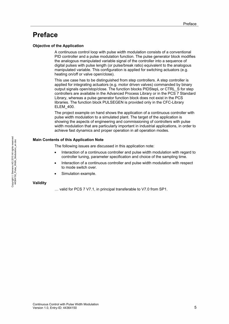
Preface Objective of the Application

A continuous control loop with pulse width modulation consists of a conventional PID controller and a pulse modulation function. The pulse generator block modifies the analogous manipulated variable signal of the controller into a sequence of digital pulses with pulse length (or pulse/break ratio) equivalent to the analogous manipulated variable. This configuration is applied for switching actuators (e.g. heating on/off or valve open/close). This use case has to be distinguished from step controllers. A step controller is applied for integrating actuators (e.g. motor driven valves) commanded by binary output signals open/stop/close. The function blocks PIDStepL or CTRL_S for step controllers are available in the Advanced Process Library or in the PCS 7 Standard Library, whereas a pulse generator function block does not exist in the PCS libraries. The function block PULSEGEN is provided only in the CFC-Library ELEM_400. The project example on hand shows the application of a continuous controller with pulse width modulation to a simulated plant. The target of the application is showing the aspects of engineering and commissioning of controllers with pulse width modulation that are particularly important in industrial applications, in order to achieve fast dynamics and proper operation in all operation modes.

Main Contents of this Application Note The following issues are discussed in this application note: • Interaction of a continuous controller and pulse width modulation with regard to

controller tuning, parameter specification and choice of the sampling time. • Interaction of a continuous controller and pulse width modulation with respect

to mode switch over. • Simulation example.

Validity … valid for PCS 7 V7.1, in principal transferable to V7.0 from SP1.

http://dict.leo.org/ende?lp=ende&p=Ci4HO3kMAA&search=continuous&trestr=0x8004�

Table of Contents



Cop

yrig

ht ©

Sie

men

s A

G 2

010

All

right

s re

serv

ed

Table of Contents Warranty and Liability ................................................................................................. 4 Preface .......................................................................................................................... 5 1 Introduction........................................................................................................ 7

1.1 Basic Principles of Control with Pulse Width Modulation..................... 7 1.2 Sample Rates, Pulse Time and Control Precision ............................... 9 1.3 Application Examples........................................................................... 9 1.3.1 Two-step Control with Unipolar MV Range (0% ... +100%)................. 9 1.3.2 Three-step Control with Two Binary Actuators .................................... 9 1.3.3 Two-step Controller with Bipolar MV Range (-100% ... +100%)........ 10

2 Configuration ................................................................................................... 11 2.1 Creating an Instance of the Process Tag Type.................................. 11 2.2 Insert the Pulse Width Modulation Block............................................ 12 2.3 Simulation for Controllers with Pulse Width Modulation .................... 16 2.4 Two-step or Three-step Control ......................................................... 16 2.5 Synchronization of Controller and Pulse Generator Block................. 16 2.6 Parameterization and Controller settings ........................................... 17 2.7 Control Performance Monitoring ........................................................ 18

3 Simulation Example......................................................................................... 19 4 Conclusion ....................................................................................................... 22 5 Related Literature ............................................................................................ 23 6 History............................................................................................................... 24

1 Introduction1.1 Basic Principles of Control with Pulse Width Modulation


Cop

yrig

ht ©

Sie

men

s A

G 2

010

All

right

s re

serv

ed

1 Introduction

1.1 Basic Principles of Control with Pulse Width Modulation

A continuous control with pulse width modulation consists of a controller (e.g. PID-controller) whose manipulated variable is an analogous value (e.g. 0….100%) and a downstream pulse width modulation which generates a sequence of binary pulses (e.g. on/off) from the continuous manipulated variable. This type of the controllers is used for switching actuators e.g. for the temperature control of a boiler with a burner which can be only turned on or off.

The pulse time (relative to the total time period of pulse and pause time) is proportional to the analogous manipulated variable. Examples:

• Manipulated variable 100% means permanent impulse, i.e. always “on”, or maximum heating power.

• Manipulated variable 50%: For the half of a defined time period the signal is „on“ and for the other half time the signal is “off”, i.e. half heating power in temporal average.

PID

controller

pulse widthmodulation

controlled system

setpoint

processvariable

+ - PID

controller

pulse widthmodulation

controlled system

setpoint

processvariable

+ -

Figure 1-1: Signal flow scheme of a control loop with pulse width modulation

1 Introduction 1.1 Basic Principles of Control with Pulse Width Modulation



Cop

yrig

ht ©

Sie

men

s A

G 2

010

All

right

s re

serv

ed

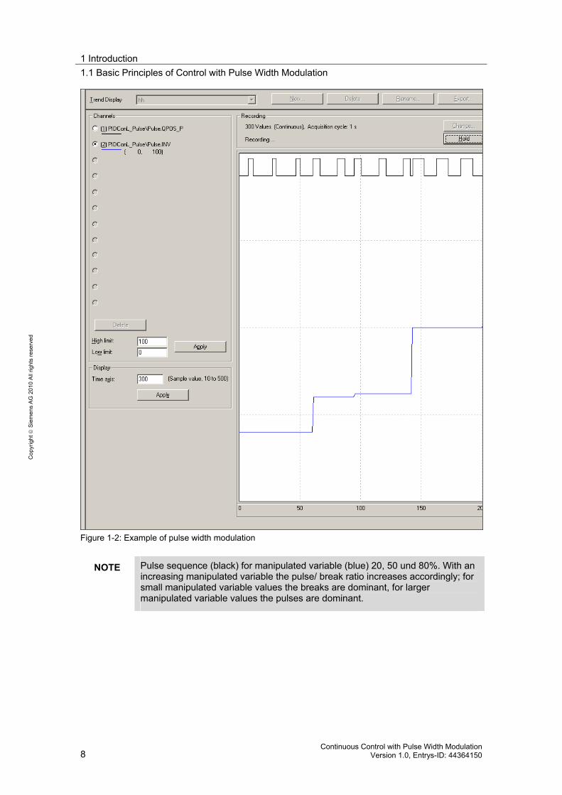
Figure 1-2: Example of pulse width modulation

NOTE Pulse sequence (black) for manipulated variable (blue) 20, 50 und 80%. With an increasing manipulated variable the pulse/ break ratio increases accordingly; for small manipulated variable values the breaks are dominant, for larger manipulated variable values the pulses are dominant.

1 Introduction1.2 Sample Rates, Pulse Time and Control Precision


Cop

yrig

ht ©

Sie

men

s A

G 2

010

All

right

s re

serv

ed

1.2 Sample Rates, Pulse Time and Control Precision

The controller calculates a suitable manipulated variable at every sample time. These manipulated variable values are converted by the pulse generator into impulses with a specified width. Therefore it makes sense to calculate a new manipulated variable only after the time of the maximum pulse length (pulse period time) has passed. To reach a good resolution of the pulse duration (with respect to amplitude quantization), the sample rate of the pulse generator must be much smaller than that one of the controller.

Example The sample time of the controller is fixed to 5s, the maximum pulse width (pulse period time) is therefore 5s. If the pulse generator is running with a sample time of 0.5s the pulse width can be determined in a grid of 0.5s mesh size, which means in 10% steps of the manipulated variable. If the pulse width modulator is executed in a cycle of 0.1s, the resolution is 2%.

This amplitude quantization (resolution) of the manipulated variable has consequences for the feasible control precision. Only stationary process values which fall into the manipulated variable grid multiplied with the controlled system gain can be reached exactly. Assuming a controlled system gain of 5°C/% in the above example this would be a grid resolution of:

2% * 5°C/%=10°C.

Setpoints which do not fit into this grid cannot be reached precisely and therefore a continuous oscillation of the process variable around the setpoint occurs. In case of relaxed requirements with respect to control precision the oscillation can be prevented by a dead band around the setpoint. The dead band must be large enough such that the process value can find a value of its grid steps within the dead zone. In the example a dead band of ±5° degrees Celsius would be necessary. If the dead band is smaller, a continuous oscillation around the dead band arises.

1.3 Application Examples

Different classes of application examples can be distinguishing depending on the direction of action of the actuator (or the actuators).

1.3.1 Two-step Control with Unipolar MV Range (0% ... +100%)

• Temperature control with gas burner on/off • Temperature control with electrical heating on/off (by contactor or semi-

conductor relay) • Flow control with switching valve open/close or pump on/off Generally, you will find binary actuator devices like electrical heatings or switching valves in smaller plants e.g. in the laboratory area, in bio process engineering (fermenter) or in the pharmaceutical industry. Switching valves are not common for larger pipe diameters, and larger units (reactors or columns) are rather heated with steam than with electricity.

1.3.2 Three-step Control with Two Binary Actuators

• Temperature control with heating (e.g. electrical heating on/off) and cooling (e.g. switching valve for cooling water inlet open/close or cooling fan on/off)

1 Introduction 1.3 Application Examples



Cop

yrig

ht ©

Sie

men

s A

G 2

010

All

right

s re

serv

ed

• pH-value control with two switching valves open/close for the feed of acid and base

• Pressure control with two switching valves open/close for the gas inlet (e.g. inert gas) and purge outlet of the unit.

In these cases the pulse generator includes the function of a split-range block that splits the manipulated variable of the controller into two actuators with opposite direction of action.

Figure 1-3: PCS 7 automation of a fermenter for recombinated proteins for vaccine production.

NOTE Both the pH-value control QIC300 and the temperature control TIC500 work as three-step controllers with pulse width modulation.

1.3.3 Two-step Controller with Bipolar MV Range (-100% ... +100%)

This configuration makes only sense if there is a binary actuator whose output signal TRUE takes a physical effect into one direction, and the output signal FALSE takes a physical effect in the opposite direction. This means that the controller does not have any possibility of really forwarding the MV value zero to the process. Although the function block PULSGEN provides this possibility, it is rarely used in practice.

http://dict.leo.org/ende?lp=ende&p=Ci4HO3kMAA&search=direction&trestr=0x801�

http://dict.leo.org/ende?lp=ende&p=Ci4HO3kMAA&search=of&trestr=0x801�

http://dict.leo.org/ende?lp=ende&p=Ci4HO3kMAA&search=action&trestr=0x801�

2 Configuration2.1 Creating an Instance of the Process Tag Type


Cop

yrig

ht ©

Sie

men

s A

G 2

010

All

right

s re

serv

ed

2 Configuration If you implement a new continuous control with pulse width modulation in your project, it is recommended start with a process tag type of a continuous controller e.g. “PIDConL_ConPerMon" from the Advanced Process Library.

2.1 Creating an Instance of the Process Tag Type

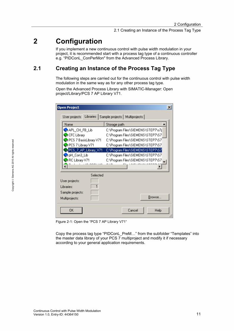
The following steps are carried out for the continuous control with pulse width modulation in the same way as for any other process tag type. Open the Advanced Process Library with SIMATIC-Manager: Open project/Library/PCS 7 AP Library V71.

Figure 2-1: Open the “PCS 7 AP Library V71“

Copy the process tag type “PIDConL_PreM…” from the subfolder “Templates” into the master data library of your PCS 7 multiproject and modify it if necessary according to your general application requirements.



2 Configuration 2.2 Insert the Pulse Width Modulation Block



Cop

yrig

ht ©

Sie

men

s A

G 2

010

All

right

s re

serv

ed

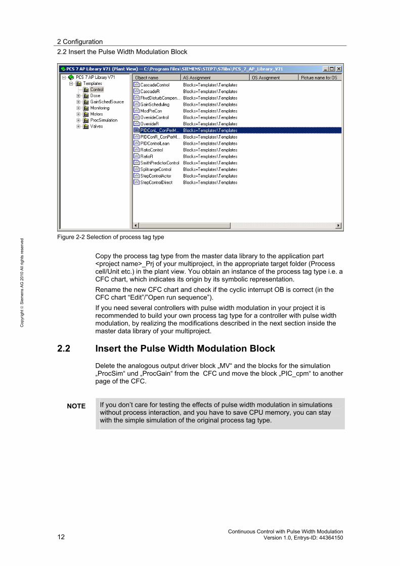
Figure 2-2 Selection of process tag type

Copy the process tag type from the master data library to the application part <project name>_Prj of your multiproject, in the appropriate target folder (Process cell/Unit etc.) in the plant view. You obtain an instance of the process tag type i.e. a CFC chart, which indicates its origin by its symbolic representation. Rename the new CFC chart and check if the cyclic interrupt OB is correct (in the CFC chart “Edit”/”Open run sequence”). If you need several controllers with pulse width modulation in your project it is recommended to build your own process tag type for a controller with pulse width modulation, by realizing the modifications described in the next section inside the master data library of your multiproject.

2.2 Insert the Pulse Width Modulation Block

Delete the analogous output driver block „MV“ and the blocks for the simulation „ProcSim“ und „ProcGain“ from the CFC und move the block „PIC_cpm“ to another page of the CFC.

NOTE If you don’t care for testing the effects of pulse width modulation in simulations without process interaction, and you have to save CPU memory, you can stay with the simple simulation of the original process tag type.

2 Configuration2.2 Insert the Pulse Width Modulation Block


Cop

yrig

ht ©

Sie

men

s A

G 2

010

All

right

s re

serv

ed

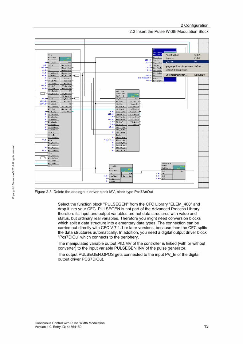
Figure 2-3: Delete the analogous driver block MV, block type Pcs7AnOut

Select the function block "PULSEGEN" from the CFC Library "ELEM_400" and drop it into your CFC. PULSEGEN is not part of the Advanced Process Library, therefore its input and output variables are not data structures with value and status, but ordinary real variables. Therefore you might need conversion blocks which split a data structure into elementary data types. The connection can be carried out directly with CFC V 7.1.1 or later versions, because then the CFC splits the data structures automatically. In addition, you need a digital output driver block "Pcs7DiOu" which connects to the periphery. The manipulated variable output PID.MV of the controller is linked (with or without converter) to the input variable PULSEGEN.INV of the pulse generator. The output PULSEGEN.QPOS gets connected to the input PV_In of the digital output driver PCS7DiOut.

2 Configuration 2.2 Insert the Pulse Width Modulation Block



Cop

yrig

ht ©

Sie

men

s A

G 2

010

All

right

s re

serv

ed

Figure 2-4: Selection of the pulse generator function block „PULSEGEN“ from the CFC Library

„ELEM_400”

2 Configuration2.2 Insert the Pulse Width Modulation Block


Cop

yrig

ht ©

Sie

men

s A

G 2

010

All

right

s re

serv

ed

Figure 2-5: CFC-chart with pulse width modulation and simulation of the controlled system

2 Configuration 2.3 Simulation for Controllers with Pulse Width Modulation



Cop

yrig

ht ©

Sie

men

s A

G 2

010

All

right

s re

serv

ed

NOTE You see that the blocks are located in different cyclic tasks (OB32, OB35), c.f. section 2.6

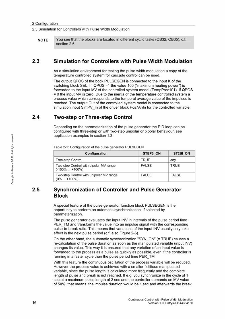
2.3 Simulation for Controllers with Pulse Width Modulation

As a simulation environment for testing the pulse width modulation a copy of the temperature controlled system for cascade control can be used. The output QPOS of the bock PULSEGEN is connected to the input K of the switching block SEL. If QPOS =1 the value 100 ("maximum heating power") is forwarded to the input MV of the controlled system model (TempProc101). If QPOS = 0 the input MV is zero. Due to the inertia of the temperature controlled system a process value which corresponds to the temporal average value of the impulses is reached. The output Out of the controlled system model is connected to the simulation input SimPV_In of the driver block Pcs7AnIn for the controlled variable.

2.4 Two-step or Three-step Control

Depending on the parameterization of the pulse generator the PID loop can be configured with three-step or with two-step unipolar or bipolar behaviour, see application examples in section 1.3. Table 2-1: Configuration of the pulse generator PULSEGEN

Configuration STEP3_ON ST2BI_ON

Tree-step Control TRUE any Two-step Control with bipolar MV range (-100% ... +100%)

FALSE TRUE

Two-step Control with unipolar MV range (0% ... +100%)

FALSE FALSE

2.5 Synchronization of Controller and Pulse Generator Block

A special feature of the pulse generator function block PULSEGEN is the opportunity to perform an automatic synchronization, if selected by parameterization. The pulse generator evaluates the input INV in intervals of the pulse period time PER_TM and transforms the value into an impulse signal with the corresponding pulse-to-break ratio. This means that variations of the input INV usually only take effect in the next pulse period (c.f. also Figure 2-6). On the other hand, the automatic synchronization "SYN_ON" (= TRUE) causes a re-calculation of the pulse duration as soon as the manipulated variable (input INV) changes its value. This way it is ensured that any variation of an input value is forwarded to the process as a pulse as quickly as possible, even if the controller is running in a faster cycle than the pulse period time PER_TM. With this feature the continuous oscillation of the process variable will be reduced. However the process value is achieved with a smaller fictitious manipulated variable, since the pulse length is calculated more frequently and the complete length of pulse and break is not reached. If e.g. you synchronize in the cycle of 1 sec at a maximum pulse length of 2 sec and the controller demands an MV value of 50%, that means the impulse duration would be 1 sec and afterwards the break

2 Configuration2.6 Parameterization and Controller settings


Cop

yrig

ht ©

Sie

men

s A

G 2

010

All

right

s re

serv

ed

would be 1 sec, too. Due to the new synchronization after 1 sec, the break cannot be kept because the pulse length is re-calculated and forwarded again now. The process variable is getting larger therefore and the controller fights against it, commanding a smaller manipulated variable. The constant pulse period time and therefore the reproducible relationship between analogous manipulated variable and pulse/break ratio is lost. The disadvantage comes to light when the controller is switched from automatic mode to manual mode keeping the last MV value constant. Since the manipulated variable does not change its value any more there is no new synchronization and the original pulse period is active again. The consequence is that the actual value runs away. Therefore the automatic synchronization should normally remain switched off (input "SYN_ON" = FALSE) to guarantee the clear interpretability of the analogous manipulated variable and the correct function of the manual/automatic mode switchover.

2.6 Parameterization and Controller settings

QPOS_P

P_B_TM

PER_TM

SampleTime Figure 2-6: Cycles of pulse generator operation.

NOTE Binary output signal QPOS_P, minimum pulse/break time P_B_TM, pulse period time PER_TM. The controller cycle SampleTime is double frequency compared to pulse period time in that example.

Parameterize the pulse generator first and then the controller.

• The minimum pulse/break time P_B_TM corresponds to the speed of the actuator. It must be long enough such that a pulse of minimal length can actually be realized by the actuator (and the digital periphery). For semi-conductor relays minimum pulse times of milliseconds are feasible while for switching valves the minimum pulse times are in the order of seconds, depending on pipe diameter.

• The cycle time of the pulse generator and all down stream function blocks must be less or equal to the minimum pulse/break time, such that pulses of minimal length can really be created and forwarded to the process. Please move the respective function blocks into the suitable OB-Cycle in the CFC.

• Set the pulse period time PER_TM larger than the minimum pulse/break time at least by a factor of 20 (for 5% quantization of the manipulated variable) until a factor of 100 (for 1% quantization of the manipulated variable).

2 Configuration 2.7 Control Performance Monitoring



Cop

yrig

ht ©

Sie

men

s A

G 2

010

All

right

s re

serv

ed

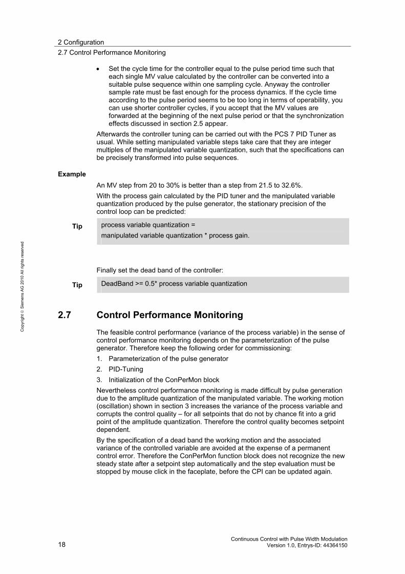
• Set the cycle time for the controller equal to the pulse period time such that each single MV value calculated by the controller can be converted into a suitable pulse sequence within one sampling cycle. Anyway the controller sample rate must be fast enough for the process dynamics. If the cycle time according to the pulse period seems to be too long in terms of operability, you can use shorter controller cycles, if you accept that the MV values are forwarded at the beginning of the next pulse period or that the synchronization effects discussed in section 2.5 appear.

Afterwards the controller tuning can be carried out with the PCS 7 PID Tuner as usual. While setting manipulated variable steps take care that they are integer multiples of the manipulated variable quantization, such that the specifications can be precisely transformed into pulse sequences.

Example An MV step from 20 to 30% is better than a step from 21.5 to 32.6%. With the process gain calculated by the PID tuner and the manipulated variable quantization produced by the pulse generator, the stationary precision of the control loop can be predicted:

Tip process variable quantization = manipulated variable quantization * process gain.

Finally set the dead band of the controller:

Tip DeadBand >= 0.5* process variable quantization

2.7 Control Performance Monitoring

The feasible control performance (variance of the process variable) in the sense of control performance monitoring depends on the parameterization of the pulse generator. Therefore keep the following order for commissioning: 1. Parameterization of the pulse generator 2. PID-Tuning 3. Initialization of the ConPerMon block Nevertheless control performance monitoring is made difficult by pulse generation due to the amplitude quantization of the manipulated variable. The working motion (oscillation) shown in section 3 increases the variance of the process variable and corrupts the control quality – for all setpoints that do not by chance fit into a grid point of the amplitude quantization. Therefore the control quality becomes setpoint dependent. By the specification of a dead band the working motion and the associated variance of the controlled variable are avoided at the expense of a permanent control error. Therefore the ConPerMon function block does not recognize the new steady state after a setpoint step automatically and the step evaluation must be stopped by mouse click in the faceplate, before the CPI can be updated again.

http://dict.leo.org/ende?lp=ende&p=Ci4HO3kMAA&search=operability&trestr=0x801�

http://dict.leo.org/ende?lp=ende&p=Ci4HO3kMAA&search=associated&trestr=0x8004�

3 Simulation Example


Cop

yrig

ht ©

Sie

men

s A

G 2

010

All

right

s re

serv

ed

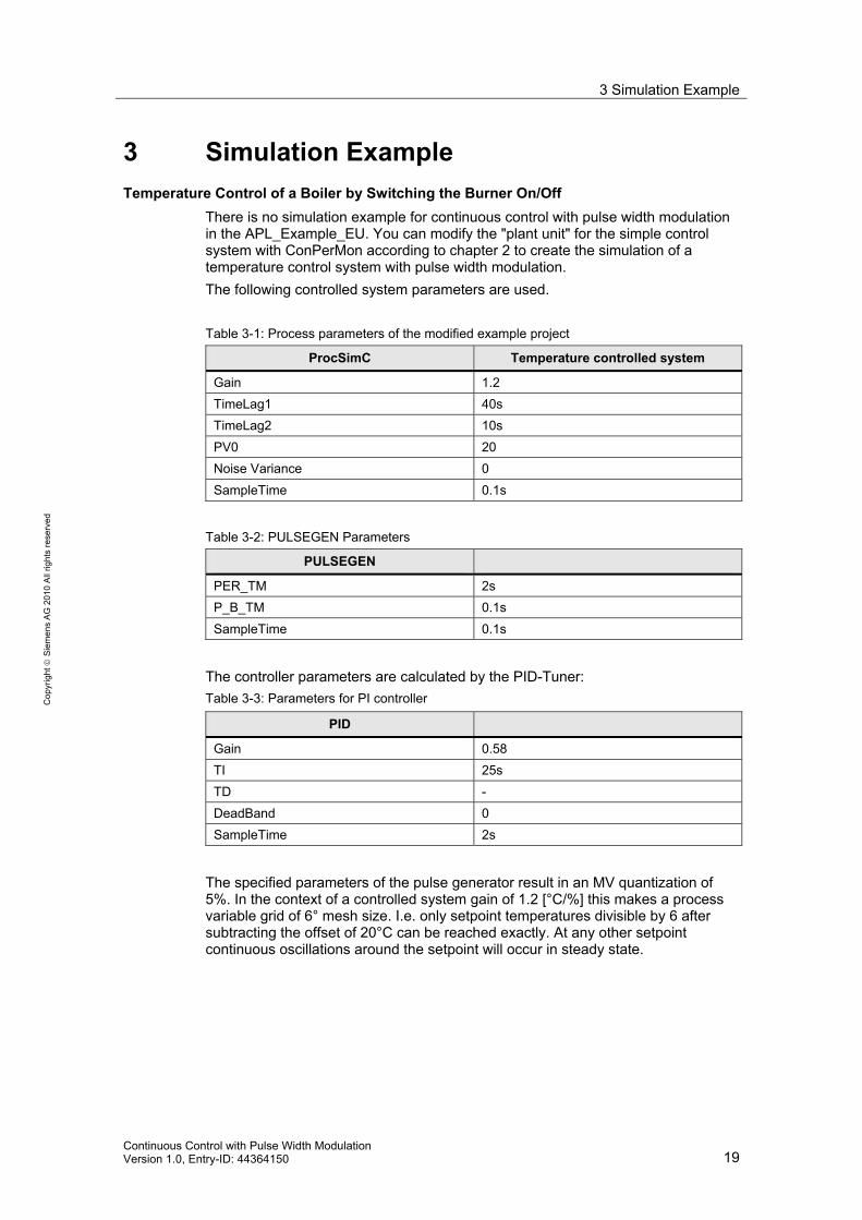
3 Simulation Example Temperature Control of a Boiler by Switching the Burner On/Off

There is no simulation example for continuous control with pulse width modulation in the APL_Example_EU. You can modify the "plant unit" for the simple control system with ConPerMon according to chapter 2 to create the simulation of a temperature control system with pulse width modulation. The following controlled system parameters are used. Table 3-1: Process parameters of the modified example project

ProcSimC Temperature controlled system

Gain 1.2 TimeLag1 40s TimeLag2 10s PV0 20 Noise Variance 0 SampleTime 0.1s

Table 3-2: PULSEGEN Parameters

PULSEGEN

PER_TM 2s P_B_TM 0.1s SampleTime 0.1s

The controller parameters are calculated by the PID-Tuner: Table 3-3: Parameters for PI controller

PID

Gain 0.58 TI 25s TD - DeadBand 0 SampleTime 2s

The specified parameters of the pulse generator result in an MV quantization of 5%. In the context of a controlled system gain of 1.2 [°C/%] this makes a process variable grid of 6° mesh size. I.e. only setpoint temperatures divisible by 6 after subtracting the offset of 20°C can be reached exactly. At any other setpoint continuous oscillations around the setpoint will occur in steady state.




Cop

yrig

ht ©

Sie

men

s A

G 2

010

All

right

s re

serv

ed

Figure 3-1: Small continuous oscillation around the setpoint 40° C

The continuous oscillation around the set-point can be prevented by the activation of a dead band. In this example a dead band of ±3°C degrees must be chosen such that it has a width of 6°. The process value then settles at a steady state exactly at this grid point which lies within the dead band, i.e. the actual value does not reach the setpoint exactly.



Cop

yrig

ht ©

Sie

men

s A

G 2

010

All

right

s re

serv

ed

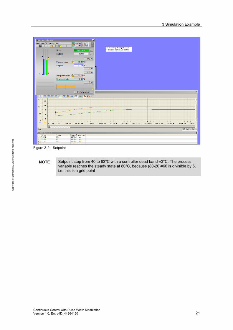
Figure 3-2: Setpoint

NOTE Setpoint step from 40 to 83°C with a controller dead band ±3°C. The process variable reaches the steady state at 80°C, because (80-20)=60 is divisible by 6, i.e. this is a grid point

http://dict.leo.org/ende?lp=ende&p=Ci4HO3kMAA&search=divisible&trestr=0x8004�

http://dict.leo.org/ende?lp=ende&p=Ci4HO3kMAA&search=by&trestr=0x8004�

4 Conclusion



Cop

yrig

ht ©

Sie

men

s A

G 2

010

All

right

s re

serv

ed

4 Conclusion Controllers with pulse width modulation are suitable for systems with switching actuators. Although there is no pulse generator block in the PCS 7 libraries, the PULSEGEN block from the CFC-Library ELEM_400 can be used. You must find a compromise between the stationary precision of a control loop and the pulse period time at given minimum pulse/break time. A long pulse period time means high accuracy but accordingly slow controller sample time. Shorter pulse period times reduce control precision due to the coarse manipulated variable quantization and require adequate wide dead bands of the controller. The combination of pulse generator and digital output driver replaces the analogous output driver of the controller, independently of the kind of controller type that is used. A pulse generator can therefore be connected to a predictive controller (MPC) just as well as to a PID controller, and is also compatible with extended PID structures (e.g. Gain scheduling, Override, disturbance variable feed-forward, ratio control). A split range function can be connected to any continuous controller to split the manipulated variable of the controller into two actuators with an opposite direction of action. If the actuators are binary actors, the function block PULSEGEN also includes a split range function.

Special Cases • In cascade control loops the pulse generator is of course only relevant for the

slave controller. • In a Smith predictor the controller internal process model should be supplied

with the analogous output signal of the controller block. The analogous output signal of the controller is also used by the MPC configurator for modelling from learning data such that the behaviour of the process incl. pulse generator is identified and mapped into the model.

http://dict.leo.org/ende?lp=ende&p=Ci4HO3kMAA&search=accuracy&trestr=0x2801�

5 Related Literature


Cop

yrig

ht ©

Sie

men

s A

G 2

010

All

right

s re

serv

ed

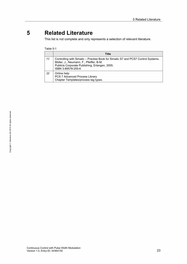
5 Related Literature This list is not complete and only represents a selection of relevant literature. Table 5-1

Title

/1/ Controlling with Simatic – Practise Book for Simatic S7 and PCS7 Control Systems. Müller, J., Neumann, F., Pfeiffer, B-M. Publicis Corporate Publishing, Erlangen, 2005. ISBN 3-89578-255-6

/2/ Online help PCS 7 Advanced Process Library Chapter Templates/process tag types.

6 History



Cop

yrig

ht ©

Sie

men

s A

G 2

010

All

right

s re

serv

ed

6 History Table 6-1

Version Date Modifications

V1.0 August 2010 First version

simatic pcs 7 application note y august 2010 - siemens · pdf filewith pulse width modulation...

Documents