arX

iv:0

911.

2012

v2 [

phys

ics.

chem

-ph]

15

May

201

2

Simple isotherm equations to fit type I adsorption

data

Martın A. Mosquera

Department of ChemistryPurdue University, 560 Oval Drive, West Lafayette, IN 47907, USA

mmosquer@purdue.edu

May 16, 2012

Abstract

A simple model to fit experimental data of adsorption of gases andvapours on microporous adsorbents (type I isotherms) is proposed. Themain assumption is that the adsorbate phase can be divided into identicaland non-interacting effective subsystems. This gives rise to a simple mul-tiparametric isotherm based on the grand canonical ensemble statistics,whose functional form is a ratio of two polynomial functions. The pa-rameters are interpreted as effective equilibrium constants. A simplifiedisotherm that reduces the number of adjustable parameters with respectto the general isotherm is also proposed. We show how to use theseisotherms to fit the adsorption data in such way that the parameters havestatistical significance. Due to their high accuracy, both isotherms canbe used to estimate thermodynamic properties like isosteric and differen-tial heats of adsorption. A simple method is presented for systems thatshow an apparent variation in the coverage limit with temperature. Thismethod avoids overparametrization and improves fitting deviations. Fi-nally, several applications to fitting data, taken from the literature, ofadsorption of some gases on activated carbon, molecular sieving carbon,silica gel, and pillared clays are presented.

1 Introduction

Correlating adsorption data obtained from experiments or computer calcula-tions is necessary to save time and efforts in additional experimentation orcomputing time. Because of the complexity of the equilibrium adsorption phe-nomenon, the research of new models of adsorption is still very active. A goodparameter-adjustable model must fit well the experimental data and predictthermodynamic quantities correctly; therefore, it is necessary to analyse themodel and assess its capabilities. Many industrial applications of adsorptionencompass a wide range of adsorbent saturation. Thus, models which offer

1

the experimentalist and process engineer the possibility to set the number ofadjustable parameters are required.

Many adsorbents used in industry and research present certain degree of het-erogeneity in terms of pore size distribution and surface topography. Dependingon each of these factors, different isotherm models are proposed. For example,lattice gas theories which simplify the structure of the adsorbent surface bytaking into account only the most important adsorption sites of the adsorbentsurface or adsorption pores have been developed. Many of these theories are con-sistent with experiments and computer simulations [1, 2, 16, 23–25, 27–30, 39].A disadvantage of this kind of models is that many gas-solid systems presentunique characteristics. Thus, they may not be applicable if some assumptionsor conditions are violated.

Another commonly used method to obtain isotherms for heterogeneous sys-tems is the integration over a patchwise topography of adsorption sites [10].Modified isotherms arise by assuming an adsorption energy distribution func-tion and an ideal local isotherm like the Langmuir equations. Even thoughsome of these equations work well for a large number of systems, they presentlimitations associated with the assumptions of the particular model, e.g., somemodels do not provide the correct Henry’s law limit. Moreover, this integrationmethod is somewhat difficult because the complexity of the adsorption energydistribution makes it difficult to obtain the analytical expression for the trans-formed isotherm. The equations of Sips [35], Toth [40], and UNILAN [36] arethe most widely used isotherms of this type.

In this work simplified isotherms to fit type I adsorption data are proposed.The model to derive the isotherms is the cell model of adsorption shown by Hill[12–14], which is based on the grand canonical ensemble statistics. The generalisotherm that arises from the cell model has been quite successful to fit exper-imental data of adsorption of gases on zeolites [3, 7, 8, 31–33, 38]. Recently,we showed how to employ this model to fit isotherms of adsorption of gasesand vapours on zeolites [22] and that the parameters could be interpreted asadsorption equilibrium constants. Further validation of this generalized statisti-cal thermodynamical adsorption (GSTA) model has been shown with excellentresults for both adsorption data and thermodynamic properties [20, 21]. Here,we present an accurate extension of the GSTA model and a new simplifiedisotherm is derived from it. It is shown that these isotherm equations can beused to fit type I experimental adsorption isotherms and predict thermodynamicproperties. To illustrate this idea, several experimental adsorption isotherms arecorrectly fitted with these isotherms. Furthermore, extrapolations to tempera-tures beyond the experimental temperature range are possible. Because of thecomplexity of heterogeneous adsorbents, it is suggested that the method pre-sented here is semi-empirical and the cells ensemble can be considered as aneffective grand ensemble of small subsystems.

2

2 Theory

2.1 The general adsorption isotherm

Consider a single-component gas in equilibrium with an adsorbate phase andsuppose that the adsorbate phase can be divided into M identical cells that arenot interacting in the ensemble picture. This means that they are coupled bya very small interaction such that the exchange of molecules in between cellstakes place in a time scale which is large in comparison with the characteristictime scales of the fundamental molecular processes that occur inside each cell.The total number of cells is temperature-independent and the cell volume aswell. It is plausible to assume that a maximum of ns molecules can adsorb onthe subsystem, i.e. the adsorbent has a saturation limit. Under these assump-tions we can express the grand canonical partition function Ξ as a product ofsubsystem’s partition functions [14]:

Ξ = ξM (1)

where

ξ = 1 +

ns∑

j=1

Kjaj (2)

and a is the activity of the system:

a =f

P 0(3)

Since we are concerned with the low pressure regime then a = P/P 0. Theequilibrium constant Kj is expressed as

Kj(T ) = exp( jµ0

g −ASj

kBT

)

(4)

where µ0 is the chemical potential of the gas at the reference pressure P 0 andAS

j is a microscopic free energy which can be written in terms of the partitionfunction of the subsystem with j molecules and volume vS (QS(T, vS , j)):

ASj = −kBT lnQS(T, vS , j) (5)

Now the saturation of the system (q) is simply:

q =qmns

ns∑

j=1

jKjaj

1 +

ns∑

j=1

Kjaj

(6)

Based on its definition, the term Kj can be regarded as an adsorption equilib-rium constant [22]. Therefore, in analogy with chemical equilibrium constants,

3

we can propose the following relation:

lnKj = lnK◦

j −∆hj

RT(7)

where lnK◦

j and ∆hj are the change of entropy and enthalpy, respectively. Theyare related with the adsorption of j molecules onto a representative microscopicsubsystem at the reference pressure P 0. In his seminal paper, the Eq. (6) wasalso derived by Langmuir [18] using chemical kinetics for the case in which a sitecan hold several molecules and the adsorbent is composed by non-interactingsites. In light of his proposal, the term Kj is partitioned as follows:

Kj =1

j!

j∏

i=1

Ri (8)

In a similar fashion, Rj obeys the following relation:

Rj = R◦

j exp(−∆hj

RT

)

(9)

where

R◦

j =jK◦

j

K◦

j−1

(10)

∆hj = ∆hj − ∆hj−1 (11)

In order to fit an isotherm at constant temperature using Eq. (6), the adjustableparameters are {Rj} instead of {Kj}. For the case in which several isothermsat different temperatures have been measured, the adjustable parameters are{lnR◦

j}, {∆hj}, and qm. Hence, a total of 2ns + 1 parameters are required.The present model suggests that ξ → Ξ as the subsystem volume is in-

creased. Thus, in order to predict q we should assume that the maximum num-ber of molecules ns and the volume vS are very large. However if we assumethat each Rj is an adjustable parameter, then this would give us a large numberof adjustable parameters with poor statistical confidence [33]. A solution to thisproblem is to assume ns as a small number of molecules that adsorb into a mi-croscopic imaginary effective subsystem, and the parameters {Rj} as represen-tative parameters of the experimental adsorption isotherm. The characteristicsof the adsorbate+adsorbent system like molecule-surface and molecule-moleculeinteractions are included effectively in these subsystems; probably by a modi-fied intermolecular potential. This is ad hoc guess is a convenient picture thatallows us to apply the cell model to complex zeolite and heterogeneous systemsin general.

The probability that a subsystem with j adsorbed molecules will be foundis (assuming ideal gas phase):

pj =Kja

j

ξ(12)

4

Eq. (6) can be written as:

θ =1

ns

ns∑

j=1

jpj =1

ns

ns∑

j=1

fj (13)

here, θ = q/qm, and fj is a fraction of the ns molecules that are found insubsystems with j molecules. At low pressures the leading term in Eq. (13) isf1 (as stated by the Henry’s law), and, as the pressure increases, the leadingis f2, and so forth. Consequently, within certain pressure range, there is anfj term that significantly contributes to the fractional coverage. Therefore,each parameter Kj can be associated with data taken in a certain range of thesaturation q. So we infer that these parameters might have large uncertaintiesif there is not enough data in their corresponding intervals .

The general isotherm (Eq. (6)) and its simplifications have been useful tofit isotherms of adsorption of gases and vapours on zeolites at different tem-peratures, where the experimental isotherms show clearly a saturation limit,or are reported within the same range of saturation (see Refs. [3, 7, 8, 20–22, 31, 32, 38]). However, a great number of adsorption systems do not showthis behaviour because experiments typically are performed along the same pres-sure range; therefore, the isotherms apparently show that the saturation limitdepends on temperature (i.e., qm tend to increase with a decrease in temper-ature). Now, consider certain isotherm at temperature T1, if we consider thatns = 3, then we have the following adjustable parameters: K1, K2, K3, andqm(T1). Also, suppose that we have a second isotherm at temperature T2 andits apparent saturation limit is qm(T2); if T2 < T1, then qm(T2) > qm(T1).This would suggest that, as the temperature decreases, new subsystems are cre-ated, but this would be an inconsistency for our model. To solve this problem,we introduce a new equilibrium parameter Kns+1 that takes into account theadsorption of an extra molecule on the subsystem at high pressures and lowtemperatures. Because this new parameter describes the adsorption at theseconditions, it is possible that there is not enough experimental data to estimatelnR◦

ns+1 and ∆hns+1. To solve this problem we assume that Rns+1 = Rnsand

write

Kns+1 =Rns

ns + 1Kns

(14)

Here we have assumed that the change of both entropy and enthalpy of adsorp-tion of the (ns+1)th molecule on the microscopic cell is the same for the adsorp-tion of the nsth molecule (i.e., R lnR◦

ns+1 = R lnR◦

nsand ∆hns+1 = ∆hns

). Ifwe suppose this is applicable for l extra molecules, then this result is generalizedas follows:

Kns+l =Rns

ns + lKns+l−1 (15)

Now, ξ becomes:

ξ = 1 +

ns+l∑

j=1

Kjaj

5

and the isotherm is:

q =qm

ns + l

ns+l∑

j=1

jKjaj

1 +

ns+l∑

j=1

Kjaj

(16)

This is our extension to the GSTA model and we will show in section 3 how toapply this Eq. to obtain statistically reliable estimation of the parameters.

2.2 A simplified adsorption isotherm

In order to reduce the number of adjustable parameters and improve the con-fidence intervals around the parameters’ estimates, suppose there is a referencetemperature T ◦ at which the molecules in the subsystem behave as a micro-gas. This microgas can be either two or three dimensional, it depends on theadsorbent characteristics. Hence we obtain:

K◦

j =(K◦)j

j!(17)

Under these assumptions, it is obtained the adsorption isotherm:

q =qm

ns + l

ns+l∑

j=1

exp(−∆hj/RT )

(j − 1)!(K◦a)j

1 +

ns+l∑

j=1

exp(−∆hj/RT )

j!(K◦a)j

(18)

comparing with Eq. (16) we have:

Kj =(K◦)j

j!exp(−∆hj/RT ) j = 1, . . . , ns (19)

From Eq. (15) we obtain:

Kns+l =K◦ exp[−(∆hns

− ∆hns−1)/RT ]

ns + lKns+l−1 (20)

Here, the fitting parameters are {∆hj}, K◦, and qm. Hence, we have reducedthe number of parameters almost by half.

2.3 Isosteric heat of adsorption

From Eq. (4) we get∆hj = uj − jh0

g (21)

6

where uj and h0g are the energy of j molecules in a subsystem and the molar

enthalpy of the gas phase at P 0, respectively, and ∆hj is the change of enthalpyrelated to the adsorption of j molecules on a subsystem. In principle ∆hj istemperature-dependent, but for the sake of simplicity, we have assumed thatboth h0

g and uj are temperature-independent. The isosteric heat of adsorptioncan be calculated by means of the following formula [11]:

qst = hg − ua (22)

where hg and ua are the molar enthalpy of the gas phase and adsorbate mo-lar internal energy respectively. Define the following average for an arbitrarydiscrete real function gj:

〈gj〉0 =∑

j

pjgj

It is easy to show that the isosteric heat of adsorption is a ratio of covariances:

− qst =〈j∆hj〉0 − nsθ〈∆hj〉0

〈j2〉0 − n2sθ

2(23)

where θ = q/qm. From the above Eq., the two following limits arise:

limθ→0

qst = −∆h1 (24)

limθ→1

qst = −∆hns(25)

This result establishes a physical interpretation to the first and the last en-thalpies of molecular addition.

3 Results and discussion

The unweighted least-squares Levenberg-Marquardt algorithm was employed tofit the published experimental data used in this work. Details of the results offitting Eqs. (18) and (16) to several experimental adsorption data are shown inTables 1 and 2; the parameters are tabulated with their corresponding marginalconfidence intervals [5, 34]. The study of these intervals is necessary to avoidover-interpretation of the parameters [17] and to estimate uncertainties in pre-dicted thermodynamic properties. The parameter lnK◦ (or lnK◦

j ) were usedinstead of K◦ (or K◦

j ) due to the restriction K◦ > 0 (for all j). The followingdeviation parameter was employed to analyse the fittings accuracy:

D =100%

NT×

Ntemp∑

j=1

NP(j)∑

i=1

∣

∣

∣

∣

∣

q(Pi, Tj) − qexp(Pi, Tj)

qexp(Pi, Tj)

∣

∣

∣

∣

∣

(26)

where Ntemp is the number of isotherms, NP(j) is the number of experimentaldata taken at Tj temperature, NT is the total number of experimental data,

7

q(Pi, Tj) is the calculated saturation, and qexp(Pi, Tj) is the experimental sat-uration. It can be noticed in Table 1 that the deviation parameter (D) in allcases is less than 5%.

In Fig. 1 we fit the experimental isotherms of SF6 adsorption on pillaredclay (designated as W-A(673)) measured by Bandosz et al. [4] with Eq. (18)1.It can be noticed a good agreement between the experimental data and Eq.(18). For this set of isotherms, the correction term (Eq. (20)) was used (l = 1)and it was obtained a deviation of 2.97 %. If this correction were not applied(l = 0) the deviation would be 5.2 %. Fig. 1 suggests that Eq. (18) is usefulfor isotherms with complex shapes like those reported in Ref. [4]. These ex-perimental isotherms were also fitted using the 5-parameter Toth equation andit was obtained a deviation of 17.8%. On the other hand, Eq. (16) could beused to fit these experimental isotherms, but more parameters would be neces-sary and this would lead to large error bars and thermodynamic properties withlarger uncertainties. Bandosz et al. [4] reported additional single-componentexperimental isotherms of propane and sulfur hexafluoride adsorption on vari-ous heat-treated pillared clays; a total of six adsorbate+adsorbent systems werestudied. Given that the results are similar, here only two analysed systems arereported in Table 1. However, the deviation was within 1 and 3 % for the sixadsorbate+adsorbent systems.

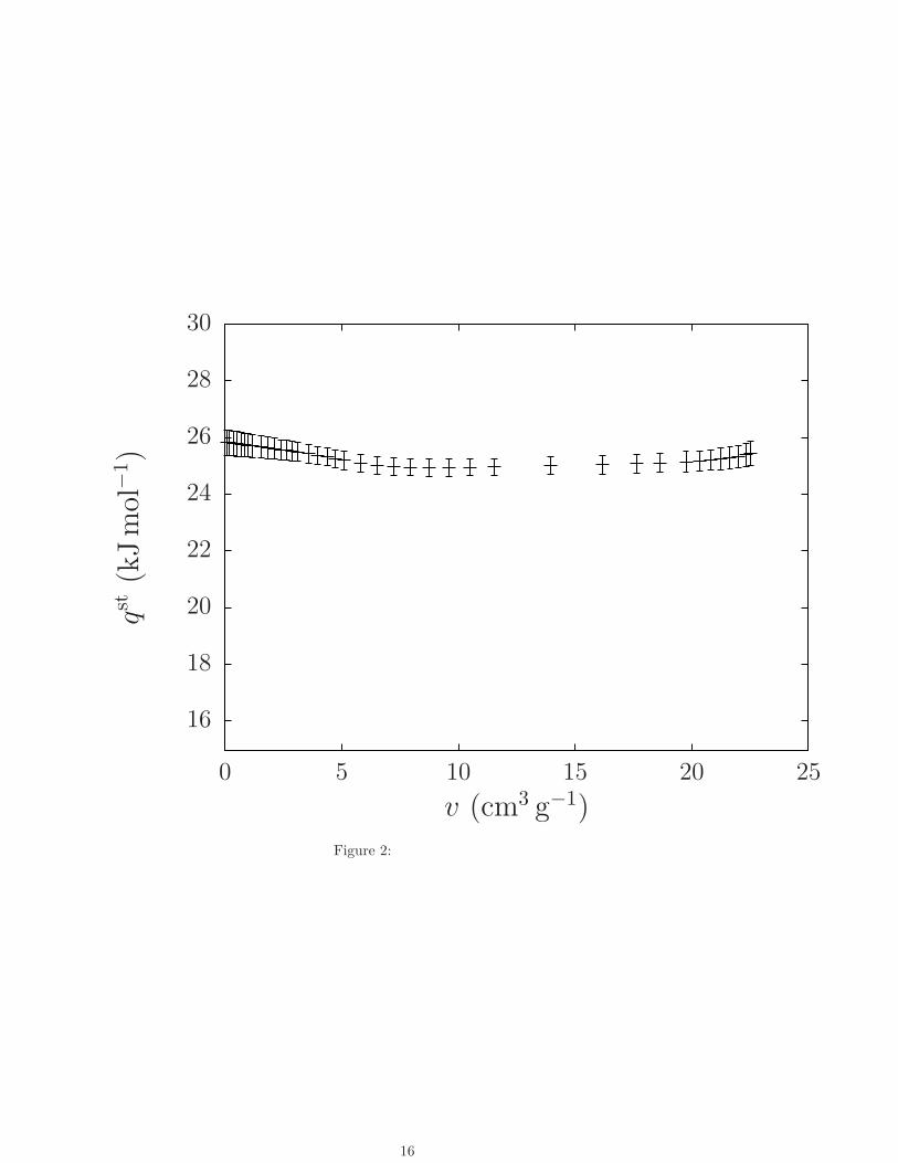
Fig. 2 shows the estimated isosteric heat of adsorption as a function of ad-sorbed volume and the corresponding marginal confidence intervals [5, 34] forthe SF6+W-A(673) system. This Fig. shows that qst is nearly constant around25.5 kJ/mol. Bandosz et al. [4] used a virial isotherm [9, 15] to correlate theirdata. They obtained plots of qst with some oscillations near zero saturationaround 25 kJ/mol; this result does not agree with that obtained here by meansof Eq. (23). These differences might be due to the method used by Bandosz etal. [4]. They fitted small subsets of 15 adsorption data by using the virial-typeisotherm and four parameters to fit each subset. Although this method is ap-propriate to fit the saturation data, the error bars reported by them correspondto standard deviations in the calculated isosteric heats of adsorption. If 95 %marginal confidence intervals are used, the error bars at low coverage would belarger and the oscillations in the isosteric heat might be within such error bars.

To illustrate the dependence of the isosteric heat of adsorption in terms oftemperature, plots of qst vs T at three different saturations are shown in Fig.3. As expected, the isosteric heat of adsorption does not significantly changewithin the experimental range of temperatures; this is typically observed in bothexperiments and molecular simulations. In the case in which it is necessary totake into account the dependency of isosteric heat of adsorption on temperature,the well known thermochemical formula [26] to calculate chemical equilibriumconstants could be used to estimate lnKj as a function of temperature in Eq.(4); an empirical model for the heat capacity would be necessary.

The fitting of the experimental isotherms of adsorption of 1,1,1,2,3,3,3-heptafluoropropane (HFC-227ea) on activated carbon is shown in Fig. 4. As

1For this system, the saturation is expressed as a volume at 101.325 kPa and 273.15 K

8

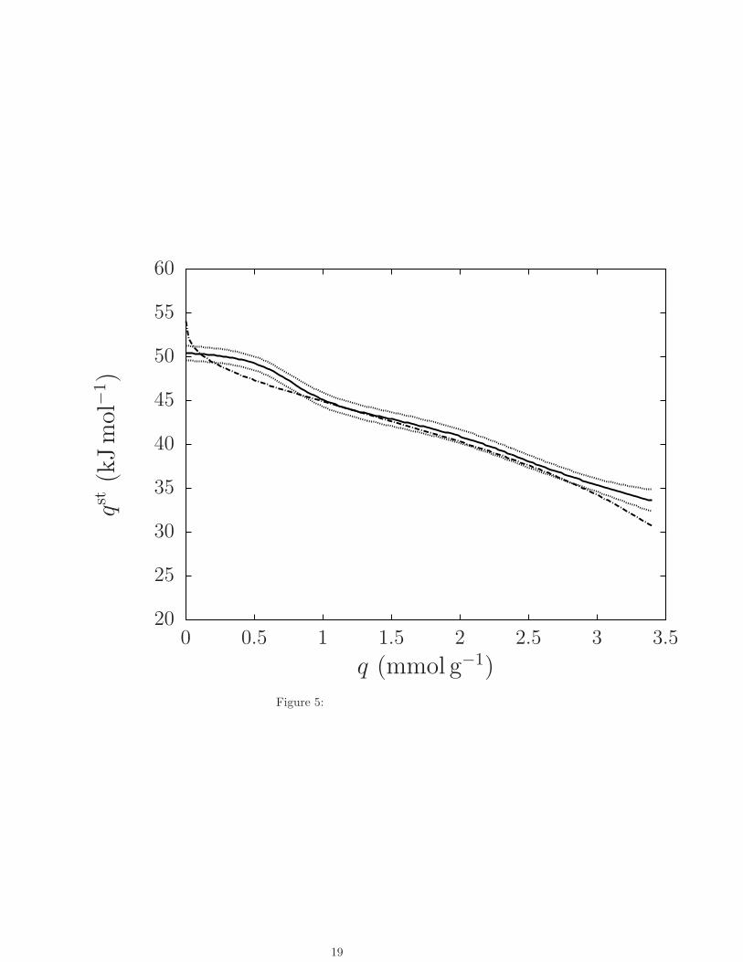
in the previous case, the fittings are very accurate; the correction term was notnecessary (l = 0). Due to the complex pore structure of activated carbon, it isdifficult to consider a subsystem as any specific region of the real adsorbent, forthis reason it is convenient to regard each cell as an effective subsystem. Theisosteric heat of adsorption calculated by using both Eq. (23) and the Tothequation are shown in Fig. 5. It can be noticed that both curves fairly agree.The differences are attributed to the fact that Yun et al. [42] only used twoisotherms to calculate the isosteric heat of adsorption. They employed the pa-rameters of each isotherm and the Clausius-Clapeyron equation to obtain theqst vs q plot. In contrast, here the complete set of experimental isotherms wasused. A problem with the method of Yun et al. [42] is that the isosteric heatof adsorption is influenced by uncertainties in the adsorption data, and hence,very reliable isotherms are necessary to determine qst if only two isotherms areto be employed.

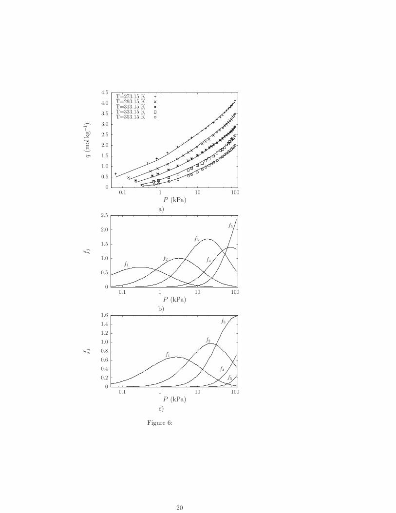
The adsorption isotherms of CO2 on zeocarbon [19] and the fractions ofmolecules distributed among cells at 273.15 K and 313.15 K are shown in Fig.6. The zeocarbon synthesized by Lee et al. [19] is a zeolite X/activated carbonmixture composed by 38.5 mass % zeolite X, 35 mass % activated carbon, 10mass % inert silica, and 16.5 mass % zeolite A and P. For this system, Eq.(18) accurately fits the experimental data (D = 3.8%), and the correction term(l = 1) in this case reduces the deviation by 2 % with respect to the l = 0 case.The deviation is less than that obtained by using the Toth equation; which isone of the most used equations to fit these kind of adsorption data. Since thezeocarbon is a zeolite/activated carbon composite, that the adsorbate phasemay be divided into identical weakly-interacting effective subsystems is again asuitable assumption for fitting and correlation purposes.

As it was mentioned in the previous section, at low pressures the leading termis f1 and each fj significantly contributes within a certain region of the isotherm.It can be noticed in Fig. 6a that the saturation (q) changes approximately0.5 mol kg−1 near 100 kPa. At the lowest experimental temperature for whichat high pressures the saturation is approximately qm, the leading term is fns+1,as shown in Fig. 6b. However, as temperature increases in the high experimentalpressure region, the isotherm turns into a combination of several fractions fj .For example, Fig. 6b shows that the isotherm at 313.15 K in the high pressureregion is a combination of f3, f4 and f5. When temperature is further increased,the term f5 does not contribute to the isotherm. If the correction term is notused and ns = 4, then the plot of f4 vs P is quite similar to that shown in Fig.6c for f5. Thus, this term does not significantly contribute to the isotherm at313.15 K. For this reason it was necessary to propose the correction terms shownin Eqs. (15) and (20). These Eqs. assure that high-order fractions depend onparameters that substantially contribute to estimate each isotherm within theexperimental temperature range. Because of the specific characteristics of eachadsorbate+adsorbent system, it is difficult to establish a priori whether thecorrection term is necessary; it must be tested whether this correction reducesthe fitting standard deviation.

The results of the fittings to the data reported in Ref. [41] are shown in

9

Table 2. In this case, Eq. (16) was used without corrections (l = 0). For theCO2+MSC and N2+MSC systems, Eq. (16) gives better results (in terms ofdeviation) than the simplified model (Eq. (18)). The deviation obtained withEq. (18) is around 3.5% (l = 0), whereas Eq. (6) gives deviations less than 3 %.Also, the deviation obtained using Eq. (16) is less than that obtained by usingthe Toth equation; this is also confirmed by F-tests. The confidence intervalsfor lnR◦

j are larger than those obtained for lnK◦ in Table 1. This could becaused by parameter correlation effects. To fit this set of isotherms, Watson etal. [41] used the Toth isotherm and also obtained large confidence intervals forthe K◦ parameter. For the CH4 system, the Toth isotherm gives better resultsthan Eqs. (6) and (18). This is due to an isotherm at 148 K that present anapparent saturation limit that is less than each of the apparent saturation limitsof the isotherms at temperatures greater than 148 K. If this isotherm at 148 Kis ignored, then the results obtained by using the 5-parameter Toth Eq. andEq. (16) are quite similar.

The advantage of the present models is the flexibility of setting the numberof adjustable parameters; this condition is essential to fit isotherms with com-plex shapes. Many of the widely used empirical isotherms to describe type Iisotherms like the Sips, Toth, and Dubinin-Ashtakov isotherms have fixed num-ber of parameters. Moreover, these Eqs. do not reduce to the correct Henry’slaw limit; except the Toth isotherm, but it overestimates the Henry’s constant[37]. In contrast, the GSTA model has the advantage that they present thecorrect Henry’s law limit and thus they can be used to estimate this constant.Despite its advantages, the model studied here cannot give site energy and poresize distribution. Although the model does not explicitly take into account theadsorbent heterogeneity, the number of parameters and the degree of the poly-nomial ξ, which are related to the subsystem size, might offer information aboutthe variety of adsorbent sites and molecule-molecule interaction.

4 Conclusions

It was found that the Eqs. (16) and (18) can be applied to fit experimental dataof adsorption of gases and vapours on microporous heterogeneous adsorbents.A simple correction that improve the fitting results was proposed. However,this correction may not be necessary in some cases, it must be tested. Addi-tionally, for systems in which the experimental temperature range is large, itis suggested that the dependence of ∆hj on temperature should be consideredand a model for both gas and adsorbate phase heat capacity could be required.The advantages of the GSTA model are the high accuracy that can be achievedto correlate saturation and thermodynamic data, the flexibility to set the num-ber of adjustable parameters and consider variations of lnKj with temperature,and the possibility of regarding the adsorptive as a real gas phase. However, themethod studied here does not explicitly consider the pore size and adsorptionsite energy distribution, but the size of a representative subsystem offers anidea of the adsorbent heterogeneity because the size of the subsystem depends

10

on this factor.

5 References

References

[1] G. L. Aranovich, J. S. Erickson, and M. D. Donohue. J. Chem. Phys., 120:5208–5216, 2004.

[2] K. G. Ayappa. J. Chem. Phys., 111:4736–4742, 1999.

[3] K. G. Ayappa, C. R. Kamala, and T. A. Abinandanan. J. Chem. Phys.,110:8714–8721, 1999.

[4] T. J. Bandosz, J. Jagie l lo, and J. A. Schwarz. J. Chem. Eng. Data, 41:880–884, 1996.

[5] D. M. Bates and D. G. Watts. Nonlinear Regression Analysis and its

Applications. Wiley, New York, 1988.

[6] K. Berlier and M. Frere. J. Chem. Eng. Data, 42:533–537, 1997.

[7] B. Boddenberg, G. U. Rakhmatkariev, and R. Greth. J. Phys. Chem. B,101:1634–1640, 1997.

[8] B. Boddenberg, G. U. Rakhmatkariev, S. Hufnagel, and Z. Salimov. Phys.Chem. Chem. Phys., 4:4172–4180, 2002.

[9] L. Czepirsky and J. Jagie l lo. Chem. Eng. Sci., 44:797–801, 1989.

[10] D. D. Duong. Adsorption Analysis: Equilibria and Kinetics. ImperialCollege Press, London, 1998.

[11] S. J. Gregg and K. S. W. Sing. Adsorption, Surface Area and Porosity.Academic Press, London, 1982.

[12] T. L. Hill. J. Phys. Chem., 57:324–329, 1953.

[13] T. L. Hill. Statistical Mechanics. McGraw–Hill, New York, 1956.

[14] T. L. Hill. An Introduction to Statistical Thermodynamics. Addison–Wesley, Reading, MA, 1960.

[15] J. Jagie l lo, T. J. Bandosz, K. Putyera, and J. A. Schwarz. J. Chem. Eng.

Data, 40:1288–1292, 1995.

[16] M. R. Kamat and D. Keffer. Mol. Phys., 100:2689–2701, 2002.

[17] D. G. Kinnlburgh. Environ. Sci. Technol., 20:895–904, 1986.

[18] I. Langmuir. J. Am. Chem. Soc., 40:1361–1403, 1918.

11

[19] J. Lee, J. Kim, J. Kim J. Suh, J. Lee, and C. Lee. J. Chem. Eng. Data,47:1237–1242, 2002.

[20] M. Llano-Restrepo. Adsorpt. Sci. Technol., 28:579–599, 2009.

[21] M. Llano-Restrepo. Fluid Phase Equilibr., 293:225–236, 2010.

[22] M. Llano-Restrepo and M. A. Mosquera. Fluid Phase Equilibr., 283:73–88,2009.

[23] J. Narkiewicz-Micha lek, P. Szabelski, W. Rudzinski, and A. S. T. Chiang.Langmuir, 15:6091–6102, 1999.

[24] P. Nikitas. J. Phys. Chem., 100:15247–15254, 1996.

[25] T. Nitta, M. Kuro-oka, and T. Katayama. J. Chem. Eng. Japan, 17:39–45,1984.

[26] I. Prigogine and R. Defay. Chemical Thermodynamics. Longmans Greenand Co, New York, 1954.

[27] A. J. Ramirez-Pastor, T. P. Eggarter, V. Pereyra, and J. L. Riccardo. Phys.Rev. B, 59:11027–11036, 1999.

[28] A. J. Ramirez-Pastor, V. D. Pereyra, and J. L. Ricardo. Langmuir, 15:5707–5712, 1999.

[29] J. L. Riccardo, F. Roma, and A. J. Ramirez-Pastor. Appl. Surf. Sci., 252:505–511, 2005.

[30] F. Roma, J. L. Ricardo, and A. J. Ramirez-Pastor. Langmuir, 21:2454–2459, 2005.

[31] D. M. Ruthven. Nat. Phys. Sci., 232:70–71, 1971.

[32] D. M. Ruthven and K. F. Loughlin. J. Chem. Soc. Farad. Trans. I, 68:696–708, 1972.

[33] D. M. Ruthven and F. Wong. Ind. Eng. Chem. Fund., 24:27–32, 1985.

[34] G. A. F. Seber and C. J. Wild. Nonlinear Regression. Wiley, New York,1989.

[35] R. Sips. J. Chem. Phys., 16:490–495, 1948.

[36] R. Sips. J. Chem. Phys., 18:1024–1026, 1950.

[37] J. M. Smith, H. C. Van Ness, and M. M. Abbott. Introduction to Chemical

Engineering Thermodynamics. McGraw-Hill, New York, 2005.

[38] H. Stach, U. Lohse, H. Thamm, and W. Schirmer. Zeolites, 6:74–90, 1986.

[39] W. A. Steele. J. Phys. Chem., 67:2016–2023, 1963.

12

[40] J. Toth. Acta Chim. Acad. Sci. Hung., 69:311–328, 1971.

[41] G. Watson, E. F. May, B. F. Graham, M. A. Trebble, R. D. Trengove, andK. I. Chan. J. Chem. Eng. Data, 54:2701–2707, 2009.

[42] J. Yun, D. Choi, and Y. Lee. J. Chem. Eng. Data, 45:136–139, 2000.

13

Figures:

Figure 1. Comparison between the experimental data of SF6 adsorption on W-A(673) [4] and Eq. (6); symbols: experiment, solid line: Eq. (18).Figure 2. Plot of isosteric heat of adsorption vs adsorbed volume, the systemtemperature is 283.0 K; error bars correspond to 95 % confidence intervals.Figure 3. Isosteric heat of adsorption for SF6+WA-(673) as a function of tem-perature at three different saturations.Figure 4. Comparison between the experimental data of HFC-227ea adsorptionon activated carbon [42] and Eq. (18); symbols: experiment, solid line: Eq.(18).Figure 5. Calculated isosteric heat of HFC-227ea adsorption on activated car-bon; dotted/dashed line: calculated by Yun et al. [42], solid line: Eq. (23),dotted lines: 95 % marginal confidence intervals for Eq. (23).Figure 6. a) Comparison between the experimental data of CO2 adsorption onzeocarbon [19] and Eq. (6); b) distribution of molecules among cells at 273.15K; c) same as b) for 313.15 K.

14

0

5

10

15

20

25

0 20 40 60 80 100

v(c

m3g−

1)

P (kPa)

T=266.5 KT=283.0 KT=297.5 K

Figure 1:

15

16

18

20

22

24

26

28

30

0 5 10 15 20 25

qst(k

Jm

ol−

1)

v (cm3 g−1)

Figure 2:

16

24.0

24.5

25.0

25.5

26.0

225 250 275 300 325 350

qst(k

Jm

ol−

1)

T (K)

v = 0.1 (cm3 g−1)v = 12.0 (cm3 g−1)v = 22.0 (cm3 g−1)

Figure 3:

17

0

0.5

1.0

1.5

2.0

2.5

3.0

3.5

0.01 0.1 1 10 100

q(m

mol

g−

1)

P (kPa)

T=283.15 KT=303.15 KT=333.15 KT=363.15 K

Figure 4:

18

20

25

30

35

40

45

50

55

60

0 0.5 1 1.5 2 2.5 3 3.5

qst(k

Jm

ol−

1)

q (mmol g−1)

Figure 5:

19

0

0.5

1.0

1.5

2.0

2.5

3.0

3.5

4.0

4.5

0.1 1 10 100

q(m

olkg−

1)

P (kPa)

T=273.15 KT=293.15 KT=313.15 KT=333.15 KT=353.15 K

a)

0

0.5

1.0

1.5

2.0

2.5

0.1 1 10 100

fj

P (kPa)

f1

f2

f3

f4

f5

b)

0

0.2

0.4

0.6

0.8

1.0

1.2

1.4

1.6

0.1 1 10 100

fj

P (kPa)

f1

f2

f3

f4

f5

c)

Figure 6:

20

Table 1: Estimated parameters for several systems using Eq. 18.a,b,c,d

qm (or v) lnK◦ −10−3 ×∆hj/R D Temperature PressureSystem mmol g−1 (or cm3 g−1) K % range (K) range (kPa)

SF6+W-A(673)[4] 23.89± 0.44 −13.67± 0.16 3.107± 0.055 2.97 266.5-297.5 0.1-100l = 1 6.112± 0.077

8.08± 0.5011.62 ± 0.32

C3H8+W-A[4] 34.6± 3.9 −14.65± 0.30 3.391± 0.096 3.2 267-298 0.1-100l = 1 7.472± 0.097

10.8± 0.2314.8± 0.6017.9± 0.48

HFC-227ea+AC[42] 3.87± 0.27 −16.67± 0.27 6.066± 0.098 2.36 283.15-363.15 0.01-100l = 0 11.39 ± 0.19

16.38 ± 0.3220.82 ± 0.4524.71 ± 0.68

HFP+AC[42] 3.87± 0.20 −15.66± 0.20 5.429± 0.075 2.53 283.15-363.15 0.01-100l = 0 10.15 ± 0.15

14.68 ± 0.2318.69 ± 0.3222.33 ± 0.45

CO2+ZC[19] 4.82± 0.39 −15.71± 0.29 5.03± 0.10 3.84 273.15-353.15 0.05-100l = 1 9.39± 0.20

13.45 ± 0.3117.00 ± 0.43

CO2+SG[6] 14.5± 1.0 −15.22± 0.10 3.068± 0.030 1.47 278-328 50-3400l = 4 5.759± 0.052

8.454± 0.09410.87 ± 0.12

a In all cases, P 0 is expressed in kPa.b Abbreviations: activated carbon (AC), 1,1,1,2,3,3,3-heptafluoropropane (HFC-227a),hexafluoropropene (HFP), zeocarbon (ZC), silica gel (SG).c The parameters ∆hj are tabulated in increasing order of j, e.g., for the SF6+W-A(673)system, ∆h1/R = −3.107× 103, ∆h2/R = −6.112× 103, and so on.d For SF6+W-A(673) and C3H8+W-A systems, the saturation is expressed in cm3 g−1 at

101.325 kPa and 273.15 K, and for the remaining systems it is expressed in mmol g−1.

Table 2: Estimated parameters for the adsorption data presented by Watson etal.[41] using Eq. 16 (l=0).a,b,c

qm lnR◦

j−10−3 ×∆hj/R D Temperature Pressure

System mmol · g−1 K % range (K) range (kPa)CH4+MSC 4.412± 0.067 −14.4± 1.5 2.81± 0.41 2.29 148-298 1-4000

−13.88 ± 0.48 1.92± 0.13CO2+MSC 5.87± 0.14 −13.7± 1.3 3.26± 0.40 1.41 223-323 25-5200

−14.00 ± 0.83 2.94± 0.25−16.07 ± 0.82 3.29± 0.22−19.46 ± 0.58 3.58± 0.17

N2+MSC 5.75± 0.12 −15.6± 1.1 2.71± 0.31 3.14 115-298 0.01-5000−14.03 ± 0.45 1.725± 0.099−18.3± 1.0 1.79± 0.15

a In all cases, P 0 is expressed in kPa.b Abbreviation: molecular sieving carbon (MSC).c As in 1, the parameters lnR◦

jand ∆hj are tabulated in increasing order of j, for example,

for the CH4+MSC system, lnR◦

1= −14.4, lnR2 = −13.88,

∆h1/R = −2.81× 103, ∆h2/R = −1.92× 103.

21