simula tion of p ar tiall y sa tura ted - fs.fed.us tion of p ar tiall y sa tura ted-flo w in the...

SIMULATION OF PARTIALLY SATURATED - SATURATED

FLOW IN THE CASPAR CREEK E-ROAD

GROUNDWATER SYSTEM

by

Jason C. Fisher

A Thesis

Presented to

The Faculty of Humboldt State University

In Partial Fulllment

of the Requirements for the Degree

Master of Science

In Environmental Systems: Environmental Resources Engineering

May 2000

SIMULATION OF PARTIALLY SATURATED - SATURATED

FLOW IN THE CASPAR CREEK E-ROAD

GROUNDWATER SYSTEM

by

Jason C. Fisher

Approved by the Master's Thesis Committee:

Dr. Robert Willis, Major Professor Date

Dr. Margaret Lang, Committee Member Date

Dr. Brad Finney, Committee Member Date

Jack Lewis, Committee Member Date

Roland Lamberson, Graduate Coordinator Date

Ronald A. Fritzsche, Date

Dean of Research and Graduate Studies

ABSTRACT

Over the past decade, the U.S. Forest Service has monitored the subsurface

hillslope ow of the E-road swale. The swale is located in the Caspar Creek wa-

tershed near Fort Bragg, California. In hydrologic year 1990 a logging road was

built across the middle section of the hillslope followed by a total clearcut of the

area during the following year. Development of the logging road has resulted in

a large build up of subsurface waters upslope of the road. The increase in pore

pressures behind the road is of major concern for slope stability and road failure.

A conceptual model is developed to describe the movement of water within the E-

road groundwater system. The two-dimensional SUTRA model is used to describe

both saturated and partially saturated ow within the system. SUTRA utilizes a

nite element and integrated nite dierence method to approximate the governing

equation for ow. The model appears to reproduce the uniquely dierent frequency

responses within the E-Road groundwater system. A comparison of simulated and

historical piezometric responses demonstrates the model's inability to reproduce

historical drainage rates. The low rates of simulated drainage are attributed to the

absence of pipe ow within the model. Finally, road consolidation is associated with

increased pore water pressures beneath the road bed.

iii

ACKNOWLEDGMENTS

I would like to express my thanks to the U.S. Forest Service Redwood Sciences

Laboratory for their encouragement and support of my work. A special thanks

goes to Liz Keppeler and her crew for maintaining the eld equipment during the

life of this study. I am grateful to Randi Field, co-worker and friend, for the many

discussions we shared on the topic of E-Road. I would also like to thank Dr. Robert

Willis, a compass in a sea of partial dierential equations.

iv

TABLE OF CONTENTS

LIST OF TABLES . . . . . . . . . . . . . . . . vii

LIST OF FIGURES . . . . . . . . . . . . . . . . viii

NOMENCLATURE . . . . . . . . . . . . . . . . xi

INTRODUCTION . . . . . . . . . . . . . . . . 1

HISTORY OF HILLSLOPE GROUNDWATER MODELS . . . 2

DESCRIPTION OF FIELD SITE AND INSTRUMENTATION . 7

Piping . . . . . . . . . . . . . . . . . . . 14

Pore Pressure . . . . . . . . . . . . . . . . 14

Rainfall . . . . . . . . . . . . . . . . . . 19

MODEL FORMULATION AND DEVELOPMENT . . . . . 22

DESCRIPTION OF MODEL SCENARIOS . . . . . . . . 28

Scenario 1: Homogeneous and Isotropic . . . . . . . . 28

Scenario 2: Nonhomogeneous with Active Boundary . . . 28

Scenario 3: Road Consolidation . . . . . . . . . . 31

MODEL RESULTS . . . . . . . . . . . . . . . . 32

Scenario 1: Sensitivity Analysis and Drainage Simulation . . 32

Scenario 2: Pre-Road Building . . . . . . . . . . . 41

Scenario 3: Post-Road Building and Historical Comparisons . 43

CONCLUSIONS . . . . . . . . . . . . . . . . . 52

REFERENCES . . . . . . . . . . . . . . . . . 53

APPENDIX A: Physical-Mathematical Basis of Numerical Model 57

Fluid Physical Properties . . . . . . . . . . . . 57

v

Properties of Fluid Within the Solid Matrix . . . . . . 58

Fluid Flow and Flow Properties . . . . . . . . . . 62

Partially Saturated Conditions . . . . . . . . . . . 66

Fluid Mass Balance . . . . . . . . . . . . . . 78

APPENDIX B: Numerical Methods . . . . . . . . . . 82

Basis Functions . . . . . . . . . . . . . . . . 82

Coordinate Transformations . . . . . . . . . . . 88

Gaussian Integration . . . . . . . . . . . . . . 90

Numerical Approximation of Fluid Mass Balance . . . . 94

Spatial Integration . . . . . . . . . . . . . . 95

Temporal Discretization . . . . . . . . . . . . . 102

APPENDIX C: Scenario 1 Sensitivity . . . . . . . . . . 104

APPENDIX D: Sample SUTRA.d55 Input File . . . . . . 106

vi

LIST OF TABLES

Table 1: Annual maximum pore pressure within the E-Road piezometers . 19

Table 2: Scenario 1 parameters for base case simulation . . . . . . 33

Table 3: Partially saturated parameters for seven soil types . . . . . 35

Table 4: Scenario 2 parameters . . . . . . . . . . . . . 42

vii

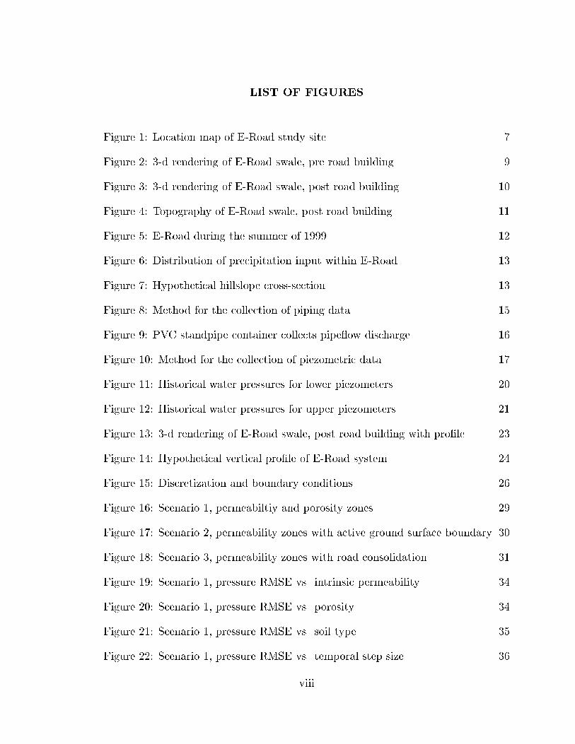
LIST OF FIGURES

Figure 1: Location map of E-Road study site . . . . . . . . . 7

Figure 2: 3-d rendering of E-Road swale, pre road building . . . . . 9

Figure 3: 3-d rendering of E-Road swale, post road building . . . . . 10

Figure 4: Topography of E-Road swale, post road building . . . . . 11

Figure 5: E-Road during the summer of 1999 . . . . . . . . . 12

Figure 6: Distribution of precipitation input within E-Road . . . . . 13

Figure 7: Hypothetical hillslope cross-section . . . . . . . . . 13

Figure 8: Method for the collection of piping data . . . . . . . . 15

Figure 9: PVC standpipe container collects pipe ow discharge . . . . 16

Figure 10: Method for the collection of piezometric data . . . . . . 17

Figure 11: Historical water pressures for lower piezometers . . . . . 20

Figure 12: Historical water pressures for upper piezometers . . . . . 21

Figure 13: 3-d rendering of E-Road swale, post road building with prole . 23

Figure 14: Hypothetical vertical prole of E-Road system . . . . . 24

Figure 15: Discretization and boundary conditions . . . . . . . . 26

Figure 16: Scenario 1, permeabiltiy and porosity zones . . . . . . 29

Figure 17: Scenario 2, permeability zones with active ground surface boundary 30

Figure 18: Scenario 3, permeability zones with road consolidation . . . 31

Figure 19: Scenario 1, pressure RMSE vs. intrinsic permeability . . . . 34

Figure 20: Scenario 1, pressure RMSE vs. porosity . . . . . . . 34

Figure 21: Scenario 1, pressure RMSE vs. soil type . . . . . . . 35

Figure 22: Scenario 1, pressure RMSE vs. temporal step size . . . . 36

viii

Figure 23: Scenario 1, computational time vs. temporal step size . . . 37

Figure 24: Scenario 1, pressure RMSE vs. number of elements . . . . 38

Figure 25: Scenario 1, compuational time vs. total number of elements . . 38

Figure 26: Scenario 1, parameter sensitivity . . . . . . . . . 39

Figure 27: Scenario 1, pressure contours, drainage of system over 27.8 hr . 40

Figure 28: Scenario 1, velocity vectors after 13.9 hr of simulation . . . 41

Figure 29: Scenario 2, pressure contours after 61 days of simulation . . . 43

Figure 30: Scenario 2, velocity vectors after 61 days of simulation . . . 43

Figure 31: Scenario 3, pressure contours after 61 days of simulation . . . 44

Figure 32: Scenario 3, velocity vectors after 61 days of simulation . . . 44

Figure 33: Historical and simulated (scenario 3) heads for piez. R1P2 . . 47






Figure 39: A comparison between scenario 2 and 3 for piez. R4P2 . . . 50

Figure A.1: Seepage through an inclined sand lter . . . . . . . 63

Figure A.2: Variations in x within a conceptual soil structure . . . . 68

Figure A.3: Unknown pore conguration . . . . . . . . . . 69

Figure A.4: Computed D based on 45 soils as a function of the power n . 73

Figure A.5: Water saturation versus pressure . . . . . . . . . 77

Figure A.6: Relative permeability versus pressure . . . . . . . . 77

ix

Figure A.7: Mass conservation for a control volume . . . . . . . 79

Figure B.1: A quadrilateral element . . . . . . . . . . . . 83

Figure B.2: Basis function dened for quadrilateral elements . . . . . 86

Figure B.3: Perspectives of basis function j(; ) at node j . . . . . 87

Figure B.4: Finite element in local coordinate system with Gauss points . 91

Figure B.5: Geometry of example cell i . . . . . . . . . . . 92

Figure B.6: Cells, elements, and nodes . . . . . . . . . . . 96

Figure B.7: Temporal denitions . . . . . . . . . . . . . 102

x

NOMENCLATURE

-Porous matrix compressibility

-Coecient of compressibility of water

-Porosity

-Horizontal distance in a local coordinate system

8 -The total spatial volume of the groundwater system

8e -Elemental volume

8total -Total volume of the porous medium composed of solid grains and void space

8void -Volume of void space in total volume

8water -Volume of water in total volume

-Specic weight of water

-The surface of the region to be simulated

-Dynamic viscosity of uid

r -Divergence operator

p -The average medium conductance

-Basis function within the local coordinate system

-Basis function within the global coordinate system

-Number between -1 and 1

-Fluid density

0

-Intergranular stress

-Vertical distance in a local coordinate system

xi

a -Scaling factor

A -Cross-sectional area

Ae -Eective area

Asat -Pore area at saturation

B -Thickness of the mesh within the y-coordinate direction

c -Shape factor

C -Proportionality constant

d -Mean grain diameter

D -The mean square deviation between krm and kr

g

-Magnitude of the gravitational acceleration vector

gp -Gauss point number

h -hydraulic head

hpiez -piezometric head

Hgp -Weighting coecients

i -Unit vectors in the x coordinate directions

I -Mass in ow rate

Ix -Mass in ow in the x direction

j -Unit vectors in the y coordinate directions

J -Jacobian Matrix

k -Intrinsic permeability

k -Unit vectors in the z coordinate directions

kr -Relative permeability

xii

krm -Relative permeabiltiy found through experiment

K -Hydraulic conductivity

l -Unitless

L -Length

L -Length unit

Lsurf -Length of the ground surface boundary

m -A factor used to account for the tortuosity of pores

M -Constant which incorporates properties of the uid and solid matrix

M -Mass unit

Mf -Total mass of uid contained in a total volume.

n -Accounts for eects of tortuosity and correlation factors

n -Normal unit vector

Nsurf -Total number of nodes on the ground surface boundary

NN -The total number of nodes within the nite element mesh

np -The total number of Gauss points

O -Mass out ow rate

Op -Governing equation representing the uid mass balance

Ox -Mass out ow in the x direction

p -Fluid pressure

pATM -Atmospheric pressure

pc -Capillary pressure

pcent -Entry pressure

xiii

p

i -Base case pressure head at node i

pi -Pressure head specied at node i

pBCi-Pressure value specied within the ground surface boundary node

ppiez -Pressure within the base of the piezometer

pproj

-An estimate of uid pressure at the end of the present time step

P -A point located at the centroid of a control volume

q -Mean seepage velocity of the uid

q -Specic discharge

Q -Rate of uid ow

Qp -Fluid mass source term

Qtip -Instantaneous tipping bucket records

r -Pore radius

re -Eective radius

Rp -A spatially varying residual value

RMSE -Root Mean Squared Error

s -Spatial Distance

Se -Eective saturation

Sop -Specic pressure storativity

Sw -Water saturation

Swres -A residual saturation below which saturation is not expected to fall

t -Time

T -Time unit

xiv

u -Connectivity of pore structure

v

-Average uid velocity

Wi -Weighting function in global coordinates

x -Horizontal spatial distance within the global coordinate system

y -Spatial depth within the global coordinate system

z -Vertical spatial distance within the global coordinate system

zelev -Elevation of the piezometers base

xv

INTRODUCTION

Over the past decade, the U.S. Forest Service has monitored the subsurface hill-

slope ow of the E-road swale. The swale is located in the Caspar Creek watershed

near Fort Bragg, California. Monitoring has consisted of piezometric measurements

recorded every 15 to 30 minutes from well sites located throughout the swale and

pipe ow measurements at 10 min intervals. In hydrologic year 1990 a logging road

was built across the middle section of the hillslope followed by a total clearcut of

the area during the following year.

Development of the logging road has resulted in a large build up of subsurface

waters behind the road. The road behaves much like a dam, and road and slope

stability are of major concern. Landslides commonly occur during rainstorms when

soil saturation reduces soil shear strength. Pore water pressure is the only slope sta-

bility variable that changes over a short time scale, and theory predicts that a slope

can become unstable as saturated thickness increases due to rainfall inltration.

Previous studies of subsurface hillslope ow indicate that very little is understood

about the subject. Further studies in this area will only help to improve existing

techniques in the design and maintenance of mountain roads.

This investigation employs a conceptual model to better understand the hy-

drologic mechanisms which govern the behavior of subsurface waters within a swale

road system. A comparison is made between model simulations and historical E-

Road pore pressures.

1

HISTORY OF HILLSLOPE GROUNDWATER MODELS

Field investigations of subsurface hillslope ow have shown that piezometric re-

sponse is sensitive to rainfall, soil porosity, topography, and vegetation. Swanston

(1967) showed that there is a close relationship between rainfall and pore-water

pressure development. As rainfall increases, pore-water pressure increases, rapidly

at rst, but at a decreasing rate as rainfall continues, reaching an upper limit de-

termined by the thickness of the soil prole. Additional studies of shallow-soiled

hillslopes during the wet seasons showed that there was little lag time between

rainfall and piezometric response (Swanston, 1967; Hanberg and Gokce, 1992). Fur-

thermore, Hanberg and Gokce (1992) showed that the rate of piezometric rise was

dependent on porosity and rainfall rate. Keppeler et al. (1994) observed increases

in pore-water pressure and soil moisture following logging.

Based on eld evidence, Whipkey (1965), Hewlett and Nutter (1970), and

Weyman (1970) suggested that the presence of inhomogeneities in the soil may be

a crucial factor in the generation of subsurface storm ow. These inhomogeneities

may either be permeability breaks associated with soil horizons that allow shallow

saturated conditions to build up or as Harr (1977), Mosley (1979), and Beven (1980)

suggest, inhomogeneities may be structural and biotic macropores in the soil that

allow for very fast ow rates. With a signicant portion of the total subsurface ow

taking place in the macropores, a higher hydraulic conductivity will be perceived

for the entire soil prole. In addition eld studies of subsurface storm ow have

shown that the direct application of Darcian ow to subsurface water in forested

watersheds may not be realistic (Whipkey, 1965; Mosley, 1979).

2

3

Both analytical and numerical models of saturated hillslope subsurface ow

have been developed using the nonlinear Boussinesq equation, also called the Dupuit

Forchheimer equation. The second approximation of the Boussinesq (1904) equa-

tion, was modied by Bear (1972) to incorporate a non-horizontal bottom.

Bear (1972), Sloan and Moore (1984), and Buchanan et al. (1990) have all de-

veloped analytical solutions to predict piezometric response for subsurface saturated

ow in a one-dimensional uniform slope. While these models describe oversimpli-

ed groundwater systems quite well, the analytical solutions are unable to describe

anything complex in nature (e.g. a system found in the environment). However,

attempts have been made to further develop an analytical model to handle complex

transient recharge in a sloping aquifer of nite width (Singh et al., 1991).

A numerical model developed by Hanberg and Gokce (1992), modeled the full,

one dimensional Dupuit-Forchheimer equation for a hillside with changing slope

angle and transient rainfall. The predicted response rose with the historical observed

response but receded more quickly. They hypothesized that seepage out of the

bedrock lengthened the observed recession.

Reddi et al. (1990) numerically modeled saturated subsurface ow in the arial

two-dimensional space with pressures averaged over the vertical depth of the aquifer.

In the overall downslope direction the Dupuit-Forchheimer approach was used. Flow

in the transverse direction was assumed horizontal and was not topographically

driven. Their predictions diered signicantly from eld observations in timing and

magnitude. The rst physically-based numerical model to describe both partially

saturated and saturated ow within a hillslope system was presented by Freeze

4

(1972a). Freeze developed a hillslope model to study base ow generation in upland

watersheds, and storm runo processes (Freeze,1972b). Earlier, Freeze (1971) had

developed a single governing equation that encompasses both partially saturated

and saturated ow. The successive over-relaxation technique, an iterative technique

that employs implicit nite dierence formulations, is used to solve the nonlinear

parabolic partial dierential governing equation. Later work by Freeze (1974) and

Beven (1989) indicated the practical and theoretical limitations associated with

modeling complex natural ow systems with simulation models. These include:

parameter averaging, data uncertainty, spatial variability of important parameters,

computer limitations, and discretization.

Dietrich et al. (1986) simulated two-dimensional steady-state ow in a hypo-

thetical homogeneous hillslope using TRUST (Narasimhan et al., 1978). The model

is a partially saturated - saturated hillslope model that utilizes an integral nite

dierence method, incorporating both inltration partitioning and overland ow.

They found that the pore pressure distribution was strongly dependent on both

boundary conditions and slope geometry. Application of the TRUST model is ad-

ditionally seen in the work of Wilson (1988) and Brown (1995). Wilson (1988) and

Brown (1995) represented hillslope systems in both two and three dimensions. The

two-dimensional systems represented the vertical cross-section from an upper to

lower portion of the hillslope. The three-dimensional systems combined a number

of vertical cross-sections to dene the entire hillslope system.

Wilson (1988) found the hydraulic response was controlled by groundwater cir-

culation patterns within the bedrock resulting from large-scale topographic controls

5

and small-scale heterogeneities in bedrock permeability. Brown discovered that a

mixed explicit-implicit solver worked best for his study since it produced acceptable

mass balance results and did not show signicant oscillations for a range of materi-

als. Model simulations using available eld data were compared to eld observations

of rainfall pore-pressure responses and were found to be in reasonable agreement.

The nite dierence approximation of subsurface hillslope ow is again seen

in the work of Blain (1989) and Jackson (1992a). The hillslope subsurface system

was characterized in the arial two-dimensional space. Blain utilizes an upstream-

weighted dierence approximation of the spatial partial derivatives and a Crank-

Nicholson approximation for the temporal pattern of soil moisture. Jackson simpli-

es the system by assuming streamlines parallel to the slope and the domination of

saturated, subsurface ow. Additionally, the model has the capability to deal with

convergent (or divergent) topography. They found that peak piezometric response

was largely dependent on rainfall rate and the storage coecient while the recession

curve was in uenced mainly by the hydraulic conductivity. The model was tested

against piezometric response measured in a hillslope hollow and showed promising

results.

The application of a nite element model to hillslope subsurface ow was rst

seen in the work of Calver (1988, 1989). Calver utilized a rainfall-runo model, the

Institute of Hydrology Distributed Model version 4 [IHDM4], developed by Beven

et al. (1987). The Galerkin method of weighted residuals is used by the model for

the two spatial dimensions while an implicit nite dierence scheme is applied to

the time dimension. Calver conducted both two and three-dimensional simulations

6

for hillslope catchments. The two-dimensional system consisted of vertical sections

while the three-dimensional system required combining the vertical slices. Calver

found that generally smaller elements were favored with a ratio of horizontal to

vertical element dimension equal to 10. A temporal discretization of 0.5 hours was

found to be the longest possible time step.

Flow and transport modeling within the hillslope subsurface environment was

investigated by McCord et al. (1991) and Jackson (1992b). Both groups of modelers

applied VAM2D (Huyakorn et al., 1989), a nite element model which simulates ow

and transport in two spatial dimensions. Simulation results were then compared

to eld site tracer studies. McCord's results indicated that both soil type and

anisotropy strongly aect unsaturated ow.

Brandes et al. (1998) conducted numerical modeling experiments to solve the

steady state Richards' equation over a two-dimensional cross-sectional hillslope do-

main using the nite element model FEMWATER (Yeh, 1987). The system was

characterized by (1) no- ow (Neumann) boundary conditions along the sides and

base of the hillslope, (2) a variable inltration-seepage boundary along the ground

surface, and (3) a single constant head (Dirichlet) node at the foot of the slope

representing a rst-order stream. Brandes et al. looked at the model's behavior

under steady-state precipitation with low initial antecedent soil conditions. Results

from FEMWATER indicate that a decreasing unsaturated zone will provide stabil-

ity within the numerics of the solution as the saturated zone increases. Furthermore,

the hillslope system at or near complete saturation will exhibit instability.

DESCRIPTION OF FIELD SITE AND INSTRUMENTATION

The E-Road swale, a moderately steep zero-order basin, is located within the

headwaters of the North Fork Caspar Creek ExperimentalWatershed, in the Jackson

Demonstration State Forest near Fort Bragg, California, USA (Figure 1) (UTM

zone 10 E:438426 N:4356896). The north-facing swale has a youthful topography

consisting of uplifted marine terraces that date to the late Tertiary and Quaternary

periods (Kilbourne, 1986). The swale occupies an area of 0.40 hectares.

Figure 1: California, U.S.A., and location map of E-Road study site in the Caspar Creek Watershed.

Caspar Creek Watershed

Hw

y. 1

123o45’00"

39o22’30"

kilometers

0.5 0 0.5 1 1.5 2

Watershed BoundaryStreams

California

N E-Road Site

Dirt RoadsPaved Roads

NFC408 Raingauge

Precipitation within the study area is characterized by low-intensity rainfall,

prolonged cloudy periods in winter, and relatively dry summers with cool coastal

7

8

fog. Between October and April 90% of the 1190 mm mean annual occurs. Average

monthly air temperatures between 1990 and 1995 in December were 6:7C, with an

average minimum of 4:7C. Average July temperatures was 15:6C, with an average

maximum of 22:3C (Ziemer, 1996).

The soil within the swale is the Vandamme series, a clayey, vermiculitic,

isomesic typic tropudult, derived from sedimentary rocks, primarily Franciscan

greywacke sandstone. Textures of the surface soil and subsoil are loam and clay

loam respectively, with 35 to 45% clay in the subsoil (Keppeler, et al., 1994). The

permeability within the soil is considered moderately slow (Hu et al., 1985).

Vegetation within the swale is dominated by Douglas-r (Pseudotsuga menziesii

[Mirb.] Franco), coast redwood (Sequoia sempervirens [D.Don] Endl.), grand r

(Abies grandis [Dougl. ex D.Don] Lindl.), western hemlock (Tsuga heterophylla

[Raf.] Sarg.), tanoak (Lithocarpus densi orus [Hook. and Arn.] Rohn) and Pacic

madrone (Arbutus menziesii Pursh.).

The E-Road groundwater study began in hydrologic year 1990 and involved

the monitoring of pipe ow and pore pressures within the swale. Instrumentation

for piping and pore pressures was installed in the fall of 1989. During the winter of

1990, pre-disturbance monitoring took place until a seasonal road was constructed

across the swale in the summer of 1990. Tree removal required for road construction

was implemented using skyline cable yarding. In late-summer 1991, the timber in

the remainder of the swale was harvested using tractor yarding above the road

and long-lining below. In late November 1991, broadcast burning took place. Due

to the north-facing aspect of the swale, fuel consumption was incomplete. Three-

9

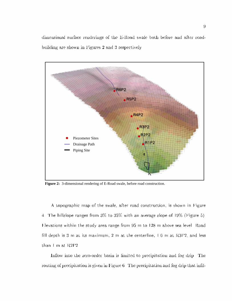
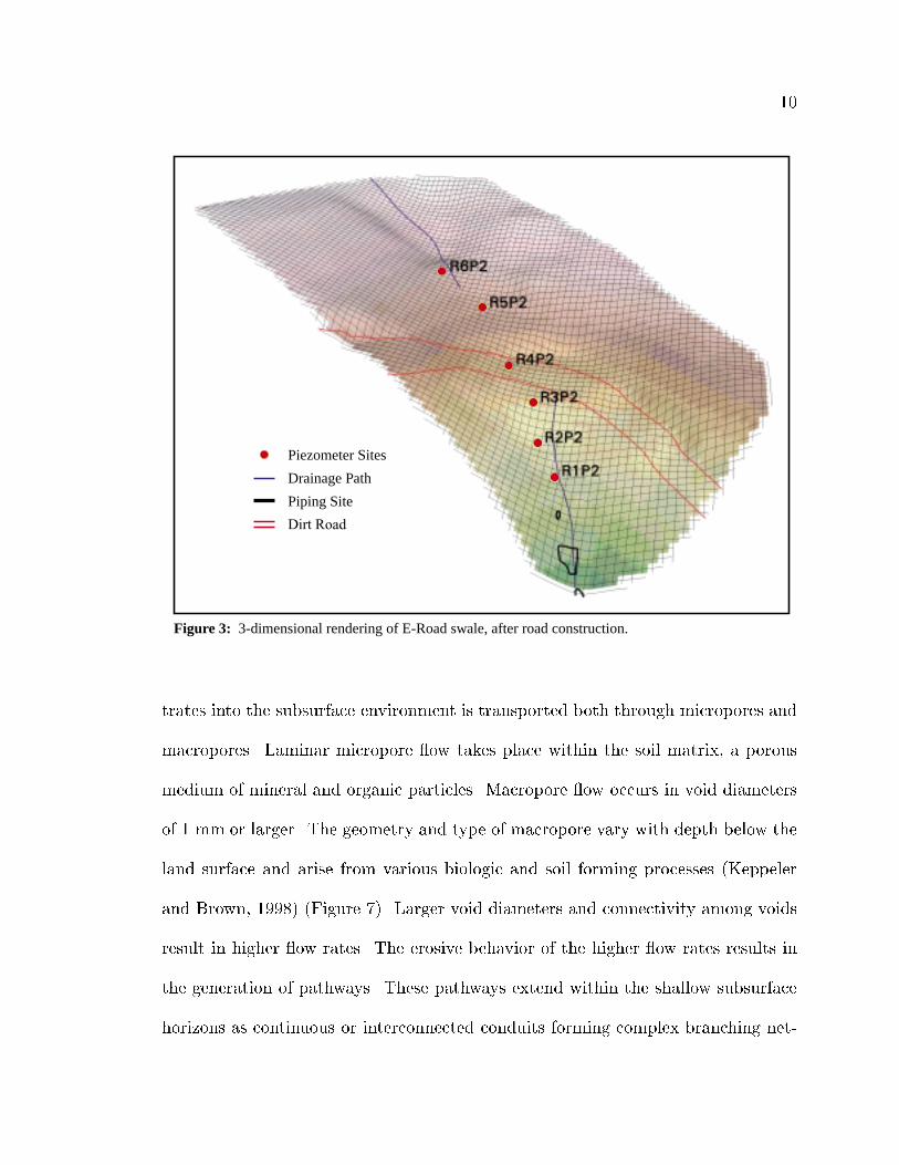
dimensional surface renderings of the E-Road swale both before and after road-

building are shown in Figures 2 and 3 respectively.

Figure 2: 3-dimensional rendering of E-Road swale, before road construction.

Piezometer Sites

Drainage Path

Piping Site

A topographic map of the swale, after road construction, is shown in Figure

4. The hillslope ranges from 3% to 35% with an average slope of 19% (Figure 5).

Elevations within the study area range from 95 m to 128 m above sea level. Road

ll depth is 3 m at its maximum, 2 m at the centerline, 1.6 m at R3P2, and less

than 1 m at R2P2.

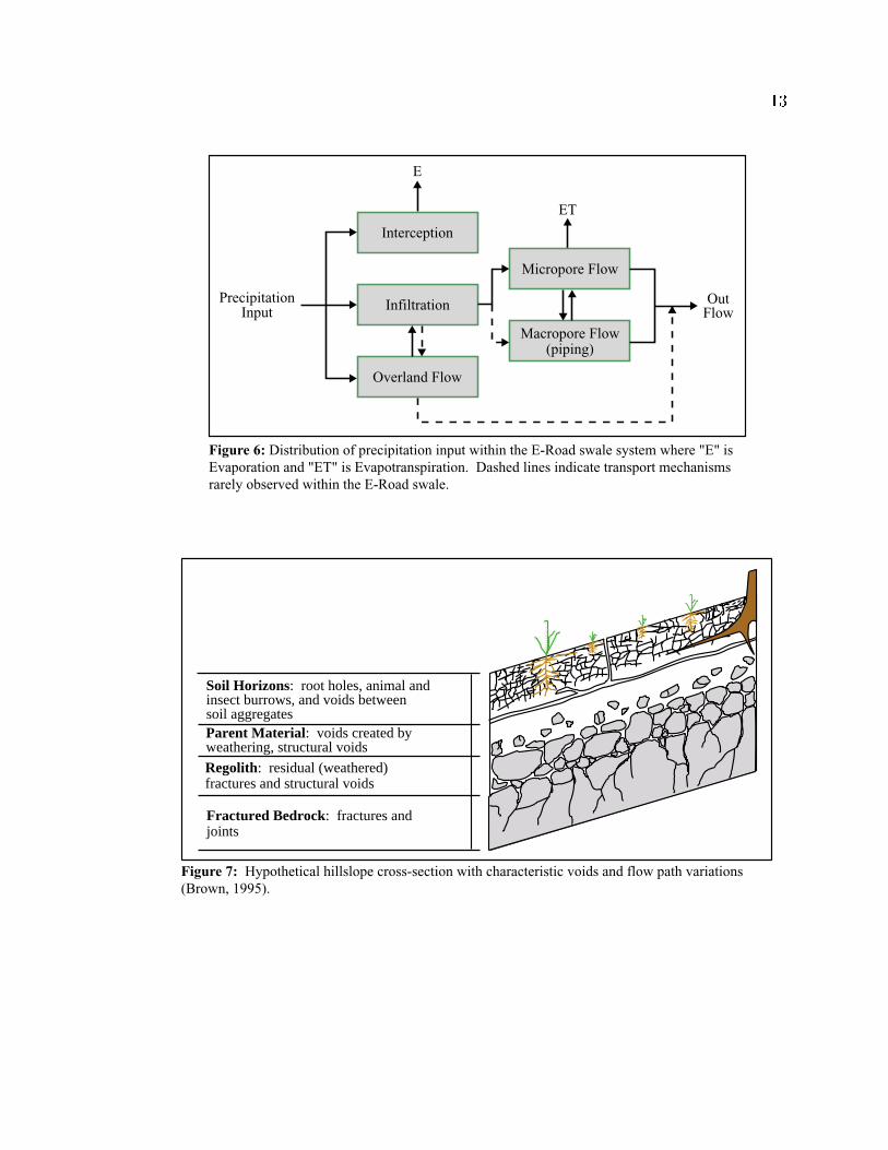
In ow into the zero-order basin is limited to precipitation and fog drip. The

routing of precipitation is given in Figure 6. The precipitation and fog drip that inl-

10

Figure 3: 3-dimensional rendering of E-Road swale, after road construction.

Piezometer Sites

Drainage Path

Piping Site

Dirt Road

trates into the subsurface environment is transported both through micropores and

macropores. Laminar micropore ow takes place within the soil matrix, a porous

medium of mineral and organic particles. Macropore ow occurs in void diameters

of 1 mm or larger. The geometry and type of macropore vary with depth below the

land surface and arise from various biologic and soil forming processes (Keppeler

and Brown, 1998) (Figure 7). Larger void diameters and connectivity among voids

result in higher ow rates. The erosive behavior of the higher ow rates results in

the generation of pathways. These pathways extend within the shallow subsurface

horizons as continuous or interconnected conduits forming complex branching net-

11

Contour Interval: 2m

Scale: 1:3330 10

0 1 2 3 cm

m

E_Road Piping

Survey Station

Step Ladder

Piezometer

Piping Hole

Ridge

Waterbar

Culvert

Culvert Drainage

Road Cut

Edge of Road Right-of-Way

Area of Road Fill

Rocked Surface

Plastic

W.B.

culvert

Bench Mark

96

98

100

102

104

108110

112

106

114

116

118

120

122

124

126

128

98

100102

104

106108

110112

114

116118120

122

124

126

128

96

R4P2

R1P2

R2P2

R5P2

R6P2

R3P2

CU

LVE

RT

WB

WB

WB

Figure 4: Topography of E-Road swale, post road building.

N

12

R4P2

Figure 5: E-Road during the summer of 1999.

works (Albright, 1992). Pipe ow is that ow which takes place through conduits 2

cm or greater in diameter.

For the duration of the E-Road study, data collected have included pipe ow,

pore pressure, and rainfall data. Collection methods and instrumentation for each

type of data are discussed below.

13

Infiltration

E

Interception

Overland Flow

PrecipitationInput

Figure 6: Distribution of precipitation input within the E-Road swale system where "E" is Evaporation and "ET" is Evapotranspiration. Dashed lines indicate transport mechanisms rarely observed within the E-Road swale.

ET

Macropore Flow(piping)

Micropore Flow

OutFlow

Soil Horizons: root holes, animal andinsect burrows, and voids between soil aggregatesParent Material: voids created by weathering, structural voids

Regolith: residual (weathered) fractures and structural voids

Fractured Bedrock: fractures and joints

Figure 7: Hypothetical hillslope cross-section with characteristic voids and flow path variations(Brown, 1995).

14

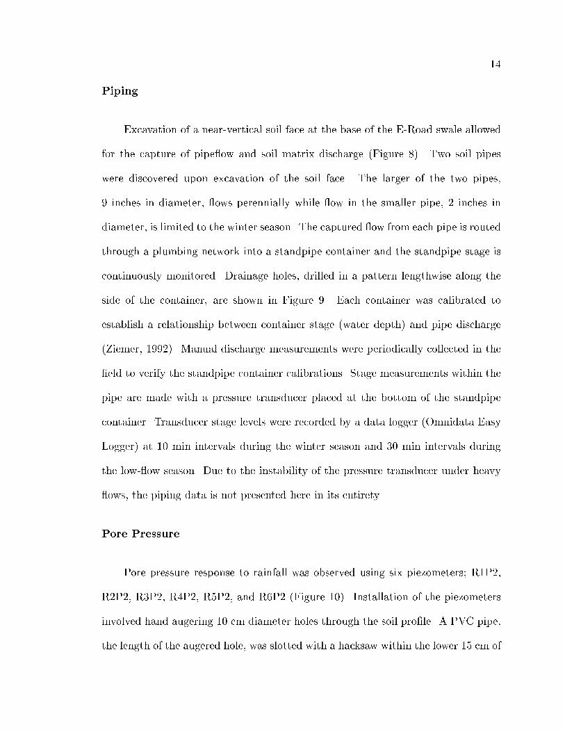
Piping

Excavation of a near-vertical soil face at the base of the E-Road swale allowed

for the capture of pipe ow and soil matrix discharge (Figure 8). Two soil pipes

were discovered upon excavation of the soil face. The larger of the two pipes,

9 inches in diameter, ows perennially while ow in the smaller pipe, 2 inches in

diameter, is limited to the winter season. The captured ow from each pipe is routed

through a plumbing network into a standpipe container and the standpipe stage is

continuously monitored. Drainage holes, drilled in a pattern lengthwise along the

side of the container, are shown in Figure 9. Each container was calibrated to

establish a relationship between container stage (water depth) and pipe discharge

(Ziemer, 1992). Manual discharge measurements were periodically collected in the

eld to verify the standpipe container calibrations. Stage measurements within the

pipe are made with a pressure transducer placed at the bottom of the standpipe

container. Transducer stage levels were recorded by a data logger (Omnidata Easy

Logger) at 10 min intervals during the winter season and 30 min intervals during

the low- ow season. Due to the instability of the pressure transducer under heavy

ows, the piping data is not presented here in its entirety.

Pore Pressure

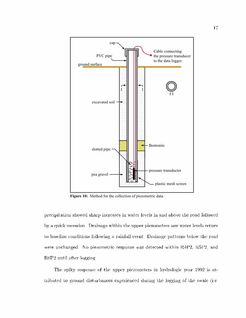
Pore pressure response to rainfall was observed using six piezometers; R1P2,

R2P2, R3P2, R4P2, R5P2, and R6P2 (Figure 10). Installation of the piezometers

involved hand augering 10 cm diameter holes through the soil prole. A PVC pipe,

the length of the augered hole, was slotted with a hacksaw within the lower 15 cm of

15

Step ladder

Regolith and Fractured Bedrock

Parent Material

Soil Horizons

PVC pipe

PVC pipegrouted tohillslope.

Figure 8: Method for the collection of piping data.

soil pipes

Cable connectingthe pressure

to the datalogger.

transducer

Standpipe Container

the pipe. After wrapping the slotted portion of the pipe with a plastic mesh screen,

the entire pipe was lowered into the augered hole. The pipe was then backlled

with approximately 25 cm of pea gravel, 15-20 cm of bentonite, and excavated soil.

Depth of the augered holes was limited by the physical limit of the hand augering

device. At some sites, rock fragments in the lower saprolite prevented the auger

from reaching bedrock (Keppeler and Brown, 1998). The water level within the

pipe was measured with a pressure transducer and electronically recorded by data

logger. Fluid pressures are recorded at 15 min intervals during the winter and 30 min

intervals during the summer months. Manual stage measurements were periodically

taken with a hand-held water level detector to validate pressure transducer data.

Figures 11 and 12 show water levels for each of the piezometers over time. Maximum

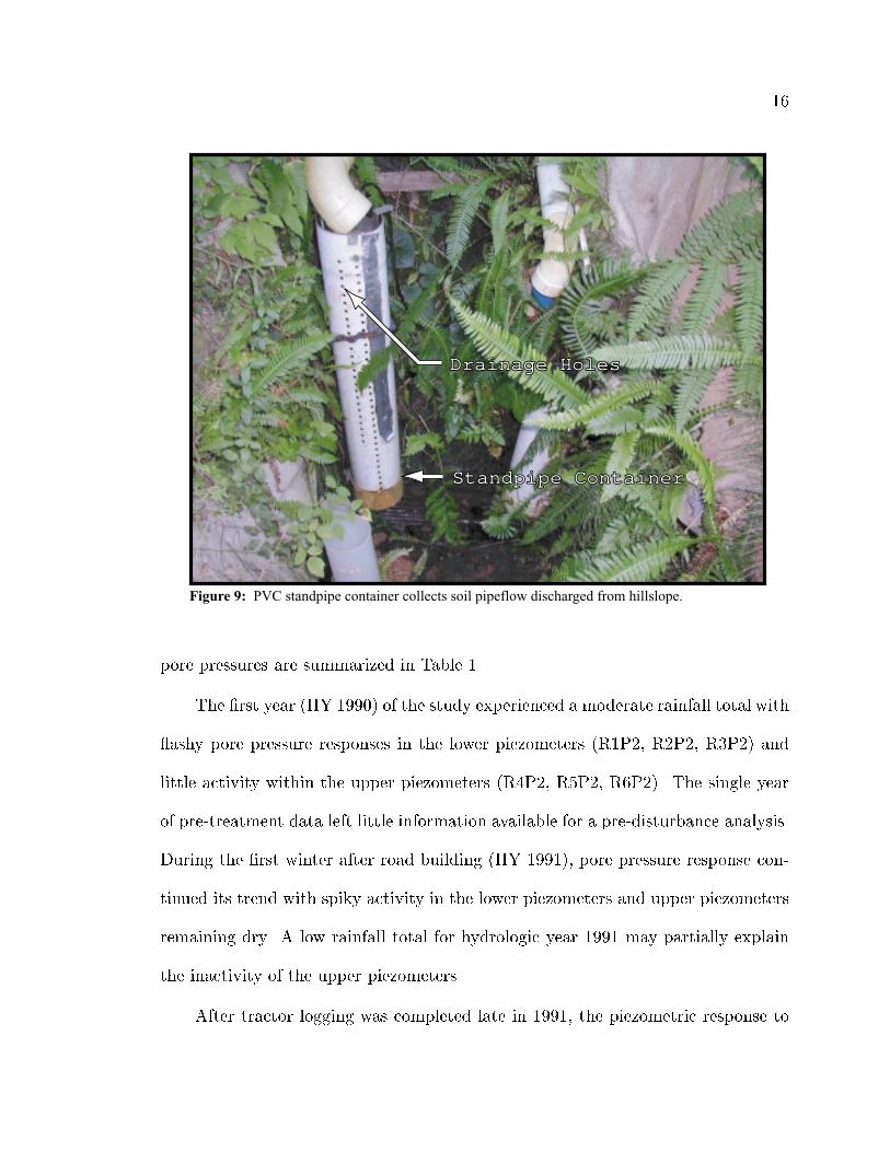
16

Standpipe Container

Drainage Holes

Figure 9: PVC standpipe container collects soil pipeflow discharged from hillslope.

pore pressures are summarized in Table 1.

The rst year (HY 1990) of the study experienced a moderate rainfall total with

ashy pore pressure responses in the lower piezometers (R1P2, R2P2, R3P2) and

little activity within the upper piezometers (R4P2, R5P2, R6P2). The single year

of pre-treatment data left little information available for a pre-disturbance analysis.

During the rst winter after road building (HY 1991), pore pressure response con-

tinued its trend with spiky activity in the lower piezometers and upper piezometers

remaining dry. A low rainfall total for hydrologic year 1991 may partially explain

the inactivity of the upper piezometers.

After tractor logging was completed late in 1991, the piezometric response to

17

Figure 10: Method for the collection of piezometric data.

PVC pipe

ground surface

cap

Cable connectingthe pressure transducerto the data logger.

slotted pipe

pea gravel

excavated soil

Bentonite

pressure transducter

I II-I

plastic mesh screen

precipitation showed sharp increases in water levels in and above the road followed

by a quick recession. Drainage within the upper piezometers saw water levels return

to baseline conditions following a rainfall event. Drainage patterns below the road

were unchanged. No piezometric response was detected within R4P2, R5P2, and

R6P2 until after logging.

The spiky response of the upper piezometers in hydrologic year 1992 is at-

tributed to ground disturbances experienced during the logging of the swale (i.e.

18

the collapse of soil pipes beneath the roadbed). Damage to the established piping

network directly aects the swales ability to drain. Following the clearcut, rain-

fall events act to re-establish the damaged pipe network. Pore pressures, up-slope

from a collapsed pipe, increase until pressures are sucient enough to reshape the

piping network. New soil pipes are formed within the patchwork of collapsed pipes

allowing for an increase in drainage rates.

In hydrologic year 1993, a high rainfall year, the uid pressure response to dis-

crete rainfall events changed drastically within the upper piezometer holes. Their

ashy response was now superimposed on an annual rise-fall cycle. The compound-

ing of pore pressures throughout the winter months indicates a groundwater build-

up behind the road which is assumed to result from the consolidation of road bed

materials and a consequent decrease in drainage rates beneath the road surface.

The magnitude of groundwater buildup is both a function of the annual precipi-

tation total and the antecedent precipitation index (API) entering into the winter

months.

Low rainfall for hydrologic year 1994 saw a decrease in groundwater buildup in

and above the road; however, the compounding response was still evident through-

out the year. From hydrologic year 1995 to 1998 the E-Road swale experienced

much higher annual rainfall totals. The response of the system to increased pre-

cipitation was a clear buildup of groundwater behind the road during the winter

months followed by the gradual drainage of the system throughout the summer

months. In hydrologic year 1998 the swale received 88 inches; the highest annual

rainfall total. The response of pore pressures beneath the road to elevated precipi-

19

tation levels resulted in a record water level of 6.42 m for piezometer R4P2 (Table

1). The increase in uid pressure beneath the road, arguably the weakest portion of

the hillslope (road-ll), raises the potential for hillslope failure. Water levels within

R4P2 have never returned to pre-disturbance levels.

Table 1: Annual maximum pore pressures within the E-Road piezometers. NR indicates that nopositive pressure head was observed during that year.

RainfallHydro Year R1P2 R2P2 R3P2 R4P2 R5P2 R6P2 Total (in)

199019911992199319941995199619971998

44.7328.7536.5662.7734.4163.5551.8851.4287.98

Max. Pore Pressure (m)Hole Depth (m)

0.370.570.650.610.420.520.460.450.480.651.37

1.311.711.912.092.121.921.881.801.842.122.59

2.113.396.054.244.294.504.495.594.536.056.35

0.770.636.034.613.895.254.694.076.426.427.66

NRNR2.974.773.974.724.844.934.904.935.69

NRNR6.454.186.567.496.766.047.417.497.83

Water level with respect to piezometer hole depth (m).

Base Elevation (m) 101.01 101.53 101.57 102.31 108.79 109.74

Rainfall

Rainfall is monitored with the NFC408 tipping bucket rain gauge (UTM zone

10 E:439243 N:4357978) located 1.335 km north-east of the E-Road swale. Data

collection is instantaneous with each tip recording 0.01 inches of rainfall. An Onset

data logger is used to electronically record tip times. Figures 11 and 12 show daily

rainfall totals for hydrologic years 1990 through 1998 with annual rainfall totals

summarized in Table 1.

100

102

104

106

100

102

104

106

Aug Sep Oct Nov Dec Jan Feb Mar Apr May Jun Jul

0

1

2

3

4

5

Aug Sep Oct Nov Dec Jan Feb Mar Apr May Jun Jul Aug Sep Oct Nov Dec Jan Feb Mar Apr May Jun Jul

HY 1993 HY 1994 HY 1995

Wat

er E

leva

tion

(m)

Prec

ip. (

in)


0

1

2

3

4

5


HY 1996 HY 1997 HY 1998

Wat

er E

leva

tion

(m)

Prec

ip. (

in)

r3p2


0

1

2

3

4

5


HY 1990 HY 1991 HY 1992

Piez. Elec. Obs.

r1p2r2p2

CLEAR-CUTLOGGING

ROADCONSTRUCTION

Wat

er E

leva

tion

(m)

Prec

ip. (

in)

Figure 11: Historical piezometric responses for R1P2, R2P2, and R3P2.

20

100

102

104

106

105

110

115


0

1

2

3

4

5


HY 1993 HY 1994 HY 1995

Wat

er E

leva

tion

(m)

Prec

ip. (

in)

105

110

115


0

1

2

3

4

5


HY 1996 HY 1997 HY 1998

Wat

er E

leva

tion

(m)

Prec

ip. (

in)

r6p2

105

110

115


0

1

2

3

4

5


HY 1990 HY 1991 HY 1992

Piez. Elec. Obs.

r4p2r5p2

CLEAR-CUTLOGGING

ROADCONSTRUCTION

Wat

er E

leva

tion

(m)

Prec

ip. (

in)

Figure 12: Historical piezometric responses for R4P2, R5P2, and R6P2.

21

MODEL FORMULATION AND DEVELOPMENT

Development of a two-dimensional model required a simplication of the swale

system. In Figure 13, a prole line was established through the center of the swale

connecting each of the piezometer sites. Both upper and lower segments of the

prole follow the swale's drainage path. A vertical cross-section established along

the prole line allowed for a two dimensional (2-d) hypothetical prole view of

the hillslope (Figure 14), where elevation is measured in the vertical coordinate

direction. Representation of the swale system in two dimensions neglects the eects

of convergent ow.

Fluid ow within the 2-d model is limited to the horizontal (x-axis) and vertical

(z-axis) directions with pore pressures averaged over the thickness (y-axis) of the

system. The error associated with a 2-d representation of a 3-d system is not easily

quantied in a complex environmental system such as the E-Road swale. However,

future investigations may address the error associated with neglecting convergent

ow by comparing 2-d and 3-d numerical representations of the E-Road system.

Evapotransporation, interception, and pipe ow are additional hydrologic mech-

anisms unaccounted for by the model. A reduction in rainfall is assumed to partially

account for evapotranspiration and interception. Pipe ow, however, is not as eas-

ily accounted for by the model. The governing equation, describing groundwater

ow within the system, is built upon the assumption of laminar ow. Flow within

soil pipes is turbulent and little is known about the spatial distribution of soil

pipes within the E-Road swale. Impacts associated with neglecting pipe ow are

not clearly understood. The importance of pipe ow is, however, a major hydrologic

22

23

Figure 13: 3-dimensional rendering of E-Road swale, after road-building, with profile connecting piezometer sites.

Piezometer Sites

Profile

mechanism within the swale system. Studies conducted for similar swale systems

within the Caspar Creek watershed attribute 99% of the total swale discharge to

pipe ow (Ziemer, 1992). The inability of inltrating waters to enter a piping system

is expected to translate into slower drainage rates within the swale. The purpose of

applying the numerical model is not to exactly represent the E-Road historical be-

havior, but rather to aid in understanding the mechanisms which govern subsurface

ow within a swale-road system.

A shortage of information within the subsurface environment required making

certain assumptions about the geometry and depth of subsurface material layers.

24

Horizontal Spatial Distance (m)

Ele

vatio

n A

bove

Sea

Lev

el (

m)

0 10 20 30 40 50 60 70 8095

100

105

110

115

120

125

130

Figure 14: Hypothetical vertical profile of E-Road system.

Mountain Ridge

Road Bed

Piping Site

R4P2

R1P2

R2P2

R3P2

R5P2

R6P2


Parent Material

Piezometers

Soil Horizons

Solid Bedrock

Phreatic Surface

Consolidated Regolith and Fractured Bedrock

Consolidated Parent Material

Placement of the regolith layer was aided with depth measurements for each of the

piezometers. It was assumed that the physical limitations associated with the hand

augering device put piezometer hole depths at the interface between parent and

regolith materials. Segmentation of the subsurface into zones of diering material

type (i.e. soil horizons, parent material, and regolith-fractured bedrock) allowed for

the allocation of subsurface parameters (e.g. permeability and porosity). In addi-

tion, materials are assumed to be consolidated beneath the road surface, because

of logging operations, vehicle trac, and road ll mass.

25

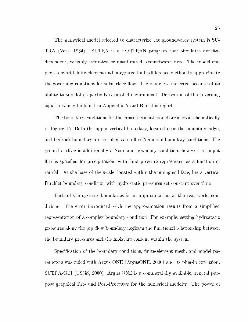
The numerical model selected to characterize the groundwater system is SU-

TRA (Voss, 1984). SUTRA is a FORTRAN program that simulates density-

dependent, variably saturated or unsaturated, groundwater ow. The model em-

ploys a hybrid nite-element and integrated nite-dierence method to approximate

the governing equations for subsurface ow. The model was selected because of its

ability to simulate a partially saturated environment. Derivation of the governing

equations may be found in Appendix A and B of this report.

The boundary conditions for the cross-sectional model are shown schematically

in Figure 15. Both the upper vertical boundary, located near the mountain ridge,

and bedrock boundary are specied as no- ux Neumann boundary conditions. The

ground surface is additionally a Neumann boundary condition, however, an input

ux is specied for precipitation, with uid pressure represented as a function of

rainfall. At the base of the swale, located within the piping soil face, lies a vertical

Dirchlet boundary condition with hydrostatic pressures set constant over time.

Each of the systems boundaries is an approximation of the real world con-

ditions. The error introduced with the approximation results from a simplied

representation of a complex boundary condition. For example, setting hydrostatic

pressures along the pipe ow boundary neglects the functional relationship between

the boundary pressures and the moisture content within the system.

Specication of the boundary conditions, nite-element mesh, and model pa-

rameters was aided with Argus ONE (ArgusONE, 2000) and its plug-in extension,

SUTRA-GUI (USGS, 2000). Argus ONE is a commercially available, general pur-

pose graphical Pre- and Post-Processor for the numerical modeler. The power of

26


Ele

vatio

n A

bove

Sea

Lev

el (

m)

0 10 20 30 40 50 60 70 8095

100

105

110

115

120

125

130

Figure 15: Discretization and boundary conditions.

Ground Surface

Bedrock

Mountain Ridge

Piping Site

Neumann B.C. (No-Flux)

Neumann B.C. (No-Flux)

Time Dependent Precipitation

Neumann B.C. (Rainfall-Flux)

Dirchlet B.C. (Hydrostatic)

Finite Element Mesh

Argus ONE is in its ability to generate robust nite-element meshes within com-

plex topographic boundaries. SUTRA-GUI, a public domain Graphical User Inter-

face (GUI) developed by the USGS for SUTRA, uses Argus ONE to automatically

prepare SUTRA input les and to provide immediate visualization of simulation

results.

A note is made of the computational tools utilized for the E-Road modeling

investigation. Simulations as well as pre- and post-processing were performed on a

PC, running Windows NT version 4.0 (service pack 6), with the following specs: one

27

ABIT BP6 Dual Socket 370 Celeron 440BX AGP 3xDIMMs ATX motherboard, two

Boxed Intel 366MHz Celeron PPGA Processors with 128KB L2 cache (each proces-

sor was over clocked to 500MHz), and one 16Mx64 3.3V SDRAM 168-pin DIMM

PC100 (128 MByte). Model simulations were run using the Microsoft Developer

Studio 97 (Visual Fortran Professional Edition 5.0A.)

DESCRIPTION OF MODEL SCENARIOS

A working model to describe the E-Road system was developed in three, in-

creasingly complex scenarios. Each phase, represented as a simulation scenario,

builds upon the complexity of the previous phase.

Scenario 1: Homogeneous and Isotropic

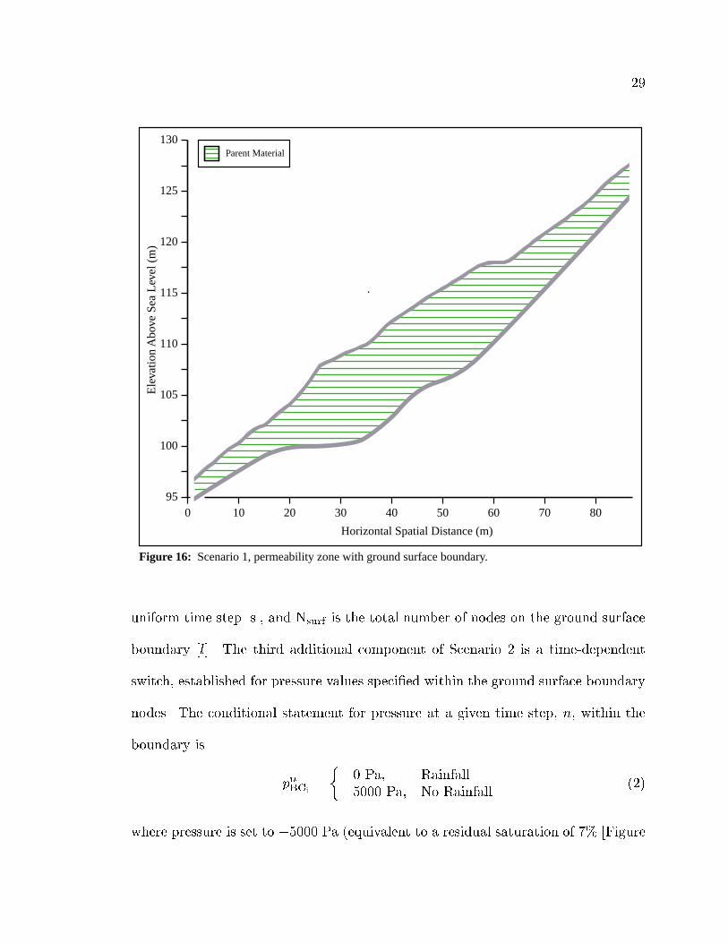
The rst scenario, shown in Figure 16, consists of a homogeneous and isotropic

E-Road groundwater system. The ground surface boundary is specied as a no- ux

Neumann boundary condition. Furthermore, without a rainfall ux, Scenario 1 is

restricted to drainage simulations. Initial pressures within the system at t = 0

re ect a totally saturated system. This scenario is used to investigate the model's

sensitivity to changes in parameters.

Scenario 2: Nonhomogeneous with Active Ground Surface Boundary

The second scenario, shown in Figure 17, is a nonhomogeneous system that

builds upon Scenario 1 with three additional components. First, intrinsic perme-

ability zones are established for the soil horizons, parent material, and regolith and

fractured bedrock. Secondly, a rainfall ux, Qp, is added across the ground surface

boundary. Converting instantaneous tipping bucket records, Qtip, from inches to

meters per second required

Qp =(Qtip)(0:0254

m

in)(Lsurf)(dy)

(t)(Nsurf)(1)

where Lsurf is the length of the ground surface boundary [m], dy is the width

of the system within the y-coordinate direction (set constant at 1 m), t is the

28

29


Ele

vatio

n A

bove

Sea

Lev

el (

m)

0 10 20 30 40 50 60 70 8095

100

105

110

115

120

125

130Parent Material

Figure 16: Scenario 1, permeability zone with ground surface boundary.

uniform time step [s], and Nsurf is the total number of nodes on the ground surface

boundary [l]. The third additional component of Scenario 2 is a time-dependent

switch, established for pressure values specied within the ground surface boundary

nodes. The conditional statement for pressure at a given time step, n, within the

boundary is

pnBCi

=

0 Pa; Rainfall

5000 Pa; No Rainfall(2)

where pressure is set to 5000 Pa (equivalent to a residual saturation of 7% [Figure

30

A.5]) for time periods of no rainfall, and atmospheric (gauge) pressure for periods

of rain. At atmospheric pressure, a spatial node is considered totally saturated,

Sw = 100%. Initial pressures within the system at t = 0 re ect a partially drained

system.


Ele

vatio

n A

bove

Sea

Lev

el (

m)

0 10 20 30 40 50 60 70 8095

100

105

110

115

120

125

130

Parent Material


Figure 17: Scenario 2, permeability zones with active ground surface boundary.

Soil Horizons

31

Scenario 3: Road Consolidation

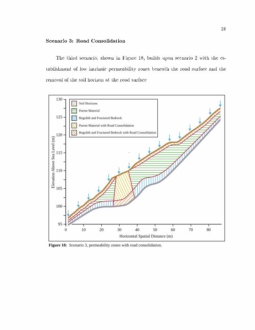
The third scenario, shown in Figure 18, builds upon scenario 2 with the es-

tablishment of low intrinsic permeability zones beneath the road surface and the

removal of the soil horizon at the road surface.


Ele

vatio

n A

bove

Sea

Lev

el (

m)

0 10 20 30 40 50 60 70 8095

100

105

110

115

120

125

130

Parent Material

Parent Material with Road Consolidation


Regolith and Fractured Bedrock with Road Consolidation

Figure 18: Scenario 3, permeability zones with road consolidation.

Soil Horizons

32

MODEL RESULTS

Simulation results are presented for each of the groundwater scenarios.

Scenario 1: Sensitivity Analysis and Drainage Simulation

The dierences between the simulation results from scenario 1 were quantied

using a root mean squared error (RMSE) criteria. The equation for the pressure

RMSE is

RMSE =

sPNN

i=1

(p

i pi)2

NN

(3)

where p

iis the base case pressure head at a specic spatial node i, pi is the pressure

head for a given run of the model, and NN is the total number of spatial nodes. The

RMSE quanties the dierence in pressure head conditions between two simulation

results for a given time period. Each of the two simulations share identical nite

element meshes, however, system parameters and boundaries dier between the

simulations.

The rst simulation is run with a set of parameters known as the `base case.'

Base case parameter values for scenario 1 are listed in Table 2. The second sim-

ulation utilizes parameter values identical to the base case with the exception of

a single parameter change. Incrementing a single parameter value over a range of

magnitudes generates a number of simulation results. These simulation results are

compared to the base case results using the RMSE.

A RMSE analysis is performed for the parameters: (1) intrinsic permeability,

(2) porosity, (3) soil type, (4) temporal step size, and (5) the total number of

elements within the system. A detailed description of the RMSE results is given in

33

Appendix C of this report. In Figures 19-22 and 24, the base case appears as the

point for which RMSE = 0.

Table 2: Scenario 1 parameters for base case simulation.

PARAMETER NOTATION VALUE UNITS

Volumetric Porosity POR, ε 0.1 UnitlessIntrinsic Permeability PMAX/MIN, k 1.0Ε−11 m2

Duration of time step DELT, ∆t 10 sec

Fractional upstream weight 0UP UnitlessPressure boundary-condition 0.01GNUP Unitless

Maximum allowed simulation time TMAX 100000 secFluid compressibility COMPFL, β 2.718E-6 (m sec2) / kgDensity of fluid RHOW0, ρ 1000 kg / m3

Solid matrix compressibility COMPMA, α 1.27E-6 (m sec2) / kgDensity of solid grain RHOS 1025 kg / m3

Component of gravity vector in the +X direction GRAVX 0 m / sec2

Component of gravity vector in the +Z direction GRAVY -9.81 m / sec2

Sandy clay loam: a 0.58 m-1Number of elements in systems 2696NE Unitless

Fluid Viscosity VISC0, µ 0.001 kg / (m sec)

n 1.59 UnitlessSsat 0.54 Unitless

Swres 0.09 Unitless

Scaling FactorShape ParameterWater saturation at saturationResidual saturation

The sensitivity of the model to intrinsic permeability, a measure of the ease of

uid movement through saturated interconnected void spaces, is shown in Figure

19. The range in intrinsic permeabilities is k = 1013m2 to k = 1010m2. Changes

to intrinsic permeabilities in the range (1013m2 < k < 1011m2) signicantly

impact the models solution while changes in the range (1011m2 < k < 1010m2)

have little to no impact.

The sensitivity of the model to porosity is shown in Figure 20. Recall, the

porosity is the volume of voids in the soil matrix per total volume. The range

in porosity is = 1% to = 30%. RMSE increases approximately linearly with

departures of porosity from the base case value.

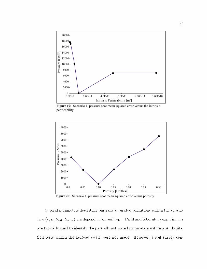
34

Figure 19: Scenario 1, pressure root mean squared error versus the intrinsicpermeability.

0

2000

4000

6000

8000

10000

12000

14000

16000

18000

20000

0.0E+0 2.0E-11 4.0E-11 6.0E-11 8.00E-11 1.00E-10

Pres

sure

RM

SE

Intrinsic Permeability [m2]

Figure 20: Scenario 1, pressure root mean squared error versus porosity.

0

1000

2000

3000

4000

5000

6000

7000

8000

9000

0.0 0.05 0.10 0.15 0.20 0.25 0.30

Pres

sure

RM

SE

Porosity [Unitless]

Several parameters describing partially saturated conditions within the subsur-

face (a, n, Ssat, Swres) are dependent on soil type. Field and laboratory experiments

are typically used to identify the partially saturated parameters within a study site.

Soil tests within the E-Road swale were not made. However, a soil survey con-

35

ducted for the watershed identied the soil type as `clay loam.' Table 3 gives the

range of dierent soil types utilized for the sensitivity analysis of partially saturated

parameters. A soil type of `sandy clay loam' is used in the base case simulation of

scenario 1.

Table 3: Partially saturated parameters for seven soil types.

SOIL TYPESSandy loamSilt LoamLoamSandy clay loamSilty clay loamClay loamBeit Netofa Clay

a n Ssat Swres2.77

10.9217.810.581.361.25

0.152

2.891.181.161.591.242.381.17

0.440.500.500.540.560.56

0.446

0.000.000.00

0.00

0.00

0.09

0.07

RMSE values calculated for each of the seven soil types are shown in Figure 21.

Similar simulation results are observed for silt loam, loam, and sandy clay loam.

Figure 21: Scenario 1, pressure root mean squared error versus soil type.

Pres

sure

RM

SE

0

500

1000

1500

2000

2500

3000

3500

4000

4500

SandyLoam

SiltLoam

Loam Sandy Clay Loam

Silty Clay Loam

Clay Loam

Beit Netofa Clay

Figure 22 shows RMSE values calculated for a range of temporal step sizes, t.

Theory suggests that a decrease in t increases the numerical stability of the model.

36

The tradeo associated with a smaller step size is an increase in computational time

(Figure 23). For temporal step sizes less than 40 sec, the model is very sensitive

to small changes in t. Decreasing the temporal step size results in a reduction in

the moisture levels within the systems partially saturated conditions. For larger t

values an upper limit is established at 200 sec. Simulations made with t > 200

sec produced irregular drainage patterns within the swale. The irregular drainage

patterns, evident in the model's inappropriate storage of water within the upper

portion of the swale, is attributed to a breakdown in the numerics.

Figure 22: Scenario 1, pressure root mean squared error versus temporal step size.

0

500

1000

1500

2000

2500

3000

3500

0 100 200 300 400 500

Temporal Step Size [sec]

Pres

sure

RM

SE

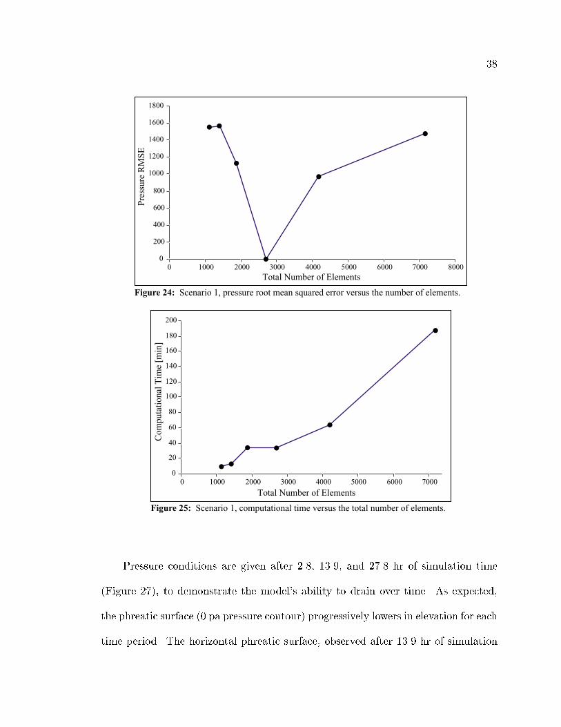
The sensitivity of the model to spatial discretization is established in Figure 24.

Figure 24 shows the pressure RMSE as a function of the total number of elements

within the system. Previous modeling investigations of a partially saturated system

indicate the susceptibility of the model to numerical breakdown given an insucient

number of elements (Fisher, 1999). The numerical instability was characterized by a

37

Figure 23: Scenario 1, computational time versus temporal step size.

Temporal Step Size [sec]

Com

puta

tiona

l Tim

e [m

in]

0

10

20

30

40

50

60

0 50 100 150 200

nonuniform capillary fringe along the phreatic surface. For scenario 1, the numerical

breakdown occurred for systems containing less than 1404 elements.

Greater numerical stability is achieved with an increase in the number of nite

elements within the system. In addition, a ner mesh density requires additional

computational time. Figure 25 gives the computational time as a function of the

total number of elements.

A maximum pressure RMSE is identied for each of the parameters previously

examined within the RMSE analysis. The magnitude of the maximum RMSE is

sensitive to the choice of base case and the range over which the parameter was

tested. A comparison of the maximum RMSE values is shown in Figure 26. Sen-

sitivity of the model is greatest for changes in intrinsic permeability. A moderate

sensitivity is observed for both the porosity and total number of elements. The

lowest sensitivity is associated with the soil type and temporal step size.

38

Figure 24: Scenario 1, pressure root mean squared error versus the number of elements.

Total Number of Elements

Pres

sure

RM

SE

0

200

400

600

800

1000

1200

1400

1600

1800

0 1000 2000 3000 4000 5000 6000 7000 8000

Figure 25: Scenario 1, computational time versus the total number of elements.


Com

puta

tiona

l Tim

e [m

in]

0

20

40

60

80

100

120

140

160

180

200

0 1000 2000 3000 4000 5000 6000 7000

Pressure conditions are given after 2.8, 13.9, and 27.8 hr of simulation time

(Figure 27), to demonstrate the model's ability to drain over time. As expected,

the phreatic surface (0 pa pressure contour) progressively lowers in elevation for each

time period. The horizontal phreatic surface, observed after 13.9 hr of simulation

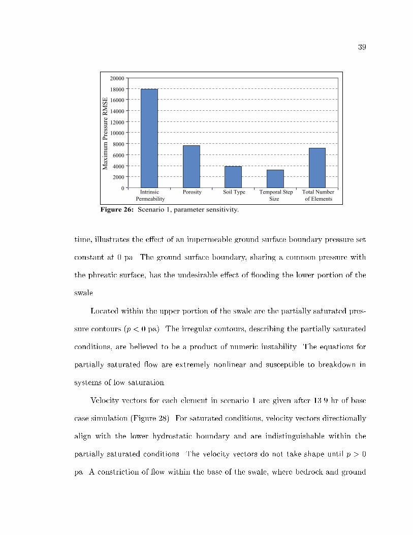
39

Figure 26: Scenario 1, parameter sensitivity.

Max

imum

Pre

ssur

e R

MSE

0

2000

4000

6000

8000

10000

12000

14000

16000

18000

20000

IntrinsicPermeability

Porosity Soil Type Temporal Step Size


time, illustrates the eect of an impermeable ground surface boundary pressure set

constant at 0 pa. The ground surface boundary, sharing a common pressure with

the phreatic surface, has the undesirable eect of ooding the lower portion of the

swale.

Located within the upper portion of the swale are the partially saturated pres-

sure contours (p < 0 pa). The irregular contours, describing the partially saturated

conditions, are believed to be a product of numeric instability. The equations for

partially saturated ow are extremely nonlinear and susceptible to breakdown in

systems of low saturation.

Velocity vectors for each element in scenario 1 are given after 13.9 hr of base

case simulation (Figure 28). For saturated conditions, velocity vectors directionally

align with the lower hydrostatic boundary and are indistinguishable within the

partially saturated conditions. The velocity vectors do not take shape until p > 0

pa. A constriction of ow within the base of the swale, where bedrock and ground

40

Figure 27: Scenario 1 pressure contours (pa), drainage of system over a time period of 2.8, 13.9, and 27.8 hours.

10 20 30 40 50 60 70 80

100

110

120E

leva

tion

Abo

ve S

ea L

evel

(m

) Elapsed Simulation Time: 2.8 hours

10 20 30 40 50 60 70 80

100

110

120

Ele

vatio

n A

bove

Sea

Lev

el (

m) Elapsed Simulation Time: 13.9 hours

10 20 30 40 50 60 70 80

100

110

120


Ele

vatio

n A

bove

Sea

Lev

el (

m) Elapsed Simulation Time: 27.8 hours

-10000 -5000

0 5000 10000 15000 20000 25000 30000 35000 40000 45000 50000 55000 60000 65000

surface boundaries merge, produces increased velocity magnitudes. Velocity vectors

exit the system through the lower hydrostatic boundary. The total mass ux across

41

10 20 30 40 50 60 70 80

100

110

120


Figure 28: Scenario 1, velocity vectors after 13.9 hours of simulation.

Ele

vatio

n A

bove

Sea

Lev

el (

m)

the lower hydrostatic boundary is 0.062 kg=m.

Scenario 2: Pre-Road Building

Scenario 2 parameters are summarized in Table 4. An increase in t was

required to complete a simulation run in a reasonable amount of time. At t =

200 sec, the 61-day simulation took approximately 14 hours to complete. Intrinsic

permeabilities within the system are given for each material type. A high intrinsic

permeability is specied in the soil horizons, a moderate intrinsic permeability in the

parent material, and a low intrinsic permeability within the regolith and fractured

bedrock. The time dependent rainfall ux, specied across the ground surface

boundary, is a function of historical rainfall records (November 10th 1996 to January

10th 1997).

Figure 29 depicts the pressure contours after 61 days of simulation. The shape

of the phreatic surface reveals the impact of intrinsic permeability layering within

the system. The placement of a higher intrinsic permeability zone over a lower

42

Table 4: Scenario 2 parameters (see Table 2 for undefined parameters).

PARAMETER NOTATION VALUE UNITS

Permeability: k 1.0Ε−11 m2

Duration of time step DELT, ∆t 200 secMaximum allowed simulation time TMAX 5270400 sec

Clay loam: a 1.25 m-1Number of elements in systems 3949NE Unitless

n 2.38 UnitlessSsat 0.56 Unitless

Swres 0.446 Unitless

Scaling FactorShape ParameterWater saturation at saturationResidual saturation

Soil HorizonsParent MaterialRegolith and Fractured Bedrock

6.0E-137.0E-14

m2

m2

intrinsic permeability zone produces a lag in the groundwater movement within the

regolith and fractured bedrock. The lag is most evident within the upper portion of

the swale where drainage rates are highest. The dierence in drainage rates between

the two material types is shown in Figure 30. Velocities within the parent material

are much greater than velocities within the regolith and fractured bedrock.

Flow within the soil horizons is dominated by gravity, with capillary forces

masked by the material's high intrinsic permeability. The only observable horizontal

ow within the soil horizons is found within the base of the swale. A constriction of

ow within the base forces the water table upward into the soil horizons. Unable to

enter back into the parent material, water is quickly transported out of the system

through the soil horizons. Velocity vectors, pointing outward across the ground

surface boundary, are responsible for ground seepage.

Simulations were made with reduced historic rainfall to test the sensitivity of

the model to changes in rainfall magnitude. Unexpectedly, there was no change

in the model solution for a 99% reduction in historical rainfall. The magnitude of

the mass ux across the ground surface boundary is negligible within the modeled

43

10 20 30 40 50 60 70 80

100

110

120


Figure 30: Scenario 2, velocity vectors after 61 days of simulation.

Ele

vatio

n A

bove

Sea

Lev

el (

m)

10 20 30 40 50 60 70 80

100

110

120


Figure 29: Scenario 2, pressure contours (pa) after 61 days of simulation.

Ele

vatio

n A

bove

Sea

Lev

el (

m)

-10000 -5000

0 5000 10000 15000 20000 25000 30000 35000 40000 45000 50000 55000 60000 65000

system. The pressure response to precipitation events is instead governed by the

model's pressure switch within the ground surface boundary.

Scenario 3: Post-Road Building and Historical Comparisons

Scenario 3 parameters are identical to scenario 2 parameters with the addition

of two low intrinsic permeability zones beneath the road surface. The intrinsic per-

meabilities of the two additional zones are k = 3 1012m2 within the consolidated

44

parent material and k = 6 1014m2 within the consolidated regolith and fractured

bedrock. Pressure contours and velocity vectors after a 61 day simulation period

are shown in Figures 31 and 32, respectively. The eect of road consolidation is an

increase in pore pressure beneath the road bed. Groundwater, impeded by the low

intrinsic permeability zone, mounds behind the consolidated material, reaching an

upper limit at the ground surface boundary.

10 20 30 40 50 60 70 80

100

110

120


Figure 32: Scenario 3, velocity vectors after 61 days of simulation.

Ele

vatio

n A

bove

Sea

Lev

el (

m)

10 20 30 40 50 60 70 80

100

110

120


Figure 31: Scenario 3, pressure contours (pa) after 61 days of simulation.

Ele

vatio

n A

bove

Sea

Lev

el (

m)

-10000 -5000

0 5000 10000 15000 20000 25000 30000 35000 40000 45000 50000 55000 60000 65000

45

For each of the swale's piezometers, a comparison is made between the water

year 1997 historical and simulated hydraulic heads (Figures 33-38). The conversion

from capillary pressure, p, to hydraulic head, h, is

hpiez =ppiez

+ zelev (4)

where hpiez is the piezometric head, ppiez is the pore water pressure within the base

of the piezometer, is the specic weight of water, and zelev is the elevation of

the piezometer's base. For the month of November 1996, the simulated pressure

response of the upper piezometers is strongly aected by the model's initial pressure

conditions. By December 1996 the in uence of the initial conditions is less apparent.

As seen in Figures 37 and 38, historical drainage rates are much greater than

simulated drainage rates. The dierence in drainage rates is attributed to the

model's inability to simulate pipe ow within the system. To compensate for pipe-

ow, intrinsic permeabilities were increased throughout the swale. The system's re-

sponse to higher intrinsic permeabilities is an increase in drainage within the upper

piezometers and a decrease in drainage within the lower piezometers. The decrease

in drainage emphasizes the control of the hydrostatic boundary on drainage rates

within the lower portion of the swale. Hydrostatic pressures, which are assumed con-

stant over time, place a limit on drainage across the swale's lower vertical boundary.

Groundwater, unable to exit the system at drainage rates associated with increased

intrinsic permeability, builds behind the hydrostatic boundary, ooding the lower

portion of the swale. The ooding is compounded by the excessive drainage rates

within the upper portion of the swale.

46

The model's overprediction of hydraulic heads within piezometer R4P2 (Figure

36) is not easily understood. Any number of hydrologic ow mechanisms, either

misrepresented or neglected within the system, may attribute to the approximately

4 m dierence between historical and simulated water pressures. Possible problem

areas include: (1) neglecting convergent ow within the 2-d system, (2) the incor-

rect placement of the bedrock boundary, (3) the inability of the model to simulate

pipe ow, and (4) an oversimplication of ground consolidation with depth. These

issues should be addressed in future groundwater studies.

The frequency response for a piezometer is characterized by the number of

cycles or oscillations of pressure per unit time. Where waves of multiple frequen-

cies are superimposed the characterization can be quite complex. R5P2 and R6P2

(Figure 11) clearly have a high frequency pattern superimposed on a low frequency

annual cycle. For each of the piezometers, historical and simulated responses appear

to operate at a common frequency. A casual comparison of the frequency response

for each of the piezometers indicates three dominant frequencies within the system:

piezometers R1P2 and R2P2 share a high frequency response, piezometers R3P2,

R5P2, and R6P2 a moderate frequency response, and piezometer R4P2 a low fre-

quency response. The model appears to reproduce some of the dierent frequency

responses within the E-Road groundwater system. No attempt was made to rig-

orously analyze the frequency spectra nor to validate the dual frequency responses

seen in R5P2 and R6P2 after logging.

47

101.0

101.2

101.4

101.6

101.8

102.0

102.2

102.4

Wat

er E

leva

tion

(m)

historicalmodelobservedbase

Prec

ip. (

in)

Nov Dec0

1

2

3

Figure 33: Historical and simulated (scenario 3) hydraulic head values for piezometer R1P2.

102.5

103.0

103.5

Wat

er E

leva

tion

(m)

historicalmodelobserved

Prec

ip. (

in)

Nov Dec0

1

2

3


48

Wat

er E

leva

tion

(m)


Prec

ip. (

in)

Nov Dec0

1

2

3


103.5

104.0

104.5

105.0

105.5

106.0W

ater

Ele

vatio

n (m

)


Prec

ip. (

in)

Nov Dec0

1

2

3


104

105

106

107

108

109

49

Wat

er E

leva

tion

(m)

Prec

ip. (

in)

Nov Dec0

1

2

3


Wat

er E

leva

tion

(m)

Prec

ip. (

in)

Nov Dec0

1

2

3


109

110

111

112

113

historicalmodelobservedbase

110

112

114

116historicalmodelobservedbase

50

A comparison of the simulations made with (scenario 3) and without (scenario

2) the road consolidation is shown in Figure 39. For each of the scenarios, R4P2

piezometric heads are given over time (December 7th 1996 to January 11th 1997).

As can be seen from Figure 39, drainage rates without the road (scenario 2) are

greater than drainage rates with the road (scenario 3). Furthermore, peak hydraulic

head responses to precipitation are greater for the scenario 3 system.

108.2

108.4

108.6

108.8

109.0

109.2

109.4

7 8 9 10 11 12 13 14 15 16 17 18 19 20 21 22 23 24 25 26 27 28 29 30 31 1 2 3 4 5 6 7 8 9 10 11

Dec

0

1

2

3

Wat

er E

leva

tion

(m)

Prec

ip. (

in)

Figure 39: A comparison between scenario 2 and 3 for piezometer R4P2.

Scenario 2 (no-road)Scenario 3 (road)

Comparing the eects of road consolidation on the system's peak pore pressure

response illustrates the model's usefulness as an engineering design tool. As previ-

ously stated, the pressure response beneath and above the road may be used as an

indicator for landslide susceptibility within the swale. An increased likelihood of

slope failure is attributed to higher pore water pressures within the subsurface envi-

51

ronment. The model's ability to identify the hydrologic controls which govern pore

pressures within the swale is useful in selecting road designs and road restoration

techniques which minimize the peak pressure responses beneath the road surface.

CONCLUSIONS

The results of this thesis have demonstrated:

1. Road consolidation is associated with increased pore water pressures beneath

the road bed.

2. The inability of the model to account for pipe ow produces simulated drainage

rates much slower than historical drainage rates.

3. Analysis of the simplied model Scenario 1 indicated model sensitivity was

greatest for changes in intrinsic permeability.

4. Mass ux across the ground surface boundary is negligible within the modeled

system.

5. The model appears to reproduce the uniquely dierent frequency responses

within the E-Road groundwater system.

6. A decrease in the temporal step size, t, increases both the numerical stability

of the model and the computational time required for a simulation. A t = 200

sec is recommended to ensure numerical stability while holding computational

time within practical limits.

7. A ner discretization within the nite element mesh produces an increase in

numerical stability and an increase in the computational time required for

a simulation. A 4000 element mesh is recommended to maintain numerical

stability within the partially saturated conditions while holding computational

time within practical limits.

52

REFERENCES

Albright, J. S., Storm Runo Comparisons of Subsurface Pipe and Stream Channel

Discharge in a Small, Forested Watershed in Northern California, Master of

Science Thesis, Humboldt State University, Arcata, CA, 118 p., 1992.

ArgusONE, http://www.argusint.com/index.html, 2000.

Bear, J., Dynamics of Fluids in Porous Media, Dover Publications, Inc., New York,361-437, 1972.

Bear, J., Hydraulics of Groundwater, McGraw-Hill, New York, 567 p., 1979.

Beven, K. J., The Grendon Underwood Field Drainage Experiment, Institute ofHydrology, Wallingford, U. K., Rep. No. 65, 1980.

Beven, K. J., Changing ideas in hydrology - The case of physically-based models,

Journal of Hydrology, 105, 157-172, 1989.

Beven, K. J., A. Calver, and E. M. Morris, The Institute of Hydrology Distributed

Model, Institute of Hydrology, Wallingford, U. K., Rep. No. 98, 1987.

Blain, C. A., Development of a Physically Based Numerical Soil Moisture Flow

Model which has Applications to the Soil Matrix and Macropore Domains, Mas-ter of Science Thesis, Princeton University, 1989.

Boussinesq, J., Recherches theoretiques sur l'ecoulement des nappes d'eau inltreesdans le sol et sur le debit des sources, Jour. Math. Pres Appl., 5, 5-78, 1904.

Brandes, D., C. J. Duy, and J. P. Cusumano, Stability and damping in a dynamicalmodel of hillslope hydrology, Water Resources Research, 34(12), 3303-3313,

1998.

Brown, D. L., An Analysis of Transient Flow in Upland Watersheds: Interactions

between Structure and Process, Ph.D. dissertation, University of California,Berkeley, 225 p., 1995.

Buchanan, P., K. W. Savigny, and J. De Vries, A method for modeling water tables

at debris avalanche headscarps, Journal of Hydrology, 113, 61-88, 1990.

Calver, A., Calibration, sensitivity and validation of a physically-based rainfall-runo model, Journal of Hydrology, 103, 103-115, 1988.

53

54

Calver, A., and W. L. Wood, On the discretization and cost-eectiveness of a nite

element solution for hillslope subsurface ow, Journal of Hydrology, 110, 165-

179, 1989.

Darcy, H., Les Fontaines Publiques de la Ville de Dijon, Dalmont, Paris, 1856.

Dietrich, W. E., C. J. Wilson, and S. L. Reneau, Hollows, colluvium, and landslides

in soil-mantled landscapes, Hillslope Processes, A. D. Abrahams, ed., Allen and

Unwin Ltd., 361-388, 1986.

Fisher, J. C., Numerical sensitivity of a nite element solution for unconned

groundwater ow, nal report for Advanced Numerical Methods, Humboldt

State University, Arcata, CA, 26 p., 1999.

Freeze, R. A., Three-dimensional, transient, saturated-unsaturated ow in a ground-

water basin, Water Resources Research, 7(2), 347-366, 1971.

Freeze, R. A., Role of subsurface ow in generating surface runo 1. Base ow

contributions to channel ow, Water Resources Research, 8, 609-623, 1972a.

Freeze, R. A., Role of subsurface ow in generating surface runo 2. Upstream

source areas, Water Resources Research, 8, 1272-1283, 1972b.

Freeze, R. A., Stream ow Generation, Reviews of Geophysics and Space Physics,

12, 627-647, 1974.

Hanberg, W. C., and A. O. Gokce, Rapid water level uctuations in a thin colluvium

landslide west of Cincinnati, Ohio, U. S. Geol. Surv. Bull. 2059-C, 16 p., 1992.

Harr, R. D., Water ux in soil and subsoil on a steep forested slope, Journal Hy-

drology, 33, 37-58, 1977.

Hewlett, J. D., and W. L. Nutter, The varying source area of stream ow from

upland basins, paper presented at the Symposium on Interdisciplinary Aspects

of Watershed Management, Montana State University, Bozeman, 1970.

Hu, T. L., D. W. Smith, and W. R. Powell, Tables for the soil-vegetation map,

Jackson State Forest, Mendocino County, Soil-Vegetation Survey, California

Department of Forestry, The Resources Agency, Sacramento, CA, 1985.

Huyakorn, P. S., J. Kool, and H. White, VAM2D: A variably saturated analysis

model with hysteresis and anisotropy in two-dimensions, Nucl. Regul. Comm.,

Rockville, Md., Rep. NUREG/CR-5352, GGL/89-01, 1989.

55

Jackson, C. R., A model of transient, topographically driven, saturated subsurface

ow, Water Resources Research, 28(5), 1417-1427, 1992a.

Jackson, C. R., Hillslope inltration and lateral downslope unsaturated ow, Water

Resources Research, 28(9), 2533-2539, 1992b.

Keppeler, E. T., R. R. Ziemer, and P. H. Caerata. Changes in soil moisture and

pore pressure after harvesting a forested hillslope in northern California, In:

Marston, Richard A., and Victor R. Hasfurther (eds). Proceedings, Annual

Summer Symposium of the American Water Resources Association: Eects

of Human-Induced Changes on Hydrologic Systems, Jackson Hole, Wyoming.

American Water Resources Association, Bethesda, Maryland, June 26-29, 205-

214, 1994.

Keppeler, E. T., and D. L. Brown, Subsurface drainage processes and management

impacts. In: Ziemer, Robert R., technical coordinator. Proceedings of the

conference on coastal watersheds: the Caspar Creek story, 1998 May 6; Ukiah,

CA. General Tech. Rep. PSW GTR-168. Albany, CA: Pacic Southwest

Research Station, Forest Service, U.S. Department of Agriculture, 25-34, 1998.

Killbourne, R. T., Geology and slope stability of the Fort Bragg area, California

Geology, 39(3), 58-68, 1986.

McCord, J. T., D. B. Stephens, and J. L. Wilson, Hystersis and state-dependent

anisotropy in modeling unsaturated hillslope hydrologic processes, Water Re-

sources Research, 27(7), 1501-1518, 1991.

Mosely, M. P., Stream ow generation in a forested watershed, New Zealand, Water

Resources Research, 15(4), 795-806, 1979.

Mualem, Y., A new model for predicting the hydraulic conductivity of unsaturated

porous media, Water Resources Research, 12(3), 513-522, 1976.

Narasimhan, T. N., P. A. Witherspoon, and A. L. Edwards, Numerical model for

saturated-unsaturated ow in deformable porous media: 2. The algorithm,

Water Resources Research, 14(2), 255-261, 1978.

Reddi, L. N., I. M. Lee, and T. H. Wu, A comparison of models predicting ground-

water levels of hillside slopes, Water Resources Bulletin, 26(4), 657-667, 1990.

Shao, M., and R. Horton. Integral method for estimating soil hydraulic properties,

Soil Sci. Soc. Am. J., 62, 585-592, 1998.

56

Singh, R. N., S. N. Rai, and D. V. Ramana, Water table uctuation in a sloping

aquifer with transient recharge, Journal of Hydrology, 126, 315-326, 1991.

Sloan, P. G., and I. D. Morre, Modeling subsurface storm ow on steeply sloping

forested watersheds, Water Resources Research, 20(12), 1815-1822, 1984.

Swanston, D. N., Soilwater piezometry in a southeast Alaska landslide area, Forest

Service, U. S. Deparment of Agriculture, Portland, Oreg., Res. Note PNW-68,

17 p., 1967.

USGS, http://water.usgs.gov/software/sutra-gui.html, 2000.

van Genuchten, M. Th. A closed-form equation for predicting the hydraulic con-

ductivity of unsaturated soils, Soil Sci. Soc. Am. J., 44, 892-898, 1980.

Voss, C. I., A nite-element simulation model for saturated-unsaturated, uid den-

sity dependent ground-water ow with energy transport or chemically-reactive

single species solute transport, U. S. Geological Survey Water-Resources Inves-

tigations Report 84-4369, 409 p., 1984.

Weyman, D. R., Through ow on hillslopes and its relation to the stream hydro-

graph, Bull. Int. Assoc. Sci. Hydrol., 15(2), 25-33, 1970.

Whipkey, R. Z., Subsurface storm ow on forested slopes, Bull. Int. Assoc. Sci.

Hydrol., 10(2), 74-85, 1965.

Willis, R., and W. W-G Yeh, Groundwater Systems Planning and Management,

Prentice-Hall, Inc., Englewood Clis, New Jersey, 32-35, 1987.

Wilson, C. J., Runo and Pore Pressure Development in Hollows, Ph.D. disserta-

tion, University of California, Berkeley, 1988.

Yeh, G. T., FEMWATER: A nite element model of water ow through saturated

- unsaturated porous media-rst revision, Oak Ridge National Laboratory, Oak

Ridge, Tenn., Rep. ORNL-5567/R1, 1987.

Ziemer, R. R., Eect of logging on subsurface pipe ow and erosion: coastal northern

California, USA, In: Erosion, Debris Flows and Environment in Mountain

Regions, Proceedings of the Chendu Symposium, July 1992, Chendu, China,

International Association of Hydrological Sciences Publication No. 209, 187-197,

1992.

APPENDIX A: Physical-Mathematical Basis of Numerical Model

The decision to use SUTRA (Voss, 1984) as the physically based mathematical

model, describing the groundwater ow within the E-Road system, is based primar-

ily on the model's ability to simulate unsaturated conditions. SUTRA's capability

of simulating the unsaturated conditions is, however, limited by the use of an em-

pirical relationship for pressure-saturation. Derivation of the predictive equations

describing groundwater ow requires an understanding of the uid physical prop-

erties, properties of the uid within the solid matrix, uid ow and ow properties,

unsaturated conditions, and the uid mass balance. The dimensions associated with

the groundwater parameters are: Length:

= [L] meters, mass:

= [M ] kilograms,

time:

= [T ] seconds, and unitless:

= [l].

1.1 Fluid Physical Properties:

The primary variable for uid ow within the groundwater system is uid

pressure. Fluid pressure is the exertion of force upon a surface by a uid in contact

with that surface:

p(x; z; t):

=

M

(L T2)

(1:1:1)

where pressure, p, is a function of both space (x; z) and time (t). The density and

dynamic viscosity of the uid are given as,

:

=

M

L3

(1:1:2)

:

=

M

L T

(1:1:3)

57

58

where is approximated with a rst order Taylor expansion about a base density

and is taken to be constant. Dynamic viscosity directly expresses ease of uid

ow; a less viscous uid ows more readily under a driving force.

1.2 Properties of Fluid Within the Solid Matrix:

The total volume, 8total, of the porous medium is composed of a matrix of

solid grains and void space. The void space, 8void, includes that portion of the total

volume which the solid matrix does not ll. The volume of the void space may be

fully or partly lled with air or water. Porosity, , is dened as a volume of voids

in the soil matrix per total volume.

(x; z; t) 8void

8total

:=

l

(1:2:1)

The product of porosity and water saturation, Sw, gives the fraction of total volume

lled by the uid. Water saturation, Sw, is dened as the volume of water per

volume of voids.

Sw(x; z; t) 8water

8void

:=

l

(1:2:2)

When Sw = 1, the void space is completely lled with water and is said to be

saturated. For Sw < 1, the void space is only partly lled with water and is

referred to as being unsaturated.

When Sw < 1, water adheres to the surface of solid grains by surface tension

eects, and the uid pressure is less than atmospheric. Fluid pressure, p, is measured

with respect to atmospheric pressure, (pATM = 0 Pa). The negative pressure is

dened as capillary pressure, which exists only for p < 0.

pc(x; z; t):=

M

(L T 2)

p < 0; pc = p

p 0; pc = 0(1:2:3)

59

In a saturated porous medium, as uid pressure drops below zero, air may not

directly enter the void space, but may suddenly penetrate when a critical capillary

pressure is reached. This pressure, pcent, is the entry pressure.

pcent:=

M

(L T 2)

(1:2:4)

The relationship between uid saturation and capillary pressure, Sw(pc), for a

given medium is typically determined by laboratory experiment. Due to the variety

of possible functions, no particular function is established by SUTRA; the desired

function is user specied within the UNSAT subroutine of SUTRA. The functional

relationship between saturation and capillary pressure within the E-Road system

is dened with a general function. The Sw(pc) relationship is given within the

Unsaturated Conditions section of this report.

The total mass of uid contained in a total volume is

Mf = (Sw)8total

8void

8total

8water

8void

M

8water

8total

:= [M ] (1:2:5)

The actual amount of total uid mass, Mf , depends solely on uid pressure, p. A

change in total uid mass in a volume, assuming 8total is constant, is expressed as:

d(Mf) =@(Mf)

@pdp (1:2:6)

d(Sw) 8total =

@(Sw)

@pdp

8total (1:2:7)

Saturation, Sw, is entirely dependent on uid pressure, p.

d(Sw) =

Sw

@()

@p+

@(Sw)

@p

dp (1:2:8)

60

The factor, @Sw@p

, is obtained by dierentiation of the chosen saturation-capillary

pressure relationship.

By denition, the aquifer storativity under fully saturated conditions is related

to the factor,@()@p

(Bear, 1979),

@()

@p= Sop (1:2:9)

where the specic pressure storativity, Sop, is the volume of water released from

saturated pore storage due to a unit drop in uid pressure per total solid matrix

plus pore volume.

Sop(x; z) =1

8total

8water

p

:=

L T 2

M

(1:2:10)

SUTRA employs an expanded form of the specic pressure storativity based on uid

and bulk porous matrix compressibility. The relationship is obtained as follows by

expanding Equation (1:2:9).

Sop =@()

@p=

@

@p+

@

@p(1:2:11)

The coecient of compressibility of water is dened by

1

@

@p

:=

L T 2

M

(1:2:12)

and solving for @@p

yields

@

@p= (1:2:13)

substituting for @@p

in Equation (1:2:11) gives

Sop = @

@p+ (1:2:14)

61

Further development of Equation (1:2:14) requires the denition of a solid grain

volume, 8solid.

8solid = (1 ) 8total (1:2:15)

The volume of the solid grains, 8solid, is considered as constant because the com-

pressibility of the individual grains is considerably less than that of their skeleton

and is also less than the compressibility of water. The total derivative of this quan-

tity is zero, or

d(8solid) = d[(1 ) 8total] = 0 (1:2:16)

d[8total 8total] = 0

d(8total) [d(8total)+ 8totald()] = 0

@8total @8total() = @(8total)

@ =@8total[1 ]

8total

Dividing through by the change in uid pressure, dp, yields

@

@p

=(1 )

8total

@8total

@p

(1:2:17)

The stress at any point in the solid matrix- uid system is the sum of intergranular

stress, 0

, and uid pore pressure, p.

0:

=

M

(L T 2)

(1:2:18)

Within the E-Road system, total stress is assumed to remain nearly constant, d0

=

dp, and any drop in uid pressure increases the intergranular stress by a like

62

amount. This consideration allows Equation (1:2:17) to be expressed in terms of

porous matrix compressibility, as

@

@p

= (1 ) (1:2:19)

where is the porous matrix compressibility,

=

1

8total

@8total

@

0=

1

8total

@8total

@p

:

=

(L T

2)

M

(1:2:20)

Equation (1:2:14) is rewritten as,

Sop =

(1 )

+

Sop = (1 )+ (1:2:21)

1.3 Fluid Flow And Flow Properties:

Fluid movement in a porous medium is driven by dierences in uid potential.

Pressure-driven ows are directed from regions of higher uid pressure toward re-

gions of lower uid pressure. The mechanisms of pressure driving forces for ow are

expressed for SUTRA simulations by a general form of Darcy's law. The develop-

ment of the general form of Darcy's law is presented below.

In 1856, Henry Darcy investigated the ow of water in vertical homogeneous

sand lters in connection with the fountains of the city of Dijon, France. Similar

to Darcy's original experiment, Figure A.1, shows an experimental setup for seep-

age through an inclined surface. From his experiments, Darcy concluded that the

rate of uid ow Q is (a) proportional to the constant cross-sectional area, A, (b)

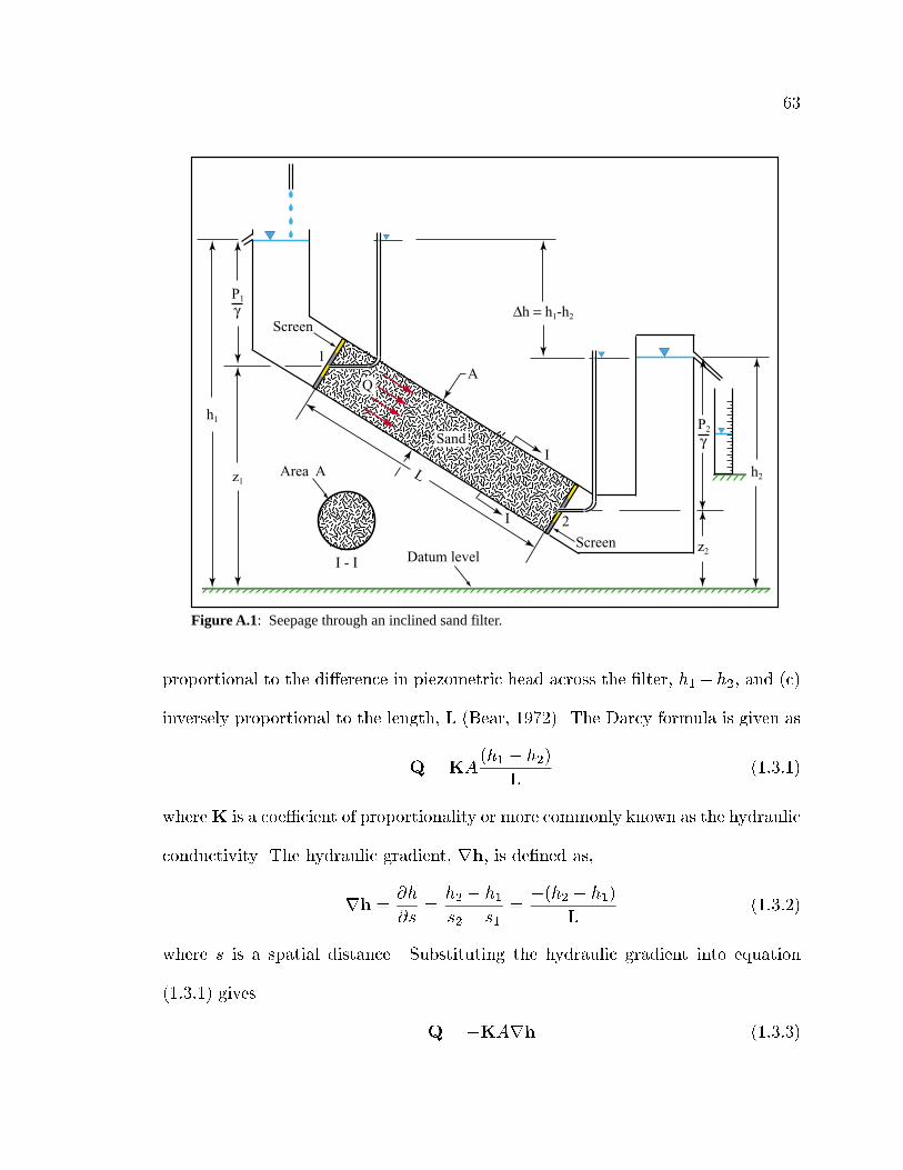
63

Figure A.1: Seepage through an inclined sand filter.

I - I

1

2

L

I

I

∆h = h1-h2

h2

P2

γ

z2

P1

γ

z1

h1

Area A

AQ

Datum level

Sand

Screen

Screen

proportional to the dierence in piezometric head across the lter, h1 h2, and (c)

inversely proportional to the length, L (Bear, 1972). The Darcy formula is given as

Q = KA(h1 h2)

L(1:3:1)

whereK is a coecient of proportionality or more commonly known as the hydraulic

conductivity. The hydraulic gradient, rh, is dened as,

rh =@h

@s=

h2 h1

s2 s1=(h2 h1)

L(1:3:2)

where s is a spatial distance. Substituting the hydraulic gradient into equation

(1:3:1) gives

Q = KArh (1:3:3)

64

The specic discharge, q, is dened as the discharge per unit cross-sectional area

normal to the direction of ow.

q =Q

A

:=

L

T

(1:3:4)

Substituting q into Equation (1:3:3) gives

q = Krh (1:3:5)

where

rh =@h

@s=

dh

dxi+

dh

dyj+

dh

dzk (1:3:6)

and i, j, k are unit vectors in the x,y,z coordinate directions, respectively.

The functional relationship between hydraulic head, h, and uid pressure, p, is

dened as

h =

Zp

p0

dp

+

v2

2g+ z (1:3:7)

where is the specic weight of water, v, is the average uid velocity, and z is the

vertical distance above an established datum. It is assumed that changes in piezo-

metric head, h, are much larger than changes in the kinetic energy head along the

ow path. Fluid velocities are assumed insignicant when compared with the pres-

sure and elevation terms in Equation (1:3:8). Therefore, kinetic energy is neglected

when considering the head loss along the ow path.

h =

Zp

p0

dp

+ z (1:3:8)

or

rh =rp

+rz (1:3:9)

65

For cases where density or viscosity are not constant, SUTRA utilizes a simplied

version of the hydraulic conductivity,

K =cd

2

=kkr

(1:3:10)

where c is the shape factor and d is the mean grain diameter. Both c and d are based

on the properties of the porous media. Fluid velocity, even for a given pressure and

density distribution, may take on dierent values depending on how mobile the

uid is within the solid matrix. Fluid mobility depends on the combination of

permeability, k, relative permeability, kr, and dynamic viscosity, . Permeability

is a measure of the ease of uid movement through interconnected voids in the

isotropic solid matrix when all voids are completely saturated. Relative permeability

expresses the fraction of the total permeability remaining when the voids are only

partly uid-lled and only part of the total interconnected void space is connected

by continuous uid channels. SUTRA assumes kr to be independent of direction in

the isotropic porous media.

Returning to Equation (1:3:6), Darcy's law is further developed.

q = Krh =

kkr

rp

+rz

=kkr

rp+ rz

(1:3:11)

The average uid velocity, v, is the velocity of uid with respect to the stationary

solid matrix. By denition, the specic discharge, q, is

q = Swv

8void

8total

8water

8void

v

:=

L

T

(1:3:12)

Substituting for q in Equation (1:3:12) gives

Swv=kkr

rp+ rz

66

v=kkr

Sw

rp+ grz

(1:3:13)

The gravity vector is dened in relation to the direction in which vertical elevation

is measured

g= jgjrz ) g =

grz

(1:3:14)

where gis the magnitude of the gravitational acceleration vector. Substituting g

into Equation (1:3:14) gives the average velocity as

v=

kkr

Sw

rp g

(1:3:15)

A functional relationship between permeability and pressure is required by

SUTRA within the UNSAT subroutine. A general function of kr(p), will be used

and is given within the Unsaturated Conditions section of this report.

1.4 Partially Saturated Conditions:

A predictive model is used to describe the movement of groundwater within

partially saturated conditions (negative pressure elds). The model is specically

used to predict the relative permeability of unsaturated soils for a given water

pressure. To derive the relative permeability in the unsaturated state, the model

makes use of the measured pressure head versus water saturation curve, p(Sw). The

models development, as outlined by Mualem (1976), is presented below.

Consider a homogeneous porous medium having interconnected pores dened

by their radius r. Pores within the medium, at complete saturation, go from a radius

of r to r + dr. The change in radii, r ! r + dr, within the full pores contributes

67

to a change in water saturation. If f(r) is the pore water distribution function, the

contribution to Sw is

f(r)dr = dSw (1:4:1)

Integration over the pore radii gives water saturation as a function of the pore radius

Zr

rmin

f(r)dr = Sw(r) (1:4:2)

and for saturated conditions,

Zrmax

rmin

f(r)dr = Ssat (1:4:3)

The areal porosity, Avoid

Atotal

, is equal to the volumetric porosity, 8void

8total, so f(r)dr repre-

sents the ratio between the pore area of radii r! r+dr and the total area (Mualem,

1976).

Consider a conceptual soil structure, Figure A.2, where a porous slab of thick-

ness x hypothetically isolates a homogeneous soil column. The pore area distribu-

tion for the two slab sides is identical and equal to f(r)dr. For x much larger than

the maximum radius, x >> rmax, complete randomness of the relative position of

the voids at the two slab faces would exist. The independence of pore distributions

at x and x+x implies that their probability for intersecting is

dAe =f(r1)dr1

f(r2)dr2

= f(r1)f(r2)dr1dr2 (1:4:4)

where dAe is both the change in pore area and the probability that a pore of radius

r1 nds a pore of radius r2 when moving over a distance of x. For 0 x < rmax

there exists a correlation between r1 and r2 with perfect correlation at x = 0. To

68

account for the degree of correlation between the two sides, the change in pore area,

dAe, is rewritten with a dependency on water saturation, Sw,

dAe = Su2w

f(r1)f(r2)dr1dr2 (1:4:5)

where u describes the connectivity of the pore structure. The parameter u ranges

from u = 1 for full correlation to u = 2 for no correlation. For a given water

saturation, integration of Equation (1:4:5) over the range of radii of the water-lled

pores is

Ae =

Zrmax

rmin

dAe =

Zrmax

rmin

Zrmax

rmin

Su2w

f(r1)f(r2)dr1dr2 (1:4:6)

0 < ∆x < rmax∆x >> rmax ∆x = 0

Partial Correlation between r1 and r2

Perfect Correlation between r1 and r2

No Correlation (Independent) between r1 and r2

r1 r2

x x+∆x x x+∆x x

Figure A.2: Variations of ∆x within a conceptual soil structure. Homogeneous soil with pore area distributions identical at the two slab sides, (1) & (2).

soilporous slab soil

The contribution of the actual ow conguration in the slab to the hydraulic

conductivity, K, requires two simplifying assumptions: (1) there is no bypass ow

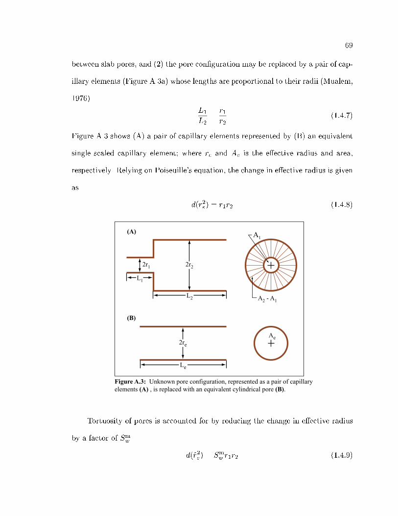
69

between slab pores, and (2) the pore conguration may be replaced by a pair of cap-

illary elements (Figure A.3a) whose lengths are proportional to their radii (Mualem,

1976).

L1

L2=

r1

r2(1:4:7)

Figure A.3 shows (A) a pair of capillary elements represented by (B) an equivalent

single scaled capillary element; where re and Ae is the eective radius and area,

respectively. Relying on Poiseuille's equation, the change in eective radius is given

as

d(r2e) = r1r2 (1:4:8)

A1

2r1 2r2

L2

L1

Le

2re

Ae

A2 - A1

(A)

(B)

Figure A.3: Unknown pore configuration, represented as a pair of capillaryelements (A) , is replaced with an equivalent cylindrical pore (B).

Tortuosity of pores is accounted for by reducing the change in eective radius

by a factor of Smw.

d(r2e) = S

m

wr1r2 (1:4:9)

70

Darcy's Law (Equation 1.3.3) applied to the equivalent tube (Figure A.3b) yields

Q = KArh =

cd2

(Ae Asat)rh (1:4:10)

where the eective area is given as

Ae =A

Asat

) A = Ae Asat (1:4:11)

where Asat is the pore area at saturation. Darcy's Law in terms of the specic

discharge, q, is given as

q =

cd2

Aerh =

c

d2Aerh

= Md2Aerh = (Mr2eAe)rh (1:4:12)

where M = c

is a constant which incorporates properties of the uid and solid

matrix. The eective radius, re, is assumed equal to mean grain diameter, d. The

changes in ux resulting from the contribution of full pores going from r to r + dr

is

dq = dMr2

eAerh

= Mdr2

edAerh (1:4:13)

Integrating the specic discharge over the water lled pores gives

q =

Zdq =

M0

Zwater lled pores

dr2edAe

rh (1:4:14)

which allows K to be isolated from the modied form of Darcy's Law (Equation

1:4:14).

K = M0

Zwater lled pores

dr2edAe (1:4:15)

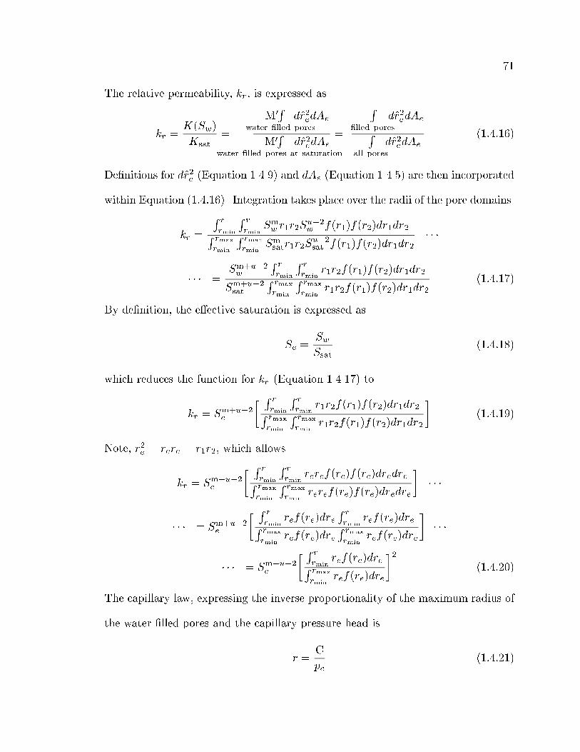
71

The relative permeability, kr, is expressed as

kr =K(Sw)

Ksat

=

M0R

water lled pores

dr2edAe

M0

Rwater lled pores at saturation

dr2edAe

=

Rlled pores

dr2edAe

Rall pores

dr2edAe

(1:4:16)

Denitions for dr2e(Equation 1.4.9) and dAe (Equation 1.4.5) are then incorporated

within Equation (1:4:16). Integration takes place over the radii of the pore domains.

kr =

Rr

rmin

Rr

rmin

Sm

wr1r2S

u2

wf(r1)f(r2)dr1dr2R

rmax

rmin

Rrmax

rmin

Sm

satr1r2S

u2

satf(r1)f(r2)dr1dr2

=Sm+u2

w

Rr

rmin

Rr

rmin

r1r2f(r1)f(r2)dr1dr2

Sm+u2

sat

Rrmax

rmin

Rrmax

rmin

r1r2f(r1)f(r2)dr1dr2(1:4:17)

By denition, the eective saturation is expressed as

Se =Sw

Ssat(1:4:18)

which reduces the function for kr (Equation 1.4.17) to

kr = Sm+u2

e

Rr

rmin

Rr

rmin

r1r2f(r1)f(r2)dr1dr2Rrmax

rmin

Rrmax

rmin

r1r2f(r1)f(r2)dr1dr2

(1:4:19)

Note, r2e= rere = r1r2, which allows

kr = Sm+u2

e

Rr

rmin

Rr

rmin

reref(re)f(re)dredreRrmax

rmin

Rrmax

rmin

reref(re)f(re)dredre

= Sm+u2

e

Rr

rmin

ref(re)dreRr

rmin

ref(re)dreRrmax

rmin

ref(re)dreRrmax

rmin

ref(re)dre

= Sm+u2

e

Rr

rmin

ref(re)dreRrmax

rmin

ref(re)dre

2(1:4:20)

The capillary law, expressing the inverse proportionality of the maximum radius of

the water lled pores and the capillary pressure head is

r =C

pc(1:4:21)

72

where C is a proportionality constant. Expressing kr in terms of p and substituting

for f(re)dr = dSe from Equation (1:4:1) yields

kr = Sm+u2e

RSe

0

C

pc

dSeR

Ssat

0

C

pc

dSw

2

= Sm+u2e

RSw

0

1

pc

dSeR

Ssat

0

1

pc

dSe

2

(1:4:22)

Since there exists no procedure for an independent determination of m, the

eects of tortuosity, and u, the correlation factors, both m and u are lumped together

into a single parameter n.

n = m+ u 2 (1:4:23)

The parameter n is determined from a curve tting technique between kr(pc) in

Equation (1:4:22) and the empirical relation of krm(pc) found through experiment.

For each soil the mean square deviation, D, between krm and kr is

D =

Z1

Se min

[ln(kr) ln(krm)]2

(1 Se min)dSe

1

2

(1:4:24)

Posing the problem as a parameter estimation optimization gives the objective as

the minimization of the error between measured and computed permeability while

treating n as the decision variable. The problem associated with this technique is

the dependency of n on the specic soil type being used. A general n value which

could be used for all soils was determined by Mualem (1976). In order to maintain

consistency in the numerical computation of D for all soils, Mualem solved for a

mean value of D based on 45 common soils. Each of the 45 soils are cited within

the literature and contain measured p-Se and K-Sw data on drainage. Holding n

constant, a D value is calculated. The magnitude of D represents the performance

of n in characterizing the 45 soils. Mualem's results, Figure A.4, show an optimal

solution of n = 1

2.

73

-1.0 -0.5 0.0 0.5 1.0 1.5 2.0 2.50.6

1.0

1.6

0.8

1.2

1.4

1.8

2.0

n

D

Figure A.4: Computed D based on 45 soils as a function of the power n (Mualem, 1976).

To solve Equation (1:4:22), an expression relating the dimensionless saturation

or eective saturation, Se, to the capillary pressure, pc, is needed. The functional

relationship, Se(pc), adopted for this study was established by van Genuchten (1980)

and is given in its general form as

Se =

1

1 + (apc)n

m

(1:4:25)

where a, n, and m are parameters dependent on the materials within the study site.

Solving for the capillary pressure, pc, within Equation (1:4:25), yields

S

1

m

e =1

1 + (apc)n) (apc)

n =1

S

1

m

e

1 )

apc =

1

S

1

m

e

1

n

) pc =1

a

1 S

1

m

e

S

1

m

e

1

n

(1:4:26)

Equation (1:4:22) is further developed with the capillary pressure denition given

74

in Equation (1:4:26). A substitution for n = 12is made.

kr(Se) = S

1

2

e

"RSe

01pc

dSeR 1

01pc

dSe

#2= S

1

2

e

f(Se)

f(Se;sat)

2(1:4:27)

where

f(Se) =

ZSe

0

1

pc

dSe =

ZSe

0

1

1a

1S

1

m

e

S

1

m

e

1

n

dSe

= a

ZSe

0

S

1

m

e

1 S

1

m

e

1

n

dSe (1:4:28)

The relative permeability, kr, is assumed a power function of the eective saturation,

Se. Substitution of Se = Sm into Equation (1:4:28) leads to

f(S) = a

ZSe

1

m

0

(Sm)

1

m1 (Sm)

1

2

1

n

d

S

m

= a

ZSe

1

2

0

S

1

n

(1 S)1

n

mS

m1dS = am

ZSe

1

m

0

S

m1+ 1

n (1 S)1

ndS

= am

ZSe

1

m

0

S

k(1 S)1

ndS (1:4:29)

where m is limited to (0 < m < 1). In it's most general form, no closed-form

expression can be derived for Equation (1:4:29). However, integration is possible

for all integer values of k, where k = m 1+ 1n. For the particular case when k = 0

(i.e. m = n1n

and 1n= 1m), integration of Equation (1:4:29) gives

f(S) = am

ZSe

1

m

0

S

m1+(1m)(1 S)(1m)dS

= am

ZSe

1

2

0

S

0(1 S)m1 dS

75

= am

(1 S)m

m

S 1

2e

0

= a

(1 S

1

m

e )m 1

(1:4:30)

Equation (1:4:29) in terms of the eective saturation, Se, and the eective saturation

at saturation, Se;sat, is

f(Se) = a

(1 S

1

m

e )m 1

(1:4:31)

f(Se;sat) = a

(1 1

1

m )m 1= a (1:4:32)

which allows Equation (1:4:27) to be written as,

kr(Se) = S

1

2

e

"a(1 S

1

m

e )m 1

a

#2= S

1

2

e

1 (1 S

1

m

e )m2

(1:4:33)

Substituting the eective saturation, Se, found in Equation (1:4:25), into Equation

(1:4:32) gives the relative permeability as a function of capillary pressure, kr(pc).

kr(pc) =

1

1 + (apc)n

m2

1

1

1

1 + (apc)n

mm

m2

=

"1

1 + (apc)nm

2

#1

1 (apc)

n 1

1 + (apc)n

m2

=

1 (apc)

nm1 + (apc)

nm2

1 + (apc)n

m2

(1:4:34)

where

m = 11

n(1:4:35)

when k = 0. The dimensionless saturation, Se is dened as

Se =Sw Swres

Ssat Swres

(1:4:36)

76

where Swres is a residual saturation below which saturation is not expected to fall.

Water becomes immobile for Sw < Swres. Equation (1:4:25) in terms of the residual

saturation is given as

Sw = Swres + (Ssat Swres)

1

1 + (apc)n

m

(1:4:37)

Substituting for m in Equation (1:4:37) gives the water saturation as a function of

capillary pressure, pc.

Sw(pc) = Swres + (Ssat Swres)

1

1 + (apc)n

n1n

= Swres + (1 Swres)1 + (apc)

n 1nn (1:4:38)

Steps taken for the derivation of Sw with respect to p are as follows:

dSw

dp=

Ssat Swres

1 n

n

1 + (a(p))n

([ 1nn

]1)

(n)(a(p))n1(a)(1)

=Ssat Swres

n 1

n

1 + (a(p))n

(

2n1

n)(n)(a(p))n1(a)

=(a)(n 1)(Ssat Swres)(a(p))

n1

1 + (a(p))n

2n1n

(1:4:39)

where p = pc. The user-programmed subroutine UNSAT, located within SUTRA,

requires (A) water saturation as a function of pressure, (B) the derivative of satu-

ration with respect to pressure, and (C) the relative permeability as a function of

pressure. The three required conditions are given below:

Sw(p) = Swres + (Ssat Swres)1 + (ajpj)n

m

(1:4:40)

dSw

dp=

(a)(n 1)(Ssat Swres)(ajpj)n1

1 + (ajpj)n

2n1n

(1:4:41)

kr(p) =

1 (ajpj)n1

1 + (ajpj)n

m

21 + (ajpj)n

m2

(1:4:42)

77

where m = 1 1=n and p < 0. Functions (A) and (C) are presented graphically in

Figures A.5 and A.6, respectively. Unsaturated parameter values are based upon

physical properties identied for Webster clay loam: a ne-loamy, mixed, superac-

tive, mesic, Typic Endoaquoll, 32% sand, 39% silt, and 28% clay (Shao and Horton,

1998).

0

0.1

0.2

0.3

0.4

0.5

0.6

a = 0.0125 cm-1

n = 1.38

Swres = 0.07Ssat = 0.56

Satu

ratio

n, S

w

Figure A.6: Relative permeability versus pressure.

Figure A.5: Water saturation versus pressure.

1E-18

1E-16

1E-14

1E-12

1E-10

1E-08

1E-06

1E-04

1E-02

1E+00 a = 0.0125 cm-1

n = 1.38

Rel

ativ

e Pe

rmea

bilit

y, k

r

Pressure, p [cm]

Pressure, p [cm]-1.0 -1E+1 -1E+2 -1E+3 -1E+4 -1E+5 -1E+6 -1E+7

-1.0 -1E+1 -1E+2 -1E+3 -1E+4 -1E+5 -1E+6 -1E+7

78

1.5 Fluid Mass Balance:

Simulation of ow within SUTRA is nothing more than a calculation of how the

amount of uid mass contained within the void spaces of the solid matrix changes

with time. A uid mass balance is used to keep track of the uid mass held at

every point in the simulated groundwater system as it changes with time due to

ows and saturation changes. The continuity equation for the groundwater system

is developed by considering a nondeforming elemental volume located within the

aquifer (Figure A.7). The principle of mass conservation requires,

Mass

in ow rate

Mass

out ow rate

=Time rate of change

in mass storage

(1:5:1)

or

IO =@M

@t

(1:5:2)

The mass ow rate through an elemental area is qnA where qn is the compo-

nent of the mean seepage uid velocity normal to the surface of an element of area

A. Assuming that the volume is completely saturated with a single-phase, homoge-

neous uid of density , and the mean seepage velocity of the uid and density are

given at point P, the centroid of the control volume, then a Taylor series expansion

about point P is used to obtain the net mass in ow to the elemental volume (Willis

and Yeh, 1987). For example, the mass in ow in the x direction, Ix, is

Ix = qxyz

@

@x

(qx)x

2yz

:

=

M

T

(1:5:3)

Similarly, the mass out ow in the x direction, Ox, is

Ox = qxyz +@

@x

(qx)x

2yz

:

=

M

T

(1:5:4)

79

Figure A.7: Mass conservation for a control volume.

y

x

z

Iz|x,y,z- δz2

Oz|x,y,z+δz2

Oy|x,y+ ,zδy2

Ox|x+ ,y,zδx2

Iy|x,y- ,zδy2

Ix|x- ,y,zδx2 P

δy

δz

δx

Summing the contributions to the in ow and out ow in the x direction gives,

Ix Ox = qxyz @

@x(qx)

x

2yz qxyz

@

@x(qx)

x

2yz

=

@

@x(qx)xyz (1:5:5)

Summing the contributions to the in ow and out ow in the x,y,z directions, the

net mass in ow is

IO =

@

@x(qx)xyz

@

@y(qy)xyz

@

@z(qz)xyz

IO =

@

@x(qx) +

@

@y(qy) +

@

@z(qz)

xyz (1:5:6)

or in vector notation,

IO = (r q)xyz (1:5:7)

80

where r is the divergence operator,

r =@

@xi+

@

@yj+

@

@zk

The net increase in the mass ow rate is equal to the rate of change of the mass

stored within the elemental volume. The mass M of the uid contained in the

volume is

M = Swxyz

8void

8total

8water

8void

Mass

8water

8total Mass (1:5:8)

The time rate of change in mass storage is given as

@M

@t=

@

@t(Sw)xyz

:=

M

T

(1:5:9)

The continuity Equation (1:5:2) for the groundwater system is then expressed as,

(r q)xyz =@

@t(Sw)xyz (1:5:10)

r q =@

@t(Sw) (1:5:11)

Substituting q = Swvfrom Equation (1:3:13) gives

r (Swv) =

@(Sw)

@t(1:5:12)

A uid mass source term, Qp, is added to Equation (1:5:12) to account for external

additions of uid mass (e.g. a precipitation input).

@(Sw)

@t= r (Swv

) +Qp (1:5:13)

where

Qp

:=

M

L3T

81

From Equation (1:2:8) the time rate of change in mass storage is dened as

@(Sw)

@t

=

Sw

@()

@p

+

@(Sw)

@p

@p

@t

=

SwSop +

@(Sw)

@p

@p

@t

(1:5:14)

which allows Equation (1:5:13) to be written as

SwSop +

@(Sw)

@p

@p

@t

= r (Swv) +Qp (1:5:15)

Substituting in the denition for average velocity, v, Equation (1:5:15) becomes

SwSop +

@(Sw)

@p

@p

@t

= r

(Sw)

kkr

Sw

rp g

+Qp (1:5:16)

or SwSop +

@Sw

@p

@p

@t

r

kkr

rp g

= Qp (1:5:17)

APPENDIX B: Numerical Methods

The model employs a two-dimensional hybrid nite-element and integrated-

nite-dierence method to approximate the governing equation that describes uid

density dependent saturated or unsaturated groundwater ow. The following sec-

tions review the numerical methods used by SUTRA. The numerical tools required

for the approximation of the uid mass balance are basis functions, coordinate

transformations, and Gaussian integration.

2.1 Basis Functions:

In a nite-element analysis, the dependent variables (e.g. pressure) are approx-

imated by polynomial functions that are dened in terms of the unknown nodal

values of the state or dependent variables. These approximating or interpolating

functions vary over each element of the system, although continuity of the func-

tion is maintained along the element boundaries (Willis and Yeh, 1987). Linear

basis functions are used by SUTRA to described the unknown nodal values over

the system of two-dimensional quadrilateral elements.

Integration of linear basis functions is required within the model formulation.

Basis functions are developed within a local coordinate system to facilitate the

integration. Figure B.1 illustrates an element in both the global and local coordinate

systems. The irregularly shaped element within the global coordinate system, (x; z),

is reduced to a square in the local coordinate system, (; ). Furthermore, the square

in (; ) has its corners (nodes) located at = 1, = 1. The relation between

82

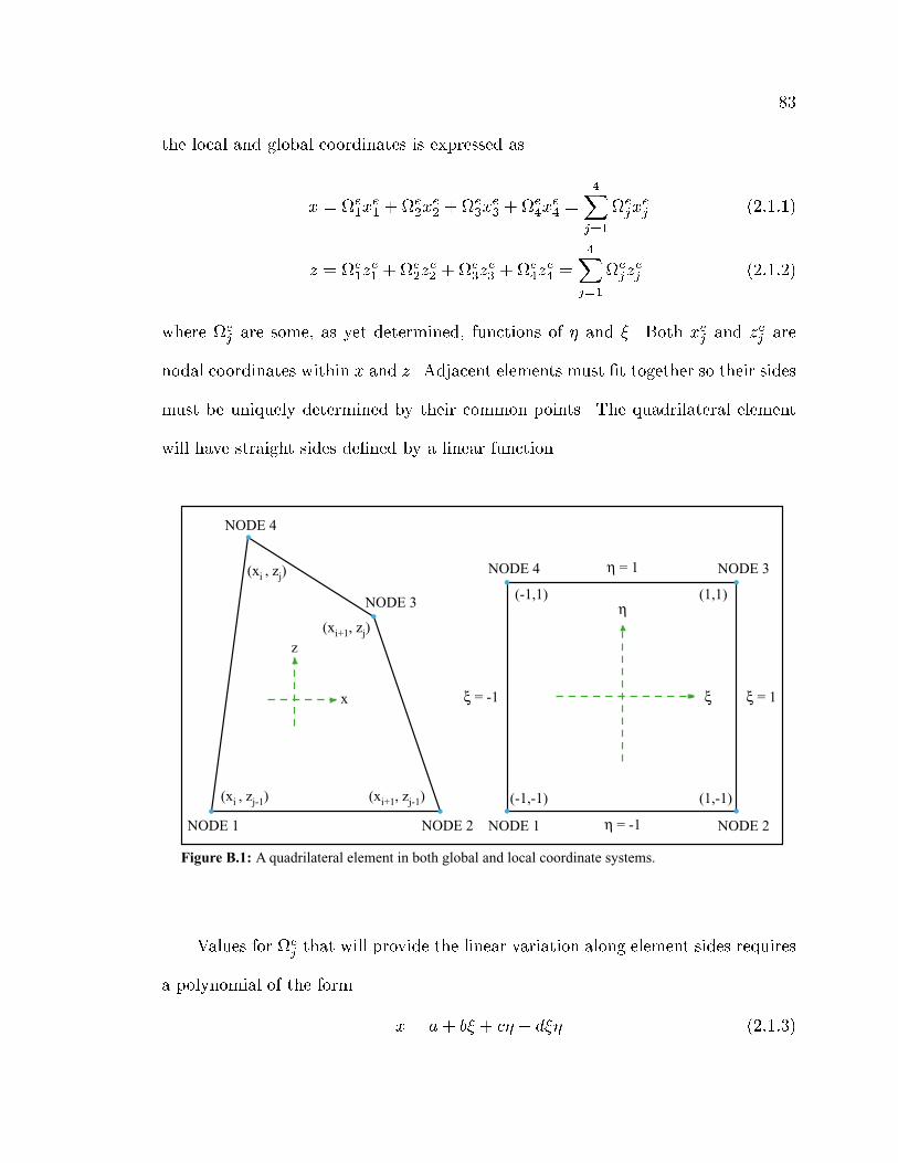
83

the local and global coordinates is expressed as

x = e

1xe

1+ e

2xe

2+ e

3xe

3+ e

4xe

4=

4X

j=1

e

jxe

j(2:1:1)

z = e

1ze

1+ e

2ze

2+ e

3ze

3+ e

4ze

4=

4X

j=1

e

jze

j(2:1:2)

where e

jare some, as yet determined, functions of and . Both x

e

jand z

e

jare

nodal coordinates within x and z. Adjacent elements must t together so their sides

must be uniquely determined by their common points. The quadrilateral element

will have straight sides dened by a linear function.

Figure B.1: A quadrilateral element in both global and local coordinate systems.

ξ

η

NODE 4 NODE 3

NODE 1 NODE 2

(-1,1) (1,1)

(-1,-1) (1,-1)

NODE 1

NODE 4

NODE 2

NODE 3

x

z

(xi+1, zj-1)(xi , zj-1)

(xi , zj)

(xi+1, zj)

η = 1

η = -1

ξ = 1ξ = -1

Values for e

jthat will provide the linear variation along element sides requires

a polynomial of the form

x = a+ b + c + d (2:1:3)

84

which is linear in when = 1 and linear in when = 1. We also have, from

Figure B.1, the following conditions,

x = x1 when = = 1 (2:1:4)

x = x2 when = 1; = 1

x = x3 when = = 1

x = x4 when = 1; = 1

Substituting these constraints into Equation (2:1:3) gives

8><>:

x1x2x3x4

9>=>;

=

2641 1 1 111 2 2 221 3 3 311 4 4 44

375

8><>:

a

b

c

d

9>=>;

=

2641 1 1 1

1 1 1 1

1 1 1 1

1 1 1 1

375

8><>:

a

b

c

d

9>=>;

(2:1:5)

or, in vector-matrix notation

x =A

P

(2:1:6)

P =A

1

x

(2:1:7)

where

A

1

=1

4

264

1 1 1 1

1 1 1 1

1 1 1 1

1 1 1 1

375 (2:1:8)

Substituting P into the matrix form of Equation (2:1:5) yields,

x =1

8><>:

a

b

c

d

9>=>;

=1

P =

1

A

1

x

(2:1:9)

A comparison of Equation (2:1:1) and (2:1:9) reveals,

x =eT

xe=1

A

1

x

(2:1:10)

85

or

eT

=1

A1

2641

2

3

4

375 =

1

1

4

2641 1 1 1

1 1 1 1

1 1 1 1

1 1 1 1

375 (2:1:11)

where

1 =1

4(1 + ) =

1

4(1 )(1 ) (2:1:12)

2 =1

4(1 + ) =

1

4(1 + )(1 ) (2:1:13)

3 =1

4(1 + + + ) =

1

4(1 + )(1 + ) (2:1:14)

4 =1

4(1 + ) =

1

4(1 )(1 + ) (2:1:15)

Figure B.2 illustrates the basis function dened over a four element local space.

Nodes are described with global coordinates to help facilitate the connection be-

tween local and global coordinate systems. The basis function within the local

coordinate system is given as e(i; j), while (xi; yj) is given for the basis func-

tion within the global coordinate system. One basis function is dened for each

node.

Figure B.3 illustrates multiple perspectives of the basis function, j , dened

for node j. The basis function has a value of one at node j and a value of zero at

all other nodes. The surface representing j over an element is curved due to the

product of and in Equation (2:1:11).

The derivatives of the bi-linear basis functions which depend on only one space

coordinate are given as:

@1

@=

@

@

1

4

4

4+

4

=

1

4+

4=

1

4(1 ) (2:1:16)

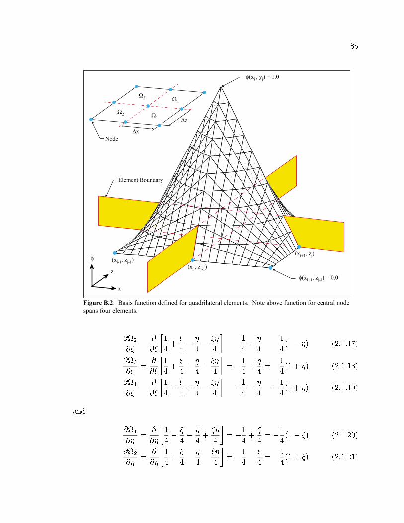
86

x

z

φ

φ(xi+1, zj-1) = 0.0

(xi-1, zj-1)(xi , zj-1)

(xi+1, zj)

φ(xi , yj) = 1.0

Figure B.2: Basis function defined for quadrilateral elements. Note above function for central nodespans four elements.

Element Boundary

Node

Ω1Ω2

Ω4Ω3

∆x

∆z

@2

@=

@

@

1

4+

4

4

4

=

1

4

4=

1

4(1 ) (2:1:17)

@3

@=

@

@

1

4+

4+

4+

4

=

1

4+

4=

1

4(1 + ) (2:1:18)

@4

@=

@

@

1

4

4+

4

4

=

1

4

4=

1

4(1 + ) (2:1:19)

and

@1

@=

@

@

1

4

4

4+

4

=

1

4+

4=

1

4(1 ) (2:1:20)

@2

@=

@

@

1

4+

4

4

4

=

1

4

4=

1

4(1 + ) (2:1:21)

87

0.0

0.1

0.2

0.3

0.4

0.5

0.6

0.7

0.8

0.9

1.00.9-1.0

0.8-0.9

0.7-0.8

0.6-0.7

0.5-0.6

0.4-0.5

0.3-0.4

0.2-0.3

0.1-0.2

0.0-0.1

(-1,-1)

(1,1)

(-1,1)

(1,-1)ξ

η

Ωj

node j

0.0

0.1

0.2

0.3

0.4

0.5

0.6

0.7

0.8

0.9

1.0

(-1,-1) (1,1)node j ξ and η

Ωj

Figure B.3: Perspectives of basis function Ωj(ξ,η) at node j.

88

@3

@=

@

@

1

4+

4+

4+

4

=

1

4+

4=

1

4(1 + ) (2:1:22)

@4

@=

@

@

1

4

4+

4

4

=

1

4

4=

1

4(1 ) (2:1:23)

2.2 Coordinate Transformations:

Coordinate transformation between local, (; ), and global, (x; z), coordinate

systems is required for the nite-element mesh calculations and integral evaluations.

The transformation involves a linear remapping in each coordinate direction and

employs the basis functions, j , to provide mapping. The ability to map from

one coordinate system to another is based on the chain rule of dierentiation. For

functions of two variables, we have,

@j

@=

@j

@x

@x

@+

@j

@z

@z

@(2:2:1)

@j

@=

@j

@x

@x

@+

@j

@z

@z

@(2:2:2)

In matrix notation, equations (2:2:1) and (2:2:2) are combined to give transforma-

tions for both directions local to global and global to local.(@j

@@j

@

)=

@x@

@z@

@x@

@z@

@j

@x@j

@z

= J

@j

@x@j

@z

(2:2:3)

and @j

@x@j

@z

=

@x@

@z@

@x@

@z@

1(

@j

@@j

@

)= J

1

@j

@x@j

@z

(2:2:4)

where

J =

J11 J12J21 J22

=

@x@

@z@

@x@

@z@

(2:2:5)

J1 =

1

det J

J22 J12

J21 J11

=

1

J11J22 J12J21

J22 J12

J21 J11

=

1

@x@

@z@

@z@

@x@

@z@

@z@

@x@

@x@

(2:2:6)

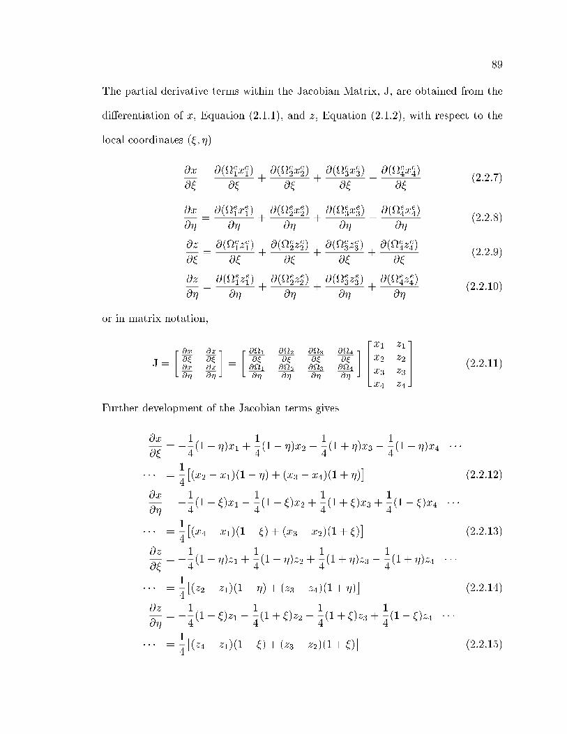
89

The partial derivative terms within the Jacobian Matrix, J, are obtained from the

dierentiation of x, Equation (2:1:1), and z, Equation (2:1:2), with respect to the

local coordinates (; ).

@x

@=

@(e

1xe

1)

@+

@(e

2xe

2)

@+

@(e

3xe

3)

@+

@(e

4xe

4)

@(2:2:7)

@x

@=

@(e

1xe

1)

@+

@(e

2xe

2)

@+

@(e

3xe

3)

@+

@(e

4xe

4)

@(2:2:8)

@z

@=

@(e

1ze

1)

@+

@(e

2ze

2)

@+

@(e

3ze

3)

@+

@(e

4ze

4)

@(2:2:9)

@z

@=

@(e

1ze

1)

@+

@(e

2ze

2)

@+

@(e

3ze

3)

@+

@(e

4ze

4)

@(2:2:10)

or in matrix notation,

J =

@x

@

@z

@

@x

@

@z

@

=

@1

@

@2

@

@3

@

@4

@

@1

@

@2

@

@3

@

@4

@

264x1 z1

x2 z2

x3 z3

x4 z4

375 (2:2:11)

Further development of the Jacobian terms gives

@x

@=

1

4(1 )x1 +

1

4(1 )x2 +

1

4(1 + )x3

1

4(1 + )x4

=1

4

(x2 x1)(1 ) + (x3 x4)(1 + )

(2:2:12)

@x

@=

1

4(1 )x1

1

4(1 + )x2 +

1

4(1 + )x3 +

1

4(1 )x4

=1

4

(x4 x1)(1 ) + (x3 x2)(1 + )

(2:2:13)

@z

@=

1

4(1 )z1 +

1

4(1 )z2 +

1

4(1 + )z3

1

4(1 + )z4

=1

4

(z2 z1)(1 ) + (z3 z4)(1 + )

(2:2:14)

@z

@=

1

4(1 )z1

1

4(1 + )z2 +

1

4(1 + )z3 +

1

4(1 )z4

=1

4

(z4 z1)(1 ) + (z3 z2)(1 + )

(2:2:15)

90

In addition to transforming the derivatives from (x; z) to (; ), the area of the

element is changed using

dA = dxdz = (det J)dd (2:2:16)

Integrating over each element within the local coordinate system gives

A =

ZdA =

Zz

Zx

dxdz =

Z1

1

Z1

1

(det J)dd (2:2:17)

2.3 Gaussian Integration:

Gaussian quadrature is a technique for solving the exact integration of poly-

nomials through the summation of the integrands' point values. Integration is

performed by replacing a denite integral with a nite series. The symbolic form

of Gaussian integration is,

Z=1

=1

f()d =

npXgp=1

Hgpf(gp) (2:3:1)

where f() is the function to be integrated between = 1 to = +1, gp is

the Gauss point number, np is the total number of Gauss points, and Hgp are the

weighting coecients.

In order to integrate a term of the dierential governing equation, f(x; z),

over an arbitrary quadrilateral element, the limits of the integral must rst be

transformed to local coordinate values of 1 to +1.

Zz

Zx

f(x; z)dxdz =

Z

Z

f(; )(det J)dd =

Z1

1

Z1

1

~f(; )dd (2:3:2)

91

Gaussian integration is applied independently to each integral with two Gauss points

required for each coordinate direction. The Gauss point values for numbers one and

two are 31

2 and +31

2 respectively.

Zz

Zx

f(x; z)dxdz =

Z1

1

"2X

i=1

~f(i; )

#d =

2Xj=1

2Xi=1

~f(i; j) (2:3:3)

Identical limits of integration for the two integrals allows for a single summation of

Equation (2:3:3). Zz

Zx

f(x; z)dxdz =

4Xgp=1

~f(gp; gp) (2:3:4)

where each of the four Gauss point values are shown in Figure B.4.

Figure B.4: Finite element in local coordinate system with Gauss points.

ζ

η

NODE 4 NODE 3

NODE 1 NODE 2

(-1,1) (1,1)

(-1,-1) (1,-1)

GAUSS POINT 2

(0.577,-0.577)

GAUSS POINT 3

(0.577,0.577)

GAUSS POINT 4

(-0.577,0.577)

GAUSS POINT 1

(-0.577,-0.577)

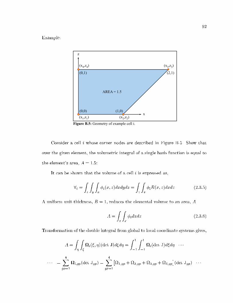
92

Example:

Figure B.5: Geometry of example cell i.

x

z

(1,0)(0,0)

(0,1) (2,1)

AREA = 1.5

(x1,z1) (x2,z2)

(x3,z3)(x4,z4)

Consider a cell i whose corner nodes are described in Figure B.5. Show that

over the given element, the volumetric integral of a single basis function is equal to

the element's area, A = 1:5:

It can be shown that the volume of a cell i is expressed as,

8i =

Zz

Zy

Zx

i(x; z)dxdydz =

Zz

Zx

iB(x; z)dxdz (2:3:5)

A uniform unit thickness, B = 1, reduces the elemental volume to an area, A.

A =

Zz

Zx

idxdz (2:3:6)

Transformation of the double integral from global to local coordinate systems gives,

A =

Z

Z

i(; )(det J)dd =

Z1

1

Z1

1

i(det J)dd

=

4Xgp=1

i;gp(det Jgp) =

4Xgp=1

1;gp + 2;gp + 3;gp + 4;gp

(det Jgp)

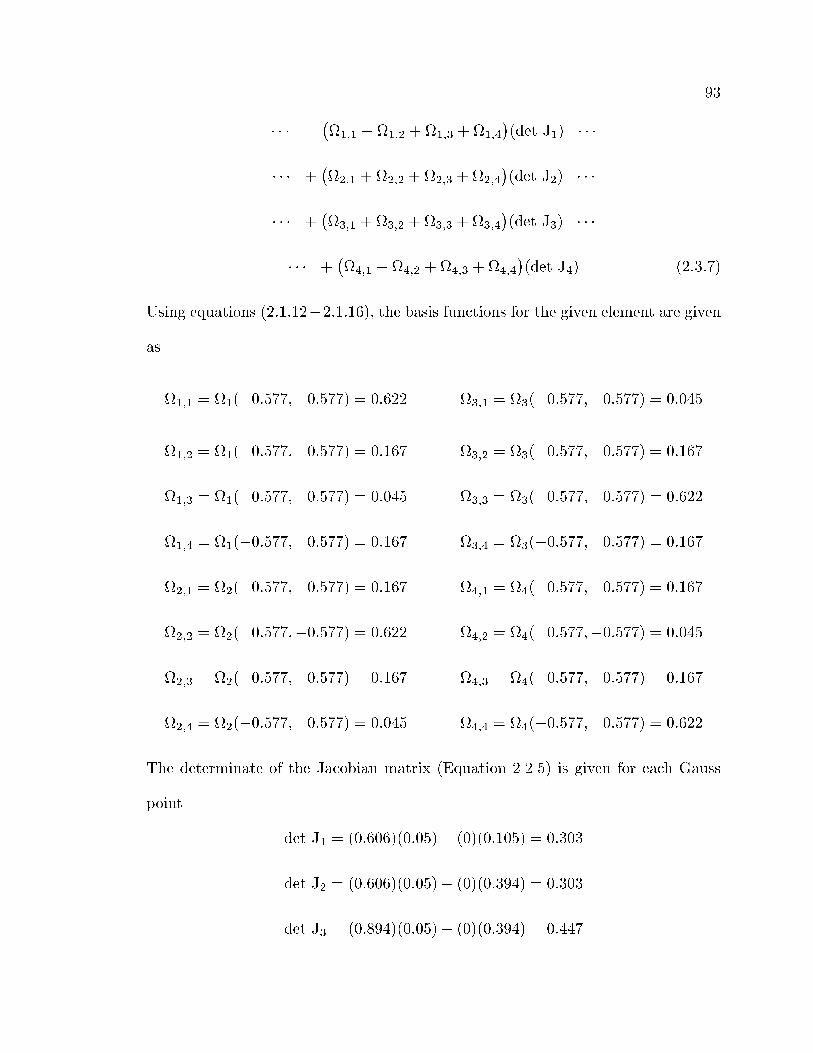
93

=1;1 + 1;2 + 1;3 + 1;4

(det J1)

+2;1 + 2;2 + 2;3 + 2;4

(det J2)

+3;1 + 3;2 + 3;3 + 3;4

(det J3)

+4;1 + 4;2 + 4;3 + 4;4

(det J4) (2:3:7)

Using equations (2:1:122:1:16), the basis functions for the given element are given

as

1;1 = 1(0:577;0:577) = 0:622 3;1 = 3(0:577;0:577) = 0:045

1;2 = 1( 0:577;0:577) = 0:167 3;2 = 3( 0:577;0:577) = 0:167

1;3 = 1( 0:577; 0:577) = 0:045 3;3 = 3( 0:577; 0:577) = 0:622

1;4 = 1(0:577; 0:577) = 0:167 3;4 = 3(0:577; 0:577) = 0:167

2;1 = 2(0:577;0:577) = 0:167 4;1 = 4(0:577;0:577) = 0:167

2;2 = 2( 0:577;0:577) = 0:622 4;2 = 4( 0:577;0:577) = 0:045

2;3 = 2( 0:577; 0:577) = 0:167 4;3 = 4( 0:577; 0:577) = 0:167

2;4 = 2(0:577; 0:577) = 0:045 4;4 = 4(0:577; 0:577) = 0:622

The determinate of the Jacobian matrix (Equation 2.2.5) is given for each Gauss

point.

det J1 = (0:606)(0:05) (0)(0:105) = 0:303

det J2 = (0:606)(0:05) (0)(0:394) = 0:303

det J3 = (0:894)(0:05) (0)(0:394) = 0:447

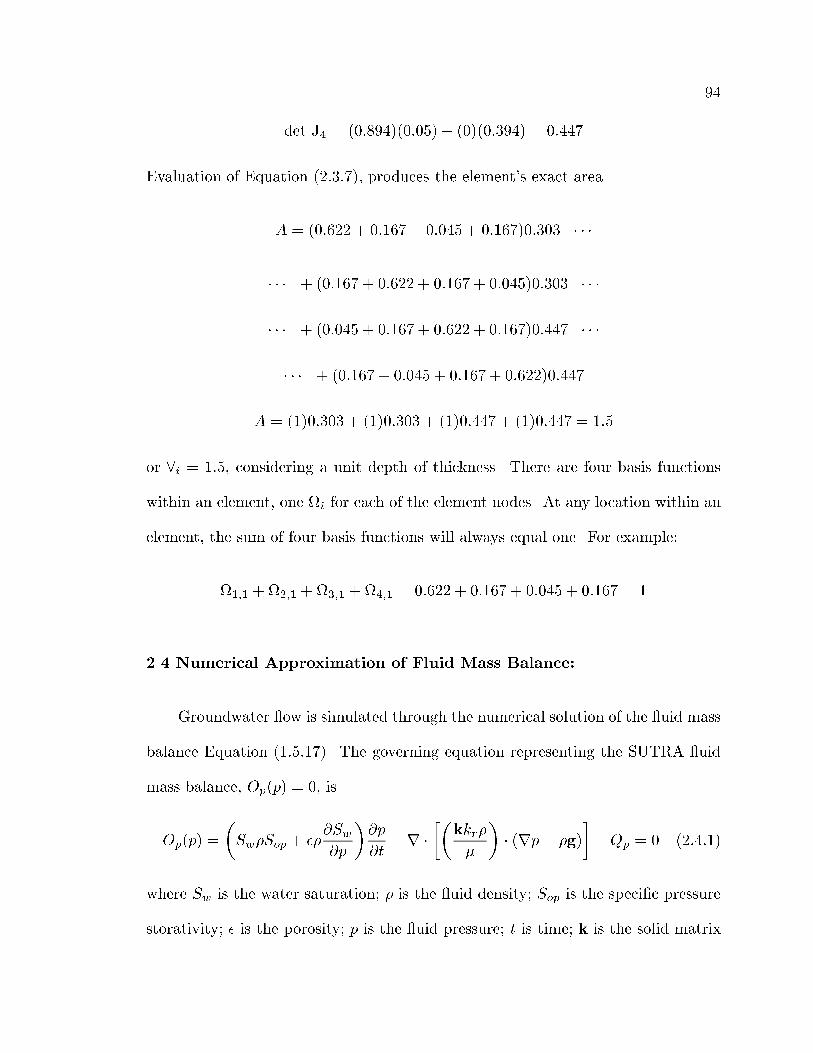
94

det J4 = (0:894)(0:05) (0)(0:394) = 0:447

Evaluation of Equation (2:3:7), produces the element's exact area.

A = (0:622 + 0:167 + 0:045 + 0:167)0:303

+ (0:167 + 0:622 + 0:167 + 0:045)0:303

+ (0:045 + 0:167 + 0:622 + 0:167)0:447

+ (0:167 + 0:045 + 0:167 + 0:622)0:447

A = (1)0:303 + (1)0:303 + (1)0:447 + (1)0:447 = 1:5

or 8i = 1:5, considering a unit depth of thickness. There are four basis functions

within an element, one i for each of the element nodes. At any location within an

element, the sum of four basis functions will always equal one. For example:

1;1 + 2;1 + 3;1 + 4;1 = 0:622 + 0:167 + 0:045 + 0:167 = 1

2.4 Numerical Approximation of Fluid Mass Balance:

Groundwater ow is simulated through the numerical solution of the uid mass

balance Equation (1:5:17). The governing equation representing the SUTRA uid

mass balance, Op(p) = 0, is

Op(p) =

SwSop +

@Sw

@p

@p

@t

r

kkr

(rp g)

Qp = 0 (2:4:1)

where Sw is the water saturation; is the uid density; Sop is the specic pressure

storativity; is the porosity; p is the uid pressure; t is time; k is the solid matrix

95

permeability; kr is the relative permeability to uid ow; is the uid viscosity; g

is the gravitational acceleration; and Qp is the uid mass source.

An additional source term is added to the mass balance Equation (2:4:1) to

account for externally specied pressure boundary conditions, pBC .

Op(p) =

SwSop +

@Sw

@p

@p

@tr

kkr

(rp g)

Qp p

pBC p

= 0 (2:4:2)

where p is the average medium conductance. Conductance is related to the cross-

sections of the elementary channels through which the ow takes place. When

conductance is set suciently large, the weight of the pressure boundary term be-

comes larger than the other terms within Equation (2:4:2). Op(p) = 0 is maintained

with an excessive source term which requires pBC = p. By forcing pBC = p, the

desired boundary condition is satised.

Spatial Integration

The uid mass balance equation, Op(p), is approximated through nodewise,

elementwise, and cellwise discretizations, Figure B.6. Spatial discretization of the

domain results in the inexact representation of variables and their derivatives. The

approximate equation, dOp(p), equals a spatially varying residual value, Rp(x; z; t),

which is no longer equal to zero.

dOp(p) = Rp(x; z; t) 6= 0 (2:4:3)

By minimizing the residual over space and time, Equation (2:4:3) is reformulated

as an optimization problem. The objective of the optimization is to determine the

96

nodal values of pi, in such a way as to minimize the residual, Rp(x; z; t). The

residual is minimized by requiring the orthogonality of the weighting functions and

the dierential. The weighted residual formulation is written as:

Z8

Rp(x; z; t)Wi(x; z)d8 =

Z8

ddOp(p)Wi(x; z)d8 = 0 i = 1;NN (2:4:4)

where Wi(x; z) is the weighting function in global coordinates; 8 is the total spatial

volume of the groundwater system; and NN is the total number of nodes within the

nite element mesh.

z

x

Figure B.6: Cells, elements and nodes for a two-dimensional finite-element mesh composed of quadrilateral elements.

CELL

ELEMENT

NODE

The Galerkin method of weighted residuals is applied, since the basis function,

i(x; z), is equal to the weighting function, Wi(x; z). Substituting i(x; z) into

97

Equation (2:4:4) yields Z8

ddOp(p)i(x; z)d8 = 0 (2:4:5)

Substitution fordd

Op(p) from Equation (2:4:2) gives,Z8

SwSop +

@Sw

@p

@p

@t

r

kkr

(rp g)

Qp p

pBC p

i(x; z)d8 = 0 (2:4:6)

or Z8

SwSop +

@Sw

@p

@p

@t

i(x; z)d8

Z8

r

kkr

(rp g)

i(x; z)d8

Z8

Qp

i(x; z)d8

Z8

p

pBC p

i(x; z)d8 = 0 (2:4:7)

The rst term in Equation (2:4:7) is an integral of the pressure derivative,Z8

" ddSwSop +

@Sw

@p

@p

@t

#i(x; z)d8

=

" ddSwSop +

@Sw

@p

@p

@t

# Z8

i(x; z)d8 (2:4:8)

where the term in brackets is discretized cellwise. From the Gaussian Integration

example, Equation (2:3:5), the integral of the basis function equals the volume of

the cell at node i. Integrating term (2:4:8) gives,SwSop +

@Sw

@p

i

@pi

@t

8i (2:4:9)

Green's Theorem is applied to the second term in Equation (2:4:7). The sym-

bolic form of Green's Theorem is given as,Z8

(r )d8 =

Z

( n)d

Z8

(r)d8 (2:4:10)

98

Application of Green's Theorem to the second term yields,

Z8

r

dkkr

(rp g)

i(x; z) d8 =

Z

" dkkr

(rp g)

# n i(x; z) d

+

Z8

" dkkr

(rp g)

# ri d8 (2:4:11)

where n is the unit vector normal to the three-dimensional surface bounding the

region to be simulated, and is the surface of the region. The basis function in

global coordinates is denoted, i(x; z). The rst term on the right of Equation

(2:4:11) is exactly the uid mass out ow, Oi(t), across the region's boundary at

node i.

Oi(t) = qA = SwvA

= Sw

"kkr

Sw

(rp g)

#A =

kkr

(rp g)A

Oi(t) =

Z

" dkkr

(rp g)

# n i(x; z) d (2:4:12)

This term is used to specify uid ows across system boundaries.

The second term on the right of Equation (2:4:11) is approximated using a

combination of elementwise and nodewise discretizations. The permeability tensor,

k, is expressed in matrix notation as,

kL =

24 kLxx

kLxy

kLxz

kLyx

kLyy

kLyz

kLzx

kLzy

kLzz

35 (2:4:13)

where the discretization of k is elementwise and is indicated by kL. A simplication

of the permeability tensor is made with the assumption of a two-dimensional model.

99

Within the third dimension, or y coordinate direction, the kxy, kyx, kyy, kyz, and

kzy components of the permeability tensor are eliminated.

kL =

kL

xxkL

xz

kL

zxkL

zz

(2:4:4)

The nite approximation of uid pressure is discretized nodewise:

p(x; z; t) =

NNXi=1

pi(t) i(x; z) (2:4:15)

where NN is the total number of nodes in the mesh. Integration of the pressure

derivative over the total spatial volume gives,

Z8

rpd8 =

NNXi=1

Z8

r

pi(t) i(x; z)

d8 =

NNXi=1

pi(t)

Z8

ri(x; z)d8 (2:4:16)

Relative permeability, kr, depends on saturation which, in turn, depends on

pressure. Relative permeabilities depend on saturation and are evaluated at each

Gauss point during numerical integration. Viscosity, , is constant throughout

space and time.

The second term on the right of Equation (2:4:11) is further developed as

follows: Z8

kLkr

rpi ri d8

Z8

kLkr

g ri d8 (2:4:17)

Substituting forRrpd8 in Equation (2:4:16) gives,

NNXi=1

pj(t)

Z8

kLkr

rj ri d8

Z8

kLkr

g ri d8

=

NNXi=1

pj(t)

Z8

(kL)

kr

rj

ri d8

100

Z8

(kL)

kr

g

ri d8 (2:4:18)

The element volume is expressed as,

d8 = dy dz dx = B(x; z)dzdx (2:4:19)

where B(x; z) is the thickness of the mesh within the y-coordinate direction. The

thickness is assumed equal to one throughout space and time. Substitution for d8,

in Equation (2:4:18), gives

NNXi=1

pj(t)

Z8

(kL)

kr

rj

riB(x; z)dzdx

Z8

(kL)

kr

g

riB(x; z)dzdx (2:4:20)

where (kr) is a term based on nodewise discretized values of pressure, p.

The last two terms of Equation (2:4:6) are approximated cellwise. Both the

uid mass source term, Qp, and conductance, p, are averaged over the volume of

a cell i.

Qp =

NNXi=1

Qi

8i

(2:4:21)

p =

NNXi=1

i

8i

(2:4:22)

A single cell representation, with substitutions made for Qp and p, gives the last

two terms of Equation (2:4:7) as,

Z8

Qi

8i

i(x; z)d8

Z8

i

8i

(pBCi

pi)

i(x; z)d8

=

Qi

8i

Z8

i(x; z)d8

i

8i

(pBCi

pi)

Z8

i(x; z)d8

101

=

Qi

8i

8i

i

8i

(pBCi

pi)

8i

= Qi i(pBCi pi) (2:4:23)

By combining and rearranging the evaluations of approximate terms of Equa-

tion (2:4:7), the following weighted residual relation is obtained:

AFidpi

dt BFi +

NNXj=1

pj(t)CFij DFi Qi

i(pBCi

pi)= 0

i = 1;NN (2:4:24)

or

AFidp

dti+

NNXj=1

pj(t)CFij + ipi = Qi + ipBCi+ BFi + DFi

i = 1;NN (2:4:25)

where:

AFi =

SwSop +

@Sw

@p

i

8i

BFi =

Z

"kkr

(rp g)

# n i d

CFij =

Zx

Zz

kL

kr

rj

ri Bdzdx

DFi =

Zx

Zz

kL

kr

[g]

rj Bdzdx

The integrals requiring Gaussian integration are BFi, CFij , and DFi. The other

terms, except for those involving i, are evaluated cellwise.

102

Temporal Discretization

The time derivatives in the spatially discretized and integrated equation are

approximated by nite dierences. The pressure term is approximated as,

dpi

dt=

pn+1i

pni

tn+1(2:4:26)

where

pni= pi(t

n)

pn+1i

= pi(tn +tn+1) = pi(t

n+1)

tn+1 = tn+1 tn

The current time step, tn+1, begins at time tn and ends at time tn+1. The

previous time step for which a solution has already been obtained at time tn is

denoted tn. Temporal denitions are given in Figure B.7, where p0 is the initial

pressure distribution at t0 = 0 seconds.

t

tn-1t0 tn

p0 pn-1 pn pn+1

tn+1

∆tn+1∆tn

Figure B.7: Temporal definitions.

All other terms in Equation (2:4:25) are evaluated at the new time tn+1 for

the solution of the present time step, tn+1. For each time step, coecients are

103

based on a projected value of uid pressure, p. The projected pressure, pproj

i , is

an estimation of p at the end of the present time step, tn+1, based on the linear

extrapolation of the two previous values of p. The projected pressure is determined

with a linear extrapolation between (tn1; pn1) and (tn; pn).

pi pni =

pni p

n1i

tn1 tn

[t t

n] =

pni p

n1i

tn

[t t

n]

pi =

pni p

n1i

tn

[t t

n] + pni (2:4:27)

At tn+1 the projected pressure, p

proj

i , is given as

pproj

i =

pni p

n1i

tn

[tn+1 t

n] + pni =

pni p

n1i

tn

tn+1 + p

ni

= pni +

tn+1

tn

pni p

n1i

(2:4:28)

The weighted residual relation, Equation (2:4:25), is then written in a form

which allows for the solution of pressures at nodes, pn+1i , at the end of the present

time step,

AFn+1i

pn+1i p

ni

tn+1

+

NNXj=1

pn+1j (t)CFn+1ij + ip

n+1i

= Qn+1i + ip

n+1BCi

+ BFn+1i +DF(n+1)

i i = 1;NN (2:4:29)

or AFn+1i

tn+1

pn+1i +

NNXj=1

pn+1j (t)CFn+1ij + ip

n+1i

= Qn+1i + ip

n+1BCi

+ BFn+1i +DF(n+1)

i +

AFn+1i

tn+1

pni i = 1;NN (2:4:30)

where the superscript involving (n) or (n+ 1) indicates the time of evaluation.

APPENDIX C: Scenario 1 Sensitivity

Pressure RMSE = Root Mean Squared Error = SQRTSUM[(p_base - p)^2]/NNCOMP TIME = Computational time required to complete a given simulation.

RATE OF CHANGE = Mass budget, rate of change in total stored fluid due to pressure change [kg/m].Net Inflow (+) / Net outflow (-)

TOTAL OF FLOWS = Mass budget, total of fluid flows at points of specified pressure [kg/m].Net Inflow (+) / Net outflow (-)

Base = Base case value.

INTRINSIC PERMEABILITYPRESSURE SATURATION ANGLE MAGNITUDE COMP TIME RATE OF TOTAL OF

PERM RMSE RMSE RMSE RMSE (min) CHANGE FLOWS1.E-13 17842 0.509 63.7 7.74E-05 25.7 -0.001 -0.0011.E-12 16783 0.489 62.5 6.73E-05 25.6 -0.010 -0.0105.E-12 10198 0.353 56.6 3.95E-05 25.8 -0.048 -0.049

Base 1.E-11 0 0.000 0.0 0.00E+00 26.1 -0.058 -0.0625.E-11 7057 0.352 46.9 7.86E-05 26.9 0.000 0.0001.E-10 7053 0.355 52.5 7.86E-05 27.0 0.000 0.000

POROSITYPRESSURE SATURATION ANGLE MAGNITUDE COMP TIME RATE OF TOTAL OF

POR RMSE RMSE RMSE RMSE (min) CHANGE FLOWS0.01 4249 0.25 52.0 4.1E-04 26.18 -0.029 -0.0290.05 2224 0.18 47.0 6.0E-05 26.14 -0.077 -0.047

Base 0.10 0 0.00 0.0 0.0E+00 26.07 -0.058 -0.0620.15 2275 0.18 46.8 2.7E-05 26.02 -0.086 -0.0760.20 4266 0.24 50.4 3.8E-05 26.08 -0.106 -0.0840.25 5465 0.26 49.6 4.4E-05 26.15 -0.081 -0.0870.30 7627 0.31 54.2 4.8E-05 25.90 -0.091 -0.091

TEMPORAL STEP SIZEPRESSURE SATURATION ANGLE MAGNITUDE COMP TIME RATE OF TOTAL OF

DT RMSE RMSE RMSE RMSE (min) CHANGE FLOWS2 3228 0.206 51.9 3.7E-05 129.8 -0.078 -0.0795 1318 0.126 48.1 2.0E-05 52.1 -0.031 -0.070

Base 10 0 0.000 0.0 0.0E+00 26.1 -0.058 -0.06220 854 0.110 41.7 1.5E-05 13.1 -0.085 -0.05740 1041 0.121 42.1 1.7E-05 6.7 -0.061 -0.054

100 877 0.118 42.8 1.3E-05 2.7 -0.052 -0.057200 879 0.107 38.6 8.5E-06 1.4 -0.101 -0.059500 2086 0.147 47.5 1.9E-04 0.6 -0.093 -0.065

PARTIALLY SATURATED PARAMETERSPRESSURE SATURATION ANGLE MAGNITUDE COMP TIME RATE OF TOTAL OF

Soil Type RMSE RMSE RMSE RMSE (min) CHANGE FLOWSSandy loam 3547 0.272 58.0 4.2E-05 26.47 -0.033 -0.036

Silt loam 586 0.077 39.4 1.3E-05 26.18 -0.052 -0.067Loam 483 0.070 38.8 9.2E-06 26.25 -0.250 -0.066

Base Sandy clay loam 0 0.000 0.0 0.0E+00 26.07 -0.058 -0.062Silty clay loam 2199 0.175 47.9 2.9E-05 26.23 -0.072 -0.074

Clay loam 3048 0.218 50.9 3.9E-05 26.17 -0.046 -0.039Beit Netofa Clay 3847 0.233 46.9 4.2E-05 25.96 -0.080 -0.081

a [1/m] n Ssat Swres

Sandy loam 2.77 2.89 0.44 0.00 (Shao and Horton, 1998)Silt loam 10.92 1.18 0.50 0.00 (Shao and Horton, 1998)

Loam 17.81 1.16 0.50 0.00 (Shao and Horton, 1998)Sandy clay loam 0.58 1.59 0.54 0.09 (Shao and Horton, 1998)

Silty clay loam 1.36 1.24 0.56 0.00 (Shao and Horton, 1998)Clay loam 1.25 2.38 0.56 0.07 (Shao and Horton, 1998)

Beit Netofa Clay 0.152 1.17 0.446 0.00 (van Genuchten, 1980)

104

Total Number of Elements 105Num. of PRESSURE SATURATION COMP TIME RATE OF TOTAL OF Position X Position ZElements RMSE RMSE (min) CHANGE FLOWS 2.5126 96.6291

7157 1475 0.043 186.7 -0.066 -0.066 11.102 98.85224186 966 0.010 63.6 -0.099 -0.063 16.6289 101.839

Base 2696 0 0.000 33.7 -0.079 -0.065 25.4377 101.7281877 1127 0.040 34.3 -0.061 -0.064 34.0224 105.7911404 1552 0.012 9.1 -0.058 -0.063 46.9804 111.61

Note: The RMSE analysis was conducted with the following 51.6938 115.052nodal positions (X, Z). 57.176 112.97

64.0599 113.4568.2611 11697879.0315 112.309

106

APPENDIX D: Sample SUTRA.d55 Input File SUTRA SOLUTE TRANSPORT SUTRA Model created using ArgusONE E-Road System Scenario 3 4183 3949 93 0 242 0 234 0 6 308 1 0 0 -1 1317 0. 0.01 1. 99999 200. 5270400. 9999 1. 200. 1 1 1317 1 0 0 0 0 1 1 1 0. 0. 2.718e-06 1. 1.e-09 1000. 0. 700. 0.001 1.27e-06 0. 0. 1025. NONE 0. 0. 0. 0. 0. 0. 0. -9.81 NODE 1 1 1 1 1 0 87.333 127.28566 1. 0.1 2 0 87.054163 127.19016 1. 0.1 3 0 87.333 126.80432 1. 0.1 4 0 86.936639 126.86404 1. 0.1 5 0 87.333 127.52633 1. 0.1 6 0 87.109383 127.43238 1. 0.1 7 0 86.843822 127.25948 1. 0.1 8 0 86.954185 127.62555 1. 0.1 9 0 86.58868 127.02331 1. 0.1 10 0 87.06702 126.54291 1. 0.1 **** * ********* ********* * *** **** * ********* ********* * *** **** * ********* ********* * *** 4175 0 0.867 96.633 1. 0.1 4176 0 1.1565557 95.164978 1. 0.1 4177 0 0.867 95.333 1. 0.1 4178 0 1.2168073 95.020472 1. 0.1 4179 0 1.2566953 94.853684 1. 0.1 4180 0 1.110322 94.902296 1. 0.1 4181 0 0.867 95.033 1. 0.1 4182 0 0.867 94.883 1. 0.1 4183 0 0.867 94.733 1. 0.1 ELEMENT 1 1 1 1 1 1 1 1 0 1.e-11 1.e-11 0. 0.5 0.5 0.1 0.1 2 0 1.e-11 1.e-11 0. 0.5 0.5 0.1 0.1 3 0 6.e-13 6.e-13 0. 0.5 0.5 0.1 0.1 4 0 1.e-11 1.e-11 0. 0.5 0.5 0.1 0.1 5 0 7.e-14 7.e-14 0. 0.5 0.5 0.1 0.1 6 0 7.e-14 7.e-14 0. 0.5 0.5 0.1 0.1 7 0 7.e-14 7.e-14 0. 0.5 0.5 0.1 0.1 8 0 7.e-14 7.e-14 0. 0.5 0.5 0.1 0.1 9 0 7.e-14 7.e-14 0. 0.5 0.5 0.1 0.1 10 0 7.e-14 7.e-14 0. 0.5 0.5 0.1 0.1 **** * ****** ****** * *** *** *** *** **** * ****** ****** * *** *** *** *** **** * ****** ****** * *** *** *** *** 3940 0 6.e-13 6.e-13 0. 0.5 0.5 0.1 0.1 3941 0 6.e-13 6.e-13 0. 0.5 0.5 0.1 0.1 3942 0 6.e-13 6.e-13 0. 0.5 0.5 0.1 0.1 3943 0 6.e-13 6.e-13 0. 0.5 0.5 0.1 0.1 3944 0 6.e-13 6.e-13 0. 0.5 0.5 0.1 0.1 3945 0 6.e-13 6.e-13 0. 0.5 0.5 0.1 0.1 3946 0 1.e-11 1.e-11 0. 0.5 0.5 0.1 0.1 3947 0 7.e-14 7.e-14 0. 0.5 0.5 0.1 0.1 3948 0 3.e-13 3.e-13 0. 0.5 0.5 0.1 0.1 3949 0 3.e-13 3.e-13 0. 0.5 0.5 0.1 0.1 -8 0. 0. -15 0. 0. -16 0. 0. -18 0. 0.

107 -27 0. 0. -38 0. 0. -51 0. 0. -66 0. 0. -83 0. 0. -100 0. 0. ***** * ** ***** * ** ***** * ** -4104 0. 0. -4112 0. 0. -4119 0. 0. -4126 0. 0. -4135 0. 0. -4143 0. 0. -4149 0. 0. -4164 0. 0. -4165 0. 0. -4175 0. 0. 00000000000000000000000000000000000000000000000000000000000000000000000000000017 -8 -80. 0. -15 -80. 0. -16 -80. 0. -18 -80. 0. -27 -80. 0. -38 -80. 0. -51 -80. 0. -66 -80. 0. -83 -80. 0. -100 -80. 0. ***** *** ** ***** *** ** ***** *** ** -4165 -80. 0. 4171 3641.6333523700741 0. 4172 6678.7555682467064 0. 4173 1820.8166761849675 0. 4174 9715.8777841233386 0. -4175 -80. 0. 4177 12752.999999999973 0. 4181 15695.999999999944 0. 4182 17167.499999999862 0. 4183 18638.999999999916 0. 00000000000000000000000000000000000000000000000000000000000000000000000000000019 86 1437 2009 2779 3267 3557 3739 0 1 6 5 15 8 2 4157 4171 4172 4159 3 4170 4174 4177 4168 4 4170 4159 4172 4174 5 4166 4168 4177 4176 6 4154 4155 4145 4144 7 4154 4166 4167 4155 8 4137 4138 4129 4128 9 4137 4144 4145 4138 10 4121 4122 4115 4114 **** **** **** **** **** **** **** **** **** **** **** **** **** **** **** 3940 608 611 609 591 3941 610 609 611 626 3942 1561 1530 1527 1559 3943 914 941 915 913 3944 1165 1167 1171 1181 3945 1150 1171 1167 1144 3946 4161 4146 4150 4163 3947 4178 4176 4177 4181 3948 2966 3005 3007 2971 3949 3008 3007 3005 3004

simula tion of p ar tiall y sa tura ted - fs.fed.us tion of p ar tiall y sa tura ted-flo w in the...

Documents