simulation-based building energy...
TRANSCRIPT

Simulation-Based Building Energy Optimization
by
Michael Wetter
A dissertation submitted in partial satisfaction of therequirements for the degree of
Doctor of Philosophy
in
Engineering — Mechanical Engineering
in the
GRADUATE DIVISIONof the
UNIVERSITY OF CALIFORNIA, BERKELEY
Committee in charge:
Prof. Elijah Polak, Co-chairProf. Van P. Carey, Co-chair
Prof. Alice M. AgoginoProf. Alexandre J. Chorin
Spring 2004

The dissertation of Michael Wetter is approved:
Co-chair Date
Co-chair Date
Date
Date
University of California, Berkeley
Spring 2004

Simulation-Based Building Energy Optimization
Copyright 2004
by
Michael Wetter

1
Abstract
Simulation-Based Building Energy Optimization
by
Michael Wetter
Doctor of Philosophy in Engineering — Mechanical Engineering
University of California, Berkeley
Prof. Elijah Polak, Co-chair
Prof. Van P. Carey, Co-chair
This dissertation presents computational techniques for simulation-based design opti-
mization of buildings and heating, ventilation, air-conditioning and lighting systems in
which the cost function is smooth. In such problems, the evaluation of the cost function
involves the numerical solution of systems of differential algebraic equations (DAE).
Since the termination criteria of the iterative solvers often depend on the design param-
eters, a computer code for solving such systems usually defines a numerical approxima-
tion to the cost function that is discontinuous in the design parameters. The disconti-
nuities can be large in cost functions that are evaluated by commercial building energy
simulation programs, and optimization algorithms that require smoothness frequently
fail if used with such programs. Furthermore, controlling the numerical approximation

2
error is often not possible with commercial building energy simulation programs.
In this dissertation, we present BuildOpt, a new detailed thermal building and day-
lighting simulation program. BuildOpt’s simulation models define a DAE system that is
smooth in the state variables, in time and in the design parameters. This allows proving
that the DAE system has a unique solution that is smooth in the design parameters, and
it is required to compute high precision approximating cost functions that converge to
a cost function that is smooth in the design parameters as the DAE solver tolerance is
tightened.
For simulation programs that allow such a precision control, we constructed subpro-
cedures for Generalized Pattern Search (GPS) optimization algorithms that adaptively
control the precision of the cost function evaluations: coarse precision for the early iter-
ations, with precision progressively increasing as a stationary point is approached. This
scheme significantly reduces the computation time, and it allows to prove that the se-
quence of iterates contains stationary accumulation points.
For optimization problems in which commercial building energy simulation pro-
grams are used to evaluate the cost function, we compared by numerical experiment
several deterministic and probabilistic optimization algorithms.
Co-chair Date
Co-chair Date

i
To Maureen.
To my parents.

ii
Contents
List of Figures v
List of Tables viii
Conventions and Symbols ix
Acknowledgements xiii
1 Introduction 11.1 Problem Discussion . . . . . . . . . . . . . . . . . . . . . . . . . . . . 2
1.1.1 Optimization Problem . . . . . . . . . . . . . . . . . . . . . . 21.1.2 Approximating Optimization Problems . . . . . . . . . . . . . 41.1.3 Commercial Building Energy Simulation Programs . . . . . . . 5
1.2 Objective of the Dissertation . . . . . . . . . . . . . . . . . . . . . . . 61.3 Market for Building and HVAC Design Optimization . . . . . . . . . . 71.4 Review of State-of-the-Art . . . . . . . . . . . . . . . . . . . . . . . . 8
1.4.1 Building Energy Simulation Programs . . . . . . . . . . . . . . 81.4.2 Optimization with Adaptive Precision Cost Function Evaluations 101.4.3 Optimization with Fixed Precision Cost Function Evaluations . 111.4.4 Building and HVAC Design Optimization . . . . . . . . . . . . 14
1.5 Proposed New Approach . . . . . . . . . . . . . . . . . . . . . . . . . 151.5.1 Optimization with Adaptive Precision Cost Function Evaluations 161.5.2 Optimization with Fixed Precision Cost Function Evaluations . 20
2 BuildOpt – A Building Simulation Program Built on Smooth Models 222.1 Introduction . . . . . . . . . . . . . . . . . . . . . . . . . . . . . . . . 232.2 Properties of Optimization Problem . . . . . . . . . . . . . . . . . . . 26
2.2.1 Statement of the Optimization Problem . . . . . . . . . . . . . 262.2.2 Existence of a Unique Smooth Solution of the DAE System . . 282.2.3 Numerical Solutions of the DAE System . . . . . . . . . . . . 30

iii
2.2.4 Mathematical Requirements on the Solutions of the DAE System 302.3 BuildOpt Simulation Program . . . . . . . . . . . . . . . . . . . . . . 32
2.3.1 Simulation Model Generator . . . . . . . . . . . . . . . . . . . 332.3.2 Smoothing Techniques . . . . . . . . . . . . . . . . . . . . . . 342.3.3 Solving the Equations . . . . . . . . . . . . . . . . . . . . . . 362.3.4 Model Validation . . . . . . . . . . . . . . . . . . . . . . . . . 37
2.4 Numerical Experiments . . . . . . . . . . . . . . . . . . . . . . . . . . 372.5 Conclusion . . . . . . . . . . . . . . . . . . . . . . . . . . . . . . . . 42
3 Optimization with Adaptive Precision Cost Function Evalutions 433.1 Introduction . . . . . . . . . . . . . . . . . . . . . . . . . . . . . . . . 443.2 Optimization Problem . . . . . . . . . . . . . . . . . . . . . . . . . . . 473.3 Precision Control for Generalized Pattern Search Algorithms . . . . . . 50
3.3.1 Characterization of Generalized Pattern Search Algorithms . . . 503.3.2 Adaptive Precision GPS Algorithm Models . . . . . . . . . . . 53
3.4 Convergence Analysis . . . . . . . . . . . . . . . . . . . . . . . . . . 583.4.1 Unconstrained Minimization . . . . . . . . . . . . . . . . . . . 583.4.2 Constrained Minimization . . . . . . . . . . . . . . . . . . . . 63
3.5 Numerical Experiments . . . . . . . . . . . . . . . . . . . . . . . . . . 663.5.1 Cost Function defined on the Solutions of a DAE System . . . . 673.5.2 Cost Function defined on the Solutions of a Nonlinear Equations 76
3.6 Conclusion . . . . . . . . . . . . . . . . . . . . . . . . . . . . . . . . 82
4 Optimization with Fixed Precision Cost Function Evaluations 844.1 Introduction . . . . . . . . . . . . . . . . . . . . . . . . . . . . . . . . 854.2 Optimization Problem . . . . . . . . . . . . . . . . . . . . . . . . . . . 884.3 Simulation Models . . . . . . . . . . . . . . . . . . . . . . . . . . . . 91
4.3.1 Simple Simulation Model . . . . . . . . . . . . . . . . . . . . 924.3.2 Detailed Simulation Model . . . . . . . . . . . . . . . . . . . . 94
4.4 Optimization Algorithms . . . . . . . . . . . . . . . . . . . . . . . . . 964.4.1 Coordinate Search Algorithm . . . . . . . . . . . . . . . . . . 964.4.2 Hooke-Jeeves Algorithm . . . . . . . . . . . . . . . . . . . . . 974.4.3 Particle Swarm Optimization Algorithms . . . . . . . . . . . . 984.4.4 Particle Swarm Optimization Algorithm that Searches on a Mesh 994.4.5 Hybrid Particle Swarm and Hooke-Jeeves Algorithm . . . . . . 1004.4.6 Simple Genetic Algorithm . . . . . . . . . . . . . . . . . . . . 1014.4.7 Simplex Algorithm of Nelder and Mead . . . . . . . . . . . . . 1024.4.8 Discrete Armijo Gradient Algorithm . . . . . . . . . . . . . . . 103
4.5 Numerical Experiments . . . . . . . . . . . . . . . . . . . . . . . . . . 1044.5.1 Comparison of the Optimization Results . . . . . . . . . . . . . 1044.5.2 Discontinuities in the Cost Function . . . . . . . . . . . . . . . 110

iv
4.6 Conclusion . . . . . . . . . . . . . . . . . . . . . . . . . . . . . . . . 114
Bibliography 130
A BuildOpt – Model Description 131A.1 Introduction . . . . . . . . . . . . . . . . . . . . . . . . . . . . . . . . 132
A.1.1 Objective and Scope of the Simulation Program . . . . . . . . . 132A.1.2 Model Description . . . . . . . . . . . . . . . . . . . . . . . . 133
A.2 Conventions . . . . . . . . . . . . . . . . . . . . . . . . . . . . . . . . 135A.3 Approximations for Non-Differentiable Functions . . . . . . . . . . . . 136
A.3.1 Approximation for P-Controller . . . . . . . . . . . . . . . . . 136A.3.2 Approximation for Heaviside Function . . . . . . . . . . . . . 138A.3.3 Approximation for Minimum and Maximum Function . . . . . 139
A.4 Physical Model . . . . . . . . . . . . . . . . . . . . . . . . . . . . . . 140A.4.1 Introduction . . . . . . . . . . . . . . . . . . . . . . . . . . . . 140A.4.2 External and Internal Heat Gains . . . . . . . . . . . . . . . . . 140A.4.3 Heat Transfer in the Building . . . . . . . . . . . . . . . . . . . 169A.4.4 Daylighting and Electric Lighting . . . . . . . . . . . . . . . . 245
A.5 Implementation of the Models and the DAE Solver . . . . . . . . . . . 266A.6 Compiling and Linking BuildOpt . . . . . . . . . . . . . . . . . . . . . 267
B BuildOpt – Validation 268B.1 Thermal Model . . . . . . . . . . . . . . . . . . . . . . . . . . . . . . 269
B.1.1 Introduction . . . . . . . . . . . . . . . . . . . . . . . . . . . . 269B.1.2 Specification of the Test Cases . . . . . . . . . . . . . . . . . . 269B.1.3 Modeling Notes . . . . . . . . . . . . . . . . . . . . . . . . . . 274B.1.4 Results . . . . . . . . . . . . . . . . . . . . . . . . . . . . . . 279B.1.5 Conclusions . . . . . . . . . . . . . . . . . . . . . . . . . . . . 298
B.2 Daylighting Model . . . . . . . . . . . . . . . . . . . . . . . . . . . . 299B.2.1 Introduction . . . . . . . . . . . . . . . . . . . . . . . . . . . . 299B.2.2 Specification of the Test Cases . . . . . . . . . . . . . . . . . . 300B.2.3 Results . . . . . . . . . . . . . . . . . . . . . . . . . . . . . . 303B.2.4 Conclusions . . . . . . . . . . . . . . . . . . . . . . . . . . . . 309

v
List of Figures
1.1 Computation time as a function of the DAE solver tolerance. . . . . . . 171.2 Diagonalization scheme. . . . . . . . . . . . . . . . . . . . . . . . . . 181.3 Approach for developing a fast convergent optimization technique. . . . 19
2.1 Convergence of approximating cost functions to a smooth function. . . 41
3.1 Thermal zones used for computing the energy consumption. . . . . . . 673.2 Convergence to a minimum. . . . . . . . . . . . . . . . . . . . . . . . 753.3 Convergence to a minimum. . . . . . . . . . . . . . . . . . . . . . . . 81
4.1 Buildings used in the numerical experiments. . . . . . . . . . . . . . . 924.2 Number of simulations vs. distance to lowest cost. . . . . . . . . . . . . 1094.3 Discontinuities in approximating cost function. . . . . . . . . . . . . . 1114.4 Discontinuities in approximating cost function. . . . . . . . . . . . . . 112
A.1 Approximation to P-controller. . . . . . . . . . . . . . . . . . . . . . . 138A.2 Declination δ, latitude λ and solar hour ω. . . . . . . . . . . . . . . . . 143A.3 Solar zenith angle and azimuth. . . . . . . . . . . . . . . . . . . . . . . 144A.4 Coordinate system used to obtain the solar incidence angle. . . . . . . . 144A.5 Solar incidence angle on a tilted surface. . . . . . . . . . . . . . . . . . 146A.6 Approximate solution constructed by the Galerkin method. . . . . . . . 180A.7 Master element with master basis functions. . . . . . . . . . . . . . . . 182A.8 Transmittance and absorbtance of a window. . . . . . . . . . . . . . . . 189A.9 Infinite long window overhang. . . . . . . . . . . . . . . . . . . . . . . 221A.10 Nomenclature for heat balance of a window . . . . . . . . . . . . . . . 226A.11 Conductivity of window gap. . . . . . . . . . . . . . . . . . . . . . . . 230A.12 Location of patches for daylighting model. . . . . . . . . . . . . . . . . 245A.13 Nomenclature for view factor calculation. . . . . . . . . . . . . . . . . 248A.14 Altitude and azimuth angle of the window edges . . . . . . . . . . . . . 250A.15 Nomenclature used in computing fdAp,gro(z;x). . . . . . . . . . . . . . 254

vi
A.16 Spherical distribution of the diffuse illuminance. . . . . . . . . . . . . . 255A.17 Nomenclature used for computing the diffuse illuminance on ∆Ap. . . . 256A.18 Location of elements used for approximating the window transmittance. 257A.19 Power/light curve for continuous dimming. . . . . . . . . . . . . . . . 261
B.1 Isometric view of building with south windows. . . . . . . . . . . . . . 271B.2 Isometric view of building with west and east windows. . . . . . . . . . 271B.3 Isometric view of building with sunspace. . . . . . . . . . . . . . . . . 272B.4 Annual heating loads for low mass buildings. . . . . . . . . . . . . . . 279B.5 Annual sensible cooling loads for low mass buildings. . . . . . . . . . . 280B.6 Peak heating loads for low mass buildings. . . . . . . . . . . . . . . . . 280B.7 Annual peak sensible cooling loads for low mass buildings. . . . . . . . 281B.8 Annual heating loads for high mass buildings. . . . . . . . . . . . . . . 281B.9 Annual sensible cooling loads for high mass buildings. . . . . . . . . . 282B.10 Peak heating loads for high mass buildings. . . . . . . . . . . . . . . . 282B.11 Annual peak sensible cooling loads for high mass buildings. . . . . . . 283B.12 Sensitivity of annual heating load for low mass buildings. . . . . . . . . 283B.13 Sensitivity of annual sensible cooling load for low mass buildings. . . . 284B.14 Sensitivity of peak heating load for low mass buildings. . . . . . . . . . 284B.15 Sensitivity of peak sensible cooling load for low mass buildings. . . . . 285B.16 Sensitivity of annual heating load for high mass buildings. . . . . . . . 285B.17 Sensitivity of annual sensible cooling load for high mass buildings. . . . 286B.18 Sensitivity of peak heating load for high mass buildings. . . . . . . . . 286B.19 Sensitivity of peak sensible cooling load for high mass buildings. . . . . 287B.20 Minimum hourly annual temperature for free-float test cases. . . . . . . 289B.21 Average hourly annual temperature for free-float test cases. . . . . . . . 289B.22 Maximum hourly annual temperature for free-float test cases. . . . . . . 290B.23 Annual hourly temperature frequency for each 1C bin. . . . . . . . . . 291B.24 Hourly free float temperatures on January 4 for low mass building. . . . 291B.25 Hourly free float temperatures on January 4 for heavy mass building. . . 292B.26 Annual incident solar radiation. . . . . . . . . . . . . . . . . . . . . . . 293B.27 Annual transmitted solar radiation with unshaded windows. . . . . . . . 294B.28 Annual transmitted solar radiation with shaded windows. . . . . . . . . 294B.29 Hourly incident solar radiation on a cloudy day (south). . . . . . . . . . 295B.30 Hourly incident solar radiation on a clear day (south). . . . . . . . . . . 295B.31 Hourly incident solar radiation on a cloudy day (west). . . . . . . . . . 296B.32 Hourly incident solar radiation on a clear day (west). . . . . . . . . . . 296B.33 Annual transmissivity coefficient of windows. . . . . . . . . . . . . . . 297B.34 Annual overhang and fin shading coefficients. . . . . . . . . . . . . . . 297B.35 Hourly heating and cooling power on January 4 for low mass building. . 298B.36 LESO scale model. . . . . . . . . . . . . . . . . . . . . . . . . . . . . 300

vii
B.37 CSTB scale model. . . . . . . . . . . . . . . . . . . . . . . . . . . . . 302B.38 Daylight factors for the LESO scale model. . . . . . . . . . . . . . . . 305B.39 Daylight factors for the CSTB/ECAD scale model with an isotropic sky. 307

viii
List of Tables
2.1 Effect of smoothing methods on computation times. . . . . . . . . . . . 40
3.1 Normalized computation times for the optimization. . . . . . . . . . . . 723.2 Normalized computation times for the optimization. . . . . . . . . . . . 80
4.1 Overview of design variables and attained cost reduction. . . . . . . . . 944.2 Comparison of the optimization algorithm performances. . . . . . . . . 106
A.1 Perez model coefficients for irradiance. . . . . . . . . . . . . . . . . . 155A.2 Coefficients for angular dependency of window properties. . . . . . . . 195
B.1 Description of base cases. . . . . . . . . . . . . . . . . . . . . . . . . . 273B.2 Reflectance values for the LESO scale model. . . . . . . . . . . . . . . 301B.3 Reflectance values for the CSTB scale model. . . . . . . . . . . . . . . 301B.4 Daylight factors for the LESO scale model. . . . . . . . . . . . . . . . 304B.5 Daylight factors for the CSTB/ECAD scale model. . . . . . . . . . . . 308

ix
Conventions and Symbols
Numbering and Cross-Referencing System
The following system of numbering and cross-referencing is used.
Definitions, assumptions, lemmas, propositions, theorems, corollaries and remarks
are numbered in order of occurrence and using a three number system (a.b.c), where a is
the chapter number, b is the section number, and c is the item number. This numbering
system does not distinguish between definitions, assumptions, lemmas, etc.
Within each section, equations are numbered consecutively, using a single number
system, and are referred to by a three number system (a.b.c), where a is the chapter
number, b is the section number, and c is the item number.
Conventions
1. Rn denotes the Euclidean space of n-tuplets of real numbers. Vectors x ∈ Rn are
always column vectors, and their elements are denoted by superscripts. The inner
product in Rn is denoted by 〈·, ·〉 and for x,y∈Rn it is defined by 〈x,y〉, ∑ni=1 xi yi.
The norm in Rn is denoted by ‖ · ‖ and for x ∈ Rn defined by ‖x‖, 〈x,x〉1/2.
2. We denote by Z the set of integers, by Q the set of rational numbers, and by N ,
0, 1, . . . the set of natural numbers. The set N+ is defined as N+ , 1, 2, . . ..

x
Similarly, vectors in Rn with strictly positive elements are denoted by Rn+ , x ∈
Rn | xi > 0, i ∈ 1, . . . ,n and the set Q+ is defined as Q+ , q ∈Q | q > 0.
3. For ε ∈ Rq+, by ε≤ εS, we mean that 0 < εi ≤ εi
S, for all i ∈ 1, ... ,q.
4. f (·) denotes a function where (·) stands for the undesignated variables. f (x) de-
notes the value of f (·) for the argument x. f : A→ B indicates that the domain of
f (·) is in the space A, and that the image of f (·) is in the space B.
5. We say that a function f : Rn → Rm is Lipschitz continuous on a set S ⊂ Rn,
with respect to (w.r.t.) x ∈ S, if f (·) is defined on S, and if there exists a constant
L ∈ (0,∞) such that ‖ f (x′)− f (x′′)‖ ≤ L‖x′− x′′‖, for all x′,x′′ ∈ S.
6. We say that a function f : Rn→ R is k-times (Lipschitz) continuously differen-
tiable on a set S⊂ Rn, with respect to (w.r.t.) x ∈ S, if f (·) is defined on S, and if
f (·) has k (Lipschitz) continuous derivatives on S.
7. If a subsequence xii∈K ⊂ xi∞i=0 converges to some point x, we write xi→K x.
8. Let W be a set containing a sequence wiki=0. Then, we denote by wk the sequence
wiki=0 and by Wk the set of all k +1 element sequences in W.
9. We denote by eini=1 the unit vectors in Rn.
10. If X is a set, we denote by ∂X its boundary.
11. If S is a set, we denote by 2S the set of all nonempty subsets of S.
xi
12. If D ∈ Qn×q is a matrix, we will use the notation d ∈ D to denote the fact that
d ∈Qn is a column vector of the matrix D.
13. For s ∈ R, we define bsc, maxk ∈ Z | k ≤ s and dse, mink ∈ Z | k ≥ s.
14. We denote by H : R→ R the Heaviside function, defined by
H(x) ,
0, for x < 0,
1, for x≥ 0.
15. For s, t ∈ R and f : R→R, by lims↓t f (s), we mean lims→t f (s) with s > t.
Symbols
Sets
2S set of all non-empty subsets of S
Lα( f ) level set of f (·)
N 0,1,2, . . .
Q set of rational numbers
Q+ q ∈Q | q > 0
R set of real numbers
Rq+ x ∈ Rq | xi > 0, i ∈ 1, . . . ,q
Z . . . ,−2,−1,0,1,2, . . .

xii
Functions
f (·) cost function
f ∗(·, ·) approximating cost function
bsc maxk ∈ Z | k ≤ s
dse mink ∈ Z | k ≥ s
card(·) cardinality of a set
d f (x;h) directional derivative
d0 f (x;h) Clarke’s generalized directional derivative
Sequences
wk wiki=0
xi→K x xii∈K ⊂ xi∞i=0 converges to x
Miscellaneous
, equal by definition
end of proof, example, assumption, etc.

xiii
Acknowledgments
I would like to extend special thanks to Professor Elijah Polak for his guidance and
patience over the last five years. His kind support has been key to my academic devel-
opment, and his research style has had a profound influence on my work.
I am also grateful to Professor Van P. Carey and Professor Alice M. Agogino for their
advice, and to Professor Alexandre J. Chorin for his guidance and advice regarding the
numerical solutions of systems of differential equations.
I am indebted to Frederick Winkelmann; his support and trust were instrumental
in completing this work. My thanks also go to Dimitri Curtil for his advice in C++,
which was of great help in developing BuildOpt, to Ender Erdem for fixing everything
that has to do with computers, whether it was related to software or hardware, to Kathy
Ellington for her assistance, from getting me settled in Berkeley to editing the count-
less manuscripts, to Fred Buhl for looking at several EnergyPlus problems that we en-
countered in running our numerical experiments and to Bill Carroll for his assistance in
daylighting modeling.
Thanks to Jonathan Wright for implementing the Genetic Algorithm that is used in
this work and for his assistance in comparing deterministic and probabilistic optimiza-
tion algorithms.
This research was supported by the Swiss Academy of Engineering Sciences (SATW),
the Swiss National Energy Fund (NEFF), the Swiss National Science Foundation (SNF)
and by the Assistant Secretary for Energy Efficiency and Renewable Energy, Office of

xiv
Building Technology Programs of the U.S. Department of Energy, under Contract No.
DE-AC03-76SF00098. I would like to thank these institutions for their generous sup-
port.
I am thankful to my family and friends for their support and encouragement, in par-
ticular to my parents who always supported me in my plans. Special thanks go to Mau-
reen O’Sullivan for providing me with strength and continuous support through the ups
and downs of writing a dissertation.

1
Chapter 1
Introduction

Chapter 1. Introduction 2
1.1 Problem Discussion
1.1.1 Optimization Problem
In designing building envelope and heating, ventilation and air-conditioning (HVAC)
systems, one generally attempts to find the values of a vector of design parameters that
yield optimal system performance, subject to some architectural and comfort constraints.
The system performance can be measured by a so-called cost function. Examples of cost
functions are the annual energy consumption, the annual energy cost and the life cycle
cost of a building.
In this dissertation, we will consider design optimization problems in which the
components of the vector of design parameters can take on any real number, possibly
bounded by a finite lower and a finite upper bound. Also, we assume that architectural
constraints can be specified by lower and upper bounds on the design parameters (such
as a minimal and maximal window area) and that comfort constraints can be met by
selecting an appropriate control law for the HVAC and the lighting system. In this sit-
uation, the problem of finding an optimal building and HVAC design can be described
formally by the optimization problem
P minx∈X
f (x), (1.1.1a)

Chapter 1. Introduction 3
where X⊂ Rn is the constraint set, defined as
X ,
x ∈ Rn | li ≤ xi ≤ ui, i ∈ 1, . . . ,n, (1.1.1b)
with −∞≤ li < ui ≤ ∞ for all i ∈ 1, . . . ,n, and the cost function is
f (x) , F(z(x,1)), (1.1.2)
where F : Rm→ R is once continuously differentiable1 and z(x,1) ∈ Rm is a vector of
state variables. The components of z(·, ·) can be the energy consumption for lighting,
cooling and heating, the building’s room air temperatures and construction temperatures
at specified locations in the walls, floors and ceilings. As we will show in Chapter 2,
the vector of state variables z(x,1) can be expressed as the solution of a semi-explicit
nonlinear DAE system with index one (Brenan et al., 1989) of the form
dz(x, t)dt
= h(x,z(x, t),µ
), t ∈ [0, 1], (1.1.3a)
z(x,0) = z0(x), (1.1.3b)
γ(x,z(x, t),µ
)= 0, (1.1.3c)
where h : Rn×Rm×Rl → Rm, z0 : Rn → Rm and γ : Rn×Rm×Rl → Rl . We discuss
1In case of minimizing the annual peak electrical demand, F : Rm → R is not continuously differ-entiable. However, in this dissertation we consider only problems in which F(·) is once continuouslydifferentiable.

Chapter 1. Introduction 4
this DAE system in more detail in Chapter 2, in which we show that under appropri-
ate assumptions, equation (1.1.3) has for all x ∈ X a unique solution z(x,1) that is once
continuously differentiable in x, from which follows that f (·) is once continuously dif-
ferentiable.
1.1.2 Approximating Optimization Problems
In building design optimization, as well as in many other multidisciplinary optimiza-
tion problems, the solution z(·,1) can only be approximated numerically using time-
intensive computer simulations that are done using computer simulation programs that
consist of many thousand lines of code. Those computer simulation programs gener-
ally contain adaptive solvers. Examples of adaptive solvers are variable time step inte-
gration routines, Newton-Raphson solvers for non-linear systems of equations, Gauss-
Seidel solvers for large linear systems of equations, and mesh generators that discretize
the domain on which partial differential equations are defined. Those adaptive solvers
cause the smooth cost function f (·) to be replaced with an approximating cost function
f ∗(ε, ·) , F(z∗(ε, ·,1)), where ε ∈ Rq+, for some fixed q ∈ N, denotes the vector that
contains the tolerance settings of the adaptive solvers, and z∗(ε, ·,1) is the numerical
approximation to z(·,1). Because the adaptive solvers can cause the sequence of code
executions to change if the design parameter x is perturbed, the approximate solutions
z∗(ε, ·,1)ε∈ q+
, and hence also the approximating cost functions f ∗(ε, ·)ε∈ q+
, are
discontinuous functions of the design parameter. Thus, the adaptive solvers cause the

Chapter 1. Introduction 5
problem P, defined in (1.1.1), to be replaced by an approximating optimization problem,
that is parametrized by the tolerance settings of the adaptive solvers ε ∈ Rq+, and which
is of the form
Pε minx∈X
f ∗(ε,x), (1.1.4)
where f ∗ : Rq+×Rn→ R.2
When moderate precision is used in evaluating the cost function, it is not uncommon
that optimization algorithms which require smoothness of the cost function jam at dis-
continuities of f ∗(ε, ·). Hence, in solving Pε, using moderate precision does not appear
to be appropriate, while using high precision does not appear to be practical because
high precision cost function evaluations are computationally expensive.
1.1.3 Commercial Building Energy Simulation Programs
Many commercial building energy simulation programs do not allow the adjustment
of all components of ε∈Rq+, and the discontinuities in f ∗(ε, ·) can be large. For example,
in our experiments, the commercial whole building energy analysis program EnergyPlus
(Crawley et al., 2001) became unstable as we decreased ε, and it did not seem possible
to construct a rule for decreasing ε so that the numerical error, which was in the order
of 2% of the cost function value, could be made small. To illustrate why it did not seem
2Because f ∗(ε, ·) is discontinuous, it may not attain a minimum, even on compact sets. Thus, tobe correct, minx∈X f ∗(ε,x) should be replaced by infx∈X f ∗(ε,x). For simplicity, we will not make thisdistinction.

Chapter 1. Introduction 6
possible to control the approximation error with EnergyPlus, we note that EnergyPlus is
built on nonsmooth models which makes it hard, if not impossible, for numerical solvers
to converge to a solution. The source code consists of 200,000 lines of Fortran code
and hence reformulating the models in order to make them smooth is impractical. There
are 10 to 20 numerical solvers which were implemented ad-hoc, whose tolerance are in
most cases fixed at compile time, and which are in some cases coupled to each other
using heuristic rules that were deduced by numerical experiments.3 By the time of this
writing, about 70 man years were invested in the development of EnergyPlus, which
is built on code of the two simulation programs DOE-2 (Winkelmann et al., 1993) and
BLAST (BLAST, 1999).
1.2 Objective of the Dissertation
The objective of this dissertation is to develop a technique for writing building energy
simulation programs that can approximate f (·) with adaptive precision, and to develop
optimization algorithms with adaptive precision cost function evaluations, so that it is
possible to prove that the optimization converges to a stationary point of f (·).
In addition, because considerable investment has been done to develop building en-
ergy simulation programs, another objective is to test which optimization algorithms are
3For example, in EnergyPlus, heuristic rules are used in the computation of the heat conduction insolids. The algorithm for computing heat conduction in solids is so sensitive to numerical instabilitythat it is implemented in IP units rather than in SI units, which has been shown experimentally to benumerically less prone to instabilities.

Chapter 1. Introduction 7
likely to obtain good results in optimizing Pε in situations where the simulation program
does not allow controlling the error | f ∗(ε,x)− f (x)|.
1.3 Market for Building and HVAC Design Optimiza-
tion
In the literature (Al-Homoud, 1997; Wetter and Wright, 2003a,b), savings of 5% to
30% in annual energy consumption for lighting, cooling and heating due to optimized
building and HVAC design has been reported.
To obtain an estimate of the return on investment for an office building with 10,000m2
floor area, assume that the average cost savings due to optimized building and HVAC de-
sign are 15%, that the average energy cost is $0.10 per kWh, and that the annual energy
consumption is 200kWh/(m2 a). Then, the savings due to optimized building and HVAC
design are $30,000 per year. As large buildings are often designed using energy simula-
tions, and hence a computer simulation model exists for those buildings, the additional
effort to do an optimization is only a few man hours. Thus, the return on investment is
achieved within the first year of building operation.
The market demand for simulation-based building and HVAC design optimization
is also attested by the fact that more than 1,000 users registered for a license for the
GenOpt(R) program, which is an optimization program that was conceived and devel-

Chapter 1. Introduction 8
oped by the author at LBNL to solve building and HVAC design optimization problems
(Wetter, 2001, 2004).
1.4 Review of State-of-the-Art
Because the applicability of optimization algorithms for solving problem P depends
on the properties of the cost function f (·) and its numerical approximations f ∗(ε, ·)ε∈ q+
,
we will present a review of the state-of-the-art in the following order: First, we discuss
the applicability of building energy simulation programs for use with optimization algo-
rithms that require the cost function to be smooth. Next, we present optimization tech-
niques for problems where the approximation error | f ∗(ε,x)− f (x)| can be controlled
in such a way that f ∗(ε, ·) converges to a smooth function f (·), as ε→ 0. Next, we
present optimization algorithms that do not control ε, but which are frequently applied
to problem Pε in a heuristic context. The last point addresses situations in which exist-
ing multi-disciplinary simulation programs need to be used to evaluate the cost function.
Finally, we report applications of building and HVAC design optimizations.
1.4.1 Building Energy Simulation Programs
Existing building energy simulation programs, such as EnergyPlus (Crawley et al.,
2001), TRNSYS (Klein et al., 1976), ESP-r (Clarke, 2001), DOE-2 (Winkelmann et al.,
1993) and IDA-ICE (Bjorsell et al., 1999; Sahlin and Bring, 1991) have been developed

Chapter 1. Introduction 9
in such a way that it is not possible to prove that their numerical approximations z∗(ε, ·,1)
converge to a function z(·,1) that is once continuously differentiable as the tolerance of
the numerical solvers is tightened. Convergence to a smooth function cannot be proven
because those simulation programs are built on models that define the time rate of change
dz(·, t)/dt of equation (1.1.3) by functions that are non-smooth in the state variables
and in the building and HVAC design parameters. Because z(·,1) is not differentiable,
∇ f (x) = 0 is not defined, which in turn makes it impossible to construct optimization
algorithms for which convergence to a stationary point of f (·) can be proven.
Furthermore, in many existing building energy simulation programs, those solvers
for which ε can be adjusted frequently fail to compute high precision approximating
solutions. Lack of convergence of those solvers may be attributed to the fact that those
solvers are typically designed based on Taylor expansions (such as a Newton solver),
and hence the algorithms in those solvers were built on the assumption that they are used
to solve differentiable equations. Thus, if the equations are not differentiable, the solvers
can fail, particularly if the solver tolerance is tight (cf. Tab. 2.1 on page 40).
It is worth a mention that a promising simulation program for use with optimiza-
tion algorithms with adaptive precision cost function evaluations is the IDA-ICE pro-
gram. IDA-ICE generates from an equation-based modeling language, the so-called
Neutral Model Format (Sahlin and Sowell, 1989), computer code that defines the resid-
ual equations of a DAE system which it solves by computing simultaneous solutions
for all equations. However, because IDA-ICE is also built on non-smooth models, it can

Chapter 1. Introduction 10
only be assessed by doing numerical experiments how IDA-ICE performs in conjunction
with optimizations algorithms that adaptively control the precision of the cost function
evaluations.
As there is no detailed building energy simulation program available that allows
computing high precision approximate state variables z∗(ε, ·,1) so that they converge
to a function z(·,1) that is once continuously differentiable, we developed BuildOpt, a
new thermal building and daylighting simulation program, that we present in Chapter 2.
1.4.2 Optimization with Adaptive Precision Cost Function Evalua-
tions
Polak (1997) presents several algorithm models that adaptively control the precision
of the approximating cost function in the course of the optimization. Most algorithm
models in Polak (1997) are not applicable if f ∗(ε, ·) is discontinuous. The only algo-
rithm in Polak (1997) that is applicable if f ∗(ε, ·) is discontinuous is Master Algorithm
Model 1.2.36. The Master Algorithm Model 1.2.36 states a general framework of how
precision can be controlled so that the sequence of iterates converges to a stationary point
of f (·).
Chapter 1. Introduction 11
1.4.3 Optimization with Fixed Precision Cost Function Evaluations
We will now discuss a few optimization algorithms that are frequently cited in the
literature to solve heuristically problem Pε, with fixed ε.
A family of optimization algorithms that is frequently applied to Pε is the fam-
ily of Generalized Pattern Search (GPS) optimization algorithms. Examples of pat-
tern search algorithms are the coordinate search algorithm (Polak, 1971), the pattern
search algorithm of Hooke and Jeeves (1961), and the multidirectional search algorithm
of Dennis and Torczon (1991). Torczon (1997) proved for problem P that ∇ f (·) vanishes
at accumulation points of sequences constructed by GPS algorithms. Audet and Dennis
(2003) present a simpler abstraction of GPS algorithms and a convergence analysis that
is based on Clarke’s generalized directional derivative (Clarke, 1990). Audet and Dennis
(2003) regain the results of Torczon (1997). Audet and Dennis (2000a) extended GPS
algorithms for mixed variable programming. A filter method for GPS algorithms for the
solution of problem P with nonlinear inequality constraints g(x) ≤ 0 was presented by
Audet and Dennis (2000b). Abramson (2002) combines the work of Audet and Dennis
to construct a GPS algorithm for mixed variable programming with nonlinear inequality
constraints. Kolda et al. (2003) present a review of pattern search algorithms.
The Implicit Filtering algorithm (Choi and Kelley, 2000; Kelley, 1999b) has been
developed to solve optimization problems in which only discontinuous approximating
cost functions f ∗(ε, ·) are available. In its simplest form, the Implicit Filtering algorithm

Chapter 1. Introduction 12
is an implementation of the Steepest Descent algorithm with finite difference approxi-
mation to the gradient and Armijo line search. The Implicit Filtering algorithm defines
a rule for reducing the finite difference increment in the course of the optimization. It
has been successfully applied to solve various engineering optimization problems (for
a list of problems, see for example Choi and Kelley (2000)). However, the error of the
cost function evaluations is not controlled in Implicit Filtering. If the error of the cost
function evaluations decays faster to zero than the step size used in the finite difference
approximation to ∇ f (·), then convergence to a stationary point of f (·) can be proven.
A framework for managing models in nonlinear optimization of computationally ex-
pensive cost functions is presented in Serafini (1998) and in Booker et al. (1999). It
defines a rule for adaptively refining in region of interest a computationally cheap model
that is constructed based on sample points of f (·) during the optimization. The opti-
mization is done on the computationally cheap model, and if no further cost reduction
can be found on the model, then additional function values of f (·) are sampled and
used to check the progress of the optimization of f (·) and to update the model. Under
the assumption that f (·) is smooth and can be evaluated exactly, the model manage-
ment framework guarantees that the search on the model convergences to a stationary
point of f (·). The model management is typically used with GPS algorithms and has
been applied successfully to solve engineering optimization problems (see for example
Booker et al. (1998) or, for an application with nonlinear inequality constraints g(x)≤ 0,
Marsden et al. (2004)).

Chapter 1. Introduction 13
The DIRECT (DIviding RECTangles) optimization algorithm is a global sampling
method that divides the search space into rectangles in an effort to move toward an
optimum (Finkel, 2003; Gablonsky and Kelley, 2001; Perttunen et al., 1993). It has
been developed for bound constrained optimization of nondifferentiable cost functions.
Gablonsky and Kelley (2001) report that there is little convergence theory for the DI-
RECT algorithm beyond the observation from Perttunen et al. (1993) that the search will
eventually sample arbitrarily near every point in the search space. Gablonsky and Kelley
(2001) also report that the method has been applied to the optimal design of gas pipelines
and aerospace engineering, and that it seems to perform well, especially in the early
stages of the optimization.
The Simplex algorithm from Nelder and Mead is frequently applied to problems
of the form Pε. In its original form, it can fail to find a minimum even for problem
P with smooth cost function (see for example Kelley (1999b), Torczon (1989), Kelley
(1999a), Wright (1996), McKinnon (1998) and Lagarias et al. (1998)), both in practice
and in theory, particularly if the dimension of the vector of design parameters is large,
say bigger than 10 (Torczon, 1989). Several improvements to the Simplex algorithm or
algorithms that were motivated by the Simplex algorithm exist, see for example Kelley
(1999a,b), Torczon (1989) and Tseng (1999).

Chapter 1. Introduction 14
1.4.4 Building and HVAC Design Optimization
We will now discuss simulation-based building and HVAC design optimization prob-
lems in which the cost function evaluation requires a complex building energy simula-
tion that is done by a detailed simulation program, such as EnergyPlus. The reason for
focusing on those problems is that they require cost function evaluations that are com-
putationally expensive and that in detailed simulations, many adaptive solvers and mesh
generators are used which introduce discontinuities in f ∗(ε, ·) that can be large. Thus,
optimization algorithms that perform well if the cost function is evaluated by a simple
simulation model may not perform well in situations where the cost function is evaluated
by a detailed simulation model and hence are not discussed here.
Most annual building energy optimizations that use a detailed simulation model are
solved using a Genetic Algorithm (GA). GAs seem to be popular because they are easy
to implement, they do not require smoothness of the approximating cost function, they
can take into account discontinuous design parameters and their population-based search
makes it easy to use them for multi-criteria optimization problems. However, to achieve
convergence to a minimizer with high probability, GAs require a large number of cost
function evaluations and despite their frequent use, they are not necessarily the best
choice if f ∗(ε, ·) is defined on Rn, as our experiments in Chapter 4 show.
Wright and Loosemore (2001) and Wright et al. (2002) used GAs for the minimiza-
tion of annual energy consumption. However, because a huge number of cost function

Chapter 1. Introduction 15
evaluations was required, they simulated only a few typical design days to reduce the
computation time.
Caldas and Norford (2002) developed a building design tool that is based on a GA.
To reduce the number of cost function evaluations, they use a micro-GA (Krishnakumar,
1989).
In Choudhary et al. (2003) and Choudhary (2004), a hierarchical optimization frame-
work for simulation-based architectural design is proposed. The method is based on An-
alytical Target Cascading (Kim et al., 2003), which is a system design approach enabling
top level design targets to be cascaded down to lower levels of the modeling hierarchy. In
the lower level optimization, the computationally expensive cost function, which is in the
cited literature defined by an EnergyPlus simulation model, is approximated by a com-
putationally cheap surrogate function. At the higher system level, sequential quadratic
programming is used to solve an optimization problem with smooth cost function.
1.5 Proposed New Approach
We will first propose an optimization technique that uses adaptive precision cost
function evaluations, and then address the situation where existing simulation programs
which do not allow controlling | f ∗(ε,x)− f (x)| need to be used to evaluate the cost
function.

Chapter 1. Introduction 16
1.5.1 Optimization with Adaptive Precision Cost Function Evalua-
tions
1.5.1.1 Smoothness of Cost Function
As we will show in Chapter 2 and in Appendix A, it is possible to implement the
DAE system (1.1.3) using models that are smooth in the state variables, in time and in
the design parameter. Using smooth models allows proving for the DAE system defined
in (1.1.3) that a solution z(·,1) exists and furthermore that z(·,1) is unique and once
continuously differentiable. The use of smooth models is also required for the DAE
solver to converge during the computation of high precision approximations for the once
continuously differentiable cost function f (·) (cf. Tab. 2.1 on page 40).
However, computing high precision approximating cost functions f ∗(ε, ·) is com-
putationally expensive. For example, for the numerical experiments that we present
in Chapter 2 and in which we used BuildOpt to evaluate the cost function, computing
f ∗(10−1, ·) was one hundred times faster than computing f ∗(10−5, ·). The normalized
computation time for an annual building energy simulation as a function of the DAE
solver tolerance ε ∈ R+ is shown in Fig. 1.1, which was generated using BuildOpt and
the simulation model presented in Chapter 2.

Chapter 1. Introduction 17
10−2
10−1
100
10−5 10−4 10−3 10−2 10−1
DAE solver tolerance ε
CPU
time
normalized CPU time for an annual buildingenergy simulation (using BuildOpt)
Figure 1.1: Normalized computation time for an annual building energy simulation asa function of the DAE solver tolerance ε.
1.5.1.2 Diagonalization Scheme
In view of Fig. 1.1, it is natural to use a loose DAE solver tolerance ε while the iter-
ates are far from a stationary point, and progressively tighten the DAE solver tolerance ε
as the sequence of iterates converges to a stationary point. We developed such a scheme
which, given an initial DAE solver tolerance ε0 ∈ Rq+, approximately solves the approx-
imating optimization problem Pε0 until a test in the optimization algorithm fails. If this
test fails, a higher precision approximating optimization problem Pε1 is constructed by
replacing ε0 with ε1 according to a prescribed rule. The new problem Pε1 is initialized
with the iterate that yield lowest cost for problem Pε0 . In implementing our adaptive
simulation precision optimization scheme, the construction of approximating optimiza-
tion problems PεNN∈ is done iteratively until a final precision εM is achieved. This

Chapter 1. Introduction 18
Approximating optimization Sequence of iterates.problem being solved. Iterate failed test.Pε0 : minx∈X f ∗(ε0,x) x0, . . . , xk
Pε1 : minx∈X f ∗(ε1,x) xk, . . . , xl
Pε2 : minx∈X f ∗(ε2,x) xl, . . . , xm
... . . .
Figure 1.2: Diagonalization scheme (schematic). The circled iterates failed to satisfy atest in the optimization algorithm. This caused the construction of the next approximat-ing optimization problem which is of higher precision.
gives the diagonal sequence of iterates which is schematically shown in Fig. 1.2, and
which gives the scheme the name diagonalization scheme. The values ε0 and εM are
problem dependent. They can be determined by doing, prior to the optimization, a few
cost function evaluations in order to check how coarse an ε0 gives accurate enough ap-
proximations to f (·) when far from a stationary point, and how tight an εM need to be
selected to compute smooth enough approximations to f (·).
1.5.1.3 Optimization Algorithms
Because the approximating cost functions f ∗(ε, ·)ε∈ q+
are discontinuous, we se-
lected the derivative-free Generalized Pattern Search (GPS) optimization algorithms to
search for a decrease in f ∗(ε, ·). Our main research result for the diagonalization scheme
with GPS algorithms is that we developed tests when to construct PεN+1 and a rule how
to construct PεN+1 for which we proved that any GPS algorithm constructs sequences
of iterates with stationary accumulation points, i.e., xk → x∗ where ∇ f (x∗) = 0. The
fact that the approximations to the cost function are discontinuous does not affect the

Chapter 1. Introduction 19
DAE are Lipschitzcontinuouslydifferentiable
Solution z(·,1)- exists- is unique- is continuously
differentiable
Approximations z∗(ε, ·,1)converge to a continuouslydifferentiable functionas ε→ 0
Can construct fastand convergentoptimizationtechnique
DAEtheory
Smoothing
Simultaneoussolution
State-of-the-artDAE solver
Optimizationtheory
Diagonalization
Figure 1.3: Approach for developing a fast convergent optimization technique.
convergence of our optimization technique.
In our numerical experiments, the use of adaptive precision cost function evaluations
reduced the computation time for a building design optimization from five days to about
one day.
1.5.1.4 Summary of Approach
Fig. 1.3 summarizes our approach for constructing a fast optimization technique to
solve optimization problems in which the cost function is defined on the solution to
a DAE system. Firstly, because we constructed the models that define the DAE sys-
tem (1.1.3) using functions that are Lipschitz continuously differentiable in the state
variables, in time and in the building design parameters, we were able to use standard
DAE theory to prove that our DAE system has a solution z(·,1) that is unique and once

Chapter 1. Introduction 20
continuously differentiable. To have a computer code available that generates a build-
ing energy simulation model that represent such a DAE system, we developed 30,000
lines of C/C++ code that contains smoothing methods which we used to convert non-
differentiable models into smooth models. Because our simulation models are defined
by smooth equations, we were able to solve all equations of the DAE system simulta-
neously using a state-of-the-art DAE solver. Finally, once we established convergence
of z∗(ε, ·,1) to a smooth function z(·,1), we could construct a diagonalization scheme
that progressively increases the precision of the approximating optimization problems
Pε. The diagonalization scheme significantly reduced the computation time for the opti-
mization, and it allowed the use optimization theory to prove that the sequence of iterates
contains stationary accumulation points.
1.5.2 Optimization with Fixed Precision Cost Function Evaluations
In many situations, one needs to use existing simulation programs that do not allow
controlling the approximation error | f ∗(ε,x)− f (x)| as they have not been designed for
use with optimization algorithms that require smoothness of the cost function. Approx-
imating cost functions computed by such existing simulation programs may have large
discontinuities, and it may not be practical to rewrite such code. We address this situation
in Chapter 4, in which we compare the performance of probabilistic and deterministic
optimization algorithms in minimizing cost functions that were computed by Energy-
Plus. This comparison is meant as a guideline that shows which existing optimization

Chapter 1. Introduction 21
algorithms tend to work well on such problems.
22
Chapter 2
BuildOpt – A New Building Energy
Simulation Program that is Built on
Smooth Models

Chapter 2. BuildOpt – A Building Simulation Program Built on Smooth Models 23
2.1 Introduction
In this chapter we present BuildOpt, a new multi-zone thermal and daylighting build-
ing energy simulation program. BuildOpt is different from existing building energy
simulation programs, such as EnergyPlus (Crawley et al., 2001), TRNSYS (Klein et al.,
1976), ESP-r (Clarke, 2001), and DOE-2 (Winkelmann et al., 1993), since it is built
on models that are defined by differential algebraic equations (DAE system) that are
once Lipschitz continuously differentiable in the building design parameters, in the state
variables and in time, and since all partial differential equations, ordinary differential
equations and algebraic equations are solved simultaneously. The use of smooth models
not only allows proving that the DAE system has a unique solution that is once con-
tinuously differentiable in the building design parameters, but it is in fact required to
achieve convergence of the DAE solver if the solver tolerances are tight. This is a sig-
nificant observation because today’s building energy simulation programs are built on
non-smooth models, and their solvers frequently fail to obtain a numerical solution if the
solver tolerances are tight.
The use of a DAE solver, as opposed to ad-hoc implemented solvers that are spread
throughout the code (which is common in most building energy simulation programs),
allows controlling the precision of the numerical approximations to the solution of the
DAE system and hence it allows obtaining a function that bounds the approximation
error as a function of the solver tolerance. This is required in order for the simula-

Chapter 2. BuildOpt – A Building Simulation Program Built on Smooth Models 24
tion program to be used with Generalized Pattern Search (GPS) optimization algorithms
with adaptive precision cost function evaluations that we present in Chapter 3, or by al-
gorithms that are based on the Master Algorithm Model 1.2.36 in Polak (1997). Those
optimization algorithms use coarse precision simulations for the early iterations and pro-
gressively increase the precision of the simulations. This significantly reduces compu-
tation time and allows proving that the optimization algorithm constructs sequences of
iterates with stationary accumulation points. To the best of our knowledge, BuildOpt
is the first building energy simulation program that can be used to do building design
optimizations that provably converge to a stationary point.
Numerical experiments with EnergyPlus and analysis of its source code revealed that
it does not seem possible to prove that EnergyPlus computes an approximate solution
that converges to a function that is once continuously differentiable in the building de-
sign parameters as the solver tolerances are tightened. In fact, in numerical experiments
in which we modeled a building’s heating and cooling load and daylighting control, there
were about ten solvers that controlled subsystems of the simulation model (such as the
heat conduction in the solids, the variable time-step integration of the room air temper-
ature and the initialization of the state variables). We were not able to analyze how the
approximation errors of the different solvers were propagated from one model to an-
other, and from one time step to the next, and the code became unstable as we increased
the solver tolerances. In Section 4.5.2 on page 110, as well as in Wetter and Wright
(2003a) and Wetter and Polak (2003), it is shown that a building’s annual energy con-

Chapter 2. BuildOpt – A Building Simulation Program Built on Smooth Models 25
sumption computed by EnergyPlus is discontinuous in the building design parameters,
and that the discontinuities are in some cases on the order of 2% of the cost function
value. This caused in some numerical experiments the optimization algorithms to fail
far from a minimum (see for example Fig. 4.2 on page 109). In order to have a building
energy simulation program that can be used to perform building design optimizations
that provably find a stationary point of the cost function, we had to develop BuildOpt.
One may ask why we developed our own simulation program rather than having
used the IDA-ICE program (Bjorsell et al., 1999; Sahlin and Bring, 1991), which is an
equation-based building energy analysis program that has a large library of simulation
models. IDA-ICE generates from equation-based models a DAE system which it solves
simultaneously. Discussions with its developer Per Sahlin showed that IDA-ICE might
indeed be a promising tool for use with our optimization algorithms. However, with-
out extensive numerical experiments and code analysis, it is not possible to conclude
that IDA-ICE satisfies our requirements. Furthermore, in case of bad performance of
our optimization algorithms, it would have been hard if not impossible to detect why
our algorithms did not work as expected. Therefore, for the initial experiments of our
optimization algorithms, we preferred to develop our own code.
This chapter is structured as follows. First, we present the optimization problem for
which we developed BuildOpt to compute numerical approximations to the cost func-
tion. Then, we present the assumptions that the simulation program needs to satisfy in
order to be used with our GPS algorithms with adaptive precision cost function evalu-

Chapter 2. BuildOpt – A Building Simulation Program Built on Smooth Models 26
ations. Next, we characterize BuildOpt’s physical models, explain some of the models
that are implemented in BuildOpt, and explain some of the smoothing techniques that are
used in implementing the models. Then, we present numerical experiments that compare
how the smoothing techniques affect the convergence of the DAE solver and that verify
that the numerical approximations to the state variables converge to a function that is
once continuously differentiable in the building design parameters as the precision of
the DAE solver is increased.
A detailed discussion of all models and of the smoothing techniques can be found in
Appendix A. A validation of BuildOpt can be found in Appendix B.
2.2 Properties of Optimization Problem
2.2.1 Statement of the Optimization Problem
We will now state the optimization problem in which we will use BuildOpt to com-
pute numerical approximations to the cost function. The optimization problem is of the
form
minx∈X
f (x), (2.2.1)
where X ,
x ∈ Rn | li ≤ xi ≤ ui, i ∈ 1, . . . ,n
is the constraint set, with −∞ ≤ l i <
ui ≤ ∞ for all i ∈ 1, . . . ,n.

Chapter 2. BuildOpt – A Building Simulation Program Built on Smooth Models 27
We assume that the cost function is once continuously differentiable and defined as
f (x) , F(z(x,1)), (2.2.2)
where F : Rm→R is once continuously differentiable and z(x,1)∈Rm is the solution of
a semi-explicit nonlinear DAE system with index one (Brenan et al., 1989) of the form
z(x, t) = h(x,z(x, t),µ
), t ∈ [0, 1], (2.2.3a)
z(x,0) = z0(x), (2.2.3b)
γ(x,z(x, t),µ
)= 0, (2.2.3c)
where h : Rn ×Rm ×Rl → Rm, z0 : Rn → Rm and γ : Rn ×Rm ×Rl → Rl are once
Lipschitz continuously differentiable in all arguments and equation (2.2.3c) has, for all
x ∈Rn and for all z(·, ·)∈Rm, a unique solution µ∗(x,z) ∈Rl and the matrix with partial
derivatives ∂γ(x,z(x, t),µ∗(x,z))/∂µ ∈ Rl×l is non-singular. The notation z(x, t) denotes
differentiation with respect to time.
Equation (2.2.3) is a DAE system that describes a building energy simulation model
after the spatial domains of wall, floor and ceiling constructions have been discretized
in a finite number of nodal points. For example, the components of the vector z(·, ·) can
be the room air temperature, the solid temperature at the nodal points, and the building
energy consumption for cooling, heating and lighting, and γ(·, ·, ·) can be a system of

Chapter 2. BuildOpt – A Building Simulation Program Built on Smooth Models 28
nonlinear equations that is used to describe the temperature of elements with negligible
thermal capacity, such as window glass.
2.2.2 Existence of a Unique Smooth Solution of the DAE System
We will now state the assumptions that we use to establish existence, uniqueness and
differentiability of the solution z(·,1) of (2.2.3).
Assumption 2.2.1 With γ : Rn×Rm×Rl→ Rl as in (2.2.3c), we assume that γ(·, ·, ·) is
once continuously differentiable, and we assume that for all x ∈ Rn and for all z(·, ·) ∈
Rm, equation (2.2.3c) has a unique solution µ∗(x,z)∈Rl and that the matrix with partial
derivatives ∂γ(x,z(x, t),µ∗(x,z))/∂µ ∈ Rl×l is non-singular.
By using the Implicit Function Theorem (Polak, 1997), one can show that Assump-
tion 2.2.1 implies that the solution of (2.2.3c), i.e., the µ∗(x,z) that satisfies the algebraic
equation γ(x,z(x, t),µ∗(x,z)
)= 0, is unique and once continuously differentiable in x
and z. Therefore, to establish existence, uniqueness and differentiability of z(·,1), we
can reduce the DAE system (2.2.3) to an ordinary differential equation, which will allow
us to use standard results from the theory of ordinary differential equations. To do so,
we define for x ∈ Rn, for t ∈ [0, 1] and for z(x, t) ∈ Rm the function
h(x,z(x, t)) , h(x,z(x, t),µ∗(x,z)
), (2.2.4)

Chapter 2. BuildOpt – A Building Simulation Program Built on Smooth Models 29
and write the DAE system (2.2.3) in the form
z(x, t) = h(x,z(x, t)
), t ∈ [0, 1], (2.2.5a)
z(x,0) = z0(x). (2.2.5b)
We will use the notation hx(x,z(x, t)) and hz(x,z(x, t)) to denote the partial derivatives
(∂/∂x)(h(x,z(x, t))) and (∂/∂z)(h(x,z(x, t))), respectively. We will make the following
assumption.
Assumption 2.2.2 With h : Rn×Rm→ Rm and z0 : Rn→ Rm as in (2.2.5), we assume
that
1. the initial condition z0(·) is continuously differentiable,
2. there exists a constant K ∈ [1, ∞) such that for all x′,x′′ ∈Rn and for all z′,z′′ ∈Rm,
the following relations hold:
‖h(x′,z′)− h(x′′,z′′)‖ ≤ K(‖x′− x′′‖+‖z′− z′′‖
), (2.2.6a)
‖hx(x′,z′)− hx(x′′,z′′)‖ ≤ K(‖x′− x′′‖+‖z′− z′′‖
), (2.2.6b)
and
‖hz(x′,z′)− hz(x′′,z′′)‖ ≤ K(‖x′− x′′‖+‖z′− z′′‖
). (2.2.6c)

Chapter 2. BuildOpt – A Building Simulation Program Built on Smooth Models 30
Now we can use the following theorem, which is a special case of Corollary 5.6.9 in
Polak (1997), to show that f (·) , F(z(·,1)) is once continuously differentiable.
Theorem 2.2.3 Suppose that F : Rm→R is once continuously differentiable on bounded
sets, that Assumptions 2.2.1 and 2.2.2 are satisfied and that f : Rn → R is defined by
f (x) , F(z(x,1)). Then, f (·) is once continuously differentiable on bounded sets.
2.2.3 Numerical Solutions of the DAE System
We assume that z(x, t) cannot be evaluated exactly, but that it can be approximated
numerically by functions z∗(ε,x, t), where z∗ : Rq+×Rn×R→ Rm and ε ∈ R
q+ is a vec-
tor that contains the precision parameters of the DAE solvers. Hence, we denote by
z∗(ε,x, t) the numerical approximation for the solution z(x, t) of (2.2.3), as computed by
a simulation program with solver precision parameters ε. Thus, for ε ∈ Rq+ and x ∈ Rn,
we define approximating cost functions f ∗(ε,x) , F(z∗(ε,x,1)) which are, in general,
discontinuous in x due to adaptive algorithms in the DAE solver, such as variable time
step integration algorithms or Newton-based solvers.
2.2.4 Mathematical Requirements on the Solutions of the DAE Sys-
tem
BuildOpt has been developed to evaluate the cost function in optimization algorithms
that adaptively control the precision of the cost function evaluations during the course of

Chapter 2. BuildOpt – A Building Simulation Program Built on Smooth Models 31
the optimization. Example of such algorithms are the Generalized Pattern Search (GPS)
algorithms with adaptive precision cost function evaluations (Polak and Wetter, 2003),
which are discussed in Chapter 3. For those algorithms, we need to make the following
assumptions on the solution z(·,1) and its numerical approximations z∗(ε, ·,1)ε∈ q+
.
Assumption 2.2.4
1. There exists an error bound function ϕ : Rq+→ R+ such that for any bounded set
S ⊂ X, there exists an εS ∈ Rq+ and a scalar KS ∈ (0, ∞) such that for all x ∈ S
and for all ε ∈ Rq+, with ε≤ εS,
|z∗(ε,x,1)− z(x,1)| ≤ KS ϕ(ε). (2.2.7)
Furthermore,
lim‖ε‖→0
ϕ(ε) = 0. (2.2.8)
2. The function z : Rn×R→ R is once continuously differentiable.
Note that we allow the functions z∗(ε, ·,1)ε∈ q+
to be discontinuous. Examples of
error bound functions ϕ(·) can be found in Section 3.5 on page 66 and in Polak and Wetter
(2003).

Chapter 2. BuildOpt – A Building Simulation Program Built on Smooth Models 32
2.3 BuildOpt Simulation Program
Many if not all of today’s detailed building simulation programs are built on models
that do not satisfy Assumptions 2.2.1 and 2.2.2. Furthermore, the numerical experiments
presented in Section 4.5.2 on page 110, as well as in Wetter and Wright (2003a) and
Wetter and Polak (2003), show that approximating cost functions computed by Energy-
Plus can have discontinuities on the order of 2% of the cost function value. In some
numerical experiments, this caused optimization algorithms to jam.
To ensure that the simulation program used in the optimizations is built on models
that are once Lipschitz continuously differentiable in the input data and to ensure that
controlling the approximation error is possible, we developed BuildOpt, a new building
energy simulation program.
BuildOpt consists of two parts. The first part, which we will call the simulation
model generator, parses a text input file with the detailed description of the building ge-
ometry, the building materials and the expected occupancy behavior and then generates
a simulation model for the particular building.
The second part of BuildOpt, to which our simulation model generator was linked,
is the commercial DAE solver DASPK (Brenan et al., 1989; Brown et al., 1994, 1998).
The total size of BuildOpt is 38,000 of C/C++ and Fortran code, of which 30,000
lines (1.2 MB) of C/C++ code represent the simulation model generator that we wrote
and 8,000 lines (0.3 MB) of Fortran 77 code represent the commercial solver DASPK.

Chapter 2. BuildOpt – A Building Simulation Program Built on Smooth Models 33
2.3.1 Simulation Model Generator
The simulation model generator constructs a detailed simulation model for the build-
ing that is defined in the simulation input file. To give an impression of the model
complexity, we will here present a brief overview of some of the component models
that are used to construct the building simulation model. A detailed description of the
component models can be found in Appendix A.
The diffuse solar irradiation is computed using the model of Perez et al. (1990, 1987)
and the radiation temperature of a cloudy sky is computed using the model developed by
Martin and Berdahl (1984). To compute the heat conduction in opaque materials, with
possibly composite layers, the Galerkin method (Evans, 1998; Strang and Fix, 1973) is
used for the spatial discretization. The spatial discretization results in systems of or-
dinary differential equations. The systems are coupled to other constructions via long-
wave radiative heat exchange, and are coupled to the room air temperatures via convec-
tive heat transfer. The short-wave radiation through multi-pane windows is computed
using a model similar to the one used in the WINDOW 4 program (Arasteh et al., 1989;
Finlayson et al., 1993). The daylight illuminance is computed with a model based on
view-factors that is similar to the model in the DeLight program of Vartiainen (2000).
All equations are solved simultaneously, as explained in Section 2.3.3 on page 36.

Chapter 2. BuildOpt – A Building Simulation Program Built on Smooth Models 34
2.3.2 Smoothing Techniques
BuildOpt differs from other building simulation programs in that it uses various
smoothing techniques to make all model equations as well as the table look-ups (used in
Perez’ model), hourly schedules of internal heat gains and weather data once Lipschitz
continuously differentiable in the state variables, in the model parameters and in time.
Smoothing is required to satisfy Assumption 2.2.2, it significantly reduces the compu-
tation time and it is required to achieve convergence of the DAE solver if the solver
tolerance is tight.
The building blocks used to formulate once Lipschitz continuously differentiable
models are as follows. For s ∈ R and for some δ > 0, we defined a once Lipschitz
continuously differentiable approximation for the Heaviside function as
H(s;δ) ,
0, for s <−δ,
12
(sin( s
δπ2
)+1), for −δ≤ s < δ,
1, for δ≤ s.
(2.3.1)
We parametrized (2.3.1) by δ > 0 to be able to take the scaling of s into account. Equa-
tion (2.3.1) is used to define a once Lipschitz continuously differentiable approximation
for the max function as
max(a,b;δ) , a+(b−a) H(b−a;δ). (2.3.2)

Chapter 2. BuildOpt – A Building Simulation Program Built on Smooth Models 35
This function is then, for example, used to smooth the convective heat transfer coefficient
between a wall surface and the room air as we will now explain. A commonly used equa-
tion for the convective heat transfer coefficient due to natural convection between a wall
surface at temperature T and the room air, which we assume for this explanation to have
zero temperature, is h(T ) = 1.310 |T |1/3. Hence, the convective heat transfer per unit
area is q(T ) = 1.310 |T |1/3 T , which has a derivative that fails to be Lipschitz continu-
ous near zero. Consequently, we used for the convective heat transfer coefficient the once
Lipschitz continuously differentiable approximation h(T ) = 1.310 max(1, |T |1/3;0.1).
To interpolate the weather data for time instants that do not coincide with time stamps
in the weather data file, we used cubic splines. To interpolate values of internal loads
for people, lighting and electric equipment, which are specified by hourly schedules, we
used the smooth Heaviside function (2.3.1) with δ = 1/2 hour.
Thus, BuildOpt’s simulation models are written in such a way that the functions
h : Rn×Rm×Rl → Rm, z0 : Rn → Rm and γ : Rn×Rm×Rl → Rl , defined in (2.2.3),
are implemented so that the Assumptions 2.2.1 and 2.2.2 are satisfied. We do not believe
that there is any other building energy simulation program that is built on models that
are as detailed as the models in BuildOpt and that satisfies Assumptions 2.2.1 and 2.2.2.

Chapter 2. BuildOpt – A Building Simulation Program Built on Smooth Models 36
2.3.3 Solving the Equations
BuildOpt’s models are linked with the DAE solver DASPK (Brenan et al., 1989;
Brown et al., 1994). The DASPK solver uses a variable time-step, variable order Backward-
Differentiation Formula.
To solve the DAE system (2.2.3), the DASPK solver requires the simulation model
to be written in the residual form
G(t, v(x, t), v(x, t)) =
z(x, t)−h(x, z(x, t), µ∗(x,z))
γ(x, z(x, t), µ∗(x,z))
= 0, (2.3.3)
where v(x, t) , (z(x, t),µ∗(x,z))T ∈Rm+l is the vector of differential variables z(x, t) and
of algebraic variables µ∗(x,z), which are the solution of (2.2.3c). Given initial values of
the differential variables z(x,0), DASPK computes consistent initial conditions z(x,0)
and µ∗(x,z(x,0)), or conversely, given v(x,0), it computes consistent values for v(x,0)
(see Brown et al. (1998)).1 At each time step t ∈ [0, 1], DASPK passes to BuildOpt
a t > t, a v(x, t) and a v(x, t), where v(x, t) is approximated by backward differences2
and BuildOpt returns to DASPK the residual vector G(
t, v(x, t), v(x, t))∈ Rm+l . This
process is repeated iteratively until all convergence tests in DASPK are satisfied. Our
simulation model is too big to obtain an analytical expression for the iteration matrices
Gv(·, ·, ·) and Gv(·, ·, ·) used by DASPK. Hence, we configured DASPK so that it ap-
1We say that initial conditions v(x,0) and v(x,0) are consistent if G(0,v(x,0), v(x,0)) = 0.2E.g., if the Implicit Euler method is used, then v(x, t) is replaced by (v(x, t)− v(x, t− δ))/δ, where
δ ∈ R is the integration time step.

Chapter 2. BuildOpt – A Building Simulation Program Built on Smooth Models 37
proximates the iteration matrices using finite differences. The linear system of equations
that arises in the Newton iterations is solved using a direct method. We note that more
efficient solution strategies could be implemented in our code, but we have not yet pur-
sued such improvements. For example, the linear system could be solved using a sparse
matrix solver or Krylov iterations. Furthermore, we currently check only in the com-
putationally most expensive models if the input data are the same as in the last model
evaluation, in which case no model evaluation is required.3
2.3.4 Model Validation
The thermal simulation model was validated using the ANSI/ASHRAE Standard test
procedure 140-2001 (ASHRAE, 2001), and the daylighting simulation was validated
using benchmark tests from Laforgue (1997) and Fontoynont et al. (1999), which were
produced in the Task 21 of the International Energy Agency (IEA) Solar Heating &
Cooling Program. The validations can be found in Appendix B. The results of BuildOpt
show good agreement with the results of the other validated programs.
2.4 Numerical Experiments
We will now describe how the smoothing techniques affect the convergence of the
DASPK solver and consequently reduce the computation time. For the numerical ex-
3When DASPK approximates the elements of the iteration matrices Gv(·, ·, ·) and Gv(·, ·, ·), many mod-els are repetitively evaluated with no change in input data.

Chapter 2. BuildOpt – A Building Simulation Program Built on Smooth Models 38
periments, we did computations of the annual source energy consumption for heating,
cooling and lighting of an office building in Houston, TX. We simulated three represen-
tative spaces: a north and a south facing room and a hallway between the rooms. We
used the same simulation model as the one described in Section 3.5.1 on page 67. In
Tab. 2.1 we show for different precision parameters ε the normalized number of evalu-
ations of the residual function G(·, ·, ·), defined in (2.3.3), in an annual simulation. For
BuildOpt, the number of residual evaluations is proportional to the computation time.
A normalized computation time of 1.0 corresponds to 33.4 minutes on one 2.2 GHz
AMD processor using the Linux 2.4.18− 3 kernel. The first three columns in Tab. 2.1
are defined as follows: In the column labeled “model equations”, “smooth” means that
the smoothing of the model equations is enabled (i.e., all model equations, but not nec-
essarily the hourly schedules, are once Lipschitz continuously differentiable in the state
and in time), and “non-smooth” means that the smoothing is disabled. In the column
labeled “internal loads”, “smooth” means that internal loads due to people, lights, and
electric equipment, which are all specified by hourly schedules, are interpolated using
the function H(·;δ), as defined in (2.3.1), with δ = 1/2 hour, “linear” means that we
used linear interpolation, where the change from one value to the next occurs over one
hour, and “step” means that the hourly schedules are implemented as step functions. In
the column labeled “weather data”, “cubic” means that we used cubic splines to inter-
polate the weather data, and “linear” means that we used linear interpolation. For all
combinations of these smoothing techniques, we did five annual simulations with solver

Chapter 2. BuildOpt – A Building Simulation Program Built on Smooth Models 39
tolerance settings ε ∈ 10−m5m=1.
We observed that we were only able to compute high precision approximations when
we used once Lipschitz continuously differentiable models, which will hardly surprise
any numerical analyst. The reason is that the DASPK solver uses Taylor expansions to
approximate solutions of nonlinear equations and to replace derivatives by finite differ-
ence approximations, which is common to any Newton-based solver. However, if the
equations being solved are not differentiable, then the Taylor expansions are inaccurate
or even completely wrong, which can cause the Newton search direction to point away
from the solution of the equation. However, in practice we observe that building simu-
lation programs are built on non-smooth models and contain Newton-based solvers that
frequently fail to find a solution if the solver tolerances are tight. This is what we also
observed in BuildOpt when we disabled the smoothing techniques. Furthermore, when
the solver tolerance was tight, BuildOpt’s computation time increased by a factor of two
when we changed from cubic splines to linear interpolation of the weather data. This
is interesting because many if not all of today’s building simulation programs use linear
interpolation rather than cubic splines. Thus, we believe that the convergence properties
of today’s building energy simulation programs could be significantly improved if they
were built on once Lipschitz continuously differentiable models and if they used weather
data interpolations that are once Lipschitz continuously differentiable in time. Numeri-
cal solvers that detect state events, such as a change in model equations for some domain
of the model input data, are likely to be more robust than DASPK if non-smooth models

Chapter 2. BuildOpt – A Building Simulation Program Built on Smooth Models 40
Smoothing Solver tolerance ε
Model equations Internal loads Weather data 10−1 10−2 10−3 10−4 10−5
smooth smooth cubic 0.011 0.080 0.169 0.497 1
smooth linear cubic 0.011 0.078 0.170 0.503 1.048
smooth step cubic 0.012 0.091 * * *
smooth smooth linear 0.005 0.056 0.299 0.879 2.012
smooth linear linear 0.006 0.054 0.300 0.889 2.044
smooth step linear 0.007 0.069 0.454 * *
non-smooth smooth cubic 0.011 0.078 0.233 * *
non-smooth linear cubic 0.011 0.078 0.238 * *
non-smooth step cubic 0.012 0.093 * * *
non-smooth smooth linear 0.009 0.093 0.511 * *
non-smooth linear linear 0.009 0.093 0.521 * *
non-smooth step linear 0.010 0.110 * * *
Table 2.1: Normalized number of calls to G(·, ·, ·) in an annual simulation with differentsolver tolerances and different smoothing. An asterisk “*” means that the DAE solverfailed to converge in 25 time steps, in which case the simulation stopped.
are used, but the detection of state events is computationally expensive and hence it may
be better to prevent state events where possible.
We will now show how the approximate numerical solutions converge to a once
continuously differentiable function as the tolerance of the DASPK solver is tightened.
Let z∗(ε,x,1) ∈ R denote the numerical approximation of the annual source energy
consumption for heating, cooling and lighting of the office building used in the above
numerical experiments, computed by BuildOpt with solver tolerance ε∈R+. Here, x∈R
denotes the normalized setpoint for the shading device of the south facing window. Let

Chapter 2. BuildOpt – A Building Simulation Program Built on Smooth Models 41
x
δ(ε,x)
0.01 0.02 0.03 0.04 0.05 0.06 0.07 0.080 ·10−3
1 ·10−3
2 ·10−3
3 ·10−3
4 ·10−3
ε = 10−2
ε = 10−3
ε = 10−4
ε = 10−5
Figure 2.1: Relative change of the annual source energy consumption δ(ε,x), definedin (2.4.1), for different precision parameters ε. For better visibility of the data series, thesupport points are connected by lines.
δ(ε,x) denote the relative change in the source energy consumption, defined as
δ(ε,x) ,z∗(ε,x,1)− z∗(10−5,0.048,1)
z∗(10−5,0.048,1). (2.4.1)
In (2.4.1), the argument 0.048 corresponds to the normalized shading control setpoint
that yields lowest annual source energy consumption. In Fig. 2.1, we plot δ(ε,x) for
different values of ε and x. The figure shows how z∗(ε, ·,1) converges to a once continu-
ously differentiable function as ε→ 0. The difference between δ(10−4, ·) and δ(10−5, ·)
is almost invisible.

Chapter 2. BuildOpt – A Building Simulation Program Built on Smooth Models 42
2.5 Conclusion
Building energy simulation programs can be written so that they compute approxi-
mate solutions to a DAE system that converge to a function that is once continuously dif-
ferentiable in the building design parameters as the solver tolerance is tightened. This is
required if the simulation program is used with GPS algorithms with adaptive precision
cost function evaluations which provably construct sequences of iterates with stationary
accumulation points.
To obtain convergence of the DAE solver at tight solver tolerance, and to reduce
the computation time, it is essential that the model equations, the hourly schedules and
the weather data are once Lipschitz continuously differentiable in the state variables
and in time. This observation is significant because today’s building energy simulation
programs are built on non-smooth models and their solvers are known to frequently fail
to converge to a solution if the solver tolerances are tight.
43
Chapter 3
Optimization with Adaptive Precision
Cost Function Evalutions

Chapter 3. Optimization with Adaptive Precision Cost Function Evalutions 44
3.1 Introduction
Generalized pattern search (GPS) algorithms are derivative free methods for the min-
imization of smooth functions, possibly with linear inequality constraints. Examples of
pattern search algorithms are the coordinate search algorithm (Polak, 1971), the pattern
search algorithm of Hooke and Jeeves (1961), and the multidirectional search algorithm
of Dennis and Torczon (1991). What they all have in common is that they define the con-
struction of a mesh, which is then explored according to some rule, and if no decrease in
cost is obtained on mesh points around the current iterate, then the mesh is refined and
the process is repeated.
In 1997, Torczon was the first to show that all the existing pattern search algorithms
are specific implementations of an abstract pattern search scheme and to establish that
for unconstrained problems with smooth cost functions, the gradient of the cost function
vanishes at accumulation points of sequences constructed by this scheme. Lewis and
Torczon extended her theory to address bound constrained problems (Lewis and Torczon,
1999) and problems with linear inequality constraints (Lewis and Torczon, 2000). In
both cases, convergence to a feasible point x∗ satisfying 〈∇ f (x∗),x− x∗〉 ≥ 0 for all
feasible x is proven under the condition that f (·) is once continuously differentiable.
Audet and Dennis (2003) present a simpler abstraction of GPS algorithms, and, in ad-
dition to reestablishing the Torczon and the Lewis and Torczon results, they relax the
assumption that the cost function is smooth to that it is locally Lipschitz continuous.

Chapter 3. Optimization with Adaptive Precision Cost Function Evalutions 45
However, their characterization of accumulation points of sequences constructed by a
GPS algorithm, on a locally Lipschitz continuous cost function, while not without merit,
falls short of showing that the accumulation points are stationary in the Clarke sense
(Clarke, 1990), i.e., 0 ∈ ∂0 f (x∗). It does not seem possible to improve their result.
In principle, a natural area for the application of GPS algorithms is engineering op-
timization, where the cost functions are defined on the solution of complex systems of
equations including implicit equations, ordinary differential equations, and partial dif-
ferential equations. However, in such cases, obtaining an accurate approximation to the
cost function often takes many hours, and there is no straightforward way of approxi-
mating gradients. Furthermore, it is not uncommon that the termination criteria of the
numerical solvers introduce discontinuities in the approximations to the cost function.
Hence, standard GPS algorithms can only be used heuristically in this context.
In this chapter we present a modified class of GPS algorithms which adjust the pre-
cision of the cost function evaluations adaptively: low precision in the early iterations,
with precision progressively increasing as a solution is approached. The modified GPS
algorithms converge to stationary points of the cost function even though the cost func-
tion is approximated by a family of discontinuous functions.
We assume that the cost function f (·) is at least locally Lipschitz continuous and
that it can be approximated by a family of functions, say f ∗(ε, ·)ε∈ q+
, with fixed
q ∈ N, where ε ∈ Rq+ denotes the tolerance settings of the PDE, ODE and algebraic
equation solvers, and each f ∗(ε, ·) may be discontinuous but converges to f (·) uniformly

Chapter 3. Optimization with Adaptive Precision Cost Function Evalutions 46
on compact sets. A test in the algorithm determines when precision must be increased.
This test includes parameters that can be used to control the speed with which precision is
increased. We will show by numerical experiments that this flexibility can be exploited to
obtain a significant reduction in computation times, as compared to using high precision
throughout the computation.
Under the assumption that f (·) is once continuously differentiable, our GPS algo-
rithms converge to stationary points of f (·), while under the assumption that f (·) is only
locally Lipschitz continuous, our algorithms converge to points at which the Clarke gen-
eralized directional derivatives of f (·) are nonnegative in predefined directions. Thus,
we regain the results of Audet and Dennis (2003).
Contrary to the model management framework with GPS algorithms (Booker et al.,
1999; Dennis and Torczon, 1997; Serafini, 1998; Torczon and Trosset, 1998), we do not
assume that function values of f (·) are available, and consequently, we do not construct
surrogate models of increasing accuracy that are based on support points at which f (·)
has been evaluated. Our algorithms construct an infinite sequence of approximating cost
functions f ∗(ε, ·)ε∈ q+
so that f ∗(ε, ·) converges to f (·) fast enough near stationary
points. However, since our GPS algorithms include global search and local search stages,
as is typical in GPS algorithms, our GPS algorithms allow the use of surrogate models
of f ∗(ε, ·) to obtain points for the global search.
In implicit filtering, Kelley (1999b) accounts for the situation where f (·) is approxi-
mated numerically using a computer program that contains adaptive solvers. In implicit
Chapter 3. Optimization with Adaptive Precision Cost Function Evalutions 47
filtering, however, one does not adaptively control the error of the cost function evalu-
ations, but rather assumes in proving convergence to a stationary point of f (·) that the
error of the approximating cost function decays faster to zero than the step size used in
the finite difference approximation of the gradient of the cost function. Because in our
convergence analysis we establish a lower bound for Clarke’s generalized directional
derivative, which we bound by a sequence of finite difference approximations, we need
to assume the same rate of error decay as is assumed in implicit filtering. However,
in contrast to implicit filtering, our algorithms adaptively control the approximation er-
ror. This allows us to construct a simulation precision control algorithm that causes
the optimization to use computationally cheap coarse precision approximations to the
cost function in the early iterations, and progressively use higher precision cost function
evaluations as needed when the algorithm approaches a stationary point.
3.2 Optimization Problem
To best explain our precision control algorithm without having to discuss technical
details of constructing search directions that conform, in the sense of Audet and Dennis
(2003), to the feasible set of design parameters, we restrict our discussion to box-constrained
problems rather than to problems with general linear constraints. The construction of
search directions for linearly constrained problems is discussed in Kolda et al. (2003),
Audet and Dennis (2003) and Polak and Wetter (2003).

Chapter 3. Optimization with Adaptive Precision Cost Function Evalutions 48
We will consider box-constrained problems
minx∈X
f (x), (3.2.1a)
X ,
x ∈ Rn | li ≤ xi ≤ ui, i ∈ 1, . . . ,n, (3.2.1b)
with−∞≤ li < ui ≤∞ for i∈ 1, . . . ,n, where the cost function f : Rn→R is (at least)
Lipschitz continuous.
We assume that the function f (·) cannot be evaluated exactly, but that it can be ap-
proximated by functions f ∗ : Rq+×Rn→ R, and that ε ∈ R
q+ is a vector of fixed dimen-
sion q ∈ N that contains the tolerance settings of the PDE, ODE and algebraic equation
solvers. We will assume that f (·) and its approximating functions f ∗(ε, ·)ε∈ q+
have
the following properties.

Chapter 3. Optimization with Adaptive Precision Cost Function Evalutions 49
Assumption 3.2.1
1. There exists an error bound function ϕ : Rq+→ R+ such that for any compact set
S ⊂ X, there exists an εS ∈ Rq+ and a scalar KS ∈ (0, ∞) such that for all x ∈ S
and for all ε ∈ Rq+, with ε≤ εS,
| f ∗(ε,x)− f (x)| ≤ KS ϕ(ε). (3.2.2a)
Furthermore,
lim‖ε‖→0
ϕ(ε) = 0. (3.2.2b)
2. The function f : Rn→ R is at least locally Lipschitz continuous.
Remark 3.2.2 The functions f ∗(ε, ·)ε∈ q+
may be discontinuous.
Examples of error bound functions ϕ(·) can be found in Section 3.5 and in Polak and Wetter
(2003).
Next, we state an assumption on the level sets of the family of approximating cost
functions. To do so, we first define the notion of a level set.
Definition 3.2.3 (Level Set) Given a function f : Rn→ R and an α ∈ R, such that α >
infx∈ n f (x), we will say that the set Lα( f )⊂ Rn, defined as
Lα( f ) , x ∈ Rn | f (x)≤ α, (3.2.3)

Chapter 3. Optimization with Adaptive Precision Cost Function Evalutions 50
is a level set of f (·), parametrized by α.
Assumption 3.2.4 (Compactness of Level Sets) Let the functions f ∗(ε, ·)ε∈ q+
be as
in Assumption 3.2.1 and let X⊂Rn be the constraint set. Let x0 ∈X be the initial iterate
and ε0 ∈Rq+ be the initial solver tolerance. Then, we assume that there exists a compact
set C⊂ Rn such that for all ε ∈ Rq+, with ε≤ ε0,
L f ∗(ε0,x0)
(f ∗(ε, ·)
)∩X⊂ C. (3.2.4)
3.3 Precision Control for Generalized Pattern Search Al-
gorithms
3.3.1 Characterization of Generalized Pattern Search Algorithms
There exist different geometrical characterizations for pattern search algorithms, and
a general framework is presented in the review by Kolda et al. (2003). To focus on the
explanation of our precision control algorithms without having to repeat the excellent
discussions by Kolda et al. (2003), we will use a simple implementation of pattern search
algorithms to explain our precision control algorithms. In particular, we will assume that

Chapter 3. Optimization with Adaptive Precision Cost Function Evalutions 51
the search directions are the columns of the matrix
D , [−e1, +e1, . . . ,−en, +en] ∈ Zn×2n, (3.3.1)
which suffices for box-constrained problems. Furthermore, we assume that the sequence
of mesh size parameters, which parametrize the minimum distance between iterates, is
constructed as follows.
Assumption 3.3.5 (k-th Mesh Size Parameter) Let r,s0,k∈N, with r > 1, and tik−1i=0 ⊂
N. We assume that the sequence of mesh size parameters ∆k∞k=0 satisfies
∆k ,1
rsk, (3.3.2a)
where for k > 0
sk , s0 +k−1
∑i=0
ti. (3.3.2b)
With this construction, all iterates lie on nested rational meshes of the form
Mk , x0 +∆k Dm | m ∈ N2n. (3.3.3)
We will now characterize the set-valued maps that determine the mesh points for the
“global” and “local” searches.

Chapter 3. Optimization with Adaptive Precision Cost Function Evalutions 52
Definition 3.3.6 Let Xk ⊂Rn and ∆k ⊂Q+ be the sets of all sequences containing k+1
elements, let Mk be the current mesh as defined in (3.3.3), and let ε ∈ Rq+ be the solver
tolerance.
1. We define the global search set map to be any set-valued map
γk : Xk×∆k×Rq+→
(2
k ∩X)∪ /0 (3.3.4a)
whose image γk(xk,∆k,ε) contains only a finite number of mesh points.
2. We will call Gk , γk(xk,∆k,ε) the global search set.
3. We define the directions for the local search as D , [−e1, +e1, . . . ,−en, +en].
4. We will call
Lk ,
xk +∆k Dei | i ∈ 1, . . . , 2n∩X (3.3.4b)
the local search set.
Remark 3.3.7
1. As we shall see, the global search affects only the efficiency of the algorithm
but not its convergence properties. Any heuristic procedure that leads to a finite
number of function evaluations can be used for γk(·, ·, ·). Thus, the elements in
Gk can be determined using a search procedure on surrogate cost functions, as
in Dennis and Torczon (1997), Torczon and Trosset (1998), Serafini (1998) and
Booker et al. (1999), if the search procedure is a finite process.

Chapter 3. Optimization with Adaptive Precision Cost Function Evalutions 53
2. The empty set is included in the range of γk(·, ·, ·) to allow omitting the global
search.
3.3.2 Adaptive Precision GPS Algorithm Models
We will now present our GPS algorithm models with adaptive precision cost function
evaluations. We will first present an algorithm that simultaneously decreases ∆k and ε.
Chapter 3. Optimization with Adaptive Precision Cost Function Evalutions 54
Algorithm 3.3.8 (GPS Algorithm Model with Simultaneous Decrease of ε and ∆k)
Data: Parameter ζ≥ 0;Initial iterate x0 ∈ X;Mesh size divider r ∈ N, with r > 1;Initial mesh size exponent s0 ∈ N.
Maps: Global search set map γk : Xk×∆k×Rq+→
(2
k ∩X)∪ /0;
ϕ : Rq+→ R+ as in Assumption 3.2.1;
Function ρ : R+→ Rq+ (to assign ε), such that the composition
ϕρ : R+→R+ is strictly monotone increasing and satisfiesϕ(ρ(∆))/∆→ 0, as ∆→ 0.
Step 0: Initialize k = 0, ∆0 = 1/rs0 , and ε = ρ(1).Step 1: Global Search
Construct the global search set Gk = γk(xk,∆k,ε).If f ∗(ε,x′)− f ∗(ε,xk) <−ζϕ(ε) for any x′ ∈ Gk, go to Step 3;else, go to Step 2.
Step 2: Local SearchEvaluate f ∗(ε, ·) for any x′ ∈ Lk until some x′ ∈ Lk
satisfying f ∗(ε,x′)− f ∗(ε,xk) <−ζϕ(ε) is obtained, or until all pointsin Lk are evaluated.
Step 3: Parameter UpdateIf there exists an x′ ∈ Gk∪Lk satisfying f ∗(ε,x′)− f ∗(ε,xk) <−ζϕ(ε),set xk+1 = x′, sk+1 = sk, ∆k+1 = ∆k, and do not change ε;else, set xk+1 = xk, sk+1 = sk + tk, with tk ∈ N+ arbitrary,∆k+1 = 1/rsk+1 , and ε = ρ(∆k+1/∆0).
Step 4: Replace k by k +1, and go to Step 1.
Remark 3.3.91. We allow setting ζ = 0 to obtain a GPS algorithm without imposing a sufficient
decrease condition. In proving that liminfk→∞ ∆k = 0, we will make use of the
fact that the iterates xk are contained in a compact set and lie on a rational lattice

Chapter 3. Optimization with Adaptive Precision Cost Function Evalutions 55
in which the spacing of the elements depends on ∆k, and hence simple decrease
suffices to accept an iterate (Kolda et al., 2003).
2. To ensure that ε does not depend on the scaling of ∆0, we normalize the argument
of ρ(·). In particular, we want to decouple ε from the user’s choice of the initial
mesh size parameter.
3. In Step 2, once a (sufficient) decrease in cost is obtained, one can proceed to Step
3. However, one is allowed to evaluate the approximating cost function at more
points in Lk in an attempt to obtain a larger decrease in cost. However, one is
allowed to proceed to Step 3 only after either a (sufficient) decrease in cost has
been obtained, or after all points in Lk were tested.
4. In Step 3, one is not restricted to accept the point x′ ∈ Gk ∪Lk that gives lowest
cost. But the mesh size parameter ∆k is reduced only if there exists no x′ ∈Gk∪Lk
satisfying f ∗(ε,x′)− f ∗(ε,xk) <−ζϕ(ε).
5. To simplify the explanation of our precision control algorithms, we do not increase
the mesh size parameter if the cost has been reduced. However, our global search
allows searching on a coarser mesh M⊂Mk, and hence, our algorithm can easily
be extended to include a rule for increasing ∆k for a finite number of iterations.
6. Audet and Dennis (2003) update the mesh size parameter using the formula ∆k+1 =
τm ∆k, where τ ∈ Q, τ > 1, and m is any element of Z. Thus, our update rule for

Chapter 3. Optimization with Adaptive Precision Cost Function Evalutions 56
∆k is a special case of Audet’s and Dennis’ construction since we set τ = 1/r, with
r ∈ N+, r ≥ 2 (so that τ < 1) and m ∈ N. We prefer our construction because we
do not think it negatively affects the computational performance, but it leads to
simpler convergence proofs.
In Polak and Wetter (2003), we use the GPS Algorithm Model 3.3.8 with ζ = 0 to extend
the Hooke-Jeeves algorithm for use with adaptive precision cost function evaluations.
We will now present a modification of the GPS Algorithm Model 3.3.8 in which we
decrease ∆k only after ϕ(ε) has been sufficiently decreased.

Chapter 3. Optimization with Adaptive Precision Cost Function Evalutions 57
Algorithm 3.3.10 (GPS Algorithm Model)
Data: Parameters α ∈ (0, 1) and ζ≥ 0;Initial iterate x0 ∈ X;Mesh size divider r ∈ N, with r > 1;Initial mesh size exponent s0 ∈ N.
Maps: Global search set map γk : Xk×∆k×Rq+→
(2
k ∩X)∪ /0;
ϕ : Rq+→ R+ as in Assumption 3.2.1;
ρ : N→ Rq+ (to assign ε) such that the
composition ϕρ : N→ R+ is strictly monotone decreasing andsatisfies ϕ(ρ(N))→ 0, as N→ ∞.
Step 0: Initialize k = 0, ∆0 = 1/rs0 , N = 1 and ε = ρ(1).Step 1: Global Search
Construct the global search set Gk = γk(xk,∆k,ε).If f ∗(ε,x′)− f ∗(ε,xk) <−ζϕ(ε) for any x′ ∈ Gk, go to Step 3;else, go to Step 2.
Step 2: Local SearchEvaluate f ∗(ε, ·) for any x′ ∈ Lk until some x′ ∈ Lk
satisfying f ∗(ε,x′)− f ∗(ε,xk) <−ζϕ(ε) is obtained, or until all pointsin Lk are evaluated.
Step 3: Parameter UpdateIf there exists an x′ ∈ Gk∪Lk satisfying f ∗(ε,x′)− f ∗(ε,xk) <−ζϕ(ε),
set xk+1 = x′, sk+1 = sk, ∆k+1 = ∆k, do not change N,and go to Step 4;
else,replace N by N +1 and set ε = ρ(N).If ϕ(ε)α/∆k < ∆k,
set sk+1 = sk + tk, with tk ∈ N+ large enoughsuch that ϕ(ε)α/∆k+1 ≥ ∆k+1 (with ∆k+1 = 1/rsk+1), andset ∆k+1 = 1/rsk+1;
else,set sk+1 = sk and ∆k+1 = ∆k.
Set xk+1 = xk, and go to Step 4.Step 4: Replace k by k +1, and go to Step 1.

Chapter 3. Optimization with Adaptive Precision Cost Function Evalutions 58
Remark 3.3.11 1. In Step 3, the mesh refinement is well defined because there al-
ways exists a tk ∈ N+ for which ϕ(ε)α ≥ ∆2k+1, namely any tk ∈ N+ that satisfies
tk ≥2 log∆k−α logϕ(ε)
2 logr. (3.3.5)
2. In Step 3, the test ϕ(ε)α/∆k < ∆k, with α ∈ (0, 1), ensures that ϕ(ε)/∆k→ 0, as
∆k→ 0, which is essential for proving convergence.
3. The algorithm parameter α can be used to control how fast ∆k is decreased. The
smaller α ∈ (0, 1), the later ∆k is decreased.
3.4 Convergence Analysis
3.4.1 Unconstrained Minimization
We will now establish the convergence properties of the GPS Algorithm Models 3.3.8
and 3.3.10 on unconstrained minimization problems, i.e., for X = Rn.
The following obvious result will be used to show that ∆k→ 0 as k→ ∞.
Proposition 3.4.12 Any bounded subset of a mesh Mk contains only a finite number of
mesh points.
Proposition 3.4.13 Suppose that Assumption 3.2.4 is satisfied and let ∆k∞k=0 ⊂ Q+

Chapter 3. Optimization with Adaptive Precision Cost Function Evalutions 59
be the sequence of mesh size parameters constructed by GPS Algorithm Model 3.3.8
or 3.3.10. Then, liminfk→∞ ∆k = 0.
Proof. We first prove the proposition for the GPS Algorithm Model 3.3.8. By (3.3.2a),
∆k = 1/rsk , where r ∈ N with r > 1, and sk ⊂ N is a nondecreasing sequence. For the
sake of contradiction, suppose that there exists a ∆k∗ ∈ Q+, such that ∆k ≥ ∆k∗ for all
k ∈ N. Then there exists a corresponding sk∗ = maxk∈ sk, and the finest possible mesh
is Mk∗ , x0 +(1/rsk∗ )Dm |m ∈ N2n.
Next, by Assumption 3.2.4, there exists a compact set C, such that L f ∗(ε0,x0)
(f ∗(ε, ·)
)⊂
C for all ε ∈ Rq+, with ε≤ ε0 = ρ(1). Therefore, it follows from Proposition 3.4.12 that
Mk∗ ∩L f ∗(ε0,x0)
(f ∗(ε, ·)
)contains only a finite number of mesh points for any ε ∈ R
q+,
with ε ≤ ρ(1). Thus, at least one point in Mk∗ must belong to the sequence xk∞k=0
infinitely many times. Furthermore, because sk∞k=0 ⊂ N is nondecreasing with sk∗
being its maximal element, it follows that ε = ε∗ = ρ(∆k∗/∆0) for all iterations k ≥ k∗.
Hence the sequence f ∗(ε∗,xk)∞k=0 cannot satisfy f ∗(ε∗,xk+1)− f ∗(ε∗,xk) < −ζϕ(ε∗)
for all k ≥ k∗, which contradicts the constructions in Algorithm 3.3.8.
We now prove the proposition for the GPS Algorithm Model 3.3.10. Suppose that
liminfk→∞ ∆k 6= 0. Then, there exists only a finite number of iterations in which there
exists no x′ ∈ Gk ∪Lk that satisfies f ∗(ε,x′)− f ∗(ε,xk) < −ζϕ(ε) because otherwise,
N is replaced by N + 1 an infinite number of times in Step 3, from which follows that
ϕ(ρ(N))α→ 0, as N → ∞, and hence ∆k → 0, as k→ ∞. Thus, there exists an N∗ ∈ N
and a corresponding k∗ ∈ N such that N ≤ N∗, ∆k = ∆k∗ and ε∗ = ρ(N∗) for all k ≥ k∗,

Chapter 3. Optimization with Adaptive Precision Cost Function Evalutions 60
and the finest possible mesh is Mk∗ ,
x0 +∆k∗Dm | m ∈ N2n
.
By Assumption 3.2.4, there exists a compact set C, such that L f ∗(ε0,x0)
(f ∗(ε, ·)
)⊂C,
for all ε ∈ Rq+, with ε ≤ ε0 = ρ(1). Hence, it follows from Proposition 3.4.12 that
Mk∗ ∩L f ∗(ε0,x0)
(f ∗(ε, ·)
)contains only a finite number of mesh points for all ε ≤ ε0.
Thus, at least one point in Mk∗ must belong to the sequence xk∞k=0 infinitely many
times. Hence, the sequence f ∗(ε∗,xk)∞k=k∗ cannot satisfy f ∗(ε∗,xk+1)− f ∗(ε∗,xk) <
−ζϕ(ε∗) for all k ≥ k∗, which contradicts the constructions in Algorithm 3.3.10.
Having shown that liminfk→∞ ∆k = 0, we can use the notion of a refining subsequence
as introduced by Audet and Dennis (2003).
Definition 3.4.14 (Refining Subsequence) Consider a sequence xk∞k=0 constructed
by GPS Algorithm Model 3.3.8 or by GPS Algorithm Model 3.3.10. We will say that
the subsequence xkk∈K is the refining subsequence, if ∆k+1 < ∆k for all k ∈ K, and
∆k+1 = ∆k for all k /∈K.
When the cost function f (·) is only locally Lipschitz continuous, we, as well as Au-
det and Dennis (2003), only get a weak characterization of limit points of the refining
subsequence, as we will now see.
We recall the definition of Clarke’s generalized directional derivative (Clarke, 1990):
Definition 3.4.15 (Clarke’s Generalized Directional Derivative) Let f : Rn→R be lo-
cally Lipschitz continuous at the point x∗ ∈ Rn. Then, Clarke’s generalized directional

Chapter 3. Optimization with Adaptive Precision Cost Function Evalutions 61
derivative of f (·) at x∗ in the direction h ∈ Rn is defined by
d0 f (x∗; h) , limsupx→x∗t↓0
f (x+ t h)− f (x)t
. (3.4.1)
Theorem 3.4.16 Suppose that Assumptions 3.2.1 and 3.2.4 are satisfied, let D be as in
Definition 3.3.6, and let x∗ ∈ Rn be an accumulation point of the refining subsequence
xkk∈K, constructed by GPS Algorithm Model 3.3.8 or by GPS Algorithm Model 3.3.10.
Then, for all d ∈ D,
d0 f (x∗; d)≥ 0. (3.4.2)
Proof. The proof is identical for both algorithms. Let xkk∈K be the refining subse-
quence and, without loss of generality, suppose that xk →K x∗. By Assumption 3.2.4,
there exists a compact set C such that L f ∗(ε0,x0)
(f ∗(ε, ·)
)⊂ C for all ε ∈ R
q+, with
ε ≤ ε0 = ρ(1). Therefore, by Assumption 3.2.1, there exists an εL ∈ Rq+ and a scalar
KL ∈ (0, ∞) such that, for all x ∈ C and for all ε ∈ Rq+, with ε≤ εL, we have | f ∗(ε,x)−
f (x)| ≤ KL ϕ(ε). Because f (·) is locally Lipschitz continuous, its directional derivative
d0 f (· ; ·) exists. The precision control schemes of Algorithm 3.3.8 and Algorithm 3.3.10
both imply that in all iterations k ∈ K, ε is decreased, and furthermore that f ∗(ε,xk +

Chapter 3. Optimization with Adaptive Precision Cost Function Evalutions 62
∆k d)− f ∗(ε,xk)≥−ζϕ(ε) for all d ∈ D and for all k ∈K. Hence, for any d ∈ D,
d0 f (x∗; d) , limsupx→x∗t↓0
f (x+ t d)− f (x)t
≥ limsupk∈K
f (xk +∆k d)− f (xk)
∆k
≥ limsupk∈K
f ∗(ε,xk +∆k d)− f ∗(ε,xk)−2KL ϕ(ε)∆k
≥ limsupk∈K
f ∗(ε,xk +∆k d)− f ∗(ε,xk)
∆k− limsup
k∈K2KL
ϕ(ε)∆k
≥ − limsupk∈K
ζϕ(ε)∆k− limsup
k∈K2KL
ϕ(ε)∆k
. (3.4.3)
The last inequality holds because xkk∈K is the refining subsequence. Since by Propo-
sition 3.4.13, ∆k→K 0, it follows from the constructions in GPS Algorithm Model 3.3.8
and 3.3.10 that ϕ(ε)/∆k→K 0.
We now state that pattern search algorithms with adaptive precision cost function
evaluations converge to stationary points.
Theorem 3.4.17 (Convergence to a Stationary Point) Suppose that Assumptions 3.2.1
and 3.2.4 are satisfied and, in addition, that f (·) is once continuously differentiable. Let
x∗ ∈ Rn be an accumulation point of the refining subsequence xkk∈K, constructed by
GPS Algorithm Model 3.3.8 or by GPS Algorithm Model 3.3.10. Then,
∇ f (x∗) = 0. (3.4.4)

Chapter 3. Optimization with Adaptive Precision Cost Function Evalutions 63
Proof. Since f (·) is once continuously differentiable, we have d0 f (x∗; h) = d f (x∗;h) =
〈∇ f (x∗), h〉 for all h ∈ Rn. It follows from Theorem 3.4.16 that 0≤ 〈∇ f (x∗), d〉 for all
d ∈ D, with D as in Definition 3.3.6. We can express any h ∈ Rn as
h =2n
∑i=1
αi di, di ∈ D, αi ≥ 0, ∀ i ∈ 1, . . . , 2n. (3.4.5a)
Hence, 0≤ 〈∇ f (x∗), h〉. Similarly, we can express the vector −h, as follows,
−h =2n
∑i=1
βi di, di ∈ D, βi ≥ 0, ∀ i ∈ 1, . . . , 2n. (3.4.5b)
Hence, 0 ≥ 〈∇ f (x∗), h〉, which implies that 0 = 〈∇ f (x∗), h〉, and, since h is arbitrary,
that ∇ f (x∗) = 0.
3.4.2 Constrained Minimization
We now extend our convergence proofs to the box-constrained problem (3.2.1).
First, we introduce the notion of a tangent cone and a normal cone, which are defined
as follows:

Chapter 3. Optimization with Adaptive Precision Cost Function Evalutions 64
Definition 3.4.18 (Tangent and Normal Cone)
1. Let X ⊂ Rn be defined as in (3.2.1b). Then, we define the tangent cone to X at a
point x∗ ∈ X by
TX(x∗) , µ(x− x∗) | µ≥ 0, x ∈ X. (3.4.6a)
2. Let TX(x∗) be as above. Then, we define the normal cone to X at x∗ ∈ X by
NX(x∗) , v ∈ Rn | ∀ t ∈ TX(x∗), 〈v, t〉 ≤ 0. (3.4.6b)
Next, for x∗ ∈ X we will introduce a function whose range is defined by those column
vectors of the search direction matrix D ∈ Zn×2n that are required to generate the tangent
cone TX(x∗). This will facilitate the extension of Theorem 3.4.16 to box-constrained
problems.
Definition 3.4.19
1. For D = [−e1, +e1, . . . ,−en, +en], we denote by D ⊂ D any matrix that is con-
structed by deleting columns of D, and we define D , D | D⊂D to be the set of
all matrices constructed by deleting columns of D.
2. Let X ⊂ Rn and TX(·) be as in Definition 3.4.18. We define δ : Rn → D to be
any function such that (i) for any x ∈ X, all columns of δ(x) belong to TX(x), and
(ii) TX(x) can be generated by nonnegative linear combinations of the columns of
δ(x).

Chapter 3. Optimization with Adaptive Precision Cost Function Evalutions 65
Since we defined D , [−e1, +e1, . . . ,−en, +en] and since X is a box-constrained set,
the function δ(·) is unique.
We can now state that the GPS Algorithm Models 3.3.8 and 3.3.10 generate se-
quences of iterates which contain accumulation points that are feasible stationary points
of problem (3.2.1).
Theorem 3.4.20 (Convergence to a Feasible Stationary Point)
Suppose that Assumptions 3.2.1 and 3.2.4 are satisfied and that f (·) is once continuously
differentiable. Let x∗ ∈X be an accumulation point of the refining subsequence xkk∈K
constructed by GPS Algorithm Model 3.3.8 or by GPS Algorithm Model 3.3.10 in solving
problem (3.2.1). Then,
〈∇ f (x∗), t〉 ≥ 0, ∀ t ∈ TX(x∗), (3.4.7a)
and
−∇ f (x∗) ∈ NX(x∗). (3.4.7b)
Proof. If x∗ is in the interior of X, then the result reduces to Theorem 3.4.17.
Let x∗ ∈ ∂X and let δ(·) be as in Definition 3.4.19. Since the number of constraints
is finite, there exists for all x∗ ∈ ∂X a corresponding ρx∗ > 0 such that for all xk ∈ X,
Chapter 3. Optimization with Adaptive Precision Cost Function Evalutions 66
with ‖xk− x∗‖ < ρx∗ , TX(x∗) ⊂ TX(xk) and hence δ(x∗) ⊂ δ(xk). Thus, there exists an
infinite subset K′ ⊂ K in which xk →K′ x∗ and δ(x∗) ⊂ δ(xk). By Theorem 3.4.16, we
have 〈∇ f (x∗), d〉 ≥ 0 for all d ∈ δ(x∗). By the definition of δ(x∗), every t ∈ TX(x∗)
can be expressed as a nonnegative linear combination of columns of δ(x∗). There-
fore, 〈∇ f (x∗), t〉 ≥ 0. It follows directly that 〈−∇ f (x∗), t〉 ≤ 0, which shows that
−∇ f (x∗) ∈ NX(x∗).
When the function f (·) is only locally Lipschitz continuous, we obtain following
corollary which follows directly from Theorem 3.4.16 and equation (3.4.7a).
Corollary 3.4.21 Let δ : Rn→ D be as in Definition 3.4.19. Suppose that the assump-
tions of Theorem 3.4.20 are satisfied, but f (·) were only locally Lipschitz continuous.
Then,
d0 f (x∗; d)≥ 0, ∀d ∈ δ(x∗). (3.4.8)
3.5 Numerical Experiments
In all numerical experiments, in the GPS Algorithm Models 3.3.8 and 3.3.10 we set
the mesh size divider r = 2 and the initial mesh size exponent s0 = 0. If no (sufficient)
decrease in cost has been obtained, then we divide the mesh size parameter ∆k by a
factor of two. Hence, if K denotes the set that contains the iteration indices of the refin-

Chapter 3. Optimization with Adaptive Precision Cost Function Evalutions 67
6.003.00
6.00
15.00
8.001.05
5.90
1.05
0.601.600.502.70
North
Figure 3.1: Thermal zones used for computing the building’s annual source energyconsumption.
ing subsequence, as defined in Definition 3.4.14, then in GPS Algorithm Models 3.3.8
and 3.3.10 tk = 1 for k ∈K and tk = 0 for k 6∈K.
3.5.1 Cost Function defined on the Solutions of a DAE System
In this numerical experiment, we minimized the annual source energy consumption
of the office rooms shown in Figure 3.1. Three thermal zones were simulated: A north
facing room, a south facing room and a hallway between the two rooms. We assumed
that all rooms that are adjacent to the three rooms have the same temperatures and radia-
tive heat gains as the simulated rooms.
The building has a high thermal mass. The walls are made of concrete and have
20cm exterior insulation. The windows are double-pane windows and have an exterior
shading device with a solar and visible transmittance of 30% and a reflectance of 50%.
The exterior shading device is activated if the total solar radiation on the window exceeds
a setpoint. The south window has a shading overhang. The north and south zones

Chapter 3. Optimization with Adaptive Precision Cost Function Evalutions 68
have daylighting controls with an illuminance setpoint of 500lux three meters from the
window. We used TMY2 weather data for Houston Intercontinental, TX.
The components of the design parameter x ∈ Rn are the window sizes for the south
and north facing windows, the depth of an overhang placed above the south facing win-
dow, and two control setpoints that activate shading devices outside the north and south
facing windows, hence n = 5.
3.5.1.1 Exact Cost Function
The cost function is once continuously differentiable and defined as
f (x) , F(z(x,1)
), (3.5.1)
where z(x,1) is the solution of a semi-explicit nonlinear DAE system with index one
(Brenan et al., 1989) of the form
dz(x, t)dt
= h(x,z(x, t),µ
), t ∈ [0, 1], (3.5.2a)
z(x,0) = z0(x), (3.5.2b)
γ(x,z(x, t),µ
)= 0, (3.5.2c)
where h : Rn×Rm×Rl → Rm, z0 : Rn→ Rm and γ : Rn×Rm×Rl → Rl are once Lip-
schitz continuously differentiable in all arguments. For all x ∈Rn and for all z(·, ·)∈Rm,

Chapter 3. Optimization with Adaptive Precision Cost Function Evalutions 69
equation (3.5.2c) has a unique solution µ∗(x,z) ∈ Rl and the matrix with partial deriva-
tives ∂γ(x,z(x, t),µ∗(x,z))/∂µ ∈ Rl×l is non-singular. Thus, by using the Implicit Func-
tion Theorem and standard theory of ordinary differential equations (Polak, 1997) one
can show that there exists a unique once continuously differentiable function z(·,1) and
hence f (·) is once continuously differentiable. In this experiment, m = 104 and l = 4,
and we defined the function F(·) in (3.5.1) as
F(z(x,1)
),
z1(x,1)
ηh+
z2(x,1)
ηc+3z3(x,1), (3.5.3)
where z1(x,1) and z2(x,1) are the annual heating and cooling loads of the rooms, z3(x,1)
is the electricity consumption for lighting the rooms, and ηh = 0.44 and ηc = 0.77 are
plant efficiencies that relate the annual room load to the source energy consumption for
heating and cooling generation, including electricity consumption for fans and pumps
(Huang and Franconi, 1999). The electricity consumption is multiplied by a factor of
three to convert site electricity to source fuel energy consumption.
3.5.1.2 Approximating Cost Functions
To compute approximations to the cost function f (·), we had to write a thermal
building and daylighting simulation program, called BuildOpt, that we present in Chap-
ter 2, because existing thermal building and daylighting simulation programs are built
on models that do not satisfy the smoothness assumptions required to prove existence,

Chapter 3. Optimization with Adaptive Precision Cost Function Evalutions 70
uniqueness and differentiability of z(·,1). The program BuildOpt is described in detail
in Chapter 2 and in Appendix A. We will here only present a brief overview of BuildOpt
to show the complexity of the simulation model, and refer to Chapter 2 and Appendix A
for a more detailed description.
BuildOpt is a complex program that consists of two parts. The first part, which we
will call the simulation model generator, parses a text input file with the detailed de-
scription of the building geometry, the building materials and the expected occupancy
behavior – which, for our problem, was 1,700 lines long – and then generates a simu-
lation model for the particular building, i.e., the functions h(·, ·, ·), z0(·) and γ(·, ·, ·) of
the DAE system (3.5.2). These functions are representations of various detailed models
for the heat and daylighting transfer processes and for the building control systems. For
example, the heat conduction in walls and ceilings are modeled using the Galerkin finite
element method (Evans, 1998; Strang and Fix, 1973), and the transmittances of solar ra-
diation and daylight through the windows are modeled using state-of-the-art optical cal-
culations similar to those in commercial programs (Finlayson et al., 1993; Winkelmann,
2001). There is also a detailed daylighting model that computes the available daylight at
various locations in the building for different building and window configurations, and
there are models for various control systems such as for the room lighting system and
for the heating and cooling system.
The second part of BuildOpt, to which our simulation model generator was linked,
is the commercial solver DASPK (Brown et al., 1994, 1998).

Chapter 3. Optimization with Adaptive Precision Cost Function Evalutions 71
The total size of BuildOpt is 38,000 of C/C++ and Fortran code, of which 30,000
lines (1.2 MB) of C/C++ code represent the simulation model generator and 8,000 lines
(0.3 MB) of Fortran code represent the commercial solver DASPK.
We constructed the models in such a way that the functions h(·, ·, ·), z0(·), and γ(·, ·, ·)
are once Lipschitz continuously differentiable in all arguments, which has not been done
before for thermal building and daylighting simulation programs. This required various
smoothing techniques to replace conditional statements, which was in fact required to
achieve convergence of the DASPK solver when the solver tolerance was tight.
In Appendix B, we present validation results of BuildOpt. The validation results of
BuildOpt show good agreement with the results of the other validated programs.
On a 2.2GHz AMD processor running Linux with the 2.4.18−3 kernel, the compu-
tation time for one cost function evaluation was 24sec for a solver tolerance of ε = 10−1,
2min 22sec for ε = 10−2, 5min 42sec for ε = 10−3, 16min 30sec for ε = 10−4, and
33min 23sec for ε = 10−5.
3.5.1.3 Optimization Algorithm
We solved the optimization problem with adaptive precision cost function evalua-
tions using the Hooke-Jeeves algorithm of the GenOpt(R) 2.0.0 optimization program
(Wetter, 2001, 2004) with the precision controlled as in GPS Algorithm Model 3.3.10.
For comparison, we also solved the problem using the Hooke-Jeeves optimization algo-
rithm with fixed precision cost function evaluations and ζ = 0. In the optimization with

Chapter 3. Optimization with Adaptive Precision Cost Function Evalutions 72
ζ = 0 ζ = 10−8 ζ = 10−6 ζ = 10−4 ζ = 10−2 ∆k∗
α = 1/7 0.27 0.27 0.27 0.28 0.55 1/2α = 1/6 0.33 0.33 0.33 0.31 0.61 1/4α = 1/4 0.35 0.35 0.35 0.31 0.74 1/4α = 1/3 0.55 0.55 0.55 0.60 1.21 1/8
Table 3.1: Normalized computation times required to solve the building energy opti-mization problem with Algorithm 3.3.10. For each α, the last column shows the smallest∆k used in the search.
fixed precision cost function evaluations, we set ε = 10−5 and we allowed the mesh size
to be decreased four times before the optimization stopped.
3.5.1.4 Precision Control
Present day DAE solvers, such as DASPK, typically control the local error at each
time step and do not even attempt to control the global error directly. We assumed that
the global error of the approximate solutions z∗(ε,x,1) is one order of magnitude greater
than the local error. Hence, we set ϕ(ε) = 10ε. (Alternatively, we could have absorbed
the factor 10 in the constant KS in (3.2.2a).)
We defined ρ : N→ R+ as ρ(N) = 10−N and increased precision four times. Thus,
ε = ρ(1) = 10−1 for the first iterations, and ε = ρ(5) = 10−5 for the last iterations,
which is equal to the precision used in the optimization with fixed precision cost function
evaluations.

Chapter 3. Optimization with Adaptive Precision Cost Function Evalutions 73
3.5.1.5 Numerical Results
All optimization runs were done on a 2.2GHz AMD processor running Linux with
the 2.4.18−3 kernel. In Tab. 3.1, we show the values that we selected for the algorithm
parameters α∈ (0, 1) and ζ≥ 0, the corresponding normalized computation times and in
the last column the smallest mesh size parameter ∆k∗ . A computation time of “1” corre-
sponds to 5.5 days of computing, which was the time required to solve the optimization
problem with the Hooke-Jeeves algorithm with fixed precision cost function evaluations
and ζ = 0.
Note that in Algorithm 3.3.10, the parameter α ∈ (0, 1) is only used to adjust the
mesh size parameter ∆k so that ϕ(ε)α ≥ ∆2k . Since ϕ(·) depends only on N, it is possible
to compute for each N ∈ N the corresponding mesh size parameter. Such a computation
shows that the sequence of mesh size parameters ∆k, and hence the sequence of iterates
xk, are identical for all α≤ 1/7, with α > 0, and fixed ζ. Thus, a further reduction of α
does not reduce the computation time.
For α ≤ 1/4, with ζ ∈ 0, 10−8, 10−6, 10−4, our precision control algorithm re-
duces the computation time by a factor of three to four. For α = 1/7 and ζ≤ 10−4, our
precision control subprocedure reduced the computation time from about five days to one
day, making the optimization fast enough to be applicable in building design processes.
For our optimization problem, α = 1/3 and ζ≥ 10−2 turn out to be too big, and imposing
a sufficient decrease condition by setting ζ > 0 does not reduce the computation time.
All optimization runs converged to x∗ = (1, 1, 1, 0.19, 0.048)T and reduced the energy

Chapter 3. Optimization with Adaptive Precision Cost Function Evalutions 74
consumption for lighting, cooling and heating by 4.6% or 9.4kWh/(m2 a). The 4.6%
reduction is small, but not representative for average savings, because in the literature
(Al-Homoud, 1997; Wetter and Wright, 2003a,b), savings of 5% to 30% in energy con-
sumption for lighting, cooling and heating due to optimized building design have been
reported. A reduction of 15%, which is more representative for average savings than
the 4.6% that we achieved in our experiment, would correspond to a reduction in energy
consumption for lighting, cooling and heating of 30kWh/(m2 a). For an average cur-
rent energy cost of $0.10 per kWh, this corresponds to annual savings of $3 per square
meter floor area, or to annual savings of $30,000 for a large 10,000m2 office building.
As large buildings are often designed using energy simulations, and hence a computer
simulation model exists for those buildings, the additional effort to do an optimization is
only a few man hours. Thus, the return-of-investment is achieved within the first year of
the building operation time.
We will now describe how the optimization runs with fixed and adaptive precision
cost function evaluations, with ζ = 10−4 and α = 1/6, converged to a minimum. Let the
normalized distance of the k-th iterate xk ∈ Rn to the minimizer x∗ , argminx∈X f (x) be
defined as
d(xk) ,‖xk− x∗‖‖x0− x∗‖ , (3.5.4)
where x0 ∈ Rn is the initial iterate. Fig. 3.2 shows the cost function value and the

Chapter 3. Optimization with Adaptive Precision Cost Function Evalutions 75
0.95
0.96
0.97
0.98
0.99
1.00
10−5 10−4 10−3 10−2 10−1 100
ε0 ε1 ε2ε3ε4
normalized CPU time (logarithmic)
f ∗(ε,xk)/ f ∗(ε4,x0)
fixedprecision
adaptiveprecision
10−5 10−4 10−3 10−2 10−1 100
0.0
0.2
0.4
0.6
0.8
1.0
ε0 ε1 ε2ε3ε4
normalized CPU time (logarithmic)
distance to minimizer d(xk)
adaptiveprecision
fixedprecision
Figure 3.2: Normalized cost function value (left graph) and distance to the minimizer(right graph) as a function of the normalized CPU time in logarithmic scale. Below thegraphs we show the intervals for which the precision ε has been kept constant. For theadaptive precision optimization, we used ζ = 10−4 and α = 1/6. For better display ofthe early iterations, the time axis is in logarithmic scale.
distance to the minimizer as a function of the computation time. Below the axis we
show when precision was increased. The different precision values are indicated by εm,
m∈ 0, 1, 2, 3, 4, where εm = 10−(m+1). In the left graph, we can see that even for such
coarse a precision as ε = 10−1, the approximating cost function f ∗(10−1, ·) allowed a
substantial decrease in cost during the first 0.2% of the computation time.

Chapter 3. Optimization with Adaptive Precision Cost Function Evalutions 76
3.5.2 Cost Function defined on the Solutions of a Nonlinear System
of Equations
We will now present the computational performance of our precision control algo-
rithms in minimizing a cost function that is defined on the approximate solutions of a
nonlinear system of equations with 373 unknowns.
The objective is to fit four parameters of a detailed air-to-water cooling coil computer
simulation model in such a way that the difference between simulated and measured coil
air outlet temperature is minimized for a prescribed number of measurement points. The
measurement data are the air and water inlet temperature, the air humidity ratio, the air
and water mass flow, and the valve position of the throttle valve in the water circuit.
There are 401 measurement data, equally spaced in time.
The simulation model (Xu and Haves, 2001) consists of a coupled system of non-
linear equations that is solved for 373 variables using Newton iterations. The model is
static and was simulated in SPARK 1.0.3 (SPARK, 2003). For the range of measurement
data, all model equations are once continuously differentiable, and the Jacobian matrix
is non-singular in a neighborhood of the solution. Therefore, it follows from the Implicit
Function Theorem (Polak, 1997) that the exact solution, and hence the cost function, is
once continuously differentiable.
The design parameters are the air and water side heat transfer coefficients and two

Chapter 3. Optimization with Adaptive Precision Cost Function Evalutions 77
parameters that define the valve characteristics. We controlled two precision parameters:
the precision parameter for the Newton solver and the number of data points that were
used in the data fit.
3.5.2.1 Exact Cost Function
We defined the exact cost function as follows. Let τ , [0, 1] denote the normalized
time interval over which the measurement took place. Let Tm : [0, 1]→ R be the linear
interpolation of the measured coil air outlet temperatures. For x ∈ Rn and t ∈ τ, let
Ts(x, t) ∈ R denote the exact solution of the system of equations that defines the coil air
outlet temperature, obtained by using linearly interpolated measurement data. Then, for
e(x, t) , (Tm(t)−Ts(x, t))2, (3.5.5)
we defined the exact cost function
f (x) ,
1
0e(x, t)dt. (3.5.6)
3.5.2.2 Approximating Cost Functions
The integral (3.5.6) cannot be evaluated because Ts(x, t) can only be numerically ap-
proximated by an approximate solution T ∗s (ε1,x, t) ∈ R with precision parameter ε1 ∈
R+, and the integral can only be approximated by a quadrature formula. Thus, in com-

Chapter 3. Optimization with Adaptive Precision Cost Function Evalutions 78
puting the approximating cost functions, we have two sets of approximations.
We approximated f (·) as follows. For some ε0 ∈ R2+, with ε2
0 ≤ 1/2, let ε1 ∈ (0,ε10]
denote the precision parameter of the Newton solver, and let ε2 ∈ (0,ε20] denote the time
interval for the quadrature formula. For t ∈ τ, we approximated equation (3.5.5) by
e∗(ε1,x, t) , (Tm(t)−T ∗s (ε1,x, t))2, (3.5.7a)
using Newton iterations. The Newton solver in the SPARK program is set up in such a
way that for any compact set S⊂ X, there exists an εS ∈ R+ and a K ′S ∈ (0, ∞) such that
for all x ∈ S, for all t ∈ [0, 1] and for all ε ∈ R+, with ε≤ εS,
|e∗(ε,x, t)− e(x, t)| ≤ K ′S ε. (3.5.7b)
We approximated the integral (3.5.6) by
f ∗(ε,x) ,
N(ε2)−1
∑i=0
e∗(ε1,x, i/N(ε2))+ e∗(ε1,x,(i+1)/N(ε2))
2N(ε2), (3.5.8)
where N(ε2) , b1/ε2c.
It can be shown that for any compact set S ⊂ Rn, there exist a KS ∈ (0,∞) and an
εS ∈ R2+ such that
| f ∗(ε,x)− f (x)| ≤ KS ‖ε‖, (3.5.9)

Chapter 3. Optimization with Adaptive Precision Cost Function Evalutions 79
for all x ∈ S and for all ε ∈ R2+, with ε ≤ εS. Therefore, ϕ(·) in Assumption 3.2.1 is
ϕ(ε) = ‖ε‖.
3.5.2.3 Optimization Algorithm
Numerical experiments showed that f (·) has several local minima, and some local
minima have a cost function value that is three times larger than the best found solu-
tion. Therefore, we used the multi-start Hooke-Jeeves optimization algorithm from the
GenOpt(R) 2.0.0 optimization program (Wetter, 2001, 2004) with four randomly selected
initial iterates. We controlled the precision of the approximating cost functions using the
precision control algorithm from GPS Algorithm Model 3.3.8. For comparison, we also
solved the problem with the multi-start Hooke-Jeeves algorithm with fixed precision
ε = (10−10, 1/400)T , ζ = 0 and three step reductions.
3.5.2.4 Precision Control
To control ε ∈ R2+, with ε ≤ ε0, as a function of the mesh size factor ∆ ∈ Q+, we
defined ρ : R+→ R2+ as
ρi(∆) , εimin
(∆
∆min
)αi
, αi > 1, i ∈ 1, 2, (3.5.10)
where ∆min , mink∈ ∆k= 1/8 denotes the smallest mesh size parameter, and εmin =
(10−10,1/400)T is the precision parameter for the last iterations. Since αi > 1 for i ∈

Chapter 3. Optimization with Adaptive Precision Cost Function Evalutions 80
ε10 ε2
0 α1 α2 CPU time f ∗(ε,x∗)
10−10 1/400 0 0 1 0.023610−1 0.025 9.97 1.11 0.13 0.024210−1 0.05 9.97 1.44 0.15 0.022510−1 0.1 9.97 1.77 0.72 0.021610−1 0.5 9.97 2.55 0.34 0.021710−1 1 9.97 2.88 0.51 0.022110−2 0.025 8.86 1.11 0.12 0.024210−2 0.05 8.86 1.44 0.15 0.022510−2 0.1 8.86 1.77 0.69 0.021610−2 0.5 8.86 2.55 0.18 0.021710−2 1 8.86 2.88 0.54 0.022110−3 0.025 7.75 1.11 0.13 0.024210−3 0.05 7.75 1.44 0.15 0.022510−3 0.1 7.75 1.77 0.69 0.021610−3 0.5 7.75 2.55 0.18 0.021710−3 1 7.75 2.88 0.53 0.0221average for adaptive precision 0.35
Table 3.2: Initial precisions ε0 used for approximating the cost functions, correspondingα, normalized computation time and best obtained local minima for all optimizations.
1, 2, we have ϕ(ρ(∆))/∆→ 0, as ∆→ 0.
To determine α > 1, we selected different initial precisions ε0 ∈ R2+ and then com-
puted α by solving (3.5.10) with ∆ = ∆0 = 1 and ρi(1) = εi0 for i ∈ 1, 2. In particular,
we set
αi =log(εi
0/εimin)
log(∆0/∆min)=
log(εi
0/εimin)
log8, i ∈ 1, 2. (3.5.11)
Thus, for αi > 1, we need εi0 > 8εi
min for i ∈ 1, 2.

Chapter 3. Optimization with Adaptive Precision Cost Function Evalutions 81
10−4 10−3 10−2 10−1 100
2
4
6
8
10
normalized CPU time (logarithmic)
f ∗(ε,xk) in [K2]
ε0 ε1 ε2ε3
fixed precision
adaptiveprecision
10−4 10−3 10−2 10−1 100
0.2
0.4
0.6
0.8
1.0
normalized CPU time (logarithmic)
distance to minimizer d(xk)
ε0 ε1 ε2ε3
adaptiveprecision
fixedprecision
Figure 3.3: Normalized cost function value (left graph) and distance to the minimizer(right graph) as a function of the normalized computation time in logarithmic scale.Below the graphs we show the intervals for which the precision ε has been kept constant.For the adaptive precision optimization, we used ζ = 0 and α = (9.97, 1.11)T . For betterdisplay of the early iterations, the time axis is in logarithmic scale.
3.5.2.5 Numerical Results
We did all computations on Linux computers with 2.2GHz AMD processors and the
2.4.18− 3 kernel. The optimization with fixed precision cost function evaluations took
45 minutes.
Tab. 3.2 shows the different settings for ε0, the corresponding α, the normalized
computation time and the cost function values for the best obtained local minima. A
normalized computation time of one corresponds to 45 minutes of computation time.
All optimization runs obtained a similar reduction in cost. On average, our precision
control scheme reduced the computation time by a factor of three.
Chapter 3. Optimization with Adaptive Precision Cost Function Evalutions 82
We will now describe how the optimizations with fixed and adaptive precision cost
function evaluations, with ζ = 0 and α = (9.97, 1.11)T , converged to a local minimum.
Let the normalized distance to the best local minimizer of the optimization that used
fixed precision cost function evaluations be defined as in equation (3.5.4). Fig. 3.3
shows, for the optimizations with adaptive and fixed precision cost function evalua-
tions, the cost function value and the normalized distance to the minimizer as a func-
tion of the computation time. For the initial iterate and the precision control parameter
α used in the optimizations shown in Fig. 3.3, both algorithms converged to the same
local minimum. Below the axis we show when precision was increased (the different
precisions are indicated by εm, m ∈ 0, 1, 2, 3). For this example, the precision con-
trol algorithm set ε0 = (10−1,0.025)T , ε1 = (10−4,0.012)T , ε2 = (10−7,0.0054)T , and
ε3 = (10−10,0.0025)T . After 3% of the computation time that was required to solve
the fixed precision optimization problem, the cost function values and the iterates of the
adaptive precision optimization problem were already close to the minimum.
3.6 Conclusion
We have extended the family of GPS algorithms to a form that converges to a sta-
tionary point of a smooth cost function that cannot be evaluated exactly, but that can
be approximated by a family of possibly discontinuous functions f ∗(ε, ·)ε∈ q+
. An
important feature of our algorithms is that they use low-cost, coarse precision approxi-

Chapter 3. Optimization with Adaptive Precision Cost Function Evalutions 83
mations to the cost function when far from a solution, with the precision progressively
increased as a solution is approached. We have shown by numerical experiments that our
precision control algorithms lead to considerable time savings over using high precision
approximations to the cost function in all iterations.

84
Chapter 4
Optimization with Fixed Precision Cost
Function Evaluations

Chapter 4. Optimization with Fixed Precision Cost Function Evaluations 85
4.1 Introduction
In this Chapter, we compare several deterministic and probabilistic optimization al-
gorithms.
Detailed building simulation programs, such as EnergyPlus (Crawley et al., 2001)
and TRNSYS (Klein et al., 1976), are increasingly being used to evaluate the cost func-
tion in optimization problems. Annual simulations with these programs are typically
computationally expensive. Also, these simulation programs contain code features –
such as adaptive integration meshes, iterative solvers that iterate until a convergence cri-
terion is met (e.g., Newton solvers or bisection algorithms) and if-then-else logic –
that can cause optimization algorithms that require smoothness of the cost function to
fail, possibly far from a solution. In many of these building simulation programs the
solvers are implemented in such a way that does not allow controlling the numerical
error of the approximations to the state variables, and the solver tolerances are fixed
at compile time, in some cases at coarse precision settings (Wetter and Polak, 2003;
Wetter and Wright, 2003a). Thus, such computer code defines a numerical approxima-
tion to the cost function that is discontinuous with respect to the design parameter, and
the discontinuities can be large.
It is, however, generally accepted in the simulation-based optimization community
that the tolerances of such adaptive solvers must be tight if used in conjunction with
optimization algorithms that require the cost function to be smooth (see for example
Chapter 4. Optimization with Fixed Precision Cost Function Evaluations 86
Bertsekas (1999), Gill et al. (1981) and Polak (1997)). If nonlinear programming algo-
rithms are used to solve such optimization problems, then convergence to a stationary
point can be established if the approximating cost functions, defined on the numerical
approximations to the state variables, converge to a function that is once continuously
differentiable in the design parameters, as the precision of the simulation is increased
(see Chapter 3 and Polak (1997)), or if the approximation error goes to zero sufficiently
fast as the optimization algorithm approaches a solution (Choi and Kelley, 2000; Kelley,
1999b). However, many building simulation programs do not satisfy these requirements
and we observed (Wetter and Polak, 2003; Wetter and Wright, 2003a) that the solver
tolerances are so coarse that optimization algorithms that require smoothness of the cost
function can indeed fail far from a minimum.
Probabilistic optimization algorithms that do not require smoothness of the cost func-
tion have frequently been used to solve building optimization problems with a small
number of simulations (see for example Wright and Farmani (2001), Caldas and Norford
(2002) and Wetter and Wright (2003a)). However, these algorithms are stochastic in na-
ture, and to achieve convergence with a high confidence, a large number of simulations
is required (see for example Greenhalgh and Marshall (2000), Parsopoulos and Vrahatis
(2002) and van den Bergh and Engelbrecht (2001)), which is impractical if the compu-
tation time required to evaluate the cost function is large.
Hence, it is not clear whether optimization algorithms that require smoothness of the
cost function or stochastic algorithms, used with a low number of cost function evalua-

Chapter 4. Optimization with Fixed Precision Cost Function Evaluations 87
tions, perform better on building optimization problems in which the simulation program
does not allow controlling the numerical error of the approximation to the state variables,
and in which the design parameter is in Rn and has box-constraints. This is the question
that we address in this chapter.
We compare the performance of nine optimization algorithms using numerical exper-
iments. We compare direct search algorithms (the Coordinate Search, the Hooke-Jeeves,
and two versions of the Nelder-Mead Simplex algorithm), stochastic population-based
algorithms (a simple Genetic Algorithm and two Particle Swarm Optimization algo-
rithms), a hybrid Particle Swarm Hooke-Jeeves algorithm and a gradient-based algorithm
(the Discrete Armijo Gradient algorithm). Other promising methods that have success-
fully been used in simulation-based optimization, such as methods that use computation-
ally cheap surrogate models (Booker et al., 1999; Dennis and Torczon, 1997; Serafini,
1998; Torczon and Trosset, 1998), are not covered here.
In the numerical experiments, we solved six optimization problems using the Energy-
Plus (Crawley et al., 2001) whole building energy analysis program to evaluate the cost
function. We used two simulation models, each with three different weather data. One
simulation model is so that the cost function is rather smooth and the other is so that the
cost function has discontinuities in the order of 2% of the cost function value. By se-
lecting cost functions with different smoothness and identifying what code features can
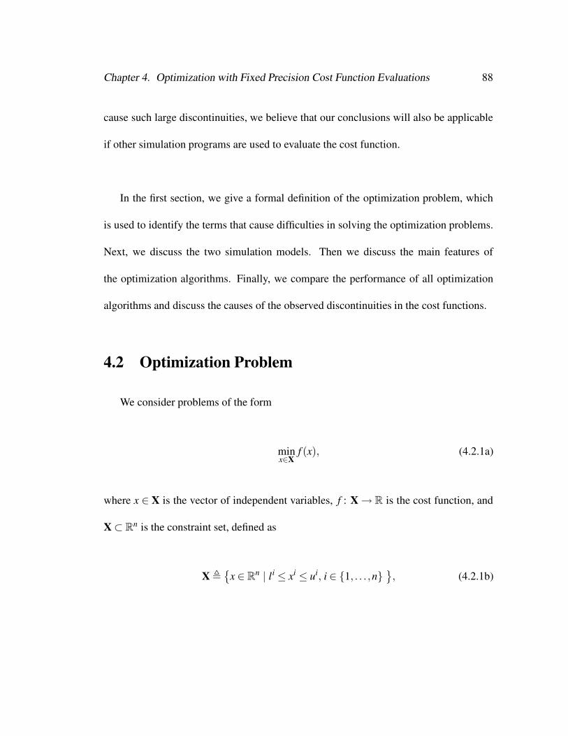
Chapter 4. Optimization with Fixed Precision Cost Function Evaluations 88
cause such large discontinuities, we believe that our conclusions will also be applicable
if other simulation programs are used to evaluate the cost function.
In the first section, we give a formal definition of the optimization problem, which
is used to identify the terms that cause difficulties in solving the optimization problems.
Next, we discuss the two simulation models. Then we discuss the main features of
the optimization algorithms. Finally, we compare the performance of all optimization
algorithms and discuss the causes of the observed discontinuities in the cost functions.
4.2 Optimization Problem
We consider problems of the form
minx∈X
f (x), (4.2.1a)
where x ∈ X is the vector of independent variables, f : X→ R is the cost function, and
X⊂ Rn is the constraint set, defined as
X ,
x ∈ Rn | li ≤ xi ≤ ui, i ∈ 1, . . . ,n, (4.2.1b)

Chapter 4. Optimization with Fixed Precision Cost Function Evaluations 89
with −∞≤ li < ui ≤ ∞, for all i ∈ 1, . . . ,n. The cost function f (·) is defined as
f (x) , F(z(x,1)
), (4.2.2)
where F : Rm→ R is once continuously differentiable but defined on the solution of a
coupled system of differential algebraic equations of the form
dz(x, t)dt
= h(x,µ, p(x)
), t ∈ [0, 1], (4.2.3a)
z(x,0) = z0(x), (4.2.3b)
γ(x,z(x, t),µ
)= 0, (4.2.3c)
where h : Rn×Rl×Rq→ Rm, z0 : Rn→ Rm and γ : Rn×Rm×Rl → Rl are once Lip-
schitz continuously differentiable in all arguments and the matrix with partial derivatives
γµ(·, ·, ·) is non-singular. The function h(·, ·, ·) describes the system dynamics, z(·, ·) is
the vector of state variables whose components are the room air and construction tem-
peratures (after the spatial discretization of the heat equation) and the heating, cooling
and lighting power. The algebraic variable µ is the solution of (4.2.3c) and its compo-
nents are state variables whose thermal capacities are assumed to be negligible, such
as the window glass temperatures. The elements of the vector p(·) ∈ Rq are the size
of the cooling coil, heating coil, and supply and return fan.1 Thus, the system (4.2.3)
1Clearly, the dependence of h(·, ·, ·) on p(·) can be eliminated by defining h(x,µ, p(x)) , h(x,µ), butwe find it convenient for our discussion to show explicitly the dependence on p(·).

Chapter 4. Optimization with Fixed Precision Cost Function Evaluations 90
is a mathematical model of a thermal building energy calculation. Under appropriate
assumptions, which are discussed in Chapter 2, one can show that (4.2.3) has a unique
once continuously differentiable solution. Several optimization algorithms that use ap-
proximate solutions of (4.2.3), and progressively decrease the approximation error as the
optimization approaches a solution, exist to solve (4.2.1), see Chapter 3.
However, in this Chapter, we are interested in the situation where EnergyPlus is
used to compute approximate numerical solutions of (4.2.3). EnergyPlus contains sev-
eral adaptive spatial and temporal grid generators, if-then-else logic and iterative
solvers that iterate until a convergence criterion is met. Due to these code features a
change in the independent variable x can cause a change in the sequence of code execu-
tions, which causes the approximate numerical solution of (4.2.3) to be discontinuous in
x.2 It is generally accepted in the simulation-based optimization community (Bertsekas,
1999; Gill et al., 1981; Polak, 1997) that in situations where (4.2.1) is solved using an
optimization algorithm that requires the cost function to be once continuously differen-
tiable, one needs to compute high-precision approximate solutions of (4.2.3). However,
in EnergyPlus the numerical solvers and grid generators are spread throughout the code
and most solver tolerance settings are fixed at compile time, in some cases at coarse pre-
cision. The implementation of the solvers is such that it does not seem possible to control
the numerical error. Thus, optimization algorithms that require smoothness may fail far
2Because z(·,1) and hence f (·) is discontinuous, f (·) may only have an infimum (i.e., a greatestlower bound) but no minimum even if X is compact. Thus, to be correct, (4.2.1a) should be replacedby infx∈X f (x). For simplicity, we will not make this distinction.

Chapter 4. Optimization with Fixed Precision Cost Function Evaluations 91
from a solution or may at best converge much slower. Consequently, we are interested in
how they perform compared to probabilistic population-based optimization algorithms
on rather smooth cost functions and on cost functions with large discontinuities.
4.3 Simulation Models
We will use two simulation models. The first is a simple simulation model that has 4
independent variables and no HVAC system simulation (the zone’s heating and cooling
loads are assumed to be met at each time step). The second is a detailed simulation model
that has 13 independent variables and a detailed HVAC system simulation. To determine
the size of the HVAC system of the detailed simulation model, EnergyPlus executes a
code that contains iterations. Thus, in the simple simulation model the component size
p(·) in (4.2.3a) is a constant, but in the detailed simulation model p(·) is a discontinuous
function of x.
In all optimization problems f (x) is the annual primary energy consumption for
lighting, fan, cooling and heating of a mid-story office floor. The exterior walls have
a U-value of 0.25W/(m2 K) and consist of (listed from outside to inside) 1cm wood
siding, 10cm insulation and 20cm concrete. The ceiling and floor consist of carpet, 5cm
concrete, insulation and 18cm concrete. Interior walls are 12cm brick. The windows are
low-emissivity double pane windows with Krypton gas fill and exterior shading device.
We use TMY2 weather data for Houston Intercontinental (TX), Chicago O’Hare (IL),

Chapter 4. Optimization with Fixed Precision Cost Function Evaluations 92
North
16 m6 m
2.7
m
3 m
2 m
1 m
(a) Simple office building.
(b) Detailed office building.
Figure 4.1: Buildings used in the numerical experiments.
and Seattle Tacoma (WA). Fig. 4.1 shows the office buildings.
4.3.1 Simple Simulation Model
The energy consumption of the gray shaded thermal zone in Fig. 4.1 is assumed to
be representative for the energy consumption of an elongated office building. Both win-
dows have an external shading device that is activated only during summer when the
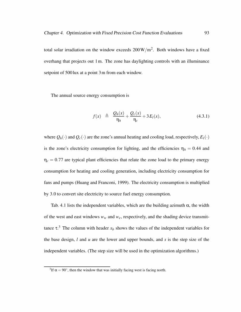
Chapter 4. Optimization with Fixed Precision Cost Function Evaluations 93
total solar irradiation on the window exceeds 200W/m2. Both windows have a fixed
overhang that projects out 1m. The zone has daylighting controls with an illuminance
setpoint of 500lux at a point 3m from each window.
The annual source energy consumption is
f (x) ,Qh(x)
ηh+
Qc(x)ηc
+3El(x), (4.3.1)
where Qh(·) and Qc(·) are the zone’s annual heating and cooling load, respectively, El(·)
is the zone’s electricity consumption for lighting, and the efficiencies ηh = 0.44 and
ηc = 0.77 are typical plant efficiencies that relate the zone load to the primary energy
consumption for heating and cooling generation, including electricity consumption for
fans and pumps (Huang and Franconi, 1999). The electricity consumption is multiplied
by 3.0 to convert site electricity to source fuel energy consumption.
Tab. 4.1 lists the independent variables, which are the building azimuth α, the width
of the west and east windows ww and we, respectively, and the shading device transmit-
tance τ.3 The column with header xb shows the values of the independent variables for
the base design, l and u are the lower and upper bounds, and s is the step size of the
independent variables. (The step size will be used in the optimization algorithms.)
3If α = 90, then the window that was initially facing west is facing north.

Chapter 4. Optimization with Fixed Precision Cost Function Evaluations 94
variable xb l u s Houston, TX Chicago, IL Seattle, WAsymbols best iterate x∗ best iterate x∗ best iterate x∗
(a) Optimization problems with simple simulation model and 4 independent variables.α 0 −180 180 10 92.81 86.25 87.50
wW 3 0.1 5.9 0.2 5.203 4.200 5.900wE 3 0.1 5.9 0.2 3.565 5.900 5.900τ 0.5 0.2 0.8 0.1 0.7964 0.5875 0.5375
Cost at base design, f (xb) in kWh/(m2 a) 208.2 185.1 164.9Cost at best iterate, f (x∗) in kWh/(m2 a) 190.3 155.8 138.0Maximum obtained reduction in % 8.58 15.82 16.32
(b) Optimization problems with detailed simulation model and 13 independent variables.wN 0.5 0 1 0.05 0.9969 1.000 1.000wW 0.5 0 1 0.05 0.1813 0.4000 0.5688oW 0.5 0 1 0.05 1.000 0.3500 0.6688wE 0.5 0 1 0.05 0.2125 0.3000 0.8813oE 0.5 0 1 0.05 1.000 0.4500 0.9656wS 0.5 0 1 0.05 0.6406 0.9500 1.000oS 0.5 0 1 0.05 1.000 0.1000 0.1438sW 200 100 600 25 398.4 400.0 312.5sE 200 100 600 25 406.3 450.0 200.0sS 200 100 600 25 375.0 575.0 600.0Tu 22 20 25 0.25 24.61 24.00 24.00Ti 22 20 25 0.25 22.98 24.75 24.95Td 15 12 18 0.25 12.00 12.00 12.00
Cost at base design, f (xb) in kWh/(m2 a) 165.4 130.1 114.6Cost at best iterate, f (x∗) in kWh/(m2 a) 141.5 115.7 95.82Maximum obtained reduction in % 14.45 11.02 16.41
Table 4.1: Variable symbols, initial value xb, lower bound l, upper bound u and stepsize s of the independent variable. The variable symbols are explained in the text. Thelast three columns show the best obtained iterates x∗. The bottom rows show the cor-responding cost function values and the obtained cost reductions for each optimizationproblem.
4.3.2 Detailed Simulation Model
We minimize the annual primary energy consumption for lighting, fan, cooling and
heating for the mid-story office floor shown in Fig. 4.1. Lighting and fan electricity are

Chapter 4. Optimization with Fixed Precision Cost Function Evaluations 95
multiplied by 3.0 and then added to the cooling and heating energy of the cooling and
heating coil. All exterior zones have daylighting control. The simulated HVAC system
is a VAV system with DX coil and outside-air economizer. The heating and cooling coil
capacities and the air flow rates are auto-sized by EnergyPlus. Tab. 4.1 lists the indepen-
dent variables. The variable wi, i ∈ N,W,E,S, linearly scales the window width and
height. The subscripts indicate north, west, east, and south, respectively. (The location
and shape of the windows are used in the daylighting calculations.) For the north and
south windows a value of 0 corresponds to a window that covers 13.6% of the facade
area and 1 corresponds to 64.8%. For the west and east windows a value of 0 corre-
sponds to a window that covers 20.4% of the facade area and 1 corresponds to 71.3%.
The variable oi, i ∈ W,E,S, scales the depth of the window overhangs. A value of
0 corresponds to a window overhang depth of 0.05 m (measured from the facade) and
1 corresponds to 1.05 m. The variable si, i ∈ W,E,S, is the setpoint for the shading
device in W/m2. If the total solar irradiation on the window exceeds si, then an external
shading device with a transmittance of 0.5 is activated. The variable Ti, i ∈ u, i, is
the setpoint for the zone air temperature for night cooling during summer and winter,
respectively, in C. The variable Td is the cooling design supply air temperature that is
used for the HVAC system sizing in C.

Chapter 4. Optimization with Fixed Precision Cost Function Evaluations 96
4.4 Optimization Algorithms
We compare the performance of nine optimization algorithms. In the following sec-
tion, we briefly describe the main features of all algorithms. For a more detailed descrip-
tion we refer the reader to Wetter and Wright (2003a) for the simple Genetic Algorithm
and to the GenOpt manual (Wetter, 2004) for all other algorithms, as well as to the ref-
erences cited therein. Since the performance of the optimization algorithms depends on
the algorithm parameters, we list all algorithm parameters, which may be used as initial
choices for similar problems. We did not tune the algorithm parameters but used values
which we believe will give good performance for the examined problems. A detailed ex-
planation of all parameters is beyond the scope of this Chapter, and we refer the reader
to Wetter and Wright (2003a) and to the GenOpt manual for details.
We will now describe the optimization algorithms used in the numerical experiments.
4.4.1 Coordinate Search Algorithm
The Coordinate Search algorithm searches along each coordinate direction for a de-
crease in f (·). Let k ∈ N be the iteration number, xk ∈ X be the current iterate, ∆k ∈Q+
be a scaling factor, called the mesh size factor, and s ∈ Rn be as in Tab. 4.1. Then, our
Coordinate Search algorithm tests if f (x′) < f (xk) for any x′ ∈ Lk, where
Lk ,
x ∈ X | x = xk±∆k si ei, i ∈ 1, . . . ,n. (4.4.1)

Chapter 4. Optimization with Fixed Precision Cost Function Evaluations 97
If there exists an x′ ∈ Lk that satisfies f (x′) < f (xk), then the algorithm sets xk+1 = x′,
∆k+1 = ∆k, and it replaces k by k + 1. Otherwise, it sets xk+1 = xk, decreases the mesh
size factor by setting ∆k+1 = ∆k/2, and it replaces k by k + 1. If ∆k is smaller than a
user-specified limit, the search stops.
The Coordinate Search algorithm is a member of the family of Generalized Pattern
Search (GPS) algorithms. For X = Rn, one can prove that any GPS method constructs a
sequence of iterates with stationary accumulation points if f (·) is continuously differen-
tiable and has bounded level sets (Audet and Dennis, 2003; Torczon, 1997). For a more
detailed description of GPS algorithms and an extension to constraint problems, see for
example Chapter 3, the paper by Audet and Dennis (2003) and the review by Kolda et al.
(2003).
For the numerical experiments, we used a mesh size divider of 2, an initial mesh size
exponent of 0, a mesh size exponent increment of 1 and 4 step reductions. Hence, ∆0 = 1
and, for the last iterations, ∆k = 1/16. Thus, the best iterate x∗ satisfies f (x∗) ≤ f (x′),
for all x′ ∈ x ∈ X | x = x∗±1/16 si ei, i ∈ 1, . . . ,n.
4.4.2 Hooke-Jeeves Algorithm
The Hooke-Jeeves algorithm is also a member of the family of GPS algorithms and
has therefore the same convergence properties on once continuously differentiable cost
functions as the Coordinate Search algorithm. It adjusts the mesh size factor ∆k using
the same algorithm as the Coordinate Search algorithm but, in addition to the search on

Chapter 4. Optimization with Fixed Precision Cost Function Evaluations 98
Lk, it also makes progressively bigger steps in the direction that has reduced the cost in
previous iterations. As in the Coordinate Search algorithm, the iterates of the Hooke-
Jeeves algorithm belong to a mesh of the form
M(x0, ∆k, s) ,
x0 +∆k
n
∑i=1
mi si ei | m ∈ Zn. (4.4.2)
The introduction of M(·, ·, ·) is convenient for the discussion of a modified Particle
Swarm Optimization algorithm and a hybrid algorithm below.
We used the same algorithm parameters for the Hooke-Jeeves algorithm as for the
Coordinate Search algorithm.
4.4.3 Particle Swarm Optimization Algorithms
Particle Swarm Optimization (PSO) algorithms are population-based probabilistic
optimization algorithms first proposed by Eberhart and Kennedy (Eberhart and Kennedy,
1995; Kennedy and Eberhart, 1995). At each iteration step, they compare the cost func-
tion value of a finite set of points, called particles. The change of each particle from
one iteration to the next is modeled based on the social behavior of flocks of birds or
schools of fish. Each particle attempts to change its location in X to a point where
it had a lower cost function value at previous iterations, which models cognitive be-
havior, and in a direction where other particles had a lower cost function value, which
models social behavior. Since our simulation model is computationally expensive, we
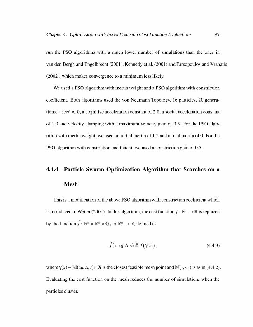
Chapter 4. Optimization with Fixed Precision Cost Function Evaluations 99
run the PSO algorithms with a much lower number of simulations than the ones in
van den Bergh and Engelbrecht (2001), Kennedy et al. (2001) and Parsopoulos and Vrahatis
(2002), which makes convergence to a minimum less likely.
We used a PSO algorithm with inertia weight and a PSO algorithm with constriction
coefficient. Both algorithms used the von Neumann Topology, 16 particles, 20 genera-
tions, a seed of 0, a cognitive acceleration constant of 2.8, a social acceleration constant
of 1.3 and velocity clamping with a maximum velocity gain of 0.5. For the PSO algo-
rithm with inertia weight, we used an initial inertia of 1.2 and a final inertia of 0. For the
PSO algorithm with constriction coefficient, we used a constriction gain of 0.5.
4.4.4 Particle Swarm Optimization Algorithm that Searches on a
Mesh
This is a modification of the above PSO algorithm with constriction coefficient which
is introduced in Wetter (2004). In this algorithm, the cost function f : Rn→R is replaced
by the function f : Rn×Rn×Q+×Rn→ R, defined as
f (x; x0,∆,s) , f(γ(x)
), (4.4.3)
where γ(x)∈M(x0,∆,s)∩X is the closest feasible mesh point and M(·, ·, ·) is as in (4.4.2).
Evaluating the cost function on the mesh reduces the number of simulations when the
particles cluster.

Chapter 4. Optimization with Fixed Precision Cost Function Evaluations 100
We run this algorithm with two different settings for the algorithm parameters. In the
first version, which we will call PSO on mesh (1), we used the same parameters as for
the PSO algorithm with constriction coefficient and, in addition, a mesh size divider of 2
and an initial mesh size exponent of 1. Thus, ∆ = 1/2 in (4.4.3). In the second version,
which we will call PSO on mesh (2), we increased the number of particles from 16 to
36 and increased the constriction gain from 0.5 to 1. This causes the particles to cluster
later in the search.
4.4.5 Hybrid Particle Swarm and Hooke-Jeeves Algorithm
This hybrid global optimization algorithm does a Particle Swarm Optimization on
a mesh for the first iterations, as described in the previous section. This is done for a
user-specified number of generations. Then, it starts the Hooke-Jeeves algorithm using
for the initial iterate the mesh point that attained the lowest cost function value. Since
the PSO algorithm evaluates f (·) only on a finite number of points in M(x0, ∆0, s)∩X,
the PSO search can be considered to be a global search of a GPS algorithm. Hence, this
hybrid algorithm is also a member of the family of GPS algorithms.
We run this algorithm with two different settings for the algorithm parameters. In the
first version, which we will call PSO and Hooke-Jeeves (1), we used the same settings
as for the algorithm PSO on mesh (1). In addition, we used, as for the Hooke-Jeeves
and the Coordinate Search algorithms, a mesh size exponent increment of 1. Because
∆0 = 1/2, we used 3 step reductions to obtain for the last iterations the same mesh size

Chapter 4. Optimization with Fixed Precision Cost Function Evaluations 101
factor as for the Hooke-Jeeves and the Coordinate Search algorithms, namely ∆k = 1/16.
In the second version, which we will call PSO and Hooke-Jeeves (2), we increased the
constriction gain from 0.5 to 1 to obtain a bigger spread in the particles for the late
generations, but we kept the number of particles at 16.
4.4.6 Simple Genetic Algorithm
Genetic Algorithms (GA) are algorithms that operate on a finite set of points, called
a population. The different populations are called generations. They are derived on the
principles of natural selection and incorporate operators for (1) fitness assignment, (2)
selection of points for recombination, (3) recombination of points, and (4) mutation of
a point. Our GA is an implementation of the simple GA described by Goldberg (1989),
but we use a Gray (Press et al., 1993) rather than a pure binary encoding to represent the
independent variables as a concatenated string of binary numbers.
The simple GA iterates either until a user-specified number of generations is ex-
ceeded, or until all iterates of the current generation have the same cost function value.
In the numerical experiments, we used a population size of 14, a maximum of 50
generations, 1 elite point and a probability for recombination and mutation of 1 and
0.02, respectively.
We selected a small population size because the number of independent variables is
small and because we expected the cost function to have no significant local minima. The
choice of a small population size was balanced by a high probability of recombination

Chapter 4. Optimization with Fixed Precision Cost Function Evaluations 102
and mutation. Small population sizes have also been used successfully in the solution of
other small scale building optimization problems, see Caldas and Norford (2002).
4.4.7 Simplex Algorithm of Nelder and Mead
The Simplex algorithm of Nelder and Mead is a derivative free optimization algo-
rithm. It constructs an n-dimensional simplex in the space of the independent variables.
The cost function is evaluated at each of the (n + 1) simplex vertices. In each iteration
step, the vertex with the highest cost function value is replaced by a new vertex. The
new vertex is obtained either by reflecting the vertex with the highest cost function value
at the centroid of the simplex, or by contracting and expanding the simplex. The Nelder
and Mead Simplex algorithm is an often used algorithm despite the well known fact that
it can fail to converge to a stationary point (see for example Kelley (1999b), Torczon
(1989), Kelley (1999a), Wright (1996), McKinnon (1998) and Lagarias et al. (1998)),
both in practice and theory, particularly if the dimension of independent variables is
large, say bigger than ten (Torczon, 1989). Several improvements to the Simplex algo-
rithm or algorithms that were motivated by the Simplex algorithm exist, see for example
Kelley (1999a,b), Torczon (1989) and Tseng (1999). However, here we used the original
Nelder-Mead algorithm, as described in Nelder and Mead (1965) with the extension of
O’Neill (1971) and, in some of the numerical experiments, a modification of the stopping
criteria, as described in the GenOpt manual.
For the numerical experiments, we used an accuracy of 0.01 and a step-size factor

Chapter 4. Optimization with Fixed Precision Cost Function Evaluations 103
of 0.1. In the experiments that are labeled Nelder-Mead (1), we modified the stopping
criterion as described in the GenOpt manual and prevented a new restart of the algorithm
during the ten iterations that followed a previous restart. In the experiments that are
labeled Nelder-Mead (2), we did not modify the stopping criterion and did not prevent a
restart of the algorithm. The second set of numerical experiments has been done because
the first set showed poor performance. However, the change in algorithm parameters did
not improve the performance.
4.4.8 Discrete Armijo Gradient Algorithm
We used the Discrete Armijo Gradient algorithm which is designed for the minimiza-
tion of once continuously differentiable functions. The algorithm is described in Polak
(1997) and in the GenOpt manual. It approximates gradients by finite differences, with
the difference increment reduced as the optimization progresses, and does line searches
using the Armijo step-size rule. If f (·) is once continuously differentiable and bounded
from below, then the Discrete Armijo Gradient algorithm constructs sequences with sta-
tionary accumulation points. However, the algorithm is sensitive to discontinuities in
f (·), and hence, we recommend to not use this algorithm if the simulation program con-
tains adaptive solvers with loose precision settings, such as EnergyPlus. However, since
the simple simulation model defines a cost function that has only small discontinuities,
we were interested in how this algorithm performs in solving the problems that use the
simple simulation model. As we will shortly see, it failed far from a solution.

Chapter 4. Optimization with Fixed Precision Cost Function Evaluations 104
We used the following algorithm parameters: α = 1/2, β = 0.8, γ = 0.1, k0 = 0,
k∗ =−10, lmax = 50, κ = 25, εm = 0.01 and εx = 0.05.
4.5 Numerical Experiments
The analysis presented here is in two parts. We will first compare the performance of
the different optimization algorithms and then examine the cause of the discontinuities
in the cost functions.
4.5.1 Comparison of the Optimization Results
For all optimizations, we used the optimization program GenOpt 2.0.0 (Wetter, 2001,
2004)4 and EnergyPlus 1.1.0. All computations were done on Linux computers using
the 2.4.20-8 kernel and AMD processors. On a 2.2 GHz processor, one simulation of
the simple model takes 14 seconds, and one simulation of the detailed model takes 2
minutes and 20 seconds. Thus, 300 simulations of the simple model (which is what
most optimization algorithms used in our experiments) takes 1 hour and 10 minutes, and
500 simulations of the detailed simulation model takes 19 hours and 30 minutes. The
overhead of the optimization algorithm and the file I/O is negligible.
We first need to define some measures that we will use to compare the optimization
results. Let xb ∈X be the value of the independent variables for the base design, as listed
4The Genetic Algorithm is currently only implemented in a development version.

Chapter 4. Optimization with Fixed Precision Cost Function Evaluations 105
in Tab. 4.1. For each optimization problem (i.e., for each simulation model with the
corresponding weather data), we denote, for each optimization algorithm, by x∗ ∈ X the
iterate with the lowest cost function value, and we denote for each optimization problem
by x ∈ X the iterate with the lowest cost function value obtained by any of the tested
optimization algorithms. Then, for each optimization problem, we define the normalized
cost reduction as
r(x∗) ,f (xb)− f (x∗)
f (xb), (4.5.1)
and we define the distance to the maximum obtained reduction as
d(r(x∗)
), r(x)− r(x∗) =
f (x∗)− f (x)f (xb)
. (4.5.2)
Thus, d(r(x∗)
)= 0 for the algorithm that achieves the biggest cost reduction.
Because of the discontinuities in the cost functions, we observed different behavior
of the optimization algorithms on the problems that used the simple simulation model
compared to the problems that used the detailed simulation model. The cost function,
if evaluated by the simple simulation model, is rather smooth, but, if evaluated by the
detailed simulation model, has discontinuities in the order of 2%, which makes opti-
mization with descent algorithms difficult.
Tab. 4.2 shows the normalized cost reduction, the distance to the maximum obtained
reduction and the number of simulations, and Fig. 4.2 shows a graphical representation

Chapter 4. Optimization with Fixed Precision Cost Function Evaluations 106
Houston, TX Chicago, IL Seattle, WAr(x∗) d
(r(x∗)
)m r(x∗) d
(r(x∗)
)m r(x∗) d
(r(x∗)
)m
Algorithm [%] [%] − [%] [%] − [%] [%] −
(a) Optimization problems with simple simulation model and 4 independent variables.PSOIW 8.44 0.14 316 15.42 0.41 316 16.11 0.21 314PSOCC 8.27 0.31 313 14.49 1.34 314 14.77 1.55 315PSOCC on a mesh (1) 8.27 0.31 169 14.57 1.25 160 14.89 1.43 146PSOCC on a mesh (2) 8.47 0.12 672 15.75 0.07 673 16.23 0.09 652Nelder-Mead (1) 8.58 0 259 15.71 0.11 672 16.18 0.14 1232Nelder-Mead (2) 8.58 0 226 15.71 0.11 902 16.25 0.07 1451PSO and Hooke-Jeeves (1) 8.58 0.01 242 15.82 0 237 16.30 0.02 215PSO and Hooke-Jeeves (2) 8.56 0.02 326 15.74 0.08 371 16.32 0 358Hooke-Jeeves 8.58 0.01 103 15.82 0 113 16.30 0.02 97Coordinate Search 8.58 0.01 105 15.82 0 119 16.30 0.02 116Simple GA 8.53 0.05 194 15.52 0.31 185 16.23 0.09 176Discrete Armijo Gradient 7.93 0.66 315 13.08 2.75 364 14.95 1.37 216
(b) Optimization problems with detailed simulation model and 13 independent variables.PSOIW 13.91 0.54 317 10.63 0.39 317 15.39 1.03 318PSOCC 11.97 2.49 313 9.66 1.37 314 14.18 2.23 317PSOCC on a mesh (1) 12.17 2.28 195 9.68 1.34 209 14.20 2.22 242PSOCC on a mesh (2) 13.49 0.96 710 10.39 0.63 712 15.84 0.57 707Nelder-Mead (1) 14.09 0.36 2330 4.27 6.76 1228 15.59 0.82 5846Nelder-Mead (2) 13.98 0.48 1578 – – – – – –PSO and Hooke-Jeeves (1) 14.16 0.29 653 10.94 0.09 755 16.18 0.23 843PSO and Hooke-Jeeves (2) 14.45 0 740 10.96 0.06 669 16.41 0 889Hooke-Jeeves 14.27 0.18 555 5.93 5.10 600 16.32 0.09 574Coordinate Search 9.60 4.86 430 4.74 6.29 552 13.04 3.37 501Simple GA 14.06 0.40 586 11.02 0 592 16.35 0.07 583
Table 4.2: Normalized cost reduction r(x∗), distance to the maximum obtained costreduction d
(r(x∗)
)and number of simulations m for all optimization problems.
of the distance to the maximum obtained cost reduction and the required number of
simulations for each optimization problem.
We see that if the detailed simulation model is used, then the Coordinate Search
algorithm tends to fail far from the minimum. On the same problems, the Hooke-Jeeves
algorithm jammed less often compared to the Coordinate Search algorithm, which may
be due to the larger steps that are taken in the global exploration.
All non-hybrid PSO algorithms come close to the minimum with a low number of

Chapter 4. Optimization with Fixed Precision Cost Function Evaluations 107
simulations. By restricting the iterates of the PSO algorithm with constriction coefficient
to the mesh M(x0,∆,s), the number of simulations could be reduced by 50% for the
problem with 4 independent variables and by 30% for the problem with 13 independent
variables. Restricting the iterates to the mesh does not significantly affect the accuracy as
we can see by comparing the results of the PSOCC and the PSO on mesh (1) algorithm,
which both use the same algorithm parameters. However, in the PSO algorithm that
searches on a mesh, increasing the number of particles from 16 to 36 and increasing the
constriction gain from 0.5 to 1 prevented the particles to cluster early in the search and
yielded larger cost reductions at the expense of three to four times more simulations.
The simple GA, however, got consistently closer to the minimum than the PSO al-
gorithms with a comparable number of simulations, except for one problem that used
the simple simulation model. In this case, however, the difference in cost reduction is
insignificant.
The overall best cost reductions has been achieved by the hybrid Particle Swarm and
Hooke-Jeeves algorithm although with a higher number of simulations than the simple
GA. For the hybrid algorithm, increasing the constriction gain from 0.5 to 1.0 did, in
our experiments, only slightly change the results. We observed, however, that with a
higher constriction gain the particles are more spread out in the early generations, which
increases the chance to find a global minimum if the cost function has several minima.
The Nelder-Mead algorithm did not perform well on our test problems. It required
a high number of simulations, and in one test case it failed far from the minimum. We

Chapter 4. Optimization with Fixed Precision Cost Function Evaluations 108
believe that, in addition to the problems discussed in the literature (Kelley, 1999a,b;
Lagarias et al., 1998; McKinnon, 1998; Torczon, 1989; Wright, 1996), some of the prob-
lems we observed when solving the optimization problems that used the detailed sim-
ulation model may have been caused by the stopping criterion. The stopping criterion
described by Nelder and Mead (1965), which is the one implemented in GenOpt, re-
quires the variance of the function values at the simplex vertices to be smaller than a
prescribed limit. However, if f (·) has large discontinuities, then this stopping criterion
may never be satisfied.
The Discrete Armijo Gradient algorithm failed on the simple problem far from the
minimum. This is not surprising because the algorithm is sensitive to discontinuities
in the cost function. We recommend to not use this algorithm if EnergyPlus is used to
evaluate the cost function.
In summary, the simple GA got close to a solution with a low number of simulations.
The hybrid Particle Swarm and Hooke-Jeeves algorithm achieved the biggest cost re-
duction but required more simulations. Whether the increased number of simulations is
justified depends on the savings due to a better solution and the expenses of a higher com-
putation time. However, one advantage of the hybrid algorithm is that the global search
of the PSO algorithm increases the chance to get close to the global minimum rather than
only a local minimum, and the Hooke-Jeeves algorithm then refines the search locally.
If the discontinuities in the cost function are small, then the Hooke-Jeeves algorithm
achieved a good reduction in cost and required only few iterations.

Chapter 4. Optimization with Fixed Precision Cost Function Evaluations 109
+ + ! "
#
+$%& ' ( )*+,+
-./0
12
+345 6 7 89:;<=>? +
@ A+BCD E FGH IJ + KLMN O
P
+QRS T U VWXY+
Z[\]
^_
+`ab c d efghijkl +
mnumber of simulations, m
0 200 400 600 800 1000 1200 1400 1600
d(r(x∗)
)
0.0
0.01
0.02
0.03
LegendnDiscrete Armijo Gradient
+ simple GAo Coordinate Searchpq Hooke-JeevesrPSO and Hooke-JeevesstNelder-Mead
+ PSOCCuv PSOCC on a meshw PSOIW
(a) Optimization problems with simple simulation model and 4 independent variables.
+
x
yz| ~ +
+
+ +
+¡
number of simulations, m
0 1000 2000 3000 4000 5000 6000
d(r(x∗)
)
0.0
0.01
0.02
0.03
0.04
0.05
0.06
0.07 Legend+ simple GA¢ Coordinate Search£¤ Hooke-Jeeves¥ PSO and Hooke-Jeeves¦§ Nelder-Mead
+ PSOCC¨© PSOCC on a meshª PSOIW
(b) Optimization problems with detailed simulation model and 13 independent variables.
Figure 4.2: Number of simulations vs. distance to the maximum obtained costreduction.

Chapter 4. Optimization with Fixed Precision Cost Function Evaluations 110
4.5.2 Discontinuities in the Cost Function
We observed that EnergyPlus computes for the detailed simulation model an energy
consumption that has large discontinuities. Some of the discontinuities are caused by
the adaptive grid generators – such as the ones used in computing the daylighting illu-
minance or in doing the variable time-step integration – some are caused by iterative
solvers which fail to compute an accurate approximate solution and some are caused by
programming errors.
Due to these discontinuities, for the optimization problem with the detailed simula-
tion model and Chicago’s weather data, the Hooke-Jeeves algorithm achieved only half
of the cost reduction that was obtained by other algorithms. For this numerical experi-
ment, we will now show the change in cost in a one-dimensional subspace of X⊂ R13.
In particular, we will perturb one component of the independent variable and plot the
change in cost function value. We will first introduce some notation. Let x∗HJ ∈ X⊂R13
denote the iterate with the lowest cost function value of the Hooke-Jeeves algorithm, let
Tu ∈ R denote the room setpoint temperature for night cooling during summer, and let
eTu ∈ R13 denote the coordinate vector along Tu. We define T ∗u,HJ , 〈x∗HJ,eTu〉 and we
define the normalized change in cost with respect to Tu as
δ(Tu) ,f(x∗HJ +(Tu−T ∗u,HJ)eTu
)
f (x∗HJ). (4.5.3)
In Fig. 4.3 we show δ(Tu) for Tu ∈ [21.9, 22.1] using 1201 equidistant support points.
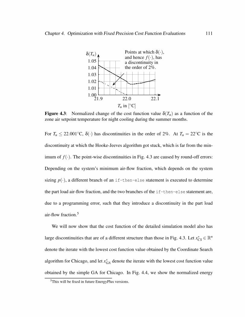
Chapter 4. Optimization with Fixed Precision Cost Function Evaluations 111
««« « « « « « « « « « « « « « « « « « « « ««« « « « « « « « « « « « « « « « « « « « « « « « « « «« «« « « « « ««« « « « « « « « « « « « « « « « « « ««« ««« « « « « « « « « « « « ««« « « « « « « « « « « « « « ««« ««« « « « « « « « « « « « « « « « « « « « « « « « « « « « « ««« « « « « « « « « « « « « « « « « « « « « « « « « « « « « « « « « « « « « « « « « « « « « « ««« « « « « « « « ««« « « « « « « « « « « ««« « « « « « « « « « « « « « « « « « « « « « « « « « « « « « « « « « « « « « « « « « « « « « « « « « ««« « « « « « « « « ««« « ««« « « « « « « « « « « « « « « « « « « « « « « « « « « « « « « « « « « « « ««« « ««« « « « « ««« « « « « « « « « « « « « « « « « « « « « « « « « « « « « « « « « « « « « « « « « ««« « ««««« « « « « ««« « « « ««« ««« « « « « « « « ««« « « « « « « « ««« « « « « « « « « « « « « « « « « « « « ««« « « « « « « « «« «« « « « « « « « « « « « « « « « « « « « ««« « « « « « « « « « « « « « « « « « « «« «« « « « « « « « « « « « « « « « « « « « « « « ««««« « « « « « ««« « « « « « « « « « ««« « « « « « « « « « « « « ««« « « « « « « « « « « « « « « « « « « « « « « « « « ««« « « « « « « « « « « « ««« « « « ««« « « « « « « « « « « « « « « « « « « « « « « « « « « « « « « « « « « « « « « « « « « « « « « « « « « « « « « « « « « « « « « « « « « « « « « « « « « « « « « « « « « « « « « « « « « « « « « « « « « « « « « « « « « « « « « « « « « « « « « « « « « « « « « « « « « « « « « « « « « « « « « « « « « « « « « « « « « « « « « « « « « « « « « « « « « « « « « « « « « « « « « « « « « « « « « « « « « « « « « « « « « « « « « « « « « « « « « « « « « « « « « « « « « « « « « « « « « « « « « « « « « « « « « « « « « « « « « « « « « « « « « « « « « « « « « « « « « « « « « « « « « « « « « « « « « « « « « « « « « « « « « « « « « « « « « « « « « « « « « « « « « « « « « « « « « « « « « « « « « « « « « « « « « « « « « « « « « « « « « « « « « « « « « « « « « « « « « « « « « « « « « « « « « « « « « « « « « « « « « « « « « « « « « « « « « « « « « « « « « « « « « « « « « « « « « « « « « « « « « « « « « « « « « « « « « « « « « « « « « « « « « « « « « « « « « « « « « « « « « « « « « « « « « « « « « « « « « « « « « « « « « « « « « « « « « « « « « « « « « « « « « « « « « « « « « « « « « « « « « « « « « « « « « « « « « « « « « « « « « « « « « « « « « « « « « « « « « « « « « « « « « « « « « « « « « « « «
Tu in [C]
δ(Tu)
21.9 22.0 22.11.001.011.021.031.041.05
Points at which δ(·),and hence f (·), hasa discontinuity inthe order of 2%.
Figure 4.3: Normalized change of the cost function value δ(Tu) as a function of thezone air setpoint temperature for night cooling during the summer months.
For Tu ≤ 22.001C, δ(·) has discontinuities in the order of 2%. At Tu = 22C is the
discontinuity at which the Hooke-Jeeves algorithm got stuck, which is far from the min-
imum of f (·). The point-wise discontinuities in Fig. 4.3 are caused by round-off errors:
Depending on the system’s minimum air-flow fraction, which depends on the system
sizing p(·), a different branch of an if-then-else statement is executed to determine
the part load air-flow fraction, and the two branches of the if-then-else statement are,
due to a programming error, such that they introduce a discontinuity in the part load
air-flow fraction.5
We will now show that the cost function of the detailed simulation model also has
large discontinuities that are of a different structure than those in Fig. 4.3. Let x∗CS ∈ Rn
denote the iterate with the lowest cost function value obtained by the Coordinate Search
algorithm for Chicago, and let x∗GA denote the iterate with the lowest cost function value
obtained by the simple GA for Chicago. In Fig. 4.4, we show the normalized energy
5This will be fixed in future EnergyPlus versions.

Chapter 4. Optimization with Fixed Precision Cost Function Evaluations 112
¬ ¬ ¬ ¬ ¬ ¬ ¬ ¬ ¬ ¬ ¬ ¬ ¬ ¬ ¬ ¬ ¬ ¬ ¬ ¬ ¬ ¬ ¬ ¬ ¬ ¬ ¬ ¬ ¬ ¬ ¬ ¬ ¬ ¬ ¬ ¬ ¬ ¬ ¬ ¬ ¬ ¬ ¬ ¬ ¬ ¬ ¬ ¬ ¬ ¬ ¬ ¬ ¬ ¬ ¬ ¬ ¬ ¬ ¬ ¬ ¬ ¬ ¬ ¬ ¬ ¬ ¬ ¬ ¬ ¬ ¬ ¬ ¬ ¬ ¬ ¬ ¬ ¬ ¬ ¬ ¬ ¬ ¬ ¬ ¬ ¬ ¬ ¬ ¬ ¬ ¬ ¬ ¬ ¬ ¬ ¬ ¬ ¬ ¬ ¬ ¬ ¬ ¬ ¬ ¬ ¬ ¬ ¬ ¬ ¬ ¬ ¬ ¬ ¬ ¬ ¬ ¬ ¬ ¬ ¬ ¬ ¬ ¬ ¬ ¬ ¬ ¬ ¬ ¬ ¬ ¬ ¬ ¬ ¬ ¬ ¬ ¬ ¬ ¬ ¬ ¬ ¬ ¬ ¬ ¬ ¬ ¬ ¬ ¬ ¬ ¬ ¬ ¬ ¬ ¬ ¬ ¬ ¬ ¬ ¬ ¬ ¬ ¬ ¬ ¬ ¬ ¬ ¬ ¬ ¬ ¬ ¬ ¬ ¬ ¬ ¬ ¬ ¬ ¬ ¬ ¬ ¬ ¬ ¬ ¬ ¬ ¬ ¬ ¬ ¬ ¬ ¬ ¬ ¬ ¬ ¬ ¬ ¬ ¬ ¬ ¬scalar λ
Total primary energy
0.6 0.7 0.8 0.9 1.01.001.011.021.031.041.051.06
scalar λ
Fan energy
0.6 0.7 0.8 0.9 1.01.0
1.1
1.2
1.3
1.4
® ® ® ® ® ® ® ® ® ® ® ® ® ® ® ® ® ® ® ® ® ® ® ® ® ® ® ® ® ® ® ® ® ® ® ® ® ® ® ® ® ® ® ® ® ® ® ® ® ® ® ® ® ® ® ® ® ® ® ® ® ® ® ® ® ® ® ® ® ® ® ® ® ® ® ® ® ® ® ® ® ® ® ® ® ® ® ® ® ® ® ® ® ® ® ® ® ® ® ® ® ® ® ® ® ® ® ® ® ® ® ® ® ® ® ® ® ® ® ® ® ® ® ® ® ® ® ® ® ® ® ® ® ® ® ® ® ® ® ® ® ® ® ® ® ® ® ® ® ® ® ® ® ® ® ® ® ® ® ® ® ® ® ® ® ® ® ® ® ® ® ® ® ® ® ® ® ® ® ® ® ® ® ® ® ® ® ® ® ® ® ® ® ® ® ® ® ® ® ® ®¯ ¯ ¯ ¯ ¯ ¯ ¯ ¯ ¯ ¯ ¯ ¯ ¯ ¯ ¯ ¯ ¯ ¯ ¯ ¯ ¯ ¯ ¯ ¯ ¯ ¯ ¯ ¯ ¯ ¯ ¯ ¯ ¯ ¯ ¯ ¯ ¯ ¯ ¯ ¯ ¯ ¯ ¯ ¯ ¯ ¯ ¯ ¯ ¯ ¯ ¯ ¯ ¯ ¯ ¯ ¯ ¯ ¯ ¯ ¯ ¯ ¯ ¯ ¯ ¯ ¯ ¯ ¯ ¯ ¯ ¯ ¯ ¯ ¯ ¯ ¯ ¯ ¯ ¯ ¯ ¯ ¯ ¯ ¯ ¯ ¯ ¯ ¯ ¯ ¯ ¯ ¯ ¯ ¯ ¯ ¯ ¯ ¯ ¯ ¯ ¯ ¯ ¯ ¯ ¯ ¯ ¯ ¯ ¯ ¯ ¯ ¯ ¯ ¯
¯ ¯ ¯ ¯ ¯ ¯ ¯ ¯ ¯ ¯ ¯ ¯ ¯ ¯ ¯ ¯ ¯ ¯ ¯ ¯ ¯ ¯ ¯ ¯ ¯ ¯ ¯ ¯ ¯ ¯ ¯ ¯ ¯ ¯ ¯ ¯ ¯ ¯ ¯ ¯ ¯ ¯ ¯ ¯ ¯ ¯ ¯ ¯ ¯ ¯ ¯ ¯ ¯ ¯ ¯ ¯ ¯ ¯ ¯ ¯ ¯ ¯ ¯ ¯ ¯ ¯ ¯ ¯ ¯ ¯ ¯ ¯ ¯ ¯ ¯ ¯ ¯ ¯ ¯ ¯ ¯ ¯ ¯ ¯ ¯ ¯ ¯
scalar λ
Cooling and heating energy
0.6 0.7 0.8 0.9 1.00.85
0.90
0.95
1.00
1.05 cooling
heating
° ° ° ° ° ° ° ° ° ° ° ° ° ° ° ° ° ° ° ° ° ° ° ° ° ° ° ° ° ° ° ° ° ° ° ° ° ° ° ° ° ° ° ° ° ° ° ° ° ° ° ° ° ° ° ° ° ° ° ° ° ° ° ° ° ° ° ° ° ° ° ° ° ° ° ° ° ° ° ° ° ° ° ° ° ° ° ° ° ° ° ° ° ° ° ° ° ° ° ° ° ° ° ° ° ° ° ° ° ° ° ° ° ° ° ° ° ° ° ° ° ° ° ° ° ° ° ° ° ° ° ° ° ° ° ° ° ° ° ° ° ° ° ° ° ° ° ° ° ° ° ° ° ° ° ° ° ° ° ° ° ° ° ° ° ° ° ° ° ° ° ° ° ° ° ° ° ° ° ° ° ° ° ° ° ° ° ° ° ° ° ° ° ° ° ° ° ° ° ° ° ° ° ° ° ° ° ° ° ° ° ° ° ° ° ° ° ° ° ° ° ° ° ° ° ° ° ° ° ° ° ° ° ° ° ° ° ° ° ° ° ° ° ° ° ° ° ° ° ° ° ° ° ° ° ° ° ° ° ° ° ° ° ° ° ° ° ° ° ° ° ° ° ° ° ° ° ° ° ° ° ° ° ° ° ° ° ° ° ° ° ° ° ° ° ° ° ° ° ° ° ° ° ° ° ° ° ° ° ° ° ° ° ° ° ° ° ° ° ° ° ° ° ° ° ° ° ° ° ° ° ° ° ° ° ° ° ° ° ° ° ° ° ° ° ° ° ° ° ° ° ° ° ° ° ° ° ° ° ° ° ° ° ° ° ° ° ° ° ° ° ° ° ° ° ° ° ° ° ° ° ° ° ° ° ° ° ° ° ° ° ° ° ° ° ° ° ° ° ° ° ° ° ° ° ° ° ° ° ° ° ° ° ° ° ° ° ° ° ° ° ° ° ° ° ° ° ° ° ° ° ° ° ° ° ° ° ° ° ° ° ° ° ° ° ° ° ° ° ° ° ° ° ° ° ° ° ° ° ° ° ° ° ° ° ° ° ° ° ° ° ° ° ° ° ° ° ° ° ° ° ° ° ° ° ° ° ° ° ° ° ° ° ° ° ° ° ° ° ° °scalar λ
Lighting energy
0 0.2 0.4 0.6 0.8 1.01.00001.00251.00501.00751.01001.0125
Figure 4.4: Normalized cost function value f (x(λ))/ f (x(1)) and primary energy con-sumption for fan, cooling, heating and lighting, normalized by dividing it by the valueat the minimum point of the simple GA. The functions are evaluated on the line be-tween the minimum point obtained by the Coordinate Search algorithm (at λ = 0) andthe minimum point obtained by the simple GA (at λ = 1) for Chicago, IL.
consumption for total primary energy, fan, cooling, heating and lighting energy. The nor-
malized energy consumption is shown along part of the line x(λ) , x∗CS +λ(x∗GA− x∗CS
).
That is, x(0) = x∗CS and x(1) = x∗GA. The graph shows discontinuities of the total primary
energy consumption in the order of 1%. Clearly, such large discontinuities can cause
optimization algorithms that require smoothness of the cost function to fail far from a
minimum.
The biggest discontinuities seem to be caused by the fan sizing. At λ = 0.827, the

Chapter 4. Optimization with Fixed Precision Cost Function Evaluations 113
fan energy changes by 4% and consequently the cooling and heating energy is also dis-
continuous at this point. However, at λ = 0.931, the cooling energy changes by 1.2%
while the fan energy is smooth around this point. While such a discontinuity is small if
one is only interested in the cooling sizing in a simulation study, it can cause problems in
optimization and sensitivity studies, particularly if the cooling energy contributes much
to the cost function. The discontinuities in lighting energy are small (the lighting energy
does not depend on the fan, cooling or heating energy). We believe that the disconti-
nuities in the lighting energy are caused by a change in the spatial discretization that is
used in computing the daylight illuminance. We further believe that the large discontinu-
ities in the fan, heating and cooling energy are caused by the system auto-sizing, which
we expect to compute a low-precision approximate solution to p(x), which will then be
used in (4.2.3) for the whole interval of time integration. In fact, the system sizing is
done by first repetitively simulating a so-called warm-up day until some state variables
do not change more than a tolerance which is fixed at compile time, and then one day is
simulated to determine p(·). This is done for a winter and a summer day. Thus, a change
in x can cause a discrete change in the number of warm-up days, and hence in the initial
state z0(x) and consequently in the system size p(x).

Chapter 4. Optimization with Fixed Precision Cost Function Evaluations 114
4.6 Conclusion
We observed that in the optimization problems that used the detailed simulation
model with auto-sizing of the HVAC components, the cost function has discontinuities in
the order of 2%. On such problems optimization algorithms that require smoothness of
the cost function are likely to fail far from a solution, which is what we indeed observed
in our numerical experiments. Such discontinuities make optimization difficult and can
lead to limited economic gains. This can be prevented if the solvers are implemented
in such a way that the approximation error can be controlled, and if the simulation pro-
gram is written in such a way that the approximate solutions of the differential algebraic
equations converge to a smooth function as the precision of the numerical solvers is in-
creased. We developed a building energy simulation program that allows such an error
control. It is presented in Chapter 2.
The biggest cost reduction has been obtained with the hybrid Particle Swarm and
Hooke-Jeeves algorithm. If a user is willing to accept a slight decrease in accuracy at
the benefit of fewer simulations, then the simple GA is a good choice. However, due to
the stochastic operators, the PSO and the simple GA can occasionally fail to get close
to a solution, particularly if the number of simulations is small. In such situations, the
second search in a hybrid algorithm can further decrease the cost. However, with our
limited number of numerical experiments, we could not determine how big the risk of
failing is.

Chapter 4. Optimization with Fixed Precision Cost Function Evaluations 115
For neither of the problems that we examined do we recommend using either the
Nelder-Mead or the Discrete Armijo Gradient algorithm.

116
Bibliography
Abramson, M. A. (2002). Pattern Search Algorithms for Mixed Variable General Con-
strained Optimization Problems. PhD thesis, Rice University, Houston, TX.
Al-Homoud, M. S. (1997). Optimum thermal design of office buildings. International
Journal of Energy Research, 21:941–957.
Arasteh, D. K., Finlayson, E. U., and Huizenga, C. (1994). WINDOW 4.1: Program
description. Technical Report LBL-35298, Lawrence Berkeley National Laboratory,
Berkeley, CA, USA.
Arasteh, D. K., Reilly, M. S., and Rubin, M. D. (1989). A versatile procedure for calcu-
lating heat transfer through windows. In ASHRAE Transactions, volume 95.2, pages
755–765.
ASHRAE (1989). Fundamentals. American Society of Heating, Refrigeration and Air-
Conditioning Engineers.

Bibliography 117
ASHRAE (2001). ANSI/ASHRAE Standard 140-2001, Standard method of test for the
evaluation of building energy analysis computer programs.
Audet, C. and Dennis, Jr., J. E. (2000a). Pattern search algorithms for mixed variable
programming. SIAM Journal on Optimization, 11(3):573–594.
Audet, C. and Dennis, Jr., J. E. (2000b). A pattern search filter method for nonlinear pro-
gramming without derivatives. Technical Report TR 00-09, Rice University, Houston,
Department of Computational and Applied Mathematics.
Audet, C. and Dennis, Jr., J. E. (2003). Analysis of generalized pattern searches. SIAM
Journal on Optimization, 13(3):889–903.
Baum, D. R., Rushmeier, H. E., and Winget, J. M. (1989). Improving radiosity solu-
tions through the use of analytically determined form-factors. Computer Graphics,
23(3):325–334.
Berdahl, P. and Fromberg, R. (1982). The thermal radiance of clear skies. Solar Energy,
29:299–314.
Berdahl, P. and Martin, M. (1984). Emissivity of clear skies. Solar Energy, 32:663–664.
Bertsekas, D. P. (1999). Nonlinear Programming. Athena Scientific, Belmont, MA,
USA, 2nd edition.
Bjorsell, N., Bring, A., Eriksson, L., Grozman, P., Lindgren, M., Sahlin, P., Shapovalov,
A., and Vuolle, M. (1999). IDA indoor climate and energy. In Nakahara, N., Yoshida,

Bibliography 118
H., Udagawa, M., and Hensen, J., editors, Proc. of the 6-th IBPSA Conference, pages
1035–1042, Kyoto, Japan.
BLAST (1999). BLAST 3.0 Users Manual. University of Illinois, Urbana-Champaign,
IL, Department of Mechanical and Industrial Engineering, Building Systems Labora-
tory.
Booker, A., Dennis, Jr., J. E., Frank, P., Serafini, D., and Torczon, V. (1998). Opti-
mization using surrogate objectives on a helicopter test example. In Borggaard, J. T.,
Burns, J., Cliff, E., and Schreck, S., editors, Computational Methods in Optimal De-
sign and Control, volume 24 of Progress in Systems and Control Theory, pages 49–58.
Birkhauser, Boston.
Booker, A. J., Dennis, Jr., J. E., Frank, P. D., Serafini, D. B., Torczon, V., and Trosset,
M. W. (1999). A rigorous framework for optimization of expensive functions by
surrogates. Structural Optimization, 17(1):1–13.
Brenan, K. E., Campbell, S. L., and Petzold, L. R. (1989). Numerical Solution of Initial-
Value Problems in Differential-Algebraic Equations. North-Holland.
Brown, P. N., Hindmarsh, A. C., and Petzold, L. R. (1994). Using Krylov methods in
the solution of large-scale differential-algebraic systems. SIAM Journal on Scientific
Computing, 15:1467–1488.
Brown, P. N., Hindmarsh, A. C., and Petzold, L. R. (1998). Consistent initial condition

Bibliography 119
calculation for differential-algebraic systems. SIAM Journal on Scientific Computing,
19(5):1495–1512.
Bryan, H. J. and Clear, R. D. (1981). Calculating interior daylight illumination with
a programmable hand calculator. Journal of the Illuminating Engineering Society,
10(4):219–227.
Caldas, L. G. and Norford, L. K. (2002). A design optimization tool based on a genetic
algorithm. Automation in Construction, 11(2):173–184.
Carroll, W. L. (2003). Personal communication.
Choi, T. D. and Kelley, C. T. (2000). Superlinear convergence and implicit filtering.
SIAM Journal on Optimization, 10(4):1149–1162.
Choudhary, R. (2004). A Hierarchical Optimization Framework for Simulation-Based
Architectural Design. PhD thesis, University of Michigan.
Choudhary, R., Malkawi, A., and Papalambros, P. Y. (2003). A hierarchical design
optimization framework for building performance analysis. In Augenbroe, G. and
Hensen, J., editors, Proc. of the 8-th IBPSA Conference, Eindhoven, NL.
Clarke, F. H. (1990). Optimization and nonsmooth analysis. Society for Industrial and
Applied Mathematics (SIAM), Philadelphia, PA.
Clarke, J. A. (2001). Energy Simulation in Building Design. Butterworth-Heinemann,
Oxford, UK, 2nd edition.

Bibliography 120
Coddington, E. A. and Levinson, N. (1955). Theory of ordinary differential equations.
McGraw-Hill Book Company, Inc., New York-Toronto-London.
Crawley, D. B., Lawrie, L. K., Winkelmann, F. C., Buhl, W. F., Huang, Y. J., Pedersen,
C. O., Strand, R. K., Liesen, R. J., Fisher, D. E., Witte, M. J., and Glazer, J. (2001).
EnergyPlus: creating a new-generation building energy simulation program. Energy
and Buildings, 33(4):443–457.
Cuzzillo, B. R. and Pagni, P. J. (1998). Thermal breakage of double-pane glazing by fire.
J. of Fire Prot. Engr., 9(1):1–11.
Dennis, Jr., J. E. and Torczon, V. (1991). Direct search methods on parallel machines.
SIAM Journal on Optimization, 1(4):448–474.
Dennis, Jr., J. E. and Torczon, V. (1997). Managing approximation models in optimiza-
tion. In Alexandrov, N. M. and Hussaini, M. Y., editors, Multidisciplinary Design
Optimization: State of the Art, ICASE/NASA Langley Workshop on Multidisciplinary
Optimization, pages 330–347. SIAM.
Durand, F., Drettakis, G., and Puech, C. (1999). Fast and accurate hierarchical radiosity
using global visibility. ACM Transactions on Graphics (TOG), 18(2):128–170.
Eberhart, R. C. and Kennedy, J. (1995). A new optimizer using particle swarm theory. In
Sixth International Symposium on Micro Machine and Human Science, pages 39–43,
Nagoya, Japan. IEEE.

Bibliography 121
Evans, L. C. (1998). Partial differential equations. American Mathematical Society.
Finkel, D. E. (2003). DIRECT Optimization Algorithm User Guide. North Carolina
State University, Center for Research in Scientific Computation, Raleigh, NC.
Finlayson, E. U., Arasteh, D. K., Huizenga, C., Rubin, M. D., and Reilly, M. S. (1993).
WINDOW 4.0: Documentation of calculation procedures. Technical Report LBL-
33943, Lawrence Berkeley National Laboratory, Berkeley, CA, USA.
Fontoynont, M., Laforgue, P., Mitanchey, R., Aizlewood, M., Butt, J., Carroll, W., Hitch-
cock, R., Erhorn, H., Boer, J. D., Dirksmoller, M., Michel, L., Paule, B., Scartezzini,
J. L., Bodart, M., and Roy, G. (1999). IEA SHC Task 21/ECBCS Annex 29, Daylight
in buildings, Subtask C1: Validation of daylighting simulation programmes. Technical
Report T21/C1-/FRA/99-11, International Energy Agency.
Gablonsky, J. M. and Kelley, C. T. (2001). A locally-biased form of the DIRECT algo-
rithm. Journal of Global Optimization, 21(1):27–37.
Gill, P. E., Murray, W., and Wright, M. H. (1981). Practical optimization. Academic
Press Inc. [Harcourt Brace Jovanovich Publishers], London.
Goldberg, D. (1989). Genetic Algorithm in Search, Optimization, and Machine Learn-
ing. Adisson-Wesley.
Greenhalgh, D. and Marshall, S. (2000). Convergence criteria for genetic algorithms.
SIAM Journal for Computation, 30(1):269–282.

Bibliography 122
Holman, J. P. (1997). Heat Transfer. McGraw-Hill, 8 edition.
Hooke, R. and Jeeves, T. A. (1961). ’Direct search’ solution of numerical and statistical
problems. J. Assoc. Comp. Mach., 8(2):212–229.
Hottel, H. C. and Sarofim, A. F. (1967). Radiative Transfer. McGraw-Hill.
Huang, J. and Franconi, E. (1999). Commercial heating and cooling loads compo-
nent analysis. Technical Report LBL-37208, Lawrence Berkeley National Laboratory,
EETD.
Ineichen, P., Perez, R., and Seals, R. (1987). The importance of correct albedo deter-
mination for adequately modeling energy received by tilted surfaces. Solar Energy,
39(4):301–305.
Judkoff, R. and Neymark, J. (1995). International energy simulation test (BESTEST)
and diagnostic method. Technical report, National Renewable Energy Laboratory.
Kays, W. M. and Crawford, M. E. (1993). Convective Heat and Mass Transfer. Me-
chanical Engineering Series. McGraw-Hill, 3rd edition.
Kelley, C. T. (1999a). Detection and remediation of stagnation in the Nelder–Mead algo-
rithm using a sufficient decrease condition. SIAM Journal on Optimization, 10(1):43–
55.
Kelley, C. T. (1999b). Iterative methods for optimization. Frontiers in Applied Mathe-
matics. SIAM.

Bibliography 123
Kennedy, J. and Eberhart, R. C. (1995). Particle swarm optimization. In IEEE Inter-
national Conference on Neural Networks, volume IV, pages 1942–1948, Perth, Aus-
tralia.
Kennedy, J., Eberhart, R. C., and Shi, Y. (2001). Swarm Intelligence. Morgan Kaufmann
Publishers.
Kim, H. M., Michelena, N. F., Papalambros, P. Y., and Jiang, T. (2003). Target cascad-
ing in optimal system design. Transaction of ASME: Journal of Mechanical Design,
125:481–489.
Klein, S. A., Duffie, J. A., and Beckman, W. A. (1976). TRNSYS – A transient simula-
tion program. ASHRAE Transactions, 82(1):623–633.
Kolda, T. G., Lewis, R. M., and Torczon, V. (2003). Optimization by direct search: New
perspectives on some classical and modern methods. SIAM Review, 45(3):385–482.
Kreider, J. F. and Rabl, A. (1994). Heating and Cooling of Buildings – Design for
Efficiency. McGraw-Hill, Inc.
Krishnakumar, K. (1989). Micro-genetic algorithms for stationary and non-stationary
function optimization. In Rodriguez, G., editor, Intelligent Control and Adaptive Sys-
tems, pages 289–296. The International Society for Optical Engineering.
Laforgue, P. (1997). IEA SHC Task 21/ECBCS Annex 29, Daylight in buildings, Sub-

Bibliography 124
task C1: Draft report of Genelux simulations and other software results. Technical
Report T21/C1/97-10, International Energy Agency.
Lagarias, J. C., Reeds, J. A., Wright, M. H., and Wright, P. E. (1998). Convergence
properties of the Nelder-Mead simplex method in low dimensions. SIAM Journal on
Optimization, 9(1):112–147.
Lewis, R. M. and Torczon, V. (1999). Pattern search algorithms for bound constrained
minimization. SIAM Journal on Optimization, 9(4):1082–1099.
Lewis, R. M. and Torczon, V. (2000). Pattern search methods for linearly constrained
minimization. SIAM Journal on Optimization, 10(3):917–941.
Marion, W. and Urban, K. (1995). User’s Manual for TMY2s Typical Meteorological
Years. National Renewable Energy Laboratory, NREL, Golden, Co., USA.
Marsden, A. L., Wang, M., Dennis, Jr., J. E., and Moin, P. (2004). Optimal aeroacoustic
shape design using the surrogate management framework. Optimization and Engi-
neering (in press).
Martin, M. and Berdahl, P. (1984). Characteristics of infrared sky radiation in the United
States. Solar Energy, 33:321–336.
McKinnon, K. I. M. (1998). Convergence of the Nelder-Mead simplex method to a
nonstationary point. SIAM Journal on Optimization, 9(1):148–158.
Bibliography 125
Musser, D. R., Derge, G. J., and Saini, A. (2001). STL tutorial and reference guide:
C++ programming with the standard template library. Addison-Wesley, 2nd edition.
NCDC (1981). Typical Meteorological Year. National Climatic Data Center, Asheville,
North Carolina.
Nelder, J. A. and Mead, R. (1965). A simplex method for function minimization. The
computer journal, 7(4):308–313.
O’Neill, R. (1971). Algorithm AS 47 – Function minimization using a simplex proce-
dure. Appl. Stat. 20, 20:338–345.
Parsopoulos, K. E. and Vrahatis, M. N. (2002). Recent approaches to global optimization
problems through Particle Swarm Optimization. Natural Computing, 1:235–306.
Perez, R. (1999). Fortran function irrpz.f. Emailed by R. Perez to F. C. Winkelmann
on May 21, 1999.
Perez, R., Ineichen, P., Seals, R., Michalsky, J., and Stewart, R. (1990). Modeling day-
light availability and irradiance components from direct and global irradiance. Solar
Energy, 44(5):271–289.
Perez, R., Seals, R., Ineichen, P., Stewart, R., and Menicucci, D. (1987). A new sim-
plified version of the Perez diffuse irradiance model for tilted surfaces. Solar Energy,
39(3):221–231.

Bibliography 126
Perttunen, C. D., Jones, D. R., and Stuckman, B. E. (1993). Lipschitzian optimiza-
tion without the Lipschitz constant. Journal of Optimization Theory and Application,
79(1):157–181.
Polak, E. (1971). Computational Methods in Optimization; a Unified Approach, vol-
ume 77 of Mathematics in Science and Engineering. New York, Academic Press.
Polak, E. (1997). Optimization, Algorithms and Consistent Approximations, volume 124
of Applied Mathematical Sciences. Springer Verlag.
Polak, E. and Wetter, M. (2003). Generalized pattern search algorithms with adaptive
precision function evaluations. Technical Report LBNL-52629, Lawrence Berkeley
National Laboratory, Berkeley, CA.
Press, W. H., Flannery, B. P., Tuekolsky, S. A., and Vetterling, W. T. (1993). Numerical
Recipes in C: The Art of Scientific Computing, chapter 20. Cambridge University
Press.
Press, W. H., Teukolsky, S. A., Vetterling, W. T., and Flannery, B. P. (1992). Numerical
recipes in C. Cambridge University Press, Cambridge.
Rabl, A. (1985). Active Solar Collectors and Their Applications. Oxford University
Press.
Rubinstein, F. (1999). Dimming characteristics of three controllable ballasts. Lighting

Bibliography 127
Controls Technical Note 2, Lawrence Berkeley National Laboratory, Lighting Re-
search Group, Berkeley, CA.
Sahlin, P. and Bring, A. (1991). IDA solver – A tool for building and energy systems
simulation. In Clarke, J. A., Mitchell, J. W., and de Perre, R. C. V., editors, Proc. of
the IBPSA Conference, Nice, France.
Sahlin, P. and Sowell, E. F. (1989). A neutral format for building simulation models. In
Proc. of the IBPSA Conference, pages 147–154, Vancouver, Canada.
Sellers, W. D. (1965). Physical Climatology. The University of Chicago Press.
Serafini, D. B. (1998). A Framework for Managing Models in Nonlinear Optimization
of Computationally Expensive Functions. PhD thesis, Rice University.
SPARK (2003). SPARK, Reference Manual. Lawrence Berkeley National Laboratory
and Ayres Sowell Associates Inc., Berkeley, CA, USA.
Stepanov, A. and Lee, M. (1995). The standard template library. Technical report,
Hewlett-Packard, Palo Alto, CA, USA.
Strang, G. and Fix, G. J. (1973). An Analysis of the Finite Element Method. Prentice-
Hall, Inc.
Stroustrup, B. (2000). The C++ Programming Language. Addison Wesley.
Bibliography 128
Torczon, V. (1989). Multi-Directional Search: A Direct Search Algorithm for Parallel
Machines. PhD thesis, Rice University, Houston, TX.
Torczon, V. (1997). On the convergence of pattern search algorithms. SIAM Journal on
Optimization, 7(1):1–25.
Torczon, V. and Trosset, M. W. (1998). Using approximations to accelerate engineering
design optimization. Proceedings of the 7th AIAA/USAF/NASA/ISSMO Symposium
on Multidisciplinary Analysis and Optimization, St. Louis, Missouri, AIAA Paper 98-
4800.
Tseng, P. (1999). Fortified-descent simplicial search method: A general approach. SIAM
Journal on Optimization, 10(1):269–288.
van den Bergh, F. and Engelbrecht, A. (2001). Effects of swarm size on cooperative
particle swarm optimisers. In GECCO, San Francisco, CA.
Vartiainen, E. (2000). Daylight modelling with the simulation tool DeLight. Technical
Report TKK-F-A799, Helsinki University of Technology, Finland, Dept. of Engineer-
ing Physics and Mathematics.
Wetter, M. (2001). GenOpt – a generic optimization program. In Lamberts, R., Negrao,
C. O. R., and Hensen, J., editors, Proc. of the 7-th IBPSA Conference, volume I, pages
601–608, Rio de Janeiro, Brazil.
Bibliography 129
Wetter, M. (2004). GenOpt, generic optimization program, user manual, version 2.0.0.
Technical Report LBNL-54199, Lawrence Berkeley National Laboratory, Berkeley,
CA, USA.
Wetter, M. and Polak, E. (2003). A convergent optimization method using pattern search
algorithms with adaptive precision simulation. In Augenbroe, G. and Hensen, J., ed-
itors, Proc. of the 8-th IBPSA Conference, volume III, pages 1393–1400, Eindhoven,
NL.
Wetter, M. and Wright, J. (2003a). Comparison of a generalized pattern search and a
genetic algorithm optimization method. In Augenbroe, G. and Hensen, J., editors,
Proc. of the 8-th IBPSA Conference, volume III, pages 1401–1408, Eindhoven, NL.
Wetter, M. and Wright, J. (2003b). A comparison of deterministic and probabilistic
optimization algorithms for nonsmooth simulation-based optimization. To appear in:
Building and Environment, 39(8):989–999.
Winkelmann, F. (2001). Modeling windows in EnergyPlus. In Lamberts, R., Negrao, C.
O. R., and Hensen, J., editors, Proc. of the 7-th IBPSA Conference, volume I, pages
457–464, Rio de Janeiro, Brazil.
Winkelmann, F. C., Birsdall, B. E., Buhl, W. F., Ellington, K. L., Erdem, A. E., Hirsch,
J. J., and Gates, S. (1993). DOE-2 supplement, version 2.1E. Technical Report LBL-
34947, Lawrence Berkeley National Laboratory, Berkeley, CA, USA.

Bibliography 130
Wright, J. and Farmani, R. (2001). The simultaneous optimization of building fabric con-
struction, HVAC system size, and the plant control strategy. In Lamberts, R., Negrao,
C. O. R., and Hensen, J., editors, Proc. of the 7-th IBPSA Conference, volume I, pages
865–872, Rio de Janeiro, Brazil.
Wright, J. and Loosemore, H. (2001). The multi-criterion optimization of building ther-
mal design and control. In Lamberts, R., Negrao, C. O. R., and Hensen, J., editors,
Proc. of the 7-th IBPSA Conference, volume I, pages 873–880, Rio de Janeiro, Brazil.
Wright, J. A., Loosemore, H. A., and Farmani, R. (2002). Optimization of building ther-
mal design and control by multi-criterion genetic algorithm. Energy and Buildings,
34(9):959–972.
Wright, M. H. (1996). Direct search methods: once scorned, now respectable. In Grif-
fiths, D. F. and Watson, G. A., editors, Numerical Analysis 1995, pages 191–208.
Addison Wesley Longman (Harlow).
Xu, P. and Haves, P. (2001). Library of component reference models for fault detection
(AHU and chiller), report to California Energy Commission. Technical report, LBNL.

131
Appendix A
BuildOpt – Model Description

Appendix A. BuildOpt – Model Description 132
A.1 Introduction
In this Chapter, we describe in detail all models that are implemented in the BuildOpt
building energy simulation program.
A.1.1 Objective and Scope of the Simulation Program
BuildOpt is a thermal building and daylighting simulation program that has been de-
veloped to be used in conjunction with optimization algorithms that adaptively control
the precision of the cost function evaluations as the optimization converges to a station-
ary point. In BuildOpt, the building’s energy load is defined by a system of differential
algebraic equations (DAE system) that is automatically constructed so that it is a model
for the particular building specified in the BuildOpt input file. The DAE system is built
using models that are once Lipschitz continuously differentiable in the building design
parameters, in the state variables and in time. This allows to prove the existence and
uniqueness of a solution of the DAE system that is once continuously differentiable in
the building design parameters. The DAE system is solved using the DASPK solver
(Brenan et al., 1989; Brown et al., 1994, 1998). Using smooth models and the DASPK
solver allows the computation of numerical approximations to the solution of the DAE
system that converge to a function that is smooth in the building design parameters as
the tolerance of the DAE solver is tightened. This is required in order to make Build-
Opt suited for use with Generalized Pattern Search (GPS) optimization algorithms with

Appendix A. BuildOpt – Model Description 133
adaptive precision cost function evaluations.
BuildOpt can be used to simulate the energy consumption for heating, cooling and
lighting of a multi-zone building, to simulate the various temperatures and energy flows
inside a building and its constructions, and to compute the daylight illuminance at user-
specified reference points in each room. BuildOpt has a detailed multi-zone building
model but it has no models for heating, ventilation, and air-conditioning (HVAC) com-
ponents. It does have, however, a simple model that computes the energy input of the
heating and/or cooling system to each room, and models for HVAC components can be
added if necessary.
A.1.2 Model Description
Since BuildOpt has been developed to compute numerical approximations to the cost
function in building design optimization problems, we show for all variables whether
they depend on building design parameters that can be expressed as continuous variables
and that are likely to be used in a building design optimization problem. The building
design parameters can be, for example, the length and height of windows and walls, the
building azimuth, the width of a shading overhang that is placed above the window, and
the transmittance of a shading device that is placed inside or outside of the window.
The energy consumption computed by BuildOpt is not differentiable in the thickness
of walls, floors and ceilings and in their material properties. The reason is that Build-

Appendix A. BuildOpt – Model Description 134
Opt computes the heat conduction in opaque constructions by a finite element method
which uses a mesh generator to compute the number of spatial elements in each con-
struction. The mesh generator determines the number of spatial elements as a function
of the layer thickness and the material properties. If the number of elements changes,
then the number of equations in the finite element method also changes, which intro-
duces a discontinuity. However, by changing the mesh generator so that the number of
elements is constant, all equations can be made once Lipschitz continuously differen-
tiable in these parameters as well. By doing so, one can for example find the building’s
thermal mass that minimizes a weighted sum of construction and energy costs.
For the description of large models, we find it convenient to list the time-independent
model parameters, the time-dependent model input data, and the outputs computed by
the model. We will do that in sections with the title Module Description. For some large
models which involve many equations, we show in addition in what order the equations
are evaluated. We will do that by using the notation
a(1)←− b, c,
which denotes that the variable a is computed using equation (1) and that equation (1)
depends on the variables b and c.

Appendix A. BuildOpt – Model Description 135
A.2 Conventions
We will now define conventions that are specific to the simulation models. They are
cumulative to the conventions defined on page ix.
1. All equations are written so that energy fluxes are positive if they increase the
energy of the system being analyzed.
2. For empirical formulas, we use the notation y= z to indicate that the unit of y is
z. Unless otherwise stated, angles are always in radians.
3. Unless otherwise stated, all variables except the temperature are in SI units, i.e.,
we measure mass in kilograms, length in meters, time in seconds, but temperature
in degree Celsius rather than in Kelvin.
In each model, all symbols are described where they appear for the first time.

Appendix A. BuildOpt – Model Description 136
A.3 Approximations for Non-Differentiable Functions
We will now define once Lipschitz continuously differentiable approximations for
non-differentiable functions. These approximations are used to smoothen the model
equations in the following sections.
A.3.1 Approximation for P-Controller
Consider the P-controller defined by
p(x) ,
0, if x≤ 0,
x, if 0 < x < 1,
1, if 1≤ x.
(A.3.1a)
We will now define a once Lipschitz continuously differentiable approximation to (A.3.1a).
For any fixed precision parameter δ, with 0 < δ 1, we require that the approximate

Appendix A. BuildOpt – Model Description 137
P-controller, which we denote by p(·;δ), satisfies the conditions
p(0;δ) = 0, p(1;δ) = 1, (A.3.1b)
p(δ;δ) = δ, p(1−δ;δ) = 1−δ, (A.3.1c)
p′(0;δ) = 0, p′(1;δ) = 0, (A.3.1d)
p′(δ;δ) = 1, p′(1−δ;δ) = 1, (A.3.1e)
p(x;δ) = p(x), for all x ∈ R\ ((0,δ)∪ (1−δ,1)) , (A.3.1f)
where we used the notation p′(x;δ) to denote p′(x;δ) , d p(x;δ)/dx. Using a piece-wise
defined third order polynomial, these conditions are satisfied by the function
p(x;δ) ,
0, if x < 0,
x(
2 xδ −( x
δ)2)
, if 0≤ x < δ,
x, if δ≤ x < (1−δ),
1− p(1− x;δ), if (1−δ)≤ x < 1,
1, if 1≤ x,
(A.3.1g)
which defines our approximate P-controller. If we do not explicitly specify the parameter
δ, we mean p(x) , p(x;0.05). Fig. A.1 shows a section of p(·;0.05).

Appendix A. BuildOpt – Model Description 138
−0.01 0.00 0.01 0.02 0.03 0.04 0.05 0.060
0.01
0.02
0.03
0.04
0.05
0.06
x
p(x; 0.05)
Figure A.1: Plot of p(x;δ), as defined in (A.3.1g), for −0.01≤ x≤ 0.06 and δ = 0.05.
A.3.2 Approximation for Heaviside Function
Consider the Heaviside function
H(x) ,
0, if x < 0,
1, otherwise.
(A.3.2a)

Appendix A. BuildOpt – Model Description 139
We will approximate the Heaviside function by the once Lipschitz continuously differ-
entiable function
H(x;δ) ,
0, if x <−δ,
12
(sin( x
δπ2
)+1), if −δ≤ x < δ,
1, if δ≤ x.
(A.3.2b)
Equation (A.3.2b) is parametrized by δ to take the scaling of x into account. If we do not
explicitly specify the parameter δ, we mean H(x) , H(x;10−2).
A.3.3 Approximation for Minimum and Maximum Function
Equation (A.3.2b) is used to construct a once Lipschitz continuously differentiable
approximation for the min: R×R→R and the max: R×R→R functions. In particu-
lar, for a,b ∈ R, we define
min(a,b;δ) , a+(b−a) H(a−b;δ), (A.3.3a)
max(a,b;δ) , a+(b−a) H(b−a;δ). (A.3.3b)
We define the notation min(a,b) , min(a,b;10−2) and max(a,b) , max(a,b;10−2).

Appendix A. BuildOpt – Model Description 140
A.4 Physical Model
A.4.1 Introduction
We will first describe the models for external and internal heat gains, which may
be caused by solar radiation or by heat gains due to people. Then, we will present
the thermal models that describe the time rate of change of the building construction
temperatures and the room temperatures. Afterwards, we present the daylighting model
that we use to compute the room illuminance due to daylight, and the auxiliary energy
used for electrical lighting to maintain a prescribed illuminance level.
A.4.2 External and Internal Heat Gains
A.4.2.1 Solar Geometry
Introduction We will first present models for the solar time and the solar declination.
Then, we will deduce equations for the zenith angle of the sun θs(t) and the azimuth of
the sun φs(t), which uniquely define the position of the sun in the sky. Using θs(t) and
φs(t), we will deduce the equation for the sun’s incidence angle on a surface. For a more
detailed discussion, see Kreider and Rabl (1994) and Rabl (1985).

Appendix A. BuildOpt – Model Description 141
Model
Solar Time To compute the solar time, we first need to introduce some terminolo-
gies for the time of the day. The Greenwich civil time tGre,civ(t) is the time along the
meridian at zero longitude. The local civil time tloc,civ(t) is
tloc,civ(t) = tGre,civ(t)+Lloc
36024h = tGre,civ(t)+
Lloc
15/h,
t= h, L= DEG, (A.4.1)
where Lloc is the local longitude.
The standard time tstd(t) is the time of the time zone. Each time zone has a reference
meridian, i.e., a meridian where tstd(t) = tloc,civ(t), which we will denote by Lstd . For
example, the reference meridian for U.S. Pacific Standard Time is 120 W.
Some countries have instituted an advancement of the clock by one hour during
summer. This time is called daylight saving time. BuildOpt does not use daylight saving
time.
The solar time tsol(t) is based on the apparent motion of the sun as seen from an
observer on the earth surface. Solar noon is defined to be the time when the sun reaches
the highest point in the sky. The deviation between solar time and local civil time is due
to the earth’s eccentric orbit. The difference between solar noon and noon of local civil

Appendix A. BuildOpt – Model Description 142
time is called the equation of time and denoted by Et(t). It is approximated by
Et(t) = 9.87 sin2B(t)−7.53 cosB(t)−1.5 sinB(t),
Et= min, (A.4.2a)
with
B(t) = 360n(t)−81
364, (A.4.2b)
where n is the one-based day number (i.e., n(t) , 1 for January 1).
The solar time tsol(t) is
tsol(t) , tloc,civ(t)+Et(t)
60min/h, t= h, Et= min, (A.4.3)
and hence,
tsol(t) = tstd(t)+Lstd−Lloc
15/h+
Et(t)60min/h
,
t= h, L= DEG, Et= min, (A.4.4)
where Lstd is the reference meridian and Lloc is the local meridian.
Declination The declination δ(t) is defined as the angle between the equatorial
plane and the solar beam as shown in Fig. A.2. The polar axis is inclined at an angle of

Appendix A. BuildOpt – Model Description 143
NN
δδ
λλωω
PP
Meridian of planeof sun’ s ray
Meridianof PP Sun’ s rayEquator
Figure A.2: Declination δ, latitude λ and solar hour ω.
23.45. An earth revolution around the sun takes 365.25 days, and the winter solstice1
is on December 21. Thus, the declination is
sinδ(t) =−sin23.45 cos(
n(t)+10365.25
360)
, (A.4.5)
where n is the one-based day number (i.e., n(t) , 1 for January 1).
Zenith Angle The zenith angle θs(t) of the sun is the angle between the earth
surface normal and the sun’s beam as shown in Fig. A.3. To compute the zenith angle,
we need to introduce the solar hour angle ω(t). The solar hour angle is defined as the
angle between the circle that passes through an observer, the north pole and the south
pole, and the hour circle, which is defined as the circle that passes through the sun and
1Solstice is either of the two moments when the sun’s apparent path is farthest north or south from theearth’s equator. At solar noon on solstice, the sun is directly overhead the Tropic of Cancer or the Tropicof Capricorn, respectively, which are at 23.45 N and S.

Appendix A. BuildOpt – Model Description 144
Normal ofearth’ s surface
Sun beam
φφss
θθss
EE
SS
WW
NN
Figure A.3: Solar zenith angle and azimuth.
PP
Meridian of PPEquator
ww
uu
vvnnhh
nnss
Sun’ s ray
Figure A.4: Coordinate system used to obtain the solar incidence angle.
the north and south pole. Hence, the solar hour angle, if expressed in units of time, is the
time that has elapsed since the sun crossed the observer’s meridian the last time. It is
ω(t) =(tsol(t)−12h)360
24h, t= h. (A.4.6)
To obtain an expression for the zenith angle, we will introduce a Cartesian coordi-

Appendix A. BuildOpt – Model Description 145
nate system (u,v,w) that is fixed in the earth at the point P as shown in Fig. A.4. The
directions u and v are relative to the longitude of P, with u pointing toward the sun at
solar noon on equinox2, v pointing toward east and w being parallel to the polar axis.
For a horizontal surface at latitude λ, the unit outward normal nh and the unit vector
ns(t) that points from the earth center to the sun are in the (u,v,w) coordinate system
nh =
cosλ
0
sinλ
(A.4.7a)
and
ns(t) =
cosδ(t) cosω(t)
−cosδ(t)sinω(t)
sinδ(t)
. (A.4.7b)
Therefore, the zenith angle can be obtained from
cosθs(t) = 〈nh, ns(t)〉= cosλ cosδ(t) cosω(t)+ sinλsinδ(t). (A.4.8)
Solar Azimuth To uniquely indicate the position of the sun, we require one more
quantity, the solar azimuth φs, which is shown in Fig. A.3. We define φs , 0 if the sun is
2Equinox is either of the two moments when the sun is exactly above the equator and day and nightare of equal length.

Appendix A. BuildOpt – Model Description 146
Surfacenormal, nn
pp’’
Sun beam
φφpp
θθii EE
SS
WW
NNθθ
pp
w’
u’(upward)
v’
Normalearth− sun,nn
ss’’
Figure A.5: Solar incidence angle on a tilted surface.
in the south, with positive values if the sun is in the west. The cosine of the solar azimuth
can be expressed as (Sellers, 1965)
cosφs(t) =sinλ cosθs(t)− sinδ(t)
cosλ sinθs(t)(A.4.9a)
and
φs(t) =
−arccosφs, if tsol(t) < 12,
+arccosφs, otherwise.
(A.4.9b)
Incidence Angle on a Tilted Surface To obtain an expression for the solar in-
cidence angle on a tilted surface, we will introduce a new Cartesian coordinate sys-
tem, which we denote by (u′,v′,w′). The primed coordinate system, which is shown in
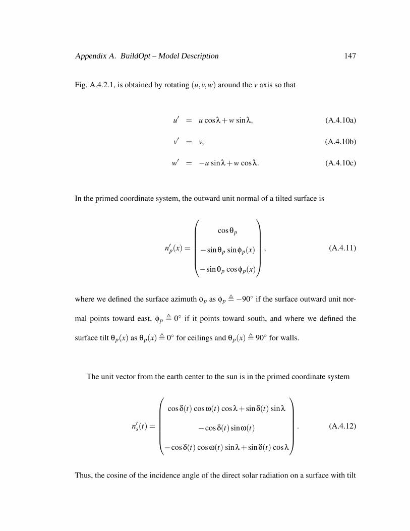
Appendix A. BuildOpt – Model Description 147
Fig. A.4.2.1, is obtained by rotating (u,v,w) around the v axis so that
u′ = u cosλ+w sinλ, (A.4.10a)
v′ = v, (A.4.10b)
w′ = −u sinλ+w cosλ. (A.4.10c)
In the primed coordinate system, the outward unit normal of a tilted surface is
n′p(x) =
cosθp
−sinθp sinφp(x)
−sinθp cosφp(x)
, (A.4.11)
where we defined the surface azimuth φp as φp ,−90 if the surface outward unit nor-
mal points toward east, φp , 0 if it points toward south, and where we defined the
surface tilt θp(x) as θp(x) , 0 for ceilings and θp(x) , 90 for walls.
The unit vector from the earth center to the sun is in the primed coordinate system
n′s(t) =
cosδ(t) cosω(t) cosλ+ sinδ(t) sinλ
−cosδ(t)sinω(t)
−cosδ(t) cosω(t) sinλ+ sinδ(t) cosλ
. (A.4.12)
Thus, the cosine of the incidence angle of the direct solar radiation on a surface with tilt

Appendix A. BuildOpt – Model Description 148
θp and azimuth φp(x) is
cosθi(x, t) = 〈n′p(x),n′s(t)〉
= cosθp(cosδ(t) cosω(t) cosλ+ sinδ(t) sinλ
)
+ sinθp sinφp(x) cosδ(t)sinω(t)
+ sinθp cosφp(x)(cosδ(t) cosω(t) sinλ− sinδ(t) cosλ
). (A.4.13)
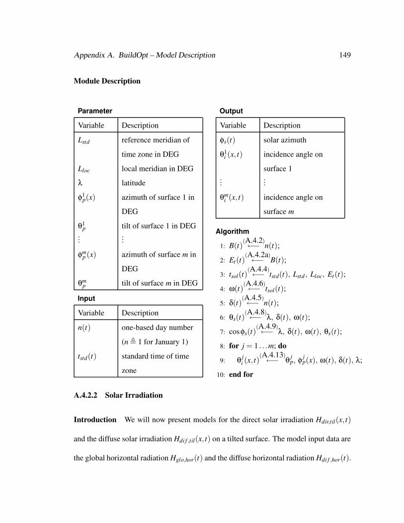
Appendix A. BuildOpt – Model Description 149
Module Description
Parameter
Variable Description
Lstd reference meridian of
time zone in DEG
Lloc local meridian in DEG
λ latitude
φ1p(x) azimuth of surface 1 in
DEG
θ1p tilt of surface 1 in DEG
......
φmp (x) azimuth of surface m in
DEG
θmp tilt of surface m in DEG
Input
Variable Description
n(t) one-based day number
(n , 1 for January 1)
tstd(t) standard time of time
zone
Output
Variable Description
φs(t) solar azimuth
θ1i (x, t) incidence angle on
surface 1...
...
θmi (x, t) incidence angle on
surface m
Algorithm
1: B(t)(A.4.2)←− n(t);
2: Et(t)(A.4.2a)←− B(t);
3: tsol(t)(A.4.4)←− tstd(t), Lstd , Lloc, Et(t);
4: ω(t)(A.4.6)←− tsol(t);
5: δ(t)(A.4.5)←− n(t);
6: θs(t)(A.4.8)←− λ, δ(t), ω(t);
7: cosφs(t)(A.4.9)←− λ, δ(t), ω(t), θs(t);
8: for j = 1 . . .m; do
9: θ ji (x, t)
(A.4.13)←− θ jp, φ j
p(x), ω(t), δ(t), λ;
10: end for
A.4.2.2 Solar Irradiation
Introduction We will now present models for the direct solar irradiation Hdir,til(x, t)
and the diffuse solar irradiation Hdi f ,til(x, t) on a tilted surface. The model input data are
the global horizontal radiation Hglo,hor(t) and the diffuse horizontal radiation Hdi f ,hor(t).
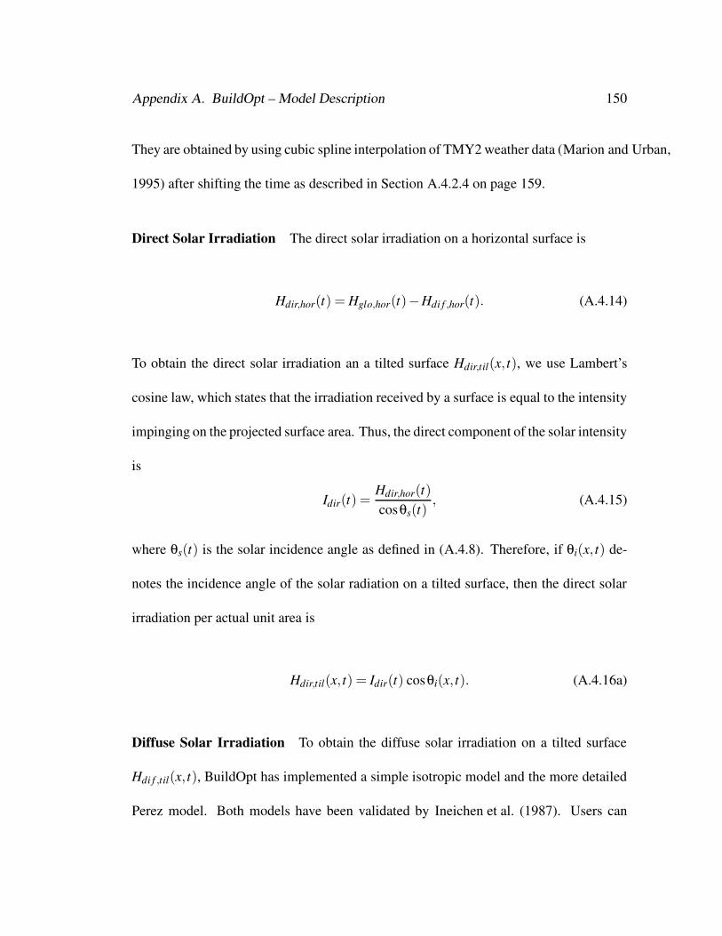
Appendix A. BuildOpt – Model Description 150
They are obtained by using cubic spline interpolation of TMY2 weather data (Marion and Urban,
1995) after shifting the time as described in Section A.4.2.4 on page 159.
Direct Solar Irradiation The direct solar irradiation on a horizontal surface is
Hdir,hor(t) = Hglo,hor(t)−Hdi f ,hor(t). (A.4.14)
To obtain the direct solar irradiation an a tilted surface Hdir,til(x, t), we use Lambert’s
cosine law, which states that the irradiation received by a surface is equal to the intensity
impinging on the projected surface area. Thus, the direct component of the solar intensity
is
Idir(t) =Hdir,hor(t)cosθs(t)
, (A.4.15)
where θs(t) is the solar incidence angle as defined in (A.4.8). Therefore, if θi(x, t) de-
notes the incidence angle of the solar radiation on a tilted surface, then the direct solar
irradiation per actual unit area is
Hdir,til(x, t) = Idir(t) cosθi(x, t). (A.4.16a)
Diffuse Solar Irradiation To obtain the diffuse solar irradiation on a tilted surface
Hdi f ,til(x, t), BuildOpt has implemented a simple isotropic model and the more detailed
Perez model. Both models have been validated by Ineichen et al. (1987). Users can
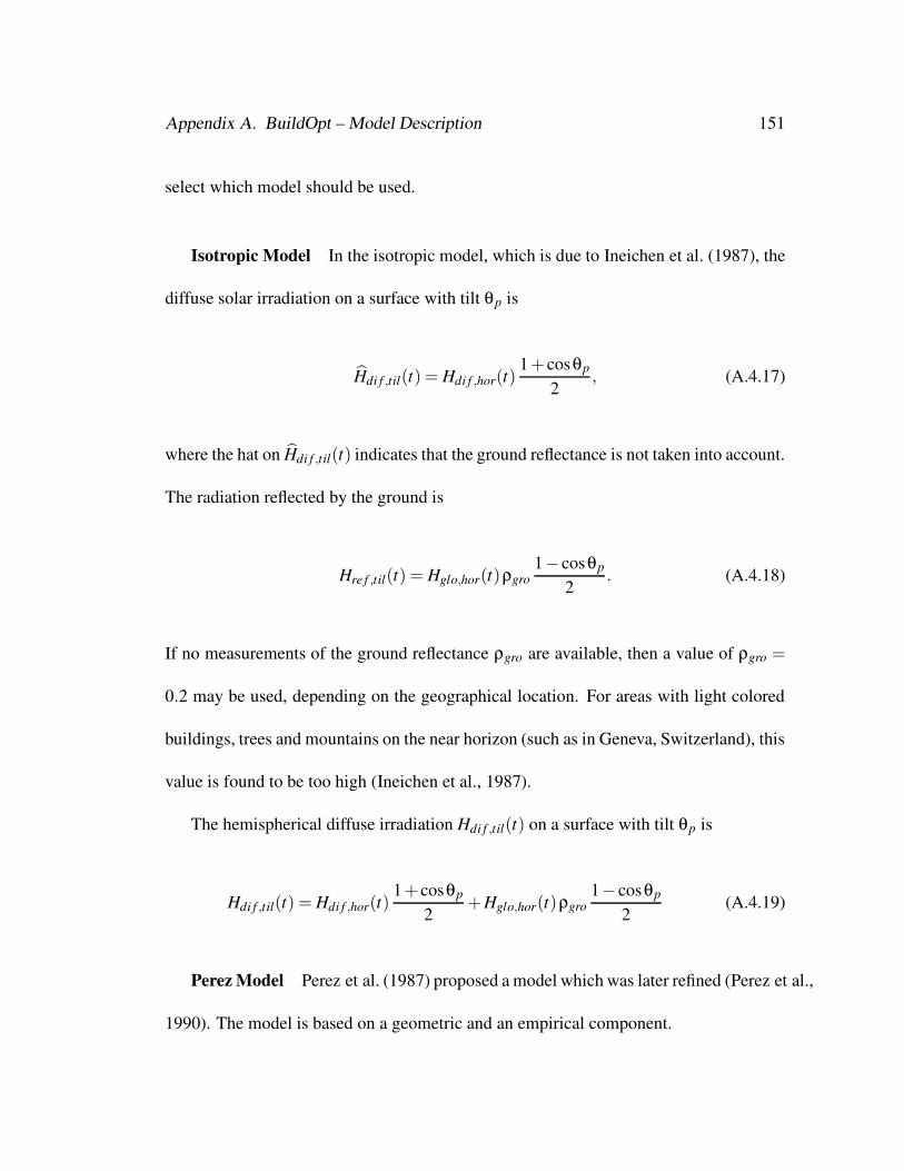
Appendix A. BuildOpt – Model Description 151
select which model should be used.
Isotropic Model In the isotropic model, which is due to Ineichen et al. (1987), the
diffuse solar irradiation on a surface with tilt θp is
Hdi f ,til(t) = Hdi f ,hor(t)1+ cosθp
2, (A.4.17)
where the hat on Hdi f ,til(t) indicates that the ground reflectance is not taken into account.
The radiation reflected by the ground is
Hre f ,til(t) = Hglo,hor(t)ρgro1− cosθp
2. (A.4.18)
If no measurements of the ground reflectance ρgro are available, then a value of ρgro =
0.2 may be used, depending on the geographical location. For areas with light colored
buildings, trees and mountains on the near horizon (such as in Geneva, Switzerland), this
value is found to be too high (Ineichen et al., 1987).
The hemispherical diffuse irradiation Hdi f ,til(t) on a surface with tilt θp is
Hdi f ,til(t) = Hdi f ,hor(t)1+ cosθp
2+Hglo,hor(t)ρgro
1− cosθp
2(A.4.19)
Perez Model Perez et al. (1987) proposed a model which was later refined (Perez et al.,
1990). The model is based on a geometric and an empirical component.

Appendix A. BuildOpt – Model Description 152
The geometric component describes the sky hemisphere using a circumsolar disk
and a horizon band that are superimposed on an isotropic background. This configu-
ration accounts for the most significant anisotropic effects in the atmosphere, namely
forward scattering by aerosols and multiple Rayleigh scattering and retro-scattering near
the horizon. The circumsolar brightening is assumed to originate from a point source
at the center of the sun. The horizon brightening is assumed to be a line source at the
horizon. In actuality, for clear skies, the horizon brightening is highest at the horizon and
decreases in intensity away from the horizon. For overcast skies the horizon brightening
has a negative value since the sky irradiation increases rather than decreases away from
the horizon.
The empirical component establishes the value of a circumsolar brightening coeffi-
cient F1 and a horizon brightening coefficient F2 as a function of the irradiation condi-
tions. F1 and F2 are parametrized by three quantities:
1. the position of the sun, defined by the zenith angle θs(t),
2. the brightness of the sky dome ∆(t), which is proportional to the horizontal diffuse
irradiation, and
3. the sky clearness ε(t), which is a function of the direct horizontal irradiation and
the diffuse horizontal irradiation.

Appendix A. BuildOpt – Model Description 153
The governing equation is
Hdi f ,til(x, t)Hdi f ,hor(t)
=
(1−F1(t)
)(1+ cosθp)
2+F1(t)
a(x, t)b(t)
+F2(t) sinθp. (A.4.20)
The coefficients F1(·) and F2(·) are obtained empirically from experimental data
recorded on sloping surfaces. To compute F1(t) and F2(t), we first need to obtain an
expression for the sky brightness, which depends on the relative air mass, and for the
sky clearness. The relative air mass is (Perez, 1999)
mair(t) =1
cos(θs(t)
)+0.15
(93.9−θs(t)
)−1.253 , mair=−, θs= DEG.
(A.4.21)
The sky brightness ∆(t), with 0≤ ∆(t)≤ 1, is defined in Perez et al. (1990) as
∆(t) , Hdi f ,hor(t)mair(t)
I0, ∆=−, (A.4.22)
where I0 = 1367.0W/m2 is the extraterrestrial radiation. If θs(t) is close to 90 , then
∆(t) can be larger than unity, which can cause the diffuse radiation to be larger than the
solar constant. To prevent this, we reformulate (A.4.22) as
∆(t) , min(
Hdi f ,hor(t)mair(t)
I0,1; 0.025
), ∆=−. (A.4.23)
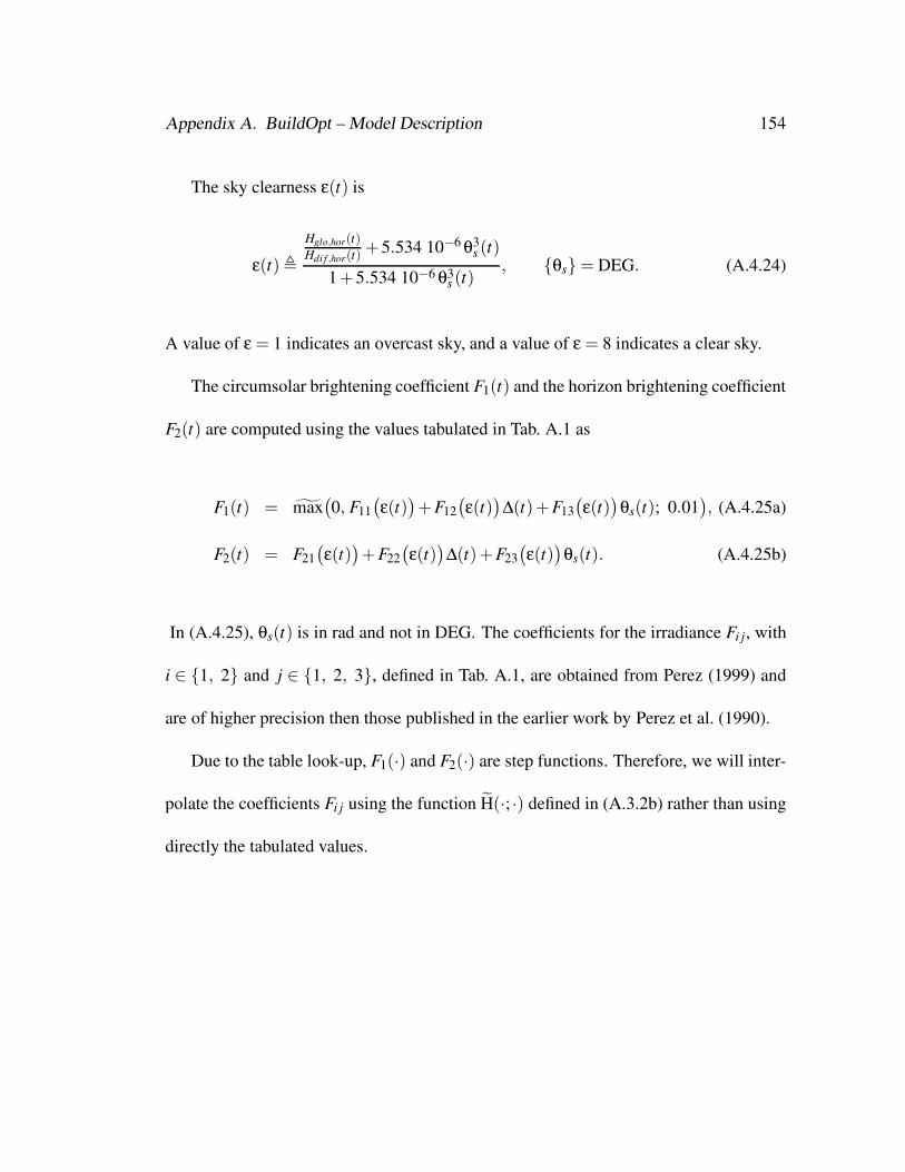
Appendix A. BuildOpt – Model Description 154
The sky clearness ε(t) is
ε(t) ,
Hglo,hor(t)Hdi f ,hor(t)
+5.534 10−6 θ3s (t)
1+5.534 10−6 θ3s (t)
, θs= DEG. (A.4.24)
A value of ε = 1 indicates an overcast sky, and a value of ε = 8 indicates a clear sky.
The circumsolar brightening coefficient F1(t) and the horizon brightening coefficient
F2(t) are computed using the values tabulated in Tab. A.1 as
F1(t) = max(0, F11
(ε(t))+F12
(ε(t))
∆(t)+F13(ε(t))
θs(t); 0.01), (A.4.25a)
F2(t) = F21(ε(t))+F22
(ε(t))
∆(t)+F23(ε(t))
θs(t). (A.4.25b)
In (A.4.25), θs(t) is in rad and not in DEG. The coefficients for the irradiance Fi j, with
i ∈ 1, 2 and j ∈ 1, 2, 3, defined in Tab. A.1, are obtained from Perez (1999) and
are of higher precision then those published in the earlier work by Perez et al. (1990).
Due to the table look-up, F1(·) and F2(·) are step functions. Therefore, we will inter-
polate the coefficients Fi j using the function H(·; ·) defined in (A.3.2b) rather than using
directly the tabulated values.

Appendix
A.
BuildO
pt–M
odelDescription
155
ε bin F11 F12 F13 F21 F22 F23ε≤ 1.065 −0.0083117 0.5877285 −0.0620636 −0.0596012 0.0721249 −0.0220216
1.065 < ε≤ 1.23 0.1299457 0.6825954 −0.1513725 −0.0189325 0.0659650 −0.02887481.23 < ε≤ 1.50 0.3296958 0.4868735 −0.2210958 0.0554140 −0.0639588 −0.02605421.50 < ε≤ 1.95 0.5682053 0.1874525 −0.2951290 0.1088631 −0.1519229 −0.01397541.95 < ε≤ 2.80 0.8730280 −0.3920403 −0.3616149 0.2255647 −0.4620442 0.00124482.80 < ε≤ 4.50 1.1326077 −1.2367284 −0.4118494 0.2877813 −0.8230357 0.05586514.50 < ε≤ 6.20 1.0601591 −1.5999137 −0.3589221 0.2642124 −1.1272340 0.13106946.20 < ε 0.6777470 −0.3272588 −0.2504286 0.1561313 −1.3765031 0.2506212
Table A.1: Perez model coefficients for irradiance.

Appendix A. BuildOpt – Model Description 156
In (A.4.20), the term F1 a/b accounts for the circumsolar region, with
a(x, t) = max(0, cosθi(x, t); 0.01), (A.4.26a)
b(t) = max(cos85, cosθs(t); 0.01). (A.4.26b)
Adding the radiation reflected by the ground, as defined in (A.4.18) to (A.4.20), yields
the hemispherical diffuse irradiation Hdi f ,til(x, t) on a surface with tilt θp as
Hdi f ,til(x, t) = Hdi f ,hor(t)
(1−F1(t)
)(1+ cosθp)
2+F1(t)
a(x, t)b(t)
+F2(t) sinθp
+Hglo,hor(t)ρgro1− cosθp
2. (A.4.27)

Appendix A. BuildOpt – Model Description 157
Module Description
Parameter
Variable Description
nm number of model (1 =
isotropic; 2 = Perez)
ρgro ground reflectance,
ρgro ∈ [0, 1]
θ1p tilt of surface 1 in DEG
......
θmp tilt of surface m in DEG
Input
Variable Description
Hglo,hor(t) global horizontal
irradiation per unit area
Hdi f ,hor(t) diffuse horizontal
irradiation per unit area
θs(t) solar zenith in DEG
θ1i (x, t) solar incidence angle on
surface 1 in DEG...
...
θmi (x, t) solar incidence angle on
surface m in DEG
Output
Variable Description
H1dir,til(x, t) direct solar irradiation
on surface 1
H1di f ,til(x, t) diffuse solar irradiation
on surface 1...
...
Hmdir,til(x, t) direct solar irradiation
on surface m
Hmdi f ,til(x, t) diffuse solar irradiation
on surface m

Appendix A. BuildOpt – Model Description 158
Algorithm
1: Direct irradiation2: Hdir,hor(t)
(A.4.14)←− Hglo,hor(t), Hdi f ,hor(t);
3: for j=1 . . . m do
4: H jdir,til(x, t)
(A.4.16a)←− Hdir,hor(t), θ ji (x, t), θs(t);
5: end for
6: Diffuse irradiation7: if nm = 1 then
8: Model 1: Isotropic9: for j=1 . . . m do
10: H jdi f ,til(t)
(A.4.19)←− Hdi f ,hor(t), Hglo,hor(t), θ jp, ρgro;
11: end for
12: else
13: Model 2: Perez14: mair(t)
(A.4.21)←− θs(t);
15: ∆(t)(A.4.23)←− Hdi f ,hor(t), mair(t);
16: ε(t)(A.4.24)←− Hdir,hor(t), Hdi f ,hor(t), θs(t);
17: F1,i3i=1(t)←− ε(t); (see Tab. A.1)
18: F2,i3i=1(t)←− ε(t); (see Tab. A.1)
19: F1(t)(A.4.25a)←− F1, j3
j=1(t), ∆(t), θs(t);
20: F2(t)(A.4.25b)←− F2, j3
j=1(t), ∆(t), θs(t);
21: b(t)(A.4.26b)←− θs(t);
22: for j=1 . . . m do
23: a(x, t)(A.4.26a)←− θ j
i (x, t);
24: H jdi f ,til(x, t)
(A.4.27)←− Hdi f ,hor(t), Hglo,hor(t), F1(t), F2(t), θ jp, ρgro, a(x, t), b(t);
25: end for
26: end if

Appendix A. BuildOpt – Model Description 159
A.4.2.3 Air Density
The air density as a function of the altitude is
ρair(h) = ρair,0 exp(a/h) , (A.4.28)
where h is the elevation in meters, ρair,0 = 1.201kg/m3 is the air density at sea level and
a =−1.21975510−4 m−1 (see Judkoff and Neymark (1995)).
A.4.2.4 Weather Data
We use the Typical Meteorological Year 2 (TMY2) weather data set to obtain hourly
weather data (Marion and Urban, 1995). The TMY2 weather data are based on solar
time, which we compute using equation (A.4.4).
In the TMY2 weather data set, the recorded hourly solar radiation data are defined
as the amount of radiative energy received during the solar hour ending at the hour indi-
cated in the weather data file. Due to recording values that have been integrated over the
last 60 minutes, the recorded radiation data have an average time delay of 30 minutes.
Due to this time delay, the data set lists some hours where the direct solar radiation is
nonzero but the sun is already behind the horizon. To reduce this problem and to increase
the accuracy, we use solar data that were recorded 30 minutes in the future of the current
solar time.

Appendix A. BuildOpt – Model Description 160
We interpolate all weather data using cubic spline interpolation (Press et al., 1992).
For time stamps at which weather data are missing, the values of the last recorded hour
are used.
A.4.2.5 Sky Temperature
Model To obtain an expression for the long-wave radiative heat exchange between the
building and the possibly cloudy sky, we use the sky model from Martin and Berdahl
(1984). Martin and Berdahl use weather data that are recorded in the Typical Meteo-
rological Year (TMY) weather data (NCDC, 1981). Since we use TMY2 weather data
which are different from TMY weather data, we have to slightly modify the computation
of the infrared cloud amount C(t).
To obtain the long-wave radiative heat exchange between a surface at ground level
and the sky, the model computes a so-called black-body sky temperature Tsky(t).
We will first obtain the clear sky emissivity εclear(t). Martin and Berdahl describe an
emissivity ε0(t) as a function of the dew point temperature Td p(t) as
ε0(t) = 0.711+0.56(
Td p(t)100
)+0.73
(Td p(t)100
)2
, Td p= C. (A.4.29)

Appendix A. BuildOpt – Model Description 161
They also describe a diurnal correction which takes different observed sky emissivities
at day and night into account (Berdahl and Fromberg, 1982; Berdahl and Martin, 1984;
Martin and Berdahl, 1984). The diurnal correction is
∆εh(t) = 0.013 cos(
2πtsol(t)
24
), (A.4.30)
where tsol(t) is the solar time introduced in (A.4.4).
An elevation correction, takes the elevation of the observing weather station into
account. The elevation correction is
∆εe(t) = 0.00012(P(t)−1000
), P= mbar, (A.4.31)
where P(t) is the air pressure at the station.
The clear sky emissivity εclear(t) is the sum of ε0(t), the diurnal correction ∆εh(t)
and the elevation correction ∆εe(t):
εclear(t) = ε0(t)+∆εh(t)+∆εe(t). (A.4.32)
The presence of clouds is taken into account by introducing an infrared cloud amount
C(t), defined as
C(t) ,ε(t)− εclear(t)
1− εclear(t), (A.4.33)

Appendix A. BuildOpt – Model Description 162
where ε(t) is the cloudy sky emissivity.
The infrared cloud amount C(t) can also be expressed as
C(t) = n(t)εc(t)Γ(t), (A.4.34)
where n(t) is the fractional area of the sky that is covered by clouds, εc(t) is the hemi-
spherical cloud emissivity, and Γ(t) is a factor that depends on the cloud base tempera-
ture. The factor Γ(t) is small for high (cold) clouds and approaches unity for low clouds.
Since usually no data for the cloud base temperature are available, Martin and Berdahl
approximated Γ(t) as a function of the cloud base height using the expression
Γ(t) = exp(
h(t)h0
), (A.4.35)
where h(t) is the cloud base height and h0 , 8.2km.
For multiple cloud layers, Martin and Berdahl added (A.4.34) for each cloud layer.
However, the TMY2 weather data set contains only hourly information of (i) the total
sky cover3 nto(t), (ii) the opaque sky cover4 nop(t), and (iii) the ceiling height h. Hence,
we will obtain the sky cover due to high clouds from the total and the opaque sky cover.
We assume that high clouds are thin clouds, such as cirrus clouds, and hence, compute
3The total sky cover is defined as the amount of the sky dome in tenths covered by clouds or obscuringphenomena (Marion and Urban, 1995).
4The opaque sky cover is defined as the amount of the sky dome in tenths covered by clouds or ob-scuring phenomena that prevents observing the sky or higher cloud layers (Marion and Urban, 1995).
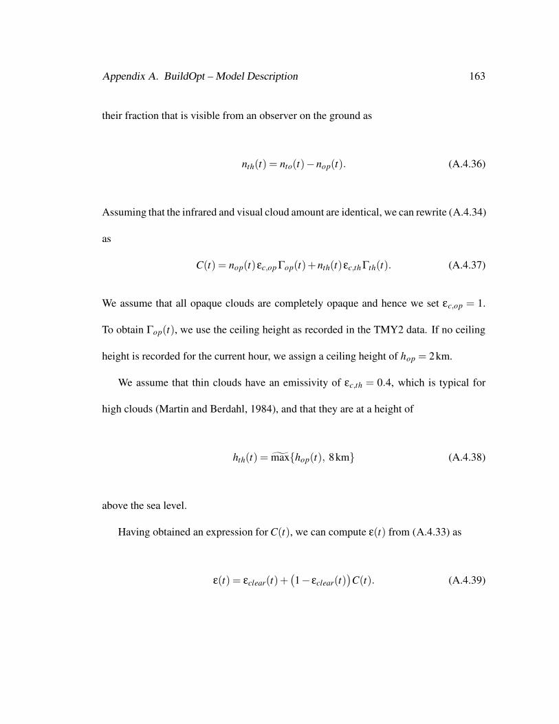
Appendix A. BuildOpt – Model Description 163
their fraction that is visible from an observer on the ground as
nth(t) = nto(t)−nop(t). (A.4.36)
Assuming that the infrared and visual cloud amount are identical, we can rewrite (A.4.34)
as
C(t) = nop(t)εc,op Γop(t)+nth(t)εc,th Γth(t). (A.4.37)
We assume that all opaque clouds are completely opaque and hence we set εc,op = 1.
To obtain Γop(t), we use the ceiling height as recorded in the TMY2 data. If no ceiling
height is recorded for the current hour, we assign a ceiling height of hop = 2km.
We assume that thin clouds have an emissivity of εc,th = 0.4, which is typical for
high clouds (Martin and Berdahl, 1984), and that they are at a height of
hth(t) = maxhop(t), 8km (A.4.38)
above the sea level.
Having obtained an expression for C(t), we can compute ε(t) from (A.4.33) as
ε(t) = εclear(t)+(1− εclear(t)
)C(t). (A.4.39)

Appendix A. BuildOpt – Model Description 164
Finally, the black-body sky temperature can be computed as
Tsky(t) = ε(t)1/4 Tdb(t), (A.4.40)
where Tdb(t) is the dry bulb temperature at ground level.

Appendix A. BuildOpt – Model Description 165
Module Description
Parameter
Variable Description
none
Input
Variable Description
tsol(t) solar time, as defined in
(A.4.4)
Tdb(t) dry bulb temperature
(from TMY2)
Td p(t) dew point temperature
(from TMY2)
nto total sky cover (nto(t) ∈0, 1, . . . ,10, from
TMY2)
nop opaque sky cover
(nop(t) ∈0, 1, . . . ,10, from
TMY2)
hop(t) ceiling height (from
TMY2)
P(t) atmospheric pressure at
weather station (from
TMY2)
Output
Variable Description
Tsky(t) black body sky
temperature
ε(t) cloudy sky emissivity
Algorithm
1: hth(t)(A.4.38)←− hop(t);
2: Γop(t)(A.4.35)←− hop(t);
3: Γth(t)(A.4.35)←− hth(t);
4: nth(t)(A.4.36)←− nto(t), nop(t);
5: C(t)(A.4.37)←− nop(t), nth(t), Γop(t), Γth(t),
εc,op, εc,th;
6: ε0(t)(A.4.29)←− Td p(t);
7: ∆εh(t)(A.4.30)←− tsol(t);
8: ∆εe(t)(A.4.31)←− P(t);
9: εclear(t)(A.4.32)←− ε0(t), ∆εh(t), ∆εe(t);
10: ε(t)(A.4.39)←− εclear(t), C(t);
11: Tsky(t)(A.4.40)←− ε(t), Tdb(t);

Appendix A. BuildOpt – Model Description 166
A.4.2.6 Heat Gains
Solar Gains To compute the solar gains per unit area for the room surfaces, we assume
that all solar radiation that enters the room first hits the floor, and that the floor diffusely
reflects the radiation to all other surfaces. We neglect multiple reflections and instead of
using view factors between the floor and the other surfaces, we use area weighted solar
distribution factors. The model is as follows:
Consider a room with N f floor patches. Let N f be the set of indices of all floor
area patches and let H(x, t) denote the solar radiation transmitted from the outside to the
room. The solar radiation that is absorbed by the k-th floor patch per unit area is
qk(x, t) = H(x, t)εk
sol
∑n∈N f An(x). (A.4.41a)
The solar radiation that is reflected from the k-th floor patch is
Qkr(x, t) = H(x, t)
Ak(x)(1− εksol)
∑n∈N f An(x). (A.4.41b)
Therefore, the solar radiation that is reflected by the whole floor area is
Qr(x, t) = ∑n∈N f
Qnr (x, t) = H(x, t)
∑n∈N fAn(x)(1− εn
sol)
∑n∈N f An(x). (A.4.41c)
We distribute Qr(x, t) to all non-floor areas, weighted by their solar absorptivity εsol and
solar transmissivity for diffuse irradiation τsol (which is non-zero for windows). Let M

Appendix A. BuildOpt – Model Description 167
be the index set of all non-floor surface patches. We compute the solar radiation that is
absorbed or transmitted by a non-floor surface patch per unit area as
qk(x, t) = Qr(x, t)εk
sol + τksol
∑m∈M Am(x)(εmsol + τm
sol). (A.4.41d)
For opaque constructions, qk(x, t) is assumed to be completely absorbed. For windows,
however, part of qk(x, t) is transmitted to the outside, and only a fraction of qk(x, t) is
absorbed. Thus, we consider qk(x, t) as the solar radiation that hits the window from the
room-side. What fraction of qk(x, t) will be absorbed by each window pane is determined
in the window model (see Section A.4.3.3 on page 189).
Internal Gains The heat gains caused by appliances, such as computers, and by people
are defined by hourly, weekly, and yearly schedules. The schedules can be defined as
discrete, continuous or differentiable schedules, and it can be specified what fraction of
the energy is radiative and what fraction is convective.
1. Discrete schedules do not use interpolation to obtain values at intermediate time
steps. For discrete schedules, if ti and ti+1 have schedule values si and si+1, we
assign for t ∈ [ti, ti+1) the value s(t) = si.
2. Continuous schedules use linear interpolation to obtain values at intermediate time
steps. If ti and ti+1 have schedule values si and si+1, we assign for t ∈ [ti, ti+1) the
value s(t) = si +(si+1− si)t−ti
ti+1−ti.

Appendix A. BuildOpt – Model Description 168
3. Differentiable schedules use interpolation based on the once Lipschitz continu-
ously differentiable Heaviside function, defined in (A.3.2b), to obtain values at
intermediate time steps. If ti and ti+1 have schedule values si and si+1, we assign
for t ∈ [ti, ti+1) the value
s(t) = si +(si+1− si) H(
t− ti−ti+1− ti
2;ti+1− ti
2
). (A.4.41e)
This defines a once Lipschitz continuously differentiable schedule, which signif-
icantly improves the convergence properties of the DASPK solver that is used to
solve the system of differential algebraic equations.
For radiative internal gains, the i-th surface is assumed to absorb the heat gain per
unit area
H iIR(t) =
εiIR
∑Nsurn=1 εn
IR An(x)P(t), (A.4.41f)
where Ai(x) denotes the area of the i-th surface, with i∈ 1, . . . ,Nsur, εiIR denotes the ab-
sorptivity of the i-th surface for infrared radiation, and P(t) denotes the radiative internal
heat gain of the zone.

Appendix A. BuildOpt – Model Description 169
A.4.3 Heat Transfer in the Building
We will now present the models that describe the heat transfer processes in the build-
ing.
A.4.3.1 Surface Heat Transfer
Introduction We will now present a simplified and a detailed model for the convective
heat transfer coefficient hcon(x, t). For exterior surfaces, the convective heat transfer co-
efficient hcon(x, t) accounts for buoyancy driven free convection h f re(x, t) and for forced
convection caused by wind h f or(x, t). We define
hcon(x, t) , h f re(x, t)+h f or(x, t). (A.4.42)
For the design of thermal storage elements, such as concrete interior walls, the accurate
computation of the room-side heat transfer coefficient is important since it couples the
room air temperature to the storage element. Therefore, we give the user the option to
select either a simplified or a detailed heat transfer model for the interior surfaces, but
we always use a simplified model for the exterior surfaces.
We will also present an equation for the radiative heat transfer coefficient that is
used to compute the radiative heat transfer between exterior surfaces and the sky and the
ground.

Appendix A. BuildOpt – Model Description 170
Simplified Model
Convective Heat Transfer Coefficient for Free Convection For the simplified
model, we will use constant convective heat transfer coefficients. EnergyPlus 1.1.0 uses
for the simplified method convective heat transfer coefficients that were obtained from
a correlation from Fig. 1 on page 22.4 in the ASHRAE Handbook of Fundamentals
(ASHRAE, 1989). The values used in EnergyPlus are:
• For horizontal surfaces, i.e., surfaces with tilt θp ∈ (−22.5, 22.5):
h f re(x, t) =
0.948W/(m2 K), for reduced convection,
4.040W/(m2 K), for enhanced convection.
(A.4.43a)
• For tilted surfaces:
h f re(x, t) =
2.281W/(m2 K), for reduced convection,
3.076W/(m2 K), for vertical surface,
3.870W/(m2 K), for enhanced convection.
(A.4.43b)
Reduced convection means that the heat flux is opposite to the buoyancy force, and en-
hanced convection means that the heat flux is in the same direction as the buoyancy
force. Since the direction of the heat flux depends on the design parameter x, the equa-
tions above are discontinuous in x. Therefore, we will further simplify the model and

Appendix A. BuildOpt – Model Description 171
use for any surface and any heat flux h f re = 3W/(m2 K).
Convective Heat Transfer Coefficient for Forced Convection To take an in-
crease in the convective heat transfer coefficient due to wind into account, we use in
the simplified model h f or = h f re.
Radiative Heat Transfer at Exterior Surfaces To calculate infrared radiation be-
tween the exterior building surface and the outside environment, we treat the environ-
ment as an enclosure with much larger area than the building surface. Then, the heat
exchange is
qIR(x, t) = σεIR (T 4env(t)−T 4
sur(x, t)), (A.4.44a)
where Tenv(·) denotes the environment temperature and Tsur(·, ·) denotes the surface tem-
perature of the building construction element for which the heat transfer is computed.
Let Fsur−gro denote the view factor from the surface to the ground. We define the
environment temperature as
Tenv(t) , 4√
Fsur−gro T 4out(t)− (1−Fsur−gro)T 4
sky(t), (A.4.44b)
where Tout(t) is the outside air temperature, and Tsky(t) is the sky temperature defined
in (A.4.40). For equation (A.4.44b), we assumed that the ground temperature is equal to
the air temperature.

Appendix A. BuildOpt – Model Description 172
We linearize (A.4.44a) to obtain
qIR(x, t) = 4σεIR T 3env(t)(Tenv(t)−Tsur(x, t)). (A.4.44c)
Thus, we can define a radiative heat transfer coefficient as
hIR(t) = 4σεIR T 3env(t). (A.4.44d)
Radiative Heat Transfer To compute the radiative heat transfer between the room
surfaces, we define a radiation temperature T ∗(x, t) as
T ∗(x, t) ,∑Nsur
n=1 εnIR An(x)T n
sur(x, t)
∑Nsurn=1 εn
IR An(x). (A.4.45a)
We assume that each surface only exchanges radiation with an imaginary surface of
much larger area which is at temperature T ∗(x, t). By using a linearized heat transfer
coefficient, defined as
hnIR(x, t) , 4σεn
IR T ∗(x, t)3, (A.4.45b)
we can write
qnIR(x, t) = hn
IR(x, t)(T ∗(x, t)−T n(x, t)
). (A.4.45c)

Appendix A. BuildOpt – Model Description 173
Equations (A.4.45c) and (A.4.45a) are consistent with conservation of energy because
Nsur
∑n=1
An qnIR(x, t) = 4σ
(T ∗(x, t)
)3Nsur
∑n=1
εnIR An (T ∗(x, t)−T n(x, t)
)
= 4σ(T ∗(x, t)
)3
(Nsur
∑n=1
εnIR An T ∗(x, t)−
Nsur
∑n=1
εnIR An T n(x, t)
)
= 0. (A.4.45d)
Detailed Model We will now present the detailed model which the user can select for
computing the room-side heat transfer coefficient.
Convective Heat Transfer Coefficient for Free Convection In the detailed model,
the convective heat transfer coefficient for free convection h f re(x, t) is for each sur-
face computed as a function of the temperature difference (T∞(x, t)− Tsur(x, t)), with
T∞(x, t) , Tair(x, t) for interior surfaces and T∞(x, t) , Tout(t) for exterior surfaces. We
use the once Lipschitz continuously differentiable equation
h f re(x, t) = max(1, h f re(x, t); 0.1), (A.4.46a)

Appendix A. BuildOpt – Model Description 174
where
h f re(x, t) =
1.310∣∣T∞(x, t)−Tsur(x, t)
∣∣1/3, for vert. surface,
1.510∣∣T∞(x, t)−Tsur(x, t)
∣∣1/3, for horiz. surf., enhanced conv.,
0.760∣∣T∞(x, t)−Tsur(x, t)
∣∣1/3, for horiz. surf., reduced conv.
(A.4.46b)
Enhanced convection means that the heat flux is in the same direction as the buoyancy
force, and reduced convection in the other direction. We smoothen the computation
by using (A.4.46a) rather than only (A.4.46b) because the convective heat transfer, if
computed as q(x, t) = c(T∞(x, t)− Tsur(x, t)
)∣∣T∞(x, t)− Tsur(x, t)∣∣1/3, for some c 6= 0,
is not Lipschitz continuously differentiable in the temperature difference as |T∞(x, t)−
Tsur(x, t)| → 0.
Note that we described the convective heat transfer coefficient as a function of the
temperature difference only. More detailed correlations that account for the increased
air velocity near the room surfaces when the HVAC system is running can be found in
Clarke (2001), but they are not implemented in the current version of BuildOpt.
Radiative Heat Transfer for Interior Surfaces In the detailed model, the radiative
heat transfer for interior surfaces is computed as in the simplified model.

Appendix A. BuildOpt – Model Description 175
Module Description For Convective Heat Transfer Coefficients
Parameter
Variable Description
θp surface tilt in DEG (0
for floor; ±90 for wall;
180 for ceiling)
For exterior surfaces only:
nm number of model (1 =
simplified model; 2 =
detailed model)
εIR infrared emissivity
Fsur−gro view factor from
surface to ground
Input
Variable Description
Tsur(x, t) surface temperature
T∞(x, t) air temperature (Tout(t)
or Tair(x, t))
For exterior surfaces only:
Tsky(t) sky temperature as
defined in (A.4.40)
Output
Variable Description
hcon(x, t) convective heat transfer
coefficient
A.4.3.2 Heat Conductance in Opaque Material
We will now describe how the heat conductance through walls, ceilings and floors is
computed.
Governing Equation The one-dimensional heat conductance in composite construc-
tions that are composed of layers of opaque materials can be described by
∂∂z
(k(z)
∂T (x;z, t)∂z
)= C(z)
∂T (x;z, t)∂t
, (A.4.47a)

Appendix A. BuildOpt – Model Description 176
for (z, t)∈Ω×(0, τ), for some τ > 0, where Ω ,(0 , l)
and l > 0 denotes the construction
length and T (x; ·, ·) denotes the construction temperature. We make the convention that
the room-side surface is at z = 0 and that the outside surface is at z = l. The coefficients
k,C : R→R are piece-wise constant functions for the heat conductivity and the specific
heat capacity per unit volume, respectively. We use the initial data
T (x;z,0) = η(x;z), z ∈Ω, (A.4.47b)
where η(x; ·) is continuous, and we use the boundary conditions, for t ∈ (0, τ),
k(0)∂T (x;0, t)
∂z−h0(x; t)T (x;0, t) = g0(x; t), (A.4.47c)
−k(l)∂T (x; l, t)
∂z−h1(x; t)T (x; l, t) = g1(x; t), (A.4.47d)
where h0(x; ·), h1(x; ·), g0(x; ·), and g1(x; ·) are once Lipschitz continuously differen-
tiable functions if the weather data and the internal heat gains are interpolated using
a once Lipschitz continuously differentiable function (see Section A.4.2.4 and Sec-
tion A.4.2.6). They are defined as
h0(x; t) , hcon,0(x; t)+hlw,0(x; t) (A.4.48a)
h1(x; t) , hcom,1(x; t)+hlw,1(x; t) (A.4.48b)

Appendix A. BuildOpt – Model Description 177
where hcon,0(x, ·) is the room-side convective heat transfer coefficient, hlw,0(x, ·) is the
room-side radiative heat transfer coefficient, hcon,1(x, ·) is the outside convective heat
transfer coefficient, and hlw,1(x, ·) is the outside radiative heat transfer coefficient, all
defined in Section A.4.3.1 on page 169.
The functions g0(x; ·) and g1(x; ·) are defined as
g0(x; t) , −hcon,0(t)T∞,0(x; t)−hlw,0(x; t)Tenv,0(x; t)−g′′0(x; t), (A.4.49a)
g1(x; t) , −hcon,1(t)T∞,l(x; t)−hlw,1(x; t)Tenv,1(x; t)−g′′1(x; t), (A.4.49b)
where T∞,0(x; ·) and T∞,1(x; ·) are the air temperatures outside the thermal boundary layer,
Tenv,0(x; ·) is the radiation temperature introduced in (A.4.45a), Tenv,1(x; ·) is for exterior
constructions the environment temperature introduced in (A.4.44b) and for interior con-
struction the room radiation temperature T ∗(x, t) introduced in (A.4.45a) of the adjacent
zone, and g′′0(x; ·) and g′′1(x; ·) are the short wave radiative heat gains of the surface due
to solar radiation or due to radiative internal heat gains caused by appliances, such as
lights and computers, which are once Lipschitz continuously differentiable functions
if the weather data and the internal heat gains are interpolated using a once Lipschitz
continuously differentiable function (see Section A.4.2.4 and Section A.4.2.6).
By introducing the notations
Tt(x;z, t) ,∂T (x;z, t)
∂t, Tz(x;z, t) ,
∂T (x;z, t)∂z
, (A.4.50a)

Appendix A. BuildOpt – Model Description 178
and the second order differential operator
L(·) ,− ∂∂z
(k(z)
∂(·)∂z
), (A.4.50b)
equation (A.4.47) can be formulated in the more concise form, for z ∈Ω and t ∈ (0, τ),
C(z)Tt(x;z, t)+LT(x;z, t) = 0, (A.4.51a)
T (x;z,0) = η(x;z), (A.4.51b)
k(0)Tz(x;0, t)−h0(t)T(x;0, t) = g0(x; t), (A.4.51c)
−k(l)Tz(x; l, t)−h1(t)T(x; l, t) = g1(x; t). (A.4.51d)
In composite walls, the material properties of adjacent layers, say in material 1 and
material 2, can be so that k1/k2 ≈ 10−1, C1/C2 ≈ 102, and hence the ratio of the thermal
diffusivities α , k/C can be α1/α2 ≈ 101. Thus, the thermal diffusivity in adjacent
layers can vary by an order of magnitude. Because the coefficients k(·) and C(·) are
discontinuous, there is no function u(x; ·, ·) that is two times continuously differentiable
in z at the material interfaces and that satisfies (A.4.51). Thus, equation (A.4.51) does
not have a classical solution, and we therefore seek a weak solution using the Galerkin
method.
Galerkin Approximations In the Galerkin method (Evans, 1998; Strang and Fix, 1973),
one builds a weak solution of (A.4.51) by first constructing solutions of certain finite-

Appendix A. BuildOpt – Model Description 179
dimensional approximations to (A.4.51) and then passing to limits. We will use contin-
uous, piece-wise linear functions to approximate a weak solution of (A.4.51). We will
now explain our implementation.
For j ∈ 1, 2, . . ., let φ j : Ω(·)→ R be piece-wise linear hat functions, which we
will call test functions, and which are defined for 0 ≤ z j−1 < z j < z j+1 ≤ l and for all
z ∈ (0, l) by
φ j(z) ,
z−z j−1z j−z j−1
, if z ∈[z j−1,z j
),
z−z j+1z j−z j+1
, if z ∈[z j,z j+1
),
0, otherwise.
(A.4.52)
For a fixed positive integer N, we construct an approximate solution TN(x; ·, ·) of the
form
TN(x;z, t) =N
∑j=1
γ jN(x; t)φ j(z), (A.4.53)
where the coefficients γ jN(x; ·)N
j=1 are so that
γ jN(x;0) =
Ω
η(x;z)φ j(z)dz, j ∈ 1, . . . ,N, (A.4.54a)

Appendix A. BuildOpt – Model Description 180
zΩk−1 Ωk
γk−1N (x; t)φk−1(z) γk
N(x; t)φk(z)
γk+1N (x; t)φk+1(z)
TN(x;z, t)
zk−1 zk zk+1
Figure A.6: Approximate solution constructed by the Galerkin method.
and
Ω
(C(z)
∂TN(x;z, t)∂t
+LTN(x;z, t))
φ j(z)ds = 0, t ∈ (0, τ), j ∈ 1, . . . ,N.
(A.4.54b)
Fig. A.6 shows an example of an approximate solution TN(x; ·, ·) constructed using piece-
wise linear hat functions.
Construction of Test Functions An expression for the coefficients γ jN(x; ·)N
j=1 is
obtained by substituting (A.4.53) into (A.4.54b). Using integration by parts, we obtain,

Appendix A. BuildOpt – Model Description 181
for k ∈ 1, . . . ,N,
0 =N
∑j=1
Ω
C(z)dγ j
N(x; t)dt
φ j(z)φk(z)+ γ jN(x; t)L
(φ j(z)
)φk(z)dz
=N
∑j=1
(dγ j
N(x; t)dt
Ω
C(z)φ j(z)φk(z)dz+ γ jN(x; t)
Ω
k(z)dφ j(z)
dzdφk(z)
dzdz
)
− k(z)dTN(x;z)
dzφk(z)
∣∣∣∣l
z=0. (A.4.55)
We now divide the domain Ω into N − 1 subdomains Ω j ,(z j,z j+1
), with j ∈
1, . . . ,N− 1, which we will call elements. The locations of the support points z j are
so that each point of discontinuity of k(·) and C(·) coincides with some z j.
The integrals in (A.4.55) are zero except for j = k− 1, for j = k, and for j = k + 1.
Since the elements Ω j differ from each other only in a scaling factor, it is convenient to
evaluate the different components of (A.4.55) on a so-called master element, which is
indicated by a superscript “M” and which is shown in Fig. A.7.
In terms of the master element, the integrals in (A.4.55) have the solutions
ΩM
φM1 (z)φM
2 (z)dz =
zM2
zM1
z− zM1
zM2 − zM
1
zM2 − z
zM2 − zM
1dz =
zM2 − zM
16
, (A.4.56a) ΩM
(φM
1 (z))2
dz =
ΩM
(φM
2 (z))2
dz =zM
2 − zM1
3, (A.4.56b)

Appendix A. BuildOpt – Model Description 182
1
ΩM
φM1 (z) φM
2 (z)
zM1 zM
2
Figure A.7: Master element with master basis functions.
and
ΩM
dφM1 (z)dz
dφM2 (z)dz
dz = −
ΩM
(dφM
1 (z)dz
)2
dz
= −
ΩM
(dφM
2 (z)dz
)2
dz =1
zM1 − zM
2. (A.4.56c)
Implementation of the Boundary Conditions The boundary conditions of the
third-type, defined in (A.4.51c) and in (A.4.51d), are in terms of the approximate solu-
tion TN(x; ·, ·),
k(0)∂TN(x;0, t)
∂z= g0(x; t)+h0(t)TN(x;0, t), (A.4.57a)
−k(l)∂TN(x; l, t)
∂z= g1(x; t)+h1(t)TN(x; l, t). (A.4.57b)

Appendix A. BuildOpt – Model Description 183
Substituting (A.4.53) into (A.4.57) and substituting (A.4.57) for the boundary term of
(A.4.55) yields at the room-side surface the expression
0 =2
∑j=1
(dγ j
N(x; t)dt
Ω1
C(z)φ j(z)φ1(z)dz+ γ jN(x; t)
Ω1
k(z)dφ j(z)
dzdφ1(z)
dzdz
)
+g0(x; t)+h0(t)γ1N(x; t). (A.4.58a)
To obtain (A.4.58a), we used the fact that φ1(0) = 1 and φ j(z) = 0 for z ∈Ω1 and j > 2.
Hence, TN(x;0, t) = γ1N(x; t). Similarly, we obtain for the exterior boundary condition, at
z = l,
0 =N
∑j=N−1
(dγ j
N(x; t)dt
ΩN−1
C(z)φ j(z)φN(z)dz
+ γ jN(x; t)
ΩN−1
k(z)dφ j(z)
dzdφN(z)
dzdz)
+g1(x; t)+h1(t)γNN(x; t). (A.4.58b)
The initial conditions γ jN(x;0) follow directly from (A.4.54a) and are
γ jN(x;0) = η(x;z j), j ∈ 1, . . . ,N. (A.4.59)
The equations (A.4.55) together with (A.4.59) define a system of N linear equations of

Appendix A. BuildOpt – Model Description 184
the form
AdγN(x; t)
dt= B(t)γN(x; t)+ c(x; t), t ∈ (0, τ) (A.4.60a)
γ jN(x;0) = η(x;z j), j ∈ 1, . . . ,N, (A.4.60b)
where A,B ∈ RN ×RN and c ∈ RN . The functions B(·) and c(x; ·) depend on time due
to the boundary conditions, which are computed by models that define the boundary
conditions as once Lipschitz continuously differentiable functions if the weather data and
the internal heat gains are interpolated using a once Lipschitz continuously differentiable
function (see Section A.4.2.4 and Section A.4.2.6). Hence, the functions B(·) and c(x; ·)
are once Lipschitz continuously differentiable in time. This implies that (A.4.60) has
a unique solution that is continuously differentiable in γN(·;0), in t and in x (see for
example Coddington and Levinson (1955, Theorem 7.1 and 7.2)). Note that A is time-
invariant.
Computational Procedure Next, we outline the computer implementation of the Galerkin
method.
Grid Generation We will first present a heuristic approach to generate the spatial
grid.
As mentioned above, the difference in the thermal diffusivity of adjacent layer mate-

Appendix A. BuildOpt – Model Description 185
rials can be an order of magnitude. Hence, if the spatial grid generation does not account
for the material properties, then the time rate of change of the different nodes can be sig-
nificantly different from each other, which can cause the system of ordinary differential
equations to be stiff. Thus, we attempt to generate the spatial grid so that under the as-
sumption of equal heat transfer, each node temperature has a similar time rate of change.
In addition, we refine the grid near the boundary of the domain Ω.
From dimensionless analysis, one can obtain a characteristic time, called the Fourier
number, as
Fo ,α tL2 , (A.4.61)
where α denotes the thermal diffusivity, t denotes time and L denotes the characteristic
length (Holman, 1997). We like to generate the spatial grid so that the ratio (t/Fo) is
equal to an arbitrary constant Π, which we define as
Π ,( t
Fo
)1/2=
L√α
. (A.4.62)
Now, let K ∈ N denote the number of material layers in an opaque composite construc-
tion, and let lkKk=1 denote the thickness of each material layer. In view of (A.4.62), we
compute the time constant of each material layer as
Πk =lk√αk
, k ∈ 1, . . . ,K, (A.4.63)
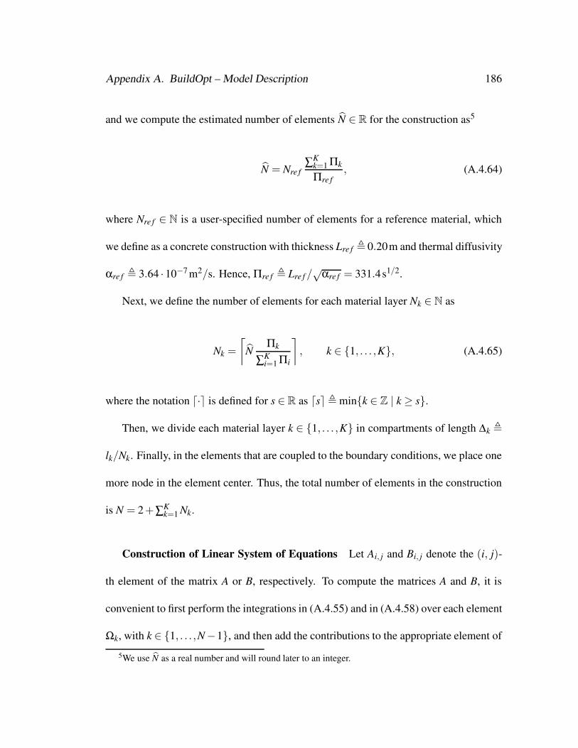
Appendix A. BuildOpt – Model Description 186
and we compute the estimated number of elements N ∈ R for the construction as5
N = Nre f∑K
k=1 Πk
Πre f, (A.4.64)
where Nre f ∈ N is a user-specified number of elements for a reference material, which
we define as a concrete construction with thickness Lre f , 0.20m and thermal diffusivity
αre f , 3.64 ·10−7 m2/s. Hence, Πre f , Lre f /√αre f = 331.4s1/2.
Next, we define the number of elements for each material layer Nk ∈ N as
Nk =
⌈N
Πk
∑Ki=1 Πi
⌉, k ∈ 1, . . . ,K, (A.4.65)
where the notation d·e is defined for s ∈ R as dse, mink ∈ Z | k ≥ s.
Then, we divide each material layer k ∈ 1, . . . ,K in compartments of length ∆k ,
lk/Nk. Finally, in the elements that are coupled to the boundary conditions, we place one
more node in the element center. Thus, the total number of elements in the construction
is N = 2+∑Kk=1 Nk.
Construction of Linear System of Equations Let Ai, j and Bi, j denote the (i, j)-
th element of the matrix A or B, respectively. To compute the matrices A and B, it is
convenient to first perform the integrations in (A.4.55) and in (A.4.58) over each element
Ωk, with k ∈ 1, . . . ,N−1, and then add the contributions to the appropriate element of
5We use N as a real number and will round later to an integer.

Appendix A. BuildOpt – Model Description 187
A or B.
To do so, we start by setting all elements of A and B equal to zero. For an element
Ωk, with k ∈ 1, . . . ,N−1, all basis functions are zero, except φk(·) and φk+1(·). Thus,
for the k-th element, we have the possible combinations (i, j) ∈ (k,k), (k,k + 1), (k +
1,k), (k+1,k+1). We evaluate the integrals in (A.4.55) for those combinations (setting
the boundary terms equal to zero for every index k), and then add the contributions of
each combination (i, j) to the element Ai, j or Bi, j.
After doing this for k ∈ 1, . . . ,N, we add the contributions of the boundary term of
(A.4.58) to the matrix B and the vector c. (Note that the matrix A is independent of the
boundary equations.)
Solution of the Equations The system of ordinary differential equations defined
in (A.4.60) is coupled to the ordinary differential equations that describe the time rate
of change of the room air temperatures and to the algebraic equations that describe the
window surface temperatures, which are assumed to have negligible thermal mass. The
coupling is due to the boundary conditions, which are functions of the room air temper-
ature and the surface temperatures of other constructions. All equations of this system
of differential algebraic equations are solved simultaneously using the commercial DAE
solver DASPK (Brenan et al., 1989; Brown et al., 1994, 1998). In Brown et al. (1994), it
is described how the DASPK solver computes consistent initial conditions η(x;z j)Nj=1.
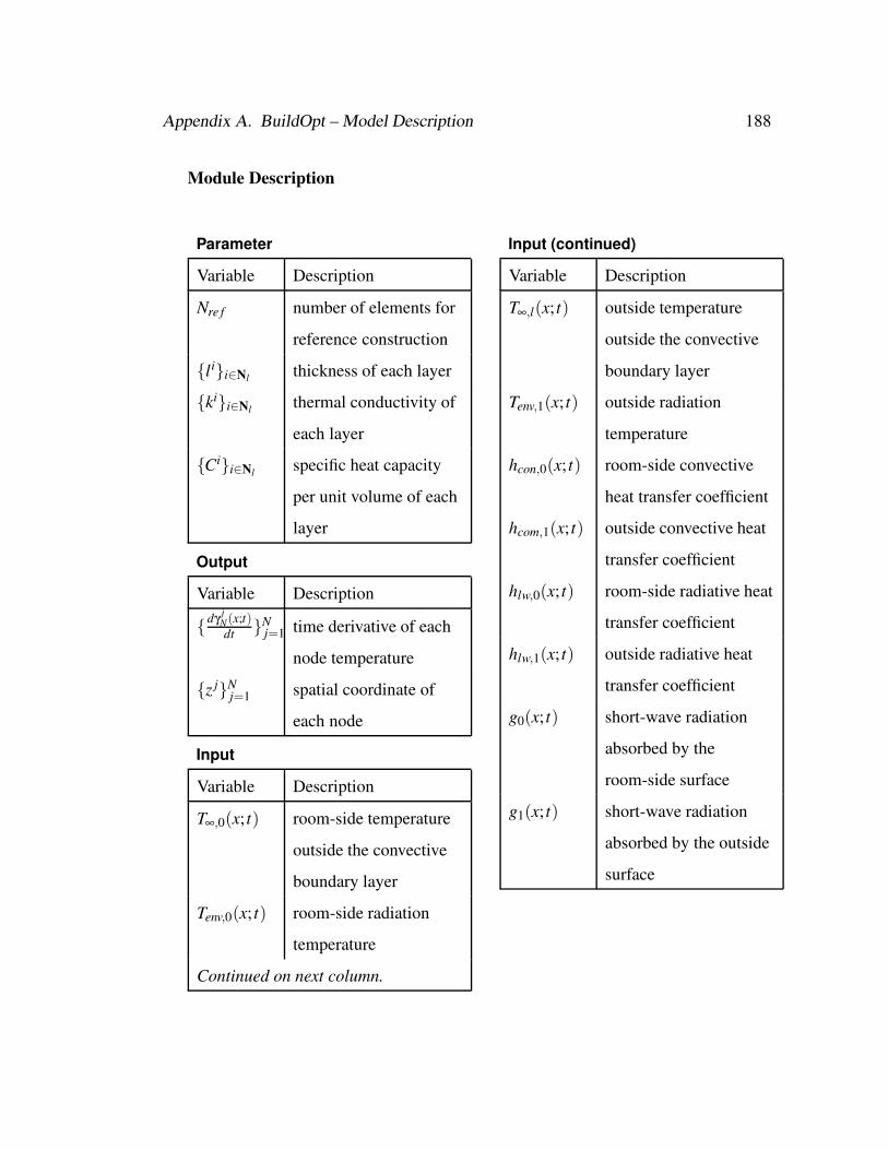
Appendix A. BuildOpt – Model Description 188
Module Description
Parameter
Variable Description
Nre f number of elements for
reference construction
lii∈Nl thickness of each layer
kii∈Nl thermal conductivity of
each layer
Cii∈Nl specific heat capacity
per unit volume of each
layer
Output
Variable Description
dγ jN(x;t)dt N
j=1 time derivative of each
node temperature
z jNj=1 spatial coordinate of
each node
Input
Variable Description
T∞,0(x; t) room-side temperature
outside the convective
boundary layer
Tenv,0(x; t) room-side radiation
temperature
Continued on next column.
Input (continued)
Variable Description
T∞,l(x; t) outside temperature
outside the convective
boundary layer
Tenv,1(x; t) outside radiation
temperature
hcon,0(x; t) room-side convective
heat transfer coefficient
hcom,1(x; t) outside convective heat
transfer coefficient
hlw,0(x; t) room-side radiative heat
transfer coefficient
hlw,1(x; t) outside radiative heat
transfer coefficient
g0(x; t) short-wave radiation
absorbed by the
room-side surface
g1(x; t) short-wave radiation
absorbed by the outside
surface

Appendix A. BuildOpt – Model Description 189
panesurface
outside room-side
A1
T 1,1
1 21
R1,1f R1,1
b
A2
T 2,2
3 42
R2,2f
AN
T N,N
2N−1 2NN
RN,Nb
T 1,N
R1,Nf
RN,1b
Figure A.8: Transmittance and absorbtance of a window with N panes (N > 1) andradiation source at the outside.
A.4.3.3 Window Simulation for Short-Wave Radiation
Introduction We will now present how the short-wave absorbtance and the transmit-
tance of each pane, and the short-wave transmittance of the window are computed for
a given angle of incidence, or, alternatively, for hemispherical irradiation. We will also
present how the front and the back reflectance of the window are computed. After de-
scribing how these properties are computed, we describe how they are modified to take
into account either an exterior or an interior shading device. The absorbtance of each
pane, the transmittance of the window, and the short-wave absorbtance of the interior
shading device are then used in the models that compute the temperature of the panes
and the daylight illuminance.

Appendix A. BuildOpt – Model Description 190
Our short-wave radiation model is similar to the WINDOW 4 model (Arasteh et al.,
1989; Finlayson et al., 1993). For the panes and surfaces, we will use the same number-
ing scheme as WINDOW 4 which is shown in Fig. A.8 and in Fig. A.10. First, we need
to introduce some definitions and nomenclatures.
Definitions and Nomenclatures Our computation is based on spectral properties that
are for energy calculations averaged over the whole solar spectrum and for daylighting
calculations averaged over the visible spectrum.6 Since the models are equal for the
radiation data averaged over the solar and for the radiation data averaged over the visible
spectrum, we will call these averaged properties for both spectra total properties.
The computation of the window properties are done for specular irradiation (i.e., for
a particular angle of incidence φi) and for hemispherical irradiation. Our model requires
as parameters the spectrally averaged glass properties for each pane at normal incidence
angle. In our model, we first convert these properties to specular and hemispherical prop-
erties for each pane, and then compute the properties for the window. We will denote
properties for normal incidence by P⊥, directional properties by P ± and hemispherical
properties by P∩.
We will compute a directional and a hemispherical total absorbtance of each pane,
6A database with these properties can be obtained from http://windows.lbl.gov/.

Appendix A. BuildOpt – Model Description 191
denoted by A ± , jNj=1 and by A∩, jN
j=1. They are defined for the j-th pane as the ra-
tio between the absorbed radiation q jabs and the total directional irradiation or the total
hemispherical irradiation, respectively, H ± ,1 and H∩,1. Hence,
A ± , j ,q ± , j
absH ± ,1 , (A.4.66a)
A∩, j ,q∩, j
absH∩,1 . (A.4.66b)
Similarly, the directional and hemispherical total transmittance of the window, T ± and
T∩, are defined as the ratio between the radiation transmitted through the window, H ±Tor H∩T , and the total directional or hemispherical irradiation at the window outside, H ± ,1
or H∩,1, i.e.,
T ± ,H ±T
H ± ,1 , (A.4.66c)
T∩ ,H∩T
H∩,1 . (A.4.66d)
Most of the equations apply for directional as well as for hemispherical irradiation. If no
ambiguity arises, we will omit the superscript.
To facilitate the notation, we introduce an index set that contains the index of all

Appendix A. BuildOpt – Model Description 192
panes. For a window with N panes, we define this index set as
N , 1, . . . , N. (A.4.67a)
We also introduce an index set that contains certain directional modes of irradiations: it
contains for directional irradiation the incidence angles φi ∈ 0, 10, . . . , 90 and an
index for hemispherical irradiation. We define this index set as
I , 0, 10, . . . , 90, hemispherical. (A.4.67b)
We also introduce a front absorbtance A jf and a back absorbtance A j
b for the j-th
pane. These terms are defined as the absorbtance that the pane would have if the pane
was standing isolated with no other panes present, and if the irradiation was only from
the front side or only from the back side, respectively. Front and back absorbtance are
equal for uncoated glass, but in general different for coated glass.
In Fig. A.8, T i, j denotes the total transmittance through the panes i and j, and through
all panes in between, Ri, j denotes the total reflectance from pane i to j as if they were
standing alone. Reflection is denoted by a subscript “ f ” if the irradiation is from the
front side (i.e., the outside) and by a subscript “b” if the irradiation is from the back side
(i.e., the room-side).

Appendix A. BuildOpt – Model Description 193
Short wave radiation can strike the window from the outside (e.g., solar radiation)
and from the inside (e.g., solar radiation reflected in the room and lighting). Thus, equa-
tion (A.4.66) depends on whether the irradiation comes from outside or from inside.
Properties that correspond to irradiation from outside and from inside will be denoted
by P→ and P←, respectively. If no ambiguity arises, we will omit the subscript. Note
that we do not flip the counter for the pane and the subscript for the front and back if we
change the radiation source from the outside to the inside, since our notation is based
on the geometry defined in Fig. A.8. For example, RN,2b is the reflectance of a window
where the outside pane is removed and the radiation source is placed in the room.
Model Parameter The model uses the following glass properties:
T⊥, j, jNj=1 spectrally averaged transmittance of each pane at normal incidence,
R⊥, j, jf N
j=1 spectrally averaged front reflectance of each pane at normal
incidence, and
R⊥, j, jb N
j=1 spectrally averaged back reflectance of each pane at normal incidence.
If an exterior, or alternatively, an interior shading device is present, then its trans-
mittance and reflectance must be specified by the user. For an exterior shading device,
τ1 denotes the total transmittance and ρ1 denotes the total reflectance. For an interior
shading device, the corresponding symbols are τN and ρN .
Angular Properties of Glass Transmittance and reflectance of glass do not vary much
for incidence angles smaller than 50 to 60, but approach 0 or 1, respectively, as the in-

Appendix A. BuildOpt – Model Description 194
cidence angle tends to 90. During most of the time, the incidence angle of the sun is
larger than 45. Therefore, the directional dependency of the glass properties at shallow
incidence angles need to be taken into account properly.
To compute the angular dependency of the solar transmittance and the solar front and
back reflectance, we use a similar model as the WINDOW 4 program (Finlayson et al.,
1993). The model uses the solar transmittance T⊥ and the solar front and back re-
flectance R⊥f and R⊥b , all at normal incidence angle, of a single pane and computes their
directional values using a regression fit. The regression fits were developed for uncoated
clear glass and for uncoated bronze glass. However, the regressions are in WINDOW 4
and in our model as well used for coated glass and for uncoated glass. If T⊥ > 0.645,
the fit for clear glass is used, otherwise the fit for bronze glass is used.
The angular variation of the transmittance and the reflectance are
T ± (φ) =4
∑k=0
Tk cosk(φ), (A.4.68a)
R ± (φ) =4
∑k=0
Rk cosk(φ)− T ± (φ), (A.4.68b)
where φ , 0 for normal incidence and the coefficients Tk4k=0 and Rk4
k=0 are listed in
Tab. A.2.
After computing (A.4.68), the angular transmittance, the angular front and the angu-

Appendix A. BuildOpt – Model Description 195
index k0 1 2 3 4
If T⊥ > 0.645: Tk −0.0015 3.355 −3.840 1.460 0.0288If T⊥ > 0.645: Rk 0.999 −0.563 2.043 −2.532 1.054If T⊥ ≤ 0.645: Tk −0.002 2.813 −2.341 −0.05725 0.599If T⊥ ≤ 0.645: Rk 0.997 −1.868 6.513 −7.862 3.225
Table A.2: Coefficients used in the regression formula (A.4.68), reproduced fromFinlayson et al. (1993).
lar back reflectance are computed as
T ± (φ) =
T⊥ T ±clr(φ), if T⊥ > 0.645,
T⊥ T ±bnz(φ), otherwise,
(A.4.69a)
R ± (φ) =
R⊥(1− R ±clr(φ)
)+ R ±clr(φ), if T⊥ > 0.645,
R⊥(1− R ±bnz(φ)
)+ R ±bnz(φ), otherwise.
(A.4.69b)
The hemispherical values are computed as
T∩ = ² π/20 T ± (φ) cos(φ) sin(φ)dφ
² π/20 cos(φ) sin(φ)dφ
= 2 π/2
0T ± (φ) cos(φ) sin(φ)dφ, (A.4.70a)
R∩ = ² π/20 R ± (φ) cos(φ) sin(φ)dφ
² π/20 cos(φ) sin(φ)dφ
= 2 π/2
0R ± (φ) cos(φ) sin(φ)dφ. (A.4.70b)
The equations (A.4.70) are integrated numerically using the trapezoidal rule. For the

Appendix A. BuildOpt – Model Description 196
numerical integration, we use the support points T ± (φi), R ± f (φi) and R ±b (φi), with φi ∈
0, 10, . . . , 90, which we compute using equation (A.4.69).
Specular and Hemispherical Transmittance and Reflectance We will now describe
how we obtain the following properties for directional irradiation at incidence angles
φi ∈ [0, 90] and for hemispherical irradiation:
1. the total transmittances from outside to inside and from inside to outside for direc-
tional and for hemispherical irradiation, i.e., T ± ,1,N , T ± ,N,1, T∩,1,N , T∩,N,1, and
2. the window’s front and back reflectances for directional and for hemispherical
irradiation, i.e., R ± ,1,Nf , R ± ,N,1
b , R∩,1,Nf , R∩,N,1
b .
We will first develop a model that computes the above properties for radiation strik-
ing the window from the outside. To simplify the notation, we will omit the subscript
“→” and the superscript “^” or “∩” in the equations (A.4.71) to (A.4.78c) below. The
model will be developed for a single pane window, for a double pane window, and for
a window with more than two panes. Based on this development, we present equations
that are valid for any window with more than one pane. The model takes into account
multiple reflections between panes. We will assume that the window consists of infinite
large parallel panes, and hence, we will neglect frame effects. How to take into account
an exterior or an interior shading device will be presented later.

Appendix A. BuildOpt – Model Description 197
Single Pane Window For single pane windows, we have N = 1 and hence
T 1,N = T 1,1, R1,Nf = R1,1
f , RN,1b = R1,1
b . (A.4.71)
Double Pane Window We will first show how to obtain the transmittance and then
the reflectance. Let H1 denote the irradiation on the front of pane number 1, and let H2
denote the irradiation on the front of pane number 2. Then, we have
H1 T 1,N = HN T N,N, (A.4.72)
where T 1,N and HN are unknown. HN is the sum of the radiation transmitted through
pane 1, which is equal to H1 T 1,1, and the fraction of it which underwent multiple reflec-
tions between pane 1 and pane N. By using the geometric series
∞
∑k=0
axk =a
1− x, for |x|< 1, a ∈ R, (A.4.73)
we can write
HN = H1 T 1,1 +H1 T 1,1 (RN,Nf R1,1
b )+ . . .
= H1 T 1,1∞
∑k=0
(RN,Nf R1,1
b )k =H1 T 1,1
1−RN,Nf R1,1
b
. (A.4.74a)

Appendix A. BuildOpt – Model Description 198
Substituting (A.4.74a) in (A.4.72) and solving for T 1,N yields
T 1,N =T 1,1 T N,N
1−RN,Nf R1,1
b
. (A.4.74b)
The reflectance R1,Nf is defined as the ratio between the radiation that is reflected
and leaves the window to the outside (at the front surface) and the irradiation H1. It is
composed of the front reflectance at pane number 1 and the part of the radiation that has
been transmitted through pane number 1, underwent multiple reflections between pane
number N and pane number 1 and then has been transmitted again through pane number
1. Thus,
H1R1,Nf = H1 R1,1
f +H1 T 1,1 RN,Nf T 1,1 +H1 T 1,1 RN,N
f
(R1,1
b RN,Nf
)T 1,1
+H1 T 1,1 RN,Nf
(R1,1
b RN,Nf
)2T 1,1 + . . .
= H1
(R1,1
f +(T 1,1)2
RN,Nf
∞
∑k=0
(R1,1
b RN,Nf
)k)
= H1
R1,1
f +
(T 1,1)2 RN,N
f
1−R1,1b RN,N
f
, (A.4.75a)
or after dividing by H1,
R1,Nf = R1,1
f +
(T 1,1)2 RN,N
f
1−RN,Nf R1,1
b
. (A.4.75b)
The back reflectance, i.e., the reflectance if the irradiation source is inside the building,
is obtained from geometric considerations by changing in (A.4.75b) the subscript “b”

Appendix A. BuildOpt – Model Description 199
with “ f ” (and vice versa) and the index “1” with “N” (and vice versa). Thus,
RN,1b = RN,N
b +
(T N,N)2 R1,1
b
1−RN,Nf R1,1
b
. (A.4.75c)
Window with Three or More Panes For a window with more than two panes, we
treat the first (N−1) panes as if they were one pane with properties T 1,N−1, R1,N−1f and
RN−1,1b . Thus, we obtain
T 1,N =T 1,N−1 T N,N
1−RN,Nf RN−1,1
b
, (A.4.76a)
R1,Nf = R1,N−1
f +
(T 1,N−1)2 RN,N
f
1−RN,Nf RN−1,1
b
, (A.4.76b)
RN,1b = RN,N
b +
(T N,N)2 RN−1,1
b
1−RN,Nf RN−1,1
b
. (A.4.76c)
Note that the equations (A.4.76) are similar to the equations for double pane windows.
Furthermore, we can replace in (A.4.76) the superscript “1” with any i ∈ 1, . . . , (N−
1). Therefore we can state the following recursive computation procedure for windows
with N > 1.
General Computation Procedure for Windows with more than one Pane We
will describe the computation procedure by two indexed loops. The properties T i, j, Ri, jf
and Ri, jb are obtained using an outer loop with loop counter i = 1, . . . , (N− 1) and an
inner loop with loop counter j = (i + 1), . . . , N. Inside the loops, we do the following

Appendix A. BuildOpt – Model Description 200
computations:
First, we compute the denominator of (A.4.76), which is
ai, j = 1−R j, jf R j−1,i
b , (A.4.77)
and then we compute
T i, j =T i, j−1 T j, j
ai, j , (A.4.78a)
Ri, jf = Ri, j−1
f +(T i, j−1)2 R j, j
f
ai, j , (A.4.78b)
R j,ib = R j, j
b +(T j, j)2 R j−1,i
bai, j . (A.4.78c)
This ends the computations inside the loops.
Specular and Hemispherical Absorbtance We will now show how to compute the
short-wave absorbtance of each pane for directional irradiation, which we denote by
A ± , j→ N
j=1 and A ± , j← N
j=1, and for hemispherical irradiation, which we denote by A∩, j→ N
j=1
and A∩, j← N
j=1. The model is based on the results described in (A.4.78).
We will develop the model for the situation where the radiation source is outside
the building. We will again omit the superscripts “^” and “∩”, because the models are
identical for both situations.

Appendix A. BuildOpt – Model Description 201
We first compute the front absorbtance. For single pane windows, they are
A1→ = 1−T 1,1−R1,1
f , (A.4.79)
A1← = 1−T 1,1−R1,1
b , (A.4.80)
and for multi pane windows, they are, for j ∈ N,
A jf = 1−T j, j−R j, j
f , (A.4.81a)
A jb = 1−T j, j−R j, j
b . (A.4.81b)
Next, to facilitate the formulation, we introduce the auxiliary variables
T 1,0 = 1, R0,1b = 0, RN+1,N
f = 0. (A.4.82)
Let H1 denote the irradiation source, placed outside the building. Because the ab-
sorbtance A j→ is composed of the back and the front absorbtance of the j-th pane, we

Appendix A. BuildOpt – Model Description 202
can write for any pane, with j ∈ N,
H1 A j→ = H1
(T 1, j−1 +T 1, j−1
(R j,N
f R j−1,1b
)+T 1, j−1
(R j,N
f R j−1,1b
)2+ . . .
)A j
f
+H1(
T 1, j R j+1,Nf +T 1, j R j+1,N
f
(R j,1
b R j+1,Nf
)+ . . .
)A j
b
= H1
(T 1, j−1
∞
∑k=0
(R j,N
f R j−1,1b
)k)
A jf
+H1
(T 1, j R j+1,N
f
∞
∑k=0
(R j,1
b R j+1,Nf
)k)
A jb. (A.4.83a)
Using the geometric series introduced in (A.4.73) and dividing by H1 yields
A j→ =
T 1, j−1
1−R j,Nf R j−1,1
b
A jf +
T 1, j R j+1,Nf
1−R j,1b R j+1,N
f
A jb. (A.4.83b)
If either of the denominator in (A.4.83b) is zero, then no radiation reaches the pane j
and hence we set A j→ = 0.
Next, we compute (A.4.77) to (A.4.78c) and (A.4.83b) for the situation where the
radiation source is inside the building. This yields the remaining terms of (A.4.78), with
j < i, and the absorbtances A∩, j← N
j=1. Since we assume the short-wave radiation from
the room to be diffuse, we compute directional and hemispherical values for (A.4.78),
but only hemispherical values for (A.4.83b).
To facilitate the calculation, we will introduce dummy variables, indicated by a tilde,
i.e., we will write “P” instead of “P”, that can be used in equations (A.4.77), (A.4.78),
Appendix A. BuildOpt – Model Description 203
(A.4.81), (A.4.82) and (A.4.83b). In particular, we will define the dummy variables, for
all i ∈ I,
T i, j, jNj=1 = T i, j, j1
j=N ,
Ri, j, jf N
j=1 = Ri, j, jb 1
j=N , Ri, j, jb N
j=1 = Ri, j, jf 1
j=N. (A.4.84)
Then, we compute (A.4.77), (A.4.78), (A.4.81), (A.4.82) and (A.4.83b), again with
the loop counter counting upward (as indicated) whereas in all equations every property
is replaced with its dummy variable as defined in (A.4.84). This yields, for all i ∈ I, with
outer loop i = 1, . . . , (N−1) and with inner loop j = (i+1), . . . , N, the transmittances
T i,N+1−i,N+1− j = T i,i, j, (A.4.85a)
and the absorbtances
Ai, j←1
j=N = Ai, j→N
j=1. (A.4.86a)
Exterior and Interior Shading Device The models presented above are all for win-
dows with no interior or exterior shading device.
We will now develop expressions that correct the values obtained by the above mod-
els so that either an interior or an exterior shading device is taken into account. We will
assume that the shading devices are diffuse reflectors, that only one shading device is

Appendix A. BuildOpt – Model Description 204
active at any time and that the irradiation from the room side is diffuse. We will de-
velop corrections for the absorbtances A∩, j← and Ai, j
→, and for the transmittances T i,1,N
and T∩,N,1, with i ∈ I and j ∈ N. We will also develop an equation to compute what ra-
diation is absorbed by the room-side shading device, because this absorbed energy will
be released by convection and by infrared radiation to the room.
Since all equations for directional irradiation are also valid for hemispherical irra-
diation, we will develop the model for directional irradiation only. The expressions for
hemispherical irradiation can be obtained by replacing the superscript “^” with the su-
perscript “∩”.
First, we will assume that the radiation source is on the outside.
Exterior Shading Device, Irradiation from Outside Exterior shading devices
reduce the irradiation that strikes the surface number 1. Since the energy transmitted
through the panes and the energy absorbed by each pane is proportional to the transmit-
tance or the absorbtance, respectively, and proportional to the irradiation, we will reduce
T 1,N and A j→N
j=1 instead of reducing the incoming radiation.
Let ρ1 denote the reflectance and let τ1 denote the transmittance of the exterior shad-
ing device. Let H ±0 denote the irradiation outside the exterior shading device, and let
H ± ,1 denote the irradiation on the pane number 1 (see Fig. A.8). The irradiation H ± ,1
is composed of the fraction of H ±0 that has been transmitted through the shading device

Appendix A. BuildOpt – Model Description 205
(and has not yet been reflected), and the radiation that underwent multiple reflections
between the window and the shading device. We will assume that the reflection from the
shading device is diffuse. However, the irradiation (H ±0 τ1) is directional. Thus, we have
H ± ,1 = H ±0 τ1 +H ±0 τ1(
R ± ,1,Nf ρ1
)+H ±0 τ1
(R ± ,1,N
f ρ1) (
R∩,1,Nf ρ1
)
+H ±0 τ1(
R ± ,1,Nf ρ1
) (R∩,1,N
f ρ1)2
+ . . .
= H ±0 τ1 +H ±0 τ1(
R ± ,1,Nf ρ1
) ∞
∑k=0
(R∩,1,N
f ρ1)k
= H ±0 τ1 +H ±0 τ1 R ± ,1,Nf ρ1
1−R∩,1,Nf ρ1
. (A.4.87)
Equation (A.4.87) shows that the irradiation that strikes the pane number 1 is attenuated
by a factor
c ± ,1 , τ1
(1+
R ± ,1,Nf ρ1
1−R∩,1,Nf ρ1
). (A.4.88a)
Therefore, the absorbtance of each pane j ∈ N is, if the window has an exterior shading
device,
A ± , jτ1,→ = c ± ,1 A ± , j
→ . (A.4.88b)
Since the energy transmitted through the overall construction is also proportional to the
irradiation, we have for the window transmittance with exterior shading device
T ± ,1−τ,N = c ± ,1 T ± ,1,N . (A.4.88c)
Appendix A. BuildOpt – Model Description 206
The equations (A.4.88) are also valid for hemispherical irradiation.
Interior Shading Device, Irradiation from Outside We will now develop an
equation that accounts for the increase in absorbed radiation of each pane due to the
radiation that is reflected at an interior shading device. We will also develop an equation
for the radiation that is absorbed by the shading device, and corrections for the transmit-
tance of the window including shading device. We will assume that the shading device
is a diffuse reflector with reflectance ρN and transmittance τN .
Let ∆H j→, f denote the increase in irradiation at the front side of the j-th pane due
to the radiation that is reflected at the interior shading device. We will introduce the
dummy variables R∩,0,1b = 0. Then, for j ∈ N,
∆H j→, f = H1 T ± ,1,N ρN
∞
∑k=0
(R∩,N,1
b ρN)k
T∩,N, j R∩, j−1,1b
= H1 T ± ,1,N ρN T∩,N, j R∩, j−1,1b
1−R∩,N,1b ρN
. (A.4.89a)
Similarly, by introducing the dummy variable T ∩,N,N+1 = 1, the increase in irradiation
at the back surface can be described as, with j ∈ N,
∆H j→,b = H1 T ± ,1,N ρN
∞
∑k=0
(R∩,N,1
b ρN)k
T∩,N, j+1
= H1 T ± ,1,N ρN T∩,N, j+1
1−R∩,N,1b ρN
. (A.4.89b)

Appendix A. BuildOpt – Model Description 207
By assumption, the shading device reflects diffusely, and hence ∆H j→, f and ∆H j
→,b
are diffuse irradiations. Therefore, for j ∈ N, with R∩,0,1b = 0 and T∩,N,N+1 = 1, the
directional absorbtances for the panes are, if the window has an interior shading device,
A ± , jτN ,→ = A ± , j
→ +T ± ,1,N ρN T∩,N, j R∩, j−1,1
b
1−R∩,N,1b ρN
A∩, jf +
T ± ,1,N ρN T∩,N, j+1
1−R∩,N,1b ρN
A∩, jb , (A.4.90)
where A∩, jf and A∩, j
b are defined in (A.4.81).
Let A ± ,τN
→ denote the fraction of the outside irradiation H1 that is absorbed by the
interior shading device. It can be obtained from
H1 A ± ,τN
→ = H1 T ± ,1,N∞
∑k=0
(ρN R∩,N,1
b
)k (1−ρN− τN)
= H1 T ± ,1,N
1−ρN R∩,N,1b
(1−ρN− τN) . (A.4.91a)
Thus, after dividing by H1, we have
A ± ,τN
→ =T ± ,1,N
1−ρN R∩,N,1b
(1−ρN− τN) . (A.4.91b)
Let H ± ,1,N+τ denote the directional transmittance through all panes and through the
Appendix A. BuildOpt – Model Description 208
shading device. We have
H1 H ± ,1,N+τ = H1 T ± ,1,N
1−ρN R∩,N,1b
τN. (A.4.92a)
After dividing by H1, we obtain the overall transmittance of the window and the shading
device as
T ± ,1,N+τ =T ± ,1,N
1−ρN R∩,N,1b
τN. (A.4.92b)
Exterior Shading Device, Irradiation from Inside We will now assume that a
diffuse radiation source is inside the room. Let HN denote the irradiation at the pane N
from the room side. We define the dummy variables T ∩,1,0 = 1 and R∩,N+1,Nf = 0. Then,
similarly as in (A.4.89), for j ∈ N, the increase in irradiation at the pane front and back
surface is
∆H∩, j←, f = HN T∩,N,1 ρ1
∞
∑k=0
(R∩,1,N
f ρ1)k
T∩,1, j−1
= HN T∩,N,1 ρ1 T∩,1, j−1
1−R∩,1,Nf ρ1
, (A.4.93a)
∆H∩, j←,b = HN T∩,N,1 ρ1
∞
∑k=0
(R∩,1,N
f ρ1)k
T∩,1, j R∩, j+1,Nf
= HN T∩,N,1 ρ1 T∩,1, j R∩, j+1,Nf
1−R∩,1,Nf ρ1
. (A.4.93b)

Appendix A. BuildOpt – Model Description 209
Therefore, for j ∈ N, we can obtain for windows with exterior shading device the ab-
sorbtances as
A∩, jτ1,← = A∩, j
← +T∩,N,1 ρ1 T∩,1, j−1
1−R∩,1,Nf ρ1
A∩, jf +
T∩,N,1 ρ1 T∩,1, j R∩, j+1,Nf
1−R∩,1,Nf ρ1
A∩, jb , (A.4.94)
where A∩, jf and A∩, j
b are as in (A.4.81).
The transmittance through the window and shading device is
T∩,N,1−τ = T∩,N,1∞
∑k=0
(ρ1 R∩,1,N
f
)kτ1 =
T∩,N,1 τ1
1−ρ1 R∩,1,Nf
. (A.4.95)
To obtain the distribution of the short-wave radiation in the room enclosure, we need to
know the reflectance of the window with shading device. It is obtained from the radiation
balance
HN R∩,N,1−τb = HN R∩,N,1
b +HN T∩,N,1 ρ1∞
∑k=0
(R∩,1,N
f ρ1)k
T∩,1,N. (A.4.96)
Thus,
R∩,N,1−τb = R∩,N,1
b +T∩,N,1 ρ1 T∩,1,N
1−R∩,1,Nf ρ1
. (A.4.97)
Interior Shading Device, Irradiation from Inside To obtain the absorbtance of
each pane and the overall transmittance, we will compute how much the irradiation on

Appendix A. BuildOpt – Model Description 210
pane N is attenuated due to the interior shading device. Let H∩,r denote the irradiation
on the room side facing surface of the shading device, and let H∩,N denote the room-side
irradiation on the pane N. Then, we have
H∩,N = H∩,r τN
(1+R∩,N,1
b ρN∞
∑k=0
(R∩,N,1
b ρN)k)
. (A.4.98)
Thus, the irradiation is attenuated by a factor
c∩,N = τN
(1+
R∩,N,1b ρN
1−R∩,N,1b ρN
). (A.4.99)
Hence, the absorbtance of each pane and the overall transmittance of the window and
the shading device is, for j ∈ N,
A∩, jτN ,← = c∩,N A∩, j
← , (A.4.100a)
T∩,N+τ,1 = c∩,N T∩,N,1. (A.4.100b)
For the thermal heat balance of the zone, we also need to know what part of H∩,r is
absorbed by the shading device. Let qabs denote the radiation that is absorbed by the
shading device for a given room-side irradiation H∩,r. We define the absorbtance of the
shading device for room-side irradiation by
AτN
← ,qabs
H∩,r . (A.4.101)
Appendix A. BuildOpt – Model Description 211
We can obtain AτN
← from
H∩,r AτN
← = H∩,r (1− τN−ρN)
+H∩,r τN R∩,N,1b
∞
∑k=0
(R∩,N,1
b ρN)k (
1− τN−ρN) . (A.4.102)
Thus,
AτN
← =(1− τN−ρN)
(1+
τN R∩,N,1b
1−R∩,N,1b ρN
). (A.4.103)
We also need to know the back reflectance of the window with interior shading device,
which we denote by R∩,N+τ,1b . Recalling that c∩,N , defined in (A.4.99), already takes
multiple reflections between the shading device and the panes into account, we can write
H∩,r R∩,N+τ,1b = H∩,r ρN + c∩,N H∩,r R∩,N,1
b τN. (A.4.104)
Hence,
R∩,N+τ,1b = ρN + c∩,N R∩,N,1
b τN. (A.4.105)

Appendix A. BuildOpt – Model Description 212
Module DescriptionParameter
Variable Description
N number of panes
T⊥, j, j j∈N solar transmittance of
panes at normal
incidence
R⊥, jf j∈N front solar reflectance
of panes at normal
incidence
R⊥, jb j∈N back solar reflectance of
panes at normal
incidence
τ1 solar transmittance of
exterior shading device
(or 0 if no shading
device is installed)
ρ1 solar reflectance of
exterior shading device
(or 0 if no shading
device is installed)
Continued on next column.
Parameter (continued)
Variable Description
τN solar transmittance of
interior shading device
(or 0 if no shading
device is installed)
ρN solar reflectance of
interior shading device
(or 0 if no shading
device is installed)

Appendix A. BuildOpt – Model Description 213
Output
Variable Description
Ai, j→i∈I, j∈N absorbtance for
irradiation from
outside
Ai, j←i∈I, j∈N absorbtance for
irradiation from
inside
Ai, jτ1,→i∈I, j∈N absorbtance for
irradiation from
outside, exterior
shading device
Ai, jτN ,→i∈I, j∈N absorbtance for
irradiation from
outside, interior
shading device
T i,1,Ni∈I transmittance from
outside to inside,
no shading device
Continued on next column.
Output (continued)
Variable Description
T i,1−τ,Ni∈I transmittance from
outside to inside
with exterior
shading device
T i,1,N+τi∈I transmittance from
outside to inside
with interior
shading device
A∩, jτ1,← j∈N hemispherical
absorbtance for
irradiation from
inside, exterior
shading device
A∩, jτN ,← j∈N hemispherical
absorbtance for
irradiation from
inside, interior
shading device
Continued on next page.

Appendix A. BuildOpt – Model Description 214
Output (continued)
Variable Description
R∩,N,1−τb back reflectance
with exterior
shading device
R∩,N+τ,1b back reflectance
with interior
shading device
A ± ,τN
→ absorbtance of
interior shading
device for
irradiation from
outside
AτN
← absorbtance of
interior shading
device for
irradiation from
inside

Appendix A. BuildOpt – Model Description 215
Algorithm – Angular properties of glass
1: data R⊥f , R⊥b , T⊥
2: if T⊥ > 0.645 then
3: select from Tab. A.2: Tk4k=0 = Tclr,k4
k=0; Rk4k=0 = Rclr,k4
k=0;
4: else
5: select from Tab. A.2: Tk4k=0 = Tbnz,k4
k=0; Rk4k=0 = Rbnz,k4
k=0;
6: end if
7: for all φi ∈ (i−1)π/189i=2 do
8: T ± (φi)(A.4.68a)←− Tk4
k=0, φi;
9: R ± (φi)(A.4.68b)←− Rk4
k=0, φi;
10: T ± (φi)(A.4.69a)←− T⊥, T ± (φi);
11: R ± f (φi)(A.4.69b)←− R⊥f , R ± (φi);
12: R ±b (φi)(A.4.69b)←− R⊥b , R ± (φi);
13: end for
14: assign R ± f (φi = 0) = R⊥f , R ±b (φi = 0) = R⊥b , T ± (φi = 0) = T⊥;
15: assign R ± f (φi = π/2) = R ±b (φi = π/2) = 1, T ± (φi = π/2) = 0;
16: T∩(A.4.70a)←− T ± (φi)10
i=1;
17: R∩f(A.4.70b)←− R ± f (φi)10
i=1;
18: R∩b(A.4.70b)←− R ±b (φi)10
i=1;
19: output T ii∈I, Rif i∈I, Ri
bi∈I;

Appendix A. BuildOpt – Model Description 216
Algorithm – Window properties, no shading device
1: data T i, j, j j∈Ni∈I, Ri, j, jf j∈Ni∈I, R j, j
b j∈N;
2: if N = 1 then
3: Single pane window4: for all φi ∈ I do
5: T 1,N , R1,Nf , RN,1
b , A1→, A1
←(A.4.71)←− T 1,1, R1,1
f , R1,1b ;
6: A1→, A1
←(A.4.80)←− T 1,1, R1,1
f , R1,1b ;
7: end for
8: end if
9: Continued on next page.

Appendix A. BuildOpt – Model Description 217
Algorithm – Window properties, no shading device (continued)
10: if N > 1 then
11: Multi-pane window12: for all φi ∈ I do
13: for i = 1, . . . , (N−1) do
14: for j = (i+1), . . . , N do
15: ai, j(A.4.77)←− R j, jf , R j−1,i
b ;
16: if ai, j = 0 then
17: set Ti, j = 0; Ri, jf = R j,i
b = 1;
18: else
19: T i, j(A.4.78a)←− T i, j−1, T j, j, ai, j;
20: Ri, jf
(A.4.78b)←− Ri, j−1f , R j, j
f , T i, j−1, ai, j;
21: R j,ib
(A.4.78c)←− R j, jb , R j−1,i
b , T j, j, ai, j;
22: end if
23: end for
24: end for
25: introduce (A.4.82) T 1,0 = 1, R0,1b = 0, RN+1,N
f = 0;
26: for all j ∈ N do
27: A jf(A.4.81a)←− T j, j, R j, j
f ;
28: A jb(A.4.81b)←− T j, j, R j, j
b ;
29: A j→
(A.4.83b)←− T 1, j−1, R j,Nf , R j−1,1
b , R j+1,Nf , R j,1
b , T 1, j, A jf , A j
b;
30: save A jf ,A
jb,A
j→;
31: end for
32: end for
33: end if
34: Continued on next page.
Appendix A. BuildOpt – Model Description 218
Algorithm – Window properties, no shading device (continued)
35: for hemispherical irradiation only do
36: assign (A.4.84);
37: execute Step 2 to Step 33, but in Step 30, do not save A jf ,A
jb: ;
38: assign (A.4.85) and (A.4.86);
39: end for
40: return T i,1,Ni∈I, Ri, jf j∈Ni∈I, R∩, j
b j∈N, Ai, j→ j∈Ni∈I, A∩, j
← j∈N;
Algorithm – Irradiation from Outside, Exterior Shading Device
1: data ρ1, τ1, Ri,1,Nf i∈I, Ai, j
→ j∈Ni∈I, T i,1,Ni∈I;
2: for all φi ∈ I do
3: ci,1(A.4.88a)←− τ1, ρ1, Ri,1,Nf , R∩,1,N
f ;
4: for all j ∈ N do
5: Ai, jτ1,→
(A.4.88b)←− ci,1, Ai, j→;
6: end for
7: T i,1−τ,N(A.4.88c)←− ci,1, T i,1,N;
8: end for

Appendix A. BuildOpt – Model Description 219
Algorithm – Irradiation from Outside, Interior Shading Device
1: data ρN, τN , T i,1,Ni∈I, T∩,N, j j∈N, R∩, j,1b j∈N,
Ai, j→ j∈Ni∈I, A∩, j
f j∈N, A∩, jb j∈N;
2: introduce R∩,0,1b = 0 and T∩,N,N+1 = 1;
3: for all φi ∈ I do
4: for all j ∈ N do
5: Ai, jτN ,→
(A.4.90)←− ρN, T i,1,N, T∩,N, j+1, T∩,N, j, R∩, j−1,1b , R∩,N,1
b , R∩,N,1b , Ai, j
→,
6: A∩, jf , A∩, j
b ;
7: end for
8: Ai,τN
→(A.4.91b)←− τN, ρN, T i,1,N, R∩,N,1
b ;
9: T i,1,N+τ(A.4.92b)←− τN, ρN, T i,1,N, R∩,N,1b ;
10: end for
Algorithm – Irradiation from Inside, Exterior Shading Device
1: data ρ1, T∩,N,1, T∩,1, j j∈N, R∩, j,Nf j∈N, R∩,N,1
b ,
A∩, jf j∈N, A∩, j
b j∈N, A∩, j← j∈N;
2: introduce T∩,1,0 = 1 and R∩,N+1,Nf = 0;
3: for all j ∈ N do
4: A∩, jτ1,←
(A.4.94)←− ρ1, A∩, j← , T∩,N,1, T∩,1, j−1, T∩,1, j, R∩,1,N
f , R∩, j+1,Nf ,
5: A∩, jf , A∩, j
b ;
6: end for
7: R∩,N,1−τb
(A.4.97)←− ρ1, R∩,1,Nf , R∩,N,1
b , T∩,N,1, T∩,1,N;

Appendix A. BuildOpt – Model Description 220
Algorithm – Irradiation from Inside, Interior Shading Device
1: data ρN, τN , R∩,N,1b , A∩, j
← j∈N;
2: c∩,N(A.4.99)←− ρN, τN, R∩,N,1b ;
3: for all j ∈ N do
4: A∩, jτN ,←
(A.4.100a)←− c∩,N, A∩, j← ;
5: end for
6: AτN
←(A.4.103)←− ρN, τN, R∩,N,1
b ;
7: R∩,N+τ,1b
(A.4.105)←− ρN , τN, c∩,N, R∩,N,1b ;

Appendix A. BuildOpt – Model Description 221
Sun beams
ss y
win
hh ove
wwove
(a) Side view.
Sun beamsww ove
∆φ
wwove
~~
(b) Top view.
Figure A.9: Infinite long window overhang.
A.4.3.4 Window Overhang
Introduction We will now present a simple model for window overhangs. The win-
dow overhang is assumed to be of infinite length, which allows neglecting end effects.
The model is based on the geometric data ywin(x), hove and wove(x) which are shown
in Fig. A.9, and on the wall azimuth φp(x), the solar azimuth φs(t) and the solar zenith
angle θs(t), which are described in Section A.4.2.1 on page 141.
Mathematical Description Let φp(x) be the azimuth of a vertical wall, and let φs(t) be
the azimuth of the sun, with φp(x) , 0 and φs(t) , 0 due south. Then, the solar azimuth
is, relative to the wall azimuth,
∆φ(x, t) = φs(t)−φp(x). (A.4.106)

Appendix A. BuildOpt – Model Description 222
Let wove denote the width of the overhang as shown in Fig. A.9. The horizontal compo-
nent wove of the distance which the sun beam travels below the overhang before it hits
the wall is
wove(x, t) =1
cos∆φ(x, t)wove(x). (A.4.107a)
When the window is exposed to direct radiation, we have ∆φ(x, t)∈ [−90, +90]. Since
(A.4.107a) is not defined for ∆φ(x, t) ∈ −90,+90, we rewrite it as
wove(x, t) =1
cos(
min
89, max−89, ∆φ(x, t)) wove(x). (A.4.107b)
The distance s in Fig. A.9 is
s(x, t) =1
tanθs(t)wove(x, t). (A.4.108a)
The solar azimuth θs(t) can vary between 0 (in the tropics) and +90 at sun set. For
θs(t) ∈ 0, 90, equation (A.4.108a) is not defined, because of a division by zero or
because tan90 is infinity. Therefore, we rewrite (A.4.108a) as
s(x, t) =1
tan(
min
89, max1,θs(t)) wove(x, t). (A.4.108b)
By using (A.4.107b) and (A.4.108b), we obtain the ratio of the window that is shaded

Appendix A. BuildOpt – Model Description 223
by the overhang as
r(x, t) =s(x, t)−hove
ywin(x). (A.4.109a)
Equation (A.4.109a) holds only for s(x, t) ∈ [hove, hove + ywin(x)]. Thus, we rewrite it in
the form
r(x, t) = min
1, max
0,s(x, t)−hove
ywin(x)
. (A.4.109b)
Equation (A.4.109b) is once Lipschitz continuously differentiable, and tends to zero if
the window is completely in the shadow, and to one if the window is completely in the
sun.
Module Description
Parameter
Variable Description
φp wall azimuth
hove vertical distance from
top of window to
overhang
ywin(x) window height
wove(x) overhang width
Input
Variable Description
φs(t) solar azimuth
Output
Variable Description
r(x, t) ratio of window that is
shaded by the overhang
Algorithm
1: ∆φ(x, t)(A.4.106)←− φs(t), φp(x);
2: wove(x, t)(A.4.107b)←− ∆φ(x, t);
3: s(x, t)(A.4.108b)←− θs(t), wove(x, t);
4: r(x, t)(A.4.109b)←− s(x, t), hove, ywin(x);

Appendix A. BuildOpt – Model Description 224
A.4.3.5 Window Heat Balance Equations
We will first present the heat balance equations for the radiative, conductive and
convective heat transfer in the window which are nonlinear functions of the window pane
temperature. Next, we will simplify and linearize the nonlinear system of equations and
present its solution using a vector-matrix formulation.
As we did for the optical window model, we use the set N , 1, 2, . . . , N to de-
note the index of the window pane and the set I , 0, 10, . . . , 90, hemispherical to
denote the different modes of irradiation. First, we will assume that the window is not
shaded by a window overhang, and that the shading device is either fully activated or
fully deactivated. How to take partially shaded windows into account is presented in
Section A.4.3.7 on page 238.
The directional total absorbtances A ± , j→ (x) j∈N and the hemispherical total absorb-
tances A∩, j→ (x),A∩, j
← (x) j∈N are obtained from Section A.4.3.3. Similarly, the direc-
tional transmittances of the whole window construction for irradiation from outside, i.e.,
T ± ,1−τ,N(x), T ± ,1,N and T ± ,1,N+τ(x), and their hemispherical values T∩,1−τ,N(x), T∩,1,N
and T∩,1,N+τ(x) are also obtained from Section A.4.3.3.7
In Section A.4.3.3, we determined the directional values only for the incidence angles
7The absorbtances and transmittances depend on x if the shading device transmittance is a componentof the design parameter.

Appendix A. BuildOpt – Model Description 225
φ ∈ 0, 10, . . . , 90, but not for angles in between. Hence, we will convert these
discrete values to a 5-th order polynomial of the form
Paχ
(cos(φ(x, t),x
))=
5
∑j=0
aχ(x), j(x) cos j φ(x, t), φ ∈ [0, π/2], (A.4.110a)
where the symbol χ(x) stands for either A ± ,i→ (x)i∈N, A ± ,i
← (x)i∈N, A ± ,i→ (x)i∈N,
A ± ,iτ1,→(x)i∈N, A ± ,i
τN ,→(x)i∈N, or for T ± ,1−τ,N(x), T ± ,1,N , T ± ,1,N+τ(x), respectively.
The coefficients aχ(x), j(x)6j=1 are determined with least square curve fitting. Equa-
tion (A.4.110a) is used to compute the absorbtance of each pane surface Si(x, t)i∈N,
which will be used in (A.4.111a), (A.4.112a) and (A.4.113a) below. Even though we do
not need the transmittance values for the window heat balance, we will compute their
polynomial in this model here since they will be used for the room heat balance.
We will now formulate the steady-state energy balance at each pane surface. The
short-wave and the infrared radiation emitted or reflected by the room are assumed to
be diffuse. Each pane absorbs part of the room’s short-wave radiation. All panes are
assumed to be opaque for infrared radiation, and the radiation exchange between the
panes is assumed to be gray and diffuse. Using the variables and the numeration scheme

Appendix A. BuildOpt – Model Description 226
panegap
surface
outside room-side
1 2
1
K1
S1
T 1win T 2
win
h1IR (Tenv−T 1
win)
h1con (Tout−T 1
win)
1
U1
1R1
2 3
4
K2
S2
T 3win T 4
win
2N−1 2N
N
KN
SN
T 2N−1win T 2N
win
Hgai
h0IR (T ∗−T 2N
win)
h0con (Tair−T 2N
win)
Figure A.10: Nomenclature for heat balance of a window with N panes (N > 1).
as shown in Fig. A.10, we can write for the outside facing surface
0 = K1 (T 2win(x, t)−T 1
win(x, t))+h1
con(x, t)(Tout(t)−T 1
win(x, t))
+h1IR(t)
(Tenv(t)−T 1
win(x, t))+
S1(x, t)2
, (A.4.111a)
where K1 is the conductance through the pane from surface number 1 to 2, h1con(·, ·) is
described in Section A.4.3.1, h1IR(·, ·) is as in (A.4.44a), and Tenv(·, ·) is as in (A.4.44b).
S1(x, t) is the absorbed part of the room’s short wave radiation from zone lights, from
the solar radiation that is reflected by the room and emitted toward the window, and from
the exterior solar radiation.

Appendix A. BuildOpt – Model Description 227
The heat conductance through the i-th pane is
Ki =ki
glass
li , i ∈ 1, . . . , N, (A.4.111b)
where kiglass denotes the thermal conductivity and l i denotes the thickness of the pane.
For short-wave irradiation, the absorbtance of all panes are computed for all solar inci-
dence angles φ(x, t) as
Si(x, t) = H1dir,til
(φ(x, t)
)PA^,i→
(φ(x, t),x
)+H1
di f ,til(φ(x, t)
)A∩,i→ (x)
+H0sw(x, t)A∩,i
← (x), (A.4.111c)
where i ∈ N. In (A.4.111c), the irradiation H1dir,til(·) and H1
di f ,til(·) are obtained from
Section A.4.2.2, and P(·) are the polynomials defined in (A.4.110a). The subscript “sw”
denotes short-wave radiation.
We will now formulate the heat balance for surfaces that neither face the exterior nor
the room. The heat balance is formulated for the surface number 2, the heat balance for
any surface with index i ∈ 3, . . . ,2N−1 is similar. For the surface number 2, we have
0 = K1 (T 1win(x, t)−T 2
win(x, t))+
σR1
rad
(T 3
win(x, t)4−T 2
win(x, t)4)
(A.4.112a)
+U1(T 2win(x, t),T
3win(x, t))
(T 3
win(x, t)−T 2win(x, t)
)+
S1(x, t)2
,
where K1 denotes the conductance of the pane number 1, U 1(T 2win(x, t),T
3win(x, t)) de-
Appendix A. BuildOpt – Model Description 228
notes the convective and conductive heat transfer of the gas gap number 1, and R1rad
denotes the radiative heat transfer resistance between the surface number 2 and the sur-
face number 3.
To obtain the conductance in the gas gap U 1(T 2win(x, t),T
3win(x, t)), we first introduce
the mean gap temperature
T 1gap(x, t) ,
T 2win(x, t)+T 3
win(x, t)2
. (A.4.112b)
The fluid properties of the gas gap can be approximated as
p1(x, t) = p0 +dpdT
(T 1gap(x, t)−273), (A.4.112c)
where the symbol p stands for either the viscosity µ, the mass density ρ, the Prandtl
number Pr or the thermal conductivity k. The Grashoff number is (Kays and Crawford,
1993)
Gr1(x, t) = g(u1)3 |T 2
win(x, t)−T 3win(x, t)|ρ1(x, t)2
T 1gap(x, t)µ1(x, t)2 , (A.4.112d)
where u1 is the gap width. Note that Gr1(x, t) is not differentiable in Twin(x, t). However,
as we will shortly see, the heat conductance through the gap can be approximated by
a constant, and hence, we do not smoothen (A.4.112d). For vertical gaps, the Nusselt
Appendix A. BuildOpt – Model Description 229
number is (Arasteh et al., 1989)
Nu1(x, t) =(1+1.976410−17 Ra1(x, t)4.422)0.091
, (A.4.112e)
where Ra1(x, t) is the Rayleigh number (Kays and Crawford, 1993), which is defined as
Ra1(x, t) = Gr1(x, t)Pr1(x, t). (A.4.112f)
Now, the conductance of the gap can be computed as
U1(x, t) =k1(x, t)
u1 Nu1(x, t). (A.4.112g)
Fig. A.11 shows (A.4.112g) for different gap widths u and for different temperature
differences (T 1win(x, t)−T 2
win(x, t)).
We assume that the glass is opaque for infrared radiation and we approximate the
panes by infinitely large parallel planes. Then, the radiative heat transfer coefficient of
the gap number 1 is
R1rad =
(1− ε2
IR
ε2IR
+1+1− ε3
IR
ε3IR
)−1
. (A.4.112h)

Appendix A. BuildOpt – Model Description 230
−30 −20 −10 0 10 20 300.5
1
1.5
2
2.5
3
(Twin1 −T
win2 ) in K
U in
W/(
m2 K
) u = 10 mmu = 15 mmu = 20 mm
Figure A.11: Conductivity of window gap for different gap widths u as a function ofthe temperature difference T 1
win(x, t)−T 2win(x, t), with T 1
win(x, t) = 15C.
Similarly to (A.4.111a), we can write for the room facing surface
0 = HIR(x, t)+KN(
T 2N−1win (x, t)−T 2N
win(x, t))
+h0con(x, t)
(Tair(x, t)−T 2N
win(x, t))+h0
IR(x, t)(T ∗(x, t)−T 2N
win(x, t))
+SN(x, t)
2, (A.4.113a)
where HIR(·, ·) is the heat gain due to infrared irradiation from the zone, introduced
in (A.4.41f), and T ∗(·, ·) is the radiation temperature introduced in (A.4.45a).
Solution of the Heat Balance Equations The equations (A.4.111a), (A.4.112a) and
(A.4.113a) are a coupled system of nonlinear equations with 2N unknowns. We will
linearize this system around T0 , (15+273.16) Kelvin.

Appendix A. BuildOpt – Model Description 231
Cuzzillo and Pagni (1998) showed that conduction through stagnant air is the domi-
nant heat transport mechanism for air or argon gaps up to 10mm thickness. Furthermore,
Fig. A.11 shows that U(T 1
win(x, t),T2
win(x, t))
is not sensitive to the temperature difference
between the panes, and hence convection contributes little to the heat transfer through
the gap. Thus, we set the conductance of the gas gap to the constant value
U1 =k1
u1 . (A.4.114)
Now we can reformulate (A.4.111a), (A.4.112a), and (A.4.113a) as
A(x, t)Twin(x, t) = Q(x, t), (A.4.115)
where A ∈ R2N×2N , Q ∈ R2N and Twin ∈ R2N is the vector of unknown variables. The
non-zero elements of the matrix A(x, t) are
A1,1(x, t) = K1 +h1con(x, t)+h1
IR(t), (A.4.116a)
A1,2 = −K1, (A.4.116b)

Appendix A. BuildOpt – Model Description 232
and with i ∈ 2,4, . . . ,2N−2,
Ai,i−1 = −Ki/2, (A.4.116c)
Ai,i = Ki/2 +4σ
Ri/2rad
T 30 +U i/2
0 , (A.4.116d)
Ai,i+1 = −4σ
Ri/2rad
T 30 −U i/2
0 , (A.4.116e)
and with i ∈ 3,5, . . . ,2N−1,
Ai,i−1 = −4σ
R(i−1)/2rad
T 30 −U (i−1)/2
0 , (A.4.116f)
Ai,i = K(i+1)/2 +4σ
R(i−1)/2rad
T 30 +U (i−1)/2
0 , (A.4.116g)
Ai,i+1 = −K(i+1)/2, (A.4.116h)
and
A2N,2N−1 = −KN , (A.4.116i)
A2N,2N(x, t) = KN +h0con(x, t)+h0
IR(x, t). (A.4.116j)

Appendix A. BuildOpt – Model Description 233
The vector Q ∈ R2N has components
Q1(x, t) =S1(x, t)
2+h1
con(x, t)Tout(t)+h1IR(t)Tenv(t), (A.4.117a)
Qi(x, t) =Si/2(x, t)
2, i ∈ 2,4, . . . ,2N−2, (A.4.117b)
Qi(x, t) =S(i+1)/2(x, t)
2, i ∈ 3,5, . . . ,2N−1, (A.4.117c)
Q2N(x, t) =SN(x, t)
2+h0
con(x, t)Tair(x, t)+h0IR(x, t)T ∗(x, t)+HIR(x, t). (A.4.117d)
The linear system of equations (A.4.115) is solved as a band diagonal linear system of
equations using LU-decomposition. Even though only a tridiagonal system needs to be
solved, we use LU-decomposition because of higher robustness of the algorithm. The
algorithm for solving tridiagonal systems can fail algorithmically even for nonsingular
matrices (see Press et al. (1992)).

Appendix A. BuildOpt – Model Description 234
Module Description
Parameter
Variable Description
N number of panes
kiglassi∈N glass thermal
conductivity
lii∈N glass thickness
kiN−1i=1 gas thermal
conductivity
uiN−1i=1 gas gap width
Ai, j→i∈I, j∈N solar absorbtance
for irradiation
from outside (no
shading device)
A∩, j← j∈N solar absorbtance
for hemispherical
irradiation from
inside
Continued on next column.
Parameter (continued)
Variable Description
Ai, jτ1,→i∈I, j∈N solar absorbtance
for irradiation
from outside
(exterior shading
device)
Ai, jτN ,→i∈I, j∈N solar absorbtance
for irradiation
from outside
(interior shading
device)
T i,1−τ,Ni∈I, j∈N solar transmittance
for irradiation
from outside
(exterior shading
device)
Continued on next page.

Appendix A. BuildOpt – Model Description 235
Parameter (continued)
Variable Description
T i,1,Ni∈I, j∈N solar transmittance
for irradiation
from outside (no
shading device)
T i,1,N+τi∈I, j∈N solar transmittance
for irradiation
from outside
(interior shading
device)
Input
Variable Description
Tout(t) outside
temperature
Tenv(t) environment
temperature for
infrared radiation,
as introduced
in (A.4.44b)
Tair(x, t) room-side air
temperature
T ∗(x, t) room radiation
temperature, as
introduced
in (A.4.45a))
φ(x, t) solar incidence
angle
Continued on next page.

Appendix A. BuildOpt – Model Description 236
Input (continued)
Variable Description
H1dir,til
(φ(x, t)
)direct solar
irradiation on
tilted surface
H1di f ,til
(φ(x, t)
)diffuse solar
irradiation on
tilted surface
H0sw(x, t) short wave room
irradiation on
window from
room-side
HIR(x, t) infrared heat gain
due to internal
gains from the
room
Output
Variable Description
T iwin(x, t)2N
i=1 window glass
surface
temperatures

Appendix A. BuildOpt – Model Description 237
Algorithm – Initialization Constant Values
1: for all i ∈ N do
2: Ki(A.4.111b)←− kiglass, li;
3: end for
4: for all i ∈ 1, 2, . . . , N−1 do
5: U i0(A.4.114)←− ki, ui;
6: end for
7: for all j ∈ N do
8: aA j→,i
5i=0
(A.4.110a)←− A ± , j→ ;
9: aA jτ1,→,i
5i=0
(A.4.110a)←− A ± , jτ1,→;
10: aA jτN ,→,i
5i=0
(A.4.110a)←− A ± , jτN ,→;
11: end for
12: aT^,1−τ,N ,i5i=0
(A.4.110a)←− T ± ,1−τ,N;
13: aT^,1,N ,i5i=0
(A.4.110a)←− T ± ,1,N ;
14: aT^,1,N+τ,i5i=0
(A.4.110a)←− T ± ,1,N+τ;
15: aA^,τN→ ,i5
i=0(A.4.110a)←− A ± ,τN
→ ;
Algorithm – Initialization Time-Dependent Values
1: for all i ∈ N do
2: Si(x, t)(A.4.111c)←− H1
dir,til
(φ(x, t)
), a
A^,τN→ ,i5
i=0, φ(x, t),
H1di f ,til
(φ(x, t)
), A∩,i→ , H0
sw(x, t), A∩,i← , H0
IR(x, t);
3: end for
Algorithm – Heat Balance
1: compute Q(x, t) using (A.4.117);
2: compute A(x, t) using (A.4.116);
3: Twin(x, t)(A.4.115)←− A(x, t), Q(x, t);

Appendix A. BuildOpt – Model Description 238
A.4.3.6 Window Shading Control
We will now present the model for the window shading control. The window shading
control laws that are implemented in BuildOpt are (a) shading always off, (b) shading
always on, and (c) shading on if the sum of direct and diffuse solar irradiation per win-
dow unit area exceeds a user-specified set point, which is denoted by Hset . All shading
control laws can be deactivated by specifying a seasonal, weekly, and daily schedule.
For the schedule law (c), the control signal is
ysc(x, t) = H(
Hdir,til(x, t)+Hdi f ,til(t)−Hset
Hset
). (A.4.118)
If 0 < ysc(x, t) < 1, a fraction ysc(x, t) of the window area is assumed to have the shading
device activated, and a fraction of 1− ysc(x, t) is assumed to have no shading device
activated. This makes the computation once Lipschitz continuously differentiable in x
and in t.
A.4.3.7 Partially Shaded Window and Window with Partially Deployed Shading
Device
In order to make the equations of the window heat balance model once Lipschitz
continuously differentiable, we allow the window shading device to be partially deployed
rather than taking only 0 or 1 as permissible values. Let ysc(x, t) ∈ [0, 1] denote the
control signal of the window shading device, with ysc(x, t) = 0 if the shading device is

Appendix A. BuildOpt – Model Description 239
not activated, as introduced in (A.4.118). Similarly, let r(x, t)∈ [0, 1] denote the fraction
of the window area that is shaded by a window overhang, with r(x, t) = 0 if the window
is unshaded, as introduced in (A.4.109b). We compute the window heat balance for four
different states, namely for
1: shading device activated, window completely shaded,
2: shading device deactivated, window completely shaded,
3: shading device activated, window completely unshaded, and
4: shading device deactivated, window completely unshaded.We approximate the temperature of a partially shaded window with partially activated
shading device as
Twin(x, t) = ysc(x, t)r(x, t)Twin,1(x, t)
+(1− ysc(x, t)
)r(x, t)Twin,2(x, t)
+ysc(x, t)(1− r(x, t)
)Twin,3(x, t)
+(1− ysc(x, t)
)(1− r(x, t)
)Twin,4(x, t), (A.4.119)
where Twin,i(x, t), with i ∈ 1, 2, 3, 4, denotes the window surface temperature of the
four states introduced above.

Appendix A. BuildOpt – Model Description 240
A.4.3.8 Short Wave Radiation from the Outside to the Room
For windows with an exterior shading device, the transmitted solar radiation from
the outside to the room is
Hdir,r(x, t) = H1dir,til
(φ(x, t)
)(1− r(x, t)
)(A.4.120a)
(ysc(x, t) T ± ,1−τ,N(φ(x, t),x
)+(1− ysc(x, t)) T ± ,1,N(φ(x, t)
)),
Hdi f ,r(t) = H1di f ,til(t)
(ysc(x, t)T∩,1−τ,N(x)+
(1− ysc(x, t)
)T∩,1,N), (A.4.120b)
where r(x, t) is the fraction of the window that is shaded by the overhang, which is
introduced in (A.4.109b), and ysc(x, t) is the shading control signal, which is introduced
in (A.4.118).
For windows with interior shading device, T ± ,1−τ,N(·, ·) need to be replaced with
T ± ,1,N+τ(·, ·) and T∩,1−τ,N(·) need to be replaced with T∩,1,N+τ(·).
For windows with no shading device, ysc(x, t) is equal to zero for all x and for all t.
A.4.3.9 Energy Balance for the Room Air
The room air is assumed to be completely mixed. The time rate of change of the
room air temperature is proportional to the sum of the convective heat transfer with the
room enclosure Qcon(x, t), the convective heat gains Qcog(t), the heat input from the
air conditioning system Qsys(x, t), and the heat transfer due to air infiltration or due to

Appendix A. BuildOpt – Model Description 241
increased conductance, such as through a window frame, QU(x, t). Hence,
CroodTair
dt(x, t) = Qcon(x, t)+Qcog(t)+Qsys(x, t)+QU(x, t), (A.4.121a)
where Croo is the heat capacity of the room. The thermal capacity of the room is
Croo = γρair Vroo cp, (A.4.121b)
where γ ≥ 1 is a constant that can be used to take the thermal capacity of the room’s
furniture into account. The convective heat exchange with the room enclosure is
Qcon(x, t) =Nsur
∑n=1
hcon(x, t)An(x)(T n
sur(x, t)−Tair(x, t)), (A.4.121c)
where T nsur(x, t) is the surface temperature of opaque constructions or of windows, hcon(x, t)
is the convective heat transfer coefficient introduced in Section A.4.3.1 on page 169, and
the sum is over all surfaces of the room enclosure. The convective heat gain Qcog(t) is
specified by a time schedule as described in Section A.4.2.6 on page 166. The computa-
tion of the heat input from the HVAC system is described in the next section. Increased
heat conduction, such as through a window frame, can be taken into account by specify-
ing for each construction a conductance U n. This conductance can also be used to model
a constant air flow between adjacent rooms and outside air infiltration. The additional

Appendix A. BuildOpt – Model Description 242
heat transfer is
QU(x, t) =Nsur
∑n=1
Un An(x)(T next(x, t)−Tair(x, t)), (A.4.121d)
where for exterior constructions, T next(x, t) is the outside air temperature, and for interior
constructions, T next(x, t) is the adjacent zone’s air temperature.
A.4.3.10 HVAC Control Scheme
Since we do not model a detailed HVAC system, we do not implement a controller
as it is found in HVAC systems. Instead of implementing a real controller, we compute
the HVAC heating or cooling power Qsys(x, t) using a model based on Euler integration.
Let Th(t) denote the heating set point temperature, let Tc(t) denote the cooling set point
temperature, with Tc(t) ≤ Th(t) for all t ≥ 0, and let ∆t be a fixed time-interval, which
we define as ∆t , 15min. To simplify the notation, we introduce
Qno,sys(x, t) , Qcon(x, t)+Qcog(t)+QU(x, t), (A.4.122)
where Qcon(x, t) are the convective heat flux from the room enclosure surfaces to the
room air, as defined in (A.4.121c), Qcog(t) are the convective heat gains due to internal
loads, which are specified by a time schedule as described in Section A.4.2.6 on page 166
and QU (x, t) are the heat gains due to increased conduction or air infiltration, as defined
in (A.4.121d).

Appendix A. BuildOpt – Model Description 243
First, we discuss the computation of the heating power. At any t ≥ 0, the heating
power is computed using a first order approximation so that Tair(x, t +∆t)≈ Th(t). Using
the Explicit Euler integration method, we can write
Tair(x, t +∆t) = Tair(x, t)+dTair(x, t)
dt∆t, (A.4.123a)
from which follows that
dTair(x, t)dt
=Th(t)−Tair(x, t)
∆t. (A.4.123b)
Substituting (A.4.121a) in (A.4.123b) and solving for the heating power yields
Qsys,h(x, t) = CrooTh(t)−Tair(x, t)
∆t−Qno,sys(x, t). (A.4.123c)
Equation (A.4.123c) can yield a negative heating power. Therefore, we compute the
heating power as
Qsys,h(x, t) = max(0, Qsys,h(x, t)). (A.4.123d)
For the cooling case, we obtain similarly
Qsys,c(x, t) = min(
0, CrooTc(t +∆t)−Tair(x, t)
∆t(x)−Qno,sys(x, t)
). (A.4.123e)

Appendix A. BuildOpt – Model Description 244
The system power is computed as
Qsys(x, t) = Qsys,h(x, t)+Qsys,c(x, t). (A.4.123f)
This defines Qsys(·, ·) as a once Lipschitz continuously differentiable function of x and t.

Appendix A. BuildOpt – Model Description 245
height of planecontaining daylightreference points
window
Figure A.12: Location of patches (displayed in gray) on the walls and the ceilingused to compute the illuminance at the daylight reference points due to room internalreflections.
A.4.4 Daylighting and Electric Lighting
A.4.4.1 Introduction
For each thermal zone, the model for daylighting and electric lighting computes the
horizontal illuminance at two user-specified reference points at each time step. The in-
terior light transfer model is similar to the model used in the daylighting simulation pro-
gram DeLight developed by Vartiainen (2000). Despite its simplicity, DeLight’s average
simulation error is only 2%−3% at illuminace levels of 300−500lx when compared to
year-round illuminance and irradiance measurements (Vartiainen, 2000). Considerable
errors are possible when direct sunlight enters the room. However, usually most of the
direct sunlight is in excess of the recommended workplace illuminance. Therefore, for
lighting energy calculations, accurate modeling of situations where no direct sunlight

Appendix A. BuildOpt – Model Description 246
enters the room is more important.
We describe our model for only one reference point, which we denote by Pr. The
computations for the other reference point are identical. To reduce computation time,
both reference points are required to be at the same height.
The model requires a rectangular closed room with surfaces that are perpendicular
to each other as shown in Fig. A.12. One of the walls must contain one window. To
compute the illuminance at the reference points due to room internal reflections, the
walls and the ceiling are divided into four rectangular surfaces of equal area, which we
will call patches. All patches are located right above the plane that contains the daylight
reference points.
The model is based on the assumptions that the reflections at the room surfaces and
at the ground outside the building are isotropic, and that obstructions inside or outside
the building do not affect the daylight illuminance at the reference points. Only first
reflections in the room are computed, multiple reflections in the room are neglected.
This implies that reflections at the floor and at the wall that contains the window are
neglected.
Direct radiation enters the room in only one direction (which is a function of time).
Thus, modeling advanced daylighting devices such as specular shading devices or light
shelves is not possible (but in principle, the model could be extended for such cases).
Our model differs from DeLight in the computation of the angular dependency of the

Appendix A. BuildOpt – Model Description 247
window’s solar transmittance: DeLight uses the approximation of Riviero (Bryan and Clear,
1981), whereas we use the more detailed window model described in Section A.4.3.3
which is based on the algorithm used in the WINDOW 4 program (Arasteh et al., 1994;
Finlayson et al., 1993).
To reduce the computation time, we use less patches than DeLight. Using bigger
patches increases the error in the approximate computation of the illuminance of the en-
closing surfaces, in particular for patches that are close to the window. To reduce this
approximation error, we average the view factors and the angular dependency of the win-
dow transmittance over each patch. This averaging is not done in the DeLight program.
Since the averaging must be done only once per simulation, it is computationally cheap.
The horizontal illuminance at the surface element located at the reference point,
which is denoted by dAr, is computed as the sum of the direct (beam) illuminance
Edir,dAr(x, t), the diffuse illuminance Edi f ,dAr(x, t), and the illuminance due to reflec-
tions at the walls and the ceiling Ere f ,dAr(x, t).
Throughout this section, let Ap denote the receiving surface, let ∆Ap denote a patch
of Ap, let dAp denote an infinitesimal small area of ∆Ap and let As denote the radiating
surface.
We will now begin the model description.

Appendix A. BuildOpt – Model Description 248
normal vectornp
r1 r3γ2
γ3
γ1
surface elementdAp
r2surfaceAs
Figure A.13: Nomenclature used for computing the view factor using (A.4.124b) forthe case of N = 3.
A.4.4.2 View Factor
We will now describe how the model computes the view factors between dAp and
As, which is (see for example Holman (1997))
FdAp−As =
As
cos(θp) cos(θs)
πS2 dAs, (A.4.124a)
where θp and θs are the angles between the line that connects dAp and dAs and the
respective surface outward normal vector, and S is the distance between dAp and dAs.
The method is analytical and based on contour integration. It is valid for the case of
As being a surface of an arbitrarily oriented planar polygon with an arbitrary number of
vertices, and dAp being an infinitesimal small surface element oriented so that dAp can
see As from one side only. A derivation of the method can be found in Hottel and Sarofim
(1967), Baum et al. (1989) and Durand et al. (1999).
Using the notation defined in Fig. A.13 and defining the auxiliary variable rN+1 , r1,

Appendix A. BuildOpt – Model Description 249
the view factor is
FdAp−As =1
2π
⟨np,
N
∑n=1
γnrn× rn+1
|rn× rn+1 |
⟩, (A.4.124b)
where rn×rn+1 denotes the cross product and γn is the angle between rn and rn+1, which
is
γn = arccos(〈rn, rn+1〉|rn| |rn+1|
). (A.4.124c)
A.4.4.3 Window Transmittance for Visible Radiation
The window transmittance for visible radiation is computed as described in Sec-
tion A.4.3.3. If the window construction has an exterior or an interior shading device,
then we compute the window transmittance separately for the window with activated and
with deactivated shading device.
Let ysc(x, t) denote the control signal for the shading device, computed by (A.4.118),
and let T ±sa (·) and T ±ds(·) denote the window transmittance for the window with activated
and deactivated shading device, respectively, obtained using the 5-th order polynomial
fit described in (A.4.110a). Using these polynomials, we compute the window transmit-
tance for the incidence angle φi(x, t) as
T ± (φi(x, t);x, t)= ysc(x, t)T ±sa
(φi(x, t)
)+(1− ysc(x, t)
)T ±ds(φi(x, t)
). (A.4.125)

Appendix A. BuildOpt – Model Description 250
φ2φ1
θ2
θ1
windowAs
dAp
surface normal
Figure A.14: Altitude and azimuth angle of the window edges as seen from a surfaceelement dAp.
A.4.4.4 Direct Illuminance
Using the notation shown in Fig. A.14, the sun is visible through a window with no
shading overhang from a surface element dAp if the solar zenith angle θs(t), as defined
in Fig. A.3 on page 144, satisfies
θ1(x) <π2−θs(t) < θ2(x), (A.4.126a)
and if, in addition, the azimuth of the sun relative to the normal vector of dAp satisfies
φ1(x) < ∆φ(x, t) < φ2(x), (A.4.126b)

Appendix A. BuildOpt – Model Description 251
where ∆φ(x, t) = φs(t)− φp(x, t) is as in (A.4.106). If both conditions (A.4.126a) and
(A.4.126b) are satisfied, then the direct illuminance at a horizontal surface element dAp
is
Edir,dAp(x, t) = T ± (φi(x, t);x, t)
Gdir,hor(t), (A.4.126c)
where Gdir,hor(t) = Gglo,hor(t)−Gdi f ,hor(t) is the direct horizontal illuminance outside
the building, φi(x, t) is the solar beam incidence angle on the window surface, and
T ± (φi(x, t);x, t)
is the window’s visible transmittance, defined in (A.4.125).
If conditions (A.4.126a) and (A.4.126b) are both satisfied, then the direct illuminance
at a vertical surface element dAp is
Edir,dAp(x, t) = T ± (φi(x, t);x, t)
Gdir,nor(t) cos(φi,dAp(x, t)
), (A.4.126d)
where Gdir,nor(t) is the direct normal illuminance outside the building and φi,dAp(x, t) is
the incidence angle of the solar beam on the surface element dAp.
The conditions (A.4.126a) and (A.4.126b) cause Edir,dAp(·, ·) to be a non-differentiable
function of x and t. Furthermore, they do not take into account that a window may be
partially shaded by an external shading device, such as an overhang. To make the com-
putation once Lipschitz continuously differentiable in x and t and to take the shading due
to a window overhang into account, we reformulate the computations as follows. First,

Appendix A. BuildOpt – Model Description 252
we reformulate the conditions (A.4.126a) and (A.4.126b) by defining, for N , 100,
δθ(x) ,|θ2(x)−θ1(x)|
N, (A.4.126e)
fdAp,θ(x, t) , H(π
2−θs(t)−θ1(x)−δθ(x);δθ(x)
)
H(
θ2(x)−π2
+θs(t)−δθ(x);δθ(x))
, (A.4.126f)
δφ(x) ,|φ2(x)−φ1(x)|
N, (A.4.126g)
fdAp,φ(x, t) , H(∆φ(x, t)−φ1(x)−δφ(x);δφ(x)
)
H(φ2(x)−∆φ(x, t)−δφ(x);δφ(x)
), (A.4.126h)
fdAp,sol(x, t) , fdAp,θ(x, t) fdAp,φ(x, t). (A.4.126i)
This defines fdAp,sol(·, ·) as a once Lipschitz continuously differentiable function of x and
t. If the window is partially shaded by an overhang, we multiply the direct illuminance by
one minus the fraction of the window that is shaded by the overhang, i.e., by (1−r(x, t)).
The fraction r(x, t) is obtained from (A.4.109b). Thus, for any θs(t) and for any ∆φ(x, t),
we compute for a horizontal surface element
Edir,dAp(x, t) = fdAp,sol(x, t)(1− r(x, t)
)T ± (φi(x, t);x, t
)Gdir,hor(t) (A.4.126j)
Appendix A. BuildOpt – Model Description 253
and for a vertical surface element
Edir,dAp(x, t) = fdAp,sol(x, t)(1− r(x, t)
)
T ± (φi(x, t);x, t)
Gdir,nor(t) cos(φi,dAp(x, t)
). (A.4.126k)
To compute the direct illuminance on a surface patch Edir,∆Ap(·, ·), we place 49 sur-
face elements equidistantly on the patch so that each corner contains one surface element
dAp,k, and all other surface elements are located equidistantly on a rectangular mesh be-
tween those corner elements. The direct illuminance on the patch is then approximated
as
Edir,∆Ap(x, t)≈1
49
49
∑k=1
Edir,dAp,k(x, t). (A.4.126l)
A.4.4.5 Diffuse Illuminance
First, we describe how the diffuse illuminance on a patch ∆Ap, i.e., a rectangle with
horizontal base line, is computed. Since ground and sky have different luminance, we
need to know for every element dAp of ∆Ap what fraction of the window, as seen from
dAp, shows the ground and what fraction shows the sky. Let fdAp,gro denote the fraction
that shows the ground.
As shown in Fig. A.15, let zl(x) and zu(x) be the height coordinates of the window,
and let zmin and zmax be the height coordinates of the patch ∆Ap. We will assume that
the horizon is horizontal and that the view to the horizon is unobstructed. Then, for an

Appendix A. BuildOpt – Model Description 254
zl
zu
zmin
patch∆Ap
zmax
z = 0 z = 0
ground
sky window As
Figure A.15: Nomenclature used in computing fdAp,gro(z;x) according to (A.4.127b).
infinitesimal small area dAp at height z, the fraction of the view through the window that
shows the ground is
fdAp,gro(z;x) =
0, if z < zl(x),
z−zl(x)zu(x)−zl(x)
, if zl(x)≤ z≤ zu(x),
1, if z > zu(x).
(A.4.127a)
Since fdAp,gro(z; ·) is not continuously differentiable, we replace it by
fdAp,gro(z;x) = p(
z− zl(x)zu(x)− zl(x)
). (A.4.127b)

Appendix A. BuildOpt – Model Description 255
ρgro Gglo,hor
Gdi f ,hor
plane parallel to the horizon
Figure A.16: Spherical distribution of the diffuse illuminance.
Thus, averaged over ∆Ap, we have
f∆Ap,gro(x) =1
zmax− zmin
zmax
zmin
fdAp,gro(z;x)dz. (A.4.127c)
We approximate the integral by the sum
f∆Ap,gro(x)≈1
N +1
N
∑n=0
fdAp,gro
(zmin +
nN
(zmax− zmin);x)
, (A.4.127d)
with N , 20.
We will assume that the ground reflectance is diffuse and hence that the illuminance
distribution is as shown in Fig. A.16. Therefore, the diffuse illuminance Gdi f ,∆Ap(x, t) at
the surface ∆Ap is
Gdi f ,∆Ap(x, t) = f∆Ap,gro(x)ρgro Gglo,hor(t)+(1− f∆Ap,gro(x)
)Gdi f ,hor(t), (A.4.127e)

Appendix A. BuildOpt – Model Description 256
patch∆Ap
surface normalns
surface normalnp
As
window
dAsθs
dAp
θp
Figure A.17: Nomenclature used for computing the diffuse illuminance on ∆Ap.
where Gglo,hor(t) and Gdi f ,hor(t) are the global and diffuse horizontal illuminance avail-
able from the TMY2 weather data file and ρgro is the ground reflectance. We use inter-
polated weather data as described in Section A.4.2.4 on page 159.
To compute the illuminance on a surface ∆Ap, located inside the building, consider
the configuration shown in Fig. A.17. As seen from ∆Ap, the illuminance of the aperture
As is Gdi f ,∆Ap(x, t), defined in (A.4.127e). The window attenuates each light beam that is
incident on an element dAs and that travels to an element dAp by the factor T ± (θs;x, t),
defined in (A.4.125). Therefore, the diffuse illuminance on ∆Ap can be written as
Edi f ,∆Ap(x, t) =Gdi f ,∆Ap(x, t)
∆Ap
∆Ap
As(x)
T ± (θs;x, t)cos(θp) cos(θs)
πS2 dAs dAp.
(A.4.127f)

Appendix A. BuildOpt – Model Description 257
patch∆Ap
surface normalns
windowAs
elementdAp, j
θs, j,k
dAs,k
Figure A.18: Location of surface elements dAp, j and dAs,k used for approximatingthe window transmittance and the integral in (A.4.127g). For clarity, not all 49 surfaceelements have been shown.
This double integral cannot be solved analytically.
In evaluating T ± (θs;x, t) in (A.4.127f), DeLight assumes that all beams are parallel
to the line that connects the center of ∆Ap with the center of As. DeLight further approx-
imates (A.4.127f) by replacing ∆Ap with the infinitesimal small area dAp, located in the
center of ∆Ap. Since we use patches that are bigger than the ones used in DeLight, we
do not replace ∆Ap with one element dAp only. We average the window transmittance

Appendix A. BuildOpt – Model Description 258
and approximate the view factor integral over ∆Ap as follows:
Edi f ,∆Ap(x, t) =Gdi f ,∆Ap(x, t)
∆Ap
∆Ap
As(x)
T ± (θs;x, t)cos(θp) cos(θs)
πS2 dAs dAp
≈Gdi f ,∆Ap(x, t)
∆Ap
∆Ap
1K
(K
∑k=1
T ± (θs,k(x);x, t))
As(x)
cos(θp) cos(θs)
πS2 dAs dAp
=Gdi f ,∆Ap(x, t)
∆Ap
∆Ap
1K
(K
∑k=1
T ± (θs,k(x);x, t))
FdAp−As(x)dAp
≈Gdi f ,∆Ap(x, t)
J K
(J
∑j=1
(K
∑k=1
T ± (θs, j,k(x);x, t))
FdAp, j−As(x)
), (A.4.127g)
where we defined
FdAp, j−As(x) ,
As(x)
cos(θp, j) cos(θs)
πS2 dAs, (A.4.127h)
which we approximate by (A.4.124b). In (A.4.127g), we set J = K = 49 and defined
the angles θs, j,k(x), with j ∈ 1, . . . ,J and k ∈ 1, . . . ,K, as follows: Given an element
dAp, j on ∆Ap and an element dAs,k on As, located as indicated by the gray elements in
Fig. A.18, the angle θs, j,k(x) is the incidence angle that a ray originating in dAp, j has at
dAs,k. In particular, if ns(x) is the normal vector of As(x), and rdAp, j and rdAs,k(x) are the
coordinate vectors of dAp, j and dAs,k, respectively, then θs, j,k(x) is, for j ∈ 1, . . . ,J
and k ∈ 1, . . . ,K,
θs, j,k(x) = arccos
⟨rdAp, j − rdAs,k(x),ns(x)
⟩
∣∣∣rdAp, j− rdAs,k(x)∣∣∣ |ns(x)|
. (A.4.127i)

Appendix A. BuildOpt – Model Description 259
In (A.4.127g), T ± (θs, j,k(x);x, t)
is a function of time only because of the window shad-
ing device control signal. Thus, we use (A.4.125) to decompose the computationally
expensive double sum in (A.4.127g) into two different double sums which are both in-
dependent of time. We define
Tsa(x) ,1
J K
(J
∑j=1
(K
∑k=1
T ±sa(θs, j,k(x)
))
FdAp, j−As(x)
), (A.4.128)
Tds(x) ,1
J K
(J
∑j=1
(K
∑k=1
T ±ds(θs, j,k(x)
))
FdAp, j−As(x)
), (A.4.129)
and rewrite (A.4.127g) as
Edi f ,∆Ap(x, t)≈ Gdi f ,∆Ap(x, t)(
ysc(x, t) Tsa(x)+(1− ysc(x, t)
)Tds(x)
). (A.4.130)
In (A.4.128) and (A.4.129), the computationally expensive sum is time-independent, and
hence, must be evaluated only once in each simulation.
A.4.4.6 Luminous Flux Density at the Room Surfaces
After having computed the illuminance on the wall and the ceiling surface elements,
we compute the surface’s luminous flux density per unit area, which we denote by
Gs(x, t). Assuming diffuse reflections, we obtain at each patch ∆Ap,
Gs,∆Ap(x, t) = ρp(Edir,∆Ap(x, t)+Edi f ,∆Ap(x, t)
), (A.4.131)

Appendix A. BuildOpt – Model Description 260
where ρp denotes the surface reflectivity of Ap.
A.4.4.7 Illuminance at the Daylight Reference Point due to Reflections
Let dAr denote the surface element located at the reference point. The illuminance
at dAr due to reflections is
Ere f ,dAr(x, t) =nsur
∑i=1
ni
∑p=1
Gs,∆Ap,i(x, t)FdAr−∆Ap,i, (A.4.132a)
where nsur , 4 is the number of surfaces from which daylight can reach dAr after one
reflection inside the room, ni , 4 is the number of patches located on the i-th surface,
and FdAr−∆Ap,i is the view factor from dAr to ∆Ap,i computed using (A.4.124b).
A.4.4.8 Horizontal Illuminance at the Daylight Reference Point
The horizontal daylight illuminance at the daylight reference point can now be com-
puted as
Eday(x, t) = Edir,dAr(x, t)+Edi f ,dAr(x, t)+Ere f ,dAr(x, t). (A.4.132b)
A.4.4.9 Daylighting Control
We will now describe the daylighting control which models a lighting system with
continuous dimming of the electrical light.

Appendix A. BuildOpt – Model Description 261
0 10
1
incr
easin
gda
ylig
htill
umin
ance
operation point withzero daylightilluminance
fractional inputpower, fele
minimumfractional inputpower, fele,min
fractional lightoutput, flig
minimumfractional lightoutput, flig,min
Figure A.19: Power/light curve for continuous dimming according to (A.4.134).
Fractional Light Output Let r ∈ 1, 2 denote the number of the daylight reference
point and let Ereq,r denote the required illuminance at the r-th reference point. Then, for
the r-th daylight reference point, the required fractional light output is
flig,r(x, t) = max(
Ereq,r−Eday,r(x, t)Ereq,r
, 0)
. (A.4.133)
Lighting Control We assume that the lights are controlled using continuous dimming
between full fractional light output and a user-specified minimal fractional light output
as shown in Fig. A.19. The fractional input power is
fele,r(x, t) = fele,min +max(
0,(
flig,r(x, t)− flig,min) 1− fele,min
1− flig,min
), (A.4.134)

Appendix A. BuildOpt – Model Description 262
where fele,min and flig,min are user-specified values. Values for fele,min and flig,min ob-
tained in field measurements by Rubinstein (1999) are fele,min ≈ 0.3 and flig,min ≈ 0.1.
To make (A.4.134) once Lipschitz continuously differentiable in x and t, we rewrite
it as
fele,r(x, t) = fele,min + max(
0,(
flig,r(x, t)− flig,min) 1− fele,min
1− flig,min
). (A.4.135)
Lighting Power Users can specify what fraction of the room light is controlled by
each reference point. Let fZ,r denote this fraction for the r-th reference point. Then, the
fractional lighting power for the whole room is
Mp(x, t) =nr
∑r=1
fele,r(x, t) fZ,r +
(1−
nr
∑r=1
fZ,r
), (A.4.136)
where nr , 2 is the number of daylight reference points. The last term accounts for the
fraction of the zone that does not have lighting control. Thus, if Plig,nom denotes the
maximum lighting electricity power, then the lighting lighting electricity power is
Plig(x, t) = Mp(x, t)Plig,nom. (A.4.137)

Appendix A. BuildOpt – Model Description 263
Module Description
We list only parameters and inputs that are required for the daylighting and electric
lighting simulation. Parameters such as the room geometry and the surfaces’ reflectivity
are not listed here since they have already been specified in other models.
Parameter
Variable Description
r1 coordinates of 1-st
reference point
r2 coordinates of
2-nd reference
point. (Both
reference points
must be at the
same height above
ground.)
Ereq,r2r=1 required
illuminance for
each reference
point
Continued on next column.
Parameter (continued)
Variable Description
fele,min minimal fractional
(electrical) input
power (see
Fig. A.19)
flig,min minimal fractional
light output (see
Fig. A.19)
fZ,r2r=1 fraction of zone
light controlled by
r-th reference
point
Continued on next page.

Appendix A. BuildOpt – Model Description 264
Parameter (continued)
Variable Description
T ±sa (·) function for
angular
dependency of
window
transmittance,
window with
activated shading
device
T ±ds(·) function for
angular
dependency of
window
transmittance,
window with
deactivated
shading device
Input
Variable Description
Gglo,hor(t) global horizontal
illuminance
Gdi f ,hor(t) diffuse horizontal
illuminance
θs(t) solar zenith angle
φs(t) solar azimuth
ysc(t) control signal for
shading device

Appendix A. BuildOpt – Model Description 265
Output
Variable Description
Mp(x, t) fractional lighting
power of the
whole zone
Eday,r(x, t)2r=1 horizontal daylight
illuminance at the
daylight reference
points
flig,r(x, t)2r=1 required fractional
light output for
each reference
point
fele,r(x, t)2r=1 fractional
(electric) input
power for light
controlled by r-th
reference point
Appendix A. BuildOpt – Model Description 266
A.5 Implementation of the Models and the DAE Solver
BuildOpt consists of two parts. The first part, which we will call the simulation
model generator, parses a text input file with the detailed description of the building ge-
ometry, the building materials and the expected occupancy behavior and then generates
a simulation model for the particular building.
The second part of BuildOpt, to which our simulation model generator was linked,
is the commercial DAE solver DASPK (Brenan et al., 1989; Brown et al., 1994, 1998).
The total size of BuildOpt is 38,000 of C/C++ and Fortran code, of which 30,000
lines (1.2 MB) of C/C++ code represent the simulation model generator and 8,000 lines
(0.3 MB) of Fortran 77 code represent the commercial solver DASPK.
The simulation model generator is object-oriented and written in the C++ language
(Stroustrup, 2000) using generic algorithms and data structures of the Standard Template
Library (STL) (Musser et al., 2001; Stepanov and Lee, 1995).
We believe that using object-oriented rather than procedural models significantly re-
duced the development time, even though it took us about one man year to develop the
30,000 lines of C++ code. If we were to include the code of the simulation model gen-
erator in this documentation using single space formating, the document would grow by
600 pages. The simulation model generator is documented using the doxygen program
developed by Dimitri van Heesch.8
We obtained good numerical results with the DASPK solver. However, we believe
8http://www.doxygen.org/

Appendix A. BuildOpt – Model Description 267
that the computational time could be reduced if we invest more development time for
formulating the DAE system so that its Jacobian matrix is band diagonal, which seems
to be a doable task but not a trivial task in view of the geometrical complexity of multi-
zone buildings. A further reduction in computational time may be achieved if we exploit
the sparsity of the DAE system.
If models for HVAC components are added, it may be interesting and necessary to
test how numerical solvers that detect state events perform.
A.6 Compiling and Linking BuildOpt
We compiled BuildOpt on a Linux computer with an AMD Athlon processor running
RedHat 9.0 with the kernel 2.4.20-8. We used the compiler gcc, version 3.2.2. To
compile the source code files, we used the commands
g++ -c -static -o src.o src.cpp
g77 -c -fno-underscoring src.o src.f
where src is the name of the source file. To link the object files, we used the command
g++ -static -o buildoptsimkernel OBJECTLIST (continued on next line)
-lfrtbegin -lg2c -lc -lm -lgcc -lstdc++
where OBJECTLIST is a list of all object files.

268
Appendix B
BuildOpt – Validation

Appendix B. BuildOpt – Validation 269
B.1 Thermal Model
B.1.1 Introduction
To validate BuildOpt’s thermal models, we used the ANSI/ASHRAE Standard 140-
2001 (ASHRAE, 2001). This standard has been developed to identify and to diagnose
differences in predictions for whole building energy simulation software that may possi-
bly be caused by software errors. The test consists of a series of specified test cases that
progress systematically from the simple to the relatively realistic case. Output values,
such as annual energy consumptions, peak loads, annual minimum, average and maxi-
mum room air temperatures, and some hourly data are compared to the results of other
building energy simulation programs, namely to ESP, BLAST, DOE2.1D, SUNCODE,
SERIRES, S3PAS, TRNSYS and TASE.
We used the so-called “basic test cases” to validate BuildOpt. The basic test cases test
the ability to model such combined effects as thermal mass, solar gains, window-shading
devices, internally generated heat, outside air infiltration, sunspaces and thermostat con-
trol.
B.1.2 Specification of the Test Cases
We will now present a brief overview of the basic test cases. We refer the reader to
ASHRAE (2001) for a more detailed description.

Appendix B. BuildOpt – Validation 270
There are three series of basic cases:
• The low mass basic tests (Cases 600 through 650), which use a light weight build-
ing envelope.
• The high mass basic tests (Cases 900 through 960), which use heavy weight walls,
a heavy weight floor and include an additional building configuration with a sun-
space.
• The free-float basic tests (Cases with ending “FF”), which have no heating or
cooling system.
Tab. B.1.2 lists all the base cases. For BuildOpt, only the cases in non-italic font
were simulated. Case 630 and Case 930 were not simulated because BuildOpt has no
model for vertical shading devices. Case 650 and Case 950 were not simulated because
BuildOpt has no model for night ventilation.
Fig. B.1 shows the building configuration used for the Cases 600, 610, 640, 650, 900,
930, 940 and 950, Fig. B.2 shows the building configuration used for the Cases 620, 630,
920 and 930, and Fig. B.3 shows the building configuration with sunspace used for the
Case 960. The roof and the external shading devices are not shown.

Appendix B. BuildOpt – Validation 271
6.0
8.0 0.53.0
13.0
0.5
0.2
2.0
0.52.7
North
Figure B.1: Isometric view of building with south windows. The roof is not shown.
6.01.5
3.01.5
8.0
0.22.0
0.5 2.7
North
Figure B.2: Isometric view of building with west and east windows. The roof is notshown.

Appendix B. BuildOpt – Validation 272
2.0
6.0
8.0
8.0 0.53.0
13.0
0.5
0.5
2.0
0.22.7
North
sunspaceback-zone
Figure B.3: Isometric view of building with sunspace. The roof is not shown.

Appendix
B.
BuildO
pt–V
alidation273
H, C, V INTGEN INFILTR INT IR EXT IR INT SW EXT SW GlassCase C Mass W 1/h EMIT EMIT ABSORPT ABSORPT m2 ORIENT SHADE COMMENTS600 20, 27 L 200 0.5 0.9 0.9 0.6 0.6 12 S no Case 600 tests south solar
transmission.610 20, 27 L 200 0.5 0.9 0.9 0.6 0.6 12 S 1.0 mH Cases 610, 600 test south
overhang.620 20, 27 L 200 0.5 0.9 0.9 0.6 0.6 6, 6 E, W no Cases 620, 600 test east
and west solar transmit-tance/incidence.
630 20, 27 L 200 0.5 0.9 0.9 0.6 0.6 6, 6 E, W 1.0 mHV Cases 630, 620 test east andwest overhangs and fins.
640 SETBACK L 200 0.5 0.9 0.9 0.6 0.6 12 S no Cases 640, 600 test night set-back.
650 27, V L 200 0.5 0.9 0.9 0.6 0.6 12 S no Case 650, 600 test venting.900 20, 27 H 200 0.5 0.9 0.9 0.6 0.6 12 S no Cases 900, 600 test thermal
mass and solar interaction.910 20, 27 H 200 0.5 0.9 0.9 0.6 0.6 12 S 1.0 mH Cases 910, 900 test south
overhang/mass interaction.920 20, 27 H 200 0.5 0.9 0.9 0.6 0.6 6, 6 E, W no Cases 920, 900 test east and
west transmittance/mass in-teraction.
930 20, 27 H 200 0.5 0.9 0.9 0.6 0.6 6, 6 E, W 1.0 mHV Cases 930, 920 test east andwest shading/mass interac-tion.
940 SETBACK H 200 0.5 0.9 0.9 0.6 0.6 12 S no Cases 940, 900 test set-back/mass interaction.
950 27, V H 200 0.5 0.9 0.9 0.6 0.6 12 S no Cases 950, 900 test vent-ing/mass interaction.
960 2ZONE, SS See specification in Test Procedures Case 960 tests passive so-lar/interzonal heat transfer.
600FF NONE These cases, labeled FF (interior temperatures free-float), are exactly the same as the corresponding900FF NONE non-FF cases except there are no mechanical heating or cooling systems.650FF NONE, V950FF NONE, V
Table B.1: Description of base cases, reproduced from ASHRAE (2001). (For BuildOpt, only the cases in non-italic fontwere simulated.)

Appendix B. BuildOpt – Validation 274
B.1.3 Modeling Notes
We will now present the modeling notes in the format defined in ASHRAE (2001).
STANDARD 140 OUTPUT FORM - MODELING NOTES
INSTRUCTIONS: See Annex A2.
SOFTWARE: BuildOpt
VERSION: 1.0.1
DOCUMENT BELOW THE MODELING METHODS USED IF ALTERNATIVE
MODELING METHODS OR ALGORITHMS ARE AVAILABLE IN THE SOFT-
WARE BEING TESTED.
Continued on next page.
Appendix B. BuildOpt – Validation 275
Continued from previous page.
Simulated Effect:
Complexity of the physical models.
Optional Settings or Modeling Capabilities:
MODELCOMPLEXITY, any integer between 0 and 4 (inclusive). If 0 is selected, then
the coarsest models will be used, and if 4 is selected, the most detailed models will
be used.
Setting or Capability Used:
MODELCOMPLEXITY, 4;
Physical Meaning of Option Used:
Perez’s model is used to compute the diffuse solar irradiation. The convective heat
transfer coefficients at room-side surfaces are computed as a function of the temper-
ature difference.
Continued on next page.

Appendix B. BuildOpt – Validation 276
Continued from previous page.
Simulated Effect:
Heat conduction in opaque materials.
Optional Settings or Modeling Capabilities:
ELEMENTS, any non-zero natural number.
Setting or Capability Used:
ELEMENTS,
10;
Physical Meaning of Option Used:
The number of elements used in the Galerkin method is equal to 10 for a reference
material of 20cm concrete. For other materials, the number of elements is adjusted
based on a Fourier number similarity.
Continued on next page.

Appendix B. BuildOpt – Validation 277
Continued from previous page.
Simulated Effect:
Settings of differential algebraic equation solver.
Optional Settings or Modeling Capabilities:
See BuildOpt documentation.
Setting or Capability Used:
DASPK,
1E-4, ! Relative tolerance.
1E-4, ! Absolute tolerance.
600, ! HMAX, maximum step size for time integration.
10, ! H0, initial step size for time integration.
-1, ! Maximum order of integration scheme
! (-1: use default).
Y_d, ! Method to compute consistent initial conditions.
! If Y_d, then Y_d is given, Y_a and Y’_d
! are computed.
! If Y’, then Y is computed.
INCLUDE, ! Flag to include algebraic variables in
! the error test.
Continued on next page.

Appendix B. BuildOpt – Validation 278
Continued from previous page.
10, ! MXNIT, maximum number of Newton iterations
! for IV computation.
100, ! MXNJ, maximum number of Jacobian
! evaluations for IV computation.
-1, ! MXNH, maximum number of values of the
! artificial step size parameter H in
! the IV computation (-1: use default).
! Only used if Y_d is selected above.
OFF, ! Line search flag (ON, OFF).
-1, ! EPINIT, swing factor in the Newton
! iteration convergence test.
0, ! Extra printing in IV computation (0: off).
3600; ! Report interval in seconds.

Appendix B. BuildOpt – Validation 279
B.1.4 Results
B.1.4.1 Annual Loads and Peak Loads
For the high mass test cases, the annual cooling load and the annual peak cooling are
on the lower side compared to the results of the other tested programs, in particular for
Case 900 and Case 940. For these cases, the annual cooling load and the annual peak
cooling are about 15% lower than the ones of the other tested programs (see Fig. B.9,
Fig. B.11, Fig. B.17 and Fig. B.19). For the other test cases, BuildOpt’s results agree
well with the results of the other tested programs.
Figure B.4: Annual heating loads for low mass buildings. Case 630 was not simulatedwith BuildOpt because it has no model for vertical shading devices. In Case 650, theheating system is switched off.
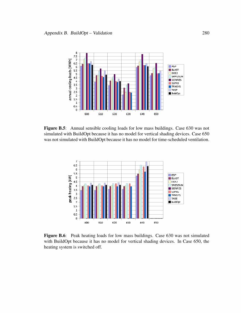
Appendix B. BuildOpt – Validation 280
Figure B.5: Annual sensible cooling loads for low mass buildings. Case 630 was notsimulated with BuildOpt because it has no model for vertical shading devices. Case 650was not simulated with BuildOpt because it has no model for time-scheduled ventilation.
Figure B.6: Peak heating loads for low mass buildings. Case 630 was not simulatedwith BuildOpt because it has no model for vertical shading devices. In Case 650, theheating system is switched off.

Appendix B. BuildOpt – Validation 281
Figure B.7: Annual peak sensible cooling loads for low mass buildings. Case 630was not simulated with BuildOpt because it has no model for vertical shading devices.Case 650 was not simulated with BuildOpt because it has no model for time-scheduledventilation.
Figure B.8: Annual heating loads for high mass buildings. Case 930 was not simulatedwith BuildOpt because it has no model for vertical shading devices. In Case 950, theheating system is switched off.
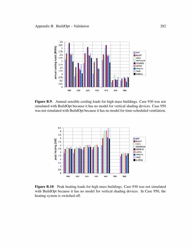
Appendix B. BuildOpt – Validation 282
Figure B.9: Annual sensible cooling loads for high mass buildings. Case 930 was notsimulated with BuildOpt because it has no model for vertical shading devices. Case 950was not simulated with BuildOpt because it has no model for time-scheduled ventilation.
Figure B.10: Peak heating loads for high mass buildings. Case 930 was not simulatedwith BuildOpt because it has no model for vertical shading devices. In Case 950, theheating system is switched off.

Appendix B. BuildOpt – Validation 283
Figure B.11: Annual peak sensible cooling loads for high mass buildings. Case 930was not simulated with BuildOpt because it has no model for vertical shading devices.Case 950 was not simulated with BuildOpt because it has no model for time-scheduledventilation.
Figure B.12: Sensitivity of annual heating load for low mass buildings. Case 630 wasnot simulated with BuildOpt because it has no model for vertical shading devices.

Appendix B. BuildOpt – Validation 284
Figure B.13: Sensitivity of annual sensible cooling load for low mass buildings. Case630 was not simulated with BuildOpt because it has no model for vertical shading de-vices. Case 650 was not simulated with BuildOpt because it has no model for time-scheduled ventilation.
Figure B.14: Sensitivity of peak heating load for low mass buildings. Case 630 was notsimulated with BuildOpt because it has no model for vertical shading devices.

Appendix B. BuildOpt – Validation 285
Figure B.15: Sensitivity of peak sensible cooling load for low mass buildings. Case 630was not simulated with BuildOpt because it has no model for vertical shading devices.Case 650 was not simulated with BuildOpt because it has no model for time-scheduledventilation.
Figure B.16: Sensitivity of annual heating load for high mass buildings. Case 930 wasnot simulated with BuildOpt because it has no model for vertical shading devices.

Appendix B. BuildOpt – Validation 286
Figure B.17: Sensitivity of annual sensible cooling load for high mass buildings. Case930 was not simulated with BuildOpt because it has no model for vertical shading de-vices. Case 950 was not simulated with BuildOpt because it has no model for time-scheduled ventilation.
Figure B.18: Sensitivity of peak heating load for high mass buildings. Case 930 wasnot simulated with BuildOpt because it has no model for vertical shading devices.

Appendix B. BuildOpt – Validation 287
Figure B.19: Sensitivity of peak sensible cooling load for high mass buildings. Case930 was not simulated with BuildOpt because it has no model for vertical shading de-vices. Case 950 was not simulated with BuildOpt because it has no model for time-scheduled ventilation.

Appendix B. BuildOpt – Validation 288
B.1.4.2 Indoor Air Temperatures
The minimum indoor air temperature computed by BuildOpt is for the low mass
test cases in the range of the results of the other tested programs, but it is for the high
mass test cases 1K lower. The average indoor air temperature computed by BuildOpt is
within the range of the results of the other tested programs. The maximum indoor air
temperature computed by BuildOpt is for the high mass test cases 3K lower and for the
low mass test cases 4K lower than the results of the other tested programs. Consequently,
for Case 900FF, there are fewer hours with a high indoor air temperature compared to the
other tested programs, but the number of hours with low indoor air temperature coincides
well with the results of the other tested programs (see Fig. B.23). On January 4, the
hourly free float temperature is in the range of results of the other tested programs for
both, the low mass test case (see Fig. B.24) and the high mass test case (see Fig. B.25).

Appendix B. BuildOpt – Validation 289
Figure B.20: Minimum hourly annual temperature for free-float test cases. Case 650FFwas not simulated with BuildOpt because it has no model for time-scheduled ventilation.Case 950FF was not simulated with BuildOpt because it has no model for time-scheduledventilation.
Figure B.21: Average hourly annual temperature for free-float test cases. Case 650FFwas not simulated with BuildOpt because it has no model for time-scheduled ventilation.Case 950FF was not simulated with BuildOpt because it has no model for time-scheduledventilation.
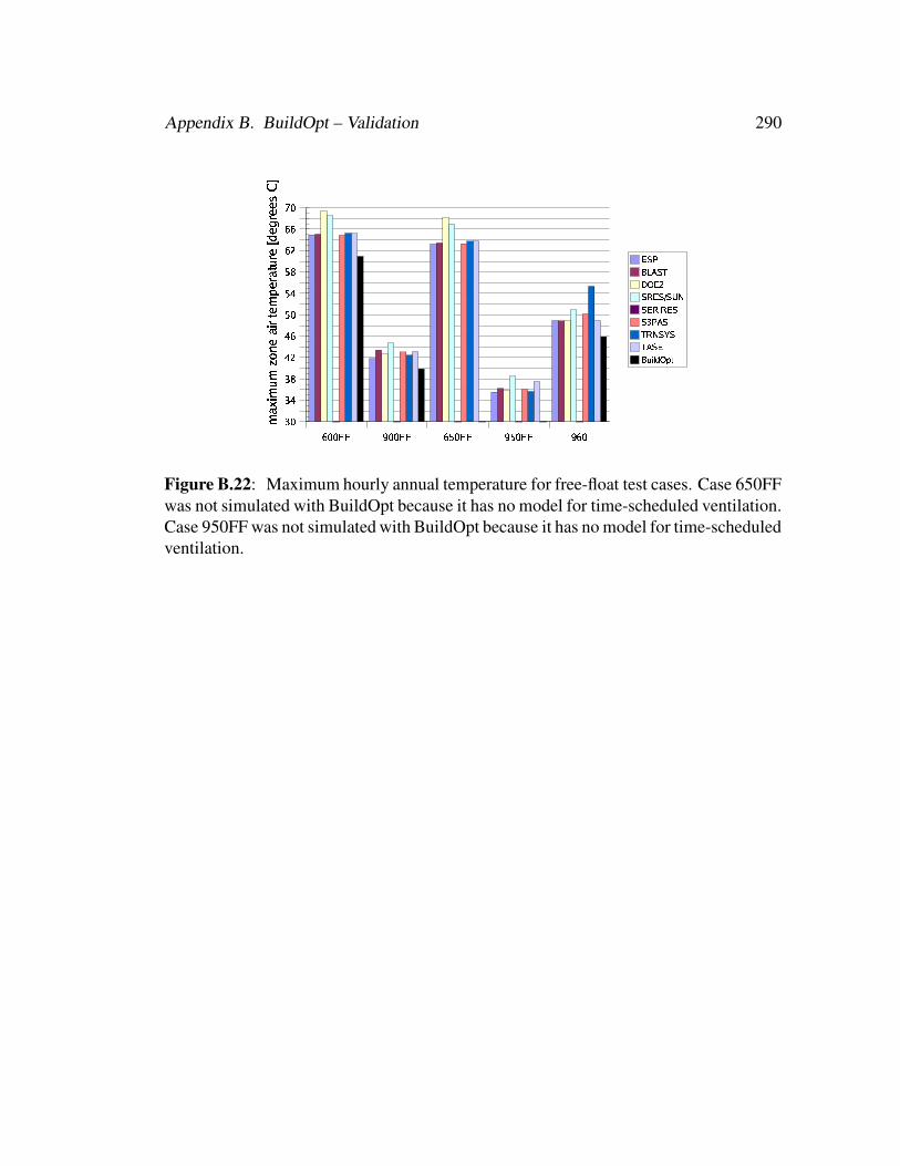
Appendix B. BuildOpt – Validation 290
Figure B.22: Maximum hourly annual temperature for free-float test cases. Case 650FFwas not simulated with BuildOpt because it has no model for time-scheduled ventilation.Case 950FF was not simulated with BuildOpt because it has no model for time-scheduledventilation.

Appendix B. BuildOpt – Validation 291
−10 0 10 20 30 400
50
100
150
200
250
300
350
400
450
500
temperature bins [° C]
hour
ly o
ccur
renc
e fo
r eac
h bi
n
ESPBLASTDOE2.1DSRES/SUNSERIRESS3PASTRNSYSTASEBuildOpt
Figure B.23: Annual hourly temperature frequency for each 1C bin for Case 900FF.
5 10 15 20
−15
−10
−5
0
5
10
15
20
25
30
35
time [h] of Jan. 4
Indo
or a
ir te
mpe
ratu
re, [
° C]
ESPBLASTDOE2.1DSRES/SUNS3PASTRNSYSTASEBuildOpt
Figure B.24: Hourly free float temperatures on January 4 for low mass building (Case600FF).

Appendix B. BuildOpt – Validation 292
5 10 15 20−6
−4
−2
0
2
4
6
8
10
time [h] of Jan. 4
Indo
or a
ir te
mpe
ratu
re, [
° C]
ESPBLASTDOE2.1DSRES/SUNS3PASTRNSYSTASEBuildOpt
Figure B.25: Hourly free float temperatures on January 4 for heavy mass building (Case900FF).

Appendix B. BuildOpt – Validation 293
B.1.4.3 Incident and Transmitted Solar Radiation
The annual incident and transmitted solar radiation computed by BuildOpt coin-
cides with the results of the other tested programs. However, on March 5 and July
27, which are cloudy days, BuildOpt’s hourly incident solar radiation on a south surface
is shifted by 1 hour compared to the results of the other tested programs (see Fig. B.29
and Fig. B.30). The values of BuildOpt are nearly symmetric to 12: 00, whereas the
values of the other tested programs are nearly symmetric to 13: 00. For this building
site, on March 5, 1990, the sun is highest at 12: 11, and on July 27, 1990, it is highest
at 12: 06 (neglecting daylight savings time).1 Thus, the solar radiation should nearly be
symmetric to 12: 00, as computed by BuildOpt, rather than to 13: 00, as computed by
the other tested programs.
Figure B.26: Annual incident solar radiation.
1See, for example, http://aa.usno.navy.mil/data/docs/RS_OneDay.html .

Appendix B. BuildOpt – Validation 294
Figure B.27: Annual transmitted solar radiation with unshaded windows.
Figure B.28: Annual transmitted solar radiation with shaded windows. Case 930 wasnot simulated with BuildOpt because it has no model for vertical shading devices.

Appendix B. BuildOpt – Validation 295
5 10 15 200
10
20
30
40
50
60
70
time [h] of March 5
Inci
dent
tota
l sol
ar ra
diat
ion,
Sou
th in
[W/m
2 ] ESPDOE2.1DSRES/SUNSERIRESS3PASTRNSYSTASEBuildOpt
Figure B.29: Hourly incident solar radiation on a cloudy day (March 5) on the southfacing surface.
5 10 15 200
50
100
150
200
250
300
350
400
450
time [h] of July 27
Inci
dent
tota
l sol
ar ra
diat
ion,
Sou
th in
[W/m
2 ] ESPDOE2.1DSRES/SUNSERIRESS3PASTRNSYSTASEBuildOpt
Figure B.30: Hourly incident solar radiation on a clear day (July 27) on the south facingsurface.

Appendix B. BuildOpt – Validation 296
5 10 15 200
10
20
30
40
50
60
70
time [h] of March 5
Inci
dent
tota
l sol
ar ra
diat
ion,
Wes
t in
[W/m
2 ] ESPDOE2.1DSRES/SUNSERIRESS3PASTRNSYSTASEBuildOpt
Figure B.31: Hourly incident solar radiation on a cloudy day (March 5) on the westfacing surface.
5 10 15 200
100
200
300
400
500
600
700
800
time [h] of July 27
Inci
dent
tota
l sol
ar ra
diat
ion,
Wes
t in
[W/m
2 ] ESPDOE2.1DSRES/SUNSERIRESS3PASTRNSYSTASEBuildOpt
Figure B.32: Hourly incident solar radiation on a clear day (July 27) on the west facingsurface.

Appendix B. BuildOpt – Validation 297
B.1.4.4 Solar Transmissivity and Shading Coefficients
The solar transmissivity and the shading coefficients computed by BuildOpt coincide
with the results of the other tested programs.
Figure B.33: Annual transmissivity coefficient of windows. This is the ratio betweenthe unshaded transmitted solar radiation and the incident solar radiation.
Figure B.34: Annual overhang and fin shading coefficients. The shading coefficientis defined as one minus the ratio between the shaded transmitted solar radiation andthe unshaded transmitted solar radiation. Case 930 was not simulated with BuildOptbecause it has no model for vertical shading devices.

Appendix B. BuildOpt – Validation 298
B.1.4.5 Hourly Heating and Cooling Power
The hourly heating and cooling power coincide with the results of the other tested
programs.
5 10 15 20
−3
−2
−1
0
1
2
3
4
time [h] of January 4
Hea
ting
(+) a
nd c
oolin
g (−
) loa
d in
[kW
]
ESPBLASTDOE2.1DSRES/SUNS3PASTRNSYSTASEBuildOpt (Heating)BuildOpt (Cooling)
Figure B.35: Hourly heating and cooling power on January 4 for low mass building(Case 600).
B.1.5 Conclusions
BuildOpt’s results coincide for most tests with the results of the other tested pro-
grams. The largest differences are for the high mass test cases. For these tests, the an-
nual cooling load and the annual peak cooling computed by BuildOpt is low compared
to the values of the other tested programs. Also, for the free floating cases, the maximum
and the minimum indoor air temperature computed by BuildOpt are low. However, the
differences are relatively small, and we do not think that they are caused by a modeling
error or a programming error.
Appendix B. BuildOpt – Validation 299
B.2 Daylighting Model
B.2.1 Introduction
For the validation of the daylighting model, we used the benchmark tests from
Laforgue (1997) and Fontoynont et al. (1999) that have been produced in the Task 21
of the International Energy Agency (IEA) Solar Heating & Cooling Program. These
benchmark tests compare the values of the daylight factors for rectangular room con-
figurations with increasing complexity. (The daylight factors are defined as the ratio
of the illuminance on indoor surfaces at specific locations to the simultaneous horizon-
tal illuminance on the roof.) The here presented daylight factors were obtained either
by measurement, by using analytical computations, or by using different commercially
available detailed daylighting simulation programs.
All test cases have a room aperture with no glass. Hence, for the daylight validation,
we set the light transmittance of the window to one for all incidence angles. However,
we remind that if a room has a window, then BuildOpt uses the same window model for
the daylight transmittance and for the solar transmittance, with possibly different input
data. This window model was validated in Section B.1.
Due to the model simplifications in BuildOpt’s daylighting model, we used only the
results for side-lit rooms with an isotropic sky, and we compared only daylight factors

Appendix B. BuildOpt – Validation 300
Side view
0.90
2.15
3.05
apertureframe
aperture
Top view
B E F
reference pointaperture
6.78
3.05
1.52
51.
525
1.74 2.70 1.70
Figure B.36: LESO scale model. The gray area in the left-hand figure shows thelocation of the aperture, and the black dots in the right-hand figure show the location ofthe daylight reference points.
on horizontal surfaces.
B.2.2 Specification of the Test Cases
B.2.2.1 LESO Scale Model
For the first set of test cases, we used data from the scale model of the Laboratoire
d’Energy Solaire (LESO) of the Ecole Polytechnique Federale de Lausanne (EPFL),
Switzerland. Fig. B.36 shows the scale model with the location of the daylight reference
points that we used in our validation. All daylight reference points are 0.75m above the
floor. Fontoynont et al. (1999) report that the frame of the aperture was not simulated
with any of the software. For the room and ground reflectance, we used the reflectance
values shown in Tab. B.2.2
2Laforgue (1997) lists in the test specification for cases (a) and (b) reflectance for all room surfacesand for the ground of 0.02, in contradiction to the values listed in the result tables, which are zero for allroom surfaces and for the ground. The difference between the results is small.

Appendix B. BuildOpt – Validation 301
case (a) case (b) case (c) case (d)Ceiling 0 0 0.83 0.83Walls 0 0 0.60 0.60Floor 0 0 0.28 0.28Ground 0 0.29 0 0.29
Table B.2: Reflectance values for the LESO scale model.
B.2.2.2 CSTB/ECAD Scale Model
For the second set of test cases, we used data from the scale model of the Centre
Scientifique du Batiment (CSTB), France. Fig. B.37 shows the scale model and the
location of the reference points that we used in our validation. We used the reflectance
values shown in Tab. B.3.3
case (a) and (b) case (c) and (d)Ceiling 0 0.70Walls 0 0.50Floor 0 0.30Ground 0 0.30
Table B.3: Reflectance values for the CSTB scale model.
For case (a), the daylight reference points were located on the floor and for case (b),
they were located 0.8m above the floor. For case (c), the daylight reference points were
for Genelux and BuildOpt on the floor, for SUPERLITE 0.08m above the floor, and at an
unspecified height for the CSTB sim results. For case (d), the daylight reference points
were 0.8m above the floor for all tabulated values.
3The ground reflectance is not specified in Laforgue (1997). However, from the daylight factors thatare tabulated in Laforgue (1997), one can conclude that for cases (a) and (b), the ground reflectance mustbe zero. For cases (c) and (d), the results in Laforgue (1997) were obtained by using a ground reflectanceof 0.30 (Carroll, 2003). This value accounted for the fact that the 1:10 scale model was placed on a 1mhigh table, and hence, the view factor to the sky was as in a room on the 4-th floor. Consequently, anobserver that looks downward from the ceiling may see part of the illuminated sky.

Appendix B. BuildOpt – Validation 302
Side view
1.0
1.5
0.5
3.0aperture
Top view
4 1
5 2
6 3
reference point
3.0 3.0 3.0
9.0
1.0
3.5
3.5
1.0
9.0
aperture
Figure B.37: CSTB scale model. The black dots in the top figure show the location ofthe daylight reference points, and the gray area in the bottom figure shows the locationof the aperture.

Appendix B. BuildOpt – Validation 303
B.2.3 Results
B.2.3.1 LESO Scale Model
Tab. B.4 and Fig. B.38 show the daylight factors for all benchmark tests for the LESO
scale model that we used in the BuildOpt validation. For the cases (a) and (b) in which
all room surfaces are non-reflecting, BuildOpt’s daylight factors are within the range of
the other results at the reference points E and F which are at a distant of 4.44m and
6.14m from the aperture. For the reference point B, which is at a distant of 1.74m from
the aperture, the daylight factor computed by BuildOpt is about 3.5% higher in absolute
value than the values listed in Laforgue (1997). For the cases (c) and (d), which used a
room with reflecting surfaces, the daylight factors at all reference points are within the
range of the other tabulated results. For the daylight reference points E and F, which are
far away from the aperture, the daylight factors computed by BuildOpt are on the lower
side compared to the other tabulated results. This is because with increasing distance
between daylight reference point and aperture, more of the daylight that arrives at the
reference point underwent multiple reflections. However, BuildOpt computes only the
first reflection, and consequently, it underestimates the daylight illuminance for locations
far away from the aperture.

Appendix B. BuildOpt – Validation 304
Case (a)Point EPFL scale SUPERLITE RADIANCE Genelux BuildOpt
B 8.11 8.86 6.39 9.42 11.09E 1.39 1.53 1.14 1.43 1.51F 0.68 0.69 0.53 0.80 0.65
Case (b)Point EPFL scale SUPERLITE RADIANCE Genelux BuildOpt
B 8.27 9.17 6.57 9.42 11.13E 1.34 1.57 1.26 1.43 1.53F 0.69 0.70 0.48 0.80 0.66
Case (c)Point EPFL scale SUPERLITE RADIANCE Genelux BuildOpt
B 12.13 11.5 8.44 10.54 11.96E 4.09 3.17 2.40 2.29 1.90F 3.12 2.21 1.46 1.48 1.18
Case (d)Point EPFL scale SUPERLITE RADIANCE Genelux BuildOpt
B 12.74 13.27 8.55 13.4 13.37E 4.24 3.90 2.38 3.56 2.50F 3.18 2.69 1.49 2.34 1.55
Table B.4: Daylight factors in [%] for the LESO scale model with an isotropic sky.

Appendix B. BuildOpt – Validation 305
(a) Reflectance inside 0%, ground 0%. (b) Reflectance inside 0%, ground 29%.
(c) Reflectance inside non-zero,ground 0%.
(d) Reflectance inside non-zero,ground 29%.
Figure B.38: Daylight factors for the LESO scale model with an isotropic sky.

Appendix B. BuildOpt – Validation 306
B.2.3.2 CSTB/ECAD Scale Model
Tab. B.5 and Fig. B.39 show the daylight factors for all benchmark tests for the LESO
scale model. For the cases (a) and (b) which used a room with black surfaces, BuildOpt’s
results are in the range of all other results except at the reference points 1 and 3, at which
the daylight factor computed by BuildOpt is 1% to 2% lower in absolute value. For cases
(c) and (d) that used a room with gray surfaces, BuildOpt underestimates the daylight
factor by 2% in absolute value for the reference points that are close to the aperture.
The accuracy is higher for reference points that are farther away from the aperture. In
general, BuildOpt tends to underestimate the daylight factors because it does not account
for multiple reflectances.

Appendix B. BuildOpt – Validation 307
(a) Reflectance inside 0%,ground 0%, reference points onfloor.
(b) Reflectance inside 0%,ground 0%, reference points 0.8mabove floor.
(c) Reflectance inside non-zero,ground 30%, reference points on floor.
(d) Reflectance inside non-zero,ground 30%, reference points 0.8mabove floor.
Figure B.39: Daylight factors for the CSTB/ECAD scale model with an isotropic sky.

Appendix B. BuildOpt – Validation 308
Case (a)Point analytic 1 CSTB sim Genelux BuildOpt
1 5.94 5.90 6.16 4.572 8.01 8.00 8.21 8.003 5.94 5.90 6.16 4.574 1.71 1.70 1.89 1.475 2.21 2.20 2.35 2.206 1.71 1.70 1.89 1.47
Case (b)Point analytic 2 RADIANCE Genelux BuildOpt
1 4.32 4.30 4.20 3.262 5.81 5.80 5.62 5.793 4.32 4.20 4.20 3.264 1.02 1.00 1.00 0.875 1.32 1.20 1.39 1.326 1.02 0.90 1.00 0.87
Case (c)Point CSTB sim Genelux SUPERLITE BuildOpt
1 7.20 8.00 7.93 6.222 9.30 9.30 9.44 8.383 7.20 8.00 7.93 6.224 3.00 3.40 3.03 2.305 3.50 3.40 3.42 2.836 3.00 3.30 3.03 2.30
Case (d)Point RADIANCE Genelux BuildOpt
1 7.00 5.64 4.962 8.50 6.95 6.033 6.90 5.69 4.964 2.30 1.84 1.615 2.80 2.35 1.876 2.40 1.87 1.61
Table B.5: Daylight factors in [%] for the CSTB/ECAD scale model with an isotropicsky.

Appendix B. BuildOpt – Validation 309
B.2.4 Conclusions
The daylight factors computed by BuildOpt coincide for most test cases with the
daylight factors that were obtained with other, substantially more detailed, commercial
daylighting programs or by using analytical formulas.
The largest differences between BuildOpt’s results and the values tabulated in the
IEA reports from Laforgue (1997) and Fontoynont et al. (1999) are for rooms with black
surfaces at reference points that are close to a wall. For these cases, BuildOpt underesti-
mates the daylight factor by 2% in absolute value.
For the more realistic cases in which the room has reflecting surfaces, the daylight
factors computed by BuildOpt are either within the range of the tabulated values, or
within an absolute difference of 1%.
For rooms with reflecting surfaces, BuildOpt tends to underestimate the daylight
factors at locations far away from the aperture because it does not take into account
multiple reflections.