simulation-based performance modeling of uml … · universita ca’ foscari di venezia`...
TRANSCRIPT

Universita Ca’ Foscari di Venezia
Dipartimento di InformaticaDottorato di Ricerca in Informatica
Ph.D. Thesis: TD-2004-1
Simulation-Based Performance Modeling ofUML Software Architectures
Moreno Marzolla
Supervisor
Prof. Simonetta Balsamo
February, 2004

Author’s Web Page: http://www.dsi.unive.it/˜marzolla
Author’s e-mail: [email protected]
Author’s address:
Dipartimento di InformaticaUniversita Ca’ Foscari di VeneziaVia Torino, 15530172 Venezia Mestre – Italiatel. +39 041 2348411fax. +39 041 2348419web: http://www.dsi.unive.it

Abstract
Quantitative analysis of software systems is being recognized as an important issuein the software development process. Performance analysis can help to addressquantitative system analysis from the early stages of the software development lifecycle, e.g, to compare design alternatives or to identify system bottlenecks. Earlyidentification of performance problems is desirable as the cost of design changeincreases with the later phases of the software development cycle.
This thesis addresses the problem of performance analysis of software systemsdescribed at a high level of detail. We adopt a model-based approach: starting froma software model, we derive a performance model which is then evaluated. This kindof approach has the advantage of being applicable since the early software develop-ment phases; in contrast, a measurement-based approach consisting on identifyingproblems by direct measurements on a running system can not.
We consider software descriptions as a set of annotated Unified Modeling Lan-guage (UML) diagrams. UML is a widely used notation for describing and specifyingsoftware artifacts, and recently it is being also considered for performance evalua-tion purposes. We define the performance model as a process-oriented simulationmodel. Simulation is a powerful modeling technique which can represent generaland unconstrained system models, so that the software model can be more accu-rately represented. An algorithm for translating UML software specifications intosimulation models is described. The proposed technique defines a set of annotationof UML specifications to add quantitative, performance-oriented informations. Theprofile is based on the UML profile for Schedulability, Performance and Time spec-ification. The system is described in term of Use Case, Activity and Deploymentdiagrams. Use Case diagrams correspond to workloads applied to the system. Ac-tivity diagrams provide a high-level description of the computation steps performedby the system, and Deployment diagrams describe the physical resources on whichthe computations take place. A process-oriented simulation model can then be au-tomatically derived from the annotated specification. Execution of the simulationprogram provides performance results that can be directly interpreted at the UMLsoftware specification level. The described algorithm has been implemented in a pro-totype tool called UML-Ψ (UML Performance SImulator), which is demonstratedon a case study to show the validity of the approach. The UML-Ψ tool is writtenin C++ and is based on a general-purpose process-oriented simulation library. It

parses annotated UML models, automatically builds the corresponding simulationmodel and executes it. Performance results are inserted into the original UML modelas tagged values, in order to give feedback to the user.

Sommario
L’analisi quantitativa di sistemi software viene riconosciuta come un aspetto im-portante nel processo di sviluppo del software. L’analisi quantitativa puo aiutare avalutarne le prestazioni a partire dai primi passi del ciclo di sviluppo, ad esempioconsentendo di confrontare differenti alternative o individuare colli di bottiglia nelsistema. L’individuazione precoce di problemi legati a scarse prestazioni e desider-abile, poiche il costo di cambiare il disegno del software cresce col progredire dellefasi di sviluppo.
Questa tesi affronta il problema dell’analisi delle prestazioni di sistemi softwaredescritti ad alto livello. Viene adottato un approccio basato su modelli: a partire daun modello del sistema software, viene descritto un modello di prestazione che e poivalutato. Un approccio di questo tipo ha il vantaggio di poter essere applicato findalle prime fasi del ciclo di sviluppo del software; al contrario, non possono essere ap-plicati durante le fasi iniziali gli approcci basati sulle misurazioni, perche consistononell’identificare problemi tramite misura diretta su un sistema in esecuzione.
Vengono considerate descrizioni di sistemi software espresse come un insieme didiagrammi UML annotati. UML e una notazione ampiamente utilizzata per la de-scrizione e la specifica di artefatti software, e recentemente e stata considerata anchenella valutazione di prestazioni. Definiremo un modello di prestazioni in termini diun modello di simulazione orientato a processi. La simulazione e una tecnica moltoespressiva con la quale e possibile rappresentare modelli generali e senza vincoli, talida poter rappresentare piu accuratamente il modello del software. Verra descritto unalgoritmo per la traduzione di specifiche UML annotate nel modello di simulazione.La tecnica proposta definisce un insieme di annotazioni di specifiche UML per ag-giungere informazioni quantitative orientate alle prestazioni. Il profilo e basato sul“ UML profile for Schedulability, Performance and Time Specification”. Il sistemaviene descritto in termini di diagrammi di caso d’uso, di attivita e di deployment.I diagrammi di caso d’uso corrispondono ai carichi di lavoro applicati al sistema.I diagrammi di attivita forniscono una descrizione ad alto livello dei passi di com-putazione effettuati dal sistema, e i diagrammi di deployment descrivono le risorsefisiche su cui le computazioni avvengono. A partire dalle specifiche annotate vienederivato un modello di simulazione orientato a processi. L’esecuzione del programmadi simulazione fornisce risultati di prestazioni che possono essere direttamente inter-pretati a livello di specifica UML. L’algoritmo proposto e stato implementato in un

prototipo chiamato UML-Ψ(UML Performance SImulator), che verra applicato adun caso di studio per mostrare la validita dell’approccio. UML-Ψ e scritto in C++ed e basato su una libreria di simulazione generica orientata a processi. UML-Ψlegge modelli UML annotati, costruisce automaticamente il corrispondente modellodi simulazione e lo esegue. Le misure di prestazione sono inserite nel modello UMLoriginale come tagged values, allo scopo di fornire un riscontro all’utente.

Acknowledgments
I would like to thank my advisor, Simonetta Balsamo, for her continuous supportand supervision in developing this research and the related publications.
This work has been carried out at the Dipartimento di Informatica, UniversitaCa’ Foscari di Venezia, Italy. I would like to thank all the personnel for their supportand for making the department a nice and friendly place for doing research. Inparticular, special thanks to my friends and colleagues: Chiara, Claudio, Damiano,Fabrizio, Marta, Matteo, Ombretta, Silvia (for many rotationally invariant ideas)and Valentino. Many thanks to all the people I met at schools and conferences,including Andrea (the ghost of unemployment is already knocking my door), Mimmoand Claudio. All my gratitude and friendship goes to Paolo who shared with methis three-years long adventure, and who hosted me many times in Florence andPisa; I wish you a good luck for all your future activities.
During my PhD I was initially supported by INFN (Istituto Nazionale di FisicaNucleare) Padova, Italy. Many thanks to my supervisors Roberto and Mauro, andthe many friends there: Alvise, Andrea L., Andrea P., Enrico, Federico, Fulvio,Marcello and Monica.
The work described in this thesis has been partially supported by research fundsprovided by MURST Research Project Sahara and by MIUR Project FIRB “Per-formance Evaluation of Complex Systems: Techniques, Methodologies and Tools”.
Finally, many thanks to my family for their enduring and constant support andencouragement: Gabriella, Gianni, Osvaldo, and also nonna Rina.


Contents
I Setting the Context 1
1 Introduction 31.1 Software Performance Evaluation . . . . . . . . . . . . . . . . . . . . 61.2 Previous work . . . . . . . . . . . . . . . . . . . . . . . . . . . . . . . 81.3 Contribution and outline of this thesis . . . . . . . . . . . . . . . . . 14
2 Introduction to UML 172.1 Use Case diagram . . . . . . . . . . . . . . . . . . . . . . . . . . . . . 182.2 Class diagram . . . . . . . . . . . . . . . . . . . . . . . . . . . . . . . 192.3 Interaction diagrams . . . . . . . . . . . . . . . . . . . . . . . . . . . 20
2.3.1 Sequence diagram . . . . . . . . . . . . . . . . . . . . . . . . . 202.3.2 Collaboration diagram . . . . . . . . . . . . . . . . . . . . . . 20
2.4 State diagram . . . . . . . . . . . . . . . . . . . . . . . . . . . . . . . 222.5 Activity diagram . . . . . . . . . . . . . . . . . . . . . . . . . . . . . 232.6 Deployment diagram . . . . . . . . . . . . . . . . . . . . . . . . . . . 232.7 Extension Mechanisms . . . . . . . . . . . . . . . . . . . . . . . . . . 24
3 Simulation 273.1 Introduction to Simulation . . . . . . . . . . . . . . . . . . . . . . . . 273.2 Advantages and Disadvantages of Simulation . . . . . . . . . . . . . . 283.3 Types of Systems . . . . . . . . . . . . . . . . . . . . . . . . . . . . . 293.4 Discrete-Event Simulation . . . . . . . . . . . . . . . . . . . . . . . . 293.5 Steps in a simulation study . . . . . . . . . . . . . . . . . . . . . . . . 34
II Description of the approach 37
4 Simulation modeling of UML 394.1 General Principles . . . . . . . . . . . . . . . . . . . . . . . . . . . . . 394.2 Overview of the approach . . . . . . . . . . . . . . . . . . . . . . . . 414.3 Overview of the Performance Model . . . . . . . . . . . . . . . . . . . 434.4 The Performance Model . . . . . . . . . . . . . . . . . . . . . . . . . 46
4.4.1 Performance Context . . . . . . . . . . . . . . . . . . . . . . . 474.4.2 Workload . . . . . . . . . . . . . . . . . . . . . . . . . . . . . 484.4.3 Association . . . . . . . . . . . . . . . . . . . . . . . . . . . . 494.4.4 OpenWorkload . . . . . . . . . . . . . . . . . . . . . . . . . . 494.4.5 ClosedWorkload . . . . . . . . . . . . . . . . . . . . . . . . . . 49

ii Contents
4.4.6 ActionBase . . . . . . . . . . . . . . . . . . . . . . . . . . . . 504.4.7 Transition . . . . . . . . . . . . . . . . . . . . . . . . . . . . . 504.4.8 CompositeAction . . . . . . . . . . . . . . . . . . . . . . . . . 514.4.9 SimpleAction . . . . . . . . . . . . . . . . . . . . . . . . . . . 514.4.10 JoinAction, ForkAction . . . . . . . . . . . . . . . . . . . . . . 524.4.11 Resource . . . . . . . . . . . . . . . . . . . . . . . . . . . . . . 524.4.12 Active Resource . . . . . . . . . . . . . . . . . . . . . . . . . . 524.4.13 Passive Resource . . . . . . . . . . . . . . . . . . . . . . . . . 534.4.14 ResActionBase . . . . . . . . . . . . . . . . . . . . . . . . . . 544.4.15 AcquireAction . . . . . . . . . . . . . . . . . . . . . . . . . . . 544.4.16 ReleaseAction . . . . . . . . . . . . . . . . . . . . . . . . . . . 55
4.5 Simulation Results . . . . . . . . . . . . . . . . . . . . . . . . . . . . 554.6 Differences with the UML Performance Profile . . . . . . . . . . . . . 56
5 Mapping Performance Model Elements to UML 595.1 The Performance Context . . . . . . . . . . . . . . . . . . . . . . . . 595.2 Modeling Workloads . . . . . . . . . . . . . . . . . . . . . . . . . . . 605.3 Modeling Resources . . . . . . . . . . . . . . . . . . . . . . . . . . . . 615.4 Modeling Scenarios . . . . . . . . . . . . . . . . . . . . . . . . . . . . 625.5 Tagged Value Types . . . . . . . . . . . . . . . . . . . . . . . . . . . 63
5.5.1 PAperfValue . . . . . . . . . . . . . . . . . . . . . . . . . . . . 645.5.2 RTarrivalPattern . . . . . . . . . . . . . . . . . . . . . . . . . 65
5.6 An Example . . . . . . . . . . . . . . . . . . . . . . . . . . . . . . . . 66
6 The Simulation Model 696.1 Mapping the UML Model into the Performance Model . . . . . . . . 69
6.1.1 Workloads . . . . . . . . . . . . . . . . . . . . . . . . . . . . . 726.1.2 Resources . . . . . . . . . . . . . . . . . . . . . . . . . . . . . 746.1.3 Actions . . . . . . . . . . . . . . . . . . . . . . . . . . . . . . 76
6.2 The validation issue . . . . . . . . . . . . . . . . . . . . . . . . . . . . 80
7 An application to UML Mobility Modeling 837.1 Introduction . . . . . . . . . . . . . . . . . . . . . . . . . . . . . . . . 837.2 The approach . . . . . . . . . . . . . . . . . . . . . . . . . . . . . . . 85
7.2.1 Modeling the choice of Mobility . . . . . . . . . . . . . . . . . 877.2.2 Modeling Mobility Behaviors . . . . . . . . . . . . . . . . . . . 887.2.3 Modeling Interactions between Components . . . . . . . . . . 89
7.3 Summary of the UML Mobility Approach . . . . . . . . . . . . . . . . 907.4 A Simple Example . . . . . . . . . . . . . . . . . . . . . . . . . . . . 91

Contents iii
III Implementation 93
8 libcppsim: A process-oriented simulation library 958.1 Introduction and general concepts . . . . . . . . . . . . . . . . . . . . 958.2 Coroutines . . . . . . . . . . . . . . . . . . . . . . . . . . . . . . . . . 968.3 Simulation processes . . . . . . . . . . . . . . . . . . . . . . . . . . . 1008.4 Sequencing Set implementations . . . . . . . . . . . . . . . . . . . . . 1018.5 Random variate generations . . . . . . . . . . . . . . . . . . . . . . . 1028.6 Output Data Analysis . . . . . . . . . . . . . . . . . . . . . . . . . . 108
9 UML-Ψ Tool Description 1159.1 Introduction . . . . . . . . . . . . . . . . . . . . . . . . . . . . . . . . 1159.2 UML-Ψ class diagram . . . . . . . . . . . . . . . . . . . . . . . . . . 1179.3 UML model representation . . . . . . . . . . . . . . . . . . . . . . . . 1179.4 Simulation model representation . . . . . . . . . . . . . . . . . . . . . 118
10 The NICE Case Study 12110.1 Introduction . . . . . . . . . . . . . . . . . . . . . . . . . . . . . . . . 12110.2 Equip Configuration Scenario . . . . . . . . . . . . . . . . . . . . . . 12210.3 Recovery Scenario . . . . . . . . . . . . . . . . . . . . . . . . . . . . . 12210.4 Simulation Modeling . . . . . . . . . . . . . . . . . . . . . . . . . . . 123
11 Conclusions 13111.1 Contributions of this work . . . . . . . . . . . . . . . . . . . . . . . . 13111.2 Relevant publications . . . . . . . . . . . . . . . . . . . . . . . . . . . 13311.3 Open Problems . . . . . . . . . . . . . . . . . . . . . . . . . . . . . . 134
Bibliography 137

iv Contents

List of Figures
1.1 Phases of the modeling and performance evaluation process . . . . . . 81.2 The modeling process proposed by Kahkipuro . . . . . . . . . . . . . 101.3 The PERMABASE modeling process . . . . . . . . . . . . . . . . . . 111.4 The modeling process proposed by Arief and Speirs . . . . . . . . . . 121.5 The modeling process proposed by De Miguel et al. . . . . . . . . . . 121.6 Performance simulation cycle proposed by Henning et al. . . . . . . . 13
2.1 A UML Sequence diagram . . . . . . . . . . . . . . . . . . . . . . . . 212.2 A UML Collaboration diagram . . . . . . . . . . . . . . . . . . . . . 212.3 A UML State diagram . . . . . . . . . . . . . . . . . . . . . . . . . . 222.4 A UML Activity diagram . . . . . . . . . . . . . . . . . . . . . . . . . 232.5 A UML Deployment diagram . . . . . . . . . . . . . . . . . . . . . . 24
3.1 Execution of a process-oriented simulation model . . . . . . . . . . . 313.2 Sequencing Set structure . . . . . . . . . . . . . . . . . . . . . . . . . 323.3 State transitions for a simulation process . . . . . . . . . . . . . . . . 343.4 Steps of a simulation modeling study . . . . . . . . . . . . . . . . . . 35
4.1 Performance modeling cycle . . . . . . . . . . . . . . . . . . . . . . . 414.2 Mapping UML elements into simulation processes . . . . . . . . . . . 434.3 Example of simulation model instance . . . . . . . . . . . . . . . . . . 454.4 Structure of the simulation performance model . . . . . . . . . . . . . 464.5 Open and Closed workloads . . . . . . . . . . . . . . . . . . . . . . . 484.6 The performance model from the UML Performance Profile . . . . . . 564.7 Associating different probabilities to incoming transitions . . . . . . . 57
5.1 UML representation of a Web video application. . . . . . . . . . . . . 67
6.1 Mapping open workloads into simulation processes . . . . . . . . . . . 726.2 Mapping closed workloads into simulation processes . . . . . . . . . . 736.3 Mapping active resources into simulation processes . . . . . . . . . . 746.4 Mapping passive resources into simulation processes . . . . . . . . . . 756.5 Mapping simple actions into simulation processes . . . . . . . . . . . 766.6 Mapping composite actions into a simulation process . . . . . . . . . 776.7 Mapping acquire actions into simulation processes . . . . . . . . . . . 786.8 Mapping release actions into simulation processes . . . . . . . . . . . 796.9 Mapping fork and join actions into simulation processes . . . . . . . . 80
7.1 Overview of the mobility modeling steps . . . . . . . . . . . . . . . . 86

vi List of Figures
7.2 A mobile user travels through three different LAN . . . . . . . . . . . 877.3 Deployment diagram for the example . . . . . . . . . . . . . . . . . . 887.4 UML representation of different mobility possibilities . . . . . . . . . 887.5 Activity diagrams associated to the mobility behaviors . . . . . . . . 887.6 Modeling nondeterministic and concurrent mobility behaviors . . . . 897.7 UML description of the interactions . . . . . . . . . . . . . . . . . . . 90
8.1 libcppsim package structure . . . . . . . . . . . . . . . . . . . . . . . 968.2 Example of flow control for routines and coroutines . . . . . . . . . . 978.3 libcppsim process package class diagram . . . . . . . . . . . . . . . . 1008.4 libcppsim Sequencing Set class diagram . . . . . . . . . . . . . . . . 1028.5 libcppsim Random Number Generators class diagram . . . . . . . . 1038.6 libcppsim statistics class diagram . . . . . . . . . . . . . . . . . . . 1098.7 Sample histogram printout . . . . . . . . . . . . . . . . . . . . . . . . 1138.8 Average waiting time of an M/M/1 queue . . . . . . . . . . . . . . . 114
9.1 The UML-Ψ model processing framework . . . . . . . . . . . . . . . . 1169.2 UML-Ψ class diagram, main part . . . . . . . . . . . . . . . . . . . . 1179.3 Class diagram for UML-Ψ simulation actions . . . . . . . . . . . . . . 1189.4 Class diagram for UML-Ψ simulation workloads . . . . . . . . . . . . 1199.5 Class diagram for UML-Ψ simulation resources . . . . . . . . . . . . . 119
10.1 NICE static software description . . . . . . . . . . . . . . . . . . . . . 12210.2 NICE configuration and recovery scenarios . . . . . . . . . . . . . . . 12310.3 Mean execution times . . . . . . . . . . . . . . . . . . . . . . . . . . . 12410.4 Activity diagram for the NICE case study . . . . . . . . . . . . . . . 12510.5 Structure of the simulation model . . . . . . . . . . . . . . . . . . . . 12710.6 Graph of the execution times from Table 10.1 . . . . . . . . . . . . . 128

List of Tables
4.1 List of processes in the simulation model . . . . . . . . . . . . . . . . 44
7.1 Simulation Parameters for the Mobile System Example . . . . . . . . 927.2 Simulation Results for the Mobile System Example. . . . . . . . . . . 92
10.1 Results for the NICE case study . . . . . . . . . . . . . . . . . . . . . 126

viii List of Tables

Acronyms
ADL Architectural Description Language
AQN Augmented Queuing Network
EQN Extended Queuing Network
FEL Future Event List
GSPN Generalized Stochastic Petri Nets
LQN Layered Queuing Network
NICE Naval Integrated Communication Environment
OMG Object Management Group
OS Operating System
QN Queuing Network
SA Software Architecture
SPA Stochastic Process Algebra
SPE Software Performance Engineering
SQS Sequencing Set
TVL Tag Value Language
UML Unified Modeling Language
XMI XML Metadata Interchange
XML Extensible Markup Language
XSLT Extensible Stylesheet Language Transformation

x List of Tables

ISetting the Context


1Introduction
Developing a complex software system is a challenging task, requiring resources interm of time and manpower to be accomplished. It is therefore very important thatthe system, once built, satisfies its functional and non functional requirements.
In recent years it has been recognized that the software development processesshould be supported by a suitable mechanism for early assessment of software per-formance. Early identification of unsatisfactory performance of Software Architec-ture (SA) can greatly reduce the cost of design change [91, 92]. The reason is thatcorrecting a design flaw is more expensive the later the change is applied during thesoftware development process. This is particularly true if a waterfall-style model [93]of software development is employed, as any change requires the development pro-cess to start back from the beginning. However, this is still a relevant issue whenevera different software development process is used.
Both quantitative and qualitative analysis can be performed at the softwarearchitectural design level. Qualitative analysis deals with functional properties of thesoftware system such as deadlock-freedom or security. Qualitative analysis is carriedout by measurement or by modeling the software system to derive quantitativefigures of merit, such as, for example, the execution profile of the software, memoryutilization or network utilization.
It should be noted that software performance modeling is challenging for differentreasons. First, it is difficult to derive meaningful performance measures from a staticanalysis of the code. The reason is that software performances heavily dependon the hardware platform on which the software executes, and also on the usagepattern the software is subject to. Moreover, software performance modeling cannot be performed on one component at a time, as critical issues may arise only whendifferent components interact.
We focus on models of software systems at the SA level. Many performancemodels have been proposed in the literature; these models include Queuing Net-work [57] and their various extensions (as Layered Queuing Network, which havebeen specifically developed to model client-server communication patterns in dis-tributed systems [38, 86, 103]), Stochastic Petri Nets [69] and Stochastic ProcessAlgebra [50]. At the moment there is no clear consensus on which model should bepreferred in practice. The general understanding is that different models are suit-

4 1. Introduction
able for different architectural styles and/or application domains. It is interestingto observe that most of the software performance evaluation approaches proposedso far are based on analytical models. This is motivated by the fact that these mod-els are well studied and understood. Also, these models can sometimes be solvedanalytically, providing performance results which are both exact and optionally canbe expressed parametrically with respect to one or more variables. This, however,comes at a price.
Analytical models which can be solved exactly can be derived only by imposingsome limitations on the SA from which they are derived. For example, Queuing Net-work (QN) models have a so-called product-form solution, which can be efficientlycomputed, only for special classes of networks. These produce-form models are con-strained both on their topology and on the distributions of jobs interarrival andservice times, which are often assumed to be exponentially distributed [28]. Hence,the hypothetical software system from which they are derived is constrained to beingmodeled only under the exponential distributions assumption. Even when solvableanalytical models can be derived, their size can grow exponentially with the size ofthe corresponding SA, making the performances model impossible to handle [7].
Analytical performance models can be structurally very different from the SAfrom which they are derived. This makes it very difficult to report performanceresults from the performance model to the original SA. This is very limiting, as soft-ware performance evaluation is supposed to provide the modeler with an immediatefeedback about possible performance problems.
There exist partial solutions to these problems. Approximate numerical tech-niques are available in many cases where product-form solutions do not exist [28].Unfortunately, those techniques themselves are subject to constraints in order to beapplied. They do not provide closed form solutions, which would be very useful inorder to study figures of merit as a function of some unknown parameter. Finally,many approximate techniques do not provide any error estimation on their results,meaning that it is impossible to quantify whether the computed values are goodapproximations of the exact results or not.
We address these limitations by developing a simulation model of SA. Simu-lation is a powerful modeling technique that allows general system models, thatis simulation models can represent arbitrarily complex real-world situations, whichcan be too complex or even impossible to represent by analytical models. Exam-ples of complex systems are computer systems with asynchronous communications,fork and join and simultaneous resource possessions, for which analytical models of-ten become difficult to analyze. We propose an approach for software performanceanalysis based on simulation to take advantage of this modeling technique.
Once the performance model has been chosen, one more problem remains: it isnecessary to choose a notation to use for describing software systems. Existing ap-proaches can be divided in two categories: the first deal with creating special-purposenotations for expressing both architectural features and performance informations;the second deals with building performance models from already existing design

5
formalisms.Examples in the first category (special-purpose notations for both architectural
and performance-oriented models) include the SPE approach by Smith, and Smithand Williams [91, 92, 102]. SPE is a comprehensive approach integrating perfor-mance analysis into the software development process. The software execution modelis represented by Execution Graphs, while the system model is based on QN andrepresents the physical resources on which the software executes.
Examples in the second category (performance models derived by software spec-ification notations already in use) include SDL [21] and LOTOS [29]. SDL is usedfor the specification of real-time systems; LOTOS is the CCITT recommended pro-tocol specification language. Both have been used for deriving various kinds ofperformance models (see [79] for references).
The problem with all those approaches is that both domain-specific and com-pletely new notations are unlikely to gain wide acceptance among the software en-gineering community. In recent years, the Unified Modeling Language [74, 87, 88] isemerging as a de facto standard for the high-level specification of software systemsand business processes, with particular emphasis of Object-oriented features. UMLis based on a graphical notation for specifying software artifacts; the notation isquite rich, including different kind of diagrams which can be used to model differentpoint of views of the system. An introduction to UML will be given in Chapter 2.
It comes at no surprise that the software performance community is looking withgreat interest toward using UML as the preferred software specification language.Unfortunately, this choice has some drawbacks. The main problem is that UMLis not a formal language. It lacks any formal semantics, and is only intuitivelyspecified [85]; this makes reasoning on UML specifications troublesome. Efforts areongoing to provide a precise specification of at least some subset of UML [81].
However, the fact that UML is informally specified does not mean that it hasno semantics at all. It is still possible to reason on UML specifications by takinginto account their intuitive (and widely agreed on) meaning. We propose a mappingbetween annotated UML specifications into process-oriented simulation models. Themapping will be described in detail in Part II, and is consistent with the intuitivesemantics of the UML diagrams considered. Moreover, the UML profile we definein Chapter 5 enforces an additional, informally specified semantics of UML usecase, activity and deployment diagrams corresponding to that of the performancemodel generated from them. This is exactly what a UML profile is supposed to beused for [74]. We are then considering UML specifications representing a dynamicbehavior described more precisely by their corresponding simulation models.
We consider quantitative evaluation of the performances of SA at the designlevel based on simulation models. We use SA specifications expressed in terms ofUML [74] diagrams. We propose to annotate the UML diagrams using a subset ofannotations defined in the UML Profile for Schedulability, Performance and TimeSpecification [75] (hereafter referred as UML performance profile). We define a sim-ulation model of an UML software architecture specification introducing an almost

6 1. Introduction
one-to-one correspondence between behaviors expressed in the UML model and theentities or processes in the simulation model.
The advantage of the proposed approach is twofold. First, this correspondencebetween the system and the model helps the feedback process to report performanceresults obtained by simulation back into the original SA. Second, this allow to definea simple translation algorithm from the SA to the simulation performance modelthat can be fully automated.
1.1 Software Performance Evaluation
Performance analysis of software systems can be carried out by measurement or bymodeling techniques. Direct measurement of an actual implementation provides anaccurate assessment of the performance of a software system. This is relatively easyto do, but requires to build a system implementation before the measurement cantake place. Implementing a complex system is usually a time-consuming, error-proneand expensive task; mastering this complexity is the goal of all the software devel-opment processes which have been proposed in the literature. We focus on softwaresystem at the SA design level. When SA exhibits performance-related problems, itis unlikely that such problems will be fixed once the architecture has been deployed,given the high costs associated with changing the design. Hence it is useful or evennecessary to evaluate early performance measures at the architectural design level,by developing and evaluating a model of SA. Performance model evaluation can isobtained by analytical, simulative or hybrid techniques.
Most of the research in the area of Software Performance Engineering (SPE) isbased on developing analytical models of SA [9, 15]. However, such models canusually be built only by imposing some structural restrictions on the original sys-tem model, depending on the specific modeling formalism which has been chosen;the reason is that analytical models have often a limited expressiveness. While itis sometimes possible to simplify the model of the system in order to make it an-alytically tractable, there are many cases in which the significant aspects of thesystem can not be effectively represented into the performance model. Examplesare concurrency, simultaneous resource possession and fork and join systems.
For these reasons we propose a software performance evaluation approach basedon simulation models. Simulation models can be arbitrarily detailed, in that, infor-mally, they impose no restrictions on what they can model. The analyst has themaximum degree of freedom in selecting the aspects of the real system, that is theSA in our context, to model, and at which level of detail. This freedom comes atsome cost: the drawback of simulation is that very complex models may require alot of time and computational resources in order to be executed. The results alsorequire sophisticated statistical techniques in order to be correctly understood [55].While it is true that any given system can be represented at an arbitrarily high levelof detail by a simulation model, the analyst often ignores the exact inner working of

1.1. Software Performance Evaluation 7
the system being simulated. This is certainly the case with SA, since they are definedat a high level of abstraction, and many details are postponed until the implementa-tion phase. However, while the software architect may ignore the inner details of thesystem being designed, he could have some more or less detailed knowledge of partof the architecture (for example if some pieces are taken from an existing, alreadyimplemented system). Whenever additional informations are available, they shouldbe used to obtain better and more realistic performance measures.
In order to easily apply SPE techniques it is convenient to refer to a commonnotation for software specification. Many notations are design-oriented and do notprovide built-in facilities to express informations necessary to derive a performancemodel. Two main approaches have been employed to overcome this limitation. Thefirst is the introduction of performance-oriented formalisms applied as informationsspecifically added to software models [91]. The second is the extension of modelinglanguages with additional notations [22, 52, 67]. While both approaches producedencouraging results, they are not widespread since they require software engineersto learn new and non-standard modeling formalisms and notations.
After its adoption in 1997 as an official Object Management Group (OMG) stan-dard, UML gained wide acceptance among software engineers thanks to its flexibilityand ease of use. UML is a language for specifying, visualizing, constructing, and doc-umenting software and non-software systems. It is particularly useful for, althoughnot limited to, designing Object-Oriented systems. UML provides users with a vi-sual modeling notation to develop and exchange models, and it defines extensibilityand specialization mechanisms. It supports specifications which are independentfrom the particular programming language and development process. Moreover,it supports higher-level development concepts such as components, collaborations,frameworks and patterns.
Given its wide acceptance, many software engineers are already acquainted withat least the basics of the UML notation. For this reason several recent SPE ap-proaches consider UML as a starting notation on which existing and new perfor-mance evaluation techniques can be applied. This can be done because UML pro-vides extension mechanisms to add new concepts and notations for those situationswhich are not covered by the core language, and to specialize the concepts, notation,and constraints for particular application domains.
We consider the performance-oriented modeling process illustrated in Fig. 1.1.The starting point is a description of the SA. We consider a description as a setof UML diagrams annotated with quantitative informations in order to derive asimulation-based performance model. The model is obtained using a suitable Mod-eling Algorithm and then implemented in a simulation program, which is eventuallyexecuted. Simulation results are a set of performance measures that can be used toprovide a feedback at the original SA design level. The feedback should pinpointperformance problems on the SA, and possibly provide suggestions to the softwaredesigner about how the problem can be solved. The modeling cycle shown in Fig. 1.1can be iterated until a SA with satisfactory performance is developed.

8 1. Introduction
DiagramsUML
Scenarios
ArchitectureSoftware
Model
Feedback
Impl.Model
Modeling Algorithm
Performance
PerformanceMeasures
ModelEvaluation
Evaluation ToolPerformance
ImplementationProgram
Model
Figure 1.1: Phases of the modeling and performance evaluation process
1.2 Previous work
Several approaches have been proposed on deriving performance models from archi-tectural specifications. Since recent approaches (including our proposal) use UMLas the notation for describing SA, we now briefly review some relevant works dealingwith performance evaluation of UML SA. As we will see shortly, most of them pro-pose the derivation of analytical performance models, while simulation models havebeen only recently considered in this field. Detailed considerations about analyticalperformance models for SA are outside the scope of this work. The interested readeris referred to [9, 15] for additional references and a thorough discussion covering awider spectrum of approaches. More informations can also be found in [53].
Approaches deriving analytic models
King and Pooley [56] propose a method for deriving performance models basedon Generalized Stochastic Petri Nets (GSPN) [69] from UML collaboration andstatechart diagrams. They propose to use a combination of UML diagrams – statediagrams embedded into collaboration diagrams – to better express the global stateof a system.
In [79], Pooley and King describe how the various kinds of UML diagrams can beused for performance evaluation purposes. Namely, they identify Actors in Use Casediagrams with workloads applied to the system. Implementation diagrams (Deploy-ment diagrams) are mapped on a queuing network model, representing the compu-tational resources (service centers in the QN) and communication links (queues inthe QN). Sequence diagrams can be used as traces to drive a simulation program.Finally, they suggest modeling of UML State diagrams using Markovian models.To demonstrate their approach, a queuing network model is derived from a UML

1.2. Previous work 9
description of an ATM system. The approach adds textual notations to UML dia-grams to include useful information for performance evaluation (e.g., time labels insequence diagrams). Such annotations are used to produce more complete models ofsoftware systems. It should be noted that their approach, in general, can be appliedregardless of the particular performance model derived.
In [23], Bernardi et al. derive a GSPN model from UML state and sequence dia-grams. They define two levels of modeling: a class level and an instance level. Theclass level is represented by state diagrams, and is used to describe the behavior ofsingle entities of a system. The instance level uses sequence diagrams to show pat-terns of interaction among objects (instances of classes). The GSPN model is thencreated merging together the information provided by the two kinds of diagrams.
Cortellessa and Mirandola [33] present an approach for translating UML se-quence diagrams, use case diagrams and deployment diagrams into performancemodel based on Extended Queuing Network (EQN) [59], using an intermediatetransformation into Execution Graphs [91]. System performance evaluation is pre-sented as an incremental process integrated in the software development life cycle,by using information of different kinds of UML diagrams from the early stages of thedevelopment process. The level of detail of the model is extended as the softwaredevelopment proceeds. This allows incremental building of a performance model ofthe system, which can be used to improve or modify the SA. The UML diagrams areannotated with quantitative informations, which are necessary to set the parame-ters of the model. Actors are annotated with the frequency they may appear in thesystem. Associations between actors and use cases are annotated with the proba-bilities that each actor executes each use case. Sequence diagrams are annotatedwith timing informations attached to events, and messages sent among objects aretagged with their sizes. Deployment diagrams represent various kinds of resources,and are annotated with suitable parameters such as bandwidth for network links,or speed of computational resources. Finally the three types of UML diagrams (usecase, sequence and deployment diagrams) are used together to build a EQN model.
In [43], Gomaa and Menasce use UML diagrams to represent the interconnectionpattern of a distributed software architecture. class diagrams are used to illustratethe static view of a system, while collaboration diagrams show the dynamic behavior.collaboration diagrams are extended with new elements showing interconnectionsand communication ports, and are added with performance annotations written inExtensible Markup Language (XML). Such annotations refer to routing probabilitybetween objects, average message processing time, average message size and averagearrival rate of requests. Then they derive a performance model based on QN.
Gu and Petriu [45] and Petriu and Shen [77] derive performance models basedon Layered Queuing Network (LQN) models [86] from a description of SA. Theyuse UML activity diagrams, annotated as defined in the UML Performance Profile.Diagrams and annotations are saved in XML files in the XML Metadata Interchange

10 1. Introduction
(XMI) format [76] and then translated in LQN models through Extensible StylesheetLanguage Transformation (XSLT) [104].
Lindemann et al. [63] develop an algorithm for deriving performance modelsbased on Generalized Semi-Markov Processes from UML state and activity diagrams.These diagrams are annotated with exponentially distributed or deterministic delaysapplied to events, and timed events trigger a state transition. Annotations are basedon an extension the UML Performance Profile.
Kahkipuro [54] proposes a framework on UML notation for describing perfor-mance models of component-based distributed systems. The performance modelis based on Augmented Queuing Network (AQN). The approach works as follows.UML diagrams are first converted into a textual notation called Performance Model-ing Language (PML). Then the PML performance model is translated into an AQN,which is then solved with approximate techniques. The results obtained from theAQN model are subsequently propagated to the PML model and finally to the soft-ware architectural model. The entire SA performance evaluation cycle is representedin Fig. 1.2.
UML Representation
PML Representation
AQN Representation AQN Results
PML Results
UML Results
Figure 1.2: The modeling process proposed by Kahkipuro [54]
The PERformance Modelling for Atm Based Applications and SErvices (PER-MABASE) project [98] deals with the automatic generation of performance modelsfrom software systems specified in UML. The software system is described in termof the following specifications:
• Workload specification: a description of the workloads driving the system;
• Application specification: a description of the behavior of the software system;
• Execution environment specification: this includes the description of physicalenvironment, including processors, network links and other resources;
• System scenario specification: the specification of a particular system instance,describing the configuration of the system (which components are presents andhow they are connected).

1.2. Previous work 11
UML is used to specify the workloads, the application behavior and the executionenvironment. The descriptions above are translated into a Composite Model DataStructure (CMDS) which can be checked for inconsistencies and refined if necessary.The CMDS is then translated into a performance model, whose execution providesfeedback which is reported back into the CMDS. The cycle is represented in Fig. 1.3.
Workload Specification
Application Specification
Execution Environment Specification
System ScenarioSpecification
CMDS
Transformations
Performance Model
Feedback
Figure 1.3: The PERMABASE modeling and performance evaluation process [98]
Hoeben [51] describes how UML diagrams can be used for performance evalua-tion. The approach uses UML class and component diagrams to represent informa-tions used for modeling the system dynamics. Sequence and collaboration diagramsare used to model the behavior of the system, and deployment diagrams representprocessors and network connections in the system. The performance model derivedfrom the combination of the diagrams is based on QN.
Approaches deriving simulation models
There currently are only a few works which derive simulation-based performancemodels from software systems. They are briefly described in this section.
Arief and Speirs [3, 4, 5, 6] develop an automatic tool for deriving simulationmodels from UML class and sequence diagrams. Their approach (see Fig. 1.4)consists on transforming the UML diagrams into a simulation model described asan XML document. The XML notation used to describe the simulation model hasbeen called SimML (Simulation Modeling Language). This model is then translatedinto a simulation program, which can be executed and provides performance results.What makes this approach particularly interesting is that the simulation modelis decoupled from its implementation. This makes it possible to implement thesimulation model using different languages. The authors developed two differentback-ends for translating the SimML model into simulation programs written inC++Sim [66] and JavaSim [65].
De Miguel et al. [36] introduce UML extensions for the representation and auto-matic evaluation of temporal requirements and resource usage, particularly targeted

12 1. Introduction
UML DesignNotation
Front-end GUI Tool
Back-end SimML Parser
SimulationProgram
SimML Notation
Figure 1.4: The modeling process proposed by Arief and Speirs [6]
at real-time systems. Their proposed performance evaluation sequence is depictedin Fig. 1.5.
ArchitecturalModel Construction UML Model
SimulationConfiguration
ConfigurationModel
Simulation Model
Generation
SimulationModel
SimulationExecution
SimulationResults
EvaluationConfiguration
1 2
3
4
5
Figure 1.5: The modeling process proposed by De Miguel et al. [36]
Step 1 deals with the construction of the architectural model of the system tobe analyzed; this is done by a UML CASE tool. UML elements are annotated withstereotypes, tagged values and stereotyped constraints in order to provide parame-ters to the simulation step. An XMI representation of the UML model is exportedand used in the next phases. Step 2 deals with the configuration of the simulation;given that the UML model might contain different alternative scenarios and alterna-tive behavioral specifications for the same elements, during this phase it is possibleto choose which scenarios and which behaviors to execute. Step 3 deals with theconfiguration of the simulation parameters, such as the statistics to collect, whichfilters to apply to simulation results, and the length of the simulation period. Step4 is the generation of the OPNET simulation model, which is executed during step5. Simulation results are finally displayed using OPNET facilities, and may pro-

1.2. Previous work 13
vide hints to reconfigure the UML architecture or used as criteria for architectureselection.
Hennig et al. [47, 49] describe a UML-based simulation framework for earlyperformance assessment of software/hardware systems described as UML Sequenceand Deployment diagrams. The framework follows the design-evaluation-feedbackcycle depicted in Fig. 1.6.
UML Model
XML experimentdescription
Simulator
OMNet++Core
SPEExtension
Statistics
NetworkTopology
Users andSystem Behavior
Pre-Modelledcomponents
Result(feedback)
Converter
Figure 1.6: The performance simulation cycle proposed by Hennig et al. [49]
The simulation cycle starts from a collection of UML diagrams, from which asubset (the gray boxes in the picture) is extracted and compiled into an XML docu-ment describing the simulation experiment. The UML diagrams which are extractedare Deployment diagrams, used to describe the physical environment on which thesoftware system executes, and Collaboration diagrams used to model the workloadapplied to the system and the internal behavior of the application being modeled.The converter module generates code for the network and behavior components ofthe simulator. The simulator itself is based on the discrete event simulation packageOMNet++ [96]. It contains core modules and specific SPE extensions (scheduler,workflow execution engine) as well as pre-modelled components. The statistics ofperformance observations collected during the execution of the simulator can be fedback into the original UML model as tagged values. The same approach is usedin [48] for the automatic generation of small components emulating the behavior ofreal one.

14 1. Introduction
1.3 Contribution and outline of this thesis
This work deals with automatic generation of simulation performance models fromhigh-level UML descriptions of SA. To the best of our knowledge, this is one of thefew approaches considering UML diagrams annotated with (a subset of) the UMLPerformance Profile [75]; the other we are aware of is a work by Petriu and Shen [77]in which the authors describe a graph-grammar derivation of performance modelsbased on LQN specifications from annotated UML models. The reason why theUML Performance Profile has not been widely considered yet is probably that ithas been released only very recently; we expect many other approaches along thisdirection in the future.
Motivating the use of UML We have already seen the advantages of using UMLas a notation for description of software systems. It is widely used and accepted inthe Software Engineering community, provides a set of diagrams allowing users torepresent a system from different point of views and at different level of details, andthere are many tools able to create and manipulate UML models. The drawback ofthe approach is that UML is only informally defined, so that software modelers mayuse different diagrams for the same purpose, or use the same notation with differentimplicit meaning. While addressing this limitation is outside the scope of this work(among others, the Precise UML group [81] is specifically working on this issue),the performance-oriented UML profile we will define in Chapter 5 actually enforcesan (operational) semantics of UML in terms of the derived performance model.Intuitively, we define the dynamic behavior of a set of annotated UML diagrams interms of the behavior of the implementation of the automatically derived simulationmodel.
Motivating the use of simulation model We chose to derive a simulationperformance model for different reasons, which have in part already been introducedin the previous discussion.
The main reason is that simulation models allow for unconstrained representa-tions of software models. This means that the performance model captures, and isable to analyze, all behaviors of the software under study. This is not always easyto do with analytical models. For example, in QN models it is difficult to handlesituations arising from finite capacity of queues (and subsequent blocking behav-ior); only approximate techniques can be used in some cases, and simulation is theonly approach in general [14]. Other difficulties arise when analyzing simultaneousresource possession, fork and join systems, synchronous vs asynchronous communi-cations, and many queuing disciplines (especially with complex priorities betweenrequests).
A direct consequence of using simulation is that deriving the performance modelfrom the software specification is very easy, as we will see in detail in Chapter 6.

1.3. Contribution and outline of this thesis 15
We define an almost one-to-one mapping between UML elements and simulationprocesses. The result is that the structure of the simulation model is very similarto the structure of the software model; this can be seen by the class diagram ofthe UML-Ψ tool described in Chapter 9. Direct translation of software model intoperformance model not only makes the modeling process easier and less error-prone,but allows an easier interpretation of the performance results back at the SA level.This is very important, as it is obvious that all indices computed by the performancemodel must be reported back at the design level, where the software modeler candecide whether the proposed SA fulfills its performance goals. This step, labeled asfeedback in the schema of Fig. 1.1, p. 8, is not trivial when the performance modelhas been obtained by applying a complex transformation to the software model.Reversing this transformation may be feasible only in special circumstances, meaningthat the software architect discovers a performance problem but is unable to identifythe specific component (or set of components) responsible for that misbehavior.
Motivating the use of process-oriented simulation As we will see in Chap-ter 3, there are different types of simulation models. The relevant ones for thisapplication are event-oriented and process-oriented simulation models. In event-oriented simulations the user must specify the different types of events which mayhappen, an event being defined as an instantaneous action taking no (simulation)time to execute, and causing a change in the system’s status. In a process-orientedsimulation, the user defines a set of simulation processes, each containing a set ofactions to be performed. Some of these actions may require some (simulated) timeto execute, while others may be instantaneous. We decided to implement the soft-ware performance model as a process-oriented simulation. In general, event-orientedsimulations are preferred when the number of event types to be modeled is relativelylow [17]. In contrast, the performance model derived from SA can be more easilydescribed as a set of interacting processes, each one with an internal behavior whichcan be procedurally described. Process-oriented simulations are well suited for thispurpose.
Contribution The contribution of this work is threefold. First we define aprocess-oriented simulation model for evaluating performances of SA at early de-velopment stage. Then, we propose a UML profile, based on the UML PerformanceProfile, providing facilities for
• Associating performance-oriented, quantitative annotations to UML elements;
• Specifying parameters to be used for the execution of the simulation perfor-mance model;
• Providing feedback to the software architect about the performance resultsfound by running the simulation.

16 1. Introduction
Finally, we show an actual software performance evaluation tool called called UML-Ψ (UML Performance SImulator). UML-Ψ automatically derives a simulation modelfrom annotated UML specifications, executes the model and provides results at theSA design level.
This thesis is divided in four main parts:
• In Part I we introduce the problem of software performance evaluation atthe architectural level. In Chapter 2 we given an introduction to the UMLnotation, and in Chapter 3 we introduce the basic concepts of discrete-eventsimulation modeling.
• In Part II we describe the structure of the simulation model and the profilefor annotating UML elements. Chapter 4 introduces the performance modelwhich will be used to represent the dynamic behavior of software systems.In Chapter 5 we show how concepts from the performance domain are im-plemented into UML models by means of an UML profile. In Chapter 6 wedescribe the simulation model in detail, including detailing the behavior of allsimulation processes involved. The performance evaluation technique will beextended in Chapter 7 to an integrated UML-based performance and mobilitymodeling approach.
• Part III is devoted to describe implementation details of libcppsim, a general-purpose C++ process-oriented simulation library, and UML-Ψ, a prototypeperformance evaluation tool built to implement the proposed performanceevaluation approach. The libcppsim library is described in Chapter 8, andthe UML-Ψ tool is described in Chapter 9. We present in Chapter 10 a casestudy in which the proposed performance evaluation approach is applied tothe architecture of a naval communication system.
• The final part presents the conclusions and future works.

2Introduction to UML
This thesis assumes that the reader is familiar with UML. This chapter providesan overview of UML, with a particular emphasis on the parts of UML which arerelevant for the proposed performance modeling algorithm. More informations canbe found in [74, 87].
UML is a semi formal language developed by the OMG [73] for specifying, vi-sualizing and documenting software artifacts; it can also be applied to non-softwaresystems, such as business precesses. UML is widely used in the software engi-neering community to describe systems developed according to the object-orientedparadigm.
UML is a graphical notation which allows the user to describe an artifact usinga suitable combination of diagrams, chosen among the available ones. UML definesseveral kind of diagrams:
• Use Case diagram;
• Class diagram;
• Behavior diagrams: Statechart diagram, Activity diagram;
• Interaction diagrams: Sequence diagram, Collaboration diagram;
• Implementation diagrams: Component diagram, Deployment diagram
The above diagrams can be partitioned in three categories:
• Static diagrams are used to model the logical or physical structure of thesystem. They include Class diagram, Component diagram and Deploymentdiagram.
• Dynamic diagrams are used to describe the behavior of the system. Theyinclude Use Case diagram, Statechart diagram, Activity diagram, Sequencediagram, Collaboration diagram.
• Model Management diagrams are used to group other model elements, andinclude Component diagram.

18 2. Introduction to UML
It should be observed that UML deliberately lacks a formal semantics, as it hasnot been developed to be a visual programming language. From one side this hasthe benefit that users can use and combine UML elements with few restrictions.Unfortunately this makes any formal reasoning on UML models an extremely diffi-cult task. It is impossible to derive the correct meaning of a particular combinationof diagrams, as the UML semantics is only informally specified. The Precise UML(PUML) group [81] is currently investigating the problems associated with the semi-formal specification of UML, and how they can be solved.
2.1 Use Case diagram
Use case diagrams describe at a high level the interaction between the system andactors requiring service. An actor is any entity (both physical or logical) whichmay interact with the system. Actors are graphically represented as “stick people”;they can interact with the system in possibly different ways, each being a differentuse case. Each use case represents one or more scenarios. A use case is graphicallyrepresented as an oval connected to an actor. This connection may represent thefact that the actor generates or takes part to the use case.
UML defines different kind of relations between use cases:
extend An extend relationship between use cases is shown by a dashed arrow withan open arrow-head from the use case providing the extension to the baseuse case. The arrow is labeled with the keyword � extend �. An extendrelationship from use case A to use case B indicates that B may be augmentedby the additional behaviors specified by A. The user may indicate explicitlythe extension points inside the use case B.
Case AUse <<extend>> Case B
Extensionpoint(s)
include An include relationship between use cases is shown by a dashed arrow withan open arrow-head from the base use case to the included use case. The arrowis labeled with the keyword � include�. An include relationship from usecase A to use case B indicates that A will also contain the behavior specifiedby B.
<<include>>Case A
UseCase BUse
Generalization A generalization between use cases is shown by a generalizationarrow, that is, a solid line with a closed, hollow arrow head pointing at the

2.2. Class diagram 19
parent use case. A generalization from use case A to use case B indicates thatA is a specialization of B.
U. CaseBase
U. CaseExtended
2.2 Class diagram
A class diagram represents the static structure of a system. It includes the staticmodel elements such as classes, interfaces, objects and their relationships, connectedas a graph to each other. A class is the description of a set of objects with similarstructure, behavior, and relationships. A class has a name identifying it, a set ofoperations and a set of attributes. An operation is a service that an instance ofthe class may be requested to perform. It has a name and a list of arguments. Anattribute is a piece of information describing part of the state of objects of that class.Both operations and attributes can have different visibility, denoted by prependingthe symbol ’+’ (for public visibility), ’#’ (for protected visibility), ’-’ (for privatevisibility) and ’˜’ (for package visibility). An object is a specific instance of a class;an object is characterized by specific values for the attributes of the correspondingclass.
Different kinds of relations can be defined between classes or objects:
Association An association indicates that two classes or objects are related. Thereare some additional notations available for the association:
Multiplicity Indicates how many instances a class can have in the associa-tion. It can be indicated as a number (exact multiplicity), an asterisk(unbounded multiplicity) or an interval m..n;
Class BClass A 3..*1
Aggregation Denotes that one class is a collection of several;
Class BClass A
Composition Denotes that one class is a part of the other class;
Class BClass A
Dependency Denotes that one class depends on the other.
Class BClass A

20 2. Introduction to UML
Generalization Denotes the relationship between a more general element A and amore specific element B. B inherits the properties (attributes and operations)of its supertype A; optionally, it may have some additional attributes andoperations, or redefine the meaning of operations of its supertype.
Extended Class Base Class
2.3 Interaction diagrams
Interaction diagrams are used to describe the dynamic interaction of objects; aninteraction is an exchange of messages or stimuli.
2.3.1 Sequence diagram
A UML sequence diagram can be used to specify the internal behavior of a usecase in term of interactions between objects. An interaction is displayed as a setof partially ordered messages, each message being a communication between senderand receiver. Objects taking part to the interaction are displayed horizontally. Eachobject has an associated lifeline, which visually denotes when each interaction takesplace in time. Time advances downward on the sequence diagram. It is possibleto indicate different events along each lifeline. Periods of activity of each objectsare denoted with rectangles; synchronous/asynchronous interactions are shown asarrowed lines going from the sender’s lifeline to the receiver’s one. Different typesof arrowheads denote if the communication is synchronous or asynchronous.
The user may label the messages with a sequence number in order to show theorder in which the interactions happen. Moreover, each message may be labeledwith a condition which must hold in order for the communication to occur, and thenumber of times it should be sent.
Object creation and destruction can be displayed in UML sequence diagrams bymeans of special creation and destruction messages respectively. Object creationinstantiates a new object, whose lifeline starts from the position of the creationmessage. Object destruction causes an existing object to be destroyed; this is re-flected in the diagram by terminating the object’s lifeline at the destruction messagearrowhead.
2.3.2 Collaboration diagram
A UML collaboration diagram is used to display the interactions between objects,in a similar way as a sequence diagram. However, collaboration diagrams put moreemphasis on the structure of the interaction (relation between components), whilesequence diagrams put more emphasis on the flow of time. In collaboration diagrams

2.3. Interaction diagrams 21
Object A Object B
Asynchronous Message
Recursive Call
Message Reply
Call
Return Object C«create»
ObjectCreation
Figure 2.1: A UML Sequence diagram
the flowing of time is not shown explicitly as in sequence diagrams. A collaborationdiagram is a graph whose nodes are objects, and edges show which node interact towhich other. Messages can be indicated with additional arrows along the edges ofthe graph, in much the same way as in sequence diagrams. The partial ordering ofmessages can be deduced from their sequence numbers.
:Object A
:Object B :Object C
1: First Message
2: Second Message
3: Third Message
:Object D
4: Fourth Message
Figure 2.2: A UML Collaboration diagram

22 2. Introduction to UML
2.4 State diagram
State diagrams show how the internal state of an object evolves during the time. Itis directed graph which represents a state machine, whose nodes represent all thepossible states of the objects, and the edges represent the transitions between states.A state diagram, thus, shows how objects evolve from their initial state toward afinal state. Each state may contain another state diagram, which allows to specifyits behavior at a deeper level of detail.
Transitions may be triggered both by external or internal events. An example ofan internal event is the completion of an internal activity. An example of externalevent is the reception of an interrupt signal from other parts of the system.
A state may have an optional name, and an internal transitions compartmentcontaining a list of internal transitions or activities which are performed while theobject is in that state. Actions have an optional label identifying the conditionunder which the action is performed. Several labels are predefined and have specialmeaning:
entry Identifies the first action which should be executed upon entering the state;
exit Identifies the last action which should be executed immediately before exitingthe state;
do This label identifies an “ongoing activity”, that is, an activity which is continu-ously executed as long as the object is in this state;
include This label identifies a submachine invocation.
Figure 2.3: A UML State diagram

2.5. Activity diagram 23
2.5 Activity diagram
An activity diagram is a special case of a state diagram in which most of the statesare subactivity states or action states (states corresponding to the execution of anaction). Moreover, transitions in an activity diagram are generally triggered bycompletion of the actions or subactivities in the source states. An activity diagramspecifies the behavior of a use case, a package, or the implementation of an operation.
Activity diagrams are an evolution of flow charts, from which they inherit theability to show execution flows depending on internal processing (as opposed toexternal events). State diagrams are preferred in situations where external, asyn-chronous events occur.
Activity diagrams include the possibility to represent concurrent execution ofmultiple computations through fork/join nodes. A fork node denotes the point wherethe computation splits in concurrent execution threads, each evolving independentlyfrom the others. A join node denotes a point where different execution threadssynchronize.
Figure 2.4: A UML Activity diagram
2.6 Deployment diagram
Deployment diagrams show the configuration of run-time processing elements andthe software components, processes, and objects that execute on them. Softwarecomponent instances represent run-time manifestations of software code units. Com-ponents that do not exist as run-time entities (because they have been compiled

24 2. Introduction to UML
away) do not appear on these diagrams, but should be shown on component dia-grams.
A deployment diagram is a graph of nodes connected by communication associ-ations. Nodes may contain component instances: this indicates that the componentruns or executes on the node. Components may contain instances of classifiers, whichindicates that the instance resides on the component. Components are connected toother components by dashed-arrow dependencies (possibly through interfaces). Thisindicates that one component uses the services of another component. A stereotypemay be used to indicate the precise dependency, if needed. The deployment typediagram may also be used to show which components may reside on which nodes, byusing dashed arrows with the stereotype�deploy� from the component symbol tothe node symbol or by graphically nesting the component symbol within the nodesymbol.
Node 1 Node 2
Node 3
Network
Figure 2.5: A UML Deployment diagram
2.7 Extension Mechanisms
UML provides some built-in functionalities for extending its metamodel. Such exten-sion mechanisms can be used to add specific informations to existing UML elements,or to define new types of metamodel elements based on existing ones. The constrainton all extensions defined using the extension mechanism is that extensions must notcontradict or conflict the standard semantics. Thus, extensions must be strictlyadditive to the standard UML semantics. The extension mechanisms are a meansfor refining the standard semantics of UML, but do not support arbitrary semanticextension [74]. UML extension mechanisms include Stereotypes and Tagged Values.
Stereotypes
Stereotypes are the main UML extension mechanism. They are used to define sub-classes of existing metamodel elements. Such new metamodel elements have the

2.7. Extension Mechanisms 25
same structure as the original one, but may have additional constraints from thebase metamodel class, or it may require tagged values (see below) to be included tothe elements with that stereotype.
A stereotype is graphically represented as a textual label enclosed in doublequotes (eg � abstract �). The label is associated to the model element to bestereotyped.
Tagged Values
Tag definitions specify new kinds of properties that may be attached to model ele-ments. The actual properties of individual model elements are specified using TaggedValues. These may either be simple datatype values or references to other modelelements. Tagged values may be used to represent properties such as code gener-ation information or quantitative informations for performance evaluation purpose(as seen in more detail in the next part).
UML Profiles
A profile is a stereotyped package that contains model elements that have been cus-tomized for a specific domain or purpose by extending the metamodel using stereo-types, tagged definitions, and constraints. A profile may specify model libraries onwhich it depends and the metamodel subset that it extends.
Examples of UML profiles include the UML profile for Schedulability, Perfor-mance and Time specification [75].

26 2. Introduction to UML

3Simulation
3.1 Introduction to Simulation
A model is defined as an abstract representation of a real system. A model canbe used to investigate the effects of proposed system changes, without modifyingthe real system. Also, a model can be used to study systems in the early designstage, before they are even built. Thus, system modeling can be used to study anexisting system under various scenarios without modifying it, or for planning theconstruction of a new system which does not exist yet. System models are developedin order to evaluate some functional or non-functional properties of the system.Functional properties include throughput, mean execution time, reliability and soon. Non-functional properties include deadlock-freedom, usability, responsivenessand others.
Different kind of system models have been considered in the literature: analyt-ical, simulation-based and mixed. Analytical modeling involves building a systemdescription using some formal, mathematical notation. Closed-form solutions forsome class of models have been studied extensively. Usually analytical models mustsatisfy some constraints in order to be solved exactly. In general cases, approximatenumerical solutions can be computed.
A simulation is the imitation of the operation of a real-world process or systemover time [17]. This is done by developing a simulation model of the system. Themodel is based on a set of assumptions on the real system behavior, and on theworkload driving the system. A correct and validated simulation model in factcan substitute the real system as long as the underlying assumptions are met. Asimulation model cannot be “solved”, as for analytical models. Instead, a simulationmodel can be implemented as a simulation program, which is then executed. Theoutput of the simulation program includes values for the parameters of interestswhich are being measured from the model.

28 3. Simulation
3.2 Advantages and Disadvantages of Simulation
Simulation is a very general modeling technique, in that it is possible to developa simulation model without making restrictive assumptions which are necessary todevelop analytically solvable models. For example, product-form queuing networkmodels only allows a limited set of scheduling policies for service centers, and onlysome kinds of random distributions are allowed to model the interarrival time ofusers or the service time. Simulation models, on the other hand, can reproduce thebehavior of real system at an arbitrary level of detail, provided that enough detailsfrom the system are known.
Simulation models can be implemented using a number of existing simulationlanguages, libraries and tools [16, 17], many of which provides libraries of pre-modelled components. Also, extensive data-collection functions are often provided.This simplifies the simulation program development and reduces the possibility ofintroducing error while implementing the simulation model. Graphical interfacesallow modelers to actually “see” the evolution over time of the simulated system.
However, there are some disadvantages which should be considered when choos-ing between simulation and analytical modeling. Simulation results may be difficultto interpret, given that the output of simulation programs are usually streams ofrandom variables. Special skills are required to analyze the simulation output withcorrect statistical techniques.
Moreover, given that simulation results are raw numbers, it is not possible toget results depending on one or more parameters. For example, it is not possible toobtain the mean response time of a system as a function of the number of concurrentusers, unless a separate simulation is performed increasing each time the number ofsystem users.
Finally, simulation modeling and analysis can be time consuming and thus ex-pensive, especially for complex models.
On the positive side, some of the problems above do not constitute serious issues.Many simulation software vendors developed advanced output analysis functions intheir packages, so users can expect to get meaningful results without detailed mathe-matical knowledge. Simulations can be performed faster as the current generation ofhardware evolves. Moreover, parallel and distributed simulation techniques [40] al-low simulation models to be executed concurrently on different processors, obtainingsignificant speedup in some cases.
To conclude, recall that closed-form analytical models can not be developed formany real-world systems which are commonly encountered. Such systems can onlybe simulated.

3.3. Types of Systems 29
3.3 Types of Systems
We define the state of a system as the collection of variables describing the systemat any given time. The state of the system should defined according to the goalof the modeling process; in this way it is possible not to consider all the systemdetails which are not relevant to the model, which therefore is greatly simplified. Anevent is defined as an instantaneous change of the system state. Events are usuallyclassified as endogenous, which denote those events occurring within the system, andexogenous, which are activities and events of the surrounding environment whichalter the state of the system.
Systems may have discrete or continuous state space, and events may occur atdiscrete points in time or continuously. An example of discrete state variable is thenumber of customers waiting for service in a bank. An example of continuous statevariable is the temperature of a room. Note that there may be both continuousand discrete variables in the same system state. Continuous-time systems are thosein which the state variables change continuously over the time. An example of acontinuous system is the transfer of heat on a medium. The state variables in thiscase are the temperatures measured on every point of the medium. The temperatureschange continuously according to the general heat transfer model. On the otherhand, a discrete-time system is one in which the state changes only at discrete pointin time. A bank is an example of such system, as the number of customers waitingservice changes only when a new customer enters the bank, or a customer completesservice.
3.4 Discrete-Event Simulation
Discrete-event simulation is used to model systems in which the state variableschange only at specific points in time, called events. Each event is labeled with itssimulation time of occurrence, which is denoted as timestamp. Simulation events arekept in a data structure called Future Event List (FEL) or Sequencing Set (SQS) inthe Simula [35] language. The FEL supports the following operations:
• Schedule (insert) a new event at time t;
• Unschedule (remove) an arbitrary event;
• Extract the event with smaller timestamp.
Executing the model is done by executing all the events in the FEL in nondecreasingtimestamp order. In this way the simulation time advances by jumping to the valueof the events timestamps as they are extracted from the FEL.
Discrete-event simulation models can be implemented according to an event-oriented or process-oriented paradigm. It should be observed that these paradigms(which can also be used together on the same simulation implementation) are infact equivalent, in the sense that each one reduces to the other.

30 3. Simulation
Event Orientation
Event-oriented simulation models are defined in the following way. The modelerdefines the set of all events which may happen on the model. Events can performany combination of the following operations:
• Update the state of the simulated system;
• Cancel one or more of already scheduled events;
• Schedule one or more new events.
Process Orientation
A process-oriented simulation model is represented as a collection of concurrentlyexecuting simulation processes, each one with its own thread of control. A simulationprocess is made of two parts: a set of local variables, and a sequence of actions toexecute.
As a practical example, we consider now the way simulation processes are handledin the Simula language [35]. Simula has been the first object-oriented program-ming language, and also one of the first general-purposes programming languageswith built-in simulation facilities. These same features can be found in most cur-rently available process-oriented simulation tools. The simulation library describedin Part III provides many of the functionalities of Simula using the C++ program-ming language.
Actions performed by simulation processes are grouped together into activephases, separated by periods of inactivity. Active phases are “instantaneous”, in thesense that they take no simulation time to execute (of course they will take somewall-clock time to complete). A simulation process is suspended upon execution ofa deactivation statement (which is language dependent). Deactivation statementsterminate the current active phase, and cause control to leave the process. Whenit is later resumed, the process starts another active phase by continuing executionfrom the point it was stopped. The typical deactivation statement is the one whichsuspends execution of the current simulation process until some specific event oc-curs; in the simplest form, a procedure like hold(t) suspends the execution of thecurrently executing simulation process for t simulation time units (see Fig. 3.1).
Simulation processes can be implemented using Operating System (OS) threads,if available. A group OS thread operates on the same process memory space, eachthread being independently scheduled from the others. All the threads of the sameprocess share a common memory space. Simulation processes execute the actions intheir active phases, and then pass control to some other simulation process. Notehowever that the context switching time can be non-negligible, especially for complexsimulations involving hundreds or even thousands of simulation processes.
Another way to implement simulation processes efficiently is to use the coroutineprogramming construct. This approach has the advantage of being potentially more

3.4. Discrete-Event Simulation 31
ProcessSimulation
P3
P2
P1
Simulation Time
P2
P3
P1
ProcessSimulation
Wall−clock Time
Active Phase
(b)
(a)
Active Phase
Figure 3.1: Execution of a process-oriented simulation model. In (a), active phasestake wall-clock time to execute; only one process is in its active phase at any time.In (b) active phases take no simulation time to execute. Between active phases, eachsimulation process is deactivated.
efficient, as there is no context switch overhead caused by the OS. More details willbe given in Section 8.2.
The Sequencing Seq
The Sequencing Set is a data structure which implements a Future Event List. TheSQS is an ordered list of event notices; an event notice contains a timestamp and areference to the simulation process to activate. Each simulation process maintainsa copy of its status before being suspended, so it can be resumed from the exactpoint where it stopped. The structure of a SQS is depicted in Fig. 3.2.
Note that multiple processes may be linked to the same event notice. This isbecause multiple processes may be activated at exactly the same time. The SQS datastructure supports exactly all the functionalities of the Future Event List describedabove.
The SQS can be implemented using different data structures. Most languagesand libraries (including Simula) implement SQS as a doubly-linked list. Insert-ing and removing an event notice or a process from the list requires O(n) time, nbeing the length of the SQS. Accessing the element with lower timestamp can beaccomplished in O(1) time. More efficient implementations have been proposed inthe literature. Balanced search trees (such as B-Trees [20]) reduce the complexity ofinserting and removing event notices to O(log(n)); the computational complexity offinding the event notice with smallest timestamp is O(log(n)) as well. More sophis-ticated data structures, such as Calendar Queues [30] perform the same operations

32 3. Simulation
Event Notice Event Noticet=14 t=16
Process P5
Process P4Process P3
t=10Event Notice
Process P1
Process P2
SQS
Figure 3.2: Sequencing Set structure
in O(1) expected time. It should be noted that in practice the relative performancesof the aforementioned data structures may be different than what expected fromtheir computational complexity. In particular, simulation programs handling smallevent lists (on the order of 10-20 event notices) perform better with the simpledoubly-linked list implementation [30].
The simulation engine works according to the following simple pseudocode:
procedure Simulation_Engine;var s : SQS; p : process;begin while ( not( s.empty ) ) do begin p := s.first( ); p.resume( ); end;end;
Basically, the scheduler fetches the first event notice from the SQS and executes theassociated process. If more than one process is associated to the same event notice,then one of those is selected according to some ordering criteria. When the SQS isempty, the simulation stops.
Scheduling primitives
We illustrate now the simulation primitives that will be used in Part II for describingthe simulation model. These primitives are based on those provided by the Simula

3.4. Discrete-Event Simulation 33
language.
activate P The activate statement is used to insert a process P in the SQS. Withoutany parameter, P is inserted in front of the SQS. Optionally, it is possible tospecify the simulated time when the P will be activated, or whether P shouldbe activated immediately before or after another process Q.
hold(dt) Suspends the execution of the current process for a simulated time dt. Theprocess is removed from the SQS and reinserted with timestamp increased bydt.
passivate Suspends the execution of the current process indefinitely, until anotherprocess reactivates it. The process is simply removed from the SQS.
cancel(P ) Removes process P from the SQS. P needs to be activated explicitly byanother process to resume execution.
P .idle() Returns true if the simulation process P is currently idle, ie, it is notpresent in the SQS. Returns false otherwise.
A simulation process may be in one of four different states during its execution(see Fig. 3.3). The states are:
Passive A simulation process is passive if it is not in the SQS, ie, if it has noassociated event notice. A passive process gains control only when anotherprocess explicitly activates it.
Active An active simulation process is the one currently executing. Only one pro-cess can be in the active state at any time.
Suspended A suspended process has an associated event notice, but it is not cur-rently executing. If it is not removed from the SQS, it will be resumed at thesimulation time specified in its event notice.
Terminated A terminated simulation process finished its execution, and thus can-not be reactivated again.
A terminated (but still allocated) process can still be used, as it is possible to callits methods or access its attributes.
A newly created simulation process is in the passive state, as it has not yet beeninserted into the SQS. When a process Y explicitly activates a passive process X,then X become suspended: X is associated with some event notice and thus is inthe SQS. When a suspended process becomes the head of the SQS and is selectedby the scheduler to execute, it enters the active phase. An active process may leaveits active phase in three ways:

34 3. Simulation
Active
Suspended
Passive
Terminated
X:passivate()
X ends
X:hold(t)
Y:cancel(X)
Y:activate(X)
Y:new X
Head of SQS
Figure 3.3: State transitions for a simulation process
• It executes an hold(t) operation, which reschedules it to be activated in thefuture;
• It executes the passivate() operation, which renders the process passive.
• It terminates.
Finally, a suspended process X may become passive if another process Y removesit from the SQS.
3.5 Steps in a simulation study
The steps which made a simulation study are depicted in Fig. 3.4, taken from [17].
Problem formulation The starting point is problem formulation. It is veryimportant that the problem is well-stated and understood both by the parts involvedin the simulation study.
Setting objectives and project plan . During this step the questions thatmust be answered by the simulation study are defined. According to the natureof both the questions and the problem to be studied, it should be checked whethersimulation is the appropriate tool to use. If it is, the plan should include an estimateof the costs, and the number of people involved in the simulation study.
Model conceptualization During this phase a model of the system under studyis developed. The model will usually depend on the goal of the simulation study. Themodel complexity should not exceed the minimum complexity required to satisfy thegoals of the simulation study.

3.5. Steps in a simulation study 35
ProblemFormulation
Setting Objectivesand plan
Modelconceptualization
Datacollection
Modeltranslation
Verified?
Validated?
Experimentaldesign
Production runsand analysis
More runs?
Documentationand reporting
Documentationand reporting
Yes
Yes
Yes
No
No No
Yes
No
Figure 3.4: Steps of a simulation modeling study (from [17])
Data collection This phase requires simulation modelers to collect the data whichwill be used to drive the simulation program. Depending on the problem, thismay require collecting traces from a running system, or finding distributions andparameters for generating synthetic workloads.
Model translation During this step the simulation model is translated into asimulation program. This can be done using a general-purpose programming lan-guage augmented with a simulation library, or using special-purposes simulationlanguages or environments. Simulation-specific tools usually provide a graphicaluser interfaces using which the modeler can build the simulation program by di-rect visual manipulation of graphical entities. Graphical interfaces are also used to

36 3. Simulation
display the evolution of the simulation program as it executes.
Verified? A simulation program is verified if it contains no errors.
Validated? A simulation model is validated if it is an accurate representation ofthe real system, i.e. it can be substituted to the real system, with respect to thegoals of the simulation study.
Experimental design During this step it is necessary to determine parameterssuch as the length of simulation runs, the number of replication of each run toexecute and the length of the initialization period.
Production runs and analysis Production runs are used to estimate the pa-rameters of interest of the simulation study.
More runs? Once production runs have been analyzed, additional runs may beneeded. In this step it is necessary to decide what design those additional runsshould follow.
Documentation and reporting At the end of simulation executions, it is neces-sary to document the whole modeling process. Documentation includes the simula-tion program documentation and the progress report. The progress report describesthe decisions which have been taken and the work which has been done during thevarious phases. Of course, the result of all the analysis should be provided.

IIDescription of the approach


4Simulation Modeling of UML
Specifications
4.1 General Principles
Traditional software development processes [93] do not take into account perfor-mance considerations about the software system being produced. The possible out-come is that performance problems arise only when the system has been at leastpartially implemented. This results in waste of time and resources, as fixing perfor-mance problems requires the system to be re-engineered, so the development processmust start back from some earlier phase.
The starting point of many software development processes is the productionof a high-level description of the system to be built. Such software models canbe produced relatively fast using standard design tools. Also, software models areusually available since the early development phases. The question arises whether itis feasible to use a software model to estimate the performances of the real system,once such a real system is built.
The answer to this question is not trivial, but has already been answered posi-tively [9, 91, 92]. Giving an extremely accurate performance estimation is, however,very difficult in general, for a number of reasons:
• The software model is, by definition, an abstract and simplified representationof a real system. Software models deliberately lack details. Starting from anincomplete model it is rarely possible to derive an accurate simulation modelof the real system.
• Correct identification of parameters for the performance model can be difficult.These parameters include execution times of procedures, size distribution ofpackets sent to communication networks, network delays, and many others.Parameters can be easily estimated if a running system already exists, so thatthey can be directly measured; unfortunately, such a running system is seldomavailable.

40 4. Simulation modeling of UML
• The performance model must be driven by a set of external workloads. Iden-tifying these workloads during early design stages can be difficult, since littleor no information is available. Again, if there is a similar system already inuse, measurements on it can provide useful informations about the workload.However, not only a running system may not be available, but characterizingthe workload is particularly difficult in many situations as the actual patternof requests may be completely different from what expected.
For these reasons, we propose an approach which is not intended to predictthe actual performances of software systems with complete accuracy. Instead, wewant to provide the software developer a tool to explore and compare differentdesign alternatives during early development steps. The proposed approach derivesa simulation model from a UML specification of a software system. The simulationmodel is implemented as a simulation program and executed. Performance resultsare then fed back into the UML model.
Keeping the intrinsic limitations of the approach in mind, the issues describedabove can be answered as follows:
• Lack of details in the software model can certainly be an issue. However,this is a limitation of every approach deriving performance models from SAdescriptions. In fact, the simulation model we develop is as accurate as thesoftware model from which the performance model is derived. This means thatit is clearly impossible to represent something which is not described in the SAmodel; thus it is responsibility of the software modeler to find a compromisebetween the level of detail of the architectural description, the knowledgeavailable on the system, and the accuracy of the performance results desired.If performance modeling is carried out during the whole software developmentcycle, then more details can be entered later, when they become available.
• Parameters from the simulation model can be obtained in different ways. Thesystem modeler may use part of the design from another system, for whichparameters can be measured or accurately estimated. If no accurate estimationis available, an educate guess should be enough in order to get at least someinsights.
• As the problem of workload characterization is concerned, SA performancestudies are often used to predict the behavior of the system under varyingworkloads, as the exact arrival pattern of requests is often unknown. At earlydesign stages it is useful to experiment with different workloads in order tounderstand the potential limitations of the system under development.

4.2. Overview of the approach 41
4.2 Overview of the approach
We consider the performance modeling cycle is depicted in Fig. 4.1, which is basedon the general cycle depicted in Fig. 1.1, p. 8.
Figure 4.1: Performance modeling cycle
The first step requires the identification of the performance goals which thesystem should satisfy. This is put before all the other steps, as the SA will likely bestructured and implemented according to its desired performances.
The next step is to develop a system model in UML; at the same time, UMLdiagrams are to be annotated with quantitative, performance-oriented informationswhich will be used to evaluate the software model. The software model can bevisually drawn using a UML CASE tool. Annotations are inserted as stereotypesand tagged values, according to a subset of the annotations defined in the UMLPerformance Profile [75]. Details about which UML diagrams to use and what kindof informations can be specified will be given later in this chapter.
Our approach produces a simulation-based performance model of the SA. Oncethe UML SA is defined and annotated, the user must specifies both the model and

42 4. Simulation modeling of UML
simulation parameters. Model parameters are required if the software architect in-serted unbounded variables in the annotations. In this case, some of the informationsneeded to execute the simulation program are undefined, and must be instantiatedat model implementation time. Simulation parameters are those parameters defin-ing the termination criteria of the simulation program, such as the maximum lengthof the simulation, the confidence interval for the computed statistics and the intervalrelative width.
The next step is the derivation of the simulation program from the annotatedUML diagrams. This step is done automatically by UML-Ψ, a prototype perfor-mance evaluation tool we built to demonstrate the proposed approach. UML-Ψparses an XMI [76] representation of the annotated UML model, and builds aprocess-oriented, discrete simulation program for that model based on a general-purpose, C++ simulation library. The implementation details of UML-Ψ will begiven in Part III.
The simulation program is finally executed, and the computed performance re-sults are used to provide feedback at the SA design level. In particular, performanceresults are associated to the UML elements they refer as new tagged values. Sim-ulation results provide feedback to the software developer, which is then able tocheck whether the SA developed so far satisfies the performance requirements, giventhe set of parameters used to perform the simulation. If performance requirementsare not met, then the modeling process can be repeated, possibly changing the SAand/or the parameters used for the simulation. The software architect could alsodecide that the performance goals can not be reached. In this case, performancegoals should be restated and the process restarted from the beginning.
In order to apply our proposed approach, the software modeler only needs to learnthe notation used for specifying quantitative, performance-oriented informations toUML diagrams. The steps of generating the performance model from the softwarespecification, implementing and executing the model, and reporting the results backat the SA level are done automatically and transparently by a prototype tool wedescribe in Part III. Thus, no specific knowledge is requested to the user aboutsimulation modeling or output data analysis. In Fig. 4.1 we show who is responsiblefor each step by using swimlanes. Thus, the user (software modeler) is responsiblefor defining the performance goals, defining and annotating the UML diagrams anddefining the parameters. The UML-Ψ tool automatically derives the simulationprogram, executes it and computes the results.
Note that each time the cycle is iterated, the performance model is computedfrom scratch, even if only small modifications are done on the software model. Build-ing the simulation model in an incremental fashion, that is, reusing part of previouslyobtained models and changing only what is needed to accomodate the changes inthe software model, could certainly be done with some effort. At the moment, wedecided not to do so as the model generation step is performed in time linear withthe number of UML elements in the software model. The additional complexityof incremental simulation model generation does not seem to justify the possible

4.3. Overview of the Performance Model 43
Use Case
Deployment
Activity
Tagged Values
Workloads
Parameters
Resources
Activities
UML ModelDiagrams
SimulationParameters
Processes
SimulationModel
Figure 4.2: Mapping UML elements into simulation processes
improvements in the speed of the UML-Ψ tool.We given a high-level overview of the simulation model in Section 4.3; we will
describe all the different kind of processes and their interactions. In Section 4.4 wedescribe in detail the performance model. The mapping from performance domainconcepts to the UML notation will be given in Chapter 5, and the tagged valuetypes used to annotate the diagrams will be explained in Section 5.5.
4.3 Overview of the Performance Model
The simulation model has a structure which is very similar to that of the softwaremodel. In Fig. 4.2 we show how UML elements are mapped to simulation modelelements. Simulation processes can be divided in three families, corresponding toprocesses representing workloads, resources and activities respectively. UML actorsare translated into workloads; nodes of the deployment diagrams correspond toprocesses modeling resources, and action states in activity diagrams are translatedinto processes representing the actions. UML annotations are used as parametersfor the simulation model.
In Table 4.1 we list all the processes types which can be used in the simulationmodel. The table shows the process names in the left column, and the list of otherprocesses with which it can interact. A more detailed description of the behavior ofeach process will be given in Chapter 6 using a Pascal-like notation.
An informal description of each process is given as follows:
OpenWorkload This process performs an endless loop generating an infinite streamof processes of type OpenWorkloadUser. After each process is created, it pausesfor a random amount of simulated time to simulate the interarrival time be-tween requests.
OpenWorkloadUser Represents a request arriving to the software system. It triggersthe activation of one of the use cases associated to the actor representing the

44 4. Simulation modeling of UML
Process Name Interacts withOpenWorkload OpenWorkloadUserOpenWorkloadUser CompositeActionClosedWorkload ClosedWorkloadUserClosedWorkloadUser CompositeActionSimpleAction Any Action, ActiveResourceCompositeAction Any ActionForkAction Any ActionJoinAction Any ActionAcquireAction Any Action, PassiveResourceReleaseAction Any Action, PassiveResourceActiveResource SimpleActionPassiveResource AcquireAction, ReleaseAction
Table 4.1: The different kinds of simulation processes used to define the process-oriented simulation model
workload, and then terminates. The use case is modeled as a CompositeActionprocess.
ClosedWorkload This process creates a fixed population of system requests, repre-sented by processes of class ClosedWorkloadUser. All the requests are activated,and the ClosedWorkload terminates.
ClosedWorkloadUser Represents a request of service to the software system. Therequest belongs to a finite set of requests generated from the same closedworkload. This process behaves like a OpenWorkloadUser, except that afterthe activated use case terminates, it waits a random amount of time and thenactivates another use case.
SimpleAction Represents a computation performed on the system. The computationmay be repeated a number of time, and may request service from an activeresource. It interacts first with the associated active resource, and then withone of the successor actions.
CompositeAction Models a composite computation, made of a number ofsub-computations. Its behavior consists on activating the first (root) substep.
ForkAction Represents the start of a parallel execution of two concurrent computa-tions. Its actions consists on activating all the successor actions.
JoinAction Represents the end of a parallel computation. This process waits for allthe predecessor actions to complete, and then activates one of its successors.
SimAcquireAction Represents an action requiring a passive resource. It interactswith the passive resource before activating one of the successor actions.

4.3. Overview of the Performance Model 45
OpenWorkloadUser
CompositeAction
SimpleAction
ForkAction
SimpleAction SimpleAction
JoinAction
SimpleAction
ActiveResource
1:
2:
5:
6:6:
9:9:
10:
3:
4:
7:
8:
7:
8:
11:
12:
OpenWorkload
0:
Figure 4.3: Collaboration diagram showing an example of simulation model instance
SimReleaseAction Represents an action releasing a passive resource. It interacts withthe passive resource before activating one of the successor actions.
ActiveResource This process represents an active resource. It waits for requests,satisfying them according to its scheduling policy.
PassiveResource This process represents a passive resource. It waits for requests,checking wether they can be satisfied; thus, it interacts with processes of classsimAcquireAction and SimReleaseAction.
We show in Fig. 4.3 a UML collaboration diagram describing an example onhow the simulation model is instantiated. Nodes in the collaboration diagram areinstances of simulation processes. The messages (arrows) show the order in whichprocesses are activated.
The first simulation processes to start are those associated with workloads. Theywill periodically create and activate other processes representing workload users,which in turn select and activate one use case. The composite action process associ-ated to the use case will cause the first action of the associated activity diagram to

46 4. Simulation modeling of UML
be executed. At this point, actions will be activated in the correct order accordingto their successor relationship. In the case of fork nodes, they cause all successoractions to start simultaneously. Each action may require service from an activeresource, or may require some tokens from a passive resource. In either case, theprocess representing the resource is activated to request service; it will then passcontrol back to the requesting step by activating it when service is completed.
All the different kind of simulation processes and their exact behavior will beexplained in Chapter 6.
4.4 The Performance Model
An UML representation of the performance model we propose is given in Fig. 4.4.The structure of similar to the one described in [75]; however, there are some differ-ences which will be analyzed in Sec. 4.6.
Figure 4.4: Structure of the simulation performance model
The model is explained as follows. We suppose that the software system is drivenby a set of external workloads. Each workload is a stream of of users requestingservice to the system. Users may be either physical people interacting with thesystem (e.g., users accessing a e-commerce site) or other kinds of requests or stimuli(e.g., sensors readouts triggering some system activity). In the following, we willuse the terms “requests” or “users” interchangeably. Workloads may be either openor closed, depending if the request population is unlimited or fixed.

4.4. The Performance Model 47
Each workload is connected to a set of scenarios. A scenario is a sequence ofcomputational steps or activities with a given starting and ending point. Conceptu-ally, a scenario is defined in [75] as a response path whose endpoints are externallyvisible.
Scenario steps are computational activities requiring service from resources. Wedistinguish between two kinds of requests: those for active resources (e.g., proces-sors), and those for some amount of a passive resource (e.g., memory). Actions areconnected with a predecessor-successor relationship; each action may have multi-ple predecessors and/or multiple successors, and may be repeated any number oftime. Also, actions have a hierarchical structure in that a composite action may berepresented, at a deeper level of detail, as a set of sub-actions.
As already introduced, the simulation model may include two kinds of resources.Active resources are modeled as servers, having a given processing rate and schedul-ing policy; active resources include processors and network links. Passive resourcescan be seized and released in fixed amounts by actions. Each passive resource existsa limited quantity. Actions may request and release an arbitrary amount of resource.If the requested amount is not available, the request action is suspended until it canbe satisfied.
4.4.1 Performance Context
The simulation performance model is represented by an instance of classPerformanceContext, which acts as a container for the other model components.A performance model is made of a set of workloads driving scenarios, and a setof available resources. It is necessary to specify at least one workload and onescenario, as performance modeling would be pointless without any of them.
Associations
workloads The set of workloads driving the system.
scenarios The set of scenarios which can executed by users.
resources The set of available active and passive resources.
Attributes
parameters The list of definitions for variables used as values int simulationparameters. In general, the modeler may specify annotationsusing undefined variables. When the simulation model is exe-cuted, these free variables are instantiated with values specifiedin this attribute.

48 4. Simulation modeling of UML
simulation duration The maximum duration of the simulation. The simulationprogram stops when it reaches the (simulated) time specifiedin this attribute.
confidence width The desired relative width of the confidence intervals for thecomputed performance results. Results are computed as con-fidence intervals (at 90% confidence level, by default); this at-tribute specifies the relative width of those intervals at whichthe simulation stops.
4.4.2 Workload
Workloads are modeled as instances of the Workload class. A workload is a streamof requests arriving to the system. We model two kind of workloads (see Fig. 4.5). Ifthe number of requests is unlimited, it is called an open workload and is representedby class OpenWorkload. If the population of requests is fixed, that is there is a fixednumber of requests each returning to the system once completed, then the workloadis called a closed workload and is represented by class ClosedWorkload. The users ofa closed workload behaves in the following way: they request service to the system,and when the service is completed they wait for some time (called think time) beforestarting another interaction.
Infinite stream of requests Completed requestsleave the system
System
(a)
rejoin the poolCompleted requests
Fixed pool of requests
System
(b)
Figure 4.5: Schematic representation of open 4.5(a) and closed 4.5(b) workloads
Upon arriving to the system, all the requests activate a scenario, which is modeledas a composite action. A workload may be associated to multiple scenarios; eachscenario is given a probability to be chosen. Workload-generated users randomlychoose which scenario to execute according to these probabilities.
Associations
association The link from a workload to the set of scenarios it can activate.Each workload can be associated to multiple scenarios; everytime a new request is generated, it will choose and activate oneof them, randomly chosen.

4.4. The Performance Model 49
4.4.3 Association
This class represents a link between a workload and a scenario which can be activatedby that workload.
Attributes
probability The probability given to this association to be chosen by a re-quest. If the workload is associated with only one scenario, thenthis value is ignored. If the workload is associated with mul-tiple scenarios (via multiple associations), then each workloadrequest will choose the scenario to execute according to theprobability specified in the association. The constraint thatthe sum of all the probabilities of associations from the sameworkload must be 1.0 must hold.
Associations
workload The workload originating requests.
compositeAction The scenario (set of actions) the workload may execute if thisassociation is chosen.
4.4.4 OpenWorkload
This class denotes a workload made of an infinite stream of requests arriving to thesystem.
Attributes
occurrence The occurrence pattern of workload users. This is generally ex-pressed as a random variable of given distribution; the modelerspecifies both the name of the distribution and its parameters.
4.4.5 ClosedWorkload
This class denotes a workload made of an a fixed number of requests circulatingthrough system. After a request is serviced, it spends a given amount of time (thinktime) outside the system, before starting another interaction.
Attributes
population The total number of requests for this workload.
extDelay The external delay (think time) between successive requestsfrom the same workload user.

50 4. Simulation modeling of UML
4.4.6 ActionBase
This class represents a request for a resource. The request may be repeated manytimes, with an interval between repetitions. The average response time, which isone of the simulation results, is the average interval between the time the actionstarts and the time it finishes. Response time includes the time spent waiting forthe resource to become available, and any other delay the action incurred. Actionsmay have a set of successors, that are other actions which may be activated afterthe current one finishes.
Attributes
repetitions The number of times this action has to be repeated.
interval The interval between repetitions. This is ignored unlessrepetitions is greater than one.
responseTime The computed average response time of this action, measuredas the average delay between the time the action starts and thelast repetition finishes.
Associations
successors The list of outgoing transitions from this action.
4.4.7 Transition
A transition associates a source action with a target action. The meaning of atransition is the following: when the last repetition of the source action terminates,the target action is immediately started. When a simple action or a composite actionhas multiple outgoing transitions, then the execution path can follow one of multipleroutes. In this case, one transition is randomly selected according to its probability,and execution continues with the target action of the selected transition. Multipleoutgoing transitions are treated differently when they originate from a fork action;in this case, all the target actions are started at the same time, representing the factthat the computation split in multiple concurrent execution paths.
Attributes
probability The probability to select the transition. This attribute is ig-nored if the source action is a ForkAction, or if the source actionhas only one outgoing transition.

4.4. The Performance Model 51
Associations
source The action from which this transition originates.
target The action to which this transition leads.
4.4.8 CompositeAction
A composite action is a container for a set of actions. It is used to model situationsin which a behavior can be decomposed in simpler actions. One of the subactionsis designated as the root step, which is the first action invoked when executing thecomposite action. The behavior of a composite action is the execution of its substeps.
Associations
steps The set of sub-actions making this composite action.
root The initial action executed.
4.4.9 SimpleAction
This represents a processing step, which is modeled as a request for service from anactive resource.
Attributes
demand The service demand for this action, expressed as a random vari-able. If this action is associated with a host (processor), thenservice is requested to that host. If this action is not associ-ated with any host, then the service is simulated by makingthe action wait for an amount of time equal to the value of thisattribute.
delay An inserted delay within this action, which does not correspondto any service request. It may be used to model user interac-tion.
Associations
host The active resource on which this action is executed, that is,the host from which service will be requested. If missing, theaction is assumed to be executed on a dedicated processor withprocessing rate of 1. There is one of such dedicated processorsfor each action in the UML model.

52 4. Simulation modeling of UML
4.4.10 JoinAction, ForkAction
Fork and join actions are used to model concurrent execution of multiple threads. Afork action takes no time, and causes immediate activation of all successor actions,that are, all target actions of the outgoing transitions. A join action takes no timeas well, and waits for all predecessor actions to terminate before activating thesuccessor step.
4.4.11 Resource
This class represents an active or passive resource which is available in the system.
Attributes
utilization The computed utilization of this resource. This value is com-puted by the simulation program in different ways, dependingwhether the resource is active or passive. The exact definitionof utilization is given below.
4.4.12 Active Resource
Active resources represent processors executing jobs. Each job has a service demandexpressed in seconds of processing time for the reference processor; the referenceprocessor is a processor which requires 1 second of simulation time to satisfy aservice demand of 1 second.
The utilization of an active resource is computed as follows. For any (simulated)time t ≥ 0, let B(t) be defined as follows:
B(t) =
{1 if the resource is busy at time t0 otherwise
Then, the utilization over the simulated time interval [0, T ] of length T is definedas:
U(T ) =1
T
∫ T
0
B(t)dt
If the system is stationary, then the mean utilization U is defined as:
U = limT→∞
U(T ) = limT→∞
1
T
∫ T
0
B(t)dt
Attributes
responseTime The computed average response time of the resource. The re-sponse time is defined as the difference between the time ser-vice completes and the time the request for service is made.Response time include queuing and context-switch delays.

4.4. The Performance Model 53
schedPolicy The scheduling policy for this resource. It defines how theresource is shared among multiple, concurrent requests. Sup-ported values for this attribute are: “FIFO” (First-in-First-out), “LIFO” (Last-in-First-out), “PS” (Processor Sharing).
rate The processing rate of this resource. This denotes the speed ofthis processor with respect to a reference processor. The refer-ence processor requires 1 second of simulated time to satisfy aservice demand of 1 second. An arbitrary processor will require1/rate seconds of simulated time to satisfy a service demand of1 second.
ctxSwTime The time needed to perform a context switch. This has noteffect if the scheduling policy of this processor has been set toProcessor Sharing (“PS”).
4.4.13 Passive Resource
A passive resource is a resource which needs to be acquired during the execution ofan operation. Examples of passive resources include memory or energy. A passiveresource consists of a finite number of items (or tokens), which can be acquired andreleased. Each passive resource has a maximum capacity, which is the maximumnumber of tokens it can hold. Requests can be made for an arbitrary number oftokens, not exceeding the total resource capacity. Once a request is granted, thenumber of available tokens is lowered accordingly. Requests are served in strictFIFO queue. The first request of the queue is examined; if it can be satisfied withthe residual number of tokens then it can proceed. Otherwise, it remains in thequeue at its current position. The request will be satisfied as soon as enough tokensare released into the resource.
The utilization of a passive resource is defined in the following way. Let ussuppose that the resource has a maximum capacity of N > 0 tokens. For everyt ≥ 0 we define A(t) as the number of tokens which are available at time t. Arequest for 0 ≤ K ≤ N tokens at time s ≥ 0 works in the following way:
• If K ≤ A(s) then we set A(s) := A(s) −K and the request succeeds, ie, therequesting action completes.
• If K > A(s), then the request is put on hold in a FIFO queue.
Every time some tokens are released, the first request from the queue is examined.If it can be satisfied, the resource is granted (and A(t) is updated accordingly) andthe request terminates.
Note that the maximum number of tokens is always N , which means that if moretokens are released than those acquired (which is allowed), then the excess is lost.The utilization U(T ) over the simulated time interval [0, T ] of length T is defined as

54 4. Simulation modeling of UML
U(T ) = 1− 1
NT
∫ T
0
A(t)dt
If the system is stationary, then the mean steady-state utilization is defined as
U = limT→∞
U(T ) = 1− limT→∞
1
NT
∫ T
0
A(t)dt
Attributes
capacity The initial and maximum number of available instances (to-kens) of this resource. This must be a positive integer. Thenumber of instances of the resource will be always guaranteedto be in the range [0..capacity ].
accessTime The access time of the resource. This is the time needed tophysically obtain the resource, once it is granted. Releasing aresource takes no time.
4.4.14 ResActionBase
This class represents actions requesting or releasing a passive resource. The userspecifies the amount to request/release, and on which resource the action is beingexecuted.
Attributes
quantity The amount of resource to acquire or release.
Associations
resource The resource to acquire or release.
4.4.15 AcquireAction
This class models a request for acquiring some instances of a passive resource.
Attributes
quantity (inherited from ResActionBase). The amount of resource toacquire. Setting this value higher than the resource’s capac-ity results in this action to block forever, as enough resourcewill never be available. If the requested quantity is less thanor equal to the current available number of tokens, then the

4.5. Simulation Results 55
request is satisfied, the available resource counter is updatedand the step proceeds. If the request is for more than whatcurrently available, the request is put on a FIFO queue.
4.4.16 ReleaseAction
This class models the release of tokens of a passive resource.
Attributes
quantity (inherited from ResActionBase). The amount of resource to re-lease. Actions may release an arbitrary quantity, which willbe added to the resource available tokens, constrained by themaximum resource capacity. Releasing a resource causes thefollowing behavior. If there are no requests waiting for the re-source, then the action terminates. If there are requests waitingin the queue, then the first request is taken (in FIFO order).If it can be satisfied with the currently available resource, thenit is reactivated. If the request can not be satisfied, it is putagain in front of the queue. Note that if the request in frontof the queue can not be satisfied, it blocks all the remainingrequests.
4.5 Simulation Results
The computed simulation results are the following:
• Utilization of resources;
• Throughput of resources;
• Mean execution times of actions and use cases.
Resource utilization and throughput are stored in the PAutilization and PAthrough-put tags respectively. Mean execution times of use cases is stored in the PArespTimetag (a use case is seen by the simulator as a composite action, whose body is theassociated activity graph); details will be given in Chapter 5.
At the moment the type of simulation results which can be computed are hard-coded into the simulation prototype tool, and users cannot currently define newmeasures of interest. Definition of a suitable notation to allow the software modelerto define different types of performance parameters are outside the scope of thiswork, and are subject of ongoing research.

56 4. Simulation modeling of UML
Figure 4.6: The performance model from [75], p. 8–4
4.6 Differences with the UML Performance Pro-
file
We highlight now the differences between the performance model described aboveand the one proposed in the UML Performance Profile [75], which is reported inFig. 4.6. We concentrate on the structural differences between that and the modelwe describe on Fig. 4.4, p. 46.
Modeling steps As can be seen, the main difference lies in the model of theprocessing steps is represented. The UML Profile defines a PScenario class fromwhich a PStep class is derived, thus every step is a scenario. This is done to representthe fact that, at a deeper level of detail, a step could be modeled as a whole scenario,that is, a sequence of multiple sub-steps. However, making PStep inherit fromPScenario would mean that every step is a scenario, which is not true in general.
We choose a different structure to model the hierarchy of actions, and keepatomic steps (actions) and scenarios (composite actions) as separate entities. Weapply the Composite Pattern [41] to reflect the hierarchical nature of the processingsteps. The root class of all actions is, in our case, ActionBase. This class contains thecommon features among all king of actions. From this class we derive, among others,atomic actions (SimpleAction class), and composite actions (CompositeAction class).The latter, in turn, is associated with a set of objects derived from ActionBase, whichmeans that the content of a composite action can include both simple actions andother composite actions.

4.6. Differences with the UML Performance Profile 57
A1 A2
A3
Figure 4.7: Actions A1 and A2 may have transitions with different probabilities toA3
This choice makes the construction of the simulation model easier, because eachdifferent kind of action ( SimpleAction, CompositeAction, ForkAction and so on) ismodeled as different simulation process types. Each process has its specific behavior.
Associating probabilities to transitions There is another difference betweenour proposal and the UML Performance Profile, namely the way we model nonde-terminism in activity diagrams. Observe that in Fig. 4.6 there is a PAprob attributeassociated with processing steps. This represents the fact that when a step hasmultiple successors, the thread of control may evolve nondeterministically by choos-ing one of them according to its probability. We model exactly the same situation,except that we associate the probability with action transitions, rather than withaction themselves. The reason is the following. It is possible that one action hasmultiple predecessors. Each of those predecessors may choose to execute that actionwith different probability; however, this cannot be modeled with the UML Profileperformance model, as the probability is associated with the action, and not withtransitions.
Fig. 4.7 illustrates the problem. According to the UML Performance Profile,it is not clear whether actions A1 and A2 can evolve to action A3 with differentprobabilities. Our approach makes it clear to allow multiple predecessor actions toevolve toward the same action with different probabilities.
Modeling workloads Finally, we use use case diagrams to model workloads andtheir association with scenarios, whereas the UML Performance Profile uses the firststimulus of a scenario, the stimulus being stereotyped as a workload. We decided tomake the interaction explicit by using use case diagrams (as proposed also in [33])for different reasons. First, software architects often include use case diagrams intheir software models, and they are usually one of the first diagrams developed;hence, it seems reasonable to make use of them. Second, the semantics of use casediagrams, although only informally specified by the UML standard [74], can benaturally extended to represent workloads.

58 4. Simulation modeling of UML

5Mapping Performance Model
Elements to UML
We now illustrate how the performance domain concepts previously described canimplemented in UML models. We define a UML profile which allows the softwaremodeler to specify performance-related informations in UML diagrams.
The UML Performance Profile describes two different set of diagrams which canbe used for performance evaluation purposes. These two different approaches arecalled collaboration-based and activity-based approach, and are based respectivelyon collaboration and on activity diagrams. The activity-based approach has theadvantages of allowing easier modeling of hierarchical scenarios. Also, activity di-agrams are usually more readable and more easy to understand than collaborationdiagrams. For these reasons our approach is based on activity diagrams.
The proposed UML profile is based on a set of stereotypes and tagged values. Foreach stereotype we specify which UML element(s) it applies to; also, the list of thetagged values it provides will be shown. Each tagged value will then be describedin detail.
Basically, annotated UML diagrams can be considered a high-level graphicalsimulation language. They not only describe the structure of the software model,but also describe the structure of the simulation model as there is an almost one-to-one mapping between UML elements and simulation processes. Such mapping willbe described in detail in Chapter 6.
5.1 The Performance Context
A performance context is modeled as a UML model. Tagged values are used tospecify simulation parameters and the file used to load definitions.
Stereotype Base Class Tagged Values�PAContext� Model paramFileName
simDurationconfRelWidth
Tag definitions:

60 5. Mapping Performance Model Elements to UML
Tag Type Multiplicity Domain Attribute NameparamFileName String [0..1] PerformanceContext::parameterssimDuration Real [0..1] PerformanceContext::simulation durationconfRelWidth Real [0..1] PerformanceContext::confidence width
In addition to the above tag definitions, the Performance Context allows usersto specify a PAprob tag associated to Associations in use case diagrams (see 4.4.3)and Transitions in activity diagrams (see 4.4.7).
Tag Type Multiplicity Domain Attribute NamePAprob Real 1 Association::probabilityPAprob Real 1 Transition::probability
5.2 Modeling Workloads
Workloads are modeled using UML use case diagrams. Actors represent workloads,and use cases represent scenarios which can be activated by the requests. Twodifferent stereotypes, �OpenWorkload� and �ClosedWorkload�, are defined todenote open and closed workloads respectively. These stereotypes are associatedwith actors.
Open workload: �OpenWorkload�
This stereotype denotes an open workload.
Stereotype Base Class Tagged Values�OpenWorkload� Actor PAoccurrence
Tag definitions:
Tag Type Multiplicity Domain Attribute NamePAoccurrence RTarrivalPattern [0..1] ClosedWorkload::occurrence
Closed Workload: �ClosedWorkload�
This stereotype denotes a closed workload.
Stereotype Base Class Tagged Values�ClosedWorkload� Actor PApopulation
PAextDelay
Tag definitions:
Tag Type Multiplicity Domain Attribute NamePApopulation Integer [0..1] ClosedWorkload::populationPAextDelay PAperfValue [0..1] ClosedWorkload::extDelay

5.3. Modeling Resources 61
5.3 Modeling Resources
Resources are modeled using UML deployment diagrams. Each diagram representssome resources which are available in the system. Resources correspond to nodeinstances.
Active Resource: �PAhost�
This stereotype denotes an active resource.
Stereotype Base Class Tagged Values�PAhost� Node PAutilization
PAthroughputPAschedPolicyPActxSwTPArate
Tag definitions:
Tag Type Multiplicity Domain Attribute NamePAutilization mean [0..1] Resource::utilizationPAthroughput mean [0..1] Resource::throughput
PAschedPolicy
Enumeration {’LIFO’,’FIFO’,’PS’ }
[0..1] ActiveResource::schedPolicy
PActxSwT PAperfValue [0..1] ActiveResource::ctxSwTimePArate Real [0..1] ActiveResource::rate
Passive Resource: �PAresource�
This stereotype denotes a passive resource.
Stereotype Base Class Tagged Values�PAresource� Node PAutilization
PAthroughputPAcapacityPAaxTime
Tag definitions:
Tag Type Multiplicity Domain Attribute NamePAutilization mean [0..1] Resource::utilizationPAthroughput mean [0..1] Resource::throughputPAcapacity Real [0..1] PassiveResource::capacityPAaxTime PAperfValue [0..1] PassiveResource::accessTime

62 5. Mapping Performance Model Elements to UML
5.4 Modeling Scenarios
Scenarios are modeled as UML activity diagrams.
Simple Action: �PAstep�
This stereotype denotes a simple (atomic) step.
Stereotype Base Class Tagged Values�PAstep� ActionState PArep
PAintervalPAdemandPAhostPAdelayPArespTime
Tag definitions:
Tag Type Multiplicity Domain Attribute NamePArep Integer [0..1] ActionBase::repetitionsPAinterval PAperfValue [0..1] ActionBase::intervalPAdemand PAperfValue [0..1] SimpleAction::demandPAhost String [0..1] SimpleAction::hostPAdelay PAperfValue [0..1] SimpleAction::delayPArespTime mean [0..1] ActionBase::responseTime
Composite Action: �PAcompositeStep�
This stereotype models a composite action (step). This is necessary due to a lim-itation of the UML CASE tool used (ArgoUML) which at the moment does notsupport composite action states to be defined explicitly.
Stereotype Base Class Tagged Values�PACompositeStep� ActionState PArep
PAintervalPArespTime
Tag definitions:
Tag Type Multiplicity Domain Attribute NamePArep Integer [0..1] ActionBase::repetitionsPAinterval PAperfValue [0..1] ActionBase::intervalPArespTime mean [0..1] ActionBase::responseTime

5.5. Tagged Value Types 63
Resource Acquire: �GRMacquire�
This stereotype models a request for a passive resource.
Stereotype Base Class Tagged Values�GRMacquire� ActionState PAresource
PAquantity
Tag definitions:
Tag Type Multiplicity Domain Attribute NamePAresource String 1 ResActionBase::resourcePAquantity PAperfValue [0..1] ResActionBase::quantity
Resource Release: �GRMrelease�
This stereotype models the release of a passive resource.
Stereotype Base Class Tagged Values�GRMrelease� ActionState PAresource
PAquantity
Tag definitions:
Tag Type Multiplicity Domain Attribute NamePAresource String 1 ResActionBase::resourcePAquantity PAperfValue [0..1] ResActionBase::quantity
5.5 Tagged Value Types
The UML Performance Profile proposes the use of the Tag Value Language to expresstag values; Tag Value Language (TVL) is a subset of the Perl [97] language. Theuse of some high-level language for tags helps the software modeler, which can usecomplex expressions and variables in value specifications. We decided to use thewhole Perl language in order to express tag values. The reason is that the freelyavailable Perl implementation [34] ships with an interpreter library, which allows theembedding of a Perl interpreter in a program. As it is easier and more convenient touse the full language interpreter rather than developing an ad-hoc one for a subset,the UML-Ψ tool described in III makes use of the Perl interpreter library to parsetag values.
In describing tagged value types we use the following syntactical conventions:
• Strings and characters in bold face are literals (e.g., “element”). Note thatsquare brackets and commas are literals, and are used to define a Perl array.
• Strings in angular brackets are non terminals (e.g., < element >).
• A vertical bar | denotes alternative choices.

64 5. Mapping Performance Model Elements to UML
5.5.1 PAperfValue
This data type is used to express performance annotations which can be given asrandom variables with some suitable distribution.
An element of type PAperfValue is a Perl vector of three elements. The firstelement is used to describe whether a given parameter is assumed (for example,based on experience), predicted (for example, computed by a performance tool) ormeasures. This distinction is only used as a mnemonic aid for the modeler, as itis ignored by the performance tool. The second element of the PAperfValue vectoris the keyword “dist”, meaning that the value represents a distribution. The thirdelement actually describes the type of distribution.
< PAperfValue > := [ < SourceModifier > ,“dist”, < PDFstring > ]
< SourceModifier > := “assm”|“pred”|“msrd”
< PDFstring > := [ < constantPDF > | < uniformPDF >
| < exponentialPDF > | < normalPDF >
| < ltnormalPDF > | < rtnormalPDF >
| < lrtnormalPDF > ]
< constantPDF > := < real > |“constant”, < real >
< uniformPDF > := “uniform”, < real > , < real >
< exponentialPDF > := “exponential”, < real >
< normalPDF > := “normal”, < real > , < real >
< ltnormalPDF > := “normal”, < real > , < real > , < real >
< rtnormalPDF > := “normal”, < real > , < real > , < real >
< lrtnormalPDF > := “normal”, < real > , < real > , < real > , < real >
The currently available distributions are the following:
Constant This represents a constant value, and may be expressed as a real numberalone or preceding the value with the keyword “constant”:
< constantPDF >:=< real > |“constant”, < real >
Exponential This represents a negative exponential distribution with given mean:
< exponentialPDF >:= “exponential”, < mean >
Uniform This represents a uniform distribution over the interval [a, b]:
< uniformPDF >:= “uniform”, < a > , < b >

5.5. Tagged Value Types 65
Normal This represents the normal distribution with given mean and standarddeviation:
< normalPDF >:= “normal”, < mean > , < stddev >
It should be noted that normally distributed random variables may assumepositive and negative values. This can cause problems if this distribution isused to express the duration of some action. For this reason, users are expectedto use one of the Left or Left-and-Right Truncated Normal distributions toexpress durations, setting the left truncation point at some non negative value.
Truncated Normal These distributions represent truncated normal distributionwith given mean and standard deviation. The normal distribution may betruncated to the left, to the right or both.
< ltnormalPDF > := “ltnormal”, < mean > , < stddev >,< left tr point >
< ltnormalPDF > := “rtnormal”, < mean > , < stddev >,< right tr point >
< ltnormalPDF > := “lrtnormal”, < mean > , < stddev >,
< left tr point >,< right tr point >
5.5.2 RTarrivalPattern
This type is used to define arrival patterns for system workloads.
< RTarrivalPattern > := ′[′< bounded > | < unbounded > | < bursty >′]′
< bounded > := “bounded”, < real > , < real >
< bursty > := “bursty”, < PDFstring > , < integer >
< unbounded > := “unbounded”, < PDFstring >
We have three types of arrival patterns:
Bounded The inter-arrival time between two successive requests is uniformly dis-tributed, and the lower and upper bounds are given by the first and secondparameter respectively.
Bursty Requests arrive in burst of given maximum size. The time betweensuccessive burst is given by the first parameter, and the maximum burstsize is given by the second parameter. The actual burst size is computedfor each arrival as a random variable uniformly distributed over the interval0 . . . Maximum Burst Size.
Unbounded Requests arrive one at a time, with inter-arrival time given by theparameter. The bounded arrival pattern is a special case of this one, withinter-arrival time uniformly distributed over an interval.

66 5. Mapping Performance Model Elements to UML
5.6 An Example
In this section we illustrate with a simple example how the annotations previouslyintroduced can be applied to UML models. The proposed example is very similarto the one appearing in Sec. 8 of [75]. It involves a web-based video streamingapplication. We assume a constant population of 10 users. Each user selects a videoto view using a web browser and the browser contacts the remote web server for thevideo to be sent back through the Internet. The video server triggers the activationof a video player on the workstation of the user before sending the stream of frames.The UML use case, deployment and activity diagrams are depicted in Fig. 5.1.
The annotations are shown in the figure inside note icons mainly for displaypurposes. In fact, CASE tools may provide different means of entering taggedvalues; for example, ArgoUML/Poseidon display them in the properties box on thebottom of the editing area, and are not shown directly into the UML model.
The use case diagram in Fig. 5.1(a) describes the workload driving the system.There is a single actor stereotyped as � ClosedWorkload� representing a closedworkload. The workload consists of a population of 10 requests, and the assumedtime each request spends waiting between end of service and start of the next serviceperiod is exponentially distributed with mean 50 seconds. The requests activatethe activity diagram associated to use case “Request Video”, which is shown inFig. 5.1(c).
The activity diagram in Fig. 5.1(c) describes the computations performed whenexecuting the “Request Video” use case. Each action is annotated with the name ofthe resource needed to service the request. In this example, all steps are stereotypedas�PAstep�, and thus represent computations performed on some resource, whosename is specified in the PAstep tag. Those names correspond to node names in thedeployment diagram. The service demands are specified as random variables of somegiven distribution. The “Send Video” action is repeated 100 times, since the PAreptag is assigned value 100.
The deployment diagram in Fig. 5.1(b) is used to describe the resources availablein the system. In this case, the resources are the following:
• A processor “ClientWorkstation”, with FIFO scheduling policy and processingrate of 1.0 (meaning that a service demand of t seconds will be serviced inexactly t seconds of simulated time, in case of no resource contention);
• A processor “WebServerNode”, with FIFO scheduling policy and processingrate of 2.0 (meaning that a service demand of t seconds will be serviced in t/2seconds of simulated time, in case of no resource contention);
• A processor “VideoServerNode”, with FIFO scheduling policy and processingrate of 2.0;
• A processor “Internet”, representing the communication network. The net-work is modeled as an active resource with Processor Sharing scheduling policy

5.6. An Example 67
PApopulation = 10PAextDelay = ["assm", "dist",
["exponential", 50.0]]
(a) Use Case Diagram (b) Deployment Diagram
(c) Request Video Activities
Figure 5.1: UML representation of a Web video application.
and processing rate of 1.0.

68 5. Mapping Performance Model Elements to UML

6The Simulation Model
In this chapter we describe how UML elements are mapped (translated) into sim-ulation processes; we also show how the different types of simulation processes areimplemented, by describing them in pseudocode. There is an almost one-to-onemapping between UML elements and simulation processes. This makes the modelgeneration step almost straightforward; also, it is very easy to map simulation resultsfrom processes back to the UML elements they refer.
The simulation processes are described using an rather unconstrained Pascal-likenotation. For simplicity and clarity we will use data types rather freely; also, weomit the instructions for computation of the performance measures. We denote withX.some tag either the value of attribute some tag of object X, or the value of thetag some tag associated to the UML object X. Either way, the context will help inidentifying which of the two alternatives hold.
6.1 Mapping the UML Model into the Perfor-
mance Model
We describe briefly the transformation algorithm which is used for transformingannotated UML models into performance models. The algorithm is very simple, inthat it builds a simulation model with almost the same structure as the softwaremodel.
The algorithm performs the following basic steps:
1. Each actor is translated into the corresponding workload process (open orclosed workload, depending on its stereotype);
2. Each action in activity diagrams is translated into the appropriate type of pro-cessing step (fork/join action, simple/composite action, require/release action)depending on its UML type and the associated stereotype.
3. Actions are linked in a predecessor-successor relation, according to the transi-tions in the activity diagrams.

70 6. The Simulation Model
4. Finally, nodes in deployment diagrams are mapped into processing resourcesor passive resources, depending on their stereotype.
The pseudo code for the transformation algorithm is reported below. The algo-rithm refers to the simulation processes which will be described in more detail inthe next sections.
{Process Use Case diagrams}for all Use Case diagram U do
for all Actor a ∈ U doif a is tagged as OpenWorkload then
Ac← Make new OpenWorkload(a) processelse if a is tagged as ClosedWorkload then
Ac← Make new ClosedWorkload(a) processend iffor all Use Case u associated with a do
Sc←Make new PScenario objectLink Sc to AcA←Activity diagram associated with u{Process Activity diagram}for all Activity s ∈ A do
if s is stereotyped as �PAstep� thenif a is a simple action then
P [a]← new SimpleAction(a) processelse
P [a]← new ComposieAction(a) processend if
else if a is stereotyped as �GRMacquire� thenP [a]← new AcquireAction(a) process
else if a is stereotyped as �GRMrelease� thenP [a]← new ReleaseAction(a) process
else if a is a fork node thenP [a]← new ForkAction(a) process
else if a is a join node thenP [a]← new JoinAction(a) process
end ifAdd P [a] to Sc
end for{Link activities}for all a, b ∈ A such that b is successor of a do
Set P [b] as a successor of P [a]end for
end forend for

6.1. Mapping the UML Model into the Performance Model 71
end for{Process Deployment diagrams}for all Deployment diagram D do
for all Node instance n ∈ D doif n is tagged as �PAhost� then
p←New PRhost(n) processelse if n is tagged as �PAresource� then
p←New PResource(n) processend if
end forend for

72 6. The Simulation Model
6.1.1 Workloads
Actor
UC[1]
UC[n]
PAoccurrence = <occ>
<<OpenWorkload>>
PAprob=p[1]
PAprob=p[n]
process OpenWorkload( Actor A );var u : OpenWorkloadUser;begin while ( true ) do begin hold( A.PAoccurrence ); u := new( OpenWorkloadUser( A ) ); activate( u ); end;end;
process OpenWorkloadUser( Actor A );var i : integer; uc : UseCase;begin { choose i in [1..n] with probability [A.p[1]..A.p[n]] } uc := new( CompositeAction( UC[i] ) ); activate( uc );end;
Figure 6.1: Mapping open workloads into simulation processes
The mapping of an open workload into a simulation process is shown in Fig. 6.1.Each actor which is stereotyped as �OpenWorkload� is mapped into a simulationprocess of type OpenWorkload. The behavior of this process consists of an infiniteloop, during which it waits for an amount of time specified in the PAoccurrencetag and then creates a simulation process of type OpenWorkloadUser. The latterrepresents a workload user, that is, a request to the system. A workload userrandomly chooses one of the use cases associated with the corresponding actor. Asimulation process corresponding to the selected use case is created and activated.

6.1. Mapping the UML Model into the Performance Model 73
Actor
UC[1]
UC[n]
PApopulation = <pop>PAextDelay = <ext>
<<ClosedWorkload>>
PAprob=p[1]
PAprob=p[n]
process ClosedWorkload( A: Actor )var i : integer; u : ClosedWorkloadUser;begin for i:=1 to A.pop do begin u := new( ClosedWorkloadUser( A ) ); activate( u ); end; end;
process ClosedWorkloadUser( A: Actor )var i : integer; uc : UseCase;begin while ( true ) do begin hold( A.PAextDelay ); { choose i in [1..n] with probability [ A.p[1]..A.p[n] ] } uc := new( CompositeAction( UC[i] ) ); activate( uc ); { Wait for uc to terminate } end;end;
Figure 6.2: Mapping closed workloads into simulation processes
The mapping of a closed workload to the simulation model is depicted in Fig. 6.2.Each actor which is stereotyped as � ClosedWorkload� is mapped into a simu-lation process of type ClosedWorkload. Its actions are simply to create as manyClosedWorkloadUser processes as specified in the PApopulation tag. Each processof type ClosedWorkloadUser represents a user (request); its action is to execute aninfinite loop. First, the user waits for an amount of time corresponding to thePAextDelay tag (the “think time”). Then, it randomly selects one of the use casesassociated with the actor. A simulation process corresponding to the selected usecase is created and activated. When the simulation process executing the use case

74 6. The Simulation Model
terminates, the loop is iterated again and a new request appears to the system.
6.1.2 Resources
Processor
<<PAhost>>
PAschedPolicy=<sch>PActxSwT=<ctx>PArate=<rate>
process ActiveResource( N: NodeInstance )var j : Action; jobq : queue of Action; { Queue of jobs }begin while ( true ) do begin while ( not jobq.empty( ) ) do begin j := jobq.first( ); jobq.remove_first( ); hold( j.Pademand / N.PArate ); activate( j ); end; passivate( ); end;end;
Figure 6.3: Mapping active resources into simulation processes
The mapping between an active resource and the corresponding simulation processesis given in Fig. 6.3. Each UML node instance which is stereotyped as �PAhost�is translated into a simulation process of type Processor. For simplicity, only the“FIFO” and “LIFO” scheduling policies are considered in the simulation processof Fig. 6.3; implementation of the Processor Sharing (“PS”) scheduling policy hasbeen implemented in the UML-Ψ simulation tool, but is not reported here as itis only a variation of the same basic idea. Simulation processes of type Processorcontain a queue of waiting jobs. Each job is extracted from the queue according tothe scheduling policy (from the front of the queue in the case of “FIFO” scheduling,from the back of the queue in the case of “LIFO” scheduling). Each job is an actionwaiting for service (see the performance model on page 46). The active resourcesimulates the execution of the job by waiting for an amount of time equal to theservice demand divided by the speed (processing rate) of the processor. At thispoint, the action corresponding to the completed job is resumed, and another job isextracted from the queue.

6.1. Mapping the UML Model into the Performance Model 75
Resource
<<PAresource>>
PAaxTime=<axt>PAcapacity=<cap>
process PassiveResource( N: NodeInstance )var r : Action; reqq : queue of Action; { Queue of requests } avail : integer;begin avail := N.PAquantity; while ( true ) do begin while ( not jobq.empty( ) ) do begin r := reqq.first( ); if ( r.quantity <= avail ) then begin avail := avail - r.quantity; reqq.remove_first( ); hold( N.PAaxTime ); activate( r ); end; end; passivate( ); end;end;
Figure 6.4: Mapping passive resources into simulation processes
The mapping between a passive resource and the corresponding simulation pro-cesses is given in Fig. 6.4. A passive resource is modeled as a process with anassociated queue of requests. Note that releasing tokens is performed by the processmodeling a release action, which will be illustrated in a later section. A process oftype Resource performs the following actions. It checks the first request in its queue.If the request can be satisfied, then the number of available tokens is decreasedaccordingly and the simulation process associated with the request is resumed. Ifthe request cannot be satisfied, it is left in the queue.

76 6. The Simulation Model
6.1.3 Actions
Action
PArep = <rep>PAinterval = <int>PAdemand = <dem>PAhost = <host>PAdelay = <del>
<<PAstep>>
process SimpleAction( A: Action )var i : integer; next : ActionBase;begin while ( true ) do begin hold( A.PAdelay ); for i:=1 to A.PArep do begin if ( A.PAhost <> nil ) then { Request service to A.PAhost } else hold( A.PAdemand ); if ( i < A.PArep ) hold( A.PAinterval ); end; { Activate next step } next := choose_next_action( ); activate( next ); { Wait for the next execution } passivate( ); end;end;
Figure 6.5: Mapping simple actions into simulation processes
A simple action stereotyped as �PAstep� is mapped into a simulation process asshown in Fig. 6.5. The simulation process modeling a simple action executes a cyclefor a number of times equal to the PArep attribute of the action state. For eachiteration, service is requested to the active resource where the step is executed, ifdefined. If the host processor is not defined, then the simple action process waitsfor the time specified in the PAdemand attribute. Once complete, a SimpleActionprocess activates one of its successors, chosen randomly according to the probabilityof outgoing transitions.

6.1. Mapping the UML Model into the Performance Model 77
CompositeActionPArep = <rep>PAinterval = <int>
<<PAcompositeStep>>
process CompositeAction( A: Action )var i : integer; next : ActionBase;begin while ( true ) do begin for i:=1 to A.PArep do begin activate( A.root ); { Wait for the substeps to complete } if ( i < A.PArep ) hold( A.PAinterval ); end; { Activate next step } next := choose_next_action( ); activate( next ); passivate( ); { Wait for the next execution } end;end;
Figure 6.6: Mapping composite actions into a simulation process
Fig. 6.6 shows the mapping from a composite action to the corresponding sim-ulation process. The behavior of a CompositeAction process consists of activatingits root step, waiting for all the sub-steps to terminate. This behavior is iteratedas many times as required by the PArep tagged value. Similarly to SimpleActionprocesses, the successor step is finally selected and executed.

78 6. The Simulation Model
AcquirePAresource = <res>PAquantity = <q>
<<GRMacquire>>
process AcquireAction( A: Action )var res : PassiveResource; next : ActionBase;begin res := A.PAresource; while ( true ) do begin enqueue( res.reqq ); { Join the request queue } if ( res.idle( ) ) then activate( res ); { Wake up resource } passivate( ); { Wait to be served } { Activate next step, or owner } next := choose_next_action( ); activate( next ); { Wait for the next execution } passivate( ); end;end;
Figure 6.7: Mapping acquire actions into simulation processes
Fig. 6.7 shows the mapping from an action acquiring a passive resource and thecorresponding simulation process. The process puts itself on the queue of requestsassociation with the target resource. At this point, the simulation process modelingthe passive resource is awaken (if idle), so it will examine the queue and decidewhether some process can be serviced. Once the AcquireAction process gets theresource, it choses and activates the next action.

6.1. Mapping the UML Model into the Performance Model 79
ReleasePAresource = <res>PAquantity = <q>
<<GRMrelease>>
process ReleaseAction( A: Action )var res : PassiveResource; next : ActionBase;begin res := A.PAresource; while ( true ) do begin res.avail := res.avail + A.PAquantity; { The maximum number of instances of this resource is res.PAquantity, so we clip off the excess } if ( res.avail > res.PAquantity ) res.avail := res.PAquantity; if ( res.idle( ) ) then activate( res ); { Activate next step } next := choose_next_action( ); activate( next ); { Wait for the next execution } passivate( ); end;end;
Figure 6.8: Mapping release actions into simulation processes
Fig. 6.8 illustrates how an action releasing a passive resource is mapped into thecorresponding simulation process. It is very simple, consisting only in updating theavailable number of tokens of the resource, and reactivating the PassiveResource sim-ulation process associated to the resource. In general, we allow actions to release anarbitrary amount of tokens for any resource. This means that at any given time, thenumber of available tokens may be greater to the total capacity of the resource. Inorder to cope with this, ReleaseAction processes ensure that the maximum availablenumber of tokens does not exceed the resource capacity.

80 6. The Simulation Model
A[1] A[N]
process ForkAction( A: Action )var i : integer; next : ActionBase;begin while ( true ) do begin for i:=1 to N do activate( A[i] ); next := choose_next_action( ); activate( next ); { Wait for the next execution } passivate( ); end;end;
A[1] A[N]
process JoinAction( A: Action )var i : integer; next : ActionBase;begin while ( true ) do begin { Wait to be activated exactly N times, one from each predecessor } for i:=1 to N do passivate( ); next := choose_next_action( ); activate( next ); { Wait for the next execution } passivate( ); end;end;
Figure 6.9: Mapping fork and join actions into simulation processes
6.2 The validation issue
Validation of a simulation model deals with the accuracy of the modeling process,i.e. how accurately the simulation model represents the real system. Validationis usually an iterative process involving comparison of model and system behavior.Discrepancies between these behaviors are used to tune the model until its accuracyis considered acceptable [60].
In the context of SPE, the “real system” is an abstract representation of a SA.Specifically, we have considered here a UML representation of a SA. Such an abstractrepresentation cannot be directly executed, so the standard validation techniquescannot be applied within this context.
Formal validation techniques [16] can be used to validate performance modelswhen an already implemented system is not available. The idea is to develop aformal proof that the performance model is valid, according to the scope of the

6.2. The validation issue 81
simulation. To get such a formal proof of correctness both the system to simulateand the simulation model must be translated into a formal and precise mathematicalnotation. The model is considered validated if it is possible to formally prove that itbehaves in the same way as the system and satisfies the requirements specificationwith sufficient accuracy. Note that this validation method does not require thesimulation model to be actually implemented.
As observed in [16], developing formal proofs of correctness in realistic cases isnot always possible under the current state of the art. If the system to be modeledis a set of UML diagrams the problem is even worse, because UML has no formalsemantics. There are some research addressing this open problem, as discussedin [31, 85]. However, giving a formal description of a simulation model is difficult,and currently there is no standard notation to do so. A few works describe asemantics for a subset of a simulation language [25, 27, 95]. Thus, the simulationmodel could be formally described by first translating it into a simulation programfor which there is a formal semantics.
A simpler validation approach is to develop a set of test cases, each one beingan UML representation of an already implemented SA. Then we can validate thesimulation model with the implemented SA.
Both the approaches above have some drawbacks. Formal validation is difficultgiven the current state of the art, since UML descriptions of SA and simulationmodels have no standard, formal representation. On the other hand, validation ofsimulation models against testing, using standard techniques, gives no guaranteethat the transformation from UML model into performance model always preservesproperties of the original SA. Validation by example can be used just to show thatthe transformation can produce valid models, and not that the transformation mustalways produce valid models.
We outline another possible approach to model validation. We observe thattransforming UML models into simulation models is very similar to defining a se-mantics of a set of annotated UML diagrams. This semantics should depend on whatUML diagrams are used and how they are annotated; we assume annotations basedon the Performance Profile. The transformation S : U →M defines a mapping fromthe space of the annotated UML diagrams U into the space M of the simulationmodels. The mapping S could be defined according to the informal UML semanticsdefined in the standard [74], and according to the equally informal semantics of theannotations described in the UML performance profile [75]. Function S could bedefined in an arbitrary way. However, if we treat S as a semantics function, we canimpose a constraint on it by requiring the soundness property to hold. Suppose thatwe define an equivalence relation ≈U ⊆ U × U and ≈M ⊆ M ×M . Given that, wecan define a soundness property for the transformation S as follows:
for each X,Y ∈ U : S(X) ≈M S(Y )⇒ X ≈U Y (6.1)
This means that, for each pair of annotated sets of UML diagrams X and Y , if theymap to equivalent performance models, then they represent similar SA.

82 6. The Simulation Model
Defining the equivalence relations ≈M and ≈U is very difficult. Two SA could beequivalent if they represent the same system at different levels of detail, or if theydescribe two systems providing the same functionalities, or if they are structurallyequivalent, and so on. Two simulation models could be equivalent if they are struc-turally equivalent, or if they represent systems with the same performances underidentical conditions. However, note that we could define an efficient performancemodel validation technique by using the definition of relations ≈M and ≈U so thatthe soundness property can be easily and possibly automatically verified.

7An application to UML Mobility
Modeling
7.1 Introduction
In this chapter we describe an application of the simulation-based UML performancemodeling approach introduced earlier. We develop an integrated UML notation fordescribing and evaluating the performances of mobile systems described at a highlevel of detail. We combine the annotations from the profile described in Chapter 5with a structured approach for describing mobile systems in term of use case, activityand deployment diagrams.
Motivations The current generation of network-centric applications exhibits anincreasingly higher degree of mobility. From one side, wireless networks allow de-vices to move from one location to another without loosing connectivity. From theother side, new software technologies allow code fragments or entire running appli-cations to migrate from one host to another. In this direction, design approachesbased on location awareness and code mobility have been proposed where the ap-plication components can move to different locations during their execution. Thisshould improve system quality, allowing a higher degree of flexibility and increas-ing the performance. Indeed, from the performance viewpoint, moving componentsof an application in a distributed environment could lead to transforming remoteinteraction into local ones. We consider software mobile system at a high level ofabstraction and we refer to SA to describe system structure and behavior [18, 90].Mobile software systems can be represented by SA [39]; in particular, one can de-fine mobile SA with various mobility styles, whose definition depends on whetherthey require copies creation of components at new locations, or local change of com-ponents preserve their identity (mobile agent). In the former case we can furtherdistinguish systems where the copy is created at the location of the component thatstarts the interaction (code on demand), or systems where it is created at the lo-cation of the component that accepts the interaction (remote evaluation). Manyformalisms have been proposed to represent mobile software systems and for rea-soning about mobility [37, 71, 72, 78, 100]. However, most of these formalisms

84 7. An application to UML Mobility Modeling
cannot be considered Architectural Description Language (ADL), since they do notexplicitly model components and interactions as first class entities. Several modelsof SA have been proposed based on formal ADL with precise semantics and syntax,as presented and compared in [68]. On the other side, due to the difficulties in in-tegrating formal ADL in the design practice, other approaches consider semi-formalwidely used modeling languages such as UML, taking advantage of the availabilityof development tools [70].
We consider mobile software systems at the SA level, and an UML-based systemspecification. Performance modeling of mobile software systems is a difficult task,which should be carried out from the early design stages of system development. Theintegration of quantitative performance analysis with software system specificationhas been recognized to be a critical issue in system design. In particular, performanceis one of the most influential factors that drive system design choices.
We address the problem of integrating system performance modeling and analysiswith a specification of mobile software system based on UML. In particular wedescribe an integrated approach to modeling and performance evaluation of mobilesystems at the architectural level based on simulation. Here we show how theperformance-enabled UML specifications described in Chapter 4 can be applied tomodeling and performance evaluation of mobile systems. We consider both physicalmobility (devices which physically change their locations) and code mobility (codefragments which migrate from one execution host to another).
Previous Works Baumeister et al. propose in [19] an extension of UML class andactivity diagrams to represent mobility. They define new stereotypes for identifyingmobile objects and locations. Stereotypes are also defined for moving and cloningactivities. Mobile systems are then represented by using activity diagrams usingeither a “responsibility centered notation”, which focuses on who is performingactions, and a “location centered notation” which focuses on where actions arebeing done and how activities change their location. While this approach has theadvantage of requiring only minor extensions to UML, a possible shortcoming is thatit represents in the same activity diagram both the mobility model (how objectschange their location) and the computation model (what kind of computations theobjects do). For large models this could render the diagrams difficult to understand.
Some UML notation mechanisms can be used to represent mobile SA, as dis-cussed in [87]. They are based on the tagged value location to express a componentlocation, and the stereotypes copy and become to express the location change of acomponent. They can be used in Collaboration diagrams to model location changesof mobile components. Grassi and Mirandola [44] suggest an extension to UML torepresent mobility using collaboration diagrams. Collaboration diagrams contain alocation tagged value representing the physical location of each component. Theydefine the moveTo stereotype, which can be applied to messages in the collaborationdiagram. When the moveTo stereotype is present, it indicates that the source com-

7.2. The approach 85
ponent moves to the location of the destination component before interacting withit. Sequence diagrams are used to describe the interactions between components,regardless of the mobility pattern of the components.
Kosiuczenko [58] proposes a graphical notation for modeling mobile objects basedon UML sequence diagrams. Mobile objects are modeled using an extended versionof lifelines. Each lifeline is represented as a box that can contain other objects (life-lines). Stereotyped messages are used to represent various actions such as creatingor destroying an object, or entering and leaving an object. This approach has thedrawback of requiring a change in the standard notation of UML sequence diagrams,that is, lifelines should be represented as boxes, with possibly other sequence dia-grams inside. Existing graphical UML editors and processors need to be modifiedin order to support the new notation.
7.2 The approach
We consider a mobile system as a collection of devices and processes running onthem. Devices include both communication networks, processors with a fixed lo-cation (e.g., a desktop PC) and mobile devices (e.g., a PDA). We consider bothphysical mobility, that is the possibility that the devices change their physical loca-tion, and logical mobility, that is the fact that fragments of code can migrate fromone execution host to another. A computation on the system is modeled as a setof activities carried out on the devices. A configuration of the system is a specificallocation of activities on processors. So, while a mobile entity travels through thesystem, it activates a sequence of configurations, each representing a specific systemstate. Once a configuration is activated, the mobile entity starts an interaction withthe system. This typically includes requesting service to the devices (processors) orperforming communications, which we also model as requesting service to networkdevices. We assume that while a mobile entity is interacting with the system, itcannot move, i.e., the system configuration cannot change. Further movements arepossible when the interaction is completed. Changes of scenario (and hence mo-bility) may happen only at the end of an interaction. Even if possible in theory,it is complex to apply our approach to modeling mobile systems in which changeof scenario are triggered by some external event, possibly interrupting the currentactivity at some point.
The proposed approach to mobile system modeling involves three main steps,which are depicted in Fig. 7.1
1. Enumerate the various mobility strategies of the mobile entities.
2. Model the sequence of configurations which are triggered in each mobilitystrategy.
3. Model the interactions performed by the mobile entities in each configuration.

86 7. An application to UML Mobility Modeling
Behavior 1
Behavior 2
Conf 1 Conf 2 Conf 3
Behavior modeling
Sequence of configurations
Interaction between components
Figure 7.1: Overview of the mobility modeling steps
The first step deals with identifying the mobility pattern of the entities. Forexample, users of the system may exhibit a bigger or smaller probability to changetheir location, hence they may exhibit different degrees of mobility. Also, users maymove through the system with different preferential patterns. We define a mobilitybehavior as the sequence of different configurations which are executed while theuser moves. Such mobility behaviors need to be identified, and further describedin the next steps. Mobility behaviors are represented by UML use case diagrams.Also, the set of resources (processors) which are present in the system are describedusing Deployment diagrams.
The next step involves the description of the sequence of configurations whichare triggered while the mobile entities travel through the system. Such descriptioncan be easily expressed as a state transition diagram. We use activity diagramsfor this purpose. Each activity represents a particular configuration of the system.Transitions describe the order in which configurations are triggered as the usermoves. We will refer to these diagrams as “high level” activity diagrams.
The last step involves detailing what happens while the system is in each config-uration. This means specifying what are the interactions between the componentswhile each configuration is active. This is done again using activity diagrams. EachAction state is associated to the Deployment node instance on which the activitytakes place. Each node of the activity diagrams defined in the previous step isexpanded as an interaction. This can be readily expressed using standard UML no-tation as activity diagrams have a hierarchical structure, that is, each action statemay be exploded into another diagram. We will refer to these diagrams as “lowlevel” activity diagrams.
In order to illustrate the proposed approach we introduce an application exampleof software mobile system.
Let us consider the example of software system illustrated in Fig. 7.2. There isa mobile user that is connected to a PC using a PDA with a wireless network card.The user is viewing a video stream, which is generated by a video server residing onthe PC.
Three different Local Area Networks (LAN1, LAN2 and LAN3) are connectedthrough the Internet. Each LAN allows wireless connections as well as wired ones.
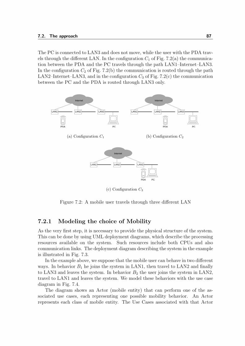
7.2. The approach 87
The PC is connected to LAN3 and does not move, while the user with the PDA trav-els through the different LAN. In the configuration C1 of Fig. 7.2(a) the communica-tion between the PDA and the PC travels through the path LAN1–Internet–LAN3.In the configuration C2 of Fig. 7.2(b) the communication is routed through the pathLAN2–Internet–LAN3, and in the configuration C3 of Fig. 7.2(c) the communicationbetween the PC and the PDA is routed through LAN3 only.
LAN1 LAN2 LAN3
PDA PC
Internet
(a) Configuration C1
LAN1 LAN2 LAN3
PCPDA
Internet
(b) Configuration C2
LAN1 LAN2 LAN3
PCPDA
Internet
(c) Configuration C3
Figure 7.2: A mobile user travels through three different LAN
7.2.1 Modeling the choice of Mobility
As the very first step, it is necessary to provide the physical structure of the system.This can be done by using UML deployment diagrams, which describe the processingresources available on the system. Such resources include both CPUs and alsocommunication links. The deployment diagram describing the system in the exampleis illustrated in Fig. 7.3.
In the example above, we suppose that the mobile user can behave in two differentways. In behavior B1 he joins the system in LAN1, then travel to LAN2 and finallyto LAN3 and leaves the system. In behavior B2 the user joins the system in LAN2,travel to LAN1 and leaves the system. We model these behaviors with the use casediagram in Fig. 7.4.
The diagram shows an Actor (mobile entity) that can perform one of the as-sociated use cases, each representing one possible mobility behavior. An Actorrepresents each class of mobile entity. The Use Cases associated with that Actor

88 7. An application to UML Mobility Modeling
Figure 7.3: Deployment diagram for the example
Figure 7.4: UML representation of different mobility possibilities
represent the different ways in which entities of the associated mobile entity classmay interact with the system. Note that this is perfectly consistent with the UMLsemantics of use case diagrams [74], as they are used to specify the behavior of anentity without specifying its internal structure.
7.2.2 Modeling Mobility Behaviors
The next step is to describe the order in which configurations are activated in eachbehavior. To do that, we associate an activity diagram to each use case; each activityof the activity diagram represents a configuration of the system. If the mobile usertriggers the configuration Cj immediately after the configuration Ci, then in theactivity diagram there will be a transition between the activity representing Ci andthe one representing Cj. Considering our example, the two behaviors B1 and B2 arerepresented as the activity diagrams of Fig. 7.5.
(a) Activity diagram associatedto B1
(b) Activity diagram asso-ciated to B2
Figure 7.5: Activity diagrams associated to the mobility behaviors
Note that in this way it is possible to represent non-determinism that is a be-

7.2. The approach 89
havior can have multiple successors. Fig. 7.6(a) illustrates an example where themobile entity starts by activating configuration A. Then it may proceed by acti-vating one of configuration B and C. After that, configuration D is activated. Itis important to observe that the activity diagrams associated to behaviors do notneed to be acyclic. Thus, it is also possible to model situations in which the usertriggers the same sequence of configurations for a number of times. Moreover, usingfork and join nodes of activity diagrams it is possible to represent the concurrentexecution of different configurations. This can be used to model situations in whichthe mobile entity generates copies of itself, each one traveling independently throughthe system. Fig. 7.6(b) shows an example where a mobile entity starts by enteringconfiguration A. Next, it splits in two copies, one executing configuration B and theother executing configuration C in parallel. This means that the two copies of themobile entity can move to different locations and perform different interactions withthe system. After that, the two copies synchronize and collapse into one instance,which proceeds by executing configuration D.
(a) (b)
Figure 7.6: Modeling nondeterministic mobility behavior 7.6(a) and mobile concur-rent execution of multiple agent instances 7.6(b)
7.2.3 Modeling Interactions between Components
The final step is describing the activities carried out in each configuration. To dothat, we use the hierarchical structure of the activity diagrams to associate theinteractions to each action state identified in the previous step. Namely, we expandeach action step representing a configuration into the activity graph describing thesequence of actions which are taken during the interaction between the mobile entityand the system. It is necessary to specify where the actions are executed. To do soit is possible to use “swimlanes”, which are a means for specifying responsibility foractions. The name of the swimlanes denotes the Deployment node instance on whichthe actions execute. As some graphical UML editors do not support swimlanes, it ispossible to tag each action with the PAhost tagged value, whose value is the nameof the node instance of the deployment diagram corresponding to the host wherethe action is executed. Fig. 7.7 shows the interactions performed while the systemwe are considering is in configuration C1 and C3 using the swimlane-based notation.
The interaction between the PDA and the PC is very simple. Basically, first the

90 7. An application to UML Mobility Modeling
(a) Interaction in configuration C1 (b) Interaction in configura-tion C3
Figure 7.7: UML description of the interactions
PDA computes which frames it needs. Then a suitable request is encoded and sentthrough the communication networks to the PC. The request is unmarshalled, andthe requested frames are encoded and packed into a reply message. This message issent back through the network to the PDA, which finally displays the frames. Notethat in Fig. 7.7 we omitted the description of the interaction in configuration C2,as this is basically the same as in C1, with the only difference that LAN2 is usedinstead of LAN1.
7.3 Summary of the UML Mobility Approach
The proposed mobility modeling approach can be summarized in the following steps:
1. Identify the processing resources (processors or networks) available in the sys-tem. Each resource is represented by a node instance in the UML deploymentdiagram.
2. Identify the classes of users of the system. Users represent workloads appliedto the system. Each class of users is represented as an Actor in the usecase diagram. Actor may represent either a fixed population of users (closedworkload) or an unlimited stream of users (open workload).
3. Identify the mobility behaviors. For each class of users it is necessary to iden-tify the different pattern of mobility they may exhibit. Each of such mobilitypatterns is represented by a use case associated to the Actor representing theclass of users.

7.4. A Simple Example 91
4. Provide a high level description of the mobility behaviors. An activity dia-gram is association to each of the use cases identified in the previous step.Such activity diagram represents the sequence of configuration changes whichhappens in the system while the mobile user moves.
5. Describe the interactions occurring in each system configuration. Each Ac-tion states defined in the previous step are expanded into a low-level activitydiagram describing the interactions between system entities. Each Action ofthe low-level diagram represents a service requested to a specific processingresource. Code mobility is represented by associated Activities in the low-level diagram to different hosts. Physical mobility is represented by a possiblydifferent interaction pattern associated to nodes of the high-level activity dia-gram.
Quantitative informations required by the simulator can be associated to UMLelements as described in Chapter 4. Each use case can be tagged with the probabilityof its occurrence, that is, the probability that the associated Actor (motile entity)will execute that use case (mobility behavior) upon arriving to the system. Actionstates of the high-level activity diagram associated to each use case can be annotatedwith the probability of occurrence, the number of times they are repeated andthe delay between repetitions. As each action state represents a configuration, theannotations allow the specify (nondeterministically) the pattern of mobility and howlong the system remains in each configuration. When the simulator “executes” aconfiguration, it basically executes all the activities of the low-level activity diagramembedded in the configurations.
A mobile code fragment moving from host H1 to host H2 is represented as follows.Let C1 be the configuration where the code executes in H1 and C2 the configurationwhere the code executed in H2. The low level activity diagram describing C1 andC2 will contain an action state (or a whole subdiagram) corresponding to the com-putation. Such action state or subdiagram will be tagged with the PAhost taggedvalue, which describes the location where the activity is executed. In C1 we setPAhost=H1, and in C2 we set PAhost=H2.
Physical mobility is modeled in a similar way. If a mobile device travels throughthe system, as in our example, probably it will interact with different other nodesfor communicating. Depending on the situation, it may even choose a differentcommunication pattern, and hence a different interaction style with other entities.Such interaction styles will be represented by (possibly different different) structuresof the low level activity diagrams.
7.4 A Simple Example
The case study illustrated in the previous sections has been simulated using theparameters reported on Table 7.1. A single user interacts with the system (closed

92 7. An application to UML Mobility Modeling
workload), and the probability p that the user triggers the behavior B1 (see Fig. 7.5)has been set to p = 0.3, while the probability that the user triggers the behavior B2
has been set to 1− p.
Parameter Value(Un)Marshalling Requests Constant 0.1s(Un)Marshalling Responses Exponential, mean=5.0sRequest Transmission Times Exponential, mean=1.0sResponse Transmission Times Exponential, mean=10.0sRequest Computation Exponential, mean=0.1sFrame Encoding Time Exponential, mean=20.0sDisplay time on the PDA Exponential, mean=20.0sPDA Speedup factor 0.2PC Speedup factor 10.0Processors Sched. Policies FIFO
Table 7.1: Simulation Parameters for the Mobile System Example
The simulation results are shown in Table 7.2. They are the steady-state meanvalues computed at 90% confidence level; for simplicity only the central value of theconfidence interval is shown.
Internet utilization 0.039LAN1 utilization 0.010LAN2 utilization 0.028LAN3 utilization 0.072PDA utilization 0.832PC utilization 0.015Behavior B1 response time 445sBehavior B2 response time 312s
Table 7.2: Simulation Results for the Mobile System Example.

IIIImplementation


8libcppsim: A process-oriented
simulation library
In this chapter we illustrate the design and implementation of libcppsim, a general-purpose, process-oriented simulation library written in C++. libcppsim providesthe user with a set of classes for implementing coroutines, simulation processes,the SQS data structure, and basic statistical functions for collecting and processingsimulation results. The basic simulation entity provided by the library is the simu-lation process : methods are provided for activating, stopping and rescheduling sim-ulation processes. The library provides simulation primitives which are commonlyimplemented in many process-oriented simulation languages or libraries, such as theSimula language [35].
The choice of the C++ programming language was motivated by the availabilityof efficient compilers and utility libraries (such as libraries for XML processing [62]),which greatly accelerated the simulator development. We implemented a minimal-istic set of simulation primitives in order to provide a simple and general frameworkon top of which more complex, high-level functionalities can be defined. Many ex-isting simulation packages are either special-purpose or not very efficient. For thatreason we decided to implement our own simulation toolkit which includes only theneeded functionalities. This simplified the debug of the simulation tool as we hadaccess to all the source code, and potential problems in the simulation library wouldreside in a restricted set of modules providing only simple functionalities.
8.1 Introduction and general concepts
The package structure of libcppsim is illustrated in Fig. 8.1; in the figure, UMLpackages denote sets of functionally related classes. There are two root packages:Coroutines and Variables. The Coroutines package provides two different implementa-tions of coroutines, which are used for implementing both simulation processes andthe Sequencing Set. The Variables package contains the basic definition of a “vari-able”, that is an entity which has a an internal state which can be updated withnew values; variables provides a method for computing a function of this internalstate. Using the abstraction of a “variable” it is possible to derive random number

96 8. libcppsim: A process-oriented simulation library
libcppsim
Processes
Coroutines Variables
StatisticsRandomNumberGenerators
SequencingSet
Figure 8.1: libcppsim package structure
generators and statistics classes. Random number generators are implemented asvariables returning a different value every time it is computed, thus producing astream of pseudo-random numbers. Statistics are special kind of variables whichare repeatedly updated with a sequence of observations of some quantity of inter-est computed by the simulation, and whose value is the requested statistics (mean,confidence interval, variance and others).
8.2 Coroutines
Coroutines are a programming construct which can be very helpful for implementingprocess-oriented simulation languages and libraries; Simula had coroutines as abuilt-in facility. Unfortunately, the C and C++ programming languages, which arewidely used and extremely efficient, do not provide coroutines natively.
Coroutines are blocks of code with associated state, which are activated accordingto the following rules:
• One coroutine at a time is active and is running; control is retained eitheruntil the coroutine terminates or until it explicitly resumes another coroutine.
• There exists a “main coroutine” which is the first coroutine being activated.The main coroutine gains control as soon as the program is executed.
• An active coroutine that gives up control by resuming another one retains itscurrent execution context. When the suspended coroutine is resumed, it willexecute from the point at which it last stopped.
Coroutines can be considered as a special kind of procedures, as defined in moststructured programming languages. For procedures there is a strict caller-calleeactivation order, that is, the caller procedures can transfer control to the calledone, and be reactivated only when the latter terminates. On the other hand controlcan flow arbitrarily for coroutines (see Fig. 8.2). Coroutines can be considered as

8.2. Coroutines 97
f() g() h() f() g() h()
Figure 8.2: Flow control for routines (left) and coroutines (right). Time advancesdownward. Thick lines represent which (co)routine is active at any given time.
a cooperative multithreading environment, with coroutines acting as lightweightthreads explicitly passing control each other.
Adding support for coroutines to the C++ programming language is not trivial.Each C++ function is associated to a data structure called activation record whichis stored in the run-time stack. The activation record contains informations aboutthe status of the routine, such as the value of the local variables. When a subroutinecall occurs, a new activation record for the called function is created and put on thetop of the stack. All the local variables, defined by the called routine, are storedon the newly created activation record. Similarly, when a routine terminates, itsactivation record is pushed from the stack. LIFO handling of the runtime stackdoes not work anymore with coroutines, because the currently active coroutine maynot be the one associated with the topmost activation record. This implies that theorder of activation of coroutines is not given by the LIFO stack handling.
This problem can be solved in different ways. The first approach is the “copy-stack implementation” described by Helsgaun [46]. The stack of the currently op-erating coroutine is kept in the C++ runtime stack. When a coroutine suspends,the runtime stack is copied in a buffer associated with the coroutine. The bufferis allocated in the dynamic heap, so it does not interfere with the normal stackoperation. A coroutine is resumed by copying the content of that buffer to C++’sruntime stack and setting the program counter to the saved execution location.While this approach is fairly portable, it makes the assumption that the run-timestack is implemented as a contiguous block of memory, as opposed to a linked listof frames.
A second approach is simpler and more portable, and consists of making useof the context handling facilities provided by most Unix SysV-like environments.The Operating System provides functions allowing user-level context switching be-tween different threads of control within a process. These functions are getcontext(),setcontext() and makecontext().
The getcontext() function is used to initialize a user-supplied data structure of

98 8. libcppsim: A process-oriented simulation library
type ucontext t with a copy of the current context. The ucontext t data structure isdefined as follows under the Linux OS [64] (in file /usr/include/asm/ucontext.h):
typedef struct ucontext{ unsigned long int uc_flags; struct ucontext *uc_link; /* Reference to the next context */ stack_t uc_stack; /* Where the stack for this context is located */ mcontext_t uc_mcontext; __sigset_t uc_sigmask; struct _fpstate __fpregs_mem;} ucontext_t;
The relevant fields of the structure are uc link which, if nonzero, points to the contextto be activated when this one terminates, and uc stack, which contains a pointer to adynamically allocated user memory area which holds the context. stack t is definedas follows:
typedef struct sigaltstack{ void *ss_sp; int ss_flags; size_t ss_size;} stack_t;
ss sp points to the stack.The makecontext() procedure modifies an ucontext t data structure; the user de-
fines a function which will be executed when the context is activated, and an optionalsuccessor context to be activated when the function terminates. The swapcontext()function saves the current context and activates a new one.
Both approaches have advantages and disadvantages. The “copy-stack” ap-proach requires a copy of the C++ runtime stack to be saved every time a coroutinepasses control, which may cause a considerable overhead. Moreover, the approachrequires that the run-time stack is internally represented as a contiguous block ofmemory (which however is the most common case in practice). The approach basedon the ucontext t data structure does not incur in this overhead, as the context eachcoroutine is allocated only once when the coroutine is activated. A coroutine switch(performed via the swapcontext() system call) just makes the CPU’s stack pointerto point to the stack of the coroutine to be resumed. This approach does not de-pend on the layout of the run-time stack, but does require the Operating Systemto support the makecontext and swapcontext system calls (old versions of Linux didnot implement them).
Unfortunately, the ucontext t based approach does not allow the coroutine con-text to grow past the dimension defined when the context is allocated. The user isrequired to set the maximum dimension of the context in advance; choosing a toosmall buffer results in weird runtime behaviors caused by stack corruption which

8.2. Coroutines 99
are typically very difficult to debug. The “copy-stack” approach does not havethis limitation. The libcppsim library implements both alternatives, and the usercan choose one at compile time. As a general rule, it is useful to use the “copy-stack” variant when developing the simulation program, in order to ensure that stackcorruption errors do not happen; then, when the program is checked and correct,production runs may be done with the more efficient context-based approach.
The coroutine class is defined as follows:
class coroutine{public: virtual ˜coroutine (); inline bool terminated( void ) const; void resume( void ); void call( void ); static size_t cStackSize;protected: coroutine( ); void detach( void ); virtual void main( void ) = 0; private: inline void enter( void ); coroutine *_caller; coroutine *_callee; static coroutine *_current_coroutine;};
Note that it is a virtual class, since the main() is pure virtual. Users can implementtheir own coroutines by inheriting a class from coroutine. The meaning of user-accessible methods (public and protected) is the following:
main() This method represents the body of the coroutine. When the coroutineobject is activated, the function main() is executed. The coroutine terminateswhen main() terminates.
bool terminated() Returns true if and only if the coroutine object represents aterminated coroutine, that is, a coroutine whose main() function finished.
call() This method is used for invoking a coroutine, setting the caller as the corou-tine to activate when this one terminates or performs a detach() operation.This method also sets the caller and callee pointers accordingly, so that whenthe caller terminates, control is automatically passed to the caller.
resume() Activates the coroutine from the main() function, if this is a newly createdcoroutine, or from the point it was last suspended. Note that this method doesnot set a caller-callee relationship between the coroutines. This means thatwhen the resumed coroutine terminates, control is not transferred to the onewho performed the resume() operation.
detach() Suspends the execution of the coroutine.

100 8. libcppsim: A process-oriented simulation library
coroutine+call()+resume()+terminated(): bool#detach()#main()-enter()
process-_id: int-_name: string+activate()+activateAfter(p:handle_p)+activateBefore(p:handle_p)+activateAt(t:double)+activateDelay(t:double)+reactivate()+reactivateAfter(p:handle_p)+reactivateBefore(p:handle_p)+reactivateAt(t:double)+reactivateDelay(t:double)+cancel()+idle(): bool+terminated(): bool+evTime(): double#passivate()#hold(t:double)#end_simulation()#inner_body()
absEvNotice#_time: double
sqs+insertAt(p:handle_p,t:double): absEvNotice*+insert(p:handle_p,q:handle_p): absEvNotice*+remove(ev:absEvNotice*)+clear()+first(): absEvNotice*+empty(): bool+size(): int
_ev
_proc
_sqs
shared-_sharedCount: int#getRef(): int#unGetRef(): int
handle+operator ->(): T*+operator (): T*+rep(): T*+isNull(): bool+setNull()
T
_obj
Figure 8.3: libcppsim process package class diagram
The enter() method is used to actually save save the context of the current coroutineand restore the context of the one control is passed to. Implementation details canbe found in Helsgaun [46].
8.3 Simulation processes
Once coroutines are available, it is very easy to define simulation processes on topof them. Fig. 8.3 shows the class hierarchy related to simulation process implemen-tation.
A simulation process is represented by the process class, and it inherits fromcoroutine. Simulation processes implement their functionalities in term of the basicactivation primitives provided by the coroutine class.
Each simulation process has a unique identifier and a user-supplied (not necessar-ily unique) name. The process class implements methods providing all the schedulingprimitives described in Section 3.4. The actions performed by the simulation processshould be specified by redefining the pure virtual method inner body().
One feature which was missing from the initial implementation of the processclass was a mechanism for automatic garbage collection. This is a feature whichis not present in the C/C++ languages, but is extremely valuable when writingsimulation programs. The reason is that when many simulation processes are dy-namically created, it is often desirable to have them automatically destroyed whenthey terminate and are not reachable from any live pointer.
It turns out that the implementation of a complete garbage collector was not

8.4. Sequencing Set implementations 101
really necessary. Instead, we chose to implement a simpler mechanism based onsmart pointers. A smart pointer is represented by the templated class handle〉T〈,which represents a reference to an object of type T which can be shared amongmultiple owners. When the last handle containing a reference to some object goesout of scope and is deallocated, then the referenced object is automatically destroyedand its memory reclaimed. The implementation of the handle class is based onthe reference-count idea described in [94]. Basically, the handle class redefines theconstructor, destructor and assignment operator in order to maintain a count ofthe number of active references to the shared object. When this counter goes tozero, the object is destroyed. Our implementation is however slightly different inthat the reference count is kept inside the shared object. This requires that, inorder to be put inside an handle〈T〉, the type T must be derived from the sharedclass, which contains just a counter and operators to increment and decrement it.This approach has the disadvantage that not every data type can be used inside anhandle (e.g., it is impossible to have an handle〈double〉), but it has the advantagethat the reference count is preserved even when a handle〈T〉 is dereferenced as anobject of type “pointer to T” and then back to a different hanlde〈T〉. That is, in thefollowing fragment of code, with our implementation of handles, the reference countis preserved correctly:
int foo( void ){ handle<process> p = get_some_process( ); process* r = p.rep( ); // Dereference p handle<process> q( r ); // OK. reference count preserved}
Situations like that happen in the implementation of some methods of the processand sqs classes, and are unavoidable. Note that sharing the same object betweenhandles and ordinary C++ pointers may cause problems, as handles may cause theshared object to be destroyed, making pointers invalid.
Simulation processes may be associated with an event notice, represented by aninstance of a class derived from absEvNotice. The event notice basically containsthe simulation time the process must be activated, and its position in the SQS. Thelatter is clearly dependent upon how the SQS data structure is implemented. Hence,every SQS implementation defines its own specialized version of event notice.
8.4 Sequencing Set implementations
The Sequencing Set (SQS), as described in Section 3.4, is a data structure containingthe set of simulation processes to activate sorted by nondecreasing timestamp order.Thus, it is basically a priority queue, where the priority is given by the process(re)activation time. Each simulation process contained in the SQS is associatedwith an event notice. We keep event notices as separate entities (derived from the

102 8. libcppsim: A process-oriented simulation library
sqsabsEvNotice
dllEvNoticeprioEvNotice sqsDllsqsPrio1_sqs
0..*1_sqs
0..*
Figure 8.4: libcppsim Sequencing Set class diagram
absEvNotice class) in order to be able to provide different implementations of thesequencing set data structure, each one needing particular informations in its eventnotices. We provide two different implementations of the SQS data structure (seeFig, 8.4).
The first implementation is contained in class sqsDll, and is based on a simpledoubly linked list. This data structure is very simple, but inserting an element inthe list requires linear time on average. A more efficient implementation, based onbalanced search trees, is given in class sqsPrio. The expected insertion time in thiscase is proportional to the logarithm of the SQS size.
8.5 Random variate generations
Each simulation engine should provide an efficient and statistically robust mech-anism for producing streams of pseudo-random numbers with given distribution.libcppsim defines an abstract templated class rng〈T〉 representing a pseudo-randomnumber generator producing a stream of numbers of type T . Thus, it is possibleto generate streams of random integers, real or boolean values, by setting T tothe appropriate datatype in a subclass. The rng〈T〉 class hierarchy is depicted inFig. 8.5.
It turns out that the basic ingredient for generating stream of pseudo-randomnumbers is a good uniform generator RN(0, 1) over the interval [0..1]. We chose toimplement algorithm MRG32k3a from L’Ecuyer [61], which is known to have longperiod and very good statistical properties, other than being very efficient. In thepseudocode used below, rngUniform01() denotes the implementation of this ran-dom number generator.
The following random variate generators are currently implemented. The imple-mentations are taken from [16, Ch. 5].
Uniform distribution: U(a, b), a < b
It is implemented by class rngUniform.

8.5. Random variate generations 103
rngBernoulli#_p: double
T:boolrngNormal
#_mu: double#_sigmasq: double
T:doublerngDiscEmprical
#_p: vector<double>
T:int
rngT
rngGam#_a: double#_b: double
T:double
rngErl#_m: double#_k: int
T:double
rngWeib#_a: double#_b: double
T:double
rngExp#_mean: double
T:double
rngUniform#_a: double#_b: double
T:double
rngDiscUniform#_a: int#_b: int
T:int
rngConst#_mean: double
T:double
rngLTNormal#_mu: double#_sigmasq: double#_l: double
T:doublerngRTNormal
#_mu: double#_sigmasq: double#_r: double
T:doublerngLRTNormal
#_mu: double#_sigmasq: double#_l: double#_r: double
T:double
Figure 8.5: libcppsim Random Number Generators class diagram
Density:
f(x) =
1
b− aa < x < b
0 otherwise
Distribution function:
F (x) =
0 x ≤ ax− a
b− aa < x < b
1 x ≥ b
Generator:rng<double> U1 = rngUniform01( );return U1.value( )*(_b - _a) + _a;
Exponential distribution: EXP(a), a > 0
It is implemented by class rngExp.The parameter a > 0 is the mean of the distribution. The rate parameter is a−1.
Density:
f(x) =
{a−1 exp
(−x
a
)x > 0
0 otherwise
Distribution function:
F (x) =
{1− exp
(−x
a
)x > 0
0 otherwise
Generator:

104 8. libcppsim: A process-oriented simulation library
rng<double> U1 = rngUniform01( );return (double)(- _mean*log( 1.0 - U1.value( ) ) );
Weibull distribution: WEIB(a, b), a, b > 0
It is implemented by class rngWeib.Density:
f(x) =
ba−bxb−1 exp
[−
(x
a
)b]
x > 0
0 otherwise
Distribution function:
F (x) =
1− exp
[−
(x
a
)b]
x > 0
0 otherwise
Generator:
rng<double> U1 = rngUniform01( );// pow( a, b ) returns a raised to the b powerreturn _a*pow( -log( 1.0 - U1.value() ), 1.0/_b );
Gamma distribution: GAM(a, b), a, b > 0
It is implemented by class rngGam.Density:
f(x) =
(x/a)b−1
aΓ(b)exp
(−x
a
)x > 0
0 otherwise
where Γ(b) is the gamma function:
Γ(b) =
∫ ∞
0
ub−1e−udu
The distribution function has no simple closed form.Generator:

8.5. Random variate generations 105
rng<double> U1 = rngUniform01();rng<double> U2 = rngUniform01();// M_E = e = 2.71828...if ( b < 1.0 ) { const double beta = (M_E+b)/M_E; while( 1 ) { double U = U1.value( ); double W = beta*U; double V = U2.value( ); if ( W < 1.0 ) { double Y = pow( W, 1.0/b ); if ( V <= exp( -Y ) ) return a*Y; } else { double Y = -log( (beta-W)/b ); if ( V <= pow(Y, b-1.0) ) return a*Y; } }} else if ( b < 5.0 ) { while( 1 ) { double U_1 = U1.value( ); double U_2 = U2.value( ); double V_1 = -log( U_1 ); double V_2 = -log( U_2 ); if ( V_2 > ( b-1.0 )*( V_1-log( V_1 )-1.0 ) ) return a*V_1; }} else { double alpha = 1.0/sqrt( 2.0*b - 1.0 ); double beta = b - log(4.0); double gamma = b + 1.0/alpha; double delta = 1.0 + log( 4.5 ); while( 1 ) { double U_1 = U1.value( ); double U_2 = U2.value( ); double V = alpha*log( U_1/(1.0-U_1) ); double Y = b*exp( V ); double Z = U_1 * U_1 * U_2; double W = beta + gamma*V - Y; if ( W+delta-4.5*Z >= 0 ) return a*Y; else if ( W >= log( Z ) ) return a*Y; }}
k-Erlang distribution: ERL(m, k), m > 0, k positive integer
It is implemented by class rngErl.Density: the same as that of GAM(m/k, k).Distribution function: No closed form for the general case.Generator:

106 8. libcppsim: A process-oriented simulation library
if ( k < 10 ) { rng<double> U1 = rngUniform01(); double prod = 1.0; for ( int i=0; i<k; i++ ) prod *= ( 1.0 - U1.value() ); return -( m/(double)k )*log( prod );} else { rng<double> U2 = rngGam( m/(double)k, k ); return U2.value();}
Normal distribution: N(µ, σ2), σ > 0
It is implemented by class rngNormal.µ is the mean and σ2 is the variance of the distribution. Density:
f(x) =1
σ√
2πexp
[−(x− µ)2
2σ2
]Distribution function: No closed form expression.Generator:
rng<double> U1 = rngUniform01();rng<double> U2 = rngUniform01();// M_PI = pi = 3.1415...double R = sqrt( -2.0*log( U1.value( ) ) );double T = 2.0*M_PI*U2.value( );val[0] = mu + sigma*( R*cos( T ) );val[1] = mu + sigma*( R*sin( T ) );return val[0] and val[1];
Truncated Normal distributions: NL(µ, σ2, l), NR(µ, σ2, r), NLR(µ, σ2, l, r), σ >0
These distributions are similar to the Normal distribution, except that the range ofvalues they can assume is constrained to the left, to the right or both.
µ is the mean and σ2 is the variance of the distribution. l is the the left truncationpoint, and r is the right truncation point.
Let
g(x) =1
σ√
2πexp
[−(x− µ)2
2σ2
]−∞ < x <∞
The density function fL for the Left Truncated Normal distribution NL(µ, σ2, l)is defined as:
fL(x) =
0 if x ≥ l
g(x)∫ +∞l
g(x)dxotherwise
Generator:

8.5. Random variate generations 107
rng<double> U1 = rngNormal(mu, sigmasq);double result;do { result = U1.value();} while ( result < l );return result;
The density function fR for the Right Truncated Normal distribution NR(µ, σ2, r)is defined as:
fR(x) =
g(x)∫ r
−∞ g(x)dxif x ≤ r
0 otherwise
Finally, the density function fLR of the Left and Right Truncated Normal dis-tribution NLR(µ, σ2, l, r) is defined as:
fLR(x) =
g(x)∫ r
lg(x)dx
if l ≤ x ≤ r
0 otherwise
Generator functions are very similar to the one for the Left Truncated Normaldistribution.
Constant distribution: C(µ)
It is implemented by class rngConst.This distribution always returns the constant value µ, and is trivially imple-
mented.
Bernoulli distribution: BER(p), 0 < p < 1
Probability mass function:
X =
{1 with probability p
0 with probability 1− p
Generator:
rng<double> U1 = rngUniform01();return ( U1.value( ) <= p );
Empirical Distribution
This distribution is implemented by class rngDiscEmpirical. Let us consider a setof probabilities p0, p1, . . . pn−1 such that for each i = 0, . . . n − 1, 0 ≤ pi ≤ 1, and

108 8. libcppsim: A process-oriented simulation library
∑n−1i=0 pi = 1. The empirical distribution returns one of the integers [0, 1, . . . n − 1]
with probabilities [p0, p1, . . . pn−1] respectively.
P (X = i) =
{pi if i = 0, 1, . . . n− 1
0 otherwise
The generator can then be expressed as:
rng<double> U1 = rngUniform01();const double tmp = U1.value( );double sum = 0.0;int i;// p is the vector of probabilitiesfor ( i=0; i<(int)p.size( )-1; i++ ) { sum += p[i]; if ( tmp < sum ) break;}return (int)i;
Discrete Uniform DISCU(a, b), a < b integers
This generator is implemented by class rngDiscUniform. The probability mass func-tion is:
P (X = i) =
1
b− a + 1if i ∈ [a, a + 1, . . . b]
0 otherwise
8.6 Output Data Analysis
Simulation results are typically a sequence of observations of quantities of interest.For example, let us consider a road traffic simulation. Suppose that the modeler isinterested in computing the mean number of cars crossing a bridge each day. Thesimulation produces a sequence of observations X1, X2, . . . Xn corresponding to thenumber of cars crossing the bridge on day 1, 2, . . . n. Unfortunately, the estimatorX = 1
n
∑Xi is in general a biased estimator of the mean X. The reason is that the
observations X1, X2, . . . Xn are in general autocorrelated, and thus not statisticallyindependent. In addition to the autocorrelation problem, the initial conditions ofthe simulation must be accurately chosen, since they may effect all the computedobservations.
libcppsim implements a set of classes dealing with collection of statistics. Fig-ure 8.6 shows the relevant portion of the class diagram.
All types of statistical variables inherit from the var〈Tin, Tout〉 abstract baseclass. Class var represents “variables” which can be updated many times by feedingvariables of type Tin, and compute some function from the input data as a result oftype Tout. Each variable has a (not necessarily unique) name, and supports two purevirtual methods: update() and reset(). These are used to insert a new value and reset

8.6. Output Data Analysis 109
var#_name: string#_numUpdates: int#_numResets: int+update(v:T_in)+reset()+value(): T_out+report()
T_inT_out
confInt+_lBound: double+_uBound: double+_confl: double
statistic#_confl+setConfl(c:double): double+getConfl(): double
T_in:doubleT_out:confInt
mean repmean welch
histogramaccum bmeans
trremoval#_ob: vector<double>
T_in:doubleT_out:vector<double>
trremoval_frac#_frac: double
trremoval_const#_l: int
rng
T_in:doubleT_out
Figure 8.6: libcppsim statistics class diagram
the variable to a known state. The result can be computed by invoking the value()method. Variables are not stateless; thus, it is possible that successive repeatedinvocations of the value() method return different results. This is particularly useful,as a random stream can be represented as a special kind of variable which can beupdated with the seed of the pseudo-random number generator, and whose value()method returns the next pseudo-random number from the stream, at the same timeupdating the seeds. Class var defines also a pure abstract report() method whichcan be used to display a report about the content of the class.
The statistics class represents a base class for a number of predefined statisticfunctions. In addition to the methods and attributes defined in its parent class var,statistics contains an attribute representing the confidence level of the computedresult.
The trremoval class is used to model algorithms dealing with the removal of theinitialization bias from a sequence of observations. Suppose that the simulation runproduces the sequence of observations Y1, Y2, . . . Yn for some parameter of interest.In general using the whole sequence to compute the statistics is dangerous as thereis a bias associated to artificial or arbitrary initial conditions. One method toovercome this limitation is to divide the sequence of observations into two phases:first an initialization phase including observations Y1, Y2, . . . Yd, followed by a data-collection phase Yd+1, Yd+2 . . . Yn. The parameter d, 0 < d � n is called truncationpoint. Classes inheriting from trremoval are used to identify the truncation point daccording to some specific algorithm.

110 8. libcppsim: A process-oriented simulation library
mean
This class is used to compute a confidence interval for the mean of a sequence ofstatistically uncorrelated observations Y1, Y2, . . . Yn. The point estimator Y of themean Y , is computed as [17]:
Y =1
n
n∑i=1
Yi (8.1)
The approximate 100(1− α)% confidence interval for Y is computed as
Y − tα/2,fσ(Y ) ≤ E(Y ) ≤ Y + tα/2,fσ(Y ) (8.2)
where tα/2,f is the 100(1 − α/2)% percentage point of a t-distribution with fdegrees of freedom; that is, tα/2,f is defined by P (t ≥ tα/2,f = α/2. Also,
σ2(Y ) =1
n(n− 1)
n∑i=1
(Y − Yi)2
accum
This class is used to compute a time-weighted sum of observations Y1, Y2, . . . Yn,n > 1 with timestamps respectively t1, t2, . . . tn. The result is computed as
A =n−1∑i=1
Yi(ti+1 − ti)
repmean
One method of computing the mean of observations Y1, Y2, . . . Yn is called the methodof independent replications. The simulation is repeated a total of R times, each runusing a different random number stream and independently chosen initial condi-tions. Let Yri be the ith observation within replication r, for i = 1, 2, . . . nr andr = 1, 2, . . . R. For fixed replication r, Yr1, Yr2, . . . Yrnr is a possibly autocorrelatedsequence of observations. However, for different replications r 6= s, Yri and Ysj arestatistically independent. We compute the sample mean Yr within each replicationr by
Yr =1
nr
nr∑i=1
Yri r = 1, 2, . . . R
The R sample means Y1, Y2, . . . Yn are statistically independent and identicallydistributed. Then, a confidence interval for the mean Y can be computed by Eq. 8.2.The method reset() is used in class repmean to start a new replication.
Note that this class depends on the trremoval class. This is because a strategyfor removing the initialization bias must be provided when creating an object of

8.6. Output Data Analysis 111
type repmean. By default a simple strategy consisting of deleting the first 20% ofeach replication is employed.
bmeans
The method of batch means divides the output data from one replication (afterdeleting an appropriate amount of the initial observations) into a number of batches,and then treating the means of these batches as if they were independent. Let usconsider the sequence Yd+1, Yd+2, . . . Yn after deleting the first d observations. Weform k batches of size m = (n− d)/k and compute the batch means as:
Yj =
jn∑i=(j−1)n+1
Yi+d (8.3)
for j = 1, 2, . . . k (we assume k divides n−d evenly). The variance of the samplemean is estimated by
S2
k=
1
k
k∑j=1
(Yj − Y )2
k − 1=
∑kj=1 Y 2
j − kY 2
k(k − 1)(8.4)
where Y is the overall sample mean of the data after deletion. The batch meansY1, Y2, . . . Yk, even if not independent, are approximately independent for large batchsizes. The reader is referred to [16, 17, 60] for guidelines on setting appropriate valuesfor the batch size k.
Within the class bmeans the user can call the method reset() is used to start anew replication.
Note that this class depends on the trremoval class. This is because a strategyfor removing the initialization bias must be provided when creating an object oftype bmeans. By default a simple strategy consisting of deleting the first 20% of theobservations is employed.
welch
This class implements the graphical procedure of Welch [99] for identifying the lengthof the initial transient period. Let us consider R independent replications, of lengthn each: replication r produces the observations Yr1, Yr2, . . . Yrn, where r = 1, 2, . . . R.First, we compute the average across the repetitions:
Y i =1
R
R∑j=1
Yji i = 1, 2, . . . n (8.5)

112 8. libcppsim: A process-oriented simulation library
Ensemble average are smoothed by plotting a moving average, considering timewindow of length w:
Yj(w) =
1
2w + 1
w∑m=−w
Yj+m w + 1 ≤ j ≤ n− w
1
2j − 1
j−1∑m=−j+1
Yj+m 1 ≤ j ≤ w
(8.6)
The graph of Yj(w) is less variable as j increases. The truncation point is thevalue of j at which the plot definitely stabilizes.
The user should invoke the update() method of this class in order to add anew observation value for the current replication. The method reset() is used toterminate the current replication, and start a new one. The plot is produced bycalling the method report(); it produces a file named rep.<histogram_name> whichcan be processed by the gnuplot tool [42].
histogram
This class computes an histogram profile from the inserted values Y1, Y2, . . . Yn. Theuser supplies an expected lower bound and upper bound for the observed values.Also, the user specifies the number of cells (bins) in which the histogram will bedivided. Instances of the class histogram do not compute anything using the value()method. Users are expected to call the report() method to print the informationsconcerning an histogram. A sample printout is presented in Fig. 8.7.
The problem of initialization bias
One of the most difficult problems in steady-state simulation output analysis is theremovel of the initialization bias [16]. The problem can be stated as follows. Let Ithe set of initial conditions for the simulation model and assume that as n → ∞,P (Xn ≤ x|I) → P (X ≤ x), where {Xi} is the stochastic process correspondingto the sequence of observed values from the simulation, and X is the steady-staterandom variable. The steady-state mean of the process {Xi} is µ = limn→∞E(Xn|I).The problem with the use of the estimator Xn = 1
n
∑ni=1 Xi for a finite n is that
E(Xn|I) 6= µ, and thus X(Xn|I) 6= µ.As an example, consider the computation of the average waiting time on a simple
M/M/1 queue shown in Fig. 8.8. This is a system made of a single server with anunlimited buffer (queue) of waiting customers served in FIFO order. The interarrivaltime of customers is modeled by an exponentially distributed random variable withrate τ = 0.09 and service rate ω = 0.1. Fig. 8.8 shows the mean waiting timecomputed after averaging 50 independent replications of the simulation experiment,and after the plot has been smoothed with Welch’ approach, with window sizew = 500. We can see that the first d observations of the mean waiting time, with

8.6. Output Data Analysis 113
Name / Obs / N / min / max / mean / std.devNormal / 50000 / 22 / -4.02 / 4.09 / -0.00 / 1.00
bin/ low.bound/ bin% / cum% / Histogram /count0/ -INFTY/ 0.00/ 0.00/ /01/ -5.00/ 0.00/ 0.00/ /02/ -4.50/ 0.00/ 0.00/. /13/ -4.00/ 0.01/ 0.01/. /44/ -3.50/ 0.07/ 0.08/. /355/ -3.00/ 0.52/ 0.60/. /2586/ -2.50/ 1.74/ 2.34/*** /8707/ -2.00/ 4.47/ 6.81/******** /22368/ -1.50/ 9.19/ 16.00/**************** /45969/ -1.00/ 15.05/ 31.05/*************************** /752410/ -0.50/ 19.23/ 50.27/***********************************/961311/ 0.00/ 18.84/ 69.12/********************************** /942112/ 0.50/ 15.13/ 84.24/*************************** /756413/ 1.00/ 9.17/ 93.42/**************** /458614/ 1.50/ 4.31/ 97.73/******* /215515/ 2.00/ 1.66/ 99.39/*** /83016/ 2.50/ 0.48/ 99.87/. /24117/ 3.00/ 0.11/ 99.98/. /5518/ 3.50/ 0.02/100.00/. /919/ 4.00/ 0.00/100.00/. /2All remaining bins are 0
Figure 8.7: Sample histogram printout
d ≈ 1000, are consistently lower than the real waiting time. If those values areincluded in the computation of the mean waiting time, the result will be highlybiased and the confidence interval will be larger.
Currently, there is no automatic method for detecting the length of the initializa-tion bias which can be proven correct in every situation. Different approaches havebeen proposed in the literature [101], although their general effectiveness is dubious,and strongly depends on the specific simulation model to which they are applied.For that reason, simulation packages usually implement one of the following simplestrategies:
• Removing a prefix consisting of a fixed fraction (eg, 20%) from the sequenceof observations;
• Performing a very long simulation run such that the effect of the initial tran-sient period can be neglected.

114 8. libcppsim: A process-oriented simulation library
0
20
40
60
80
100
120
0 1000 2000 3000 4000 5000 6000 7000 8000
Wai
ting
Tim
e
Observation #
Waiting TimeSimulation Average
Figure 8.8: Average waiting time for the first 8000 customers of an M/M/1 queuefrom 50 independent replications. Moving averages with window size w = 500 areplotted
trremoval const
This class represents a very simple strategy for removing the initialization bias.It basically discards the first d observations from the sequence Y1, Y2, . . . Yn,where d is specified by the user. The value() method returns the vector of valuesYd+1, Yd+2 . . . Yn, if more than d values have been inserted using the update()method.
trremoval frac
This class implements the initialization bias removal strategy consisting in removinga prefix of the sequence of observations Y1, Y2, . . . Yn of length bn×fc, with 0 ≤ f ≤1, and b·c denoting rounding to the nearest lower integer.

9UML-Ψ Tool Description
In this chapter we describe the UML-Ψ prototype tool which has been built in orderto show how the general approach described in Part II can be applied in practice.
9.1 Introduction
The UML-Ψ tool parses a software model annotated according to the UML profiledescribed in Chapter 5. The model has to be exported in XMI format [76], which isan XML-based representation of the UML model. Unfortunately, the XMI notationdescribed in the standard can be implemented in different (and incompatible) waysby CASE tool vendors. This constitutes an obstacle to large-scale adoption of XMIas platform-neutral representation of UML models. UML-Ψ understands the XMIdialect used by the freely available ArgoUML modeling tool [2], and its commercialcounterpart Poseidon [80]. ArgoUML version 0.12 and Poseidon version 1.4 havebeen tested. Note that UML-Ψ is known not to work with Poseidon version 1.6, asthe XMI format it employs is different and incompatible with previous versions.
UML-Ψ builds an internal representation of the UML model; only the portionsof the model which are relevant for the performance evaluation model constructionare considered. At this point the internal UML model representation is used tobuild the simulation performance model. The simulation model is based on the onepresented in Fig, 4.4, p. 46.
Once the performance model is set up, UML-Ψ starts the simulation by activatingthe simulation processes representing the workloads and the resources. The workloadprocesses create the requests arriving to the system, which in turn will activate thecorresponding activity diagrams. The simulation stops when one of the followingconditions becomes true first:
• The simulation time reached a user-defined maximum value;
• All the performance measures computed during the simulation convergedwithin the given confidence interval width.
In Fig. 9.1 we depict the high-level structure of the UML-Ψ model processingframework. The UML model is created using a CASE tool. At the moment, UML-Ψ has been tested with the models generated by ArgoUML [2] version 0.12 and its

116 9. UML-Ψ Tool Description
UML CASETool
XMIRepresentation
XMI Parser
Process-OrientedSimulation Model
ModelExecutor Parameters
Internal Rep.of the UML Model
SimulationModel Builder
Figure 9.1: The UML-Ψ model processing framework
commercial counterpart Poseidon [80], version 1.4. The annotated UML model hasto be exported in XMI format. Due to different implementations of the XMI formatby different tool vendors, it is at the moment not possible to use UML-Ψ with otherCASE tools. In fact the XMI specification [76] did not attempt to create an officialmetamodel for UML.
Once the XMI representation of the UML software system has been created, theUML-Ψ tool parses the XML document and builds an internal simplified represen-tation of the relevant portions of the UML SA.
From this internal representation, a simulation model is derived. The model isexecuted by considering both the parameters specified by the user (tagged valuesassociated to UML elements), and also by including a configuration file. This con-figuration file can be an arbitrary fragment of Perl code. After this code has beenparsed, the Perl interpreter environment (modified by every declaration containedin the configuration file) is used to parse the tagged values. Hence, the configura-tion file may be used to define Perl variables which are used inside tagged values.The user may then explore different performance behaviors for different values ofthese variables by simply changing the configuration file, without affecting the UMLmodel.
Finally, the simulation performance model is executed. The computed results areinserted into the XMI document as tagged values associated with the UML elementsthey refer. It is possible to use the CASE tool to reopen the UML model in order

9.2. UML-Ψ class diagram 117
simObjectumlObject
umlModel
umlActor
umlUseCase
umlNode
*
*
*
umlActionBase
umlCompositeAction
umlSimpleAction
umlPseudoState
umlFinalState
_content
umlTransition
_outTransitions*
simActionBase
simTransition
simModel
simResource
_outTransitions*
_resources*
process
simWorkload
umlStereotype
umlTaggedValue
0..1
*
_activity
_workloads
Figure 9.2: UML-Ψ class diagram, main part
to see the results. The performance modeling cycle may be repeated many times,until the performance goals have been satisfied.
9.2 UML-Ψ class diagram
A portion of the class diagram for the UML-Ψ tool is given in Fig. 9.2. The diagramshows on the left part the classes used for representing the UML model which isreconstructed from the XMI representation provided as input. On the right part,portion of the classes which are used to build the simulation model can be seen. Weobserve the almost direct correspondence between UML elements and simulationprocesses. There is a one-to-one mapping between a workload process and thecorresponding UML actor; the simulation model is as a whole associated to theUML model. Finally, each resource (active or passive) corresponds to a node inthe depoloyment diagram. Simulation actions are associated to action states inActivity diagrams, and transitions between actions are the simulation counterpartof transitions between action states.
9.3 UML model representation
The class hierarchy concerning the UML model has its root in the umlObject class.This class contains the common attributes and basic operations of all UML modelelements. Each UML object can be stereotyped with at most one stereotype, andmay have an arbitrary number of tagged values associated with it. Stereotypes andtagged values are represented as objects of class umlStereotype and umlTaggedValue

118 9. UML-Ψ Tool Description
simCompositeAction
simCallAction
simForkAction
simJoinAction
simResActionBasesimAcquireAction
simReleaseAction
simActionBase1..*
simPassiveResource *
1
1
*
simSimpleAction
simActiveResource0..1
Figure 9.3: Class diagram for UML-Ψ simulation actions
respectively. A UML model is represented by class umlModel, which contains objectsof class umlActor, umlUseCase and umlNode. They represent actors, use cases anddeployment diagram nodes respectively. A use case is associated with a compositeaction which describes its behavior.
The common features of UML actions are represented in class umlActionBase.This abstract class contains a reference to a list of outgoing transitions(umlTransition). A transition, in turn, is associated to a source and a target action.The different kind of actions in UML models are represented by classes inheritingfrom umlActionBase. These are: composite actions (umlCompositeAction), simpleactions (umlSimpleAction), pseudo states (umlPseudoState, which correspond to forkand join nodes, for example) and the final state (umlFinalState).
9.4 Simulation model representation
The structure of the simulation model, whose top portion is reported on the rightside of Fig. 9.2, is similar to that just seen for the UML model representation.The root class of the hierarchy is simObject (derived from the process class of thelibcppsim library). Simulation actions, workloads and resources are represented byclass simActionBase, simWorkload and simResource respectively, all inheriting fromthe base simObject class.
The class hierarchy representing simulation actions is shown in Fig. 9.3. Theclass hierarchy follows a pattern similar to that of the corresponding UML modelrepresentation. The root class is simActionBase. Its dynamic behavior (that is, thebody of the inner body() method inherited from the process class) is not specified;this allows subclasses to implement specific behaviors, according to their type. Sub-classes are defined to implement atomic actions (simSimpleAction), composite actions(simCompositeAction), fork and join nodes (simForkAction and simJoinAction respec-tively), actions dealing with passive resources (simResActionBase), and the specialcall action (simCallAction). A call action is needed to overcome a limitation of Ar-

9.4. Simulation model representation 119
simWorkload
simOpenWorkload simClosedWorkload
Figure 9.4: Class diagram for UML-Ψ simulation workloads
simResource
simActiveResource simPassiveResource
simPRhost_FIFO
simPRhost_LIFO
simPRhost_PS
Figure 9.5: Class diagram for UML-Ψ simulation resources
goUML and Poseidon, which at the moment do not provide functionalities to definecomposite actions, even if they are defined in the UML standard. As a workaround,a composite action is modeled as follows. The user must specify a use case associatedwith the content of the composite action. This is necessary as ArgoUML/Poseidondo not allow users to create an activity diagram without it being used to specifya class or use case behavior. At this point, a simple (atomic) action is used wherethe composite action would have been put. This atomic action is stereotyped as�PAcompositeStep�. A tagged value labeled ActivateUC must contain the nameof the use case to activate when the action is to be executed.
The class diagram representing simulation workloads, depicted in Fig. 9.4, is verysimple; a simWorkload virtual base class is used to represent a generic workload,whereas specialized simOpenWorkload and simClosedWorkload classes are used tomodel open and closed simulation workload processes respectively.
Finally, Fig. 9.5 depicts the class diagram of UML-Ψ processes representing activeand passive resources. The simResource virtual base class is the root of the resourceprocesses hierarchy. Resources are specialized in active resources, or processors(simActiveResource) and passive resources (simPassiveResource). Active resourcesare specialized again depending on their scheduling policy. Hence, we define aclass representing a simulation process of a processor with FIFO scheduling policy(simPRHost FIFO), one for the LIFO scheduling policy (simPRHost LIFO) and onefor the Processor Sharing (PS) scheduling policy (simPRHost PS). Adding morescheduling policies to the simulation engine requires the user to derive a suitableclass from simActiveResource.

120 9. UML-Ψ Tool Description

10The NICE Case Study
10.1 Introduction
In this chapter we apply the performance evaluation approach and the UML-Ψ toolpreviously introduced to the NICE case study from [7]. We show how performanceanalysis can be performed on early UML models in order to verify if the SA satisfiesits performance requirements set by the system commissioner. This case study is inpart motivated by the fact that it proved to be difficult to handle using analyticalsoftware performance evaluation techniques (in particular, using Process Algebras)due to the state-space explosion problem [24, 32]. The simulation-based approachwe apply is of course immune to such problem.
Naval Integrated Communication Environment (NICE) is a project developedby Marconi Selenia. It provides communications for voice, data and video in anaval communication environment. It also provides remote control and monitoringin order to detect equipment failures in the transmission/reception radio chain. Itmanages the system elements and data distribution services, enables system aidedmessage preparation, processing, storage, retrieval distribution and purging, and itimplements radio frequency transmission and reception, variable power control andmodulation and communications security techniques. The system involves severaloperational consoles that manage the heterogeneous system equipment including theATM based Communication Transfer System (CTS) through blind Proxy computers.
On a gross grain the Software Architecture is composed of the NICE Man-agement subsystem (NICE MS), CTS and EQUIP subsystems, as highlighted inFig. 10.1. The WORKSTATION subsystem represents the management entity,while the PROXY AGENT and the CTS PROXY AGENT subsystems representthe interface to control the EQUIP and the CTS subsystems, respectively.
Actually, the real configuration of the software system will be composed by oneinstance of WORKSTATION subsystem, two instances of CTS PROXY AGENTsubsystem, ten instances of PROXY AGENT subsystem and at least twenty EQUIPsubsystem instances. In general, a PROXY AGENT instance manages at least twoEQUIP instances.
The more critical component is the NICE MS subsystem. It controls both inter-nal and external communications and it satisfies the following class of requirements:

122 10. The NICE Case Study
C1
WORKSTATION
CTS PROXY AGENT
NICE-MS
EQUIP
CTS
C2
- PROXY AGENT
Figure 10.1: NICE static software description
fault and damage management, system configuration, security management, traf-fic accounting and performance management. All these class of requirements mustsatisfy some particular performance constraints. For the sake of the presentation,in this work we focus on two scenarios representing two crucial activities of theNICE system: Equip Configuration and Recovery activities. The two scenarios aredescribed in Fig. 10.2. The estimated execution times of the various actions areexponentially distributed random variables; the mean values were provided by thesystem developers and are reported in Fig. 10.3.
10.2 Equip Configuration Scenario
The configuration scenario is activated by an operator when new parameter setting ofone or more equipments is required. The system configuration activity consists in aset of actions having the aim the reconfiguration of any equipment (see Fig. 10.2(a)).
The performance constraint for this activity, as required by the system develop-ers, is: ”The equipment configuration has to be performed within 5 seconds (with atolerance of 1 second)”.
10.3 Recovery Scenario
The activity of system recovery belongs to the class of Fault and damage man-agement requirements. This activity reacts to the failure of a remote controlledequipment. The recovery consists in a set of actions, part of which are executed onthe equipment in fault and the others are executed on the CTS subsystem.

10.4. Simulation Modeling 123
: MS WORKSTATION
: PROXY AGENT : EQUIP
Prepare Set Parameter( )
Send Set Parameter( )
Send Set Parameter( )
Set Parameter( )
Show New Configuration( )
Get Response( )
Trap Set Parameter( )
Trap Set Parameter( )
(a) Configuration Scenario
Trap Set Parameter( )
CTS PROXYAGENT
P2 COORDINATOR P1 PROXY AGENT
EQUIP
Send Set Parameter( )
Display Failure Occurred()
Prepare Deletepp( )
Send Set Parameter( )
StartRecovery( ) StartRecovery( )
Set Parameter( )
Send Deletepp( )
Trap Dpp( )
Send Createpp()
Trap Cpp( )
Deletepp( )
Createpp( )
Prepare Createpp()
Prepare Set Parameter( )
Recovery Completed( ) Recovery Completed( )
Display Recovery Completed( )
WORKSTATION
Trap Set Parameter( )
(b) Recovery Scenario
Figure 10.2: NICE configuration and recovery scenarios
The performance requirement for this activity, as required by the system devel-opers, is: ”A recovery has to be performed within 5 seconds (with a tolerance of 1second), when a failure occurs”.
For the sake of the modeling, as shown in Fig. 10.2(b),the WORKSTATIONsubsystem is decomposed in three main components: COORDINATOR, P1 and P2where P1 and P2 are auxiliary components interacting with PROXY AGENT sub-system and CTS PROXY AGENT subsystem, respectively, while COORDINATORrepresents the control logics of the WORKSTATION subsystem.
When a failure occurs, COORDINATOR actives two parallel executions (a forktakes place), the one through P1, PROXY AGENT and EQUIP and the otherthrough P2 and CTS PROXY AGENT. When the recovery procedure is completed,COORDINATOR receives a notification from P1 and P2 (a join takes place).
10.4 Simulation Modeling
In order to apply the simulation-based modeling technique, it is necessary to trans-late the sequence diagrams of Fig. 10.2 into activity diagrams. This can be doneeasily, resulting in the activity diagrams depicted in Fig. 10.4(a) (which correspondsto the Configuration scenario of Fig. 10.2(a)) and the activity diagram of Fig. 10.4(b)

124 10. The NICE Case Study
ActionMean Exe-cution time(sec.)
PrepareSetParameter 1.00SendSetParameter 0.01SetParameter 2.00GetParameter 0.01TrapSetParameter 0.01ShowNewConfiguration 1.00
(a) Configuration Scenario
ActionMean Exe-cution time(sec.)
Display Failure Occurred 0.00Start Recovery 0.00PrepareSetParameter 1.00SendSetParameter 0.01SetParameter 2.00GetParameter 0.01TrapSetParameter 0.01TrapCreatepp 0.01TrapDeletepp 0.01PrepareDeletepp 1.00SendDeletepp 0.01Deletepp 1.00PrepareCreatepp 1.00SendCreatepp 0.01Createpp 2.00RecoveryCompleted 0.00DisplayRecoveryCompleted 0.50
(b) Recovery Scenario
Figure 10.3: Mean execution times
(corresponding to the Recovery scenario of Fig. 10.2(b)).Note that the system we are simulating is synchronous, meaning that when
an equipment is being configured (resp. repaired), then no other equipment canbe configured (resp. repaired) at the same time, but must wait until the currentcorresponding operation has been completed. In order to simulate this behavior itis necessary to use two passive resources in order to simulate a lock on the scenarios.When executing a scenario it is first necessary to get the lock; if no configuration

10.4. Simulation Modeling 125
Prepare Set Parameter
Send Set Parameter
Interface Activity
Send Set Parameter
Call Get and Trap Set Set Parameter
Interface Activity
Trap Set Parameter
Show New Configuration
Lock Configuration
Unlock Configuration
Get Parameter
Trap Set Parameter
(a) Configuration Scenario
Display Failure Occurred
Start Recovery Start Recovery
Prepare DeleteppPrepare Set Parameter
Send Deletepp
Deletepp
Trap Dpp
Prepare Createpp
Send Createpp
Createpp
Trap Cpp
Send Set Parameter
Interface Activity
Send Set Parameter
Set Parameter
Trap Set Parameter
Send Set Parameter
Set Parameter
Trap Set Parameter
Interface Activity
Trap Set Parameter
Display Recovery Complete
Lock Recovery
Unlock Recovery
(b) Recovery Scenario
Figure 10.4: Activity diagram for the Configuration and Activity Scenario. TheConfiguration diagram (on the left) has a composite state (“Get and Trap Set”)whose content is described by the small diagram of Fig. 10.4(a)
(recovery) operation is currently running, then the lock is granted immediately. Ifthe lock is not available, the configuration (recovery) request is put on a queue. Wecompute the mean execution time of the scenarios, including the contention timespent waiting for another running scenario to complete. The service demand foreach action state was set as in Fig. 10.3.
A simplified representation of the resulting simulation model is given in Fig. 10.5.Each node represents a simulation process and arrows indicate the process activationorder. This graph shows the correspondence between the activity diagrams and thesimulation processes. The dotted arrows indicate requests or releases of passiveresources, which in our example are denoted as borderless gray boxes labeled as“Lock Configuration Scenario” and “Lock Recovery Scenario”. As explained above,these resources are used to guarantee that only a single configuration and recovery

126 10. The NICE Case Study
scenario is executed at the same time.We simulate the system considering an increasing number N of equipments, for
N = 1 . . . 6. We assume that the time between successive configuration or recoveryoperations on the same equipment are exponentially distributed with mean 15s.Simulation results in terms of average execution times of the Configuration andRecovery scenarios are shown in Table 10.1, which are also plotted in Fig. 10.6 as afunction of N . The table displays also the total execution time of the simulationson a Linux/Intel machine running at 900Mhz, with 256MB or RAM.
N Configuration Scenario Recovery Scenario SimulationMean Exec.Time (s)
RequirementSatisfied?
Mean Exec.Time (s)
RequirementSatisfied?
Exec. Time
1 4.02 yes 6.61 no 56s2 4.68 yes 7.64 no 1m09s3 5.50 yes 10.26 no 1m37s4 6.87 no 13.70 no 1m29s5 8.95 no 17.66 no 2m44s6 10.94 no 23.97 no 2m51s
Table 10.1: Computed mean execution times for the Configuration and Recoveryscenarios, for different number N of equipments. The rightmost column reports theexecution time of the simulation program

10.4. Simulation Modeling 127
simCompositeAction:Recovery_activities_top
simSimpleAction:Recovery Start
_root
simAcquireAction:Lock Recovery
simSimpleAction:Display Failure Occurred
simForkAction
simSimpleAction:Start Recovery
simSimpleAction:Start Recovery
simSimpleAction:Prepare Deletepp
simSimpleAction:Prepare Set Parameter
simSimpleAction:Send Deletepp
simSimpleAction:Send Set Parameter
simSimpleAction:Deletepp
simSimpleAction:Interface Activity
simSimpleAction:Trap Dpp
simSimpleAction:Prepare Createpp
simSimpleAction:Send Createpp
simSimpleAction:Createpp
simSimpleAction:Trap Cpp
simJoinAction
simSimpleAction:Display Recovery Complete
simForkAction
simSimpleAction:Send Set Parameter
simSimpleAction:Send Set Parameter
simSimpleAction:Set Parameter
simSimpleAction:Set Parameter
simSimpleAction:Trap Set Parameter
simJoinAction
simSimpleAction:Interface Activity
simSimpleAction:Trap Set Parameter
simSimpleAction:Trap Set Parameter
simReleaseAction:Unlock Recovery
simFinalAction:Recovery Stop
simPassiveResource:Lock Recovery Scenario
_owner
simCompositeAction:Configuration_activities_top
simSimpleAction:Configuration Start
_root
simAcquireAction:Lock Configuration
simSimpleAction:Prepare Set Parameter
simSimpleAction:Send Set Parameter
simSimpleAction:Interface Activity
simSimpleAction:Send Set Parameter
simForkAction
simCallAction:Call Get and Trap Set
simSimpleAction:Set Parameter
simCompositeAction:Get_and_Trap_Set_activities_top
_call
simJoinAction
simSimpleAction:Get and Trap Start
_root
simSimpleAction:Get Parameter
simSimpleAction:Trap Set Parameter
simFinalAction:Get and Trap Stop
_owner
simSimpleAction:Interface Activity
simSimpleAction:Trap Set Parameter
simSimpleAction:Show New Configuration
simReleaseAction:Unlock Configuration
simFinalAction:Configuration Stop
simPassiveResource:Lock Configuration Scenario
_owner
Figure 10.5: Structure of the simulation model

128 10. The NICE Case Study
0
5
10
15
20
25
1 2 3 4 5 6
Mea
n E
xec.
Tim
e (s
ec.)
Number of Equipments
ConfigurationRecovery
Figure 10.6: Graph of the execution times from Table 10.1

Conclusions


11Conclusions
11.1 Contributions of this work
In this work we considered performance evaluation of software systems during theearly development stages. We proposed an approach for quantitative evaluationof the performances of software systems described at a high level of detail withannotated UML diagrams. We developed a prototype tool for automatic translationof the software model into a process-oriented simulation model. The tool executesthe simulation model and inserts performance results into the original UML diagram.
We developed a UML notation based on the UML Performance Profile [75] toadd quantitative, performance-oriented informations to UML use case, activity anddeployment diagrams. Use case diagrams are used to represent workloads drivingthe system. Activity diagrams describe the computations which are performed,including acquiring/releasing passive resources. Finally, deployment diagrams de-scribe the resources available: they include active resources (processors), and passiveresources. UML is the de-facto standard for specifying and describing software ar-tifacts; it is widely used and easy to learn and understand. Software performanceevaluation techniques using UML as a specification notation have the advantage ofnot requiring users to learn a completely new and often ad-hoc notation.
We defined a process-oriented simulation model for representing the dynamicbehavior of the software system described by the UML diagrams. Choosing a simu-lation model as the performance model has been motivated by several factors. First,simulation is a very general modeling technique which allows unconstrained modelrepresentation. Then, the structure of the performance model is very similar tothat of the corresponding UML model. This makes the mapping process betweensoftware and performance models very easy, and thus less error-prone. Moreover,this has the advantage that it is extremely easy to report performance results backinto the original software model. This is a particularly viable feature, which is notprovided by many software performance evaluation approaches present in the lit-erature. We defined the simulation (meta)model in Chapter 4, and more detailedinformations are given in Chapter 6. We showed in Chapter 5 how UML elementscan be annotated with quantitative, performance-oriented informations.
We developed a prototype tool, called UML-Ψ, for parsing annotated UML mod-

132 11. Conclusions
els and translating them into the simulation model. UML-Ψ is written in the C++programming language, and is based on a general-purpose process-oriented simu-lation library which has been developed. The simulation library can be used toimplement arbitrary simulation models, as it provides Simula-like process schedul-ing facilities and basic statistical functions for analyzing simulation results. TheUML-Ψ tool parses an XMI description of the UML model, and builds the corre-sponding simulation model. Model parameters are obtained from the annotations(stereotypes and tagged values) associated with the UML elements. Tag values canbe given according to a simple syntax; they are evaluated using the Perl interpreterlibrary, which allows users to include arbitrary Perl expressions. The simulationmodel is executed until all the performance measures can be computed with therequested accuracy, or until the simulation time reaches a user-defined terminationvalue. Results are associated to the UML elements they refer, so the user can easilyget feedback. The libcppsim library has been described in Chapter 8, and theUML-Ψ tool in Chapter 9.
It should be noted that, in order to use our approach, the software modeleronly needs to learn the syntax used for specifying the performance annotations, asdescribed in Chapter 5. No knowledge of performance evaluation techniques arerequested, as the steps of performance model generation, execution and feedbackare done automatically by the UML-Ψ tool.
Moreover, we defined an extension of the performance evaluation approach whichcan be applied to modeling and evaluation of mobile systems described in UML. Weuse annotated UML activity diagrams to describe how the configuration of the mo-bile system evolves as the result of location changes; both physical mobility (deviceschanging their physical location), and logical mobility (code fragments migratingfrom one processor to another) can be represented. Describing the extension of theperformance evaluation approach to mobility modeling was the topic of Chapter 7.
Finally, we presented a simple case study in which an early performance assess-ment of an integrated naval communication system was performed. The case studywas partly motivated by the fact that it proved to be difficult to handle using ProcessAlgebra-based performance modeling, due to the state space explosion problem [32].Simulation does not suffer the state space explosion problem, and we were able tocompute the performance measures with a very limited resource usage on the hostmachine. The case study has been described in Chapter 10.
This work is, to the best of our knowledge, the first one applying the ideaspresented in the UML Performance Profile to the derivation of a simulation perfor-mance model (Petriu and Shen in [77] derive LQN performance models from UMLdiagrams annotated according with the profile). We propose some modifications tothe UML profile in order to better adapt it to direct implementation of the perfor-mance model. We contribute a general-purpose simulation library (libcppsim) andthe prototype performance evaluation tool UML-Ψ. Using the prototype we canargue that the proposed software performance evaluation approach is sound andpotentially useful in practice. Both the libcppsim library and the UML-Ψ tool can

11.2. Relevant publications 133
be easily extended to add new functionalities due to their modular nature. Theywill be released as open source software, so we hope that people will be able to usethem as building blocks for other projects.
Comparison with previous approaches Other existing simulation-based per-formance modeling approaches to software performance evaluation (some of whichhave been described in Sec. 1.2) differ from our proposal as they make use of custom-defined annotations of UML models and/or custom representations of the UMLmodel. This is expected, as the UML Performance Profile was not available untilrecently. Our aim was to test the effectiveness of what is the proposed standard forUML-based performance evaluation. In particular, our approach differs from thatof Arief and Speirs [6] in that we use different kind of UML diagrams to describethe software system; also, we use the standard XMI notation to export the soft-ware description in XML. With respect to the approach by de Miguel et al. [36],we do not focus explicitly on real-time applications and constraints modeling; weconsidered a more generic performance evaluation framework, which however couldbe specialized with minimum effort to real-time applications (the UML PerformanceProfile [75] alreay defines a sub-profile for real-time modeling). Finally, with respectto the approach proposed by Hennig [49], our proposal is fully based on simula-tion rather than emulation of the system behavior. We do not generate syntheticcomponents emulating the behavior of real components, but instead built a wholesimulated system. Both approaches have their merits: building a simulation modelof the whole system does not require the software architect to develop a “skeleton”application on which emulated components must be plugged, and thus simplifies theperformance evaluation steps. On the other hand, using a partly developed systemon which (emulated) parts can be changed may yield more accurate performanceresults.
11.2 Relevant publications
The work described in this thesis has been the subject of some publications, whichwe now list in chronological order.
In [8] we discussed the problems behind simulation-based performance evalua-tion of software systems. In [12] we illustrated the basic ideas behind the approachproposed here. The use of use case and activity diagrams for performance evalua-tion purposes was introduced, along with the simulation-based performance modeland an early prototype of the UML-Ψ tool. In [10, 11] deployment diagrams wereintroduced for representing active resources, and the approach was extended accord-ingly. The integrated approach for mobility and performance evaluation modelingwas introduced in [13]; finally, in [7] the Naval Integrated Communication Envi-ronment (NICE) case study was presented, together with a new extension of theperformance model including passive resources.

134 11. Conclusions
11.3 Open Problems
The work presented in this thesis can be extended in several directions. We proposehere some considerations on possible future extensions of the approach previouslydescribed.
UML-related improvements Currently we do not use all types of UML dia-grams which are defined. While the subset we consider proved to be expressiveenough to represent many real-world situations, different users may be more com-fortable with different kind of diagrams for expressing the same things. Thus, theUML profile could be extended to include more types of UML diagrams. In partic-ular, it would be very useful to include sequence diagrams and state charts in theperformance modeling approach. Sequence diagrams provide a different way to ex-press computations with respect to activity diagrams. However, sequence diagramsmake communications between elements explicit, while in activity diagrams com-munication is modeled as an action requesting service to a network resource. Statechart diagrams are defined in the UML standard as a superset of activity diagrams.However, state charts put more emphasis on the notion of “event”, while activitydiagrams put more emphasis on the notion of “activity” taking some amount of timeto complete before starting the next one. The simulation model should be easy toexpand to include these different views of the system.
Simulation-related improvements Other possible improvements may be re-lated to the performance indices which are currently computed by the UML-Ψ tool.At the moment, only a limited set of measures is computed; more performance in-dices (for example quantiles or distributions) would certainly be useful. The UMLperformance profile already defines some of them, so it is just a matter of extendingour simulator. The libcppsim library can also be extended both by providing aricher set of statistical data analysis functions, and by providing some more high-level simulation entities on top of the simulation process abstraction in order tofacilitate the modeling process. Useful simulation entities may include conditionvariables, resources, more advanced communication primitives (such as the mail-boxes provided by CSIM [89]). Some ideas may be derived from the excellent DE-MOS package [26], originally written for the Simula language, which has alreadyinspired the development of the libcppsim library.
Further improvements It would be extremely useful to integrate the proposedapproach into a general framework consisting of different environments for softwaresystems specification and automated evaluation and prediction of quantitative andqualitative characteristics of the system. Currently the UML-Ψ tool can be used as astand-alone method for performance evaluation of UML specifications. However, ourapproach may also be considered part of an integrated software development plat-

11.3. Open Problems 135
form allowing users to specify a software system using different notations (includingUML), and providing different kind of analysis to be performed on the system: re-liability analysis, performance analysis with possibly different approaches, securityanalysis, and others.
Overall, the proposed simulation-based approach to software performance mod-eling demonstrated that UML can be used also for quantitative software analysis.The next logical step would be to develop another UML profile for evaluating otherquantitative characteristics of the software, such as reliability. Hopefully, the UML-Ψ tool could be extended to include different modules able to perform different kindof analysis on the same SA.

136 11. Conclusions

Bibliography
[1] D. Al-Dabass, editor. Proc. of ESM’03, the 17th European Simulation Mul-ticonference, Nottingham, UK, June 9–1 2003. SCS–European PublishingHouse.
[2] ArgoUML – Object-oriented design tool with cognitive support.http://www.argouml.org/.
[3] L. B. Arief. A Framework for Supporting Automatic Simulation Generationfrom Design. PhD thesis, Dept. of Computing Science, University of NewcastleUpon Tyne, July 2001.
[4] L. B. Arief and N. A. Speirs. Automatic generation of distributed systemsimulations from UML. In Proc. of ESM ’99, 13th European Simulation Mul-ticonference, pages 85–91, Warsaw, Poland, June 1999.
[5] L. B. Arief and N. A. Speirs. Using SimML to bridge the transformationfrom UML to simulation. In Proc. of One Day Workshop on Software Per-formance and Prediction extracted from Design, Heriot-Watt University, Ed-inburgh, Scotland, Nov. 1999.
[6] L. B. Arief and N. A. Speirs. A UML tool for an automatic generation ofsimulation programs. In Proceedings of WOSP 2000 [83], pages 71–76.
[7] S. Balsamo, A. Di Marco, P. Inverardi, and M. Marzolla. Experimentingdifferent software architectures performance techniques: a case study. Tech.Rep. TR SAH/46, MIUR Sahara Project, Sept. 2003. To Appear in Proc.WOSP 2004.
[8] S. Balsamo, M. Grosso, and M. Marzolla. Towards simulation-based perfor-mance modeling of UML specifications. Tech. Rep. CS-2003-2, Dipartimentodi Informatica, Universita Ca’ Foscari di Venezia, Mestre, Italy, Jan. 2003.
[9] S. Balsamo, A. D. Marco, P. Inverardi, and M. Simeoni. Software performance:state of the art and perspectives. Tech. Rep. CS-2003-1, Dip. di Informatica,Universita Ca’ Foscari di Venezia, Jan. 2003.
[10] S. Balsamo and M. Marzolla. A simulation-based approach to software per-formance modeling. Tech. Rep. TR SAH/44, MIUR Sahara Project, Mar.2003.

138 Bibliography
[11] S. Balsamo and M. Marzolla. A simulation-based approach to software per-formance modeling. In P. Inverardi, editor, Proc. ESEC/FSE 2003, pages363–366, Helsinki, FI, Sept. 1–5 2003. ACM Press. An extended version ap-peared as [10].
[12] S. Balsamo and M. Marzolla. Simulation modeling of UML software architec-tures. In Al-Dabass [1], pages 562–567.
[13] S. Balsamo and M. Marzolla. Towards performance evaluation of mobile sys-tems in UML. In B. di Martino, L. T. Yang, and C. Bobenau, editors, TheEuropean Simulation and Modelling Conference 2003, pages 61–68, Naples,Italy, Oct. 27–29 2003. EUROSIS-ETI.
[14] S. Balsamo, V. D. N. Persone, and R. Onvural. Analysis of Queueing Networkswith Blocking. Kluwer Academic Publishers, 2001.
[15] S. Balsamo and M. Simeoni. Deriving performance models from softwarearchitecture specifications. In Proceedings of ESM’01 [82].
[16] J. Banks, editor. Handbook of Simulation. Wiley–Interscience, 1998.
[17] J. Banks, J. S. Carson, B. L. Nelson, and D. M. Nicol. Discrete-Event SystemSimulation. Prentice Hall, 2001.
[18] L. Bass, P. Clements, and R. Kazman. Software Architecture in Practice.Addison-Wesley, 1998.
[19] H. Baumeister, N. Koch, P. Kosiuczenko, and M. Wirsing. Extending activitydiagrams to model mobile systems. In M. Aksit, M. Mezini, and R. Unland,editors, NetObjectDays, volume 2591 of Lecture Notes in Computer Science.Springer, 2003.
[20] R. Bayer and E. M. McCreight. Organization and maintenance of large orderedindices. Acta Informatica, 1:173–189, 1972.
[21] F. Belina and D. Hogrefe. The CCITT specificatoin and description languageSDL. Computer Networks and ISDN Systems, 16(4):311–341, 1988.
[22] A. Benzekri, A. Valderruten, O. Hjiej, and D. Gazal. Deriving queueing net-works performance models from annotated LOTOS specifications. In R. Poo-ley and J. Hillston, editors, Computer Performance Evaluation: ModellingTechniques and Tools, 6th Int. Conf. on Modelling Techniques and Tools forComputer Performance Evaluation, TOOLS ’92, number 10 in Edits, pages120–130, Edinburgh, Sept. 1992. Edinburgh University Press.

Bibliography 139
[23] S. Bernardi, S. Donatelli, and J. Merseguer. From UML sequence diagramsand statecharts to analysable Petri net models. In Proceedings of WOSP 2002[84].
[24] M. Bernardo, P. Ciancarini, and L. Donatiello. ÆMPA: A process algebraicdescription language for the performance analysis of software architectures. InProceedings of WOSP 2000 [83], pages 1–11.
[25] G. Birthwistle and C. Tofts. Getting Demos models right. (I) Practice. Sim-ulation Practice and Theory, 8(6–7):377–393, Mar. 2001.
[26] G. Birtwistle. DEMOS–A system for discrete event modelling on Simula.MacMillan Press, 1979.
[27] G. Birtwistle and C. Tofts. Getting Demos models right. (II) ... and theory.Simulation Practice and Theory, 8(6–7):395–414, Mar. 2001.
[28] G. Bolch, S. Greiner, H. de Meer, and K. S. Trivedi. Queueing Networksand Markov Chains: Modeling and Performance Evaluation With ComputerScience Applications. Wiley–Interscience, 1998.
[29] T. Bolognese and E. Brinksma. Introduction to the ISO specification languageLOTOS. Computer Networks and ISDN Systems, 14(1):25–59, 1987.
[30] R. Brown. Calendar queues: A fast O(1) priority queue implementation forthe simulation event set problem. Commun. ACM, 31(10), Oct. 1988.
[31] T. Clark, A. Evans, S. Kent, S. Brodsky, and S. Cook. A feasibility studyin rearchitecting UML as a family of languages using a precise OO meta-modeling approach - version 1.0. Tech rep., Department of Computer Science,University of York, Sept. 2000. http://www.cs.york.ac.uk/puml/mmf.pdf.
[32] D. Compare, A. D. Marco, A. D’Onofrio, and P. Inverardi. Our experience inthe integration of process algebra based performance validation in an industrialcontext. Tech. Rep. TR SAH/047, MIUR Sahara Project, Oct. 2003.
[33] V. Cortellessa and R. Mirandola. PRIMA–UML: a performance validationincremental methodology on early UML diagrams. In Proceedings of WOSP2002 [84].
[34] Comprehensive Perl Archive Network (CPAN). http://www.cpan.org/.
[35] O.-J. Dahl and K. Nygaard. SIMULA–an ALGOL-based simulation language.Commun. ACM, 9(9):671–678, Sept. 1966.
[36] M. De Miguel, T. Lambolais, M. Hannouz, S. Betge-Brezetz, and S. Piekarec.UML extensions for the specifications and evaluation of latency constraints inarchitectural models. In Proceedings of WOSP 2000 [83], pages 83–88.

140 Bibliography
[37] R. De Nicola, G. Ferrari, R. Pugliese, and B. Venneri. KLAIM: a kernellanguage for agents interaction and mobility. IEEE Transactions on SoftwareEngineering, 24(5):315–330, 1998.
[38] G. Franks, A. Hubbard, S. Majumdar, D. C. Petriu, J. Rolia, and C. M.Woodside. A toolset for performance engineering and software design of client-server systems. Performance Evaluation, 24(1–2):117–135, 1995.
[39] A. Fuggetta, G. P. Picco, and G. Vigna. Understanding code mobility. IEEETransactions on Software Engineering, 24(5):342–361, May 1998.
[40] R. M. Fujimoto. Parallel and Distributed Simulation Systems. Wiley–Interscience, 1999.
[41] E. Gamma, R. Helm, R. Johnson, and J. Vlissides. Design Patterns: Elementsof reusable Object-Oriented programming. Addison-Wesley, 1995.
[42] gnuplot home page. http://www.gnuplot.info.
[43] H. Gomaa and D. A. Menasce. Performance engineering of component-baseddistributed software systems. In Performance Engineering – State of the Artand Current Trends, volume 2047 of Lecture Notes in Computer Science, pages40–55. Springer, 2001.
[44] V. Grassi and R. Mirandola. UML modelling and performance analysis ofmobile software architectures. In M. Gogolla and C. Kobryn, editors, UML,volume 2185 of Lecture Notes in Computer Science. Springer, 2001.
[45] G. Gu and D. C. Petriu. XSLT transformation from UML models to LQNperformance models. In Proceedings of WOSP 2002 [84].
[46] K. Helsgaun. A portable C++ library for coroutine sequencing. DatalogiskeSkrifter (Writings on Computer Science) 87, Roskilde University, 1999.
[47] A. Hennig and H. Eckardt. Challenges for simulation of systems in softwareperformance engineering. In Proceedings of ESM’01 [82], pages 121–126.
[48] A. Hennig, A. Hentschel, and J. Tyack. Performance prototyping – generatingand simulating a distributed IT-system from UML models. In Al-Dabass [1].
[49] A. Hennig, D. Revill, and M. Ponitsch. From UML to performance measures –simulative performance predictions of IT-systems using the Jboss applicationserver with OMNET++. In Al-Dabass [1].
[50] H. Hermanns, U. Herzog, and J.-P. Katoen. Process algebra for performanceevaluation. Theoretical Computer Science, 274(1-2):43–87, 2002.

Bibliography 141
[51] F. Hoeben. Using UML models for performance calculation. In Proceedingsof WOSP 2000 [83], pages 77–82.
[52] D. Hogrefe, E. Heck, and B. Moller-Clostermann. Hierarchical performanceevaluation based on formally specified architectures. IEEE Transactions onComputers, 40(4):500–513, April 1991.
[53] G. Iazeolla, editor. Performance Evaluation, Special Issue on PerformanceValudation of Software Systems, volume 45. Elsevier, July 2001.
[54] P. Kahkipuro. UML-based performance modeling framework for component-based distributed systems. In R. R. Dumke, C. Rautenstrauch, A. Schmi-etendorf, and A. Scholz, editors, Performance Engineering, volume 2047 ofLNCS, pages 167–184. Springer-Verlag, 2001.
[55] K. Kant. Introduction to Computer System Performance Evaluation. McGraw-Hill, Int. Editions, 1992.
[56] P. J. B. King and R. J. Pooley. Derivation of Petri net performance modelsfrom UML specifications of communications software. In B. R. Haverkort,H. C. Bohnenkamp, and C. U. Smith, editors, Computer Performance Eval-uation / TOOLS, volume 1786 of Lecture Notes in Computer Science, pages262–276. Springer, 2000.
[57] L. Kleinrock. Queueing Systems, volume 1. J. Wiley, 1975.
[58] P. Kosiuczenko. Sequence diagrams for mobility. In J. Krogstie, editor, Proc.of MobIMod workshop, Tampere, Finland, Oct. 2002. Springer.
[59] S. S. Lavenberg. Computer Performance Modeling Handbook. Academic Press,New York, USA, 1983.
[60] A. M. Law and W. D. Kelton. Simulation Modeling and Analysis. McGraw–Hill, 3rd edition, 2000.
[61] P. L’Ecuyer. Good parameters and implementations for combined multiplerecursive random number generators. Operations Research, 47:159–164, 1999.
[62] libxml: the XML C library for Gnome. http://xmlsoft.org/.
[63] C. Lindemann, A. Thummler, A. Klemm, M. Lohmann, and O. P. Waldhorst.Performance analysis of time-enhanced UML diagrams based on stochasticprocesses. In Proceedings of WOSP 2002 [84].
[64] The Linux kernel archive. http://www.kernel.org/.
[65] M. C. Little. JavaSim Home page. http://javasim.ncl.ac.uk/.

142 Bibliography
[66] M. C. Little and D. L. McCue. Construction and use of a simulation packagein C++. Tech. Rep. 437, Department of Computing Science, University ofNewcastle upon Tyne, July 1993.
[67] N. M. Macintyre, S. R. Kershaw, and N. Xenios. A toolset to support theperformance evaluation of systems described in SDL. In Proc. of TOOLS ’94,Vienna, Austria, pages 23–26. Speinger–Verlag, May 1994.
[68] N. Madvidovic and R. N. Taylor. A classification and comparison frameworkfor software architecture description languages. IEEE Transactions on Soft-ware Engineering, 26(1):70–93, 2000.
[69] M. A. Marsan, G. Balbo, G. Conte, S. Donatelli, and G. Franceschinis. Mod-eling with Generalized Stochastic Petri Nets. J. Wiley, 1995.
[70] N. Medvidovic, D. S. Rosenblum, and D. F. Redmiles. Modeling software ar-chitectures in the Unified Modeling Language. ACM Trans. Soft. Engineering,11(1):2–57, 2002.
[71] R. Milner. Communicating and Mobile Systems: The π-Calculus. CambridgeUniversity Press, 1999.
[72] C. Nottegar, C. Priami, and P. Degano. Performance evaluation of mobileprocesses via abstract machines. IEEE Transactions on Software Engineering,27(10):338–395, 2001.
[73] Object Management Group (OMG). http://www.omg.org/.
[74] Object Management Group (OMG). Unified modeling language (UML), ver-sion 1.4, Sept. 2001.
[75] Object Management Group (OMG). UML profile for schedulability, per-formance and time specification. Final Adopted Specification ptc/02-03-02,OMG, Mar. 2002.
[76] Object Management Group (OMG). XML Metadata Interchange (XMI) spec-ification, version 1.2, Jan. 2002.
[77] D. C. Petriu and H. Shen. Applying the UML performance profile: graphgrammar-based derivation of LQN models from UML specifications. InT. Field, P. G. Harrison, J. Bradley, and U. Harder, editors, Computer Per-formance Evaluation / TOOLS, volume 2324 of Lecture Notes in ComputerScience. Springer, 2002.
[78] G. P. Picco, G.-C. Roman, and P. J. McGann. Reasoning about code mobilityin mobile UNITY. ACM Trans. On Software Engineering and Methodology,10(3):338–395, 2001.

Bibliography 143
[79] R. J. Pooley and P. J. B. King. The Unified Modeling Language and per-formance engineering. In IEE Proceedings–Software, volume 146, pages 2–10,Feb. 1999.
[80] Poseidon for UML. http://www.gentleware.com/.
[81] Precise UML Group. http://www.cs.york.ac.uk/puml.
[82] Proc. of ESM’01, the 15th European Simulation Multiconference, Prague,Czech Republic, June 6–9 2001.
[83] Proc. of the Second International Workshop on Software and Performance(WOSP 2000), Ottawa, Canada, Sept. 2000. ACM Press.
[84] Proc. of the Third International Workshop on Software and Performance(WOSP 2002), Rome, Italy, July 2002. ACM Press.
[85] G. Reggio, M. Cerioli, and E. Astesiano. Towards a rigorous semantics ofUML supporting its multiview approach. In H. Hussmann, editor, FASE 2001,volume 2029 of LNCS, pages 171–186. Springer–Verlag, 2001.
[86] J. A. Rolia and K. C. Sevcik. The method of layers. IEEE Transactions onSoftware Engineering, 21(8):689–700, Aug. 1995.
[87] J. Rumbaugh, I. Jacobson, and G. Booch. The Unified Modeling LanguageReference Manual. Addison-Wesley, 1999.
[88] J. Rumbaugh, I. Jacobson, and G. Booch. The Unified Modeling LanguageUser Guide. Addison-Wesley, 1999.
[89] H. Schwetman. CSIM19: a powerful tool for building system models. InProceedings of the 33nd conference on Winter simulation, pages 250–255. IEEEComputer Society, 2001.
[90] M. Shaw and D. Garlan. Software Architecture: perspectives on an emergingdisciline. Prentice-Hall, 1996.
[91] C. U. Smith. Performance Engineering of Software Systems. Addison-Wesley,1990.
[92] C. U. Smith and L. Williams. Performance Solutions: A Practical Guide toCreating Responsive, Scalable Software. Addison-Wesley, 2002.
[93] I. Sommerville. Software Enginnering, 6th edition. Addison-Wesley, 2000.
[94] B. Stroustrup. The C++ Programming Language. Addison–Wesley, thirdedition, 1997.

144 Bibliography
[95] C. Tofts and G. Birtwistle. A denotational semantics for a process-basedsimulation language. ACM Trans. on Modeling and Computer Simulation,8(3):281–305, July 1998.
[96] A. Varga. The OMNET++ discrete event simulation system. In Proceedingsof ESM’01 [82], pages 319–324.
[97] L. Wall, T. Christiansen, and J. Orwan. Programming Perl. O’Reilly &Associates, third edition, July 2000.
[98] G. Waters, P. Linington, D. Akehurst, P. Utton, and G. Martin. Permabase:predicting the performance of distributed systems at the design stage. IEEProceedings–Software, 148(4):113–121, Aug. 2001.
[99] P. D. Welch. The statistical analysis of simulation results. In S. Lavenberg,editor, The Computer Performance Modeling Handbook, pages 268–328. Aca-demic Press, New York, 1983.
[100] M. Wermelinger and J. L. Fiadeiro. Connectors for mobile programs. IEEETransactions on Software Engineering, 24(5):331–341, 1998.
[101] K. P. White Jr., M. J. Cobb, and S. C. Spratt. A comparison of five steady-state truncation heuristics for simulation. In Proceedings of the 32nd WinterSimulation Conference, pages 755–760, Orlando, Florida, 2000. Society forComputer Simulation International.
[102] L. G. Williams and C. U. Smith. PASA: a method for the performance assess-ment of software architectures. In Proceedings of WOSP 2002 [84].
[103] C. M. Woodside, J. Neilson, S. Petriu, and S. Mjumdar. The stochastic ren-dezvous network model for performance of synchronous client-server-like dis-tributed software. IEEE Transactions on Computers, 44:20–34, 1995.
[104] World Wide Web Consortium (W3C). XSL Transformations (XSLT), version1.0, Nov. 1999. http://www.w3.org/TR/1999/REC-xslt-19991116.

List of PhD Thesis
TD-2004-1 Moreno Marzolla”Simulation-Based Performance Modeling of UML Software Architectures”
TD-2004-2 Paolo Palmerini”On performance of data mining: from algorithms to management systems fordata exploration”