Simulation for Pre-Visualizing and Tuning LightingController Behavior

Li Jiaa, Sina Afsharia, Sandipan Mishrab, Richard J. Radkea,∗

aDepartment of Electrical, Computer, and Systems Engineering, Rensselaer PolytechnicInstitute, 110 8th Street, Troy, NY, 12180, USA

bDepartment of Mechanical, Aerospace, and Nuclear Engineering, Rensselaer PolytechnicInstitute, 110 8th Street, Troy, NY, 12180, USA

Abstract

We present a computer graphics simulation framework to pre-visualize andtune the parameters of an advanced lighting controller for a given illuminatedenvironment. The objective is to show that the simulation framework makes iteasy for a user to predict the controller’s behavior and modify it with minimaleffort. Our methodology involves off-line pre-computation of lightmaps createdfrom photorealistic rendering of the scene in several basis lighting configurations,and the subsequent combination of these lightmaps in a video game engine. Wedemonstrate our framework in a series of experiments in a simulation of a con-ference room currently under physical construction, showing how the controllercan be easily modified to explore different lighting behaviors and energy usetradeoffs. The result of each experiment is a computer-generated animationof the lighting in a room over time from a single viewpoint, accompanied byestimated measurements of source input, light sensor output, and energy us-age. A secondary objective is to match the simulation as closely as possibleto a real physical environment with physical electric light sources and sensors.We demonstrate this calibration in a highly-controlled lighting research envi-ronment, showing how measurements of source and sensor specifications enablethe output of the virtual sensors in the simulation to match the outputs of realsensors in the physical room when applying the same control law in both cases.Our research is aimed at both lighting designers seeking to quantitatively pre-dict real-world controller behavior, and control algorithm researchers seeking tovisualize results and explore design tradeoffs in realistic use cases. Furthermore,these simulation tools can aid in the benchmarking of candidate daylighting andlighting control algorithms for a given space.

Keywords: smart buildings, smart lighting, lighting control systems,environmental simulation, computer graphics, daylighting, energy harvesting

∗Corresponding authorEmail addresses: jial@rpi.edu (Li Jia), afshas@rpi.edu (Sina Afshari),

mishrs2@rpi.edu (Sandipan Mishra), rjradke@ecse.rpi.edu (Richard J. Radke)

Preprint submitted to Elsevier December 11, 2013

1. Introduction

Architects routinely create photorealistic computer-generated still imagesof unbuilt environments at different seasons and times of day to pre-visualizedesign possibilities for clients. These renderings are generally meant to be evoca-tive rather than physically accurate, and play little role in subsequent phasesof construction. Similarly, lighting designers or manufacturers of lighting con-trol systems may create computer-generated animations of the lights in a roomdimming or turning off in response to changing sunlight or occupancy, for exam-ple as an argument for a potentially energy-saving controller. These renderingsare generally not customized to a particular space and the lighting control mayagain be illustrative rather than carefully computed. In practice, specific choicesabout lighting design, such as the type, number, and position of fixtures andthe lighting controller that governs the fixtures’ behavior, are deferred to late inthe design process, after enclosure systems, glazing, and shading devices havebeen decided. This prevents the early exploration of lighting technologies thatcould have a significant impact on energy use and human comfort.

The Energy Information Administration estimated that in 2011, 12% of thetotal electricity consumption in the United States was consumed by lighting,comprising about 186 billion kWh for residential lighting and about 275 billionkWh for commercial lighting [1]. In early literature, Lee and Selkowitz [2]emphasized that dynamic, responsive lighting controls that are customized to anenvironment can demonstrably reduce energy use and improve human comfort.Roisin et al. [3] reported a large range of energy savings (from 16%-76%) intheir survey of various controlled lighting systems. Similarly, Singhvi et al. [4]reported 25% and 33% energy savings in cases without any comfort loss andwith 7% comfort loss for the occupants, respectively.

Advanced lighting controllers are expected to have the fastest adoption andthe most impact on energy savings in the commercial sector (e.g., office buildingsand hospitals). In addition to reducing lighting energy consumption, incorpo-rating appropriate daylighting and feedback control into building design enablescomfortable and healthy architectural spaces [5, 6, 7, 8]. For example, naturaldaylight affects human circadian rhythm, and exposure to windows has beenshown to improve worker health and productivity [9, 10, 11].

To reach their full effectiveness, advanced lighting controls should be incor-porated early in the design phase, since they may affect choices such as fixtureplacement, glazing transparency, or window shading design. Pre-visualizingthe realistic behavior of a lighting controller in a particular space in responseto daylight and occupancy, as opposed to hypothetical behavior in a genericspace, could mitigate complaints of clients whose employees are irritated by thecontroller behavior or turn off the controller entirely, destroying promised en-ergy savings. Furthermore, with appropriate calibration to real-world physicalspaces, a simulation tool could also be used as a benchmarking mechanism forevaluating the performance of lighting control systems in terms of the quality

2

of light generated and energy savings achieved, without the need for replicat-ing the actual physical space hardware. This paper presents a first step in theevaluation of such interactive pre-visualization.

The primary objective of this paper is to evaluate the capability of a combi-nation of offline and online simulation to easily validate and tune the parametersof a candidate lighting control algorithm for a given space. The purpose is toqualitatively evaluate design choices and guide the selection and positioning ofsources and sensors. We demonstrate this capability in a series of experiments ina digital simulation of a conference room currently under physical construction,showing how the controller can be easily modified to explore different lightingbehaviors and energy use tradeoffs. The result of each experiment is a computer-generated animation of the lighting in a room over time from a single viewpoint,accompanied by estimated measurements of source input, light sensor output,and energy usage.

A secondary objective is to match the simulation as closely as possible to areal physical environment with physical electric light sources and sensors. Wedemonstrate this calibration in a highly-controlled lighting research environmentcalled the Smart Space Testbed, showing how measurements of source and sensorspecifications enable the output of the virtual sensors in the simulation to matchthe outputs of real sensors in the physical room when applying the same controllaw in both cases. The contributions are aimed at both lighting designers seekingto quantitatively predict real-world controller behavior, and control algorithmresearchers seeking to visualize results and explore design tradeoffs in realisticuse cases.

Section 2 generally overviews related research on simulation tools for lighting,advanced lighting control algorithms, and the ways in which such algorithmsare validated. Section 3 describes the experiments undertaken in this paperand their objectives. Section 4 details the methodology developed to realize theexperimental design, including a proposed simulation framework, an advancedlighting control algorithm, and a process for integrating the two. Section 5reports the results of the experiments and discusses the iterative design process.Section 6 concludes the paper with challenges and directions for future work.

2. Background and Related Work

Section 2.1 presents a brief survey of simulation software tools used for light-ing design and other related research. Specifically, we discuss the advantagesand disadvantages of such tools with respect to the problems we study in therest of the paper. Section 2.2 overviews approaches to the design of advancedlighting control algorithms. Finally, Section 2.3 discusses methods by whichsuch algorithms are typically validated.

2.1. Simulation Tools for Lighting DesignArchitects and lighting designers can choose from several different simu-

lation programs to evaluate building envelope performance over various time

3

scales and weather conditions [12, 13, 14]. Radiance, an open-source softwarepackage based on raytracing technology, is the most widely used lighting designtool, enabling lighting design, simulation, analysis, and pre-visualization [15].A survey by Reinhart and Fitz [16] reported that among 42 daylight simulationtools used by participants, more than 50% were based on Radiance. The maindisadvantages of using Radiance directly are its command-line interface and theeffort required to describe the scenes of interest. Popular alternatives are the3ds Max and Maya software packages by Autodesk, which enable the creationand visualization of detailed environmental models with complex texturing andlighting [17, 18, 19]. Rhinoceros (Rhino) is a similar 3D simulation tool thatis easy to use and provides photorealistic rendering [20]. Most of the modelscreated in these commercial programs are cross-compatible. To create an im-age, each simulation tool requires a renderer, which models or approximates theinteraction between synthetic light sources and three-dimensional geometry; themost common renderers are Mental Ray, V-Ray, and Beast. Renderers chieflydiffer in the degree to which they can achieve photorealism and the time it takesto obtain an image. Some simulation tools support multiple renderers.

In spite of the development of a wide array of lighting simulation tools,there are several key issues that impede their use in academic or professionalpractice for lighting simulations, including visualization capability, geometryand material complexity, spatial and temporal dimensions of daylight, and real-time performance feedback [12, 21]. Several simulation tools require extremelylong computation times, especially those that use raytracing technology. Also,there is little agreement on the definitions of building and performance assess-ment methods, so the simulation platforms are isolated, which makes validation,benchmarking and collaboration difficult [13]. It is desirable for dynamic lightingsimulation tools to include time-varying, climate-based performance analysis ca-pabilities that encourage an interactive, highly visual, and creativity-promotingdesign exploration process [22]. Reinhart and Wienold [23] presented a designanalysis based on simulation that considers annual daylight, energy use, and hu-man visual comfort, whose results could be shown in a “daylighting dashboard”for non-experts. MIT’s Lightsolve supports interactive daylighting design thatinvolves considerations of time and weather variations, though there is littlevariation in the tested daylighting systems [24, 25].

Our framework is designed to be interactive (in the sense that the user caneasily modify choices about lighting controller design), which is exactly the pur-pose of platforms for designing computer games. The Unity3D game engineis well-suited to changing environments, importing external data, measuringand controlling objects’ properties in real time, and human-machine interac-tion with scripting. In addition to its primary use for game design, Unity canbe more broadly applied to research, design, and visualization of 3D environ-ments. Wang et al. [26] proposed to use the Unity game engine as a virtualreality platform on a website for visitors to interactively view geographic infor-mation. Zyda [27] studied the trend of using visual simulation and games forinteractive training and education. Indraparastha and Shinozaki [28] developeda virtual environment and investigated the use of the Unity game engine in an

4

Table 1: Comparison of lighting simulation tools

Radiance Maya 3ds Max Unity3D Rhino

Geometry/MaterialComplexity

High High High Low High

Area Light High High Low High HighDaylight High Low High Low HighAnimation None High Low High NoneReal-timeInteraction None None Low High None

Scripting High High Medium High MediumEase of use Low Medium Medium High High

urban design study. Experiments in simulated environments are often used tovalidate algorithms, such as those used for tracking and surveillance. Jia andRadke [29] proposed an environmental simulation method using the Unity gameengine to collect time-of-flight data in a synthetic environment and validate oc-cupancy tracking and pose estimation algorithms. Qureshi and Terzopoulos[30] combined computer graphics, simulated humans with complex behavior,and computer vision algorithms to investigate wide-area surveillance algorithmsfor camera networks.

Table 1 summarizes our perspective on the main simulation tools related tolighting design discussed here, evaluated with respect to several factors. Theseinclude the allowable level of geometry and material complexity; the ability torealistically simulate area or panel lights; the ability to realistically simulatethe daylight for given geographical coordinates, times of day/year, and weatherconditions; the ability to create an animation of a 3D rendered scene; the ca-pacity for real-time user interaction with the renderer; the capacity to integratethe simulation program with user-written code (e.g., scripts in C++ or C#),and the overall ease of use. We subjectively rated the simulation programs ona coarse scale of None, Low, Medium, and High.

Our experiments require the simulation of area lights, accurate daylight sim-ulation based on site position/orientation and time of day/year, direct interac-tion between simulation and control, animation of the rendered scene, real-timeinteraction, and an easy-to-use interface. These considerations led us to investi-gate a combination of three simulation programs: Maya, 3ds Max Design, andthe Unity Pro 3D game engine, as discussed further in Section 4.1.

2.2. Advanced Lighting Control AlgorithmsThe goal of energy-aware lighting design is to achieve sustainability, low en-

ergy consumption and human comfort in built environments [21]. To accomplishthis, a typical feedback lighting control system uses illumination measurementsof an environment to determine suitable light fixture commands that optimize

5

a cost function balancing light quality, energy consumption, and occupant com-fort. The design of control algorithms for lighting is an active research area.Galasiu and Veitch [6] reviewed and studied occupant preferences involving lu-minous environments and control systems. Mozer [31] prototyped a neural net-work system that controls residential utilities, such as air conditioning, lighting,and water heating in a house. Selkowitz et al. [32] investigated the internet-based control of lights, blinds and glazings, which allowed dynamic and respon-sive control of solar gain as well as daylight use. Singhvi et al. [4] proposedan intelligent building control strategy using mobile wireless sensor networksto optimize user comfort and energy consumption. Wen et al. [33] integratedwireless sensors and actuators to maximize the accuracy and robustness in intel-ligent daylighting systems for commercial buildings. Aldrich et al. [34, 35] usedlinear and nonlinear optimization techniques to increase the photometric char-acteristics of a color-tunable multi-channel LED light source while minimizingthe energy consumption. Afshari et al. [36] proposed a feedback control designstrategy for color-tunable LED lighting systems based on optimization of lightquality, energy consumption and human comfort. It is critical to note that allthese control algorithms aim to optimize a cost function that balances comfortand performance with energy cost.

2.3. Validation Strategies for Lighting Control SystemsThe studies cited in Section 2.2 unanimously reiterate the importance of

feedback control for energy-efficient lighting systems. However, such results areinevitably tied to a specific experimental testbed, which makes benchmarkingdifficult. For example, Mozer [31] used a three-room schoolhouse for implemen-tation and validation of a feedback control algorithm for optimizing energy useand user discomfort. Sheng et al. [13] used a heliodon, a 1:0.25 scaled physicalmodel of a space with a rotating light source for testing a daylighting illumi-nation scheme. Wen et al. [33] tested their intelligent daylighting system in anoffice space with six desks and six dimmable light fixtures. Selkowitz et al. [32]implemented electrochromic windows for dynamic facades and daylighting in athree-room facility at the Lawrence Berkeley National Laboratory in Berkeley,California. Singhvi et al. [4] demonstrated their intelligent lighting control us-ing sensor networks on a testbed consisting of sensor motes and standard tablelamps in a small bench-top setup. Aldrich et al. [34] validated their intelligentcontrol algorithm on an office desk with one sensor board and four commercialwhite-point adjustable luminaires.

The key challenge in establishing and comparing the performance of all thesecontrol algorithms is the lack of a uniform benchmarking tool that can be usedby the control design community for validation and verification. In order todesign the daylighting and lighting control algorithms, the physical space itselfmust be available for implementation and testing, which may be impractical inmany cases. In [32], Selkowitz et al. reiterated the need for better simulationtools that can be tested and integrated for lighting control.

In addition to validation, the typical visualization and quantification of re-sults in these studies is through time plots of energy measurements and measured

6

light fields (such as lux, spectral intensity content) at specified discrete pointsin the lighting controlled space. It is clear that the perception of illuminationby the occupant transcends a point-wise understanding and evaluation of thelight field. In reality, visualization tools are critical to evaluate, analyze, andpresent the performance of any given lighting control algorithm.

We therefore require simulation tools for building lighting systems that en-able flexible, rapid, and accurate design, analysis, and algorithm validation.With such a simulation tool, it will be possible to pre-visualize the performanceof the control algorithm. Furthermore, these simulation tools can aid in bench-marking of various alternative daylighting and lighting control algorithms.

3. Objectives and Experimental Design

The primary objective of this paper is to demonstrate the capability of a com-bination of offline simulation and online simulation for interactively validatingand tuning the parameters of a candidate lighting control algorithm for a givenspace. The purpose is to qualitatively evaluate design choices and guide theselection and positioning of sources and sensors. The secondary objective is tomatch the simulation as closely as possible to a real physical environment withphysical electric light sources and sensors. Finally, we envision that throughthis simulation tool, candidate control algorithms can not only be efficientlydesigned but also benchmarked through comparisons of energy consumption,illumination quality, and other metrics.

We validate our contributions towards these objectives with four main ex-periments, summarized as follows:

1. Simulation of a large (11′ × 35′ × 9′) conference room (Figure 1a). Thisconference room is currently under construction and is being designed toenable highly advanced sensing, lighting, and control systems. The sim-ulation accurately reflects the geometry of walls, windows, and furniturein the space under construction, and is roughly accurate in terms of thevarying material properties (e.g., color, reflectivity and transparency) ofsurfaces in the environment.The conference room is simulated with 60 2′ × 2′ light panel fixtures dis-tributed across the entire ceiling, and a downward-pointed color sensor atthe center of each panel. The objective of this experiment is to show howdesign iterations using the simulation framework allow the parameters ina candidate control algorithm to be easily tuned to achieve a lighting de-signer’s vision for fidelity to a given setpoint, color consistency, brightnessconsistency, and energy usage.

2. Simulation of the same room geometry as in Experiment 1, but replacingthe ceiling lighting with 16 simulated Cree CR24 2′ × 2′ architecturalLED troffers. This more closely resembles the lighting solution for theactual space. The objective of this experiment is to show that the tunedparameters from the lighting configuration in Experiment 1 can be carriedover to a different lighting configuration and achieve similar performance.

7

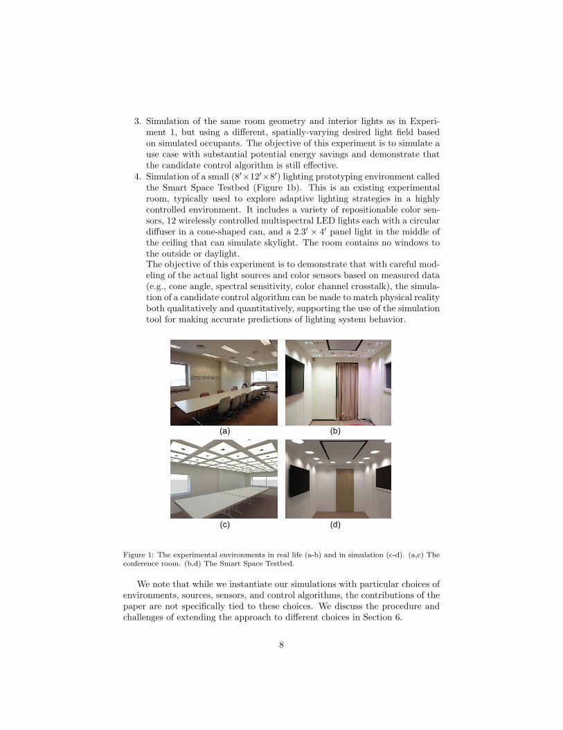
3. Simulation of the same room geometry and interior lights as in Experi-ment 1, but using a different, spatially-varying desired light field basedon simulated occupants. The objective of this experiment is to simulate ause case with substantial potential energy savings and demonstrate thatthe candidate control algorithm is still effective.

4. Simulation of a small (8′×12′×8′) lighting prototyping environment calledthe Smart Space Testbed (Figure 1b). This is an existing experimentalroom, typically used to explore adaptive lighting strategies in a highlycontrolled environment. It includes a variety of repositionable color sen-sors, 12 wirelessly controlled multispectral LED lights each with a circulardiffuser in a cone-shaped can, and a 2.3′ × 4′ panel light in the middle ofthe ceiling that can simulate skylight. The room contains no windows tothe outside or daylight.The objective of this experiment is to demonstrate that with careful mod-eling of the actual light sources and color sensors based on measured data(e.g., cone angle, spectral sensitivity, color channel crosstalk), the simula-tion of a candidate control algorithm can be made to match physical realityboth qualitatively and quantitatively, supporting the use of the simulationtool for making accurate predictions of lighting system behavior.

(a) (b)

(c) (d)

Figure 1: The experimental environments in real life (a-b) and in simulation (c-d). (a,c) Theconference room. (b,d) The Smart Space Testbed.

We note that while we instantiate our simulations with particular choices ofenvironments, sources, sensors, and control algorithms, the contributions of thepaper are not specifically tied to these choices. We discuss the procedure andchallenges of extending the approach to different choices in Section 6.

8

4. Methodology

In this section, we describe our proposed methodology for pre-visualizinglighting controller behavior in a specific space. Section 4.1 discusses our ap-proach to simulating the space, using both an offline process to generate ray-traced lightmaps and an online process to visualize the controller behavior.Section 4.2 summarizes the controller used in this study, previously proposedin [37]. Finally, Section 4.3 describes how the simulation and controller areintegrated into a common framework.

4.1. Simulation ToolsAs discussed in Section 2.1, the software tools Maya, 3ds Max Design, and

Unity Pro all play a role in our simulation framework. We chose Maya for itsability to realistically simulate lighting panels with area lights that evenly emitphotons from the panel using the mental ray plugin. 3ds Max Design has a supe-rior daylight system that allows the specification of weather data, geographicallocation, date, and time. It also uses portal lights for global illumination, whichallow the sun and sky light from windows to stream into the room. Unity Pro iswell-suited to changing environments, importing external data, and measuringand controlling objects’ properties in real time with scripting, making it an ideallighting controller simulation platform.

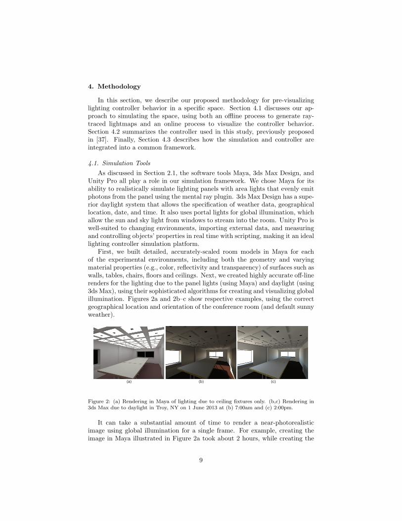
First, we built detailed, accurately-scaled room models in Maya for eachof the experimental environments, including both the geometry and varyingmaterial properties (e.g., color, reflectivity and transparency) of surfaces such aswalls, tables, chairs, floors and ceilings. Next, we created highly accurate off-linerenders for the lighting due to the panel lights (using Maya) and daylight (using3ds Max), using their sophisticated algorithms for creating and visualizing globalillumination. Figures 2a and 2b–c show respective examples, using the correctgeographical location and orientation of the conference room (and default sunnyweather).

(a) (b) (c)

Figure 2: (a) Rendering in Maya of lighting due to ceiling fixtures only. (b,c) Rendering in3ds Max due to daylight in Troy, NY on 1 June 2013 at (b) 7:00am and (c) 2:00pm.

It can take a substantial amount of time to render a near-photorealisticimage using global illumination for a single frame. For example, creating theimage in Maya illustrated in Figure 2a took about 2 hours, while creating the

9

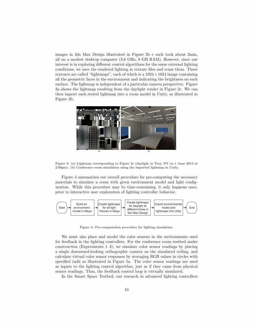
images in 3ds Max Design illustrated in Figure 2b–c each took about 2min,all on a modest desktop computer (3.6 GHz, 8 GB RAM). However, since ourinterest is in exploring different control algorithms for the same external lightingconditions, we save the rendered lighting in texture files and reuse them. Thesetextures are called “lightmaps”, each of which is a 1024×1024 image containingall the geometric faces in the environment and indicating the brightness on eachsurface. The lightmap is independent of a particular camera perspective. Figure3a shows the lightmap resulting from the daylight render in Figure 2c. We canthen import each stored lightmap into a room model in Unity, as illustrated inFigure 3b.

(a) (b)

Figure 3: (a) Lightmap corresponding to Figure 2c (daylight in Troy, NY on 1 June 2013 at2:00pm). (b) Conference room simulation using the imported lightmap in Unity.

Figure 4 summarizes our overall procedure for pre-computing the necessarymaterials to simulate a room with given environment model and light config-uration. While this procedure may be time-consuming, it only happens once,prior to interactive user exploration of lighting controller behavior.

StartBuild an

environment model in Maya

End

Create lightmaps for all light

fixtures in Maya

Create lightmapsfor daylight at

different times in3ds Max Design

Import environmental model and

lightmaps into Unity

Figure 4: Pre-computation procedure for lighting simulation.

We must also place and model the color sensors in the environments usedfor feedback in the lighting controllers. For the conference room testbed underconstruction (Experiments 1–3), we simulate color sensor readings by placinga single downward-looking orthographic camera on the simulated ceiling, andcalculate virtual color sensor responses by averaging RGB values in circles withspecified radii as illustrated in Figure 5a. The color sensor readings are usedas inputs to the lighting control algorithm, just as if they came from physicalsensor readings. Thus, the feedback control loop is virtually simulated.

In the Smart Space Testbed, our research in advanced lighting controllers

10

(a) (b)

perspective camerasorthographic camera

Figure 5: (a) In Experiments 1–3, color sensors are simulated by averaging colors in an imagefrom a single orthographic camera. (b) In Experiment 4, we more accurately simulate colorsensors using images from several perspective cameras.

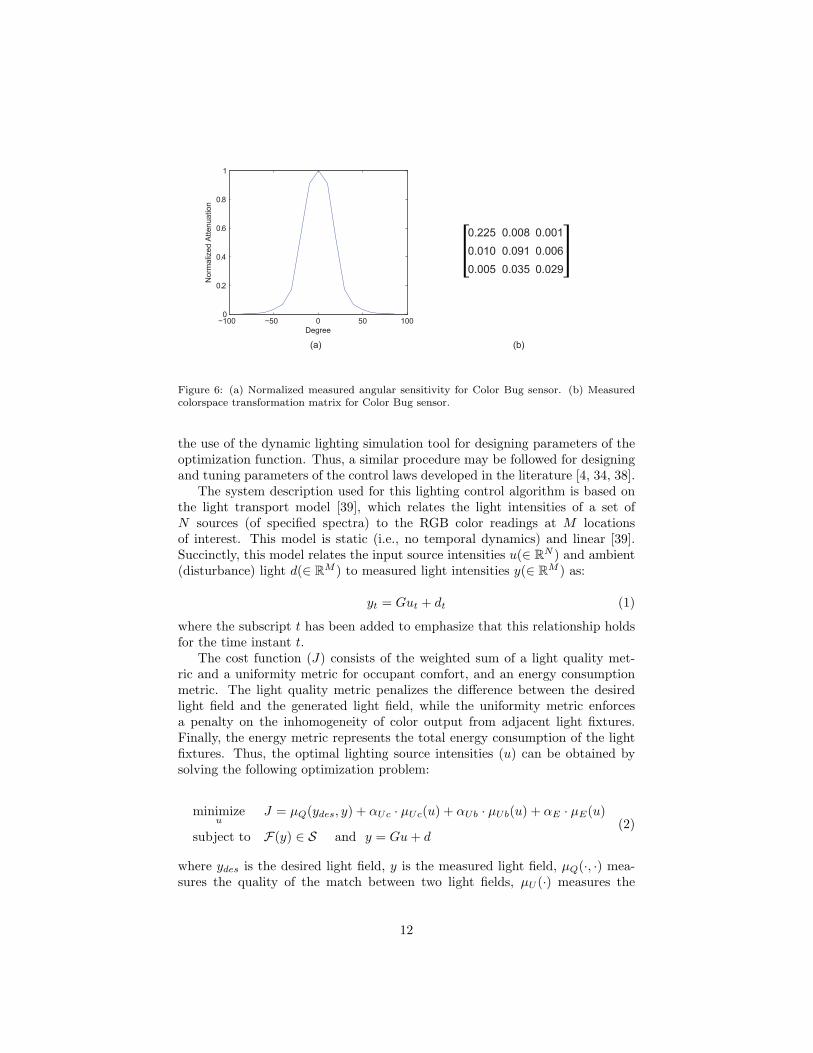
uses repositionable Seachanger wireless “Color Bug” sensors to measure localRGB intensity and illuminance. Our goal in Experiment 4 is to approximatethe true responses from these sensors as closely as possible in the simulation,which we refer to as calibration. To build an accurate model, we measured theangular sensitivity of a Color Bug using a spectroradiometer from −90◦ to 90◦

in 10◦ increments, as illustrated in Figure 6a. The sensors in the simulationfor Experiment 4 are modeled using downward-pointed perspective cameras,slightly offset from the light sources, whose resulting images are filtered withthe measured angular sensitivity profile to produce a single RGB reading persensor, as illustrated in Figure 5b.

We also noticed that the RGB colorspaces of the Color Bug and the LEDlights in the room were different, requiring a transformation in the simulation tomap the lightmap values into the correct sensor readings. We modeled this as alinear transformation, which we fitted with least-squares optimization using themeasured data from the real sources and sensors. The resulting 3 × 3 matrix,which multiplies RGB values from the lightmaps to produce RGB values of thesimulated sensors, is given in Figure 6b.

4.2. Lighting Control DesignIn this section, we present an application of the simulation tool for enabling

design iterations for a feedback control algorithm. The optimal lighting feedbackcontrol design problem is defined as determining the intensities of light sourcesto minimize an objective function, such as the one developed in [37]. Thedetermination of the optimum of this cost function in the presence of modelinguncertainty, evolving ambient light disturbances, and feedback measurementnoise is the crux of the lighting control algorithm.

It is key to note that while the design process here is directed towards thecontrol law developed in [37], the primary contribution of this manuscript is

11

−100 −50 0 50 1000

0.2

0.4

0.6

0.8

1

Degree

Nor

mal

ized

Atte

nuat

ion

(a) (b)

0.225 0.008 0.0010.010 0.091 0.0060.005 0.035 0.029

Figure 6: (a) Normalized measured angular sensitivity for Color Bug sensor. (b) Measuredcolorspace transformation matrix for Color Bug sensor.

the use of the dynamic lighting simulation tool for designing parameters of theoptimization function. Thus, a similar procedure may be followed for designingand tuning parameters of the control laws developed in the literature [4, 34, 38].

The system description used for this lighting control algorithm is based onthe light transport model [39], which relates the light intensities of a set ofN sources (of specified spectra) to the RGB color readings at M locationsof interest. This model is static (i.e., no temporal dynamics) and linear [39].Succinctly, this model relates the input source intensities u(∈ RN ) and ambient(disturbance) light d(∈ RM ) to measured light intensities y(∈ RM ) as:

yt = Gut + dt (1)

where the subscript t has been added to emphasize that this relationship holdsfor the time instant t.

The cost function (J) consists of the weighted sum of a light quality met-ric and a uniformity metric for occupant comfort, and an energy consumptionmetric. The light quality metric penalizes the difference between the desiredlight field and the generated light field, while the uniformity metric enforcesa penalty on the inhomogeneity of color output from adjacent light fixtures.Finally, the energy metric represents the total energy consumption of the lightfixtures. Thus, the optimal lighting source intensities (u) can be obtained bysolving the following optimization problem:

minimizeu

J = µQ(ydes, y) + αUc · µUc(u) + αUb · µUb(u) + αE · µE(u)

subject to F(y) ∈ S and y = Gu+ d(2)

where ydes is the desired light field, y is the measured light field, µQ(·, ·) mea-sures the quality of the match between two light fields, µU (·) measures the

12

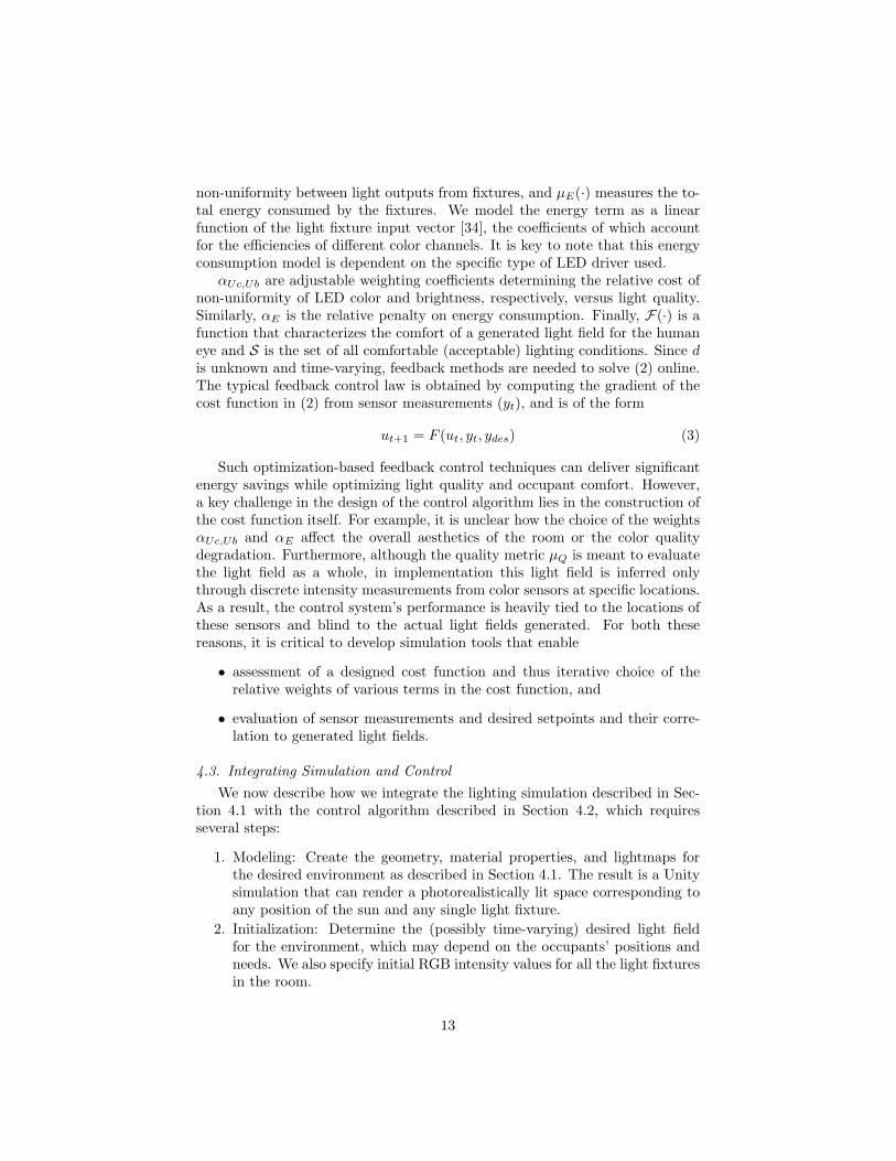
non-uniformity between light outputs from fixtures, and µE(·) measures the to-tal energy consumed by the fixtures. We model the energy term as a linearfunction of the light fixture input vector [34], the coefficients of which accountfor the efficiencies of different color channels. It is key to note that this energyconsumption model is dependent on the specific type of LED driver used.

αUc,Ub are adjustable weighting coefficients determining the relative cost ofnon-uniformity of LED color and brightness, respectively, versus light quality.Similarly, αE is the relative penalty on energy consumption. Finally, F(·) is afunction that characterizes the comfort of a generated light field for the humaneye and S is the set of all comfortable (acceptable) lighting conditions. Since dis unknown and time-varying, feedback methods are needed to solve (2) online.The typical feedback control law is obtained by computing the gradient of thecost function in (2) from sensor measurements (yt), and is of the form

ut+1 = F (ut, yt, ydes) (3)

Such optimization-based feedback control techniques can deliver significantenergy savings while optimizing light quality and occupant comfort. However,a key challenge in the design of the control algorithm lies in the construction ofthe cost function itself. For example, it is unclear how the choice of the weightsαUc,Ub and αE affect the overall aesthetics of the room or the color qualitydegradation. Furthermore, although the quality metric µQ is meant to evaluatethe light field as a whole, in implementation this light field is inferred onlythrough discrete intensity measurements from color sensors at specific locations.As a result, the control system’s performance is heavily tied to the locations ofthese sensors and blind to the actual light fields generated. For both thesereasons, it is critical to develop simulation tools that enable

• assessment of a designed cost function and thus iterative choice of therelative weights of various terms in the cost function, and

• evaluation of sensor measurements and desired setpoints and their corre-lation to generated light fields.

4.3. Integrating Simulation and ControlWe now describe how we integrate the lighting simulation described in Sec-

tion 4.1 with the control algorithm described in Section 4.2, which requiresseveral steps:

1. Modeling: Create the geometry, material properties, and lightmaps forthe desired environment as described in Section 4.1. The result is a Unitysimulation that can render a photorealistically lit space corresponding toany position of the sun and any single light fixture.

2. Initialization: Determine the (possibly time-varying) desired light fieldfor the environment, which may depend on the occupants’ positions andneeds. We also specify initial RGB intensity values for all the light fixturesin the room.

13

3. Light rendering: Combine the precomputed lightmaps to render the roomlighting corresponding to the sun position and specified fixture intensities.

4. Color sensor reading: Calculate synthetic color sensor readings by averag-ing RGB values from downward-looking cameras in the lit environment.

5. Lighting control: Input the color sensor readings to the control algorithmalong with the desired light field to update the RGB intensity values forall the light fixtures.

6. Looping: return to Step 3.

We elaborate on Step 3. In Section 4.1 we discussed how the lightmapsdue to each individual fixture and sun position are precomputed and stored.Since light transport is linear, we use superposition to create a composite lightfield out of these pre-rendered lightmaps to create an accurate lightmap for anycombination of sun position and RGB values for each fixture.

In particular, suppose there are M color sensors, N light fixtures and T dif-ferent sun positions. For each of the N fixtures, we set the RGB color to [1, 0, 0],[0, 1, 0], and [0, 0, 1] (i.e., full red, green, and blue), render global illuminationresults for each channel, and collect the 3M × 1 vector of color sensor readingsfor this scene (with no daylight). The color sensor readings due to each fixtureare collected into a 3M × 3N matrix denoted C. Similarly, for each of the Tsun positions, we compute the 3M × 1 vector, denoted dt, corresponding to thecolor sensor readings at time t for this scene (with no fixture lighting).

Thus, when the RGB values of each light determined by the control algorithmat time t are specified by a 3N × 1 vector ut, we calculate the corresponding3M × 1 color sensor reading yt as:

yt = C · ut + dt (4)

We note this process is immediate, and generates accurate color sensor read-ings for any sun/fixture configuration even though the corresponding scene isnever actually rendered. Thus, even though it may take several minutes orhours to render all the basis colormap images and collect color sensor readings(i.e., C and {dt}), the input-output relationship in the control loop is simply alow-dimensional matrix-vector product, allowing rapid exploration of differentcontrol strategies for a given space.

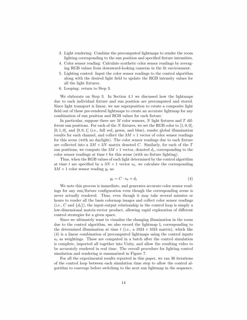
Since we ultimately want to visualize the changing illumination in the roomdue to the control algorithm, we also record the lightmap lt corresponding tothe determined illumination at time t (i.e., a 1024 × 1024 matrix), which like(4) is a linear combination of precomputed lightmaps using the control inputsut as weightings. These are computed in a batch after the control simulationis complete, imported all together into Unity, and allow the resulting video tobe accurately rendered in real time. The overall procedure for lighting controlsimulation and rendering is summarized in Figure 7.

For all the experimental results reported in this paper, we ran 30 iterationsof the control loop between each simulation time step to allow the control al-gorithm to converge before switching to the next sun lightmap in the sequence.

14

Start

Update lights with control algorithm

Done?Combine lightmapsNoYesLoad lightmaps into

Unity room model and render movie

End

Combine color sensor readings

Create basis lightmaps Initialize lights

Figure 7: Procedure of real-time simulation with lighting control.

Convergence of the control algorithm from initial color sensor readings of [0, 0, 0]only takes a few seconds of real time. Therefore, it is reasonable to assumetime-scale separation of the action of the control algorithm and the change inthe ambient sunlight pattern.

5. Experimental Results

In this section, we discuss the results of visualizing and tuning the lightingcontroller behavior through a sequence of design iterations in the four experi-ments introduced in Section 3.

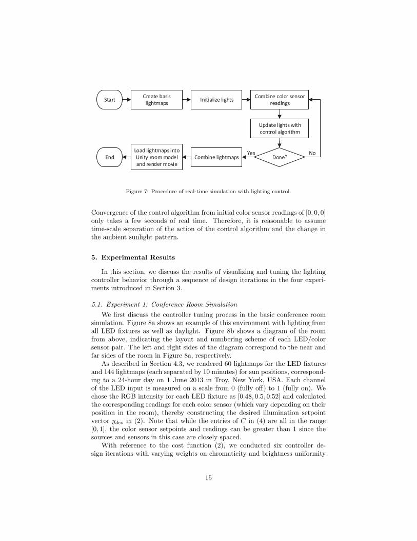
5.1. Experiment 1: Conference Room SimulationWe first discuss the controller tuning process in the basic conference room

simulation. Figure 8a shows an example of this environment with lighting fromall LED fixtures as well as daylight. Figure 8b shows a diagram of the roomfrom above, indicating the layout and numbering scheme of each LED/colorsensor pair. The left and right sides of the diagram correspond to the near andfar sides of the room in Figure 8a, respectively.

As described in Section 4.3, we rendered 60 lightmaps for the LED fixturesand 144 lightmaps (each separated by 10 minutes) for sun positions, correspond-ing to a 24-hour day on 1 June 2013 in Troy, New York, USA. Each channelof the LED input is measured on a scale from 0 (fully off) to 1 (fully on). Wechose the RGB intensity for each LED fixture as [0.48, 0.5, 0.52] and calculatedthe corresponding readings for each color sensor (which vary depending on theirposition in the room), thereby constructing the desired illumination setpointvector ydes in (2). Note that while the entries of C in (4) are all in the range[0, 1], the color sensor setpoints and readings can be greater than 1 since thesources and sensors in this case are closely spaced.

With reference to the cost function (2), we conducted six controller de-sign iterations with varying weights on chromaticity and brightness uniformity

15

(a) (b)

1

5

6

604535432

26 56

10

33

Figure 8: The configuration of Experiment 1. (a) Conference room simulation with lightingfrom LED panels and daylight. (b) Diagram of the room from above indicating light/panellayout.

(αUc,Ub), and energy usage (αE). In practice, the iterations were separated byseveral days as the results were discussed and the objective function modifiedto produce controller behavior deemed to be desirable. The iterations are asfollows, described in further detail below:

• Exp-1a: No disturbance, no weighting on energy (αE = 0)

• Exp-1b: No disturbance, energy weighting αE = 0.1

• Exp-1c: With disturbance, αE = 0

• Exp-1d: With disturbance, αE = 0, weight 1 on chromaticity uniformity(αUc).

• Exp-1e: With disturbance, αE = 0, αUc = 1 and varying weights 0.001,0.01, 0.1 and 1 on intensity uniformity (αUb).

• Exp-1f: With disturbance, αE = 0.1, αUc = 1 and αUb = 0.001.

We first considered an empty room with no external disturbance from sun-light. The initial condition was a darkened room with all light fixture intensitiesset to [0.1, 0.1, 0.1]. In Exp-1a, we observed the lights quickly converging to thesetpoint. When a weight on energy usage is added (Exp-1b), the illuminationin the room at convergence is somewhat darker and the fidelity of the desiredsetpoint is compromised, as would be expected. After convergence, the inputsto LED-35 in Exp-1a and Exp-1b are [0.48, 0.5, 0.52] and [0.35, 0.4, 0.42], re-spectively. On the other hand, the energy usage in Exp-1b was 78% of thatin Exp-1a. These results mirror what occurs when the control algorithm isimplemented in a physical environment (see Section 5.4 and [37]).

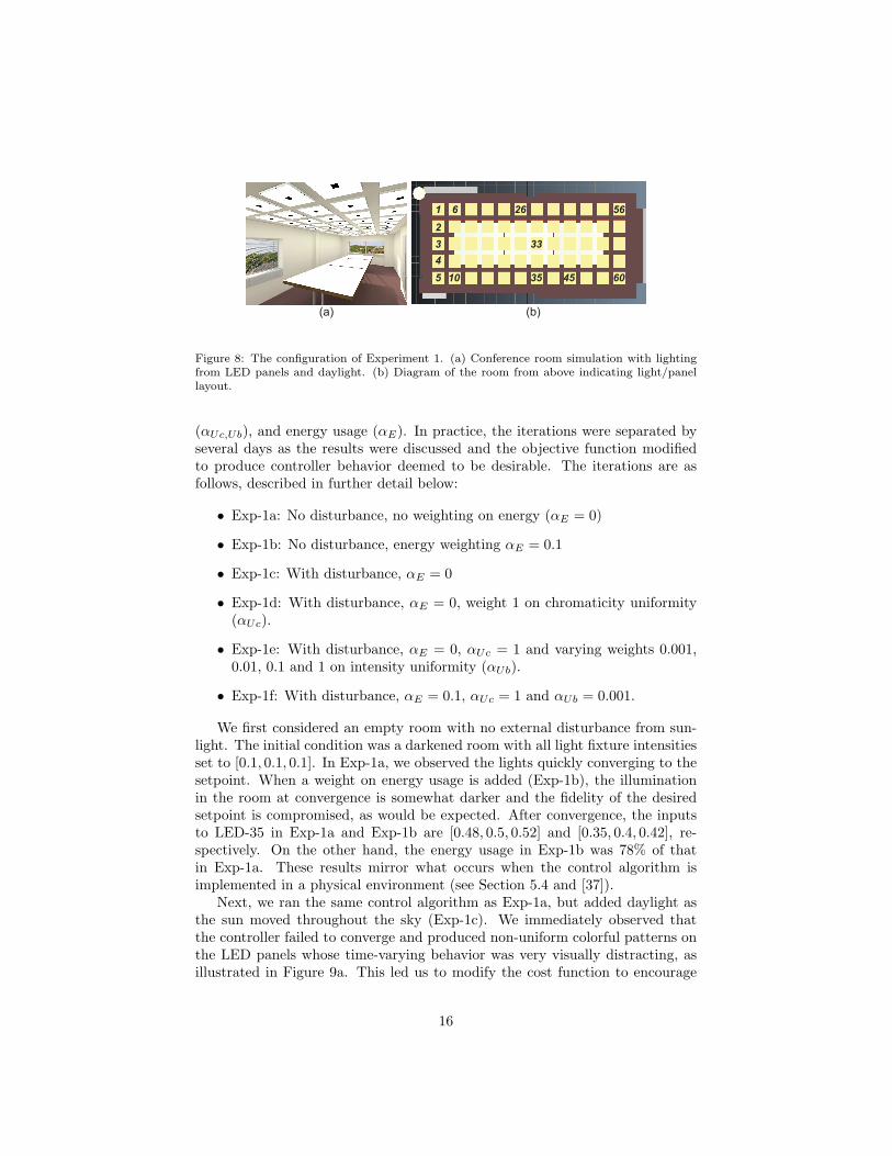
Next, we ran the same control algorithm as Exp-1a, but added daylight asthe sun moved throughout the sky (Exp-1c). We immediately observed thatthe controller failed to converge and produced non-uniform colorful patterns onthe LED panels whose time-varying behavior was very visually distracting, asillustrated in Figure 9a. This led us to modify the cost function to encourage

16

uniformity in chromaticity by setting αUc to 1 in (2) (Exp-1d). The results areillustrated in Figure 9b. The panels are no longer randomly colored (that is,the uniformity term forces the R, G, and B channels to be almost identical forevery fixture). However, the intensities of neighboring lights still differ sharplyand can change quickly, which is still very visually distracting.

(a) (b)

0 4 8 12 16 20 240

0.5

1

1.5

2LED−35

Col

or S

enso

r Rea

ding

0 4 8 12 16 20 240

0.25

0.5

0.75

1

LED

Inpu

t

Time (hour)

0 4 8 12 16 20 240

0.5

1

1.5

2LED−35

Col

or S

enso

r Rea

ding

0 4 8 12 16 20 240

0.25

0.5

0.75

1

LED

Inpu

t

Time (hour)

Figure 9: Control results for (a) Exp-1c and (b) Exp-1d, Top: visualizations of the room at7:00am. Middle: color reading from sensor 35. Bottom: color LED input.

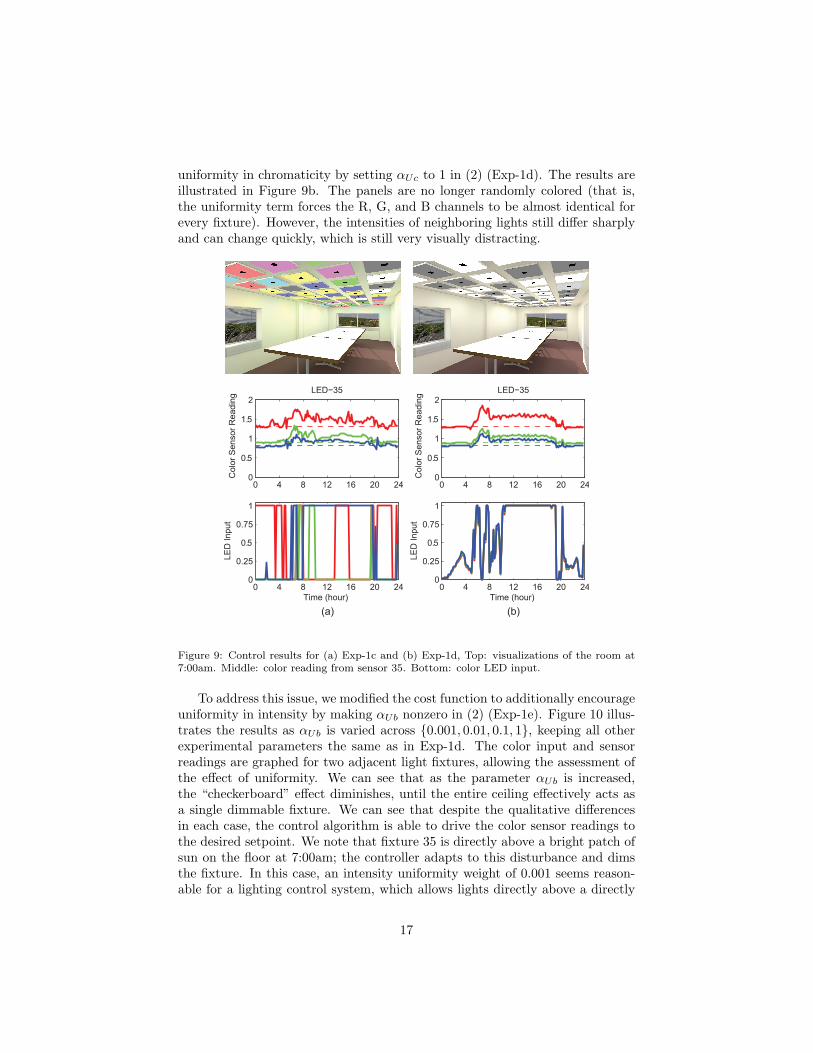
To address this issue, we modified the cost function to additionally encourageuniformity in intensity by making αUb nonzero in (2) (Exp-1e). Figure 10 illus-trates the results as αUb is varied across {0.001, 0.01, 0.1, 1}, keeping all otherexperimental parameters the same as in Exp-1d. The color input and sensorreadings are graphed for two adjacent light fixtures, allowing the assessment ofthe effect of uniformity. We can see that as the parameter αUb is increased,the “checkerboard” effect diminishes, until the entire ceiling effectively acts asa single dimmable fixture. We can see that despite the qualitative differencesin each case, the control algorithm is able to drive the color sensor readings tothe desired setpoint. We note that fixture 35 is directly above a bright patch ofsun on the floor at 7:00am; the controller adapts to this disturbance and dimsthe fixture. In this case, an intensity uniformity weight of 0.001 seems reason-able for a lighting control system, which allows lights directly above a directly

17

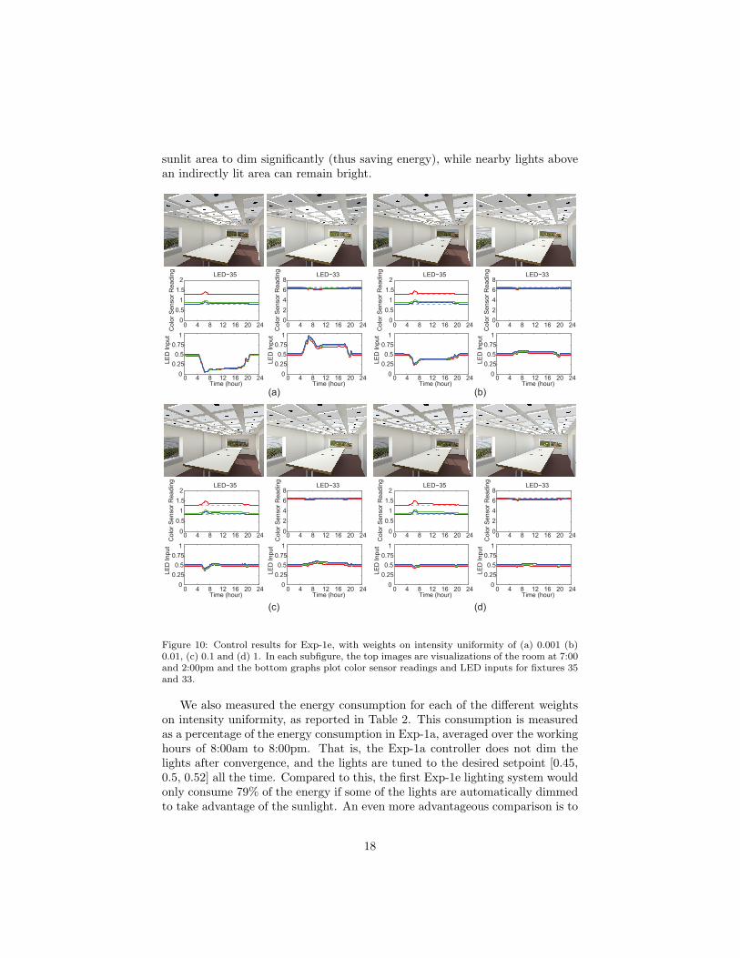
sunlit area to dim significantly (thus saving energy), while nearby lights abovean indirectly lit area can remain bright.

(a) (b)

(c) (d)

0 4 8 12 16 20 240

0.51

1.52

LED−35

Col

or S

enso

r Rea

ding

0 4 8 12 16 20 2400.250.5

0.751

LED

Inpu

t

Time (hour)

0 4 8 12 16 20 2402468

LED−33C

olor

Sen

sor R

eadi

ng

0 4 8 12 16 20 2400.250.5

0.751

LED

Inpu

t

Time (hour)

0 4 8 12 16 20 2402468

LED−33

Col

or S

enso

r Rea

ding

0 4 8 12 16 20 2400.250.5

0.751

LED

Inpu

t

Time (hour)

0 4 8 12 16 20 240

0.51

1.52

LED−35

Col

or S

enso

r Rea

ding

0 4 8 12 16 20 2400.250.5

0.751

LED

Inpu

tTime (hour)

0 4 8 12 16 20 240

0.51

1.52

LED−35

Col

or S

enso

r Rea

ding

0 4 8 12 16 20 240

0.250.5

0.751

LED

Inpu

t

Time (hour)

0 4 8 12 16 20 240

2468

LED−33

Col

or S

enso

r Rea

ding

0 4 8 12 16 20 240

0.250.5

0.751

LED

Inpu

t

Time (hour)

0 4 8 12 16 20 240

2468

LED−33C

olor

Sen

sor R

eadi

ng

0 4 8 12 16 20 240

0.250.5

0.751

LED

Inpu

t

Time (hour)

0 4 8 12 16 20 240

0.51

1.52

LED−35

Col

or S

enso

r Rea

ding

0 4 8 12 16 20 240

0.250.5

0.751

LED

Inpu

t

Time (hour)

Figure 10: Control results for Exp-1e, with weights on intensity uniformity of (a) 0.001 (b)0.01, (c) 0.1 and (d) 1. In each subfigure, the top images are visualizations of the room at 7:00and 2:00pm and the bottom graphs plot color sensor readings and LED inputs for fixtures 35and 33.

We also measured the energy consumption for each of the different weightson intensity uniformity, as reported in Table 2. This consumption is measuredas a percentage of the energy consumption in Exp-1a, averaged over the workinghours of 8:00am to 8:00pm. That is, the Exp-1a controller does not dim thelights after convergence, and the lights are tuned to the desired setpoint [0.45,0.5, 0.52] all the time. Compared to this, the first Exp-1e lighting system wouldonly consume 79% of the energy if some of the lights are automatically dimmedto take advantage of the sunlight. An even more advantageous comparison is to

18

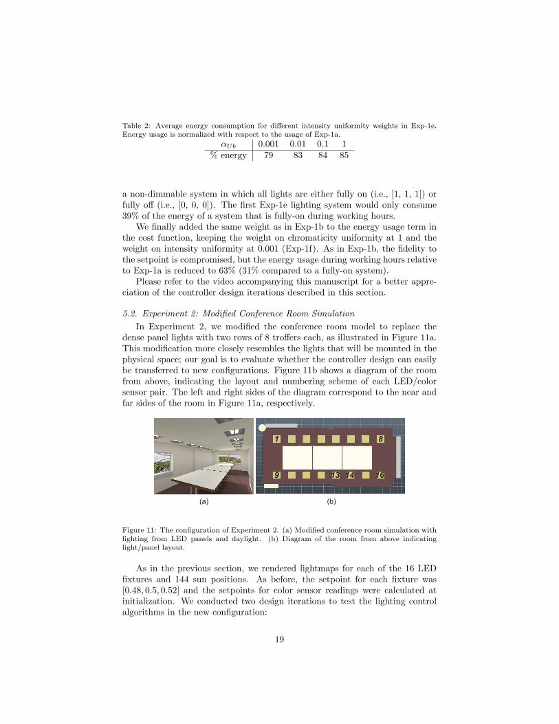
Table 2: Average energy consumption for different intensity uniformity weights in Exp-1e.Energy usage is normalized with respect to the usage of Exp-1a.

αUb 0.001 0.01 0.1 1% energy 79 83 84 85

a non-dimmable system in which all lights are either fully on (i.e., [1, 1, 1]) orfully off (i.e., [0, 0, 0]). The first Exp-1e lighting system would only consume39% of the energy of a system that is fully-on during working hours.

We finally added the same weight as in Exp-1b to the energy usage term inthe cost function, keeping the weight on chromaticity uniformity at 1 and theweight on intensity uniformity at 0.001 (Exp-1f). As in Exp-1b, the fidelity tothe setpoint is compromised, but the energy usage during working hours relativeto Exp-1a is reduced to 63% (31% compared to a fully-on system).

Please refer to the video accompanying this manuscript for a better appre-ciation of the controller design iterations described in this section.

5.2. Experiment 2: Modified Conference Room SimulationIn Experiment 2, we modified the conference room model to replace the

dense panel lights with two rows of 8 troffers each, as illustrated in Figure 11a.This modification more closely resembles the lights that will be mounted in thephysical space; our goal is to evaluate whether the controller design can easilybe transferred to new configurations. Figure 11b shows a diagram of the roomfrom above, indicating the layout and numbering scheme of each LED/colorsensor pair. The left and right sides of the diagram correspond to the near andfar sides of the room in Figure 11a, respectively.

(a) (b)

1

13

8

9 1614

Figure 11: The configuration of Experiment 2. (a) Modified conference room simulation withlighting from LED panels and daylight. (b) Diagram of the room from above indicatinglight/panel layout.

As in the previous section, we rendered lightmaps for each of the 16 LEDfixtures and 144 sun positions. As before, the setpoint for each fixture was[0.48, 0.5, 0.52] and the setpoints for color sensor readings were calculated atinitialization. We conducted two design iterations to test the lighting controlalgorithms in the new configuration:

19

• Exp-2a: With disturbance, no weighting on energy (αE = 0), weight onchromaticity uniformity αUc = 1, weight on intensity uniformity αUb =0.001.

• Exp-2b: With disturbance, αE = 0, αUc = 1 and αUb = 0.05.

Exp-2a is directly comparable to Exp-1e from Experiment 1; the experimen-tal results are illustrated in Figure 12 for two times of day and two adjacentfixtures. As before, the controller succeeded with dimming a fixture (LED-14)above a bright patch of sunlight, but an adjacent fixture (LED-13) was bright-ened to achieve the desired color sensor readings, leading to a perceptuallydistracting non-uniformity between nearby lights.

(a) (b)

0 4 8 12 16 20 240

0.25

0.5

0.75

1LED−14

Col

or S

enso

r Rea

ding

0 4 8 12 16 20 240

0.25

0.5

0.75

1

LED

Inpu

t

Time (hour)

0 4 8 12 16 20 240

0.25

0.5

0.75

1LED−13

Col

or S

enso

r Rea

ding

0 4 8 12 16 20 240

0.25

0.5

0.75

1

LED

Inpu

t

Time (hour)

Figure 12: Control results for Exp-2a. Top: visualizations of the room at (left) 7:00 and(right) 2:00pm. Bottom: color sensor readings and LED inputs for adjacent fixtures (left) 14and (right) 13.

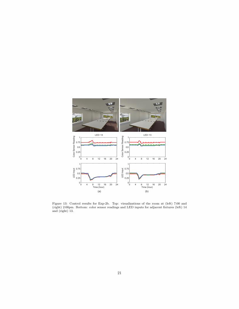
We therefore increased the weighting on intensity uniformity to 0.05 (Exp-2b); the experimental results are illustrated in Figure 13. Compared with Figure12, we can see the lights are more uniform as desired.

The energy consumptions (averaged as before over daylight hours and nor-malized with respect to the converged LED inputs without disturbance) for thetwo experiments were 50% and 55% for Exp-2a and Exp-2b, respectively.

20

(a) (b)

0 4 8 12 16 20 240

0.25

0.5

0.75

1LED−13

Col

or S

enso

r Rea

ding

0 4 8 12 16 20 240

0.25

0.5

0.75

1

LED

Inpu

t

Time (hour)

0 4 8 12 16 20 240

0.25

0.5

0.75

1LED−14

Col

or S

enso

r Rea

ding

0 4 8 12 16 20 240

0.25

0.5

0.75

1

LED

Inpu

t

Time (hour)

Figure 13: Control results for Exp-2b. Top: visualizations of the room at (left) 7:00 and(right) 2:00pm. Bottom: color sensor readings and LED inputs for adjacent fixtures (left) 14and (right) 13.

21

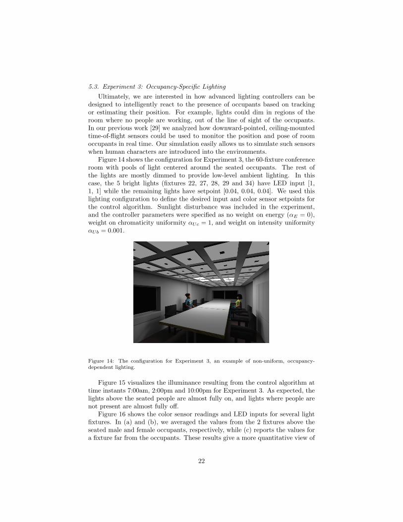
5.3. Experiment 3: Occupancy-Specific LightingUltimately, we are interested in how advanced lighting controllers can be

designed to intelligently react to the presence of occupants based on trackingor estimating their position. For example, lights could dim in regions of theroom where no people are working, out of the line of sight of the occupants.In our previous work [29] we analyzed how downward-pointed, ceiling-mountedtime-of-flight sensors could be used to monitor the position and pose of roomoccupants in real time. Our simulation easily allows us to simulate such sensorswhen human characters are introduced into the environments.

Figure 14 shows the configuration for Experiment 3, the 60-fixture conferenceroom with pools of light centered around the seated occupants. The rest ofthe lights are mostly dimmed to provide low-level ambient lighting. In thiscase, the 5 bright lights (fixtures 22, 27, 28, 29 and 34) have LED input [1,1, 1] while the remaining lights have setpoint [0.04, 0.04, 0.04]. We used thislighting configuration to define the desired input and color sensor setpoints forthe control algorithm. Sunlight disturbance was included in the experiment,and the controller parameters were specified as no weight on energy (αE = 0),weight on chromaticity uniformity αUc = 1, and weight on intensity uniformityαUb = 0.001.

Figure 14: The configuration for Experiment 3, an example of non-uniform, occupancy-dependent lighting.

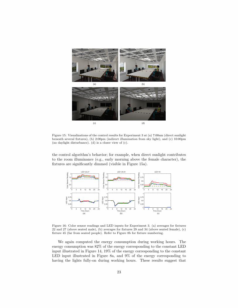
Figure 15 visualizes the illuminance resulting from the control algorithm attime instants 7:00am, 2:00pm and 10:00pm for Experiment 3. As expected, thelights above the seated people are almost fully on, and lights where people arenot present are almost fully off.

Figure 16 shows the color sensor readings and LED inputs for several lightfixtures. In (a) and (b), we averaged the values from the 2 fixtures above theseated male and female occupants, respectively, while (c) reports the values fora fixture far from the occupants. These results give a more quantitative view of

22

(a) (b)

(c) (d)

Figure 15: Visualizations of the control results for Experiment 3 at (a) 7:00am (direct sunlightbeneath several fixtures), (b) 2:00pm (indirect illumination from sky light), and (c) 10:00pm(no daylight disturbance). (d) is a closer view of (c).

the control algorithm’s behavior; for example, when direct sunlight contributesto the room illuminance (e.g., early morning above the female character), thefixtures are significantly dimmed (visible in Figure 15a).

(a) (c)(b)

0 4 8 12 16 20 240

0.5

1

1.5

2

Col

or S

enso

r Rea

ding

LED−22,27

0 4 8 12 16 20 240

0.25

0.5

0.75

1

LED

Inpu

t

Time (hour)

0 4 8 12 16 20 240

0.5

1

1.5

2

Col

or S

enso

r Rea

ding

LED−29,34

0 4 8 12 16 20 240

0.25

0.5

0.75

1

LED

Inpu

t

Time (hour)

0 4 8 12 16 20 240

0.25

0.5

0.75

1LED−45

Col

or S

enso

r Rea

ding

0 4 8 12 16 20 240

0.25

0.5

0.75

1

LED

Inpu

t

Time (hour)

Figure 16: Color sensor readings and LED inputs for Experiment 3. (a) averages for fixtures22 and 27 (above seated male), (b) averages for fixtures 29 and 34 (above seated female), (c)fixture 45 (far from seated people). Refer to Figure 8b for fixture numbering.

We again computed the energy consumption during working hours. Theenergy consumption was 82% of the energy corresponding to the constant LEDinput illustrated in Figure 14, 19% of the energy corresponding to the constantLED input illustrated in Figure 8a, and 9% of the energy corresponding tohaving the lights fully-on during working hours. These results suggest that

23

substantial energy savings can be realized by customizing the lighting to theoccupants, as is well-known [40, 4, 41].

5.4. Experiment 4: Comparing the Real and Simulated Smart Space TestbedsFinally, Experiment 4 addresses the secondary objective of accurately match-

ing the simulation LED source and color sensor readings to a physical space.The process of calibrating the response of the actual sensors in the Smart SpaceTestbed to the actual sources was described in Section 4.1.

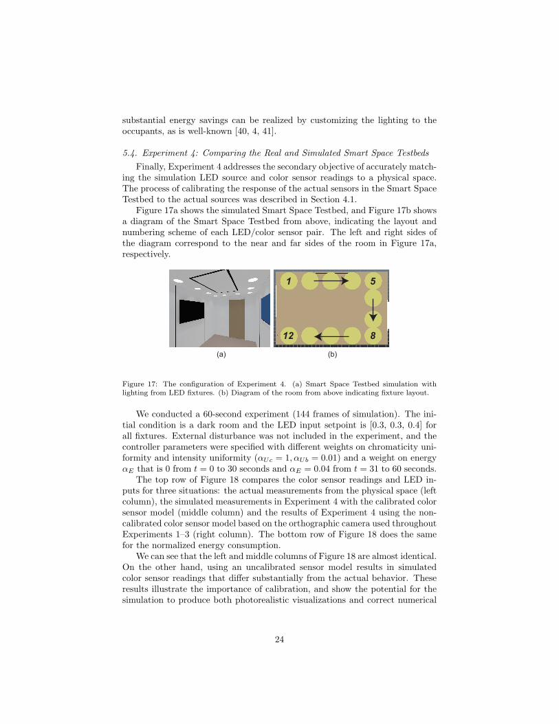
Figure 17a shows the simulated Smart Space Testbed, and Figure 17b showsa diagram of the Smart Space Testbed from above, indicating the layout andnumbering scheme of each LED/color sensor pair. The left and right sides ofthe diagram correspond to the near and far sides of the room in Figure 17a,respectively.

(a) (b)

1 5

812

Figure 17: The configuration of Experiment 4. (a) Smart Space Testbed simulation withlighting from LED fixtures. (b) Diagram of the room from above indicating fixture layout.

We conducted a 60-second experiment (144 frames of simulation). The ini-tial condition is a dark room and the LED input setpoint is [0.3, 0.3, 0.4] forall fixtures. External disturbance was not included in the experiment, and thecontroller parameters were specified with different weights on chromaticity uni-formity and intensity uniformity (αUc = 1, αUb = 0.01) and a weight on energyαE that is 0 from t = 0 to 30 seconds and αE = 0.04 from t = 31 to 60 seconds.

The top row of Figure 18 compares the color sensor readings and LED in-puts for three situations: the actual measurements from the physical space (leftcolumn), the simulated measurements in Experiment 4 with the calibrated colorsensor model (middle column) and the results of Experiment 4 using the non-calibrated color sensor model based on the orthographic camera used throughoutExperiments 1–3 (right column). The bottom row of Figure 18 does the samefor the normalized energy consumption.

We can see that the left and middle columns of Figure 18 are almost identical.On the other hand, using an uncalibrated sensor model results in simulatedcolor sensor readings that differ substantially from the actual behavior. Theseresults illustrate the importance of calibration, and show the potential for thesimulation to produce both photorealistic visualizations and correct numerical

24

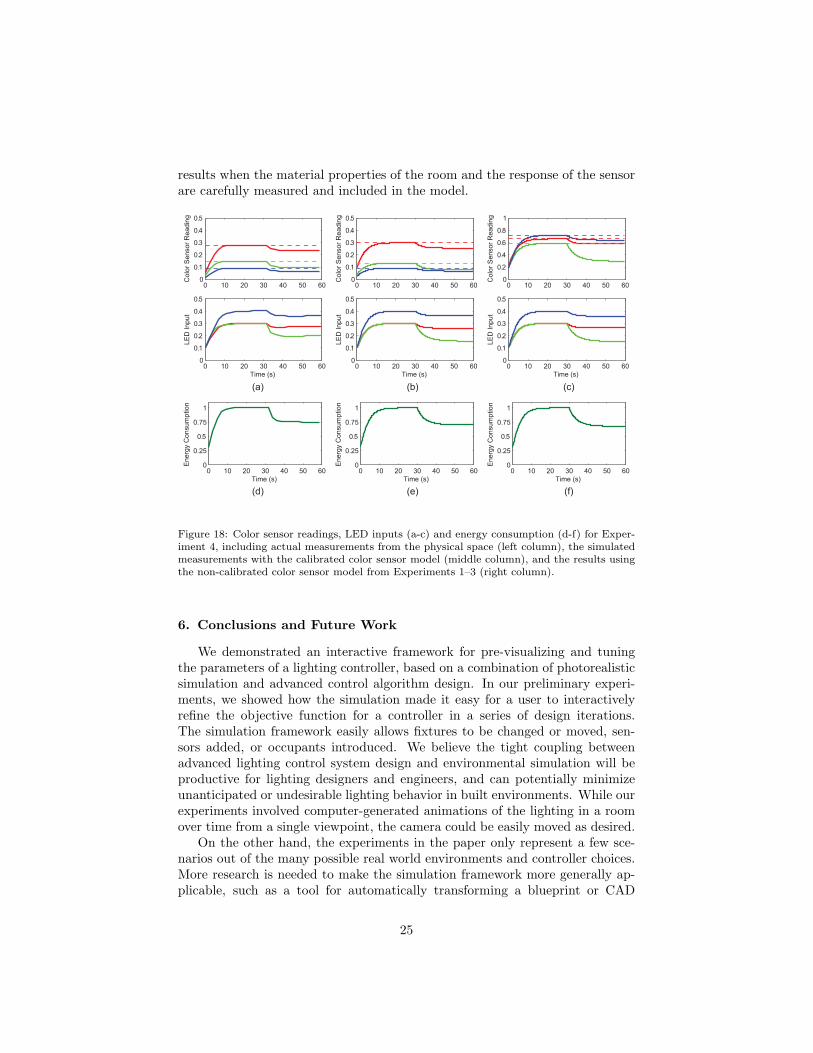
results when the material properties of the room and the response of the sensorare carefully measured and included in the model.

(c)

(d)

(a) (b)

(e) (f)

0 10 20 30 40 50 600

0.1

0.2

0.3

0.4

0.5

Col

or S

enso

r Rea

ding

0 10 20 30 40 50 600

0.1

0.2

0.3

0.4

0.5

LED

Inpu

t

Time (s)

0 10 20 30 40 50 600

0.1

0.2

0.3

0.4

0.5

Col

or S

enso

r Rea

ding

0 10 20 30 40 50 600

0.1

0.2

0.3

0.4

0.5

LED

Inpu

t

Time (s)

0 10 20 30 40 50 600

0.2

0.4

0.6

0.8

1

Col

or S

enso

r Rea

ding

0 10 20 30 40 50 600

0.1

0.2

0.3

0.4

0.5

LED

Inpu

t

Time (s)

0 10 20 30 40 50 600

0.25

0.5

0.75

1

Time (s)

Ene

rgy

Con

sum

ptio

n

0 10 20 30 40 50 600

0.25

0.5

0.75

1

Time (s) E

nerg

y C

onsu

mpt

ion

0 10 20 30 40 50 600

0.25

0.5

0.75

1

Time (s)

Ene

rgy

Con

sum

ptio

n

Figure 18: Color sensor readings, LED inputs (a-c) and energy consumption (d-f) for Exper-iment 4, including actual measurements from the physical space (left column), the simulatedmeasurements with the calibrated color sensor model (middle column), and the results usingthe non-calibrated color sensor model from Experiments 1–3 (right column).

6. Conclusions and Future Work

We demonstrated an interactive framework for pre-visualizing and tuningthe parameters of a lighting controller, based on a combination of photorealisticsimulation and advanced control algorithm design. In our preliminary experi-ments, we showed how the simulation made it easy for a user to interactivelyrefine the objective function for a controller in a series of design iterations.The simulation framework easily allows fixtures to be changed or moved, sen-sors added, or occupants introduced. We believe the tight coupling betweenadvanced lighting control system design and environmental simulation will beproductive for lighting designers and engineers, and can potentially minimizeunanticipated or undesirable lighting behavior in built environments. While ourexperiments involved computer-generated animations of the lighting in a roomover time from a single viewpoint, the camera could be easily moved as desired.

On the other hand, the experiments in the paper only represent a few sce-narios out of the many possible real world environments and controller choices.More research is needed to make the simulation framework more generally ap-plicable, such as a tool for automatically transforming a blueprint or CAD

25

model into the pre-computed geometry and lightmaps required to investigatecontroller behavior. A bigger challenge, both technical and social, is the in-sertion of lighting pre-visualization tools into the typical architectural designprocess, especially in the early phases when the choice of lighting controllermight significantly impact choices about lighting fixtures or facade elements. Infuture work, we plan to collaborate directly with architects and lighting design-ers to find ways of making the simulation framework more applicable to commonpractice.

Many research directions follow from this initial prototype. We are currentlyin the process of physically measuring light fields and transfer functions in thephysical conference room under construction, to make the simulation of thisspace even more accurate (i.e., following on from the experiments in Section5.4). We are also in the process of accurately characterizing and simulating newprototype sensors to be designed and deployed. We expect the lighting controlsimulation to inform both the development of these new sensors (e.g., necessarydirectional and spectral sensitivity) as well as the placement and characteristicsof lighting fixtures in the constructed space.

We are also exploring several directions to make the simulation more real-istic. These include moving beyond RGB sources and sensors to multispectralresponses; incorporating wall-mounted sensors or sensors not collocated with fix-tures; modeling occupant tracking with ceiling-mounted time-of-flight sensors,and exploring dynamic desired light fields (e.g., that adapt to moving occupantsor changing weather).

A key unresolved problem, well beyond the scope of this study, is that ofdeciding the “right” time-varying light field for a given environment and usecase. A control algorithm can be designed to accurately reach a desired setpoint,and simulation can do an excellent job of visualizing the results, but determiningthe setpoint itself is quite challenging. For example, the setpoint could varyaccording to the number, position, and pose of occupants, their activity (e.g.,working in small groups, holding a discussion, watching a presentation, watchinga film), and the time of day (e.g., using circadian theory to expose the occupantsto warmer colors after sunset). The situation is further complicated by thechallenges of designing a controller that can simultaneously satisfy the subjectivepreferences of multiple users, and the practical need to override the controller ifthe occupants find the result unsatisfactory [6]. Our continuing investigations inthis area will engage lighting designers to help address these difficult questions.

7. Acknowledgements

This work was supported primarily by the Engineering Research CentersProgram (ERC) of the National Science Foundation under NSF CooperativeAgreement No. EEC-0812056 and in part by New York State under NYSTARcontract C090145. Thanks to Brandon Andow for his perspectives on architec-tural and lighting design, and to the anonymous reviewer for detailed suggestionson improving the presentation of the paper.

26

References

[1] U.S. Energy Information Administration, Annual Energy Outlook 2013, DOE/EIA-0383(2013), Washington, DC (April 2013).

[2] E. S. Lee, S. E. Selkowitz, The design and evaluation of integrated envelope and lightingcontrol strategies for commercial buildings, Tech. rep., Lawrence Berkeley Lab., CA(United States) (1994).

[3] B. Roisin, M. Bodart, A. Deneyer, P. D’Herdt, Lighting energy savings in offices usingdifferent control systems and their real consumption, Energy and Buildings 40 (4) (2008)514–523.

[4] V. Singhvi, A. Krause, C. Guestrin, J. H. Garrett Jr, H. S. Matthews, Intelligent lightcontrol using sensor networks, in: Proceedings of the 3rd International Conference onEmbedded Networked Sensor Systems, 2005.

[5] M. Bodart, A. De Herde, Global energy savings in offices buildings by the use of day-lighting, Energy and Buildings 34 (5) (2002) 421–429.

[6] A. D. Galasiu, J. A. Veitch, Occupant preferences and satisfaction with the luminous en-vironment and control systems in daylit offices: a literature review, Energy and Buildings38 (7) (2006) 728–742.

[7] O. Masoso, L. Grobler, The dark side of occupants’ behaviour on building energy use,Energy and Buildings 42 (2) (2010) 173–177.

[8] Y. Sheng, T. C. Yapo, C. Young, B. Cutler, A spatially augmented reality sketchinginterface for architectural daylighting design, IEEE Transactions on Visualization andComputer Graphics 17 (1) (2011) 38–50.

[9] M. G. Figueiro, M. S. Rea, R. G. Stevens, A. C. Rea, Daylight and productivity —a possible link to circadian regulation, in: Proceedings of the Fifth International LROLighting Research Symposium, 2002.

[10] P. Boyce, C. Hunter, O. Howlett, The benefits of daylight through windows, Tech. rep.,Lighting Research Center, Rensselaer Polytechnic Institute, Troy, NY (2003).

[11] M. S. Rea, M. G. Figueiro, A. Bierman, J. D. Bullough, Circadian light, Journal ofCircadian Rhythms 8 (1) (2010) 2.

[12] E. Krietemeyer, Dynamic design framework for mediated bioresponsive building en-velopes, Ph.D. thesis, Rensselaer Polytechnic Institute, Troy, NY (2013).

[13] Y. Sheng, Interactive daylight visualization in spatially augmented reality environments,Ph.D. thesis, Rensselaer Polytechnic Institute, Troy, NY (2013).

[14] J. Clarke, Energy simulation in building design, Routledge, 2012.

[15] G. W. Larson, R. Shakespeare, C. Ehrlich, J. Mardaljevic, E. Phillips, P. Apian-Bennewitz, Rendering with Radiance: the art and science of lighting visualization, Mor-gan Kaufmann San Francisco, CA, 1998.

[16] C. Reinhart, A. Fitz, Findings from a survey on the current use of daylight simulationsin building design, Energy and Buildings 38 (7) (2006) 824–835.

[17] R. Cusson, J. Cardoso, Realistic Architectural Visualization with 3ds Max and mentalray, Focal Press, 2012.

[18] L. Lanier, Advanced Maya texturing and lighting, Sybex, 2006.

27

[19] C. Reinhart, P. F. Breton, Experimental validation of Autodesk R© 3ds Max R© Design2009 and Daysim 3.0, Leukos 6 (1) (2009) 7–35.

[20] K. Lagios, J. Niemasz, C. Reinhart, Animated building performance simulation (ABPS)–linking Rhinoceros/Grasshopper with Radiance/Daysim, in: Proceedings of SimBuild,2010.

[21] J. Mardaljevic, L. Heschong, E. Lee, Daylight metrics and energy savings, Lighting Re-search and Technology 41 (3) (2009) 261–283.

[22] C. Reinhart, J. Mardaljevic, Z. Rogers, Dynamic daylight performance metrics for sus-tainable building design, Leukos 3 (1) (2006) 1–25.

[23] C. Reinhart, J. Wienold, The daylighting dashboard — a simulation-based design analysisfor daylit spaces, Building and Environment 46 (2) (2011) 386–396.

[24] M. Andersen, S. Kleindienst, L. Yi, J. Lee, M. Bodart, B. Cutler, An intuitive daylightingperformance analysis and optimization approach, Building Research & Information 36 (6)(2008) 593–607.

[25] S. Kleindienst, M. Andersen, Comprehensive annual daylight design through a goal-basedapproach, Building Research & Information 40 (2) (2012) 154–173.

[26] S. Wang, Z. Mao, C. Zeng, H. Gong, S. Li, B. Chen, A new method of virtual realitybased on Unity3D, in: International Conference on Geoinformatics, 2010.

[27] M. Zyda, From visual simulation to virtual reality to games, Computer 38 (9) (2005)25–32.

[28] A. Indraprastha, M. Shinozaki, The investigation on using Unity3D game engine in urbandesign study, ITB Journal of Information and Communication Technology 3 (1) (2009)1–18.

[29] L. Jia, R. J. Radke, Using time-of-flight measurements for privacy-preserving tracking ina smart room, IEEE Transactions on Industrial Informatics (In Press).

[30] F. Qureshi, D. Terzopoulos, Smart camera networks in virtual reality, Proceedings of theIEEE 96 (10) (2008) 1640–1656.

[31] M. C. Mozer, The neural network house: An environment that adapts to its inhabitants,in: Proc. AAAI Spring Symp. Intelligent Environments, 1998, pp. 110–114.

[32] S. Selkowitz, E. Lee, O. Aschehoug, Perspectives on advanced facades with dynamicglazings and integrated lightings controls, in: CISBAT 2003, Innovation in BuildingEnvelopes and Environmental Systems, 2003.

[33] Y.-J. Wen, J. Granderson, A. M. Agogino, Towards embedded wireless-networked intel-ligent daylighting systems for commercial buildings, in: IEEE International Conferenceon Sensor Networks, Ubiquitous, and Trustworthy Computing, 2006.

[34] M. Aldrich, N. Zhao, J. Paradiso, Energy efficient control of polychromatic solid statelighting using a sensor network, in: Tenth International Conference on Solid State Light-ing, 2010.

[35] B. Lee, M. Aldrich, J. A. Paradiso, Methods for measuring work surface illuminance inadaptive solid state lighting networks, in: Eleventh International Conference on SolidState Lighting, 2011.

[36] S. Afshari, S. Mishra, A. Julius, F. Lizarralde, J. T. Wen, Modeling and feedback controlof color-tunable led lighting systems, in: American Control Conference (ACC), 2012,IEEE, 2012, pp. 3663–3668.

28

[37] S. Afshari, S. Mishra, A. Julius, F. Lizarralde, J. D. Wason, J. T. Wen, Modeling andcontrol of color tunable lighting systems, Energy and Buildings (In press).

[38] H. Park, J. Burke, M. B. Srivastava, Design and implementation of a wireless sensornetwork for intelligent light control, in: Proceedings of the 6th International Conferenceon Information Processing in Sensor Networks, ACM, 2007, pp. 370–379.

[39] J. Foley, A. van Dam, S. Feiner, H. J.F., Computer Graphics: Principles and Practice inC, 2nd Edition, Addison-Wesley Professional, 1995.

[40] D. Caicedo, A. Pandharipande, G. Leus, Occupancy-based illumination control of LEDlighting systems, Lighting Research and Technology 43 (2) (2011) 217–234.

[41] A. Pandharipande, D. Caicedo, Daylight integrated illumination control of LED systemsbased on enhanced presence sensing, Energy and Buildings 43 (4) (2011) 944–950.

29