Simulation Modeling: Concepts and Practice

CONTENTS

5.1 A Simple Problem: Operations at Conley Fisheries

5.2 Preliminary Analysis of Conley Fisheries

5.3 A Simulation Model of the Conley Fisheries Problem

5.4 Random Number Generators

5.5 Creating Numbers that Obey a Discrete Probability Distribution

5.6 Creating Numbers that Obey a Continuous Probability Distribution

5.7 Completing the Simulation Model of Conley Fisheries

5.8 Using the Sample Data for Analysis

5.9 Summary of Simulation Modeling, and Guidelines on the Use of Simulation

5.10 Computer Software for Simulation Modeling

5.11 Typical Uses of Simulation Models

5.12 Case Modules The Gentle Lentil Restaurant To Hedge or not to Hedge? Ontario Gateway Casterbridge Bank

THIS CHAPTER PRESENTS THE BASIC CONCEPTS AND DEMONSTRATES TI-IE MANAGERIAL

use of a simulation model, which is a computer representation of a problem that in­volves random variables. The chief advantage of a simulation model of a problem is that the simulation model can forecast the consequences of various management decisions before such decisions must be made. Simulation models are used in a very wide variety of management settings, including modeling of manufacturing operations, modeling of service operations where queues form (such as in banking, passenger air travel, food ser­vices, etc.), modeling of investment alternatives, and analyzing and pricing of sophisti­cated financial instruments. A simulation model is an extremely useful tool to help a manager make difficult decisions in an environment of uncertainty.

195

196 CHAPTER 5 Simulation Modeling: Concepts and Practice

A SIMPLE PROBLEM: OPERATIONS AT CONLEY FISHERIES

The central ideas of a simulation model are best understood when presented in the context of a management problem. To initiate these ideas, consider the following practical problem faced by Conley Fisheries, Inc.

OPERATIONS AT CON LEY FISH ERIES, INC.

Clint Conley, president of Conley Fisheries, Inc., operates a fleet of fifty cod fishing boats out of Newburyport, Massachusetts. Clint's father started the company forty years ago but has recently turned the business over to Clint, who has been working for the family business since earning his MBA ten years ago. Every weekday of the year, each boat leaves early in the morning, fishes for most of the day, and completes its catch of codfish (3,500 lbs. of codfish) by mid-afternoon. The boat then has a num­ber of ports where it can sell its daily catch. The price of codfish at some ports is very uncertain and can change quite a bit even on a daily basis. Also, the price of codfish tends to be different at different ports. Furthermore, some ports have only limited demand for codfish, and so if a boat arrives relatively later than other fishing boats at that port, the catch of fish cannot be sold and so must be disposed of in ocean waters.

To keep Conley Fisheries' problem simple enough to analyze with ease, assume that Conley Fisheries only operates one boat, and that the daily operating expenses of the boat are $10,000 per day. Also assume that the boat is always able to catch all of the fish that it can hold, which is 3,500 lb. of codfish.

Assume that the Conley Fisheries' boat can bring its catch to either the port in Gloucester or the port in Rockport, Massachusetts. Gloucester is a major port for cod­fish with a well-established market. The price of codfish in Gloucester is $3.25/lb., and this price has been stable for quite some time. The price of codfish in Rockport tends to be a bit higher than in Gloucester but has a lot of variability. Clint has esti­mated that the daily price of codfish in Rockport is Normally distributed with a mean ofµ, = $3.65/lb. and with a standard deviation of a- = $0.20/lb.

The port in Gloucester has a very large market for codfish, and so Conley Fish­eries never has a problem selling their codfish in Gloucester. In contrast, the port in Rockport is much smaller, and sometimes the boat is unable to sell part or all of its daily catch in Rockport. Based on past history, Clint has estimated that the demand for codfish in Rockport that he faces when his boat arrives at the port in Rockport obeys the discrete probability distribution depicted in Table 5.1.

It is assumed that the price of codfish in Rockport and the demand for codfish in Rockport faced by Conley Fisheries are independent of one another. Therefore, there is no correlation between the daily price of codfish and the daily demand in Rockport faced by Conley Fisheries.

At the start of any given day, the decision Clint Conley faces is which port to use for selling his daily catch. The price of codfish that the catch might command in Rockport is only known if and when the boat docks at the port and negotiates with buyers. After the boat docks at one of the two ports, it must sell its catch at that port or not at all, since it takes too much time to pilot the boat out of one port and power it all the way to the other port.

Clint Conley is just as anxious as any other business person to earn a profit. For this reason, he wonders if the smart strategy might be to sell his daily catch in Rock­port. After all, the expected price of codfish is higher in Rockport, and although the

TABLE 5.1 Daily demand in Rockport faced by Conley Fisheries.

5.2

5.2 Preliminary Analysis of Conley Fisheries 197

Demand (lbs. of codfish) Probability

0 0.02 1,000 0.03 2,000 0.05 3,000 0.08 4,000 0.33 5,000 0.29 6,000 0.20

standard deviation of the price is high, and hence there is greater risk with this strat­egy, he is not averse to taking chances when they make good sense. However, it also might be true that the smart strategy could be to sell the codfish in Gloucester, since in Gloucester there is ample demand for his daily catch, whereas in Rockport there is the possibility that he might not sell all of his catch (and so potentially lose valu­able revenue). It is not clear to him which strategy is best.

One can start to analyze this problem by computing the daily earnings if Clint chooses to sell his daily catch of codfish in Gloucester. The earnings from using Gloucester, denoted by G, is simply:

G = ($3.25) (3,500) - $10,000 = $1,375,

which is the revenue of $3.25 per pound times the number of pounds of codfish (3,500 lbs.) minus the daily operating costs of $10,000.

The computation of daily earnings if Clint chooses Rockport is not so straight­forward, because the price and the demand are each uncertain. Therefore the daily earnings from choosing Rockport is an uncertain quantity, i.e., a random variable. In order to make an informed decision as to which port to use, it would be helpful to an­swer such questions as:

(a) What is the shape of the probability distribution of daily earnings from using Rockport?

(b) On any given day, what is the probability that Conley Fisheries would earn more money from using Rockport instead of Gloucester?

(c) On any given day, what is the probability that Conley Fisheries will lose money if they use Rockport?

(d) What is the expected daily earnings from using Rockport?

(e) What is the standard deviation of the daily earnings from using Rockport?

The answers to these five questions are, in all likelihood, all that is needed for Clint Conley to choose the port strategy that will best serve the interests of Conley Fisheries .

PRELIMINARY ANALYSIS OF CONLEY FISHERIES

One can begin to analyze the decision problem at Conley Fisheries by looking at the problem in terms of random variables. We first define the following two random variables:

198 CHA PTER 5 Simulation Modeling: Concepts and Practice

TABLE 5.2

Summary of random variables and their distributions.

PR = price of codfish at the port in Rockport in $/lb.

D = demand faced by Conley Fisheries at the port in Rockport in lbs.

According to the statement of the problem, the assumptions about the distribu­tions of these two random variables are as shown in Table 5.2.

In order to analyze the decision problem at Conley Fisheries, we next define one new random variable F to be the daily earnings (in dollars) if the boat docks at the port in Rockport to sell its catch of codfish. Note that Fis indeed a random variable. The quantity F is uncertain, and in fact, F is a function of the two quantities PR and D, which are themselves random variables. In fact, it is easy to express Fas a function of the random variables PR and D. The formula for Fis as follows:

F = {PR X 3,500 - 10,000, PR x D - 10,000,

if D ~ 3,500. if D < 3,500,

i.e., Fis simply the price times the quantity of codfish that can be sold (total sales rev­enue) minus the cost of daily operations. However, in this case, the quantity of cod­fish that can be sold is the minimum of the quantity of the catch (3,500 lbs.) and the demand for codfish faced by Conley Fisheries at the dock (D). In fact, the above ex­pression can alternatively be written as:

F = PR x min(3,500, D) - 10,000,

where the expression min(a, b) stands for the minimum of the two quantities a and b. This formula is a concise way of stating the problem in terms of the underlying

random variables. With the terminology just introduced the questions at the end of Section 5.1 can be restated as:

(a) What is the shape of the probability density function of F?

(b) What is P(F > $1,375)?

(c) What is P(F < $0)?

(d) What is the expected value of F?

(e) What is the standard deviation of F?

Now that these five questions have been restated concisely in terms of probability distributions, one could attempt to answer the five questions using the tools of Chap­ters 2 and 3. Notice that each of these five questions pertains to the random variable F. Furthermore, from the formula above for F, we see that that F is a relatively simple function of the two random variables PR and D. However, it turns out that when ran­dom variables are combined, either by addition, multiplication, or some more compli­cated operation, the new random variable rarely has a convenient form for which there are convenient formulas. (An exception to this dictum is the case of the sum of jointly Normally distributed random variables.) Almost all other instances where random variables are combined are very complex to analyze; and there are seldom formulas for

Rand om Variable

PR D

Distribution

Normal, µ = 3.65, u = 0.20 Discrete distribution, as given in Table 5.1.

5.3

5.3 A Simulation Model of the Conley Fisheries Problem 199

the mean, the standard deviation, for the probability density function, or for the cu­mulative distribution function of the resulting random variable.

In light of the preceding remarks, there are no formulas or tables that will allow us to answer the five questions posed above about the random variable F. However, as we shall soon see, a computer simulation model can be used to effectively gain all of the information we need about the distribution of the random variable F, and so enable us to make an informed and optimal strategy decision about which port to use to sell the daily catch of codfish.

A SIMULATION MODEL OF THE CONLEY FISHERIES PROBLEM

Suppose for the moment that Clint Conley is a very wealthy individual, who does not need to earn any money, and who is simply curious to know the answers to the five questions posed above for the pure intellectual pleasure it would give him! With all of his time and money, Clint could afford to perform the following experiment. For each of the next 200 weekdays, Clint could send the boat out to fish for its catch and then bring the boat to the port in Rockport at the end of the day to sell the catch. He could record the daily earnings from this strategy each day and, in so doing, would obtain sample data of 200 observed values of the random variable F. Clint could then use the methodology of Chapter 4 to answer questions about the proba­bility distribution of F based on sample data to obtain approximate answers to the five questions posed earlier.

Of course, Clint Conley is not a very wealthy individual, and he does need to earn money, and so he cannot afford to spend the time and money to collect a data set of 200 values of daily earnings from the Rockport strategy. We now will show how to construct an elementary simulation model on a computer, which can be used to an­swer the five questions posed by Clint.

The central notion behind most computer models is to somehow re-create the events on the computer which one is interested in studying. For example, in eco­nomic modeling, one builds a computer model of the national economy to see how various prices and quantities will move over time. In military modeling, one con­structs a "war game" model to study the effectiveness of new weapons or military tactics, without having to go to war to test these weapons and/or tactics. In weather or climate forecasting, one constructs an atmospheric model to see how storms and frontal systems will move over time in order to predict the weather with greater ac­curacy. Of course, these three examples are obviously very complex models involv­ing sophisticated economic principles, or sophisticated military interactions, or sophisticated concepts about the physics of weather systems.

In the Conley Fisheries problem, one can also build a computer model that will create the events on the computer which one is interested in studying. For this par­ticular problem, the events of interest are the price of codfish and the demand for codfish that Conley Fisheries would face in Rockport over a 200 day period . For the sake of discussion, let us reduce the length of the period from 200 days to 20 days, as this will suffice for pedagogical purposes.

As it turns out, the Conley Fisheries problem is a fairly elementary problem to model. One can start by building the blank table shown in Table 5.3. This table has a list of days (numbered 1 through 20) in the first column, followed by blanks in the re­maining columns. Our first task will be to fill in the second column of the table by

200 CHAPTER 5 Simulation Modeling: Concepts and Practice

TABLE 5.3 Computer worksheet for a simulation of Conley Fisheries.

Demand in Rockport

Day (lbs.)

Quantity of Codfish Sold

(lbs.)

Price of Codfish in Rockport

($/lb.)

Daily Earnings in Rockport

($)

1 2 3 4 5 6 7 8 9

10 11 12 13 14 15 16 17 18 19 20

modeling the demand for codfish faced by Conley Fisheries. Recall that this demand obeys a discrete probability distribution and is given in Table 5.1. Thus, we would like to fill in all of the entries of the column "Demand in Rockport" with numbers that obey the discrete distribution for demand of Table 5.1. Put a slightly different way, we would like to fill in all of the entries of the column "Demand in Rockport" with numbers drawn from the discrete probability distribution of Table 5.1.

Once we have filled in the entries of the demand column, it is then easy to fill in the entries of the next column labeled "Quantity of Codfish Sold ." Because the Con­ley Fisheries boat always has a daily catch of 3,500 lbs. of codfish, the quantity sold will be either 3,500 or the "Demand in Rockport" quantity, whichever of the two is smaller. (For example, if the demand in Rockport is 5,000, then the quantity sold will be 3,500. If the demand is Rockport is 2,000, then the quantity sold will be 2,000.)

The fourth column of the table is labeled "Price of Codfish in Rockport." We would like to fill in this column of the table by modeling the price of codfish in Rockport. Recall that the price of codfish obeys a Normal distribution with meanµ, = $3.65 and standard deviation er = $0.20. Thus, we would like to fill in the all of the entries of the column "Price of Codfish in Rockport" with numbers that obey a Normal distribution with mean µ, = $3.65 and standard deviation er = $0.20. Put a slightly different way, we would like to fill in all of the entries of the fourth column with numbers drawn from a Normal dis­tribution with meanµ, = 3.65 and standard deviation er = 0.20.

The fifth column of Table 5.3 will contain the daily earnings in Rockport for each of the numbered days. This quantity is elementary to compute given the entries in the other columns. It is:

Daily Earnings= (Quantity of Codfish Sold) X (Price of Cod) - $10,000.

That is, the daily earnings for each of the days is simply the price times the quantity, minus the daily operating cost of $10,000. Put in a more convenient light, for each row of the table, the entry in the fifth column is computed by multiplying the corre­sponding entries in the third and fourth columns and then subtracting $10,000.

5.4

5.4 Random Number Generators 201

Summarizing so far, we would like to fill in the entries of T.ible 5.3 for each of the 20 rows of days. If we can accomplish this, then the last column of Table 5.3 will con­tain a sample of computer-generated, i.e., simulated, values of the daily earnings in Rockport. The sample of 20 simulated daily earnings values can then be used to an­swer the five questions posed about the random variable F, using the methods of sta­tistical sampling that were developed in Chapter 4.

In order to simulate the events of 20 days of selling the codfish in Rockport, we will need to fill in all of the entries of the column "Demand in Rockport" with num ­bers drawn from the discrete probability distribution of Table 5.1. We will also need to fill in all of the entries of the column "Price of Codfish in Rockport" with numbers drawn from a Normal distribution with mean µ, = 3.65 and standard deviation a = 0.20. Once we are able to do this, the computation of all of the other numbers in the table is extremely simple.

There are two critical steps in filling in the entries of Table 5.3 that are as yet un­clear . The first is to somehow generate a sequence of numbers that are drawn from and hence obey the discrete distribution of Table 5.1. These numbers will be used to fill in the "Demand in Rockport" column of the table. The second step is to somehow generate a sequence of numbers that are drawn from and hence obey a Normal dis­tribution with meanµ,= 3.65 and standard deviation a = 0.20. These numbers will be used to fill in the "Price of Codfish in Rockport" column of the table. Once we have filled in all of the entries of these two columns, the computations of all other numbers in the table can be accomplished with ease.

Therefore, the critical issue in creating the simulation model is to be able to gen­erate a sequence of numbers that are drawn from a given probability distribution. To understand how to do this, one needs a computer that can generate random num­bers. This is discussed in the next section.

RANDOM NUMBER GENERATORS

A random number generator is any means of automatically generating a sequence of different numbers each of which is independent of the other, and each of which obeys the uniform distribution on the interval from 0.0 to 1.0.

Most computer software packages that do any kind of scientific computation have a mathematical function corresponding to a random number generator. In fact, most hand-held scientific calculators also have a random number generator function. Every time the user presses the button for the random number generator on a hand­held scientific calculator, the calculator creates a different number and displays this number on the screen; and each of these numbers is drawn according to a uniform distribution on the interval from 0.0 to 1.0.

The Excel® spreadsheet software also has a random number generator. This ran­dom number generator can be used to create a random number between 0.0 and 1.0 in any cell by entering "=RAND()" in the desired cell. Every time the function RAND() is called, the software will return a different number (whose value is always between 0.0 and 1.0); and this number will be drawn from a uniform distribution be­tween 0.0 and 1.0. For example, suppose one were to type "=RAND()" into the first row of column "A" of an Excel® spreadsheet. Then the corresponding spreadsheet might look like that shown in Figure 5.1.

Let X denote the random variable that is the value that will be returned by a call to a random number generator. Then X will obey a uniform distribution on the in­terval from 0.0 to 1.0. Here are some consequences of this fact:

202 CHAPTER 5 Simulation Modeling: Concepts and Practice

FIGURE 5.1 Spreadsheet illustration of a random number generator.

P(X :s; 0.5) = 0.5,

P(X ~ 0.5) = 0.5,

P(0.2 :s; X :s; 0.9) = 0.7.

In fact, for any two numbers a and b for which O :s; a :s; b :s; 1, then:

P(a:s;X:s;b) =b-a.

Stated in plain English, this says that for any interval of numbers between zero and one, the probability that X will lie in this interval is equal to the width of the interval. This is a very important property of the uniform distribution on the interval from 0.0 to 1.0, which we will use shortly to great advantage.

(One might ask, "How does a computer typically generate a random number that obeys a uniform distribution between 0.0 and 1.0?" The answer to this question is rather technical, but usually random numbers are generated by means of examining the digits that are cut off when two very large numbers are multiplied together and placing these digits to the right of the decimal place. The extra digits that the computer cannot store are in some sense random and are used to form the sequence of random numbers.)

(Actually, on an even more technical note, the random number generators that are programmed into computer software are more correctly called "pseudo-random number generators." This is because a computer scientist or other mathematically trained professional could in fact predict the sequence of numbers produced by the software if he/she had a sophisticated knowledge of the way the number generator's software program is designed to operate. This is a minor technical point that is of no consequence when using such number generators, and so it suffices to think of such number generators as actual random number generators .)

,~um11m@H#i@•F a 1.:~1~1fil j~ -~ .I"!.Ji'"'.' [nsert F2tmat Iools ~.to :-!(ndow l;jelp ~E ID~ Iii e l~~ -~ i lit.) If' .-, • .... I: ,. ~l (jJ ~ ? An.! • 10 • B I !l II: :IJ:11!1 f::J $ % ~, • ~ • ~ •

A1 ~I • I =RANDQ

A 8 C 1 1 0.860797 2; 3 4-·· 5 { -i -8 9 10 11 12 13 14 15 16 17 18 19 20 21 22 23 24 25 26 27 28

D E G

,,,., ;!<I.U .H\S hPfll ,( Shtt1,J. Sh,t<J/ l•I Ready

;j!Stortj ) ::tJ ~ e;il CJ » : _j12_21_6S813_pe IH~ Micro,olt Exe .. : ;Hiloal<Coptu,e i z;:lHiloakPAO

H J K

.,r=-Nll'A

~ H·~ l!l~-j)~(-~~r~"' ~ , co-= 92iAM

5.5

TABLE 5.4

Interval rule for creating daily demand in Rockport faced by Conley Fisheries.

5 .5 Creating Numbers that Obey a Discrete Probability Distribution 203

We next address how we can use a random number gennalor lo crl'atl' numbers that obey a discrete probability distribution.

CREATING NUMBERS THAT OBEY A DISCRETE PROBABILITY DISTRIBUTION

Returning to the Conley Fisheries problem, recall that our next task is to generate a sequence of demand values for each of the 20 days being simulated. Recall that the demand values must obey the discrete probability distribution of Table 5.1.

According to Table 5.1, the probability that the demand will be O lbs. is 0.02. Also, the probability that the demand is 1,000 lbs. is 0.03, etc. Now consider the following rule for creating a sequence of demands that will obey this distribution. First, make a call to a random number generator. The output of this call will be some value x, and recall that x will be an observed value from a uniform distribution on the interval from 0.0 to 1.0. Suppose that we create a demand value of d = 0 whenever x lies be­tween 0.0 and 0.02. Then because x has been drawn from a uniform distribution on the interval from 0.0 to 1.0, the likelihood that x will lie between 0.0 and 0.02 will be precisely 0.02; and so the likelihood that dis equal to O will be precisely 0.02. This is exactly what we want. We can develop a similar rule in order to decide when to cre­ate a demand value of d = 1,000 as follows: Create a demand value of d = 1,000 whenever x lies between 0.02 and 0.05. Note that because x has been drawn from a uniform distribution on the interval from 0.0 to 1.0, the likelihood that x will lie be­tween 0.02 and 0.05 will be precisely 0.03 (which is the width of the interval, i.e., 0.03 = 0.05 - 0.02), which is exactly what we want. Similarly, we can develop a rule in order to decide when to create a demand value of d = 2,000 as follows: Create a demand value of d = 2,000 whenever x lies between 0.05 and 0.10. Note once again that because x has been drawn from a uniform distribution on the interval from 0.0 to 1.0, the likelihood that x will lie between 0.05 and 0.10 will be precisely 0.05 (which is the width of the interval, i.e., 0.05 = 0.10 - 0.05), which is also exactly what we want. If we continue this process for all of the seven possible demand values of the probability distribution of demand, we can summarize the method in Table 5.4.

Table 5.4 summarizes the interval rule for creating a sequence of demand values that obey the probability distribution of demand. For each of the 20 days under con­sideration, call the random number generator once in order to obtain a value x that is drawn from a uniform distribution on the interval from 0.0 to 1.0. Next, find which of the seven intervals of Table 5.4 contains the value x. Last of all, use that interval to create the demand value din the second column of the table.

For example, suppose the random number generator has been used to gener­ate 20 random values, and these values have been entered into the second column

Interval

0.00 - 0.02 0.02 - 0.05 0.05 - 0.10 0.10 - 0.18 0.18 - 0.51 0.51 - 0.80 0.80 - 1.00

Demand Value Created (lbs. of codfish)

0 1,000 2,000 3,000 4,000 5,000 6,000

204 CHAPTER 5 Simulation Modeling: Concepts and Practice

TABLE 5.5

Worksheet for generating demand for codfish in Rockport.

Demand in Rockport Day Random Number (lbs. of codfish)

1 0.3352 4,000 2 0.4015 4,000 3 0.1446 3,000 4 0.4323 4,000 5 0.0358 1,000 6 0.4999 4,000 7 0.8808 6,000 8 0.9013 6,000 9 0.4602 4,000

10 0.3489 4,000 11 0.4212 4,000 12 0.7267 5,000 13 0.9421 6,000 14 0.7059 5,000 15 0.1024 3,000 16 0.2478 4,000 17 0.5940 5,000 18 0.4459 4,000 19 0.0511 2,000 20 0.6618 5;000

of Table 5.5. Consider the first random number in Table 5.5, which is 0.3352. As this number lies between 0.18 and 0.51, we create a demand value on day 1 of 4,000 lbs. us­ing the interval rule of Table 5.4. Next, consider the second random number in Table 5.5, which is 0.4015. As this number lies between 0.18 and 0.51, we also create a de­mand value on day 2 of 4,000 lbs. using the interv.il rule of Tc1ble 5.4. Next, consider the third random number in Table 5.5, which is 0.1446. As this number lies between 0.lO and 0.18, we create a demand value on day 3 of 3,000 lbs. using the interval rule of Table 5.4. If we continue this process for all of the 20 days portrayed in Table 5.5, we will create the demand values as shown in the third column of Table 5.5.

Notice that if we generate the demand values according to the interval rule of Table 5.4, then the dem.ind values will indeed obey the probability distribution for demand as specified in Table 5.1. To see why this is so, consider any particulm value of dem.ind, such as demand equal to 5,000 lbs. A demand of 5,000 lbs . will be gener­ated for a pc1rticulc1r day whenever the random number generated for that day lies in the intervnl between 0.51 and 0.80. Because this interval has a width of 0.29 (0.80 - 0.51 = 0.29), and because x was drawn from a uniform distribution be­tween 0.0 and 1.0, the likelihood that any given x will lie in this particular interval is precisely 0.29. This argument holds for all of the other six value s of demand , because the width of the assignment intervals of Table 5.4 are exactly the same as the proba­bi Ii ty values of Table 5.1. In fact, that is why they were constructed this particular way. For exc1mple, according to Table 5.1, the probability that demand for codfish will be 4,000 lbs. is 0.33. In Table 5.4, the width of the random number assignment inter ­val is 0.51 - 0.18 = 0.33. Therefore, the likelihood in the simulation model that the model will create a demand of 4,000 lbs. is 0.33.

Notice how the entries in Table 5.4 are computed. One simply divides up the numbers between 0.0 and 1.0 into non-overlapping intervals whose widths corre­spond to the probability distribution function of interest. The general method for generating a sequence of numbers that obey a given discrete probability distribution is summarized as follows:

5.6

5.6 Creating Numbers that Obey a Continuous Probability Distribution 205

General Method for Creating Sample Data drawn from a Discrete Proba­bility Distribution

1. Divide up the number line between 0.0 and 1.0 into non-overlapping inter­vals, one interval for each of the possible values of the discrete distribution, and such that the width of each interval corresponds to the probability for each value.

2. Use a random number generator to generate a sequence of random num­bers that obey the uniform distribution between 0.0 and 1.0.

3. For each random number generated in the sequence, assign the value cor­responding to the interval that the random number lies in.

There is one minor technical point that needs to be mentioned about the end­points of the assignment intervals of Table 5.4. According to Table 5.4, it is not clear what demand value should be created if the value of the random number xis exactly 0.51 (either d = 4,000 or d = 5,000), or if xis exactly any of the other endpoint values (0.02, 0.05, 0.10, 0.18, 0.51, or 0.80). Because the number x was drawn from a contin­uous uniform distribution, the probability that it will have a value of precisely 0.51 is zero, and so this is extremely unlikely to occur. But just in case, we can be more ex­act in the rule of Table 5.4 to specify that when the number is exactly one of the end­point values, then choose the smaller of the possible demand values. Thus, for example, if x = 0.51, one would choose d = 4,000.

The final comment of this section concerns computer software and computer im­plementation of the method. It should be obvious that it is possible by hand to im­plement this method for any discrete probability distribution, as has been done, for example, to create the demand values in Table 5.5 for the Conley Fisheries problem. It should also be obvious that it is fairly straightforward to program a spreadsheet to automatically create a sequence of numbers that obey a given discrete probability distribution, using commands such as RAND(), etc. In addition, there are special simulation software programs that will do all of this automatically, where the user only needs to specify the discrete probability distribution, and the software program does all of the other work. This will be discussed further in Section 5.10.

We next address how we can use a random number generator to create numbers that obey a continuous probability distribution.

CREATING NUMBERS THAT OBEY A CONTINUOUS PROBABILITY DISTRIBUTION

Again returning to the problem of Conley Fisheries, the next task is to create a se­quence of daily prices of codfish at the port in Rockport, one price for each of the 20 days under consideration, in such a way that the prices generated are observed val­ues that have been drawn from the probability distribution of the daily price of cod­fish in Rockport . Recall that the daily price of codfish in Rockport obeys a Normal distribution with meanµ, = $3.65/ lb. and with a standard deviation a- = $0.20/lb. Thus the price of codfish obeys a continuous probability distribution, and so unfor­tunately the method of the previous section, which was developed for discrete ran­dom variables, cannot be directly applied. For the case when it is necessary to create

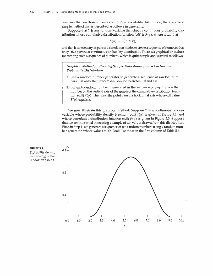
206 CHAPTER 5 Simulation Modeling: Concepts and Practice

FIGURE 5.2 Probability density function f(y) of the random variable Y.

numbers that are drawn from a continuous probability distribution, there is a very simple method that is described as follows in generality.

Suppose that Y is any random variable that obeys a continuous probability dis­tribution whose cumulative distribution function (cdf) is F(y), where recall that

F(y) = P(Y :5 y),

and that it is necessary as part of a simulation model to create a sequence of numbers that obeys this particular continuous probability distribution. There is a graphical procedure for creating such a sequence of numbers, which is quite simple and is stated as follows:

Graphical Method for Creating Sample Data drawn from a Continuous Probability Distrib11 tion

1. Use a random number generator to generate a sequence of random num­bers that obey the uniform distribution between 0.0 and 1.0.

2. For each random number x generated in the sequence of Step 1, place that number on the vertical axis of the graph of the cumulative distribution func­tion ( cdf) F (y). Then find the pointy on the horizontal axis whose cdf value F(y) equals x.

We now illustrate this graphical method. Suppose Y is a continuous random variable whose probability density function (pdf) f(y) is given in Figure 5.2, and whose cumulative distribution function (cdf) F(y) is given in Figure 5.3. Suppose that we are interested in creating a sample of ten values drawn from this distribution. First, in Step 1, we generate a sequence of ten random numbers using a random num­ber generator, whose values might look like those in the first column of Table 5.6.

f(y) 0.3

0.2

0.1

0'--~---'-~~--0C..~~..__~-'-~~_.__~~~~---'-~~-'-~--"--~~

0.0 1.0 2.0 3.0 4.0 5.0

y 6.0 7.0 8.0 9.0 10.0

FIGURE 5.3 Cumulative distribution function F(y) of the random variable Y.

TABLE 5.6 A sequence of ten random numbers.

5.6 Creating Numbers that Ob(•y ,t Co11111111011, Pro1>.,1>1l11y Di\lribution 207

F(y)

1.0

0.9

0.8

0.7

0.6

0.5

0.4

0.3

0.2

0.1

0.0 0.0 1.0 2.0

Random Number (x)

0.8054 0.6423 0.8849 0.6970 0.2485 0.0793 0.7002 0.1491 0.4067 0.1658

3.0 4.0

Value ofy

5.0

y

6.0 7.0 8.0 9.0 10.0

In order to create the sample value for the first random number, which is x = 0.8054, we place that value on the vertical axis of the cumulative distribution function F (y) of Figure 5.3 and determine the corresponding y value on the hori­zontal axis from the graph. This is illustrated in Figure 5.4. For x = 0.8054, the corre­sponding y value is (approximately) y = 6.75. Proceeding in this manner for all of the ten different random number values x, one obtains the ten values of y depicted in Table 5.7. These ten values of y then constitute a sample of observed values drawn from the probability distribution of Y.

As just shown, it is quite easy to perform the necessary steps of the graphical method. However, it may not be obvious why this method creates a sequence of val­ues of y that are in fact drawn from the probability distribution of Y. We now give some intuition as to why the method accomplishes this.

Consider the probability density function (pdf) f(y) of Y shown in Figure 5.2 and its associated cumulative distribution function (cdf) F(y) shown in Figure 5.3. Remember that the cdf F (y) is the area under the curve of the pdf f (y) . Therefore, the slope of F (y) will be steeper for those values of y where the pdf f (y) is higher, and

208 CHAPTER 5 Simulation Modeling: Concepts and Practice

FIGURE 5.4 Illustration of the graphical method for creating observed values of a continuous random variable with cumulative distribution function F(y).

TABLE 5.7 Values of x and y.

F(y)

1.0

0.9

0.8

0.7

0.6

0.5

0.4

0.3

0.2

0.1

0.0 0.0 1.0 2.0

Random Number (x)

0.8054 0.6423 0.8849 0.6970 0.2485 0.0793 0.7002 0.1491 0.4067 0.1658

3.0

Value ofy

6.75 6.04 7.16 6.24 4.51 3.58 6.28 4.02 5.15 4.12

4.0 5.0

y

F 6.0 7.0 8.0 9.0 10.0

the slope of F(y) will be flatter for those values of y where the pdf f(y) is lower. For example, at y = 5.5, f (y) is quite large, and the slope of F (y) is quite steep. Also, for example, at y = 3.0, f(y) is quite small, and the slope of F (y) is quite flat.

Now consider the application of the graphical method for creating values of y. Note that by way of the construction, the method will produce a greater concentra­tion of values of y where the slope of the cdf F (y) is steeper. Likewise, the method will produce a lesser concentration of values of y where the slope of the cdf F (y) is flatter. Therefore, using the observation in the paragraph above, the method will pro­duce a greater concentration of values of y where the pdf f(y) is higher and will pro­duce a lesser concentration of values of y where the pdf f(y) is lower. As it turns out, this correspondence is precise, and so indeed the method will produce values of y that are exactly in accord with the underlying probability distribution of Y.

Although the method is best illustrated by considering a graph of the cdf F (y), it is not necessary to have a literal graph of the cumulative distribution function in order to use the method. In fact, another way to state the method without the use of graphs is as follows:

TABLE 5.8

Worksheet for generating the price of codfish in Rockport.

5 .6 Creating Numbers that Obey a Continuous Probability Distribution 209

General Method for Creating Sample Data Drawn from a Continuous Probability Distribution

1. Use a random number generator to generate a sequence of random num­bers that obey the uniform distribution between 0.0 and 1.0.

2. For each random number x generated in the sequence of Step 1, compute that value of y whose cumulative distribution function value is equal to x. That is, given x, solve the equation:

F (y) = P ( Y :5 y) = x

to obtain the value y. Then assign y as the value created.

This more general form of the method is now illustrated on the Conley Fisheries problem, where the task at hand is to create a sequence of prices for codfish at the port in Rockport, one price for each of the 20 days under consideration, in such a way that the created prices are samples drawn from the probability distribution of the daily price of codfish in Rockport. Recall that the daily price of codfish in Rockport obeys a Normal distribution with meanµ, = $3.65/lb. and with a standard deviation a- = $0.20/lb.

The first step is to use a random number generator to generate 20 random num­bers. Suppose this has been done, and the 20 random numbers are as shown in the second column of Table 5.8.

The second step is then to compute that value of y for which the equation

F(y) = P(Y :5 y) = x

Price of Codfish in Rockport Day Random Number ($/lb.)

1 0.3236 3.5585 2 0.1355 3.4299 3 0.5192 3.6596 4 0.9726 4.0342 5 0.0565 3.3330 6 0.2070 3.4866 7 0.2481 3.5139 8 0.8017 3.8196 9 0.2644 3.5240

10 0.2851 3.5365 11 0.7192 3.7661 12 0.7246 3.7693 13 0.9921 4.1330 14 0.5227 3.6614 15 0.0553 3.3309 16 0.5915 3.6963 17 0.0893 3.3810 18 0.3136 3.5529 19 0.0701 3.3550 20 0.8309 3.8416

210 CHAPTER 5 Simulation Modeling: Concepts and Practice

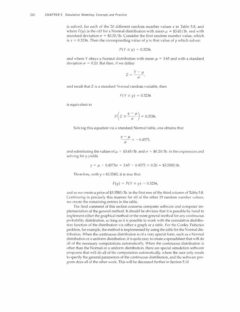
is solved, for each of the 20 different random number values x in Table 5.8, and where F(y) is the cdf for a Normal distribution with meanµ, = $3.65/lb . and with standard deviation CT = $0.20/lb. Consider the first random number value, which is x = 0.3236. Then the corresponding value of y is that value of y which solves:

P(Y s y) = 0.3236,

and where Y obeys a Normal distribution with meanµ, = 3.65 and with a standard deviation CT = 0.20. But then, if we define

z = Y- µ, CT I

and recall that Z is a standard Normal random variable, then

P(Y s y) = 0.3236

is equivalent to

( y - µ,)

P Z s -CT- = 0.3236.

Solving this equation via a standard Normal table, one obtains that

Y - J.L = -0.4575, CT

and substituting the values ofµ, = $3.65/lb. and <r = $0.20/lb. in this expression and solving for y yields

y = µ, - 0.4575CT = 3.65 - 0.4575 X 0.20 = $3.5585/ lb.

Therefore, with y = $3.5585, it is true that

F(y) = P(Y s y) = 0.3236,

,ind so we create a price of $3.5585/lb. in the first row of the third column of Table 5.8. Continuing in precisely this manner for all of the other 19 random number vcilucs, we create the remaining entries in the table.

The final comment of this section concerns computer softwme and computer im­plementation of the general method. It should be obvious that it is possible by hand to implement either the graphical method or the more general method for any continuous probability distribution, so long as it is possible to work with the cumulative distribu­tion function of the distribution via either a graph or a table. For the Conley Fisheries problem, for example, the method is implemented by using the table for the Normal dis­tribution. When the continuous distribution is of a very special form, such as a Normal distribution or a uniform distribution, it is quite easy to create a spreadsheet that will do all of the necessary computations automatically. When the continuous distribution is other than the Normal or a uniform distribution, there are special simulation software programs that will do all of the computation automatically , where the user only needs to specify the general parameters of the continuous distribution, and the software pro­gram does all of the other work. This will be discussed further in Section 5.10

5.7

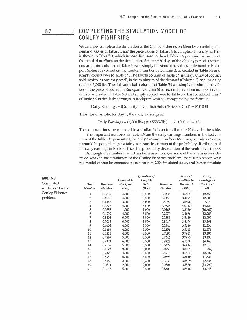
TABLE 5.9 Completed vVorksheetforthe Conle y Fisheries problem .

5.7 Completing the Simulation ModPI of Co11!Py Fisheries 211

COMPLETING THE SIMULATION MODEL OF CONLEY FISHERIES

We can now complete the simulation of the Conley Fisheries problem by combining lhl' demand values of Table 5.5 and the price values of Table 5.8 to complete the analysis. · 1 ·his is shown in Table 5.9, which is now discussed in detail. Table 5.9 portrays the results of the simulation efforts on the simulation of the first 20 days of the 200-day period. The SL'C­

ond and third columns of Table 5.9 are simply the simulated values of demand in Rock­port (column 3) based on the random number in Column 2, as created in Table 5.5 and simply copied over to Table 5.9. The fourth column of Table 5.9 is the quantity of codfish sold, which, as one may recall, is the minimum of the demand (Column 3) and the daily catch of 3,500 lbs. The fifth and sixth columns of Table 5.9 are simply the simulated val­ues of the price of codfish in Rockport (Column 6) based on the random number in Col­umn 5, as created in Table 5.8 and simply copied over to Table 5.9. Last of all, Column 7 of Table 5.9 is the daily earnings in Rockport, which is computed by the formula:

Daily Earnings = (Quantity of Codfish Sold) (Price of Cod) - $10,000.

Thus, for example, for day 1, the daily earnings is:

Daily Earnings= (3,500 lbs.) ($3.5585/lb.) - $10,000 = $2,455.

The computations are repeated in a similar fashion for all of the 20 days in the table. The important numbers in Table 5.9 are the daily earnings numbers in the last col­

umn of the table. By generating the daily earnings numbers for a large number of days, it should be possible to get a fairly accurate description of the probability distribution of the daily earnings in Rockport, i.e., the probability distribution of the random variable F.

Although the number n = 20 has been used to show some of the intermediary de­tailed work in the simulation of the Conley Fisheries problem, there is no reason why the model cannot be extended to run for n = 200 simulated days , and hence simulate

Quantity of Price of Daily Demand in Codfish Codfish in Earnings in

Day Random Rockport Sold Random Rockport Rockport Number Number (lbs.) (lbs.) Number ($/lb.) ($)

1 0.3352 4,000 3,500 0.3236 3.5585 $2,455 2 0.4015 4,000 3,500 0.1355 3.4299 $2,005 3 0.1446 3,000 3,000 0.5192 3.6596 $979 4 0.4323 4,000 3,500 0.9726 4.0342 $4,120 5 0.0358 1,000 1,000 0.0565 3.3330 ($6,667) 6 0.4999 4,000 3,500 0.2070 3.4866 $2,203 7 0.8808 6,000 3,500 0.2481 3.5139 $2,299 8 0.9013 6,000 3,500 0.8017 3.8196 $3,368 9 0.4602 4,000 3,500 0.2644 3.5240 $2,334

10 0.3489 4,000 3,500 0.2851 3.5365 $2,378 11 0.4212 4,000 3,500 0.7192 3.7661 $3,181 12 0.7267 5,000 3,500 0.7246 3.7693 $3,193 13 0.9421 6,000 3,500 0.9921 4.1330 $4,465 14 0.7059 5,000 3,500 0.5227 3.6614 $2,815 15 0.1024 3,000 3,000 0.0553 3.3309 ($7) 16 0.2478 4,000 3,500 0.5915 3.6963 $2,937 17 0.5940 5,000 3,500 0.0893 3.3810 $1,834 18 0.4459 4,000 3,500 0.3136 3.5529 $2,435 19 0.0511 2,000 2,000 0.0701 3.3550 ($3,290) 20 0.6618 5,000 3,500 0.8309 3.8416 $3,445

212 CHAPTER 5 Sirnuiation Modeling: Concepts and Practice

i1 = 200 days of dai ly earnings. Indeed, Table 5.10 shows 200 different daily earnings numbers generated by using the simulation methodology for 200 different days. Note that the first 20 entries in Table 5.10 are simply the daily earnings in Rockport of the first 20 days of the simulation , i.e., they are the numbers from the final column of Table 5.9.

TABLE 5.10 Daily Daily Daily Daily

Simulation output Eamings Eamings Earnings Earnings

in in in in for n = 200 Day Rockport J)c1y Rockport Day Rockport Day Rockport

simulation trials of Number ($) N11111/1cr ($) Number ($) Numbe1· ($)

the Conley Fisheries 1 $2,455 "I $2,870 101 $3,188 151 ($3,039)

model. 2 $2,005 ::;::: $2,530 102 $2,907 152 $1,822

3 $979 .r:;J $4,289 103 $4,192 153 $2,217 4 $4,120 ::;j $1,968 104 $2,792 154 $3,068 5 ($6,667) ."'"' ($2,382) 105 $2,727 155 ($224) 6 $2,203 Sr, $3,271 106 $1,930 156 $3,662 7 $2,299 :-i7 $2,457 107 $2,569 157 $3,829 8 $3,368 ,x $2,240 108 $2,858 158 $1,628 9 $2,334 r;q $2,658 109 $3,783 159 ($10,000)

10 $2,378 (1() $1,443 110 ($2,523) 160 $2,254 11 $3,181 hi ($6,491) 111 ($2,290) 161 $3,406 12 $3,193 h::'. $1,954 112 $4,229 162 $441 13 $4,465 h> ($6,284) 113 $3,317 163 ($3,159) 14 $2,815 (1..J. $2,494 114 ($1,769) 164 $3,243 15 ($7) (i::; $3,649 115 $2,581 165 $],351 ·16 $2,937 (i(i $3,258 116 $2,361 166 $3,649 17 $1,834 <i7 ($2,034) 117 ($10,000) 167 $3,156 18 $2,435 68 $2,791 118 $919 ·168 $2,104 Ill ($3,290) ()l) $2,856 119 $2,493 169 $2,573 20 $3,445 70 $2,026 120 $.1,LJ73 170 $2,0II 21 $2,076 71 $2,677 121 $3 , 18LJ 171 $3,706 22 $3,583 72 $3,364 122 ($3 ,654) 172 $2,017 23 $2,169 73 $3,472 123 $2,4LJ2 173 ($2,860) 24 $3,064 74 $1,873 124 $2,84J 174 $2,247 2:i ($6,284) 75 $2,104 125 ($3,ll20) 175 $2,lhS 2(, $3,602 76 $2,586 ·126 $2 ,725 ·17r, $4,134 27 $4,406 77 $2,201 127 $2 , 194 177 $3,011 28 $2,911 78 $1,82:'i 128 $1,883 ]78 $2,34:'i 2LJ $2,389 79 $2,955 129 $3 ,329 179 $1,41b

30 $2,752 80 $1,469 130 $2,372 ]80 $3 ,025 31 $2,163 81 $1,843 131 $1,010 18] $15<,

32 $3,553 82 $3,936 l32 $3,161 182 $2,737 :n $3,315 83 $2,572 i:n $2,769 ]83 $3,025 J4 $1,936 84 ($Hl,OOO) 134 $3,184 184 ($3 ,328

35 $3,013 85 $-1,60! 135 $2,786 185 $2,163 1h $405 86 $4,2J8 l36 $3,233 186 ($2,1in)

J7 $2,443 87 $2,423 137 $2,230 187 $1,1141

18 $2,825 88 $1,072 138 $3,338 188 $2,110

39 $1,818 89 $2,651 139 $2,670 189 $2,980 40 ($1,808) 90 $-1,821 140 ($6,%2) ·190 $J ,-109

41 $3,104 91 $2,782 141 $2,50ll llJI $3,24h -1-2 $2,802 92 ($5,%3) 142 ($3,068) ·192 $2 ,567 41 $556 93 $2,904 143 $2,(l:16 193 $3 ,34()

4-1- $2,554 94 $J ,tJ72 144 $-UlJll 194 $2,2-1--1-45 $2,792 95 $2,539 145 $3 ,826 ]95 $3,219 -l-6 $3,099 96 $1,530 146 $1 ,527 196 $2,4%

-1-7 $2,465 97 $l,b29 147 $3,1% 197 $2,(Jll

48 $2,909 LJ8 $2,610 148 $J,573 198 $2,731 ..j.l) $2,386 99 $2,821 149 $4,020 199 ($6,46--1-)

50 $2,505 10(] $2,067 150 $3 ,012 I 200 $3,61-l-

5.8 Using the Sample Data for Analysis 213

_s_.s __ __.., I USING THE SAMPLE DATA FOR ANALYSIS

Table 5.10 contains a sample of n = 200 observed values of the earnings from using Rockport. Fixing some notation, let xi denote the daily earnings from using Rockport for day number i, for all values of i = 1, ... , 200. That is, x 1 = $2,455, x2 = $2,005, ... , x200 = $3,614. Then each xi is the observed value of the random vari­able F and has been drawn from the (unknown) probability distribution of the random variable F. In fact, the array of values x1, x2, ..• , x200 constitutes a fairly large sample of n = 200 different observed values of the random variable F. Therefore, we can use this sample of observed values to estimate the answers to the five questions posed in Section 5.1 and Section 5.2, which we rephrase below in the language of statistical sampling:

(a) What is the shape of the probability density function of F?

(b) What is P(F > $1,375)?

(c) What is P(F < $0)?

( d) What is the expected value of F?

(e) What is the standard deviation of F?

We now proceed to answer these five questions.

Question (a):

What is an estimate of the shape the probability density function of F? Recall from Chapter 4 that in order to gain intuition about the shape of the distrib­

ution of F, it is useful to create a frequency table and a histogram of the observed sam­ple values x1, x2, ..• , x200 of Table 5.10. Such a frequency table is presented in Table 5.11.

A histogram of the values of Table 5.11 is shown in Figure 5.5. This histogram gives a nice pictorial view of the distribution of the observed values of the sample, and it also is an approximation of the shape of the probability density function (pdf) of F. We see from the histogram in Figure 5.5 that the values of F are mostly clustered in the range $0 through $4,500, in a roughly bell shape or Normal shape, but that there are also a signifi­cant number of other values scattered below $0, whose values can be as low as -$10,000. This histogram indicates that while most observed values of earnings from Rockport are quite high, there is some definite risk of substantial losses from using Rockport.

Question (b):

What is an estimate of P(F > $1,375)? This question can be answered by using the counting method developed in

Chapter 4. Recall from Chapter 4 that the fraction of values of x1, x2, .•• , x200 in Table 5.10 that are larger than $1,375 is an estimate of the probability p for which

p = P(F > $1,375).

If we count the number of values of X1, x2, ... , x200 in Table 5.10 that are larger than $1,375, we obtain that 165 of these 200 values are larger than $1,375. Therefore, an es­timate of p = P(F > $1,375) is:

165 200 = 0.83.

We therefore estimate that there is an 83% likelihood that the earnings in Rockport on any given day would exceed the earnings from Gloucester. This supports the strategy option of choosing Rockport over Gloucester.

214 CHAPTER 5

TABLE 5.11 Frequency table of the 200 observed values of earnings in Rockport.

FIGURE 5.5

His togram of L'cHnings from Rockport.

Simulation Modeling: Concepts and Practice

Interval From Interval To Number in the Sample

($10,500) ($10,000) 3 ($10,000) ($9,500) 0

($9,500) ($9,000) 0 ($9,000) ($8,500) 0 ($8,500) ($8,000) 0 ($8,000) ($7,500) 0 ($7,500) ($7,000) 0 ($7,000) ($6,5ll0) 1 ($6,500) ($6,0llO) 5 ($6,000) ($5,500) 1 ($5,500) ($5,llll()) 0 ($5,000) ($4,5()()) 0 ($4,500) ($4,0llll) 0 ($4,000) ($1/i()()) 1 ($3,500) ($1,lHHl) 5 ($3,000) ($2,5()()) 2 ($2,500) ($2,!Hlll) 4 ($2,000) ($1,500) 2 ($1,500) ($1,(llll)) 0 ($1,000) ($500) 0

($500) $0 2 $0 $500 3

$500 $1,000 3 $1,000 $1,500 6 $1,500 $2,000 17 $2,000 $2,500 43 $2,500 $3,000 41 $3,000 $3,500 35 $3,500 $4,000 16 $4,000 $4,500 10 $4,500 $5,000 ()

50

45

40

35

;..., 10 u c: 'lJ

25 :::; r:;;' 'lJ

J:: 20

15

]()

5

() I; ' e] ij Q

-$·10,000 -$8,000 -$6,000 -$4,000 -$2,()()() $() $2,000 $-t,000

Earning s from R\lckport-

5.8 Using the Sample Data for Analysis 215

Question (c):

What is an estimate of P(F < O)? This question can also be answered by using the counting method of Chapter 4.

Recall from Chapter 4 that the fraction of values of Xi, x2, .•• , x200 in Table 5.10 that are less than $0 is an estimate of the probability p for which p = P ( F < $0). If we count the number of values of Xi, x2, ••• , x200 in Table 5.10 that are less than $0, we obtain that 26 of these 200 values are less than $0. Therefore, an estimate of p = P(F < $0)is:

26 200 = 0.13.

We therefore estimate that there is a 13%likelihood that Conley Fisheries would lose money on any given day, if they chose to sell their catch in Rockport. This shows that the risk of choosing Rockport is not too large, but it is not insubstantial either.

Question (d):

What is an estimate of the expected value of F? We know that the observed sample mean x of this sample of 200 observed values

is a good estimate of the actual expected value µ of the underlying distribution of F, especially when the sample size is large (and here, the sample size is n = 200, which is quite large). Therefore, the observed sample mean of the 200 values Xi, x2, ••• , x200

in Table 5.10 should be a very good estimate of the expected valueµ, of the random variable F. It is straightforward to obtain the sample mean x for the sample given in Table 5.10. Its value is

_ = 2,445 + 2,005 + ... +3,614 = $17 8 38 X

200 I 6 • •

Therefore our estimate of the mean of the random variable Fis $1,768.38. Notice that this value is larger than $1,375, which is the earnings that Conley Fisheries can obtain (with certainty) by selling its fish in Gloucester. Thus, an estimate of the expected in­crease in revenues from selling in Rockport is

$393.38/ day = $1,768.38/ day - $1,375.00/ day.

Question (e): What is an estimate of the standard deviation of F?

Recall from the statistical sampling methodology of Chapter 4 that the observed sample standard deviations is a good estimate of the actual standard deviation u of the random variable F, especially when the sample size is large. It is straightforward to obtain the observed sample standard deviation for the sample given in Table 5.10, as follows:

11

L (x; - x)2 s2 = _i =_1 ___ _

n - 1

(2,455 - 1,768.38)2 + (2,005 - 1,768.38)2 + ... + (3,614 - 1,768.38)2

200 - 1

= 7,142,715.87.

Therefore

216 CHAPTER 5 Simulation Modeling: Concepts and Practice

s = V7,142,715.s7 = $2,672.59,

and our estimate of the standard deviation of Fis s = $2,672.59. This standard devi­ation is rather large, which confirms Clint Conley's intuition that there is substantial risk involved in using Rockport as the port at which to sell his daily catch.

An additional question that one might want to answer is: What is a 95% confi­dence interval for the mean of the distribution of daily earnings from selling the catch of codfish in Rockport? The answer to this question is provided by the formula in Chapter 4 for a 95% confidence interval for the mean of a distribution when n is large. This formula is:

[x - l.96s/ Vn, x + l.96s/ Vn].

Substituting the values of x = $1,768.38, s = $2,672.59, and n = 200, we compute the 95% confidence interval for the true mean of the distribution of daily earnings to be

[$1,397.98, $2,138.78].

Notice that this interv,11 does not contain the value $1,375. Therefore, at the 95% confidence level, we can conclude that the expected daily earnings from selling the catch of codfish in Rockport is higher than from selling the catch of codfish in Gloucester.

Finally, suppose Clint Conley were to construct and use the simulation model that has been developed herein . With the answers to the questions posed earlier, he would be in a good position to make an informed decision . Here is a list of the key data garnered from the analysis of the simulation model:

• We estimate that the shape of the distribution of daily earnings from Rockport will be as shown in Figure 5.5. On most days the earnings will be between $0 and $4,500 per day. However, on some days this number could be as low as -$10,000.

• We estimate that the probability is 0.83 that the daily earnings in Rockport would be greater than in Gloucester on any given day.

• We estimate that the probability is 0.13 that the daily earnings in Rockport will be negative on any given day.

• We estimate that the expected daily earnings from Rockport is $1,768.38. This is higher than the earnings in Gloucester would be, by $393.38/day .

• We estimate that the standard deviation of the daily earnings in Rockport is $2,672.59.

• The 95% confidence interval for the actual expected daily earnings from using Rockport excludes $1,375. Therefore, we are 95% confident that the expected daily emnings from Rockport is higher than from Gloucester.

Based on this information, Clint Conley would probably optimally choose to sell his catch in Rockport, in spite of the risk. Note that the risk is not trivial, as there is always the possibility that he could lose money on any given day (with probability 0.13), and in fact he could have cash-flow problems if he were extremely unlucky. But unless he is extremely averse to taking risks (in which case he might not want to be in the fishing industry to begin with), he would probably further the long-term in­terests of Conley Fisheries by choosing to sell his fish in Rockport.

5.9

5.10

5.10 Computer Software for Simulation Modeling 217

SUMMARY OF SIMULATION MODELING,AND GUIDELINES ON THE USE OF SIMULATION

A simulation model attempts to measure aspects of uncertainty that simple formulas cannot. As we saw in the Conley Fisheries problem, even this simple problem has no convenient analysis via formulas related to probability and random variables. Of course, when formulas and tables can be used instead of a simulation model, then the manager's task is that much easier. But all too often, there are situations that must be analyzed where a simulation model is the only appropriate methodological tool.

The successful application of a simulation model depends on the ability to cre­ate sample values of random variables that obey a variety of discrete and continuous probability distributions. This is the key to constructing and using a simulation model. Through the use of a random number generator, it is possible to create sam­ple data values that obey any discrete distribution or any continuous distribution by applying the general methods outlined in Section 5.5 (for discrete random variables) and Section 5.6 (for continuous random variables).

Unlike decision trees and certain other modeling tools, a simulation has no in­ternal optimal decision-making capability. Note that the simulation model con­structed for analyzing the Conley Fisheries problem only produced data as the output, and the model itself did not choose the best port strategy. Suppose that Con­ley Fisheries faced the decision of choosing among five different ports. A simulation model would be able to analyze the implications of using each port, but unlike a de­cision tree model, the simulation model would not choose the optimal port strategy. In order to use a simulation model, the manager must enumerate all possible strat­egy options and then direct the simulation model to analyze each and every option.

The results that one can obtain from using a simulation model are not precise due to the inherent randomness in a simulation. The typical conclusions that one can draw from a simulation model are estimates of the shapes of distributions of partic­ular quantities of interest, estimates of probabilities of events of interest, and means and standard deviations of the probability distributions of interest. One can also con­struct confidence intervals and other inferences of statistical sampling .

The question of the number of trials or runs to perform in a simulation model is mathematically complex. Fortunately, with today's computing power, this is not a paramount issue for most problems, because it is possible to run even very large and complex simulation models for many hundreds or thousands of trials, and so obtain a very large set of sample data values to work with.

Finally, one should recognize that gaining managerial confidence in a simulation model will depend on at least three factors:

• a good understanding of the underlying management problem,

• one's ability to use the concepts of probability and statistics correctly, and

• one's ability to communicate these concepts effectively.

COMPUTER SOFTWARE FOR SIMULATION MODELING

The Conley Fisheries example illustrates how easy it is to construct a simulation model using standard spreadsheet software. The "input" to the Conley Fisheries ex­ample consisted of the following information:

218 CHAPTER 5 Simulation Modeling: Concepts and Practice

5.11

• the description of probability distribution of the random variable D, the daily de­mand in Rockport. This distribution was shown in Table 5.1.

• the description of the probability distribution of the random variable PR, the daily price of codfish in Rockport. This is a Normal distribution with mean µ, = $3.65 and standard deviation a = $0.20.

• the formula for the earnings from selling the catch in Rockport, namely

F = PR x min(3,500, D) - 10,000.

Based on these inputs , we constructed a simulation model predicated on the ability to generate random variables that obey certain distributions, namely a discrete distrib­ution (for daily demand in Rockport) and the Normal distribution (for daily prices in Rockport). The output of the model was the sample of observed values of earnings in Rockport shown in Table 5.10. Based on the information in Table 5.10, we constructed a histogram of the sample observations (shown in Figure 5.5), and we performed a va­riety of other computations, such as counting the number of observations in a given range, the computation of the sample mean and the sample standard deviation, etc.

Because simulation modeling is such a useful tool, there are a variety of simula­tion modeling software products that facilitate the construction of a simulation model. A typical simulation software package is usually designed to be used as an add-on to the ExcelQ9 spreadsheet software and has pull-down menus that allows the user to choose from a variety of probability distributions for the generation of random variables (such as the uniform distribution, the Normal distribution, the bi­nomial distribution, a discrete distribution, etc.) The software is designed to auto­matically generate random numbers that obey these distributions. Furthermore, the typical simulation software package will automatically perform the routine tasks in­volved in analyzing the output of a simulation model, such as creating histograms, estimating probabilities, and estimating means and standard deviations. All of this capability is designed to free the manager to focus on managerial analysis of the sim­ulation model, as opposed to generating random numbers and creating chart output. An example of such a software package that is used in some of the case s in Section 5.12 is called CrystalBall ® and is described at 'the end of the Ontario Gateway case.

There are also a large number of "specialty simulation" software packages that are designed for specific uses in specific applications domains. For example, there are some simulation modeling software packages designed to model manufacturing op­erations, and that offer special graphics and other features unique to a manufactur­ing environment. There are other simulation modeling software packages designed for other special application domains, such as service applications, military applica­tions, and financial modeling.

TYPICAL USES OF SIMULATION MODELS

Perhaps the most frequent use of simulation models is in the analysis of a company's production operations. Many companies use simulation to model the events that oc­cur in their factory production processes, where the times that various jobs take is un­certain and where there are complex interactions in the scheduling of tasks. These models are used to evaluate new operations strategies, to test the implications of us­ing new processes, and to evaluate various investment possibilities that are intended to impro ve production and operational efficiency.

5.12

5.12 Case Modules 219

Another frequent use of simulation models is in the analysis of operations where there are likely to be queues (that is, waiting lines). For example, the best managed fast-food chains use simulation models to analyze the effects of different staffing strategies on how long customers will wait for service, and on the implications of of­fering new products, etc. Banks use simulation models to assess how many tellers or how many ATMs (automated teller machines) to plan for at a given location. Airlines use simulation modeling to analyze throughput of passengers at ticket counters, at gates, and in baggage handling. With the increasing use of toll-free numbers for serv­ing customers in a variety of businesses (from catalog shopphlg to toll-free software support for software products), many telecommunications companies now offer sim­ulation modeling as part of their basic service to all of their "800" business customers to help them assign staffing levels for their toll-free services.

Another use of simulation modeling is in capital budgeting and the strategic analysis of investment alternatives. Simulation models are used to analyze the im­plications of various assumptions concerning the distribution of costs of an invest­ment, possible market penetration scenarios, and the distribution of cash-flows, both in any given year as well as over the life of the investment.

As mentioned earlier, simulation models are used quite abundantly in the analy­sis of military procurement and in the analysis of military strategy. Here in particu­lar, simulation modeling is used to great advantage, as the alternative of testing new hardware or tactics in the field is not particularly attractive.

Simulation is also used in financial engineering to assign prices and analyze other quantities of interest for complex financial instruments, such as derivative se­curities, options, and futures contracts.

This is only a small list of the ways that simulation models are currently used by managers. With the rapid advances in both computer hardware and the ease of use of today's simulation modeling software, there is enormous potential for simulation models to add even more value to the educated and creative manager who knows how to wisely use the tools of simulation.

CASE MODULES

THE GENTLE LENTIL RESTAURANT

An Excel lent Job Offer

Sanjay Thomas, a second-year MBA student at the M.I.T. Sloan School of Manage­ment, is in a very enviable position: He has just received an excellent job offer with a top-flight management consulting firm. Furthermore, the firm was so impressed with Sanjay's performance during the previous summer that they would like Sanjay to start up the firm's practice in its new Bombay office. The synergy of Sanjay's pre­vious consulting experiences (both prior to Sloan and during the previous summer), his Sloan MBA education, and his fluency in Hindi offer an extremely high likelihood that Sanjay would be very successful, if he were to accept the firm's offer and de­velop the Bombay office's practice in India and southern Asia.