simulation of advanced microfluidic systems with ... · simulation of advanced microfluidic...
TRANSCRIPT

RESEARCH PAPER
Simulation of advanced microfluidic systems with dissipativeparticle dynamics
Thomas Steiner Æ Claudio Cupelli Æ Roland Zengerle ÆMark Santer
Received: 8 October 2008 / Accepted: 11 November 2008 / Published online: 9 January 2009
� Springer-Verlag 2008
Abstract Computational Fluid Dynamics (CFD) is
widely and successfully used in standard design processes
for microfluidic lTAS devices. But for an increasing
number of advanced applications involving the dynamics
of small groups of beads, blood cells or biopolymers in
microcapillaries or sorting devices, novel simulation tech-
niques are called for. Representing moving rigid or flexible
extended dispersed objects poses serious difficulties for
traditional CFD schemes. Meshless, particle-based simu-
lation approaches, such as Dissipative Particle Dynamics
(DPD) are suited for addressing these complicated flow
problems with sufficient numerical efficiency. Objects can
conveniently be represented as compound objects embed-
ded seamlessly within an explicit model for the solvent.
However, the application of DPD and related methods to
realistic problems, in particular the design of microfluidics
systems, is not well developed in general. With this work,
we demonstrate how the method appears when used in
practice, in the process of designing and simulating a
specific microfluidic device, a microfluidic chamber
representing a prototypical bead-based immunoassay
developed in our laboratory (Glatzel et al. 2006a, b;
Riegger et al. 2006).
Keywords Dissipative particle dynamics �Simulation of microfluidic systems � Lab on a chip
1 Introduction
One of the main objectives of life science, a discipline
comprising fields as diverse as environmental technology,
biochemistry, pharmacology and medical diagnostics, is an
attempt to transfer fundamental research results to com-
mercial applications and products. One of the fastest
growing fields in this area is the development of so called
Lab-On-A-Chip devices, or with special emphasis on
diagnostics applications, Micro-Total-Analysis Systems
(lTAS) (Vilkner et al. 2004; Oosterbroek and van den Berg
2003; Haeberle and Zengerle 2007; Harrison et al. 2000;
Ducree and Zengerle 2004; Reyes et al. 2002; Auroux
et al. 2002). Their virtues are miniaturization and integra-
tion of several chemical or biochemical analysis steps with
various microfluidic tasks to process or transport reagents.
In medical diagnostics, several lTAS have been developed
so far, e.g., to enhance the screening of cardiovascular
drugs (Li et al. 2003), to simultaneous detect cardiac risk
factors (Kurita et al. 2006; Christodoulides et al. 2002) or
to monitor in vivo the glucose and lactate concentration
(Kurita et al. 2002, 2006) as well as a wide variety of
immunoassays (Sato and Kitamori 2004; Yakovleva et al.
2002, 2003a, b). In a way similar to applying finite-element
or electronic-circuit simulation tools for the design of
MEMS, CFD-simulations have become an indispensable
tool in the development process of these microfluidic
devices. They guarantee reliable designs and help reduce
costs during the development phase.
lTAS may involve quite complex mixtures of biological
liquids such as emulsions (Haeberle et al. 2007; Hardt and
Thomas Steiner: born Glatzel.
T. Steiner � C. Cupelli � R. Zengerle � M. Santer
Department of Microsystems Engineering IMTEK,
University of Freiburg, Georges-Kohler-Allee 106,
79110 Freiburg, Germany
M. Santer (&)
Fraunhofer Institute for Mechanics of Materials-IWM,
Wohlerstrasse 9, 79108 Freiburg, Germany
e-mail: [email protected]
123
Microfluid Nanofluid (2009) 7:307–323
DOI 10.1007/s10404-008-0375-4

Schonfeld 2003; Hessel et al. 2003) and cell suspensions
(MacDonald et al. 2003; Tabuchi et al. 2004), in combi-
nation with added objects such as functionalized colloids or
microbeads (Sugiura et al. 2005; Lettieri et al. 2003; Kerby
et al. 2002; Sohn et al. 2005). With an increasing number
of devices one attempts to manipulate these complex fluids
in a controlled manner—examples are bead-based micro-
mixers and immunoassays (Riegger et al. 2006; Grumann
et al. 2005; Sato et al. 2002; Saleh and Sohn 2003; Roos
and Skinner 2003), cell sorting or DNA-separation devices
(Yoshida et al. 2003; Wolff et al. 2003; Dittrich and
Schwille 2003; Tian et al. 2000; Tian and Landers 2002;
Sanders et al. 2003; Doyle et al. 2002; Duong et al. 2003).
In these systems, one is dealing with rather complex situ-
ations of fluid flow. On the one hand, the number and shape
of dispersed objects is so large that their extent and mutual
interaction cannot be neglected. On the other hand, they are
too few to be described effectively as a rheological fluid
with properties that can be parametrized. Additionally, as
in the case of emulsions or blood cells, the elastic flexi-
bility of an object has to be taken into account. Because of
the great difficulties in generating adaptive and time-
dependent meshes, it is impractical for finite-volume
schemes to deal with this situation in great generality.
During the last 15 years, various new meshless and
particle-based simulation approaches have received con-
siderable attention that can offer solutions to the above-
mentioned flow problems (Heyes et al. 2004). Among them
are, most notably, recent developments in Smoothed Par-
ticle Hydrodynamics (SPH) (Monaghan 1992), Lattice gas
methods (LGM) (Frisch et al. 1986) and Dissipative Par-
ticle Dynamics (DPD). LGM such as the Lattice-
Boltzmann-Method implement a pseudo-molecular colli-
sion dynamics on a grid in order to emulate the dynamical
properties of the Boltzmann equation. Thus, this elegant
scheme becomes a very powerful solver for fluid dynamics
problems, including even turbulence. Phenomena such as
multi-phase flows (Sbragaglia et al. 2007) have been
implemented, and studies addressing complete microfluidic
systems have recently been presented (Dupin et al. 2006).
The particle-based schemes that employ the solution
of Newton’s equation of motion to represent the system
dynamics seems conceptually simpler. SPH, for instance, is
actually an alternative discretization of the Navier–Stokes-
Equations (NSE), where the grid points represent fluid
elements that are co-moving with the local flow field in a
Lagrangian frame (Monaghan 2005). With each point, a
smooth kernel function is associated. The superposition of
kernels permits the evaluation of densities, velocities and
their derivatives at other points. The kernel functions lead
to effective forces between neighboring points—the initial
configuration of points can undergo a substantial redistri-
bution in space, establishing the picture of small interacting
amounts of liquid. In advanced schemes such as Smoothed-
Dissipative-Particle Dynamics (SDPD) the analogy with a
small thermodynamic system can be established by incor-
porating thermal fluctuations (Espanol and Revenga 2003).
DPD, in contrast, was originally proposed in a purely
heuristic manner (Hoogerbrugge and Koelman 1992), as an
explicit model for solvents and liquid flow on mesoscopic
scales. The novel idea was to combine soft repelling forces
of generic pseudo-molecules (supposed to represent lumps
of fluid) with a momentum-conserving thermostat to retain
hydrodynamics, while at the same time providing thermal
motion. This method was soon put on firm grounds and
improved by various authors (Lowe 1999; Masters and
Warren 1999; Trofimov 2003; Espanol and Warren 1995),
and must properly be viewed as providing a generic model
liquid. Technically, the scheme is quite similar to molec-
ular dynamics (MD) simulations—all properties of the
model liquid are completely specified by the given inter-
particle interactions, which usually are kept advantageous
numerically—the integration time step in DPD can be
chosen at least two orders of magnitude larger than in MD
(Groot and Warren 1997).
In the same spirit, one also may build structured objects
out of dissipative particles directly. The dynamics of single
polymer coils or polymer mixtures can be represented quite
faithfully by establishing linear or branched chains of
particles that are linked by harmonic forces (Groot and
Madden 1998). Solid boundaries or dispersed solid objects
may be defined by ‘‘freezing’’ the absolute or relative
motion of the constituting particles. This conceptual sim-
plicity renders the method very attractive for addressing
general problems in fluid dynamics that are hard to repre-
sent or simulate otherwise, irrespective of a particular
length or time scale. The rheology of suspensions of rigid,
arbitrarily-shaped objects has been studied quite success-
fully (Koelman and Hoogerbrugge 1993; Boek et al. 1997;
Pryamitsyn and Ganesan 2005), but also purely hydrody-
namic problems have been addressed—in studying flow
around periodic arrays of cylinders the DPD simulation
was shown to resolve even fine details of asymptotic cor-
rections to the flow field (Keaveny et al. 2005).
On the other hand, the majority of previous studies with
DPD and related methods have mostly been applied in
idealized situations in a rather generic manner. Many
aspects important for carrying out studies for specific
microfluidic systems are not yet well developed. In this
work, we explore the DPD approach with respect to rep-
resenting a realistic engineering problem involving the
design process of a special type of a microfluidic chamber
serving as a bead-based immunoassay. In this chamber,
microspheres with immobilized capture proteins are sup-
posed to aggregate in as regular a pattern as possible to
facilitate fluorescent readout (Riegger et al. 2006), see also
308 Microfluid Nanofluid (2009) 7:307–323
123

Fig. 1. Prerequisites for a regular and reproducible aggre-
gation pattern are a careful design of flow geometry, the
shape of the chamber and the interactions of the micro-
spheres (Roos and Skinner 2003; Stone et al. 2004). On the
way to a time-dependent simulation of the aggregation
process in comparison to experiments, we illustrate a
possible validation process, which will indeed reveal the
limitations but especially the virtues of the simulation
approach.
This work is organized as follows. In the following
section, we outline the fundamentals of the DPD approach.
Subsequently we discuss the role a DPD simulation can
play in a design process of a lTAS application. In some
detail, we explain the quaternion approach to representing
compound rigid objects, since it is a very efficient and
elegant method to propagate objects of arbitrary shape, but
does not appear to be widely used. Finally, we compare the
process of successive aggregation of microspheres to
experimental results.
2 Fundamentals of dissipative particle dynamics
In DPD, fluids and soft matter are modeled by pairwise
interacting particles [which we shall in general refer to as
fluid particles (FP)], the dynamics of which follows
Newton’s second law
Fi ¼ mi€ri; ð1Þ
with the mass mi of particle i and its spatial coordinate ri in
the laboratory-fixed frame. Fi is the total force acting on it.
In the simplest form, Fi is the sum of pairwise
conservative, dissipative and random forces,
Fi ¼X
j
FCij þ FD
ij þ FRij
� �þ Fext
i ; ð2Þ
Fexti is an external force such as gravity. The conservative
force in standard DPD is a soft central repulsion acting
between particle i and j:
FCij ¼
AijwCðrijÞeij rij\1
0 rij� 1;
�ð3Þ
where rij = ri-rj, rij = |rij| and eij = rij/rij. The weight
function wC(r) = (1-r/rc) vanishes for an inter-particle
distance r larger than a cutoff radius rc (cf Fig. 2a), and
determines the effective range of forces. rc is conveniently
taken as the unit of length, and is usually set to unity
(rc = 1). A soft potential allows to choose a large time step
in general, but would give rise to a very low viscosity. In
fact, if the conservative force is sufficiently weak, the
major part of the viscosity is provided by the dissipative
force FijD (Groot and Warren 1997),
FDij ¼
�cxDðrijÞðvij � eijÞeij rij\1
0 rij� 1;
�ð4Þ
with contributions from the random force FijR (Marsh et al.
1997),
FRij ¼
rwRðrijÞnijrijðDtÞ12 rij\1
0 rij� 1;
�ð5Þ
where r is the amplitude of the random variable nij. The
dissipative force is proportional to the relative velocity
vij = vi-vj of two FPs, as illustrated in Fig. 2b). Note the
dependence of FR on the square root of the integration time
step Dt: FijD and Fij
R obey a fluctuation–dissipation theorem
where r and c are related by r2 = 2ckBT and wijR(r)2 =
wijD(r), kB is the Boltzmann constant. Together they act as a
thermostat keeping the system at a defined temperature T.
a)
b)
Fig. 1 Typical read-out procedure for multiplexed bead-based
immunoassays as studied previously by the authors (Riegger et al.
2006). a First, the tagged beads are optically identified by their color.
b Second, the fluorescent intensity is measured for each optical tag
(color online)
a) b)
Fig. 2 a Pair-force of a fluid particle. b Calculation of the relative
velocity vij between two particles
Microfluid Nanofluid (2009) 7:307–323 309
123

The usual choice for the weight functions is wR = wC
(Espanol and Warren 1995). In this work, Eq. 1 is solved
with a Velocity-Verlet algorithm put forward by Groot and
Warren (1997) and described in Appendix B.1. Improved
versions of the thermostat (Lowe 1999; Peters 2004) have
been suggested to eliminate time step effects of the simple
Velocity-Verlet scheme (Vattulainen et al. 2002).
The forces introduced above are central, and imply
conservation of linear and angular momentum. Espanol
(1995) finally showed that if sufficient spatio-temporal
averages of velocities �v and densities �q are considered, the
NSE are obeyed with a well defined viscosity �g;
�qo
ot�vþ �q�v � r�v ¼ �rpþ �gr2�vþ �qg; ð6Þ
p is the pressure distribution and g, a body force. For the
simple force law (3) the equation of state (EOS) reads
p ¼ �qkBT þ aA�q2; ð7Þ
where a is a correction factor arising from a mean-field
approximation (Groot and Warren 1997). Many extensions
of the simple scheme above have been proposed, such as
additional internal degrees of freedom (Espanol 1998), or
tailor-made equations of state, including cohesive proper-
ties (Pagonabarraga and Frenkel 2001); Eq. 7 does not yet
provide a Van-der-Waals loop that would allow for the
coexistence of a vapor and a liquid phase.
Two comments are in order. First, with a chosen set of
model quantities (e.g., A, T and c) there is, in general, no
simple relation to transport parameters such as diffusivities
and viscosities; these must, strictly speaking, be deter-
mined by methods of statistical mechanics (Ripoll et al.
2001). In practice, however, this is rarely necessary, as
these properties are easily measured numerically for suf-
ficiently many reference points in parameter space by
standard methods of non-equilibrium MD (Allen and Til-
desley 1987). In our work, we have used Lees-Edwards
boundary conditions in order to obtain the viscosity mea-
sured at a spatially homogeneous shear rate. For vanishing
A, our results agree with the simple analytical estimate put
forward in Groot and Warren (1997). However, increasing
the interparticle repulsion to A = 250 (at r = 5, kBT = 1
and q = 5 will increase �g by roughly a factor of 6). Sec-
ond, as long as generic force laws are used, the EOS of the
model liquid will differ significantly from that of real
liquid. Thus, there is no immediate relation to a particular
time or length scale. Although a restricted mapping of
scales is possible for genuine nanoscale applications,
exploiting the stochastic character (Groot and Rabone
2001), for a general flow problem this would be rather
inconvenient. For instance, representing the relatively high
compressibility of a liquid on the scale of the simulation
box would require fairly strong repelling forces; but
increasing FC indefinitely not only increases the viscosity
(and thus the integration time step), but ultimately can
cause the model liquid to freeze (Trofimov 2003).
In practice, one would instead allow for a rather low
compressibility and check that the maximum Mach number
is sufficiently small. In fact, employing a set of relevant
dimensionless quantities to relate the simulation to the real
problem on the one hand, and characterizing the limits of
the model by another suitable set is the most natural (and
useful) way to proceed, as will be outlined in the following
section.
3 From design to simulation
3.1 Scope of the DPD modeling
Figure 3 illustrates the overall design of the aggregation
chamber. Beads enter the aggregation chamber successively
via a thin connecting channel preventing arrival in lumps
which could lead to badly-shaped aggregates. The figure
also indicates how a rapid-prototyping process for structure
optimization would eventually be organized—the CAD-
design of the structure serves for constructing both, a dis-
cretization mesh as input to a CFD-simulation and for
defining the location of immobile fluid particles constituting
a)
b)
c)
d)
e)
Fig. 3 Workflow from construction to simulation and fabrication
of lTAS devices. a CAD-Design, turned upside-down (the wall where
beads can aggregate (d) is shown to the top for better visibility). From
the CAD-data, a mesh of grid points can be generated (b) that serves
both, as discretization for a CFD-simulation (c) and (with an adapted
distribution of grid points) as the positions for solid fluid particles in
the DPD simulation (e) (color online)
310 Microfluid Nanofluid (2009) 7:307–323
123

the solid boundaries in the DPD-simulation (employing an
XYZ-format of the CAD-file). In a preliminary design cycle
(A), CFD-simulations would be used to quickly assess and
optimize the overall flow properties of the device, possibly
including the connecting peripheral fluidic components. In a
subsequent cycle (B), a detailed analysis including the
explicit dynamics of several aggregating microspheres is
left to the DPD simulation, which must then be restricted to
the reduced structure actually shown in the figure.
Naturally the question arises, whether the DPD scheme
and CFD may be coupled directly, e.g., by matching
stresses and mass flows across suitably chosen interfaces
(inlet and outlet). But since DPD is a statistical mechanical
representation of a liquid, conceptual difficulties as met in
a multi-scale coupling of MD and continuum descriptions
may arise (De Fabritiis et al. 2006), but also technical
problems such as numerical instabilities emerge with
defining suitable time averages of pressure fields fed back
to the CFD-solver (see discussion in Sect. 3.3 with respect
to the inverse problem). But even if an efficient coupling is
found, the DPD part will then be the bottleneck of the
hybrid scheme. Thus, instead of seeking a direct numerical
coupling of DPD and CFD we suggest that an iterative but
seperate scheme as illustrated in Fig. 3 may be simpler to
implement in many cases.
In general then, for the DPD system, some process of
reduction must be carried out, since there is little room for
coarsening (such as an adaptive meshing in CFD)—as the
liquid is represented by a thermodynamic particle ensemble,
the EOS dictates that the particle density of the liquid must
be the same everywhere. The connecting as well as the inlet
channel have been shortened in order to reduce the structure
as much as possible without changing its hydrodynamic
characteristics. A detailed view is shown in Fig. 4, where
the dimensions of the prototype (a) are compared to those
used in the DPD simulation (b). One usually can make other
admissible simplifications of the experimental situation. As
the connecting channel effectively injects single micro-
spheres into the aggregation chamber at a time, this inflow of
beads can be emulated in the simulation by a generic source
a)
b)
Fig. 4 Diamond-shaped microfluidic aggregation chamber with inlet
at the left and outlet at the right side. Suspended polystyrene beads of
diameter dB = 150 lm enter the inlet during the experiments at the
left. a Geometry of experiments: the inflow constriction, channel and
aggregation chamber are hi = 180 lm in height, while the outlet
height is set to ho = 100 lm. b Reduced simulation model: flow
boundary conditions are realized with periodic boundary conditions in
DPD and not with coupled CFD simulation with beads introduced at
the bead injector (color online)
Microfluid Nanofluid (2009) 7:307–323 311
123

of beads placed at a certain distance away from the inflow
expansion. This source is termed bead injector and its
location is indicated in Fig. 4b. The application of correct
boundary conditions (pressure and/or velocity) can then be
simplified by applying periodic boundary conditions—if
inlet and outlet channel are given the same rectangular cross
sections, FPs leaving the outlet can immediately be made
re-enter through the inlet (microspheres leaving through the
outlet can be removed ‘‘on the fly’’ by removing the con-
straints between their constituting FPs, see also Sect. 4).
Here we have to make sure that the opening of the inflow
constriction is chosen such that the expected flow profile at
the outlet is not affected. An additional overhead of fluid
particles is, in general, required to model the solid bound-
aries of the device. Although there are prescriptions to
represent flat or smooth walls by structureless interfaces
where suitable reflection rules ensure well-defined flow
boundary conditions [e.g., no slip (Revenga et al. 1999)], for
complicated geometries as shown in Fig. 3 this procedure
becomes increasingly cumbersome. It is therefore almost
inevitable to model the chamber walls explicitly, e.g., as
frozen arrangements of fluid particles. Technically this is
very simple and as mentioned above, a mesh tool may
conveniently be used to define the geometry and subse-
quently adapt quickly to an optimal particle distribution.
Except for being immobile, the particles making up the solid
(s) interact with the ones of the liquid (l) over the same force
law (2). This is convenient since properties such as contact
angles can be realized by defining different relative inter-
actions strengths Aij between different species of particles
(Clark et al. 2000; Kong and Yang 2006). In our case we
distinguish between particles defining the solid boundaries
(s), the liquid (l), and ‘‘beads’’ (b), with relative force con-
stants Asl, Asb and Abl. This way it is a simple matter to
render walls or microspheres hydrophilic or hydrophobic,
for instance.
Tuning physical properties by adjusting inter-particle
forces appears very convenient on the one hand. On the
other, technical artifacts are likely to occur. The solid–
liquid interface is an example—it may become diffuse or
even leakage of fluid occurs if repelling forces are chosen
too soft. To make boundaries impenetrable, one must either
increase the density of FP within the wall or choose a
larger relative repulsion strength. These simple remedies
may occasionally lead to undesired slip (Pivkin and Kar-
niadakis 2006), particle layering and thus significant
density oscillations near flat walls (Revenga et al. 1998),
see also Fig. 6. The solid–liquid interface probes the res-
olution limit of the particle scheme, and care is required in
cases like this. We have shown (Henrich et al. 2007) [using
a many-body force law (Warren 2003)] that a smooth
density profile without leakage can be achieved if only a
rather thin diffuse interface and negligible slip is allowed
for. In practice, we find that limitations as discussed above
play a minor role in representing hydrodynamic features
adequately if only the size of the model system is chosen
sufficiently large. Simulation and experiment can then be
matched by comparing a suitable set of dimensionless
quantities, as outlined in the following. This will later be
contrasted with the process of aggregation, where micro-
spheres interact mechanically.
3.2 Assessment of the simulation
The experimental situation sketched in Fig. 4 is fully
characterised by the Reynold number (Re), defined as
Re ¼ ULq=g; ð8Þ
with a characteristic length L, average velocity U, density qand viscosity g. In our case, the relevent length is the
channel height, which is much smaller than the overall
length of the chamber. Thus, we can conveniently compare
velocity fields u(x, y, z) by contour plots of a Reynolds
number that depends on position,
fReðx; y; zÞ ¼ uðx; y; zÞLq=g: ð9Þ
u(x, y, z) is the (non-directional) absolute value of the
velocity vector field at point (x, y, z). Experimentally, fRe
can be estimated to range between 0.5 and 10.0, with typical
average flow velocities of 1-3 cm/s. Thus, although one is
dealing with the regime of laminar flow, it is not permissible
to treat the system in some asymptotic limit such as Stokes
flow, assuming Re� 1 . This also holds for the
hydrodynamic drag force Fd exerted on a microsphere. Fd
can be expressed by its relative velocity v with respect to the
local flow field, its cross sectional area A = pR02 and a drag
coefficient Cd that is a function of Re only,
Fd ¼ KACd; Cd ¼ f Reð Þ; ð10Þ
where K is the kinetic energy K ¼ 12qv2 per unit volume.
Equation 10 is a general expression summarizing several
analytical expressions that can be found in literature
(Johnson 1998; Bird et al. 2002). With respect to the
dynamics of the microspheres the influence of the residual
fluctuations received from the FPs of the surrounding
liquid must also be accounted for. If all other forces on the
beads compared to the thermal fluctuations are small, their
Brownian motion becomes dominant. For a bead initially at
rest at x = 0, the uncertainty of position after a time
interval Dt is characterized by the average mean square
deviation hDx2i and is proportional to DdifDt, where
Ddif = kBT/6pgR0 is the Einstein expression for the
diffusion coefficient of a spherical particle of radius R0.
This becomes relevant if the bead diameter becomes
smaller than roughly 1 lm; in order to represent the
experimental situation with diameters larger than, e.g.,
312 Microfluid Nanofluid (2009) 7:307–323
123

100 lm, the diffusive broadening in position must be
negligible after the sphere has traveled a typical distance l
(say, the distance from inlet to outlet of the aggregation
chamber). We can thus characterize the relative importance
of thermal motion by a Peclet number
Pe ¼ Ul
Ddif
; ð11Þ
This way we can estimate a lower bound of Pe *2,300
[with R0 = 2.5 rc, l = 204 rc and U = 0.2], which is sig-
nificantly larger than 1.
Finally, the Mach number Ma is of some importance.
Ma ¼ v=c relates the velocity v of a moving object in the
liquid to the velocity of sound c; for Ma2� 1 significant
deviations from the equilibrium fluid density are to be
expected (Landau and Lifshitz 2004). Conversely, v could
be taken as the streaming velocity of the fluid right before
obstacles or at corners. For laminar flow Ma is usually
negligibly small. In a typical DPD simulation rather large
values of Ma can result (Kim and Phillips 2004) on account
of the soft interparticle interactions. For our case, we
encounter a maximum Ma2 � 0:09; consistent with the
observation that during all simulations the liquid density is
constant within numerical errors.
The above assessment aims at a continuum description
characterized by dimensionless numbers, and thus there
is no need to match the properties of the DPD liquid to
those of the real fluid in a one-to-one fashion. In Groot
and Rabone (2001), for example, such a correspondence
has been established by comparing statistical mechanical
properties of the real and the model liquid. In our case,
properties such as diffusivities of small dispersed objects
or even single FP only limit the choice of scale.
Defining a length scale of rc = 30 lm (the bead assay,
Sect. 5) or rc = 25 lm (flow constriction, Sect. 3) is a
compromise between numerical efficiency and keeping
the Peclet number (Eq. 11) as large as possible, as Ddif
is set by the bead radius R0 (in DPD units); but rc could
have been any smaller length, but thereby increasing the
overall number of FP representing the system. Similarly,
a relatively low value of the Schmidt number Sc (1 \Sc \ 10 in our case) can be tolerated—Sc is the ratio of
kinematic viscosity and the diffusivity of a single FP;
small values of Sc imply that viscosity mainly originates
from momentum diffusion by particle diffusion, similar
to a gas. A large value of Sc implies a small time step
(Lowe 1999).
In what follows, we present an explicit validation rep-
resentative for a class of systems similar to the aggregation
chamber. In order to test flow profiles and boundary con-
ditions, we choose a somewhat simplified reference system
depicted in Fig. 5. It consists of a double constriction
connected by a thin rectangular flow channel (simulation
parameters are given in Table 1). At this point it is
important to discuss the ways of setting appropriate pres-
sure or velocity boundary conditions.
3.3 Flow field in confined geometries, boundary
conditions
For the DPD scheme, the assignment of boundary condi-
tions at inlets/outlets is much more difficult than in CFD,
Fig. 5 Flow profiles of water in
a constriction–expansion of
length lx = 5,000 lm, width
wx = 400 lm and height
190 lm with a transformation
factor of 1 rc = 25 lm from it
CAD design to it FP-geometry.
a Comparison of two it CFD
simulations, with water driven
by pressure (upper) or gravity
(lower). The small difference in
the flow profiles arises from
rp ¼ ��qg: b Comparison
between it DPD and it CFD
simulations. The velocities of it
FPs are averaged over 20,000
time steps after 10,000 time
steps of equilibration (color
online)
Microfluid Nanofluid (2009) 7:307–323 313
123

whereas a given flow rate can be established by employing
‘‘pistons’’ (realized by time-varying external forces) that
move with constant velocities along fluidic terminals, set-
ting a given pressure difference is more difficult. Strictly
speaking, dealing with a statistical thermodynamical sys-
tem one should set pressure boundary conditions by
specifying appropriate chemical potentials at the fluidic
ports of the structure (Nicholson et al. 1995). However,
these exact methods are rather awkward to implement, as
fluid particles have to be continuously created or removed
from the simulation, and are prone to instabilities.
For practical purposes, rather few alternatives are
offered. We briefly sketch two alternatives that we have
implemented and tried out. Sun and Ebner (1992) establish
a pressure difference by having the particles in one ter-
minal reservoir expand freely into the system, while
keeping the reservoir density constant by the action of a
piston. As soon as particles enter an outlet they are simply
removed. For the DPD system we found that these pressure
boundary conditions frequently lead to undesired pressure
oscillations throughout the whole system. The ‘‘reflecting
boundary method’’ of Yip (Li et al. 1998) appears more
stable instead. With this scheme, suitable reflection–trans-
mission probabilities are prescribed for particles crossing
specific virtual planes located and inlet and outlet. The
resulting bias on the direction of flight establishes an
effective pressure difference, a fluid initially at rest is set in
motion, and for a straight channel a well-defined Poisseu-
ille flow profile develops. An advantage of this method is a
compatibility with periodic boundary conditions. Between
the terminals containing the reflection planes the channel
geometry may also vary. But the pressure generated is not a
unique function of the reflection probabilities, nor of the
channel geometry. Thus, although technically simple this
method appears rather cumbersome in practice. For the
present purposes with rather linear geometries, which
might actually apply to a number of similar cases, we have
found that application of simple body forces (artificial
gravitation) gives quite satisfactory results. In straight
channels of constant cross section, a constant body force
Fiext acting on each particle will generate a constant pres-
sure gradient rp ¼ ��qg and thus a parabolic Poisseuille
flow profile. In channels of varying cross section one must
expect deviations to occur compared to applying exact
pressure boundary conditions, but Fig. 5 suggests that at
least for the present case these deviations are quite toler-
able. In Fig. 5a, we contrast velocity profiles of two CFD
simulations, one with pressure boundary conditions and the
other with an equivalent body force (same total pressure
drop across the channel). In the color-coded profiles of fRe;
acquired along the horizontal mid-plane, only small dif-
ferences are noticeable. In Fig. 5b, a DPD simulation with
20,000 time steps of averaging is compared to the CFD
results with respect to the body force. The coarse color
scale overemphasizes the residual fluctuations in the
velocity field, the agreement is actually quite excellent. In
Fig. 6, we compare fRe acquired across the middle of the
connecting channel (point C) in comparison to the analyt-
ical solution for the x-component ux(y, z) for a rectangular
channel with -a B y B a and -b B z B b (Johnson
1998),
ux y; zð Þ ¼ �16a2
gp3�dp
dx
� �
�X
i¼1;3;...
ð�1Þi�1
2 1� cosh ðipy=aÞcosh ðipb=2aÞ
� �cos ðipz=aÞ
i3;
ð12Þ
with 2b = 7.5 rc, 2a = 16 rc and rc = 25lm. This is fea-
sible as in the long connecting channel the pressure
gradient dp/dx is nearly constant. The analytical solution is
reproduced within error bars. Note that the extrapolation of
the velocity profile to the channel boundaries indicates that
indeed no-slip boundary conditions apply, although the
corresponding snapshot in the upper graphics clearly shows
significant particle layering, typical of flat solid boundaries
as mentioned above.
3.4 Hydrodynamic drag
Apart from flow fields, drag forces exerted on dispersed
beads will be checked. On the one hand this is necessary as,
for efficiency reasons, in the simulation, the beads are
created ‘‘on the fly’’ out of a rather small number of fluid
particles, contained in a spherical volume fluid (47 fluid
particles, see Fig. 8a), by freezing their relative motion; the
Table 1 Flow field DPD and CFD
Parameter
FP simulation
Simulation size 400 rc 9 115 rc 9 9 rc
Density of fluid q 5.0
Viscosity of fluid g 1.78
CPUs 8
No. of FPs 901,953
No. of time steps 30,000
Time step 0.02
Afw 50
Aff 25
r 5
CFD simulation
Density of fluid q 1 g/cm3
Viscosity of fluid g 0.001 Pa s
Body force (gravity) 6.2 m/s2
Length of scale 1 lm
314 Microfluid Nanofluid (2009) 7:307–323
123

same configuration will be used in the aggregation simu-
lations. The resulting shape of the microsphere is rather
rough and it is not clear from the beginning if on short time
average, the FP bead appears as a structureless spherical
object.
On the other hand, it is also particularly interesting as
within the regime of laminar flow, one frequently associ-
ates hydrodynamic drag with a simple analytical
expression such as the well-known Stokes law
Fd ¼ 6pgR0v1; ð13Þ
predicting that the drag force Fd depends linearly on the
bead velocity v?, R0 is again the radius of a microsphere.
Expressing the drag force in terms of the general form (Eq.
10), the drag coefficient Cd reads
Cd ¼24
Refor Re� 0:1: ð14Þ
But the simulations as well as experiments in this work are
carried out for 0.5 \ Re \ 10. It is interesting to note
that even involved analytical, higher order corrections
(Proudman and Pearson 1957; Chester et al. 1969)
Cd ¼24
Re� 1þ 3
16Reþ 9
160Re2
�
� ln1
2
� �þ cþ 5
3lnð2Þ � 323
360
� �
þ 27
640Re3 ln
1
2Re
� �þ OðRe3Þ
�for Re\1:0;
ð15Þ
are approximately valid only up to Re� 1 (c = 0.5772 is
Euler’s constant). Figure 7 shows that already for Re [ 1
only an empirical expression for Cd (Abraham 1970;
Vandyke 1971)
Cd ¼ffiffiffiffiffiffi24
Re
rþ 0:5407
!2
for Re\6000:0; ð16Þ
compares well to the numerically determined values. In the
simulations Cd is determined by driving one single bead
through a sufficiently large fluidic volume (length, height
and width of 40.8 rc 9 15.3 rc 9 15.3 rc), filled with fluid
of density q = 3.5. Periodic boundary conditions are
applied in all three directions. The remaining simulation
parameters are summarized in Table 2. The bead is placed
in the box center and driven at a constant force FD along
the long axis. In an actual experiment, a bead would be
driven through a fluid at rest. To realize this condition with
a finite simulation box, a thin slice (0.5 rc thick) of fluid
particles was frozen (velocities set to zero) at every time
step at constant distance away from the bead (half of the
box length). As the slice is moving, it is constantly yielding
fluid that quickly equilibrates at zero average velocity. This
way, a well-defined temperature can be kept and a sta-
tionary velocity develops which is then averaged over
50,000 time steps and used to determine Re. In Fig. 7, Cd
determined this way is displayed and compared with the
Fig. 6 Flow profiles of CFD- and DPD-simulation with a corre-
sponding analytical solution in a long narrow three dimensional
channel as depicted in Fig. 5. The upper panel shows a slice 10 rc
thick, centered at C, of a snapshot of the particle configuration. Gray:
frozen boundary particles, blue: fluid particles. The density of
particles in the boundary is the same as in the liquid (color online)
Fig. 7 Inverse drag coefficient for a DPD bead of radius 2.5 rc and
fluid of density q = 3.5
Microfluid Nanofluid (2009) 7:307–323 315
123

drag coefficients resulting from Eqs. 14–16. Within error
bars, the drag coefficient from the simulation results agrees
with the interpolating empirical expression from Eq. 16,
implying effective stick boundary conditions on the bead
surface. This encouraging finding is in accord with the
analysis of the flow fields—hydrodynamic details of lam-
inar flow are well represented by the DPD approach.
4 Representation of beads with quaternion dynamics
Dispersed objects advected with fluid flow can be most
conveniently modeled as a compound rigid fluid particle
configuration, i.e., a set of particles with fixed relative
positions rrel but with a mobile center of mass (COM) and
axes of inertia. The obvious alternative of connecting the
constituting particles by stiff springs will, in case of rigid
bodies, not only require an unnecessarily small time step
but also does not guarantee that the initially chosen object
shape can be kept throughout the simulation (due to
mechanical instabilities). Generation of rigid objects and
introducing them into the fluid is most conveniently carried
out ‘‘on the fly’’, as illustrated in Fig. 8a). (i) First, a set of
FPs within the liquid is chosen to define the shape of the
object. (ii) The relative motion of those particles is frozen
and the further dynamics is solely governed by (iii) COM
motion which is independent of it the rotational dynamics
of the body axes, with appropriate moments of inertia.
Forces and torques on an object are computed simply by
summing up all contributions of neighboring solvent par-
ticles. This procedure is easily used to insert beads into the
simulation at a specified time and location. This is how the
bead injector shown in Fig. 4 is realized.
Whereas the translation is handled in the same way as
for single particle motion, computing the rotation by
straightforward schemes such as Euler-angles (Evans and
Murad 1977; Goldstein 1980) or the body vector method
(Evans 1977) can become quite cumbersome if, as in the
present case, a few hundred or even thousands of objects
are involved. We shall therefore outline briefly the method
of so called quaternion dynamics (Allen and Tildesley
1987; Goldstein 1980) that we have used throughout and
that has various numerical advantages. Yet it does not
appear to be frequently used in practical engineering
problems. The basic idea of quaternion dynamics is that all
quantities such as orientation or angular velocity are first
transformed into a body-centered coordinate frame. In this
frame, the orientation of the object is determined by four
parameters, q � ðv; g; n; fÞ (the ‘‘quaternion’’), the
components of which are related to the three Euler-angles
h, w, / by the equations
v ¼ cosðh=2Þ cosðwþ /Þ=2;
g ¼ sinðh=2Þ cosðw� /Þ=2;
n ¼ sinðh=2Þ sinðw� /Þ=2;
f ¼ cosðh=2Þ sinðwþ /Þ=2:
ð17Þ
In expressing rotational dynamics by q, the singularities
and also excessive numerical evaluation of trigonometric
functions are avoided (Evans and Murad 1977; Goldstein
1980). Corresponding to Eq. 17 the matrix of rotation for
Euler-angles R(h, /, w) is related to a rotational matrix
A(q) in the quaternion description by
AðqÞ ¼�n2þg2� f2þv2 2ðfv�ngÞ 2ðgfþnvÞ�2ðngþ fvÞ n2�g2� f2þv2 2ðgv�nfÞ2ðgf�nvÞ �2ðnfþgvÞ �n2�g2þ f2þv2
0B@
1CA
ð18Þ
with the constraint q2 = v2 ? g2 ? n2 ? f2 = 1.
Table 2 Hydrodynamic drag on a bead
Parameter Value
Time step dt 0.02
Aff 25.0
Afb 25.0
Density of fluid q 3.5
Effective radius of bead Rb 2.5
No. of FPs per bead 141
a)
b)
Fig. 8 a Generation of an extended object in three steps. (i) Define
the shape of an object. (ii) Freeze FPs together. (iii) Calculate the
center of mass as well as the moments of inertia. b The dynamics of
three dimensional extended objects is described by quaternion
dynamics with independent translation and rotation (color online)
316 Microfluid Nanofluid (2009) 7:307–323
123
With A(q) any vector in the laboratory frame such as the
angular velocity xlf is transformed into the quaternion
description Xq;
Xq ¼ AðqÞxlf : ð19Þ
The time derivative _q � ð _n; _g; _f; _vÞ is related to the
principal angular velocities X by (Omelyan 1998)
_q � 1
2QðqÞX ¼ 1
2
�f �v g nv �f �n gn g v f�g n �f v
0
BB@
1
CCA
Xx
Xy
Xz
0
0
BB@
1
CCA ð20Þ
With the transposed ðQÞT of the orthogonal matrix Q the
principal angular velocity can be calculated to X ¼2ðQÞTðqÞ _q; and the second time derivative of Eq. 20
gives Newton’s equations for q:
€q ¼ 1
2ðQð _qÞXþQðqÞ _XÞ: ð21Þ
According to the Euler equation, the angular acceleration _Xin the body frame is (Omelyan 1998)
_Xx ¼Tx þ ðIy � IzÞXyXz
Ixð22Þ
with moments of inertia I and torque T of the object. To be
consistent to the Velocity-Verlet algorithm of the point
particles we also used a Velocity-Verlet form of the inte-
gration scheme for quaternions as described by Martys and
Mountain (1999) or the earlier approach of Omelyan
(1998a, b) which is described in detail in Appendix B.2.
The quaternion approach can be used for any object shape.
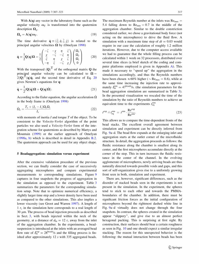
5 Beadaggregation: simulation versus experiment
After the extensive validation procedure of the previous
section, we can finally consider the case of successively
aggregating microspheres and compare experimental
measurements to corresponding simulations. Figure 9
captures in four snapshots the progress of aggregation in
the simulation as opposed to the experiment. Table 3
summarizes the parameters for the corresponding simula-
tion setup. Note that to optimize numerical efficiency, a
slightly larger time step and a lower density have been used
as compared to the other simulations. This also implies a
lower viscosity (see Groot and Warren 1997). A length of
1 rc in the simulation here corresponds to a real length of
30 lm. The process of bead injection proceeds as described
in Sect. 3, with beads injected within the neck of the
geometry, at a distance of dbi = 12 rc away from the inlet
of the aggregation chamber. In the experiments, a bead-
suspension is introduced at the inlets with an averaged bead
flow rate of Ibiexp = 28beads/s and the filling process is fin-
ished after approximately 12 s with 335 aggregated beads.
The maximum Reynolds number at the inlets was Remax ¼5:4 falling down to Remin ¼ 0:7 in the middle of the
aggregation chamber. Similar to the double constriction
considered earlier, we chose a gravitational body force (not
acting on the microspheres) to drive the fluid flow. A
simulation with a maximum time step of dt = 0.03 would
require in our case the calculation of roughly 1.2 million
iterations. However, due to the computer access available
we had to guarantee that the whole filling process can be
calculated within 1 week on 32 processors, distributed over
several time slices (a brief sketch of the coding and com-
puter platforms employed is given in Appendix A). This
made it necessary to ‘‘speed up’’ the aggregation in the
simulations accordingly, and thus the Reynolds numbers
have been chosen &60% higher (�Remax ¼ 8:6), while at
the same time increasing the injection rate to approxi-
mately Ibisim = 47beads/s. (the simulation parameters for the
bead aggregation simulation are summarized in Table 3).
In the presented visualization we rescaled the time of the
simulation by the ratio of Reynolds numbers to achieve an
equivalent time to the experiments teqsim
texp ¼ tsimeq ¼ tsim � Reexp
Resim: ð23Þ
This allows us to compare the time-dependent fronts of the
bead stacks. The excellent overall agreement between
simulation and experiment can be directly inferred from
Fig. 9a–d. The bead flow expands at the enlarging inlet and
aggregation starts at the outlet corner of the microfluidic
structure. In detail, the aggregation proceeds as follows: the
fluidic resistance along the chamber is smallest along its
center, and the first microspheres accumulate directly at the
corner of the step. This in turn increases the fluidic resis-
tance in the center of the channel. In the evolving
agglomerate of microspheres, newly arriving beads are thus
naturally directed towards possible voids and gaps, and this
sort of self-organization gives rise to a uniformly growing
front seen in both, simulation and experiment.
There are, however, significant differences, such as the
disorder of stacked beads seen in the experiments is not
present in the simulation. In the experiment, the spheres
tend to stick to each other and towards the PMMA-
boundaries of the chamber. In addition, there must be
significant friction forces as the initial configuration of
microspheres beyond the rightmost dashed white line in
Fig. 9a–d virtually does not change through the four
snapshots. In contrast, the spheres created in the simulation
appear ‘‘slippery’’, and give rise to an almost perfect
hexagonal packing. This is surprising at first sight. By
construction, their surfaces should bear a certain roughness
as seen in Fig. 10 and one should expect a similar irregular
stacking. The reason for this unexpected behavior is the
following: the mutual interaction between beads has been
Microfluid Nanofluid (2009) 7:307–323 317
123
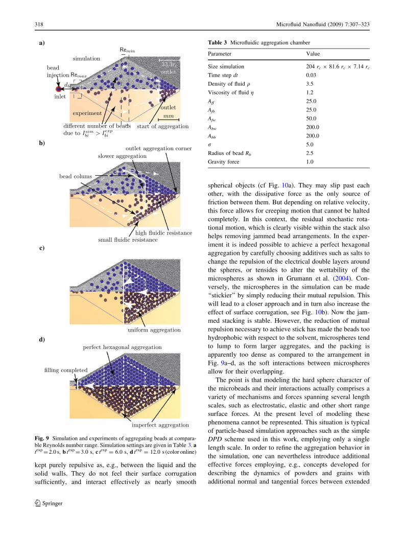
kept purely repulsive as, e.g., between the liquid and the
solid walls. They do not feel their surface corrugation
sufficiently, and interact effectively as nearly smooth
spherical objects (cf Fig. 10a). They may slip past each
other, with the dissipative force as the only source of
friction between them. But depending on relative velocity,
this force allows for creeping motion that cannot be halted
completely. In this context, the residual stochastic rota-
tional motion, which is clearly visible within the stack also
helps removing jammed bead arrangements. In the exper-
iment it is indeed possible to achieve a perfect hexagonal
aggregation by carefully choosing additives such as salts to
change the repulsion of the electrical double layers around
the spheres, or tensides to alter the wettability of the
microspheres as shown in Grumann et al. (2004). Con-
versely, the microspheres in the simulation can be made
‘‘stickier’’ by simply reducing their mutual repulsion. This
will lead to a closer approach and in turn also increase the
effect of surface corrugation, see Fig. 10b). Now the jam-
med stacking is stable. However, the reduction of mutual
repulsion necessary to achieve stick has made the beads too
hydrophobic with respect to the solvent, microspheres tend
to lump to form larger aggregates, and the packing is
apparently too dense as compared to the arrangement in
Fig. 9a–d, as the soft interactions between microspheres
allow for their overlapping.
The point is that modeling the hard sphere character of
the microbeads and their interactions actually comprises a
variety of mechanisms and forces spanning several length
scales, such as electrostatic, elastic and other short range
surface forces. At the present level of modeling these
phenomena cannot be represented. This situation is typical
of particle-based simulation approaches such as the simple
DPD scheme used in this work, employing only a single
length scale. In order to refine the aggregation behavior in
the simulation, one can nevertheless introduce additional
effective forces employing, e.g., concepts developed for
describing the dynamics of powders and grains with
additional normal and tangential forces between extended
a)
b)
c)
d)
Fig. 9 Simulation and experiments of aggregating beads at compara-
ble Reynolds number range. Simulation settings are given in Table 3. atexp = 2.0 s, b texp = 3.0 s, c texp = 6.0 s, d texp = 12.0 s (color online)
Table 3 Microfluidic aggregation chamber
Parameter Value
Size simulation 204 rc 9 81.6 rc 9 7.14 rc
Time step dt 0.03
Density of fluid q 3.5
Viscosity of fluid g 1.2
Aff 25.0
Afb 25.0
Afw 50.0
Abw 200.0
Abb 200.0
r 5.0
Radius of bead Rb 2.5
Gravity force 1.0
318 Microfluid Nanofluid (2009) 7:307–323
123

objects (Cundall and Strack 1979; Luding 2005). An
implementation of a new type of force will in general
introduce another length scale to the system, possibly with
correspondingly reduced integration time steps. On the
other hand, these forces may act only between a relatively
small number of objects, compared to the total number of
particles constituting the simulation such that the overall
numerical efficiency is not affected.
6 Conclusion
To our knowledge this has been the first time a DPD
simulation scheme has been put to the test in a realistic
design used for constructing an actual microfluidic device.
We find that using the method as a separate tool (not
numerically linked to a CFD-scheme) is most efficient, as
hydrodynamics, solid boundaries and interacting dispersed
objects are all treated under one wing. The resulting ver-
satility is clearly a strength of the method. For representing
the problem of the bead assay, we have used a rather
simple version of DPD which is essentially the one
described in Groot and Warren (1997). The purpose was to
show the nature of the simulation method, its virtues and
also its limitations. In the process of validation it has
become apparent that hydrodynamics in channels and with
dispersed interacting objects is represented faithfully, even
without exercising excessive care in setting up the simu-
lation—flow fields and drag forces are represented up to
residual statistical errors, at the channel boundaries the
no-slip boundary condition is obeyed without additional
effort. Only the accurate prescription of pressure boundary
conditions (possibly at various terminals) still remains a
technical challenge.
One may summarize that for laminar flows, one has a
reliable, explicit model for the solvent that may host a
variety of structured objects—these may represent
polymers, vesicles or colloids or beads, and the full
hydrodynamic interactions between them are included.
Carrying out a conscious validation process as outlined in
this work permits to identify precisely the limitations of the
particular scheme used. In our case this has been the lack of
representing multiple length scales or equivalently, a lack
of specialized effective interactions. These, however, may
be added successively in order to emulate the required
behavior. In fact, thinking in terms of successive approxi-
mations by refining force laws might play a major role for
designing future commercial products involving DPD. The
necessity of using varying levels of description in the
particle-based method must not be viewed as a deficiency,
but as a strength of the method. One is able to turn distinct
effects on or off, depending on what is to be learned about
the system in question. In this respect, the scheme is a
powerful explorative tool.
Acknowledgments The support of the Landesstiftung Baden-
Wurttemberg (HPC-Project) is gratefully acknowledged.
Appendix A: Coding and computer platforms
For simulating the types problems presented in this work
we developed a parallelized simulation code based
domains, and each domain is associated with a computa-
tional node (processor or processor core). Since the DPD
interparticle interaction is of relatively short range, a given
domain need only know about the particles within a thin (of
the order of 1 rc) adjacent border of neighboring domains.
That is, most of the time a given process unit can work
quite autonomously. This behavior is most easily imple-
mented with only elementary routines of the Message
Passing Interface (MPI). MPI is available on nearly every
hardware platform ranging from single laptops up to huge
cluster systems with hundreds of processors (Dongarra
et al. 1994). In coding our applications, we essentially
follow Griebel et al. (2004). We stick to a strict domain
decomposition, except for treating rigid objects that may be
a)
b)
Fig. 10 a All FPs of the beads are kept purely repulsive, which
generates slip and lead to a regular hexagonal ordering in a suitable
structure. b Adhesive beads interact at the outer limits via attractive
forces while FPs inside the object are repulsive to prevent beads
merging together (color online)
Microfluid Nanofluid (2009) 7:307–323 319
123

much larger than the cutoff radius. As each microsphere in
the simulation is of the same particle configuration, it is
convenient that each process unit has the information of all
objects, facilitating the computation of the forces acting on
a specific microsphere.
We note that useful information about the problem can
already be extracted from a typical simulation run taking
10–12 h on a cluster with 32 processors. This involves,
e.g., the aggregation of a swarm of beads traversing the
chamber simultaneously. The corresponding computational
resources should be available at almost every research
facility nowadays. The presented sequential filling of beads
takes about 6 days on 32 processors with up to 650,000
time steps and 500,000 FPs on a Linux cluster (NEC Xeon
EM64T) of the high performance computing center in
Stuttgart (http://www.hlrs.de). The issue of size, i.e., the
number of DPD particles needed to represent a certain sit-
uation, which played a role in this work, may soon lose
importance. Low-cost workstations with 4 processors and
16 cores will become standard soon, and the simulations
carried out in this work will not even require a PC-cluster,
and one could also dispose of some of the tricks (reduction
to periodic boundary conditions, bead injector) necessary
in the present work to enhance numerical efficiency.
Appendix B: Simulation algorithm
B1: Velocity-Verlet algorithm for DPD
In the conventional Velocity-Verlet algorithm for conser-
vative forces, there are three stages (Allen and Tildesley
1987; Swope et al. 1982). First, the positions at time
(t ? Dt) and the mid-step velocity at time ðt þ 12DtÞ are
calculated
rðt þ DtÞ ¼ rðtÞ þ DtvðtÞ þ 1
2mDt2fðtÞ ð24Þ
and then the forces with the positions at time (t ? Dt),
fðt þ DtÞ ¼ fðrðt þ DtÞÞ; ð25Þ
and the new velocity is obtained as
vðt þ DtÞ ¼ vðtÞ þ 1
2mDt fðtÞ þ fðt þ DtÞ½ : ð26Þ
In the DPD scheme the force is velocity-dependent, and a
prediction is needed for the velocity at t ? Dt. If, according
to Groot and Warren (1997) the algorithm is modified with
~vðt þ DtÞ ¼ vðtÞ þ kDtfðtÞfðt þ DtÞ ¼ fðrðt þ DtÞ; ~vðt þ DtÞÞ
ð27Þ
time steps up to Dt = 0.05 with sufficient temperature
control. The influence of the integration scheme and the
behavior of a particular system with respect to the time step
has been discussed in Peters (2004) and references therein.
B2: Velocity-Verlet algorithm for quaternions
It is assumed that there exists one coordinate system XYZ
fixed in an inertial frame and an individual body-centered
coordinate systems xyzk fixed in their center of mass (CM).
At first, the position rCMk of the bead k, its mid-point
velocity vCMk and its mid-point angular velocity Xk
CM is
calculated to
rkCMðt þ DtÞ ¼ rk
CMðtÞ þ vkCMðtÞDt þ Dt2
2
fkCMðtÞmk
CM
ð28Þ
vkCMðt þ
1
2DtÞ ¼ vk
CMðtÞ þDt
2
fkCMðtÞmk
CM
ð29Þ
XkCMðt þ
1
2DtÞ ¼ Xk
CMðtÞ þ1
2_X
k
CMðtÞDt ð30Þ
Here mkCM ¼
Pmi and fCM
k = fi are the total mass of
bead k and the total force acting on it. Position and velocity
of the bead are calculated with respect to the laboratory
frame XYZ whereas the angular velocity is calculated with
respect to its body centered frame xyzk.
In the second step the total force fCMk acting on the bead
is calculated by summing-up all forces fi of the FPs inside
the bead that are previously calculated in the Velocity-
Verlet algorithm for FPs (cf Sect. 2).
fkCMðt þ DtÞ ¼
Xnatk
i¼1
f iðt þ DtÞ ð31Þ
In a last step the velocity as well as the angular velocity
of the beads are updated to time (t ? Dt).
vkCMðt þ DtÞ ¼ vk
CMðt þ1
2DtÞ þ Dt
2
fkCMðt þ DtÞ
mkCM
ð32Þ
XðnÞx ðt þ DtÞ ¼ XxðtÞ þDt
2Ix
nTxðtÞ þ Txðt þ DtÞ
þðIy � IzÞ XyðtÞXzðtÞh
þXðn�1Þy ðt þ DtÞXðn�1Þ
z ðt þ DtÞio
ð33Þ
Here the angular velocity is updated via an iterative
procedure in n using Omelyan’s scheme (cyclic with y and
z) where only 3–5 iterations are sufficient to gain good
results for the current time step (Omelyan 1998).
After the dynamics of the whole object k is calculated the
new positions and velocities of the FPs inside the bead have
to be updated with respect to its COM. Because the FPs are
updated in the inertial frame their relative positions Dki and
angular velocities Xk in the body-centered frame first have
320 Microfluid Nanofluid (2009) 7:307–323
123

to be transformed back with the transposed of the rotational
matrix ATðqÞ into the laboratory frame (cf Eq. 19).
rki;relðt þ DtÞ ¼ Ak
Tqkðt þ DtÞ
� Dki ð34Þ
xkCMðt þ
1
2DtÞ ð35Þ
Ak T
qkðt þ DtÞ
�Xk t þ 1
2Dt
� �ð36Þ
With the relative position rki,rel and the angular velocity
xkCM in the inertial frame the position and velocities in the
inertial frame are updated to
rki ðt þ DtÞ ¼ rk
CMðt þ DtÞ þ rki;relðt þ DtÞ ð37Þ
vki t þ 1
2Dt
� �¼ vk
CM t þ 1
2Dt
� �þ xk
CM t þ 1
2Dt
� �
� rki;relðt þ DtÞ ð38Þ
References
Abraham FF (1970) Functional dependence of drag coefficient of a
sphere on reynolds number. Phys Fluids 13(8):2194
Allen MP, Tildesley DJ (1987) Computer simulation of liquids.
Oxford University Press, Oxford
Auroux PA, Iossifidis D, Reyes DR, Manz A (2002) Micro total
analysis systems. Part 2. Analytical standard operations and
applications. Anal Chem 74(12):2637–2652
Bird RB, Stewart WE, Lightfoot EN (2002) Transport phenomena,
2nd edn. Wiley, New York
Boek ES, Coveney PV, Lekkerkerker HNW, vanderSchoot P (1997)
Simulating the rheology of dense colloidal suspensions using
dissipative particle dynamics. Phys Rev E 55(3):3124–3133
Chester W, Breach DR, Proudman I (1969) On flow past a sphere at
low reynolds number. J Fluid Mech 37:751
Christodoulides N, Tran M, Floriano PN, Rodriguez M, Goodey A,
Ali M, Neikirk D, McDevitt JT (2002) A microchip-based
multianalyte assay system for the assessment of cardiac risk.
Anal Chem 74(13):3030–3036
Clark AT, Lal M, Ruddock JN, Warren PB (2000) Mesoscopic
simulation of drops in gravitational and shear fields. Langmuir
16(15):6342–6350
Cundall PA, Strack ODL (1979) A discrete numerical model for
granular assemblies. Geotechnique 29(1):47–65
De Fabritiis G, gado-Buscalioni R, Coveney PV (2006) Multiscale
modeling of liquids with molecular specificity. Phys Rev Lett
97(13)
Dittrich PS, Schwille P (2003) An integrated microfluidic system for
reaction, high-sensitivity detection, and sorting of fluorescent
cells and particles. Anal Chem 75(21):5767–5774
Dongarra J, Walker D, Lusk E, Knighten B, Snir M, Geist A, Otto S,
Hempel R, Lusk E, Gropp W, Cownie J, Skjellum T, Clarke L,
Littlefield R, Sears M, Husslederman S, Anderson E, Berryman
S, Feeney J, Frye D, Hart L, Ho A, Kohl J, Madams P, Mosher C,
Pierce P, Schikuta E, Voigt RG, Babb R, Bjornson R, Fernando
V, Glendinning I, Haupt T, Ho CTH, Krauss S, Mainwaring A,
Nessett D, Ranka S, Singh A, Weeks D, Baron J, Doss N,
Fineberg S, Greenberg A, Heller D, Howell G, Leary B,
Mcbryan O, Pacheco P, Rigsbee P, Sussman A, Wheat S,
Barszcz E, Elster A, Flower J, Harrison R, Henderson T,
Kapenga J, Maccabe A, Mckinley P, Palmer H, Robison A,
Tomlinson R, Zenith S (1994) Special issue - mpi - a message-
passing interface standard. Int J Supercomput Appl High
Perform Comput 8(3-4):165
Doyle PS, Bibette J, Bancaud A, Viovy JL (2002) Self-assembled
magnetic matrices for dna separation chips. Science
295(5563):2237–2237
Ducree J, Zengerle R (2004) FlowMap—microfluidics roadmap for the
life sciences. Books on demand GmbH, Norderstedt, Germany
Duong TT, Kim G, Ros R, Streek M, Schmid F, Brugger J, Anselmetti
D, Ros A (2003) Size-dependent free solution dna electropho-
resis in structured microfluidic systems. Microelectron Eng 67-
8:905–912
Dupin MM, Halliday I, Care CM (2006) Simulation of a flow
focusing device. Phys Rev E 73:055701
Espanol P (1995) Hydrodynamics from dissipative particle dynamics.
Phys Rev E 52(2):1734–1742
Espanol P (1998) Fluid particle model. Phys Rev E 57(3):2930–2948
Espanol P, Revenga M (2003) Smoothed dissipative particle dynam-
ics. Phys Rev E 67(2)
Espanol P, Warren PB (1995) Statistical-mechanics of dissipative
particle dynamics. Europhys Lett 30(4):191–196
Evans DJ (1977) Representation of orientation space. Mol Phys
34(2):317–325
Evans DJ, Murad S (1977) Singularity free algorithm for molecular-
dynamics simulation of rigid polyatomics. Mol Phys 34(2):327–
331
Frisch U, Hasslacher B, Pomeau Y (1986) Lattice-gas automata for
the navier-stokes equation. Phys Rev Lett 56(14):1505–1508
Glatzel T, Cupelli C, Kuester U, Zengerle R, Santer M (2006a)
Aggregating beads in microfluidic chambers on high perfor-
mance computers compared to experiments. In: 10th anniversary
international conference on miniaturized systems for chemistry
and life sciences (lTAS), pp 53–55
Glatzel T, Cupelli C, Kuester U, Zengerle R, Santer M (2006b)
Simulation of aggregating beads in microfluidics on high
performance computers with a fluid particle approach. In:
International conference multiscale materials modeling
(MMM), pp 54–56
Goldstein H (1980) Classical mechanics, 2nd edn. Addison-Wesley,
Reading
Griebel M, Knapek S, Zumbusch G, Caglar A (2004) Numerische
Simulationen in der Molekuldynamik. Springer, Berlin
Groot RD, Madden TJ (1998) Dynamic simulation of diblock
copolymer microphase separation. J Chem Phys 108(20):8713–
8724
Groot RD, Rabone KL (2001) Mesoscopic simulation of cell
membrane damage, morphology change and rupture by nonionic
surfactants. Biophys J 81(2):725–736
Groot RD, Warren PB (1997) Dissipative particle dynamics: Bridging
the gap between atomistic and mesoscopic simulation. J Chem
Phys 107(11):4423–4435
Grumann M, Dobmeier M, Schippers P, Brenner T, Kuhn C, Fritsche
M, Zengerle R, Ducree J (2004) Aggregation of bead-monolay-
ers in flat microfluidic chambers simulation by the model of
porous media. Lab Chip 4(3):209–213
Grumann M, Geipel A, Riegger L, Zengerle R, Ducree J (2005)
Batch-mode mixing on centrifugal microfluidic platforms. Lab
Chip 5(5):560–565
Haeberle S, Zengerle R (2007) Microfluidic platforms for Lab-On-A-
Chip applications. Lab Chip 7:1094–1110
Haeberle S, Zengerle R, Ducree J (2007) Centrifugal generation and
manipulation of droplet emulsions. Microfluid Nanofluidics
3:65–75
Hardt S, Schonfeld F (2003) Laminar mixing in different interdigital
micromixers. Part II. Numerical simulations. AIChE J
49(3):578–584
Microfluid Nanofluid (2009) 7:307–323 321
123

Harrison DJ, Wang C, Thibeault P, Ouchen F, Cheng S (2000) The
decade’s search for the killer ap in l tas. In: Proceedings of
the l Tas 2000 Symposium. Kluwer, pp 195–204
Henrich B, Cupelli CG, Moseler M, Santer M (2007) An adhesive dpd
wall model for dynamic wetting. Europhys Lett 80:60004
Hessel V, Hardt S, Lowe H, Schonfeld F (2003) Laminar mixing in
different interdigital micromixers. Part I. Experimental charac-
terization. AIChE J 49(3):566–577
Heyes DM, Baxter J, Tuzun U, Qin RS (2004) Discrete-element
method simulations: from micro to macro scales. Phil Trans R
Soc Lond A 362:1853–1865
Hoogerbrugge PJ, Koelman JMVA (1992) Simulating microscopic
hydrodynamic phenomena with dissipative particle dynamics.
Europhys Lett 19(3):155–160
Johnson RW (1998) The handbook of fluid dynamics. Springer,
Heidelberg
Keaveny EE, Pivkin IV, Maxey M, Karniadakis GE (2005) A
comparative study between dissipative particle dynamics and
molecular dynamics for simple- and complex-geometry flows. J
Chem Phys 123(10)
Kerby MB, Spaid M, Wu S, Parce JW, Chien RL (2002) Selective ion
extraction: a separation method for microfluidic devices. Anal
Chem 74(20):5175–5183
Kim JM, Phillips RJ (2004) Dissipative particle dynamics simulation
of flow around spheres and cylinders at finite reynolds numbers.
Chem Eng Sci 59(20):4155–4168
Koelman JMVA, Hoogerbrugge PJ (1993) Dynamic simulations of
hard-sphere suspensions under steady shear. Europhys Lett
21(3):363–368
Kong B, Yang X (2006) Dissipative particle dynamics simulation of
contact angle hysteresis on a patterned solid/air composite
surface. Langmuir 22(5):2065–2073
Kurita R, Hayashi K, Fan X, Yamamoto K, Kato T, Niwa O (2002)
Microfluidic device integrated with pre-reactor and dual
enzyme-modified microelectrodes for monitoring in vivo glucose
and lactate. Sens Actuators B Chem 87(2):296–303
Kurita R, Yokota Y, Sato Y, Mizutani F, Niwa O (2006a) On-chip
enzyme immunoassay of a cardiac marker using a microfluidic
device combined with a portable surface plasmon resonance
system. Anal Chem 78(15):5525–5531
Kurita R, Yabumoto N, Niwa O (2006b) Miniaturized one-chip
electrochemical sensing device integrated with a dialysis mem-
brane and double thin-layer flow channels for measuring blood
samples. Biosens Bioelectron 21(8):1649–1653
Landau LD, Lifshitz EM (2004) Course of theoretical physics. Fluid
mechanics, vol 6. Butterworth Heinemann
Lettieri GL, Dodge A, Boer G, de Rooij NF, Verpoorte E (2003) A
novel microfluidic concept for bioanalysis using freely moving
beads trapped in recirculating flows. Lab Chip 3(1):34–39
Li J, Liao DY, Yip S (1998) Coupling continuum to molecular-
dynamics simulation: reflecting particle method and the field
estimator. Phys Rev E 57(6):7259–7267
Li PCH, Wang WJ, Parameswaran M (2003) An acoustic wave sensor
incorporated with a microfluidic chip for analyzing muscle cell
contraction. Analyst 128(3):225–231
Lowe CP (1999) An alternative approach to dissipative particle
dynamics. Europhys Lett 47(2):145–151
Luding S (2005) Anisotropy in cohesive, frictional granular media. J
Phys Condens Matter 17(24):S2623–S2640
MacDonald MP, Spalding GC, Dholakia K (2003) Microfluidic
sorting in an optical lattice. Nature 426(6965):421–424
Marsh CA, Backx G, Ernst MH (1997) Static and dynamic properties
of dissipative particle dynamics. Phys Rev E 56(2):1676–1691
Martys NS, Mountain RD (1999) Velocity verlet algorithm for
dissipative-particle-dynamics-based models of suspensions. Phys
Rev E 59(3):3733–3736
Masters AJ, Warren PB (1999) Kinetic theory for dissipative particle
dynamics: the importance of collisions. Europhys Lett 48(1):1–7
Monaghan JJ (1992) Smoothed particle hydrodynamics. Annu Rev
Astron Astrophys 30:543–574
Monaghan JJ (2005) Smoothed particle hydrodynamics. Rep Prog
Phys 68(8):1703–1759
Nicholson D, Cracknell RF, Quirke N (1995) Direct molecular
dynamics simulation of flow down a chemical potential gradient
in a slit-shaped micropore. Phys Rev Lett 74(13):2463
Omelyan IP (1998a) On the numerical integration of motion for rigid
polyatomics: The modified quaternion approach. Comput Phys
12(1):97–103
Omelyan IP (1998b) Algorithm for numerical integration of the rigid-
body equations of motion. Phys Rev E 58(1):1169–1172
Oosterbroek RE, van den Berg A (2003) Lab-on-a-Chip: miniaturized
systems for (bio)chemical analysis and synthesis. Elsevier,
Amsterdam
Pagonabarraga I, Frenkel D (2001) Dissipative particle dynamics for
interacting systems. J Chem Phys 115(11):5015–5026
Peters EAJF (2004) Elimination of time step effects in dpd. Europhys
Lett 66(3):311–317
Pivkin IV, Karniadakis GE (2006) Coarse-graining limits in open and
wall-bounded dissipative particle dynamics systems. J Chem
Phys 124(18)
Proudman I, Pearson JRA (1957) Expansions at small reynolds
numbers for the flow past a sphere and a circular cylinder. J Fluid
Mech 2(3):237–262
Pryamitsyn V, Ganesan V (2005) A coarse-grained explicit solvent
simulation of rheology of colloidal suspensions. J Chem Phys
122(10)
Revenga M, Zuniga I, Espanol P, Pagonabarraga I (1998) Boundary
models in dpd. Int J Mod Phys C 9(8):1319–1328
Revenga M, Zuniga I, Espanol P (1999) Boundary conditions in
dissipative particle dynamics. Comput Phys Commun 122:309–
311
Reyes DR, Iossifidis D, Auroux PA, Manz A (2002) Micro total
analysis systems. Part 1. Introduction, theory, and technology.
Anal Chem 74(12):2623–2636
Riegger L, Markus Grumann, Nann T, Riegler J, Ehlert O,
Mittenbuhler K, Urban G, Pastewka L, Brenner T, Zengerle R,
Ducree J (2006) Read-out concepts for multiplexed bead-based
fluorescence immunoassays on centrifugal microfluidic plat-
forms. Sens Actuators A Phys 126:455–462
Ripoll M, Ernst MH, Espanol P (2001) Large scale and mesoscopic
hydrodynamics for dissipative particle dynamics. J Chem Phys
115(15):7271–7284
Roos P, Skinner CD (2003) A two bead immunoassay in a micro
fluidic device using a flat laser intensity profile for illumination.
Analyst 128(6):527–531
Saleh OA, Sohn LL (2003) Direct detection of antibody-antigen
binding using an on-chip artificial pore. Proc Natl Acad Sci USA
100(3):820–824
Sanders JC, Breadmore MC, Kwok YC, Horsman KM, Landers JP
(2003) Hydroxypropyl cellulose as an adsorptive coating sieving
matrix for dna separations: artificial neural network optimization
for microchip analysis. Anal Chem 75(4):986–994
Sato K, Kitamori T (2004) Integration of an immunoassay system into
a microchip for high-throughput assay. J Nanosci Nanotechnol
4(6):575–579
Sato K, Yamanaka M, Takahashi H, Tokeshi M, Kimura H, Kitamori
T (2002) Microchip-based immunoassay system with branching
multichannels for simultaneous determination of interferon-
gamma. Electrophoresis 23(5):734–739
Sbragaglia M, Benzi R, Biferale L, Succi S, Sugiyama K, Toschi F
(2007) Generalized lattice boltzmann method with multirange
pseudopotential. Phys Rev E 75:026702
322 Microfluid Nanofluid (2009) 7:307–323
123

Sohn YS, Goodey A, Anslyn EV, McDevitt JT, Shear JB, Neikirk DP
(2005) A microbead array chemical sensor using capillary-based
sample introduction: toward the development of an electronic
tongue. Biosens Bioelectron 21(2):303–312
Stone HA, Stroock AD, Ajdari A (2004) Engineering flows in small
devices: microfluidics toward a lab-on-a-chip. Annu Rev Fluid
Mech 36:381–411
Sugiura S, Oda T, Izumida Y, Aoyagi Y, Satake M, Ochiai A,
Ohkohchi N, Nakajima M (2005) Size control of calcium
alginate beads containing living cells using micro-nozzle array.
Biomaterials 26(16):3327–3331
Sun M, Ebner C (1992) Molecular-dynamics simulation of com-
pressible fluid-flow in 2-dimensional channels. Phys Rev A
46(8):4813–4818
Swope WC, Andersen HC, Berens PH, Wilson KR (1982) A
computer-simulation method for the calculation of equilibrium-
constants for the formation of physical clusters of molecules—
application to small water clusters. J Chem Phys 76(1):637–649
Tabuchi M, Ueda M, Kaji N, Yamasaki Y, Nagasaki Y, Yoshikawa K,
Kataoka K, Baba Y (2004) Nanospheres for dna separation
chips. Nat Biotechnol 22(3):337–340
Tian HJ, Landers JP (2002) Hydroxyethylcellulose as an effective
polymer network for dna analysis in uncoated glass microchips:
optimization and application to mutation detection via hetero-
duplex analysis. Anal Biochem 309(2):212–223
Tian HJ, Huhmer AFR, Landers JP (2000) Evaluation of silica resins for
direct and efficient extraction of dna from complex biological
matrices in a miniaturized format. Anal Biochem 283(2):175–191
Trofimov SY (2003) Thermodynamic consistency in dissipative
particle dynamics, thesis/dissertation. Technische Universiteit
Eindhoven, Eindhoven
Vandyke M (1971) Comments on functional dependence of drag
coefficient of a sphere on reynolds number. Phys Fluids
14(5):1038–1039
Vattulainen I, Karttunen M, Besold G, Polson JM (2002) Integration
schemes for dissipative particle dynamics simulations: from
softly interacting systems towards hybrid models. J Chem Phys
116(10):3967–3979
Vilkner T, Janasek D, Manz A (2004) Micro total analysis systems:
recent developments. Anal Chem 76(12):3373–3385
Warren PB (2003) Vapor-liquid coexistence in many-body dissipative
particle dynamics. Phys Rev E 68(6)
Wolff A, Perch-Nielsen IR, Larsen UD, Friis P, Goranovic G, Poulsen
CR, Kutter JP, Telleman P (2003) Integrating advanced func-
tionality in a microfabricated high-throughput fluorescent-
activated cell sorter. Lab Chip 3(1):22–27
Yakovleva J, Davidsson R, Lobanova A, Bengtsson M, Eremin S,
Laurell T, Emneus J (2002) Microfluidic enzyme immunoassay
using silicon microchip with immobilized antibodies and
chemiluminescence detection. Anal Chem 74(13):2994–3004
Yakovleva J, Davidsson R, Bengtsson M, Laurell T, Emneus J
(2003a) Microfluidic enzyme immunosensors with immobilised
protein a and g using chemiluminescence detection. Biosens
Bioelectron 19(1):21–34
Yakovleva J, Zherdev AV, Popova VA, Eremin SA, Dzantiev BB
(2003b) Production of antibodies and development of enzyme-
linked immunosorbent assays for the herbicide butachlor.
Analytica Chimica Acta 491(1):1–13
Yoshida M, Tohda K, Gratzl M (2003) Hydrodynamic micromanipu-
lation of individual cells onto patterned attachment sites on
biomicroelectromechanical system chips. Anal Chem
75(17):4686–4690
Microfluid Nanofluid (2009) 7:307–323 323
123