Simulation of Leveraged ETF Volatility UsingNonparametric Density Estimation

Matthew Ginley

May 20th, 2016

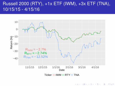
Russell 2000 (RTY), +1x ETF (IWM), +3x ETF (TNA),10/15/15 - 4/15/16

RRTY = − 2.74%RIWM = − 2.7%

RTNA = − 12.52%−40

−30

−20

−10

0

10

11/1/15 12/1/15 1/1/16 2/1/16 3/1/16 4/1/16Date

Ret

urn

(%)

Ticker IWM RTY TNA

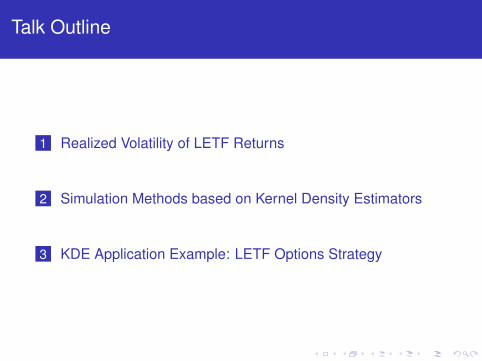
Talk Outline

1 Realized Volatility of LETF Returns

2 Simulation Methods based on Kernel Density Estimators

3 KDE Application Example: LETF Options Strategy

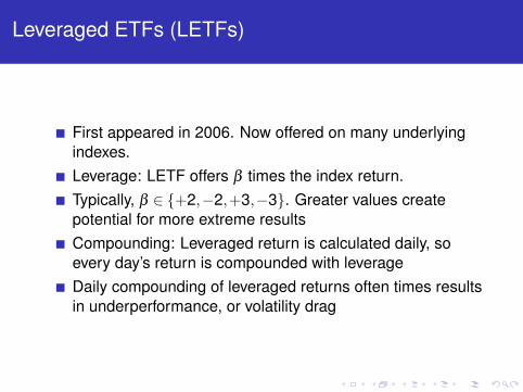
Leveraged ETFs (LETFs)

First appeared in 2006. Now offered on many underlyingindexes.Leverage: LETF offers β times the index return.Typically, β ∈ {+2,−2,+3,−3}. Greater values createpotential for more extreme resultsCompounding: Leveraged return is calculated daily, soevery day’s return is compounded with leverageDaily compounding of leveraged returns often times resultsin underperformance, or volatility drag

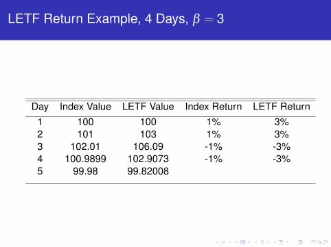
LETF Return Example, 4 Days, β = 3

Day Index Value LETF Value Index Return LETF Return1 100 100 1% 3%2 101 103 1% 3%3 102.01 106.09 -1% -3%4 100.9899 102.9073 -1% -3%5 99.98 99.82008

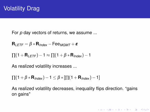
Volatility Drag

For p day vectors of returns, we assume ...

RLETF = β ∗RIndex −FeeMGMT + εεε

∏(1+RLETF )−1≈∏(1+β ∗RIndex)−1

As realized volatility increases ...

∏(1+β ∗RIndex)−1≤ β ∗ [∏(1+RIndex)−1]

As realized volatility decreases, inequality flips direction. “gainson gains"

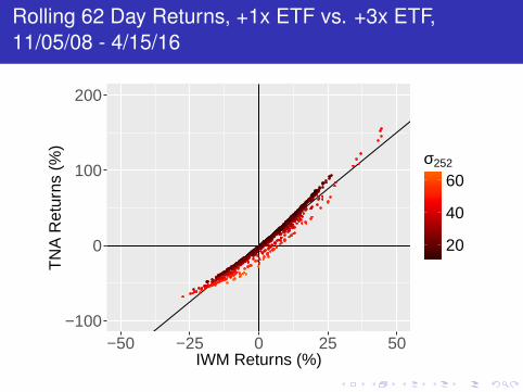
Rolling 62 Day Returns, +1x ETF vs. +3x ETF,11/05/08 - 4/15/16

−100

0

100

200

−50 −25 0 25 50IWM Returns (%)

TN

A R

etur

ns (

%)

20

40

60σ252

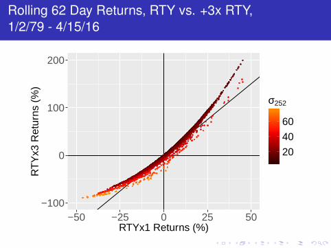
Rolling 62 Day Returns, RTY vs. +3x RTY,1/2/79 - 4/15/16

−100

0

100

200

−50 −25 0 25 50RTYx1 Returns (%)

RT

Yx3

Ret

urns

(%

)

20

40

60

σ252

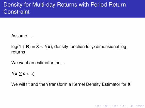
Density for Multi-day Returns with Period ReturnConstraint

Assume ...

log(1+R) = X∼ f (x), density function for p dimensional logreturns

We want an estimator for ...

f (x|∑x < c)

We will fit and then transform a Kernel Density Estimator for X

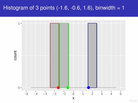
Histogram of 3 points (-1.6, -0.6, 1.6), binwidth = 1

0

1

−5 −4 −3 −2 −1 0 1 2 3 4 5x

coun

t

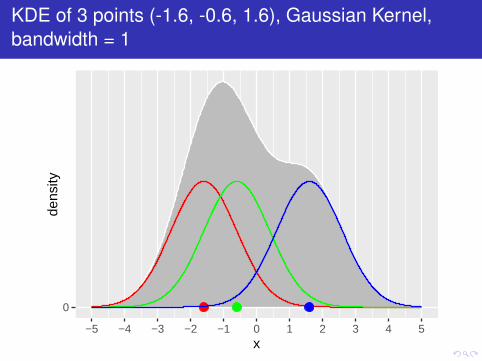
KDE of 3 points (-1.6, -0.6, 1.6), Gaussian Kernel,bandwidth = 1

0

−5 −4 −3 −2 −1 0 1 2 3 4 5x

dens

ity

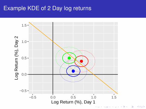
Example KDE of 2 Day log returns

−0.5

0.0

0.5

1.0

1.5

−0.5 0.0 0.5 1.0 1.5Log Return (%), Day 1

Log

Ret

urn

(%),

Day

2

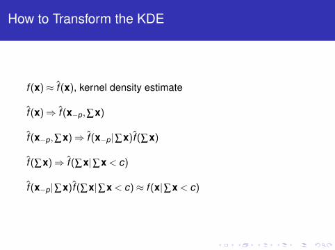
How to Transform the KDE

f (x)≈ f̂ (x), kernel density estimate

f̂ (x)⇒ f̂ (x−p,∑x)

f̂ (x−p,∑x)⇒ f̂ (x−p|∑x)f̂ (∑x)

f̂ (∑x)⇒ f̂ (∑x|∑x < c)

f̂ (x−p|∑x)f̂ (∑x|∑x < c)≈ f (x|∑x < c)

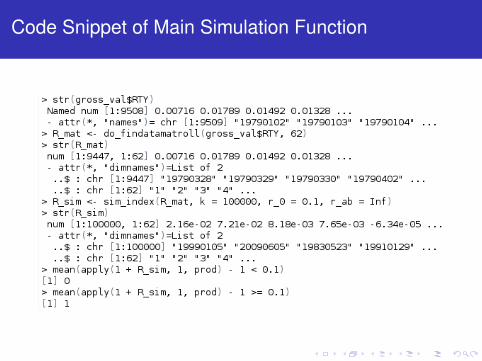
Code Snippet of Main Simulation Function

Key References

“Simulation of Leveraged ETF Volatility UsingNonparametric Density Estimation", Journal ofMathematical Finance, November 2015Proposes constrained KDE and tracking error methods (notrestricted to finance/time series), and LETF volatility example.

“Shortfall from Maximum Convexity", arXiv.org, November2015Appendix/Companion with more insights on realized volatility ofLETF returns and volatility drag.

https://github.com/bonzodroog, mginley@rice.eduAll code for simulation methods, presentation visuals, and Exceltemplates for Bloomberg data.

Dr. Tim Leung, faculty at Columbia University, LETF ExpertContinuous time models of LETF returns, and a whole lot more.

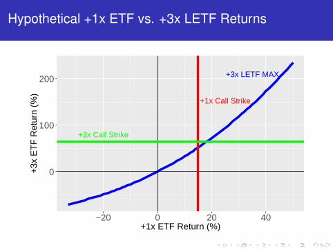
Hypothetical +1x ETF vs. +3x LETF Returns

+1x Call Strike

+3x Call Strike

+3x LETF MAX

0

100

200

−20 0 20 40+1x ETF Return (%)

+3x

ET

F R

etur

n (%

)

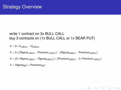
Strategy Overview

write 1 contract on 3x BULL CALLbuy 3 contracts on (1x BULL CALL or 1x BEAR PUT)

V = 3∗V1xBULL−V3xBULL

V = 3∗ (Payout1xBULL−Premium1xBULL)− (Payout3xBULL−Premium3xBULL)

V = (3∗Payout1xBULL−Payout3xBULL)+(Premium3xBULL−3∗Premium1xBULL)

V = PayoutNET +PremiumNET

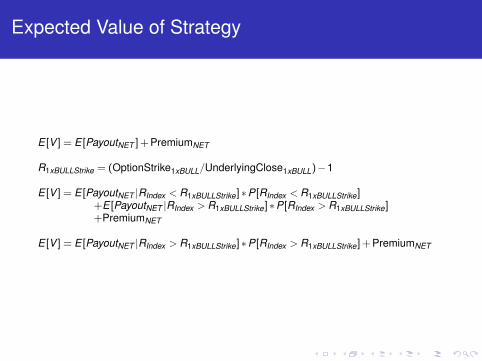
Expected Value of Strategy

E [V ] = E [PayoutNET ]+PremiumNET

R1xBULLStrike = (OptionStrike1xBULL/UnderlyingClose1xBULL)−1

E [V ] = E [PayoutNET |RIndex < R1xBULLStrike]∗P[RIndex < R1xBULLStrike]+E [PayoutNET |RIndex > R1xBULLStrike]∗P[RIndex > R1xBULLStrike]+PremiumNET

E [V ] = E [PayoutNET |RIndex > R1xBULLStrike]∗P[RIndex > R1xBULLStrike]+PremiumNET

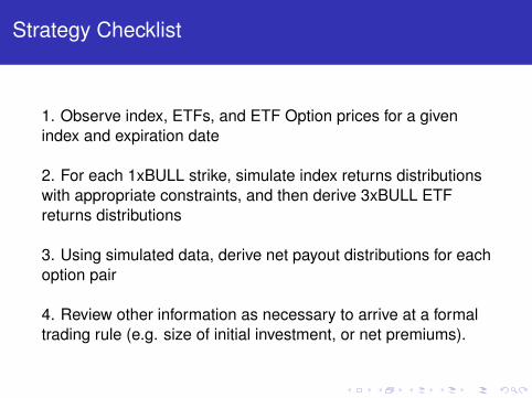
Strategy Checklist

1. Observe index, ETFs, and ETF Option prices for a givenindex and expiration date

2. For each 1xBULL strike, simulate index returns distributionswith appropriate constraints, and then derive 3xBULL ETFreturns distributions

3. Using simulated data, derive net payout distributions for eachoption pair

4. Review other information as necessary to arrive at a formaltrading rule (e.g. size of initial investment, or net premiums).

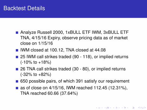
Backtest Details

Analyze Russell 2000, 1xBULL ETF IWM, 3xBULL ETFTNA, 4/15/16 Expiry, observe pricing data as of marketclose on 1/15/16IWM closed at 100.12, TNA closed at 44.0825 IWM call strikes traded (90 - 118), or implied returns(-10% to +18%)26 TNA call strikes traded (30 - 80), or implied returns(-32% to +82%)650 possible pairs, of which 391 satisfy our requirementas of close on 4/15/16, IWM reached 112.45 (12.31%),TNA reached 60.66 (37.64%)

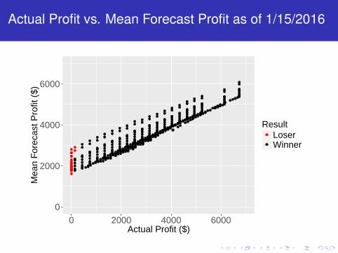
Actual Profit vs. Mean Forecast Profit as of 1/15/2016

0

2000

4000

6000

0 2000 4000 6000Actual Profit ($)

Mea

n F

orec

ast P

rofit

($)

ResultLoserWinner

Wrap Up

KDEs are fast, flexible, and simple. Let the data speak forthemselves.KDEs are a useful tool for analyzing LETFs because oftheir ease of implementation and abundance of Indexreturn data available.R and R Studio make the brainstorming and developmentprocess more productive and enjoyable.

Thanks to R/Finance 2016 and Rice University!

Special thanks to R Studio and Rishi Narang!