UNIVERSITY OF GOTHENBURG

Simulation of model spectra for evaluation of

in vivo magnetic resonance spectra with LCModel

M.Sc. Thesis

Author: Christina Söderman

Supervisors: Ph.D Maria Ljungberg & Ph.D Åsa Carlsson

Department of Radiation Physics

University of Gothenburg

Gothenburg, Sweden

Abstract

LCModel is a software tool for analysis and quantification of in vivo magnetic resonance (MR)

spectra. It estimates the spectrum under evaluation as a linear combination of a set of model

spectra for each metabolite of interest. This thesis describes the work of simulating model spectra

for the point resolved spectroscopy sequence (PRESS) on a 3T MR system, verifying them with

phantom measurements and applying them on in vivo data.

The model spectra were generated by using Vespa-Simulation, which is based on the

GAMMA/PyGAMMA NMR simulation libraries. Six different PRESS echo times (TE:s) were

considered and ideal “hard” RF-pulses were assumed. MR spectroscopy measurements were

performed on a phantom with known concentrations of the metabolites glutamate and creatine.

In vivo measurements were performed on a healthy volunteer in four different regions of the

brain.

Evaluation of the simulated spectra indicated that the timing of the RF-pulses in the PRESS

sequence influences the outcome of the spectra for metabolites containing coupled spins, whereas

uncoupled spins show no such dependence.

The LCModel fit of the simulated model spectra to the phantom measurement data resulted in

non-random residuals. This might be due to effects on the measured data originating from the

actual RF-pulse shapes on the MR system, not accounted for in the simulations. A concentration

calibration factor for the metabolite concentrations given by LCModel, using the simulated basis

sets, was determined to 0.87 ± 2.5 %.

LCModel analysis of the in vivo data, using the simulated model spectra, showed good results for

the fit. Some structure in the residual could be seen in two of the fitted data sets, presumably a

spurious echo artifact or a consequence of the residuals seen in the fit of the phantom data.

Table of contents1 INTRODUCTION 1

1.1 MRS basics................................................................................................................................1

1.2 Vespa-Simulation.....................................................................................................................7

1.3 LCModel basis sets...................................................................................................................8

2 MATERIAL AND METHODS 92.1 Model spectra simulations.......................................................................................................9

2.2 Phantom measurements........................................................................................................14

2.3 Concentration calibration......................................................................................................15

2.4 In vivo measurements............................................................................................................16

3 RESULTS 193.1 Model spectra simulation......................................................................................................19

3.2 Phantom measurements........................................................................................................22

3.3 Concentration calibration......................................................................................................25

3.4 In vivo measurements............................................................................................................25

4 DISCUSSION 28

5 CONCLUSION 31

Acknowledgments 32

References 33

1 INTRODUCTION

In vivo magnetic resonance spectroscopy (MRS) is a non-invasive technique for quantification of

tissue metabolites. One of the areas in which the technique is widely used, is in the research of

brain deceases, e.g. gliomas or dementia[1][2]. The goal of many studies is to correlate an

elevation or decrease of the concentration of a certain metabolite with the unhealthy state. This

approach indicates the need of a reliable MRS analysis tool, with as little user dependence as

possible. LCModel is a well established software for evaluation and quantification of in vivo MR

spectra, where the spectrum under evaluation is estimated as a linear combination of a set of

model spectra for each metabolite of interest[3]. These model spectra form a basis set within

LCModel, and they may be measured in vitro from aqueous metabolite solutions, or may be

quantum-mechanically simulated.

The aim of this work was to create model spectra for a PRESS sequence on a 3T system for

LCModel by means of simulation, to perform phantom measurements for verification and

concentration calibration and to finally apply the model spectra on in vivo data.

1.1 MRS basics1

Atomic nuclei with an odd atomic number posses non zero quantum spin and charge. The spin

puts the charge in motion, resulting in a magnetic field accompanied by a magnetic dipole moment

and magnetization vector. When placed in a strong external magnetic field, the magnetization

vector will precess, or resonate, around the field axis with a frequency ν, called the Larmor or

resonance frequency, given by:

ν=ω/2π=B0⋅γ/2π (1.1)

where ω is the angular frequency in radians per second, B0 is the strength of the magnetic field in

Tesla (T) and γ is the gyromagnetic ratio in Hz/T.

1 This chapter contains basic magnetic resonance spectroscopy theory, which can be found in [4],[5] and [6].

1

A large group of nuclei, for example the 1H nuclei in the human body, placed in a magnetic field will

create a net magnetic field, M0, in the same direction as the main field vector as illustrated in

Figure 1.1. However, to measure this weak M0-field is difficult in the much stronger B0-field. By

applying a radio frequency pulse (RF-pulse), the net magnetization can be exited, i.e. can be

flipped to a plane perpendicular to the B0-field. The magnetization is then said to be in the

transverse plane, see Figure 1.2.

The precession in the transverse plane can be detected as an alternating voltage in a coil. Various

factors will induce a relaxation effect on the transverse magnetization, causing a damped signal

with a decay time referred to as T2*. This signal is called the Free Induction Decay, or FID, and

consists of an x- and y-component which are detected separately, referred to as the real and

imaginary part of the FID respectively, see Figure 1.3.

2

Figure 1.1: When placed in an outer magnetic field, B0, a group of nuclei will create a net magnetization, M0, aligned with the B0.

Figure 1.2: If subjected to a RF pulse, the net magnetization will be flipped to the transverse plane, perpendicular to the B0-field.

Figure 1.3: The real and imaginary part of the FID.

The signal components, Sx(t) and Sy(t), are given by Equations 1.2 and 1.3.

Sx t =S0t [cos 0−t]e−t/T2* (1.2)

Sy (t )=S0(t)[sin(ω0−ω) t+φ]e(−t/T 2*) (1.3)

φ is the phase of the signal and ω0 is a reference angular frequency. The angular frequency

contents of the FID, S(ω), can be extracted with a Fourier transform of the time domain data of the

signal, S(t), according to:

S (ω)=∫−∞

∞

S (t)e(−i ω t)dt=Re(ω )+Im (ω ) (1.4)

Re(ω )=A(ω)cos (φ)−D(ω)sin(φ) (1.5)

Im(ω )=A(ω)sin(φ)+D(ω)cos(φ) (1.6)

where

A(ω)=S0 T 2

*

1+(ω0−ω)2T 2* 2

(1.7)

D(ω)=S0(ω0−ω)T 2

*

1+(ω0−ω)2T 2* 2

(1.8)

A(ω) and D(ω) are the absorption and dispersion components of the signal. The final spectrum is a

plot of the real part of the Fourier transform in the frequency domain, where the area under one

peak is proportional to the number of protons contributing to the signal.

3

When analyzing spectra, it is preferable to work with the peaks originating from the absorption

mode, shown in Figure 1.4. However if φ≠0, the resulting spectrum after Fourier transform will be

a mixture of absorption and dispersion mode, leading to a distorted lineshape as in Figure 1.5.

By doing a zero-order phase correction of the spectrum, so that φ=φc in Equation 1.9, a pure

absorption mode spectrum is achieved.

Re( )=A cos −c−D sin−c (1.9)

The resolution of an MR spectra is given by the Full Width at Half Maximum (FWHM), which is the

width of a peak at half its maximum value.

It is of importance that the acquisition time of the FID is sufficiently long, so that the signal has

time to decay in to noise. If this is not the case, the peaks of the spectrum will be subjected to

truncation artifacts.

The Larmor equation (Equation 1.1) suggest that every nuclei of the same species will resonate

with the same frequency given an outer magnetic field. This is not entirely true. Electrons orbiting

the nuclei will create a magnetic field, which shields the nucleus from the B 0-field. The extent to

which the strength of the B0-field is shielded, depends on the chemical environment of the

nucleus, i.e. the electronic density in its vicinity. The corresponding effect on the resonance

frequency is referred to as the chemical shift. With this in consideration, the resonance frequency

4

Figure 1.5: If the phase of the FID is non-zero, the resulting spectrum will be a mixture of absorption and dispersion mode.

Figure 1.4: The absorption (solid line) and dispersion (dashed line) components of the lineshape.

ν, in Hz, is instead given by:

ν=B0(1−σ)⋅γ/2π (1.10)

where σ is a dimensionless “shielding constant”, describing the effect on the magnetic field from

the electrons. By convention the chemical shift δ is given in parts per million (ppm) relative to a

reference frequency υref, according to

δ=ν−νref

νref

⋅106 (1.11)

MR spectra are in general presented as the signal strength as a function of ppm, with the ppm

range increasing from right to left.

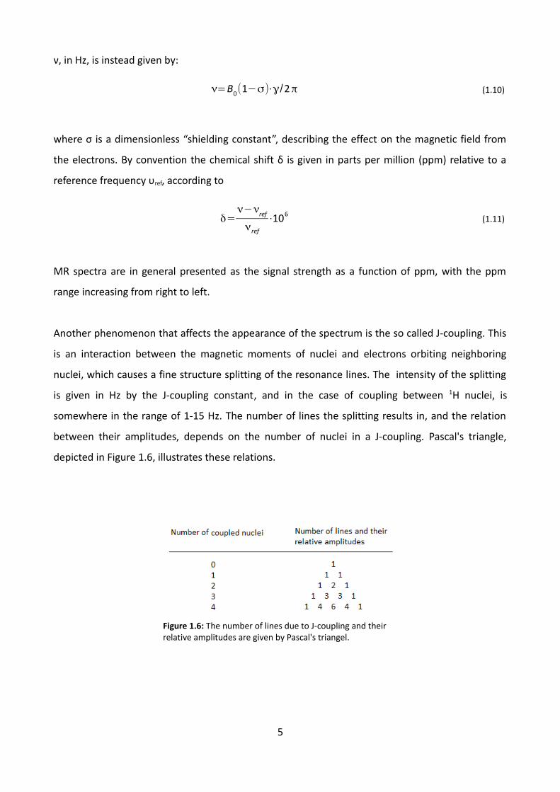
Another phenomenon that affects the appearance of the spectrum is the so called J-coupling. This

is an interaction between the magnetic moments of nuclei and electrons orbiting neighboring

nuclei, which causes a fine structure splitting of the resonance lines. The intensity of the splitting

is given in Hz by the J-coupling constant, and in the case of coupling between 1H nuclei, is

somewhere in the range of 1-15 Hz. The number of lines the splitting results in, and the relation

between their amplitudes, depends on the number of nuclei in a J-coupling. Pascal's triangle,

depicted in Figure 1.6, illustrates these relations.

5

Figure 1.6: The number of lines due to J-coupling and their relative amplitudes are given by Pascal's triangel.

With prior knowledge of the chemical shift and J-coupling constants of metabolites, it is possible to

identify them in human tissue by acquiring signal from a volume of interest (VOI) in the body, e.g. a

small volume of a certain part of the brain. Volume selection is generally achieved by the

application of magnetic field gradients in combination with RF-pulses, the point resolved

spectroscopy sequence (PRESS) is such a method[7]. Figure 1.7 depicts the PRESS sequence

generically.

The PRESS sequence starts of with a 90o RF-pulse that flips the spins to the transverse plane, which

is followed by two RF pulses that flips the spins 180o through the transverse plane. A 180o-pulse

will reverse the phases of the spins, and as they continue to phase evolve in the same direction,

they will be refocused and form a spin echo. By applying a magnetic field gradient over the object,

there will be a variation of the Larmor frequency, see Equation 1.1. Only those spins with

resonances matching the frequency contents of the RF-pulse, will be effected by it. With three RF-

pulses and three orthogonal magnetic field gradients, as in PRESS, the final signal measured is that

from a VOI containing spins which have experienced all three RF-pulses. The time between the 90o-

pulse and the top of the second spin echo, is defined as the PRESS echo time, TE. In MRS

measurements, especially in vivo, there can be a large amount of noise in the acquired signal. To

keep the signal to noise ratio high, several FID:s are acquired, giving an averaged signal were the

noise is suppressed. The time between the 90o pulses of a series of PRESS sequences is referred to

as the repetition time, TR. For J-coupled spins, a 180o-pulse may not cause complete refocusing,

resulting in a phase difference between the signals from a coupled spin. The phase difference is

proportional to TE and J, and can for example manifest itself as inverted peaks in the final

6

Figure 1.7: The generic PRESS sequence.

spectrum. In vivo, the signal from the metabolites of interest is many magnitudes smaller than the

signal from water. To obtain satisfactory information from the metabolites requires that the water

signal is sufficiently suppressed. This is done using a water suppression sequence, e.g. CHESS[8].

During MRS measurements, currents can be induced in the surrounding material of the magnet

due to the switching of the magnetic field gradients. These so called Eddy currents induce an

unwanted time-varying magnetic field. This will disturb the B0-field and cause a frequency drift of

the MRS signal and consequently distort the lineshape in the spectrum. By measuring the effect of

Eddy currents in an unsuppressed water signal, it is possible to compensate for this effect on the

signals from metabolites of interest[9].

1.2 Vespa-Simulation

Vespa-Simulation is a software tool with the ability to simulate MRS experiments[10][11]. The

program is written in the Python programming language and works as a front end to the

GAMMA/PyGAMMA NMR simulation libraries[12]. Vespa-Simulation allows the user to define

metabolites by specifying the isotope, the number of spins, the chemical shift and J-coupling

constants. Pulse sequences with ideal “hard” pulses or user defined RF pulse waveforms and

timings can be designed. The pulse sequence design consists of sequence code with Python scripts

that calls to the PyGAMMA library. In the sequence code the parameters of the simulation are

defined. Vespa-Simulation allows the user to view the resulting frequency spectra directly within

the interface, and also, if requested, gives the result as a textfile. The number of sampling points,

bandwidth and resolution are set before the results are generated.

7

1.3 LCModel basis sets

Demands on the LCModel basis set model spectra include that they are acquired with the same

pulse sequence, the same TE, too within a few ms, and also with at same B0-field strength as when

the in vivo spectrum was acquired. The FWHM should not be larger than 0.03 ppm for singlets in

each model spectra, and a noise level well below that of the in vivo spectrum is also desirable[13].

MakeBasis within LCModel is used for the creation of the basis set[13]. Time domain data from all

the metabolites of interest are required, along with information about which concentration of the

metabolite yielded the data. In order to get correct chemical shift referencing, a frequency

reference singlet must be present in all spectra. It is important that the model spectra are scaled

consistently with it each other, with regard to intensity, so that the relationship between number

of protons and peak area is the same. Making in vitro measured basis sets by preparing metabolite

solutions and collecting signals from each of the metabolites for every possible sequence timing is

very time and resource consuming. Simulation has the advantage of being a more flexible method,

giving completely noise free spectra.

An LCModel analysis of in vivo data results in estimated absolute metabolite concentrations, based

on how much of each model spectra is found in the data. Therefor, in order to get meaningful

results, the intensity scaling between the data and the basis set must be consistent. LCModel

achieves this by multiplying the measured data with the ratio of the areas of a reference peak of

the basis set and a peak from unsuppressed water from the measurement. Both areas are

normalized with respect to the number of protons in each molecule which contribute to the peak,

the concentration of the basis set metabolite and of the water in the measured data respectively,

and relaxation effects. By default, the peak of the creatine spectrum at approximately 3.03 ppm is

used as reference peak from the basis set. The metabolite concentration will still be wrong by a

factor, due to the difficulty in estimating the water concentration and relaxation effects on water in

vivo.

8

Figure 1.8 shows an example of the output from an LCModel analysis. In the lower panel the

measured data is plotted with a thin black curve, and the LCModel fit to this data is shown with a

thicker red curve. Also shown, as a smooth black curve, is the estimated baseline, representing

signals from macromolecules such as fat. The upper panel shows the residual, given by the

measured data minus the fit. A good fit results in a residual consisting of only noise. The table to

the right is a list of the metabolites in the basis set and an estimation of with which concentration

they are present in the measured data, along with the standard deviation. Eddy current correction

can be done in LCModel if data from unsuppressed water is available[9].

9

Figure 1.8: Example of the output from an LCModel analysis of in vivo MRS data.

2 MATERIAL AND METHODSThe simulations were done on a standard Windows PC and LCModel was run on a Linux PC. The

phantom and in vivo measurements were performed on a Philips Achieva 3T, software release 3.2,

with a transmit/recieve Birdcage Head Coil (Philips Healthcare, the Netherlands).

2.1 Model spectra simulations

Time domain 1H-MRS data from a PRESS sequence for a number of common brain metabolites,

restricted to those recommended for LCModel model spectra[13], were simulated with a beta

version of Vespa-Simulation. Most of the metabolites were predefined in the software. The

performance of PyGAMMA decreased as the number of spins in the simulations increased[14][15],

it was acceptable with systems up to eight spins. This complicated the simulation of time domain

data from choline, glycerophosphocoline and phosphocholine, which contain 13, 18 and 13 1H-

nuclei respectively. For glycerophosphocoline and phosphocholine, the spin-spin coupling with one

31P- and one 14N-nuclei also had to be accounted for. By dividing the metabolites in to groups of

manageable numbers of spins, making sure no spin-spin coupling exist between the groups, and by

running the simulation on the groups separately, the achieved data could be summed and scaled

correctly to obtain the time domain data for the metabolite as a whole. All chemical shifts and J-

coupling constants for input in Vespa-Simulation were taken from Govindaraju et al.[16]. The

chemical shifts are given with reference to 2,2-dimethyl-2-silapentate-5-sulfonate (DSS) which is a

commonly used in vitro reference in 1H-MRS. Metabolites and corresponding chemical shift and J-

coupling values used in the simulations are presented in Table 2.1.

10

Table 2.1: Chemical shift and J-coupling constants for a selection of brain metabolites, all present in the LCModel basis sets. DSS is used as chemical shift reference. The connectivity specifies between which 1H-nuclei the J-coupling exists, where the number indicates to which group the nucleus belongs. If there are more than one 1H-nucleus in the group, this is indicated with apostrophes. Values are taken from Govindaraju et al.[16].

Metabolite Group Chemical Shift (ppm) J-Coupling constant (Hz) Connectivity

Acetate 2CH3 1.9040 None

Alanine 2CH 3.7746 7.234 2 - 33CH3 1.4667 -14.366 3 - 3', 3 -3 '', 3' -3''

Aspartate 2CH 3.8914 3.647 2 - 33CH2 2.8011 9.107 2 - 3'

2.6533 -17.426 3 - 3'

Choline N(CH3)3 3.1850 None1CH2 4.0540 3.140 1 - 22CH2 3.5010 6.979 1 - 2'

3.168 1' - 2'

7.011 1' - 2

2.572 1 - N

2.681 1' - N

0.57 N - CH3

Creatine N(CH3) 3.0270 None2CH2 3.9130 None

NH 6.6490 None

Gamma aminobutyric acid 2CH2 3.0128 5.372 2 - 3

7.127 2 - 3'3CH2 1.8890 10.578 2' - 3

6.982 2' - 3'4CH2 2.2840 7.755 3 - 4

7.432 3 - 4'

6.173 3' - 4

7.933 3' - 4'

Glucose 1CH 5.216 3.8 1 - 22CH 3.519 9.6 2 - 33CH 3.698 9.4 3 - 44CH 3.395 9.9 4 - 55CH 3.822 1.5 5 - 66CH 3.826 6.0 5 - 6'6'CH 3.749 -12.1 6 - 6'

11

Table 2.1 cont.

Metabolite Group Chemical shift (ppm) J-Coupling constant (Hz) Connectivity

Glutamate 2CH 3.7433 7.331 2 - 33CH2 2.0375 4.651 2 - 3'

2.1200 -14.849 3 - 3'4CH2 2.3378 8.406 3 - 4'

2.3520 6.875 3' - 4'

6.413 3 - 4

8.478 3' - 4

-15.915 4 - 4'

Glutamine 2CH 3.7530 5.847 2 - 33CH2 2.1290 6.500 2 - 3'

2.1090 -14.504 3 - 3'4CH2 2.4320 9.165 3 - 4

2.4540 6.347 3 - 4'

6.324 3' - 4

9.209 3' - 4'

-15.371 4 - 4'

Glycerophosphocoline 1CH2 3.605 5.77 1 - 2, 2 - 3

3.672 4.53 1' – 2, 2 - 3'2CH 3.903

3CH2 3.871

3.946 3.10 7 – 8, 7' - 8'7CH2 4.312 2.67 7,7' - N8CH2 3.659 5.90 7 – 8', 7' - 8

N(CH3)3 3.212 6.03 3,3' – P; 7,7' - P

Lactate 2CH 4.0974 6.933 2 - 33CH3 1.3142

Myo-inositol 1CH 3.5217 2.889 1 - 22CH 4.0538 9.998 1 - 63CH 3.5217 3.006 2 - 34CH 3.6144 9.997 3 - 45CH 3.2690 9.485 4 - 56CH 3.6144 9.482 5 - 6

N-acetylaspartate 2CH3 2.00892CH 4.3817 3.861 2 - 3

3CH2 2.6727 9.821 2 - 3'

2.4863 -15.592 3 - 3'

NH 7.8205 6.400 NH - 2

N-acetylaspartylglutamate 2CH3 2.042 None

12

Table 2.1 cont.

Metabolite Group Chemical shift (ppm) J-Coupling constant (Hz) Connectivity

Phosphocholine 1CH2 4.2805 2.284 1 - 2

7.231 1 - 2'

2.235 1' - 2'

7.326 1' - 22CH2 3.6410 2.680 1 - N

2.772 1' - N

6.298 1 - P

N(CH3)3 3.2080 6.249 1' - P

Phosphocreatine N(CH3) 3.0290 None2CH2 3.9300 None

NH 6.5810 None

NH 7.2960 None

Scyllo-inositol 1-6CH 3.3400 None

Taurine 1CH2 3.4206 6.742 1 - 2

6.403 1' - 22CH2 3.2459 6.464 1 - 2'

6.792 1' - 2'

Negative J-coupling constants are given for so called geminal couplings. The sign of the J-coupling

constant has no effect on the overall appearance of a spectrum.

The RF-pulses in the simulation were set to be hard pulses, i.e. ideal RF pulses. This means that

they flip all the spins with the same angle and phase, during an infinitely short time[12]. Six

different TE:s were considered, 30, 35, 40, 45, 144 and 288 ms. The timing of the pulses in the

simulated PRESS sequence, was chosen to match the timing of the pulses at the 3T system in use,

i.e. the ideal pulses acted on the spin system at the time of the magnetic centra of the RF-pulses in

the implemented sequence. The parameters of the pulse sequences were extracted with a

research interface (sequence development mode) on the scanner. For TE = 30 ms, spectra with

other RF-pulse timings, than that implemented on the system in use, were also simulated. For TE =

45 ms, the timing of two different pulse shapes implemented were simulated and compared.

Number of sampling points were set to 32K, the bandwidth to 3kHz and the FWHM for single

13

peaks set to 0.2 Hz. To assure that the signal had decayed to zero, the time domain data was

plotted with PlotRaw within LCModel. The ability of Vespa-Simulation to add a resonance peak at

0.0 ppm was made use of for referencing.

The simulated time domain data were applied to MakeBasis in LCModel and basis set for the above

mentioned TE:s were created. For all metabolites the concentration was set to 1 mM.

2.2 Phantom measurements

Two separate metabolite solutions were prepared. One containing glutamate, which has a complex

MR spectra due to the presence of coupled spins in its molecule, and one containing creatine,

which gives a relatively simple spectrum with single well isolated peaks. The solutions were both

based on an aqueous standard solution, its contents given is in Table 2.2 [13].

Table 2.2: Contents of standard solution for the metabolite phantoms, with vendor and order number. NaOH is a pH buffert and its concentration is not definite. (1 M = 1 mol/liter)

Substance Conc. Vendor Product number

DSS 1 mM Aldrich 178837-5G

Dipotassium phsophate (K2HPO4) 72 mM Merck 1051041000

Monopotassium phosphate (KH2PO4) 28mM Merck 1048730250

Sodium formate (HCOONa) 200mM Sigma S2140

Sodium azide (NaN3) 1g/L Merck 1066880250

NaOH - Merck 1064961000

Creatine 50mM Fluka 27890

Glutamate 50mM Fluka 49449

DSS works as a frequency reference. K2HPO4 and KH2PO4 are pH-bufferts, necessary since the

resonance frequency of some metabolites tend to drift if the pH is not controlled. The single

sodium formate resonance is used for scaling the spectra with each other, in regards to the

intensity, for example due to difference in gain factor during acquisition. NaN3 is added for

preservation reasons. The standard solution was finally adjusted to 7.2 pH by titration with NaOH.

Glutamate and creatine were added separately to two equal parts of the standard solvent.

14

A spherical glass phantom with a volume of about 300 ml was used[17][18]. It was placed on a

Styrofoam support on a PMMA plate in the head coil, see Figure 2.1.

Survey scans were performed to check the position of the phantom in the coil. The B0-field

inhomogeneity was evaluated with phase images acquired with a gradient echo sequence with TE

= 64 ms, resulting in 0.12 ppm per phase wrap. One phase wrap is represented by the change in

grayscale, from black to white, in the phase images. Separate 1H-MRS measurements were done on

the two metabolite solutions, using the PRESS sequence with TE = 30, 35, 40, 45, 144 and 288 ms,

TR = 10000ms, bandwidth = 3kHz, 32 FID averages with the number of data points set to 8192.

The acquisition time of 2.73 s was the maximum achievable. The VOI was 3 x 3 x 3 cm3, and

positioned in the center of the phantom. Second order magnetic field pencilbeam shimming and

water suppression optimization were performed. Data was exported both with and without Eddy

current correction, which was enabled by setting the spectral correction parameter to yes and

measuring 16 signal averages from unsuppressed water. To investigate the influence of the RF-

pulse shape on the spectra, two different pulse shapes were used with TE = 45 ms, denoted

normal and sharp in the sequence parameters. The timing of the RF-pulses in the two sequences

were not identical and this was considered in the simulations.

15

Figure 2.1: Position of the metabolite phantom in the head coil.

2.3 Concentration calibration

An unknown scaling factor between the simulated and measured spectra, with regards to the

relation of number of protons contributing to a peak in the spectrum and the area under the peak,

will exist. To find this calibration factor f, the data from the phantom measurements of creatine

and glutamate were analyzed in LCModel with the corresponding simulated basis set, with same

TE and RF pulse timing. The given concentrations of glutamate and creatine by LCModel for all TE

were noted, and f was given by

f =ctrue /clcm (2.1)

were ctrue is the actual concentration of the metabolite in the phantom solution (50 mM) and clcm is

the mean value of the metabolite concentrations given by LCModel. The determined calibration

factor can be implemented in LCModel and automatically be accounted for in following analysis.

Due to changes in the MR system over time, the factor f must be verified periodically.

The water concentration cw, in mol/liter (M), of the phantom is known, given by

cw=ρw

mw

=1000g / liter

18g /mol=55556 mM (2.2)

where ρw and mw is the density and the molar mass of water. Relaxation effects on water in vitro

was assumed negligible.

2.4 In vivo measurements

In vivo brain 1H-MRS measurements were performed on a healthy volunteer in four different

regions of the brain, the gyrus cinguli (GC), the nucleus caudatus (NC), the occipital cortex (OC) and

the orbito frontal cortex (OFC). The measurement parameters were TE = 30 ms, TR = 2000 ms,

bandwidth = 1kHz with the number of data points set to 1024. Number of FID averages were 256

for all regions except for the scan of GC, where it was set to 64. The GC VOI was 25 x 25 x 20 mm3,

the NC VOI 15 x 10 x 10 mm3, the OC VOI 20 x 14 x 15 mm3 and the OFC VOI 12 x 12 x 12 mm3.

Iterative optimization of linear shims was performed for each VOI. Water suppression settings

16

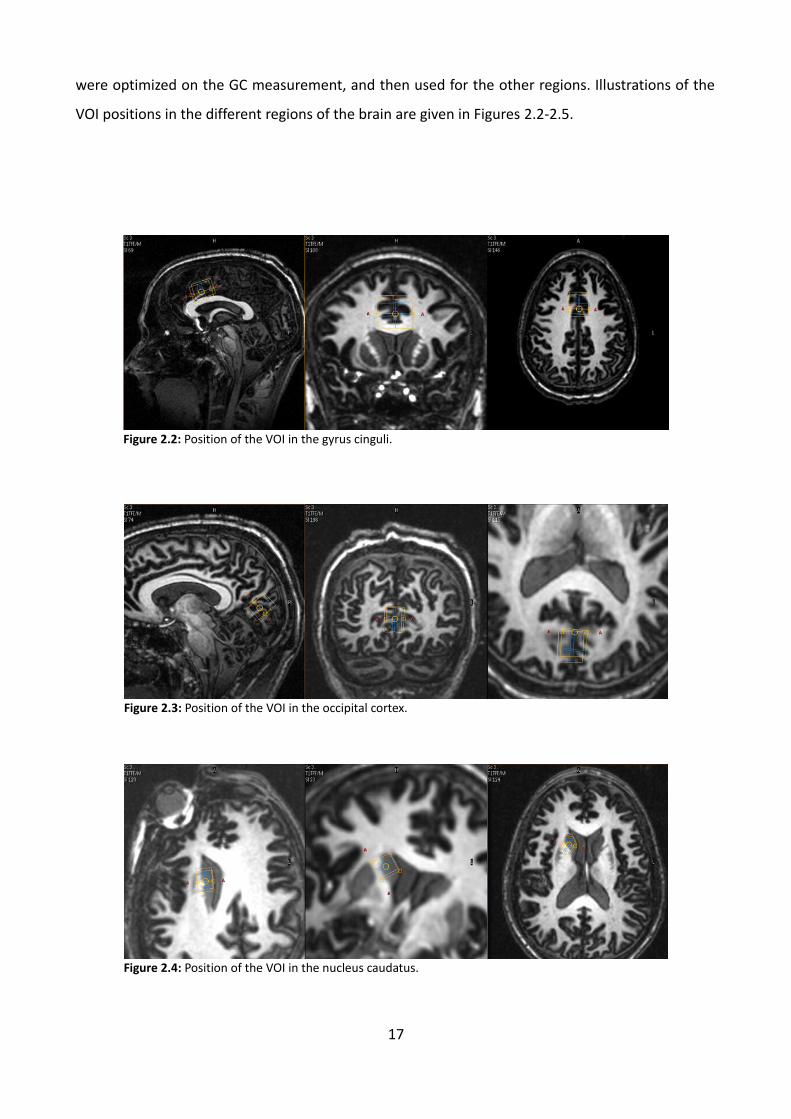
were optimized on the GC measurement, and then used for the other regions. Illustrations of the

VOI positions in the different regions of the brain are given in Figures 2.2-2.5.

17

Figure 2.2: Position of the VOI in the gyrus cinguli.

Figure 2.4: Position of the VOI in the nucleus caudatus.

Figure 2.3: Position of the VOI in the occipital cortex.

The volunteer gave written informed consent before any measurements were done.

The data from the in vivo measurements were analyzed in LCModel with the simulated basis set for

TE = 30 ms, with the same RF-pulse timing as that on the 3T system in use. The water

concentration cw, in mol/liter (M) in the regions were the VOIs were placed, was assumed to be

35880 mM according to LCModel recommendations[13]. A signal loss of 30 % from water due to

relaxation effects was assumed, also suggested by LCModel.

18

Figure 2.5: Position of VOI in the orbito frontal cortex.

3 RESULTS

3.1 Model spectra simulations

Figure 3.1 shows simulated PRESS spectra each for glutamate and creatine with TE = 30 ms, where

the timing of the RF-pulses of the sequence differ. Also shown is the difference between the

spectra. One can see a RF-pulse timing dependence in the glutamate spectra, but the creatine

simulation remained unaffected.

19

Figure 3.1: Simulated spectra from glutamate (A and B) and creatine (D and E) for TE = 30 ms, with different timing of the RF-pulses in the PRESS sequence, and the difference between them (C and F). In A and D the time between the 90o-pulse and the first and second 180o-pulse are 7.5000 and 22.5000 ms respectively. In B and E, the corresponding times are 9.1348 and 24.1348 ms, which is the implemented timing on the 3T system in use. C shows B – A and F shows E – D. Note the scale of the y-axis in C and F.

Simulated PRESS spectra for glutamate with TE = 30, 35, 40, 45, 144 and 288 ms are shown in

Figure 3.2. There is a complex TE dependence of the shape of the glutamate spectra. For creatine,

TE will only effect the amplitude of the peaks due to relaxation effects.

20

Figure 3.2: Simulated PRESS spectra from glutamate for TE = 30,35, 40, 45, 144 and 288 ms. One area, where the difference in the shape between the spectra is particularly visible, has been marked.

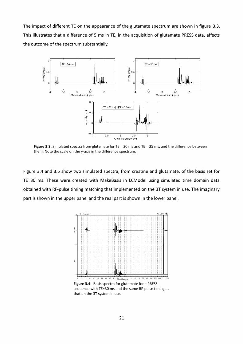
The impact of different TE on the appearance of the glutamate spectrum are shown in figure 3.3.

This illustrates that a difference of 5 ms in TE, in the acquisition of glutamate PRESS data, affects

the outcome of the spectrum substantially.

Figure 3.4 and 3.5 show two simulated spectra, from creatine and glutamate, of the basis set for

TE=30 ms. These were created with MakeBasis in LCModel using simulated time domain data

obtained with RF-pulse timing matching that implemented on the 3T system in use. The imaginary

part is shown in the upper panel and the real part is shown in the lower panel.

21

Figure 3.4: Basis spectra for glutamate for a PRESS sequence with TE=30 ms and the same RF-pulse timing as that on the 3T system in use.

Figure 3.3: Simulated spectra from glutamate for TE = 30 ms and TE = 35 ms, and the difference between them. Note the scale on the y-axis in the difference spectrum.

For a B0-field strength of 3T a FWHM of 0.2 Hz corresponds to 0.0016 ppm, which indicates that

the resolution demands from LCModel on the basis spectra, FWHM < 0.03 ppm, as mentioned in

Section 1.3, were well met.

3.2 Phantom measurements

Figure 3.6 shows a center slice phase image of the phantom. The B0-field homogeneity over the

phantom was found to be very good, exceeding by far that found in vivo.

22

Figure 3.5: Basis spectra for creatine for a PRESS sequence with TE=30 ms and the same RF-pulse timing as that on the 3T system in use.

Figure 3.6: A center slice phase image of the phantom. The image was acquired with TE = 64 ms, resulting in 0.12 ppm per phase wrap.

The phantom measurements with differing RF-pulse shapes for TE = 45 ms, yielded spectra with

differing shapes for glutamate. This can be seen in Figure 3.7.

Figure 3.8 and 3.9 show the results of the LCModel analysis of the data from the phantom

measurements of creatine and glutamate, acquired with TE = 30 ms, using the corresponding

simulated basis set, i.e. same TE and RF pulse timing as during the measurements.

23

Figure 3.8: The results from an LCModel analysis of the data from the phantom measurement of creatine, acquired with TE = 30 ms. The simulated basis set for TE = 30 ms, with the same RF pulse timing as on the 3T system in use, was used.

Figure 3.7: Spectrum from glutamate phantom measurement for TE = 45 ms. Spectrum A and B were acquired with the RF-pulse shape denoted Normal and Sharp respectively. The spectra are not to scale.

Non-random residuals in the fit were present in all measurements, indicating that the simulated

spectra do not account for all influences on the measured data. LCModel found that the best fit for

the measured creatine data was with the phosphocreatine spectrum in the basis set.

The FWHM of the single peaks in the measured spectra were in the range of 1-3 Hz, which

corresponds to 0.008-0.02 ppm.

24

Figure 3.9: The results from an LCModel analysis of the data from the phantom measurement of glutamate, acquired with TE = 30 ms. The simulated basis set for TE = 30 ms, with the same RF pulse timing as on the 3T system in use, was used.

3.3 Concentration calibration

The estimated concentrations with standard deviation, given by LCModel analysis of the data from

the phantom measurements, using corresponding basis sets, are shown in table 3.1.

Table 3.1: Results from the LCModel analysis of the data from the phantom measurements. The subscript of TE = 45 ms denotes the RF-pulse shape used for the measurement.

Glutamate Phoshpocreatine

TE (ms) Concentration (mM) SD (%) TE (ms) Concentration (mM) SD (%)

30 56.21 1 30 57.48 1

35 58.16 1 35 55.40 1

40 69.60 3 40 58.28 1

45normal 56.27 2 45normal 59.89 1

45sharp 55.36 3 45sharp 57.20 1

144 33.36 2 144 57.77 1

288 31.10 2 288 57.52 1

Since the concentration measurements for glutamate varied largely for the different TE:s, only the

results from the creatine data was considered in the concentration calibration. For consistency, the

concentration given for the measurement with the RF-pulse shape denoted Sharp was not

accounted for. Clcm and f in equation 2.1 was found to be 57.723 mM ± 2.5 % and 0.87 ± 2.5 %

respectively.

3.4 In vivo measurements

Figure 3.10-3.13 show the results of the LCModel analysis of the data from the in vivo

measurements, using the simulated basis set for TE = 30 and the same RF pulse timing as on the 3T

system in use. In Figure 3.10 is the spectrum from the gyrus cinguli measurement, in Figure 3.11 is

the nucleus caudatus spectrum, in Figure 3.12 is the occipital cortex spectrum and the spectrum

from the orbito frontal cortex is shown in Figure 3.13. Some structure can be seen in the residual in

the nucleus caudatus spectrum in the range 3.6 – 3.2 ppm, and in the occipital frontal cortex

spectrum in the range 4-3.8 ppm.

25

26

Figure 3.10: In vivo data from the gyrus cinguli analysed in LCModel with the simulated basis set for TE=30ms.

Figure 3.11: In vivo data from the nucleus caudatus, analyzed in LCModel with the simulated basis set for TE=30ms.

27

Figure 3.12: In vivo data from the occipital cortex, analyzed in LCModel with the simulated basis set for TE=30ms.

Figure 3.13: In vivo data from the orbito frontal cortex, analyzed in LCModel with the simulated basis set for TE=30ms.

4 DISCUSSION

Vespa-Simulation allows the user to design MRS pulse sequences and define metabolites in a

relatively straightforward way, making it very suitable for this work. One favorable quality in

particular of the software is the ability of giving the simulated time domain data as a textfile that is

directly readable for MakeBasis in LCModel.

Figure 3.1 shows that the timing of the RF-pulses in a PRESS sequence, influences the outcome of

the glutamate spectrum but has no effect on the spectrum from creatine, i.e. glutamate seems to

have a timing dependent signal modulation. This effect has been shown previously for glutamate

and other so called strongly coupled spin systems, where the J-coupling constant between spins is

in the same order of magnitude as the difference in chemical shift between them[19]. Therefor, in

order to achieve the best possible simulated basis set, the timing of the RF-pulses must be taken

into account for all coupled spins. However, the results also indicate that for the uncoupled spins

of acetate, choline, creatine, phosphocreatine, N-acetylaspartate, N-acetylaspartylglutamate and

scyllo-inositol, it is sufficient to create one basis set for each TE, which can be used for any RF-

pulse timing.

One demand on LCModel basis sets is that they are acquired with the same TE, to within a few ms,

of that used during acquisition of data. A visual comparison of the glutamate spectra in Figure 3.2

indicates that a significant difference in shape between spectra acquired with TE:s differing more

than 10 ms is present. Figure 3.3 shows that even a difference of 5 ms in TE results in prominent

differences. This is due to the TE dependent phase modulation of coupled spins, and illustrates the

need for as similar TE:s as possible between the measured data and the basis set, preferably

identical. As with the RF-pulse timing, the effect of different TE is not as severe on uncoupled

spins. The only visible effect will be a reduction in the area under the peaks in the spectrum due to

relaxation effects.

28

Difference in chemical shift between the two peaks of creatine and phosphocreatine, at about 3.2

and 3.9 ppm, are 0.002 and 0.02 ppm, see table 2.1, making it difficult to distinguish them from

one another in a MR spectrum. In analysis of in vivo MRS measurements with LCModel the sum of

the peaks from creatine and phoshocreatine is estimated, increasing the accuracy substantially as

compared to estimating each peak for itself[3].

There was a discrepancy between the simulated and in vitro measured spectra and the reason for

this can be several different experimental influences e.g. RF pulse shapes or Eddy currents. The

ideal hard RF-pulses used in the simulations is a simplified view of the reality. RF-pulses on MR

systems act on spins during a finite time, and will cause a variation of the flipangle over the object.

A phase variation of spins over the object can cause signal cancellation, which in turn might affect

the amplitudes in the final spectrum from an MRS measurement[20]. These effects are not taken

into account in these simulated spectra, which to some extent, might explain the discrepancies

between the measured and simulated data, see Figures 3.8 and 3.9. The possibility in Vespa-

Simulation to incorporate real RF-pulses in the simulation was considered, but was not feasible to

implement during this thesis, due to several practicalities. The difference between the spectra

measured with TE = 45 ms, as seen in Figure 3.7, could be due to the differing RF-pulse shapes

during the measurements. It is however difficult to determine to what extent, since the RF-pulse

timing in the two measurements also differ.

LCModel employes an Eddy current correction method which assumes negligible signal

components from the metabolites in the unsuppressed water signal[9], explained in Section 1.1.

This is a reasonable assumption for in vivo measurements, but in the phantom used in this work

the metabolite concentrations are much higher than those found in vivo. There is a possibility that

this might degrade the Eddy current correction, and contribute to the residual between the

phantom measurement data and the simulated spectra.

29

Although the FWHM of the basis set is smaller than that found of the single peaks in the data from

the phantom measurements, LCModel might not be optimal for finding a fit to this kind of data.

Phantom measurements yield much better resolution than in in vivo data, which is more forgiving.

A line broadening of the phantom data before analysis might give a better fit between the

simulated model spectra and the measured data. However, this would undermine the purpose of

the measurements, which was to verify that the simulations handled the more complex shape of

the measured spectra.

A satisfying explanation as to why the concentration of the glutamate phantom data given by

LCModel depends on the TE (Table 3.1) has not been found, however it could be linked to the

obtained residual of the fit. Relaxation effects on the metabolite in the phantom might also be a

contributing factor, but does not, according to the results for TE = 144 and 288 ms, exclusively

explain the effect.

By visual evaluation, the simulated basis set for TE = 30 ms seem to work very well on the in vivo

data. Figures 3.10-3.13 show residuals mainly consisting of noise. The structure present in the

residual of the nucleus caudatus and occipital frontal cortex spectra might be a consequence of the

residuals seen in the in vitro data analysis. Another very likely source of these non-random

residuals seen in vivo is that unwanted echos, originating from regions outside the VOI with

unsuppressed water, have disturbed the measurements. This effect, called the spurious echo

artifact, has previously been shown to give similar residuals of fitted data as that seen in this

work[21].

It is important to keep in mind that the metabolite concentrations given by LCModel, which are

scaled with reference to water, are not the actual concentrations present in the VOI. They will be

off by an unknown factor due to errors in the assumed water concentration and relaxation effects

on the water in the VOI, as mentioned above. Another factor affecting the outcome of the

LCModel analysis using the simulated basis set, is that relaxation effects on the metabolites are not

taken into account in the simulations. This might cause an underestimation of metabolite

concentrations, especially for long TE:s. However, in the course of one study, if all measurement

30

parameters are kept constant and if one expects that relaxation effects will not change

considerably from one measurement to another, the concentrations might still be used, with

arbitrary units, to observe concentration trends related to a pathological state. An alternative

common method is to use the LCModel concentrations given only in ratios relative to another

present metabolite. This method is only reliable if the concentration of the reference metabolite is

unaffected by any pathological state.

It is of great interest to set up a simulation environment for the creation of model spectra for

LCModel, since time and resources can be saved compared to measuring the model spectra from

phantom solutions. One advantage of measuring the model spectra in vitro is that many

experimental influences are automatically taken into account. In the creation of the simulated

model spectra as many of these influences as possible should be considered. Therefor, a natural

next step in improving the basis sets created in this work would be to implement the actual RF-

pulse shapes in the simulations.

31

5 CONCLUSION

LCModel basis sets was succesfully created for a PRESS sequence on a 3T MR system by simulation

with the software tool Vespa-Simulation. Spectra were simulated for six different TE:s and with

ideal “hard” RF-pulses with implemented RF pulse timing.

MRS measurements were performed on a phantom with known concentrations of glutamate and

creatine. The LCModel fit of the simulated basis set to the phantom measurement data resulted in

non-random residuals. This might be due to effects on the measured data originating from the

actual RF-pulse shapes on the MR system, not accounted for in the simulations. Concentrations

given by LCModel using the simulated basis sets needed to be corrected with a factor of 0.87 ±

2.5%.

In vivo MRS measurements were performed on a healthy volunteer in four different regions of the

brain. LCModel analysis of the data, using the simulated basis sets, showed good results for the fit.

Some structure in the residual could be seen in two of the fitted data sets, presumably a spurious

echo artifact or a consequence of the residuals seen in the fit of the phantom data.

32

Acknowledgments

A spectrum of people have helped we with this thesis, and to that I am very grateful. Firstly I would

like to thank my supervisors Maria Ljungberg and Åsa Carlsson for taking the time to provide

excellent guidance and feedback during this work. A special thanks to the creators of Vespa-

Simulation for letting me take part of their efforts. Marianne Wallgren at Klinisk Kemi at

Sahlgrenska University Hospital deserves a big thank you for the help with preparing the phantom

solutions. I would also like to thank the MR physicists, to whom I have been able to come to with

questions.

I want to thank my fellow students for making the last five years very special, I wish you all good

luck in your future endeavors! To my family, thank you for all the great support and

encouragement.

33

References1. Sibtain NA, Howe FA, Saunders DE. The clinical value of proton magnetic resonance

spectroscopy in adult brain tumours. Clin Radiol 2007;62(2):109-119.

2. Kantarci K. 1H magnetic resonance spectroscopy in dementia. Br J Radiol 2007;80(2):146-152.

3. Provencher SW. Estimation of metabolite concentrations from localized in vivo proton NMR Spectra. Magn Reson Med 1993;30(6):672-679.

4. McRobbie DW, Moore EA, Graves MJ, Prince MR. It's not just squiggles: in vivo spectroscopy. In: MRI. From picture to proton. 2nd ed. New York, USA: Cambridge University Press, 2007; 306-324.

5. deGraaf RA. Basic Principles. In: In vivo NMR spectroscopy. Principles and Techniques. 2nd ed. New York, USA: John Wiley and Sons , 2002; 1-40.

6. de Certaines JD, Bovée WMMJ, Podo F. 1D spectrum analysis. In: Magnetic resonance spectroscopy in biology and medicine. Functional and pathological tissue characterization. First ed. New York, USA: Pregamon Press, 1992; 31-58.

7. Bottomley PA. Spatial localization in NMR spectroscopy in vivo. Ann N Y Acad Sci 1987;508:333-348.

8. Haase A, Frahm J, Hanicke W, Matthaei D. 1H NMR chemical shift selective (CHESS) imaging. Phys Med Biol ;30(4):341-344.

9. Klose U. In vivo proton spectroscopy in presence of eddy currents. Magn Reson Med 1990;14(1):26-30.

10. Vespa-Simulation Web Site. http://scion.duhs.duke.edu/vespa/simulation.

11. Soher BJ, Semanchuk P, Young K, Todd, D. VeSPA - Simulation. User manual and reference. http://scion.duhs.duke.edu/vespa/simulation, March 9, 2011.

12. Smith SA, Levante TO, Meier BH, Ernst RR. Computer simulations in magnetic resonance. An object-oriented programming approach. J Magn Reson A 1993;106(1):75-105.

13. Provencher SW. LCModel & LCMgui user's manual. LCModel Web Site. http://s-provencher.com/pages/lcm-manual.shtml, March 18, 2011.

14. Gamma performance Vs. Spin Count. Vespa Web Site. http://scion.duhs.duke.edu/vespa/gamma/wiki/GammaVsSpin .

34

15. PyGAMMA vs GAMMA.Vespa Web Site. http://scion.duhs.duke.edu/vespa/gamma/wiki/GammaVsPyGamma.

16. Govindaraju V, Young K, Maudsley AA. Proton NMR chemical shifts and coupling constants for brain metabolites. NMR Biomed 2000;13(3):129-153.

17. Ljungberg M, Bengtsson F, Carlsson Å, Lagerstrand K, Starck G, Vikhoff-Baaz B, Forssell-Aronsson E. A phantom design that minimizes the magnetic field inhomogeneity. European Society for Magnetic Resonance in Medicine and Biology ’22 2005, Basel, #503.

18 Bengtsson F. Creation of high quality sets of in vitro model spectra for Philips Gyroscan Intera 1.5 T for improved analysis of 1H in vivo MR spectra with LCModel, 2004, Dept. of Radiation Physics , Gothenburg University.

19. Snyder J, Wilman A. Field strength dependence of PRESS timings for simultaneous detection of glutamateand glutamine from 1.5 to 7 T. J Magn Reson 2010;203(1):66-72.

20. Ernst TH, Henning J. Coupling effects in volume selective 1H spectroscopy of major brain metabolites. Magn Reson Med 1991;21(1):82-96.

21. Slotboom J, Mehlkopf AF, Bovée WMMJ. The effects of frequency selective RF-pulses on J-coupled spin-1/2 systems. J Magn Reson A 1994;108(1):38-50.

22. Starck G, Carlsson Å, Ljungberg M, Forsell-Aronsson E. k-space analysis of point-resolved spectroscopy (PRESS) with regard to spurious echos in in vivo 1H MRS. NMR Biomed 2008;22(2):137-147.

35