simulation optimization: new advances for real world optimization fred glover marco better
Post on 22-Dec-2015
221 views
TRANSCRIPT

SIMULATION OPTIMIZATION: NEW ADVANCES FOR REAL
WORLD OPTIMIZATION
Fred Glover
Marco Better

Slide 3
What is Simulation Optimization?
The optimization of simulation models deals with the situation in which the analyst would like to find which of possibly many sets of model specifications (i.e., input parameters and/or structural assumptions) leads to optimal performance
Inputparameters
Measure of performance
Slide 4
Simulation OptimizationWhy is it required?
Complex models contain many variables and constraints as well as uncertainty
What-if simulation analysis unlikely to result in an optimal answer due to large number of possible solutions
Inability of pure optimization to model complexities, uncertainties and dynamics of scenarios.
Simulation-Optimization removes these inabilities by combining both approaches.
Slide 5
Simulation-OptimizationWhy is it required?
A total solution requires both capabilities.
Two-Step SolutionSimulationOptimization
Both are necessary, neither is sufficient.

Slide 6
Simulation OptimizationBenefits in Dealing with Uncertainty
Simulation enables understanding/modeling and communications of uncertainty.
Optimization enables management of uncertainty.
Slide 9
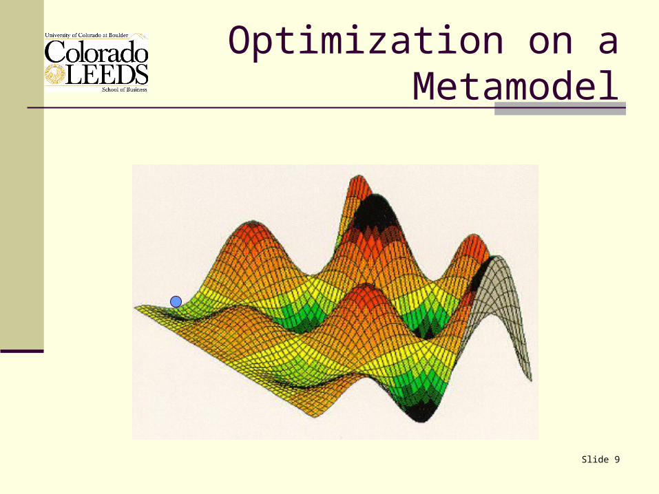
Optimization on a Metamodel
Slide 10
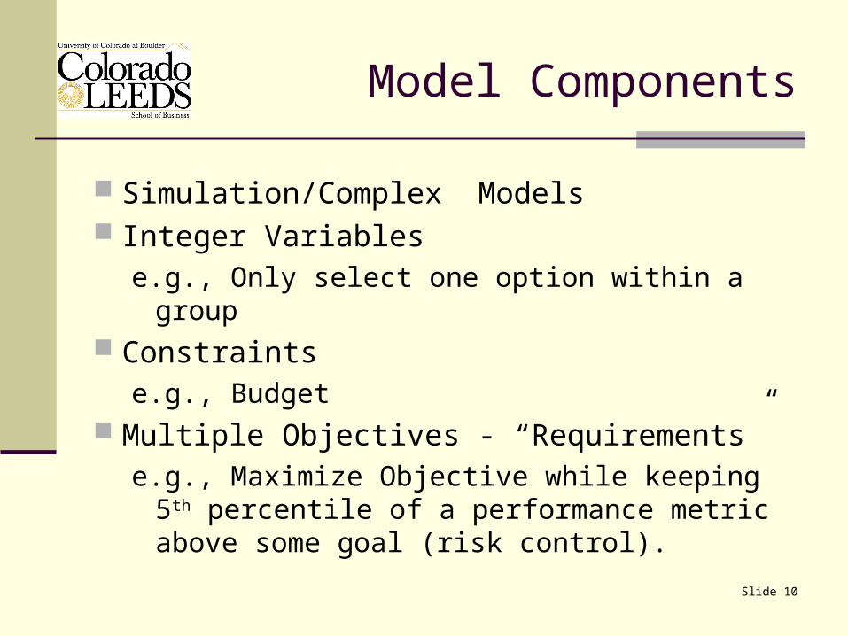
Model Components
Simulation/Complex Models Integer Variables
e.g., Only select one option within a group Constraints
e.g., Budget Multiple Objectives - “Requirements”
e.g., Maximize Objective while keeping 5th percentile of a performance metric above some goal (risk control).

Slide 11
Simulation Optimization
InputsSimulator / Complex System Outputs
OptQuest
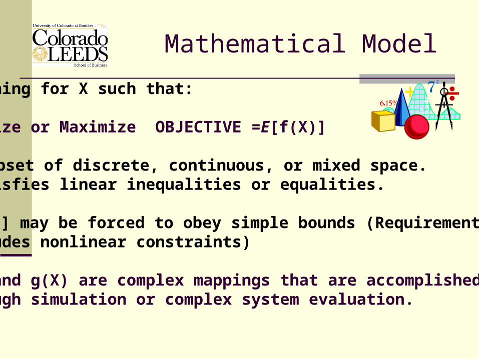
Mathematical Model
Searching for X such that:
Minimize or Maximize OBJECTIVE =E[f(X)]
XSubset of discrete, continuous, or mixed space.X satisfies linear inequalities or equalities.
E[g(X)] may be forced to obey simple bounds (Requirements)(includes nonlinear constraints)
f(X) and g(X) are complex mappings that are accomplished through simulation or complex system evaluation.

The Optimization Challenge
Function to be Optimized Highly Nonlinear Nondifferentiable Discrete or Continuous or Mixed
Function Evaluations Complex Extremely Computer Intensive One second to One Day per Evaluation!

Slide 14
OptQuest®
Scatter SearchAdvanced Tabu SearchLinear ProgrammingInteger ProgrammingNeural NetworksLinear Regression
Research funded by National Science Foundation and Office of Naval Research.
Slide 15
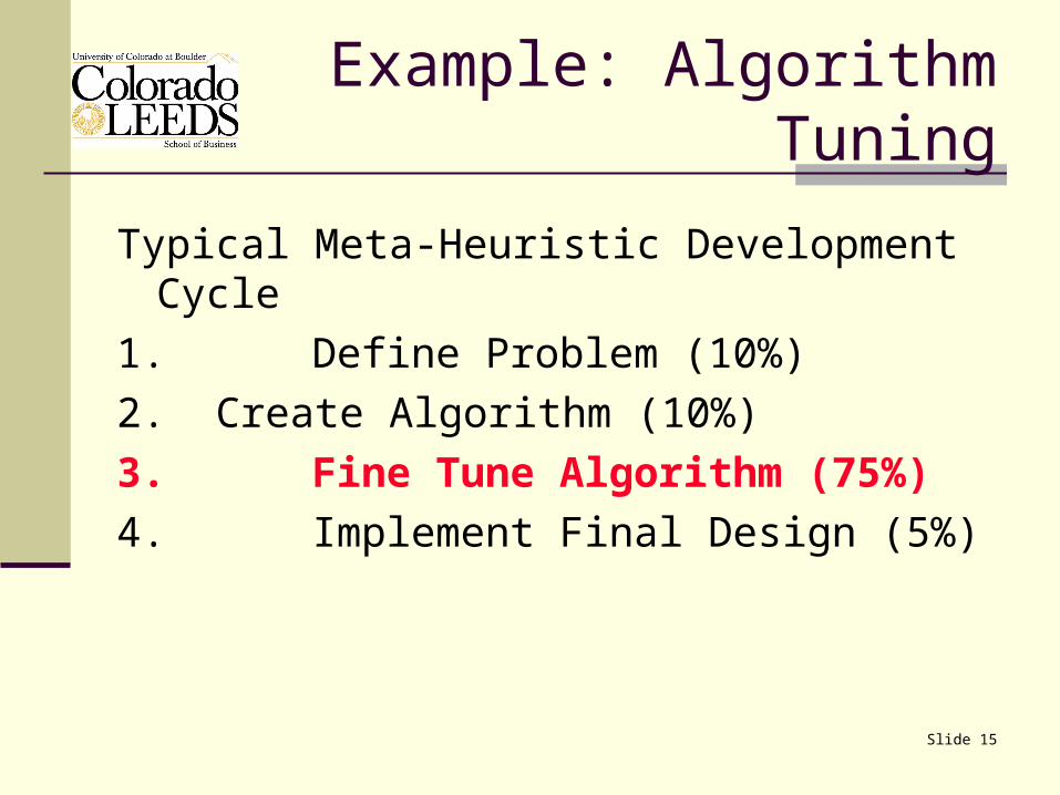
Example: Algorithm Tuning
Typical Meta-Heuristic Development Cycle
1. Define Problem (10%)
2. Create Algorithm (10%)
3. Fine Tune Algorithm (75%)
4. Implement Final Design (5%)

Algorithm Tuning with OptQuest
Tabu Searchfor Bandwidth
PackingAlgorithm*
Paths per CallFrequency PenaltyShort-Term MemoryMedium-Term MemoryLong-Term MemoryTenure
OptQuest
Profit
*Laguna & Glover, Management Science, 1993.
Slide 17
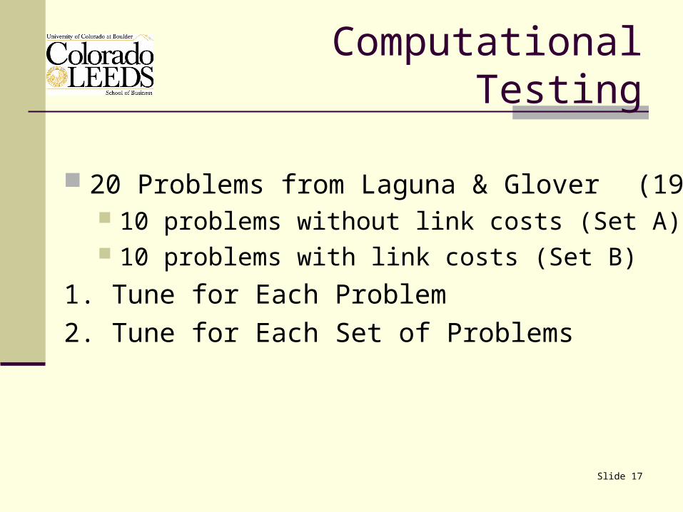
Computational Testing
20 Problems from Laguna & Glover (1993) 10 problems without link costs (Set A) 10 problems with link costs (Set B)
1. Tune for Each Problem
2. Tune for Each Set of Problems

Slide 18
Tuning per Problem Profits (Without Link Costs: Set A)
Laguna & Glover (1993) OptQuest7,540 7,754 +2,100 2,10013,550 13,710 +2,955 2,9552,345 2,395 +9,010 9,01011,000 11,160 +12,810 12,8105,780 5,780970 970
Slide 19
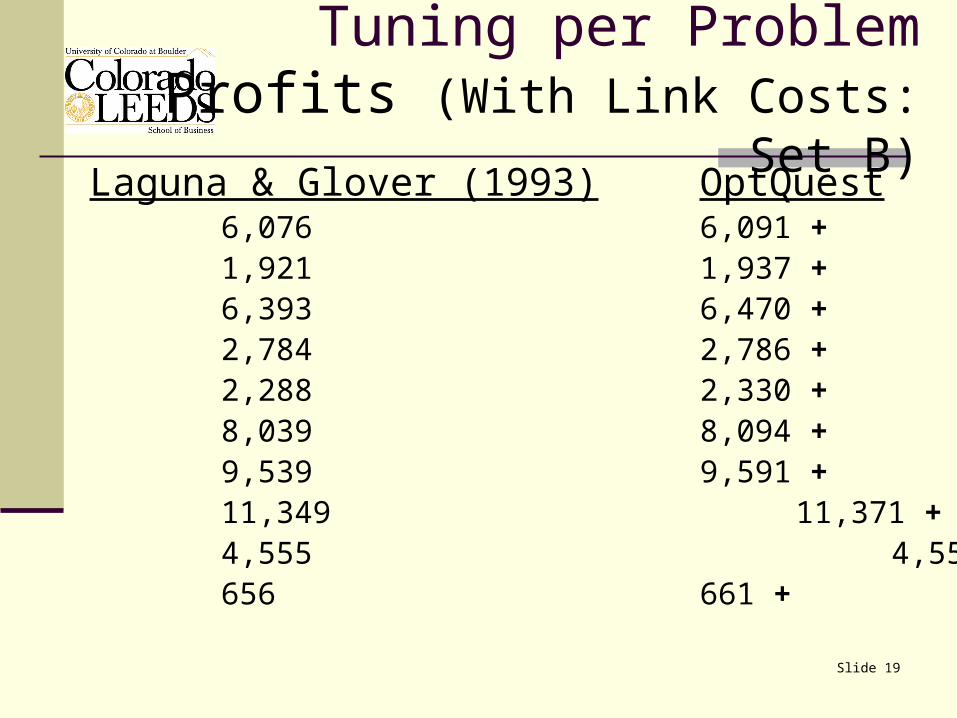
Tuning per ProblemProfits (With Link Costs: Set B)
Laguna & Glover (1993) OptQuest6,076 6,091 +1,921 1,937 +6,393 6,470 +2,784 2,786 +2,288 2,330 +8,039 8,094 +9,539 9,591 +11,349 11,371 +4,555 4,555656 661 +
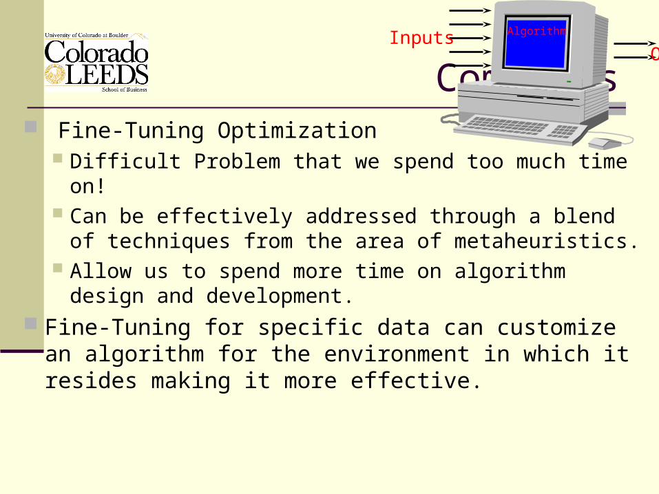
Comments Fine-Tuning Optimization
Difficult Problem that we spend too much time on! Can be effectively addressed through a blend of
techniques from the area of metaheuristics. Allow us to spend more time on algorithm design and
development. Fine-Tuning for specific data can customize an
algorithm for the environment in which it resides making it more effective.
AlgorithmInputsOutputs
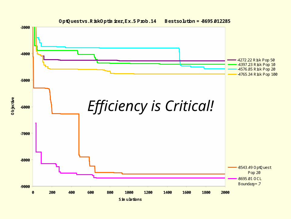
OptQuest vs. RiskOptimizer, Ex. 5 Prob. 14 Best solution = -8695.012285
-4397.23 Risk Pop 10-4576.85 Risk Pop 20
-4272.22 Risk Pop 50
-4765.34 Risk Pop 100
-8543.49 OptQuest Pop 20
-8695.01 OCL Boundary=.7
-9000
-8000
-7000
-6000
-5000
-4000
-3000
0 200 400 600 800 1000 1200 1400 1600 1800 2000
Simulations
Ob
ject
ive
Efficiency is Critical!

Slide 40
OptQuest®
Simulation Optimization Applications:
the best configuration of machines for production scheduling the best integration of manufacturing, inventory and distribution the best layouts, links and capacities for network design the best investment portfolio for financial planning the best utilization of employees for workforce planning the best location of facilities for commercial distribution the best operating schedule for electrical power planning the best assignment of medical personnel in hospital administration the best setting of tolerances in manufacturing design the best set of treatment policies in waste management

Slide 41
Selection of the Best Solution
Using a sample-path approach turns the evaluation into a deterministic process
If the evaluation is stochastic (i.e., no unique sample is used) then statistical significance is important for comparison purposes
Observed mean value of bestsolution
Observed meanvalue of candidatesolution
Slide 42
An Example of Simulation Applied to the Oil & Gas Industry
Slide 43
Problem
Given a set of opportunities and limited resources determine the best set of projects that maximize performance while controlling risk.
Create a new portfolio
Augment an existing portfolio
Slide 44
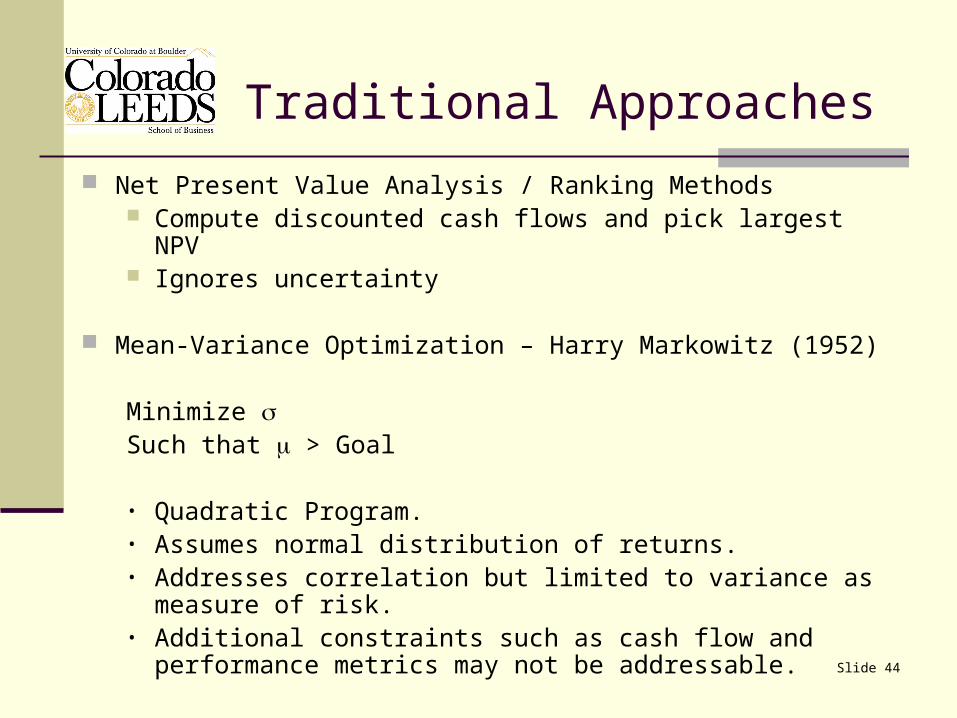
Traditional Approaches
Net Present Value Analysis / Ranking Methods Compute discounted cash flows and pick largest NPV Ignores uncertainty
Mean-Variance Optimization – Harry Markowitz (1952)
Minimize Such that > Goal
• Quadratic Program.• Assumes normal distribution of returns.• Addresses correlation but limited to variance as measure of
risk.• Additional constraints such as cash flow and performance
metrics may not be addressable.
Slide 45
Simulation-Based Portfolio Selection
Use Monte Carlo simulation to model projects. Unlimited ability to model complex situations. Risk can be defined multiple ways.
Use OptQuest to select projects. Objectives based on outputs from simulation. Additional constraints based on cash flows,
etc.
Slide 46
Components
Simulation Model Integer Variables
e.g., Only invest in one project within a group Constraints
e.g., Cash Flow, time, personnel Multiple Objectives - “Requirements”
e.g., Maximize Return Mean while keeping 5th percentile of return above some goal (risk control).

Slide 47
Application Information
5 Projects Tight Gas Play Scenario (TGP) Oil – Water Flood Prospect (OWF) Dependent Layer Gas Play Scenario (DL) Oil - Offshore Prospect (OOP) Oil - Horizontal Well Prospect (OHW)
Ten year models that incorporate multiple types of uncertainty

Slide 48
Budget-Constrained Project Selection
5 Projects Expected Revenue and Distribution Probability of Success Cost
$2,000,000 Budget
Slide 49
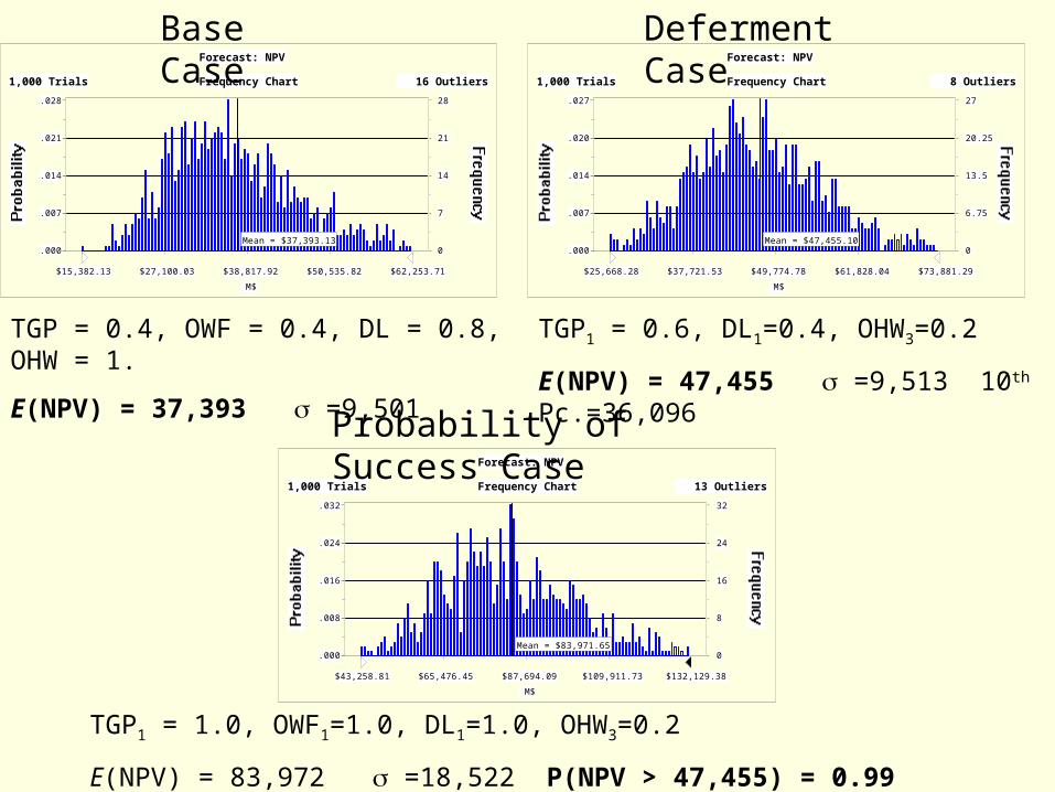
Base Case
Determine participation levels in each project [0,1] (Decision Variables) that
Maximize E(NPV) (Forecast) While keeping < 10,000 M$ (Forecast)
All projects must start in year 1.

Frequency Chart
M$
Mean = $37,393.13.000
.007
.014
.021
.028
0
7
14
21
28
$15,382.13 $27,100.03 $38,817.92 $50,535.82 $62,253.71
1,000 Trials 16 Outliers
Forecast: NPV
Base Case
TGP = 0.4, OWF = 0.4, DL = 0.8, OHW = 1.
E(NPV) = 37,393 =9,501

Slide 51
Deferment Case
Determine participation levels in each project [0,1] AND starting times for each project that
Maximize E(NPV) While keeping < 10,000 M$
All projects may start in year 1, year 2, or year 3. (5x3=15 Decision Variables)
Constraints?

Frequency Chart
M$
Mean = $37,393.13.000
.007
.014
.021
.028
0
7
14
21
28
$15,382.13 $27,100.03 $38,817.92 $50,535.82 $62,253.71
1,000 Trials 16 Outliers
Forecast: NPV
Base CaseFrequency Chart
M$
Mean = $47,455.10.000
.007
.014
.020
.027
0
6.75
13.5
20.25
27
$25,668.28 $37,721.53 $49,774.78 $61,828.04 $73,881.29
1,000 Trials 8 Outliers
Forecast: NPV
TGP1 = 0.6, DL1=0.4, OHW3=0.2
E(NPV) = 47,455 =9,513 10th Pc.=36,096
Deferment Case
TGP = 0.4, OWF = 0.4, DL = 0.8, OHW = 1.
E(NPV) = 37,393 =9,501

Slide 53
Probability of Success Case
Determine participation levels in each project [0,1] AND starting times for each project that
Maximize P(NPV > 47,455 M$) While keeping 10th Percentile of NPV > 36,096 M$
All projects may start in year 1, year 2, or year 3.
Frequency Chart
M$
Mean = $37,393.13.000
.007
.014
.021
.028
0
7
14
21
28
$15,382.13 $27,100.03 $38,817.92 $50,535.82 $62,253.71
1,000 Trials 16 Outliers
Forecast: NPV
Base CaseFrequency Chart
M$
Mean = $47,455.10.000
.007
.014
.020
.027
0
6.75
13.5
20.25
27
$25,668.28 $37,721.53 $49,774.78 $61,828.04 $73,881.29
1,000 Trials 8 Outliers
Forecast: NPV
TGP1 = 0.6, DL1=0.4, OHW3=0.2
E(NPV) = 47,455 =9,513 10th Pc.=36,096
Deferment Case
Frequency Chart
M$
Mean = $83,971.65.000
.008
.016
.024
.032
0
8
16
24
32
$43,258.81 $65,476.45 $87,694.09 $109,911.73 $132,129.38
1,000 Trials 13 Outliers
Forecast: NPV
TGP1 = 1.0, OWF1=1.0, DL1=1.0, OHW3=0.2
E(NPV) = 83,972 =18,522 P(NPV > 47,455) = 0.99 10th Pc.=53,359
Probability of Success Case
TGP = 0.4, OWF = 0.4, DL = 0.8, OHW = 1.
E(NPV) = 37,393 =9,501
Slide 55
Benefits
Easy to use Quickly evaluate many planning alternatives Optimized financial performance Better risk control using familiar metrics

Slide 56
Results for IT Capital Budgeting in a Large Energy Company
Slide 57
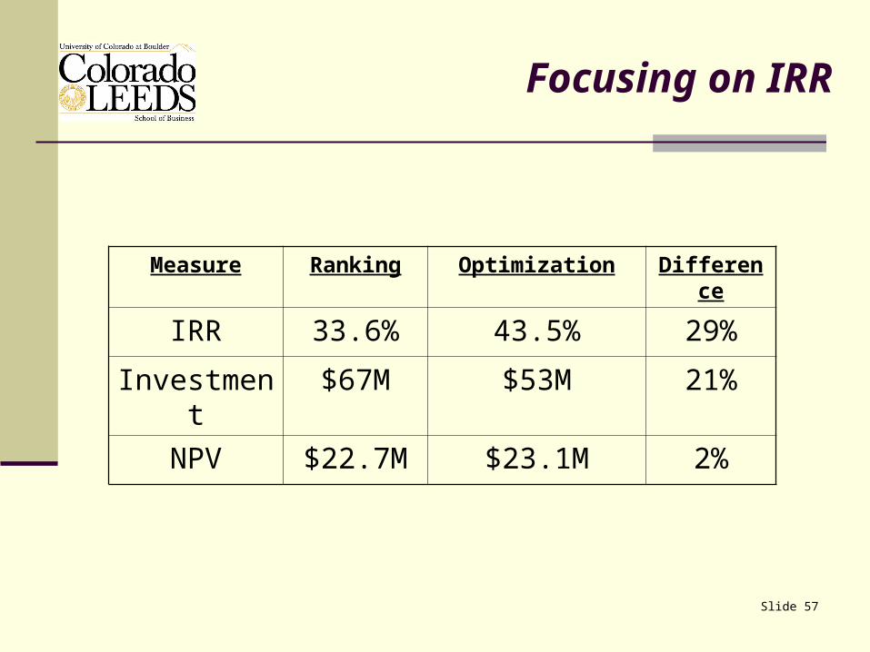
Focusing on IRR
Measure Ranking Optimization Difference
IRR 33.6% 43.5% 29%
Investment $67M $53M 21%
NPV $22.7M $23.1M 2%
Slide 58
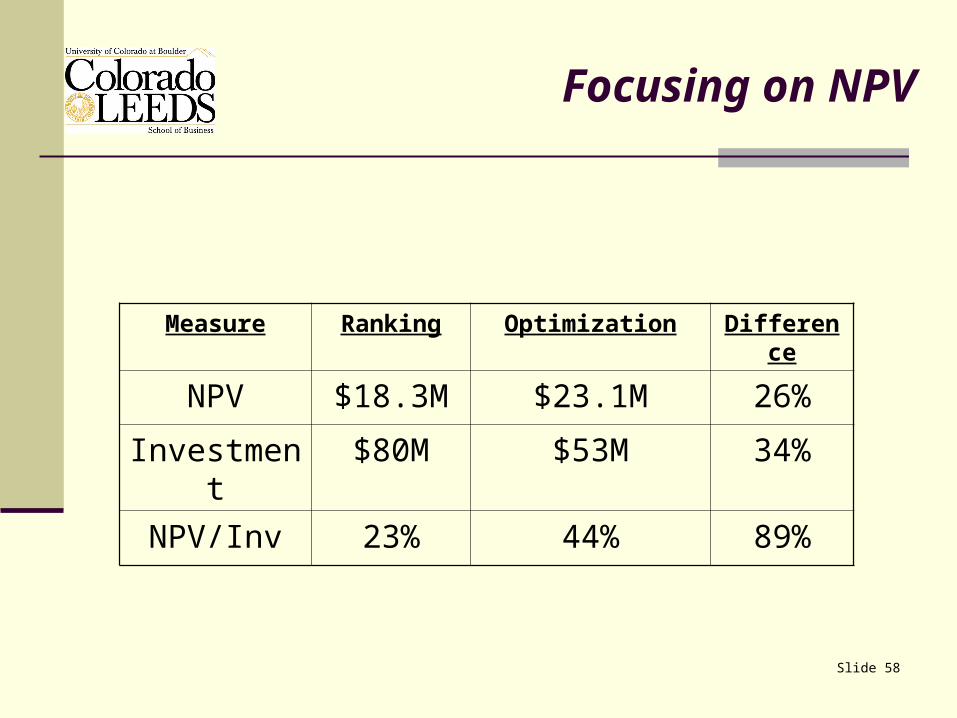
Focusing on NPV
Measure Ranking Optimization Difference
NPV $18.3M $23.1M 26%
Investment $80M $53M 34%
NPV/Inv 23% 44% 89%
Slide 59
Software Demonstrations
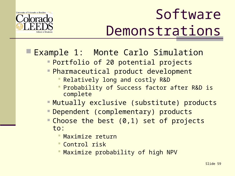
Example 1: Monte Carlo Simulation Portfolio of 20 potential projects Pharmaceutical product development
Relatively long and costly R&D Probability of Success factor after R&D is complete
Mutually exclusive (substitute) products Dependent (complementary) products Choose the best (0,1) set of projects to:
Maximize return Control risk Maximize probability of high NPV
Slide 60
Software Demonstrations
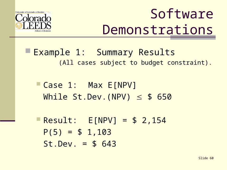
Example 1: Summary Results(All cases subject to budget constraint).
Case 1: Max E[NPV]
While St.Dev.(NPV) $ 650
Result: E[NPV] = $ 2,154
P(5) = $ 1,103
St.Dev. = $ 643

Slide 61
Software Demonstrations
Example 1: Summary Results(All cases subject to budget constraint).
Case 2: Max E[NPV]
While P(5) $ 1,103
Result: E[NPV] = $ 2,346
P(5) = $ 1,159
St.Dev. = $ 725

Slide 62
Software Demonstrations
Example 1: Summary Results(All cases subject to budget constraint).
Case 3: Max P(NPV > $2,154)
Result: P(NPV > $2,154) = 62%
E[NPV] = $ 2,346
P(5) = $ 1,159
St.Dev. = $ 725

Slide 63
Software Demonstrations
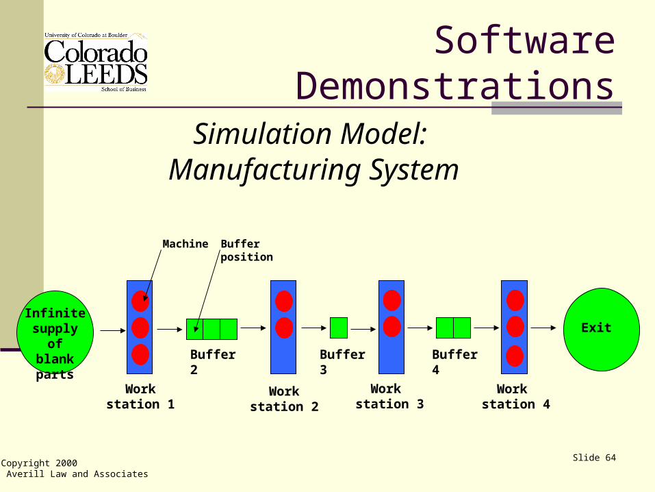
Example 2: Discrete Event Simulation Job Shop Design 4 workstations and 3 buffer zones for WIP Choose the number of machines in each
workstation (1,3) and the number of slots in each buffer (1,10) in order to:
Maximize throughput Maximize profit
Slide 64
Software Demonstrations
Simulation Model: Manufacturing System
Buffer 2 Buffer 3 Buffer 4
Work station 2
Work station 3
Machine Buffer position
Infinitesupply of
blank parts
Exit
Copyright 2000 Averill Law and Associates
Work station 1
Work station 4
Slide 65
Software Demonstrations
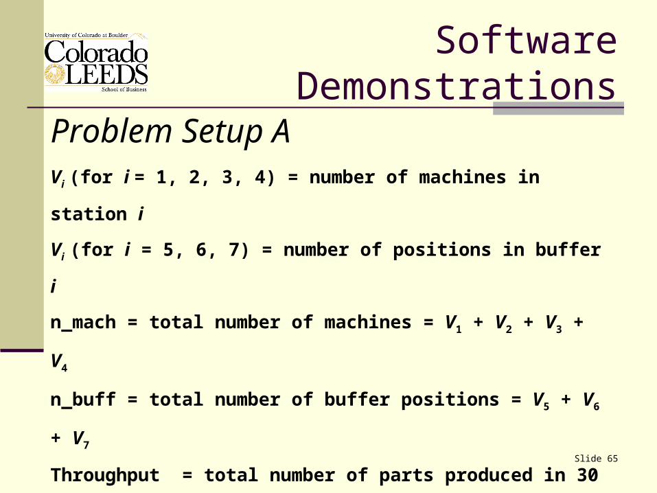
Problem Setup AVi (for i = 1, 2, 3, 4) = number of machines in station i
Vi (for i = 5, 6, 7) = number of positions in buffer i
n_mach = total number of machines = V1 + V2 + V3 + V4
n_buff = total number of buffer positions = V5 + V6 + V7
Throughput = total number of parts produced in 30 days
Objective Function (Response): Maximize Profit
Profit = ($200 * Throughput) - ($25,000 * n_mach) - ($1,000 * n_buff)
Bounds for Controls
1 ≤ Vi (for i = 1, 2, 3, 4) ≤ 3 1 ≤ Vi (for i = 5, 6, 7) ≤ 10
Slide 66
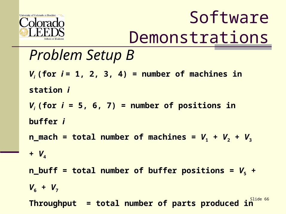
Software Demonstrations
Problem Setup BVi (for i = 1, 2, 3, 4) = number of machines in station i
Vi (for i = 5, 6, 7) = number of positions in buffer i
n_mach = total number of machines = V1 + V2 + V3 + V4
n_buff = total number of buffer positions = V5 + V6 + V7
Throughput = total number of parts produced in 30 days
Objective Function (Response): Maximize ThroughputBounds for Controls1 ≤ Vi (for i = 1, 2, 3, 4) ≤ 3 1 ≤ Vi (for i = 5, 6, 7) ≤ 10
Cost Constraint on Controls
25000*(n_mach) + 1000*(n_buff) ≤ 235000

Slide 67
Conclusions
There is still much to learn and discover about how to optimize simulated systems both from
the theoretical and the practical points of view.
The opportunities are exciting!

Slide 68
Questions & Feedback
www.OptTek.com
(303) 447-3255
[email protected] - [email protected] - Jim