simulation problem analysis and research kernel · visualspark 2.0 users guide 1 introduction spark...
TRANSCRIPT

VISUALSPARK 2.0
USERS GUIDE
Simulation Problem Analysis and Research Kernel
Copyright 1997-2003 Lawrence Berkeley National Laboratory
Ayres Sowell Associates, Inc. Pending approval of the U.S. Department of Energy. All rights reserved.
This work was supported by the Assistant Secretary for Energy Efficiency and Renewable Energy, Office of Building Technologies Program of the
U.S. Dept. of Energy. Contract No. DE-AC03-76SF00098.
VisualSPARK 2.0 Users Guide
TABLE OF CONTENTS
TABLE OF CONTENTS ................................................................................................................................................. I
FOREWORD ................................................................................................................................................................. III
TEXT CONVENTIONS ............................................................................................................................................... IV
1 INTRODUCTION ...................................................................................................................................................5 1.1 AVAILABILITY AND LICENSING..........................................................................................................................5 1.2 DOCUMENTATION ..............................................................................................................................................5 1.3 HELP ..................................................................................................................................................................5 1.4 NAMING CONVENTION.......................................................................................................................................6
2 UNIX VERSIONS: DOWNLOADING AND INSTALLATION INSTRUCTIONS FOR RED HAT LINUX 8.0 (INTEL PROCESSORS) ...........................................................................................................................................7
2.1 REGISTRATION...................................................................................................................................................7 2.2 OTHER SOFTWARE REQUIRED............................................................................................................................7 2.3 INSTALL VISUALSPARK ...................................................................................................................................7 2.4 UNINSTALL VISUALSPARK ................................................................................................................................8
3 WINDOWS VERSIONS: DOWNLOADING AND INSTALLATION INSTRUCTIONS FOR WINDOWS 95/98/ME/NT/2000............................................................................................................................................................9
3.1 REGISTRATION...................................................................................................................................................9 3.2 OTHER SOFTWARE REQUIRED............................................................................................................................9 3.3 INSTALL VISUALSPARK ...................................................................................................................................9 3.4 UNINSTALL VISUALSPARK ................................................................................................................................9 3.5 SPECIFY TARGET C++ COMPILER .....................................................................................................................9
4 VISUALSPARK ENVIRONMENT SETTINGS ................................................................................................11 4.1 ENVIRONMENT VARIABLES..............................................................................................................................11 4.1.1 SPARK_DIR ..........................................................................................................................................11 4.1.2 PATH ......................................................................................................................................................11 4.1.3 SPARK_PDFVIEWER ............................................................................................................................11 4.1.4 SPARK_HTMVIEWER ............................................................................................................................12 4.1.5 SPARK_CHMVIEWER...............................................................................................................................12
4.2 ENVIRONMENT FILES .......................................................................................................................................12 4.2.1 classpath.env...............................................................................................................................................12 4.2.2 projects.env.................................................................................................................................................12 4.2.3 sparkenv.sh or sparkenv.csh .....................................................................................................................13 4.2.4 sparkenv.bat .................................................................................................................................................13
5 COMMAND LINE EXECUTION OF SPARK ...................................................................................................14 5.1 THE SPARK DIRECTORY STRUCTURE..............................................................................................................14 5.2 COMMANDS .....................................................................................................................................................15 5.3 PREPARATIONS ................................................................................................................................................15 5.4 BUILD AND RUN...............................................................................................................................................16
5.4.1 Run-Control Information............................................................................................................................17 5.4.2 Results.........................................................................................................................................................17
i
5.4.3 The runspark Command .............................................................................................................................18

VisualSPARK 2.0 Users Guide
5.4.4 The runspark Flags.....................................................................................................................................18 5.4.5 Re-running a Problem Executable..............................................................................................................18
5.5 EXAMPLES .......................................................................................................................................................19 5.6 USING SPARK OUTPUT....................................................................................................................................20
6 USING THE GRAPHICAL USER INTERFACE (GUI)...................................................................................21 6.1 THE MAIN VISUALSPARK WINDOW.................................................................................................................21 6.2 THE PROJECT MENU ........................................................................................................................................26
6.2.1 Creating and Copying Projects ..................................................................................................................26 6.2.2 Make Package, Make Clean, Make CleanALL .........................................................................................27
6.3 NEW INPUT SET OR EDIT INPUT SET.................................................................................................................27 6.3.1 Input Editor.................................................................................................................................................28 6.3.2 Run-Time Parameters.................................................................................................................................29
6.4 RUNNING .........................................................................................................................................................30 6.4.1 The Run Command .....................................................................................................................................30 6.4.2 Log Files and Error Reports.......................................................................................................................31
6.5 COMPONENT PREFERENCES .............................................................................................................................31 6.5.1 “Defaults/Global/Structure” Tab...............................................................................................................31 6.5.2 The Components Tabs ................................................................................................................................32
6.6 VIEWING AND PLOTTING RESULTS...................................................................................................................33 6.6.1 View results file (as text).............................................................................................................................33 6.6.2 Dynamic, 1 Variable per Plot.....................................................................................................................33 6.6.3 Dynamic, multiple variables per plot .........................................................................................................34 6.6.4 Real-Time Dynamic Plot.............................................................................................................................35 6.6.5 Phase Plot...................................................................................................................................................36 6.6.6 Zooming In and Out....................................................................................................................................36 6.6.7 Plotting Results from Several Different Problems......................................................................................36
6.7 EDITING PROJECTS AND CLASSES ....................................................................................................................40 6.8 CREATING SPARK CLASSES ...........................................................................................................................41
7 TUTORIAL............................................................................................................................................................43 7.1 ROOM_FC EXAMPLE .........................................................................................................................................43
7.1.1 Getting Started............................................................................................................................................43 7.1.2 Running the Model......................................................................................................................................44 7.1.3 Viewing the Results.....................................................................................................................................45 7.1.4 Modifying the Values for the Input Variables.............................................................................................51
7.2 SUM5 EXAMPLE................................................................................................................................................54 7.2.1 Create a New Project..................................................................................................................................54 7.2.2 Create the Supporting Classes....................................................................................................................56 7.2.3 Create the Input Data .................................................................................................................................59
7.3 ROOM_PI EXAMPLE ..........................................................................................................................................60 7.3.1 Create the Project.......................................................................................................................................61 7.3.2 Create the Macro Class ac_pi and the Atomic Class pi_formula ..............................................................63 7.3.3 Create the Macro Class Room....................................................................................................................66 7.3.4 Create a New Input Set and Run the Problem............................................................................................68 7.3.5 Run Simulation and Plot the Results ..........................................................................................................72 7.3.6 Use Temperatures from EnergyPlus Weather Data File............................................................................72
8 SUPPORT...............................................................................................................................................................75
GLOSSARY OF TERMS ..............................................................................................................................................76
INDEX .............................................................................................................................................................................81
ii

VisualSPARK 2.0 Users Guide
FOREWORD
This guide is an introduction to using the VisualSPARK version of the SPARK program. It addresses platform-specific issues; provides installation instructions for Windows®, UNIX® and Linux® platforms; and presents a set of tutorials.
Before going through the tutorials you should read the sections of the SPARK Reference Manual about the basic methodology in order to familiarize yourself with the basic concepts that underlie the SPARK approach to setting up and solving simulation problems.
This work was supported by the Assistant Secretary for Energy Efficiency and Renewable Energy, Office of Building Technology, State and Community Programs, Office of Building Systems of the U.S. Department of Energy, under contract DE-AC03-76SF00098.
NOTICE: The Government is granted for itself and others acting on its behalf a paid-up, nonexclusive, irrevocable, worldwide license in this data to reproduce, prepare derivative works, and perform publicly and display publicly. Beginning five (5) years after (date permission to assert copyright was obtained) and subject to any subsequent five (5) year renewals, the Government is granted for itself and others acting on its behalf a paid-up, nonexclusive, irrevocable, worldwide license in this data to reproduce, prepare derivative works, distribute copies to the public, perform publicly and display publicly, and to permit others to do so. NEITHER THE UNITED STATES NOR THE UNITED STATES DEPARTMENT OF ENERGY, NOR ANY OF THEIR EMPLOYEES, MAKES ANY WARRANTY, EXPRESS OR IMPLIED, OR ASSUMES ANY LEGAL LIABILITY OR RESPONSIBILITY FOR THE ACCURACY, COMPLETENESS, OR USEFULNESS OF ANY INFORMATION, APPARATUS, PRODUCT, OR PROCESS DISCLOSED, OR REPRESENTS THAT ITS USE WOULD NOT INFRINGE PRIVATELY OWNED RIGHTS.
The SPARK simulation program is not sponsored by or affiliated with SPARC International, Inc. and is not based on SPARC architecture.
iii

VisualSPARK 2.0 Users Guide
TEXT CONVENTIONS
Throughout this manual, we use different typefaces as follows:
Program Name
File Name
KEYWORD Screen Display, Code, Key
User Entry <enter>
Button, Menu “Window”, “Dialog box”, “Panel”, “Tab”, “Label” In addition, when discussing SPARK terminology italic and bold typefaces identify the different entities, as follows: problem name macro class
object name atomic class
probe, link name port name
problem variable port variable
iv

VisualSPARK 2.0 Users Guide
1 INTRODUCTION SPARK is a general software program for solving simulation problems. It can be run on a variety of platforms. User interfaces for SPARK are considered to be separate software programs which, except for the built-in command-line interface, tend to be platform specific. SPARK targets two platforms, namely UNIX workstations and Intel-based platforms running Linux or Microsoft Windows 95, 98, NT or 2000. This document deals with a graphical user interface called VisualSPARK.
The SPARK Reference Manual provides overview, examples, and language reference that are, to the extent possible, platform independent. This document supplements the Reference Manual, giving installation and usage information for Windows and UNIX platforms, and describing how to use the VisualSPARK interface to set up and run simulation problems..
1.1 AVAILABILITY AND LICENSING Windows and UNIX versions of VisualSPARK are available after the execution of the Licensing Agreement. You can execute the Licensing Agreement by visiting the Simulation Research Group Web site at http://SimulationResearch.lbl.gov as discussed under Installation below.
Binary files that are part of the SPARK distribution are hardware dependent and system-software dependent.
Initially, UNIX installation packages are available for Sun workstations using Solaris, Sun workstations using SunOS, and PCs using Red Hat Linux.
1.2 DOCUMENTATION SPARK documentation is in the doc subdirectory after installation is complete. The Reference Manual is provided in PDF format in SPARKreferenceManual.pdf. Additionally, this Users Guide is provided as VisualSPARKusersGuide.pdf in the doc subdirectory. These documents can be viewed from within VisualSPARK by using the Help menu. Externally, you can open the PDF files with Acrobat Reader, available from various Internet sites. If you prefer paper copies, you can print these documents with Acrobat Reader. For improved navigation of the PDF documents, the option that shows the TOC should be set in PDF viewer. For Acroread, set the option "Bookmarks and Page" in the View menu to turn on the TOC. For Acrobat, set “Bookmarks” in the Window menu to turn on the TOC.
The doc subdirectory also has several text files with useful information. These files often contain information that became available after other documentation was complete and lists currently-known bugs and idiosyncracies.
1.3 HELP Please direct questions on downloading, installing and using VisualSPARK to SPARK Support .
5 UNIX Versions: Install and Download
VisualSPARK 2.0 Users Guide
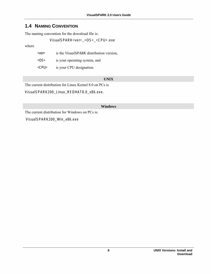
1.4 NAMING CONVENTION The naming convention for the download file is:
VisualSPARK<ver>_<OS>_<CPU>.exe where
<ver> is the VisualSPARK distribution version,
<OS> is your operating system, and
<CPU> is your CPU designation.
UNIX The current distribution for Linux Kernel 8.0 on PCs is
VisualSPARK200_Linux_REDHAT8.0_x86.exe.
Windows The current distribution for Windows on PCs is:
VisualSPARK200_Win_x86.exe
6 UNIX Versions: Install and Download

VisualSPARK 2.0 Users Guide
2 UNIX VERSIONS: DOWNLOADING AND INSTALLATION INSTRUCTIONS FOR RED HAT LINUX 8.0 (INTEL PROCESSORS)
2.1 REGISTRATION VisualSPARK installation requires a password. The password was sent to you by email after you completed the registration form.
2.2 OTHER SOFTWARE REQUIRED • GNU make
• GNU g++ compiler and libraries
• Adobe Acrobat Reader program for viewing .pdf files ( acroread ). Download from http://www.adobe.com/products/acrobat/readstep2.html .
For Linux the download URL is ftp.adobe.com/pub/adobe/acrobatreader/unix/5.x/linux-506.tar.gz. Download this file into a temporary directory. Unpack the file using the command % tar xzf linux-506.tar.gz <Enter>
then follow the installation instructions in the readme file.
• The Netscape program for viewing the html files. Linux operating systems may already have the above software; however, if they are not installed on your computer, ask your system administrator to install them.
The executables of these programs (make, g++, acroread) must be accessible by your PATH environment variable. The installation setup program checks the above requirements and gives appropriate error messages.
2.3 INSTALL VISUALSPARK • To download, right click the following link and select Save Link As from the menu:
VisualSPARK200_Linux_REDHAT8.0_x86.exe. In the “Save As...” panel: Make sure the Selection field contains your home directory followed by the file name VisualSPARK200_Linux_REDHAT8.0_x86.exe then click OK
• After the file save is complete, make the downloaded file executable by running the command (where % is the command prompt and user-entered text is in bold): % chmod +x VisualSPARK200_Linux_REDHAT8.0_x86.exe <Enter>
• Run the downloaded program (supply the installation password when it is asked for): % ./VisualSPARK200_Linux_REDHAT8.0_x86.exe <Enter>
This will extract the VisualSPARK distribution files starting at directory $HOME/vspark200.
• Run the following two commands to start the install program: % cd $HOME/vspark200/install <Enter> % ./install <Enter>
7 UNIX Versions: Install and Download

VisualSPARK 2.0 Users Guide
This will modify your .cshrc , .profile , .bash_profile files, and add the SPARK environment settings. It will also create the following files in the $HOME/vspark200 directory: classpath.env , projects.env , sparkenv.csh , sparkenv.sh
• Logout and then login to make the new environment variable changes become effective.
• To start VisualSPARK (first make sure that the X-windowing system is running) type the command: % vspark & <Enter>
2.4 UNINSTALL VISUALSPARK To uninstall VisualSPARK, run the following commands to start the uninstall program:
% cd $HOME/vspark200/install <Enter>
% ./uninstall ; cd $HOME <Enter> Uninstallation will remove the VisualSPARK installed files in the directory $HOME/vspark200. It will also remove the SPARK-related environment settings from the .cshrc, .profile, .bash_profile files.
If there are user-created files in the $HOME/vspark200 directory tree, they will not be removed, and a message will be given to the user to check them and remove the $HOME/vspark200 directory manually.
8 UNIX Versions: Install and Download

VisualSPARK 2.0 Users Guide
3 WINDOWS VERSIONS: DOWNLOADING AND INSTALLATION INSTRUCTIONS FOR WINDOWS 95/98/ME/NT/2000
3.1 REGISTRATION VisualSPARK installation requires a password. The password was sent to you by email after you completed the registration form.
3.2 OTHER SOFTWARE REQUIRED The Acrobat Reader program version 5.0 or later from Adobe is needed for viewing the VisualSPARK help files. If this program is not already installed on your computer you can download it from
http://www.adobe.com/products/acrobat/readstep2.html.
3.3 INSTALL VISUALSPARK • To download, click VisualSPARK200_Win_x86.exe.
• In the “File Download” panel, select Save this program to disk and save to a temporary directory (e.g., C:\temp). The file name is VisualSPARK200_Win_x86.exe.
After the downloaded file is saved, make sure its size is the same as the number mentioned above. To find out the size (in bytes) of the downloaded file, right click the file inside the Windows Explorer and select Properties from the menu.
• After the file save is complete, run the program VisualSPARK200_Win_x86.exe. (e.g., click Start, click Run..., type C:\temp\VisualSPARK200_Win_x86.exe, click OK.)
Alternatively, with the Windows Explorer, go to the directory where VisualSPARK200_Win_x86.exe was saved (e.g., C:\temp) and double click on VisualSPARK200_Win_x86.exe.
• Follow the instructions that appear on your screen for installing VisualSPARK.
3.4 UNINSTALL VISUALSPARK To uninstall VisualSPARK, go to the Windows Start › Settings › Control Panel › Add/Remove Programs menu. Select the VisualSPARK entry and click the Add/Remove button.
3.5 SPECIFY TARGET C++ COMPILER By default the VisualSPARK package for Windows installs the mingw C++ compiler program g++. After VisualSPARK has been successfully installed, it is possible to change the target C++ compiler that will be used by SPARK to build the libraries of atomic classes.
To switch to the Microsoft Visual C++ compiler1, go to the install directory of the VisualSPARK installation and type the command: sh config.sh compiler=vc <Enter>
1 This release supports the VC++ compiler version 6 and more recent versions.
9 Windows Versions: Install and Download

VisualSPARK 2.0 Users Guide
Make sure that the file vcvars32.bat is copied from the Microsoft Visual Studio bin directory to the bin directory of the VisualSPARK installation.
To switch back to the mingw compiler, type the command:
sh config.sh compiler=gcc <Enter>
10 Windows Versions: Install and Download

VisualSPARK 2.0 Users Guide
4 VISUALSPARK ENVIRONMENT SETTINGS In the following text, <spark_dir> refers to the full path where VisualSPARK is installed. E.g.,
UNIX $HOME/vspark200
Windows C:\vspark200
4.1 ENVIRONMENT VARIABLES
4.1.1 SPARK_DIR
This environment variable contains the path where SPARK is installed, same as <spark_dir> mentioned above.
UNIX It is set at the end of $HOME/.cshrc , or $HOME/.profile , or $HOME/.bash_profile
Windows It is set in the file <spark_dir>\sparkenv.bat
4.1.2 PATH
Your PATH environment variable must contain <spark_dir>/bin and the directory containing the GNU g++ compiler (preferably at the front of the list); e.g., PATH might look like:
UNIX
.:$SPARK_DIR/bin:/usr/local/bin:/usr/gnu/bin ....etc
It is set at end of $HOME/.cshrc, or $HOME/.profile, or $HOME/.bash_profile
Windows
<spark_dir>\bin;<spark_dir>\gccmingw\bin;<spark_dir>\unixutil
It is set in the file <spark_dir>\sparkenv.bat
4.1.3 SPARK_PDFVIEWER
Contains the path of the Adobe Acrobat Reader program Acroread that is used for viewing .pdf files.
11 Environment Settings

VisualSPARK 2.0 Users Guide
4.1.4 SPARK_HTMVIEWER
Contains the path of the browser program ( Internet Explorer or Netscape ) that is used for viewing .htm and .html files.
4.1.5 SPARK_CHMVIEWER
Windows Contains the path of the .chm file viewer program ( named hh.exe ). Required only for Windows installation.
4.2 ENVIRONMENT FILES
4.2.1 classpath.env
This file stores the path lookup list for finding SPARK classes.
UNIX <spark_dir>/classpath.env
Windows <spark_dir>\classpath.env
It contains one line of text in the form:
SPARK_CLASSPATH=.,../class,<spark_dir>/globalclass,<spark_dir>/hvactk/class
This means the SPARK class search order is:
1. the current project directory,
2. ../class directory relative to the current project directory,
3. globalclass directory of VisualSPARK distribution, 4. hvactk classes directory of VisualSPARK distribution.
UNIX and Windows use the same syntax, with the forward slash as the path separator. There must be no spaces in the paths. This file is created by the install program. You can modify it to include users own class directories. It is used by the VisualSPARK interface as default value. VisualSPARK keeps track of the SPARK_CLASSPATH on a per-project basis. It is always used by the command line interface.
4.2.2 projects.env
This file stores the path where the current VisualSPARK projects reside.
UNIX <spark_dir>/projects.env
Windows <spark_dir>\projects.env
It contains one line of text in the form:
SPARK_PROJECTS=<spark_dir>/examples
12 Environment Settings
VisualSPARK 2.0 Users Guide
This file is created by the install program, and managed by the VisualSPARK interface. Windows can use either forward or backward slash as path separator.
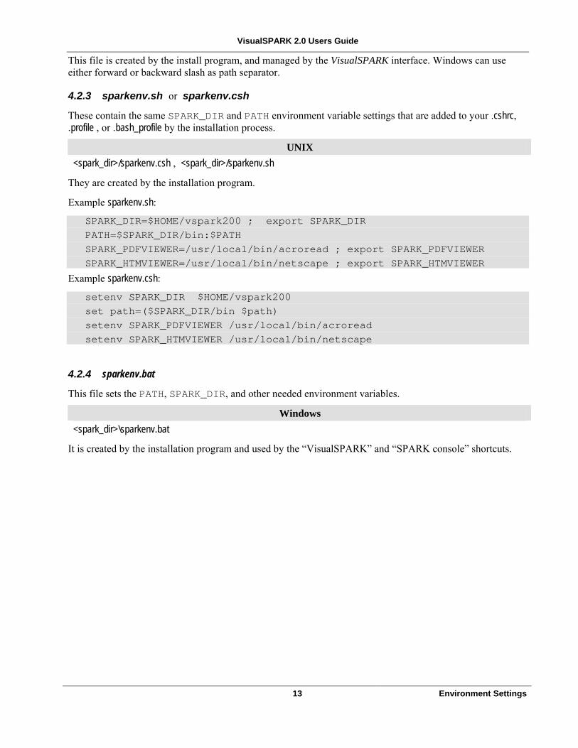
4.2.3 sparkenv.sh or sparkenv.csh
These contain the same SPARK_DIR and PATH environment variable settings that are added to your .cshrc, .profile , or .bash_profile by the installation process.
UNIX <spark_dir>/sparkenv.csh , <spark_dir>/sparkenv.sh
They are created by the installation program.
Example sparkenv.sh:
SPARK_DIR=$HOME/vspark200 ; export SPARK_DIR
PATH=$SPARK_DIR/bin:$PATH
SPARK_PDFVIEWER=/usr/local/bin/acroread ; export SPARK_PDFVIEWER
SPARK_HTMVIEWER=/usr/local/bin/netscape ; export SPARK_HTMVIEWER
Example sparkenv.csh:
setenv SPARK_DIR $HOME/vspark200
set path=($SPARK_DIR/bin $path)
setenv SPARK_PDFVIEWER /usr/local/bin/acroread
setenv SPARK_HTMVIEWER /usr/local/bin/netscape
4.2.4 sparkenv.bat
This file sets the PATH, SPARK_DIR, and other needed environment variables.
Windows <spark_dir>\sparkenv.bat
It is created by the installation program and used by the “VisualSPARK” and “SPARK console” shortcuts.
13 Environment Settings

VisualSPARK 2.0 Users Guide
5 COMMAND LINE EXECUTION OF SPARK
5.1 THE SPARK DIRECTORY STRUCTURE
Figure 1: SPARK Directory Structure
SPARK is composed of many files kept in several directories (see Figure 1). The root directory where SPARK is installed is named after the version number, i.e., vspark200/.
The bin, lib and visspark subdirectories contain the fixed executable code and binary libraries2 used by SPARK and the graphical user interface. The install subdirectory contains information related to the installation of VisualSPARK. This information is required for removal of VisualSPARK with the uninstall process and should not be disturbed. Necessary source code header files are in the inc subdirectory. The doc subdirectory in the VisualSPARK directory contains user reference documents for both SPARK and VisualSPARK.
SPARK comes with two class libraries, the global classes and the HVAC ToolKit classes. The global classes are in the globalclass subdirectory and include the basic mathematical functions likely to be needed in many SPARK problems, regardless of application area. The subdirectory integrators contains source files used to implement the advanced integration methods in globalclass.
The HVAC ToolKit classes in the hvactk subdirectory define a modest library for modeling heating, ventilation, and air-conditioning systems. The examples directory contains examples of SPARK problems using the global classes. Also, there is a compressed file in the hvactk subdirectory that contains sample problems for all classes in the HVAC library. A utility, testhvac, is provided to extract, build, and execute these sample problems.
In SPARK, each new problem must be in its own directory, called a project directory. This directory is used to store the problem file (problem.pr) and related files such as input (problem.inp), output (problem.out), log files, and various intermediate files produced in a SPARK run.
Problems that are related are often grouped under a common parent directory, called the projects directory (plural). The projects directory, which can have any name, should also have a class subdirectory to hold any new classes you may create for the various problems under projects. The above mentioned examples subdirectory is an example of a projects directory. As can be seen in Figure 1, there are seven project subdirectories under examples: 2sum, 4sum, example, frst_ord, room_fc, room_fc_commandLineOnly and spring.
When using the VisualSPARK interface the directory structure is extended by the addition of one or more input set subdirectories under each project directory. This is to allow you to have more than one set of inputs for each problem. VisualSPARK places input, output, and other files that are specific to a particular input set in the input set directory.
2 Source is not provided for modules that are provided in binary form in the bin and lib subdirectories.
14 Command-Line Execution

VisualSPARK 2.0 Users Guide
5.2 COMMANDS UNIX
You may execute SPARK under UNIX or Linux with the VisualSPARK graphical user interface (Section 6), or with commands issued in an xterm command window. In this section we focus on the xterm command window (although any X-system terminal can be used
As noted previously, each SPARK problem should be in its own project directory. The SPARK problem file created by the user resides there, as well as various related files created as SPARK runs. The current working directory should be set to the project directory before running SPARK. We assume this is so in the following examples.
Windows You may execute SPARK either with the VisualSPARK graphical user interface (Section 6), or with commands issued in an MSDOS command window. In this section we focus on the MSDOS command method.
It is important to note that the following commands, e.g., gmake and runspark, do not have an argument indicating a particular problem to be run. This is because it is assumed that there is only one file in the project directory with the .pr extension. Consequently, if you want to have different versions of your problem you must place them in different project directories.
5.3 PREPARATIONS UNIX
Running a SPARK problem from the command line requires that the bin subdirectory of the directory where VisualSPARK is installed be in your PATH. The VisualSPARK installation process modifies your profile file so as to make this change to your PATH.
Another requirement for running a SPARK problem is that the classpath.env file in the $(SPARK_DIR) directory contains a path to the SPARK class files used in the problem to be solved. As created by the VisualSPARK installation (See Section 4.2.1), the class path includes the current project directory (i.e., the current working directory), the ../class directory, and all directories containing classes that came with the VisualSPARK distribution. If you have classes elsewhere, you must to edit the classpath.env file accordingly.
One final requirement is that a makefile be defined in the project directory, i.e., $(SPARK_DIR)/examples/2sum in this example. Assuming the Linux bash or UNIX Bourne shell, you can do this with the commands:
% cd example/2sum <Enter>
% ln -s $SPARK_DIR/lib/makefile.prj makefile <Enter>
This creates makefile as a symbolic link in the current directory to the master SPARK make file, makefile.prj, which resides in the $(SPARK_DIR)/lib directory.
15 Command-Line Execution

VisualSPARK 2.0 Users Guide
Windows Running a SPARK problem from the command line requires that the $(SPARK_DIR)\bin and certain other directories be in your PATH. For the sake of clarity let’s assume that VisualSPARK is installed in the d:\vspark200 directory.
Under Windows, you can accomplish this by opening an MSDOS window and executing the sparkenv command from your $(SPARK_DIR) directory, i.e., the d:\vspark200 directory:
d:\>cd vspark200 <Enter>
d:\vspark200> sparkenv <Enter>
Alternatively, you can just select “SPARK Console” from the Windows Start › Programs › VisualSPARK menu choices. This launches an MSDOS window, changes to the d:\vspark200 root directory, and automatically runs the sparkenv.bat command file.
There are two additional tasks preliminary to running a SPARK problem at the command line. One is to be sure that the classpath.env file contains the correct path for the classes used in the problem. If you are using only the provided classes, the default values shown in Section 4.2.1 will be sufficient. Otherwise, use your text editor to modify classpath.env to include paths to your classes.
The other task is to provide a makefile in the project directory. One way to do this is to simply copy the master make file, makefile.prj, from the d:\vspark200\lib directory to the project directory, i.e., d:\vspark200\examples\2sum in this example:
d:\vspark200> cd examples\2sum <Enter>
d:\vspark200\examples\2sum> copy d:\vspark200\lib\makefile.prj makefile <Enter>
5.4 BUILD AND RUN UNIX
Once you have thus set the environment, you are ready to run SPARK to solve the problem. This can be done with the gmake command issued from the project directory. The command to run the problem is then:
% gmake run <Enter>
Since no make file is given in the command line, gmake uses the symbolic link makefile that was created previously. This make file orchestrates the various steps needed to create the executable program3 and run that program to solve the problem (see SPARK Reference Manual).
Windows Once you have carried out these tasks, you are ready to run SPARK to solve your problem. This can be done with the gmake command issued from the project directory. The command to run the problem in project is then:
d:\vspark200\examples\2sum> gmake run <Enter>
This gmake command will use either the local makefile, or the link to the master makefile.prj, to orchestrate the various steps needed to build the executable solver program, and run that program to solve the problem.
3 The executable solver program is also referred to as the simulator program.
16 Command-Line Execution
VisualSPARK 2.0 Users Guide
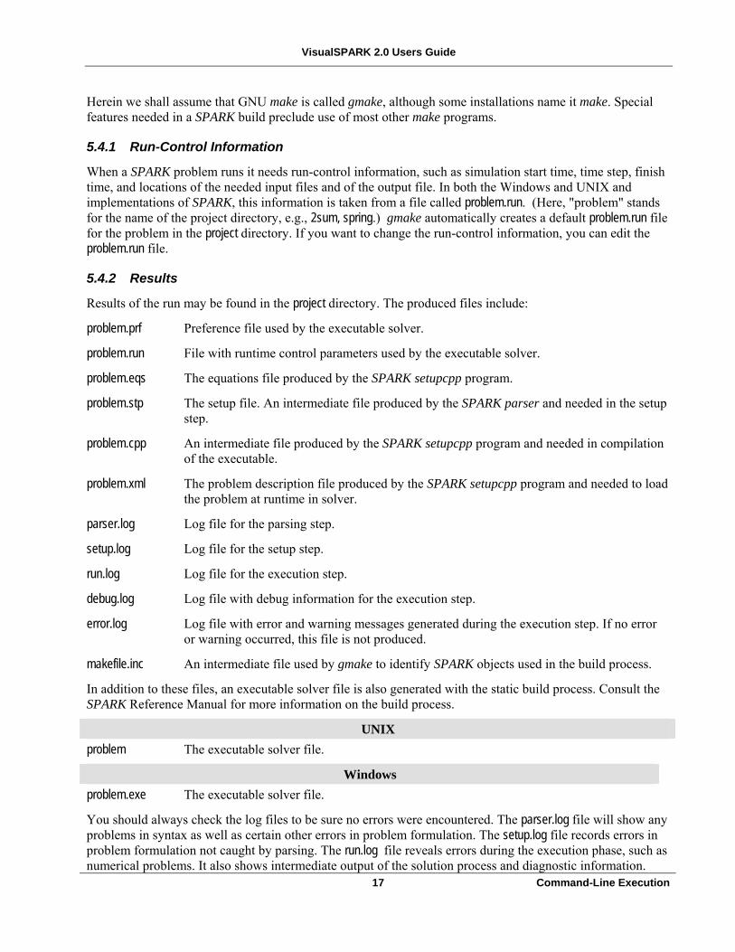
Herein we shall assume that GNU make is called gmake, although some installations name it make. Special features needed in a SPARK build preclude use of most other make programs.
5.4.1 Run-Control Information
When a SPARK problem runs it needs run-control information, such as simulation start time, time step, finish time, and locations of the needed input files and of the output file. In both the Windows and UNIX and implementations of SPARK, this information is taken from a file called problem.run. (Here, "problem" stands for the name of the project directory, e.g., 2sum, spring.) gmake automatically creates a default problem.run file for the problem in the project directory. If you want to change the run-control information, you can edit the problem.run file.
5.4.2 Results
Results of the run may be found in the project directory. The produced files include:
problem.prf Preference file used by the executable solver.
problem.run File with runtime control parameters used by the executable solver.
problem.eqs The equations file produced by the SPARK setupcpp program.
problem.stp The setup file. An intermediate file produced by the SPARK parser and needed in the setup step.
problem.cpp An intermediate file produced by the SPARK setupcpp program and needed in compilation of the executable.
problem.xml The problem description file produced by the SPARK setupcpp program and needed to load the problem at runtime in solver.
parser.log Log file for the parsing step.
setup.log Log file for the setup step.
run.log Log file for the execution step.
debug.log Log file with debug information for the execution step.
error.log Log file with error and warning messages generated during the execution step. If no error or warning occurred, this file is not produced.
makefile.inc An intermediate file used by gmake to identify SPARK objects used in the build process.
In addition to these files, an executable solver file is also generated with the static build process. Consult the SPARK Reference Manual for more information on the build process.
UNIX problem The executable solver file.
Windows problem.exe The executable solver file.
17 Command-Line Execution
You should always check the log files to be sure no errors were encountered. The parser.log file will show any problems in syntax as well as certain other errors in problem formulation. The setup.log file records errors in problem formulation not caught by parsing. The run.log file reveals errors during the execution phase, such as numerical problems. It also shows intermediate output of the solution process and diagnostic information.

VisualSPARK 2.0 Users Guide
The equations file shows the a user-readable calculation sequence followed by SPARK to solve the problem. It is explained in detail in the Reference Manual.
5.4.3 The runspark Command
UNIX To simplify the UNIX SPARK solution procedure described above, there is a script file called runspark in the directory $(SPARK_DIR)/bin. This script file is used by typing (in the current project directory):
% runspark <Enter>
It will make the symbolic link to the SPARK make file, employ the current classpath.env file, and run the problem in the current directory. To get the usage information about runspark type:
% runspark -help <Enter>
To clean current project directory type:
% runspark clean <Enter>
Windows To simplify the command line SPARK solution procedure described above, there is a command file called runspark.bat in the directory $(SPARK_DIR)\bin, i.e., d:\vspark200\bin. This command file is run by typing (in the current project directory):
d:\vspark200\examples\2sum> runspark <Enter>
It will make the symbolic link to the SPARK master make file, supply the default classpath.env file, and run the problem in the current directory. To get the usage information about runspark type:
d:\vspark200\examples\2sum> runspark –help <Enter>
To clean current project directory type:
d:\vspark200\examples\2sum> runspark clean <Enter>
This removes all files created during a previous run.
5.4.4 The runspark Flags
The following flags are not set by default unless you specify them at the command-line followed by “=yes” to activate them.
Flags Description
SPARK_DEBUG Builds a SPARK simulator that uses the DEBUG solver library.
SPARK_STATIC_BUILD Builds a self-contained SPARK simulator that does not need to load the problem description at runtime.
5.4.5 Re-running a Problem Executable
As noted above, once you have run the problem by either of the above methods, the problem description file named problem.xml will be in the project directory, along with a problem preference file, problem.prf and a runtime control file, problem.run. The problem.prf file contains the numerical solution settings for each component of the problem. 18 Command-Line Execution

VisualSPARK 2.0 Users Guide
If it is desired to run the numerical solution stage again, it can be initiated by executing the SPARK solver program sparksolver4 with problem.prf, problem.run , and problem.xml as arguments.
UNIX
% sparksolver problem.prf problem.run problem.xml <Enter>
Some UNIX installations, notably Linux, may not automatically include the current working directory “.” in your PATH. If “.” is not in your PATH, you must prefix the problem executable with “./”.
Windows
d:\vspark200\examples\2sum> sparksolver 2sum.prf 2sum.run 2sum.xml <Enter>
Alternatively, you can again enter the command gmake run <Enter>
with little loss of efficiency, since gmake will not rebuild the problem if nothing has changed. On the other hand, if you do make changes to any of the classes or the problem file, you must use gmake to rebuild.
It is important to note that the above gmake and runspark commands do not have an argument indicating a problem file to be run. This is because it is assumed that there is only one problem file in the project directory with the .pr extension. Consequently, if you want to have different versions of your problem you must place them in different project directories.
5.5 EXAMPLES As can be seen in Figure 1, there are several project subdirectories under the examples subdirectory. These contain problem specification files (.pr) and input files (.inp) from the examples in the SPARK Reference Manual. A good one to start with is 4sum.p. This problem simply adds four inputs, x1, x2, x3, and x4, with values taken from a provided input file 4sum.inp, producing their sum, x7.
UNIX To run the 4sum example using the detailed steps indicated in the previous section, go to the 4sum directory and set the class path and symbolic to the SPARK make file:
% cd $SPARK_DIR/examples/4sum <Enter>
% ln -s $SPARK_DIR/lib/makefile.prj makefile <Enter>
The next step is to build the solver for the problem and run the problem:
% gmake run <Enter>
This results in creation of an executable program called 4sum. Several other files are created, including 4sum.prf which is needed to execute 4sum, and 4sum.run which provides run-control information. The command also runs the executable. When the command completes, the results can be found in 4sum.out which can be examined with vi, Emacs, or other UNIX editors. You should also examine the various log files noted in the previous section.
We see that the inputs for x1 through x4, read from 4sum.inp, were all 1, so their sum is 4. As before, these
4 This approach of running a problem executable assumes that the problem is dynamically built at runtime from its description contained in the problem.xml file. Consult the SPARK Reference Manual for more information on the build process.
19 Command-Line Execution

VisualSPARK 2.0 Users Guide
results are also placed in 4sum.out.
Windows
To run the 4sum example using the detailed steps indicated in the previous section, go to the 4sum directory and set the class path and symbolic link to the SPARK make file:
d:\> cd d:\vspark200\examples\4sum <Enter>
d:\vspark200\examples\4sum> ln -s d:\vspark200\lib\makefile.prj makefile <Enter>
The next step is to build the solver for the problem and run the problem:
d:\vspark200\examples\4sum> gmake run <Enter>
This results in creation of an executable program called 4sum.exe. Several other files are created including 4sum.prf, which is needed to execute 4sum, and 4sum.run, which provides run-control information. The command also runs the executable. When the command completes, the results can be found in 4sum.out, which can be examined with Notepad or another Windows or MSDOS editor. You should also examine the various log files noted in the previous section.
We see that the inputs for x1 through x4, read from 4sum.inp, were all 1, so their sum is 4. As before, these results are also placed in 4sum.out.
5.6 USING SPARK OUTPUT SPARK output files, i.e., problem.out, can be viewed with any text editor or viewer available on your computer. However, if the output is voluminous, such as for a dynamic simulation over a long time period, output is better viewed graphically, perhaps using a spreadsheet or plotting program that you may have installed. One option for UNIX command line users is the gnuplot program, available free at several Internet sites.
The VisualSPARK Graphical User Interface contains a plotting program that allows you to view the SPARK output file graphically. See Section 6.6 for more details. The tutorial in this document also shows usage of the plotting package.
20 Command-Line Execution

VisualSPARK 2.0 Users Guide
6 USING THE GRAPHICAL USER INTERFACE (GUI)
6.1 THE MAIN VISUALSPARK WINDOW The VisualSPARK graphical user interface for the Microsoft Windows and UNIX environments is available as a more user-friendly environment than the command line.
UNIX To use it, the X Window System must be running. If you have not yet started X, do so with the command appropriate for your system. Under Linux, for example, this would be:
% startx <Enter>
Then you must open a terminal command window, often available from your X desktop or menus. In this window enter:
% vspark & <Enter>
This will open the VisualSPARK main window on your X desktop as shown in Figure 2 (p. 22). The screen shots in this document were obtained on a Windows platform. In the UNIX environment, the visual elements will look a bit different.
Windows You can start VisualSPARK in either of two ways:
You can go to the VisualSPARK root directory, e.g., d:\vspark200, and type:
d:\vspark200> visspark <Enter>
You can select VisualSPARK from the Windows Start › Programs › VisualSPARK menu.
Either method will open the VisualSPARK main window on your Windows desktop as shown in Figure 2.
This screen has three principal panels, labeled “Projects”, “Class Directories”, and “Classes”, as well as command menu bars across the top and down the left side. The commands available in the menu bars will change depending upon which panel is active. A panel becomes active when you click your left mouse button while the cursor is in it. When the cursor is on a menu bar button, a brief description of what it does is presented in a pop-up window.
21 Using the GUI

VisualSPARK 2.0 Users Guide
Figure 2: VisualSPARK main window
Figure 3: Projects directory tree
The “Projects” panel shows currently available projects upon which you can work. At the top of this panel there is an open folder icon, symbolizing a currently active Project Directory. Holding the cursor over the word “Projects” in front of the folder icon causes the complete, current project path to be displayed in a pop-up window. Clicking on the folder opens a directory tree showing where this project folder is placed in your file system, Figure 3.
If you wish, you can change to a different Projects directory by clicking on the desired folder in the tree.
Typically, a Projects folder will have several Project subdirectories with individual projects, i.e., SPARK problems. In turn, each project can have one or more subdirectories, e.g., 2sum_inp below 2sum. These subdirectories represent particular input sets for the project, so you can run the problem with different input data and run-control information.
In order to execute SPARK, one of these input set directories must be selected.
22 Using the GUI

VisualSPARK 2.0 Users Guide
Figure 4: Help menu
The “Classes” panel shows the classes in the directory currently selected in the “Class Directories” panel. Double clicking one of these classes, or selecting a class and pressing the Edit Class button, opens the class file for editing.
To view the structure of a project or class/object, in the main panel, right-click on either a project name or class file and choose Show class tree from the menu. This will pop up a new window showing the tree structure of the object. There are two main views: classes only and full structure with object names. These views are selected by radio buttons at the top of the panel:
Figure 5: Class tree
23 Using the GUI

VisualSPARK 2.0 Users Guide
If the Show full structure button is selected, the variable name associated with the object is shown with the class of the object in parentheses. If the Show classes only button is pressed, only one occurrence of each class is shown at each level. The lower radio buttons show more or fewer levels of the tree structure.
Figure 6: Class tree showing full structure
Figure 7: Class path for the room_fc project (but not for individual objects)
If the mouse is positioned over an entry in the tree, the class path of that object is shown in a popup window. The tree may be printed on a PostScript compatible printer with or without the class paths by checking the button below the printer icon. Multiple class tree windows may be displayed, and by right-clicking on an object lower in the tree and choosing Show class tree from the menu that object and its subtree will appear in a new window. Here are two examples of the PostScript output of a tree. Figure 7 shows the class path for the project room_fc but not for the individual objects. Figure 8 shows the class path for each object.
Figure 8: Class path for each object
Note the Rescan buttons below the “Projects” and “Classes” panels. While VisualSPARK can often automatically update the panel displays for changes made, it may not be aware of certain changes, e.g., adding a new project. The Rescan button forces panel update to deal with these situations.
24 Using the GUI

VisualSPARK 2.0 Users Guide
Figure 9: “Save class path” dialog box
The “Class Directories” panel shows class directories currently available for use in the project selected in the “Projects” panel. These are initially set to the classes defined in the classpath.env file (see Sections 2.3 and 3.3), but these paths may be rearranged or new paths added with the Modify button at the bottom of the panel. Once changed, the new class path may be saved with the project or for the current set of projects or for all of your VisualSPARK Projects (See Figure 9).
The command menu across the top of the VisualSPARK main screen offers functions related to controlling VisualSPARK, such as Quit and Help, or editing classes and projects.
25 Using the GUI

VisualSPARK 2.0 Users Guide
Button Name Function Text Editor This button applies to either Projects or Classes. It executes a text editor and loads the
selected file for editing. The label on this button changes depending on cursor location. When in the “Projects” panel the label is “Edit Project”, and it changes to “Edit Class” when you move to the “Class” panel. When the cursor is not in either of these panels, the button is inactive and labeled “Text Editor”.
Delete Selected This button will delete the selected file, whether it is a project, an input set, or a class.
Help This button offers a menu with selections for various on-line SPARK documents as seen in Figure 4 (p. 23).
Quit Exits the VisualSPARK interface.
The menu to the left of the “Projects” panel offers functions related to singular operations with SPARK projects. The buttons available at any time are determined by what is selected in the three panels. For example, if a project is selected in the “Projects” panel, only the Project and New Input Set buttons are available. Clicking on the Project button opens the Project menu (Figure 10); this allows creating or copying a project, as well as other options. The New Input Set button allows you to create input data for the selected project. On the other hand, if an Input Set is selected in the “Project” panel, the buttons for editing the input set, running the project and plotting results or changing preferences become available. These menu commands are explained in more detail in subsequent sections.
6.2 THE PROJECT MENU
6.2.1 Creating and Copying Projects
Figure 10: Project menu
Clicking on the Project button opens the Project menu as seen in Figure 10. From this menu you can create a new project either by starting fresh, or by copying an existing project. Note that any new project created will be placed under the Projects directory currently appearing in the “Projects” panel. Therefore you should be sure you are in the correct Projects directory before clicking the Project button (See Section 6.2 ).
If you select New Project, you will be asked for a new project name in a dialog, and then a text editor (Figure 12) will be opened with an empty file. After typing the SPARK problem definition into this file, saving will create a new subdirectory for it in the Projects directory and the new project will then appear in the “Projects” panel.
The Copy from selected menu entry is available if there is at least one project in the Projects directory. Clicking on it will pop up a dialog in which you can enter the name for the new project, as seen in Figure 11. As before, the new (copied) project will be placed in the current Projects folder and displayed in the “Projects” panel.
26 Using the GUI

VisualSPARK 2.0 Users Guide
Thereafter, you can open it with the Text Editor button on the main window, (which will now be labeled “Edit Project”) or simply click on it.
Figure 11: Copy project dialog
Figure 12: “Edit New Project” text editor window.
6.2.2 Make Package, Make Clean, Make CleanALL
As can be seen in Figure 10, the Project menu has three Make options. These are provided for project file maintenance tasks that may need to be done occasionally. The Make Clean option removes various intermediate and results files from a project. This needs to be done sometimes because problem errors can result in incomplete builds, leaving the project in an improper state. Make Clean will allow a fresh start on the problem after you have fixed the errors. No user-created files will be deleted. Make CleanALL is similar, but does a more thorough cleanup and deletes all run subdirectories created by VisualSPARK. The Make Package option allows export of a project. It copies all files related to the project, including its class files, into a new directory called projName_pkg, where projName is the name of the project being packaged. By sending this directory to a colleague, you can be sure he/she will have all necessary files to run the project.
6.3 NEW INPUT SET OR EDIT INPUT SET After creating a new project you would typically then want to create an input set for it. The New Input Set button in the main VisualSPARK window, Figure 2, allows you to do this. Since input sets are always associated with a particular project, a project must be selected in the “Projects” panel before this button is available. Clicking on this button brings up the “Input Editor” window shown in Figure 13.
27 Using the GUI

VisualSPARK 2.0 Users Guide
If an existing input set is selected in the “Projects” panel instead of just a project, the Edit Input Set button will be available. Clicking it will launch the same editor as used for creating new input sets. In this case, however, the fields will contain existing values.
At the top of the “Input Editor” window is a Set File menu choice, under which you will find the familiar Open, Save, Save As, and Close choices.
Figure 13: “VisualSPARK Inputs” window.
To the right are several buttons which will bring the labeled windows to the top of the stacking of VisualSPARK windows. For example, if you are working in the input editor, and you cannot see the main VisualSPARK window, press the Main Window button and it will bring it to the top of all other windows on your computer. If the window doesn’t yet exist (e.g., the graph window) the button has no effect.
Below there is a tool bar with the normal icons for Open, Save, and Close. To the right of the tool bar is a field showing the name of the current input set file.
6.3.1 Input Editor
The input editor has three panels below the tool bar. At the upper left is an area to put useful comments about the data set. Below that is a panel with three tabs labeled “Values for Input Variables”, “Initial Predictor Values (Breaks)” and “Initial Values for Dynamic Variables”. These tabbed areas show all variables in those categories.
The tab “Values for Input Variables” contains the values for the variables that act as inputs to the model. The tab “Initial Predictor Values (Breaks)” contains the predicted values for the break variables that are used as predictors in the Newton-Raphson iteration. Finally, the tab “Initial Values for Dynamic Variables” contains the initial values of the dynamic variables in the model. The dynamic variables are the variables that are connected to the x port of an atomic class defined with class type INTEGRATOR (Consult the SPARK Reference Manual for more information on the integrator classes). Note that if a dynamic variable happens to be a break variable too, it will only be listed in the tab “Initial Values for Dynamic Variables” and not in the tab “Initial Predictor Values (Breaks)”.
For each tab a variable may be classified into one of two categories.
28 Using the GUI

VisualSPARK 2.0 Users Guide
Time-Varying These are input variables for which you will want to give time-varying values in the lower left panel (which is labeled “Variables → Time”).
Constant These are input variables for which you want to give constant values in the adjacent field.
You indicate the category for each variable by clicking on the radio buttons, which activates the string area where to specify the constant value or a URL.
At the top of the tab panel is a check button labeled Hide NONAMEs . This button allows you to omit SPARK NONAME variables, i.e., those that appear only inside macro objects and that have no user-assigned names. These are often quite numerous in large projects, and checking this button will avoid needless clutter in the table of variables in the “Input Editor” window.
In addition to its role in categorizing inputs, the tab panel displays other information about the variables. Shown to the right of each variable name is its units as determined from the problem definition file in the manner discussed in the Reference Manual. Additionally, note that if the window size is reduced this information may not be fully visible.
If a variable name is not fully visible (e.g. because it is too long), placing the mouse over the name will pop up a temporary window showing the full name.
The lower left panel is a table in which you can give values for each input variable categorized as time-varying in the upper left panel. The first column in the table represents time, and the others represent the input variables identified as time-varying. The first row of the table lists the names of these variables. In subsequent rows, a time value is entered in column one, followed by numerical values for the variables at that time. As explained in the Reference Manual, SPARK interpolates between the given time points to get intermediate values. The table behaves in a spreadsheet-like manner, so you can scroll up and down or left and right as needed. The buttons at the bottom allow you to Insert a row above a selected row, Add a row after a selected row, or Delete a selected row. The number of columns is determined automatically by the number of time-varying input variables. If an input variable is selected as constant, its column in the table is made “invisible”, because the value for a constant input variable is taken from the entry in the top panel.
6.3.2 Run-Time Parameters
To access the run-time parameters panel press the Run Windows button at the top of the input panel. You must enter appropriate values for each item.
For problems to be solved only once, enter 0 for both Initial Time and Final Time, any nonzero value for the Constant Time Step and Report Cycle, and 0 for First Report.
For dynamic problems, you enter appropriate values determined from the mathematical model and numerical considerations.
The Restore Initial Values button at the bottom of the panel can be used to restore the fields to values that existed when the editor was started. The two buttons above the Run-Time Parameters fields are duplicates of buttons of the same name in the main VisualSPARK window.
Diagnostic levels
At the bottom of the panel are check buttons to tell the solver to report one or more type of diagnostic information to the run log file.
The choices are:
29 Using the GUI

VisualSPARK 2.0 Users Guide
• Silent (no diagnostic output) • Convergence • Inputs • Reports • Preferences • Statistics • Requests
The diagnostic level Convergence applies only to iterative components and shows the following information at each iteration:
• the iteration count (0 corresponds to the prediction step),
• the value of the weighted Euclidean norm of all residuals comprising this component,
• the value of the weighted Euclidean norm of the increments for all unknown variables in the component, and
• for the worst-offender variable, the convergence error, tolerance, value and name. The convergence error corresponds to the increment between successive iterations for the variable in question. Consult the SPARK Reference Manual for more details on the convergence diagnostic output.
The diagnostic level Inputs shows in which input files values for the listed variables will be read from. This diagnostic is generated before the first step of the simulation.
At the end of each time step, the diagnostic level Reports shows the values of the problem variables for which the REPORT keyword was specified in the problem description.
The diagnostic level Preferences shows the list of all global and component preference settings before the first step of simulation. This allows you to verify the settings that will be used for the solution process.
The diagnostic level Statistics shows simulation statistics at the end of the simulation. This can be helpful to compare numerical performance with different set of settings for example.
Finally, the diagnostic level Requests shows when and where from a simulation request was made over the course of the simulation. This allows to track the requests generated from the atomic classes.
After making any changes to the run-time parameters you must save the values by pressing the Save button, which looks like a floppy disk. At the top of the panel is a Run button which you may use to run the model, a pull-down menu to choose graph to show results, and a Close button to close and dismiss the panel.
6.4 RUNNING
6.4.1 The Run Command
When you have properly defined a project and an input set, select the input set in the “Projects” panel and click on the Run button either in the main VisualSPARK window, Figure 2, or in the “Input Editor” window, Figure 13. This builds the solver and executes the problem solution file, much as described in Section 0. The run status box, shown in Figure 14, is displayed.
30 Using the GUI

VisualSPARK 2.0 Users Guide
Figure 14: “Run status” windows.
The check marks are displayed as the build process progresses. Provided no errors are encountered during the build, the last stage, Running Solver, will be reached. This is the numerical solution phase. When it completes, the status report box closes. Note that while the run is in progress the Run button in the main window is highlighted in bright red. No other action can be taken with the project until the first three steps are complete and the solver is started, as indicated by the status report box text. However, the Stop button may be pressed at any time to abort the process.
6.4.2 Log Files and Error Reports
Errors can arise in any of the several steps that take place as a result of the Run command. These errors are reported in various log files as discussed in Section 5.4.2. When using the VisualSPARK interface. All of the log files will automatically be opened if an error occurs. You should examine these files carefully, beginning with run.log to determine where the error occurred. For example, if we deliberately introduce spurious text in the 2sum.pr file and run it we get the parser.log file as shown in Figure 15. For run-time errors, the error.log file will be opened in addition to any others.
Figure 15: Project parser log
6.5 COMPONENT PREFERENCES The Preferences button at the bottom left of the main window, Figure 2, brings up the “Component Preference Editor” window (Figure 16) that allows you to specify advanced solution controls such as choice of solution methods5 and solution accuracy. In many instances, the default solution method and accuracy controls will suffice, so you usually do not have to change anything. However, if the solution fails, you may want to visit this dialog.
6.5.1 “Defaults/Global/Structure” Tab
The first tab labeled “Defaults/Global/Structure” in the “Component Preference Editor” window contains three sections. The left half shows the problem structure in a tree view. The inverses are first followed by input and unknown variables. By clicking on the plus “+” symbol you may expand each level of the tree. The top part of the right half contains a set of default values which will be used for the different components unless they are overridden by the user in those tabs. The bottom part contains two global values, Tolerance and MaxTolerance.
5 Some of the solution methods shown here may not be available.
31 Using the GUI

VisualSPARK 2.0 Users Guide
The Tolerance value in Figure 16 may be thought of as the maximum acceptable relative error tolerance. Iterative solution stops when the absolute difference between two successive values of each iteration variable falls below the tolerance value. Epsilon is the perturbation on the iteration variables used to calculate numerical partial derivatives. The SPARK Reference Manual should be consulted for more details on the choices available in the component preferences.
6.5.2 The Components Tabs
It is important to note that SPARK automatically decomposes your problem into separately solvable pieces called “components”. The term “component” is used here to mean a strongly connected component of the problem graph, not models of physical components. Each component can have its own solution method and accuracy specifications. Thus the “Component Preference Editor” dialog is tabbed across the top. By clicking on a particular tab you get a form for setting the controls for that component.
Since the problem considered here has a single component, Figure 16 has a single component tab for the one component plus the “Defaults/Global/Structure” tab.
The left side of the components tab shows the structure of the component, with any unknowns (i.e., break or normal unknowns) solved by the objects assigned to each of them. It is a tree structure and the levels may be viewed by clicking on the plus “+” symbols to open or close a level.
SPARK can capture diagnostic output on a component-by-component basis. There are four fields in the lower right corner of the “Component Preference Editor” window for requesting this tracing mechanism.
Figure 16: “Component Preference Editor” window.
For each tracing mechanism, the diagnostics will be written to the file designated in the file name field. The SPARK Reference Manual has more details on each tracing mechanism.
Finally, the button bar at the bottom of the “Component Preference Editor” window presents buttons to allow you to accept or reject changes made in the editor, or to seek Help. The OK button accepts all changes and leaves the “Component Preference Editor” window, while Apply accepts all changes but stays in the editor so you can make changes for other components. Cancel discards any changes you may have made to any of the components and leaves the editor.
32 Using the GUI

VisualSPARK 2.0 Users Guide
6.6 VIEWING AND PLOTTING RESULTS There are two methods that may be used to view the calculation results The first method is used to plot results from one problem in a variety of ways; the second is to plot results from several problems to make comparisons. For the first method, click Results/Plot in the main window, Figure 2, or in the “Input Editor” window, Figure 13. This brings up the menu shown in Figure 17. All choices present a popup dialog to allow you to choose the file to plot. This may either be the normal output file or the output from the trace file.
Figure 17: Results/Plot menu.
6.6.1 View results file (as text)
The top-most choice will display the results as a text file in an edit window. Results for simple algebraic problems are best viewed in this manner. The SPARK Reference Manual provides an explanation of the contents and format of this data.
6.6.2 Dynamic, 1 Variable per Plot
The next three menu choices offer different ways of plotting the results for dynamic problems. The Dynamic, 1 variable per plot choice presents the results as a sequence of plots, each with a single reported variable plotted versus time. When this button is clicked the window shown in Figure 18 appears. All problem variables with a REPORT designation in the problem file (see SPARK Reference Manual) appear in the upper panel with adjacent square selection symbols. You can select variables to be plotted by clicking on the squares, causing them to become highlighted. Automatic scaling is done for the X and/or Y axes6 if so indicated by a checked box under Auto. If an axis is not checked, you must give minimum and maximum values for scaling the axis.
When Make Graphs is clicked, a plot for each selected variable will be generated as shown in Figure 15. The Close All button will close all generated plots. Otherwise, you can close them one at a time with the Close button on each plot. Clicking on the printer icon at the bottom of the plot pops up a dialog to print the plot.
Below the scaling area there are radio buttons to add grid lines to either or both X and Y directions on the graph.
6 Note that the X and Y axes in the dialog refer to the plot horizontal and vertical axes respectively, not to the problem variable names.
33 Using the GUI

VisualSPARK 2.0 Users Guide
Figure 18: Single variable plot
dialog
Figure 19: Dynamic plot of single variable
6.6.3 Dynamic, multiple variables per plot
The Dynamic, multiple variables per plot option in Figure 17 produces a somewhat different dialog (See Figure 20). As before, variables to be plotted are selected by clicking on the adjacent squares in the top panel. However, you can designate each variable to be plotted on either a left (Y1) or right (Y2) axis. Automatic scaling is done for X and/or Y axes if so indicated by a checked box under Auto. If an axis is not checked, you must give minimum and maximum values for scaling the axis.
The “Symbols” section near the bottom contains radio buttons to specify whether the graph should show lines only without symbols, with symbols only or with lines with symbols. The entry below the buttons will limit the number of symbols shown on each curve, which will be spaced evenly along the curve. If the entry is 0, a symbol will be displayed at every data point. If it is blank, at most 20 symbols will be displayed.
In the “Scaling” area there is a pull-down menu labeled Upper X axis. After the graph is created, you may add a second time scale to the top of the graph. For example, if your graph time units are seconds you may add a scale at the top in minutes or hours, etc.
In the “Grid lines” area, you may choose grid lines for either X axis (top X1 and bottom X2) and/or Y axis (left Y1 and right Y2).
When Make is clicked, a graph with all selected variables will be displayed to the right of the dialog, as shown in Figure 21 for the room_fc problem. 34 Using the GUI

VisualSPARK 2.0 Users Guide
Clicking on the printer icon at the bottom of the plot will display a dialog for printing the graph to an installed printer.
Figure 20: Multiple plots per graph dialog
Figure 21: Multi-variable plot
6.6.4 Real-Time Dynamic Plot
Note that there is a Make Real-Time button in addition to the Make button. If the simulation runs for a long time, the Make Real-Time option allows you to see the graph developing on the screen as the solution proceeds. There are two options for the real-time plot display. When Strip Chart Window is selected, a fixed-scale, moving time axis is used, so the results appear as they would on a strip chart recorder. Otherwise, the time axis is rescaled dynamically as time advances. To use the Make Real-Time feature meaningfully you have to execute the Results / Plots › Dynamic, multiple variables per plot › Make Real-Time menu sequence while the run is in progress, i.e., before the “Run Status” window, Figure 14, has closed. Otherwise, the Make Real-Time button will produce the same plot as with Make. The Hold button just below Make Real-Time allows you to temporarily freeze the graph to examine it more closely. The label
35 Using the GUI

VisualSPARK 2.0 Users Guide
then changes to Resume, and pressing it again will allow the graph to resume updating as the solver produces more output.
6.6.5 Phase Plot
The last of the choices for plots of a single problem, Phase Plot, on the Results/Plot menu, Figure 17, is for plotting selected variables against each other, rather than against time. This option provides dialog allowing you to select the plot variables, and when Make Graph is selected the phase plot is displayed to the right of the dialog. Figure 22 shows a plot of Q_flow vs. Q_floor for the room_fc example.
Figure 22: Phase plot
6.6.6 Zooming In and Out
For all of the graph types, clicking the left mouse button in the graph area and dragging out a rectangle will zoom that area to fill the space. You may zoom in multiple times. Clicking the right mouse button will zoom out one level at a time.
Note that the plot windows shown above have been reduced in size to fit in this Guide. On the screen, they are scaled more generously, making them more readable. As with most windows on your desktop, they can be scaled dynamically to make them larger or smaller.
6.6.7 Plotting Results from Several Different Problems
For this type of plot, click Comparative Plots in the main window. A dialog will pop up in which you may choose projects and their output files for plotting.
36 Using the GUI

VisualSPARK 2.0 Users Guide
Figure 23: Select files for plotting
Figure 23 shows one output file that has been selected from several runs of a spring problem. After selecting all the desired output files, press OK and the following panel will appear.
37 Using the GUI

VisualSPARK 2.0 Users Guide
Figure 24: Multi Projects, Sets Up on One Graph
This is similar to the other plot panels except that you have the additional selection area at the top to enable/disable files from the different projects in the plot. After choosing the variables as in the other plot types, press Make Graph and the graph will appear (See Figure 25).
38 Using the GUI

VisualSPARK 2.0 Users Guide
Figure 25 Multi-Project Comparison Plot
In the legend you will see the curves grouped by variable for each problem output file. If you are not viewing this document in color, then the curves rendered in black and white can make it difficult to differentiate the curves. In addition to the different line types (dashed, solid, etc.) and different colors, different symbols can be used to distinguish the curves.
39 Using the GUI

VisualSPARK 2.0 Users Guide
6.7 EDITING PROJECTS AND CLASSES Projects (i.e., problem files) and classes can be edited within the VisualSPARK interface. There are two ways of opening existing projects or classes. The easiest way is to double click on the desired project or class in the appropriate panel in the main VisualSPARK window, Figure 2. Alternatively, you can select it in the panel and then click on the Edit button in the upper menu bar in the main window. Either method will open the associated source file in an edit window, Figure 26.
Once opened with the editor, you can make changes as needed. The SPARK Reference Manual should be consulted for information on SPARK syntax.
Figure 26: Editing projects or classes
The editor offers the basic functionality most users will be familiar with, so its operation will not be discussed at length. As can be seen, there are icons for opening, saving, printing, and closing of the file. These functions are also available under the File menu. The Edit menu offers Undo, Search, and Replace options. The Font menu allows selection of a range of font sizes. You can maneuver the insertion point with the mouse, using side and bottom scroll bars if needed. Also, there are two Go to buttons for going to specific lines in the file. The Go to line button will go to the line whose number is entered in the adjacent field. The Go to selection button also goes to a line number, but in this case the target line number is identified through selection. Typically, the selected number will be in a different window. For example, an error.log file such as shown in Figure 15 has line numbers indicating the offending line in the source file. If you select one of these line numbers in error.log by double clicking, then open the source file for editing and click on Go to selection, you will be taken to the line that needs attention.
Note that you must save the file before you run the problem or your changes will not take effect.
Always save any SPARK file after changing it!
40 Using the GUI

VisualSPARK 2.0 Users Guide
6.8 CREATING SPARK CLASSES At the bottom of the “Classes” panel in the main window, Figure 2, there is a button labeled New Class. Pressing this button brings up several options offering assistance in creation of new SPARK classes, Figure 27.
Figure 27: New Class menu
The first choice Sparksym offers symbolic algebra tools for automatic creation of atomic classes, macro classes, and SPARK problem files. This selection first brings up a dialog for entry of a name for the new class, Figure 28. After entering a name and pressing OK, a “Create Class Using Sparksym” window is opened, Figure 29.
In the field labeled "Enter the equation here" you may enter an algebraic equation to be solved by one of several symbolic algebra tools, such as Mathomatic,7 Maple, Mathematica or MACSYMA.
Figure 28: sparksym dialog
Figure 29: sparksym window
Then when Solve is pressed a complete SPARK atomic class is generated and displayed in the lower panel. When you press Save Class, the class is saved under the specified class name with a .cc extension in the active class directory. Pressing Close without first saving will result in a confirmation dialog.
In generating the atomic class, sparksym calls the chosen symbolic algebra solver to attempt to generate explicit inverse functions for every variable in the expression. If explicit inverses are not found for some variables, “implicit inverses” are used, as explained in the SPARK Reference Manual. These inverses are embedded as functions in the generated class, using names generated from the variable names. Also, every variable is placed in the class interface using a PORT statement with nominal values for INIT, MIN and MAX, and a unit string of [-], i.e., unspecified units.
7 sparksym includes a licensed derivative of the Mathomatic symbolic algebra tool. The full DOS shareware version of Mathomatic is available from www.lightlink.com/george2.
41 Using the GUI

VisualSPARK 2.0 Users Guide
Although the class is directly usable in many cases, you may want to open it with the class editor and customize it for your purposes. Additionally, you should always examine the functions carefully before use since symbolic algebra sometimes gives unexpected results.
The symbolic algebra solver that comes bundled with VisualSPARK is Mathomatic. Although not as complete as larger computer algebra systems, Mathomatic may meet many of your needs for SPARK class development. Its primary limitation is that only standard binary operations such as + (addition), – (subtraction), * (multiplication), / (division), and ^ (exponentiation), and unary minus – (e.g., the minus sign in –5), are recognized. If you find that Mathomatic does not meet your needs, you may want to install MACSYMA, Maple, or Mathematica, which are more capable symbolic algebra tools. Once you have any of these installed, you may choose them from the pull-down menu labeled Use Solver. Like Mathomatic, these options allow you to automatically create SPARK atomic classes. However, because the MACSYMA, Maple and Mathematica programs are more robust, they can generate many inverses for which Mathomatic fails. Additionally, macro classes and entire SPARK problems can be generated from given equations. The complexities of these tools prevent explanation here.
The last three options on the New Class menu, Figure 27, are for creation of new classes without use of symbolic tools. The Copy from Selected option prompts for a new class name and then creates a copy of the class currently selected in the “Class” panel, placing it in the active class directory. You should then edit the new class as needed, as discussed in Section 6.7. The two choices Create atomic class and Create macro class prompt for a new class name and then open an edit window with skeleton classes of the indicated type. These can be edited to finish creating a new class with the desired properties.
42 Using the GUI

VisualSPARK 2.0 Users Guide
7 TUTORIAL
7.1 ROOM_FC EXAMPLE
7.1.1 Getting Started
Let’s try running the room_fc (air-conditioned room) example from the examples subdirectory in the doc directory that comes with VisualSPARK. This is fully described in Section 2.4 of the SPARK Reference Manual. From (Figure 30) we see that it is one of the seven example projects. After clicking on the “+” sign to the left of the name, it opens to show that there is a data set or set-file called room_fc_inp. This contains input data along with the run-time information needed to run the model.
Notice that when you click on the “+” sign to open the project, the directories that this project uses appear in the “Class Directories” panel immediately to the right. If you click on one of those directory names, the class files in that directory will appear in the ”Classes” panel (Figure 31). Note that not all class files are necessarily used by the project, but they are available for its use.
Figure 30: Main window showing the room_fc project directory and the input
data set, room_fc_inp
Figure 31: Main window showing the classes for room_fc
Now let’s look at the SPARK code for the model itself. Reselect the project by clicking on the room_fc label and notice that the second button at the top of the VisualSPARK panel changes from Text Editor to Edit Project, signifying that if it is pressed, the editor will start with the project’s .pr (problem) file. Now press it to see the “Edit Project” screen (Figure 32).
43 Tutorial

VisualSPARK 2.0 Users Guide
Figure 32: The projects.pr (problem) file
Here, we could make changes to the problem, which is written in the SPARK language. For now, close the “Edit Project” window.
7.1.2 Running the Model
Let’s go ahead and use the room_fc model as is. Click on the input data set called room_fc_inp under the project label room_fc in the “Projects” panel of the main window (Figure 30). This selects the data set we would like to use to run the model.
Next, press Run on the main window and a “Run Status” window will pop up showing the progress of building, compiling and running the model (Figure 33). Finally, you will see a message that it is running the solver (Figure 34).
Figure 33: Building the Model
Figure 34: Running the Model
There are four steps shown in the “Run Status” window:
1. Assembling the relevant files into a C++ program (“Making project files”) 2. Compiling the C++ program and linking with the solver library (“Generating C++ program and
executable”)
44 Tutorial

VisualSPARK 2.0 Users Guide
3. Reading the data set and creating the input file for the solver (“Reading Data Set File/Writing Input File”)
4. Running the solver (“Running Solver…”) A yellow color indicates the current step. A checkmark will appear when the step is complete. You may stop the process at any time by pressing Stop.
7.1.3 Viewing the Results
Output As Text
After a run (whether successful or not), you may examine the results either as a table of numbers or as a graph. The former is achieved by choosing View results file (as text) from the Results/Plots menu in the main window. This causes the “Examine Output File” window to appear (Figure 35).
Output as Graphs
The text view is not very exciting and it is difficult to see any trends in the data. Let’s look at a graph of the data instead.
There are two major types of graphs: the dynamic plot and the phase plot. The first is a graph of the output variables versus time. The second is a plot of one variable vs. another that shows the correlation between the variables as a function of time.
Figure 35: Output in text form for the room_fc example
45 Tutorial

VisualSPARK 2.0 Users Guide
The Basic Dynamic Plot
In Dynamic Plots, you can either have a different graph for each variable to be plotted (called 1 variable per plot in the menu) or you can plot two or more variables on the same graph (called Dynamic, multiple variables per plot in the menu). Let's make a graph of multiple variables. After choosing the Dynamic multiple variables per plot from the Results/Plots menu, we select the output file, called room_fc_inp.out, from the “Choose Output File” dialog that appears Figure 36.
Figure 36: Select output file
46 Tutorial

VisualSPARK 2.0 Users Guide
Figure 37: Select variables to be plotted
After clicking on the output file name and clicking Open you are presented with a panel allowing you to choose which variables to plot, and on which of the two possible Y axes you want each variable plotted. Simply click on a green box beside each variable you want to plot (See Figure 37).
47 Tutorial

VisualSPARK 2.0 Users Guide
For now, we will leave the other settings at their default values. These settings allow you to manually scale the axes, show a “strip chart” of the data in real time as the solver runs, and control the appearance of symbols on the output curves.
Now that you’ve chosen the variables, press the Make Graph button (in Figure 37) to create the graph, (Figure 39).
Figure 38: Zooming in (dotted lines) on a portion of the graph
Now zoom in on the center of the graph where the curves make a “step” (Figure 38). Click the mouse on one corner of a rectangle that defines the area of interest, drag the mouse to the other corner, and click again. You will see a “Zoom #1” message and the rectangle. After the second button press you will see only the area you selected (Figure 40).
Figure 39: Results graph of the room_fc problem
Figure 40: Display of the zoomed portion of the results graph
You may zoom in repeatedly to see finer detail. To zoom out, press the right mouse button once for each zoom level. There is a printer icon at the bottom of the graph. Under Windows, clicking this icon will pop up the printer chooser dialog. Under UNIX (Linux, Solaris, etc.) clicking this icon will cause a print to the default printer defined in the PRINTER environment variable, or to the printer named in the entry next to the printer icon, if it is not blank.
48 Tutorial

VisualSPARK 2.0 Users Guide
Real-Time Graph
The real-time graphing feature allows you to stop the simulation if you want to check its progress or if you think it is running incorrectly. In the results plotting panel, (Figure 39), press Make Real-Time, then Run; the curves will then change as the data is written to the output file. At any time during the run you may press Hold to freeze the screen, see Figure 41. At this point the label changes to Resume, signifying that you may press it to resume screen updates. Note that after pressing the Make Real-Time button, its label changes to Stop Real-Time; you may stop the graph by pressing the button.
Figure 41: Real-time graph in progress
Strip Chart Graph
Just above the symbol control section is the scaling section (Figure 42). In it you may allow automatic scaling of the axes (the default) or choose your own minimum and maxi-mum values for the X, Y1 and Y2 axes. Note the Strip Chart Window button. During the creation of a real-time graph you may only want the latest period of data. After pressing this radio button, enter the window size in the entry to the right. This is the amount of time (along the X axis) to show in the window. This example shows the latest 20,000 seconds of data.
Figure 42: Strip chart in action
Phase Plot
The last graph type is the phase plot. With it you can see the relationship between any two variables as a function of time. Let’s take a look at the relation between Q_floor and T_floor. Choose the Phase Plot option from the Results/Plots menu and choose the output file as before. You will see the panel in Figure 43.
49 Tutorial

VisualSPARK 2.0 Users Guide
Q_floor is already selected for the X axis, so press the radio button under the “Y” for T_floor to select T_floor for the Y axis (selecting T_floor in this way will un-select Q_floor). Now press Make Graph at the bottom of the panel to create the graph in Figure 44. Here we see that the selected variables are more or less linearly related until T_floor reaches 24°C, at which point Q_floor continues to increase while T_floor stays constant. The green-filled circle indicates the first time point and the blue-filled circle the last time point.
Figure 43: Choosing the T_floor and Q_floor variables for phase
plotting
Figure 44: Phase portrait plot
50 Tutorial

VisualSPARK 2.0 Users Guide
7.1.4 Modifying the Values for the Input Variables
Let’s play a little with the input data to see how it affects the results. Click Edit Input Set in the main window. If it is grayed out (inactive) then you must reselect the room_fc_inp data set in the Projects area.
Figure 45 shows the input data editor. In the upper section is a Set File menu to load and save a data set file, and icons below that which do the equivalent. Below that is a box in which arbitrary comments may be inserted, these are saved with the data set file.
Further down there are three tabs, each listing a category of variables that may require input values to be specified. The tabs are labeled “Value for Input Variables”, “Initial Predictor Values (Breaks)” and “Initial Values for Dynamic Variables”. In the first tab that lists all the input variables for the problem, there are check buttons under the subsection labeled “Constant Value or URL” which, if pressed, allow a constant value or a Read URL from which to get data, for example a weather file. If the button is not pressed (the default) then the variable is assumed to have time-varying values, which can be entered in the table below.
The bottom section contains a table of the values for all the input variables that are checked as “time-varying.” The width of the columns may be manually changed to show longer variable names or larger values, as is the case here with the values for the variable Mcp. To change the width of a column, click the right mouse button on the vertical line between the variable-name cells and drag the mouse right or left. You should see a “+” cursor as you hold down the right mouse button.
51 Tutorial

VisualSPARK 2.0 Users Guide
Here’s where we’ll make some changes to see how they affect the results. Simply click on a cell and replace the value. Let’s make Mcp a constant variable and let's change its value to 80000, and change the T_set_low variable at time 0.0 from 23.0 to 20.0.
The “Input data editor” window should now look like the one shown in Figure 46. Note that since Mcp has been changed to a constant variable it has been removed from the “Time-varying Input Variables” table at the bottom of the window.
To change a value of a time-varying variable (T_set_low in this case), simply click on the value in the cell and enter a new value followed by the <Enter> key. Notice in Figure 46 that the 20.0 for T_set_low is red (it looks gray in printed documents), indicating that it has been changed.
Figure 45: “VisualSPARK Inputs” window.
Figure 46: “VisualSPARK Inputs” window with new values for Mcp and T_set_low
52 Tutorial

VisualSPARK 2.0 Users Guide
Also notice that the floppy disk icon at the top has changed to red (also looks gray in printed documents) indicating that something has changed in the data, and that the Run button has been disabled, i.e., clicking on Run won’t do anything. This ensures that you save any changes before making a run.
The results of a run with the new input values are shown in Figure 47. Compare this plot with Figure 39 to see the effect of changing the input values.
Figure 47: Results graph of the room_fc problem for modified input data
53 Tutorial

VisualSPARK 2.0 Users Guide
7.2 SUM5 EXAMPLE
7.2.1 Create a New Project
In this section we will create a new project and its supporting classes. The project finds the sum of five numbers. Figure 48 is a graphical representation of the problem.
After starting VisualSPARK, click the Project button and select New Project. When a dialog pops up asking for a project name, type
sum5 <Enter>
This will create a new entry in the Projects list and pop up an “Edit Project” window into which the SPARK code for the project may be typed. To minimize errors, copy and paste the following shaded text into the “Edit Project” window, Figure 49.
b
ax1
x2
x3x4x5
c
sum3
a
bsum5
sum3
sum
obj3
obj1
obj2
sum
c
sum5
x1x2x3
Figure 48: Graphical representation of a problem to find the sum of five
numbers
// Test of sum5.cm DECLARE sum5 obj ; LINK X1 obj.x1 REPORT INPUT; LINK X2 obj.x2 REPORT INPUT; LINK X3 obj.x3 REPORT INPUT; LINK X4 obj.x4 REPORT INPUT; LINK X5 obj.x5 REPORT INPUT; LINK SUM obj.sum5 REPORT ;
54 Tutorial

VisualSPARK 2.0 Users Guide
To do this on Microsoft Windows platforms, select the text with the mouse, press Control-C (which does a copy), click on the VisualSPARK edit panel and press Control-V (which does a paste). On UNIX platforms, select the text with the mouse, click on the VisualSPARK edit panel and press Control-Y (yank). You may first need to choose the text selection mode in your PDF viewer. You should now have the screen shown in Figure 49.
Figure 49: The sum5.pr “Edit Project” window
Figure 50: Select sum5 project
Now, in the “Edit Project” window click the floppy disk icon to do a Save, then click Close. In the main window click the sum5 name in the “Projects” panel (Figure 50).
55 Tutorial

VisualSPARK 2.0 Users Guide
7.2.2 Create the Supporting Classes
The Atomic Class
Now, back in the main window, in the panel labeled “Class Directories”, click on the first entry (Figure 51), the period with the project name in parenthesis, i.e. “. (sum5)” to view the class files in the project directory.
Next, under the right-most panel in the main window click on the menu button labeled New Class and choose the Sparksym entry (Figure 52). This will let us define our sum5 class using a simple equation solver called Mathomatic.
A dialog will pop up (Figure 53) asking for the name of the class. Type sum3 for the class name and click on OK. A window (Figure 53) with the title “Create class sum3 Using Sparksym” will appear. In the box labeled “Enter the equation here” type the equation sum3 = x1 + x2 + x3 and click on Solve.
Figure 51: Select class directory
Figure 52: Select sparksym entry
Figure 53: Dialog box asking for the class name (sum3)
The equation will be solved in terms of each of the variables sum3, x1, x2 and x3, and produce the SPARK programming code for the atomic class. Figure 54 shows what things should look like at this point.
Now click on Save Class to save the new class and close the window. Note that the name of the class file just created, sum3.cc, now appears in the “Classes” panel of the main window.
Figure 54: Atomic class as created with sparksym
56 Tutorial

VisualSPARK 2.0 Users Guide
The Macro Class
Going again to the main VisualSPARK window, click New Class again, but this time choose Create macro class (Figure 55).
This pops up a window labeled “Create New Class”. Enter sum5 as the name of the new class, and then click OK. A window will appear that contains, as comments, a template macro class (Figure 56).
Figure 55: New Class menu
Figure 56: “Create New Class” window showing (as comments) a template
macro class
Now edit this template by adding the following lines.
1. After the line // e.g. PORT Tin "inlet temp" [deg_C] ; add the lines PORT x1 ; PORT x2 ; PORT x3 ; PORT x4 ; PORT x5 ; PORT sum5 ;
2. After the line add the lines
// e.g. DECLARE sum Sum1, Sum2 ;
DECLARE sum obj1, obj2 ; DECLARE sum3 obj3 ; 3. After the line
add the lines // e.g. LINK Tinlet .Tin , Sum1.x , Sum2.y REPORT;
LINK .x1 , obj1.a ; LINK .x2 , obj1.b ; LINK .x3 , obj3.x1 ; LINK .x4 , obj3.x2 ; LINK .x5 , obj3.x3 ; LINK obj1.c , obj2.a ;
57 Tutorial

VisualSPARK 2.0 Users Guide
LINK obj3.sum3 , obj2.b ; LINK .sum5 , obj2.c ;
You should now have the window shown in Figure 57 (you will have to scroll down to see the link statements).
Figure 57: sum5 macro class window with added code and comments
Now click Save (the floppy disk icon) and Close.
58 Tutorial

VisualSPARK 2.0 Users Guide
7.2.3 Create the Input Data
Next, we will create some input data for the model so that we can test it out. Revisit the project sum5 by clicking on its name in the “Projects” panel and click on New Input Set to the left of the “Projects” panel. A dialog will pop up asking you for the name of the data set. Type in test under the label “Input Set Name” and click OK. The window shown in Figure 58 appears.
In the area labeled “Comments” you may put any comments that help you remember what the data set is for. Below that you will see a list of all input variables for the sum5 problem.
Figure 58: “VisualSPARK Inputs” window
You may choose to make them time-varying or constant by clicking on the radio button for each variable.
When the radio button is clicked, the area to the right of the button turns white; this indicates that you may enter the constant value or the URL string there. In the bottom section is a table where the time-varying data for the time-varying variables is entered.
The relative size of the top and bottom sections may be changed by grabbing the small square two-thirds of the way down on the right side with the mouse and dragging it up or down. Here we have moved it up a little to make more room for the data table in the bottom section.
For this problem we could either make all the inputs constant to show the solution for one set of fixed inputs or we may make them time-varying in order to have several different sets of inputs. They needn’t actually be time-varying, but we can use that concept to have multiple sets of inputs. Now enter some values for each input variable. First, click under the “Time” label in the table and enter a value of 0.0. Then, either press the right arrow key or click in the cell for variable X1 and enter 1.0. For X2 enter 2.0 and so on to X5. Be sure to press <Enter> after the last data value.
59 Tutorial
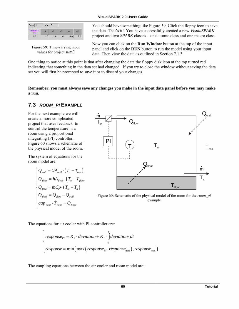
VisualSPARK 2.0 Users Guide
Figure 59: Time-varying input values for project sum5
You should have something like Figure 59. Click the floppy icon to save the data. That’s it! You have successfully created a new VisualSPARK project and two SPARK classes – one atomic class and one macro class.
Now you can click on the Run Window button at the top of the input panel and click on the RUN button to run the model using your input data. Then view the data as outlined in Section 7.1.3.
One thing to notice at this point is that after changing the data the floppy disk icon at the top turned red indicating that something in the data set had changed. If you try to close the window without saving the data set you will first be prompted to save it or to discard your changes.
Remember, you must always save any changes you make in the input data panel before you may make a run.
7.3 ROOM_PI EXAMPLE For the next example we will create a more complicated project that uses feedback to control the temperature in a room using a proportional integrating (PI) controller. Figure 60 shows a schematic of the physical model of the room.
The system of equations for the room model are:
( )(
( )
wall wall a osa
floor floor a floor
flow in a
floor flow wall
floor floor floor
Q UA T T
Q hA T T
Q mCp T TQ Q Q
cap T Q
= ⋅ −
= ⋅ −
= ⋅ − = − ⋅ =
QflowTin
Ta
m
m
Qfloor
Qwall
TosaTa
Tfloor
TPI
Figure 60: Schematic of the physical model of the room for the room_pi
example
The equations for air cooler with PI controller are:
( )( )0
min maxmin max , ,
t
PI P It
PI
response K deviation K deviation dt
response response response response
= ⋅ + ⋅ ⋅
=
∫
The coupling equations between the air cooler and room model are:
60 Tutorial

VisualSPARK 2.0 Users Guide
a sedeviation T TmCp response
= − =
t
where:
UAwall is the wall conductance [W/°C]
Tosa is the outside air temperature [°C]
hAfloor is the floor surface convection coefficient [W/°C]
Tfloor is the floor slab temperature [°C]
floorT is the time-derivative of the floor temperature [°C/s]
Ta is the room air temperature [°C]
Tin is the supply air temperature [°C]
Tset is the room air set point temperature [°C]
Qwall is the heat flow from room air to walls and ceiling [W]
Qfloor is the heat flow from room air to floor [W]
Qflow is the heat added (+) or removed (-) from the room air due to supply air flow [W]
mCp is the supply air capacity rate [W/°C]
capfloor is the floor slab heat capacity [J/°C]
responsemin is the minimum supply air capacity rate [W/°C]
responsemax is the maximum supply air capacity rate [W/°C],
KP is the controller’s proportional gain [(W/°C)/°C]
KI is the controller’s integral gain [(J/°C)/ °C]
7.3.1 Create the Project
Figure 61 is a schematic of the SPARK representation of the room_pi project. It shows various inputs and outputs, and it shows that two macro classes, room and ac_pi are used with some internal connections. The internal schematics of room and ac_pi will be shown later when we create their macro classes.
61 Tutorial

VisualSPARK 2.0 Users Guide
Start VisualSPARK, click Project and select New Project. Enter the name room_pi followed by the <Enter> key. When the editing panel pops up, copy and paste the following text into it.
To do this on Microsoft Windows platforms, select the text with the mouse, press Control-C, click on the VisualSPARK edit panel and press Control-V. On UNIX platforms, select the text with the mouse, click on the VisualSPARK edit panel and press Control-Y (yank). You may first have to turn on text
room dt
R
Tosa
Tin
Q_floor
Q_wall
Q_flow
T_floor_dotT_floor
Tin
Mcp
UA
hA
Tosa
Q_flow Q_wall Q_floorroom_pi
T_floor
dt
C
signal_set T_set
response_lowresponse_high
max_cap min_capT_floor_dot
KP
KI KI
KP
UA_wall
hA_floor
cap_floor
mcp mcp responseTa Ta signal
ac_pi
Figure 61: Schematic SPARK representation of the room_pi project
select mode in your PDF reader. Next, click the Save button (the floppy disk icon) followed by the Close button. In the Projects area in the main VisualSPARK window, click on the line that contains room_pi.
/* room_pi.pr file Single zone room model with PI air temperature controller */ DECLARE ac_pi C; // Air cooler with PI controller DECLARE room R; // Single zone room model // Inputs for AC with PI controller LINK KP C.KP INPUT; LINK KI C.KI INPUT; LINK T_set C.signal_set INIT=20.0 REPORT INPUT; LINK max_cap C.response_high [W/deg_C] INIT=100.0 REPORT INPUT; LINK min_cap C.response_low [W/deg_C] INIT=0.0 REPORT INPUT; // Inputs for single zone room model LINK UA_wall R.UA_wall [W/deg_c] INPUT; LINK cap_floor R.cap_floor [J/deg_C] INPUT; LINK hA_floor R.hA_floor [W/deg_C] INPUT; LINK Tosa R.Tosa [deg_C] REPORT INPUT; LINK Tin R.Tin [deg_C] REPORT INPUT; // Heat transfers LINK Q_flow R.Q_flow [W] REPORT; LINK Q_wall R.Q_wall [W] REPORT; LINK Q_floor R.Q_floor [W] REPORT; // Floor temperature LINK T_floor R.T_floor [deg_C] INIT=30.0 REPORT; LINK T_floor_dot R.T_floor_dot [deg_C/s] REPORT; // Supply air capacity rate LINK mcp R.mcp, C.response [W/deg_C] REPORT; // Room air temperature LINK Ta R.Ta, C.signal [deg_C] INIT=20.0 REPORT;
62 Tutorial

VisualSPARK 2.0 Users Guide
7.3.2 Create the Macro Class ac_pi and the Atomic Class pi_formula
Figure 62 is a schematic representation of the ac_pi controller macro class. It shows four atomic classes: diff, implicit_euler, pi_formula, and bound. The diff class calculates the difference between two values, signal (a) and signal_set (b), producing deviation (c). The atomic class implicit_euler is an integrator, which integrates deviation (xdot) over time producing deviationInt (x). The atomic class bound bounds a value by two extremes, the hi and lo values, where lo must be smaller than hi. diff, bound and implicit_euler are contained in the globalclass directory.
signal_set pi_formula
∫implicit_eulerdt
deviation
pif
integratoradeviation
xxdot
dt
deviationInt
KP
KI
KP
KI
b
ac_pi
c
diffdev
hi
responseboundclip
loy
xresponse
response_highresponse_low
deviationInt
response_pi
signal
Figure 62: Schematic SPARK representation of the ac_pi controller macro class for the room_pi project
Outgoing arrows indicate that the atomic class provides an inverse only for the port with the arrow, thus forcing the computational flow to be in the direction of the arrow. We will be creating the pi_formula atomic class later.
In the “Class Directories” area in the VisualSPARK window click on the entry that contains “.(room_pi)”, then click New Class and select Create macro class. Enter the name ac_pi for the macro class into the dialog followed by the <Enter> key. When the editing panel pops up, erase the text already in the window and cut and paste the following text into it: /* Air cooler with PI controller * Macro * ac_pi.cm */ PORT response; PORT response_low; PORT response_high; PORT signal; PORT signal_set; PORT KP; PORT KI; DECLARE diff dev; // To compute deviation = signal - signal_set DECLARE pi_formula pif; // PI controller's formula tha computes the // controller's response DECLARE implicit_euler integrator; // Note: all integrators used in the problem // should be the same. DECLARE bound clip; // The controller's response must lie between // response_low and response_high. LINK .KP pif.KP; LINK .KI pif.KI; // PI formula LINK .response clip.y; LINK response_pi pif.response,
63 Tutorial

VisualSPARK 2.0 Users Guide
clip.x REPORT; LINK .response_low clip.lo; LINK .response_high clip.hi; // deviation = signal - signal_set LINK .signal_set dev.b; LINK .signal dev.a; LINK deviation dev.c, pif.deviation, integrator.xdot REPORT; // Time integral of the deviation LINK deviationInt integrator.x, pif.deviationInt REPORT; LINK dt integrator.dt GLOBAL_TIME_STEP;
Now click the Save button (the floppy disk icon) followed by the Close button. At this point, the classes area in the main VisualSPARK window will contain the macro class file ac_pi.cm.
Next we will create the pi_formula atomic class that is used in the ac_pi macro class. This class multiplies deviation by KP and adds that to the product of deviationInt and KI, producing response.
Make sure the entry “. (room_pi)” is still selected in the main window and again click New Class and select Create atomic class. Enter the name pi_formula in the dialog followed by the <Enter> key. When the editing panel pops up, erase the text already in the window and cut and paste the following text into it: /* PI controller * Atomic class : pi_formula.cc */ #ifdef SPARK_PARSER // Force computational flow by providing only one inverse // (equivalent to MATCH_LEVEL=10) PORT response "controller's response" MATCH_LEVEL=10; PORT deviation "deviation from set value"; PORT deviationInt "integrated deviation from set value" INIT=0.0; PORT KP "parameter for the proportional part"; PORT KI "parameter for the integrating part"; FUNCTIONS { response = pi_formula(KP, KI, deviation, deviationInt); } #endif /* SPARK_PARSER */ #include "spark.h" /////////////////////////////////////////////////////////// // Function name : pi_formula // Description : Implements PI controller formula with // special treatment for the initial time solution // // Controller is not ON for the initial time solution: inverse returns response=0.0 // when the predicate function ACTIVE_PROBLEM->IsInitialTime() returns true. // This allows us to compute the correct physical state of the uncontrolled // system at InitialTime. // Otherwise the initial solution would depend on the values of the // KP, KI and deviationInt variables. // // Also, we must enforce deviationInt = 0 at InitialTime. // See corresponding PORT declaration with INIT=0.0 // EVALUATE( pi_formula ) {
64 Tutorial

VisualSPARK 2.0 Users Guide
ARGDEF( 0, KP); ARGDEF( 1, KI); ARGDEF( 2, deviation); ARGDEF( 3, deviationInt); double result; if ( ACTIVE_PROBLEM->IsInitialTime() ) { // Initial time solution only result = 0.0; } else { // Used after initial time solution: PI controller formula result = KP*deviation + KI*deviationInt; } RETURN( result ); } ///////////////////////////////////////////////////////////
For the initial time solution, the controller’s response is set to zero so that the controller does not impact the initial state of the physical system being controlled. Otherwise, the value of the room air temperature Ta at the initial time would depend on the controller’s gains KP and KI. This special treatment for the initial time solution is implemented using the predicate function ACTIVE_PROBLEM->IsInitialTime() that returns true only when the global time of the current problem is equal to the initial time specified in the run-control file.
Note that the integral deviationInt of the variable deviation is initialized to zero. The idea is that every time the controller is turned on (i.e., starts operating), the variable deviationInt is reset to zero so that the controller operates correctly. However, since there is no mechanism in the current model to reset a dynamic variable to some “initial” value after the initial time, the atomic class can only be used when the controller is switched on just after the initial time solution.
Note that there is no such initialization problem with a P-controller.
Now click the Save button (the floppy disk icon) followed by the Close button. At this point, the classes area in the main VisualSPARK window will contain the macro class file ac_pi.cm and the atomic class file pi_formula.cc.
65 Tutorial

VisualSPARK 2.0 Users Guide
7.3.3 Create the Macro Class Room
The last class we need to create is the room macro class, which is shown schematically in Figure 63.
This macro class uses four atomic classes:
• The cond class calculates heat flow as a function of conductance (U-value) and temperature difference:
12 ( 1 2)Q U T T= × −
where Q is the heat flow, U12 is UA (conductance x area) or Cp (mass flow x heat capacity), and T1 and T2 are temperatures.
m
• The diff class calculates the difference of two variables:
. c a b= −
• The implicit_euler class implements the implicit Euler integration scheme, which integrates xdot over time to produce x.
• The safprod class calculates the product of two variables, but has a “safe” inverse that returns a very large number when dividing by 0. The equation is . c a b= ×
ca
flow
walls
abc
dtxdotx
b
T2
cond
dt
safprod
diffnet
rate
cond
cond
room
U12T1T2
q
U12T1
U12
q
mcp Tin
floor
Q_flow
Q_wall
T1T2
q
TosaT_floor_dot
Ta
Ta
Ta
UA_wall
hA_floor
T_floorQ_floor
cap_floor
integratorimplicit_
euler
Figure 63: Schematic SPARK representation of the room macro class for the room_pi project
With the entry “.(room_pi)” for the class directory still selected in the main window, click New Class and select Create macro class. Enter the name room in the dialog followed by the <Enter> key. When the editing panel pops up, erase the text already in the window and cut and paste the following text into it:
/* Massive Floor Room * Macro * room.cm */ // Temperatures PORT Ta [deg_C] "Room air temperature"; PORT T_floor [deg_C] "Room floor temperature"; PORT T_floor_dot [deg_C/s] "Room floor temperature rate of change"; PORT Tosa [deg_C] "Outside air temperature"; PORT Tin [deg_C] "Supply air temperature"; // Conductances and heat capacities
66 Tutorial

VisualSPARK 2.0 Users Guide
PORT UA_wall [W/deg_C] "Wall conductance"; PORT hA_floor [W/deg_C] "Floor to air conductance"; PORT cap_floor [J/deg_C] "Floor mass heat capacity"; PORT mcp [W/deg_C] "Supply air heat capacity rate"; // Heat transfers PORT Q_flow [W] "Heat added (+) or removed (-) by air stream"; PORT Q_wall [W] "Wall heat transfer"; PORT Q_floor [W] "Heat from air to floor"; DECLARE cond flow; // Air mass flow "conduction" DECLARE cond walls; // Wall conduction DECLARE cond floor; // Floor to air conduction DECLARE diff net; // Diff between Q in and Q out DECLARE safprod rate; // Multiply T_floor_dot* Mcp DECLARE implicit_euler integrator;// Implicit Euler integrator LINK .Tosa, walls.T2; LINK .Tin, flow.T1; LINK .UA_wall, walls.U12; LINK .hA_floor, floor.U12; LINK .mcp, flow.U12; LINK .cap_floor, rate.a; LINK .Q_wall, walls.q, net.b; LINK .T_floor, floor.T2, integrator.x; LINK .T_floor_dot, rate.b, integrator.xdot; LINK .Q_floor, floor.q, net.c, rate.c; LINK .Ta, flow.T2, walls.T1, floor.T1; LINK .Q_flow, flow.q, net.a; LINK dt, integrator.dt GLOBAL_TIME_STEP;
Now click Save (the floppy disk icon) then Close. At this point, the “Classes” panel in the main VisualSPARK window should contain the macro class file room.cm along with the previously-created ac_pi.cm and pi_formula.cc files.
Since the classes implicit_euler, diff and safprod are defined in the globalclass directory and the class cond is defined in the hvactk class directory, they do not need to be created.
67 Tutorial

VisualSPARK 2.0 Users Guide
7.3.4 Create a New Input Set and Run the Problem
In the main VisualSPARK window select the line that contains room_pi in the “Projects” panel and then New Input Set. This will bring up a dialog where you may enter a name for the input data set. Type input1 there and press <Enter>. A panel will pop up where you may enter input data for the problem. This is called the input panel.
First we specify the values for the input variables in the tab “Values for Input Variables”. Some of these values are constant and one value is time-varying.
KI 0.1
KP 50 cap_floor 1.0e6 T_set 24 Tosa 38 UA_wall 30 hA_floor 60 min_cap 0
Specify Constant Input Values
The tab “Values for Input Variables” shows the input variables that are used in the problem. For the constant variables, click on the check button under the column labeled Constant Value or URL and enter the value in the box to its right. Here is what you should enter for each constant input variable (design parameters).
max_cap 100 The supply air capacity rate mcp must be positive, hence min_cap = 0. We further constrain the controller’s response by requiring that the supply air capacity rate be smaller than max_cap.
The input variable area is scrollable so if you don’t see all the variables just scroll down using the scrollbar on the right side. Figure 64 shows what you should see at this point.
Figure 64: Input panel showing the input variables for the room_pi project
Specify Time-varying Input Values
In the tab “Values for Input Variables”, there is a table (grid) where values may be entered for the time-varying input variables. You may have noticed that originally all of the input variables were displayed in that table, but when you checked Constant Value or URL for a variable it disappeared from the table. At this point only Tin remains as a time-varying variable.
68 Tutorial

VisualSPARK 2.0 Users Guide
Time Tin
0 13 18000 13 72000 20 89820 20 90000 11
Notice that there isn’t much space showing for this table. You can change that by clicking on the small square on the far right separating the upper and lower halves of the input panel and dragging it up, making the lower half taller and the upper half shorter. You may also resize the whole input panel in the usual method of resizing windows on your system. At the very bottom of the input panel you will see three buttons – Insert Row, Add Row and Delete Row. These control the rows in the time-varying input variable section. The difference between Insert Row and Add Row is that the former inserts a row in the table before the selected row and the latter adds a row after it. If no row is selected,
both Insert Row and Add Row insert a row before row 0 in the table. Now, click Insert Row five times to make five rows and enter the data for the time and temperatures for the Tin variable.
Figure 65: Time-varying input values panel of the input1 data set
for the room_pi project
If the model runs beyond 90000 seconds, the last value of Tin (11) will be used. shows is what the table should look like at this point.
69 Tutorial

VisualSPARK 2.0 Users Guide
Specify Run-Time Parameters
Figure 66: Run-time parameters of the input1 data set for the room_pi
project
Finally, we will specify the run-time parameters for the model. This tells the simulation when to start, when to stop, what the time increment is, and when and how often to report results. It is also here that you may specify a diagnostic level for debugging information.
Click on the Run Window button at the top of the input panel and enter the values shown in when the run window pops up.
Specify Initial Values for Dynamic Variables
Other variables besides the input variables require initial values to be specified. Every dynamic variable (a variable that is connected to the x port of an integrator object) needs an initial value. Initial values for dynamic variables can be specified using the VisualSPARK input editor in the tab “Initial Values for Dynamic Variables” if the integrator class used in the model is of class type INTEGRATOR. However, in this example we are not using an integrator class defined with the required type. Therefore, the dynamic variables will not appear in the tab “Initial Values for Dynamic Variables”. Instead, the language construct INIT=initial_value must be used in the description of the SPARK problem, either in a LINK statement in the problem file or macro class, or in a PORT statement in an atomic class.
In the room_pi problem there are two dynamic variables T_floor in the macro class room and deviationInt in the class pi_formula. We defined the initial values for these variables as follows:
In the file room_pi.pr: LINK T_floor ... INIT = 30.0 ...;
In the file pi_formula.cc:
70 Tutorial

VisualSPARK 2.0 Users Guide
PORT deviationInt ... INIT = 0.0 ...;
Specify Initial Predictor Values for Break Variables
In addition to initial values, predictor values can be specified for those break variables that are not dynamic variables. To determine what the break variables are in our problem you need to check the preferences for the components of the room_pi problem. To do this, go back to the main VisualSPARK window and click Preferences after making sure that the input1 data set is still selected in the “Projects” panel. This will pop up a window called the “Component Preference Editor”. There will be a tab for each component in the room_pi problem. In this problem there is only one component, called “Component 0”. Click on that tab.
In the text area under the tab you will see the solution sequence for the component. The break variables are tagged with the keyword [break]. In addition to the two dynamic variables discussed above, there is another break variable, namely the room air temperature, Ta. We defined an initial predictor value for this break variable using the INIT construct in the declaration of the link Ta in the problem file room_pi.pr:
LINK Ta ... INIT = 20.0 ...;
Another way of specifying this initial predictor value would have been to use the tab “Initial Predictor Values (Breaks)” in the input panel. This tab displays the list of break variables in the model. For each break variable you can specify either a constant value or a time-varying value.
Note that it is not compulsory to specify an initial predictor value for a break variable that is not a dynamic variable, but it usually speeds up the computation of the initial time solution if the specified initial predictors are relatively close to the solution.
Go back to the main VisualSPARK window and click Preferences after making sure that the input1 data set is still selected in the “Projects” panel. This will pop up a window called the “Component Preference Editor”.
Figure 67: “Component Preference Editor” window of the room_pi project
There will be a tab labeled “Default/Globals/Structure” plus a tab for each component in the room_pi problem. In this problem there is only one component, called “Component 0”. The “Default/Globals/Structure” tab contains default values which will propagate through the other tabs if the user doesn’t enter values explicitly. In the tab labeled “Component 0”, now enter a value of 0.8 for the Relaxation Coefficient. If the default value of 1.0 is used, the solver will fail to converge after 180 seconds. See the SPARK Reference Manual for more details on the usage of the Relaxation Coefficient.
An alternative approach to decreasing the relaxation coefficient is to select a step control method (other than the default “Fixed Relaxation” method) that will adapt the relaxation coefficient when necessary to obtain global convergence. Consult the SPARK Reference Manual for more details on the step control methods.
Let the other component parameters, such as MaxIterations, remain at their default settings.
Figure 67 is what the “Component Preference Editor” window should look like at this point.
71 Tutorial

VisualSPARK 2.0 Users Guide
7.3.5 Run Simulation and Plot the Results
In the main VisualSPARK window click Run. A “Run Status” window will pop up showing the progress of compiling and running the simulation. When the simulation is complete, the “Run Status” window will close.
Now click Results/Plots and select Dynamic, multiple variables per plot, since we want to plot several variables on the same graph. A dialog will pop up asking for the data file name. Double click on input1.out to select the output file that SPARK just created. From here, you can follow the description of graphing the data as discussed in Section 6.6.
Figure 68: Typical graph for the room_pi problem
Figure 68 shows what a typical plot should look like for the room_pi problem. As a further exercise, you might try entering time-varying values for Tosa and/or T_set and see how they affect the controller’s operation. Also, you could try different values for max_cap to see the effect on the system’s behavior.
7.3.6 Use Temperatures from EnergyPlus Weather Data File
Now let's try using some real temperature data for the outdoor temperature, Tosa by specifying a URL (Universal Resource Locator) in the room_pi.pr project file. Using a URL in SPARK, one may specify that input data for a variable comes from a weather file, a mathematical expression, a DOE2-like schedule, or a data file in tabular form. Supported weather files are TMY, DOE2 and EnergyPlus. See the SPARK Reference Manual for more details on the URL mechanism. We will use weather data from an EnergyPlus weather file for Las Vegas, Nevada because it has extreme outdoor temperatures. You can get EnergyPlus weather files from: http://www.eere.energy.gov/buildings/energy_tools/energyplus/weatherdata.html There are data files for U.S., Canadian and international locations at that site. The weather file for Las Vegas is provided with the SPARK distribution in the eplusweather directory. To use this file, click on the “room_pi” entry in the main VisualSPARK window and press the Edit Project button at the top. Change the line for the outside temperature variable Tosa to this: LINK Tosa R.Tosa [deg_C] REPORT INPUT = "file:eplusweather:../../ eplusweather/USA_NV_Las.Vegas_TMY2.epw:dbt:interpolate";
Be sure to put it all on one line.
72 Tutorial
This tells the solver that when it needs a value for Tosa to look in the file of type eplusweather named USA_NV_Las.Vegas_TMY2.epw and read the dbt variable, which is the outdoor dry bulb temperature. The last directive, :interpolate says to linearly interpolate from one value to the next. This is necessary because the time step for the room_pi problem is 180 seconds, but the weather data is recorded every hour (3600 seconds). It is more realistic to interpolate temperature data than to have it change abruptly on the hour.

VisualSPARK 2.0 Users Guide
Now save the changes to the room_pi.pr project file. Next, click on the plus sign (+) to the left of the “room_pi” name in the main VisualSPARK window to show the data files and click on the input1 entry. Now press the Edit Input button to view the input panel. Scroll down to see the Tosa entry and note that it shows that a URL is specified for the variable. The entry is red text on a light blue background to indicate that the entry comes from the project file. Let's also change the set point, T_set to 20 degrees and fix the indoor temperature, T_in at 13 degrees. To do that, press the check buttons for those entries to say that we want to use a constant value and enter those values to the right.
Figure 69: Input panel showing URL and new set point and room temperature
Now press the Run Window button to get the run-time parameters window and enter the date 06/27/* to choose June 27 as the starting date. This has the hottest day of Las Vegas for the data recorded. Press the save (floppy disk) icon to save the information and then press the Run button to run the model with these new temperatures. Finally, press the Project Results/Plots pull-down menu button and choose Dynamic, multiple variables per plot and graph the new data as before. We will only show Q_flow, T_floor, Ta, and Tosa to simplify the graph.
73 Tutorial

VisualSPARK 2.0 Users Guide
Figure 70: Graph results with actual outdoor temperatures
We can see the Q_flow reacting to the changes in the outdoor temperature and the air temperature approach the set point (20 degrees).
74 Tutorial

VisualSPARK 2.0 Users Guide
8 SUPPORT Direct questions on downloading, installing and using VisualSPARK to:
For updates, see http://SimulationResearch.lbl.gov/VisualSPARK
75 Support

VisualSPARK 2.0 Users Guide
GLOSSARY OF TERMS
algorithmic programming A sequence of operations and assignments leading from prescribed inputs to prescribed outputs.
assignment In computer languages, assignment is the action whereby a value is associated with an identifier representing a variable. Although the symbol “=” is often used for assignment, e.g., 2x y= ⋅ , assignment is different from mathematical equality because the latter implies that the expressions at the left and right of the “=” symbol are always equal. In particular, a sequence of assignments are order dependent, while a set of mathematical equations are not. See “algorithmic programming.”
atomic class A model comprising a single equation with used variables linked to its ports. Acts as a template for instantiation of atomic objects.
break level An integer from 0 to 10 expressing the desirability of using the associated link to break cycles in the computation graph.
class A general description of an equation (atomic class) or group of related equations (macro class). A class acts as a template for instantiation of objects.
command file A file containing MSDOS commands. Also called a “batch” file .
continuous variable Variable that can take on any real value between a minimum and maximum value.
cut set A set of variables (links) that will break all cycles in the computation graph. SPARK attempts to minimize the size of the cut set. The variables in the cut set are called “break variables” and are used for iterative solution.
cyclic In graph theory, the property of having closed paths, or circuits.
differential algebraic equation system A system of differential and algebraic equations for simultaneous solution.
discrete state variable A variable that can take on only specific values rather than any real value within a range.
76 Glossary of Terms

VisualSPARK 2.0 Users Guide
dynamic variable A variable for which the derivative appears in a differential equation.
environment variable A symbol whose value is assigned in your computing environment, as opposed to within the SPARK program system. See documentation for Microsoft Windows for more information and to learn how environment variables are set. See also sparkenv.
GNU GNU is not UNIX; GNU is a system of free software programs developed through the Free Software Foundation.
graph See “mathematical graphs.”
HVAC Heating, ventilation, and air-conditioning.
ill-posed A problem that is not well-posed is said to be ill-posed. See “Well-posed.”
implicit inverse A form of an equation in which a particular variable occurs on both the left and right sides of the equation. Used when explicit inverses cannot be obtained. Solution requires iteration.
initialization Specifies the value of variable at InitialTime. Required for dynamic variables and break variables.
initial time The time when the simulation starts. This is the time at which initial conditions for differential equations apply.
input set The complete set of information needed to define execution of a SPARK problem. Includes input data files and run control information.
input/output free A style of model expression that provides a set of equations rather than an algorithm. Since any set of inputs that leads to a well-posed problem can be specified in conjunction with these equations, it is sometimes called “input/output free.”
instantiate To create an instance of a class. To create an object based on a class definition. The DECLARE statement performs instantiation in SPARK.
integration formula
77 Glossary of Terms

VisualSPARK 2.0 Users Guide
A formula used in numerical solution of differential equations to calculate a value for the integration variable at the next point in time. The formula can be explicit, in which case the new value appears only on the left side of the equation, or implicit in which case the new derivative also appears on the right of the equation.
interface variable A class variable that is to be visible from outside. Interface variables are defined with the PORT statement.
inverse A form of an equation in which a particular variable is isolated on one side of the equation; i.e., a formula for a variable. The formula is obtained by symbolic manipulation of an equation for a particular variable in the equation. An explicit inverse has the wanted variable on the left side only, while an implicit inverse has that variable in the formula as well.
Jacobian The square matrix of partial derivatives of residual equations with respect to the break variables in a strongly-connected component.
macro classes A group of SPARK atomic or other macro classes linked together through their respective ports to form a subsystem model. A macro class can be used wherever an atomic class can be used.
make A utility program that creates a program from its composite parts, in response to commands embedded in a makefile. GNU make is used for both the UNIX and Windows implementations of SPARK.
makefile An input file for a make program. Contains various targets, their dependencies, and commands for building them.
match level An integer from 0 to 10 expressing the desirability of matching the associated link variable with the associated object port, and therefore with the inverse for this object port.
mathematical graphs A structure comprising a set of vertices (nodes) and edges (arcs) that connect them. Often used to model systems of interacting entities.
object-oriented A methodology in which the model behavior and data are encapsulated in a programming entity comparable to the physical entity that it represents.
panel A discernible region within a window on your computer screen.
parser The program that interprets the SPARK files that describe the model as the first step toward solution. Builds the setup file.
78 Glossary of Terms

VisualSPARK 2.0 Users Guide
pdf A portable file format from Adobe Systems that retains page layout and graphics. You need a special program, called Acrobat Reader, to view a file in PDF format. This program is freely available on the Internet.
predictor Value of a break variable at beginning of iterative solution. Defaults to value at previous time step if not specified with PRED_FROM_LINK.
prf file A file that contains various component settings (also called preferences) needed for a program to run. In a sense, a generalization of command line options and environment variables.
propagation Process by which SPARK infers certain LINK or PORT statement settings, e.g., ATOL, INIT, MAX and MIN, from settings at lower or higher levels.
relaxation coefficient Multiplier, usually a fraction, on calculated correction that is applied in order to get new break variable values during iterative solution.
retained state Value that needs to be saved between successive uses of an object. Currently, SPARK objects cannot retain state internally. However, values of LINK variables are retained for four previous time steps.
run-control Data controlling the solution phase for a SPARK problem, e.g., start time, finish time, time increment, and list of input files and output files.
setupcpp A program used in the process of building a SPARK problem. Processes the setup file produced by the parser.
solver The executable program that SPARK builds to solve a particular problem. Called probName.exe (Windows) or probName (UNIX). The underlying program used by SPARK in constructing this executable is also sometimes referred to as the “solver.”
sparkenv A command file for setting up your environment for running SPARK at the command line.
spawn To create a computational process in a computer.
strongly connected component or strong component In graph theory, a maximal set of vertices and edges that allow any vertex to be reached from any other vertex. In SPARK, a strong component corresponds to a separately solvable sub-problem that SPARK automatically determines using graph theory. Sometimes called simply “Component.”
79 Glossary of Terms

VisualSPARK 2.0 Users Guide
symbolic manipulation Operations on mathematical expressions in terms of contained symbols, as opposed to numerical evaluation. The goal is often to solve for a particular variable in terms of all others in the expression, i.e., to obtain an inverse. Often done with computer software, i.e., computer algebra.
target A file or other object that can be created with one of the command sequences in a makefile.
tool bar A row or column of icons, usually at the top of a window, that can be clicked to perform commonly needed tasks. The icons usually are pictorial, suggesting what the tool does. For example, the Print icon on many VisualSPARK windows looks like a laser printer.
updating Setting the value of Previous-Value Variable to the value of a variable specified with INPUT_FROM_LINK. Occurs at beginning of time step, before solving the components.
well-posed A problem is said to be well-posed if it admits at least one solution. One requirement is an equal number of equations (objects) and unknowns (links). There also must be a complete matching, i.e., a matching of each variable to a unique equation inverse. However, problems can meet these requirements and still not be well-posed. For example, the two curves ( )y f x= and ( )y g x= may not intersect, so there is no value of x that satisfies both equations.
80 Glossary of Terms
VisualSPARK 2.0 Users Guide
INDEX accuracy controls .............................................. 30 runspark .........................................................14 algorithmic programming ................................. 75 Runspark........................................................17 As Text.............................................................. 44 comments...........................................................50 assignment......................................................... 75 component .........................................................31 atomic class ........................................... 41, 55, 75 editor..............................................................31
pi_formula..................................................... 62 component editor...............................................31 bash ................................................................... 14 component preferences......................................30 Basic Dynamic Plot........................................... 45 constant..............................................................51 batch.................................................................. 75 continuous variable............................................75 Bourne............................................................... 14 copy ...................................................................25 break level......................................................... 75 create Build and Run ................................................... 15 ac_pi ..............................................................62 button input data .......................................................58
delete selected ............................................... 25 macro class ....................................................56 edit input Set ................................................. 27 new project ..............................................59, 61 go to line ....................................................... 39 pi_formula .....................................................62 go to selection ............................................... 39 room ..............................................................65 make real-time............................................... 34 supporting classes....................................55, 59 modify ........................................................... 24 create new project..............................................53 new class ....................................................... 55 cut set.................................................................75 NONAMEs ................................................... 28 data rescan ............................................................ 23 create input ....................................................58 text editor ...................................................... 25 dataset..............................................42, 43, 44, 50
class................................................................... 75 decomposition ...................................................31 atomic................................................ 41, 55, 75 delete class directory ............................................... 24 selected ..........................................................25 class files....................................................... 42 diagnostic macro............................................................. 77 output.............................................................31 new................................................................ 55 differential equation subdirectory (UNIX)..................................... 13 algebraic ........................................................75
class directories ................................................. 42 directory structure classes UNIX.............................................................13
create supporting........................................... 55 Directory Tree ...................................................21 global ............................................................ 13 discrete state variable ........................................75
classpath.env ............................................... 14, 24 documentation coefficient Windows..........................................................4
relaxation....................................................... 78 dynamic command plot.................................................................44
Build and Run ............................................... 15 problems ........................................................32 command file ................................................ 75 simulation ......................................................19 Command Line Execution ...................... 13, 14 variable ..........................................................76 examples ....................................................... 18 edit gmake............................................................ 14 classes............................................................39 menu input set ...................................................26, 50
help............................................................ 24 project......................................................39, 42 quit ............................................................ 24 editor
rerun .............................................................. 18 input...............................................................27 run ................................................................. 29 Emacs ................................................................18
81 INDEX
Run-control ................................................... 16 environment variable.........................................76

VisualSPARK 2.0 Users Guide
epsilon............................................................... 31 input set .............................................................76 equation edit .................................................................26
differential algebraic ..................................... 75 new ................................................................58 equations file............................................... 16, 17 input/output free ................................................76 errors ................................................................. 30 install example unix..................................................................6
room_fc ......................................................... 42 windows ..........................................................8 room_pi ......................................................... 59 instantiate ..........................................................76
Examples........................................................... 18 integration explicit .............................................................. 76 formula ..........................................................76 file Intel......................................................................4
equations ....................................................... 17 interface variable ...............................................77 log ................................................................. 13 inverse ...............................................................77
run.log ....................................................... 17 implicit...........................................................76 preference...................................................... 18 inverse functions................................................41 problem.inp ................................................... 13 Jacobian .............................................................77 problem.out ................................................... 13 license..................................................................4 problem.pr..................................................... 13 Intel..................................................................4 system Solaris..............................................................4
UNIX......................................................... 21 SUN.................................................................4 Windows ................................................... 21 log file ...............................................................13
Files log files ............................................17, 18, 19, 30 log macro
parser.log................................................... 17 class ...............................................................77 setup.log .................................................... 17 macro class ........................................................56
formula ac_pi ..............................................................62 integration ..................................................... 76 room ..............................................................65
Getting Started .................................................. 42 MACSYMA ......................................................41 global classes .................................................... 13 make ..................................................................77 gmake.................................................... 14, 15, 18 make graphs...................................................32
rebuild ........................................................... 18 MakeClean.....................................................26 gnu .................................................................... 76 MakeCleanAll ...............................................26 gnuplot .............................................................. 19 makefile .............................................14, 15, 77 graph ......................................... 44, 45, 47, 48, 76 makefile.prj....................................................14
mathematical ................................................. 77 MakeClean.........................................................26 GUI ................................................................... 20 MakeCleanAll ...................................................26
UNIX makefile .................................................14, 15, 77 X Window System .................................... 20 makefile.prj........................................................14
help.................................................................... 24 MakePackage.....................................................26 hold ................................................................... 48 manipulation, symbolic .....................................79 HVAC ToolKit.................................................. 13 match ill-posed problem .............................................. 76 level ...............................................................77 implicit mathematical graph ...........................................77
inverse ........................................................... 76 Mathomatic........................................................41 initialization ...................................................... 76 modify ...............................................................24 initialtime .......................................................... 76 modifying the input data....................................50 input MSDOS .............................................................14
data naming convention ..............................................5 create ......................................................... 58 new modifying.................................................. 50 class .........................................................40, 55
editor ............................................................. 27 input set .........................................................26 set .................................................................. 13 project......................................................25, 53
82 INDEX

VisualSPARK 2.0 Users Guide
NONAMEs ....................................................... 28 plots ...................................................32, 33, 34 object-oriented .................................................. 77 multiple......................................................35 output ................................................................ 19 zoom ..........................................................35
input/output free............................................ 76 viewing ..........................................................45 parser................................................................. 77 resume ...............................................................48 phase retained state......................................................78
plot ................................................................ 44 room_fc example ...............................................42 phase plot .......................................................... 48 room_pi example...............................................59 plot ........................................................ 44, 45, 46 run................................................................15, 29
dynamic......................................................... 44 run control .....................................................16 phase ....................................................... 44, 48 run status .......................................................29 results ............................................................ 32 run-control .............................16, 18, 19, 21, 78
predictor ............................................................ 78 running the model..........................................43 preference file ............................................. 16, 18 runspark .............................................14, 17, 18 preferences ........................................................ 30 run-time parameters.......................................28 printer................................................................ 47 scale ...................................................................47 PRINTER environment variable....................... 47 set-file................................................................42 problem setupcpp.............................................................78
classpath.env ................................................. 14 shell file ............................................... 13, 18, 39, 40 bash................................................................14 ill-posed ........................................................ 76 Bourne ...........................................................14 preference file ............................................... 18 Solaris..................................................................4 problem.cpp .................................................. 16 solution accuracy...............................................30 problem.prf.................................................... 18 solution methods................................................30 problem.run................................................... 16 solver .................................................................78 problem.stp.................................................... 16 sparkenv ......................................................15, 78 well-posed ..................................................... 79 sparksym............................................................40
progress ....................................................... 43, 48 strip chart...........................................................47 project graph..............................................................48
create new ..................................................... 53 strong component ..............................................78 directory (UNIX) .......................................... 14 strongly connected component ..........................78 menu sum5 Example ...................................................53
MakeClean ................................................ 26 SUN.....................................................................4 MakeCleanAll ........................................... 26 symbolic MakePackage ............................................ 26 manipulation..................................................79
new.......................................................... 25, 53 symbolic tools................................................40 Project symbolic tools ...................................................41
directory ........................................................ 13 symbols..............................................................47 problem file............................................... 13 testhvac..............................................................13
projects directory .............................................. 13 text view ............................................................44 projects menu .................................................... 25 time-varying propagation ....................................................... 78 input quit .................................................................... 24 variables.....................................................28 real time ............................................................ 47 input variables ...............................................51
real-time graph .............................................. 48 tolerance ............................................................31 relaxation coefficient ........................................ 78 uninstall rerun .................................................................. 18 unix..................................................................7 rescan ................................................................ 23 windows ..........................................................8 results UNIX
graphing ........................................................ 44 directory structure..........................................13 output ............................................................ 32 xterm..............................................................14 phase plot ...................................................... 35 updating.............................................................79
83 INDEX

VisualSPARK 2.0 Users Guide
utility testhvac ......................................................... 13
variable continuous..................................................... 75 discrete state.................................................. 75 dynamic......................................................... 76 input
static .......................................................... 28 time-varying.............................................. 28
Input .............................................................. 27
interface .........................................................77 vi 18 well-posed problem ...........................................79 window size.......................................................48 Windows
documentation .................................................4 X Window System.............................................20 xterm..................................................................14 zoom..................................................................47
84 INDEX