www.oeaw.ac.at

www.ricam.oeaw.ac.at

Simultaneous Estimation ofMass and Aerodynamic RotorImbalances for Wind Turbines

J. Niebsch, R. Ramlau

RICAM-Report 2014-11

Simultaneous Estimation of Mass and Aerodynamic Rotor

Imbalances for Wind Turbines

Jenny Niebsch

RICAM,

Austrian Academy of Sciences,

Altenbergerstr. 69, A-4040 Linz

jenny.niebsch@oeaw.ac.at

Ronny Ramlau

Institute for Industrial Mathematics

Johannes Kepler University

Altenbergerstr. 69, A-4040 Linz

ronny.ramlau@jku.at

September 12, 2014

Abstract

The safe operation of wind turbines requires a well-balanced rotor. The bal-ancing of the rotor requires a method to determine its imbalances. We proposean algorithm for the reconstruction of two types of imbalances, i.e., mass andaerodynamic imbalances from pitch angle deviation. The algorithm is based onthe inversion of the (nonlinear) operator equation that links the imbalance distri-bution of the rotor to its vibrations during operation of the wind turbine. Thealgorithm requires a simple finite element model of the wind turbine as well asthe minimization of a Tikhonov functional with a nonlinear operator. We proposethe use of a gradient-based minimization routine. The approach is validated forartificial vibration data from a model of a Nordwind NTK 500 wind turbine.

1 Introduction

In the growing field of wind energy extraction, the topic of rotor imbalances of windturbines (WT) is of vital importance for the operation, safety, and durability of theturbines. Approximately 20% - 50% of WT have significant rotor imbalances. Thisleads to damages of important components, high repair expenses, and reduced output[1]. Rotor imbalances can be categorized into mass and aerodynamic imbalances. Massimbalances arise from inhomogeneous mass distributions of the rotor including bladesand hub. They induce centrifugal forces that depend on the square of the rotationalfrequency Ωrot. The consequences are harmonic vibrations with Ωrot in the rotor plane(lateral). The vibration amplitude depends on the ratio between Ωrot and the resonancefrequency (first eigenfrequency) Ω0 of the turbine. Mass imbalances can be eliminatedor reduced using balancing counterweights. Aerodynamic imbalances evolve from de-viations in the aerodynamic properties of the blades. These lead to different thrustand tangential forces and moments, and they depend not only on the rotational fre-quency but also on the wind speed. Aside from lateral vibrations, they induce axial andtorsional vibrations of WT. The main reason for aerodynamic imbalance is a relativedeviation of the pitch angles of the blades. This can only be eliminated by a correction

1

of those angles. Additional masses are not helpful here [1]. In practice, both types ofimbalances are frequently observed both separately and in combination.

Usually, the detection of imbalances is based on spectral analysis and order analysismethods [2]. Another technique is to monitor the power characteristic [3], wherebypower mean values are observed, and deviations from faultless conditions are used forthe calculation of alarm limits. Unfortunately, this requires a learning phase underfaultless conditions. This also holds for other signal processing methods, cf. [2]. An-other disadvantage is the fact that the amount of the imbalance, e.g. absolute valueand location of a mass imbalance or the deviation of one or more pitch angles, is notcomputable.The state of the art in rotor imbalance determination still requires an expert team on-site. Initially, aerodynamic imbalances must be detected using optical methods. Afterthe elimination of the aerodynamic imbalances, the mass imbalance are determinedusing vibration measurements with and without reference weights.

In the last few years, the authors have developed methods which allow for imbalance de-termination using data that can be collected by a condition monitoring system (CMS).As a consequence, the the amount and location of rotor imbalance can be computedwithout the expensive measurements using reference weights on-site. The methods aremodel-based, but they use a very simple model of the WT that can be obtained eas-ily for each turbine type from elementary geometrical and physical parameters. Thegeneral basics of our approach are summarized in Section 2. Essentially, the methodconsists of the following steps: 1. modeling of the WT; 2. description of the loads(forces, moments) arising from rotor imbalance; 3. solution of the forward problem, i.e.the computation of the resulting vibrations in every node of the WT model for a givenimbalance situation and 4. solution of the inverse problem where the unknown imbal-ance is determined from vibration data obtained in the nacelle. In our new methodwe began by determining the mass imbalance [4]. Later aerodynamic imbalance frompitch angle deviations was included [5].

In case of pure mass imbalances, only lateral vibrations need to be considered. Accord-ingly, in the model of the WT only degrees of freedom (DOF) in the lateral directionneeded to be taken into account. Let us call this restricted approach the mass imbalanceapproach (MIA). The presence of aerodynamic imbalances in addition to mass imbal-ances would lead to additional lateral forces and therefore to incorrect reconstructionsusing MIA since the assumption in this model is that aerodynamic imbalances are notpresent. The model and the description of the forces were expanded in [5] in order to in-clude the effect of pitch angle deviations as a main reason for aerodynamic imbalances.Nevertheless, MIA can serve to provide an initial guess for the solution of the problemfor combined mass and aerodynamic imbalances. In the combined imbalance case, theinverse problem is nonlinear. As the problem is ill-posed, Tikhonov regularization isused. This includes the minimization of the Tikhonov functional which was done in [5]using a direct search method. Although we could obtain first test results, the routinewas far to slow and not stable enough for extensive test computations. The accelera-tion of the minimization routines requires the computation of the Frechet derivative ofthe forward problem operator A. As most of the theory for Tikhonov regularization isformulated for real valued vector spaces, the forward operator A has to be formulatedin a real setting.

2

This paper focuses on a stable reconstruction method of mass imbalance and pitchangle deviation based on the minimization of the Tikhonov functional. To this end,the nonlinear forward operator A is derived in detail and its Frechet derivative is com-puted which is new compared to [5]. Now the minimization of the Tikhonov functionalis performed using the steepest decent method. The resulting reconstruction algorithmis stable and reasonable fast. Additionally, a suitable metric is defined to measurethe reconstruction quality. We present test results obtained with the gradient-basedalgorithm for artificial data. The paper is organized as follows: In Section 3 we derivethe forward problem operator A. We will be very brief if there are no changes to thepreceding paper [5] and more detailed in the description of the new parts. In particular,the Frechet derivative of A is computed. Section 4 is concerned with the inverse prob-lem. Regularization and minimization techniques using gradient-based methods arepresented as well as the final algorithm that reconstructs the imbalances from measure-ment data. In Section 5 we present numerical test computations for the reconstructionof pitch angle deviations only and a combination of mass imbalances and pitch angledeviations as well as results for the reconstruction quality in the presented metric.

2 General approach

The procedure to determine imbalances based on a model of the WT can be summa-rized as follows: The load p(x) arising from an imbalance x induces displacements orvibrations u of the WT in different directions. Here we deal with displacements in axialdirection (along the y-axis), lateral displacements (along the z-axis), and torsion aroundthe tower center axis (x-axis), cf. Figure 1. The displacements and the imbalance loadsare coupled via a Partial Differential Equation (PDE) in time and space which is seldomexplicitly solvable. Therefore, we use the Finite Element Method (FEM) to transformthe PDE into a system of Ordinary Differential Equations (ODE) in time. To this endwe consider the rotor and nacelle as point masses and the WT tower as a flexible shaftthat is divided into n elements with n+1 nodes (see Figure 1). The ODE system reads

Mu(t) + Su(t) = p(t), (1)

where M and S represent the mass and stiffness matrices, u the vector of displacementsor degrees of freedom (DOF) of each node, and p the vector of loads for each DOF.There could be an additional damping term Du(t) on the left hand side of (1), but sofar we have achieved sufficiently good results with damping neglected.The matrices M and S need to be derived for each different type of WT separately.This is the first step in our procedure. The second step pertains to the descriptionof the load p(x) as a function of the imbalances x. In the third step, the now fullydescribed ODE system (1) is solved. The solution operator A maps the imbalances xto the displacement u at each node of the FE model: Ax = u. Now we restrict thedisplacement vector u that contains the displacement of each model DOF to the vectory of the DOF that are accessible for measurements. The operator A is accordinglyrestricted to A. The resulting operator equation is Ax = y where the operator Amaps the imbalance x of the rotor in terms of mass imbalance and pitch angle deviationto the displacement y in the nodes that can be observed by measurements. Thisoperator equation represents the forward problem. Hence step 1-3 are connected with

3

Figure 1: Left: Finite-Element model of a WT with coordinate system. Right:NTK500/41 in Denmark

the solution of the forward problem. Now in a fourth step we solve the inverse problem,i.e., we determine the imbalance x from measurements y. Since the inverse problemis ill-posed, we use regularization techniques, [6]. This approach has been appliedsuccessfully in the more simple case of mass imbalances only [4]. First steps in thedirection of reconstructing mass imbalances and pitch angle deviation simultaneouslywere done in [5].

3 Forward Problem

3.1 Mass and stiffness matrix

The derivation of M and S for the simple model of MIA was taken from [7] andpresented in [4]. In the situation of mass and aerodynamic imbalances the modelneeds to be expanded to displacements in axial direction and torsion around the towercentral axis. Still, the derivation of M and S follows exactly the Ritz method describedin [7], p. 155-160. Once the model matrices are derived for a certain WT type theyneed to be optimized for each individual turbine of this type with respect to the firsteigenfrequency Ω0. The general optimization procedure is described in [4].Thus far we have modeled six different types of WT in this way: Vestas V80, V82,V90, Sudwind S77, NTK500/41 and GE1.5. For the test computations presented inthis paper, we have used the model of a Nordtank turbine NTK500/41, see Figure 1(right), with 35 m hub height because we are provided with aerodynamic data for theblades of this WT.

4

3.2 Forces and moments from imbalances - the load vector p

The imbalance of the rotor creates forces and moments that affect the top node ofthe FE model. The forces and moments are ordered in accordance to the DOF in thedisplacement vector u:

pT (t) = (0, · · · , 0, Fy, Fz,Mx,My,Mz), (2)

where Fy and Fz denote forces in y- and z-direction, Mx,My, and Mz are moments offorces or torques w.r.t. the x-, y- and z-axis, respectively. In particular, we haveMy = 0as we assume that mechanical energy related toMy is transformed into electrical energy.The forces and moments are the sum of the forces and moments from mass imbalanceand pitch angle deviation:

Fy = F1 + F2 + F3

Fz = Tz + (Fc)z (3)

Mx = M (m)x +M (F )

x +M (T )x

Mz = M (m)z +M (F )

z +M (T )z .

Here, the F1, F2, F3 are the thrust forces at each blade. If there is no deviation in thepitch angle of the blades all three forces are equal. Tz is the the projection of the sumof the tangential forces at each blade T = T1+T2+T3 onto the z-axis. It is zero if thereis no deviation in the pitch angles. Fc denotes the centrifugal force induced by the mass

imbalance. Its projection onto the z-axis (Fc)z adds to Fz. The moments M(m)x ,M

(m)z

are induced by Fc of the mass imbalance, M(F )x ,M

(F )z ,M

(T )x ,M

(T )z correspond to the

thrust force and tangential force. Whereas the mass imbalance force can be directlycomputed, the aerodynamic imbalance forces need to be determined via, e.g., the Blade-Element-Momentum (BEM) method, a nonlinear procedure. In the BEM method, theblades are divided into a finite number of elements which are annulus segments with thecenter at the root of the blades. The cross section of each element is called an ’airfoil’.If the airfoil data, the angle of attack of the wind, and the relative wind velocity aswell as a lift and drag coefficient table are given, the normal or thrust forces F and thetangential forces T can be calculated according to the BEM method, see, e.g., [12]. TheBEM method is used in a lot of programs for the simulation of aerodynamic effects, c.f.[13], which were tested on real WT.

For the presentation of the forces and moments, we will use the following notations andabbreviations (cf. Figure ?? and 2):

• mr, φm - absolute value and angle w.r.t. blade A of the mass imbalance

• θi - deviation of the pitch angle of ith blade to an adjusted pitch angle θ

• ω = 2πΩ - angular frequency (note: WT rotates clockwise seen from the wind)

• ϕ = 2/3π - angle between blades,

• φ - initial location of blade A w.r.t. a zero mark (equals 0 if the mark can bechosen at blade A),

5

• L - distance from hub to nacelle midpoint (x-axis),

• Fi := F (xi) - thrust force at blade i with pitch angle deviation θi, i = 1, 2, 3,

• Ti := T (xi) - tangential force at blade i with pitch angle deviation θi, i = 1, 2, 3,

• li := l(xi) - corresponding length (distance of resulting force vector from nacelle)for pitch angle θi, i = 1, 2, 3.

3.2.1 Forces and moments from mass imbalance

The centrifugal force of a mass m with the distance r from the hub rotating with thefrequency ω has the absolute value

|Fc| = ω2mr.

The projections of Fc onto the z- and x-axis are

(Fc)z = |Fc| sin(ωt+ φ+ φm), (4)

(Fc)x = |Fc| cos(ωt+ φ+ φm),

cf. Figure ??. The rotor has a small distance L to the tower center, the x-axis. Thusthe forces induce moments given by

M (m)x = (Fc)z · L, M (m)

z = (Fc)x · L. (5)

3.2.2 Forces and moments from pitch angle deviation

The thrust force F and the tangential force T on a blade depend on the geometryand aerodynamics of the blade, the wind speed, the rotational speed, and the pitchangle. If the pitch angles are not the same for every blade the forces are also different.The derivation of the thrust forces F1, F2, F3, the tangential forces T1, T2, T3 and thecorresponding lever arms l1, l2, l3 (cf. Figure 2) uses the nonlinear Blade ElementMomentum (BEM) method. This is described in detail in [5, 12]. The BEM methodis used to compute the forces for each blade element. For our purpose the distributedforces are converted into one equivalent force at a corresponding lever arm li, cf. Figure2. Also from Figure 2 we observe that the thrust forces Fi act in y direction. Thus

Fy = F1 + F2 + F3. (6)

The forces create moments around the x- and the z-axis:

M (F )x = F1l1 sin(ωt+ φ) + F2l2 sin(ωt+ φ+ ϕ) + F3l3 sin(ωt+ φ+ 2ϕ),

M (F )z = F1l1 cos(ωt+ φ) + F2l2 cos(ωt+ φ+ ϕ) + F3l3 cos(ωt+ φ+ 2ϕ). (7)

The total tangential forceT = T1 + T2 + T3

6

Figure 2: Left: Thrust forces F1, F2, F3 and corresponding lengths. Right: Tangentialforces T1, T2, T3.

has components in x- and z-direction:

Tz = T1 sin(ωt+ φ) + T2 sin(ωt+ φ+ ϕ) + T3 sin(ωt+ φ+ 2ϕ), (8)

Tx = T1 cos(ωt+ φ) + T2 cos(ωt+ φ+ ϕ) + T3 cos(ωt+ φ+ 2ϕ).

As mentioned before we have a small distance L between rotor plane and tower center,thus Tz and Tx also induce moments around the x- and the z-axes:

M (T )x = Tz · L, M (T )

z = Tx · L. (9)

3.2.3 Combination and rewriting of forces and moments - the final loadvector

We observe that Fy is the only constant force, whereas all other forces and moments areharmonic with the rotating angular frequency ω. The system’s answer to a constantforce are vibrations with the natural eigenfrequencies ω0, ω1, · · · of the WT centeredaround a constant displacement:

u1(t) =[

I− cos(√

M−1S t)]

S−1p1(x),

where pT1 := (0, · · · , 0, Fy, 0, 0, 0, 0), and the ωi are the roots of the eigenvalues ofM

−1S.For WT the only eigenfrequency close to the operating frequency ω is ω0. For safetyreasons, the operation of the WT with ω = ω0 is avoided. As only vibrations withrotating frequency ω will be extracted from the measurement, the influence of Fy canbe neglected. Therefore we can omit Fy by setting it to zero.In detail we have

Fz = T1 sin(ωt+ φ) + T2 sin(ωt+ φ+ ϕ) + T3 sin(ωt+ φ+ 2ϕ)

+ ω2mr sin(ωt+ φ+ φm),

Mx = F1l1 sin(ωt+ φ) + F2l2 sin(ωt+ φ+ ϕ) + F3l3 sin(ωt+ φ+ 2ϕ) + LFz,

7

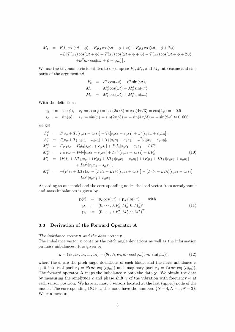
Mz = F1l1 cos(ωt+ φ) + F2l2 cos(ωt+ φ+ ϕ) + F3l3 cos(ωt+ φ+ 2ϕ)

+L [T (x1) cos(ωt+ φ) + T (x2) cos(ωt+ φ+ ϕ) + T (x3) cos(ωt+ φ+ 2ϕ)

+ω2mr cos(ωt+ φ+ φm)]

.

We use the trigonometric identities to decompose Fz,Mx, and Mz into cosine and sineparts of the argument ωt:

Fz = F cz cos(ωt) + F s

z sin(ωt),

Mx = M cx cos(ωt) +M s

x sin(ωt),

Mz = M cz cos(ωt) +M s

z sin(ωt)

With the definitions

cφ := cos(φ), c1 := cos(ϕ) = cos(2π/3) = cos(4π/3) = cos(2ϕ) = −0.5

sφ := sin(φ), s1 := sin(ϕ) = sin(2π/3) = − sin(4π/3) = − sin(2ϕ) ≈ 0, 866,

we get

F cz = T1sφ + T2[sφc1 + cφs1] + T3[sφc1 − cφs1] + ω2[sφx4 + cφx5],

F sz = T1cφ + T2[cφc1 − sφs1] + T3[cφc1 + sφs1] + ω2[cφx4 − sφx5],

M cx = F1l1sφ + F2l2[sφc1 + cφs1] + F3l3[sφc1 − cφs1] + LF c

z ,

M sx = F1l1cφ + F2l2[cφc1 − sφs1] + F3l3[cφc1 + sφs1] + LF s

z , (10)

M cz = (F1l1 + LT1)cφ + (F2l2 + LT2)[cφc1 − sφs1] + (F3l3 + LT3)[cφc1 + sφs1]

+ Lω2[cφx4 − sφx5],

M sz = −(F1l1 + LT1)sφ − (F2l2 + LT2)[sφc1 + cφs1]− (F3l3 + LT3)[sφc1 − cφs1]

− Lω2[sφx4 + cφx5].

According to our model and the corresponding nodes the load vector from aerodynamicand mass imbalances is given by

p(t) = pc cos(ωt) + ps sin(ωt) with

pc := (0, · · · , 0, F cz ,M

cx, 0,M

cz )

T (11)

ps := (0, · · · , 0, F sz ,M

sx, 0,M

sz )

T .

3.3 Derivation of the Forward Operator A

The imbalance vector x and the data vector yThe imbalance vector x contains the pitch angle deviations as well as the informationon mass imbalances. It is given by

x = (x1, x2, x3, x4, x5) = (θ1, θ2, θ3,mr cos(φm),mr sin(φm)), (12)

where the θi are the pitch angle deviations of each blade, and the mass imbalance issplit into real part x4 = ℜ(mr exp(iφm)) and imaginary part x5 = ℑ(mr exp(iφm)).The forward operator A maps the imbalance x onto the data y. We obtain the databy measuring the amplitude c and phase shift γ of the vibration with frequency ω ateach sensor position. We have at most 3 sensors located at the last (upper) node of themodel. The corresponding DOF at this node have the numbers N − 4, N − 3, N − 2.We can measure

8

1. the vibration cy(x) cos(ωt−γy(x)) at DOF (N −4) (displacement in y-direction),

2. the vibration cz(x) cos(ωt−γz(x)) at DOF (N −3) (displacement in z-direction),

3. the vibration cβx(x) cos(ωt−γβx

(x)) at DOF (N−2) (torsion around the x-axis).

For all vibrations we record the cosine and sine part of the vibration, cf. (13). Using

c cos (ωt− γ) = c cos(γ) cos(ωt) + c sin(γ) sin(ωt), (13)

we can arrange the data vector as

y =

cy(x) cos(γy(x))cz(x) cos(γz(x))cβx

(x) cos(γβx(x))

cy(x) sin(γy(x))cz(x) sin(γz(x))cβx

(x) sin(γβx(x))

,

for all three sensors.

3.3.1 Solution of the ODE system

In order to describe the operator A that maps the vector of imbalance x onto the datay we solve (1) for the cosine and the sine part of p, cf. (11), separately. The solutionu is the sum of the solutions uc and us of the two inhomogeneous systems

Muc(t) + Suc(t) = pc(x) cos(ωt),

Mus(t) + Sus(t) = ps(x) sin(ωt).

Although we have neglected the damping in the model of the WT, there will always besome small damping in every system. Therefore the homogenous solution is decaying.As the vibration data are obtained over a long time period, we can assume that thehomogenous solution has already died away. With the abbreviation

B := (−ω2M+ S)−1

the solutions are given by

uc(t) = Bpc cos(ωt),

us(t) = Bps sin(ωt).

with pc and ps from (11). Since both vectors pc and ps have only entries at the positions(N−3), (N−2), N and u(t) can only be measured at DOF (N−4), (N−3), (N−2),we restrict B,pc,ps, and u by withdrawing the relevant rows and columns (subscriptr, see (15)) and get

ur(t) = (Br pc,r) cos(ωt) + (Br ps,r) sin(ωt).

9

It follows that A is given by

A(x) = y =

(

Brpc,r

Brpc,s

)

(14)

where

pc,r(x) :=

F cz

M cx,

M cz

, ps,r(x) :=

F sz

M sx,

M sz

, and Br := B[N−4:N−2]; [N−3,N−2,N ].(15)

3.4 Derivative

We recall that parts of pc,r and ps,r occurring in the operator A are derived with thenonlinear BEM method. Hence A is a nonlinear operator. The Frechet derivative A′

of A is given by the Jacobi matrix

A′(x) =

(

Br

Br

)

(

∂pc,r

∂x1· · · ∂pc,r

∂x5

∂ps,r

∂x1· · · ∂ps,r

∂x5

)

, (16)

with

∂pc,r

∂xi=

∂F cz

∂xi∂Mc

x

∂xi∂Mc

z

∂xi

,

∂ps,r

∂xi=

∂F sz

∂xi∂Ms

x

∂xi∂Ms

z

∂xi

.

We denote by ∂Ti the partial derivative ∂Ti/∂xi and by ∂(Fl)i the partial derivative∂(Fi · li)/∂xi. Starting from (10) we have, e.g.

∂F cz

∂x1= sφ∂T1,

∂F cz

∂x2= (sφc1 + cφs1)∂T2,

∂F cz

∂x3= (sφc1 − cφs1)∂T3,

∂F cz

∂x4= ω2sφ,

∂F cz

∂x5= ω2cφ,

∂M cx

∂x1= sφ(∂(Fl)1 + L∂T1),

∂M cx

∂x2= (sφc1 + cφs1)(∂(Fl)2 + L∂T2), · · ·

It remains to compute the partial derivatives ∂Ti and ∂(Fl)i, i = 1, 2, 3. Since T, F,and l are obtained via a nonlinear numerical routine we cannot compute the partialderivatives explicitly. Instead, we use the differential quotients as an approximationprovided ∆ is small, e.g.

∂Tj

∂xj(xj) ≈ Tj((xj +∆)− Tj(xj)

∆, · · ·

∂(Fjlj)

∂xj(xj) ≈ ∂Fj

∂xj(xj)lj + Fj

∂lj∂xj

(xj), j = 1, 2, 3.

Numerical experiments show, that ∆ ≈ 0.1 provides a sufficiently accurate approxima-tion of the partial derivatives. Thus, the matrix

∂p =

(

∂pc,r

∂x1· · · ∂pc,r

∂x5

∂ps,r

∂x1· · · ∂ps,r

∂x5

)

(17)

can be computed.

10

4 Regularization

The inverse problem of (14) is to find the imbalance vector x for given data y that, incase of real measurements, are contaminated by noise. We assume that the noisy datayδ fulfill the inequality ‖y−yδ‖ ≤ δ, i.e., a bound on the noise is known. The operatorA is nonlinear and ill-posed. To obtain a stable solution, one has to use regularizationmethods, [6, 9]. Theoretical results for the regularization of nonlinear problems werederived in the last decade, cf. [11],[20]. We have used the most prominent Tikhonovregularization.

Tikhonov functional

In Tikhonov regularization we determine an approximation xδα of the solution x as a

minimizer of the Tikhonov functional Jα(x) with a rule to choose the regularizationparameter α. We use Morozovs discrepancy principle, i.e., we define a sequence of αk,e.g., αk+1 = qαk, q < 1, and compute xδ

αkas minimizer of Jαk

(x) for each k and stopthe iteration if for the first time

‖A(xδαk)− yδ‖ ≤ τδ, τ > 1 fixed,

holds. In order to minimize the Tikhonov functional for each αk we will use a gradient-based method. The Tikhonov functional is given by

Jα(x) = ‖A(x)− yδ‖2 + α‖x− x‖2,

where ‖ · ‖ is the usual l2(n)-norm with n = 5, and x is an a priori guess of thesolution. In our case, x can be the vector (0, 0, 0, mr cos(ϕm), mr sin(ϕm)) where themass imbalance is computed using MIA. In view of the different absolute values of theentries in the vector x it is appropriate to choose a weighted norm instead of ‖x− x‖2.According to the common applications we chose c = (1, 1, 1, 0.01, 0.01) and define

‖x‖2c :=5∑

i=1

cix2i = (c. ∗ x)Tx, ,

〈x, z〉c :=

5∑

i=1

cixizi = (c. ∗ x)T z,

where c. ∗ x = (c1x1, · · · , c5x5)T denotes the component-by-component multiplication.We remark that 〈x, z〉c = 〈c. ∗ x, z〉.Hence the Tikhonov functional now reads

Jα(x) = ‖A(x)− yδ‖2 + α‖x− x‖2c= ‖A(x)− yδ‖2 + α‖c. ∗ (x− x)‖2. (18)

4.1 The gradient of Tikhonov functional

In order to minimize the functional, the gradient has to be computed. Since A isnonlinear we use the Taylor expansion of A(x+ h),

A(x+ h) = A(x) +A′(x)h+O(h2),

11

where A′ is the Frechet derivative of A computed in (16) and (17). We have

Jα(x+ h) = ‖A(x)− yδ‖2 + α‖x− x‖2c+2〈1./c. ∗ [A′(x)]T (A(x)− yδ)+ α(x− x),h〉c +O(h2)

= Jα(x) + 2〈[A′(x)]T (A(x)− yδ) + α(c. ∗ (x− x)),h〉+O(h2).

It follows that

1

2 Jα(x) = 1./c. ∗ [A′(x)]T (A(x)− yδ)+ α(x− x)

= [A′(x)]T (A(x)− yδ) + αc. ∗ (x− x).

Minimization with steepest decent and algorithm

The functional (18) can be minimized for each fixed α by the steepest decent method.Starting from an initial value x0 the minimizer is is computed iteratively by updatingthe current iterate in the direction of steepest descent, i.e., the direction of the negativegradient:

xk+1 = xk − β Jα(x)

= xk + β2[A′(xk)]∗(yδ −A(xk))− αc. ∗ (xk − x).

There are theoretical results on how to choose the step size β, [6, 18]. In the numericalrealization, we have chosen β = 1/(2α2). If α becomes very small, β is chosen fixed,e.g. β = 10. The final minimization algorithm is as follows:

Algorithm 1

CHOOSEα, q < 1, τ > 1, x0, estimate δWHILE ‖A(x)− yδ‖ > τδ

α = qα, β = 12α2

if β > 10 then β = 10 endWHILE |Jα(x0)−Jα(x1)|

|Jα(x0)|> ε

Compute A′(x0)x1 = x0 + β2[A′(x0)]

∗(yδ −A(x0))− αc. ∗ (x0 − x)x0 = x1

endend

5 Numerical tests

5.1 Settings

Settings

Model dataWe have tested the imbalance reconstruction algorithm for a wind turbine of the type

12

NTK 500 with constant rotational frequency, since the aerodynamic data for this WTcan be found in the literature. Namely, we use the following system parameters:

• Rotational speed Ωrot = 0.45 Hz = 27 rpm

• Aerodynamic data: NACA63-421(lift and drag coefficients:http://airfoiltools.com/airfoil/details?airfoil=naca634421-il), NKT500-41(profiledata:http://www.readbag.com/130-226-17-201-extra-web-docs-nordtank-wt-description),blade length= 20.5 m, wind speed = 8 m/s

• Model data:

– Masses: mr = 9030 kg (rotor), mn = 15400 kg (nacelle), mt = 22500 kg(tower);

– Geometry: Tower height: h = 33.8 m, outer diameter at tower top: dtopout =1.69 m, outer diameter at tower bottom: dbotout = 2.4 m, distance from rotorto nacelle midpoint L = 1.5 m;

– Eigenfrequency: Ω0 = 0.925 Hz

We have set the zero mark at blade A. Thus blade B correspond to an angle of 240

and blade C corresponds to 120, resp. For example, assuming a pitch angle deviationof blade B of 2 compared to blade A and C and a mass imbalance of 50 kgm atblade A, the corresponding imbalance vector is x = (0, 2, 0, 50, 0)T ; if the imbalance isat blade C, we have x = (0, 2, 0, 50 cos(2/3π), 50 sin(2/3π))T . We obtain radial, axialand torsion vibration data y by applying the forward operator to x. To simulate realmeasurements, the data y is contaminated with gaussian noise. The disturbed data yδ

as well as the noise δ = ‖y−yδ‖ are used as input data for the reconstruction process.

Reconstruction qualityDue to the different magnitudes of mass imbalance and pitch angle deviation we haveto choose an appropriate metric in order to evaluate the reconstruction quality of ourmethod. Additionally, we observe that classes of pitch angle vectors actually representthe same pitch angle deviation, namely

(x1, x2, x3) ∼ (x1 + s, x2 + s, x3 + s), s ∈ R.

In order to obtain accuracy results we chose from the class of the reconstructed pitchangle deviation the representative (xδα,1+s, xδα,2+s, xδα,3+s) with the smallest distanceto the original pitch angle deviation (x1, x2, x3), i.e. we chose s s.t.

s = argmint∈R

‖(x1, x2, x3)− (xδα,1 + t, xδα,2 + t, xδα,3 + t)‖2.

As one can easily verify s is given by

s =1

3[(x1 − xδα,1) + (x2 − xδα,2) + (x3 − xδα,3)]. (19)

In practice the original pitch angle deviation is not known. Here we chose the numbers in a way that at least one of the xi, i = 1, 2, 3, is zero. The residual vibrations are

13

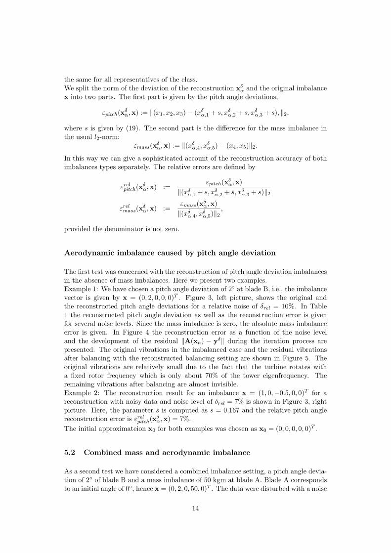
the same for all representatives of the class.We split the norm of the deviation of the reconstruction xδ

α and the original imbalancex into two parts. The first part is given by the pitch angle deviations,

εpitch(xδα,x) := ‖(x1, x2, x3)− (xδα,1 + s, xδα,2 + s, xδα,3 + s), ‖2,

where s is given by (19). The second part is the difference for the mass imbalance inthe usual l2-norm:

εmass(xδα,x) := ‖(xδα,4, xδα,5)− (x4, x5)‖2.

In this way we can give a sophisticated account of the reconstruction accuracy of bothimbalances types separately. The relative errors are defined by

εrelpitch(xδα,x) :=

εpitch(xδα,x)

‖(xδα,1 + s, xδα,2 + s, xδα,3 + s)‖2

εrelmass(xδα,x) :=

εmass(xδα,x)

‖(xδα,4, xδα,5)‖2,

provided the denominator is not zero.

Aerodynamic imbalance caused by pitch angle deviation

The first test was concerned with the reconstruction of pitch angle deviation imbalancesin the absence of mass imbalances. Here we present two examples.Example 1: We have chosen a pitch angle deviation of 2 at blade B, i.e., the imbalancevector is given by x = (0, 2, 0, 0, 0)T . Figure 3, left picture, shows the original andthe reconstructed pitch angle deviations for a relative noise of δrel = 10%. In Table1 the reconstructed pitch angle deviation as well as the reconstruction error is givenfor several noise levels. Since the mass imbalance is zero, the absolute mass imbalanceerror is given. In Figure 4 the reconstruction error as a function of the noise leveland the development of the residual ‖A(xn) − yδ‖ during the iteration process arepresented. The original vibrations in the imbalanced case and the residual vibrationsafter balancing with the reconstructed balancing setting are shown in Figure 5. Theoriginal vibrations are relatively small due to the fact that the turbine rotates witha fixed rotor frequency which is only about 70% of the tower eigenfrequency. Theremaining vibrations after balancing are almost invisible.Example 2: The reconstruction result for an imbalance x = (1, 0,−0.5, 0, 0)T for areconstruction with noisy data and noise level of δrel = 7% is shown in Figure 3, rightpicture. Here, the parameter s is computed as s = 0.167 and the relative pitch anglereconstruction error is εrelpitch(x

δα,x) = 7%.

The initial approximateion x0 for both examples was chosen as x0 = (0, 0, 0, 0, 0)T .

5.2 Combined mass and aerodynamic imbalance

As a second test we have considered a combined imbalance setting, a pitch angle devia-tion of 2 of blade B and a mass imbalance of 50 kgm at blade A. Blade A correspondsto an initial angle of 0, hence x = (0, 2, 0, 50, 0)T . The data were disturbed with a noise

14

Figure 3: Comparison of reconstruction and original pitch angle deviation; left picture:(0, 2, 0, 0, 0) with 10% noise level; right picture:(1, 0,−0.5, 0, 0) with 7% noise level

Table 1: Reconstruction results for imbalance x = (0, 2, 0, 0, 0)T

δrel s xδα .+ s εrelpitch(x

δα,x) εmass(x

δα,x)

3% 0.67 (−0.03, 1.93,−0.05, 0.04,−0.06)T 5.9 % 0.07

5% 0.67 ( 0.06, 1.97,−0.04, 0.03,−0.05)T 4.6 % 0.07

8% 0.67 ( 0.10, 1.94,−0.04, 0.04,−0.05)T 8.5 % 0.06

10% 0.67 (−0.06, 1.89, 0.16, 0.04,−0.05)T 13.2 % 0.06

12% 0.67 (−0.06, 1.88, 0.18, 0.02,−0.06)T 15 % 0.07

15% 0.67 ( 0.25, 1.82,−0.07, 0.02,−0.06)T 21.5 % 0.07

17% 0.67 (−0.09, 1.83, 0.25, 0.03,−0.06)T 21.7 % 0.07

Figure 4: Reconstruction error versus Noise level (left picture), Residua during iteration(right picture)

Figure 5: Imbalance vibrations and residual vibrations after balancing

15

was far too slow for extensive test computations. Also convergence was not always beachieved. With our gradient-based reconstruction method the computation time wasreduced significantly to a more reasonable time of about 2 minutes on 2.8 GHz IntelCore2 Duo processor. Convergence could also be observed in all tests.

6 Summary and outlook

The paper deals with the mathematical determination of two types of imbalances ina WT: aerodynamic imbalances from pitch angle deviation of the blades and massimbalances of the rotor. Presently, both types have to be determined on-site by anexpert team performing time consuming measurement procedures. The mathematicalapproach provides a reconstruction method that can be implemented into a conditionmonitoring system. Instead of the expert team, the method requires the knowledge ofgeometrical and physical parameters of the WT and aerodynamic airfoil data of theblades. Whereas the former usually can be obtained from inspection reports, the latterrepresent very sensible data and are hardly available for newer WT. For that reason, sofar the method could only be tested for an older NTK500 turbine. Unfortunately, ourindustrial partners could not provide the necessary vibration data for this type. Thuswe had to restrict all tests to artificial data. For future applicability, the WT ownersand manufacturers need to be persuaded that tit in beneficial for the safe operation ofthe turbine to provide the sensible airfoil data in a confined way.The problem of imbalance determination was addressed by the authors in former pa-pers. In this paper we have presented an improved algorithm to reconstruct massimbalance and pitch angle deviation of the rotor of a WT at the same time. Includingpitch angle deviations into the reconstruction leads to a nonlinear forward operator.The regularization of the inverse problem requires the minimization of the Tikhonovfunctional. Straight forward direct search method proved to be to slow and not stableenough for our purpose. Hence we employed gradient based minimization methods. Tothat end, we have derived the Frechet derivative of the forward operator that occursin the gradient of the Tikhonov functional. The accelerated algorithm was successfullyapplied to several test examples with artificial vibration data. In case of real vibra-tion data we expect equally good reconstruction results as in the test computations,provided that the necessary aerodynamic data of the blades are available.

References

[1] A. Donth, A. Grunwald, Ch. Heilmann, M. Melsheimer, Improving Performance ofWind Turbines through Blade Angle Optimisation and Rotor Balancing. EWEA2011, O&M strategies, PO.ID 350

[2] Caselitz, P.; Giebhardt, J., Rotor Condition Monitoring for Improved OperationalSafety of Offshore Wind Energy Converters. ASME Journal of Solar Energy Engi-neering, 2005, 127, 253-261.

[3] Hameed, Z., Hong, Y. S., Cho, Y. M., Ahn, S. H., Song, C- K., Condition monitoringand fault detection of wind turbines and related algorithms: A review. Renewableand Sustainable Energy Reviews. 13, 2009, pp. 1-39.

17

[4] Ramlau, R,; Niebsch, J., Imbalance Estimation Without Test Masses for WindTurbines. ASME Journal of Solar Energy Engineering, 2009, 131(1), 011010-1-011010-7.

[5] Niebsch, J., Ramlau, R., Nguyen, T. T., Mass and Aerodynamic imbalance Esti-mates of Wind Turbines. Energies, 2010, 3, 696-710.

[6] Engl, H. W.; Hanke, M.; Neubauer, A., Regularization of Inverse Problems; Kluwer:Dortrecht, 1996.

[7] Gasch, R.; Knothe, K. Strukturdynamik 2; Springer: Berlin, 1989.

[8] Hau, E. Wind Turbines: Fundamentals, Technologies, Application, Economics;Springer: Berlin, Heidelberg, 2006.

[9] Louis, A. K., Inverse und schlecht gestellte Probleme. Teubner, Stuttgart, 1989.

[10] Hansen, M. Aerodynamics of Wind Turbines; Earthscan: London, 2008.

[11] Kaltenbacher, B.; Neubauer, A.; Scherzer, O. Iterative Regularization Methods forNonlinear Ill-Posed Problems; Walter de Gruyter: Berlin, New York, 2008.

[12] Ingram, G. Wind Turbine Blade Analysis using the Blade Element MomentumMethod. Note on the BEM method, Durham University: Durham, 2005.

[13] Ahlstrom,A. Aeroelastic Simulations of Wind Turbine Dynamics,Royal Instituteof Technology, Department of Mechanics, Stockholm, 2005.

[14] Heuser, H. T Gewohnliche Differentialgleichungen; B. G. Teubner: Stuttgart, 1991.

[15] Ramlau, R. Morozov’s Discrepancy Principle for Tikhonov regularization of non-linear operators. Numerical Functional Analalysis and Optimization 2002, 23(1&2),147-172.

[16] Scherzer, O. Morozov’s Discrepancy Principle for Tikhonov regularization of non-linear operators. Computing 1993, 51, 45-60.

[17] Ramlau, R. A steepest descent algorithm for the global minimization of theTikhonov– functional. Inverse Problems 2002, 18(2), 381-405.

[18] R. Ramlau. TIGRA - an iterative algorithm for regularizing nonlinear illposedproblems. Inverse Problems, 2003, 19(2), 433 - 467.

[19] Ramlau, R. On the use of fixed point iterations for the regularization of nonlinearill-posed problems. Journal for Inverse and Ill-Posed Problems 2005, 13(2), 175-200.

[20] Ramlau, R.; Teschke, G. Tikhonov Replacement Functionals for Iteratively SolvingNonlinear Operator Equations. Inverse Problems 2005, 21(5), 1571-1592.

18