1

SIMULTANEOUS INVERSION OF SPECTRALLY-BROADENED 3D SEISMIC DATA: CASE STUDY FOR OLMOS UNCONVENTIONAL PLAY, SOUTH TEXAS

Gisela Porfiri1, John P. Castagna

2, Bruce M. Moriarty

3, Robert R. Stewart

4

1Lumina Geophysical,

formerly Swift Energy. g_porfiri@hotmail.com

2Lumina Geophysical. john.castagna@luminageo.com

3Swift Energy. bruce.moriarty@swiftenergy.com

4University of Houston. rrstewart@uh.edu

Keywords: simultaneous inversion, P-impedance, sweet spots, unconventional, high- resolution seismic. Resumen: Inversión simultanea de sísmica 3D de alta resolución: caso de estudio para el reservorio no convencional de la Formación Olmos, Sur de Texas El objetivo principal de este trabajo consiste en identificar sweet spots del reservorio no convencional de la Formación Olmos a partir de la inversión simultánea de sísmica pre-stack. El segundo objetivo consiste en la comparación de datos sísmicos originales vs. datos sísmicos de alta resolución. La sísmica de alta resolución es el producto de un proceso denominado sparse-layer inversion, que utiliza descomposición espectral para detectar patrones de interferencia variables en tiempo e invierte estos espectros de frecuencia locales con el fin de detectar y resolver intervalos delgados que se hallan por debajo de la resolución sísmica. La inversión simultánea es un proceso que genera volúmenes de Impedancia P, Impedancia S, y Densidad al mismo tiempo. El volumen de Impedancia P generado a partir de los datos sísmicos originales carece de la resolución vertical necesaria para detectar las capas delgadas que se hallan dentro del intervalo productivo de la Formación Olmos. Para resolver esta dificultad se incorporaron los datos sísmicos de alta resolución. En el volumen de Impedancia P generado a partir de la inversión sísmica de los datos de alta resolución se puede detectar una nueva anomalía con bajos valores de impedancia al suroeste del área de estudio. Esta nueva anomalía se correlaciona con las capas delgadas de alta porosidad que han sido interpretadas como la principal fuente de hidrocarburos. El proceso de inversión espectral aplicado a la sísmica mejoró la resolución vertical de 37 a 18 metros. A su vez, la interpretación de estos datos permitió la identificación de dos horizontes adicionales dentro del intervalo productivo de Olmos. INTRODUCTION In South Texas, tight gas sandstone reservoirs in the Olmos Formation are prospective. Unfortunately, detecting and mapping the lateral continuity of reservoir quality Olmos sands is limited by the fact that prospective pay zones are commonly below conventional seismic resolution. Thus, spectral broadening is potentially valuable if it can be shown to be useful in this area. This paper describes seismic interpretation and simultaneous inversion results of an original and a spectrally-broadened high-resolution seismic dataset across the South Texas Olmos tight sand. The incorporation of high-resolution seismic data addresses the lack of enough vertical resolution to image thin beds within the Olmos productive zone. This high-resolution seismic data results from the application of the sparse-layer inversion method (Zhang and Castagna 2011) to the original pre-stack seismic data. The method is unbiased against thin beds and thus allows the detection and resolution of thin beds below tuning thickness. In this study, we found that inverted, low P-impedance intervals in the Olmos Formation are correlated to high production values; therefore, low P-impedance zone recognition is essential for sweet spots or productive-prone zone (PPZ) identification. The main goal is to use pre-stack seismic data and the high-resolution seismic gathers to generate simultaneously seismic inverted volumes to characterize the physical response of those low-

2

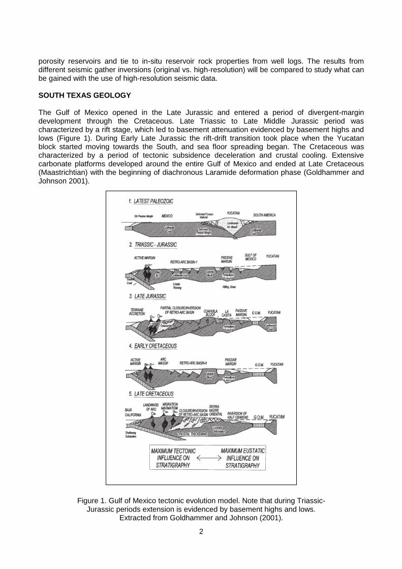
porosity reservoirs and tie to in-situ reservoir rock properties from well logs. The results from different seismic gather inversions (original vs. high-resolution) will be compared to study what can be gained with the use of high-resolution seismic data. SOUTH TEXAS GEOLOGY The Gulf of Mexico opened in the Late Jurassic and entered a period of divergent-margin development through the Cretaceous. Late Triassic to Late Middle Jurassic period was characterized by a rift stage, which led to basement attenuation evidenced by basement highs and lows (Figure 1). During Early Late Jurassic the rift-drift transition took place when the Yucatan block started moving towards the South, and sea floor spreading began. The Cretaceous was characterized by a period of tectonic subsidence deceleration and crustal cooling. Extensive carbonate platforms developed around the entire Gulf of Mexico and ended at Late Cretaceous (Maastrichtian) with the beginning of diachronous Laramide deformation phase (Goldhammer and Johnson 2001).

Figure 1. Gulf of Mexico tectonic evolution model. Note that during Triassic-Jurassic periods extension is evidenced by basement highs and lows.

Extracted from Goldhammer and Johnson (2001).

3

The Cretaceous succession of South Texas is interpreted as one first-order (200-400 Myr) transgressive-regressive sedimentary cycle, in which the stratigraphic evolution was dominated by relative sea-level changes. The Lower Cretaceous succession can be divided in two transgressive-regressive second-order sedimentary cycles. Each regressive cycle during Early Cretaceous is characterized by reef development along the break between the continental shelf and the Gulf of Mexico basin. These two episodes of reef formation are: 1) Sligo (Hauterivian to Barremian) and 2) Edwards or Stuart City (Albian) which is the younger episode and generally occurred in a more inland-ward position than the Sligo. In many areas of the Gulf of Mexico the Edwards margin prograded towards the Sligo margin leading to a sharp physiographic edge between the continental shelf and continental slope at the end of Early Cretaceous. In South Texas the situation was different, the Edwards margin prograded towards the continent resulting in a two-step complex continental margin at the end of Early Cretaceous (Figure 2) (Condon and Dyman 2006; Donovan and Staerker 2010). Late Cretaceous was characterized by a marine transgression in which lime, mudstones and shales were deposited. In South Texas, the succession is composed by the following lithostratigraphic units (from older to younger): Del Rio, Buda, Eagle Ford, Austin, Anacacho, San Miguel, Olmos and Escondido (Figure 3). This study focuses on the Olmos Formation thus only the lithologic and depositional characteristics for this Formation will be summarized.

Figure 2. Map of Texas showing the position of Sligo and Edwards Paleo-margins. Note the red square pointing the study area location. Modified from Donovan and Staerker (2010).

4

Olmos deposits consists in deltaic sands that prograded from the North-West and accumulated along the shelf margin as a response to a significant relative sea level fall during Upper Cretaceous (lower Maastrichtian). Submarine gravity flows developed on the shelf, slope and basin plain and led to turbidite flow deposition. There are two interpretations of the Olmos sandstone deposition, and both agreed in that it was deposited under a deltaic regime. According to Dennis (1987), Olmos deposition is interpreted as a delta-fed submarine ramp depositional model because there is no evidence of a major canyon existence in the seismic data of the area. On this model, the sedimentological components of the Olmos Formation consist of: 1) sandy deltaic system that prograded to the shelf-slope break; 2) pro-delta slope transversed by multiple shallow gullies; 3) proximal ramp deposits that resulted from high-density turbidite currents (Lowe 1982) or massive turbidite sandstone beds of Facies B (Ricci-Lucchi 1972); 4) distal ramp deposits resulted from low-density turbidite flows (Heller and Dickinson 1985; and Dennis 1987). During Olmos deposition there was a downthrown fault that acted as a plane of movement leading to

Figure 3. Lithostratigraphic column of eastern and southern Texas. The study area is represented by the Rio Grande Embayment region. The rock interval of interest (Olmos Formation) is highlighted in red. (Modified

from Condon and Dyman (2006)

5

slumping of the unstable delta front sediments deposited on the faulted area. At present, structural dip is North-West to South-East corresponding with the Paleo Golf of Mexico basin direction. Olmos sediment porosity and permeability decrease in a basinward direction due to an increase in clay content resulting from to the low-density turbidite flows deposited at the distal ramp (Dennis 1987). On the other hand, Tyler and Ambrose (1986) identified the lower Olmos as deposited in a deltaic system followed by a barrier/strandplain system. Trevino et al. (2007) analyzed cores from well logs and recognized channel related facies. They defined Olmos depositional system and evolution as a wave-dominated deltaic system that periodically prograded over the shoreface and was alternately transgressed by the shoreface deposits by autocyclic delta-lobe switching and abandonment. In this study the Olmos is interpreted as a deltaic system with a principal channel as a source of sediment. According to well data near the study area, channel facies were recognized to the North-East (Ann Gafford, personal communication). Olmos sediments correspond to laminated sands deposited in lower low energy shoreface-inner shelf environment intercalated with silts and shales accumulated by storm deposits. Longshore currents run parallel to the coastline towards the South-West transporting fine-grained sediments far away from the source. This led to the sand/shale proportion reduction towards the South-West where quieter water allowed fine sediments to settle. HIGH-RESOLUTION SEISMIC DATA AND INTERPRETATION The study area is located in the McMullen County (Figure 2), South Texas and comprises ~ 32 sq mi (83 sq km) region. The dataset includes full-azimuth, full-offset 3D seismic gathers with a sample interval of 3 ms and an offset of 26,000 ft (7925 m) (80 degrees angle offset), an RMS velocity model, and four wells with a suite of digital well logs. Many gather conditioning processes were applied to obtain final pre-stack seismic gathers converted from offset to angle (in which angles from 4 to 46 degrees were retained). Four gas and/or oil producing wells in the database have P-wave, S-wave, gamma ray, and density logs. Three out of the four wells are horizontal wells and the logs interpreted in this work correspond to the vertical pilot well. Two wells are producing from the Olmos Formation. Well log interpretation for the Olmos shows that Top and Base of the PPZ is delimited by low Density and high Shear (S) wave log values (Figure 4). The PPZ has an average thickness of 86 ft/ 26 m with a 107 ft/ 32.5 m maximum thickness in one of the wells. Seismic interpretation was done on the post-stack conditioned seismic volume. First, the wells were tied to seismic to study the seismic response at each marker and elaborate the time-depth charts (Figures 5 and 6). The seismic is American polarity, this means that a seismic peak (blue color) represents an increase in acoustic impedance and a seismic trough (red color) represents a decrease in acoustic impedance. Therefore, Olmos top of the PPZ is a seismic trough, which is expected due to the decrease in acoustic impedance. The base of the PPZ is the peak right below the Olmos trough (Figure 7). Olmos time thickness is consistent (~2ms) within the study area there are not significant thickness variations along the entire volume. A tuning chart generated for the interval of interest on the original seismic data shows that the maximum peak-to-trough amplitude occurs at 20 ms (TWT). This means that vertical resolution of the data at the interval of interest is 20 ms, which corresponds to a ~100 ft/ 30 m tuning thickness (based on the velocity extracted from RMS velocity model) (Figure 8). Therefore, the Olmos PPZ (107 ft/ 32.5 m maximum thickness) is about seismic resolution. However, the thin beds within the Olmos high-porosity interval cannot be resolved on the seismic. To improve seismic resolution, a sparse-layer inversion method developed by Zhang and Castagna (2011) was applied to the original seismic data. Said method uses a priori information and spectral decomposition to improve the resolution, but does not directly utilize well logs in a starting model. Thin beds below tuning thickness (i.e. maximum constructive interference that occurs when the bed thickness reaches one quarter of the wavelength at dominant frequency

6

(Kallweit and Wood 1982; Brown 2004)) can be imaged by inverting the frequency spectra for layer thickness using complex spectral analysis. The process was applied to five different partial angle stacks. As a result, high-resolution pre-stack seismic data containing five traces was obtained (12°, 20°, 27°, 35°, and 42° angle traces). The maximum peak-to-trough amplitude of this high-resolution seismic data occurs at 10 ms (TWT), when using a velocity model this translates to ~ 50 ft (15 m) of tuning thickness (Figure 8). The bandwidth extension process thus doubles the original data resolution. The frequency spectrum of high-resolution seismic shows that much higher frequencies were added to the seismic data when compared to the original. Consequently, two additional horizons are interpreted within the Olmos PPZ (Figure 7). These were the top and base of Olmos PPZ thin layers separated by shale breaks that could not be seen on the original seismic. This represents an important advantage since it could aid in the productive interval identification.

OLMOS PPZ

P-WAVE DENSITY S-WAVE GR AIVpVs

86 ft

(26.2 m)

Figure 4. The well logs display shows the interpretation of the Olmos productive prone zone (PPZ) at one of the wells in the study area. The P-wave, density, shear wave, and gamma ray

logs were registered while VpVs and acoustic impedance (AI) logs were calculated (highlighted with a yellow star). The Olmos productive interval is identified by low density log

values and shows a thickness of 86 ft/26m.

7

GAMMA WELL

Figure 5. Well-to-seismic tie at Gamma well using the original seismic. The upper left figure is the wavelet used to tie the well to the near stack. Correlation coefficient achieved is 0.725, and the correlation diagram (lower right figure) shows that wavelet and seismic

are both close to zero phase.

Figure 6. Near-offset well-to-seismic tie at Gamma well to the high-resolution seismic. The upper left figure is the wavelet used to tie the well to the near stack. Correlation coefficient achieved is 0.435, and the correlation diagram (lower right

figure) shows that wavelet and seismic are both zero phase.

GAMMA WELL

8

Figure 7. This figure shows the Olmos seismic interpretation on the original (left) and the high-resolution (right) seismic data along an arbitrary line at one of the horizontal wells (black line on the map). Note that two more horizons can be

interpreted within the Olmos PPZ in the high-resolution seismic besides Top and Base of the PPZ. Blue represents positive seismic amplitudes and red negative

seismic amplitudes.

20 ms

10 ms

Figure 8. Tuning analysis chart of original (left) and high-resolution (right) seismic data at the Olmos Formation interval. The upper panel shows the wavelet used for

the tuning analysis (extracted from original and high-resolution seismic data, respectively, on a time interval from 2 to 3 seconds), and the lower panel shows a

chart with the Normalized Peak-Trough Amplitude curve (red).

GR

DENSITY

SONICGR

DENSITY

SONIC

HIGH-RESOLUTIONORIGINAL SEISMIC

0.1 Km0.1 Km

BETA

GAMMA

DELTA

ALPHA

9

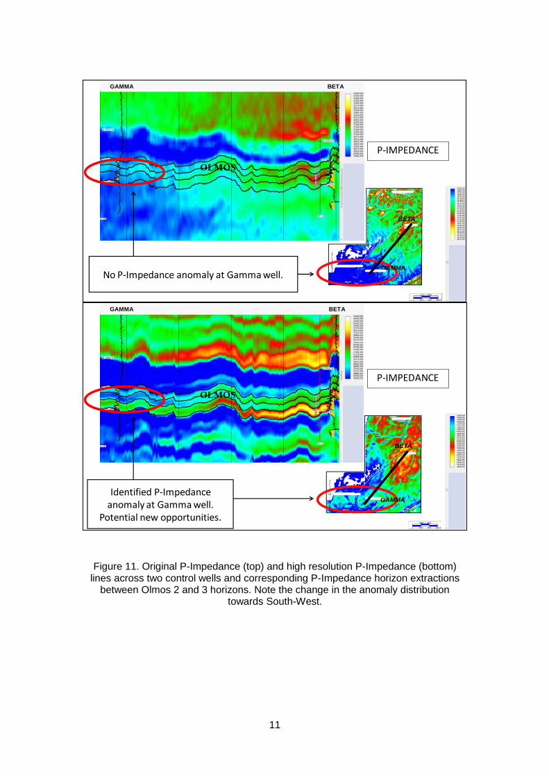
SIMULTANEOUS INVERSION AND ANALYSIS Acoustic properties can be derived from seismic data by means of seismic inversion processes. This allows the calculation of the impedance (velocity*density) for each layer from seismic amplitudes. Acoustic impedance can be calculated at the well location, and is the connection between well and seismic data (Latimer et al. 2000). Simultaneous inversion is one of the pre-stack seismic inversion processes in which P-impedance, S-impedance, and density volumes are created simultaneously. The method is based in three assumptions: 1) linearized approximation for reflectivity holds, 2) the Aki-Richards equation gives the reflectivity as a function of angle, and 3) there is, to first order, a linear relationship between P-impedance and both S-impedance and density (Gardner’s relationship: Δδ/δ=(1/4)(ΔVp/Vp), and Castagna’s equation: Vs=(Vp-1360)/1.16). Hampson-Russell software uses the AVO Equation (Fatti et al. 1994) that considers the P-reflectivity, S-reflectivity, a geometric factor (that includes the different incidence angles of the gather), and density reflectivity (Hampson and Russell 2005). The principal issue of this method is that the seismic input is band-limited, i.e. it has low and high cutoffs in the frequency spectra (Figure 9). The absolute impedance variations can be calculated by adding the missing low-frequencies. The solution to this consists in using a priori information (well logs and interpreted horizons) to build P-Impedance, S-Impedance and density initial band-limited low-frequency models. This a priori information permits the calculation of the impedance traces that tie to the well log information (Duboz et al. 1998). Then, by several iterations, using the conjugate gradient method, with the original seismic data the software generates an inverted trace which contains the low frequencies and the original frequency spectra of the input seismic (Figure 10). Simultaneous inversion workflow has many steps. First, wavelet needs to be estimated and tied to seismic for near, mid and far offsets separately. Separate offset gathers ties facilitate the compensation for offset dependant phase, bandwidth, tuning and NMO stretch effects (Pendrel et al. 2000). Wavelet estimation is extremely important since it is the link between seismic and rock properties seen on the well (White 1997). After that, the analysis process generates a local inversion at each well location. This allows finding the best relationships between P-impedance, S-impedance, and density. This set of parameters controls the background relationship, which is used to stabilize the inversion. In order to reduce the non-uniqueness, the following relationships are assumed to hold for the background wet trend: ln(Dn)= m ln(Zp) + mc and ln(Zs)= k ln(Zp) + kc (where the coefficients k, kc, m, and mc will be determined by analyzing well logs from the area) (Hampson and Russell 2005). Cross-plots of those properties (Zp, Zs, Density, and VpVs) at the well locations for the original and the inverted results aid in the parameter selection. Once the parameters of the relationships are successfully tested the data is ready to generate the inverted volumes. The objective of this work comprises simultaneous inversion of the original and the high resolution seismic data (best case scenario for each dataset). Then compare the volumes at the levels of interest and study any resolution improvement. The first inverted property to analyze is the P-Impedance. The workflow consisted in compare the P-Impedance changes along the cross-section trough the wells and horizon extraction maps, and between the original vs. high-resolution seismic inverted volumes. The P-Impedance volume resulting from the original seismic inversion shows anomalous low values on the North to North-East region (Figure 11). The cross-section shows low P-impedance values within the PPZ. The impedance range is 25,500-30,000 (ft/s)*(g/cc), with lower values (less than 28,000 (ft/s)*(g/cc)) at Beta well location. The analysis of the high-resolution seismic inversion shows that P-impedance decreases towards the South South-West region (Figure 11). Low P-impedance trends can be recognized in that area. Cross-section along the wells shows low values within the PPZ. The impedance range is 24,000-29,000 (ft/s)*(g/cc), with lower values (less than 25,500 (ft/s)*(g/cc)) at Beta well location. At Gamma well location, a new P-Impedance anomaly can be identified (Figure 11). The low impedance values correspond to the deeper thin layer identified on the high-resolution seismic. Thus, the high resolution process reveals prospective productive locations that are not apparent on a conventional seismic inversion.

10

Figure 9.Example of a seismic section and its frequency spectrum. The seismic data is band-limited, it exhibits low and high cutoffs. One problem in the inversion process is that it needs low frequencies.

Figure 10. Upper figure shows the original (blue), the filtered log (black), and the inverted result (red) for the P and S-Impedance and VpVs ratio at one of the well locations. Lower figure shows the frequency spectra for each log curve. Note that by filtering back the original well log the low frequencies can be recovered.

11

BETA

OLMOS

P-IMPEDANCE

Identified P-Impedance anomaly at Gamma well.

Potential new opportunities.

GAMMA

GAMMA BETA

Figure 11. Original P-Impedance (top) and high resolution P-Impedance (bottom) lines across two control wells and corresponding P-Impedance horizon extractions

between Olmos 2 and 3 horizons. Note the change in the anomaly distribution towards South-West.

BETA

OLMOS

P-IMPEDANCE

No P-Impedance anomaly at Gamma well.GAMMA

GAMMA BETA

12

CONCLUSIONS The sparse-layer high-resolution seismic vertical resolution is double that of the original seismic data based on frequency bandwidth; this is verified by well ties. As a result, tuning thickness was improved from 100 ft on the original seismic to less than 50 ft on the high-resolution seismic. This allowed the interpretation of additional horizons within the interval of interest in the high-resolution seismic data. Horizon extraction comparison between original vs. high-resolution inverted P-impedance of the PPZ shows different anomaly distribution in the Southwest region. A productive well, previously not associated with an impedance anomaly, is seen to consist of thin pays that were not previously resolved, but can be mapped on the high resolution data. Using the additional interpreted horizons allowed the localization of that low p-impedance layer within the PPZ. We conclude that high-resolution seismic inversion may allow better definition of productive zones in the Olmos formation. ACKNOWLEDGEMENTS The authors would like to thank Joseph Sonnier, and Scott Scholz (Swift Energy) for their invaluable time and contributions. The authors would also like to express their thanks to Swift Energy for their support, Global Geophysical for kindly granting permission to display this dataset, and Lumina Geophysical for processing the high resolution data used in this investigation. CITED REFERENCES Brown, A. R., 2004, Interpretation of Three-dimensional Seismic Data, 6th edition: AAPG Memoir 42. Castagna, J. P., and C. I. Puryear, 2008, Layer-thickness determination and stratigraphic interpretation using spectral inversion: Theory and application: Geophysics, 73, no.2, 37-48. Condon, S.M., and Dyman, T.S., 2006, 2003 geologic assessment of undiscovered conventional oil and gas resources in the Upper Cretaceous Navarro and Taylor Groups, Western Gulf Province, Texas: U.S. Geological Survey Digital Data Series DDS–69–H. Dennis, J. G., 1987, Depositional environments of the A.W. P. Olmos Field, McMullen County, Texas: Gulf Coast Association of Geological Societies Transactions, 37, 55-63. Donovan, A. D. and T. S. Staerker, 2010, Sequence stratigraphy of the Eagle Ford (Boquillas) Formation in the subsurface of South Texas and outcrops of West Texas: Gulf Coast association of Geological Societies Transactions, 60, 861- 899. Duboz, P., Y. Lafet, and D. Mougenot, 1998, Moving to a layered impedance cube: advantages of 3D stratigraphic inversion: First Break, 16, no.9, 311-318. Fatti J.,G. Smith, P. Vail, P. Strauss, and P. Levitt, 1994, Detection of gas in sandstone reservoirs using AVO analysis: A 3D seismic case history using the Geostack technique: Geophysics, 59, 1362-1376. Goldhammer, R.K. and C.A. Johnson, 2001, Middle Jurassic-Upper Cretaceous Paleogeographic evolution and sequence-stratigraphic framework of the Northwest Gulf of Mexico rim, in C. Bartolini, R.T. Buffler, and A. Cantu - Chapa, eds., The Western Gulf of Mexico Basin; Tectonics, Sedimentary Basins, and Petroleum Systems: AAPG Memoir 75, 45-81. Hampson, D. P., B. H. Russell, and B. Bankhead, 2005, Simultaneous inversion of pre-stack seismic data. 75th Annual International Meeting, SEG, Expanded Abstracts, 1633-1637. Heller P. L., and W. R. Dickinson, 1985, Submarine ramp facies model for delta-fed, sand-rich turbidite systems: American Association of Petroleum Geologists Bulletin, 69, 813-826. Kallweit, R. S., and L. C. Wood, 1982, The limits of resolution of zero-phase wavelets: Geophysics, 47, no.7, 1035–1046.

13

Latimer R. B., R. Davison, and P. van Riel, 2000, An interpreter’s guide to understanding and working with seismic-derived acoustic impedance data: The Leading Edge, 28, no.3, 242-256. Lowe, D.R., 1982. Sediment gravity flows: II. Depositional models with special reference to the deposits of high-density turbidity currents. Journal of Sedimentary Petrology, 52, 279– 297. Mutti, E. and F. Ricci Lucchi, 1972, Turbidites of the northern Apennines: Introduction to facies analysis: Memorie della Societa Geologica Italiana, 11, 161-199. Pendrel, J., H. Debeye, R. Pedersen, B. Goodway, J. Dufour, M. Bogaards, and R. R. Stewart, 2000, Estimation and interpretation of P and S impedance volumes from simultaneous inversion of Pwave offset seismic data: 70th Annual International Meeting, SEG, Expanded Abstracts, 146-149. Tyler, N., and W. A. Ambrose, 1986, Depositional systems and oil and gas plays in the Cretaceous Olmos Formation, South Texas: Texas Bureau of Economic Geology Report of Investigations, 152. White R., 1997, The accuracy of well ties: practical procedures and examples: 67th Annual International Meeting, SEG, Expanded Abstracts, 816-819. Zhang, R., and Castagna, J. P., 2011, Seismic sparse-layer reflectivity inversion using basis pursuit decomposition: Geophysics, 76, no.6, R147–R158.