single-agent dynamic optimization models 1 rust...
TRANSCRIPT

Lecture notes: single-agent dynamics 1
Single-agent dynamic optimization models
In these lecture notes we consider specification and estimation of dynamic optimiza-
tion models. Focus on single-agent models.
1 Rust (1987)
Rust (1987) is one of the first papers in this literature. Model is quite simple, but
empirical framework introduced in this paper for dynamic discrete-choice (DDC)
models is still widely applied.
Agent is Harold Zurcher, manager of bus depot in Madison, Wisconsin. Each week,
HZ must decide whether to replace the bus engine, or keep it running for another week.
This engine replacement problem is an example of an optimal stopping problem, which
features the usual tradeoff: (i) there are large fixed costs associated with “stopping”
(replacing the engine), but new engine has lower associated future maintenance costs;
(ii) by not replacing the engine, you avoid the fixed replacement costs, but suffer
higher future maintenance costs. Optimal solution is characterized by a threshold-
type of rule: there is a “critical” cutoff mileage level x∗ below which no replacement
takes place, but above which replacement will take place.
Remark: Another well-known example of optimal stopping problem in economics is
job search model: each period, unemployed worker decides whether to accept a job
offer, or continue searching. Optimal policy is characterized by “reservation wage”:
accept all job offers with wage above a certain threshold.
1.1 Behavioral Model
At the end of each week t, HZ decides whether or not to replace engine. Control
variable defined as:
it =
{
1 if HZ replaces
0 otherwise.
For simplicity. we describe the case where there is only one bus (in the paper, buses
are treated as independent entities).

Lecture notes: single-agent dynamics 2
HZ chooses the (infinite) sequence {i1, i2, i3, . . . , it, it+1, . . . } to maximize discounted
expected utility stream:
max{i1,i2,i3,... ,it,it+1,... }
E∞∑
t=1
βt−1u (xt, ǫt, it; θ) (1)
where
• xt is the mileage of the bus at the end of week t. Assume that evolution of
mileage is stochastic (from HZ’s point of view) and follows
xt+1
{
∼ G(x′|xt) if it = 0 (don’t replace engine in period t)
= 0 if it = 1: once replaced, bus is good as new(2)
and G(x′|x) is the conditional probability distribution of next period’s mileage
x′ given that current mileage is x. HZ knows G; econometrician knows the form
of G, up to a vector of parameters which are estimated.
• ǫt denotes shocks in period t, which affect HZ’s choice of whether to replace the
engine. These are the “structural errors” of the model (they are observed by
HZ, but not by us), and we will discuss them in more detail below.
• Since mileage evolves randomly, this implies that even given a sequence of
replacement choices {i1, i2, i3, . . . , it, it+1, . . . }, the corresponding sequence of
mileages {x1, x2, x3, . . . , xt, xt+1, . . . } is still random. The expectation in Eq.
(1) is over this stochastic sequence of mileages and over the shocks {ǫ1, ǫ2, . . . }.
• The state variables of this problem are:
1. xt: the mileage. Both HZ and the econometrician observe this, so we call
this the “observed state variable”
2. ǫt: the utility shocks. Econometrician does not observe this, so we call it
the “unobserved state variable”
Define value function:
V (xt, ǫt) = maxiτ , τ=t+1,t+2,...
Et
[∞∑
τ=t+1
βτ−tu (xt, ǫt, it; θ) |xt
]
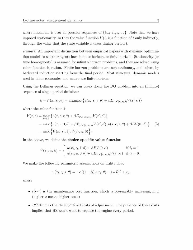
Lecture notes: single-agent dynamics 3
where maximum is over all possible sequences of {it+1, it+2, . . . }. Note that we have
imposed stationarity, so that the value function V (·) is a function of t only indirectly,
through the value that the state variable x takes during period t.
Remark: An important distinction between empirical papers with dynamic optimiza-
tion models is whether agents have infinite-horizon, or finite-horizon. Stationarity (or
time homogeneity) is assumed for infinite-horizon problems, and they are solved using
value function iteration. Finite-horizon problems are non-stationary, and solved by
backward induction starting from the final period. Most structural dynamic models
used in labor economics and macro are finite-horizon.
Using the Bellman equation, we can break down the DO problem into an (infinite)
sequence of single-period decisions:
it = i∗(xt, ǫt; θ) = argmaxi
{u(xt, ǫt, i; θ) + βEx′,ǫ′|xt,ǫt,itV (x′, ǫ′)
}
where the value function is
V (x, ǫ) = maxi=1,0
{u(x, ǫ, i; θ) + βEx′,ǫ′|xt,ǫt,itV (x′, ǫ′)
}
= max{u(x, ǫ, 0; θ) + βEx′,ǫ′|xt,ǫt,itV (x′, ǫ′), u(x, ǫ, 1; θ) + βEV (0, ǫ′).
}
= max{
V (xt, ǫt, 1), V (xt, ǫt, 0)}
.
(3)
In the above, we define the choice-specific value function
V (xt, ǫt, it) =
{
u(xt, ǫt, 1; θ) + βEV (0, ǫ′) if it = 1
u(xt, ǫt, 0; θ) + βEx′,ǫ′|xt,ǫt,itV (x′, ǫ′) if it = 0.
We make the following parametric assumptions on utility flow:
u(xt, ǫt, i; θ) = −c ((1 − it) ∗ xt; θ) − i ∗ RC + ǫit
where
• c(· · · ) is the maintenance cost function, which is presumably increasing in x
(higher x means higher costs)
• RC denotes the “lumpy” fixed costs of adjustment. The presence of these costs
implies that HZ won’t want to replace the engine every period.
Lecture notes: single-agent dynamics 4
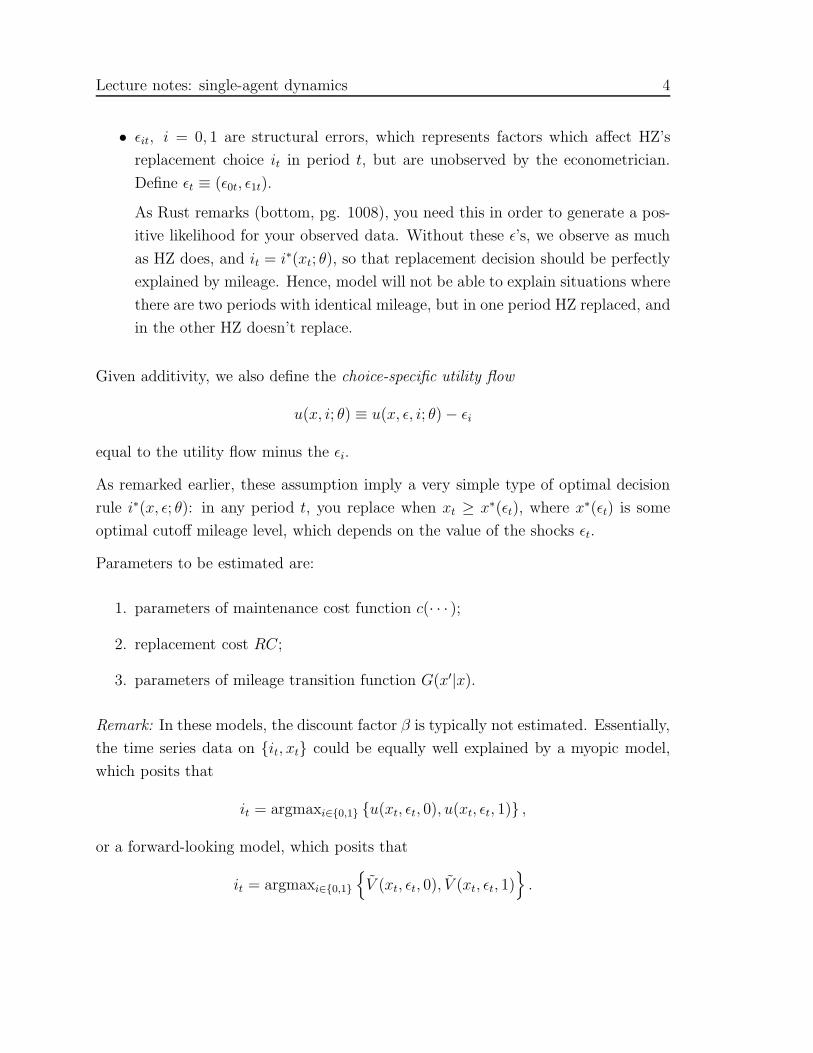
• ǫit, i = 0, 1 are structural errors, which represents factors which affect HZ’s
replacement choice it in period t, but are unobserved by the econometrician.
Define ǫt ≡ (ǫ0t, ǫ1t).
As Rust remarks (bottom, pg. 1008), you need this in order to generate a pos-
itive likelihood for your observed data. Without these ǫ’s, we observe as much
as HZ does, and it = i∗(xt; θ), so that replacement decision should be perfectly
explained by mileage. Hence, model will not be able to explain situations where
there are two periods with identical mileage, but in one period HZ replaced, and
in the other HZ doesn’t replace.
Given additivity, we also define the choice-specific utility flow
u(x, i; θ) ≡ u(x, ǫ, i; θ) − ǫi
equal to the utility flow minus the ǫi.
As remarked earlier, these assumption imply a very simple type of optimal decision
rule i∗(x, ǫ; θ): in any period t, you replace when xt ≥ x∗(ǫt), where x∗(ǫt) is some
optimal cutoff mileage level, which depends on the value of the shocks ǫt.
Parameters to be estimated are:
1. parameters of maintenance cost function c(· · · );
2. replacement cost RC;
3. parameters of mileage transition function G(x′|x).
Remark: In these models, the discount factor β is typically not estimated. Essentially,
the time series data on {it, xt} could be equally well explained by a myopic model,
which posits that
it = argmaxi∈{0,1} {u(xt, ǫt, 0), u(xt, ǫt, 1)} ,
or a forward-looking model, which posits that
it = argmaxi∈{0,1}
{
V (xt, ǫt, 0), V (xt, ǫt, 1)}
.

Lecture notes: single-agent dynamics 5
In both models, the choice it depends just on the current state variables xt, ǫt. Indeed,
Magnac and Thesmar (2002) shows that in general, DDC models are nonparamet-
rically underidentified, without knowledge of β and F (ǫ), the distribution of the
ǫ shocks. (Below, we show how knowledge of β and F , along with an additional
normalization, permits nonparametric identification of the utility functions in this
model.)
Intuitively, in this model, it is difficult to identify β apart from fixed costs. In this
model, if HZ were myopic (ie. β close to zero) and replacement costs RC were low, his
decisions may look similar as when he were forward-looking (ie. β close to 1) and RC
were large. Reduced-form tests for forward-looking behavior exploit scenarios in which
some variables which affect future utility are known in period t: consumers are deemed
forward-looking if their period t decisions depends on these variables. (Example:
Chevalier and Goolsbee (2005) examine whether students’ choices of purchasing a
textbook now depend on the possibility that a new edition will be released soon.)
1.2 Econometric Model
Data: observe {it, xt} , t = 1, . . . , T for 62 buses. Treat buses as homogeneous and
independent (ie. replacement decision on bus i is not affected by replacement decision
on bus j).
Rust makes the following conditional independence assumption, on the Markovian
transition probabilities in the Bellman equation above:
p(x′, ǫ′|x, ǫ, i) = p(ǫ′|x′, x, ǫ, i) · p(x′|x, e, i)
= p(ǫ′|x′) · p(x′|x, i).(4)
The first line is just factoring the joint density into a conditional times a marginal.
The second line shows the simplifications from Rust’s assumptions. Namely, two
types of conditional independence: (i) given x, ǫ’s are independent over time; and (ii)
conditional on x and i, x′ is independent of ǫ.
Lecture notes: single-agent dynamics 6
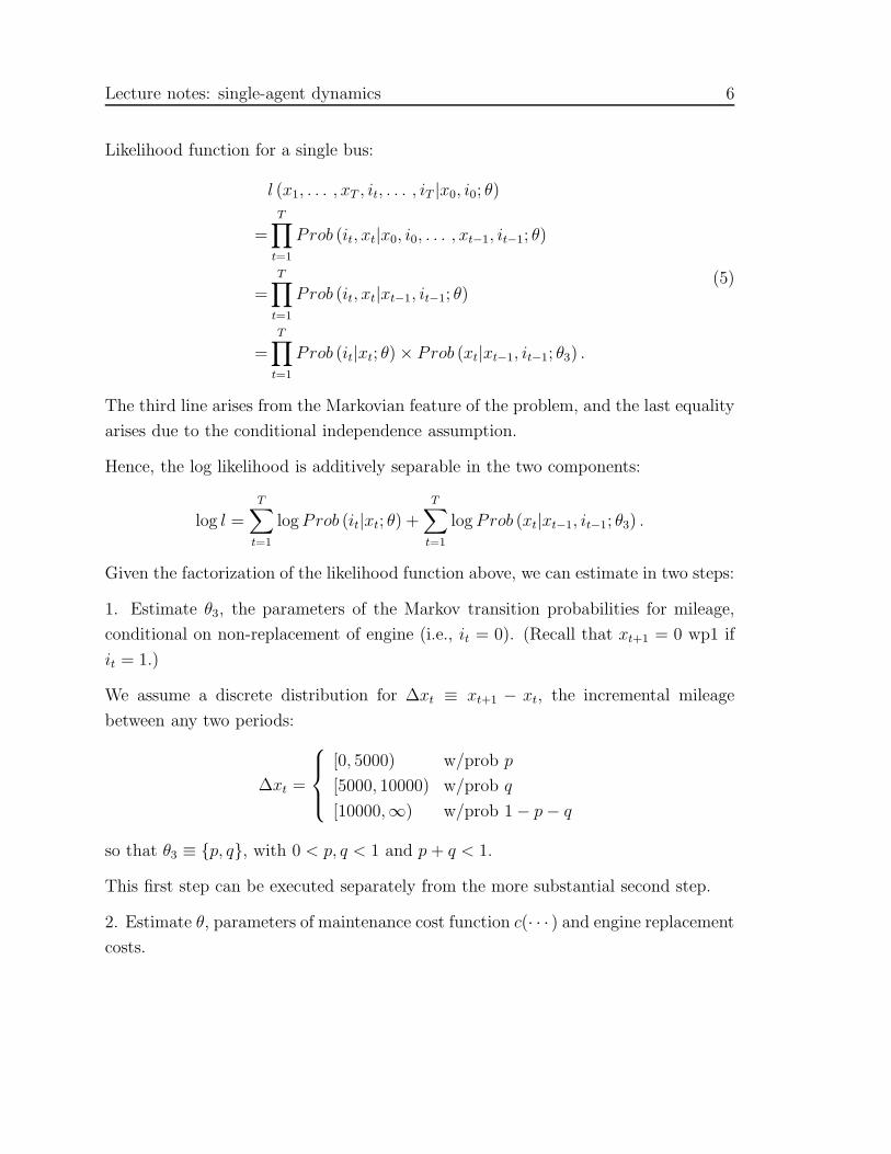
Likelihood function for a single bus:
l (x1, . . . , xT , it, . . . , iT |x0, i0; θ)
=
T∏
t=1
Prob (it, xt|x0, i0, . . . , xt−1, it−1; θ)
=T∏
t=1
Prob (it, xt|xt−1, it−1; θ)
=
T∏
t=1
Prob (it|xt; θ) × Prob (xt|xt−1, it−1; θ3) .
(5)
The third line arises from the Markovian feature of the problem, and the last equality
arises due to the conditional independence assumption.
Hence, the log likelihood is additively separable in the two components:
log l =
T∑
t=1
log Prob (it|xt; θ) +
T∑
t=1
log Prob (xt|xt−1, it−1; θ3) .
Given the factorization of the likelihood function above, we can estimate in two steps:
1. Estimate θ3, the parameters of the Markov transition probabilities for mileage,
conditional on non-replacement of engine (i.e., it = 0). (Recall that xt+1 = 0 wp1 if
it = 1.)
We assume a discrete distribution for ∆xt ≡ xt+1 − xt, the incremental mileage
between any two periods:
∆xt =
[0, 5000) w/prob p
[5000, 10000) w/prob q
[10000,∞) w/prob 1 − p − q
so that θ3 ≡ {p, q}, with 0 < p, q < 1 and p + q < 1.
This first step can be executed separately from the more substantial second step.
2. Estimate θ, parameters of maintenance cost function c(· · · ) and engine replacement
costs.

Lecture notes: single-agent dynamics 7
Here, we make a further assumption that the ǫ’s are distributed i.i.d. (across choices
and periods), according to the Type I extreme value distribution. So this implies that
in Eq. (4) above, p(ǫ′|x′) = p(ǫ′), for all x′.
Expand the expression for Prob(it = 1|xt; θ) equals
Prob{−c(0; θ) − RC + ǫ1t + βEV (0, ǫ′) > −c(xt; θ) + ǫ0t + βEx′,ǫ′|xt,ǫt,it=0V (x′, ǫ′)
}
=Prob{ǫ1t − ǫ0t > c(0; θ) − c(xt; θ) + β
[Ex′,ǫ′|xt,ǫt,it=0V (x, ǫ) − EV (0, ǫ′)
]+ RC
}
Because of the logit assumptions on ǫt, the replacement probability simplifies to a
multinomial logit-like expression:
=exp (−c(0; θ) − RC + βEV (0, ǫ′))
exp (−c(0; θ) − RC + βEV (0, ǫ′)) + exp(−c(xt; θ) + βEx′,ǫ′|xt,ǫt,it=0V (x′, ǫ′)
) .
This is called a “dynamic logit” model, in the literature.
Using the choice-specific utility flow notation, the choice probability takes the form
Prob (it|xt; θ) =exp
(u(xt, it, θ) + βEx′,ǫ′|xt,ǫt,itV (x′, ǫ′)
)
∑
i=0,1 exp(u(xt, i, θ) + βEx′,ǫ′|xt,ǫt,iV (x′, ǫ′)
) . (6)
1.2.1 Estimation method for second step: Nested fixed-point algorithm
The second-step of the estimation procedures is via a “nested fixed point algorithm”.
Outer loop: search over different parameter values θ.
Inner loop: For θ, we need to compute the value function V (x; θ). After V (x, ǫ; θ)
is obtained, we can compute the LL fxn in Eq. (6).
1.2.2 Computational details for inner loop
Compute value function V (x; θ) by iterating over Bellman’s equation (3).
A clever and computationally convenient feature in Rust’s paper is that he iterates
over the expected value function EV (x, i) ≡ Ex′,ǫ′|x,iV (x′, ǫ′; θ). The reason for this is
that you avoid having to calculate the value function at values of ǫ0 and ǫ1, which are
additional state variables. He iterates over the following equation (which is Eq. 4.14
Lecture notes: single-agent dynamics 8
in his paper):
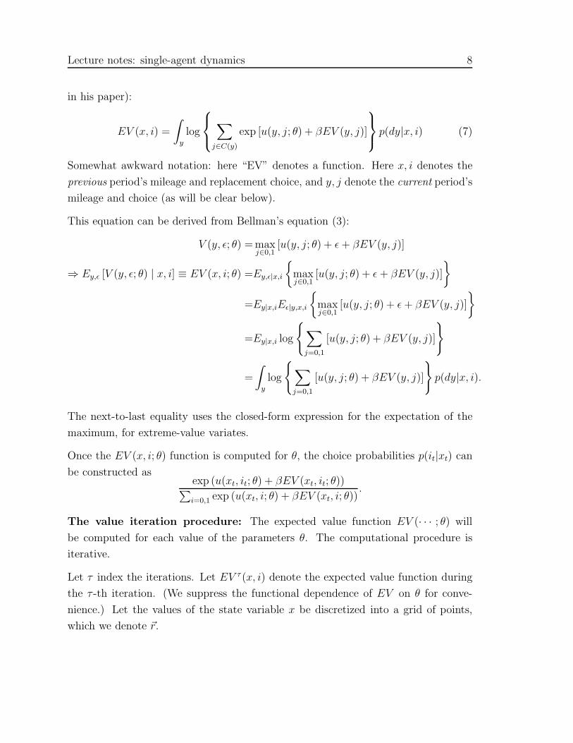
EV (x, i) =
∫
y
log
∑
j∈C(y)
exp [u(y, j; θ) + βEV (y, j)]
p(dy|x, i) (7)
Somewhat awkward notation: here “EV” denotes a function. Here x, i denotes the
previous period’s mileage and replacement choice, and y, j denote the current period’s
mileage and choice (as will be clear below).
This equation can be derived from Bellman’s equation (3):
V (y, ǫ; θ) = maxj∈0,1
[u(y, j; θ) + ǫ + βEV (y, j)]
⇒ Ey,ǫ [V (y, ǫ; θ) | x, i] ≡ EV (x, i; θ) =Ey,ǫ|x,i
{
maxj∈0,1
[u(y, j; θ) + ǫ + βEV (y, j)]
}
=Ey|x,iEǫ|y,x,i
{
maxj∈0,1
[u(y, j; θ) + ǫ + βEV (y, j)]
}
=Ey|x,i log
{∑
j=0,1
[u(y, j; θ) + βEV (y, j)]
}
=
∫
y
log
{∑
j=0,1
[u(y, j; θ) + βEV (y, j)]
}
p(dy|x, i).
The next-to-last equality uses the closed-form expression for the expectation of the
maximum, for extreme-value variates.
Once the EV (x, i; θ) function is computed for θ, the choice probabilities p(it|xt) can
be constructed asexp (u(xt, it; θ) + βEV (xt, it; θ))
∑
i=0,1 exp (u(xt, i; θ) + βEV (xt, i; θ)).
The value iteration procedure: The expected value function EV (· · · ; θ) will
be computed for each value of the parameters θ. The computational procedure is
iterative.
Let τ index the iterations. Let EV τ (x, i) denote the expected value function during
the τ -th iteration. (We suppress the functional dependence of EV on θ for conve-
nience.) Let the values of the state variable x be discretized into a grid of points,
which we denote ~r.

Lecture notes: single-agent dynamics 9
• τ = 0: Start from an initial guess of the expected value function EV (x, i).
Common way is to start with EV (x, i) = 0, for all x ∈ ~r, and i = 0, 1.
• τ = 1: Use Eq. (7) and EV 0(x; θ) to calculate, at each x ∈ ~r, and i ∈ {0, 1}.
EV 1(x, i) =
∫
y
log
∑
j∈C(y)
exp[u(y, j; θ) + βEV 0(y, j)
]
p(dy|x, i)
=p ·
∫ x+5000
x
log
∑
j∈C(y)
exp[u(y, j; θ) + βEV 0(y, j)
]
dy +
q ·
∫ x+10000
x+5000
log {· · · } dy + (1 − p − q) ·
∫ ∞
x+10000
log {· · · } dy.
Now check: is EV 1(x, i) close to EV 0(x, i)? One way is to check whether
supx,i|EV 1(x, i) − EV 0(x, i)| < η
where η is some very small number (eg. 0.0001). If so, then you are done. If
not, then
– Interpolate to get EV 1(·, i) at all points x 6∈ ~r.
– Go to next iteration τ = 2.
2 Hotz-Miller approach: avoid numeric dynamic program-
ming
• One problem with Rust approach to estimating dynamic discrete-choice model
very computer intensive. Requires using numeric dynamic programming to
compute the value function(s) for every parameter vector θ.
• Alternative method of estimation, which avoids explicit DP. Present main ideas
and motivation using a simplified version of Hotz and Miller (1993), Hotz, Miller,
Sanders, and Smith (1994).
• For simplicity, think about Harold Zurcher model.

Lecture notes: single-agent dynamics 10
• What do we observe in data from DDC framework? For bus i, time t, observe:
– {xit, dit}: observed state variables xit and discrete decision (control) vari-
able dit. For simplicity, assume dit is binary, ∈ {0, 1}
Let i = 1, . . . , N index the buses, t = 1, . . . , T index the time periods.
– For Harold Zurcher model: xit is mileage on bus i in period t, and dit is
whether or not engine of bus i was replaced in period t.
– Given renewal assumptions (that engine, once repaired, is good as new),
define transformed state variable xit: mileage since last engine change.
– Unobserved state variables: ǫit, i.i.d. over i and t. Assume that distribution
is known (Type 1 Extreme Value in Rust model)
• In the following, let quantities with hats ’s denote objects obtained just from
data.
Objects with tildes ’s denote “predicted” quantities, obtained from both data
and calculated from model given parameter values θ.
• From this data alone, we can estimate (or “identify”):
– Transition probabilities of observed state and control variables: G(x′|x, d)1,
estimated by conditional empirical distribution
G(x′|x, d) ≡
{ ∑N
i=1
∑T−1t=1
1P
i
P
t1(xit=x,dit=0)
· 1 (xi,t+1 ≤ x′, xit = x, dit = 0) , if d = 0∑N
i=1
∑T−1t=1
1P
i
P
t1(dit=1)
· 1 (xi,t+1 ≤ x′, dit = 1) , if d = 1.
– Choice probabilities, conditional on state variable: Prob (d = 1|x)2, esti-
mated by
P (d = 1|x) ≡
N∑
i=1
T−1∑
t=1
1∑
i
∑
t 1 (xit = x)· 1 (dit = 1, xit = x) .
Since Prob (d = 0|x) = 1−Prob (d = 1|x), we have P (d = 0|x) = 1−P (d =
1|x).
1By stationarity, note we do not index the G function explicitly with time t.2By stationarity, note we do not index this probability explicitly with time t.
Lecture notes: single-agent dynamics 11
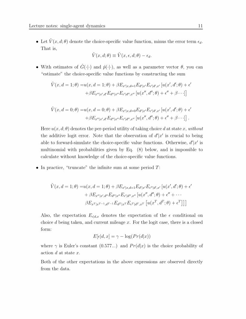
• Let V (x, d; θ) denote the choice-specific value function, minus the error term ǫd.
That is,
V (x, d; θ) ≡ V (x, ǫ, d; θ) − ǫd.
• With estimates of G(·|·) and p(·|·), as well as a parameter vector θ, you can
“estimate” the choice-specific value functions by constructing the sum
V (x, d = 1; θ) =u(x, d = 1; θ) + βEx′|x,d=1Ed′|x′Eǫ′|d′,x′ [u(x′, d′; θ) + ǫ′
+βEx′′|x′,d′Ed′′|x′′Eǫ′|d′′,x′′ [u(x′′, d′′; θ) + ǫ′′ + β · · ·]]
V (x, d = 0; θ) =u(x, d = 0; θ) + βEx′|x,d=0Ed′|x′Eǫ′|d′,x′ [u(x′, d′; θ) + ǫ′
+βEx′′|x′,d′Ed′′|x′′Eǫ′|d′′,x′′ [u(x′′, d′′; θ) + ǫ′′ + β · · ·]].
Here u(x, d; θ) denotes the per-period utility of taking choice d at state x, without
the additive logit error. Note that the observation of d′|x′ is crucial to being
able to forward-simulate the choice-specific value functions. Otherwise, d′|x′ is
multinomial with probabilities given by Eq. (8) below, and is impossible to
calculate without knowledge of the choice-specific value functions.
• In practice, “truncate” the infinite sum at some period T :
V (x, d = 1; θ) =u(x, d = 1; θ) + βEx′|x,d=1Ed′|x′Eǫ′′|d′,x′ [u(x′, d′; θ) + ǫ′
+ βEx′′|x′,d′′Ed′′|x′′Eǫ′|d′′,x′′ [u(x′′, d′′; θ) + ǫ′′ + · · ·
βExT |xT−1,dT−1EdT |xT EǫT |dT ,xT
[u(xT , dT ; θ) + ǫT
]]]
Also, the expectation Eǫ|d,x denotes the expectation of the ǫ conditional on
choice d being taken, and current mileage x. For the logit case, there is a closed
form:
E[ǫ|d, x] = γ − log(Pr(d|x))
where γ is Euler’s constant (0.577...) and Pr(d|x) is the choice probability of
action d at state x.
Both of the other expectations in the above expressions are observed directly
from the data.

Lecture notes: single-agent dynamics 12
• Both choice-specific value functions can be simulated by (for d = 1, 2):
V (x, d; θ) ≈ =1
S
∑
s
[
u(x, d; θ) + β[
u(x′s, d′s; θ) + γ − log(P (d′s|x′s))
+β[
u(x′′s, d′′s; θ) + γ − log(P (d′′s|x′′s)) + β · · ·]]]
where
– x′s ∼ G(·|x, d)
– d′s ∼ p(·|x′s), x′′s ∼ G(·|x′s, d′s)
– &etc.
In short, you simulate V (x, d; θ) by drawing S “sequences” of (dt, xt) with a
initial value of (d, x), and computing the present-discounted utility correspond
to each sequence. Then the simulation estimate of V (x, d; θ) is obtained as the
sample average.
• Given an estimate of V (·, d; θ), you can get the predicted choice probabilities:
p(d = 1|x; θ) ≡exp
(
V (x, d = 1; θ))
exp(
V (x, d = 1; θ))
+ exp(
V (x, d = 0; θ)) (8)
and analogously for p(d = 0|x; θ). Note that the predicted choice probabilities
are different from p(d|x), which are the actual choice probabilities computed
from the actual data. The predicted choice probabilities depend on the param-
eters θ, whereas p(d|x) depend solely on the data.
• One way to estimate θ is to minimize the distance between the predicted con-
ditional choice probabilities, and the actual conditional choice probabilities:
θ = argminθ||p(d = 1|x) − p (d = 1|x; θ) ||
where p denotes a vector of probabilities, at various values of x.
• Another way to estimate θ is very similar to the Berry/BLP method. We can
calculate directly from the data.
δx ≡ log p(d = 1|x) − log p(d = 0|x)

Lecture notes: single-agent dynamics 13
Given the logit assumption, from equation (8), we know that
log p(d = 1|x) − log p(d = 0|x) =[
V (x, d = 1) − V (x, d = 0)]
.
Hence, by equating V (x, d = 1) − V (x, d = 0) to δx, we obtain an alternative
estimator for θ:
θ = argminθ||δx −[
V (x, d = 1; θ) − V (x, d = 0; θ)]
||.
2.1 A useful representation for the discrete state case
For the case when the state variables S are discrete, the value function is just a
vector, and it turns out that, given knowledge of the CCP’s P (Y |S), solving the
value function is just equivalent to solving a system of linear equations. This was
pointed out in Pesendorfer and Schmidt-Dengler (2007) and Aguirregabiria and Mira
(2007), and we follow the treatment in the latter paper. Specifically:
• Assume that choices Y and state variables S are all discrete. |S| is cardinality
of state space S.
• Per-period utilities:
u(Y, S, ǫY ) = u(Y, S) + ǫY
where ǫY , for y = 1, . . . Y , are i.i.d. extreme value distributed with unit variance.
• Parameters Θ. The discount rate β is treated as known and fixed.
V (S; Θ), which is the vector (each element denotes a different value of S) for
the value function at the parameter Θ, is given by
V (S; Θ) = (I − βF )−1
∑
Y ∈(0,1)
P (Y ) ∗ [u(Y ) + ǫ(Y )]
(9)
where
– ’*’ denotes elementwise multiplication

Lecture notes: single-agent dynamics 14
– F is the |S|-dimensional square matrix with (i, j)-element equal to
Pr(S ′ = j|S = i) ≡∑
Y =(0,1)
P (Y |S = i) · Pr(S ′ = j|S = i, Y ). (10)
– P (Y ) is the |S|-vector consisting of elements Pr(Y |S).
– u(Y ) is the |S|-vector of per-period utilities u(Y ; S).
– ǫ(Y ) is an |S|-vector where each element is E[ǫY |Y , S]. For the logit as-
sumptions, the closed-form is
E[ǫY |Y , S] = Euler’s constant − log(P (Y |S)).
Euler’s constant is 0.57721.
2.2 Semiparametric identification of DDC Models
We can also use the Hotz-Miller estimation scheme as a basis for an argument re-
garding the identification of the underlying DDC model. In Markovian DDC models,
without unobserved state variables, the Hotz-Miller routine exploits the fact that the
Markov probabilities x′, d′|x, d are identiified directly from the data, which can be
factorized into
f(x′, d′|x, d) = f(d′|x′)︸ ︷︷ ︸
CCP
· f(x′|x, d)︸ ︷︷ ︸
state law of motion
.(11)
In this section, we argue that once these “reduced form” components of the model
are identified, the remaining parts of the models – particularly, the per-period utility
functions – can be identified without any further parametric assumptions. These
arguments are drawn from Magnac and Thesmar (2002) and Bajari, Chernozhukov,
Hong, and Nekipelov (2007).
We make the following assumptions, which are standard in this literature:
1. Agents are optimizing in an infinite-horizon, stationary setting. Therefore, in
the rest of this section, we use primes ′’s to denote next-period values.
2. Actions D are chosen from the set D = {0, 1, . . . , K}.

Lecture notes: single-agent dynamics 15
3. The state variables are X.
4. The per-period utility from taking action d ∈ D in period t is:
ud(Xt) + ǫd,t, ∀d ∈ D.
The ǫd,t’s are utility shocks which are independent of Xt, and distributed i.i.d
with known distribution F (ǫ) across periods t and actions d. Let ~ǫt ≡ (ǫ0,1, ǫ1,t, . . . , ǫK,t).
5. From the data, the “conditional choice probabilities” CCP’s
pd(X) ≡ Prob(D = 1|X),
and the Markov transition kernel for X, denoted p(X ′|D, X), are identified.
6. u0(S), the per-period utility from D = 0, is normalized to zero, for all X.
7. β, the discount factor, is known.3
Following the arguments in Magnac and Thesmar (2002) and Bajari, Chernozhukov,
Hong, and Nekipelov (2007), we will show the nonparametric identification of ud(·), d =
1, . . . , K, the per-period utility functions for all actions except D = 0.
The Bellman equation for this dynamic optimization problem is
V (X,~ǫ) = maxd∈D
(ud(X) + ǫd + βEX′,~ǫ′|D,XV (X ′,~ǫ′)
)
where V (X,~ǫ) denotes the value function. We define the choice-specific value function
as
Vd(X) ≡ ud(X) + βEX′,~ǫ′|D,XV (X ′,~ǫ′).
Given these definitions, an agent’s optimal choice when the state is X is given by
y∗(X) = argmaxy∈D (Vd(X) + ǫd) .
3Magnac and Thesmar (2002) discuss the possibility of identifying β via exclusion restrictions,
but we do not pursue that here.
Lecture notes: single-agent dynamics 16
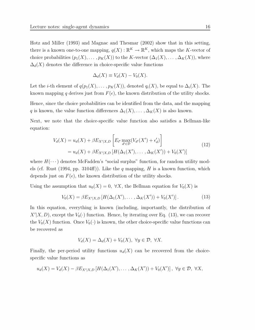
Hotz and Miller (1993) and Magnac and Thesmar (2002) show that in this setting,
there is a known one-to-one mapping, q(X) : RK → R
K , which maps the K-vector of
choice probabilities (p1(X), . . . , pK(X)) to the K-vector (∆1(X), . . . , ∆K(X)), where
∆d(X) denotes the difference in choice-specific value functions
∆d(X) ≡ Vd(X) − V0(X).
Let the i-th element of q(p1(X), . . . , pK(X)), denoted qi(X), be equal to ∆i(X). The
known mapping q derives just from F (ǫ), the known distribution of the utility shocks.
Hence, since the choice probabilities can be identified from the data, and the mapping
q is known, the value function differences ∆1(X), . . . , ∆K(X) is also known.
Next, we note that the choice-specific value function also satisfies a Bellman-like
equation:
Vd(X) = ud(X) + βEX′|X,D
[
E~ǫ′ maxd′∈D
(Vd′(X′) + ǫ′d)
]
= ud(X) + βEX′|X,D [H(∆1(X′), . . . , ∆K(X ′)) + V0(X
′)]
(12)
where H(· · · ) denotes McFadden’s “social surplus” function, for random utility mod-
els (cf. Rust (1994, pp. 3104ff)). Like the q mapping, H is a known function, which
depends just on F (ǫ), the known distribution of the utility shocks.
Using the assumption that u0(X) = 0, ∀X, the Bellman equation for V0(X) is
V0(X) = βEX′|X,D [H(∆1(X′), . . . , ∆K(X ′)) + V0(X
′)] . (13)
In this equation, everything is known (including, importantly, the distribution of
X ′|X, D), except the V0(·) function. Hence, by iterating over Eq. (13), we can recover
the V0(X) function. Once V0(·) is known, the other choice-specific value functions can
be recovered as
Vd(X) = ∆d(X) + V0(X), ∀y ∈ D, ∀X.
Finally, the per-period utility functions ud(X) can be recovered from the choice-
specific value functions as
ud(X) = Vd(X) − βEX′|X,D [H(∆1(X′), . . . , ∆K(X ′)) + V0(X
′)] , ∀y ∈ D, ∀X,

Lecture notes: single-agent dynamics 17
where everything on the right-hand side is known.
Remark: For the case where F (ǫ) is the Type 1 Extreme Value distribution, the
social surplus function is
H(∆1(X), . . . , ∆K(X)) = log
[
1 +
K∑
d=1
exp(∆d(X))
]
and the mapping q is such that
qd(X) = ∆d(X) = log(pd(X)) − log(p0(X)), ∀d = 1, . . .K,
where p0(X) ≡ 1 −∑K
d=1 pd(X). �
3 Model with persistence in unobservables (“unobserved state
variables”)
Up to now, we consider models satisfying Rust’s “conditional independence” assump-
tion on the ǫ’s. This rules out persistence in unobservables, which can be economically
meaningful.
In this section, we consider estimation of a more general model, in which ǫ’s can
be serially correlated over time: now ǫ is a nontrivial unobserved state variables (it
cannot just be integrated out, as in the Eq. (7) above).
For convenience: in this section we use x to denote observed state variable, ǫ to denote
unobserved state variable, and i to denote the control variable.
Now we allow ǫ to evolve as a controlled first-order Markov process, evolving according
to: F (ǫ′|ǫ, x, d).
We continue to assume, as before, that the policy function is i(x, ǫ), and that the state
evolution does not depend explicitly on ǫ: next period’s state evolves as in x′|x, d.
Given these assumption, the analogue of Eq. (4) is:
p(x′, ǫ′|x, ǫ, i) = p(ǫ′|x′, x, ǫ, i) · p(x′|x, ǫ, i)
= p(ǫ′|x′, ǫ, i) · p(x′|x, i).(14)

Lecture notes: single-agent dynamics 18
Now the likelihood function for a single bus:
l (x1, . . . , xT , it, . . . , iT |x0, i0; θ)
=
T∏
t=1
Prob (it, xt|x0, i0, . . . , xt−1, it−1; θ)
=T∏
t=1
Prob (it|xt, x0, i0, . . . , xt−1, it−1; θ) × Prob (xt|xt−1, it−1; θ3) .
(15)
Note that because of the serially correlated ǫ’s, there is still dependence between (say)
it and it−2, even after conditioning on (xt−1, it−1): compare the last lines of Eq. (5)
and Eq. (15).
Now, because of serially correlation in the ǫ’s, the Prob (it|xt, x0, i0, . . . , xt−1, it−1; θ)
no longer has a closed form. Thus, we consider simulating the likelihood function.
Note that simulation is part of the “outer loop” of nested fixed point estimation
routine. So at the point when we simulate, we already know the policy function
i(x, ǫ; θ) and choice-specific value functions V (x, ǫ, i; θ) for each possible choice i.
3.1 “Crude” frequency simulator
Since (x, i, ǫ) all evolve together, we cannot just draw the ǫ process separately from
(i, x). Thus for simulation purposes, it is most convenient to go back to the full
likelihood function (the first line of Eq. (15):
l(x1, . . . , xT , i1, . . . , iT |x0, i0, ǫ0; θ).
Note that because the ǫ’s are serially correlated, we also need to condition on an
initial value ǫ0 (which, for simplicity, we assume ǫ0 = 0, or that it is known).
For the case where (i, x) are both discrete (as in Rust’s paper), the likelihood is the
joint probability
Pr(ǫ1, . . . , ǫT , X1, . . . , XT : Xt = xt, i(Xt, ǫt; θ) = it, ∀t = 1, . . . , T ).
In the above, X1, . . . , XT (capital letters) denotes the mileage random variable, and
x1, . . . , xT (lower case) denotes the observed mileage in the dataset. Let F (ǫ′|x, i, ǫ; γ)

Lecture notes: single-agent dynamics 19
denote the transition density for the ǫ’s, and G(X ′|X, i; θ3) the transition probability
for the X’s. Then the above probability can be expressed as the integral:
∫
· · ·
∫∏
t
1(Xt = xt)1(i(Xt, ǫt; θ) = it)∏
t
dF (ǫt|ǫt−1, Xt−1, i(Xt−1, ǫt−1; γ))dG(Xt|Xt−1, i(Xt−1, ǫt); θ3).
We can simulate this integral by drawing sequences of (Xt, ǫt). For each simulation
draw s = 1, . . . , S, we take as initial values x0, i0, ǫ0. Then:
• Generate (ǫs1, x
s1, i
s1):
1. Generate ǫs1 ∼ F (ǫ|x0, i0, ǫ0)
2. Generate xs1 ∼ G(x|x0, i0)
3. Subsequently compute is1 = i(xs1, ǫ
s1; θ)
• Generate (ǫs2, x
s2, i
s2):
1. Generate ǫs2 ∼ F (ǫ|xs
1, is1, ǫ
s1)
2. Generate xs2 ∼ G(x|xs
1, is1)
3. Subsequently compute is2 = i(xs2, ǫ
s2; θ)
... and so on, up to (ǫsT , xs
T , isT )
Then, for the case where (i, x) are both discrete (which is the case in Rust’s paper),
we can approximate
l (x1, . . . , xT , it, . . . , iT |x0, i0; θ) ≈1
S
∑
s
T∏
t=1
1(xst = xt) · 1(ist = it).
That is, the simulated likelihood is the frequency of the simulated sequences which
match the observed sequence.
Gory details This is a “crude” frequency simulator. Clearly, if T is long, or S
is modest, the simulated likelihood is likely to be zero. What is commonly done in
practice is to smooth the indicator functions in this simulated likelihood.
Lecture notes: single-agent dynamics 20
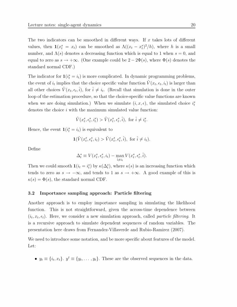
The two indicators can be smoothed in different ways. If x takes lots of different
values, then 1(xst = xt) can be smoothed as Λ((xt − xs
t )2/h), where h is a small
number, and Λ(s) denotes a decreasing function which is equal to 1 when s = 0, and
equal to zero as s → +∞. (One example could be 2− 2Φ(s), where Φ(s) denotes the
standard normal CDF.)
The indicator for 1(ist = it) is more complicated. In dynamic programming problems,
the event of it implies that the choice specific value function V (xt, ǫt, it) is larger than
all other choices V (xt, ǫt, i), for i 6= it. (Recall that simulation is done in the outer
loop of the estimation procedure, so that the choice-specific value functions are known
when we are doing simulation.) When we simulate (i, x, ǫ), the simulated choice istdenotes the choice i with the maximum simulated value function:
V (xst , ǫ
st , i
st) > V (xs
t , ǫst , i), for i 6= ist .
Hence, the event 1(ist = it) is equivalent to
1(V (xst , ǫ
st , it) > V (xs
t , ǫst , i), for i 6= it).
Define
∆st ≡ V (xs
t , ǫst , it) − max
i6=it
V (xst , ǫ
st , i).
Then we could smooth 1(it = ist ) by κ(∆st ), where κ(s) is an increasing function which
tends to zero as s → −∞, and tends to 1 as s → +∞. A good example of this is
κ(s) = Φ(s), the standard normal CDF.
3.2 Importance sampling approach: Particle filtering
Another approach is to employ importance sampling in simulating the likelihood
function. This is not straightforward, given the across-time dependence between
(it, xt, ǫt). Here, we consider a new simulation approach, called particle filtering. It
is a recursive approach to simulate dependent sequences of random variables. The
presentation here draws from Fernandez-Villaverde and Rubio-Ramirez (2007).
We need to introduce some notation, and be more specific about features of the model.
Let:
• yt ≡ {it, xt}. yt ≡ {yt, . . . , yt}. These are the observed sequences in the data.

Lecture notes: single-agent dynamics 21
• Evolution of utility shocks: ǫt|ǫt−1 ∼ f(ǫ′|ǫ). Eliminate dependence of ǫt on xt,
it.
• Evolution of mileage: xt = h(xt−1, it−1, wt). Mileage xt evolves deterministically,
according to the h function. wt is a new “mileage shock”, which is assumed to
be distributed iid over time, according to density g(w). An example of h(· · · )
is
xt =
{
xt−1 + wt if it−1 = 0
wt otherwise.
Assume h(· · · ) is invertible in third argument, and define φ(xt−1, it−1, xt) as this
inverse function, satisfying
xt = h(xt−1, it−1, φ(xt−1, it−1, xt)).
• As before, the policy function is it = i(xt, ǫt).
• Let ǫt ≡ {ǫ1, . . . , ǫt}.
• The initial values y0 and ǫ0 are known.
Go back to the factorized likelihood:
l(yT |y0, ǫ) =
T∏
t=1
l(yt|yt−1, y0, ǫ0)
=∏
t
∫
l(yt|ǫt, yt−1)p(ǫt|yt−1)dǫt
≈∏
t
1
S
∑
s
l(yt|ǫt|t−1,s, yt−1)
(16)
where in the second to last line, we omit conditioning on (y0, ǫ0) for convenience. In
the last line, ǫt|t−1,s denotes simulated draws of ǫt from p(ǫt|yt−1).
Consider the two terms in the last line:

Lecture notes: single-agent dynamics 22
• The first term:
l(yt|ǫt, yt−1) = p(it, xt|ǫ
t, yt−1)
= p(it|xt, ǫt, yt−1) · p(xt|ǫ
t, yt−1)
= p(it|xt, ǫt) · p(xt|it−1, xt−1)
= 1(i(xt, ǫt) = it) · g(φ(xt−1, it−1, xt)) ·∂h
∂w
∣∣w=φ(xt−1,it−1,xt)
(17)
where the last two terms in the last line is the Jacobian of the transformation
from w to x. This term can be explicitly calculated, for a given value of ǫt.
• The second term is, generally, not obtainable in closed form. So numerical
integration not feasible. The particle filtering algorithm permits us to draw
sequences of ǫt from p(ǫt|yt−1), for every period t. Hence, the last line of (16)
can be approximated by simulation.
Particle filtering proposes a recursive approach to draw sequences from p(ǫt|yt−1), for
every t. Easiest way to proceed is just to describe the algorithm.
First period, t = 1: In order to simulate the integral corresponding to the first
period, we need to draw from p(ǫ1|y0, ǫ0). This is easy. We draw{ǫ1|0,s
}S
s=1, according
to f(ǫ′|ǫ0). The notation ǫ1|0,s makes explicitly that the ǫ is a draw from p(ǫ1|y0, ǫ0).
Using these S draws, we can evaluate the simulated likelihood for period 1, in Eq.
(16). We are done for period t = 1.
Second period, t = 2: We need to draw from p(ǫ2|y1). Factorize this as:
p(ǫ2|y1) = p(ǫ1|y1) · p(ǫ2|ǫ1). (18)
Recall our notation that ǫ2 ≡ {ǫ1, ǫ2}. Consider simulating from each term separately:
• Getting a draw from p(ǫ1|y1), given that we already have draws{ǫ1|0,s
}from
p(ǫ1|y0), from the previous period t = 1, is the heart of particle filtering.
We use the principle of importance sampling: by Bayes’ Rule,
p(ǫ1|y1) ∝ p(y1|ǫ1, y0) · p(ǫ1|y0)
Lecture notes: single-agent dynamics 23
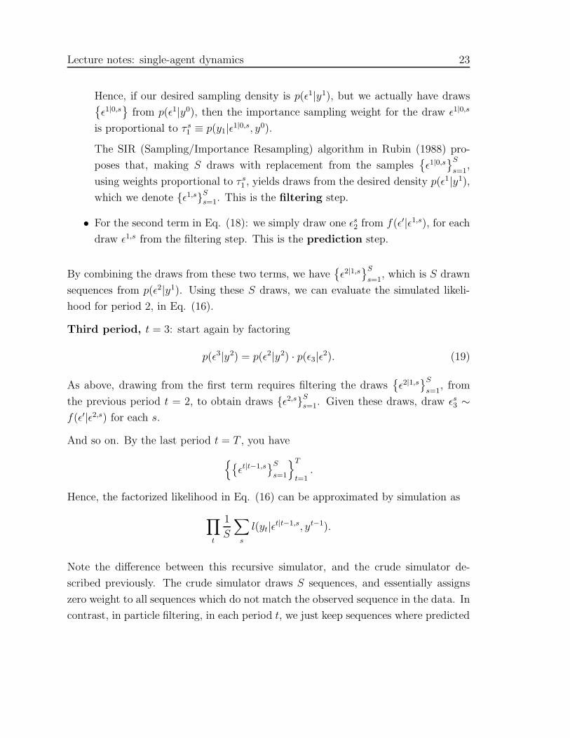
Hence, if our desired sampling density is p(ǫ1|y1), but we actually have draws{ǫ1|0,s
}from p(ǫ1|y0), then the importance sampling weight for the draw ǫ1|0,s
is proportional to τ s1 ≡ p(y1|ǫ
1|0,s, y0).
The SIR (Sampling/Importance Resampling) algorithm in Rubin (1988) pro-
poses that, making S draws with replacement from the samples{ǫ1|0,s
}S
s=1,
using weights proportional to τ s1 , yields draws from the desired density p(ǫ1|y1),
which we denote {ǫ1,s}S
s=1. This is the filtering step.
• For the second term in Eq. (18): we simply draw one ǫs2 from f(ǫ′|ǫ1,s), for each
draw ǫ1,s from the filtering step. This is the prediction step.
By combining the draws from these two terms, we have{ǫ2|1,s
}S
s=1, which is S drawn
sequences from p(ǫ2|y1). Using these S draws, we can evaluate the simulated likeli-
hood for period 2, in Eq. (16).
Third period, t = 3: start again by factoring
p(ǫ3|y2) = p(ǫ2|y2) · p(ǫ3|ǫ2). (19)
As above, drawing from the first term requires filtering the draws{ǫ2|1,s
}S
s=1, from
the previous period t = 2, to obtain draws {ǫ2,s}S
s=1. Given these draws, draw ǫs3 ∼
f(ǫ′|ǫ2,s) for each s.
And so on. By the last period t = T , you have
{{ǫt|t−1,s
}S
s=1
}T
t=1.
Hence, the factorized likelihood in Eq. (16) can be approximated by simulation as
∏
t
1
S
∑
s
l(yt|ǫt|t−1,s, yt−1).
Note the difference between this recursive simulator, and the crude simulator de-
scribed previously. The crude simulator draws S sequences, and essentially assigns
zero weight to all sequences which do not match the observed sequence in the data. In
contrast, in particle filtering, in each period t, we just keep sequences where predicted

Lecture notes: single-agent dynamics 24
choices match observed choice that period. This will lead to more accurate evalua-
tion of the likelihood. Note that S should be large enough (relative to the sequence
length T ) so that the filtering step does not end up assigning almost all weight to one
particular sequence ǫt|t−1,s in any period t.

Lecture notes: single-agent dynamics 25
References
Aguirregabiria, V., and P. Mira (2007): “Sequential Estimation of Dynamic DiscreteGames,” Econometrica, 75, 1–53.
Bajari, P., V. Chernozhukov, H. Hong, and D. Nekipelov (2007): “Nonparametricand Semiparametric Analysis of a Dynamic Game Model,” Manuscript, University ofMinnesota.
Chevalier, J., and A. Goolsbee (2005): “Are Durable Goods Consumers ForwardLooking?,” NBER working paper 11421.
Fernandez-Villaverde, J., and J. Rubio-Ramirez (2007): “Estimating Macroeco-nomic Models: A Likelihood Approach,” University of Pennsylvania, working paper.
Hotz, J., and R. Miller (1993): “Conditional Choice Probabilties and the Estimationof Dynamic Models,” Review of Economic Studies, 60, 497–529.
Hotz, J., R. Miller, S. Sanders, and J. Smith (1994): “A Simulation Estimator forDynamic Models of Discrete Choice,” Review of Economic Studies, 61, 265–289.
Magnac, T., and D. Thesmar (2002): “Identifying Dynamic Discrete Decision Pro-cesses,” Econometrica, 70, 801–816.
Pesendorfer, M., and P. Schmidt-Dengler (2007): “Asymptotic Least Squares Esti-mators for Dynamic Games,” Review of Economic Studies, forthcoming.
Rubin, D. (1988): “Using the SIR Algorithm to Simulate Posterior Distributions,” inBayesian Statistics 3, ed. by J. Bernardo, M. DeGroot, D. Lindley, and A. Smith. OxfordUniversity Press.
Rust, J. (1987): “Optimal Replacement of GMC Bus Engines: An Empirical Model ofHarold Zurcher,” Econometrica, 55, 999–1033.
(1994): “Structural Estimation of Markov Decision Processes,” in Handbook of
Econometrics, Vol. 4, ed. by R. Engle, and D. McFadden, pp. 3082–146. North Holland.