singular spdes and related topics - tu berlin · singular spdes and related topics vorgelgt von...
TRANSCRIPT
Singular SPDEs and Related Topics
VORGELGT VON
GIUSEPPE CANNIZZAROgeb. in Padova
VON DER FAKULTAT II - MATHEMATIK UND NATURWISSENSCHAFTENDER TECHNISCHEN UNIVERSITAT BERLIN
ZUR ERLANGUNG DES AKADEMISCHEN GRADES
DOKTOR DER NATURWISSENSCHAFTENDR. RER. NAT.
genehmigte Dissertation
Promotionausschuss
Vorsitzender: PROF. DR. BORIS SPRINGBORN
Berichter/Gutachter: PROF. DR. PETER K. FRIZBerichter/Gutachter: PROF. DR. FRANCOIS DELARUE
Tag der wissenschaftlichen Aussprache: 15. September 2016
Berlin 2016


to Panci

Acknowledgements
The first person I want to thank is my advisor Prof. Peter K. Friz. He has always been available for discussions onmy work, wisely directing my research, and sensibly nurtured my interest for the topics developed in this thesis. Hisclarity of thoughts, fruitful advices, both mathematically and academically, and his own passion have been a trulysource of stimulus and inspiration to me.
A special thank goes to Khalil Chouk, among the various, for the research we have done toghether and thefriendship he has shown me throughout these years. Hoping we will keep on collaborating in the future, please stoptrying to spoil GoT. I will watch it. Promised.
I would also like to sincerely express my gratitude to all the other people with whom I had the pleasure tocollaborate and share the pain and the happyness that mathematics naturally entails, Paul Gassiat, KonstantinMatetski, Prof. Dirk Blomker and Prof. Marco Romito. I want to thank Prof. M. Hairer and Prof. M. Gubinelli formany fruitful discussions and the possibility to spend some time in Warwick and Paris. I would also like to expressmy gratitude to all the professors that I could visit during my years of PhD, starting from my master thesis advisorProf. P. Dai Pra, but also Prof. D. Blomker and Prof. M. Romito, and, more generally, to all professors (and aspecial mention goes to Prof. N. Perkowski), researchers and postdocs, from my advisor’s group and not, that haveso generously shared their knowledge and time with me, contributing to my personal and academical growth.
I also want to thank to Prof. Francois Delarue for accepting to be the external reviewer of this thesis.
Sharing the office with Matti, Benedikt and Massimo was simply great. I want to thank Matti for introducing meto Germany and the germans, teaching me (or bearing my attempts to speak) german and exploring with me Berlinwhile Massimo for being the friend of a lifetime, with whom I basically grew up, both mathematically and phisically.They and the guys of the office in front (Adrian, Alberto, Atul, Giovanni and Sara) were my first approach to thiscity and are the ones that made my experience here unique, ca va sans dir, they all deserve a huge thank you. (Ithink at this point I might even call you “friends”...)
I want to thank all the people in the RTG and at TU Berlin with whom I spent and enjoyed these years, Elena andFilippo for the restoring italian dinners and my flatemates (and of course their partners) who endured my volatilepresence and my excessive verboseness.
I want to particularly thank my parents and sister, as well as my whole family, for believing in me and supportingme in all possible situations and with all possible means. I am sincerely thankful to all the long-distance help thatcame from my italian friends, the time they spent on skype (and in person) with me and their trips to Berlin.
The last and most important person I want to express my deepest gratitude to is without any doubts my girlfriend,Panci. She stood by my side all these years no matter what, giving me the right perspective when I lost it and thestrongest support when I needed it. If I managed to go through my PhD I owe it to you and to you I dedicate thisthesis.
I acknowledge financial support from the DFG Research Training Group 1845 (scholarship) and support fortravelling from the Berlin Mathematical School (BMS).
i

ii
Contents
Summary vi
Zusammenfassung vii
1 Introduction 11.1 SDEs with Distributional Drift . . . . . . . . . . . . . . . . . . . . . . . . . . . . . . . . . . . . 21.2 The Polymer Measure with White Noise Potential . . . . . . . . . . . . . . . . . . . . . . . . . . 41.3 Malliavin Calculus and Regularity Structures . . . . . . . . . . . . . . . . . . . . . . . . . . . . 5
2 Multidimensional SDEs with Distributional Drift and Polymer Measure 92.0.1 Function Spaces and Notations . . . . . . . . . . . . . . . . . . . . . . . . . . . . . . . . 10
2.1 Description of the main results . . . . . . . . . . . . . . . . . . . . . . . . . . . . . . . . . . . . 112.2 Well-posedness of the martingale problem . . . . . . . . . . . . . . . . . . . . . . . . . . . . . . 132.3 Operations with Besov-Holder functions . . . . . . . . . . . . . . . . . . . . . . . . . . . . . . . 152.4 Solving the Generator equation . . . . . . . . . . . . . . . . . . . . . . . . . . . . . . . . . . . . 17
2.4.1 The Young case: β ∈ (− 12 , 0) . . . . . . . . . . . . . . . . . . . . . . . . . . . . . . . . 18
2.4.2 The rough case: β ∈− 2
3 ,−12
. . . . . . . . . . . . . . . . . . . . . . . . . . . . . . . 19
2.5 Construction of the Polymer Measure . . . . . . . . . . . . . . . . . . . . . . . . . . . . . . . . 242.6 A KPZ-type equation driven by a purely spatial white noise . . . . . . . . . . . . . . . . . . . . . 26
2.6.1 Analytic part . . . . . . . . . . . . . . . . . . . . . . . . . . . . . . . . . . . . . . . . . 272.6.2 Stochastic part . . . . . . . . . . . . . . . . . . . . . . . . . . . . . . . . . . . . . . . . 332.6.3 The Renormalization Constants . . . . . . . . . . . . . . . . . . . . . . . . . . . . . . . 42
2.7 The Polymer Measure and its properties . . . . . . . . . . . . . . . . . . . . . . . . . . . . . . . 472.7.1 Proof of the Proposition 2.5.1 . . . . . . . . . . . . . . . . . . . . . . . . . . . . . . . . 472.7.2 Global existence, Parabolic Anderson equation and Feynman-Kac representation . . . . . 482.7.3 Singularity with respect to the Wiener measure . . . . . . . . . . . . . . . . . . . . . . . 48
3 Malliavin Calculus for Regularity Structures: the case of gPAM 513.1 Malliavin Calculus in a nutshell . . . . . . . . . . . . . . . . . . . . . . . . . . . . . . . . . . . 523.2 The framework . . . . . . . . . . . . . . . . . . . . . . . . . . . . . . . . . . . . . . . . . . . . 53
3.2.1 The Regularity Structure for gPAM . . . . . . . . . . . . . . . . . . . . . . . . . . . . . 533.2.2 Enlarging Tg . . . . . . . . . . . . . . . . . . . . . . . . . . . . . . . . . . . . . . . . . 553.2.3 Admissible Models . . . . . . . . . . . . . . . . . . . . . . . . . . . . . . . . . . . . . . 563.2.4 Extension and Translation of Admissible Models . . . . . . . . . . . . . . . . . . . . . . 583.2.5 Extending the Renormalization Group . . . . . . . . . . . . . . . . . . . . . . . . . . . . 623.2.6 Convergence of the Renormalized Models . . . . . . . . . . . . . . . . . . . . . . . . . . 643.2.7 Modelled Distributions and Fixed Point argument . . . . . . . . . . . . . . . . . . . . . . 653.2.8 Weak maximum principles and gPAM . . . . . . . . . . . . . . . . . . . . . . . . . . . . 69
iii
Contents
3.2.8.1 Global existence for a class of non-linear g . . . . . . . . . . . . . . . . . . . . 693.2.8.2 Weak maximum principle for the renormalized tangent equation . . . . . . . . 69
3.3 Differentiating the solution map . . . . . . . . . . . . . . . . . . . . . . . . . . . . . . . . . . . 703.3.1 The Malliavin Derivative . . . . . . . . . . . . . . . . . . . . . . . . . . . . . . . . . . . 703.3.2 Explicit bounds on vh . . . . . . . . . . . . . . . . . . . . . . . . . . . . . . . . . . . . 723.3.3 Malliavin Differentiability . . . . . . . . . . . . . . . . . . . . . . . . . . . . . . . . . . 74
3.4 Existence of density for the value at a fixed point . . . . . . . . . . . . . . . . . . . . . . . . . . 783.4.1 A Mueller-type strong maximum principle . . . . . . . . . . . . . . . . . . . . . . . . . 793.4.2 Density for value at a fixed point . . . . . . . . . . . . . . . . . . . . . . . . . . . . . . . 80
3.5 Appendix . . . . . . . . . . . . . . . . . . . . . . . . . . . . . . . . . . . . . . . . . . . . . . . 823.5.1 Wavelets and Translation . . . . . . . . . . . . . . . . . . . . . . . . . . . . . . . . . . . 823.5.2 Admissible Models and Consistency . . . . . . . . . . . . . . . . . . . . . . . . . . . . . 88
Bibliography 89
iv

Contents
v

Contents
vi

Summary
The focus of this thesis is on singular Stochastic Partial Differential Equations (SPDEs). We present two works that,in different directions, explore the possibilities offered by the paracontrolled distributions approach [M. Gubinelli, P.Imkeller, N. Perkovski, Paracontrolled Distributions and Singular SPDEs, Forum of Math, Pi, 2015] and the theoryof Regularity Structures, [M. Hairer, A theory of regularity structures, Invent. Math. 2014].
In the first, we make sense of Stochastic Differential Equations (SDEs) in which the drift is given by a functionof time taking values in the space of distributions. Upon defining the domain of the generator of these equations asthe set of solutions to an ill-posed (S)PDE, we are able to formulate a Stroock-Varadhan martingale problem forsuch SDEs and prove the latter is well-posed.
This result is then applied to propose a universal construction of the polymer measure, and the case in whichthe potential is chosen to be a spatial white noise on the 2 and 3 dimensional torus is analyzed in detail. Theprocedure relies on a well-posedness result for a singular SPDE for which we exploit (once more) the paracontrolleddistribution approach. At last we show that the measure so built is singular with respect to the Wiener one.
In the second work, we aim at implementing Malliavin calculus in the context of Regularity Structures. Thisinvolves some constructions of independent interest, notably an extension of the structure which accommodatesa robust, and purely deterministic, translation operator, in L2-directions, between “models”. Although we focuson one standard example to which the theory applies, i.e. the generalized Parabolic Anderson equation (gPAM),an effort is made throughout, with respect to future adaptations to more general equations, to highlight the maingoverning principles of our results. In the context of gPAM, we prove that its solution is Malliavin differentiableand show that, when evaluated at a space-time point, it admits a density with respect to the Lebesgue measure. Theproof of this last fact is based on a novel strong maximum principle for solutions to a rather general class of linearSPDEs (in principle, any falling into the scope of the theory of Regularity Structures).
vii

Contents
viii
Zusammenfassung
Der Schwerpunkt dieser Arbeit liegt auf singularen stochastischen partiellen Differentialgleichungen (SPDGen).Wir prasentieren zwei Arbeiten die auf verschiedene Weisen die Moglichkeiten des Paracontroll-Ansatzes [M. Gu-binelli, P. Imkeller, N. Perkovski, Paracontrolled Distributions and Singular SPDEs, Forum of Math, Pi, 2015] sowieder Theorie der Regularitats Strukturen [M. Hairer, A theory of regularity structures, Invent. Math. 2014] erforschen.
In der ersten geben wir stochastischen Differentialgleichungen (SDGen) einen Sinn, in welchen der Drift durcheine Funktion in der Zeit gegeben ist, die Werte im Raum der Distributionen annimmt. Wir definieren die Domanedes Generators solcher Gleichungen als Menge der Losungen einer nicht wohl-definierten (S)PDG. Dadurch sindwir in der Lage ein Stroock-Varadhan Martingalproblem fur solche SDGen zu formulieren und die Wohldefiniertheitsolcher zu beweisen.
Diese Resultat wird angewendet um eine universelle Konstruktion des Polymermaßes vorzuschlagen. Der Fall,in dem das Potential als raumliches weißes Rauschen auf dem 2 und 3 dimensionalen Torus gewahlt wird, wirdim Detail analysiert. Das Verfahren beruht auf einem Wohldefiniertheitsresultat fur singulare SPDGen, fur die wirwieder den Paracontroll-Ansatz ausnutzen. Zuletzt zeigen wir, dass das so erhaltene Maßsingular ist bezuglich desWiener aßes.
In der zweiten Arbeit wollen wir Malliavin Calculus in die Theorie der Regularitats Strukturen implementieren.Dies involviert einige Konstruktionen von unabhangigen Interesse, vor allem eine Erweiterung jener Strukturen, dieeinen robusten, rein deterministischen, Translationsoperator in L2-Richtungen zwischen Modellen beherbergen.Obwohl wir uns nur auf ein Standardbeispiel, das allgemeine parabolische Anderson Model (gPAM), auf dasdie Theorie anwendbar ist, fokussieren, heben wir mit Hinblick auf zukunftige Anpassungen an allgemeinereGleichungen die Hauptprinzipien unsere Ergebnisse hervor. Wir zeigen, dass die Loesung des gPAM Malliavindifferenzierbar ist und wenn ausgewertet an einem Raum-Zeitpunkt eine Dichte bezuglich des Lebesgue Maßesbesitzt. Der Beweis des letzten Fakts basiert auf ein neues starkes Maximumsprinzips fr Losungen von einer rechtallgemeinen Klasse SPDGen (im Prinzip jede, die in der Reichweite der Theorie der Regularitats Strukturen liegt).
ix

Contents
x
Chapter 1
Introduction
Thanks to the inspiring works of M. Hairer and M. Gubinelli, P. Imkeller and N. Perkowski, the theory of StochasticPartial Differential Equations (SPDEs) has recently exprerienced a significant breakthrough. Indeed, the theoryof Regularity Structures [Hai14] and the paracontrolled distribution approach [GIP15a] provide a consistent androbust notion of solution for a number of extremely singular SPDEs, well-known from the (non-rigorous) physicsliterature but out of reach from the classical theory perspective. A few famous examples include
∂tu = ∆u+ uξ , (PAM)∂th = ∆h+ (∂xh)
2 + ξ (KPZ)∂tΦ = ∆Φ− Φ3 + ξ (Φ4
d)
where ξ is a white noise in space in dimension d = 2 and 3 for (PAM), while it is a space-time white noise, inspatial dimension 1, for (KPZ) and d = 2 and 3 for (Φ4
d).The interest for these equations is due to a number of different reasons. On one side, at different levels,
they were empirically shown to describe the universal behaviour of certain physical observables, (PAM) modelsa particle diffusing in a random environment, (KPZ) the weakly asymmetric limit of random growing surfaceswhile (Φ4
d) the natural reversible dynamic of the Euclidean Φ4d quantum field theory. On the other, from a mathemati-
cal perspective they are analytically ill-posed, thus particularly challenging given the difficulty in even interpret them.
What one would generally do to approach problems of this type, is to replace the noise ξ by a smoothapproximation ξε converging to it in a suitable space of distributions, consider the solution to the equation drivenby ξε and try to consistently pass to the limit as ε goes to 0. The reason why, without a proper setting, such anapproach is in general doomed to fail is that there is no canonical way to suitably define certain operations once theapproximation is removed.
In particular, one of the common features of (PAM), (KPZ) and (Φ4d) is that in their expressions there appear
products between functions/distributions that are too irregular for such an operation to be well-posed. To witness,looking at the above examples in terms of regularity, we expect the potential solution to possess the same propertiesas the ones of the linearized equation
∂tX = ∆X + ξ
It is well-known that the trajectories of the noise belong almost surely Cη def= Bη∞,∞, the latter being given in
Definition 2.0.6 (for now think of it as a generalization of the Holder spaces, in which we allow for negativeexponents), where η < −d
2 in the case of purely spatial white noise and η < −1− d2 for space-time white noise.
Standard reasoning (read: the regularizing effect of the heat operator) then suggests that X (and hence the solution)is in Cα+2. Now, the product map Cα × Cβ ∋ (f, g) →→ fg is bilinear and continuous (i.e. well-defined) if and only
1
Chapter 1. Introduction
if α+ β > 0 (see [BCD11]). This means that we would need 2η + 2 > 0, i.e. η > −1, in the first two examplesand 2η + 4 > 0, i.e. η > −2, in the last, which is unfortunately not the case.
Inspired by the theory of Rough Paths, introduced by T. Lyons in [Lyo98] (see also [Gub04] and, for a thoroughintroduction, [FV10, FH14]), M. Hairer on one side and M. Gubinelli, P. Imkeller and N. Perkowski on the otherunderstood that, even if the product cannot be canonically defined on the full space of Holder functions/distributions,nevertheless it is still possible to identify suitable subspaces on which it is. These subspaces are constrained bycertain algebraic relations, hinging on the specific features of the equation at study, and depend on a numberof stochatic processes that, one has to prove, can be constructed starting from the noise at hand. Moreover,they determined a way to renormalize these equations by surgically subtracting the divergences, so to obtain awell-defined limit for the sequence of smooth solutions driven by the mollified noise.
Following the procedure briefly outlined above, not only the three equations that we mentioned, but manymore, have been successfully solved: for (PAM) and its generalized version (that we will soon introduce)see [Hai14, GIP15a, HL15b]; for (KPZ), [Hai13, GP15]; for (Φ4
d) in dimension 3, see again [Hai14] but also [CC13]and [MW16]; for the Stochastic Navier-Stokes equation in dimension 3 driven by space-time white noise see [ZZ15]...
Now that a notion of solution has been provided, we would like to move forward and achieve two main goals. Onthe one hand, we want to explore the possibilities that these new theories opened and their applicability to variousproblems arising in probability and mathematical physics. On the other, we want to investigate fine properties of thesolutions to such equations by developing further tools to study them.
This thesis should, in a sense, be read in this perspective. Indeed, despite the two main chapters of which itis composed seem to be dealing with completely different topics, they are moved by the same common thread(singular SPDEs) and try to reach the aims stated above.
Before delving into the details of the constructions and the proofs, we will introduce the problems we focusedon, outline the main ideas and difficulties we had to overcome and state the most important results we obtained.
1.1 SDEs with Distributional DriftThe point of departure of the first work we present, can be formulated as a somewhat classical problem of stochasticanalysis. We want to give a meaning to Stochastic Differential Equations (SDEs) of the form
dXt = V (t,Xt)dt+ dBt, X0 = x (1.1.1)
where B is a d-dimensional Brownian motion, x a point in Rd and V is a function of time taking values in the spaceof distributions S ′(Rd,Rd). Of course, as it is written, (1.1.1) does not make any sense unless we impose certainrestrictions concerning the regularity or integrability (or both) of the drift V .
The case of V being a smooth enough vector-field has been deeply investigated and is nowadays well-understood.Upon assuming V ∈ Lploc((0,+∞) × Rd) for p > d + 2, it is still possible to obtain local pathwise existenceand uniqueness as shown in [KR05]. When V is an effective distribution, the majority of results deals with thetime-homogenous situation (i.e. V is taken to be independent of time), see for example [BC01, FRW03, FRW04],and existence and uniqueness can be determined either in the weak or strong sense, depending on the interplaybetween its regularity and integrability.
When V ∈ C([0, T ],S ′(Rd,Rd)) with a non-trivial dependence on time, the picture becomes even more blurred,since it is already unclear how to define a convenient notion of solution. Nevertheless some advances have beenrecently made in [FIR14], where the authors investigate the case of a time dependent distributional drift takingvalues in a class of Sobolev spaces with negative derivation order on Rd.
Our attempt is to generalize the work of F. Delarue and R. Diel. In [DD14], they construct solutions to SDEswith V (t, ·) = ∂xY (t, ·) and Y a (1/3 + ε)-Holder function in space on some interval I ⊆ R, by formulating aStroock-Varadhan martingale problem for (1.1.1). What we aim at is to go beyond the one dimensional case and
2
1.1. SDEs with Distributional Drift
consider a distributional drift on Rd for d ≥ 1. More precisely we study the case of V ∈ C([0, T ], Cβ(Rd,Rd)) forβ < 0, where Cβ(Rd,Rd) is the Besov-Holder space of distributions on Rd (see (2.0.6) for the exact definition).
In the same spirit as [DD14], we prove well-posedness for the martingale problem corresponding to the generatorG V of the diffusion (1.1.1), which is given by
G V = ∂t +1
2∆ + V · ∇.
In general, one would want to say that a probability measure P on Ω = C([0, T ],Rd), endowed with the usual Borelσ-algebra B(C([0, T ],Rd), solves the martingale problem related to G V starting at x, if the canonical process X ,Xt(ω) = ω(t), satisfies
1. P(X0 = x) = 1,
2. for any T ⋆ ≤ T and ϕ ∈ D, where D is a set of functions on [0, T ⋆]× Rd, the processϕ(t,Xt)−
t
0
(G V ϕ)(s,Xs)ds0≤t≤T⋆
(1.1.2)
is a square integrable martingale with respect to P.
The problem here lies on the fact that if we choose D simply as the space of smooth functions and V ∈C([0, T ], Cβ(Rd,Rd)), with β < 0, then G V ϕ is not a function anymore but a distribution (with the same regularityas V ) and, once again, it is not clear what meaning to attribute to (G V ϕ)(s,Xs). The point here is that we need todetermine a suitable domain D for which G V ϕ is a continuous function of time, bounded in space. In other words,we need to solve the following partial differential equation (PDE), that we will refer to as the generator equation,
G V ϕ = f, ϕ(T, ·) = ϕT (1.1.3)
for f ∈ C([0, T ], L∞(Rd)) and a sufficiently large class of terminal conditions ϕT . Once this is done, we canreplace the assertion (1.1.2) with the requirement that the process
ϕ(t,Xt)− t
0
f(s,Xs)dst
(1.1.4)
is a square integrable martingale for every f ∈ C([0, T ], L∞(Rd)) and ϕ the solution of (1.1.3).However, PDEs of the type (1.1.3), assuming β ∈ (− 2
3 , 0), cannot be classically handled since the presumedsolution is not expected to be smooth enough to allow to define the ill-posed term V ·∇ϕ (the problem is exactly theone mentioned in the introduction). To bypass it, F. Delarue and R. Diel in [DD14] adopt the technique exploited byM.Hairer in [Hai13] and, more precisely, they make use of Lyons Rough Path theory to interpret the ill-definedproduct as a rough integral.
Despite the possibility of overcoming the well-posedness issues, rough path theory has the dramatic disadvantageof being crucially attached to the one parameter setting so that there is simply no hope to go beyond the one-dimensional case with those techniques.
This is precisely the point in which the paracontrolled distributions approach, developed in [GIP15a], comesinto play. As we pointed out in the introduction, the possibility of solving equations that are not classicallywell-posed comes at a “price”. More specifically, in case β ∈ (− 2
3 ,−12 ], we are not allowed to take any V ∈
C([0, T ], Cβ(Rd,Rd)) but only those that can be enhanced to a rough distribution (see Definition 2.1.2). In otherwords, we need to be able to build in some way, starting from V , an additional object satisfying suitable regularityrequirements but depending only on V itself.
We refrain from detailing the construction here and we limit ourselves to loosely state the result.
3
Chapter 1. Introduction
Theorem 1.1.1. Let β ∈ (− 23 , 0), γ ∈ (0, β + 2) and V ∈ C([0, T ], Cβ(Rd,Rd)). If β ∈ (− 2
3 ,−12 ], assume
further that V can be enhanced to a rough distribution V . Then, there exists a non trivial Banach space, D, suchthat for any ϕT ∈ Cγ(Rd) and f ∈ C([0, T ], L∞(Rd)), (1.1.3) admits a unique solution in D. Moreover, the mapassigning to ϕT , f and V the solution to the generator equation is jointly locally Lipschitz continuous.
If we now formulate the Stroock-Varadhan martingale problem for the SDE (1.1.1), by requiring point 1. statedbefore and (1.1.4) to be a square integrable martingale for every f ∈ C([0, T ], L∞(Rd)), with ϕ the solutionof (1.1.3) constructed in the previous theorem, then we can indeed prove its well-posedness.
Theorem 1.1.2. Let β ∈ (− 23 , 0) and V ∈ C([0, T ], Cβ(Rd,Rd)). If β ∈ (− 2
3 ,−12 ], assume further that V can be
enhanced to a rough distribution V . Then, there exists a unique probability measure P which solves the martingaleproblem with generator G V starting at x (as described above), for every x ∈ Rd. Moreover, the canonical processunder P, Xt(ω) = ω(t), is strong Markov.
The natural question at this point is if and when it is possible to build, given V ∈ C([0, T ], Cβ(Rd,Rd)), itsenhancement V . The examples are various (the multidimensional version of the ones described in [DD14, Section 5]would do) but probably one of the most interesting cases is the one that allows to construct the 2 and 3 dimensionalpolymer measure with white noise potential.
1.2 The Polymer Measure with White Noise PotentialThe Polymer measure with white noise potential is a singular measure on the space of continuous functions that isformally given by
QT (dω) = Z−10 exp
T
0
ξ(ωs)ds
WT (dω) (1.2.1)
where W is the Wiener measure on C([0, T ],Rd), d = 2, 3, ξ a spatial white noise on the d-dimensional torus Tdindependent of W, and Z0 is an infinite renormalization constant.
As it is written, the expression in 1.2.1 is of course senseless since we are exponentiating the integral in time ofa white noise, which is a distribution, over a Brownian path and dividing then by an infinite constant, all operationsthat require to be given a meaning to.
Even if seemingly unrelated, we will see that, if it were well-posed, under the polymer measure the canonicalprocess, Xt(ω) = ωt has the same law as the solution to the SDE given by
dXt = ∇h(T − t,Xt)dt+Bt (1.2.2)
where B is a brownian motion with respect to W and h, the solution to the KPZ-type equation
∂th =1
2∆h+
1
2|∇h|2 + ξ, h(0, ·) = 0 (1.2.3)
in which ξ is the same space white noise as the one appearing in (1.2.1). Summarizing, if we are able to describethe law of (1.2.2) then we can also give a quenched description of the infinitesimal dynamics of the polymer itself,in other words, make sense of it.
It is not difficult to guess, from the KPZ-type equation above, that ∇h has regularity slightly less than 0 indimension 2 and slightly less than − 1
2 in dimension 3 thus, in principle, falling into the scope of Theorem 1.1.2.But of course to be able to apply it, we will need to prove well-posedness of (1.2.3), which is non-trivial given thesingularity of the noise, and, for this, we will exploit once more the paracontrolled distribution approach.
Once local existence and uniqueness for the previous SPDE is established and one has shown that, in d = 3,V (t, ·) def
= ∇h(T − t, ·) can be enhanced to a rough distribution, we obtain the following result.
4
1.3. Malliavin Calculus and Regularity Structures
Theorem 1.2.1. Let ξε be a mollified version of the noise and QεT the polymer measure defined in (1.2.1) with ξεreplacing ξ. Then, there exists a measure QT and T ⋆ = T ⋆(ξ) > 0, independent of the choice of the mollifier, suchthat for all T < T ⋆, QεT =⇒ QT .
The last part of our work will consist in determining some of the properties of the Polymer Measure built inthe previous theorem. At first notice that, the construction above is local in the sense that we can prove that themeasure formally given in (1.2.1) exists only up to a possibly finite explosion time T ⋆, depending, in principle, onthe features of the noise. We want to show that such an explosion does not occur. Our proof relies on the followingcrucial aspects
1. the Cole-Hopf transform connecting the KPZ-type equation (1.2.3) and (PAM),2. a Feynmann-Kac representation for the latter,3. the strict positivity for the solution to (PAM) started with initial condition identically equal to 1.
While the first two points are well-known, of the latter we give a novel proof in Section 2.7.2 valid for both d = 2and 3.
At last, looking at the way in which the Polymer measure (1.2.1) is written, it might seem that QT is absolutelycontinuous with respect to the Wiener one. This is definitely not the case. In principle, since QT is the measuredescribing the law of the solution to (1.2.2), looking at the SDE one guesses (correctly) that the drift cannot be ofCameron-Martin type.
The actual proof does not make use of the previous heuristics but instead focuses on the renormalizationproperties of (1.2.3) so that in the end we have the following statement.
Theorem 1.2.2. In the assumptions of Theorem 1.2.1, let T ⋆ and QT be as stated above. Then, in both dimensionsd = 2 and 3, T ⋆ can be chosen to be +∞ and the measure QT is singular with respect to the Wiener one.
As a last remark, we point out that the construction of the Polymer measure we carried out before is ratheruniversal in the sense that it does not rely on the specific features of the noise. Indeed, given that we are able toprove well-posedness of an equation of the type (1.2.3) driven by a generic noise ξ then the same arguments apply.
The same holds true for the proof of the singularity. For the continuous directed random polymer, i.e. the oneformally given by the expression (1.2.1), but with a space-time white noise in spatial dimension 1, an analogous resultwas obtained in [AKQ14]. Our proof follows a completely different approach, which in turn can be straightforwardlyadapted to recover their result.
1.3 Malliavin Calculus and Regularity StructuresMalliavin calculus [Mal97] is a classical tool for the analysis of stochastic (partial) differential equations, e.g.[Nua06, San05] and the references therein. The aim of the second work presented in this thesis, is to exploreMalliavin calculus in the context of Hairer’s regularity structures [Hai14] in order to be able to prove probabilisticstatements concerning the solutions to the singular SPDEs that can be treated by the above-mentioned theory.
At this moment, and despite a body of general results and a general demarche, each equation still needs sometailor-made analysis, especially when it comes to renormalization [Hai14, Sec. 8,9] and convergence of renormalizedapproximations [Hai14, Sec.10], in the context of Gaussian white noise. For this reason, we focus on one standardexample of the theory - the generalized parabolic Anderson model (gPAM) - although an effort is made throughout,with regard to future adaptions to other equations, to emphasize the main governing principles of our results. To bespecific, recall that gPAM is given (formally!) by the following non-linear SPDE
(∂t −∆)u = g(u)ξ, u(0, ·) = u0(·). (1.3.1)
for t ≥ 0, g sufficiently smooth, spatial white noise ξ = ξ(x, ω) and fixed initial data u0. Assuming periodicboundary conditions, write x ∈ Td, the d-dimensional torus. As pointed out before, the previous equation is
5
Chapter 1. Introduction
ill-posed already in dimendion d = 2, hence we will focus on this case along [Hai14] and also Gubinelli et al.[GIP15a] in the paracontrolled framework.
A necessary first step in employing Malliavin calculus in this context is an understanding of the perturbedequation, formally given by
(∂t −∆)uh = g(uh)(ξ + h), u(0, ·) = uh0 (·) (1.3.2)
where h ∈ H, the Cameron–Martin space, nothing but L2 in the Gaussian (white) noise case. Proceeding on thisformal level, setting vh = ∂
∂εuεh|ε=0 leads us to the following tangent equation
(∂t −∆)vh = g(u)h+ vhg′(u)ξ, vh0 (·) = 0. (1.3.3)
Readers familiar with Malliavin calculus will suspect (correctly) that vh = ⟨Du, h⟩H, whereDu is the Malliavinderivative (better: H-derivative) of u, solution to gPAM as given in (1.3.1). Once in possession of a Malliavindifferentiable random variable, such as u = u(t, x;ω) for a fixed (t, x), non-degeneracy of ⟨Du,Du⟩H willguarantee existence of a density. This work is devoted to implementing all this rigorously in the context of regularitystructures. We have, loosely stated,
Theorem 1.3.1. In spatial dimension d = 2, equations (1.3.1),(1.3.2),(1.3.3) can be solved in a consistent,renormalized sense (as reconstruction of modelled distributions, on a suitably extended regularity structure). If thesolution u to (1.3.1) exists on [0, T ), for some explosion time T = T (u0;ω), then so does then vh, for any h ∈ L2,and vh is indeed the H-derivative of u in direction h. At last, conditional on 0 < t < T , and for fixed x ∈ T2, thesolution u = u(t, x;ω) to gPAM admits a density.
Let us highlight some of the technical difficulties and key aspects of this work.
• All equations under consideration are ill-posed. Solutions u, vh to (1.3.1), (1.3.3) can be understood as limitof mollified, renormalized equations, based on, for suitable (divergent) constants Cε,
∂tuε = ∆uε + g(uε)(ξε − Cεg′(uε)),
and∂tv
hε = ∆vhε + g(uε)h+ vhε
g′(uε)ξε − Cε
(g′(uε))
2 + g′′(uε)g(uε),
respectively.1 That said, following [Hai14] solutions are really constructed as fixed points to abstractequations.
• While one may expect that u(ω + h) = uh(ω), our analysis relies on the ability to perform this translation ina purely analytical manner. In particular, writing Kξ ∈ Cα+2 (think: C1−) for the solution of the linearizedproblem (g ≡ 1), one clearly has to handle products such as (Kξ)h, where h ∈ L2 ⊂ C−1. Unfortunately, asproduct of Holder distributions this is not well-defined. There is no easy way out, for Hairer’s theory is verymuch written in a Holder setting.2 On the other hand, classical harmonic analysis tells us that the product
Cα+2 ×Hβ → Cγ (1.3.4)
is well-defined provided that α + β + 2 > 0 for γ = minβ − d2 , α + 2 + β − d
2 (see Theorems 2.82,2.85 and Proposition 2.71 in [BCD11]), but one has to step outside the Besov-∞ (i.e. Holder) scale. A keytechnical aspect of our work is to develop the necessary estimates for Holder models in gPAM, when pairedwith h ∈ L2 ≡ H0, which in turn requires some delicat wavelet analysis. (Remark that we could haveconsidered perturbation h ∈ Hβ for some β < 0, which en passant shows that the effective tangent space togPAM is larger than the Cameron-Martin space.3)
1Throughout the text, upper tilde (∼) indicates renormalization.2To wit, a model on the polynomial regularity structure represents precisely a Holder function; a model on the tensor (Hopf) algebra represents
precisely a Holder rough path, cf. [FH14].3A similar remark for SDEs is due to Kusuoka [Kus93], revisited by rough path methods in [FV06].
6

1.3. Malliavin Calculus and Regularity Structures
• In order to provide an abstract formulation of (1.3.2),(1.3.3) in the spirit of Hairer, one cannot use the standardgPAM structure as given in [Hai14]. Indeed, the very presence of a perturbation h ∈ L2 forces us to introducea new symbol H , which in turn induces several more, such as I(Ξ)H , corresponding to (Kξ)h. Key notionssuch as structure group and renormalization group have to be revisited for the enlarged structure. In particular,it is seen that renormalization commutes with (abstract) translation Ξ →→ Ξ +H.
• Non-degeneracy of ⟨Du,Du⟩H is established by a novel strong maximum principle for solutions to linearequations – on the level of modelled distributions – which is of independent interest. Indeed, the argument(of Theorem 3.4.1), despite written in the context of gPAM, adapts immediately to other situations, suchas the linear multiplicative stochastic heat equation in dimension d = 1 (cf. [HP14]) where we recoverMueller’s work, [Mue91], and to the linear PAM equation in dimensions d = 2, 3 for which the result appearsto be new. Remark that maximum principles have played no role so far in the study of singular SPDE a laHairer (or Gubinelli et al.) - presumably for the simple reason that a maximum principle hings on the secondorder nature of a PDE, whereas the local solution theory of singular SPDEs is mainly concerned with theregularization properties of convolution with singular kernels (or Fourier multipliers) making no second orderassumptions whatsoever.
• We have to deal with the fact [Hai14] that solutions are only constructed locally in time. This entails a numberof technical localization arguments such as Lemma 3.4.3, written in a way that is amenable to adaptions toequations other then gPAM. In specific case of (non-linear) gPAM, however, explosion can only happen inL∞ (cf. Proposition 3.2.23 with η = 0, based on [Hai14, HP14], first observed in [GIP15a].) Appealingagain to a maximum principle, we observe non-explosion for a rich class of non-linear g with sufficientlylarge zeros.
Before concluding the introduction, we will briefly comment on previous related works and alternative ap-proaches.
As we recalled before, the theory of regularity structures was inspired by rough path theory, with many precisecorrespondences: rough path → model, controlled rough path → modelled distribution, rough integration →reconstruction map etc. In the same spirit, our investigation of Malliavin calculus within regularity structuresbuilds on previously obtained insights in the context of rough differential equations (RDEs) driven by Gaussianrough paths [CFV09, CF10, CF11, CHLT15, FGGR]. In this context, the natural tangent space of p-rough pathsconsists of paths of finite q-variation and (1.3.4) may be regarded as a form of Young’s inequality, valid provided1/p+ 1/q > 1. In a sense, in the SPDE setting, Besov-∞ (resp. -2) spaces provide a reasonable replacement forp (resp. q) variation spaces. A point of departure between between rough paths and regularity structure concerns⟨Du, h⟩H, where the explicit representation in terms of the Jacobian of the flow, much used in the SDE/RDEcontext, has no good correspondence and different arguments are needed.
The variety of equations that fall into the scope of Hairer’s theory is huge, and in order to investigate theirprobabilistic properties, Malliavin calculus can be a valid ally. This is the reason why we reckon an importanttask setting up, for the first time, Malliavin calculus in the Regularity Structures framework. Moreover, we insistthat many of the concepts introduced in this work (incl. extended structure and models, translation operators,H-regularity of solutions ...), and in fact our general demarche, will provide a roadmap for dealing with (singular,subcritical) SPDEs other than gPAM.
7

Chapter 1. Introduction
8
Chapter 2
Multidimensional SDEs withDistributional Drift and Polymer Measure
The content of this chapter is based on [CC15] and it aims at thoroughly carrying out the program outlined inSections 1.1 and 1.2 of the Introduction.
The problem from which the work here presented starts consists in giving a meaning to Stochastic DifferentialEquations (SDEs) of the form
dXt = V (t,Xt)dt+ dBt, X0 = x (2.0.1)
where, x ∈ Rd, B is a d-dimensional Brownian motion and V ∈ C([0, T ], Cβ(Rd,Rd)) for β ∈ (− 23 , 0). To do so,
we will formulate a Stroock-Varadhan martingale problem for the generator of (2.0.1), which is given by
G V = ∂t +1
2∆ + V · ∇. (2.0.2)
In order to prove the well-posedness of the martingale problem, we have to identify a suitable domain for theoperator G V , which consists of those ϕ such that G V ϕ ∈ C([0, T ], L∞(Rd)). In other words, we need to solve thegenerator equation
G V ϕ = f, ϕ(T, ·) = ϕT (2.0.3)
for f ∈ C([0, T ], L∞(Rd)) and a sufficiently large class of terminal conditions ϕT .Once this is done, we will focus on the construction of the Polymer Measure with white noise potential, i.e. the
measure on the space of continuous functions formally given by
QT (dω) = Z−10 exp
T
0
ξ(ωs)ds
WT (dω) (2.0.4)
where W is the Wiener measure on C([0, T ],Rd), d = 2, 3, ξ a spatial white noise on the d-dimensional torus Tdindependent of W, and Z0 is an infinite renormalization constant. We recall that such a construction is heavily basedon a well-posedness result for a KPZ-type equation of the form
∂th =1
2∆h+
1
2|∇h|2 + ξ, h(0, ·) = 0 (2.0.5)
where ξ is the same spatial white noise as before and the space variable ranges over the d-dimensional torus, Td, ford = 2, 3. We also want to show some of the characterizing properties of the measure (2.0.4), namely, that it can
9

Chapter 2. Multidimensional SDEs with Distributional Drift and Polymer Measure
be defined at all positive times T > 0, in d = 2, and that it is singular with respect to the Wiener measure both ind = 2 and 3.
The rest of the chapter is organized as follows. In Section 2.1, we will precisely state all the results that will beproved in the upcoming sections. Section 2.2 is dedicated to the well-posedness of the martingale problem, giventhe existence and uniqueness of solutions for the generator equation whose solvability is shown in Section 2.4 aftercollecting some results concerning operations between functions/distributions in Besov spaces (see Section 2.3).The last three sections are devoted to the Polymer measure: its construction (Section 2.5), the KPZ-type equationthanks to which it is possible (Section 2.6) and its properties (Section 2.7).
2.0.1 Function Spaces and NotationsIn this first paragraph we want to introduce and recall the definition of the function spaces we will be usingthroughout the rest of the work1 .
Let χ, ϱ ∈ D be nonnegative radial functions such that
1. The support of χ is contained in a ball and the support of ϱ is contained in an annulus;
2. χ(ξ) +j≥0 ϱ(2
−jξ) = 1 for all ξ ∈ Rd;
3. supp(χ) ∩ supp(ϱ(2−j .)) = # for i ≥ 1 and supp(ϱ(2−j .)) ∩ supp(ϱ(2−j .)) = # when |i− j| > 1.
(χ, ϱ) satisfying the above properties are said to form a dyadic partition of unity. For the existence of a dyadicpartition of unity see [BCD11], Proposition 2.10.
Let now F denote the Fourier transform and (χ, ϱ) be a dyadic partition of unity. Then, the Littlewood-Paleyblocks are then defined as
∆−1u = F−1(χFu), ∆ju = F−1(ϱ(2−j ·)Fu) for j ≥ 0.
and, for α ∈ R, p, q ∈ [1,+∞], the Besov space Bαp,q(Rd,Rn) as
Bαp,q(Rd,Rn) =u ∈ S ′(Rd,Rn); ∥u∥qBα
p,q=j≥−1
2jqα∥∆ju∥qLp(Rd,Rn)< +∞
. (2.0.6)
We will often deal with the special case p = q = ∞, so we set Cα(Rd,Rn) def= Bα∞,∞(Rd,Rn) and denote by
∥u∥α = ∥u∥Bα∞,∞
its norm. Such a notation is also justified by the fact that, for non-integer α > 0, Cα(Rd,Rn)coincides with the usual space of α-Holder continuous functions.
Concerning the spatial dimensions d and n, in the present work we will always consider functions on Rd, for darbitrary but fixed, with values in Rn, so, in order to lighten the notations, for α ∈ R we define
CαRndef= Cα(Rd,Rn) , and Cα def
= Cα(Rd,R)
Let δ ≥ 0, η ∈ R and T > 0. Let (B, ∥ · ∥B) be a Banach space and ζ, ζ : [0, T ] → B be two functions. We willsay that ζ ∈ Cδη,TB and ζ ∈ Cη,TB if
∥ζ∥Cδη,TB
def= sups<t∈(0,T ]
sη2∥f(t)− f(s)∥B
|t− s|δ<∞ , ∥ζ∥Cη,TB
def= supt∈(0,T ]
tη2 ∥f(t)∥B <∞
In case the norm on ζ does not depend on η, i.e. η = 0, we will simply remove the corresponding subscript.In order to manipulate stochastic terms and exploit properties of the elements in Wiener chaos, we will bound
their norm in Besov spaces with finite p = q and then get back to the space Cα. To do so, the following Besovembedding will prove to be fundamental.
1For a thorough introduction on Besov Spaces see [BCD11], or [GIP15a] for the main definitions and properties we will use from now on
10
2.1. Description of the main results
Proposition 2.0.2. Let 1 ≤ p1 ≤ p2 ≤ +∞ and 1 ≤ q1 ≤ q2 ≤ +∞. For all s ∈ R the space Bsp1,q1 is
continuously embedded in Bs−d( 1
p1− 1
p2)
p2,q2 , in particular we have ∥u∥α− dp. ∥u∥Bα
p,p.
2.1 Description of the main resultsAs we pointed out in the introduction, the main ingredient to make sense of the martingale problem for (2.0.1), aswell as the core of the present work, is a well-posedness result for the equation (2.0.3). We begin with the caseβ ∈ (− 1
2 , 0).
Theorem 2.1.1. Let β ∈ (− 12 , 0), α < β + 2 and T > 0. For any (V, f, uT ) ∈ CTCβRd × CTCβ × Cα, there exists
a unique solution u ∈ CTCα to the generator equation
∂tu+1
2∆u+ V · ∇u = f, u(T, ·) = uT (·) (2.1.1)
where the product ∇u · V is defined according to Proposition 2.3.1. Moreover, the solution u satisfies
∥u∥CεT Cρ . ∥uT ∥α + ∥f∥CT Cβ + ∥u∥CT Cα∥V ∥CT Cβ
Rd
for every ρ and ε such that ρ+ 2ε ≤ α. At last, the flow of the generator equation, i.e. the map assigning to everytriplet (V, f, uT ) ∈ CTCβRd × CTCβ × Cα the solution u to (2.1.1), is a locally Lipschitz continuous map.
The person familiar with Young’s integration theory can guess that the previous theorem corresponds to the casein which the sum of the Holder-regularity of two functions is bigger than one. As shown in section 2.4, the proof israther straightforward since equation (2.1.1) can be interpreted in a somewhat classical way. Things become subtlerwhen one turns his attention to the so called “rough case”, i.e. when V ∈ CTCβRd , for β < − 1
2 . Indeed, we alreadypointed out that the distribution V in itself is not sufficient to make sense of the equation so that an extra “piece ofinformation” must be provided in order to give a consistent notion of solution for (2.1.1). In other words, V must be“enhanced” and the way in which such an enhancement can be performed is prescribed by the following definition.
Definition 2.1.2 (Rough Distribution). Let β ∈− 1
2 ,−23
, γ < β+2 and T > 0. Set H γ = CTCγ−2
Rd ×CTC2γ−3
Rd2.
We define the space of rough distributions as
X γ := clH γ
K(η) :=
η, (J T (∂jη
i) ηj)i,j=1,...,d
, η ∈ CTC∞
Rd
where clH γ· denotes the closure of the set in brackets with respect to the topology of H γ and, for a functionψ : Rd → R, J T (ψ) is the solution of the equation
∂t +1
2∆J T (ψ) = ψ, J T (ψ)(T, ·) = 0.
We denote by V = (V1,V2) a generic element of X γ and whenever V1 = V we say that V is a lift (or enhancement)of V .
With this definition at hand we can state the following Theorem whose proof is provided in Section 2.4.2.
Theorem 2.1.3. Let β ∈− 2
3 ,−12
, θ < γ < β + 2 and T > 0. Let Sc be the operator assigning to every triplet
(uT , f, η) ∈ Cγ × CTC2 × CTC∞Rd the solution u ∈ CTCθ to equation (2.1.1).
Then, there exists a locally Lipschitz continuous map Sr : Cγ×CTL
∞ ∪ V k, k = 1, ..., d×X γ → CTCθ
that extends Sc in the following sense
Sc(uT , f, η)(t) = Sr(u
T , f,K(η))(t),
for all t ≤ T and (uT , f, η) ∈ Cγ × CTC2 × CTC∞Rd . Moreover, for any ρ < θ−1
2 , Sr takes values in Cθ2
T L∞ and
∇Sr ∈ CρTL∞Rd .
11
Chapter 2. Multidimensional SDEs with Distributional Drift and Polymer Measure
Remark 2.1.4. The reason why we want to allow f to coincide with one of the components of V is that it willsimplify the proof of well-posedness for the martingale problem that will soon be defined.
Just for a comparison, Theorems 2.1.1 and 2.1.3 represent the formal version of what was loosely stated inTheorem 1.1.1. Before prooceding, let us introduce a simple convention that collects under one name the rough andthe Young regime.
Definition 2.1.5. Let β ∈ (− 23 , 0). We say that V ∈ CTCβRd is a ground drift if either β ∈ (− 1
2 , 0) or β ∈ (− 23 ,−
12 )
and that V can be lifted to an element V ∈ X γ , for some γ < β + 2.
We are now ready to formulate a suitable Stroock-Varadhan martingale problem for (2.0.1), namely
Definition 2.1.6. Let T > 0 and V ∈ CTCβRd be a ground drift according to Definition 2.1.5. Let Ω = C([0, T ],Rd)and F = B(C([0, T ],Rd)), the usual Borel σ-algebra on it. We say that a probability measure P on (Ω,F),endowed with the canonical filtration (Ft)0≤t≤T , solves the martingale problem with generator G V starting atx ∈ Rd, if the canonical process Xt(ω) = ω(t) satisfies the two following properties
1. P(X0 = x) = 1
2. For every τ ≤ T , f ∈ CTL∞ and every uτ ∈ Cβ+2 the process
u(t,Xt)− t
0
f(s,Xs)ds
t∈[0,τ ]
is a square integrable martingale under P, where u is the solution of the generator equation (2.1.1) constructedin Theorems 2.1.1 and 2.1.3.
The next theorem guarantees that indeed the Stroock-Varadhan Martingale Problem formulated in the previousdefinition is indeed well-posed (see also Theorem 1.1.2).
Theorem 2.1.7. Let T > 0 and V ∈ CTCβRd be a ground drift according to Definition 2.1.5. Then there existsa unique probability measure P on (Ω,F , (Ft)0≤t≤T ) which solves the martingale problem with generator G V
starting at x, for every x ∈ Rd. Moreover, the canonical process Xt(ω) = ω(t) is strong Markov.
As recalled above, we now want to exploit the previous result in order to construct the Polymer Measure withwhite noise potential, i.e. the measure formally defined in (2.0.4). Let us recall that the periodic space gaussianwhite noise is a centered gaussian random field which formally satisfies
E[ξ(x)ξ(y)] = δ(x− y) (2.1.2)
for any two points x, y ∈ Td, where, again, Td is the d-dimensional torus and d = 2 and 3. We will also need toconsider a mollified version of the noise, which is defined by
ξε =k∈Zd
m(εk)ξ(k)ek (2.1.3)
where ξ(k)k∈Zd is a family of standard normal random variables with covariance E[ξ(k1)ξ(k2)] = 1k1=−k2,ek is the Fourier basis L2(Td) and m a smooth radial function with compact support such that m(0) = 1. Then, wehave (see also Theorems 1.2.1 and 1.2.2).
Theorem 2.1.8. Let T > 0 and ξ be spatial white-noise on the d-dimensional torus Td for d = 2, 3 and ξε begiven as in (2.1.3). For any ε > 0, define the probability measure QεT,x on C([0, T ],Rd) as
QεT,x(dω) = Z−1ε exp
T
0
ξε(Bs)ds
Wx(dω), Zε := EWx
exp
T
0
ξε(Bs)ds
12
2.2. Well-posedness of the martingale problem
with Wx is the Wiener measure starting at x (the white noise being independent of W). Then there exists T ⋆ > 0,depending only on ξ, such that for all T ≤ T ⋆ the family of probability measures QεT converges to a measure QTindependent of the choice of the mollifier (ξ-almost surely).
Moreover QT is singular to the Wiener measure and we can choose T ⋆ = ∞ .
Remark 2.1.9. Unfortunately, we are not allowed to consider a spatial white-noise on the full space Rd, the reasonbeing that such a noise does not live in any Besov-Holder space Cβ(Rd,R). However, we believe that the problemcan be handled by introducing some sort of weighted Besov-Holder spaces and, in this direction, we mentionthe works of Hairer and Labbe [HL15a, HL15b], where the authors prove a well-posedness result for the linearparabolic Anderson equation on Rd, d = 2 and 3, and the recent paper of Mourrat and Weber [MW15], in whichthey obtain an analogous result for the Φ4
2-equation.
Remark 2.1.10. The factor 1 in front of the white-noise ξ does not play any role in our study and can be replacedby any constant δ > 0. By Section 2.6 and the analysis carried out therein, we guess that the behavior of the polymermeasure as δ → 0 is crucially related to that of the KPZ-type equation (2.5.2) with vanishing noise. In this direction,large deviation results have been recently investigated in the context of singular SPDEs, more specifically for thecase of the stochastic quantization equation, by M. Hairer and H. Weber in [HW15].
2.2 Well-posedness of the martingale problemAs anticipated by the title, this section is dedicated to the proof of Theorem 2.1.7. We will show that the martingaleproblem in Definition 2.1.6 admits a solution, P, and consequently that such a solution is unique and that thecanonical process under P, satisfies the strong Markov property.
We will focus on the case β ∈ (− 23 ,−
12 ), the case β > − 1
2 being analogous. From now on we will take(ρ, θ, γ) ∈ R3 as in Theorem 2.1.3, V ∈ CTCβRd such that there exists V n a smooth regularization of V for which,as n→ ∞, K(V n) converges to V in H γ , where the operator K is defined according to Definition 2.1.2.
ExistenceLet Xn be the unique strong solution of the SDE
dXnt = V n(t,Xn
t )dt+ dBt, X0 = x.
For i = 1, ..., d, let un = (un,1, ..., un,d) be such that for every i, un,i is the unique solution of the equation
G V n
un,i = V n,i, uT (x) = 0.
Take 0 < s < t < T and apply Ito’s formula to the process un(t,Xt)t, so that
un(t,Xt)− un(s,Xs) =
t
s
V n(r,Xnr )dr +
t
s
∇un(r,Xnr )dBr
= Xnt −Xn
s − (Bt −Bs) +
t
s
∇un(r,Xnr )dBr
In order to prove tightness for the sequence (Xn)n we want to apply Kolmogorov’s criterion, therefore we need tobound the p-th moment of the increments of Xn, uniformly in n. For p ≥ 1, by standard properties of the Brownianmotion B and Burkholder-Davis-Gundy inequality, we obtain
E [|Xnt −Xn
s |p] . E [|un(t,Xnt )− un(s,Xn
s )|p] + |t− s|p/2 + E
t
s
|∇un(r,Xnr )|2dr
p/2(2.2.1)
13
Chapter 2. Multidimensional SDEs with Distributional Drift and Polymer Measure
Notice that the last term of the previous can be bounded by t
s
|∇un(r,Xnr )|2dr .
t
s
∥∇un(r, .)∥2∞dr . (t− s)∥un∥2CT Cθ
where we recall that θ > 1 and hence Cθ−1 is continuously embedded in L∞(Rd). Adding and subtractingun(s,Xt), the first summand in (2.2.1) becomes
|un(t,Xt)− un(s,Xs)| . ∥un(t)− un(s)∥∞ + ∥∇un(s)∥∞|Xnt −Xn
s |
Now, for the first term we can exploit the regularity in time of our solution, while for the second ∥∇un(s)∥∞ =∥∇un(T )−∇un(s)∥∞ . T ρ∥∇un∥CρL∞
Rd, since we chose un as the solution to the generator equation with zero
terminal condition.Since un converges to the solution u constructed in the Theorem 2.1.3 in a suitable topology, each of the norms
of un is bounded by the same norm on u and (2.2.1) becomes
E[|Xnt −Xn
s |p] .|t− s|p θ2 ∥u∥
Cθ2T L
∞+ T pρ∥∇u∥p
CρTL
∞RdE[|Xn
t −Xns |p] + |t− s|p/2 + |t− s|p/2∥u∥p
CT Cθ
At this point, the bound (2.4.11) in Proposition 2.4.5 guarantees that it is possible to choose T ⋆ > 0 such thatT ⋆(1 + ∥V∥
H γ )2 ≪ 1. Pulling the second summand of the right hand side to the left hand side, we obtain
E[|Xnt −Xn
s |p] . |t− s|p θ2 ∥u∥
Cθ2T L
∞+ |t− s|p/2 + |t− s|p/2∥u∥p
CT Cθ
for all 0 < s < t < T ⋆. Denote by Xn,1(t) = Xn(T ⋆ + t). Since T ⋆ does not depend on the initial condition xand the solution u is defined on the whole interval [0, T ], we can repeat the previous argument so that
E[|Xnt+T⋆ −Xn
s+T⋆ |p] = E[|Xn,1t −Xn,1
s |p] . |t− s|p/2
for all s, t ≤ T ⋆. Now, when s ≤ T ⋆ ≤ t ≤ 2T ⋆ we have that
E[|Xnt −Xn
s |p] .p E[|Xnt −Xn
T⋆ |p] + E[|XnT⋆ −Xn
s |p] . |T ⋆ − t|p/2 + |T ⋆ − s|p/2 . |t− s|p/2
Iterating the procedure over [2T ⋆, 3T ⋆], [3T ⋆, 4T ⋆], . . . , we finally get
E[|Xnt −Xn
s |p] . |t− s|p/2
for all s, t ≤ T . At this point, we can apply Kolmogorov’s criterion which implies tightness of the sequence (Xn)nin C([0, T ],Rd).
It remains to show that every limiting process solves our martingale problem. To this purpose, let (Xn)n bea subsequence converging to X , τ ≤ T , (f, uτ ) ∈ CTL
∞ × Cγ and un be the solution to the generator equationG V n
un = f with terminal condition uτ . Applying Ito’s formula to un(t,Xnt ) we obtain
un(t,Xnt )− un(0, x)−
t
0
f(s,Xns )ds =
t
0
∇un(s,Xns )dBs
Let Znt denote the left hand side of the previous. Then
E |Znt |2 . T∥∇un∥CTL∞
Rd. T∥∇u∥CTL∞
Rd
which implies that Znt is a sequence of square integrable martingales, bounded in L2(Ω, C([0, T ],Rd)). Taking thelimit as n→ ∞, we conclude
Eu(t,Xt)− u(0, x)−
t
0
f(σ,Xσ)dσ|Fs= u(s,Xs)− u(0, x)−
s
0
f(σ,Xσ)dσ
and this ends the proof.
14
2.3. Operations with Besov-Holder functions
Uniqueness and Markov Property
Let P1 and P2 be two solutions of the martingale problem starting at x. Let f ∈ C([0, T ], L∞(Rd)) and u be thesolution of the generator equation G V u = f with zero terminal condition. Since under both P1 and P2 the canonicalprocess X is such that
u(t,Xt)−
t0f(s,Xs)ds
t∈[0,T ]
is a martingale, we have
u(0, x) = EPi
u(T,XT )−
T
0
f(s,Xs)ds
= −EPi
T
0
f(s,Xs)ds
i = 1, 2.
Therefore,
EP1
T
0
f(s,Xs)ds
= EP2
T
0
f(s,Xs)ds
Since the previous holds for every f ∈ C([0, T ], L∞(Rd)), we conclude that the process X has the same marginalsunder P1 and P2. By a straightforward adaptation of [EK86, Theorem 4.2, Chapter 4] (the main difference lying onthe fact that our generator is time-dependent, but that does not affect the proof in any sense), we deduce that it hasthe same finite dimensional distributions and it is Markov with respect to both probability measures, which in turnguarantees uniqueness. For the strong Markov property we need instead [EK86, Theorems 4.6 and 4.2, Chapter 4].
2.3 Operations with Besov-Holder functionsAll the results given in this section can be found in [BCD11] or [GIP15a], we limit ourselves to recall the definitionsand statements we will use in the rest of the chapter.
We begin with the product of functions in the Besov-Holder spaces defined in Section 2.0.1, that, as pointed outin the introduction, will play a major role in our analysis. Let f, g be two distributions in S ′(Rd). Upon using theLittlewood-Paley decomposition of f and g, we can formally write their product as
fg = f ≺ g + f g + f ≻ g
where the first and the last summand at the right hand side are called paraproducts while the second resonant term,and they are respectively defined by
f ≺ g = g ≻ f =j≥−1
i<j−1
∆if∆jg and f g =j≥−1
|i−j|≤1
∆if∆jg.
With these notations at hand, we can state the following proposition.
Proposition 2.3.1 (Bony’s Estimates). Let α, β ∈ R. Let f ∈ Cα and g ∈ Cβ ,
• if α ≥ 0, then f ≺ g ∈ Cβ and∥f ≺ g∥β . ∥f∥L∞∥g∥β
• if α < 0, then f ≺ g ∈ Cα+β and∥f ≺ g∥α+β . ∥f∥α∥g∥β
• if α+ β > 0, then f g ∈ Cα+β and
∥f g∥α+β . ∥f∥α∥g∥β
15
Chapter 2. Multidimensional SDEs with Distributional Drift and Polymer Measure
Summarizing, the previous proposition tells us that the product of general f ∈ Cα and g ∈ Cβ is well-defined if andonly if α+ β > 0 and in this case fg ∈ Cδ , where δ = minα, β, α+ β (see [GIP15a, Lemma 2.4]).
One of the key result of the paracontrolled analysis carried out in [GIP15a], is a commutation relation betweenthe operators ≺ and , that we here recall.
Proposition 2.3.2 (Commutator Lemma). Let α, β, γ ∈ R be such that α < 1, α + β + γ > 0 and β + γ < 0.Then, for f, g and h smooth, the operator
R(f, g, h) = (f ≺ g) h− f(g h)
allows for the bound∥R(f, g, h)∥α+β+γ . ∥f∥α∥g∥β∥h∥γ
hence, it can be uniquely extended to a bounded trilinear operator on Cα × Cβ × Cγ .
We now describe the action of the heat kernel on Besov-Holder functions and its relation with the paraproduct.
Proposition 2.3.3 (Schauder’s Estimates). Let Pt = e12 t∆ be the heat flow, θ ≥ 0 and α ∈ R. Let f ∈ Cα and
0 ≤ s < t then we have
∥Ptf∥α+2θ . t−θ∥f∥α and ∥(Pt−s − 1)f∥α−2ϑ . |t− s|θ∥f∥α .
If α ∈ [0, 1], the latter bound becomes
∥Pt−s − Id
f∥L∞ . |t− s|α2 ∥f∥α
Moreover if α < 1 and β ∈ R, the following commutator estimate holds
∥Ptf ≺ g − f ≺ Ptg)∥α+β+2θ . t−θ∥f∥α∥g∥β (2.3.1)
for all g ∈ Cβ .
For notational convenience, let us define I(f)(t, x) := t0Pt−sfs(x)ds, where the operator Pt was introduced in
Proposition 2.3.3. Since we will be working with functions exploding at a certain rate as t goes to 0 and we willneed to understand what happens when we convolve them with the heat kernel, we collect in the following corollarysome simple results.
Corollary 2.3.4. Let t ∈ [0, T ], α, β ∈ R, γ, δ ∈ [0, 1), γ′ ∈ (0, γ] and ε ∈ (0, 1]. Let f ∈ Cη,TCα. Then,
1. if α−β2 > −1 and ϑ := α−β2 − γ + δ + 1 > 0, we have
tδ∥I(f)(t)∥β . Tϑ sups∈[0,T ]
sγ∥f(s)∥α
2. if α−ε2 > −1, γ′ < δ, α−ε2 − γ + δ + 1 > 0 and 0 ≤ s < t, we have
sδ∥I(f)(t)− I(f)(s)∥L∞
|t− s| ε2. Tϑ sup
s∈[0,T ]
sγ∥f(s)∥α
where ϑ = δ − γ if δ > γ and ϑ = δ − γ′ otherwise.
16

2.4. Solving the Generator equation
Proof. The proof is a straightforward application of Proposition 2.3.3. Indeed, for 1. we have
tδ∥I(f)(t)∥β . tδ t
0
∥Pt−sf(s)∥βds . tδ t
0
(t− s)α−β
2 s−γds sups∈[0,t]
sγ∥f(s)∥α
. tα−β
2 −γ+δ+1
1
0
(1− x)α−β
2 x−γdx sups∈[0,T ]
sγ∥f(s)∥α . Tα−β
2 −γ+δ+1 sups∈[0,T ]
sγ∥f(s)∥α
where the last passage is justified by the fact that, since α−β2 > −1 and γ < 1, the integral is finite and
α−β2 − γ + δ + 1 > 0.
For the second part, we have
sδ∥I(f)(t)− I(f)(s)∥L∞
|t− s| ε2.
sδ
|t− s| ε2
t
s
∥Pt−rf(r)∥α+2−εdr +(Pt−s − Id)
s
0
Ps−rf(r)dr∥L∞
.
sδ
|t− s| ε2
t
s
(t− r)ε2−1r−γdr + T
α−ε2 −γ+δ+1
sup
s∈[0,T ]
sγ∥f(s)∥α
where the last inequality follows by applying Proposition 2.3.3 first and the previous result. In order to conclude, letus take a better look at the integral appearing on the right hand side of the previous. If δ > γ we have t
s
(t− r)ε2−1r−γdr . s−γ
t
s
(t− r)ε2−1dr . s−γ(t− s)
ε2
On the other hand if δ ≤ γ, upon setting r = s+ x(t− s) we get t
s
(t− r)ε2−1r−γdr = (t− s)
ε2
1
0
(1− x)ε2−1(s+ x(t− s))−γ+γ
′(s+ x(t− s))−γ
′dx
. (t− s)ε2 s−γ
′ 1
0
(1− x)ε2−1x−γ+γ
′dx
and the latter integral is finite. From this, the conclusion immediately follows.
2.4 Solving the Generator equationThe aim of this section is to show existence and uniqueness for the PDE connected to (2.0.1) and provide a proofof Theorems 2.1.1 and 2.1.3. Let T > 0, (t, x) ∈ [0, T ) × R and, for a function ψ, let J T (ψ) be the reversedconvolution of the heat kernel Pt
def= e
12 t∆ with ψ, i.e. J T (f)(t, x) =
TtPr−tψ(r)dr. Using the previous notation,
the mild formulation of our generator equation reads
u(t) = PT−tuT + J T
f +∇u · V
(t). (2.4.1)
where uT is the terminal condition and f ∈ CTCβ . Following the heuristics mentioned in the Introduction, sinceV ∈ CTCβRd , Schauder’s estimates (Proposition 2.3.3) suggest that the solution u to the previous equation cannothave spatial regularity better than β + 2. Now, according to Proposition 2.3.1, the product between ∇u and V iswell-posed if and only if the sum of the regularities of the factors is strictly positive, which, in the present case readsβ + 1 + β = 2β + 1 > 0, i.e. β > − 1
2 . Therefore, for β ∈ (− 12 , 0), we can directly apply Bony’s and Schauder’s
estimates and construct the solution to the equation directly. On the other hand, to overcome the − 12 barrier, another
method has to be exploited and paracontrolled distributions must be introduced.
17
Chapter 2. Multidimensional SDEs with Distributional Drift and Polymer Measure
2.4.1 The Young case: β ∈ (−12, 0)
In order to construct the solution of the generator equation we will use a fixed point argument, i.e. we will introducea suitable map and prove it is a contraction on a suitable space, hence admitting a unique fixed point according toBanach Fixed Point theorem. To do so, let us fix a terminal time T > 0, α ∈ (1− β, β + 2), a terminal conditionuT ∈ Cβ+2 and f ∈ CTCβ . Given a function u in CTCα, we define the map Γ(u) as
Γ(u)(t)def= PT−tu
T + J Tf +∇u · V
(t) (2.4.2)
where J T is the operator defined above and we omitted the dependence on space. Notice that
∥Γ(u)(t)∥α ≤ ∥PT−tuT ∥α + ∥J T
f +∇u · V
(t)∥α . ∥uT ∥β+2 + T
β−α2 +1∥f∥CT Cβ
+ Tβ−α
2 +1∥∇u · V ∥CT Cβ
. ∥uT ∥β+2 + T
β−α2 +1
∥f∥CT Cβ + ∥V ∥CT Cβ
Rd∥u∥CT Cα
where the second inequality is a simple application of Corollary 2.3.4 and the last follows by Bony’s estimatesProposition 2.3.1. Therefore, setting γ = β−α
2 + 1 we have
∥ΓT (u)∥CT Cα . ∥uT ∥Cβ+2 + T γ∥f∥CT Cβ + ∥V ∥CT Cβ
Rd∥u∥CT Cα
The next Proposition summarizes what obtained so far and shows how to build a local in time solution to (2.4.1) forV ∈ C([0, T ], Cβ(Rd,Rd)), β ∈
− 1
2 , 0.
Proposition 2.4.1. Let β ∈− 1
2 , 0
and 1− β < α < β + 2. For (uT , f) ∈ Cα × CTCβ , let ΓT be the map onCTCα defined by (2.4.2). Then there exists γ > 0 such that the following bounds hold true
∥ΓT (u)∥CT Cα . ∥uT ∥Cβ+2 + T γ∥f∥CT Cβ + ∥V ∥CT Cβ
Rd∥u∥CT Cα
(2.4.3)
and∥ΓT (u)− ΓT (v)∥CT Cα . T γ∥V ∥CT Cβ
Rd∥u− v∥CT Cα (2.4.4)
Hence, there exists T ⋆ ∈ (0, T ) depending only on ∥V ∥CT Cβ(Rd), and a unique function u ∈ C([T − T⋆], Cα) thatsolves the generator equation (2.4.1).
Proof. The bound (2.4.3) is proved above and an analogous argument shows that (2.4.4) holds true as well. Thereforethere exists T ⋆ ∈ (0, T ) sufficiently close to T and depending only on ∥V ∥CT Cβ
Rdsuch that the map ΓT⋆ is a strict
contraction of C([T − T⋆, T ], CαRd) in itself and, by Banach fixed point theorem, it admits a unique fixed point andthis concludes the proof.
We have now all the elements in place to conclude the proof the Theorem 2.1.1.
Proof of Theorem 2.1.1. Thanks to Proposition 2.4.1, we already know that there exists T ⋆ ∈ (0, T ) and a uniquefunction u ∈ C([T − T⋆], Cα) that solves the generator equation (2.4.1). Now, since the T ⋆ determined abovedepends only on V and not on uT , we can extend our solution to the whole interval [0, T ], iterating the constructionwe just carried out, so that the resulting u is defined on the whole interval [0, T ].
The time regularity of the solution can be easily obtained by an interpolation argument. Finally, takingV, V ∈ CTCβRd , f, f ∈ CTCβ , uT , uT ∈ CTCβ+2 and denoting by uV (resp. uV ) the solution of the equationG V u = f (resp. G V u = f ) with terminal condition uT (resp. uT ), it is easy to show that, if
max∥uT ∥, ∥uT ∥, ∥f∥, ∥f∥, ∥V ∥, ∥V ∥ ≤ R
then∥uV − uV ∥CT Cα .R ∥uT − uT ∥+ ∥f − f∥+ ∥V − V ∥
which proves that F is indeed a locally Lipschitz map (for more details, see for example the proof of an analogousresult in [Gub04]).
18
2.4. Solving the Generator equation
2.4.2 The rough case: β ∈− 2
3,−1
2
The analysis of the rough case is more subtle and requires a better understanding of the structure of the solution tothe generator equation. Let us assume for the moment that V is a smooth function. Thanks to Bony’s decompositionof the product we can write (2.4.1) as
u(t) = J T (f +∇u ≺ V ) + u(t) (2.4.5)
whereu(t) := PT−tu
T + J T (∇u ≻ V +∇u V )
What we see at this point is that when V is a distribution in C([0, T ], Cβ(Rd,Rd)) the only ill-defined term of theequation (2.4.5) is the resonant term contained in u. Nevertheless, Proposition (2.3.1) suggests that, if it werewell-posed, u(t) ∈ C2θ−1 for θ < β + 2.
As we announced before, we need some insight regarding the expected structure of the solution. Indeed, even ifit is not possible to make sense of the ill-posed product for all distributions belonging to spaces whose regularitiesdo not sum up to a strictly positive quantity, maybe it is possible to identify a suitable subspace for which it is. Torecognize such a subspace we begin with the following Lemma.
Lemma 2.4.2. Let θ < β + 2, ρ > θ−12 and h ∈ CTCβRd . Let g ∈ CTCθ be such that ∇g ∈ CρTL
∞Rd . Then the
following inequality holds
∥J T (∇g ≺ h)−∇g ≺ J T (h)∥CT C2θ−1 . Tκ∥g∥CT Cθ + ∥∇g∥Cρ
TL∞Rd
∥h∥CT Cβ
Rd
with κ := min1− θ−β
2 , ρ− θ−12
> 0.
Proof. By direct computation, we can express the right hand side of the inequality as the sum of two terms I1 andI2, respectively given by
I1(t) =
T
t
Pr−t(∇g(r) ≺ h(r))−∇g(r) ≺ Pr−th(r)
dr, I2(t) =
T
t
(∇g(r)−∇g(t)) ≺ Pr−th(r) dr.
Using the commutation result in (2.3.3) we directly get
∥I1(t)∥2θ−1 . T
t
(r − t)−θ−β2 ∥g(r)∥θ∥h(r)∥βdr . T 1−(θ−β)/2∥g∥CT Cθ∥h∥CT Cβ
Rd
For I2 we apply Schauder’s estimates and obtain
∥I2(t)∥2θ−1 . T
t
∥∇g(r)−∇g(t)∥L∞Rd(r − t)−(θ+1)/2dr∥h∥CT Cθ−2(Rd)
. T
t
(r − t)ρ−(θ+1)/2dr∥∇g∥CρTL
∞Rd∥h∥CT Cβ,Rd . T 1−(−ρ+ θ+1
2 )∥∇g∥CρTL
∞Rd∥h∥CT Cβ
Rd
and this ends the proof.
The previous Lemma suggests that, at least at a formal level, the solution u of our equation admits the followingexpansion
u = J T (f) +∇u ≺ J T (V ) + u♯ (2.4.6)
whereu♯ = u + J T (∇u ≺ V )−∇u ≺ J T (V )
19
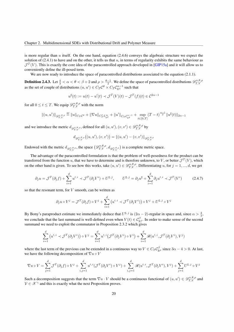
Chapter 2. Multidimensional SDEs with Distributional Drift and Polymer Measure
is more regular than u itself. On the one hand, equation (2.4.6) conveys the algebraic structure we expect thesolution of (2.4.1) to have and on the other, it tells us that u, in terms of regularity exhibits the same behaviour asJ T (V ). This is exactly the core idea of the paracontrolled approach developed in [GIP15a] and it will allow us toconveniently define the ill-posed term.
We are now ready to introduce the space of paracontrolled distributions associated to the equation (2.1.1).
Definition 2.4.3. Let 43 < α < θ < β+2 and ρ > θ−1
2 . We define the space of paracontrolled distributions Dα,θ,ρT,V
as the set of couple of distributions (u, u′) ∈ CTCθ × CTCα−1Rd such that
u♯(t) := u(t)− u′(t) ≺ J T (V )(t)− J T (f)(t) ∈ C2α−1
for all 0 ≤ t ≤ T . We equip Dα,θ,ρT,V with the norm
∥(u, u′)∥Dα,θ,ρT,V
def= ∥u∥CT Cθ + ∥∇u∥Cρ
TL∞Rd
+ ∥u′∥CT Cα−1
Rd+ supt∈[0,T ]
(T − t)α−12 ∥u♯(t)∥2α−1
and we introduce the metric dDα,θ,ρT,V
, defined for all (u, u′), (v, v′) ∈ Dα,θ,ρT,V by
dDα,θ,ρT,V
(u, u′), (v, v′)
= ∥(u, u′)− (v, v′)∥Dα,θ,ρ
T,V
Endowed with the metric dDα,θ,ρT,V
, the spaceDα,θ,ρT,V , dDα,θ,ρ
T,V
is a complete metric space.
The advantage of the paracontrolled formulation is that the problem of well-posedness for the product can betransferred from the function u, that we have to determine and is therefore unknown, to V , or better J T (V ), whichon the other hand is given. To see how this works, take (u, u′) ∈ Dα,θ,ρ
T,V . Differentiating u, for j = 1, ..., d, we get
∂ju = J T (∂jf) +di=1
u′, i ≺ J T (∂jVi) + U ♯, j , U ♯, j = ∂ju
♯ +di=1
∂ju′, i ≺ J T (V i) (2.4.7)
so that the resonant term, for V smooth, can be written as
∂ju V j = J T (∂jf) V j +di=1
u′, i ≺ J T (∂jV
i) V j + U ♯, j V j
By Bony’s paraproduct estimate we immediately deduce that U ♯, j is (2α− 2)-regular in space and, since α > 43 ,
we conclude that the last summand is well-defined even when V (t) ∈ CβRd . In order to make sense of the secondsummand we need to exploit the commutator in Proposition 2.3.2 which gives
di=1
u′, i ≺ J T (∂jV
i) V j =
di=1
u′, iJ T (∂jV
i) V i+
di=1
R(u′, i,J T (∂jVi), V j)
where the last term of the previous can be extended in a continuous way to V ∈ CTCβRd since 3α− 4 > 0. At last,we have the following decomposition of ∇u V
∇u V =dj=1
J T (∂jf) V j +d
i,j=1
u′, i(J T (∂jVi) V j) +
di,j=1
R(u′, i,J T (∂jVi), V j) +
dj=1
U ♯, j V j
Such a decomposition suggests that the term ∇u · V should be a continuous functional of (u, u′) ∈ Dα,θ,ρT,V and
V ∈ X γ and this is exactly what the next Proposition proves.
20
2.4. Solving the Generator equation
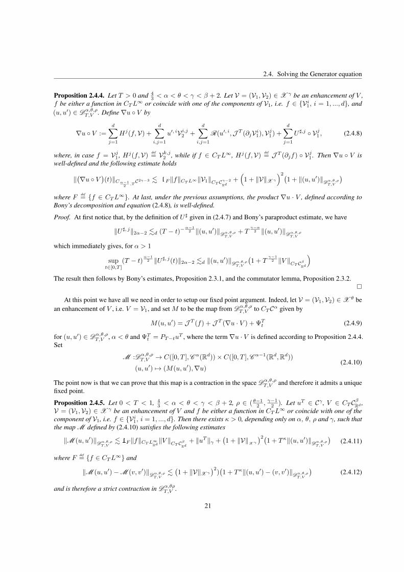
Proposition 2.4.4. Let T > 0 and 43 < α < θ < γ < β + 2. Let V = (V1,V2) ∈ X γ be an enhancement of V ,
f be either a function in CTL∞ or coincide with one of the components of V1, i.e. f ∈ Vi1, i = 1, ..., d, and(u, u′) ∈ Dα,θ,ρ
T,V . Define ∇u V by
∇u V :=dj=1
Hj(f,V) +d
i,j=1
u′, iVi,j2 +d
i,j=1
R(u′, i,J T (∂jVi1),Vj1) +
dj=1
U ♯,j Vj1 , (2.4.8)
where, in case f = Vj1 , Hj(f,V) def= Vk,j2 , while if f ∈ CTL
∞, Hj(f,V) def= J T (∂jf) Vj1 . Then ∇u V is
well-defined and the following estimate holds
∥∇u V
(t)∥Cα−1
2,T
C2γ−3 . 1F ∥f∥CTL∞∥V1∥CT Cγ−2
Rd+1 + ∥V∥X γ
21 + ∥(u, u′)∥Dα,θ,ρ
T,V
where F def
= f ∈ CTL∞. At last, under the previous assumptions, the product ∇u · V , defined according to
Bony’s decomposition and equation (2.4.8), is well-defined.
Proof. At first notice that, by the definition of U ♯ given in (2.4.7) and Bony’s paraproduct estimate, we have
∥U ♯, j∥2α−2 .d (T − t)−α−12 ∥(u, u′)∥Dα,θ,ρ
T,V+ T
γ−α2 ∥(u, u′)∥Dα,θ,ρ
T,V
which immediately gives, for α > 1
supt∈[0,T ]
(T − t)α−12 ∥U ♯, j(t)∥2α−2 .d ∥(u, u′)∥Dα,θ,ρ
T,V
1 + T
γ−12 ∥V ∥CT Cβ
Rd
The result then follows by Bony’s estimates, Proposition 2.3.1, and the commutator lemma, Proposition 2.3.2.
At this point we have all we need in order to setup our fixed point argument. Indeed, let V = (V1,V2) ∈ X θ bean enhancement of V , i.e. V = V1, and set M to be the map from Dα,θ,ρ
T,V to CTCα given by
M(u, u′) = J T (f) + J T (∇u · V ) + ΨTt (2.4.9)
for (u, u′) ∈ Dα,θ,ρT,V , α < θ and ΨTt = PT−tu
T , where the term ∇u · V is defined according to Proposition 2.4.4.Set
M :Dα,θ,ρT,V → C([0, T ],C α(Rd))× C([0, T ],C α−1(Rd,Rd))
(u, u′) →→ (M(u, u′),∇u)(2.4.10)
The point now is that we can prove that this map is a contraction in the space Dα,θ,ρT,V and therefore it admits a unique
fixed point.
Proposition 2.4.5. Let 0 < T < 1, 43 < α < θ < γ < β + 2, ρ ∈ ( θ−1
2 , γ−12 ). Let uT ∈ Cγ , V ∈ CTCβRd ,
V = (V1,V2) ∈ X γ be an enhancement of V and f be either a function in CTL∞ or coincide with one of thecomponent of V1, i.e. f ∈ Vi1, i = 1, ..., d. Then there exists κ > 0, depending only on α, θ, ρ and γ, such thatthe map M defined by (2.4.10) satisfies the following estimates
∥M (u, u′)∥Dα,θ,ρT,V
. 1F ∥f∥CTL∞Rd∥V ∥CT Cβ
Rd+ ∥uT ∥γ +
1 + ∥V∥
X γ
21 + Tκ∥(u, u′)∥Dα,θ,ρ
T,V
(2.4.11)
where F def= f ∈ CTL
∞ and
∥M (u, u′)− M (v, v′)∥Dα,θ,ρT,V
.1 + ∥V∥X γ
2)1 + Tκ∥(u, u′)− (v, v′)∥Dα,θ,ρ
T,V
(2.4.12)
and is therefore a strict contraction in Dα,θρT,V .
21
Chapter 2. Multidimensional SDEs with Distributional Drift and Polymer Measure
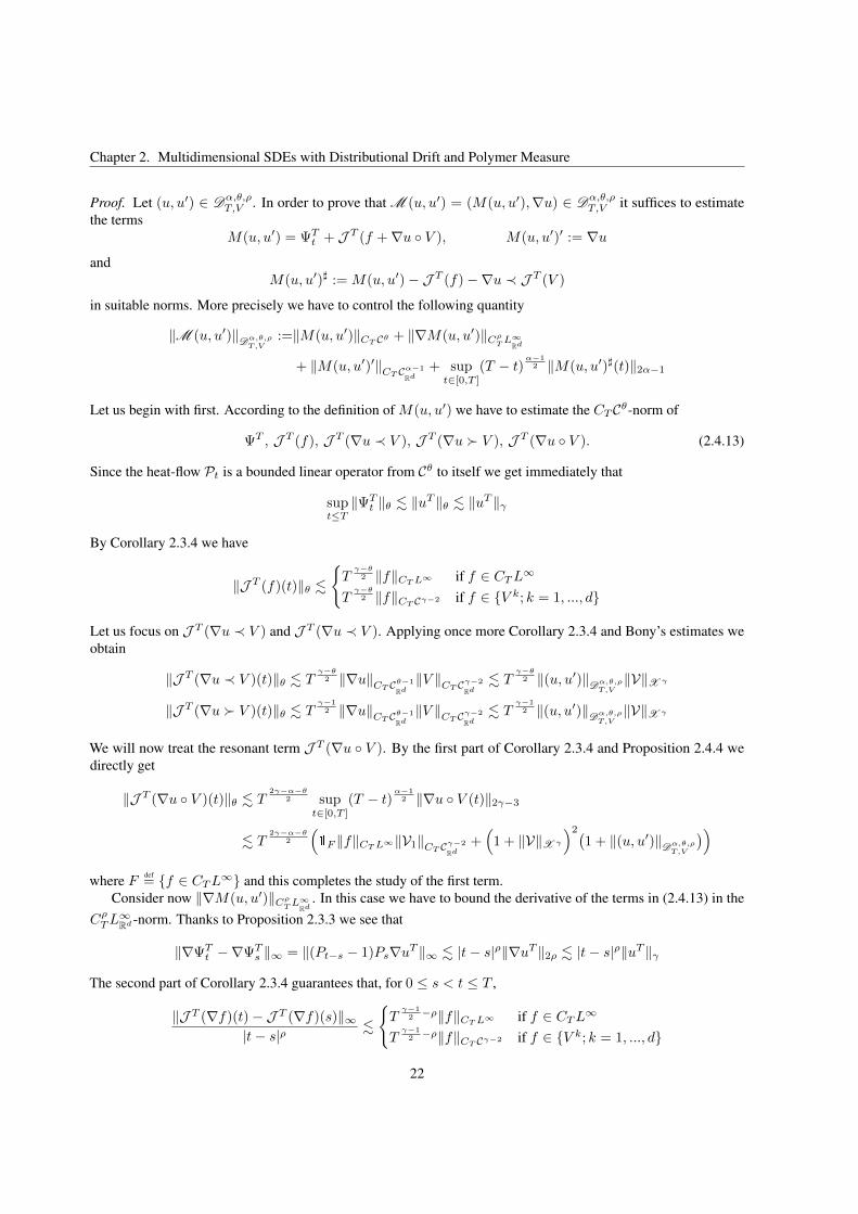
Proof. Let (u, u′) ∈ Dα,θ,ρT,V . In order to prove that M (u, u′) = (M(u, u′),∇u) ∈ Dα,θ,ρ
T,V it suffices to estimatethe terms
M(u, u′) = ΨTt + J T (f +∇u V ), M(u, u′)′ := ∇u
andM(u, u′)♯ :=M(u, u′)− J T (f)−∇u ≺ J T (V )
in suitable norms. More precisely we have to control the following quantity
∥M (u, u′)∥Dα,θ,ρT,V
:=∥M(u, u′)∥CT Cθ + ∥∇M(u, u′)∥CρTL
∞Rd
+ ∥M(u, u′)′∥CT Cα−1
Rd+ supt∈[0,T ]
(T − t)α−12 ∥M(u, u′)♯(t)∥2α−1
Let us begin with first. According to the definition of M(u, u′) we have to estimate the CTCθ-norm of
ΨT , J T (f), J T (∇u ≺ V ), J T (∇u ≻ V ), J T (∇u V ). (2.4.13)
Since the heat-flow Pt is a bounded linear operator from Cθ to itself we get immediately that
supt≤T
∥ΨTt ∥θ . ∥uT ∥θ . ∥uT ∥γ
By Corollary 2.3.4 we have
∥J T (f)(t)∥θ .
T
γ−θ2 ∥f∥CTL∞ if f ∈ CTL
∞
Tγ−θ2 ∥f∥CT Cγ−2 if f ∈ V k; k = 1, ..., d
Let us focus on J T (∇u ≺ V ) and J T (∇u ≺ V ). Applying once more Corollary 2.3.4 and Bony’s estimates weobtain
∥J T (∇u ≺ V )(t)∥θ . Tγ−θ2 ∥∇u∥CT Cθ−1
Rd∥V ∥CT Cγ−2
Rd. T
γ−θ2 ∥(u, u′)∥Dα,θ,ρ
T,V∥V∥X γ
∥J T (∇u ≻ V )(t)∥θ . Tγ−12 ∥∇u∥CT Cθ−1
Rd∥V ∥CT Cγ−2
Rd. T
γ−12 ∥(u, u′)∥Dα,θ,ρ
T,V∥V∥X γ
We will now treat the resonant term J T (∇u V ). By the first part of Corollary 2.3.4 and Proposition 2.4.4 wedirectly get
∥J T (∇u V )(t)∥θ . T2γ−α−θ
2 supt∈[0,T ]
(T − t)α−12 ∥∇u V (t)∥2γ−3
. T2γ−α−θ
2
1F ∥f∥CTL∞∥V1∥CT Cγ−2
Rd+1 + ∥V∥X γ
21 + ∥(u, u′)∥Dα,θ,ρ
T,V
where F def
= f ∈ CTL∞ and this completes the study of the first term.
Consider now ∥∇M(u, u′)∥CρTL
∞Rd
. In this case we have to bound the derivative of the terms in (2.4.13) in theCρTL
∞Rd -norm. Thanks to Proposition 2.3.3 we see that
∥∇ΨTt −∇ΨTs ∥∞ = ∥(Pt−s − 1)Ps∇uT ∥∞ . |t− s|ρ∥∇uT ∥2ρ . |t− s|ρ∥uT ∥γ
The second part of Corollary 2.3.4 guarantees that, for 0 ≤ s < t ≤ T ,
∥J T (∇f)(t)− J T (∇f)(s)∥∞|t− s|ρ
.
T
γ−12 −ρ∥f∥CTL∞ if f ∈ CTL
∞
Tγ−12 −ρ∥f∥CT Cγ−2 if f ∈ V k; k = 1, ..., d
22

2.4. Solving the Generator equation
Analogously, by Bony’s estimates we get
∥J T∇(∇u ≺ V )
(t)− J T
∇(∇u ≺ V )
(s)∥∞
|t− s|ρ. T
γ−12 −ρ∥∇u∥CT Cθ−1
Rd∥V ∥CT Cγ−2
Rd
and∥J T
∇(∇u ≻ V )
(t)− J T
∇(∇u ≻ V )
(s)∥∞
|t− s|ρ. T
θ+γ−22 −ρ∥∇u∥CT Cθ−1
Rd∥V ∥CT Cγ−2
Rd
which in turn imply the correct bound. At last, by Corollary 2.3.4 and Proposition 2.4.4 we have
∥J T∇(∇u V )
(t)− J T
∇(∇u V )
(s)∥∞
|t− s|ρ. T
2γ−2ρ−α2 sup
t∈[0,T ]
(T − t)α−12 ∥∇u V (t)∥2γ−3
T2γ−2ρ−α
2
1F ∥f∥CTL∞∥V1∥CT Cγ−2
Rd+1 + ∥V∥X γ
21 + ∥(u, u′)∥Dα,θ,ρ
T,V
Concerning, the so called Gubinelli derivative, by definition, M(u, u′)′ = ∇u and, by assumption, u ∈ CTCθ.Hence
∥M(u, u′)′∥CT Cα−1
Rd. ∥u∥CT Cα . ∥u∥CT Cθ . ∥(u, u′)∥Dα,θ,ρ
T,V
However this not yet the needed bound due to the missing factor T to some positive power. Let us observe that
∥∇u(t)∥α−1 . ∥∇u(t)−∇u(T )∥α−1 + ∥∇uT ∥α−1 . ∥∇u(t)−∇u(T )∥α−1 + ∥uT ∥α
Now it suffices to notice that we can estimate the first summand in two different ways
∥∆i(∇u(t)−∇u(T ))∥∞ .
2−i(θ−1)∥u∥CT Cθ
(T − t)ρ∥∇u∥CρL∞Rd
where ∆i is the i-th Littlewood-Paley block. Then interpolating this two bounds we get
∥∇u(t)−∇u(T )∥α−1 . T ρ(1−ε)∥u∥εCT Cθ∥∇u∥1−εCρL∞Rd
. T ρ(1−ε)∥(u, u′)∥Dα,θ,ρT,V
with ε := α−1θ−1 ∈ (0, 1). Therefore
∥M(u, u′)′∥CT Cα−1
Rd= ∥∇u∥CT Cα−1
Rd. T ρ(1−ε)∥(u, u′)∥Dα,θ,ρ
T,V+ ∥uT ∥θ
and we can now move to the term involving the remainder M(u, u′)♯. By definition, M(u, u′)♯ is given by
M(u, u′)♯ =M(u, u′)− J T (f)−∇u ≺ J T (V )
= ΨT +J T (∇u ≺ V )−∇u ≺ J T (V )
+ J T (∇u ≻ V ) + J T (∇u V )
Now, by Schauder’s estimates we directly have
(T − t)α−12 ∥ΨT (t)∥2α−1 . (T − t)
γ−α2 ∥uT ∥γ
which gives the needed bound for the term ΨT . Lemma 2.4.2 and the fact that α < θ imply
(T − t)α−12 ∥J T (∇u ≺ V )−∇u ≺ J T (V )∥CT C2α−1
Rd. Tκ(T − t)
α−12
∥u∥CT Cθ + ∥∇u∥Cρ
TL∞Rd
∥V ∥CT Cγ
Rd
23
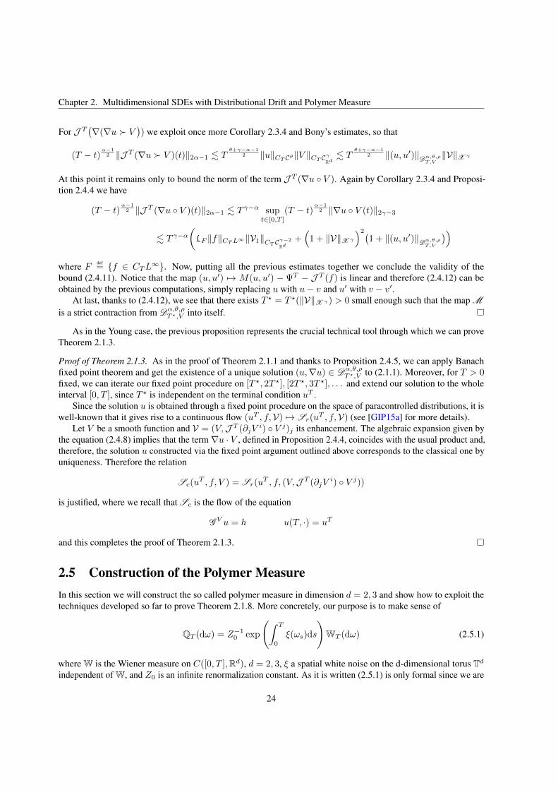
Chapter 2. Multidimensional SDEs with Distributional Drift and Polymer Measure
For J T∇(∇u ≻ V
) we exploit once more Corollary 2.3.4 and Bony’s estimates, so that
(T − t)α−12 ∥J T (∇u ≻ V )(t)∥2α−1 . T
θ+γ−α−12 ∥u∥CT Cθ∥V ∥CT Cγ
Rd. T
θ+γ−α−12 ∥(u, u′)∥Dα,θ,ρ
T,V∥V∥X γ
At this point it remains only to bound the norm of the term J T (∇u V ). Again by Corollary 2.3.4 and Proposi-tion 2.4.4 we have
(T − t)α−12 ∥J T (∇u V )(t)∥2α−1 . T γ−α sup
t∈[0,T ]
(T − t)α−12 ∥∇u V (t)∥2γ−3
. T γ−α1F ∥f∥CTL∞∥V1∥CT Cγ−2
Rd+1 + ∥V∥X γ
21 + ∥(u, u′)∥Dα,θ,ρ
T,V
where F def
= f ∈ CTL∞. Now, putting all the previous estimates together we conclude the validity of the
bound (2.4.11). Notice that the map (u, u′) →→ M(u, u′) − ΨT − J T (f) is linear and therefore (2.4.12) can beobtained by the previous computations, simply replacing u with u− v and u′ with v − v′.
At last, thanks to (2.4.12), we see that there exists T ⋆ = T ⋆(∥V∥X γ ) > 0 small enough such that the map M
is a strict contraction from Dα,θ,ρT⋆,V into itself.
As in the Young case, the previous proposition represents the crucial technical tool through which we can proveTheorem 2.1.3.
Proof of Theorem 2.1.3. As in the proof of Theorem 2.1.1 and thanks to Proposition 2.4.5, we can apply Banachfixed point theorem and get the existence of a unique solution (u,∇u) ∈ Dα,θ,ρ
T⋆,V to (2.1.1). Moreover, for T > 0fixed, we can iterate our fixed point procedure on [T ⋆, 2T ⋆], [2T ⋆, 3T ⋆], . . . and extend our solution to the wholeinterval [0, T ], since T ⋆ is independent on the terminal condition uT .
Since the solution u is obtained through a fixed point procedure on the space of paracontrolled distributions, it iswell-known that it gives rise to a continuous flow (uT , f,V) →→ Sr(u
T , f,V) (see [GIP15a] for more details).Let V be a smooth function and V = (V,J T (∂jV
i) V j)j its enhancement. The algebraic expansion given bythe equation (2.4.8) implies that the term ∇u · V , defined in Proposition 2.4.4, coincides with the usual product and,therefore, the solution u constructed via the fixed point argument outlined above corresponds to the classical one byuniqueness. Therefore the relation
Sc(uT , f, V ) = Sr(u
T , f, (V,J T (∂jVi) V j))
is justified, where we recall that Sc is the flow of the equation
G V u = h u(T, ·) = uT
and this completes the proof of Theorem 2.1.3.
2.5 Construction of the Polymer MeasureIn this section we will construct the so called polymer measure in dimension d = 2, 3 and show how to exploit thetechniques developed so far to prove Theorem 2.1.8. More concretely, our purpose is to make sense of
QT (dω) = Z−10 exp
T
0
ξ(ωs)ds
WT (dω) (2.5.1)
where W is the Wiener measure on C([0, T ],Rd), d = 2, 3, ξ a spatial white noise on the d-dimensional torus Tdindependent of W, and Z0 is an infinite renormalization constant. As it is written (2.5.1) is only formal since we are
24
2.5. Construction of the Polymer Measure
exponentiating the integral in time of a white noise, which is a distribution, over a Brownian path and dividing thenby an infinite constant, all operations that require to be given a meaning to.
To this aim, let ξε be a mollification of ξ with mollifier m, as in (2.1.3), Qε the measure defined by
QεT (dω) = Z−1ε exp
T
0
ξε(ωs)ds
W(dω), Zε = EW
exp
T
0
ξε(ωs)ds
and hε : R+ × Td → R be the local in time solution to the equation
∂thε =
1
2∆hε +
1
2|∇hε|2 + ξε − cε h(0, x) = 0 (2.5.2)
where cε is a diverging constant that will be characterized in Theorem 2.6.12. For ξε smooth, hε is known to existand be regular, therefore the process
Mεt (ωs) =
t
0
∇hε(T − s, ωs)dωs with quadratic variation ⟨Mε⟩t(ω) = t
0
|∇hε(T − s, ωs)|2ds
is clearly a square integrable martingale. Girsanov’s theorem then implies that, under the measure defined by
QεT (dω) = exp
MεT − 1
2⟨Mε⟩T
W(dω),
the canonical process has the same law as the solution Xε to the SDE
dXεt = V ε(t,Xε
t )dt+ dBt, X0 = x
when one chooses V ε(t, x) to be ∇hε(T − t, x). But now, applying Ito’s formula to hε(T − t,Xεt ) and recalling
that hε solves (2.5.2) we conlude that QεT (dω) = QεT (dω).At this point we can take advantage of Theorem 2.1.7, whose applicability is ensured by the next proposition,
which guarantees the existence of a unique limiting measure for the sequence (QεT )ε and consequently for thesequence (QεT )ε.
Proposition 2.5.1. Let hε be the local in time solution to (2.5.2) for d = 2, 3 and V ε(t, x) = ∇hε(T − t, x). Then,there exists T ⋆ > 0 such that for all T ≤ T ⋆, V ε(t, x) is a ground drift according to definition 2.1.5, i.e. we have
1. For d = 2 the process V ε converges almost surely in C([0, T ⋆], Cβ(T2)) for all β < 0 to some element V .
2. For d = 3 and all β < −1/2 the process K(V ε) converges almost surely in H β+2(T3) to some elementV ∈ X β+2.
Moreover in both cases the limit is independent of the choice of the mollifier f .
Remark 2.5.2. Notice that we are applying Theorem 2.1.7 to distributions defined on the torus and not on the fullspace. This is completely harmless since the space Cγ(Td) can be seen as the space of periodic distributions lyingin Cγ (see also [GIP15a, Appendix A] for a discussion of this aspect).
Let us stress the fact that the proof of Proposition 2.5.1 boils down to a well-posedness result for the equation
∂th =1
2∆h+
1
2|∇h|2 + ξ, h(0, x) = 0. (2.5.3)
In the one dimensional case with ξ a space-time white noise, the previous is nothing but the celebrated Kardar-Parisi-Zhang equation [KPZ86], which was successfully studied by M.Hairer in [Hai13] and subsequently by M. Gubinelliand N.Perkowski in [GP15]. The regularity issues one encounters when dealing with the three dimensional versionare morally the same these authors had to face and the techniques we will exploit are somewhat similar to theirs(especially to [GP15]). For the sake of completeness, we will still prove 2.5.1 pointing out the difficulties one has toovercome and illustrating the main steps one needs to undertake in order to solve (2.5.3), still keeping it as conciseas possible and referring the interested reader to the quoted papers.
25
Chapter 2. Multidimensional SDEs with Distributional Drift and Polymer Measure
2.6 A KPZ-type equation driven by a purely spatial white noiseThe aim of this section is to prove well-posedness of the KPZ-type equation, introduced in (2.5.3) to make sense ofthe polymer measure with white-noise potential. We will focus on the three-dimensional case, since in dimension 2the result follows by analogous, but simpler, arguments.
Let us consider the case of non-zero initial condition, h0, and write (2.5.3) in its mild formulation
h(t) = Pth0 + I(|∇h|2)(t) + I(ξ)t (2.6.1)
where Ptdef= e
12 t∆ is the heat flow, for a function f on (0, T ] × T3, I(f)(t) def
= t0Pt−sf(s)ds and ξ is the usual
space white noise on T3, i.e. a centered gaussian random field whose covariance function is formally given asin (2.1.2).
The problem with the previous equation lies on the fact that, since as a random distribution, ξ ∈ Cθ(Td) forθ < −d
2 (which in d = 2 means θ < −1 while in d = 3, θ < − 32 ) stantard Schauder’s estimates suggest that the
spatial regularity of h cannot be better than θ + 2 and therefore the non-linearity in (2.6.1), for both d = 2 and 3,is not well-defined. Now, let us point out that the term determining the regularity of h is I(ξ), so maybe, uponsubtracting it to the potential solution, what remains is more regular. In other words, one defines h1
def= h− I(ξ),
derivates the equation it should solve and, as before, guesses its regularity. For example, setting X = I(ξ), h1should satisfy
h1(t) = Pth0 + I(|∇X|2)(t) + I(∇X · ∇h1 + |∇h1|2)(t)
and its regularity should be as the one of I(|∇X|2). If it were well-posed, this last term would be 2θ + 4-Holder inspace which is strictly greater than θ + 2 so that indeed h1 is more regular than h. While in dimension 2 this isenough (given that X and I(|∇X|2) can be constructed and belong to the correct Besov-Holder space, all the otherterms satisfy Bony’s condition), it is still not sufficient in d = 3 and so, we proceed further in the expansion.
The problem is that after subtracting a finite number of terms, there will be no more gain in regularity andsomething else is needed in order to define the ill-posed product and consequently solve the equation. This is exactlythe point in which the paracontrolled approach, as we will see in what follows, enters the game.
Now that we have given a heuristic idea of what is going on, let us be more formal. We begin by defining theobjects that will appear in our expansion. Let η be a smooth function and set
Xt(η)def= I(η)(t), Xt (η)
def= I(|∇X|2)(t), Xt (η)
def= I(∇X · ∇X)(t),
Xt (η)def= I(∇X · ∇X)(t), Xt (η)
def= I(|∇X |2)(t).
(2.6.2)
As announced before, in case η is the space white noise, the previous stochastic processes are not analiticallywell-defined and we will have to exploit stochastic calculus tools in order to make sense of them and prove that theysatisfy certain regularity requirements.
Now, let h be the solution of (2.6.1) driven by η and v be given by
vdef= h−X(η)−X (η)− 2X (η) .
Plugging this expression back into (2.6.1), we see that v solves
v(t) = Pth0 + 4Xt (η) + 2 I∇v · ∇X(η)
(t) +Rv(t) (2.6.3)
where Rv is defined as
Rv(t) := Xt (η) + I2∇X (η) · ∇
2X (η) + v
+∇2X (η) + v
2(t) (2.6.4)
26
2.6. A KPZ-type equation driven by a purely spatial white noise
At this point, we will split the analysis of the equation in two distinct modules. On one side, with purely analyticalarguments, we will identify a suitable subspace of the space of distributions, depending on the processes definedabove, for which it is possible to make sense of the ill-posed operations in (2.6.3) and formulate a fixed point mapthat is continuous in these data. On the other, we will exploit probabilistic techniques to construct such processesstarting with a white noise ξ and prove they have the expected regularity, through a regularization procedure.
Notation. From now on, all the functions and distributions we will consider will live on the d-dimensionaltorus. Since no confusion can occur, we will indicate the function spaces with the same notations introduced inSection 2.0.1, but the domain will not be Rd but Td.
2.6.1 Analytic partWe begin by specifying the space in which our stochastic processes live.
Definition 2.6.1 (Rough Distribution). Let ϱ, r < 12 be such that ϱ + 2r < 1
2 . For (a, b, η) ∈ R2 × CTC2 andt ≤ T set X(η, a, b) to be
Xt(η, a, b) =Xt, Xt − at,Xt , Xt , Xt − bt,Q ∇X(t)
(η) (2.6.5)
where X , X , X , X are given by (2.6.2), and
Q(η)def= I(∇X) and ∇Q ∇X(η) = (∂i(Q)j ∂iX)i,j=1,2,3.
We define the space X ϱ,r of rough distributions as
X ϱ,r = clHϱ,r
X(η, a, b), (a, b, η) ∈ R2 × C([0, T ],C 2(T3))
where clHϱ,r· denotes the closure of the set in brackets with respect to the topology of Hϱ,r and the spaceHϱ,r = CrTCϱ × CrTC2ϱ × CrTC3ϱ × CrTCϱ+1 × CrTC4ϱ × CrTC
2ϱ−1R3 equipped with its usual norm. We will denote
by X a generic 6-uple given as in 2.6.5 belonging to this space. Moreover if η ∈ CTCϱ coincides with the firstcomponent of X ∈ X ϱ,r we will say that X is a enhancement (or lift) of η.
Remark 2.6.2. The reason why in (2.6.5) we had to add an extra term to ones introduced in (2.6.2) will soonbe clarified. Intuitively, this is the term we will need to define the ill-posed product between the gradient of theexpected solution v of (2.6.3) and the grandient of X . This is very similar to what done for the generator equationin Section 2.4.2.
Remark 2.6.3. It is important to notice that the two constants a, b appearing in Definition 2.6.1 play the role ofrenormalization constants. As we said at the beginning of section 2.6, if ξ denotes the three dimensional spacewhite noise, then there is simply no hope to define some of the terms of X(ξ) as the limit of smooth approximations.However, we will see that, upon subtracting suitable diverging constants, it is still possible to obtain a nontriviallimit. To exemplify, for X , if Xε a mollification of X , then I(|∇Xε|2)(t) does not converge, but there exists adiverging sequence of cε such that I(|∇Xε|2)(t)− cεt indeed does (see Theorem 2.6.12 for a complete proof).
Remark 2.6.4. One of the main differences with the KPZ equation studied in [Hai13] and [GP15] is the stochastic
term X . Indeed, while in the latter case this term requires a non trivial renormalization, in our it does not (seeagain Theorem 2.6.12).
Given X ∈ X ϱ,r, ϱ < 12 , the goal of this section is to setup a fixed point argument for equation (2.6.3). Now,
from the definition of X we see that the expected spatial regularity of the solution v should be ϱ+ 1 and not betterso that all the terms are well-defined, thanks to Proposition 2.3.1, with the exception of ∇v · ∇X , and, in particular,the resonant part of it. This difficulty can be handled in the same way as in Section 2.4.2, namely we will exploitonce more the idea of paracontrolled distributions introduced in [GIP15a].
27
Chapter 2. Multidimensional SDEs with Distributional Drift and Polymer Measure
Definition 2.6.5 (Paracontrolled Distributions). Let 25 < α < 1
2 . For Q ∈ CTCα+1, we define the space ofparacontrolled distributions Dα
Q,T as the set of couple of functions (v, v′) ∈ CTCα+1 × CTCαR3 such that
v♯(t)def= v(t)− (v′ ≺ Q)(t) ∈ C4α
for all 0 ≤ t ≤ T . We equip DαQ,T with the norm
∥(v, v′)∥DαQ,T
= ∥v∥1 + ∥v′∥2 + ∥v♯∥3
where, for β ∈ (0, 3α− 1), γ ∈ (2α, α+ 12 ), δ ∈ (2α− 1
2 , α), the norms ∥ · ∥i, i = 1, 2, 3 are defined by
∥v∥1def= ∥v∥1,x + ∥v∥1,T
def= supt∈[0,T ]
tα2 ∥v(t)∥3α + sup
0≤s<t≤Ts
1+δ−α2
∥∇v(t)−∇v(s)∥L∞
|t− s| δ2
∥v′∥2def= supt∈[0,T ]
tγ2 ∥v′(t)∥3α−1 ∥v♯∥3
def= supt∈[0,T ]
tβ+12 ∥v♯(t)∥α+β+1
For (u, u′) ∈ DαQ,T , we say that u is paracontrolled by Q and we endow Dα
Q,T with the metric
dDαQ,T
((v1, v′1), (v2, v
′2)) := ∥v1 − v2∥1 + ∥v′1 − v′2∥2 + ∥v♯1 − v♯2∥3
for (v1, v′1), (v2, v′2) ∈ Dα
Q,T .
At this point let (v, v′) ∈ DαQ,T . Then, upon decomposing the product in the paraproduct and resonant part, and
exploiting the paracontrolled structure of v, we can write ∇X ∇v as
∇X ∇v = ∇X ∇(v′ ≺ Q) +∇X ∇v♯
= ∇X (∇v′ ≺ Q) +∇X (v′ ≺ ∇Q) +∇X ∇v♯
where, thanks to Bony’s estimates and since α > 25 , all the terms are well-defined apart from the second summand.
But now thanks to the commutator lemma, Proposition 2.3.2, we have
∇X ∇v = ∇X (∇v′ ≺ Q) 5α−2
+ v′(∇X ∇Q) 2α−1
+R(v′,∇X,∇Q) 2α−1
+∇X ∇v♯ 5α−2
(2.6.6)
Provided we can make sense of ∇Q ∇X through other means, the resonant term is now well posed and has spatialregularity given by 2α− 1. In the next proposition, we will derive suitable estimates for the convolution of the latterwith the heat kernel, which is exactly what we need in the proof of the fixed point (see Proposition 2.6.8).
Proposition 2.6.6. Let 25 < α < ϱ < 1
2 , X ∈ X ϱ,r, v ∈ DαQ,T and assume ∇Q ∇X is well-defined and belongs
to CTC2α−1. Then ∇X ∇v is well-posed and is given by the expansion in (2.6.6). Moreover, when convolvedwith the heat kernel, it satisfies the following estimateI∇X ∇v
1+I∇X ∇v
3. Tϑ∥X∥Xϱ,r
1 + ∥X∥Xϱ,r
∥v′∥2 + ∥v♯∥3
(2.6.7)
where ϑ = 1+δ−α−γ2 > 0 and ∥ · ∥i, for i = 1, 2, 3, are defined as in Definition 2.6.5.
Proof. The argument above justifies the expansion we made and guarantees the well-posedness of the resonant term.In order to obtain the required bounds it is sufficient to apply Corollary 2.3.4, Bony’s estimates (Proposition 2.3.1)and the commutator Lemma (Proposition 2.3.2). Indeed,I∇X ∇v
1,x
. T4α−γ
2 supss
γ2 ∥∇Xs (∇v′s ≺ Qs)∥5α−2 + T
α+1−γ2 sup
ss
γ2 ∥v′(s)(∇X ∇Q)s∥2α−1
+ Tα+1−γ
2 supss
γ2 ∥C(v′,∇X,∇Q)(s)∥2α−1 + T
α−β2 sup
ss
β+12 ∥∇Xs ∇v♯(s)∥5α−2
. Tα−β
2 ∥X∥Xϱ
1 + ∥X∥Xϱ
sups
s
γ2 ∥v′(s)∥3α−1 + s
β+12 ∥v♯(s)∥α+β+1
28
2.6. A KPZ-type equation driven by a purely spatial white noise
andI∇X ∇v
3. T
4α−γ2 sup
ss
γ2 ∥∇Xs (∇v′s ≺ Qs)∥5α−2 + T
α+1−γ2 sup
ss
γ2 ∥v′(s)(∇X ∇Q)s∥2α−1
+ Tα+1−γ
2 supss
γ2 ∥C(v′,∇X,∇Q)(s)∥2α−1 + T
4α−β−12 sup
ss
β+12 ∥∇Xs ∇v♯(s)∥5α−2
. T4α−β−1
2 ∥X∥Xϱ,0
1 + ∥X∥Xϱ,0
sups
s
γ2 ∥u′(s)∥3α−1 + s
β+12 ∥u♯(s)∥α+β+1
where, in both cases, the first inequality follows by Corollary 2.3.4 part 1, and the second by Propositions 2.3.1 and2.3.2. As before,I∇X ∇v
1,T
. T1+δ−α−γ
2
supss
γ2 ∥∇Xs (∇v′s ≺ Qs)∥5α−2 + sup
ss
γ2 ∥v′(s)(∇X ∇Q)s∥2α−1
+ supss
γ2 ∥C(v′,∇X,∇Q)(s)∥2α−1 + sup
ss
β+12 ∥∇Xs ∇v♯(s)∥5α−2
. T
1+δ−α−γ2 ∥X∥Xϱ,0
1 + ∥X∥Xϱ,0
sups
s
γ2 ∥v′(s)∥3α−1 + s
β+12 ∥v♯(s)∥α+β+1
but we apply the second part of Corollary 2.3.4 instead of the first. Since 1+δ−α−γ
2 < min 4α−β−12 , α−β2 the
conclusion follows.
At this point we need to indentify v′, Q and v♯ so that we can establish a fixed point map in the space ofparacontrolled distributions. To do so, let (v, v′) ∈ Dα
Q,T and notice that v solves (2.6.3) if and only if v♯ solves
v♯(t) = Pt(u0 − v′ ≺ Q(0)) + I∇4X + 2v) ≺ ∇X
(t)− v′ ≺ Q(t)
+ 2 I∇v ∇X
(t)
+Rv(t)
where Rv was introduced in (2.6.4). Now, we expect v♯ to have spatial regularity greater than the one of v but allthe terms in the first line, not involving the initial condition have regularity α+ 1 and not better. The point here is totake advantage of the difference and prove it is more regular than each of its summands. As the next Propositionshows, this is indeed the case upon choosing v′ and Q wisely.
Proposition 2.6.7. Let α, β, γ and δ be as in Definition 2.6.5. Let X ∈ X ϱ,r, for 25 < α < ϱ < 1
2 , and f be suchthat
∥f∥⋆ = ∥f∥⋆,T + ∥f∥2def= ∥f∥C3α−1
1+δ−α,TL∞ + ∥f ′∥Cγ,T C3α−1
R3<∞
then∥I(f ≺ ∇X)− f ≺ I(∇X)∥3 . T
4α−1−δ2 ∥f∥⋆∥X∥ϱ (2.6.8)
Proof. Let us rewrite the left hand side of (2.6.8) as
tβ+12 ∥I(f ≺ ∇X)(t)− f(t) ≺ I(∇X)(t)∥α+β+1 ≤
tβ+12
t
0
Pt−s(f(s)− f(t)) ≺ ∇Xs
α+β+1
ds+ (2.6.9)
tβ+12
t
0
Pt−s(f(t) ≺ ∇Xs)ds− f(t) ≺ Pt−s∇Xs
α+β+1
ds (2.6.10)
29
Chapter 2. Multidimensional SDEs with Distributional Drift and Polymer Measure
Let us consider the two summands separately. Thanks to Proposition 2.3.3, (2.6.9) is bounded by
tβ+12
t
0
(t− s)−1− β2 ∥f(s)− f(t)∥L∞ds∥X∥α ≤ t
β+12
t
0
(t− s)−1− β2 + 3α−1
2 s−1+δ−α
2 ds∥f∥⋆,T ∥X∥α
≤ T4α−1−δ
2 ∥f∥⋆,T ∥X∥ϱ
where we used the fact that β < 3α− 1 and δ < α < ϱ.For (2.6.10) we apply the commutator (2.3.1) in Proposition 2.3.3, so that we obtain
tβ+12
t
0
(t− s)−3−3α+β
2 ds∥f(t)∥3α−1∥X∥α . tβ+1−γ
2
t
0
(t− s)−3−3α+β
2 ds∥f∥2∥X∥α
≤ T3α−γ
2 ∥f∥2∥X∥ϱ
the last passage being justified by the fact that β < 3α− 1. Since 2α− 12 < δ we obtain (2.6.8).
Proposition 2.6.7 conveys that if we take
Qt := I(∇X)(t)
v′ := 2∇v + 4∇X
we should be in business, i.e. we should be able to determine a fixed point map in the space of paracontrolleddistributions Dα
Q,T .So far we have put all the elements in place and we have now the tools we need in order to prove that, for a
given rough distribution X ∈ X ϱ,r, equation (2.6.3) has a unique local in time solution.
Proposition 2.6.8. Let α, ϱ ∈ ( 25 ,12 ) with α < ϱ. Let X ∈ X ϱ,r and h0 ∈ Cα. For (v, v′) ∈ Dα
Q,T , letG : Dα
Q,T → CTCα+1 × CTCαR3 be the map defined by G(v, v′) = (v, v′),
vdef= Pth0 + 4Xt + 2 I
∇v · ∇X
(t) +Rv(t), v′
def= 2∇v + 4∇X
where the product term has to be understood according to Proposition 2.6.6 (see the expansion (2.6.6)) and Rv isdefined by (2.6.4). Then G(v, v′) ∈ Dα
Q,T and there exists ϑ > 0 such that
∥G (v, v′)∥DαQ,T
.1 + ∥X∥Xϱ,r + ∥h0∥α
21 + Tϑ∥(v, v′)∥Dα
Q,T
2(2.6.11)
and, for V1 = (v1, v′1), V2 = (v2, v
′2) ∈ Dα
Q,T ,
dDαQ,T
G (V1),G (V2)
. TϑdDα
Q,T(V1, V2)
1 + ∥V1∥Dα
Q,T+ ∥V2∥Dα
Q,T
1 + ∥X∥Xϱ,r
2(2.6.12)
Proof. As already pointed out, G (v, v′) has indeed the algebraic structure of a distribution paracontrolled by Qonce we set
v′ = 2∇v + 4∇X
v♯ = PthQ0 + I
v′ ≺ ∇X
(t)− v′ ≺ Q(t) + 2 I
∇v ∇X
(t) + Rv(t)
In order to obtain the bound (2.6.11), let us separately consider each term. Let us begin with ∥v′∥2.
tγ2 ∥v′(t)∥3α−1 . t
γ2
∥v(t)∥3α + ∥X ∥3α
. T
γ−2α2 ∥v∥1,x + t
γ2 ∥X∥Xϱ,r (2.6.13)
30
2.6. A KPZ-type equation driven by a purely spatial white noise
For ∥v♯∥3, set Ii(t), i = 1, . . . , 4 to be the corresponding summand in the definition of v♯, where I2 is the difference,so that
tβ+12 ∥v♯(t)∥α+β+1 .
4i=1
tβ+12 ∥Ii(t)∥α+β+1
Now, as a trivial consequence of Proposition 2.3.3 and since, by definition, Q0 = 0 , we have
tβ+12 ∥I1(t)∥α+β+1 = t
β+12 ∥Pth0∥α+β+1 . ∥h0∥α
For I2, Proposition 2.6.7 tells us that
tβ+12 ∥I2(t)∥α+β+1 . T
4α−1−δ2
∥v′∥⋆,T + ∥v′∥2
∥X∥Xϱ,r
It remains to prove that ∥v′∥⋆,T can be bounded in terms of ∥v∥DαQ,T
((2.6.13) is taking care of ∥v′∥2). But now
∥v′∥⋆,T = sup0≤s<t≤T
s1+δ−α
2∥v′(t)− v′(s)∥∞
|t− s| 3α−12
. sup0≤s<t≤T
s1+δ−α
2∥∇v(t)−∇v(s)∥∞
|t− s| 3α−12
+ s1+δ−α
2 ∥∇X ∥C
3α−12
T L∞. T
δ+1−3α2 ∥v∥1,T + ∥X∥Xϱ,r
I3 is covered by Proposition 2.6.6, while for I4 we have
tβ+12 ∥I4(t)∥α+β+1 . t
β+12 ∥X∥Xϱ + T
1−α2 sup
ssα∥∇v(s) ≻ ∇Xs∥2α−1
+ Tα+1−γ
2 supss
γ2 ∥∇Xs · v′(s)∥2α−1 + T
2α−2γ+12 sup
ssγ∥v′(s)∥23α−1
.1 + ∥X∥Xϱ,r
21 + T
2α−2γ+12 ∥v(s)∥1,x
2where the first inequality follows by Corollary 2.3.4 while the second by Bony’s estimate (Proposition 2.3.1) and(2.6.13). Hence, collecting the bounds obtained so far, we conclude that ∥v♯∥3 satisfies (2.6.11).
By analogous arguments, we proceed with ∥v∥1,x. Corollary 2.3.4 implies
tα∥v(t)∥3α .∥h0∥α + tα∥X∥Xϱ,r + T1−2α
2 supssα∥∇v(s) ≺ ∇Xs∥α−1 +
I∇v ∇X(t)1,x
+ T1−α2 sup
ssα∥∇v(s) ≻ ∇Xs∥2α−1 + T
α+1−γ2 sup
ss
γ2 ∥∇Xs · v′(s)∥2α−1
+ T2α+1−2γ
2 supssγ∥v′(s)∥23α−1
while Proposition 2.6.6 takes care of the resonant term, Proposition 2.3.1 and (2.6.13) allow us to conclude that∥v∥1,x satsfies (2.6.11) for ϑ = α−β
2 .
Finally, let us bound the last norm. Let 0 ≤ s < t ≤ T . At first, notice that a straightforward application ofProposition 2.3.3 gives
s1+δ−α
2∥Pt∇h0 − Ps∇h0∥∞
|t− s| δ2= s
1+δ−α2
∥Pt−s − Id
Ps∇h0∥∞
|t− s| δ2. ∥h0∥α
31
Chapter 2. Multidimensional SDEs with Distributional Drift and Polymer Measure
then, using the fact that Pt and ∇ commute and the second part of Corollary 2.3.4 we have
s1+δ−α
2∥∇v(t)−∇v(s)∥∞
|t− s| δ2. ∥h0∥α + s
1+δ−α2 ∥X∥Xϱ + T
1+δ−α−γ2 sup
ssγ∥v′(s)∥23α−1
+ s1+δ−α
2
∥I∇∇v · ∇X
(t)− I
∇∇v · ∇X
(s)∥∞
|t− s| δ2+ T
1+δ−α−γ2 sup
ss
γ2 ∥∇Xs · v′(s)∥2α−1
Now, Proposition 2.6.6 deals with the resonant term, while the paraproducts can be bounded by
s1+δ−α
2
∥I∇∇v ≺≻ ∇X
(t)− I
∇∇v ≺≻ ∇X
(s)∥∞
|t− s| δ2. T
1−3α+δ2 sup
ss
α2 ∥∇v(s) ≺ ∇Xs∥α−1
+ T1−3α+δ
2 supss
α2 ∥∇v(s) ≻ ∇Xs∥2α−1
where we used the more compact notation f ≺≻ gdef= f ≺ g + f ≻ g. Arguing as before we conclude that (2.6.11)
holds true. The second bound in the statement can be obtained analogously.
Summarizing what achieved so far, we have the following statement.
Theorem 2.6.9. Let 25 < α < ϱ < 1
2 , η ∈ C∞ and let ScKPZ : C2 ×R → C([0,+∞), C2) be the classical flow ofthe equation
∂th(t, x) =1
2∆h(t, x) +
1
2|∇h(t, x)|2 + η(x)− (a+ b), h(0, x) = 0 (2.6.14)
(t, x) ∈ [0,+∞[×T3. Then there exist a lower semi-continuous time T ⋆ : X ϱ,r × R → (0,+∞] and a uniquelocally Lipschitz map SrKPZ : X ϱ,r → C([0,∞[, Cα) such that SrKPZ extends ScKPZ in the following sense
SrKPZ (X(η, a, b)) (t) = ScKPZ(η, a+ b)(t)
for all t ≤ T ⋆(X(η, a, b)) and (η, a, b) ∈ C∞ × R2.
Proof. Given the bounds in Proposition 2.6.8, the proof is completely analogous to the one of Theorem 2.1.3provided in Section 2.4.2.
Remark 2.6.10. The fact that the equation (2.6.14) is globally well-posed, i.e. its solution h does not explode infinite time, when η is a smooth function is ensured by the fact that, thanks to the Cole-Hopf transform, eh is thesolution of the linear equation
∂teh =
1
2∆eh + ehη
which is known to admit a unique global strictly positive solution when the initial condition is identically equal to 1(for example by Feynmann-Kac formula).
Remark 2.6.11. As we pointed out at the beginning of this section, we notice that in d = 2, the space whitenoise belongs to Cη for η < −1, and that an expansion of order one is sufficient in order to make sense of theequation (2.5.2). Moreover in this case the map SrKPZ is simply a locally Lipschitz functional of (X,X )(η).
32
2.6. A KPZ-type equation driven by a purely spatial white noise
2.6.2 Stochastic partLet ξ be a space white noise on T3 and ξε its regularization as in Theorem 2.1.8, i.e.
ξε(x) =k∈Z3
0
m(εk)ξ(k)eik·x (2.6.15)
where m is a smooth radial function with compact support such that m(0) = 1 and (ξ(k))k is a family of gaussianrandom variables with covariance structure given by
E[ξ(k1)ξ(k2)] = 1k1=−k2
In order to complete the study of equation (2.5.3) we have to prove that the process X = I(ξ) can be indeed liftedto the space of rough distributions X ϱ,r. To do so, we will show that, upon defining the processes Xε, Xε, , Xε, ,
Xε, , Xε, ,∇Qε ∇Xε according to (2.6.2) and Definition 2.6.1, we have the following theorem.
Theorem 2.6.12. Let ϱ < 12 and (Ω,F ,Pξ) be a probability space on which the space white noise ξ is defined. Let
m be a smooth radial function with compact support such that m(0) = 1 and ξε be defined as in (2.6.15). Then,upon choosing the constants cε , cε ∈ R as
cε =k =0
|m(εk)|2
|k|2, cε = 2
k1,k2
m(εk1)2m(εk2)
2 |k1 · k2|2
|k12|2|k1|4|k2|4(2.6.16)
the sequence
Xεt :=
Xεt , X
ε,t − cε t,X
ε,t , Xε,
t , Xε,t − cε t,∇Qε ∇Xε(x)
converges to a process X = (X , X , X , X , X ,∇Q ∇X) ∈ Hϱ in Lp(Ω,Hϱ) for every p > 1. Thelimiting process X is independent of the choice of the mollifier and of the sequence of constants cε , cε .
Moreover, replacing ξε with δξε for δ > 0, the corresponding renormalizing constants are such that cε,δ = δ2cε ,
cε,δ = δ4cε .
Remark 2.6.13. The choice of the constants made in (2.6.16) is not unique. Clearly, being them diverging, addingany real number would not prevent the sequence Xε from converging to X. What instead is unique, is their behaviouras ε goes to 0 and it is possible to prove that they asimptotically satisfy
cε ∼ ε−1, cε = O((log(ε))2)
The proof of results of the type of Theorem 2.6.12 makes always use of the same tools (see [GIP15a, CC13,GP15]) and follows a, by now, standard procedure. For τ ∈ ·, , , , , at first one obtains L2 boundson Xε,τ
s,t − Xε′,τs,t , where Xs,t := Xt − Xs, and then the conclusion is attained thanks to Besov embedding
(Proposition (2.0.2)) and Garsia-Rodemich-Rumsey lemma (see [GRR70]). We will prove only the L2 estimates forthe time increment of the mollified processes addressing the interested reader to the relevant literature mentionedabove.
Notation. Since we will run into long formulas, we reckon convenient to introduce some notations we will exploitin the rest of the chapter. As already pointed out, the time increment of a process X will be abbreviated asXs,t := Xt −Xs and for a function of time f(·) we will write f(s, t) := f(t) − f(s). For vectors k1, k2 ∈ Rd,we will indicate by k12 := k1 + k2, by k1 · k2 their scalar product and k1 k⋆2 ∈ Rd×d the matrix generated by thecolumn by vector product.
33

Chapter 2. Multidimensional SDEs with Distributional Drift and Polymer Measure
Definition of XBy definition
Xεt (x) = I(ξε)(t, x) =
t
0
Pt−sξε(x)ds =
k∈Z3
0
F εt (k)ξ(k)eik·x =
k∈Z3
0
m(εk)1− e−
12 |k|
2t
|k|2ξ(k)eik·x
The well-posedness of this term is straightforward and has already been shown in a slightly different context, forexample, in [GIP15a, CC13].
Definition of XAs before we have
Xε,t (x) = I(|∇Xε|2)(t, x) = −
k∈Z3
k1,k2∈Z3
0k12=k
F ε,t (k, k1, k2)(k1 · k2)ξ(k1)ξ(k2)ek
where F ε,t (k, k1, k2) = t0e−
12 |k|
2(t−s)F εs (k1)Fεs (k2)ds, for k1, k2 ∈ Z3
0 and t ≥ 0.
0th-chaos
The 0-th chaos component of Xε, is given by
cε (t) = E[Xε,t (x)] = −
k1,k2∈Z3
0k12=k
F ε,t (k12, k1, k2)(k1 · k2)E[ξ(k1)ξ(k2)]ek12 =k∈Z3
0
F ε,t (0, k, k)|k|2
where the first equality follows by Wick’s theorem. Expanding the kernel, we obtain
cε (t) = tk∈Z3
0
m(εk)2
|k|2− 4
k∈Z3
0
m(εk)21− e−
12 |k|
2t
|k|4+k∈Z3
0
m(εk)21− e−|k|2t
|k|4
and the latter two summands converge for every t ≥ 0. This means that, in order to renormalize Xε,t it is enough
to subtract the first term cε t, where cε =k∈Z3
0
m(εk)2
|k|2 .
2nd-chaos
Thanks again to Wick’s theorem, the second moment of the second chaos component of Xε, is
E∆q
Xε,s,t − cε (s, t)
2 = 2k∈Z3
0
ϱq(k)2k12=k
|F ε,s,t (k, k1, k2)|2|k1 · k2|2
Now, the kernel F ε, can be bounded by
|F ε,s,t (k, k1, k2)| ≤ t
s
e−|k|2(t−r)F εr (k1)Fεr (k2)dr + |1− e−|k|2(t−s)|
s
0
e−|k|2(s−r)F εr (k1)Fεr (k2)dr
. m(εk1)m(εk2)|1− e−|k|2(t−s)||k|2|k1|2|k2|2
. m(εk1)m(εk2)|t− s|ϑ
|k|2−2ϑ|k1|2|k2|2
34

2.6. A KPZ-type equation driven by a purely spatial white noise
where in the last passage we used geometric interpolation for ϑ ∈ (0, 1). Therefore
E∆q
Xε,s,t − cε (s, t)
2 . |t− s|2ϑk∈Z3
0
ϱq(k)2
|k|4−4ϑ
k12=k
|k1 · k2|2
|k1|4|k2|4. |t− s|2ϑ2−2q(2−2ϑ)
k12=k|k|∼2q
1
|k1|2|k2|2
Now, the latter sum is bounded byk∈Z3
0
|k|∼2q
1
|k|1−δ
k1:|k1|≤|k2|
1
|k1|3+δ. 2−2q(− 3
2+12−
δ2 )k1∈Z3
0
1
|k1|3+δ
and the last sum is finite.
Definition of XAnalogously we proceed with the next term
Xε,t (x) = I(∇Xε, · ∇Xε)(t, x) =
k∈Z3
k123=k
F ε,t (k, k12, k1, k2, k3)(k12 · k3)(k1 · k2)ξ(k1)ξ(k2)ξ(k3)ek
where F ε,t (k, k12, k1, k2, k3) = t0e−|k|2(t−s)F ε,s (k12, k1, k2)F
εs (k3)ds, for k1, k2, k3 ∈ Z3
0 and t ≥ 0.
1st chaos
Let πi be the projection onto the i-th Wiener chaos. Notice that
π1
Xε,
(t, x) =
k∈Z3
k123=k
F ε,t (k, k12, k1, k2, k3)(k12 · k3)(k1 · k2)π1ξ(k1)ξ(k2)ξ(k3)
ek
and
π1
ξ(k1)ξ(k2)ξ(k3)
= ξ(k1)1k2=−k3 + ξ(k2)1k1=−k3 + ξ(k3)1k1=−k2
Now, the first two summands give the same contribution since the role of k1 and k2 is completely symmetric whilethe last summand does not give any, since the sum depends linearly on k12. Therefore we get
π1
Xε,
(t, x) = −2
k1∈Z3
0
k2∈Z3
0
F ε,t (k1, k12, k1, k2,−k2)(k12 · k2)(k1 · k2)ξ(k1)ek1
hence
E∆qπ1
Xε,
s,t
2 = 4k1
ϱq(k1)2k2
F ε,s,t (k1, k12, k1, k2, k1)
2
|k12 · k2|2|k1 · k2|2
If we bound the kernel F ε, (k1, k2) too boldly we would not obtain the hoped result, therefore we have to proceedmore subtly, following the scheme exploited by Gubinelli and Perkowski in [GP15]. We can always write
F ε,s,t (k1, k12, k1, k2, k2) =
t
s
e−|k1|2(t−r)F ε,r (k12, k1, k2)Fεr (k2)dr−
1− e−|k1|2(t−s) s
0
e−|k1|2(s−r)F ε,r (k12, k1, k2)Fεr (k2)dr
35
Chapter 2. Multidimensional SDEs with Distributional Drift and Polymer Measure
Let us focus on the first summand, the computation for the second being identical. Then we have
k2
t
s
e−|k1|2(t−r) r
0
e−|k12|2(r−r)F εr (k2)Fεr (k1)drF
εr (k2)dr(k12 · k2)(k1 · k2)
=
t
0
dr
r
0
dre−|k1|2(t−r)F εr (k1)k1 ·
k2
e−|k12|2(r−r)F εr (k2)Fεr (k2)(k12 · k2) k2
(2.6.17)
Now, let us have a closer look at the quantity enclosed in the parenthesis. For k1 = 0 the sum is equal to 0 since thesummands are symmetric in k2, i.e.
k2
e−|k2|2(r−r)F εr (k2)Fεr (k2)(k2 · k2) k2 = 0
thereforek2
e−|k12|2(r−r)F εr (k2)Fεr (k2)(k12 · k2) k2 =
k2
e−|k12|2(r−r)(k12 · k2)− e−|k2|2(r−r)(k2 · k2)
×
× F εr (k2)Fεr (k2) k2 =
1
0
dτk2
e−|τk1+k2|2(r−r)k1 · k2 − 2(k12 · k1)(r − r)
F εr (k2)F
εr (k2) k2
where in the last passage we simply applied Taylor formula to G(k) = e−|k+k2|2(r−r)(k+ k2) · k2. Getting back to(2.6.17), its modulo is bounded by 1
0
dτk2
t
s
e−|k1|2(t−r) r
0
e−|τk1+k2|2(r−r)k1 · k2 − 2(k12 · k1)(r − r)
F εr (k1)F εr (k2)drF εr (k2)dr|k1 · k2|. 1
0
dτ1
|k1|k2
1
|k2|3
t
s
e−|k1|2(t−r) r
0
e−|τk1+k2|2(r−r)k1 · k2 − 2(k12 · k1)(r − r)
drdr. 1
0
dτ1
|k1|k2
1
|k2|3
t
s
e−|k1|2(t−r)|k1| r
0
e−|τk1+k2|2(r−r)|k2|+ |k12|)
drdr
.1
|k1|
t
s
e−|k1|2(t−r)dr |k1| 1
0
k2
1
|k2|2|τk1 + k2|2dτ (2.6.18)
At this point notice that the sum in the last term can be bounded in two ways: through Cauchy-Schwarz inequalityone obtain directly that it is uniformly bounded in k1; alternatively, one has
k2
1
|k2|2|τk1 + k2|2.
1
|k2|2|τk1 + k2|2dk2 .
1
τ |k1|
1
|y|2 k1|k1| + y
2 dywhere the integral is taken over a subset of R3 in which the integrand is well defined and the last one convergesthanks to Cauchy-Schwarz once more. Interpolating this two bounds we get that (2.6.18) is less than
1
|k1|
t
s
e−|k1|2(t−r)dr|k1|δ 1
0
1
τ1−δdτ .
1
|k1|3−δ1− e−|k1|2(t−s)
.
(t− s)ϑ
|k1|3−δ−2ϑ
Therefore we can conclude that
E∆qπ1
Xε,
s,t
2 . (t− s)2ϑk1
ϱq(k1)
|k1|6−2δ−4ϑ. (t− s)2ϑ2−2q
32−δ−2ϑ
36
2.6. A KPZ-type equation driven by a purely spatial white noise
3rd-chaos
By Wiener chaos decomposition and Cauchy-Schwarz inequality we have
E∆q
Xε,s,t − π1
Xε,
s,t
2 .k∈Z3
k123=k
ϱq(k)2F ε,s,t (k, k12, k1, k2, k3)
2|k12 · k3|2|k1 · k2|2
Proceeding as in the previous cases, the kernel F ε, can be bounded as follows
F ε,s,t .1
|k12|2|k1|2|k2|2|k3|2 t
s
e−|k|2(t−r)dr − 1− e−|k|2(t−s)
|k|2.
(t− s)ϑ
|k|2−2ϑ|k12|2|k1|2|k2|2|k3|2
Therefore
E∆q
Xε,s,t − π1
Xε,
s,t
2 . (t− s)2ϑ2−2q(2−2ϑ)
k123=k|k|∼2q
1
|k12|2|k1|2|k2|2|k3|2
Let us focus on the latter sumk123=k|k|∼2q
1
|k12|2|k1|2|k2|2|k3|2=
k12+k3=k|k|∼2q
1
|k12|2|k3|2
k1+k2=k12
1
|k1|2|k2|2
= 2
k12+k3=k|k|∼2q
1
|k12|2|k3|2
k1:|k1|≤|k2|k1+k2=k12
1
|k1|2|k2|2.
k12+k3=k|k|∼2q
1
|k12|3−δ|k3|2k1
1
|k1|3+δ
.
k:|k|∼2q
k3:|k3|≤|k12|k123=k
+
k3:|k3|≥|k12|k123=k
1
|k12|3−δ|k3|2.
k:|k|∼2q
1
|k|2−2δ
k
1
|k|3+δ. 2q(1+2δ)
And we conclude
E∆q
Xε,s,t − π1
Xε,
s,t
2 . (t− s)2ϑ2−2q(2− 12−δ−2ϑ) = (t− s)2ϑ2−2q
32−δ−2ϑ
Definition of X
By definition, the term Xε, is given by
Xε,t (x) = I(∇Xε, · ∇Xε)(t, x) = −
k∈Z
k1234=k
F ε,t (k, k123, k12, k1, k2, k3, k4)×
× (k123 · k4)(k12 · k3)(k1 · k2)ξ(k1)ξ(k2)ξ(k3)ξ(k4)ek
where, as before, F ε,t (k, k123, k12, k1, k2, k3, k4) = t0e−|k|2(t−s)F ε,s (k123, k12, k1, k2, k3)F
εs (k3)ds, for k1,
k2, k3, k4 ∈ Z30 and t ≥ 0, which in turn admits the following bound
|F ε,s,t (k, k123, k12, k1, k2, k3, k4)| .(t− s)ϑ
|k|2−2ϑ|k123|2|k123|2|k12|2|k1|2|k2|2|k3|2|k4|2(2.6.19)
37

Chapter 2. Multidimensional SDEs with Distributional Drift and Polymer Measure
0th-chaos
By Wick’s theorem we know that
E[ξ(k1)ξ(k2)ξ(k3)ξ(k4)] = 1k1=−k21k3=−k4 + 1k1=−k31k2=−k4 + 1k1=−k41k2=−k3
therefore we have
cε (t) = EXε,t (x)
= −2
k1,k2∈Z3
0
F ε,t (0, k1, k12, k1, k2, k2, k1)|k1|2(k12 · k2)(k1 · k2)
indeed, the first summand does not give any contribution because of the linear dependence on k12, while the othertwo are the same since the role of k1 and k2 is perfectly symmetric. It is not clear yet that this term converges butwe prefer to postpone the proof of this fact to Section 2.6.3
2nd-chaos
Since
π2ξ(k1)ξ(k2)ξ(k3)ξ(k4)
= 1k1=−k2ξ(k3)ξ(k4) + 1k1=−k3ξ(k2)ξ(k4) + 1k2=−k3ξ(k1)ξ(k4)
+ 1k1=−k4ξ(k2)ξ(k3) + 1k2=−k4ξ(k1)ξ(k3) + 1k3=−k4ξ(k1)ξ(k2)
we can decompose π2Xε,
(t, x) as the sum of three terms, π1
2(t, x), π22(t, x) and π3
2(t, x), where the first is theterm coming from the second and third summand, the second the one coming from the fourth and fifth and the firstfrom the last. The reason why different summands give the same contribution (or no contribution at all) is the onewe spelled out before, i.e. the symmetric role of k1 and k2 and the linear dependence of the sum on k12. Let usseparately consider each of the πi2, i = 1, 2, 3.
π12(t, x) = 2
k1,k2,k4∈Z3
0
F ε,t (k24, k2, k12, k1, k2, k1, k4)(k2 · k4)(k12 · k1)(k1 · k2)ξ(k2)ξ(k4)eik24·x
Then, using (2.6.19) and Cauchy-Schwarz inequality, we obtain
E|∆qπ12(s, t)|2 . (t− s)2ϑ
k2+k4=k24
ϱq(k24)2 1
|k24|4−4ϑ|k2|4|k4|2k1∈Z3
0
1
|k1|4|k12|2
Now, the sum over k1 is finite and can be bounded uniformly over k2 using Cauchy-Schwarz inequality. Hence,
E|∆qπ12 |2 . (t−s)2ϑ
k2+k4=k24
ϱq(k24)2 1
|k24|4−4ϑ|k2|4|k4|2. (t−s)2ϑ2−2q(2−2ϑ)
|k24|∼2q
k2+k4=k24
1
|k2|4|k4|2
and for the latter sum we have
|k24|∼2q
k2:|k2|≤|k4|k2+k4=k24
+
k2:|k4|≤|k2|k2+k4=k24
1
|k2|4|k4|2.
|k24|∼2q
1
|k24|2k2
1
|k2|4+
|k24|∼2q
1
|k24|3−δk2
1
|k2|3+δ. 2
q2
and this gives the bound we expected. Let us proceed with π22 .
π22(t, x) = 2
k1,k2,k3∈Z3
0
F ε,t (k23, k123, k12, k1, k2, k3, k1)(k123 · k1)(k12 · k3)(k1 · k2)ξ(k2)ξ(k3)eik23·x
38

2.6. A KPZ-type equation driven by a purely spatial white noise
As before,
E|∆qπ22(s, t)|2 . (t− s)2ϑ
k2+k3=k23
ϱq(k23)2 1
|k23|4−4ϑ|k2|2|k3|2k1
1
|k123|2|k12|2|k1|4
. (t− s)2ϑ2−2q(2−2ϑ)
k2+k3=k23|k23|∼2q
1
|k2|2|k3|2k1
1
|k123|2|k12|2|k1|4
Now, notice that for the inner sum we have k1:|k1|≤|k12|k12−k1=k2
+
k1:|k12|≤|k1|k12−k1=k2
1
|k123|2|k12|2|k1|4.
1
|k2|2k1
1
|k123|2|k1|4+
1
|k2|4k1
1
|k123|2|k12|2.
1
|k2|2
since both the sums are bounded uniformly over k2 and k3. Consequently, for the outer sum|k23|∼2q
|k2|≤|k3|k2+k3=k23
+
|k3|≤|k2|k2+k3=k23
1
|k2|4|k3|2.
|k23|∼2q
1
|k23|2k2
1
|k2|4+
|k23|∼2q
1
|k23|3−δk2
1
|k2|3+δ. 2q
Finally,
π32(t, x) =
k1,k2,k3∈Z3
0
F ε,t (k12, k123, k12, k1, k2, k3, k3)(k123 · k3)(k12 · k3)(k1 · k2)ξ(k1)ξ(k2)eik12·x
and
E|∆qπ32(s, t)|2 . (t− s)2ϑ
k1+k2=k12
ϱq(k12)2 1
|k12|6−4ϑ|k1|2|k2|2k3
1
|k123|2|k3|4
. (t− s)2ϑ2−2q(3−2ϑ)
k1+k2=k12|k12|∼2q
1
|k1|2|k2|2. (t− s)2ϑ2−2q(3− 3
2−2ϑ) . (t− s)2ϑ2−2q( 32−2ϑ)
and this concludes the analysis of the 2nd-chaos component of X .
4th-chaos
As for the 3rd-chaos component of X , using the Wiener chaos decomposition of X and Cauchy-Schwarzinequality we have
E∆q
Xε,s,t −π2
Xε,
s,t
− cε (s, t)2 . (t− s)2ϑ
k∈Z3
0k1234=k
ϱq(k)2
|k|4−4ϑ|k123|2|k12|2|k1|2|k2|2|k3|2|k4|2
. (t− s)2ϑ2−2q(2−2ϑ)
k1234=k|k|∼2q
1
|k123|2|k12|2|k1|2|k2|2|k3|2|k4|2
The latter sum is bounded by
39
Chapter 2. Multidimensional SDEs with Distributional Drift and Polymer Measure
k1234=k|k|∼2q
1
|k123|2|k12|2|k3|2|k4|2
|k1|≤|k2|k1+k2=k12
1
|k1|2|k2|2.
k1234=k|k|∼2q
1
|k123|2|k12|3−δ|k3|2|k4|2k1
1
|k1|3+δ
.
k1234=k|k|∼2q
1
|k123|2|k4|2
|k12|≤|k3|k12+k3=k123
+
|k12|≥|k3|k12+k3=k123
1
|k12|3−δ|k3|2.
k1234=k|k|∼2q
1
|k123|4−2δ|k4|2k12
1
|k12|2δ
.
|k|∼2q
|k123|≤|k4|
k123+k4=k1234
+
|k123|≥|k4|k123+k4=k1234
1
|k123|4−2δ|k4|2. 2q
Therefore
E∆q
Xε,s,t − π2
Xε,
s,t
− cε (s, t)2 . (t− s)2ϑ2−2q( 3
2−2ϑ)
Definition of XBy definition
Xε,t (x) = I(|∇Xε, |2)(t, x) = −
k∈Z
k1234=k
F ε,t (k, k12, k34, k1, k2, k3, k4)×
× (k12 · k34)(k1 · k2)(k3 · k4)ξ(k1)ξ(k2)ξ(k3)ξ(k4)ek
where F ε,t (k, k12, k34, k1, k2, k3, k4) = t0e−|k|2(t−s)F ε,s (k12, k1, k2)F
ε,s (k34, k3, k4)ds for k1, k2, k3, k4 ∈
Z30 and t ≥ 0, which in turn admits the following bound
|F ε,s,t (k, k12, k34, k1, k2, k3, k4)| .(t− s)ϑ
|k|2−2ϑ|k12|2|k34|2|k1|2|k2|2|k3|2|k4|2
0th-chaos
Applying Wick’s theorem in the same way we did for X and taking into account the symmetricity of the sum inboth k1, k2 and k3, k4, we obtain
cε (t) = 2
k1,k2∈Z30
F ε,t (0, k12, k12, k1, k2, k1, k2)|k12|2|k1 · k2|2
This corresponds to the divergent part of our term and we postpone its analysis to Section 2.6.3.
2nd-chaos
The second chaos component is
π2
Xε,
(t, x) = 4
k1,k2,k3
F ε,t (k23, k12, k3(−1), k1, k2, k3, k1)(k12 ·k3(−1))(k1 ·k2)(k3 ·k1)ξ(k2)ξ(k3)eik23·x
Hence
E∆q
π2X
s,t
. (t− s)2ϑ
k2+k3=k23
ϱq(k23)2 1
|k23|4−4ϑ|k2|2|k3|2k1∈Z3
0
1
|k12|2|k3(−1)|2|k1|4
40
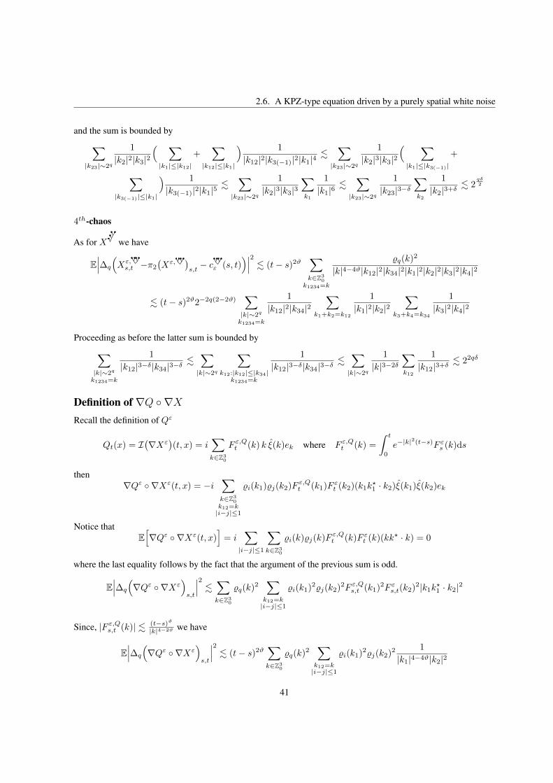
2.6. A KPZ-type equation driven by a purely spatial white noise
and the sum is bounded by|k23|∼2q
1
|k2|2|k3|2
|k1|≤|k12|
+
|k12|≤|k1|
1
|k12|2|k3(−1)|2|k1|4.
|k23|∼2q
1
|k2|3|k3|2
|k1|≤|k3(−1)|
+
|k3(−1)|≤|k1|
1
|k3(−1)|2|k1|5.
|k23|∼2q
1
|k2|3|k3|3k1
1
|k1|6.
|k23|∼2q
1
|k23|3−δk2
1
|k2|3+δ. 2
qδ2
4th-chaos
As for X we have
E∆q
Xε,s,t −π2
Xε,
s,t
− cε (s, t)2 . (t− s)2ϑ
k∈Z3
0k1234=k
ϱq(k)2
|k|4−4ϑ|k12|2|k34|2|k1|2|k2|2|k3|2|k4|2
. (t− s)2ϑ2−2q(2−2ϑ)
|k|∼2q
k1234=k
1
|k12|2|k34|2
k1+k2=k12
1
|k1|2|k2|2
k3+k4=k34
1
|k3|2|k4|2
Proceeding as before the latter sum is bounded by|k|∼2q
k1234=k
1
|k12|3−δ|k34|3−δ.
|k|∼2q
k12:|k12|≤|k34|
k1234=k
1
|k12|3−δ|k34|3−δ.
|k|∼2q
1
|k|3−2δ
k12
1
|k12|3+δ. 22qδ
Definition of ∇Q ∇X
Recall the definition of Qε
Qt(x) = I∇Xε
(t, x) = i
k∈Z3
0
F ε,Qt (k) k ξ(k)ek where F ε,Qt (k) =
t
0
e−|k|2(t−s)F εs (k)ds
then∇Qε ∇Xε(t, x) = −i
k∈Z3
0k12=k|i−j|≤1
ϱi(k1)ϱj(k2)Fε,Qt (k1)F
εt (k2)(k1k
⋆1 · k2)ξ(k1)ξ(k2)ek
Notice thatE∇Qε ∇Xε(t, x)
= i
|i−j|≤1
k∈Z3
0
ϱi(k)ϱj(k)Fε,Qt (k)F εt (k)(kk
⋆ · k) = 0
where the last equality follows by the fact that the argument of the previous sum is odd.
E∆q
∇Qε ∇Xε
s,t
2 .k∈Z3
0
ϱq(k)2k12=k|i−j|≤1
ϱi(k1)2ϱj(k2)
2F ε,Qs,t (k1)2F εs,t(k2)
2|k1k⋆1 · k2|2
Since, |F ε,Qs,t (k)| . (t−s)ϑ|k|4−2ϑ we have
E∆q
∇Qε ∇Xε
s,t
2 . (t− s)2ϑk∈Z3
0
ϱq(k)2k12=k|i−j|≤1
ϱi(k1)2ϱj(k2)
2 1
|k1|4−4ϑ|k2|2
41

Chapter 2. Multidimensional SDEs with Distributional Drift and Polymer Measure
and the sum is bounded byq.j
|i−j|≤1
|k|∼2q
k1:|k1|≤|k2|k12=k
+
k1:|k2|≤|k1|k12=k
ϱi(k1)
2ϱj(k2)2 1
|k1|4−4ϑ|k2|2.
q.j
|i−j|≤1
|k|∼2q
2−2j2−i(1−4ϑ−δ)
k1
1
|k1|3+δ+ 2−i(3−4ϑ−δ)
k2
1
|k2|3+δ. 23q
q.j
2−j(3−4ϑ−δ) . 2−2q(−2ϑ− δ2 )
and this concludes the proof.
2.6.3 The Renormalization Constants
We have seen in the previous section that the terms Xε,t − cε (t) and Xε,
t − cε (t) are convergent respectivelyin CTCρ+1 and CTC4ρ for all ρ < 1/2, where
cε (t) = EXε,t
, and cε (t) = E
Xε,t
Let us begin by analyzing cε (t). By Wick theorem, we have
E[∇Xε(t)∇Xε, (t)] = −2
k1,k2 =0;k1 =−k2
(k2 · k12)(k1 · k2)|k1|2|k2|4
(1− e−|k1|2s)|m(εk1)|2|m(εk2)|2
× t
0
ds
s
0
dσe−|k1|2(t−s)e−|k12|2(s−σ)(1− e−|k2|2s)(1− e−|k2|2σ)(1− e−|k1|2σ)
Now is not difficult to see that the latter t
0
s
0
dsdσe−|k1|2(t−s)e−|k12|2(s−σ)(1−e−|k1|2σ)(e−|k2|2s+e−|k2|σ+e−|k2|2(s+σ)) .t−1+ 3
2ν
|k12|2−ν |k2|2−ν |k1|2−ν
for ν > 0 small enough. Then, the previous sum can be bounded by
t3/2ν−1k1,k2
1
|k1|3−ν |k2|4−ν |k12|1−ν. t3/2ν−1
|k1|≤|k2|
+
|k2|≤|k1|
1
|k1|3−ν |k2|4−ν |k12|1−ν
t3/2ν−1(k1,k2
|k1|3+ν |k12|5−3ν +k1,k2
|k2|4−ν |k12|4−2ν) < +∞
for ν > 0 small enough. Then, to show convergence of E[∇X(t)∇X (t)], it remains to study the contributiongiven by the two following integrals t
0
ds
s
0
dσe−|k1|2(t−s)e−|k12|2(s−σ),
t
0
ds
s
0
dσe−|k1|2(t−s)e−|k12|2(s−σ)e−|k1|2σ.
A direct computation gives t
0
ds
s
0
dσe−|k1|2(t−s)e−|k12|2(s−σ) =1− e−|k1|2t
|k12|2|k1|2− 1
|k12|2
t
0
dse−|k1|2(t−s)e−|k12|2s (2.6.20)
42

2.6. A KPZ-type equation driven by a purely spatial white noise
and we observek1,k2
|(k2 · k12)(k1 · k2)||k1|2|k2|4|k12|2
(1− e−|k1|2t)
t
0
dse−|k1|2(t−s)e−|k12|2s .k1,k2
1
t1−ν |k1|3−ν |k2|2|k12|3−ν< +∞
where we have bounded the integral term as t0dse−|k1|2(t−s)e−|k12|2s . tν−1|k1|ν−1|k12|ν−1 for ν > 0 small
enough, and the convergence of the sum appearing at the right hand side is obtained as before. Now, let us focus onthe contribution to the sum given by the first summand at the right hand side of (2.6.20), i.e.
k1,k2 =0;k1 =−k2
(k2 · k12)(k1 · k2)|k1|4|k2|4|k12|2
(1− e−|k1|2s)2|m(εk1)|2|m(εk2)|2
Splitting this sum according to the following decomposition (1− e−|k21t)2 = 1+ e−|k1|2t(2 + e−|k1|2t) we are leadto the following terms
k1,k2,k12 =0
(k2 · k12)(k1 · k2)|k1|4|k2|4|k12|2
|m(εk1)|2|m(εk2)|2,
k1,k2,k12 =0
(k2 · k12)(k1 · k2)|k1|4|k2|4|k12|2
e−|k1|2t(2 + e−|k1|2t)|m(εk1)|2|m(εk2)|2
For the first, notice that
k1,k2,k12 =0
(k2 · k12)(k1 · k2)|k1|4|k2|4|k12|2
|m(εk1)|2|m(εk2)|2
=
k1,k2,k12 =0
k1 · k2|k1|4|k2|4
|m(εk1)|2|m(εk2)|2 −
k1,k2,k12 =0
(k1 · k12)(k1 · k2)|k1|4|k2|4|k12|2
|m(εk1)|2|m(εk2)|2
and thus
k1,k2,k12 =0
(k2 · k12)(k1 · k2)|k1|4|k2|4|k12|2
|m(εk1)|2|m(εk2)|2
=1
2
k1,k2,k12 =0
k1 · k2|k1|4|k2|4
|m(εk1)|2|m(εk2)|2 =1
2
k1 =0
|k1|−6|m(εk1)|4
where we have used that the function m is even, and by dominated convergence theorem we conclude that the righthand side converges to
k1 =0 |k1|−6 < +∞ as ε goes to zero. The second term instead
k1,k2,k12 =0
(k2 · k12)(k1 · k2)|k1|4|k2|4|k12|2
e−|k1|2t(2 + e−|k1|2t)|f(εk1)|2|f(εk2)|2
=
k1,k2,k12 =0
k1 · k2|k1|4|k2|4
|f(εk1)|2|f(εk2)|2e−|k1|2t(2 + e−|k1|2t)
−
k1,k2,k12 =0
(k1 · k12)(k1 · k2)|k1|4|k2|4|k12|2
e−|k1|2t(2 + e−|k1|2t)|f(εk1)|2|f(εk2)|2
43
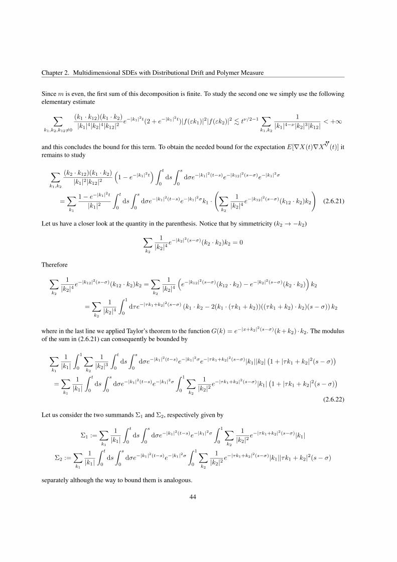
Chapter 2. Multidimensional SDEs with Distributional Drift and Polymer Measure
Since m is even, the first sum of this decomposition is finite. To study the second one we simply use the followingelementary estimate
k1,k2,k12 =0
(k1 · k12)(k1 · k2)|k1|4|k2|4|k12|2
e−|k1|2t(2 + e−|k1|2t)|f(εk1)|2|f(εk2)|2 . tν/2−1k1,k2
1
|k1|4−ν |k2|3|k12|< +∞
and this concludes the bound for this term. To obtain the needed bound for the expectation E[∇X(t)∇X (t)] itremains to study
k1,k2
(k2 · k12)(k1 · k2)|k1|2|k12|2
1− e−|k1|2t
t
0
ds
s
0
dσe−|k1|2(t−s)e−|k12|2(s−σ)e−|k1|2σ
=k1
1− e−|k1|2t
|k1|2
t
0
ds
s
0
dσe−|k1|2(t−s)e−|k1|2σk1 ·
k2
1
|k2|4e−|k12|2(s−σ)(k12 · k2)k2
(2.6.21)
Let us have a closer look at the quantity in the parenthesis. Notice that by simmetricity (k2 → −k2)
k2
1
|k2|4e−|k2|2(s−σ)(k2 · k2)k2 = 0
Therefore
k2
1
|k2|4e−|k12|2(s−σ)(k12 · k2)k2 =
k2
1
|k2|4e−|k12|2(s−σ)(k12 · k2)− e−|k2|2(s−σ)(k2 · k2)
k2
=k2
1
|k2|4
1
0
dτe−|τk1+k2|2(s−σ) (k1 · k2 − 2(k1 · (τk1 + k2))((τk1 + k2) · k2)(s− σ)) k2
where in the last line we applied Taylor’s theorem to the function G(k) = e−|x+k2|2(s−σ)(k+k2) ·k2. The modulusof the sum in (2.6.21) can consequently be bounded by
k1
1
|k1|
1
0
k2
1
|k2|3
t
0
ds
s
0
dσe−|k1|2(t−s)e−|k1|2σe−|τk1+k2|2(s−σ)|k1||k2|1 + |τk1 + k2|2(s− σ)
=k1
1
|k1|
t
0
ds
s
0
dσe−|k1|2(t−s)e−|k1|2σ 1
0
k2
1
|k2|2e−|τk1+k2|2(s−σ)|k1|
1 + |τk1 + k2|2(s− σ)
(2.6.22)
Let us consider the two summands Σ1 and Σ2, respectively given by
Σ1 :=k1
1
|k1|
t
0
ds
s
0
dσe−|k1|2(t−s)e−|k1|2σ 1
0
k2
1
|k2|2e−|τk1+k2|2(s−σ)|k1|
Σ2 :=k1
1
|k1|
t
0
ds
s
0
dσe−|k1|2(t−s)e−|k1|2σ 1
0
k2
1
|k2|2e−|τk1+k2|2(s−σ)|k1||τk1 + k2|2(s− σ)
separately although the way to bound them is analogous.
44

2.6. A KPZ-type equation driven by a purely spatial white noise
For Σ1, notice that for ε > 0 sufficiently small, one hask2
1
|k2|2e−|τk1+k2|2(s−σ)|k1| . |k1|
k2
1
|k2|2|τk1 + k2|2−2ε(s− σ)1−ε
.|k1|
(s− σ)1−ε
dy
|y|2|τk1 + y|2−2ε.
|k1|ε
τ1−ε(s− σ)1−ε
dy
|y|2| k1|k1| + y|2−2ε
where the integral is taken over a suitable subset of R3 where the integrand is well-defined. It is immediate to seethat the latter is bounded (for example by Cauchy-Schwartz).
Analogously, for Σ2, upon setting ε := ε2 > 0, we get
k2
1
|k2|2e−|τk1+k2|2(s−σ)|k1||τk1 + k2|2(s− σ) . |k1|
k2
1
|k2|2|τk1 + k2|2−ε(s− σ)1−ε
and the latter can be treated as before.At this point, given δ, γ > 0, (2.6.22) is bounded by
k1
1
|k1|
t
0
ds
s
0
dσe−|k1|2(t−s)e−|k1|2σ 1
0
|k1|ε
τ1−ε(s− σ)1−ε.k1
1
|k1|1−ε
t
0
ds
s
0
dσe−|k1|2(t−s)e−|k1|2σ
(s− σ)1−ε
.k1
1
|k1|1−ε
t
0
ds1
|k1|2−2γ(t− s)1−γ
s
0
dσ1
|k1|2−2δσ1−δ(s− σ)1−ε
.k1
1
|k1|5−2γ−2δ−ε
t
0
1
s1−δ−ε(t− s)δ.k1
t−1+γ+δ+ε
|k1|5−2γ−2δ−ε
and the last term is bounded provided that 5 − 2γ − 2δ − ε > 3 and −1 + γ + δ + ε > 0. Thereforesupt∈[0,T ] t
3/2ν−1|E[∇Xε(t)∇Xε, (t)]| is convergent and by dominated convergence we can conclude that the
constant cε does not diverge and can therefore be omitted.
We can now focus on the other constant. Applying Wick’s theorem in the same way we did for X and takinginto account the symmetricity of the sum in both k1, k2 and k3, k4, we obtain
cε (t) = 2
k1,k2∈Z30
F ε,t (0, k12, k12, k1, k2, k1, k2)|k12|2|k1 · k2|2
Now, we want to show that cε (t) = cε t+Rε(t), where cε is a diverging constant and Rε(t) is finite uniformlyin ε. By definition
cε (t) = 2k1,k2
2h=1
m(εkh)2
t
0
s
0
e−|k12|2(s−r)1− e−|k1|2r
1− e−|k2|2r
dr
2
ds|k12|2|k1 · k2|2
|k1|4|k2|4
For the inner integral we write s
0
e−|k12|2(s−r)1− e−|k1|2r
1− e−|k2|2r
dr = I1(s) + I2(s)
where
I1(s) : =1− e−|k12|2s
|k12|2I2(s) :=
3i=1
s
0
e−|k12|2(s−r)e−airdr
45
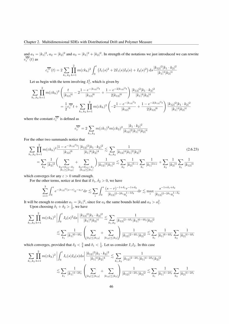
Chapter 2. Multidimensional SDEs with Distributional Drift and Polymer Measure
and a1 = |k1|2, a2 = |k2|2 and a3 = |k1|2 + |k2|2. In strength of the notations we just introduced we can rewritecε (t) as
cε (t) = 2k1,k2
2h=1
m(εkh)2
t
0
I1(s)
2 + 2I1(s)I2(s) + I2(s)2ds
|k12|2|k1 · k2|2
|k1|4|k2|4
Let us begin with the term involving I21 , which is given byk1,k2
2h=1
m(εkh)2
t
|k12|4− 2
1− e−|k12|2t
|k12|6+
1− e−2|k12|2t
2|k12|6
|k12|2|k1 · k2|2
|k1|4|k2|4
=1
2cε t+
k1,k2
2h=1
m(εkh)2
−2
1− e−|k12|2t
|k12|6+
1− e−2|k12|2t
2|k12|6
|k12|2|k1 · k2|2
|k1|4|k2|4
where the constant cε is defined as
cε = 2k1,k2
m(εk1)2m(εk2)
2 |k1 · k2|2
|k12|2|k1|4|k2|4
For the other two summands notice thatk1,k2
2h=1
m(εkh)2 |1− e−|k12|2t|
|k12|6|k12|2|k1 · k2|2
|k1|4|k2|4.k1,k2
1
|k12|4|k1|2|k2|2(2.6.23)
=k2
1
|k2|2
k2=k12−k1|k1|≤|k12|
+
k2=k12−k1|k12|≤|k1|
1
|k12|4|k1|2.k2
1
|k2|5−εk1
1
|k1|3+ε+k2
1
|k2|4k1
1
|k12|4
which converges for any ε > 0 small enough.For the other terms, notice at first that if δ1, δ2 > 0, we have
3i=1
s
0
e−|k12|2(s−r)e−airdr .i
s
0
(s− r)−1+δ1r−1+δ2
|k12|2−2δ1a1−1δ2i
dr . maxi
s−1+δ1+δ2
|k12|2−2δ1a1−δ2i
It will be enough to consider a1 = |k1|2, since for a2 the same bounds hold and a3 > a21.Upon choosing δ1 + δ2 >
12 , we have
k1,k2
2h=1
m(εkh)2
t
0
I2(s)2ds
|k12|2|k1 · k2|2|k1|4|k2|4.k1,k2
1
|k12|2−4δ1 |k1|6−4δ2 |k2|2
.k1
1
|k1|6−4δ2
|k2|≤|k12|
+
|k12|≤|k2|
1
|k12|2−4δ1 |k2|2.k1
1
|k1|6−4δ2
k2
1
|k2|4−4δ1
which converges, provided that δ2 < 34 and δ1 < 1
4 . Let us consider I1I2. In this case
k1,k2
2h=1
m(εkh)2
t
0
I1(s)I2(s)ds
|k12|2|k1 · k2|2|k1|4|k2|4.k1,k2
1
|k12|2−2δ1 |k1|4−2δ2 |k2|2
.k1
1
|k1|4−2δ2
|k2|≤|k12|
+
|k12|≤|k2|
1
|k12|2−2δ1 |k2|2.k1
1
|k1|4−2δ2
k2
1
|k2|4−2δ1
46
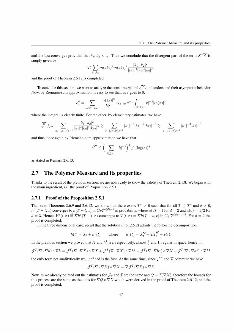
2.7. The Polymer Measure and its properties
and the last converges provided that δ1, δ2 < 12 . Then we conclude that the divergent part of the term Xε is
simply given by
2tk1,k2
m(εk1)2m(εk2)
2 |k1 · k2|2
|k12|2|k1|4|k2|4.
and the proof of Theorem 2.6.12 is completed.
To conclude this section, we want to analyze the constants cε and cε , and understand their asymptotic behavior.Now, by Riemann-sum approximation, it easy to see that, as ε goes to 0,
cε =
k∈Z3,k =0
|m(εk)|2
|k|2∼ε→0 ε
−1
|x|>1
|x|−2|m(x)|2
where the integral is clearly finite. For the other, by elementary estimates, we have
cε .m
|k1|,|k2|.ε−1
|k1 · k2|2
|k1|4|k2|2|k12|2.
|k1|,|k2|.ε−1
|k1|−2|k2|−2|k12|−2 .
|k1|,|k2|.ε−1
|k1|−3|k2|−3
and thus, once again by Riemann-sum approximation we have that
cε .
|k|.ε−1
|k|−32
. (log(ε))2
as stated in Remark 2.6.13.
2.7 The Polymer Measure and its propertiesThanks to the result of the previous section, we are now ready to show the validity of Theorem 2.1.8. We begin withthe main ingredient, i.e. the proof of Proposition 2.5.1.
2.7.1 Proof of the Proposition 2.5.1Thanks to Theorems 2.6.9 and 2.6.12, we know that there exists T ⋆ > 0 such that for all T ≤ T ⋆ and δ > 0,hε(T − t, x) converges to h(T − t, x) in CTCa(d)−δ in probability, where a(d) = 1 for d = 2 and a(d) = 1/2 ford = 3. Hence, V ε(t, x) def
= ∇hε(T − t, x) converges to V (t, x) = ∇h(T − t, x) in CTCa(d)−1−δ. For d = 2 theproof is completed.
In the three dimensional case, recall that the solution h to (2.5.2) admits the following decomposition
h(t) = Xt + h1(t) where h1(t) = Xt + 2Xt + v(t).
In the previous section we proved that X and h1 are, respectively, almost 12 and 1, regular in space, hence, in
J T (∇ ·∇h) ∇h = J T (∇ ·∇X) ∇X +J T (∇ ·∇X) ∇h1 +J T (∇ ·∇h1) ∇X +J T (∇ ·∇h1) ∇h1
the only term not analitytically well defined is the first. At the same time, since J T and ∇ commute we have
J T (∇ · ∇X) ∇X = ∇J T (∇X) ∇X
Now, as we already pointed out the estimates for JT and I are the same and Q = I(∇X), therefore the bounds forthis process are the same as the ones for ∇Q ∇X which were derived in the proof of Theorem 2.6.12, and theproof is completed.
47

Chapter 2. Multidimensional SDEs with Distributional Drift and Polymer Measure
2.7.2 Global existence, Parabolic Anderson equation and Feynman-Kac representationIn this section we want to show the global existence of the polymer measure. By the construction carried out inSection 2.5, the result immediately follows if we are able to prove that the solution to the KPZ-type equation (2.5.3)does not explode in finite time. So, let once again hε satisfy
∂thε =
1
2∆hε +
1
2|∇hε|2 + ξε − cε, h(0, x) = 0.
Now, we know that there exists a time T ⋆ > 0 such that hε converges to a function h in CTCa(d)−δ in probability,where a(d) = 1 for d = 2 and a(d) = 1/2 for d = 3, independently of the mollifier, for all T ≤ T ⋆. Moreoverin [GIP15a] and [HL15b], the authors proved global well-posedness for the parabolic Anderson equation indimension d = 2 and 3, respectively, namely they showed that there exists a constant bε for which if vε denotes thesolution of
∂tvε =
1
2∆vε + vεξε − bεv
ε, vε(0, x) = 1 (2.7.1)
then for all T > 0, vε converges in CTCa(d)−δ (in probability) to a function v independently of the approximationof the noise, and the constant bε can be chosen to be cε. We need to take into account the following two facts
1. By Feynman-Kac formula, vε can be written as
vε(t, x) = Exe t0(ξε(Bs)−cε)ds
2. The Cole-Hopf transform of hε solves (2.7.1), i.e. vε(t, x) = eh
ε(t,x) for all t ≤ T ⋆ and x ∈ T2. Therefore,taking the limit as ε tends to 0 we have v(t, x) = eh(t,x) > 0 for t ≤ T ⋆.
Now, the point is that for all t ≤ T ⋆, the Markov property implies
vε(t+ T ⋆, x) = EWx
e T⋆
0(ξε(Bs)−cε)dsvε(t, BT⋆)
= vε(T ⋆, x)EQε
x,T⋆[vε(t, BT⋆)]
thus, since Qεx,T converges weakly to a probability measure Qx,T⋆ and ∥vε − v∥CTL∞ → 0 we get immediately, bytaking the limit as ε→ 0, that
v(T ⋆ + t, x) = v(T ⋆, x)EQx,T⋆ [v(t, BT⋆)] > 0
for all t ≤ T ⋆ which implies that v(t, x) > 0 for all t ≤ 2T ⋆ and x ∈ T2. Iterating the same argument, we get thatv(t, x) > 0 for all t ≥ 0 and all x. At this point, it is not difficult to see that we can extend hε and h to the wholehalf-line [0,+∞) by setting hε(t) = log(vε(t)) and h(t) = log(v(t)) for all t ≥ 0. Therefore, it is immediate toverify that the h constructed in this way is a global in time solution of the equation (2.5.3).
2.7.3 Singularity with respect to the Wiener measureWe will give the proof in the case of dimension 3 since an analogous, but simpler argument, holds for d = 2.
In order to verify that the Polymer measure QT,x is singular with respect to the Wiener measure Wx, we willbegin by showing that the sequence of densities dQNT,x/dW (we are taking ε to be 1/N ) admits a subsequenceconverging to 0 W-a.s. At first notice that, by Feynman-Kac formula, for all T ≤ T ⋆ we have
ehN (T,x) = e−cNTEWx
e T0ξN (ωs)ds
= ZTNe
−cNT
where hN is the solution to (2.5.2) driven by the mollified noise ξN , cNdef= cN + cN and cN , cN are the diverging
constants introduced in Theorem 2.6.12. Now, let YN be the random variable given by
YN (ω) := (ZTN )−1e T0ξN (ωs)ds
48
2.7. The Polymer Measure and its properties
and δ < 1 be fixed. Thanks to the last part of the above mentioned theorem, we immediately see that
EW[(YN )δ] = (ZTN )−δEW
e T0δξN (ωs)ds
= e(−cNδ(1−δ)+δ
4cN )T ehNδ (T,x)−hN (T,x) (2.7.2)
where, this time, hNδ is the solution to the KPZ-type equation (2.5.2) driven by δξN and ξN is the same as before.Since, by Remark 2.6.13 as N → ∞, cN ∼ N while cN = O((logN)2), we have
limN→+∞
cNδ(1− δ)− (δ4 − δ)cN = limNcNδ(1− δ) = +∞
it follows that there exists a subsequence (denoted once again as the argument of the limit at the left hand side ofthe previous) for which the the first exponential at right hand side of (2.7.2) is summable. Moreover, thanks toTheorem 2.6.9 the second exponential converges, as N → ∞ to exp
hδ(T, x)− h(T, x)
. Therefore
N
EW(Y N )δ
.N
e(−cNδ(1−δ)+(δ4−δ)cN )T < +∞
which in particular implies that, if ArN = YN < r, then W(lim supN ArN ) = 1.
The point is to prove that instead Q(lim supN ArN ) = 0. By Portemanteau theorem we have
Q(ArN ) ≤ lim infL→+∞
QL(ArN )
so we need to suitably bound QL(ArN ). Let us notice that
QL(ArN ) = EWYL1Ar
N
. rδ(ZL)
−1(ZN )δEW
e T0ξL(ωs)−δξN (ωs)ds
Denoting by cL the diverging constant associated to hL and upon using once again the inequality (ZL)
−1(ZN )δ .eT (δcN−cL), we get
QL(ArN ) . eT (δcN−cL)EW
e T0ξL(ωs)−δξN (ωs)ds
Let hN,Lδ be the solution of the equation
∂thN,Lδ =
1
2∆hN,Lδ +
1
2|∇hN,Lδ |2 + ξL − δξN − (cN,L + cN,L), hN,Lδ (0, x) = 0.
and we apply again Feynmann-Kac formula, so that
EW
e T0ξL(ωs)−δξN (ωs)ds
= eh
N,Lδ (T,x)+T (cN,L+cN,L)
Now we claim that, if we take the constants cN,L and cN,L as
cN,L = cL + (δ2 − 2δ)cN , and cN,L = cL + δ(δ3 − 4δ2 + 5δ2 − 4)cN (2.7.3)
then there exists a function h such that, for all T ≤ T ⋆
limN→∞
limL→∞
hN,Lδ (T, x) = h(T, x) (2.7.4)
Assuming (2.7.4) holds true we are done. Indeed,
Q(ArN ) . lim inf QL(ArN ) . e(−cNδ(1−δ)+δ(δ3−4δ2+5δ2−3)cN )T eh(T,x) . e−cNδ(1−δ)T/2
49
Chapter 2. Multidimensional SDEs with Distributional Drift and Polymer Measure
valid for N large enough, where the last passages are due to the asymptotic behaviour of the two constants. At thispoint, Borel-Cantelli lemma guarantess that Q(lim supN A
rN ) = 0, which in turn implies that Q is singular with
respect to the Wiener measure.
The only missing ingredient is the proof of the claim (2.7.4). Recall that
hN,L = ScKPZξL − δξN , cN,L + cN,L
= SrKPZ
XξL − δξN , cN,L, cN,L
where the two maps ScKPZ and SrKPZ were introduced in Theorem 2.6.9. To ensure the convergence of hN,L itsuffices to exploit the continuity of the map SrKPZ and show that there exists a choice of cN,L, cN,L for which the
sequence XξL − δξN , cN,L, cN,L
converges in X ϱ.
Now, the first two components of XξL − δξN , cN,L, cN,L
are given by
XN,L = I(ξL − δξN ), XN,L, = I(|∇XN,L|2)
and, expanding the product at the second term we get
XN,L, = XL, + δ2XN, − 2δI(∇XL∇XN )
where we have set XL, = I(|∇XL|2). Since the first two summands at the right hand side were already treated inthe Theorem 2.6.12, we will only focus one the last one. We can assume, without loss of generality, that L > N + 5(remember that we want to take the limit in L before the one in N ). Of course the only ill-defined part of this termin the limit is given by the resonant term I(∇XL ∇XN ). Observe that
I(∇XL ∇XN ) = I(∇XN+5 ∇XN )
since F (XL −XN+5) and F (XN ) have disjoint support. Moreover the same argument used in Theorem 2.6.12allows to show that the limit of the sequence I(∇XN+5∇XN − cN ) exists in CκC2ϱ for all κ > 0 and ϱ < 1/2.Choosing cN,L = cL + (δ2 − 2δ)cN , the term XN,L, − I(cN,L) converges, as L tends to ∞, to
X + δ2(XN, − I(cN )) + 2δI(∇(X −XN+5) ≺ ∇XN +∇(X −XN+5) ≻ ∇XN +∇XN+5∇XN − cN )
in CTC2ϱ, and the latter converges in the N → ∞-limit in the space CTC2ϱ.
At this point we have proved the convergence of the first two terms of X(ξL − δξN , cN,L, cN,L, cN,L) and thisis enough to conclude the proof in the two dimensional case thanks to Remark 2.6.11.
By repeating essentially the same argument exploited in the proof of Theorem 2.6.12, we see that there exists aconstant cN,L auch that X(ξL − δξN , cN,L, cN,L) converges as L goes to the infinity to some element XN ∈ X ρ
for all ρ < 1/2. For the same reason as before, we can take the limit in N . The conclusion now follows by thecontinuity of the map SrKPZ . Indeed, hN,L converges in the space CTCα and of course this in particular impliesthat
limN
limLhN,L(t, x) = h(t, x)
where h = SrKPZlimN limLX(ξL− δξN , cN,L, cN,L)
and the proof of the claim (and therefore of the theorem)
is completed.
50
Chapter 3
Malliavin Calculus for RegularityStructures: the case of gPAM
The content of this chapter is based on [CFG15] and aims at concretizing what briefly outlined in Section 1.3 of theIntroduction.
The goal of the work presented here is, in general, to introduce Malliavin Calculus techniques in the context ofRegularity Structures, and in particular, to prove that the solution to gPAM, when evaluated at a space-time point,admits a density with respect to the Lebesgue measure. Recall that the generalized Parabolic Anderson Equation(gPAM), is formally given by
(∂t −∆)u = g(u)ξ, u(0, ·) = u0(·). (3.0.1)
for t ≥ 0, the space variable belonging to the two-dimensional torus T2, g sufficiently smooth, spatial white noiseξ = ξ(x, ω) and fixed initial data u0. As a first step in our analysis, we want to understand how the solution to (3.0.1)behaves when we perturb the noise in Cameron-Martin directions. More precisely, let H be the Cameron-Martinspace associated to the white noise (i.e. H = L2(T2)), then, for h ∈ H, we will consider the solution uh of theperturbed equation
(∂t −∆)uh = g(uh)(ξ + h), u(0, ·) = u0(·). (3.0.2)
in which the initial condition is the same as before (i.e. u0), but the noise has been replaced by its translated version(i.e. ξ + h). Now, if we formally set vh def
= ∂∂εu
εh|ε=0, then vh should satisfies the tangent equation
(∂t −∆)vh = g(u)h+ vhg′(u)ξ, vh0 (·) = 0. (3.0.3)
which, we have to prove, corresponds to the Malliavin derivative of u evaluated at h, i.e. vh = ⟨Du, h⟩H. At thispoint, if all this could be consistently done, it would remain to show that such a Malliavin derivative is non-degenrate,to conclude that u(t, x;ω) admits a density with respect to the Lebesgue measure.
The rest of the chapter is organized as follows. Sections 3.1 and 3.2 are somewhat introductory. In the first, webriefly recall the tools of Malliavin Calculus we will need. In the second, we will initially build a common ground onwhich to define the previous equations, constructing a regularity structure that contains all the processes that appearin the description of u, uh and vh as well as the ones needed to solve (3.0.1), (3.0.2) and (3.0.3). Then we willreview the main ingredients of the theory of Regularity Structures and the solution theory for the aforementionedequations. In Section 3.3, we prove that vh is indeed the Malliavin derivative of u evaluated at h and list itsmain properties. Finally, in Section 3.4, after providing the strong maximum principle a la Mueller announced inthe Introduction, we show that u admits a density with respect to the Lebesgue measure conditioned to non-exploding.
51
Chapter 3. Malliavin Calculus for Regularity Structures: the case of gPAM
Function Spaces and Notations. We collect here some definitions and notations we will use throughout. LetS ′(Rd) be the space of Schwartz distributions, α < 0 and r := −⌊α⌋. Then, we say that f ∈ S ′(Rd) belongs toCα(Rd) (locally) if it belongs to the dual of Cr and for every compact set D ⊂ Rd
∥f∥α,D := supz∈D
supϕ∈Br
1
supλ∈(0,1]
λ−α|⟨f, ϕλz ⟩| <∞
where Br1 is the space of Cr functions compactly supported in the unit ball whose Cr-norm is less or equal to 1 andϕλx is the rescaled version of ϕ ∈ Br1 centered at x ∈ Rd, i.e. ϕλx(y) = λ−dϕ(λ−1(y − x)).
Since we will be working on parabolic equations, we also introduce the parabolic version of Cα on Rd+1, whichis obtained by simply replacing the rescaled function in the following way
ϕλz (w) := λ−2−dϕ(λ−2(t− s), λ−1(x− y)). (3.0.4)
where z = (t, x) and w = (s, y) ∈ R1+d.To treat the case of α > 0, we need the parabolic norm on R1+d, which, abusing notation, is given by
|z − w| :=|t− s|+ |x− y|
for z = (t, x) and w = (s, y) ∈ R1+d. Now, for α ∈ (0, 1) and η ∈ R, we define the weighted space of (locally)Holder continuous functions Cα,η(R+ × Rd) as the set of those f such that for any compact D ⊂ (0,∞)× Rd
∥f∥Cα,η := supz=(t,x)∈D
t−η∧02 |f(z)|+ sup
z=(t,x),w=(s,y)∈D|z−w|≤(t∧s)
12
(t ∧ s)α−η
2 ∨0 |f(z)− f(w)||z − w|α
<∞ (3.0.5)
where, again, the generic points z, w ∈ R+ × R2 have to be understood as z = (t, x) and (s, y).
3.1 Malliavin Calculus in a nutshellIn this section, we simply want to recall tools and notations of Malliavin calculus that we will need in the rest of thechapter (for a thourogh introduction see for example [Nua06]).
Let (Ω,H,P) be an abstract Wiener space, i.e. Ω is a separable Banach space, P a zero-mean Gaussianprobability measure with full support on Ω and H the associated Cameron-Martin space, and F the completion ofthe Borel σ-algebra on Ω with respect to P. We know that each element y ∈ Ω⋆ defines a gaussian random variablethat can be denoted by W (y). Then, W can be extended to H and is an isonormal gaussian process on (Ω,F ,P)according to Definition 1.1.1 in [Nua06].
Now, we say that a random variable F on Ω is smooth, if it can be written as F = f(W (h1), . . . ,W (hn)),where h1, . . . , hn ∈ H and f is an infinitely continuously differentiable function such that f and all its partialderivatives have (at most) polynomial growth. For a smooth random variable, we can define its Malliavin derivativeas (Definition 1.2.1 in [Nua06])
DF :=ni=1
∂if(W (h1), . . . ,W (hn))hi
and, since D is closable from Lp(Ω) to Lp(Ω;H) for all p ≥ 1, we can set D1,p to be the closure of the set ofsmooth random variables under the norm
∥F∥1,p := (E[|F |p] + E[∥DF∥pH])1p
where ∥ · ∥H is the norm on H. Thanks to the local properties of the Derivative operator, we can now localize thedefinition of D1,p. A random variable F ∈ D1,p
loc if there exists a sequence (Ωn, Fn)n≥1 ⊂ F × D1,p such thatΩn ↑ Ω, and Fn = F almost surely on Ωn.
52
3.2. The framework
We aim at proving that the solution to (3.0.1) admits a density with respect to the Lebesgue measure, a classicaltool in this context is provided by a criterion due to Bouleau and Hirsch [BH86] that we now recall (the formulationbelow is borrowed by [Nua06] Theorems 2.1.2 and 2.1.3)
Theorem 3.1.1. Let F be a real-valued random variable on (Ω,F ,P). If F ∈ D1,ploc for p ≥ 1, then F , conditioned
by the set ∥DF∥H > 0, is absolutely continuous with respect to the Lebesgue measure.
The analysis of the above mentioned equation we will perform in the upcoming sections, is pathwise, hence weneed a notion of differentiability better adapted to this construction. Moreover we lack a global well-posednessresult for (3.0.1) in the sense that we cannot prevent a priori an explosion of the L∞ norm of its solution, hence thedefinition of H-differentiability given by Definition 4.1.1 in [Nua06] is too strong in our context and we insteadresolve to use Definition 3.3.1 (c) in [UZ00].
Definition 3.1.2 (Local H-Differentiability). Let (Ω,H,P) be an abstract Wiener space. We will say that arandom variable F is locally H-differentiable if there exists an almost surely positive random variable q such thath →→ F (ω + h) is continuously differentiable on h ∈ H : ∥h∥H < q(ω). The set of full measure Q = q > 0will be called the set of differentiability of F . Finally we will indicate by C1
H−loc the set of all locally H-differentiablefunctions.
Remark 3.1.3. Of course, if for F ∈ C1H−loc, q can be taken to be equal to +∞ almost surely, then F ∈ C1
Haccording to Definition 4.1.1 in [Nua06].
As pointed out before, the definition above represents the local version of the usual notion of H-differentiability.We need to verify that it is not too weak, in the sense that the Bouleau and Hirsch’s criterion (Theorem 3.1.1) canstill be applied. This is indeed the case as we will see in the following proposition, whose proof is completelyanalogous to Proposition 4.1.3 in [Nua06] (or to the one of Proposition 3.4.1 in [UZ00]) and therefore we limitourselves to indicate the differences.
Proposition 3.1.4. We have C1H−loc ⊂ D1,2
loc .
Proof. Let F ∈ C1H−loc and q the strictly positive random variable introduced in Definition 3.1.2. For n ∈ N, let
An ⊂ Ω be given by
An =
ω ∈ Ω : q(ω) ≥ 4
n, sup
∥h∥H<2n
|F (ω + h)| ≤ n, sup∥h∥H<
2n
∥DF (ω + h)∥H ≤ n
then, since F is locally H-differentiable, Ω =
nAn a.s.. Moreover, thanks to Corollary 8.3.10 in [Str10], for all
n ∈ N there exists a σ-compact set Gn ⊂ An such that P(Gn) = P(An). For A ∈ F , set
ρA(ω) := inf∥h∥H : ω + h ∈ A
and let φ be a non-negative, C∞(R) compactly supported function such that |φ(t)| ≤ 1, |φ′(t)| ≤ 4 for all t andφ(t) = 1 for |t| ≤ 1
3 and 0 for |t| > 23 .
Then, it is easy to show (exploiting essentially the properties of ρ, see pg. 230 in [Nua06] or Lemma 3.4.2in [UZ00], and Exercise 1.2.9 in [Nua06]) that Fn := φ(nρGn)F is the localizing sequence required in the definitionof D1,2
loc .
3.2 The framework
3.2.1 The Regularity Structure for gPAMRecall that a regularity structure is a triplet T = (A, T,G) in which, A ⊂ R is a locally finite bounded from belowset of homogeneities, T =
α∈A Tα, the model space, is a graded vector space, and G, the structure group, is a set
of linear transformations on T such that for every Γ ∈ G and τ ∈ Tα, Γτ − τ ∈
β<α Tβ .
53
Chapter 3. Malliavin Calculus for Regularity Structures: the case of gPAM
The construction of the regularity structure Tg = (Ag, Tg, Gg) needed to solve (3.0.1) was already carried outin several papers (see [Hai14, HP14, HL15b]), hence we limit ourselves to recalling its main ingredients. At first,one defines two sets, U , containing all the symbols appearing in the description of the solution to (gPAM), andW , containing the ones needed to make sense of the right-hand side of the equation, as the smallest collectionssuch that 1, Xk
i , for k ∈ N and i = 1, 2, belong to U and, whenever τ ∈ U then τΞ ∈ W , while for every τ ∈ W ,I(τ) ∈ U . In the previous, Xk are the symbols corresponding to the polynomials, Ξ to the noise and I is theabstract integration map. The model space T is then given by the set of finite linear combinations of elements inW ∪ U and can be nicely decomposed as the direct sum of ⟨W⟩ and ⟨U⟩.
To each of the symbols so constructed we can then associate a homogeneity, |1| = 0, |Xj | = 1, |Ξ| = αmin,where
αmin = −1− κ
for κ > 0 small enough, and then recursively, for every τ , τ
|τ τ | = |τ |+ |τ |, |I(τ)| = |τ |+ 2
so that the graded structure on T is simply obtained by defining Tβ as the set of finite linear combinations of thosesymbols in T with homogeneity equal to β.
It turns out that, to solve the equation (3.0.1), we will not need the whole model space as previously constructedbut it will be sufficient to consider those elements in U and W with homogeneity respectively less than a fixedthreshold γ, slightly greater than −αmin, and γ + αmin. We will indicate the union of this restricted sets of symbolsby F . Hence, the model space we will use from now on is
Tg = ⟨F⟩ = TW ⊕ TU := ⟨Ξ, I(Ξ)Ξ, XiΞ : i = 1, 2⟩ ⊕ ⟨1, I(Ξ), Xi : i = 1, 2⟩
and its associated set of homogeneities is
Ag = αmin, 2αmin + 2, αmin + 1, 0, αmin + 2, 1.
In order to describe the structure group we first introduce the vector space T+g , whose basis vectors are symbols
of the formXk
Jl(τl), τl ∈ Tg
where k ∈ N2 and factors Jl(τl) are omitted whenever |τl|+ 2− |l| ≤ 0. Analogously to what done before, we canassign to each of these symbols a homogeneity, |1| = 0, |Xi| = 0 and then recursively, for τ ∈ Tg and τ1, τ2 ∈ T+
g ,|Jl(τ)| = |τ |+ 2− |l| and |τ1τ2| = |τ1|+ |τ2|. We then define the linear map ∆ : Tg → Tg ⊗ T+
g via
∆1 = 1⊗ 1, ∆Xi = Xi ⊗ 1 + 1⊗Xi, ∆Ξ = Ξ⊗ 1
and then recursively, for τ , τ ∈ Tg
∆τ τ = (∆τ)(∆τ), ∆I(τ) = (I ⊗ Id)∆τ +l,k
1
k! l!Xk ⊗X lJk+l(τ) (3.2.1)
where Id is the identity and the sum runs over finitely many k, l since Jk+l(τ) = 0 if |τl|+ 2− |l| − |k| ≤ 0. Now,let G+ be the family of linear functionals f : T+
g → R, such that, for any τ , τ ∈ T+g , f(τ τ) = f(τ)f(τ), the
structure group Gg will be then composed by the maps Γf given by
Γfτ = (Id ⊗ f)∆τ (3.2.2)
According to Proposition 8.21 in [Hai14], Gg is a group and, thanks to Theorem 8.24, it satisfies the structure grouprelation Γfτ − τ ∈
β<α Tβ for every τ ∈ Tα. If we now specialize to the case at study, it is immediate to verify
54
3.2. The framework
that, for a given f ∈ G+, the action of Γf on the elements of Tg , can be represented as the matrix
Γf =
1 f(J (Ξ)) f(X1) f(X2)0 1 0 00 0 1 00 0 0 1
OO 1 f(J (Ξ)) f(X1) f(X2)
0 1 0 00 0 1 00 0 0 1
(3.2.3)
Thanks to the previous, the group structure of Gg becomes explicit. More specifically, for f1, f2 ∈ G+, one candirectly show that Γf1Γf2 = Γf1+f2 , Γ−1
f1= Γ−f1 and that the identity matrix is the identity of the group. Moreover,
TW and TU are invariant under the action of the structure group and therefore, according to Definition 2.5 in [Hai14],are sectors of T of regularity αmin and 0, respectively.
3.2.2 Enlarging Tg
In order to be able to formulate (3.0.2) at the abstract level we need to suitably enlarge the regularity structure justconstructed without altering its characterizing features. To do so, we will add a symbol H that will play the samealgebraic role as the symbol for the noise, Ξ, but whose realization through the model will possess further propertiesthat we will specify later on. Let us then define two sets UH and WH such that U ⊂ UH , W ⊂ WH and, as before,
τ ∈ UH ⇐⇒ τΞ, τH ∈ WH τ ∈ WH =⇒ I(τ) ∈ UH
The vector space TH will be simply given by the set of finite linear combinations of elements in UH ∪WH and, alsoin this case, it can be conveniently decomposed as the direct sum of ⟨WH⟩ and ⟨UH⟩. We can assign a homogeneityto each element following the same rules prescribed in the previous section, imposing though |H| = αmin.
Once again, we define FH as the set of symbols in WH and UH of homogeneity less than γ + αmin and γ,respectively, and set
THg = ⟨FH⟩ = TWH ⊕ TUH :=
⟨Ξ, H, I(Ξ)Ξ, I(Ξ)H, I(H)Ξ, I(H)H,XiΞ, XiH : i = 1, 2⟩ ⊕ ⟨1, I(Ξ), I(H), Xi : i = 1, 2⟩
whose associated set of homogeneities is the same as before, i.e. AHg = αmin, 2αmin+2, αmin+1, 0, αmin+2, 1.Concerning the definition of the structure group, we impose the symbol H (and all the ones containing it) to
behave, at the algebraic level, analogously to Ξ. More specifically, let (THg )+ be the vector space, whose basisvectors are
Xk
Jl(τl) : τl ∈ THg and |τl|+ 2− |l| > 0
and assign to each of its elements a homogeneity according to the same rules as for the elements in T+g . Then, we
extend ∆ to a map ∆H : THg → THg ⊗ (THg )+ in such a way that
∆HH = H ⊗ 1, ∆Hτ = ∆τ for all τ ∈ Tg
and the relations in (3.2.1) still hold. Finally, defining GH+ as the set of linear functionals f : (THg )+ → R such thatf(τ τ) = f(τ)f(τ) for all τ , τ ∈ (THg )+, the structure group will be given by those Γf , f ∈ GH+ , acting on THg asin (3.2.2) but with ∆ substituted by ∆H .
55

Chapter 3. Malliavin Calculus for Regularity Structures: the case of gPAM
At last, we notice that, when restricted to THg , the action of Γf can be expressed as
Γf =
1 0 f(J (Ξ)) 0 f(J (H)) 0 f(X1) 0 f(X2) 00 1 0 f(J (Ξ)) 0 f(J (H)) 0 f(X1) 0 f(X2)0 0 1 0 0 0 0 0 0 00 0 0 1 0 0 0 0 0 00 0 0 0 1 0 0 0 0 00 0 0 0 0 1 0 0 0 00 0 0 0 0 0 1 0 0 00 0 0 0 0 0 0 1 0 00 0 0 0 0 0 0 0 1 00 0 0 0 0 0 0 0 0 1
O
O 1 f(J (Ξ)) f(J (H)) f(X1) f(X2)0 1 0 0 00 0 1 0 00 0 0 1 00 0 0 0 1
(3.2.4)
Once more, the same conclusions established before hold in this case as well, i.e. the group structure of GHg isexplicit and the subspaces TWH and TUH are sectors of regularity αmin and 0, respectively.
Finally, we point out that, by construction, Tg ⊂ T Hg in the sense of Section 2.1 of [Hai14], where T H
g =
(AHg , THg , G
Hg ).
Remark 3.2.1. The construction just carried out is a straight-forward generalization of the one in Section 8.1in [Hai14] and corresponds to the case in which we have more than one symbol for the noise (see for example [ZZ15],where this is done in the context of the Navier-Stokes equation). Nevertheless, we underline once more that thesymbol H has a completely different meaning and has been introduced at the sole purpose of keeping track of thetranslation of the noise at the abstract level. In particular, the homogeneity of these symbols is somewhat artificialas we will see in the following section.
3.2.3 Admissible ModelsThe objects constructed in the previous section are, for the moment, pure symbols to which we want to associatea suitable family of distributions. To this aim, Hairer introduces the notion of model for a general regularitystructure T = (A, T,G), i.e. a pair of maps Z = (Π,Γ), where Π : R3 → L(T,S ′(R3)) (with L(X,Y ) the setof linear functionals from X to Y ) and Γ : R3 × R3 → G, such that, for every x, y, z ∈ R3, ΠxΓxy = Πy andΓxyΓyz = Γxz . Moreover, for every γ > 0 and compact set D there exists a constant Cγ,D such that
|⟨Πxτ, ϕλx⟩| ≤ Cγ,D∥τ∥λ|τ | and ∥Γxyτ∥m ≤ Cγ,D∥τ∥|x− y||τ |−m (3.2.5)
uniformly over symbols τ ∈ T with homogeneity strictly smaller than γ, ϕ ∈ Br1 for r the smallest integer strictlygreater that minA, x, y in a compact and m ∈ A less than |τ | (here and later, the rescaling of ϕ has to be understoodin parabolic sense, see (3.0.4), unless otherwise stated). We endow the family of models with the system ofseminorms |||Z|||γ;D := ∥Π∥γ;D + ∥Γ∥γ;D defined as the smallest constant Cγ,D such that the bounds in (3.2.5)hold.
Among the set of models, we need to identify a suitable subset embracing the main constituents of our equations.To begin with, following Section 5 in [Hai14], we rewrite the heat kernel K in spatial dimension d = 2 as the sumof two terms, a “singular” part K (represented in our regularity structure by the symbol I) and a smooth remainderR (that, being smooth, can simply be “lifted” through the polynomials), in such a way that
1. K is compactly supported in |x|2 + t ≤ 1, is symmetric in the spatial variable x and is 0 for t ≤ 0,
2. for (t, x) such that |x|2 + t < 12 and t > 0, one has
K(t, x) =1
|4πt|e−
|x|24t
and it is smooth on |x|2 + t ≥ 14,
56

3.2. The framework
3. K annihilates every polynomial of parabolic degree less than 3.
Remark 3.2.2. We are allowed to split the heat kernel thanks to Lemma 5.5 in [Hai14]. Indeed, it precisely satisfiesthe scaling condition there required.
At this point all the elements are in place and we can define the family of so called admissible models for eitherof the regularity structures constructed before.
Definition 3.2.3. A model (Π,Γ) =: Z on Tg (resp. T Hg ) is said to be admissible if, for every x, y ∈ R3, the
following conditions hold
1. Πx1(y) = 1 and for every multiindex k ∈ N2 and τ ∈ W (resp. WH ) such that τXki ∈ Tg (resp. THg )
ΠxτXki (·) = (· − xi)
kΠxτ (3.2.6a)
and for every τ ∈ W (resp. WH ) such that I(τ) ∈ Tg (resp. THg ),
ΠxI(τ)(y) = ⟨Πxτ ,K(y − ·)⟩+
|l|<|τ |+2
(y − x)l
l!fx(Jl(τ)) (3.2.6b)
where fx is an element in G+ (resp. GH+ ), characterized by1
fx(Xi) = −xi (3.2.7)
and, again for every τ ∈ W (resp. WH ) such that I(τ) ∈ Tg (resp. THg ),
fx(Jl(τ)) = −⟨Πxτ,D(l)K(x− ·)⟩, |l| < |τ |+ 2 (3.2.8)
2. The map Γ is given via the relationΓxy = (Γfx)
−1Γfy . (3.2.9)
The existence of such admissible models is non-trivial. Nevertheless, it turns out that it is always possible to lifta smooth function (say a mollification of the noise) ξε to an admissible model imposing (3.2.6), (3.2.9), in additionto
ΠεxΞ(y) = ξε(y) and Πεxτ τ(y) = Πεxτ(y)Πεxτ(y) (3.2.10)
as it was shown in [Hai14], Proposition 8.27. We will refer to such a model as the canonical model. Moreover, forT = Tg or THg (and similar for T ), we say that an admissible model is smooth if Π : R3 → L(T, C∞(R3)) is asmooth function (cf. [HW15]; note that every canonical model is smooth). We then define M (T ), a separablespace of admissible models, as the closure of the set of smooth admissible models under the family of semidistances
|||Π− Π|||D := supx∈D
supϕ∈Br
1
supλ∈(0,1]
supτ∈T
λ−|τ ||⟨Πxτ − Πxτ, ϕλx⟩| (3.2.11)
where D is a compact subset of R3 and r := −⌊αmin⌋.
Remark 3.2.4. Let (Π,Γ) be an admissible model. The algebraic properties of the model and (3.2.9) in the previousdefinition convey an extremely important fact, i.e. the quantity Πx(Γfx)
−1 is independent of the base point x, or inother words, for every x, y we have
Πx(Γfx)−1 = Πy(Γfy )
−1 (3.2.12)
The reason why we are stating it explicitly is that a partial inverse hold. Indeed, if for a pair of maps (Π,Γ), (3.2.9)and (3.2.12) hold, then the algebraic relations characterizing a model are immediately satisfied, and this will becrucial in what follows.
1Due to multiplicativity of such elements, this determines fx on T+g (resp. TH
g+).
57
Chapter 3. Malliavin Calculus for Regularity Structures: the case of gPAM
Remark 3.2.5. It might appear weird that in the definition of the semidistance (3.2.11) there is no reference to themap Γ. As already pointed out in Remark 2.4 of [HW15] and Remark 3.5 of [HP14], if (Π,Γ) is a pair of maps forwhich the first analytical bound in (3.2.5) and the equalities (3.2.6) and (3.2.9) hold then also the second analyticalbound in (3.2.5) is automatically satisfied thanks to Theorem 5.14 in [Hai14]. For the reader’s convenience, we givea short and self-contained proof of this in our setting in Appendix 3.5.2.
Remark 3.2.6. We point out that as a consequence of Definition 3.2.3, the relation (3.2.2) and the previous remark,for an admissible model (Π,Γ), the action of the map Γ is fully determined by the map
f : x →→ fx
introduced in Definition 3.2.3 above, hence we will denote an admissible model either by (Π,Γ) or by (Π, f)without further notice.
Remark 3.2.7. As a final remark, we will consider only models adapted to the action of a subgroup of thetranslations, according to Definition 3.33 in [Hai14]. More specifically, this means that, if e1 and e2 are thecanonical basis vectors on R2 and Ti : R3 → R3 is given by Ti(t, x) = (t, x+2πei), we require that for all z ∈ R3
and ϕ ∈ S, ⟨ΠTizτ, ϕ(T−1i ·)⟩ = ⟨Πxτ, ϕ⟩ and ΓfTiz
= Γfx . In this way, for I ⊂ R an interval, the domain Dappearing in (3.2.11) can be simply taken to be I × T2, and we will simply omit it.
Because of the stringent conditions imposed in the previous definition, we would like to have a way to check if amodel is indeed admissible given the minimal possible amount of information. To this purpose, following whatdone in Section 2.4 of [HW15], we introduce the notion of minimal admissible model.
Definition 3.2.8. Let T = (A, T,G) be either Tg or T Hg , and T− the subspace of T generated by the symbols
with negative homogeneity. A pair of maps Π : R3 → L(T−,S ′(Rd)), Γ : R3 × R3 → G is said to forma minimal admissible model for T if for all τ ∈ T−, Π satisfies the first bound in (3.2.5), as well as the rela-tions (3.2.6a), (3.2.8), (3.2.9) and (3.2.12). We indicate by M (T ) the closure of the family of all such smooth pairsunder the semidistance given in (3.2.11), but where the last supremum is taken only over the elements τ ∈ T−.
The previous definition is, as a matter of fact, meaningful, since it gives just enough information to define theaction of Γxy on all the terms of negative homogeneity of either Tg or THg . Indeed, it is sufficient to verify that,for any x, this is true for Γfx . We have an explicit expression for the latter, (3.2.3) and (3.2.4) respectively, out ofwhich we deduce that we only need to check if the expressions fx(J (Ξ)) and fx(J (H)) can be obtained and thisis guaranteed by (3.2.8) and the fact that ΠxΞ and ΠxH are, by assumption, given.
The importance of the the space M (T ) is clarified by the following theorem (see Theorem 2.10 in [HW15] forthe analogous statement in the context of the stochastic quantization equation).
Theorem 3.2.9. Let T = (A, T,G) be either Tg or T Hg . For every (Π,Γ) ∈ M (T ) there exists a unique admissible
model (Π, Γ) ∈ M (T ) such that, for every element τ ∈ T with negative homogeneity and x ∈ R3, Πxτ = Πxτ .Moreover, the map that assigns M (T ) ∋ (Π,Γ) →→ (Π, Γ) ∈ M (T ) is locally Lipschitz continuous.
Proof. As mentioned in [HW15], the proof is a straightforward concequence of Proposition 3.31 and Theorem 5.14in [Hai14]. Nevertheless we point out that, since we require the extended model (Π, Γ) to be admissible, we haveno choice. Indeed, it is already specified by (Π,Γ) on the elements of negative homogeneity, and on the others(I(τ), τ ∈ Ξ, H, and Xi, i = 1, 2), relations (3.2.6a) and (3.2.6b) leave no alternatives. At this point one wouldhave to show that the algebraic relations are indeed satisfied and that the analytical bounds hold. While the latterfollow from Lemmas 5.19 and 5.21 in [Hai14], the first is an easy computation.
3.2.4 Extension and Translation of Admissible ModelsSo far we have completely ignored the specific role the symbol H is supposed to play. Indeed, such symbol shouldrepresent the abstract counterpart of an element in the Cameron-Martin space and, therefore, we would at least
58
3.2. The framework
need to impose that ΠxH corresponds to an L2 function. To incorporate this condition, instead of modifyingDefinition 3.2.3, we will show that, given an admissible model for Tg , it is possible to uniquely extend it to a suitableadmissible model for the whole of T H
g .
Proposition 3.2.10. Let Z = (Π, f) be an admissible model for Tg. Given h ∈ L2(T2), there exists a uniqueadmissible model Zeh = (Πeh ,Γeh) on T H
g such that
1. for all τ ∈ Tg , τ ∈ T+ and x ∈ R3, Πehx τ = Πxτ and fehx τ = fxτ ,
2. Πehx H = h for all x and for every τ ∈ FH \ F , |τ | < 0, that can be written as τ1τ2 for τ1 ∈ UH andτ2 ∈ Ξ, H,
Πehx τ =Πehx τ1
Πehx τ2
(3.2.13)
3. for all x ∈ R3, Zeh satisfies (3.2.6) on T Hg .
Moreover, the map E that assigns to (h, Z) ∈ L2(T2) × M (Tg), EhZ := Zeh ∈ M (T Hg ) is jointly locally
Lipschitz continuous. For a given model Z and L2-function h we call EhZ = Zeh , the extension of Z in theh-direction.
Proof. Let (Π, f) be an admissible model for Tg. We now construct (Πeh , feh) as follows. At first, we setΠehx τ = Πxτ and fehx τ = fxτ , for all τ ∈ Tg , τ ∈ T+
g and x ∈ R3 (condition 1 in the statement). We then extendit recursively on the rest of FH setting Πehx H(y) := h(y), defining fehx by (3.2.7), (3.2.8) and the requirementof being multiplicative (notice that for the elements in T+ this is already the case since, on those, feh ≡ f ), andfinally imposing (3.2.13) and (3.2.6). To be fully explicit, from (3.2.8) knowledge of Πehx H implies that fehx Jl(H)is determined. This in turn gives us Πehx I(H), thanks to (3.2.6b). The realization Πehx on all other symbols inFH \ F , |τ | < 0 is then obtained from (3.2.13). 2
At this point all we need to show is that (Πeh , feh) is a minimal admissible model according to Definition 3.2.8,so that Theorem 3.2.9 will directly lead to the conclusion. By construction, the image through Πehx of the elements ofnegative homogeneity is fully determined, hence the first bound in (3.2.5) follows by Lemma 3.5.2 in Appendix 3.5.1.
We then define, for every x, y, Γehxy = (Γfehx)−1Γfeh
y, so that it only remains to verify the validity of (3.2.12).
It is definitely true for H since ΓfehxH = H and Πehx H is independent of x. All the other terms in τ ∈ FH \ F ,
|τ | < 0 can be rewritten as τ1τ2 for τ1 ∈ UH and τ2 ∈ Ξ, H. Since, by construction Γfhx
is multiplicative, wehave
Πehx (Γfehx)−1τ =
Πehx (Γfeh
x)−1τ1
Πehx (Γfeh
x)−1τ2
and we already pointed out that the second factor is independent of the base point x, for τ2 ∈ Ξ, H. For the first,it suffices to consider τ1 = I(H) since for the other elements it follows by the fact that (Πeh , feh) coincides with(Π, f) on Tg and the latter is admissible. Now, the matrix in (3.2.4) conveys that
(Γfehx)−1I(H) = I(H)− fehx (J (H))1
hence, applying Πehx to both sides and recalling that Πehx satisfies (3.2.6b), we get
Πehx (Γfehx)−1I(H)(y) = ⟨Πehx H,K(y − ·)⟩+ fehx (J (H))− fehx (J (H)) = ⟨Πehx H,K(y − ·)⟩
and the last member of the previous chain of equalities does not depend on x since Πehx H does not.
Concerning the local Lipschitz continuity, let M > 0. Then, the same bounds obtained in Lemma 3.5.2immediately imply
|||Πeh − Πeh ||| . ∥h− h∥L2 + |||Π− Π|||2Strictly speaking, given that IH is the only symbol in FH \ F of positive homogeneity, the realization map is already defined in all of FH .
The (here unnecessary) use of the minimal admissible model is justified with regard to adaptions of our argument to more complicated regularitystructures
59
Chapter 3. Malliavin Calculus for Regularity Structures: the case of gPAM
uniformly over h, h ∈ L2(T2) and Z = (Π, f), Z = (Π, f) ∈ M (Tg) such that ∥h∥L2 , ∥h∥L2 , |||Π|||, |||Π||| ≤M ,where EhZ = (Πeh , feh) and EhZ = (Πeh , feh) are defined as above, and the implicit constant in the previousinequality depends only on M .
The previous proposition gives a canonical way to extend an admissible model for Tg to an admissible model fora bigger regularity structure, T H
g , and uniquely specifies the action of such an extended model on the new symbols.However, it is important to remember that, in a way, we aim at translating the model in the Cameron-Martindirections. To do so, we propose an abstract procedure that allows to encode such an operation on the space ofadmissible models.
Let Tg = (Ag, Tg, Gg) and T Hg = (AHg , T
Hg , G
Hg ) be the regularity structures constructed in sections 3.2.1
and 3.2.2. We introduce two linear maps τH : Tg → THg , the abstract translation map, and τ+H : T+g → (THg )+,
where T+g and (THg )+ are nothing but the sets of “coefficients” introduced in the above mentioned sections, and
define them recursively by
τH(Ξ) = Ξ +H, τH(Xk) = Xk ∀k multi-index
and further imposing τH to be multiplicative and to commute with the abstract integration map I. Concerning τ+H ,we again require it to leave the polynomials invariant, to be multiplicative and to satisfy the following relation
τ+H (Jl(τ)) = Jl(τH(τ)) (3.2.14)
for all τ ∈ Tg such that |τ |+ 2− |l| > 0.
Remark 3.2.11. Since the homogeneity of Ξ and the one of H are the same by construction, a straightforwardinduction argument shows that if τ ∈ (Tg)α, α ∈ Ag, then τH(τ) ∈ (THg )α. Indeed, it is trivially true for Ξ andthe polynomials. Given the fact that τH is multiplicative, if it holds for τ and τ then it holds for τ τ , and since itcommutes with the abstract integration map, if it is satisfied by τ , it is also satisfied by I(τ).
Thanks to the two maps τH and τ+H , we are ready to clarify what it means to translate an andmissible model.Let Z = (Π, f) ∈ M (Tg) and h ∈ L2, we then set ThZ = (Πh, fh) := (ΠehτH , f
ehτ+H ), where (Πeh , feh) isthe extended model defined in Proposition 3.2.10. The purpose of the next proposition is then to show that thetranslated model ThZ is again an admissible model and prove some continuity properties of the map T .
Proposition 3.2.12. Let Tg and T Hg be the regularity structures constructed in Sections 3.2.1 and 3.2.2 respec-
tively, and τH and τ+H be the maps defined above. Given Z ∈ M (Tg) and h ∈ L2(T2), ThZ = (Πh, fh) :=(ΠehτH , f
ehτ+H ) is still an admissible model on Tg and the map T that assigns to (h, Z) ∈ L2(T2) × M (Tg),ThZ = Zh ∈ M (Tg) is jointly locally Lipschitz continuous. Finally, for a given model Z and L2-function h wecall Zh, the translation of Z in the h-direction.
In the proof of the proposition we will need the following lemma
Lemma 3.2.13. In the same context as in Proposition 3.2.12, for every τ ∈ Tg the following relation holds
(τH ⊗ τ+H )∆τ = ∆HτH(τ) (3.2.15)
Proof. The proof of this lemma proceeds by induction. It is definitely true for Ξ and the polynomials. Assumeit holds for τ and τ , then it also holds for τ τ since all the maps involved are multiplicative. Concerning I(τ),
60
3.2. The framework
by (3.2.1), we have
(τH ⊗ τ+H )∆I(τ) = (τH ⊗ τ+H )(I ⊗ Id)∆τ +l,k
1
k! l!(τH ⊗ τ+H )Xk ⊗X lJk+l(τ)
= (I ⊗ Id)(τH ⊗ τ+H )∆τ +l,k
1
k! l!Xk ⊗X lJk+l(τH(τ))
= (I ⊗ Id)∆HτH(τ) +l,k
1
k! l!Xk ⊗X lJk+l(τH(τ)) = ∆HI(τH(τ)) = ∆HτH(I(τ))
where the second equality is due to the facts that by construction, τH and I commute, both τH and τ+H leavethe polynomials invariant and are multiplicative, and relation (3.2.14), while the third follows by the inductionhypothesis.
Proof of Proposition 3.2.12. Let us begin by showing that, given a model Z ∈ M (Tg) and a function h ∈ L2, Zh isstill an admissible model on Tg . To do so, we will first prove that the algebraic relations (3.2.6), (3.2.9) and (3.2.12)are matched, and then verify that the analytical bounds are satisfied. Recall that, thanks to Proposition 3.2.10,EhZ = Zeh = (Πeh , feh) belongs to M (T H
g ), hence (3.2.6), (3.2.9) hold for it. Since moreover the maps τH andτ+H are multiplicative, leave the polynomials invariant and satisfy the relation (3.2.14), a straightforward computationshows that (3.2.6) also holds for Zh. While the definition of the maps Γhxy are implied by the definition of fh sothat (3.2.9) is trivially satisfied, the proof of (3.2.12) is more subtle. By definition we have
Πhx(Γhf−1x
) = Πehx τH(Γfehx τ+
H)−1 = Πehx τH
(Id ⊗ (fehx )−1τ+H )∆
= Πehx
τH ⊗ (fehx )−1τ+H
∆ = Πehx (Id ⊗ (fehx )−1)(τH ⊗ τ+H )∆
Now, by Lemma 3.2.13, it follows that the right-hand side of the previous equals
Πehx (Id ⊗ (fehx )−1)∆HτH = Πehx (Γfehx)−1τH = Πehy (Γfeh
y)−1τH = Πhy(Γ
hf−1y
)
where the second equality is due to the fact that Zeh is an admissible model for T Hg .
At this point we can focus on the analytical bounds. By Remark 3.2.5 we only have to verify that (3.2.5) issatisfied for Πh = ΠehτH but this is immediate since, by Remark 3.2.11, τH leaves the homogeneities invariantand we already know (3.2.5) holds for Πeh , since it is a model. The same argument, joint with the results inProposition 3.2.10, guarantees the local Lipschitz continuity of the map T in its arguments, so that the proof isconcluded.
Remark 3.2.14. Let ε > 0, ξε = ξ∗ϱε and hε = h∗ϱε, where ξ is a distribution, h andL2-function and ϱε a rescaledmollifier. As we saw in Section 3.2.3, we can lift ξε to the canonical model Zε on Tg by imposing (3.2.6), (3.2.9)and (3.2.10). Following the same procedure, but setting also ΠxH(y) = hε(y), we can construct the canonicalmodel Zε on THg . Then it is straightforward to prove that Zε = Ehε
Zε.One might wonder why instead of the construction carried out above, in order to define the translated model on
Tg, we did not simply follow once more the same procedure (the one to construct the canonical model), requiringthough in (3.2.10),
ΠεxΞ(y) = ξε(y) + hε(y)
and obtaining Zε = (Πε, Γε). (It is immediate to show that Zε = ThεZε.) Admissibility of Z would then followfrom Proposition 8.27 in [Hai14]. The problem with this approach is that it gives no estimates in terms of h ∈ L2,which will be crucial in the sequel. Furthermore, any direct probabilistic construction of (renormalized) modelassociated to ξε + hε would lead to h-dependent null-sets, opposing any chance to establish H-regularity of theWiener functionals at hand (solutions to gPAM in our case).
Remark 3.2.15. In the context of rough paths, the extension operator defined in this section is reminiscent of theYoung pairing or (p, q)-Lyons lift introduced in Definition 9.25 of [FV10].
61
Chapter 3. Malliavin Calculus for Regularity Structures: the case of gPAM
3.2.5 Extending the Renormalization GroupThe parabolic Anderson equation (3.0.1) is ill-posed, since the product between the expected solution and the noisecannot be classically defined. One of the main advantages of the theory of Regularity Structures is that such anissue can be overcome thanks to a suitable renormalization procedure. In general, one would like to define a familyof maps M (the so called Renormalization Group, ℜ) acting on M such that for every Z ∈ M , MZ ∈ M andthere exists a sequence Mε ⊂ ℜ with the property limε→0MεZε exists, where Zε is the canonical model definedabove. We will give only a sketch of the procedure, addressing the reader interested in the general construction ofthe renormalization group associated to a given regularity structure to Section 8.3 in [Hai14].
In the specific context of (3.0.1), it turns out that we only need to deal with a one-dimensional subgroup of ℜ,ℜ0 isomorphic to R, that can be explicitly described as follows. Let M be a map acting on the subspace T0 of Tg,given by TW ⊕ ⟨1⟩, as M(I(Ξ)Ξ) = I(Ξ)Ξ−C 1, where C ∈ R, and M(τ) = τ for all the others τ ∈ T0. Noticethat M =M(C) can be represented by the matrix
M =
1 0 0 00 1 0 00 0 1 00 −C 0 1
(3.2.16)
where C is a real number.
Remark 3.2.16. It is immediate to see that the set M(C) : C ∈ R forms a one-dimensional group with respectto the usual matrix product.
At this point we want to use these M ’s to characterize the elements of ℜ0. More specifically, for Z = (Π,Γ) ∈M (Tg), with a slight abuse of notation, we define the action of M on Z as M(Z) := ZM , where ZM = (ΠM ,ΓM )is defined on T0 by
ΠMx τ = ΠxMτ, ΓMxyτ = Γxyτ (3.2.17)
For M to be an element of the renormalization group one has to verify that ZM can be extended to an admissiblemodel and that the family of M ’s forms indeed a group under composition. Even if such a result is a consequenceof the abstract construction carried out in the Sections 8.3 and 9.1 of [Hai14], we can exploit our explicit definitionsto give a more direct, but more specific, proof.
Proposition 3.2.17. Let Tg be the regularity structure defined above and M (Tg) the family of admissible modelsassociated to it. For any Z ∈ M (Tg) andM defined as in (3.2.16), M(Z) = ZM given by (3.2.17) can be uniquelyextended to an element of M (Tg) and the family of maps ℜ0 := M : C ∈ R forms a group under composition.
Proof. While, due to (3.2.16) and (3.2.17), it is immediate to show that ℜ0 forms a group under composition, inorder to verify that ZM can be uniquely extended to an element of M (Tg), thanks to Theorem 3.2.9, it suffices toprove that ZM is a minimal admissible model according to Definition 3.2.8. By (3.2.16) and since, by assumption,Z is an admissible model, the analytical bounds straightforwardly hold for every τ ∈ W different from I(Ξ)Ξ.For the latter, notice that the action of M consists of adding a counterterm of strictly greater homogeneity, and, bylinearity and (3.2.5), we have
|⟨ΠMx I(Ξ)Ξ, ϕλx⟩| = |⟨ΠxMI(Ξ)Ξ, ϕλx⟩| ≤ |⟨ΠxI(Ξ)Ξ, ϕλx⟩|+ |C⟨Πx1, ϕλx⟩| . λ2αmin+2 + |C| . λ2αmin+2
where the latter holds since 2αmin+2 < 0. Concerning (3.2.6a) , (3.2.8), (3.2.9) and (3.2.12), since ΓMxy = Γxy , theonly one whose validity is not obvious is the latter. In other words, we have to show that ΠMx (ΓMfx)
−1 = ΠMy (ΓMfy )−1.
Due to (3.2.17), if MΓfx = ΓfxM for all x we are done, indeed
ΠMx (ΓMfx)−1τ = ΠxM(Γfx)
−1τ = Πx(Γfx)−1Mτ = Πy(Γfy )
−1Mτ = ΠyM(Γfy )−1τ = ΠMy (ΓMfy )
−1τ
But, the explicit expressions for M and Γfx , guarantee that the necessary commutation equality can be provedthrough a direct computation consisting in multiplying the corresponding matrices.
62
3.2. The framework
At this point we can turn our attention to (3.0.2) and see what changes have to be performed in order to to beable to renormalize this equation. To this aim, we would like to suitably extend the maps M to the admissiblemodels on T H
g . Notice that, thanks to Proposition 3.2.10, all the terms belonging to THg \ Tg are well-definedindependently of the specific realization of the noise. Therefore, it is natural to impose that the renormalizationprocedure leaves those terms invariant.
We define TH0 := TWH ⊕ ⟨1⟩ and, given M as in (3.2.16), we set MH : TH0 → TH0 as MHT0
=M and theidentity on the orthogonal complement of T0 in TH0 . As before, MH admits an obvious matrix representation, andwe can prescribe the action of MH on Z = (Π,Γ) ∈ M (T H
g ) as MH(Z) = ZMH
where
ΠMH
x τ = ΠxMHτ, ΓM
H
xy τ = Γxyτ (3.2.18)
At this point, not only a result analogous to Proposition 3.2.17 holds, but more is true.
Proposition 3.2.18. Let h ∈ L2(T2), Tg and T Hg be the regularity structures defined above. For any Z ∈ M (T H
g )
and MH defined as stated above, MH(Z) = ZMH
given by (3.2.18) can be uniquely extended to an element ofM (T H
g ) and the family of maps ℜH0 := MH : C ∈ R forms a group under composition. Moreover, givenM ∈ ℜ0 and Z = (Π,Γ) ∈ M (Tg), MH(EhZ) is an admissible model on T H
g and the following equality holds
MH(EhZ) = EhM(Z). (3.2.19)
In other words, the operations of extension and renormalization commute.
Proof. The proof of the first part of the statement proceeds along the same lines as the proof of Proposition 3.2.17,hence we will focus on the equality (3.2.19).
By the aforementioned proposition, we know that, given Z = (Π,Γ) ∈ M (Tg), M(Z) = ZM is still anadmissible model. Thanks to Proposition 3.2.10, there exists a unique extension of Z to THg , EhZ = Zeh , and aunique extension of ZM to THg , given by EhZM , such that both EhZ and EhZM satisfy properties 1,2 and 3 therestated. Since by the first part of the statement we are proving, MH(EhZ) is again admissible, we only need toshow that MH(EhZ) enjoys the same properties. The third, that is, validity of (3.2.6), is obvious, since it is anadmissible model on THg . For the first, let τ ∈ Tg . Notice that
(Πehx )MH
τ = Πehx MHτ = Πehx Mτ = ΠxMτ = ΠMx τ = (ΠMx )hτ
where the second equality follows by the fact that MHτ =Mτ for every τ ∈ Tg and the last by the fact that (ΠMx )h
satisfies condition 1 in Proposition 3.2.10.Finally, take FH \ F ∋ τ = τ1τ2, τ1 ∈ UH and τ2 ∈ Ξ, H, then
(Πehx )MH
τ = Πehx MHτ = Πehx τ = Πehx τ1 Π
ehx τ2 = (Πehx )M
H
τ1 (Πehx )M
H
τ2
where the last equality holds since both the models Zeh and (Zeh)MH
are admissible (hence their action on UH isthe same and determined by (3.2.6)) and the map MH leaves Ξ and H invariant.
As a corollary of the previous result we can also show that a relation analogous to (3.2.19) holds whensubstituting the translation operator to the extension one.
Corollary 3.2.19. Let h ∈ L2(T2) and Tg be the regularity structure defined above. Given M ∈ ℜ0 andZ = (Π,Γ) ∈ M (Tg), we have
M(ThZ) = ThM(Z). (3.2.20)
In other words, the operations of translation and renormalization commute.
63

Chapter 3. Malliavin Calculus for Regularity Structures: the case of gPAM
Proof. Since we know that, in our context, the renormalization map does not affect the map Γ, we only have toshow that Th(ΠM ) = (ThΠ)
M . It is immediate to verify, by a direct computation, that, for M ∈ ℜ0 and MH
defined as above, τH(Mτ) =MHτH(τ) therefore, recalling the definition of Th given in Proposition 3.2.12, forτ ∈ T0, we have
(ThΠ)Mx τ = ΠhxMτ = Πehx τH(Mτ) = Πehx M
HτH(τ) = (ΠM )ehx τH(τ) = Th(ΠM )xτ
where the fourth equality follows by (3.2.20). Now, since Th(ΠM ) and (ThΠ)M coincide on T0, hence in particularon the elements of Tg of negative homogeneity, the uniqueness part of Theorem 3.2.9 implies the result.
3.2.6 Convergence of the Renormalized Models
Let (Ω,F ,P) be a probability space and ξ a spatial white noise on the two dimensional torus, i.e. a gaussian processtaking values in the space of distributions S ′(T2) whose covariance function is given by
E[⟨ξ, ϕ⟩⟨ξ, ψ⟩] = ⟨ϕ,ψ⟩
for any ϕ,ψ ∈ L2(T2). As is well-known (e.g. Lemma 10.2 of [Hai14]) as a distribution, ξ belongs almost surely toCα for every α < −1. We want to understand, on one side, how to consistently lift the white noise to an admissiblemodel for Tg and T H
g and, on the other, what is the relation between the two. To do so, we begin by mollifying thenoise via setting ξε := ξ ∗ ϱε, where ϱ is a compactly supported smooth function integrating to 1 and ϱε its rescaledversion. Starting with ξε we define the canonical model Zε ∈ M (Tg) with the procedure outlined in Section 3.2.3and, for a given h ∈ L2(T2), we then “extend” it through the map Eh given in Proposition 3.2.10 and “translate” itthrough the map Th given in Proposition 3.2.12, obtaining EhZε and ThZε respectively. The problem is that, sincethe model Zε does not converge there is simply no hope that neither EhZε nor ThZε do. This is precisely the pointin which we need to exploit the renormalization techniques introduced above. Thanks to Theorem 10.19 in [Hai14],we already know that there exists a choice of Mε ∈ ℜ0 such that the sequence MεZε converges in probability, hencepassing to a subsequence, almost surely. Since Propositions 3.2.10 and 3.2.12 guarantee the joint local Lipschitzcontinuity of E and T with respect to both h and the model and Proposition 3.2.18 and Corollary 3.2.19 ensurethe these maps commute with MH and M respectively, we immediately deduce that also MH
ε EhZε and MεThZεconverge almost surely along this subsequence.
Lemma 3.2.20. Let Z ∈ M (Tg) be the Gaussian model constructed in Theorem 10.19 in [Hai14]. Then thereexists a set of measure zero, N , such that for every ω ∈ N c and every h ∈ L2(T2)
Z(ω + h) = ThZ(ω) (3.2.21)
Proof. Let Zε be the canonical model on Tg and Mε a sequence of renormalization maps such that Zε :=MεZεconverges to Z ∈ M (Tg) almost surely. Fix a null set N1 so that, for every ω ∈ N c
1 , Zε(ω) → Z(ω). As aconsequence of Remark 3.2.14, it is immediate to convince oneself that for all h ∈ L2(T2)
Zε(ω + h) = ThεZε(ω)
outside of some null set N2, where hε = h ∗ ϱε. Then, by the local Lipschitz continuity of the map T andCorollary 3.2.19, for ω ∈ N c
1 ∩N c2 , we have
Z(ω + h) = limε→0
Zε(ω + h) = limε→0
MεThεZε(ω) = lim
ε→0Thε
MεZε(ω) = ThZ(ω)
which concludes the proof.
64
3.2. The framework
3.2.7 Modelled Distributions and Fixed Point argumentIn the previous sections we achieved two goals. On the one side, we built a family of objects that represent thebuilding blocks we need in order to “lift” the equations (3.0.1) and (3.0.2). On the other, we gave to each ofthese objects a precise sense and showed how to coherently construct them strarting from a gaussian noise. Itremains to define the spaces in which our equations will be solved at the “abstract” level and how to concretelyinterpret them. To this purpose, Hairer defines the space of modelled distributions, the model dependent counterpartof the space of Holder functions. Given a regularity structure T and a model Z = (Π,Γ) on it, we say thatU : R+ × R2 → ⊕β<γTβ belongs to Dγ,η(Γ) if for every compact domain D ⊂ R+ × R2
|||U |||γ,η;D := supz∈D
supβ<γ
|t|β−η
2 ∨0∥U(z)∥β + supz,w∈D
|z−z|≤(|t|∧|t|)12
supβ<γ
(|t| ∧ |t|)γ−η2 ∨0 ∥U(z)− ΓzzU(z)∥β
|z − z|γ−β(3.2.22)
is finite, where the generic points z, z ∈ R+ × R2 have to be understood as z = (t, x) and z = (t, x). In order tostudy the continuity of the solution map with respect to the underlying model, we will need to compare modelleddistributions belonging to the space Dγ,η, but based on different models. Let Z = (Π,Γ), Z = (Π, Γ) be twomodels on T , and U ∈ Dγ,η(Γ), U ∈ Dγ,η(Γ) two modelled distributions, then a natural notion of distance betweenthem can be obtained by (3.2.22), via replacing U(z)− U(z) to U(z) in the first summand and
U(z)− U(z)− ΓzzU(z) + ΓzzU(z)
to U(z)− ΓzzU(z) in the second. We indicate the result by |||U ; U |||γ,η;D, this notation being due to the fact that,as a distance, |||·; ·|||γ,η;D is not a function of U − U .
Remark 3.2.21. Since we aim at solving our equations with periodic boundary conditions, we will only considersymmetric modelled distributions according to Definition 3.33 in [Hai14]. In other words, let e1 and e2 be as inRemark 3.2.7, then U ∈ Dγ,η is said to be symmetric if for any (t, x) ∈ R+ × R2, U(t, x + 2πei) = U(t, x).Hence, for any T > 0, the domain D appearing in (3.2.22) can be simply taken to be (0, T ]×T2, and will thereforebe omitted.
If the model has the role of assigning to each abstract symbol a specific distribution, we also need to understandhow to attribute to a modelled distribution a concrete meaning. This is precisely what the reconstruction operator,R, does. In general, R is a map from Dγ,η(Γ) to S ′(Rd), but in the case in which the model is composed of smoothfunctions (think, for example, of the canonical model) then RU is a continuous function, explicitly given by
RU(z) = (ΠzU(z)) (z)
Thanks to Theorem 3.10 in [Hai14] we know much more, indeed the latter states that, as soon as γ > 0 then themap (Z,U) →→ RU ∈ S ′ is jointly locally Lipschitz continuous, allowing to define RU also in the case in whichthe previous relation is nonsensical.
For reasons that will be clarified in what follows, we will abstractly solve equations (3.0.1) and (3.0.2) in thespaces Dγ,η
U and Dγ,ηUH respectively, consisting of those modelled distributions taking values in TU and TUH . An
element U ∈ Dγ,ηU (resp. Dγ,η
UH ), for γ > 1 can be conveniently decomposed as
U(z) = ϕ1(z)1 + ϕI(Ξ)(z)I(Ξ) + ϕX(z)X (3.2.23)
then Proposition 3.28 in [Hai14] implies that RU = ϕ1 and belongs to Cαmin+2,η .
Let us consider a smooth function ξε and h ∈ L2(T2). We rewrite (3.0.1) and (3.0.2) in their mild formulation,i.e.
u = K ∗ (g(u)ξε) + Ku0, uh = K ∗ (g(uh)(ξε + h)) + Ku0 (3.2.24)
65
Chapter 3. Malliavin Calculus for Regularity Structures: the case of gPAM
where K denotes the heat kernel, ∗ the space-time convolution and Ku0 the solution to the heat equation with u0as initial condition. We want to transpose such a representation and rephrase it in terms of modelled distributions.To do so, we need to understand how to compose a smooth function with an element of Dγ,η
U (resp. Dγ,ηUH ), how
to define the product of two modelled distributions and what is the abstract counterpart of the convolution with asuitably defined abstract heat kernel.
Let U ∈ Dγ,ηU (resp. Dγ,η
UH ), γ > 1 and g : R → R be a smooth function (actually, for later purposes, g ∈ Cχwith χ ≥ 10
3 would be sufficient). Thanks to the fact that U admits the decomposition (3.2.23), we can follow therecipe described in Section 4.2 in [Hai14] and write
(Gγ(U))(z) = g(ϕ1(z))1 + g′(ϕ1(z))ϕI(Ξ)(z)I(Ξ) + g′(ϕ1(z))ϕX(z)X (3.2.25)
then Proposition 6.13 in [Hai14] guarantees that Gγ as a function from Dγ,ηU (resp. Dγ,η
UH ) to itself, is locallyLipschitz continuous provided that γ > 0 and η ∈ [0, γ]. Moreover, in [HP14] a stronger result is shown, namelyProposition 3.11 allows us to compare Gγ when evaluated at modelled distributions based at different models,yielding the local Lipschitz continuity of Gγ also with respect to the models.
Concerning the convolution with the heat kernel, it is possible to summarize the content of Theorem 5.12,Proposition 6.16 and Theorem 7.1 in [Hai14] simply saying that, provided that γ < γ + 2, η < αmin ∧ η + 2 andη > −2, there exists a linear operator P : Dγ,η → Dγ,η
U such that
1. one has the identity RPU = KRU ,
2. PU = IU + PU , where PU takes value in the polynomial structure and depends on the model and thereconstruction operator associated to it,
3. there exists θ > 0 such that|||PU |||γ,η . T θ|||U |||γ,η (3.2.26)
where the norms are taken over [0, T ]× R2 (or equivalently [0, T ]× T2, by periodicity).
Before writing the abstract version of (3.2.24), we collect in the following Lemma a number of trivial consistencyrelations between modelled distributions based at an admissible model and its extended and translated counterpart.In particular, it explains how translation and extension behave with respect to the operations just described.
Lemma 3.2.22. Let Tg and T Hg be the regularity structures introduced in sections 3.2.1 and 3.2.2, τH the abstract
translation operator and h ∈ L2(T2). Let Z = (Π,Γ) ∈ M (Tg), Zh = (Πh,Γh) ∈ M (Tg) its translated version,Zeh = (Πeh ,Γeh) ∈ M (T H
g ) its extended one, and R, Rh and Reh their respective reconstruction operators.Then, for γ > 0 and η ∈ [0, γ], and every U ∈ Dγ,η(Γ) and Uh ∈ Dγ,η(Γh), we have
1. τH(Uh) ∈ Dγ,η(Γeh) and τH commutes with the operations of composition with smooth functions (for Uh
taking values in TU ) and product between modelled distributions;
2. RU = RehU and RehτH(Uh) = RhUh, where, a priori, the previous equalities have to be understood inthe sense of distributions;
3. Peh(U) = P(U) and PehτH(Uh) = τH(Ph(Uh)), where P , Ph and Peh are the abstract convolutionkernels associated to Z, Zh and Zeh respectively.
Proof. See Appendix 3.5.2.
The last ingredient we need in order to be able to rewrite the equations in (3.2.24) in our abstract context, is theinitial condition. Given u0 ∈ Cη(T2), η ≥ 0 (recall C0 ≡ L∞) it is well-known that Ku0 ∈ Cγ,η, the (parabolic)
66
3.2. The framework
Holder space whose norm was defined in (3.0.5)), for any γ > η ≥ 0, where η accounts for the behaviour at timezero. In particular, then the (parabolic) jet of order γ,
(TγKu0)(z) =|k|<δ
Xk
k!(Dk(Ku0))(z).
is well-defined and yields an element in Dγ,ηU on [0, T ] for every fixed T > 0, and hence in Dγ
U on (0, T ]. Then, wecan write
U = Peh(Gγ(U)Ξ) + TγKu0, (3.2.27)
UH = Peh(Gγ(UH)(Ξ +H)) + TγKu0 (3.2.28)
where we are indicating with the same symbol the two abstract convolution kernels since, thanks to Lemma 3.2.22,there is no possibility of confusion.
In the next proposition we recall the solution theory for the previous equations, essentially given in Corollary9.3 and Proposition 9.4 in [Hai14].
Proposition 3.2.23. Let αmin ∈ (− 43 ,−1), γ ∈ (|αmin|, 43 ) and η ∈ [0, αmin + 2). Then for every admissible
model Z ∈ M (Tg) and initial condition u0 ∈ Cη, the equation (3.2.27) admits a unique solution in DγU on (0, T )
for T > 0 small enough. Setting T∞ := T∞(u0, Z) to be the supremum of the times T such that (3.2.27) admits aunique fixed point, one has either T∞ = ∞ or limt→T∞ ∥RU(t, ·)∥η = ∞. Furthermore, the map S that assignesto (u0, Z) ∈ Cη ×M (Tg) the solution U = S(u0, Z), is jointly locally Lipschitz continuous and, as a consequence,T∞ is lower-semicontinuous as a function of (u0, Z).
Let Zε ∈ M (Tg) be the canonical model, associated to smooth ξε, then uε = RS(u0, Zε) solves
∂tuε = ∆uε + g(uε)ξε, uε(0, ·) = u0(·).
On the other hand, for M =M(C) ∈ ℜ0, uε = RMS(u0,MZε) solves
∂tuε = ∆uε + g(uε)(ξε − Cg′(uε)), uε(0, ·) = u0(·). (3.2.29)
Proof. As already pointed out, the statement and its proof were already given in Corollary 9.3 of [Hai14]. Theonly details we added are the local Lipschitz continuity of the solution map, which is implied by Proposition 3.11in [HP14], the lower-semicontinuity of the existence time T∞, whose proof coincides mutatis-mutandis with the onegiven by Hairer in Proposition 1.5 of [Hai13] and the fact that we can take the initial condition to be in C0 ≡ L∞,which comes from the proof of Theorem 3.10 in [HP14].
As a consequence of the previous and Theorem 10.19 in [Hai14], Theorem 1.11 in [Hai14] follows at once.Below, we recall this latter statement.
Theorem 3.2.24. In the same setting as above, let furthermore ξ be a spatial white noise, ξε = ϱε∗ξ its mollificationandZε the canonical model associated to it. LetMε be the sequence of renormalization maps determined in Theorem10.19 of [Hai14], i.e. such that MεZε converges in probability to Z ∈ M (Tg). Then, uε = RMεS(u0,MεZε)
converges locally uniformly, i.e. on compacts in R+ × T2, to a limit u = RS(u0, Z), in probability.
Since the homogeneities of the symbols H and Ξ are the same by construction, Proposition 3.2.23 andTheorem 3.2.24 hold for (3.2.28) as well. Nevertheless, in this case, we will not be interested in general admissiblemodels on T H
g but on those coming from an element in M (Tg) and consequently mapped to M (T Hg ) through
Eh defined in Proposition 3.2.10. The purpose of the following statement is indeed to clarify what is the relationbetween (3.2.27) and (3.2.28), and to understand how the solution map is affected by the operations of translationand extension.
67
Chapter 3. Malliavin Calculus for Regularity Structures: the case of gPAM
Proposition 3.2.25. In the same setting as Proposition 3.2.23, let S be the map that assignes to (u0, Z) ∈Cη × M (Tg) the solution U = S(u0, Z) to (3.2.27), and SH be the one that assigns to (u0, Z
H) ∈ Cη × M (T Hg )
the solution UH ∈ Dγ,ηUH (ΓH) to (3.2.28). For h ∈ L2(T2) and Z ∈ M (Tg), let SHEx(u0, h, Z) := SH(u0, EhZ)
and STr(u0, h, Z) := S(u0, ThZ). Then SHEx and STr are jointly locally Lipschitz continuous and SHEx(u0, h, Z) =τH(STr(u0, h, Z)).
Furthermore, let Zε be the canonical model on Tg associated to a smooth function ξε, and take also hε smooth(and hence L2) on the T2. Then uhε
ε = RSTr(u0, hε, Zε) = RSHEx(u0, hε, Zε) solves
∂tuhεε = ∆uhε
ε + g(uhεε )(ξε + hε), uε(0, ·) = u0(·).
On the other hand, for M =M(C) ∈ ℜ0, uhεε = RMSTr(u0, hε,MZε) = RMHSHEx(u0, hε,MZε) solves
∂tuhεε = ∆uhε
ε + g(uhεε )(ξε + hε − Cg′(uhε
ε )), uε(0, ·) = u0(·). (3.2.30)
Proof. The local Lipschitz continuity of SHEx and STr is a direct consequence of the local Lipschitz continuity of theextension map E, the translation map T as well as the one of S and SH .
Fix u0 ∈ Cη, Z ∈ M (Tg) and h ∈ L2(T2). In order to prove that SHEx(u0, h, Z) = τH(STr(u0, h, Z)), namethe left-hand side UH and the right-hand side τH(Uh), where Uh = STr(u0, h, Z). At this point, thanks toLemma 3.2.22, on one side we know that τH(Uh) ∈ Dγ,η
UH (Γeh), while on the other hand
Peh(Gγ(τH(Uh))(Ξ +H)) = Peh(τH(Gγ(Uh))τH(Ξ)) = Peh(τH(Gγ(U
h)Ξ)) = τH(Peh(Gγ(Uh)Ξ))
and since, by assumption, Uh solves (3.2.27) with respect to Zh, we have
Peh(Gγ(τH(Uh))(Ξ +H)) + TγKu0 = τH(Peh(Gγ(Uh)Ξ) + TγKu0) = τH(Uh)
in other words τH(Uh) ∈ Dγ,ηUH (Γeh) solves (3.2.28) and by uniqueness it coincides with UH .
As a consequence of Lemma 3.2.22 and following the same argument as in the proof of Proposition 9.4of [Hai14], the last part of the statement can be shown.
The following theorem is now straightforward.
Theorem 3.2.26. In the same setting as Proposition 3.2.25 and Theorem 3.2.24, in particular with h ∈ L2(T2),set hε := h ∗ ϱε. Then uhε
ε = RMεSTr(u0, hε,MεZε) = RMHε SHEx(u0, hε,MεZε) converges locally uniformly to
a limit uh = RSTr(u0, h, Z) = RSHEx(u0, h, Z), in probability.
Proof. The result is a straightforward application of the previous proposition and the fact that both the extensionand translation operators are locally Lipschitz continuous, note hε → h in L2(T2), and commute with therenormalization maps.
To conclude this section we want to show that we can solve the afore mentioned equations up to the same time,uniformly in h belonging to a small ball, which by now is a simple corollary of Propositions 3.2.23 and 3.2.25.
Corollary 3.2.27. In the same setting as Lemma 3.2.22 and Proposition 3.2.23, let U ∈ Dγ,ηU (Γ) be the unique
solution to (3.2.27) and UH ∈ Dγ,ηUH (Γeh) be the unique solution to (3.2.28). Then, for every T < T∞(u0, Z) there
exists δ > 0 such that U and UH exist up to T , uniformly over h ∈ L2(T2) with ∥h∥L2 < δ.
Proof. Let Z = (Π,Γ) ∈ M (Tg), U ∈ Dγ,ηU (Γ) be the unique maximal solution to (3.2.27) and T∞(u0, Z) its
explosion time. Let h ∈ L2(T2), ThZ = Zh ∈ M (Tg) be the translation of Z in the h-direction, Uh ∈ Dγ,ηU (Γh)
be the unique maximal solution to (3.2.27) and T∞(u0, Zh) its explosion time. Notice that, trivially, Z = T0Z,
hence, by the local Lipschitz continuity of the map T in h we know that we can control the norm of the differencebetween Z and Zh in terms of the L2-norm of h. Since T∞ is lower-semicontinuous, by definition we have thatfor every ε > 0 there exists δ > 0 such that T∞(u0, Z) > T∞(u0, Z) − ε for every Z ∈ M (Tg) such that|||Z − Z||| < δ. Hence, upon choosing a smaller δ, for every h with ∥h∥L2 < δ, Uh and U live at least up toT∞(u0, Z)−ε. But now, thanks to Proposition 3.2.25 we know that τH(Uh) = UH and the proof is concluded.
68
3.2. The framework
3.2.8 Weak maximum principles and gPAM3.2.8.1 Global existence for a class of non-linear g
As is well-known and summarized in Propositions 3.2.23 and 3.2.24, one has uniqueness and local existence for(renormalized) solutions to gPAM. (Throughout g is assumed sufficiently smooth in order to be in the framework[Hai14].) When g = g(u) is (affine) linear, then global existence holds. For a generic non-linearity g, however,global existence may fail, especially if no further growth assumptions on g are made.3 Essentially, this is due tothe fact that the left of g, that is U →→ Gγ(U), as defined in (3.2.25), is locally but not globally Lipschitz. As aconsequence, there have been no global existence results for non-linear gPAM in the literature, even in the exampleof compactly supported g or g(·) = sin(·).
We observe in this section that a weak maximum principle, in the form of a comparison argument, providesuniform bounds which guarantee global existence. (This comes at the price of a structural assumption on g, satisfiedin the afore-mentioned examples.)
Proposition 3.2.28. For fixed initial data uε0 = u0 ∈ Cη , with η ≥ 0, assume
∃ M ≥ ∥u0∥∞ : g (M) = g (−M) = 0.
Then solutions uε to (3.2.29) are uniformly bounded on R+ × T2. As a consequence, the (renormalized) gPAMsolution exists at all positive times.
Proof. We focus onsupε∈(0,1]
sup[0,T ]×T2
uε (t, x) <∞,
leaving a similar lower bound to the reader. Throughout ε ∈ (0, 1] is fixed. Our assumption implies thatv (t, x) :=M is (trivially) a solution to the equation
∂tuε = ∆uε + g(uε)(ξε − Cg′(uε)),
and in fact a super-solution to the Cauchy problem with initial data u0, since u0 ≤ M ≡ v (0, ·). Hence, bycomparison,4 uε (t, x) ≤M , which is the desired uniform estimate for M does not depend on ε.
3.2.8.2 Weak maximum principle for the renormalized tangent equation
Formally differentiating the noise of (3.2.29) in hε direction, one is lead to a linear, inhomogenous (“renormalizedtangent equation” ; cf. also (3.3.3) below) of the form
∂tvhεε = ∆vhε
ε + g(uε)hε + vhεε
g′(uε)ξε − C
(g′(uε))
2 + g′′(uε)g(uε)
(3.2.31)
(This, as well as the convergence of the renormalized tangent equation is discussed in the following section.) ByDuhamel’s principle, it is usually enough to study the homogenous problem, that is,
∂tvhomε = ∆vhomε + vhomε
g′(uε)ξε − C
(g′(uε))
2 + g′′(uε)g(uε)
(3.2.32)
with given initial data vhomε (0, ·) ≡ vhom0 ∈ Cη , η ≥ 0. A uniform (in ε) weak maximum principles holds.
Proposition 3.2.29. Assume vhom0 ≥ 0. Then vhomε ≥ 0 on R+ × T2, for all ε ∈ (0, 1].
Proof. There is little to say. The unique (classical) solution to (3.2.32) is given by the Feynman-Kac formula, whichtrivially implies non-negativity. Alternatively, use the fact that comparison holds for (3.2.32), which allows toconclude since 0 is a subsolution.
3Think of the well-studied blowup of semilinear equations such as (∂t −∆)u = up for p > 1.4Knowing that we have classical solutions to the (3.2.29), this is in fact a simple consequence of calculus ...
69
Chapter 3. Malliavin Calculus for Regularity Structures: the case of gPAM
3.3 Differentiating the solution mapThe purpose of this section is to show that we are allowed to differentiate the solution map SHEx in the direction ofh ∈ L2(T2). Heuristically, for a smooth ξε and δ > 0, let uε be the solution to
(∂t −∆)uε = g(uε)ξε, uε(0, ·) = u0(·)
and uδε the solution of the same equation with ξε replaced by ξε + δh. Then, assuming limδ→0 δ−1(uδε − uε) exists
and is given by a function vhε , one can guess that the latter should satisfy
(∂t −∆)vhε = g′(uε)vhε ξε + g(uε)h, v0(·) = 0. (3.3.1)
We will refer to the previous as the tangent equation. Not only is this computation formal, but we know that neitheruε nor vhε can be expected to converge as ε→ 0. The remedy is to work with vhε , a renormalization of vhε so that
vhε → vh
similar to convergence of uε → u previously given in Theorem 3.2.24. We will begin by giving a consistent solutiontheory for (3.3.1), prove its linearity and continuity with respect to h, and conclude by showing that it is indeed theMalliavin derivative of the solution to (3.0.1).
3.3.1 The Malliavin DerivativeLet h ∈ L2(T2), Z ∈ M (Tg) and EhZ = (Πeh ,Γeh) ∈ M (T H
g ) be the extension of Z in the h direction asdefined in Proposition 3.2.10. Thanks to the results in the previous section, we know how to lift (3.3.1) to the spaceof modelled distributions based at EhZ, and we have
V h = Peh(Gγ(U)H +G′γ(U)ΞV h) (3.3.2)
where U ∈ Dγ,ηU (Γ) ⊂ Dγ,η
U (Γeh) is the unique solution to (3.2.27) according to Proposition 3.2.23, which we willrefer to as the abstract tangent equation. (Here G′
γ(U) is defined as in (3.2.25) but with g′ instead of g.)
Proposition 3.3.1. Let αmin ∈ (− 43 ,−1), γ ∈ (|αmin|, 43 ) and η ∈ [0, αmin + 2). Let Z = (Π,Γ) ∈ M (Tg) and
U ∈ Dγ,ηU (Γ) be the unique maximal solution to (3.2.27) on (0, T∞). Let h ∈ L2(T2) and EhZ = (Πeh ,Γeh) ∈
M (T Hg ), then equation (3.3.2) admits a unique solution V h ∈ Dγ,η
UH (Γeh) on (0, T∞). Moreover, the map SD thatassigns to (h, Z) ∈ L2(T2)× M (Tg) the solution V h = SD(h, Z) is jointly locally Lipschitz continuous.
Furthermore, let V hε = SD(hε, Zε) be the solution of (3.3.2) with respect to the canonical model,Zε ∈ M (Tg),associated to a smooth function ξε, and take also hε smooth (and hence L2) on the T2, then vhε
ε = RV hε
solves (3.3.1). On the other hand, for M =M(C) ∈ ℜ0, vhεε = RMHSD(hε,MZε) solves
∂tvhεε = ∆vhε
ε + g(uε)hε + vhεε
g′(uε)ξε − C
(g′(uε))
2 + g′′(uε)g(uε), vhε
ε (0, ·) = 0 (3.3.3)
where uε = RMS(u0,MZε) is given according to Proposition 3.2.23. We will refer to this latter equation as therenormalized tangent equation.
Remark 3.3.2. In contrast to the equation for U , the equation for V h is a linear, inhomogenous equation which infact allows to solve it in the space Dγ,η′ with η′ ∈ (−αmin − 2, αmin + 2), which, for η′ ≤ 0, is contained in thespace Dγ,η. The reason why we stick with the latter space is that, on the other hand, we cannot solve (3.2.27) inDγ,η′ , for η′ < 0, so we decided to formulate the previous proposition in this fashion in order to streamline thepresentation.
70
3.3. Differentiating the solution map
Remark 3.3.3. As a sanity check, we point out that the renormalized equation (3.3.3) is the same as the oneobtained by directly differentiating (3.2.30) in the hε direction.
Proof. For the first part of the statement, we need to check that the assumptions of Theorem 7.8 in [Hai14] arematched, i.e. we have to prove that the map Fγ acting on Dγ,η
UH (Γeh) and given by
Fγ(Vh) = Gγ(U)H +G′
γ(U)ΞV h
is strongly locally Lipschitz in the terminology of Section 7.3 in [Hai14]. Now, the functions x →→ H and x →→ Ξ canbe viewed as modelled distributions in Dγ,γ , for every γ > 0, taking values in a sector of regularity αmin. Moreover,by Proposition 6.13 in [Hai14], since U ∈ Dγ,η
U (Γ) ⊂ Dγ,ηUH (Γeh), then Gγ(U) and G′
γ(U) live in the same space.Hence, thanks to Proposition 6.12 in [Hai14] both Gγ(U)H and G′
γ(U)ΞV h belong to Dγ+αmin,η+αmin
UH (Γeh). Wecan therefore conclude that Fγ maps Dγ,η
UH (Γeh) into Dγ+αmin,η+αmin
UH (Γeh) and its strong local Lipschitz continuityfollows by the fact that this holds for both the operations of composition with smooth functions and productaccording to the bounds in Proposition 3.11 in [HP14] and 6.12 in [Hai14] respectively.
At this point, thanks to Theorem 7.8 in [Hai14], we know that there exists a small T > 0 such that (3.3.2)admits a unique solution V h ∈ Dγ,η
UH (Γeh) on (0, T ) and by Proposition 7.11 in [Hai14] we can build a maximalsolution by patching together local solutions. But, since the equation is linear in V h, we immediately see thatthe time T determined above does not depend on the size of V h itself, but only on the one of U , hence we caniterate the procedure until we reach the explosion time of the latter, i.e. T∞. Finally, the joint local Lipschitzcontinuity of the solution map SD with respect to h ∈ L2(T2) and Z ∈ M (Tg) follows by the one of the map E(see Proposition 3.2.10) and Corollary 7.12 in [Hai14].
For the last part of the statement, let T < T∞, Zε the canonical model, V hε the solution to (3.3.2) in Dγ,η
with respect to EhεZε and vhεε := RV hε . The fact that vhε solves (3.3.1) is straightforward and follows by the
properties of the reconstruction map and the abstract integration kernel.We will then try to understand what is the equation solved by vhε
ε := RV hε where V hε = SD(hε,MZε),essentially following the proof of Proposition 9.4 in [Hai14]. As a consequence of Remark 7.10 of [Hai14], whichgives a way to understand the structure of the solution to a general equation, one obtains the following representationfor V hε up to order γ (i.e. up to order 1 here)
V hε(z) = vhεε (z)1 + g′(uε(z))vhε
ε (z)I(Ξ) + g(uε(z))I(H) + ⟨vhε
ε,X(z), X⟩
where uε = R(Uε) (Uε is the solution to (3.2.27) with respect to MZε), vhε
ε,X a suitable coefficient and vhεε is the
coefficient of 1 thanks to Proposition 3.28 in [Hai14]. At this point notice that,
Gγ(Uε)H(z) = g(uε(z))H + g′(uε(z))g(uε(z))I(Ξ)H + g′(uε(z))⟨uεX(z), XH⟩
and
G′γ(U
ε)V hεΞ(z) =g′(uε(z))vhεε (z)Ξ +
g′(uε(z))2vhε
ε (z) + g′′(uε(z))g(uε(z))vhεε (z)
I(Ξ)Ξ
+ g′(uε(z))g(uε(z))I(H)Ξ + ⟨g′(uε(z))vhε
ε,X(z) + g′′(uε(z))vhεε (z)uεX(z), XΞ⟩
where in both cases we stopped our expansion up to 0 homogeneity. Now, we want to apply MH = MH(C) toboth sides of the two previous equalities. Its definition immediately gives
MH(Gγ(Uε)H(z)) = Gγ(U
ε)H(z),
MH(G′γ(U
ε)V hεΞ(z)) = G′γ(U
ε)V hεΞ(z)− Cg′(uε(z))2vhε
ε (z) + g′′(uε(z))g(uε(z))vhεε (z)
1
By Proposition 3.2.18, EhεMZε =MHEhεZε, and in (3.2.18) we have set
Πehε ,M
H
x τ = Πehεx MHτ
71
Chapter 3. Malliavin Calculus for Regularity Structures: the case of gPAM
where Πehε is the canonical model on T Hg (see Remark 3.2.14). Hence, since RF (x) = Π
ehεx F (x)(x) for any
modelled distribution F relative to the canonical model, we obtain
RGγ(U
ε)H +G′γ(U
ε)V hεΞ(z) = g(uε(z))hε(z) + vhε (z)
g′(uε)ξε − C
(g′(uε))
2 + g′′(uε)g(uε)
(z)
which, by the first property of the abstract integration kernel concludes the proof.
We are now ready to state and prove the following theorem, in which, on the one hand we establish theconvergence of the sequence of solutions to the renormalized tangent equation to a well-defined object and, on theother, we determine the main properties of the latter.
Theorem 3.3.4. In the same setting as Theorems 3.2.24, 3.2.26 and Proposition 3.3.1, vhεε = RεSD(hε,MεZε)
converges locally uniformly to a limit vh = RSD(h, Z), in probability.Let (t, x) ∈ (0,+∞)×R2 and T∞ = T∞(u0, Z(ω)) be the explosion time for the solution to (3.2.27) introduced
in Proposition 3.2.23, then, for almost all ω ∈ t < T∞, the map h →→ vh(t, x;ω) is linear and continuous.
Proof. The proof of the first part of the statement is analogous to the proof of Theorem 3.2.26 therefore we willfocus only on the second. Thanks to Theorem 10.19 in [Hai14], we know that MεZε converges to Z in probability,hence, taking at most a subsequence, almost surely. Let N be the null set in which such convergence fails and(t, x) ∈ (0,+∞) × R2. We will prove that for every ω ∈ N c ∩ t < T∞ the map h →→ vh(x, t) is linear andbounded in h ∈ L2(T2).
Take a1, a2 ∈ R and h1, h2 ∈ L2(T2). The previous proposition guarantees that va1hε1+a2h
ε2
ε =RMHε SD(a1hε1+
a2hε2,MεZε(ω)), v
hε1ε = RMH
ε SD(hε1,MεZε(ω)) and vhε2ε = RMH
ε SD(hε2,MεZε(ω)) solve (3.3.3) with hεsubstituted by a1hε1 + a2h
ε2, hε1 and hε2 respectively. Since, for this latter equation in which all the noise terms are
smooth, existence and uniqueness of solutions hold, it is immediate to verify that
va1h
ε1+a2h
ε2
ε = a1vhε1ε + a2v
hε2ε
Moreover, thanks to the first part of the statement, we know that all of va1hε1+a2h
ε2
ε , vhε1ε and vh
ε2ε converge as ε tends
to 0 to well-defined objects, hence the previous equality is preserved in the limit.At this point, let vh(t, x) = RSD(h, Z) and recall that the reconstruction operator is locally Lipschitz contin-
uous with respect to both the model and the modelled distribution, and, by Proposition 3.3.1 SD is jointly localLipschitz continuous with respect to the model and h. Hence, the map L2(T2) ∋ h →→ vh(t, x) is linear and locallyLipschitz continuous, which trivially guarantees its continuity.
3.3.2 Explicit bounds on vh
Thanks to a wise use of Feynman-Kac formula and the solution of an auxiliary equation, it is even possible to obtainexplicit bounds on vh i terms of h. More precisely we have
Proposition 3.3.5. In the same setting as Theorem 3.2.24 and Proposition 3.3.1, let vh = RSD(h, Z) be thesolution to the tangent equation determined in Theorem 3.3.4.
Let (t, x) ∈ (0,+∞)×R2) and T∞ = T∞(u0, Z(ω)) be the maximal existence time for the solution to (3.2.27)introduced in Proposition (3.2.23), then, for almost all ω ∈ t < T∞ and any T ∈ (t, T∞), the map h →→vh(t, x;ω) satisfies
|vh(t, x;ω)| ≤ log(T/(T − t))|v(t, x;ω)| 12 ∥h∥L2 for all h ∈ L2(T2) (3.3.4)
where v is the function determined in Lemma 3.3.7.
72
3.3. Differentiating the solution map
Remark 3.3.6. The logarithm appearing in (3.3.4) is connected to the fact that we are solving the equation indimension d = 2.
Before proving the previous proposition, let us introduce the auxiliary equation whose solution is the v in thestatement above.
Lemma 3.3.7. In the same setting as Proposition 3.2.23, let Z = (Π,Γ) ∈ M (Tg), U ∈ Dγ,ηU (Γ) be the solution
to (3.2.27) and T∞ = T∞(u0, Z) be its maximal existence time. For T ∈ (0, Tinfty) and (t, x) ∈ (0, T )×R2 letU(t, x) = U(T − t, x). Then, the equation
V = PGγ(U)2 + 2G′
γ(U)V Ξ
(3.3.5)
admits a unique solution in DγU (Γ) on (0, T ). The map SA assigning to Z ∈ M (Tg), V := SA(Z) ∈ Dγ,η
U (Γ) islocally Lipschits continuous. Moreover, let Zε ∈ M (Tg) be the canonical model associated to a smooth function ξεand M ∈ ℜ0, defined according to (3.2.17), then vε = RεSA(MZε) solves
∂tvε = ∆vε + g(uε)2 + 2vε
g′(uε)ξε − C
gg′′(uε)
, vε(0, ·) = 0 (3.3.6)
where, for (t, x) ∈ [0, T∞)× R2 and T ∈ (t, T∞), uε(t, x) = uε(T − t, x) = RS(u0,MZε)(T − t, x).Finally, in the same setting as Theorem 3.2.24, vε converges locally uniformly to a limit v = RSA(Z), in
probability.
Proof. The proof of existence and uniqueness for (3.3.5), as well as the local Lipschitz continuity of SA, follows bythe same argument given in Proposition 3.3.1 for (3.3.2). We aim at understanding what is the equation satisfiedby vε := RεSA(MZε), where Zε is the canonical model on Tg and M ∈ ℜ0. Thanks to Remark 7.10 in [?], forz = (t, x) ∈ (0, T )× R2, V ε admits the following expansion up to order γ
V ε(z) = vε(z)1 + g′(zε(z))vε(z)I(Ξ) + ⟨vε,X(z), X⟩
where uε = R(U) (U(t, x) = U(T − t, x) and U is the solution to (3.2.27) with respect to the canonical model),vε,X a suitable coefficient and vε is the coefficient of 1 thanks to Proposition 3.28 in [?]. Then,
G′γ(U)V Ξ(z) = g′(uε(z))vε(z)Ξ +
g′(uε(z))2vε(z) + g′′(uε(z))g(uε(z))vε(z)
I(Ξ)Ξ
+ ⟨g′(uε(z))vε,X(z) + g′′(uε(z))vε(z)uεX(z), XΞ⟩
where we stopped our expansion up to 0 homogeneity. Applying M to both sides, we get
M(G′γ(U)V Ξ)(z) = G′
γ(U)V Ξ(z)− Cg′(uε(z))2vε(z) + g′′(uε(z))g(uε(z))vε(z)
1
Now, by definition of MZε as in (3.2.17) and since RF (z) = ΠεxF (z)(z) for any modelled distribution F , weobtain
RGγ(U)2 + 2G′
γ(U)V Ξ(z) = g(uε(z))2 + 2vε(x)
g′(uε)ξε − C
gg′′(uε)
(x)
At last, the convergence of the renormalized models, and consequently, of the renormalized solution easily followsby the very same argument exploited in Theorem 3.2.24.
Proof of Proposition 3.3.5. Let Cε be the constant associated to the renormalization map Mε, h ∈ L2(T2) andhε a mollified sequence converging in L2(T2). Fix T ∈ (t, T∞). As already mentioned, we know that vhε
ε =RεSD(hε,MεZε(ω)) solves (3.3.3). For (τ, y) ∈ (0, T ) × R2, set whε
ε (τ, y) := vhεε (T − τ, y) and uε(τ, y) =
uε(T − τ, y). Then whεε solves
∂twhεε +∆whε
ε + g(uε)hε + whεε
g′(uε)ξε − Cε
gg′′(uε)
= 0, whε
ε (T, ·) = 0
73
Chapter 3. Malliavin Calculus for Regularity Structures: the case of gPAM
Thanks to the Feynman-Kac formula, whεε admits the following representation
whεε (τ, y) = Ey
T
τ
exp
− r
τ
g′(uε(s,Bs))ξε(Bs)− Cε(gg′)′(uε(s,Bs))ds
g(uε(r,Br))hε(Br)dr
where B is a two dimensional brownian motion. Hence, by Cauchy-Schwarz inequality, we get
|whεε (τ, y)| ≤ Ey
T
τ
exp
−2
r
τ
g′(uε(s,Bs))ξε(Bs)− Cε(gg′)′(uε(s,Bs))ds
g(uε(r,Br))
2dr
12
×
× Ey
T
τ
hε(Br)2dr
12
. log(T/τ)|wε(τ, y)|12 ∥hε∥L2 (3.3.7)
where, again by Feynman-Kac, wε(τ, y) solves
∂twε +∆wε + g(uε)2 + 2wε
g′(uε)ξε − Cε
gg′′(uε)
= 0, wε(T, ·) = 0
Setting vε(τ, y) := wε(T − τ, y), vε satisfies (3.3.6) and, upon choosing τ and y appropriately, (3.3.7) can berewritten as
|vhεε (t, x)| . log(T/T − t)|vε(t, x)|
12 ∥h∥L2
As we saw in Lemma 3.3.7, vε does not depend on h anymore and converges to a well defined object for everyω ∈ N c ∩ t < T∞. Hence, we can pass to the limit as ε tends to 0 in the previous inequality and get thebound (3.3.4).
3.3.3 Malliavin Differentiability
Let Z be the admissible model defined by Theorem 10.19 in [Hai14], u0 ∈ Cη an initial condition and T∞ =T∞(u0, Z) the explosion time for u = R(S(u0, Z)) introduced in Proposition 3.2.23. Given (t, x) ∈ (0,+∞)×R2,the aim of this section is to show that, for almost every ω ∈ t < T∞, the random variable
u(t, x;ω) = RS(u0, Z(ω))(t, x)
is Malliavin differentiable in the precise sense of Definition 3.1.2 and that its Malliavin derivative evaluated ath ∈ L2(T2) is the function vh(t, x;ω) defined in Theorem 3.3.4. To do so, we set
Υt := t < T∞ ∩ ω : Z(ω + h) = ThZ(ω) for allh ∈ L2(T2) (3.3.8)
and note that, thanks to Lemma 3.2.20, the second event has full measure, while the first has (clearly) positiveprobability, as a consequence of T∞ > 0 a.s. From now on, we fix an ω ∈ Υt and, before proceeding, we (recalland) introduce some notations.
Notation. For an admissible model Z = (Π,Γ) ∈ M (Tg) and an L2 function h, we defined in Proposition 3.2.10the extended model EhZ = (Πeh ,Γeh) ∈ M (T H
g ) and in Proposition 3.2.12 the translated model ThZ =
(Πh,Γh) ∈ M (Tg). We will indicate by R, Reh and Rh the reconstruction operators associated to Z, EhZand ThZ respectively, and denote by S, SH and SD the solution maps for (3.2.27), (3.2.28) and (3.3.2) as in thecorresponding Propositions 3.2.23, 3.2.25 and 3.3.1.
74
3.3. Differentiating the solution map
What we have to show is that the map L2(T2) ∋ h →→ u(t, x;ω + h) ∈ R is Frechet differentiable, whichamounts to verify that it is Gateaux differentiable and that the Gateaux differential is continuous. The main technicaldifficulty one has to overcome is the Gateaux differentiability at h = 0, and this will be our first focus.
Let δ > 0 and h ∈ L2(T2), then |u(t, x;ω + δh)− u(t, x;ω)− δvh(t, x;ω)| = o(δ) will follow by a strongerstatement on which we will concentrate, namely
∥Rδh(Uδh(ω))−R(U(ω))− δReh(V h(ω))∥Cαmin+2,η = o(δ) (3.3.9)
where, to simplify the notations, we have set S(u0, TδhZ(ω)) =: Uδh(ω) ∈ Dγ,η(Γδh), S(u0, Z(ω)) =: U(ω) ∈Dγ,η(Γ) and SD(h, Z(ω)) =: V h(ω) ∈ Dγ,η(Γeh).
Since we are aiming at reformulating our problem in the abstract space of modelled distributions, the firstproblem one has to tackle is that, in (3.3.9), inside the norm we have three different reconstruction operators. While,thanks to Lemma 3.2.22, R(S(u0, Z(ω))) = Reh(S(u0, Z(ω))) since S(u0, Z(ω)) can be viewed as an elementof Dγ,η(Γeh), for the first summand, the following lemma provides the information we need.
Lemma 3.3.8. Let f , h ∈ L2(T2), Tf Z = (Πf , Γf ) the translation of Z in the f -direction and Rf the reconstruc-tion operator associated to it. Then there exists a null set out of which we have
Rδhf (Uδh) = Reh
f (UHδ ), for all h ∈ L2(T2) (3.3.10)
where Uδh is the solution to (3.2.27) in Dγ,η((Γf )δh) and UHδ the one of (3.2.28) with H substituted by δH , inDγ,η((Γf )eh).
Proof. LetZε be the canonical model associated to ξε = ξ∗ϱε andMε =M(Cε) be the sequence of renormalizationmaps such thatMεZε converges to Z almost surely, and we will callN the set in which such a convergence fails. Thejoint local Lipschitz continuity of E and T proved in Propositions 3.2.10 and 3.2.12, then guarantee that, for everyh ∈ L2(T2), also Ehε
MεZε and ThεMεZε converge to EhZ and ThZ on N c, where hε = h ∗ ϱε converges to h in
L2(T2). Let Reh,ε and Rδh,ε be the reconstruction operators associated to EhεMεZε and Thε
MεZε respectively.Thanks to Proposition 3.2.25, we know that both uδh,ε := Rδh,ε
fεUδh and uH,εδ := Reh,ε
fεUHδ solve
∂tw = ∆w + g(w)(ξε + fε + δhε − Cεg′(w))
where fε = f ∗ ϱε converges to f in L2(T2). By the uniqueness of solutions for the previous, it follows thatuδh,ε = uH,εδ and, since both sides converge to a well-defined object, (3.3.10) holds on N c, which, we stress oncemore, is independent of h.
We have now all the tools and the notations in place to state and prove the following Proposition.
Proposition 3.3.9. For h ∈ L2(T2) and Z ∈ M (Tg), let EhZ be the extension in M (T Hg ). Let U , UHδ and
V h ∈ Dγ,η(Γeh) be the solutions to (3.2.27), (3.2.28), with δH substituting H , and (3.3.2) respectively. Then,uniformly in h ∈ L2(T2) such that ∥h∥L2 = 1
|||UHδ − U − δV h|||γ,η = o(δ) (3.3.11)
As a consequence, given (t, x) ∈ (0,+∞)× R2, for every ω ∈ Υt, the map L2(T2) ∋ h →→ u(t, x;ω + h) ∈ R isGateaux differentiable at h = 0 and its Gateaux derivative evaluated at h is given by vh(t, x;ω).
Proof. Let T < T∞(u0, Z). Then, as a consequence of Corollary 3.2.27, we know that there exists δ > 0 such thatUHδ and U exist up to time T , for all δ ∈ (−δ, δ). For the rest of the proof we will consider the space Dγ,η(Γeh)where the norm is taken over [0, T ]× R2, which, since the model is fixed and our distributions are periodic, is aBanach space.
75

Chapter 3. Malliavin Calculus for Regularity Structures: the case of gPAM
Let M > 0 and Bγ,η(U,M) an open ball of radius M in Dγ,ηUH (Γeh) centered at U . We now introduce the
product space X := (−δ, δ)× Bγ,η(U,M), endowed with the euclidian norm ∥(δ, Y )∥X := (δ2 + |||Y |||2γ,η)12 , and
define the map Fγ : X → Dγ,ηUH (Γeh) as
Fγ(δ, Y )(z) = Y (z)− Peh(Gγ(Y )(Ξ + δH))(z)− TγKu0
The point to prove here is that Fγ satisfies the assumptions of the Implicit Function theorem as stated in Theorem19.28 of [BD03], around the point (0, U), since, thanks to Proposition 3.2.23, Fγ(0, U) = 0. At first we will showthe Frechet differentiability of Fγ . Since Fγ is linear in δ, it suffices to verify it at (0, Y ) for Y ∈ Bγ,η(U,M).Then, let δ ∈ (−δ, δ), Y ∈ Bγ,η(U,M) and notice that
Fγ(δ, Y + Y )− Fγ(0, Y ) = Y − PehGγ(Y + Y )−Gγ(Y )
Ξ + δGγ(Y + Y )H
= Y − Peh
G′γ(Y )Y Ξ
− δPeh
Gγ(Y )H
−Rγ(δ, Y ) (3.3.12)
where the remainder Rγ is given by
Rγ(δ, Y ) = PehGγ(Y + Y )−Gγ(Y )−G′
γ(Y )YΞ+ δPeh
Gγ(Y + Y )−Gγ(Y )
H
(3.3.13)
At this point, the proof boils down to show thatRγ(δ, Y ) = o(∥(δ, Y )∥X). To do so, we will treat the two summandsseparately. Let us begin with the first. Notice that,
Gγ(Y + Y )(z)−Gγ(Y )(z)−G′γ(Y )Y (z) =
1
0
(1− ν)G′′γ(Y + νY )(z)Y 2(z)dν
where the equality follows by applying to each of the coefficients of the modelled distribution on the left-hand sidethe usual Taylor’s formula. By Propositions 6.13 and 6.12 in [Hai14], we know that, on one side, G′′
γ(Y + νY ) is amodelled distribution in Dγ,η
UH (Γeh) for every ν ∈ [0, 1], and, on the other, that also G′′γ(Y + νY )Y 2 ∈ Dγ,η
UH (Γeh).Moreover, we get
|||G′′γ(Y + νY )Y 2|||γ,η . |||Y |||2γ,η
where the proportionality constant depends on the norm of Γeh , the one of g and its derivatives up to the thirdorder, the one of U and M , but it is uniform over ν ∈ [0, 1]. Now, as in the proof of Proposition 3.3.1, we pointout that the map x →→ Ξ can be viewed as an element of Dγ,γ(Γeh) but taking values in a sector of regularity αmin.Hence, again by Proposition 6.12 in [Hai14], it follows that G′′
γ(Y + νY )Y 2Ξ ∈ Dγ+αmin,η+αmin(Γeh). Finally,Proposition 6.16 guarantees that the first summand in (3.3.13) is O(|||Y |||2γ,η).
For the second summand the procedure is identical since H has the same homogeneity as Ξ and, therefore,can be analogously regarded. Following the same steps as before, one deduces that the second summand isO(δ|||Y |||γ,η). Hence, Rγ(δ, Y ) is O(∥(δ, Y )∥2X), i.e. o(∥(δ, Y )∥X), which in turn implies the differentiability of Fγ .As a byproduct, we can read off equation (3.3.12) the exact expressions for D1Fγ(0, Y ) and D2Fγ(0, Y ), whereDi is the directional derivative of Fγ in the i-th direction, i.e.
D1Fγ(0, Y )(δ) = −δPehGγ(Y ))H
(3.3.14)
D2Fγ(0, Y )(Y )(z) = Y (z)− PehG′γ(Y )Y Ξ
(z) (3.3.15)
where DiFγ(·, ·) are two linear functionals from R and Dγ,ηUH (Γeh), respectively, to Dγ,η
UH (Γeh). In order to be ableto apply the Implicit Function theorem, the last ingredient we miss is to prove that D2Fγ(0, U) is a linear andbounded isomorphism. Linearity is obvious and so is boundedness, indeed, thanks to Propositions 6.16, 6.12 and6.13 in [Hai14], we have
|||D2Fγ(0, U)(Y )|||γ,η . |||Y |||γ,η + |||G′γ(U)Y Ξ|||γ−αmin,η−αmin
. |||Y |||γ,η
76
3.3. Differentiating the solution map
where the neglected constants depend on the same parameters as before. Concerning invertibility, it suffices to showthat for every W ∈ Dγ,η
UH (Γeh) there exists a unique Y ∈ Dγ,ηUH (Γeh) such that
Y =W + PehG′γ(U)Y Ξ
and this can be achieved by a fixed point argument in the spirit of Proposition 3.3.1.
At this point, all the assumptions of Theorem 19.28 in [BD03] are matched and we conclude that there exist δ < δand a differentiable function ϑ : (−δ, δ) → Dγ,η
UH (Γeh) such that ϑ(0) = U , (δ, ϑ(δ)) ∈ X and Fγ(δ, ϑ(δ)) = 0 forall δ ∈ (−δ, δ). Moreover, we have
ϑ′(δ) = −D2Fγ(δ, ϑ(δ))
−1
D1Fγ(δ, ϑ(δ)), for all δ ∈ (−δ, δ) (3.3.16)
But now, notice that since Fγ(δ, ϑ(δ)) = 0, by definition of Fγ it follows that ϑ(δ) is the, necessarily unique,solution to (3.2.28), with δH substituting H , in Dγ,η(Γeh), i.e. UHδ . Moreover, thanks to (3.3.16), we can alsoconclude that ϑ′(0) ∈ Dγ,η
UH (Γeh) solves
PehGγ(U)H
= ϑ′(0)− Peh
G′γ(U)ϑ′(0)Ξ
and, by the uniqueness part of Proposition 3.3.1, it must coincide with V h. Collecting the observations carried outso far, we finally obtain
|||UHδ − U − δV h|||γ,η = |||ϑ(δ)− ϑ(0)− δϑ′(0)|||γ,η = o(δ)
At this point, in the notations introduced before, since ω ∈ Υt, we have
|u(t, x;ω + δh)−u(t, x;ω)− δvh(t, x;ω)|= |R(S(u0, Z(ω + δh)))(t, x)−R(S(u0, Z(ω)))(t, x)− δReh(SD(h, Z(ω)))(t, x)|= |Rδh(S(u0, TδhZ(ω)))(t, x)−Reh(S(u0, Z(ω)))(t, x)− δReh(SD(h, Z(ω)))(t, x)|= |RehUHδ (ω)(t, x)−RehU(ω)(t, x)− δRehV h(ω)(t, x)|
where the third equality follows by Lemma 3.3.8 choosing f = 0. Now we can bound the right-hand side of theprevious by its Cαmin+2 norm, which, thanks to Propositions 3.28 and 6.9 in [Hai14] satisfies
∥Rδh(Uδh(ω))−R(U(ω))− δReh(V h(ω))∥Cαmin+2,η . |||UHδ − U − δV h|||γ,η
Thanks to (3.3.11) and Theorem 3.3.4, which guarantees the linearity and continuity of vh(t, x;ω) in h, theconclusion immediately follows.
Remark 3.3.10. The idea of using the Implicit Function theorem in order to prove the differentiability of thesolution map is not new. In the context of SDEs, see [NS09], while for SPDEs, and in particular for the fractionalheat equation driven by a fractional Brownian motion with Hurst parameter H > 1
2 , see [DT13].
We are now ready to state the main result of this section and complete the proof of the Malliavin differentiabilityof the solution map.
Theorem 3.3.11. Let Z ∈ M (Tg) be the admissible model obtained in Theorem 10.19 of [Hai14]. Then, for fixed(t, x) ∈ (0,+∞)× R2, the random variable
ω →→ u(t, x;ω) = RS(u0, Z(ω)
(t, x)
is locally H-differentiable according to Definition 3.1.2, on Υt and its derivative is given by vh = ⟨Du, h⟩H.
77

Chapter 3. Malliavin Calculus for Regularity Structures: the case of gPAM
Proof. We have already proved that for any ω ∈ Υt, on one side by Proposition 3.3.9, the map h →→ u(t, x;ω + h)is Gateaux-differentiable at h = 0, on the other thanks to the lower-semicontinuity of T∞, there exists q(ω) > 0such that for every f ∈ B2(0, q(ω)), ω + f ∈ Υt, where B2(0, q(ω)) is the ball centered at 0 of radius q(ω) inL2(T2). Let us fix ω ∈ Υt and the corresponding B2(0, q(ω)). We will now show that f →→ u(t, x;ω + f) isGateaux differentiable on B2(0, q(ω)) and that the Gateaux differential is continuous.
Let us begin with the first. Consider f ∈ B2(0, q(ω)), set z = (t, x) and notice that, for δ small enough,
u(z;ω + f+δh)− u(z;ω + f)− δvh(z;ω + f)
= R(S(u0, Z(ω + f + δh)))(z)−R(S(u0, Z(ω + f)))(z)− δReh(SD(h, Z(ω + f)))(z)
= Rf (S(u0, Tf Z(ω + δh)))(z)−Rf (S(u0, Tf Z(ω)))(z)− δRehf (SD(h, Tf Z(ω)))(z)
= Rehf
UHδ (ω)
(z)−Reh
f
U(ω)
(z)− δReh
f
V h(ω)
(z)
where the previous passages are justified by the facts that both ω and ω + f ∈ Υt, and Lemma 3.3.8. At thispoint we can argue as in Proposition 3.3.9, i.e. applying Propositions 3.28 and 6.9 in [Hai14] and conclude viaProposition 3.3.9. Indeed, (3.3.11) holds for any admissible model on Tg and, by Proposition 3.2.12, Tf Z is indeedone.
For the second part, notice that the Gateaux differential is given by
B2(0, q(ω)) ∋ f →−→ v·(t, x;ω + f) = ⟨Du, ·⟩H(t, x;ω + f) ∈ L(H,R)
where L(H,R) is the set of linear bounded operator from H to R, that, thanks to Riesz representation theorem, canbe identified by H itself. Let f ∈ B2(0, q(ω)) and fn ∈ B2(0, q(ω)) be a sequence converging to f in H, then,thanks to Theorem 3.3.4 and Proposition 3.2.10,Du(t, x;ω + fn)−Du(t, x;ω + f)
H = sup
∥h∥L2=1
vh(t, x;ω + fn)− vh(t, x;ω + f)
. suph:∥h∥L2=1
RehSD(h, Z(ω + fn))−RehSD(h, Z(ω + f))Cαmin+2,η
= suph:∥h∥L2=1
RehfnSD(h, TfnZ(ω))−Reh
f SD(h, Tf Z(ω))Cαmin+2,η
and now, thanks to the local Lipschitz continuity of the reconstruction, R, the extension and translation operators,E and T , and the solution map for the abstract tangent equation, SD, we can conclude that the last term convergesto 0 as n tends to ∞ uniformly over ∥h∥L2 ≤ 1, which in turn completes the proof.
Remark 3.3.12. With the help of the bounds obtained in Proposition 3.3.9, one could actually obtain a strongerstatement, namely that u is (locally) H-differentiable on Υt as a C2αmin+2,η([0, t]× T2)-valued random variable.
Remark 3.3.13. We point out that through the arguments in the present section it is in principle possible to obtainhigher order (local) H-differentiability of the solution map.
3.4 Existence of density for the value at a fixed pointThe results of the previous section guarantee that, for (t, x) ∈ R+×T2, the solution u(t, x;ω) of gPAM determinedin Theorem 3.2.24, is Malliavin differentiable at least on those points in which it does not explode, namely whenω ∈ t < T∞. We now want to show that, as a random variable, conditioned on the previous set, it admits a densitywith respect to the Lebesgue measure. To this purpose we aim at exploiting the Bouleau and Hirsch’s criterionwhose application has though to be carefully handled. Indeed, if on one side one has to prove non-degeneracy of
78
3.4. Existence of density for the value at a fixed point
the Malliavin derivative, which is per se everything but obvious, on the other we have an extra difficulty, comingfrom the fact that u(t, x;ω) is only locally H-differentiable on t < T∞ and the latter does not have a priori fullmeasure. We will deal with these two issues separately. For the first, we will derive a strong maximum principle fora rather general class of linear parabolic PDEs, which will prove to be extremely useful in our context but whoseinterest goes way beyond it. For the second, we will suitably approximate (in two different ways) our solution withC1H random variables matching the assumptions of Theorem 3.1.1.
3.4.1 A Mueller-type strong maximum principleAs a motivation for the following proposition, consider the homogenous version of the renormalized tangentequation (3.3.3), that is
∂tvhomε = ∆vhomε + vhomε
g′(uε)ξε − C
(g′(uε))
2 + g′′(uε)g(uε), vhomε (0, ·) = vhom0 (·) (3.4.1)
Remark that, given fixed initial data vhom0 , using the same techniques as in Proposition 3.3.1 and Theorem 3.3.4, it ispossible to show that vhomε converges (locally uniformly) in probability to some limit vhom, given as reconstructionof the abstract solution, with respect to the model Z (see Theorem 3.2.24), to
V hom = PΞV hom
+ TγKv
hom0 (3.4.2)
where Ξ is a suitable modelled distribution (in the previous case, G′γ(U)Ξ). As a consequence of the (weak)
maximum principle for the approximate equations, cf. Section 3.2.8.2, it clearly holds that vhom = RV hom ≥ 0 forinitial data vhom0 ≥ 0. In the next proposition, we show that this latter property is all we need in order to guaranteethat the reconstruction of the solution to an equation of the form (3.4.2), satisfies a strong maximum principle.
Theorem 3.4.1. Let αmin ∈ (− 43 ,−1), γ ∈ (|αmin|, 43 ), η ∈ [0, αmin +2), Z = (Π,Γ) be an admissible model on
Tg and T > 0. Given Ξ ∈ Dγ,η(Γ) on [0, T ]×T2, and vhom0 ∈ Cη , consider the abstract fixed point equation (3.4.2)and let V hom ∈ Dγ,η(Γ) be its solution. Assume a weak maximum principle of the form vhom := RV hom ≥ 0 on[0, T ] × T2 whenever vhom0 ≥ 0. Then a strong maximum principle holds, in the sense that if vhom0 ≥ 0 but notidentically equal to 0, then vhom is strictly positive at times t ∈ (0, T ].
Notation. We now introduce a notation that will be exploited only in the following proof. For γ, η ∈ R and t > 0,we will write ||| · |||γ,η;t for the usual norm on the space of symmetric modelled distributions (see Remark 3.2.21),Dγ,η , but where the supremum in (3.2.22) is taken over (0, t]× T2.
Proof. W.l.o.g. we will take T = 1. As pointed out before, by the very same arguments exploited in the proof ofProposition 3.3.1, we know that (3.4.2) admits a unique solution in V hom ∈ Dγ,η, which, by linearity, satisfies
|||V hom|||γ,η;1 ≤ C∥vhom0 ∥η
where C is a constant depending continuously on |||Z|||γ and |||Ξ|||γ,η;1. We now set W = P(ΞV hom) andw = RW . Then, by Proposition 6.12 in [Hai14], ΞV hom ∈ Dγ+αmin,η+αmin , since a priori Ξ takes values in asector of regularity αmin, hence thanks to (3.2.26), there exists θ > 0 and a constant Cw > 0 such that
|||W |||γ,η;t ≤ Cwtθ, for all t ∈ (0, 1],
where, this time, Cw depends continuously on the norms |||Z|||, |||Ξ|||γ,η;1 and ∥vhom0 ∥η. Since, by definition andProposition 3.28 in [Hai14], W (t, x) = w(t, x)1 + ..., omitting terms of strictly positive homogeneity, it is clearfrom (3.2.22), that a bound analogous to the previous holds for w, namely
|w(t, x)| ≤ Cwtθ, for all t ∈ (0, 1] and x ∈ T2.
79
Chapter 3. Malliavin Calculus for Regularity Structures: the case of gPAM
Now fix δ > 0, and assume u0 non negative and vhom0 ≥ 1 on B(x, δ) ⊂ R2 is the ball of radius δ centered at x.We first claim that by properties of the heat kernel, (see proof below) for each ρ > 0, there exists tρ > 0 s.t.
vhom0 ≥ 1 on B(x, δ) =⇒ (Kvhom0 )(t, ·) ≥ 1
4on B(x, δ + tρ), for all t ≤ tρ. (3.4.3)
Upon taking h ≤ tρ small enough so that Cwhθ ≤ 18 , one has
vhom0 ≥ 1 on B(x, δ) =⇒ vhom(h, ·) ≥ 1
8on B(x, δ + hρ).
One can then propagate the bound using linearity of the equation (and consequently of w itself) to obtain thatvhom(1, ·) ≥ ( 18 )
1/h > 0 on B(x, ρ). Since ρ was arbitrary this proves the claim. Also note that here we stronglyuse the fact that, by construction, we can always take the same value of Cw when we iterate the argument overdifferent time-steps.
We now turn to the proof of the claim (3.4.3). W.l.o.g. take x = 0, and consider a generic point y ∈ B(0, δ+ tρ),written as y = (δ + tρ)u, where |u| ≤ 1. Then for Z standard (d-dimensional) Gaussian
K(1B(0,δ))(t, y) = P (|√tZ + y| ≤ δ) = P (Z ∈ B(
y√t,δ√t))
Then note that B( y√t, δ√
t) is a ball with radius going to ∞ as t→ 0 and containing, for example, the point
√tuϱ/2.
In particular when t→ 0, it eventually contains all points in a half-space, so that one gets 12 in the limit, hence the
proof of the claim (and consequently of the proposition) is concluded.
Remark 3.4.2. Even if the previous proposition was formulated in the specific context under study, its proof hasvery little to do with the specifics of our regularity structure, hence the same argument can be straightforwardlyapplied to directly get a strong maximum principle (or equivalently, strict positivity of solutions) for any linear heatequation for which the theory applies. In particular it holds for the linear multiplicative stochastic heat equationin dimension d = 1 (cf. [HP14]) where we recover Mueller’s work, [Mue91], and to the linear PAM equation indimensions d = 2, 3 for which the result appears to be new.
3.4.2 Density for value at a fixed pointLet us fix t > 0, x ∈ T2, and consider the random variable F = u(t, x)1t<T∞. We will show that its restrictionto t < T∞ admits a density w.r.t. the Lebesgue measure, but first we need a technical lemma to approximate1t<T∞ by a sequence of H-differentiable random variables.
Lemma 3.4.3. Fix t ≥ 0. Then there exists a sequence (Xn)n≥0 with XnF ∈ C1H−loc such that
Xn ≤ 1t<T∞ and ∪n≥0 Xn = 1, DXn = 0 = t < T∞ (up to a P-null set).
Proof. See Appendix 3.5.1.
Theorem 3.4.4. In the setting of Theorem 3.2.24, let u be the limit of the solutions uε to the renormalized gPAMequation. Assume furthermore that g ≥ 0, and g(u0) is not identically 0. Then for any t > 0 and x ∈ T2, the law ofu(t, x) conditionally on t < T∞ is absolutely continuous with respect to Lebesgue measure.
Proof. First note that on t < T∞, one has ∥DF∥ = 0. Indeed, according to Section 3.1 it suffices to find oneh ∈ H such that vh(t, x) = 0, where vh(t, x) is the derivative of u(t, x) with respect to the noise determined inTheorems 3.3.4 and 3.3.11. Hence, we restrict h ∈ H ∩ Cη , for η ≥ 0.
80
3.4. Existence of density for the value at a fixed point
In the setting of Theorem 3.4.1, let V hom be the solution to (3.4.2) with respect to the model Z (see Theo-rem 3.2.24), then, define the 2-parameters semigroup P0,t as
P0,t[vhom0 ] := RV hom(t, ·)
for any vhom0 ∈ Cη and similarly Ps,t when starting at times s ≤ t. Upon choosing Ξ = Gγ(Us)Ξ, whereUs(r, x) = U(s + r, x) and U is the solution to the abstract counterpart of gPAM, i.e. equation (3.2.27), withrespect to Z, it is immediate to see that
vh(t, ·) = t
0
Ps,t[g(us)h]ds+ P0,t[vh(0, ·)] =
t
0
Ps,t[g(us)h]ds
with us := RUs and noting that vh(0, ·) ≡ 0. But now we can choose h such that g(u)h is nonnegative and noteverywhere 0 (actually h = 1 suffices). Since, by Proposition 3.2.29 we already know that the homogeneousequation satisfies a weak maximum principle, Theorem 3.4.1 implies that Ps,t[g(us)h] > 0 for s in a set of positivemeasure.
Now, let Xn be the sequence of random variables defined in Lemma 3.4.3, then, for every set E ⊂ R ofLebesgue measure 0,
P (F ∈ E, t < T∞) ≤∞n=0
P (FXn ∈ E,Xn = 1, DXn = 0) ≤n≥0
P (FXn ∈ E, ∥D(FXn)∥ = 0) = 0.
where the last equality follows by Theorem 3.1.1, and the proof is concluded.
Remark 3.4.5. In exactly the same way, one can show that for all t > 0 and measure µ supported in (0, t]× T2,the law of
udµ conditionally on t < T∞ admits a density.
Remark 3.4.6. The reader should note that the proof of Theorem 3.4.4, relying on Lemma 3.4.3, uses indeed fewspecific properties of gPAM. In particular, it should be possible to adapt the argument here to other singular PDEs,for which only local existence results are available, which in turn underlies the importance of Lemma 3.4.3. Thatsaid, in Section 3.2.8.1, we gave a global existence condition specific to the structure of gPAM, which allows forthe following alternative (but specific to gPAM) argument. Take gn be (sufficiently) smooth, compactly supportedin [−n − 1, n + 1] and such that gn ≡ g on [−n, n], where g satisfies the assumptions of Theorem 3.4.4. Asa consequence of Proposition 3.2.28, we know that the solution un to (gnPAM) is globally well-posed in time,hence the results in Section 3.3 directly imply that, for every (t, x) ∈ (0,+∞)× T2, un(t, x) ∈ C1
H according toDefinition 3.1.2 (see Remark 3.1.3), which in turn guarantees that un(t, x) ∈ D1,2
loc (see Proposition 4.1.3 in [Nua06]).Therefore, the first part of the proof of Theorem 3.4.4 implies that the assumptions of the Bouleau and Hirsch’scriterion, Theorem 3.1.1, are satisfied and un(t, x) has a density with respect to the Lebesgue measure.
Now, let u the solution to (gPAM), T∞ its explosion time as defined in Proposition 3.2.23 andF = u(t, x)1t<T∞.Then, it is immediate to verify (e.g. looking at the approximating equations) that un ≡ u on |u| < n and conse-quently t < T∞ ⊂
n|u(t, x)| ≤ n. Therefore, for every E ⊂ R of Lebesgue measure 0 we have
P (F ∈ E, t < T∞) ≤∞n=0
P (u(t, x) ∈ E, |u(t, x)| ≤ n) ≤n≥0
P (un(t, x) ∈ E) = 0.
which concludes the argument.
81
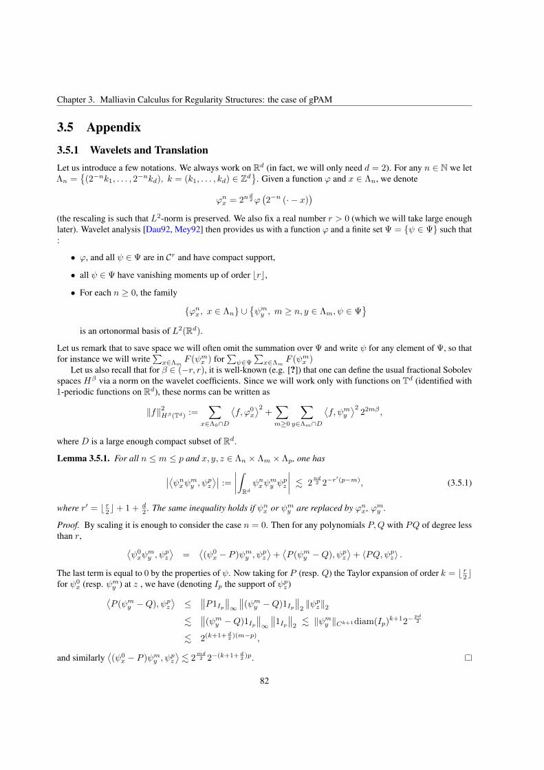
Chapter 3. Malliavin Calculus for Regularity Structures: the case of gPAM
3.5 Appendix
3.5.1 Wavelets and TranslationLet us introduce a few notations. We always work on Rd (in fact, we will only need d = 2). For any n ∈ N we letΛn =
(2−nk1, . . . , 2
−nkd), k = (k1, . . . , kd) ∈ Zd
. Given a function ϕ and x ∈ Λn, we denote
ϕnx = 2nd2ϕ2−n (· − x)
(the rescaling is such that L2-norm is preserved. We also fix a real number r > 0 (which we will take large enoughlater). Wavelet analysis [Dau92, Mey92] then provides us with a function ϕ and a finite set Ψ = ψ ∈ Ψ such that:
• ϕ, and all ψ ∈ Ψ are in Cr and have compact support,
• all ψ ∈ Ψ have vanishing moments up of order ⌊r⌋,
• For each n ≥ 0, the family
ϕnx , x ∈ Λn ∪ψmy , m ≥ n, y ∈ Λm, ψ ∈ Ψ
is an ortonormal basis of L2(Rd).
Let us remark that to save space we will often omit the summation over Ψ and write ψ for any element of Ψ, so thatfor instance we will write
x∈Λm
F (ψmx ) forψ∈Ψ
x∈Λm
F (ψmx )Let us also recall that for β ∈ (−r, r), it is well-known (e.g. [?]) that one can define the usual fractional Sobolev
spaces Hβ via a norm on the wavelet coefficients. Since we will work only with functions on Td (identified with1-periodic functions on Rd), these norms can be written as
∥f∥2Hβ(Td) :=
x∈Λ0∩D
f, ϕ0
x
2+m≥0
y∈Λm∩D
f, ψmy
222mβ ,
where D is a large enough compact subset of Rd.
Lemma 3.5.1. For all n ≤ m ≤ p and x, y, z ∈ Λn × Λm × Λp, one hasψnxψmy , ψpz := Rd
ψnxψmy ψ
pz
. 2nd2 2−r
′(p−m), (3.5.1)
where r′ = ⌊ r2⌋+ 1 + d2 . The same inequality holds if ψnx or ψmy are replaced by ϕnx , ϕmy .
Proof. By scaling it is enough to consider the case n = 0. Then for any polynomials P,Q with PQ of degree lessthan r,
ψ0xψ
my , ψ
pz
=
(ψ0x − P )ψmy , ψ
pz
+P (ψmy −Q), ψpz
+ ⟨PQ,ψpz⟩ .
The last term is equal to 0 by the properties of ψ. Now taking for P (resp. Q) the Taylor expansion of order k = ⌊ r2⌋for ψ0
x (resp. ψmy ) at z , we have (denoting Ip the support of ψpz )P (ψmy −Q), ψpz
≤
P1Ip∞ (ψmy −Q)1Ip2∥ψpz∥2
.(ψmy −Q)1Ip
∞
1Ip2 . ∥ψmy ∥Ck+1diam(Ip)k+12−
pd2
. 2(k+1+ d2 )(m−p),
and similarly(ψ0x − P )ψmy , ψ
pz
. 2
md2 2−(k+1+ d
2 )p.
82
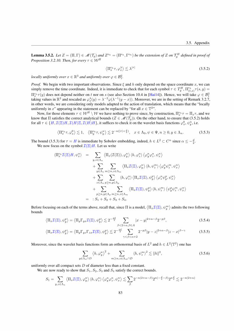
3.5. Appendix
Lemma 3.5.2. Let Z = (Π,Γ) ∈ M (Tg) and Zeh = (Πeh ,Γeh) be the extension of Z on T Hg defined in proof of
Proposition 3.2.10. Then, for every τ ∈ WH Πehx τ, ϕ
λx
. λ|τ | (3.5.2)
locally uniformly over x ∈ R3 and uniformly over ϕ ∈ B21 .
Proof. We begin with two important observations. Since ξ and h only depend on the space coordinate x, we cansimply remove the time coordinate. Indeed, it is immediate to check that for each symbol τ ∈ THg , Πeh(t,x)τ(s, y) =Πehx τ(y) does not depend neither on t nor on s (see also Section 10.4 in [Hai14]). Hence, we will take ϕ ∈ B2
1
taking values in R2 and rescaled as ϕλx(y) = λ−2ϕ(λ−1(y − x)). Moreover, we are in the setting of Remark 3.2.7,in other words, we are considering only models adapted to the action of translation, which means that the “locallyuniformly in x” appearing in the statement can be replaced by “for all x ∈ T2”.
Now, for those elements τ ∈ WH \W we have nothing to prove since, by construction, Πehx τ = Πxτ , and weknow that Π satisfies the correct analytical bounds (Z ∈ M (Tg)). On the other hand, to ensure that (3.5.2) holdsfor all τ ∈ H, I(Ξ)H, I(H)Ξ, I(H)H, it suffices to check it on the wavelet basis functions ϕ0
x, ψny , i.e.Πehx τ, ϕ
0x
. 1,
Πehy τ, ψ
ny
. 2−n(|τ |+
d2 ), x ∈ Λ0, ψ ∈ Ψ, n ≥ 0, y ∈ Λn. (3.5.3)
The bound (3.5.3) for τ = H is immediate by Sobolev embedding, indeed, h ∈ L2 ⊂ Cα since α ≤ −d2 .
We now focus on the symbol I(Ξ)H . Let us write
⟨Πehx I(Ξ)H,ψnx ⟩ =
y,z∈Λn
Πx(I(Ξ)), ϕny
⟨h, ϕnz ⟩
ϕnyϕ
nz , ψ
nx
+y∈Λn
m≥n,z∈Λm
ΠxI(Ξ), ϕny
⟨h, ψmz ⟩
ϕnyψ
mz , ψ
nx
+z∈Λn
p≥n,y∈Λp
⟨h, ϕnz ⟩ΠxI(Ξ), ψpy
ϕnzψ
py , ψ
nx
+
p≥n,y∈Λp
m≥n,z∈Λm
ΠxI(Ξ), ψpy
⟨h, ψmz ⟩
ψpyψ
mz , ψ
nx
= : S1 + S2 + S3 + S4.
Before focusing on each of the terms above, recall that, since Π is a model,ΠxI(Ξ), ψmy
admits the two following
bounds ΠxI(Ξ), ψpy
=ΠyΓyxI(Ξ), ψpy
. 2−
pd2
β<2+α,β∈A
|x− y|2+α−β2−pβ , (3.5.4)
ΠxI(Ξ), ψpy
=ΠyΓyzΓzxI(Ξ), ψpy
. 2−
pd2
γ<β<α+2
2−pβ |y − z|2+α−β |z − x|β−γ (3.5.5)
Moreover, since the wavelet basis functions form an orthonormal basis of L2 and h ∈ L2(T2) one hasy∈Λn∩D
h, ϕny
2+
m≥n,z∈Λm∩D
⟨h, ψmz ⟩2 . ∥h∥2, (3.5.6)
uniformly over all compact sets D of diameter less than a fixed constant.We are now ready to show that S1, S2, S3 and S4 satisfy the correct bounds.
S1 =
y,z∈Λn
ΠxI(Ξ), ϕny
⟨h, ϕnz ⟩
ϕnyϕ
nz , ψ
nx
.β
2−n(2+α−β)2n(−d2−β)2n
d2 . 2−n(2+α)
83
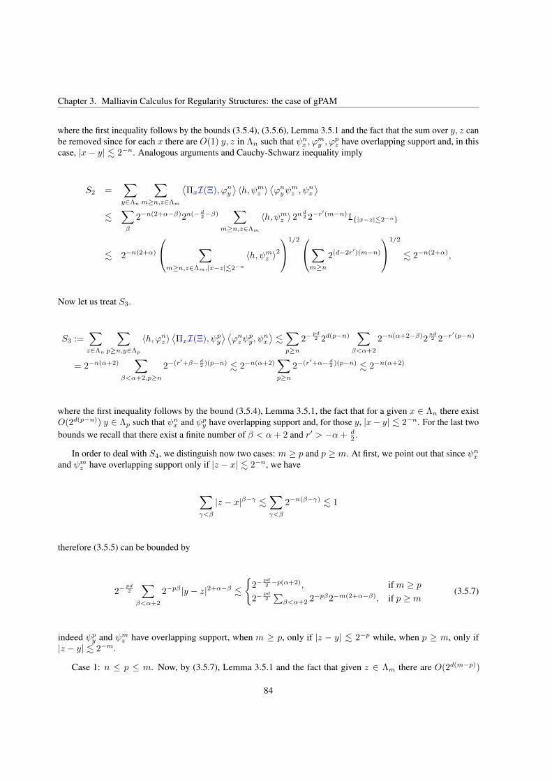
Chapter 3. Malliavin Calculus for Regularity Structures: the case of gPAM
where the first inequality follows by the bounds (3.5.4), (3.5.6), Lemma 3.5.1 and the fact that the sum over y, z canbe removed since for each x there are O(1) y, z in Λn such that ψnx , ϕ
my , ϕ
pz have overlapping support and, in this
case, |x− y| . 2−n. Analogous arguments and Cauchy-Schwarz inequality imply
S2 =y∈Λn
m≥n,z∈Λm
ΠxI(Ξ), ϕny
⟨h, ψmz ⟩
ϕnyψ
mz , ψ
nx
.
β
2−n(2+α−β)2n(−d2−β)
m≥n,z∈Λm
⟨h, ψmz ⟩ 2n d2 2−r
′(m−n)1|x−z|.2−n
. 2−n(2+α)
m≥n,z∈Λm,|x−z|.2−n
⟨h, ψmz ⟩21/2
m≥n
2(d−2r′)(m−n)
1/2
. 2−n(2+α),
Now let us treat S3.
S3 :=z∈Λn
p≥n,y∈Λp
⟨h, ϕnz ⟩ΠxI(Ξ), ψpy
ϕnzψ
py , ψ
nx
.p≥n
2−pd2 2d(p−n)
β<α+2
2−n(α+2−β)2nd2 2−r
′(p−n)
= 2−n(α+2)
β<α+2,p≥n
2−(r′+β− d2 )(p−n) . 2−n(α+2)
p≥n
2−(r′+α− d2 )(p−n) . 2−n(α+2)
where the first inequality follows by the bound (3.5.4), Lemma 3.5.1, the fact that for a given x ∈ Λn there existO(2d(p−n)) y ∈ Λp such that ψnx and ψpy have overlapping support and, for those y, |x− y| . 2−n. For the last twobounds we recall that there exist a finite number of β < α+ 2 and r′ > −α+ d
2 .
In order to deal with S4, we distinguish now two cases: m ≥ p and p ≥ m. At first, we point out that since ψnxand ψmz have overlapping support only if |z − x| . 2−n, we have
γ<β
|z − x|β−γ .γ<β
2−n(β−γ) . 1
therefore (3.5.5) can be bounded by
2−pd2
β<α+2
2−pβ |y − z|2+α−β .
2−
pd2 −p(α+2), if m ≥ p
2−pd2
β<α+2 2
−pβ2−m(2+α−β), if p ≥ m(3.5.7)
indeed ψpy and ψmz have overlapping support, when m ≥ p, only if |z − y| . 2−p while, when p ≥ m, only if|z − y| . 2−m.
Case 1: n ≤ p ≤ m. Now, by (3.5.7), Lemma 3.5.1 and the fact that given z ∈ Λm there are O(2d(m−p))
84
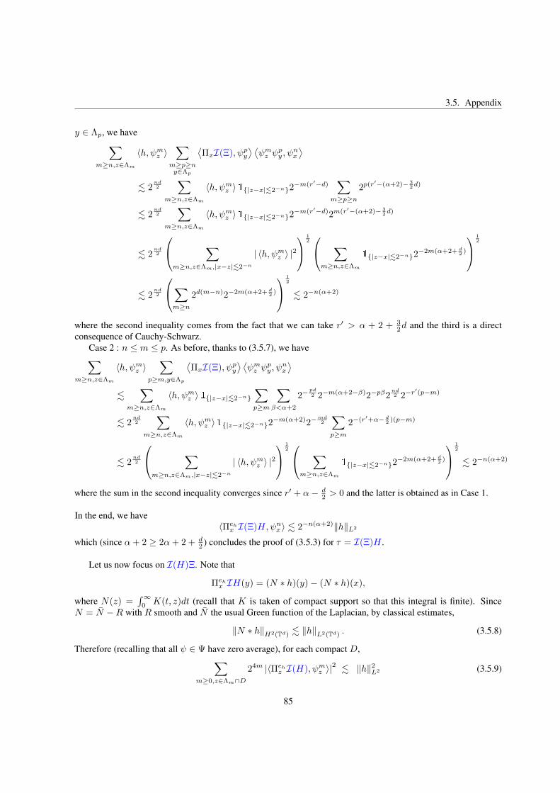
3.5. Appendix
y ∈ Λp, we havem≥n,z∈Λm
⟨h, ψmz ⟩
m≥p≥ny∈Λp
ΠxI(Ξ), ψpy
ψmz ψ
py , ψ
nx
. 2
nd2
m≥n,z∈Λm
⟨h, ψmz ⟩1|z−x|.2−n2−m(r′−d)
m≥p≥n
2p(r′−(α+2)− 3
2d)
. 2nd2
m≥n,z∈Λm
⟨h, ψmz ⟩1|z−x|.2−n2−m(r′−d)2m(r′−(α+2)− 3
2d)
. 2nd2
m≥n,z∈Λm,|x−z|.2−n
| ⟨h, ψmz ⟩ |2 1
2 m≥n,z∈Λm
1|z−x|.2−n2−2m(α+2+ d
2 )
12
. 2nd2
m≥n
2d(m−n)2−2m(α+2+ d2 )
12
. 2−n(α+2)
where the second inequality comes from the fact that we can take r′ > α + 2 + 32d and the third is a direct
consequence of Cauchy-Schwarz.Case 2 : n ≤ m ≤ p. As before, thanks to (3.5.7), we have
m≥n,z∈Λm
⟨h, ψmz ⟩
p≥m,y∈Λp
ΠxI(Ξ), ψpy
ψmz ψ
py , ψ
nx
.
m≥n,z∈Λm
⟨h, ψmz ⟩1|z−x|.2−np≥m
β<α+2
2−pd2 2−m(α+2−β)2−pβ2
nd2 2−r
′(p−m)
. 2nd2
m≥n,z∈Λm
⟨h, ψmz ⟩1|z−x|.2−n2−m(α+2)2−
md2
p≥m
2−(r′+α− d2 )(p−m)
. 2nd2
m≥n,z∈Λm,|x−z|.2−n
| ⟨h, ψmz ⟩ |2 1
2 m≥n,z∈Λm
1|z−x|.2−n2−2m(α+2+ d
2 )
12
. 2−n(α+2)
where the sum in the second inequality converges since r′ + α− d2 > 0 and the latter is obtained as in Case 1.
In the end, we have⟨Πehx I(Ξ)H,ψnx ⟩ . 2−n(α+2)∥h∥L2
which (since α+ 2 ≥ 2α+ 2 + d2 ) concludes the proof of (3.5.3) for τ = I(Ξ)H .
Let us now focus on I(H)Ξ. Note that
Πehx IH(y) = (N ∗ h)(y)− (N ∗ h)(x),
where N(z) =∞0K(t, z)dt (recall that K is taken of compact support so that this integral is finite). Since
N = N −R with R smooth and N the usual Green function of the Laplacian, by classical estimates,
∥N ∗ h∥H2(Td) . ∥h∥L2(Td) . (3.5.8)
Therefore (recalling that all ψ ∈ Ψ have zero average), for each compact D,m≥0,z∈Λm∩D
24m |⟨Πehz I(H), ψmz ⟩|2 . ∥h∥2L2 (3.5.9)
85
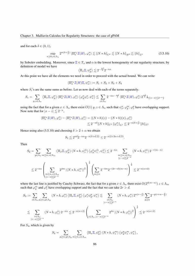
Chapter 3. Malliavin Calculus for Regularity Structures: the case of gPAM
and for each δ ∈ (0, 1),
supn≥0,x∈Λn
2n(δ+d2 ) ⟨Πehx I(H), ϕnx⟩ . ∥N ∗ h∥Cδ . ∥N ∗ h∥H2 . ∥h∥L2 (3.5.10)
by Sobolev embedding. Moreover, since Ξ ∈ Tα and α is the lowest homogeneity of our regularity structure, bydefinition of model we have
ΠxΞ, ψpy
. 2−
pd2 2−nα
At this point we have all the elements we need in order to proceed with the actual bound. We can write
⟨Πehx I(H)Ξ, ψnx ⟩ := S1 + S2 + S3 + S4
where Si’s are the same sums as before. Let us now deal with each of the terms separately.
S1 =
y,z∈Λn
ΠxΞ, ϕ
ny
⟨Πehx I(H), ϕnz ⟩
ϕnyϕ
nz , ψ
nx
.z∈Λn
2−nα−nd2 ⟨Πehx I(H), ϕnz ⟩ 2
nd2 1|z−x|.2−n
using the fact that for a given x ∈ Λn there exist O(1) y, z ∈ Λn such that ψnx , ϕmy , ϕ
pz have overlapping support.
Now note that for |x− z| . 2−n,
⟨Πehx I(H), ϕnz ⟩ − ⟨Πehz I(H), ϕnz ⟩ = ⟨(N ∗ h)(z)− (N ∗ h)(x), ϕnz ⟩
. 2−nδ∥N ∗ h∥Cδ ∥ϕnz ∥L1 . 2−n(δ+d2 )∥h∥L2
Hence using also (3.5.10) and choosing δ > 2 + α we obtain
S1 . 2nd2−nα2−n(δ+d/2) ≤ 2−n(2+2α+d/2).
Then
S2 =y∈Λn
m≥n,z∈Λm
ΠxΞ, ϕ
ny
⟨N ∗ h, ψmz ⟩
ϕnyψ
mz , ψ
nx
. 2−nα
m≥n,z∈Λm
|z−x|.2−n
⟨N ∗ h, ψmz ⟩ 2−r(m−n)
. 2−nα
m≥n,z∈Λm
|z−x|.2−n
24m |⟨N ∗ h, ψmz ⟩|2
12
m≥n
2−4m2−(2r−d)(m−n)
12
. 2−n(α+2)
where the last line is justified by Cauchy-Schwarz, the fact that for a given x ∈ Λn there exist O(2d(m−n)) z ∈ Λmsuch that ϕmy and ϕpz have overlapping support and the fact that we can take 2r > d.
S3 :=z∈Λn
p≥n,y∈Λp
⟨N ∗ h, ϕnz ⟩ΠxΞ, ψ
py
ϕnzψ
py , ψ
nx
.
z∈Λn
|z−x|.2−n
⟨N ∗ h, ϕnz ⟩ 2n(r−d2 )p≥n
2−p(r+α−d2 )
.z∈Λn
|z−x|.2−n
⟨N ∗ h, ϕnz ⟩ 2−nα . 2−n(α+2)
z∈Λn,|z−x|.2−n
24n |⟨N ∗ h, ϕnz ⟩|2
12
. 2−n(α+2)
For S4, which is given by
S4 =
p≥n,y∈Λp
m≥n,z∈Λm
ΠxΞ, ψ
py
⟨N ∗ h, ψmz ⟩
ψpyψ
mz , ψ
nx
,
86
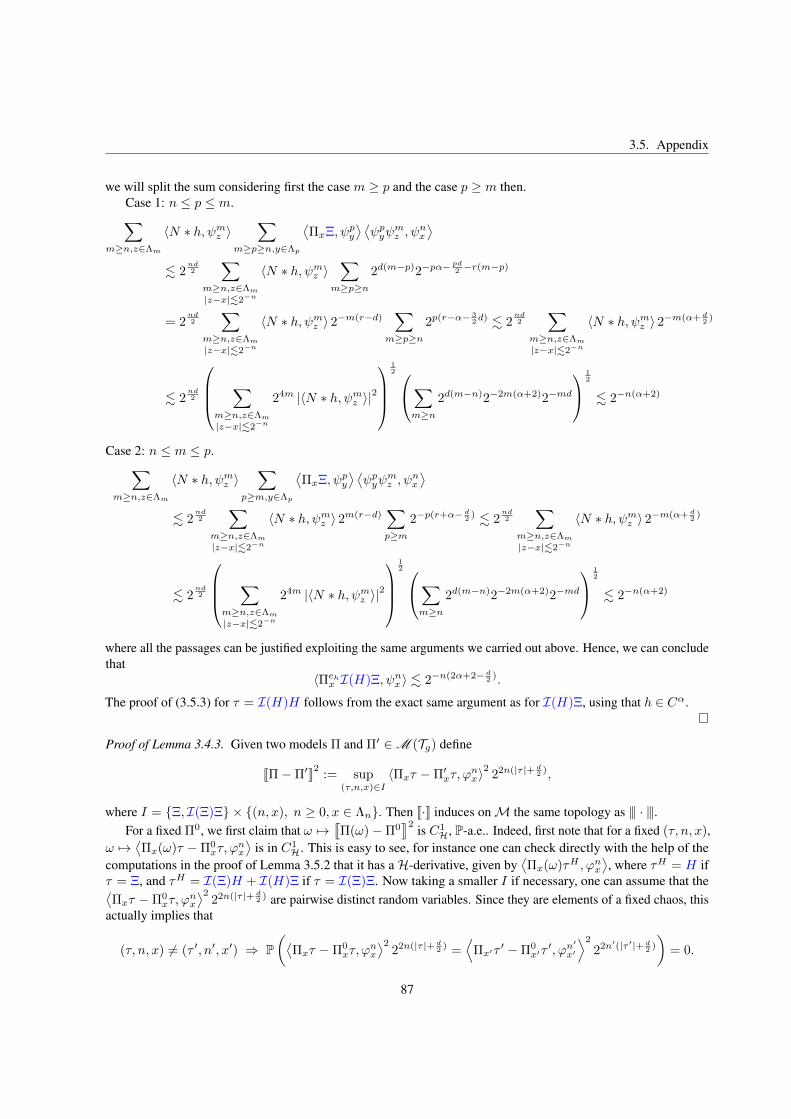
3.5. Appendix
we will split the sum considering first the case m ≥ p and the case p ≥ m then.Case 1: n ≤ p ≤ m.
m≥n,z∈Λm
⟨N ∗ h, ψmz ⟩
m≥p≥n,y∈Λp
ΠxΞ, ψ
py
ψpyψ
mz , ψ
nx
. 2
nd2
m≥n,z∈Λm
|z−x|.2−n
⟨N ∗ h, ψmz ⟩
m≥p≥n
2d(m−p)2−pα−pd2 −r(m−p)
= 2nd2
m≥n,z∈Λm
|z−x|.2−n
⟨N ∗ h, ψmz ⟩ 2−m(r−d)
m≥p≥n
2p(r−α−32d) . 2
nd2
m≥n,z∈Λm
|z−x|.2−n
⟨N ∗ h, ψmz ⟩ 2−m(α+ d2 )
. 2nd2
m≥n,z∈Λm
|z−x|.2−n
24m |⟨N ∗ h, ψmz ⟩|2
12
m≥n
2d(m−n)2−2m(α+2)2−md
12
. 2−n(α+2)
Case 2: n ≤ m ≤ p.m≥n,z∈Λm
⟨N ∗ h, ψmz ⟩
p≥m,y∈Λp
ΠxΞ, ψ
py
ψpyψ
mz , ψ
nx
. 2
nd2
m≥n,z∈Λm
|z−x|.2−n
⟨N ∗ h, ψmz ⟩ 2m(r−d)p≥m
2−p(r+α−d2 ) . 2
nd2
m≥n,z∈Λm
|z−x|.2−n
⟨N ∗ h, ψmz ⟩ 2−m(α+ d2 )
. 2nd2
m≥n,z∈Λm
|z−x|.2−n
24m |⟨N ∗ h, ψmz ⟩|2
12
m≥n
2d(m−n)2−2m(α+2)2−md
12
. 2−n(α+2)
where all the passages can be justified exploiting the same arguments we carried out above. Hence, we can concludethat
⟨Πehx I(H)Ξ, ψnx ⟩ . 2−n(2α+2− d2 ).
The proof of (3.5.3) for τ = I(H)H follows from the exact same argument as for I(H)Ξ, using that h ∈ Cα.
Proof of Lemma 3.4.3. Given two models Π and Π′ ∈ M (Tg) define
JΠ−Π′K2 := sup(τ,n,x)∈I
⟨Πxτ −Π′xτ, ϕ
nx⟩
222n(|τ |+
d2 ),
where I = Ξ, I(Ξ)Ξ × (n, x), n ≥ 0, x ∈ Λn. Then J·K induces on M the same topology as ||| · |||.For a fixed Π0, we first claim that ω →→
qΠ(ω)−Π0
y2is C1
H, P-a.e.. Indeed, first note that for a fixed (τ, n, x),ω →→
Πx(ω)τ −Π0
xτ, ϕnx
is in C1
H. This is easy to see, for instance one can check directly with the help of thecomputations in the proof of Lemma 3.5.2 that it has a H-derivative, given by
Πx(ω)τ
H , ϕnx, where τH = H if
τ = Ξ, and τH = I(Ξ)H + I(H)Ξ if τ = I(Ξ)Ξ. Now taking a smaller I if necessary, one can assume that theΠxτ −Π0
xτ, ϕnx
222n(|τ |+
d2 ) are pairwise distinct random variables. Since they are elements of a fixed chaos, this
actually implies that
(τ, n, x) = (τ ′, n′, x′) ⇒ P
Πxτ −Π0xτ, ϕ
nx
222n(|τ |+
d2 ) =
Πx′τ ′ −Π0
x′τ ′, ϕn′
x′
222n
′(|τ ′|+ d2 )
= 0.
87

Chapter 3. Malliavin Calculus for Regularity Structures: the case of gPAM
In additionΠxτ −Π0
xτ, ϕnx
2n(|τ |+
d2 ) goes to 0 as n→ ∞ for models in the closure of smooth functions, so that
the supremum in the definition ofqΠ(ω)−Π0
yis P-a.e. attained at a single (τ, x, n). Recalling that if ℓ∞0 is the
set of sequences going to 0 as n → ∞, the map (un)n≥0 ∈ ℓ∞0 →→ (supn≥0 un) is Frechet differentiable at eachsequence (un) attaining its supremum at a single point, this proves the claim.
Now fix a smooth function ψ on [0,+∞) such that ψ ≡ 1 on [0, 1] and ψ ≡ 0 on [2,+∞). Then, for fixedΠ0 ∈ M (Tg), δ0 > 0, define a function FΠ0,δ0 on M (Tg) by
FΠ0,δ0(Π) = ψ
1
δ0JΠ−Π0K
.
Then take a sequence (Πn) which is dense in t < T∞. Since t < T∞ is open, there exists δn > 0 such thatΠ ∈ M (Tg) : JΠ−ΠnK ≤ 3δn ⊂ t < T∞. Then Xn(ω) = FΠn,δn(Π(ω)) satisfies the required conditions.Indeed, it is clear by Theorem 3.3.11 that FXn ∈ C1
H−loc on t < T∞, with D(FXn) = FDXn +XnDF . Onthe other hand, from the properties of ψ it is clear that if ω /∈ t < T∞, then FΠn,δn(Π
′) = 0 for JΠ′ −ΠnK ≤ δn.In particular, for ∥h∥H small enough,Xn(ω+h) = 0, so that FXn is also H-differentiable at ω, withD(FXn) = 0.
3.5.2 Admissible Models and ConsistencyWe collect in this Appendix the proof of Remark 3.2.5 and Lemma 3.2.22.
Proof of Remark 3.2.5. We want to show that the second analytical bound in (3.2.5) automatically hold, given thatthe pair (Π,Γ) satisfies the first as well as the equalities (3.2.6) and (3.2.9). Notice that in the specific context of Tgwe have an explicit expression for Γxyτ for all τ ∈ Tg . While for τ = Ξ, 1, Xi it is oblvious, for the others we seethat
ΓxyI(Ξ)Ξ = I(Ξ)Ξ + (fy(J (Ξ))− fx(J (Ξ)))Ξ
ΓxyXiΞ = XΞ + (fy(Xi)− fx(Xi))Ξ
ΓxyI(Ξ) = I(Ξ) + (fy(J (Ξ))− fx(J (Ξ)))1
Now, ∥ΓxyXiΞ∥α . ∥x− y∥ is an obvious consequence of (3.2.6a), while, for the others, showing that ∥Γxyτ∥β .∥x− y∥|τ |−β , boils down to prove
|fy(J (Ξ))− fx(J (Ξ))| = |⟨ΠxΞ,K(x− ·)⟩ − ⟨ΠyΞ,K(y − ·)⟩| . ∥x− y∥α+2
But this bound is a bound on the map Π itself and can be easily obtained upon using the decomposition of thekernel, splitting the cases ∥x− y∥ . 2−1 and ∥x− y∥ > 2−1 and applying Proposition A.1 in [Hai14] and the firstanalytical bound in (3.2.5).
In the proof of lemma 3.2.22, we will make use of the actual definition of the reconstruction map (see Theorem3.10 in [Hai14] and, in particular, the bound (3.3)) and of the abstract heat kernel (see equations (5.11), (5.15),(5.16) and (7.7) in [Hai14]), but since this is the only point in which we will actually need them, we refrain in thiscontext from thoroughly explaining their structure and address the interested reader to the quoted reference.
Proof of Lemma 3.2.22. The first point in the previous is a direct consequence of the properties of τH . Moreprecisely, it is due to the fact that according to Remark 3.2.11, τH leaves the homogeneity invariant, and that, byconstruction, is linear and multiplicative.
For the second, the image of Tg through the canonical immersion map is a sector of T Hg . Since, the extended
model coincides with the original one on Tg , the bound (3.3) in the Reconstruction theorem in [Hai14] guaranteesthat also the two reconstruction maps coincide on the elements of Dγ for any γ > 0, and consequently, thanks toProposition 6.9 in [Hai14], on the ones of Dγ,η for η ∈ (−2, γ]. Analogously, one can prove that RehτH(Uh) =
88
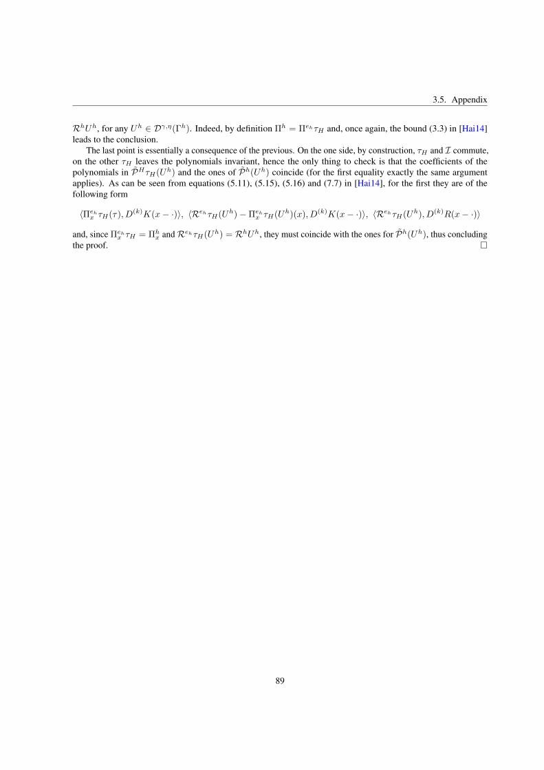
3.5. Appendix
RhUh, for any Uh ∈ Dγ,η(Γh). Indeed, by definition Πh = ΠehτH and, once again, the bound (3.3) in [Hai14]leads to the conclusion.
The last point is essentially a consequence of the previous. On the one side, by construction, τH and I commute,on the other τH leaves the polynomials invariant, hence the only thing to check is that the coefficients of thepolynomials in PHτH(Uh) and the ones of Ph(Uh) coincide (for the first equality exactly the same argumentapplies). As can be seen from equations (5.11), (5.15), (5.16) and (7.7) in [Hai14], for the first they are of thefollowing form
⟨Πehx τH(τ), D(k)K(x− ·)⟩, ⟨RehτH(Uh)−Πehx τH(Uh)(x), D(k)K(x− ·)⟩, ⟨RehτH(Uh), D(k)R(x− ·)⟩
and, since Πehx τH = Πhx and RehτH(Uh) = RhUh, they must coincide with the ones for Ph(Uh), thus concludingthe proof.
89

Chapter 3. Malliavin Calculus for Regularity Structures: the case of gPAM
90
Bibliography
[AKQ14] ALBERTS, T., KHANIN, K. and QUASTEL, J. The continuum directed random Polymer J. Stat. Phys.154,no. 1 (2014), 119–141.
[BCD11] H. BAHOURI, J.-Y. CHEMIN, and R. DANCHIN. Fourier analysis and nonlinear partial differentialequations, vol. 343 of Grundlehren der Mathematischen Wissenschaften [Fundamental Principles ofMathematical Sciences]. Springer, Heidelberg, 2011. doi:10.1007/978-3-642-16830-7.
[BC01] BASS, R., and CHEN, Z. Q. Stochastic differential equations for Dirichlet processes. Probab. Theory andRelated Fields 121, (2001), 422-446.
[Bony81] BONY, J.-M. Calcul symbolique et propagation des singularites pour les equations aux derivees partiellesnon lineaires Ann. Sci. Ecole Norm. Sup. no. 14 (1981), 209-246.
[BH86] BOULEAU, N., and HIRSCH, F. Proprietes dabsolue continuite dans les espaces de Dirichlet et applicationsaux equations differentielles stochastiques Lecture Notes in Math. 1204, (1986), 131-161.
[CC15] CANNIZZARO, G., and CHOUK, K., Multidimensional SDEs with singular drift and universal constructionof the polymer measure with white noise potential arXiv:1501.04751, (2015).
[CFG15] CANNIZZARO, G., FRIZ, P.K., and GASSIAT, P., Malliavin Calculus for regularity structures: the caseof gPAM arXiv:1511.08888, (2015).
[CF10] CASS, T., and FRIZ, P. Densities for rough differential equations under Hormander’s condition Annals ofMathematics 171,no. 3 (2010), 2115–2141.
[CF11] CASS, T., and FRIZ, P. Malliavin Calculus and Rough Paths Bull. Sci. Math. 135,no. 6-7 (2011), 542–556.
[CFV09] CASS, T., FRIZ, P., and VICTOIR, N. Non-degeneracy of Wiener functionals arising from roughdifferential equations Trans. Amer. Math. Soc. 361,no. 6 (2009), 3359–3371.
[CHLT15] CASS, T., HAIRER, M., LITTERER, C. and TINDEL, S. Smoothness of the density for solutions toGaussian rough differential equations Ann. Probab. 43,no. 1 (2015), 188–239.
[CC13] CATELLIER, R., and CHOUK, K., Paracontrolled Distributions and the 3-dimensional Stochastic Quanti-zation Equation arXiv:1310.6869, (2013).
[CW15] A. CHANDRA, and H. WEBER. Stochastic PDES, Regularity Structures, and interacting particle systemsarXiv:1508.03616.
[Dau92] DAUBECHIES, I. Ten lectures on wavelets. CBMS-NSF Regional Conference Series in Applied Mathe-matics, Society for Industrial and Applied Mathematics (SIAM), Philadelphia, (PA) (1992)
91
Bibliography
[DD14] DELARUE, F., and DIEL, R., Rough paths and 1d sde with a time dependent distributional drift. Applicationto polymers arXiv:1402.3662v2, (2014).
[DT13] DEYA, A., and TINDEL, S. Malliavin Calculus for Fractional Heat Equation Malliavin calculus andstochastic analysis 34 (2013), 361-384.
[BD03] DRIVER, B.K. Analysis Tools with Applications. Springer, 2003
[EK86] ETHIER, S. N., and KURTZ, T.G., Markov Processes, Characterization and Convergence. Wiley Seriesin Probability and Mathematical Statistics, 120, John Wiley & Sons, Inc., New York, (1986).
[FIR14] FLANDOLI, F., ISSOGLIO, E. and RUSSO, F. Multidimensional stochastic differential equations withdistributional drift arXiv:1401.6010, (2014).
[FRW03] FLANDOLI, F., RUSSO, F. and WOLF, J. Some SDEs with distributional drift. I. General calculus. OsakaJ. of Math., 40, (2003), 493542.
[FRW04] FLANDOLI, F., RUSSO, F. and WOLF, J. Some SDEs with distributional drift. II. Lyons-Zheng structure,Itos formula and semimartingale characterization Random Oper. Stochastic Equations, 2, (2004), 145-184.
[FGGR] FRIZ, P. K., GESS, B., GULISASHVILI, A. and RIEDEL, S. The Jain-Monrad criterion for rough pathsand applications to random Fourier series and non-Markovian Hormander theory Ann. Probab. (accepted)(2014).
[FH14] FRIZ, P.K., and HAIRER, M., A Course on Rough Paths: With an Introduction to Regularity Structures.Springer Universitext. Springer, 2014
[FV06] FRIZ, P., and VICTOIR, N.B. A variation embedding theorem and applications J. Funct. Anal. 239, no. 2(2006), 631–637.
[FV10] P.K. FRIZ, and VICTOIR, N.B., Multidimensional stochastic processes as rough paths. Cambridge Studiesin Advanced Mathematics 120, Theory and applications, Cambridge University Press, Cambridge (2010)
[GRR70] GARSIA, A.M., RODEMICH, E., and RUMSEY, H.. A real variable lemma and the continuity of paths ofsome Gaussian processes. Indiana Univ. Math. J. 20, no. 6, (1970), 565–578.
[Gub04] M. GUBINELLI, Controlling rough paths Journal of Functional Analysis 216, no. 1, (2004), 86–140.
[GP15] M. GUBINELLI, and N. PERKOWSKI. KPZ Reloaded. arXiv:1508.03877.
[GIP15a] M. GUBINELLI, P. IMKELLER, and N. PERKOWSKI. Paracontrolled distributions and singular PDEs.Forum of Mathematics, Pi 3, no. 6, (2015), 1–75. arXiv:1210.2684.
[GIP15b] M. GUBINELLI, P. IMKELLER, and N. PERKOWSKI. A Fourier approach to pathwise stochasticintegration. arXiv:1410.4006.
[Hai13] M. HAIRER. Solving the KPZ equation, Annals of Mathematics 178, no. 2, (2013), 559-664. arXiv:1109.6811.
[Hai14] M. HAIRER. A theory of Regularity Structures. Inventiones mathematicae 198, no. 2, (2015), 1-236.arXiv:1303.5113.
[Hai15] M. HAIRER. Introduction to Regularity Structures. arXiv:1401.3014.
[HL15a] M. HAIRER and LABBE, C., A simple construction of the continuum parabolic Anderson model on R2.arXiv:1501.00692, (2015).
92
Bibliography
[HL15b] M. HAIRER and LABBE, C. Multiplicative stochastic heat equations on the whole space. arXiv:1504.07162, (2015).
[HM15] M. HAIRER and K. MATETSKI. Discretisations of rough stochastic pdes, arXiv:1511.06937, (2015).
[HP14] M. HAIRER and PARDOUX, E. A Wong-Zakai theorem for stochastic PDEs. J. Math. Soc. Japan 67, no. 4,(2015), 1151–1604. arXiv:1409.3138, (2014).
[HW15] M. HAIRER and WEBER, H. Large deviations for white-noise driven, nonlinear stochastic PDEs intwo and three dimensions. Annales de la Facult des Sciences de Toulouse 24(6), no. 1, (2015), 55–92.arXiv:1409.3138, (2014).
[Jan97] JANSON, S.. Foundations of modern probability. Probability and its Applications (New York). Springer-Verlag, New York, second ed., 2002.
[Kal02] O. KALLENBERG. Gaussian Hilbert Spaces. Cambridge University Press, (1997).
[KPZ86] KARDAR, M., PARISI, G. and ZHANG, Y.-C.. Dynamic scaling of growing interfaces. Phys. Rev. Lett.56, no. 9 (1986), 889-892.
[KZ65] M.D. KRUSKAL, and N.J.ZABUSKY. Exact statistical properties of the Burgers equation. Phys. Rev. Lett.15, (1965), 240-243.
[KR05] KRYLOV, N. V. and ROCKNER, M.. Strong solutions of stochastic equations with singular time dependentdrift. Probab. Theory and Related Fields 131, 154-196.
[Kus93] KUSUOKA, K.. On the regularity of solutions to SDE. Asymptotic problems in probability theory: Wienerfunctionals and asymptotics (Sanda/Kyoto, 1990), Pitman Res. Notes Math. Ser.284, Longman Sci. Tech.,Harlow (1993), 90–103.
[Lyo98] LYONS, TERRY J., Differential equations driven by rough signals. Rev. Mat. Iberoamericana 14, no. 2,(1998), 215–310.
[Mal97] MALLIAVIN, P.. Stochastic analysis, vol. 313 of Grundlehren der Mathematischen Wissenschaften[Fundamental Principles of Mathematical Sciences]. Springer-Verlag, Berlin, (1997).
[Mey92] Y. MEYER. Wavelets and operators, vol. 37 of Cambridge Studies in Advanced Mathematics. CambridgeUniversity Press, Cambridge, (1992).
[MW15] MOURRAT J.-C. and WEBER H.. Global well-posedness of the dynamic Φ4 model in the plane,arXiv:1501.06191v1, (2015).
[MW16] MOURRAT J.-C. and WEBER H.. Global well-posedness of the dynamic Φ43 model on the torus,
arXiv:1601.01234, (2016).
[Mue91] MUELLER, C., On the support of solutions to the heat equation with noise. Stochastics and StochasticReports 37, no. 4, (1991), 225–245.
[Nua06] D. NUALART. The Malliavin calculus and related topics. Probability and its Applications (New York).Springer-Verlag, Berlin, second ed., 2006.
[NS09] NUALART, D., and SAUSSEREAU, B.. Malliavin Calculus for stochastic differential equations driven byfractional Brownian motion. Stochastic Process. Appl. 119 (2), (2009), 391-409.
[San05] SANZ-SOLE, M., Malliavin Calculus. Fundamental Sciences, With applications to stochastic partialdifferential equations, EPFL Press, Lausanne; distributed by CRC Press, Boca Raton, FL, (2005).
93

Bibliography
[Str10] STROOCK, D.W.. Probability Theory, An Analytic View (2nd Edition) Cambridge University Press,Cambridge, (1992).
[UZ00] UESTUENEL, A. S., and ZAKAI, M.. Transformation of measure on Wiener space Springer-Verlag, Berlin(2000).
[ZZ15] ZHU, R. , and ZHU, X. . Three-dimensional Navier-Stokes equations driven by space-time white noise.arXiv:1406.0047, (2015).
94