site selection by migratory shorebirds in oregon estuaries
TRANSCRIPT

Portland State University Portland State University
PDXScholar PDXScholar
Dissertations and Theses Dissertations and Theses
Fall 11-29-2012
Site Selection by Migratory Shorebirds in Oregon Site Selection by Migratory Shorebirds in Oregon
Estuaries Over Broad and Fine Spatial Scales Estuaries Over Broad and Fine Spatial Scales
Aileen Kilpatrick Miller Portland State University
Follow this and additional works at: https://pdxscholar.library.pdx.edu/open_access_etds
Part of the Ornithology Commons, and the Other Environmental Sciences Commons
Let us know how access to this document benefits you.
Recommended Citation Recommended Citation Miller, Aileen Kilpatrick, "Site Selection by Migratory Shorebirds in Oregon Estuaries Over Broad and Fine Spatial Scales" (2012). Dissertations and Theses. Paper 443. https://doi.org/10.15760/etd.443
This Thesis is brought to you for free and open access. It has been accepted for inclusion in Dissertations and Theses by an authorized administrator of PDXScholar. Please contact us if we can make this document more accessible: [email protected].

Site Selection by Migratory Shorebirds in Oregon Estuaries
Over Broad and Fine Spatial Scales
by
Aileen Kilpatrick Miller
A thesis submitted in partial fulfillment of the
requirements for the degree of
Master of Science
in
Environmental Science and Management
Thesis Committee:
Catherine de Rivera, Chair
Michael Murphy
Greg Ruiz
Portland State University
2012

i
Abstract
Many migratory shorebirds rely on estuaries as stop-over sites to refuel during
migration, and the loss of stop-over sites is a primary threat to shorebird populations on
the West Coast of the United States (e.g. Calidris alpina pacifica, C. mauri).
Conservation and research has focused on the largest of these sites; however, smaller
estuaries also host thousands of migratory shorebirds. Furthermore, the reasons for
site selection are largely unknown. Estuarine inter-tidal microhabitats are non-uniform
and both abiotic and biotic factors may serve as predictors of whether an abundance of
shorebirds will use a site. I investigated shorebird site selection on broad and fine scales
within Oregon estuaries.
To identify factors that relate to shorebird abundance on large spatial scales, I
compiled shorebird abundance data from estuaries throughout the Pacific Northwest as
well as data on site quality factors. To investigate site selection on a finer scale I
measured shorebird abundance, habitat characteristics, and food
resources―invertebrates and a newly considered source, biofilm―within two Oregon
estuaries during the fall migration period. Finally, I examined whether channels are
preferentially used by foraging Calidrid shorebirds by conducting observations during
the spring migration. I investigated whether channels may be superior foraging habitat
possibly because prey are more abundant, are found at shallower depths, or because
sediments are more penetrable (increasing the opportunity for shorebird probing) by

ii
taking infauna cores and measuring force required to probe in the sediment at channel
and open mudflat sites.
Among estuaries, shorebird densities in spring were best predicted by estuary
size, as opposed to the amount of any one habitat. During fall migration, the amount of
grassland in the surrounding watershed was also a good predictor, pointing to the
probable importance of roost sites as well as feeding grounds. The amount of infauna
also related to the density of shorebirds using a site. Within estuaries, shorebird
distribution in the inter-tidal region was not generally predicted by prey abundance.
Channels were used preferentially by shorebirds, and infauna abundance along channels
was greater than in the surrounding mudflats. The more penetrable sediments of the
channel also made it easier for shorebirds to probe and capture prey. Identification of
these large-scale and fine-scale factors that influence site quality for migratory
shorebirds will assist land and wildlife managers’ efforts to protect these species.
iii
Acknowledgements
I am extremely grateful to the individuals and organizations who have supported my
thesis research with intellectual, practical, and financial support. My initial interest in
this project developed from work with The Wetlands Conservancy including Esther Lev,
John Bauer and John Christie.
Shorebird abundance and distribution data that were the foundation of my
analysis in Chapter 1 were provided by Lynne Stenzel and PRBO Conservation Science. I
thank the staff at PRBO and the many volunteers who conducted these extensive
shorebird surveys. I also appreciate access to environmental data collected by the US
EPA Western Ecology Division including both previously published data and data
supplied by Melanie Frazier and Walt Nelson. Early development of the project also
benefitted from discussions with Janet Lamberson of the US EPA.
My research in Bandon Marsh was possible because of logistical support and
permits from USFWS. Bill Bridgeland, Dave Ledig and Ben Wishnek at Bandon Marsh
National Wildlife Refuge offered excellent advice and support for my research. Ben
Wishnek conducted the avian transect surveys I report on in Chapter 2.
I could not have completed this project without the excellent help I had in the
lab and in the field. Nicole Veenker sorted infauna samples along with help from
Daphne Cissell. Basma Mohammad, Sara Henderson, Michael Smith, Shelly Hsu, Mariah
Muller and Nicole Veenker all spent time slogging through the mud with me collecting
samples. Joan Miller helped with technical editing of data and of this thesis.

iv
I was able to analyze chlorophyll a and ash-free dry mass measurements using
the labs of Dr. Mark Sytsma, Dr. Alan Yeakley, and Dr. Yangdong Pan. Steve Wells, Rich
Miller, and Chris Parker taught me these techniques and generously loaned equipment.
My committee members, Dr. Michael Murphy and Dr. Greg Ruiz, provided
insightful feedback on earlier drafts of my thesis. Finally, I want to thank my advisor
Catherine de Rivera for extensive help throughout this project. She contributed
substantially to the study design, set-up, analysis and interpretation.

v
Table of Contents
Abstract ........................................................................................................................ i
Acknowledgements .................................................................................................... iii
List of Tables ............................................................................................................... vi
List of Figures ............................................................................................................ viii
Background and Objectives ....................................................................................... 1
Chapter 1. Shorebird site quality and selection among Pacific Northwest
Estuaries...................................................................................................................... 4
Chapter 2. Shorebird numerical responses to prey distribution within Oregon
estuaries ................................................................................................................... 24
Chapter 3. Small tidal channels improve foraging opportunities for Calidris
shorebirds ................................................................................................................. 51
Conclusions ............................................................................................................... 72
References ................................................................................................................ 74

vi
List of Tables
Table 1.1. Data used in analysis and sources. X indicates that the particular data type
was available for that estuary. San Francisco Bay was not included in analysis, but
shorebird and infauna density were included as a comparison point. RE=river estuary.
Table 1.2. Density of shorebirds (±SD) in each PNW estuary for spring and fall 1990-
1995. Estuaries are listed from north to south. Sample size indicates the number of
years counts were conducted for that season and estuary. RE=river estuary.
Table 1.3. Shorebird abundance in relation to total estuary area, estuary habitat
composition (%Flats, %Marsh, or %Flats+%Marsh), or watershed land use
(%Development, %Grassland & Agriculture, or %Development + %Grassland &
Agriculture). Linear regression model results. Comparisons were made for all PNW
estuaries and for only Oregon estuaries since habitat data was not available for either
Willapa Bay or Humboldt Bay. Model in bold has the lowest AIC value.
Table 1.4. Infauna and shorebird density for PNW Estuaries. Infauna is calculated as
density per 0.01m2. Cores were of differing depths, but ~90% of infauna live in the top
3 cm so this difference should introduce only a small bias. Actual core depth given with
source.
Table 2.1. Infauna abundance (mean ± SD) in the four regions of Tillamook Bay, OR,
from three 4cm diameter x 3 cm deep cores. "Unknown" includes species that could not
be identified either because they were rare or because they had been damaged.
Table 2.2. Models of shorebird abundance in relation to infauna abundance and biofilm
indicators, ash-free dry mass (AFDM) and chlorophyll a (CHLA) from surface sediment.
Table 2.3. Infauna abundance (mean number of individuals ± SD) in Bandon Marsh, OR,
from three 4cm diameter x 3 cm deep cores. "Unknown" includes species that could not
be identified either because they were rare or because they had been damaged.
Table 2.4. Models of shorebird abundance in relation to infauna abundance and biofilm
indicators, ash-free dry mass (AFDM) and chlorophyll a (CHLA) from surface sediment.
Table 3.1. Multi-factor ANOVA results of infauna abundance in relation to depth in the
sediment (0-0.5cm,0.5-1.5cm,1-5-3cm), distance from channel (0m, 5m), and tide (ebb,
low). Non-significant interaction terms were removed. N=9 sites with samples of each
combination of the above treatments.

vii
Table 3.2. Total abundance of infauna (mean ± SD) in paired Channel and Non-channel
sites, and in Gracilaria habitat. Large infauna includes amphipods >2mm and
polychaetes >5mm.
viii
List of Figures
Figure 1.1. Composition of shorebird communities in PNW estuaries, 1990-1995 (PRBO
Conservation Science unpublished data; Page et al. 1999). Mean percent abundance of
each species (±SD).
Figure 2.1. Maps of Tillamook Bay, OR and Bandon Marsh, OR. Lines in red represent
survey transects.
Figure 2.2. Number of shorebirds and number of flocks by species seen per survey in
Tillamook Bay and Bandon Marsh, OR.
Figure 2.3. Density of shorebird groups and individuals by region in Tillamook Bay, OR.
Boxplot illustrates the median line, first and third quartile boxes and min and max value
hinges.
Figure 2.4. Infauna abundance and biofilm indicators, ash-free dry mass (AFDM) and
chlorophyll a (CHLA), by region in Tillamook Bay, OR. Boxplot illustrates the median line,
first and third quartile boxes and min and max value hinges with outliers excluded and
shown as circles.
Figure 2.5. Ordination of infauna samples based on community composition, labeled by
region, for Tillamook Bay, OR.
Figure 2.6. Infauna abundance and biofilm indicators, ash-free dry mass (AFDM) and
chlorophyll a (CHLA), in relationship to shorebird abundance per hectare plot in Bandon
Marsh, OR.
Figure 3.1. Relative density (percent per m2) of (a) Western Sandpiper flocks, (b)
Western Sandpiper individuals, (c) Dunlin flocks, and (d) Dunlin individuals by habitat
type. and log transformed. Letters indicate habitat types that differed significantly
based on post-hoc tests. N=7 observation dates. Boxplot illustrates the median line,
first and third quartile boxes and min and max value hinges with outliers excluded and
shown as circles.
Figure 3.2. Proportion of (a) Western Sandpipers and (b) Dunlin foraging along channels
in relation to tide height. Negative tide heights refer to ebb tides and positive height
refer to flow tides. Lines show fitted logistic regression models.
Figure 3.3. Proportion of Western Sandpiper foraging actions that were probes (as
opposed to pecks at the surface) along channels or in other habitats (red algae habitat
ix
excluded). Boxplot illustrates the median line, first and third quartile boxes and min and
max value hinges with outliers excluded and shown as circles.
Figure 3.4. Average abundance of (a) all infauna and (b) Corophiid amphipods in
relation to depth in the sediment, distance from channel and tide. Error bars represent
1 SE.
Figure 3.5. Average (a) abundance of infauna for all depths combined and (b) force
required to probe in the sediment. Channel and other habitats were from paired
samples taken 5m apart; random samples were collected separately for the red algae
microhabitat. Error bars show 1 SD.
1
Background and Objectives
Migration is a critical period for nearctic breeding birds. Migration itself is energy
demanding, and energy needs are heightened by the need to prepare for or recover
from the breeding season (Alerstam and Hedenström 1998). Most mortality occurs
outside of the breeding season, therefore survival during migration is likely to be a
strong driver of population dynamics (Colwell 2010).
Thousands of migratory shorebirds stop over to feed and refuel during migration
on the mudflats in Oregon estuaries (Merrifield 1998, Page et al. 1999). Several of
these species have populations of high conservation concern as identified by the U. S.
Shorebird Conservation Plan (e.g., Western Sandpipers Calidris mauri and Dunlin C.
alpina pacifica; Brown et al. 2000). Loss of migratory habitat is a primary threat to these
shorebird populations (Brown et al. 2000). However, the proximate factors that
migratory shorebirds use to accept or reject a particular site are largely unknown. More
detailed information on the specific habitat requirements of shorebirds is needed so
that land managers can make conservation and restoration decisions with greatest
benefits to threatened shorebird populations.
The most abundant shorebirds that migrate through Oregon include Western
Sandpipers, Dunlin, Least Sandpipers Calidris minutilla, Sanderlings C. alba, Dowitchers
Limnodromus spp., Black-bellied Plovers Pluvialis squatarola, and Semipalmated Plovers
Charadrius semipalmatus (Page et al. 1999). These species breed in the Arctic and

2
populations of each species migrate down the coast of Western North America,
wintering from the U.S. through Central and South America (Wilson 1994, Warnock and
Gill 1996). Migration is energetically demanding, and individuals must stop to feed and
refuel by foraging in the mudflats of estuaries and wetlands. Radio-tracked Western
Sandpipers and Dunlin were shown to make multiple stops along their migration path
(Warnock and Bishop 1998, Warnock et al. 2004). Shorebirds forage primarily on
benthic infauna in estuaries. For smaller shorebirds these include polychaete worms
and amphipods (Wilson 1994, Warnock and Gill 1996). Western Sandpipers have also
recently been found to forage on biofilms at some locations (Kuwae et al. 2008).
Shorebirds make site selection decisions at multiple spatial scales from broad-
scale choices of which estuary to stop in down to selecting a specific micro-habitat at
the scale of a few meters. At all scales, shorebirds must select sites with adequate prey
abundance and availability, but site quality may also relate to safety from predation,
interactions with other birds (e.g., inter- or intra-specific competition), availability of
roost sites, and absence of disturbance from humans. Shorebird density, as well as
foraging success, has been shown to vary with factors such as the abundance of prey,
the habitat or sediment type, the proximity to the tidal edge, and the presence or
absence of predators (Colwell and Landrum 1993, Yates et al. 1993, Warnock and
Takekawa 1995, Beauchamp and Ruxston 2008, Finn et al. 2008, Beauchamp 2009).
Research has focused on the largest of the West Coast stop-over sites; however,
smaller estuaries also host thousands of migratory shorebirds (Drut and Buchanan 2000).

3
In Oregon estuaries, there has been minimal research on migratory shorebirds.
Shorebird abundance and diversity were measured during peak migration periods at
most major estuaries by PRBO Conservation Science from 1990-1995 (Page et al. 1999)
to identify major stop-over sites for the U.S. Shorebird Conservation Plan. Counts have
also been conducted in a few estuaries by wildlife management agencies (e.g.,
Merrifield 1998 and other unpublished reports). Recently Lamberson et al. (2011)
conducted shorebird surveys in Yaquina Bay and related total shorebird abundance to
season and habitat types. However, detailed studies of shorebirds, their prey, and
specific habitat associations are generally lacking.
My over-arching goal in this research is to identify features that predict
shorebird abundance in Oregon estuaries. Conservation and management cannot
proceed without baseline information and I intend to elucidate patterns that can be
used to guide conservation priorities on both estuary and coast-wide scales. In Chapter
1, I analyze shorebird site selection among estuaries in relation to site quality
characteristics. In Chapter 2, I examine prey abundance and other habitat features
related to site quality within estuaries, in particular looking at the numerical response of
shorebirds to abundance of infauna and biofilm. In Chapter 3, I focus specifically on
whether Calidrid shorebirds forage preferentially around channels and test alternative
hypotheses for why this may be the case.

4
Chapter 1. Shorebird site quality and selection among Pacific Northwest Estuaries
INTRODUCTION
Neartic breeding shorebirds stop over at estuaries and other wetlands during their long
north and southbound migrations. The number and duration of stops that a bird makes,
and where it makes them, are complex decisions that integrate basic life-history trade-
offs (generally, balancing energy gain with timing constraints and predation risk;
Hedenström and Alerstam 1997) and demographics (e.g., differential migration based
on age or sex), with current weather conditions and knowledge of future opportunities
(Hedenström and Alerstam 1997, Alerstam and Hedenström 1998, Farmer and Wiens
1998, Houston 1998). The quality of sites used for stop-over is an important component
of these decisions.
Given the energetic demands of migration and the need to prepare for or
replenish after the breeding season, the availability of prey is expected to be one of the
most important factors influencing site quality and selection (e.g. Evans 1976). Models
of shorebird migration support the view that food acquisition rates determine migration
strategies (Farmer and Wiens 1998). Threats from predation can also influence
migration patterns (Lank et al. 2003) and so predation risk, including number of
predators as well as safe roosting sites, should be considered an integral part of site
quality. Absence of other threats, such as human activity, pollution, or other elements
of development can also affect the quality of a stop-over site. Social potential to

5
interact with congeners could also be considered an element of stop-over site quality,
but this depends on other birds’ behavior as well as the capacity of the site to hold a
large number of birds.
Shorebirds make selections about where to feed at very broad scales (selecting a
particular estuary) and fine scales (micro-habitat selection). Site selection has been
studied most often within large estuaries examining the use of different sites within
large estuary complexes. Site selection at this scale has been most often associated
with abundance of infauna (e.g. Goss-Custard 1970, Yates et al 1993, Botton et al. 1994,
Finn et al. 2008) or habitat type (e.g. Ramer et al. 1991, Warnock and Takekawa 1995,
Burger et al. 1996). Site selection among estuaries over larger scales is much less
studied, but similar factors are expected to impact site selection (e.g. Evans 1976). Hill
et al. (1993) compared shorebird communities and habitat characteristics of over 100
British estuaries and found that community composition differed among estuaries in
relation to the size of the estuary, the latitude, sediment composition, tidal exchange
and salinity, and nutrient concentrations.
The site quality of migratory shorebird stopover sites, and how this relates to site
selection, is not well researched or understood for the west coast of North America
(Warnock et al. 2004). The most used estuaries have been identified, in terms of the
total number and diversity of shorebirds (Warnock and Bishop 1998, Page et al. 1999,
Warnock et al. 2004). Habitat use has been investigated within a few of the Pacific
Northwest (PNW) estuaries. In Yaquina Bay, Oregon, shorebirds use sandflats more

6
frequently than mudflat or seagrass habitats (Lamberson et al. 2011). Shorebirds in
Willapa Bay, Washington were more abundant in mudflats than in patches of invasive
Spartina (Patten and O'Casey 2007). In Humboldt Bay, California shorebird community
composition depended on sediment size, the time in the tide cycle, and the presence of
standing water or channels (Danufsky and Colwell 2003). Sediment size and prey
density were also found to be important predictors of shorebird distribution on smaller
spatial scales in Northern California (Colwell and Landrum 1993).
The largest estuaries of the Pacific Northwest, and more generally of the west
coast, are known to support the greatest abundance and diversity of shorebird species
(Page et al. 1999, Drut and Buchanan 2000). However, smaller estuaries of the PNW are
also used by thousands of shorebirds during migrations (Drut and Buchanan 2000). It
has not been established whether these estuaries differ in terms of quality. Large
estuaries may be the most used simply because of their size; that is, they may attract
the same density of birds as smaller estuaries, but hold more in total because they are
simply large. Alternatively these estuaries may differ in quality. Larger estuaries may
have different physical characteristics (e.g. hydrography, productivity) that alter the
amount and availability of prey, or provide more opportunity for local movement to
exploit patchy prey. Larger estuaries may also be important for social interactions for
shorebirds, particularly if they stage for migration. If larger estuaries differ in any of
these aspects of site quality, then the density, not just the total number, of shorebirds
should increase with estuary size.

7
I examined relationships between shorebird density and estuary characteristics
that I expected would relate to site selection in small and large estuaries of the PNW.
Specifically, I expected that (1) shorebird abundance would increase with estuary size,
but density would not; (2) shorebird density would increase with density of food
resources (i.e., infauna or biofilm); (3) shorebird density would increase with the
amount of intertidal and marsh habitat; and that (4) shorebird density would be
positively related to the amount of potential roosting habitat in the surrounding
watershed but negatively related to development.
METHODS
I compared shorebird abundance and density among estuaries in relation to measures
of food supply and habitat characteristics using existing published and unpublished data
(Table 1.1). I included all Oregon estuaries in my analysis. I also included Humboldt Bay,
CA and Willapa Bay, WA as these are relatively large and well studied estuaries that lie
just to the south and north of Oregon, respectively. I collectively refer to all of these as
PNW estuaries.
8
Table 1.1. Data used in analysis and sources. X indicates that the particular data type was available for that estuary. San Francisco Bay was not included in analysis, but shorebird and infauna density were included as a comparison point. RE=river estuary. Estuary Birds
a Area
b Chl A
b Infauna
c Estuary
habitats d, e
Land Use
b
Willapa Bay x x x x x Columbia RE x x x x Necanicum RE x x x x Nehalem Bay x x x x Tillamook Bay x x x x x x Netarts Bay x x x Sand Lake x x x Nestucca Bay x x x x x Siletz Bay x x x x Yaquina Bay x x x x x Alsea Bay x x x x x Siuslaw RE x x x x Coos Bay x x x x x Coquille RE x x x x x Humboldt Bay x x x x x San Francisco Bay x x
a PRBO Conservation Science unpublished data; Colwell (1994); Buchanan and Everson (1997);
Stenzel et al. (2002) b Lee and Brown (2009)
c Ferraro and Cole (2007), Mathot et al. (2007), Ferraro and Cole (2012), this study (Ch 1)
d Oregon Estuary Plan
e Estuary habitats include bare intertidal flats, marsh, aquatic beds (eelgrass or macroalgae),
shore,or subtidal
Data on shorebird abundance and composition were collected through a multi-
group effort coordinated by PRBO Conservation Science from 1988-1995. The primary
goal of that project was to provide data to the Western Hemisphere Shorebird Reserve
Network to help determine the relative importance of sites based on the number and
species of shorebirds that use them. Counts were conducted by teams of trained
volunteer observers at each estuary during the peak of spring and fall migration. Teams
coordinated so as not to double-count any birds. Counts at all estuaries were made

9
within one week for spring and within two weeks in fall. Only a single count was taken
during each season of each year at a given site; therefore the reliability of the counts
within a year could not be assessed. However, counts were repeated during each
season once a year for 1-5 years. The Columbia River Estuary and Willapa Bay were
counted aerially with ground counts used to confirm species composition. For more
detailed description of methodology as well as a summary of species abundance and
diversity from the west coast see Page et al. (1999). No previous analyses of these data
had been conducted to test for relationships between site factors and the abundance or
diversity of shorebirds. Unpublished data from Oregon estuaries were provided by PRBO
Conservation Science, while data from Willapa Bay, Humboldt Bay, and San Francisco
Bay had been previously published (Colwell 1994, Buchanan and Everson 1997, Stenzel
et al. 2002).
The percent of estuary area that was intertidal flats, aquatic beds, marsh, shore
or subtidal was determined using GIS layers digitized from the Oregon estuary plan book
(Cortwright and Bailey 1987; GIS layers retrieved from
www.inforain.org/mapsatwrok/oregonestuary/). Infauna data were available for a
select number of estuaries from my research (see chapter 2) and from published
literature (Table 1.1). Chlorophyll a measurements (median dry season water samples,
used as an indicator of general estuary productivity), and total estuary area were
collected by EPA as part of a study of PNW estuaries (Lee and Brown 2009). Land-use in
the surrounding watershed was also calculated by the EPA (Lee and Brown 2009), based

10
on the National Land Cover Database (www.mrlc.gov). I grouped NLCD categories
yielding percent developed land (areas with >25% impervious surface; NLCD classes 21-
23), and percent agriculture and grassland per estuary (NLCD classes 71,81 &82;
grassland was generally >80% of this category). Data on land-use were available for
both 1992 and 2001. I used the 2001 dataset for my analyses; although this earlier date
overlaps more closely with the shorebird counts, improvements in measurements
existed in the 2001 dataset. Correlation plots between the two years for each land class
showed that estimates from these two years were closely correlated.
Six shorebird species were selected to test relationships between bird density
and habitat or prey characteristics: Western Sandpipers Calidris mauri, Dunlin C. alpina
pacifica, Least Sandpipers C. minutilla, Dowitchers Limnodromus spp., Black-bellied
Plovers Pluvialis squatarola, and Semi-palmated Plovers Charadrius semipalmatus.
These represent the most abundant and ubiquitous species in PNW Estuaries.
Sanderlings C. alba were also abundant and ubiquitous but were not included in this
analysis because they forage more often along the ocean front than in the interior of
estuaries (Macwhirter et al. 2002). Visual examination of correlation plots showed that
average abundance of a species was highly correlated to median abundance, so only
mean abundances were used in all analysis. Density of shorebirds (mean number/km2)
was calculated for total estuarine area and for each habitat type.
Shorebird density as well as habitat and food characteristics were log-
transformed before analysis in order to fit normal distributions. Scatterplots were
11
examined in advance of statistical testing to determine whether quadratic terms should
be tested as well as linear terms. Regression models were fit comparing each of the six
shorebird species to total estuary area, estuary habitat types (as a proportion) and land-
use in the surrounding watershed (also as a proportion) for spring and fall. AIC values
were also calculated for model comparison. Information on infauna abundance was
available for only a few estuaries; for some, infauna abundance was partitioned by
habitat type. I therefore used a spearman rank correlation to evaluate correlations
between shorebird density and infauna abundance. The alpha value was set at α = 0.05.
All analysis was performed in R (v. 2.8.1; R Development Core Team 2008).
RESULTS
Shorebird abundance and species composition
The density of shorebirds was highly variable among estuaries, and within estuaries
(Table 1.2). Willapa Bay and Humboldt Bay held the highest densities in the spring
followed by the Columbia River Estuary. Humboldt Bay and the Coquille River Estuary,
which contains Bandon Marsh, had the highest densities in the fall followed by the Siletz
River Estuary and Coos Bay.
Western Sandpipers were the most abundant shorebird in both spring and fall,
followed by Dunlin, Least Sandpipers, and Marbled Godwits Limosa fedoa in the spring
and Least Sandpipers, Marbled Godwits, and Sanderlings in fall (Figure 1.1). In winter,
Dunlin were most abundant followed by Western Sandpipers, Least Sandpipers,
12
Marbled Godwits, Black-bellied Plovers and Sanderlings. Other species with relatively
high densities in most seasons were Black-bellied Plovers, Semipalmated Plovers, Willets
Tringa semipalmata and American Avocets Recurvirostra americana. Although
Marbled Godwits, Willets and American Avocets were relatively common overall, they
were limited in distribution to primarily Humboldt Bay and Willapa Bay.
Figure 1.1. Composition of shorebird communities in PNW estuaries, 1990-1995 (PRBO Conservation Science unpublished data; Page et al. 1999). Mean percent abundance of each species (±SD).
A.
B.
SPRING
0% 10% 20% 30% 40% 50% 60% 70% 80%
Dunlin
Dow itcher sp.
Greater Yellow legs
Least Sandpiper
Marbled Godw it
Sanderling
Semipalmated Plover
Western Sandpiper
Whimbrel
Willet
Other
FALL
0% 20% 40% 60% 80% 100%
Dunlin
Dow itcher sp.
Greater Yellow legs
Least Sandpiper
Marbled Godw it
Sanderling
Semipalmated Plover
Western Sandpiper
Whimbrel
Willet
Other

13
Table 1.2. Density of shorebirds (±SD) in each PNW estuary for spring and fall 1990-1995. Estuaries are listed from north to south. Sample size indicates the number of years counts were conducted for that season and estuary. RE=river estuary.
Estuary Lat (N)
Area (km2)
SPRING FALL
n Median Mean ± SD n Median Mean ± SD
Willapa Bay 46.37 389.7 3 279 272 ± 26 1 26 26 na
Columbia RE 46.26 411.5 5 137 145 ± 87 4 14 13 ± 8
Necanicum RE 46.01 1.6 3 21 44 ± 58 4 21 25 ± 30
Nehalem Bay 45.66 10.4 3 12 9 ± 6 2 59 59 ± 81
Tillamook Bay 45.51 37.0 3 11 35 ± 48 2 75 75 ± 38
Netarts Bay 45.40 10.4 3 11 10 ± 9 3 6 157 ± 264
Sand Lake 45.28 4.3 2 10 10 ± 4 5 7 31 ± 40
Nestucca Bay 45.18 4.7 4 56 53 ± 13 4 68 62 ± 37
Siletz Bay 44.90 7.5 5 5 7 ± 6 6 112 125 ± 60
Yaquina Bay 44.62 19.0 5 58 68 ± 18 6 39 33 ± 24
Alsea Bay 44.42 12.5 4 23 25 ± 21 5 48 61 ± 39
Siuslaw RE 44.02 15.6 5 34 72 ± 65 5 26 31 ± 15
Coos Bay 43.43 54.2 5 43 43 ± 26 6 101 85 ± 50
Coquille RE 43.12 5.1 5 63 91 ± 58 6 281 485 ± 503
Humboldt Bay 40.75 71.4 3 289 581 ± 511 3 379 385 ± 122
Shorebird density in relation to estuary size, estuary habitats, and watershed land-use
Shorebird density in spring was best explained by the total size of the estuary when
examining all PNW estuaries (Table 1.3). Shorebird density increased with estuary size
for all shorebirds combined, as well as for Western Sandpipers, Dunlin, and Dowitchers.
There was a marginally insignificant relationship between estuary size and density of
Black-bellied Plovers. These positive relationships between shorebird density and
estuary size in spring indicate that large estuaries attract somewhat more birds per unit
of area than smaller estuaries. Relationships between shorebird density and estuary
area could not be detected when the largest two estuaries were excluded (when looking
at Oregon estuaries alone).

14
Table 1.3. Shorebird abundance in relation to total estuary area, estuary habitat composition (%Flats, %Marsh, or %Flats+%Marsh), or watershed land use (%Development, %Grassland & Agriculture, or %Development + %Grassland & Agriculture). Linear regression model results. Comparisons were made for all PNW estuaries and for only Oregon estuaries since habitat data was not available for either Willapa Bay or Humboldt Bay. Model in bold has the lowest AIC value.
Fr2
pA
ICF
r2p
AIC
Fr2
pA
ICF
r2p
AIC
Den
sity
~ E
stua
ryA
rea
2.2
0.09
0.17
38.1
7.3
0.3
10
.02
47
.51.
20.
020.
3038
.10.
6-0
.03
0.44
46.7
6
Den
sity
~ %
Fla
ts1.
10.
000.
3339
.30.
1-0
.09
0.82
39.4
Den
sity
~ %
Mar
sh0.
4-0
.05
0.52
39.9
0.1
-0.0
80.
7539
.3
Den
sity
~ %
Fla
ts+
%M
arsh
1.3
0.05
0.31
39.4
0.1
-0.1
90.
9541
.3
Den
sity
~ %
Dev
el1.
00.
000.
3439
.30.
2-0
.06
0.67
53.9
3.7
0.1
90
.08
35
.71.
40.
030.
2645
.97
Den
sity
~ %
Gra
ssA
g2
.70
.12
0.1
33
7.6
6.4
0.28
0.03
48.1
0.4
-0.0
60.
5739
.04.
10.
180.
0643
.36
Den
sity
~ %
Dev
el+
%G
rass
Ag
1.7
0.11
0.23
38.6
3.0
0.22
0.09
50.1
2.2
0.17
0.16
36.7
3.9
0.2
90
.05
42.
02
Den
sity
~ E
stua
ryA
rea
2.4
-0.0
40
.45
42
.57
.00
.30
0.0
25
2.1
0.0
-0.0
90.
9047
.50.
0-0
.08
0.90
54.5
Den
sity
~ %
Fla
ts0.
5-0
.04
0.47
46.5
3.4
0.16
0.09
44.0
Den
sity
~ %
Mar
sh2.
10.
090.
1744
.80.
7-0
.03
0.43
46.7
Den
sity
~ %
Fla
ts+
%M
arsh
2.6
0.21
0.13
43.7
1.6
0.08
0.26
46.0
Den
sity
~ %
Dev
el1.
30.
020.
2845
.70.
4-0
.04
0.53
58.1
5.3
0.26
0.04
42.4
3.3
0.14
0.09
51.2
Den
sity
~ %
Gra
ssA
g0.
7-0
.03
0.42
46.3
3.1
0.13
0.10
55.3
5.0
0.25
0.05
42.7
9.1
0.37
0.01
46.6
Den
sity
~ %
Dev
el+
%G
rass
Ag
0.9
-0.0
20.
4447
.01.
60.
070.
2557
.11
1.9
0.6
40
.00
33
.71
5.3
0.6
7<
0.0
01
37
.5
Den
sity
~ E
stua
ryA
rea
7.3
0.3
40
.02
40
.91
5.1
0.5
00
.00
51
.1n
an
a
Den
sity
~ %
Fla
ts0.
1-0
.08
0.76
47.3
Den
sity
~ %
Mar
sh4.
50.
220.
0643
.0
Den
sity
~ %
Fla
ts+
%M
arsh
3.5
0.30
0.07
42.5
Den
sity
~ %
Dev
el1.
70.
050.
2245
.60.
3-0
.05
0.57
62.3
Den
sity
~ %
Gra
ssA
g3.
80.
190.
0843
.66.
90.
300.
0256
.3
Den
sity
~ %
Dev
el+
%G
rass
Ag
2.8
0.23
0.11
43.8
3.3
0.24
0.07
58.2
Den
sity
~ E
stua
ryA
rea
0.1
-0.0
80.
7646
.20.
0-0
.07
0.86
55.2
0.0
-0.0
90.
9747
.50.
0-0
.07
0.87
54.5
Den
sity
~ %
Fla
ts1.
90.
070.
2044
.30.
8-0
.02
0.40
46.9
Den
sity
~ %
Mar
sh2.
30.
100.
1643
.90.
7-0
.03
0.44
47.1
Den
sity
~ %
Fla
ts+
%M
arsh
1.5
0.07
0.28
45.0
0.5
-0.1
00.
6448
.6
Den
sity
~ %
Dev
el1.
80.
060.
2044
.40.
6-0
.03
0.44
54.5
5.6
0.2
80
.04
42.
43.
00.
120.
1151
.4
Den
sity
~ %
Gra
ssA
g1.
50.
040.
2544
.76.
60
.29
0.0
24
9.1
3.9
0.20
0.07
43.8
6.4
0.28
0.03
48.5
Den
sity
~ %
Dev
el+
%G
rass
Ag
2.0
0.15
0.18
43.9
4.6
0.3
40
.03
48.
710
.10.
600.
0035
.59.
20.
54
0.0
042
.5
Fal
lS
prin
g
Ore
gon
Est
uarie
sP
NW
Est
uarie
sO
rego
n E
stua
ries
PN
W E
stua
ries
All
Sho
rebi
rds
Wes
tern
San
dpip
er
Dun
lin
Leas
t
San
dpip
er

15
Fr2
pA
ICF
r2p
AIC
Fr2
pA
ICF
r2p
AIC
Den
sity
~ E
stua
ryA
rea
0.1
-0.0
80.
7234
.92.
30.
080.
1548
.10.
0-0
.09
0.91
33.3
0.1
-0.0
70.
8240
.7
Den
sity
~ %
Fla
ts2.
60.
110.
1432
.41.
60.
050.
2331
.6
Den
sity
~ %
Mar
sh0.
1-0
.10
0.83
35.0
0.0
-0.0
90.
9933
.3
Den
sity
~ %
Fla
ts+
%M
arsh
1.3
0.05
0.32
34.1
0.9
-0.0
20.
4233
.1
Den
sity
~ %
Dev
el1.
40.
040.
2633
.51.
80.
060.
2048
.52.
50.
110.
1430
.71.
10.
010.
3139
.5
Den
sity
~ %
Gra
ssA
g0.
3-0
.06
0.59
34.7
1.4
0.02
0.27
49.0
9.0
0.40
0.01
25.6
20.2
0.58
p<0.
001
26.7
Den
sity
~ %
Dev
el+
%G
rass
Ag
0.9
-0.0
10.
4334
.92.
10.
130.
1748
.111
.60.
640.
002
19.7
20.7
0.74
p<
0.00
120
.4
Den
sity
~ E
stua
ryA
rea
0.5
-0.0
40.
516.
74.
30.
190.
0616
.80.
0-0
.09
0.93
32.2
0.3
-0.0
60.
6241
.3
Den
sity
~ %
Fla
ts3.
40.
170.
093.
71.
30.
030.
2730
.8
Den
sity
~ %
Mar
sh0.
0-0
.09
0.96
7.2
0.1
-0.1
00.
7332
.1
Den
sity
~ %
Fla
ts+
%M
arsh
2.1
0.15
0.17
4.7
0.6
-0.0
80.
5632
.7
Den
sity
~ %
Dev
el1.
00.
000.
356.
10.
7-0
.02
0.41
20.3
2.2
0.09
0.16
629
.90.
8-0
.01
0.38
40.7
Den
sity
~ %
Gra
ssA
g1.
20.
010.
305.
96.
20.
270.
0315
.32.
80.
130.
1229
.312
.60.
450.
004
31.4
Den
sity
~ %
Dev
el+
%G
rass
Ag
1.2
0.03
0.34
6.4
4.4
0.33
0.04
14.9
3.4
0.29
0.07
27.4
9.8
0.56
0.00
329
.1
Den
sity
~ E
stua
ryA
rea
8.4
-0.0
70.
668.
41.
10.
010.
3121
.52.
90.
140.
1224
.42.
30.
080.
1628
.7
Den
sity
~ %
Fla
ts1.
70.
050.
226.
80.
2-0
.09
0.69
27.3
Den
sity
~ %
Mar
sh0.
0-0
.09
0.91
8.6
0.2
-0.0
70.
6527
.2
Den
sity
~ %
Fla
ts+
%M
arsh
1.1
0.01
0.38
8.2
0.1
-0.1
70.
8829
.2
Den
sity
~ %
Dev
el0.
9-0
.01
0.37
7.7
0.1
-0.0
70.
7222
.60.
1-0
.08
0.77
27.4
0.4
-0.0
50.
5530
.7
Den
sity
~ %
Gra
ssA
g0.
6-0
.03
0.46
8.0
11.7
0.43
0.01
13.1
2.2
0.17
0.09
25.2
4.5
0.20
0.05
26.7
Den
sity
~ %
Dev
el+
%G
rass
Ag
0.8
-0.0
40.
488.
713
.80.
440.
0113
.81.
00.
000.
4027
.12.
20.
140.
1628
.5
Spr
ing
Fal
l
Ore
gon
Est
uarie
sP
NW
Est
uarie
sO
rego
n E
stua
ries
PN
W E
stua
ries
Dow
itche
r S
p.
Bla
ck-b
ellie
d
Plo
ver
Sem
ipal
mat
ed
Plo
ver

16
Patterns in the fall differed, and some of the highest densities were observed in
some of the smaller estuaries (Table 1.2). Shorebird density did not show a significant
relationship to estuary size for any species (Table 1.3). Overall, shorebird density was
thus independent of estuary size in the fall.
Total shorebird abundance was, as expected, highly correlated with total estuary
size in spring (F1,13 = 75.9, r2 = 0.84, p < 0.001) and fall (F1,13 = 25.6, r
2 = 0.64, p < 0.001),
although the fit of the model was stronger in spring.
Estuary habitats were not good predictors of shorebird density in either season
(Table 1.3). The proportion of flats or marsh provided the best model for a few species
in the spring; however, in these cases none of the models for spring were statistically
significant. Estuary habitats were not the best model for any species in the fall.
Land uses in the surrounding watershed were better predictors of shorebird
abundance than habitats within the estuaries (Table 1.3). In the fall, when including all
PNW estuaries, shorebird density was best described by models including
both %Development and %Grassland/Agriculture. This was true for all species except
Semipalmated Plovers, which were better described by the %Grassland/Agriculture
alone. Development was negatively related to shorebird density while
Grassland/Agriculture was positively related to shorebird density. Models
of %Grassland/Agriculture alone also were significantly related to shorebird density in
the fall for each individual species.

17
In the spring, total area was a better predictor than land use or habitat type for
the two most abundant species, Western Sandpiper and Dunlin. However, for the less
abundant but ubiquitous species - Least Sandpiper, Dowitcher, Black-bellied Plover and
Semipalmated Plover - land uses were generally the better predictors of densities (Table
1.3).
Shorebird density in relation to food availability
Infauna abundance was relatively higher in San Francisco Bay, Humboldt Bay and
Bandon Marsh (part of the Coquille River Estuary) than in Tillamook Bay or Willapa Bay
(Table 1.4). Shorebird density varied with season but was low in Tillamook for spring
and fall and low in Willapa in the fall. Shorebird density was significantly related to
infauna abundance in the fall based on rank order correlation (r = 0.9, p = 0.05), but not
in the spring (r = -0.2, p > 0.05). This suggests that food density may be most important
for determining distribution in the fall, but more data on infauna would be helpful to
make this assessment more rigorous.

18
Table 1.4. Infauna and shorebird density for PNW Estuaries. Infauna is calculated as density per 0.01m
2. Cores were of differing depths, but ~90% of infauna live in the top 3 cm so this
difference should introduce only a small bias. Actual core depth given with source.
Estuary Infauna/ 0.01m2
Shorebird Density
Spring SD Fall SD
Willapa Bay 12-308a 272 ± 26 26 na
Tillamook Bay 17-544 b, 442
c 35 ± 48 75 ± 38
Bandon Marsh (Coquille RE) 1520
c 91 ± 58 485 ± 503
Humboldt Bay 722 d 581 ± 511 385 ± 122
San Francisco Bay 1520 d
174 na 89 na a Ferraro and Cole (2007), core depth=5cm
b Ferraro and Cole (2012), core depth=5cm
c This study (Ch.1), core depth=3cm
d Mathot et al. (2007), core depth=4cm
DISCUSSION
In the fall, small and large estuaries were equally likely to support high densities of
shorebirds. Hence, small estuaries may be equally valuable to migratory shorebirds on a
unit area basis during this time period. The positive correlation between shorebird
density and estuary area in spring for the most abundant species, Western Sandpiper
and Dunlin, suggests that large estuaries confer some advantages during this season.
These two species are known to gather in large flocks in the spring that may serve as
protection from predation or may be corollary to synchronization of breeding (O’Reilly
and Wingfield 199). Migration theory predicts that shorebirds are trading off time
constraints with energetic demands (Hedenström and Alerstam 1997). Timing is a
greater constraint in spring, when shorebirds must arrive in time for the narrow arctic
breeding season, whereas in fall shorebirds likely prioritize energy gain. Flock size may

19
supersede other aspects of site quality in determining where shorebirds spend time
during their northbound migration, whereas in the fall site quality, including infauna
abundance and roosting habitat, may be more important. Alternatively, the
importance of large estuaries may not have been detected in the fall data because the
migration is more dispersed. The surveys were conducted only on a single day per year
and thus reflect a daily usage rather than total seasonal usage.
For most species, neither of the habitat variables that I used performed better
than total estuary area. Because shorebirds generally forage on intertidal flats, I
expected that the proportion of intertidal flats would be a strong predictor of shorebird
density. Surprisingly, this was not the case for any of the six species.
Although shorebirds typically feed in open intertidal flats, they can also feed in
marshes and grasslands during high tides (Rogers 2003), so presence of marsh may
allow these birds to feed throughout the day rather than being limited to low tide.
However, shorebird density was not correlated with the proportion of marsh habitat
within Oregon estuaries. Nonetheless, shorebird density increased with the amount of
Grassland/Agriculture in the surrounding watershed. Shorebirds are known to roost, as
well as to feed, in grasslands or agricultural fields. Given the limited extent of marsh in
Oregon estuaries relative to other regions, usable roost habitat in the surrounding
watershed may be of particular importance.
Development was low in all of the watersheds examined (<15%) but still
contributed to the best predictor models for most of the species. In many PNW coastal

20
watersheds, high intensity development is found immediately adjacent to estuaries
while interior portions of the watersheds are forested or have lower intensity
development. Development on a watershed level could affect shorebirds through run-
off that includes increased sediment, nutrient or pollutant inputs that alter estuarine
ecosystems. Development immediately adjacent to estuaries is likely to have an even
stronger impact on migratory birds. Development is effectively habitat loss for
shorebirds as it often replaces marsh habitat. Human activity may also cause shorebirds
to avoid an area or forage less efficiently (Botto et al. 2008). Trulio and Sokale (2008)
found that trails with high use did not impact nearby waterbirds; however, higher
intensity development may have a stronger influence, as might people going into an
estuary (e.g. clamming) as compared to staying on a trail on the outskirts. Furthermore,
development and human activity may increase the presence of other animals that could
deter shorebirds (pet dogs, gulls) or provide structures such as power poles that can be
used by predators. Future research into the impact of development could consider
development more locally and focus on specific ways in which development may
negatively impact migratory shorebirds.
My analyses showed that food density may also influence shorebird site
selection. Infauna were more abundant in the two southernmost estuaries I included in
this analysis, Coquille River Estuary/Bandon Marsh and Humboldt Bay. These sites also
held relatively high densities of shorebirds in the fall, whereas in Willapa and Tillamook
Bays, both shorebirds and infauna were found at relatively low densities in the fall. In
21
spring, however, Willapa Bay had very high densities of shorebirds. Although the
sample sizes are too small for rigorous analysis or for comparison with other predictor
variables, the data available suggest infauna abundance may be an important predictor
of shorebird density in the fall.
Shorebird counts were conducted only once per year in each season. Shorebirds
arrive in PNW estuaries in waves and therefore there may be a great deal of day to day
variability in shorebird abundance (see Ch. 2). I used average abundance over several
years of counts (>3 for most estuaries) which should reduce some of the variability,
nonetheless there may have been bias introduced to this analysis if counts happened to
occur on days of unusually high or low shorebird abundance.
There are a number of aspects of site quality that I was not able to investigate
including predation risk, the availability of biofilm, more detailed aspects of infauna
abundance and availability such as size of the prey, other species that interact with
sandpipers such as gulls, and water quality measures and pollutants. To more
thoroughly address how site qualities relate to shorebird site selection, these potential
influences should be evaluated.
Site selection by shorebirds is likely to depend on several factors external to an
estuary's qualities. Shorebirds may weigh the choice to stop versus future stop-over
opportunities, and in the spring they may weigh the choice to stay at a high quality site
versus the push to move up to their breeding grounds. Social and demographic patterns
are further involved because of differential migration. Male Western Sandpipers, which

22
have shorter bills than females, are known to winter further north than females because
infauna are not as deep in the sediment (Nebel et al. 2002, Mathot et al. 2007);
therefore physiological differences among birds may influence site choice. Similarly,
weather fronts may influence whether or not shorebirds use a site in a given year.
Migrating shorebirds use atmospheric fronts and wind to help assist their migration;
flying with wind in their favor can dramatically reduce energetic costs (Alerstam and
Hedenström 1998). Storms or other unusual wind patterns can blow birds off their
migratory course. Shorebirds might stay at lower quality sites or skip higher quality sites
to select the best weather fronts for migration. The interaction of all these external
factors on site selection can obscure patterns of how estuary quality relates to shorebird
site selection. Nonetheless, I identified several aspects of site quality - surrounding land
use and prey density - that appear to influence shorebird site selection, particularly in
the fall.
Conclusions
The density of migratory shorebirds in PNW estuaries during spring migration was
positively associated with the size of an estuary, but in the fall aspects of site quality
appeared to be more important. Hence, estuary size should be one of the factors, but
not the only factor, used to prioritize estuaries for management. Landscape composition
relating to available roost habitat was apparently important in site selection in both
seasons but especially in fall. Food resources also appeared to be important factors

23
influencing site selection although data were too limited to make this a robust
conclusion. Given the importance of stop-over grounds for successful migration and
population viability of shorebirds, preservation and restoration of key estuaries and
marshes is of utmost importance. In restoration or protection of shorebird habitat,
managers should take into account factors that can improve site quality for migratory
shorebirds.

24
Chapter 2. Shorebird numerical responses to prey distribution
within Oregon estuaries
INTRODUCTION
Migratory shorebirds depend on stop-over sites along their migration routes to rest and
replenish energy reserves. Shorebirds are known to forage extensively on benthic
infauna (reviewed in Evans and Dugan 1984), and recently they have been shown to also
feed on biofilm (Kuwae et al. 2008). Abundance of these food resources is likely to be
critical to short and long term survival given the energetic demands of migration as well
as the need to prepare for or recover from breeding (Evans 1976, Piersma 2002).
Shorebirds are therefore predicted to show numerical and functional responses to
changes in their food resources (Holling 1959).
Positive numerical responses to their infauna prey have been observed among
regions within estuaries (Goss-Custard 1970, Yates et al. 1993, Finn et al. 2008, Rose and
Nol 2010). However, this relationship has been less apparent at finer scales (tens of
meters; e.g. Goss-Custard 1970, Evans and Dugan 1984, but see Colwell and Landrum
1993 for an exception). The relationship between shorebird and prey density shows
high variability; counterexamples of a failure of shorebirds to use areas with high prey
density are not uncommon (Goss-Custard 1970, Botton et al. 1994). In addition to
responding numerically to prey, predators may change their behaviors; a pattern known
as a functional response (Holling 1959). Functional responses of shorebird feeding rates

25
to prey density have been best described as Type II functional responses (Goss-Custard
et al. 1996, Beauchamp 2009). Similarly numeric responses may be non-linear.
Availability of prey may be as important to foraging shorebirds as abundance of
prey. Theory predicts that predators will make a trade-off between prey abundance
and the costs of foraging in order to optimize their energy intake (Stephens and Krebs
1986). Microhabitat characteristics can affect accessibility of prey and therefore the
energy required for capture. Shorebirds have been shown experimentally to capture
more prey in finer sediments, suggesting that larger sediments interfere with detection
or capture (Myers et al. 1980, Quammen 1982). Additionally, in wetter sediments
shorebirds probe more deeply in the sand (Myers et al. 1980, Kuwae et al. 2010).
In Oregon estuaries, relationships between shorebirds and their prey have not
been investigated on any scale and therefore the type and scale of numerical response
is unknown. Important food resources have also never been identified locally.
Relationships between shorebirds and their food resources in Oregon may differ from
other regions because most estuaries are small and attract relatively small numbers of
shorebirds, and because these are primarily stop-over sites as opposed to wintering
sites. Furthermore, Pacific Northwest estuaries differ abiotically from many of the
regions where investigations have occurred in that they have high freshwater input in
winter, intense coastal upwelling in the spring and summer (Lee and Brown 2009), and
less contiguous marsh habitat. These differences may influence either the benthic
infauna community or the abundance of biofilm.

26
I investigated the relationship between shorebird abundance and food
abundance within two Oregon estuaries in order to establish baseline information about
the types of food resources available and the relationship to shorebird abundance. I
also examined habitat features that may co-vary with prey abundance or may
independently affect prey availability. I predicted that (1) shorebirds would forage non-
randomly in estuaries because they are selecting for prey or micro-habitats, (2)
shorebirds would forage more often in areas with moderate to high density infauna, and
(3) shorebirds would forage more often in areas with moderate to high density of
biofilm. In addition, I investigated habitat types that would be likely covariates of food
resource abundance.
By looking at how shorebirds distribute themselves within estuaries in Oregon, I
hope to determine what habitat and prey features they are targeting. Patterns within
estuaries may then serve as predictors about larger scale site selection. Furthermore,
identifying needed habitat features and prey will provide useful information to wildlife
managers in Oregon who are seeking ways to improve the quality as well as quantity of
foraging grounds for at-risk migratory shorebird populations.
27
METHODS
In order to investigate whether habitat features or food abundance influenced
shorebird distribution within estuaries, I sampled line transects in one large and one
small estuary on the Oregon coast. Birds were surveyed along these transects during
the fall migration period, and habitat features and food abundance were quantified.
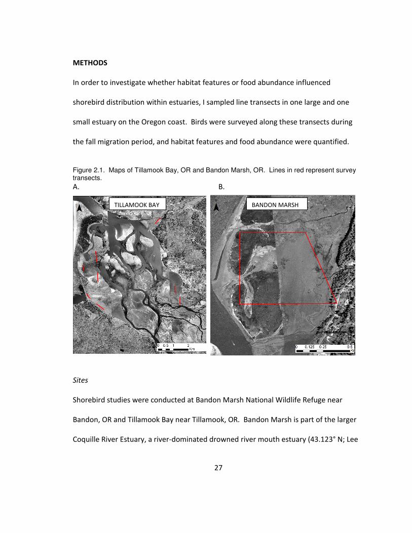
Figure 2.1. Maps of Tillamook Bay, OR and Bandon Marsh, OR. Lines in red represent survey transects.
A. B.
Sites
Shorebird studies were conducted at Bandon Marsh National Wildlife Refuge near
Bandon, OR and Tillamook Bay near Tillamook, OR. Bandon Marsh is part of the larger
Coquille River Estuary, a river-dominated drowned river mouth estuary (43.123° N; Lee
TILLAMOOK BAY BANDON MARSH

28
and Brown 2009). The intertidal zone (~0.5 km2) consists of sand and mudflats within a
matrix of low marsh that is located 1.75 km from the mouth of the larger estuary.
Tillamook Bay is a tide-dominated drowned river mouth estuary (45.513° N; Lee et al.
2009). It is one of the largest Oregon estuaries. The intertidal zones (25.6 km2) include
flats ranging from coarse sand to very fine silts. Some flats are bare while others include
seagrass and macro-algae beds.
Shorebird, prey, and habitat surveys were conducted from line transects (Figure
2.1). In Bandon Marsh, four line transects (range = 300-700 m in length) had been
previously established by refuge staff and roughly followed the edge of the major
mudflats. All mudflats had fairly similar elevation based on their flooding within ~30
minutes as the tide came in. In Tillamook, survey transects were randomly located
within four regions of the bay with good access points (northeast, NE (n = 1 transect;
200 m in length); southeast, SE (n = 2; 200-400 m); southwest, SW (n = 2; 200-400 m);
and west, W (n = 3; 200-400 m)). All eight Tillamook transects paralleled the shoreline.
In areas with relatively stable sediment, both the location along the shoreline and
distance from shore were randomly selected (n = 5 transects); in areas with unstable
sediment the location along the shoreline was randomly selected but the transect line
was placed along the shore (n = 3 transects). In Tillamook Bay, the survey area
boundary for each transect was separated by >100 m from neighboring survey area
boundaries. Based on inundation time, the SW region was relatively high elevation
while the NE region was low and the SW and W region were intermediate. While tidal

29
elevation was variable among regions, it tended to be similar within regions based on
the observation that when the tide came in it would cover a whole region very quickly.
Shorebird surveys
Shorebirds were surveyed every 7-10 days during the fall migration period from the end
of July to mid-September 2011. All surveys were started before noon. Six surveys were
completed in Tillamook and nine in Bandon. On each survey date, I or another trained
observer (1 observer per estuary) walked all of the transects at a given site during one
low tide period. For all shorebirds within 200 m of the transect line, the size of the flock,
species, and behavior (foraging, resting, flying) were recorded. We used 10x power
binoculars to identify and count birds and a laser range-finder to verify distances. The
specific location of the bird/flock was recorded (based on distance from and location
along the transect) and later mapped. Additionally, the general habitat type of the bird
or flock's location was recorded (mudflat, sandflat, seagrass bed, macroalgal bed, low
marsh or channel bed), including whether the bird was adjacent to the tidal edge. We
surveyed ahead with sufficient frequency to note locations of birds before they could be
disturbed. Given that a smaller proportion of Tillamook estuary was covered by these
transects, and that transects were relatively close to the shoreline, I also scanned larger
expanses of intertidal area with a spotting scope to qualitatively determine whether the
density of shorebirds along each transect was similar to that in the greater area of the
bay. In all cases, the density was similarly low in the surrounding flats.

30
Food resources and habitat measures
Infauna and biofilm were sampled systematically along all survey transects midway
through fall migration (Tillamook on 14 August 2011, Bandon on 18 August 2011). A
1m2 quadrat was placed every 100m along each transect at a random distance 0-100 m
from the transect. Infauna and biofilm samples were collected from within the quadrat.
The percent cover of seagrasses and macro-algae was estimated visually and the
approximate average size of sediment (coarse sand, fine sand, sand/mud, mud) was
estimated visually when sieved on a 500 µm screen.
For infauna, three 4 cm diameter cores were collected haphazardly within each
quadrat. Each core was split by depth: 0-3cm depth and 3-6cm depth samples. Three
centimeters corresponds to the maximum bill length of western sandpipers, while 6 cm
corresponds to the depth of larger billed shorebirds found in Oregon estuaries (e.g.,
Dowitcher spp). The upper sections of the three cores were combined as were the
three lower sections. Samples were sieved on a 500 µm screen, and then preserved in
10% buffered formalin. After 1-10 days, samples were transferred to 70% ethanol.
Infauna were sorted using a dissecting scope, identified to broad taxonomic groups, and
enumerated. Because less than 10% of organisms were in the lower half of the samples
and the majority of the birds observed had bills <3 cm, the analyses below were from
the upper three cm of the cores only.
Biofilm abundance was estimated by measuring Chlorophyll a and ash-free dry
mass of the surface sediment. The top 2mm of sediment were collected by placing an
31
inverted petri dish haphazardly within the quadrat (any macroflora were avoided). A
flat spatula was inserted underneath and the contents were rinsed into a sample bottle.
This was repeated three times within the quadrat and all of these sub-samples were
combined into one sample bottle. Sample bottles were promptly wrapped in tinfoil or
placed in an opaque bag to avoid light exposure. Samples were placed on ice and then
frozen upon return to the lab. Sub-samples were later taken for biofilm estimates.
Chlorophyll a was measured with a spectrometer and ash-free dry mass was measured
using loss-on-ignition methods; both measurements followed standard procedures
(APHA 1999).
Data Analysis and Statistics
In some cases, Western or Least sandpipers could not be distinguished so they were
grouped for analysis (hereafter referred to as "Small Sandpipers"). Because transects
differed in length between the estuaries, all data except for the raw number
shorebirds/survey and species composition data are presented as densities.
The study was designed to compare shorebird abundance to prey and habitat
features on a relatively broad within-estuary scale by comparing regions of the bay with
different habitat types to one another, and also to look at finer scale associations by
binning shorebird observations into 100 m x 100 m units. Because of the extremely low
number of shorebird observations in Tillamook Bay, this finer scale analysis was not
possible. Instead, comparisons were made using regions of the bay or individual

32
transects as the spatial unit. Groups of birds seen flying low to the ground (indicating
very local travel) were included in analysis of associations with food resources for
Tillamook only, because of the low sample size. I consider this valid because data were
grouped by region but not finer spatial scales. Only shorebirds on the ground were
included for Bandon.
Shorebird observations from Bandon Marsh were binned into 100 m2 bins for
subsequent analysis that related shorebird density to prey measures. Measurements of
food abundance were made within 100 m on one side of the transect whereas shorebird
observations were made to 200 m on either side of the transect. We used only the
shorebird observations within the 100 m band for shorebird vs food comparisons.
Binned shorebird observations, as well as prey measurements, were all tested for
autocorrelation using an autocorrelation function in order to ensure independence of
data points prior to proceeding with regression analyses.
Differences in food abundance between regions of the estuary were tested using
one-way ANOVAs. Differences in infaunal community composition among regions of the
estuary were evaluated with an NMDS ordination plot and Analysis of Similarity
(ANOSIM). The abundance of birds in relation to food resources was modeled using
negative binomial GLMs. The negative binomial was suitable because shorebird
abundance is count data and because it was highly over-dispersed (many zero values
and a few large values; the variance exceeded the mean). All analyses were conducted
with program R using library MASS for GLMs and library vegan for NMDS.
33
RESULTS
Overall shorebird abundance and composition
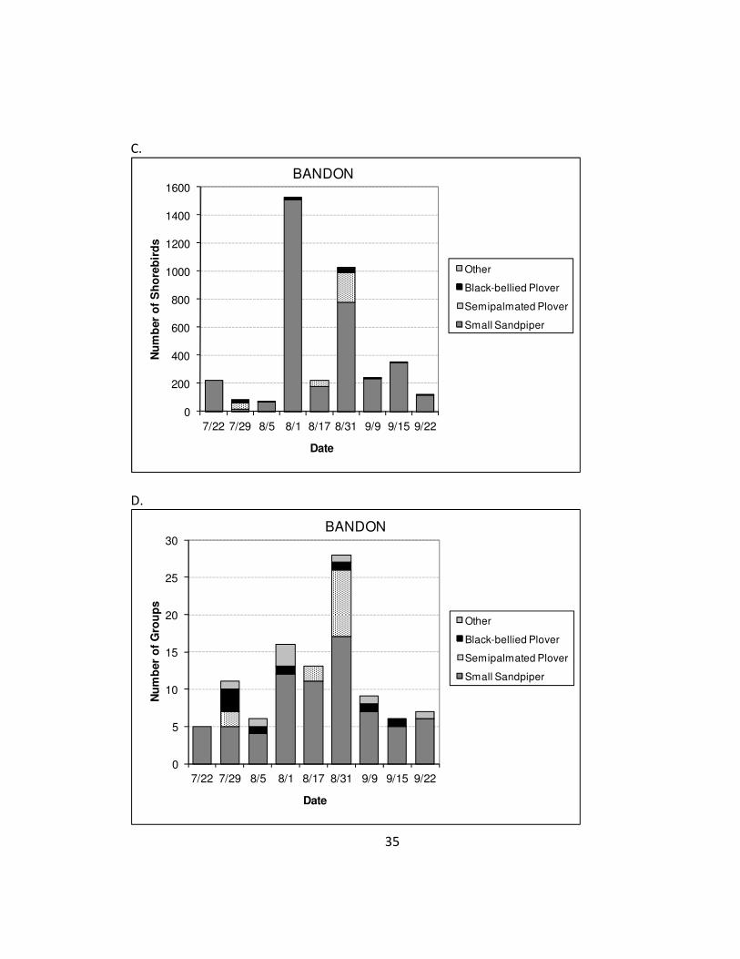
Observations during the six surveys in Tillamook ranged from 7- 472 birds in 1-6 groups
per survey (Figure 2.2a-b). Observations during the nine Bandon surveys ranged from
69-1,524 birds in 5-28 groups (Figure 2.2c-d). At Tillamook, 32% (±41% SD) of all
shorebirds were foraging; in Bandon 35% (±32% SD) were foraging. The majority of the
remaining birds were seen flying, or their behavior could not be determined.
Most shorebirds observed were Western or Least Sandpipers (Figure 2.2;
Bandon: 90.3%, Tillamook: 99.6%). Not all observations of small Sandpipers were made
to species level, but of those that were, 75% in Bandon and 100% in Tillamook were
Western Sandpipers; the remaining were Least Sandpipers. Semipalmated Plovers were
also observed regularly in Bandon (7.7%). Less than 2% of all observations were of other
species including Black-bellied Plovers, Black Turnstones, Greater Yellowlegs, Dunlin,
Dowitcher sp., and Red-necked Phalarope.

34
Figure 2.2. Number of shorebirds and number of flocks by species seen per survey in Tillamook Bay and Bandon Marsh, OR.
A.
0
200
400
600
800
1000
1200
1400
1600
7/27 8/12 8/13 8/17 8/28 9/12
Nu
mb
er
of
Sh
ore
bir
ds
Date
TILLAMOOK
Semipalmated Plover
Small Sandpiper
B.
0
5
10
15
20
25
30
7/27 8/12 8/13 8/17 8/28 9/12
Nu
mb
er
of
Gro
up
s
Date
TILLAMOOK
Semipalmated Plover
Small Sandpiper
35
C.
0
200
400
600
800
1000
1200
1400
1600
7/22 7/29 8/5 8/1 8/17 8/31 9/9 9/15 9/22
Nu
mb
er
of
Sh
ore
bir
ds
Date
BANDON
Other
Black-bellied Plover
Semipalmated Plover
Small Sandpiper
D.
0
5
10
15
20
25
30
7/22 7/29 8/5 8/1 8/17 8/31 9/9 9/15 9/22
Nu
mb
er
of
Gro
up
s
Date
BANDON
Other
Black-bellied Plover
Semipalmated Plover
Small Sandpiper

36
Patterns within Tillamook
The four regions of Tillamook Bay each had qualitatively distinct sediment and habitat
characteristics. The NE region primarily had silty sediment and had an average of 15%
cover of macroalgae. The SE region was dominated by large sand/cobble sediment and
20% cover of Zostera marina (with somewhat finer sediment in the seagrass beds). The
SW region had extremely fine silt sediments. There was 50% cover of seagrasses,
primarily Zostera japonica. The W region had sandy sediment, 12% cover of
macroalgae, and 9% cover of Z. marina based on the sampled quadrats.
Relatively small numbers of shorebirds were seen in Tillamook, and most of
those seen were flying. There were significant differences among regions of the bay in
both the number of flocks (Kruskal-Wallis X2
= 12.67, df = 3, p = 0.005) and the total
number of sandpipers (Kruskal-Wallis X2
= 12.63, df = 3, p = 0.006). Sandpipers were
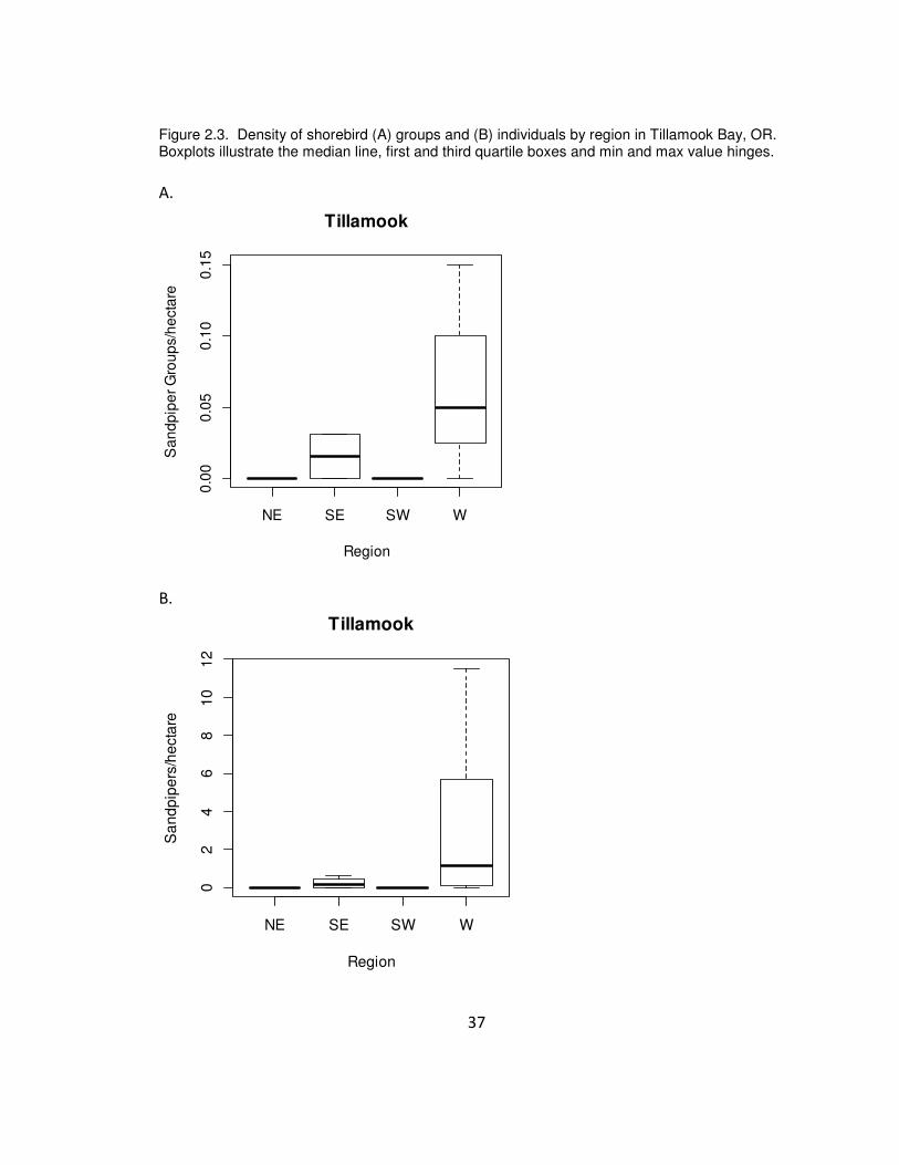
seen most frequently in the W region (Sandflats) and less frequently in the SE region
(Cobbleflats; Figure 2.3). No shorebirds were observed in the NE or SW regions, the
areas characterized by finer sediments.
37
Figure 2.3. Density of shorebird (A) groups and (B) individuals by region in Tillamook Bay, OR. Boxplots illustrate the median line, first and third quartile boxes and min and max value hinges.
A.
NE SE SW W
0.0
00
.05
0.1
00
.15
Tillamook
Region
Sa
nd
pip
er
Gro
up
s/h
ecta
re
B.
NE SE SW W
02
46
81
01
2
Tillamook
Region
Sa
nd
pip
ers
/he
cta
re

38
Figure 2.4. Infauna abundance and biofilm indicators, ash-free dry mass (AFDM) and chlorophyll a (CHLA), by region in Tillamook Bay, OR. Boxplots illustrate the median line, first and third quartile boxes and min and max value hinges with outliers excluded and shown as circles.
A.
NE SE SW W
01
00
30
05
00
Tillamook
Region
Infa
un
a (
Co
un
t)
B.
NE SE SW W
20
00
06
00
00
10
00
00
14
00
00
Tillamook
Region
AF
DM
(m
g/L
)

39
C.
NE SE SW W
50
00
10
00
01
50
00
Tillamook
Region
CH
LA
(m
cg
/L)
Infauna communities also varied with region, but abundance was not greatest in
the regions with the most sandpipers (Figure 2.4). Total abundance did not differ
significantly among regions (ANOVA: F3,23 = 0.73, p = 0.55). Certain taxonomic groups
were higher in particular regions, but variability tended to be high (Table 2.1).
Ordination indicated that the community of infauna in the West region was distinct
from that in the other regions (Figure 2.5; stress = .18; ANOSIM W-NE: R = 0.52, p =
0.003; ANOSIM W-SE: R = 0.37,p = 0.003; ANOSIM W-SW: R = 0.32, p = 0.2). The west
region had more bivalves and tanaids and fewer oligochaetes and cumaceans than the
other three regions in Tillamook Bay.
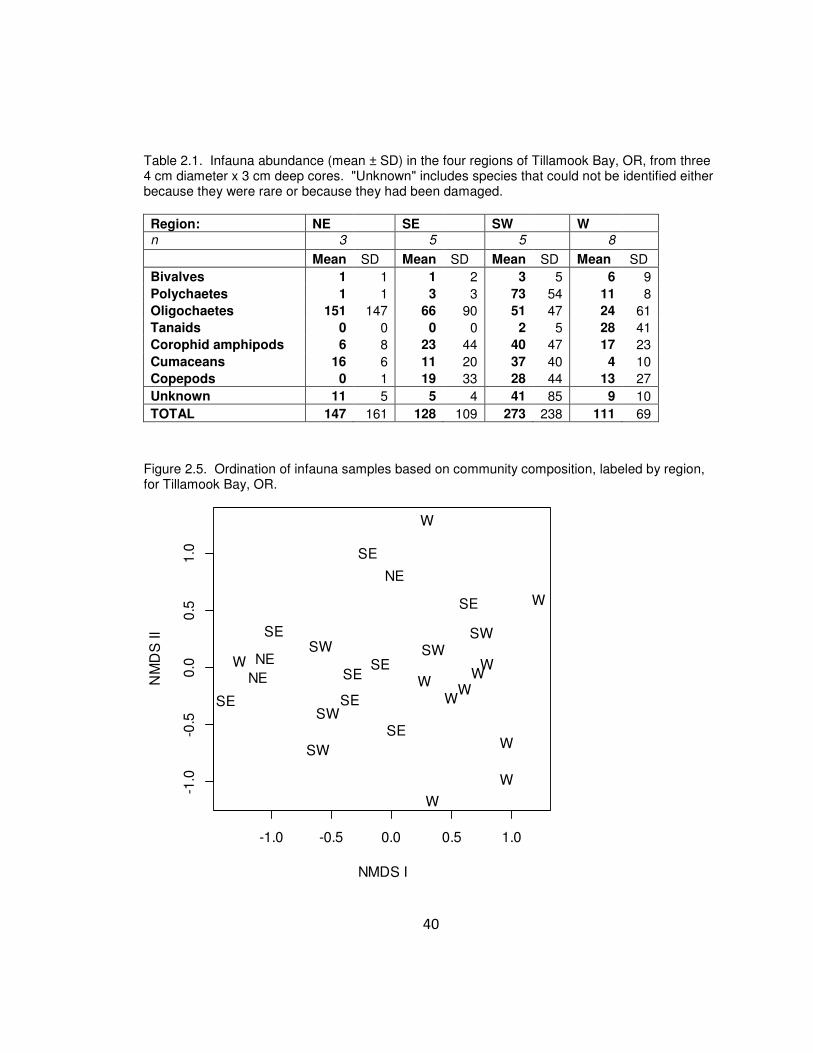
40
Table 2.1. Infauna abundance (mean ± SD) in the four regions of Tillamook Bay, OR, from three 4 cm diameter x 3 cm deep cores. "Unknown" includes species that could not be identified either because they were rare or because they had been damaged.
Region: NE SE SW W
n 3 5 5 8
Mean SD Mean SD Mean SD Mean SD
Bivalves 1 1 1 2 3 5 6 9
Polychaetes 1 1 3 3 73 54 11 8
Oligochaetes 151 147 66 90 51 47 24 61
Tanaids 0 0 0 0 2 5 28 41
Corophid amphipods 6 8 23 44 40 47 17 23
Cumaceans 16 6 11 20 37 40 4 10
Copepods 0 1 19 33 28 44 13 27
Unknown 11 5 5 4 41 85 9 10
TOTAL 147 161 128 109 273 238 111 69
Figure 2.5. Ordination of infauna samples based on community composition, labeled by region, for Tillamook Bay, OR.
-1.0 -0.5 0.0 0.5 1.0
-1.0
-0.5
0.0
0.5
1.0
NMDS I
NM
DS
II
W
W
W
W
NE
NE
NE
SE
SE SE
SE
SE
SE
SE
SE
SWSW
SW
SW
SW
W
W
WW
W
W
W

41
Biofilm indicators differed by region. Ash-free Dry Mass was significantly lower
in the West region, where the most shorebirds were seen, than in other regions (Figure
2.4b; ANOVA: F3,22 = 26.6, p < 0.001; Tukey-Kramer post-hoc tests for individual
comparisons). Chlorophyll a was lowest in the SE (Figure 2.4c; ANOVA: F3,22 = 10.3, p <
0.001). The other regions did not differ from one another for either AFDM or Chl A.
Sandpiper abundance was also compared to food abundance by transect. At the
scale of a transect, sandpiper abundance was negatively related to AFDM, although the
estimated effect was small. Sandpiper abundance was not correlated with overall
abundance of infauna or chlorophyll a (Table 2.2).
Table 2.2. Models of shorebird abundance in relation to infauna abundance and biofilm indicators, ash-free dry mass (AFDM) and chlorophyll a (CHLA) from surface sediment.
Negative Binomial GLMs: Estimate SE z-value p AIC
Infauna -0.02164 0.01266 -1.71 0.09 38.14
AFDM -7.18E-05 1.94E-05 -3.693 0.0002 34.13
CHLA -0.00022 0.000179 -1.226 0.22 45.38
Only five flocks of sandpipers were observed foraging during the surveys in Tillamook,
and all of these flocks were along the transect located furthest from shore in the West
region. All of these observations were also along channels or at the main edge of the
tide.

42
Patterns within Bandon Marsh
Overall, many more shorebirds were seen in Bandon Marsh on all surveys,
despite a smaller survey area. There was little variability within the survey region in
terms of our a priori habitat characterizations; therefore, we did not group our
observations by habitat or region as with Tillamook. Macroalgae and seagrasses
covered less than 25% of all sampling quadrats. All sediment in Bandon was
qualitatively similar in sediment composition, consisting of sandy-mud with many small
wood particles. Despite the relative homogeneity of sediment grain along the transects,
the habitat was not homogenous. Bandon Marsh has a large amount of marsh habitat
in the inter-tidal matrix, including along the transects (whereas there is no marsh
habitat in the Tillamook transects), as well as many small channels.
Shorebirds were observed on all of the transects, although there were relatively
few observations on the northern transect, which was dominated by marsh habitat.
Detection of shorebirds is more limited in the marsh environment; we observed only
one shorebird in the low marsh. However, our focus was on foraging birds and marsh
habitat is used primarily for roosting (Zharikov and Milton 2009). In general it appeared
that more observations occurred farther from the shore, and at several of the mouths
where the tide enters the mudflats.
Infauna were highly abundant but variable in Bandon Marsh. Corophid
amphipods dominated the infauna community (Table 2.3). Ash-free dry mass was
variable throughout Bandon Marsh (76,186 ±20,702; n=18); chlorophyll a was much

43
higher than in Tillamook samples and was highly variable among samples in Bandon
Marsh (38,821 ± 28,382, n=18).
Table 2.3. Infauna abundance (mean number of individuals ± SD) in Bandon Marsh, OR, from three 4cm diameter x 3 cm deep cores. "Unknown" includes species that could not be identified either because they were rare or because they had been damaged.
n=16 Mean SD
Bivalves 12 18
Polychaetes 67 47
Oligochaetes 68 47
Tanaids 0 0
Corophid Amphipods 411 525
Cumaceans 26 58
Copepods 17 20
Unknown 56 91
TOTAL 658 580
Autocorrelation plots showed no indication of spatial autocorrelation for birds or
for any of the food indicators, suggesting that bird and food abundances were
independent at the 1 hectare scale. Shorebird abundance was not correlated with
either infauna abundance or chlorophyll a, but did exhibit a very slight but positive
relationship with AFDM (Table 2.4; Figure 2.6). This relationship is driven by the fact
that the very largest flocks of shorebirds were observed in bins that also had high AFDM.
Table 2.4. Models of shorebird abundance in relation to infauna abundance and biofilm indicators, ash-free dry mass (AFDM) and chlorophyll a (CHLA) from surface sediment.
Negative Binomial GLMs: Estimate SE z-value p AIC
Infauna -0.00022 0.0018 -0.117 0.91 123.4
AFDM 8.66E-05 3.49E-05 2.48 0.013 122.1
CHLA -3.28E-05 4.36E-05 -0.752 0.45 126.0

44
Figure 2.6. Infauna abundance and biofilm indicators, ash-free dry mass (AFDM) and chlorophyll a (CHLA), in relationship to shorebird abundance per hectare plot in Bandon Marsh, OR.
A.
500 1000 1500
01
00
20
03
00
40
05
00
Infauana (count)
Sm
all S
an
dp
ipe
rs (
co
un
t)
B.
10.9 11.0 11.1 11.2 11.3 11.4 11.5
01
23
45
6
AFDM (mg/L)
Sm
all S
an
dp
ipe
rs (
co
un
t)

45
C.
20000 40000 60000 80000
01
00
20
03
00
40
05
00
CHLA (mcg/L)
Sm
all S
an
dp
ipe
rs (
co
un
t)
Although channels occupied only a small proportion of the total survey area,
41% of all flocks of sandpipers and 51% of the total numbers of shorebirds were
observed in or immediately adjacent to channels. A higher percent of sandpipers were
foraging when observed next to a channel (73%) than when observed in open mudflats
(60%; Pearson's X2
= 50.296, df = 1, p < 0.001).
DISCUSSION
In Tillamook Bay, shorebirds had a non-uniform distribution with most observations
along a single transect in the Western region, supporting my first hypothesis that
46
shorebirds would have non-random distributions within estuaries. In Bandon Marsh
shorebirds also appeared to have a non-random distribution; however, there was too
much variability in shorebird locations among observation dates to identify specific
targeted areas.
The hypothesis that shorebirds would be more abundant where there was
moderate to high density of food within each estuary was not supported. Shorebirds in
Tillamook were found primarily in a region with lower infauna abundance and lower
measures of biofilm than the other regions. Analysis at the scale of individual transects
also did not show any relationship between shorebirds and infauna or Chl A, and there
was a negative relation to AFDM. It is unlikely that sandpipers actively avoided areas
with high surface organic content; rather, shorebirds may have favored the region of
lower AFDM for independent reasons. Shorebird distribution in Bandon Marsh,
measured at a finer scale, also did not correlate to infauna abundance or Chl A. A
positive relationship existed between shorebird abundance and AFDM. However, this
relationship was quite weak and driven largely by several data-points: the three bins
where the most birds were observed had high AFDM but there were many other
locations with high AFDM where birds were not frequently observed. The fact that a
negative relationship was detected in Tillamook but a positive relationship was detected
in Bandon further suggests that this is not a consistent pattern and may be spurious.
In Bandon Marsh, we may not have seen a numerical response to infauna
density in part because prey density was so high. Bandon Marsh samples contained an

47
average of 658 (± 580, n = 16) invertebrates, whereas Tillamook had 165 (± 150, n = 21)
on average. The density of infauna at Tillamook was comparable to estimates made by
other researchers at Tillamook and at Gray's Harbor and Willapa Bay (Ferraro and Cole
2011, 2012; see Chapter 1 for details). Therefore, the density of prey may be several
times higher at Bandon Marsh than other Pacific Northwest Estuaries. Numerical
responses are often non-linear. It is plausible that no numerical response to prey was
observed in Bandon because infauna abundance was high enough to exceed the plateau
of an asymptotic numerical response (Type II or Type III; Holling 1959).
I measured prey abundance as all infauna that did not pass through a 500 μm
sieve; however, shorebirds may select for certain prey species either because of a
difference in nutritional content or a difference in behavior that leads to easier capture
and handling. The Western region of Tillamook Bay, where most shorebirds were
observed, did differ from other regions in infauna community composition. It had
greater relative abundances of bivalves and tanaids. It is plausible that these were
preferable prey items, although there has been no specific research on sandpiper prey
selection in this region. Infauna at Bandon Marsh was dominated by Corophium sp
amphipods. Corophium are known to be the primary prey item for Semipalmated
Sandpipers in the Bay of Fundy, Canada (Wilson 1990) as well as for small sandpipers in
Northern California (Colwell 1993, Colwell and Landrum 1993). Alternatively to
shorebirds selecting prey, certain prey may be more available because of their depth
48
relative to the depth a bird can probe, or because of some other difference such as their
activity pattern. I did not measure availability per se in this study.
Sandpipers in Tillamook were found most often in the sand-flat region and never
in the muddiest region. Lamberson et al. (2011) investigated shorebird distribution
within Yaquina Bay, Oregon over one year. They found that shorebirds used sandflats
more frequently than other habitat types overall, although mudflats were used more
often than sandflats during the fall and spring migration periods. However, region
within an estuary predicted abundance better, controlling for habitat types. Taken
together with our results, it appears that shorebirds in Oregon forage primarily in open
mud and sandflats, but also may select regions of estuaries independently of sediment
grain. Sediment at Bandon Marsh was too uniform to make a comparison of habitats.
At both sites foraging sandpipers were frequently found along channels. Micro-
habitat features such as the tidal edge, channels, or ponds have previously been found
to be predictors of shorebird abundance (Colwell and Landrum 1993, Yates et al. 1993,
Warnock and Takekawa 1995, Danufsky and Colwell 2003, Finn et al. 2008, Lamberson
et al. 2011) either due to elevated prey abundance or availability. Because channels
remain inundated for longer times during the tide cycle, the wetter sediments may
increase prey abundance or availability. I investigate this pattern with more detailed
observations in Chapter 3.
Factors other than food abundance and availability may be more important
drivers of shorebird distribution in these estuaries. Shorebirds are often attacked by
49
falcons at estuaries. Dekker and Ydenberg (2004) demonstrated that Dunlin in British
Columbia were killed more frequently when they foraged close to shore. Pomeroy
(2006) found that Western Sandpipers in the same region trade-off proximity to
shoreline versus infauna abundance in choosing foraging locations. Therefore, being
further from shore, where predators may more easily hide, may be of significant
importance, particularly when the density of other shorebirds is low. The transect
where the most shorebirds were observed in Tillamook was the furthest from shore.
The influence of predation may be particularly important in smaller estuaries where
there is a greater edge effect. If shorebirds habitat use reflects avoidance of either
predators or areas with human activity, these effects may limit how much of the estuary
they are able to use and supersede the influence of local prey distribution. Future work
in Oregon should investigate predation risk and human disturbance and how these
impact shorebird distributions and abundance.
Proximity to marsh habitat and other potential roost sites may also be an
important factor determining shorebird distribution within estuaries. Preferred roost
sites are typically closer to large foraging areas (Zharikov and Milton 2009). Although
Tillamook Bay is much larger than Bandon Marsh, both are small compared to the major
West Coast estuaries. In smaller estuaries, flight costs to a specific roost site are
minimized but should still be considered, particularly since marsh and grasslands were
both factors I identified in Chapter 1 as being positively correlated with shorebird
density among estuaries.
50
Spatial and temporal scales are important to consider when evaluating shorebird
associations with prey and habitat. In comparing food abundance among estuaries in
Chapter 1, I showed a general trend of increasing shorebird density with food density in
the fall although the total number of sites was limited. The relationship to food
resources may be stronger when comparing estuaries to one another rather than
movement within an estuary. Mismatches in scales of measurement in this study could
also explain the lack of correlation between shorebirds and food resources. Shorebirds
were surveyed over several months and the survey area was large relative to the
number of food resource samples. If infauna or biofilm were highly patchy, the samples
we collected may not have adequately reflected the broader areas they represented. If
this is the case, then a numerical response might be detected at a finer scale. I describe
more detailed study of shorebird movements within estuaries in Chapter 3 in relation to
channels and associated prey resources.

51
Chapter 3. Small tidal channels improve foraging opportunities for Calidris shorebirds
INTRODUCTION
Migration is energetically demanding, so many shorebird populations stop to rest and
forage in the mudflats of estuaries. Estuarine inter-tidal microhabitats are non-uniform
and both abiotic and biotic factors may serve as predictors of whether migratory
shorebirds will use a given site. Microhabitat characteristics such as the sediment size,
elevation, salinity, and hydrodynamics can directly alter the prey community (Lenihan
and Micheli 2001) as well as the availability of prey to foraging birds and, therefore,
indirectly relate to shorebird abundance. These features may therefore be useful as
indicators of potential foraging opportunities for shorebirds.
At-risk populations of the Western Sandpiper Calidris mauri and the Dunlin C.
alpina pacifica use estuaries in the Pacific Northwest as stop-over sites during their
migrations. Wildlife managers and land managers are seeking ways to improve the
quality as well as quantity of foraging grounds for these and other declining shorebird
populations. In this chapter I investigate how a common microhabitat feature, small
tidal channels in mudflats, influences foraging shorebirds.
Shorebirds often follow the main tidal edge as the tide ebbs and flows (Recher
1966, Colwell and Landrum 1993, Finn et al. 2008), possibly because the shorebirds'
prey may be found closer to the surface after recent exposure when they are at lower
risk of desiccation. Alternatively, the sediment may be easier to probe when it is still

52
relatively water logged. Kuwae et al.’s (2010) observation that Dunlin switched from
probing in the sediment to pecking at the surface after a longer period of mudflat
exposure is consistent with either hypothesis.
Channels in mudflats may offer similar advantages to foraging shorebirds, either
in terms of the depth of their prey or the penetrability of the sediment, because they
create similar physical conditions to the tidal edge. Channels and other similar water
features have been found to be positively associated with Western Sandpiper or Dunlin
presence or density in several studies in Western Europe or the west coast of the U.S.
However, the effects were weak and/or statistically insignificant (Ravenscroft and
Beardall 2003, Danufsky and Colwell 2003, Warnock and Takekawa 1995). One study
more thoroughly investigated shorebird associations with tidal channels. Lourenco et al.
(2005) examined wintering shorebird populations in Portugal and showed that
shorebirds, including Dunlin, foraged more often near channels. They attributed this to
the greater abundance of prey found in the sediment near the channels. Therefore,
channels may confer another advantage – prey density – beyond that conferred by the
tidal edge. However, this pattern has not been examined at other stop-over sites or for
other shorebird species. Furthermore, the differences along channels in prey
abundance, depth and accessibility (in terms of how soft sediment is) have not been
evaluated together to understand their relative importance.
The first objective of my research was to determine whether shorebirds
preferentially fed near tidal channels and tidal edge in Bandon Marsh National Wildlife

53
Refuge, a primary stop-over site in Oregon. By surveying foraging shorebirds at sites
adjacent to and distant from channels at different times of the tide cycle, I tested two
hypotheses: (H1) Calidris shorebirds forage more often and probe deeper in the
sediment along the edges of channels, and (H2) Calidris shorebirds forage along
channels more often later in the cycle of tidal exposure (at low and flow tides as
compared to ebb tides).
My second objective was to determine what characteristics differentiate the
quality of foraging along channels. I tested three non-exclusive hypotheses about
channels that are consistent with improved foraging efficiency for Calidris shorebirds. I
hypothesized that foraging would be improved along channels because (H3) infauna are
more abundant, (H4) prey is closer to the surface throughout tidal exposure, and (H5)
the sediment is softer and easier to probe throughout tidal exposure.
To test these hypotheses, I collected samples of prey at set distances from a
channel during ebb and low tides and separated these samples by sediment depth. I
also measured the force required to probe in the sediment at these locations. Herein, I
evaluate the relative merit of these three hypotheses.
Methods
Research Site
Evaluation of the value of channel habitat to shorebirds was conducted at Bandon
Marsh National Wildlife Refuge in Bandon, OR. Bandon Marsh hosts one of the highest
54
densities of migratory shorebirds in Oregon (PRBO unpublished data, chapter 1).
Bandon Marsh is located in the Coquille River Estuary and is on a side channel of the
river. The site is approx 0.5 km2 of mudflat surrounded by low and high marsh zones.
Several major channels and many smaller channels meander through parts of the
mudflats. Research focused on the NW corner of the marsh where several channels
flow through the mudflat.
Shorebird Surveys
Shorebird surveys were conducted daily from 25 April to 1 May between mid-ebb and
mid-flow tides. I scanned the entire NW region of Bandon Marsh when the tide was at
0.91 m, just after the majority of the mudflats became exposed, then again at 0.61 m,
0.30 m, 0 m, low tide (if lower than 0 m) and at the same tidal heights during tidal flow.
The time between the scans ranged from 45-75 min apart. For each flock of shorebirds,
I recorded the species, size of flock, distance from channel edge (0-5m, >5m), and
behavior (foraging, roosting, etc.). I also recorded the microhabitat as either Flats (open
flats; total of 38,089 m2), sandy beach (sandy flats along the Coquille River beach;
29,460 m2), Red Algae (sandy-mudflat covered >50% with Gracilaria sp; 3,475 m
2),
Green Algae (sandy-mudflat covered >50% with dense green algal mat; 9,744 m2), or
channel (within 1 m of a channel or exposed channel bed; 8,790 m2).
I conducted focal observations during the same dates to assess individual
foraging behaviors and allocation of time to different behaviors at channel and non-
55
channel sites. I selected shorebird flocks opportunistically, and then selected an
individual bird within the flock haphazardly and blindly. Observations lasted ~1 min
unless the bird was lost from the field of view. I recorded the number of pecks and
probes into a handheld digital voice recorder. I also recorded the percentage of time
spent foraging or in other behaviors (e.g., running or other movement, predator
vigilance, preening).
Quantifying Quality of Channel Sites
The abundance and depth of infauna, as well as the penetrability of the sediment, were
measured at sites along channels and away from channels at different tide heights.
Eight sites were randomly selected along channels in the area of observation. At each
site, a 4 cm diameter core of infauna was collected immediately adjacent to the channel
(within 0.1 m of the channel water edge) and at 5 m distance away from the channel to
determine differences in prey abundance. The distance of 5 m was selected following
the findings of Lourenco et al. (2007) that infauna community differences could be
detected at this distance, yet 5 m was close enough to minimize physical differences
other than the presence of the channel itself. To determine differences in prey depth,
each core was split by depth strata: surface-0.5 cm, 0.5-1.5 cm, and 1.5-3 cm (maximum
length of a Western Sandpiper bill is 3 cm but most are shorter, Wilson 1994; Dunlin bill
length can exceed 3 cm but Mouritsen and Jensen 1992 measured 3.5 cm as maximum
probing depth). To understand how these factors interact with tidal height, samples

56
were collected at mid-ebb tide (2’) and at low tide (0’). Infauna samples were later
sieved at 500 µm, preserved in formalin and then transferred to ethanol. Individual
infauna were enumerated and identified to major taxonomic group. Larger infauna
were also counted separately (>2 mm for amphipods, >5 mm for polychaetes). One
trained observer measured these organisms initially and then visually placed them into a
size category. Sediment penetrability was measured adjacent to each core location and
time with a soil penetrometer. Any seagrass or algal cover was noted.
Because shorebirds were often found in areas covered in red algae (Gracilaria
sp.), additional infauna samples (n = 5) were taken in this habitat. All sites in the red
algae habitat were at least 5 m from a channel. The paired channel and non-channel
sites were not in the Gracilaria.
Analysis
Differences in the relative density of shorebird flocks and individuals were tested using
ANOVA and Tukey Kramer post hoc tests. A percentage was used as opposed to raw
counts because there was high variability among days in the numbers of birds observed.
The percentage of all the birds or flocks seen in one day in a given habitat was divided
by the area of that habitat to give relative density. Data were log transformed to meet
normality assumptions. Logistic regression was used to evaluate whether the likelihood
of foraging along a channel changed with tidal height. A t-test was used to test the

57
difference in percentage probes (the number of probes divided by the total number of
pecks and probes) between channel and non-channel habitats.
Differences in infauna abundance in relation to sediment depth, distance from
channel, and difference from tide height were tested using multi-factor ANOVA models.
Because depth stratifications differed in total volume, infauna numbers were adjusted
to number per 0.5 cm depth for statistical tests. First and second-order interactions
were considered and non-significant interaction terms were removed. Both total
infauna abundance and abundance of Corophium amphipods were tested. A multi-
factor ANOVA was also used to test the difference in force required to probe in
sediment. Further, paired one-tailed t-tests were used to compare differences between
ebb and low tide. All analysis was performed in R (v. 2.8.1; R Development Core Team
2008).
RESULTS
Shorebirds
Western Sandpipers and Dunlin foraged most often, relative to total area, in the
sections of Bandon Marsh covered with red algae (Gracilaria sp.), followed by channel
beds (Figure 3.1). Many fewer of both species were observed foraging in the green
algae, open flat or sandy beach habitats. The differences among habitats were
significant for Western Sandpiper flocks (F4,30 = 103.71, p < 0.001), Western Sandpiper
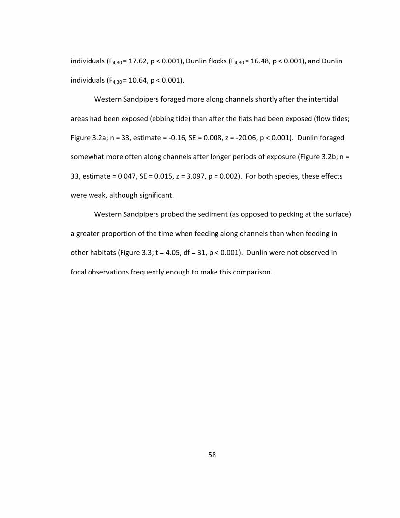
58
individuals (F4,30 = 17.62, p < 0.001), Dunlin flocks (F4,30 = 16.48, p < 0.001), and Dunlin
individuals (F4,30 = 10.64, p < 0.001).
Western Sandpipers foraged more along channels shortly after the intertidal
areas had been exposed (ebbing tide) than after the flats had been exposed (flow tides;
Figure 3.2a; n = 33, estimate = -0.16, SE = 0.008, z = -20.06, p < 0.001). Dunlin foraged
somewhat more often along channels after longer periods of exposure (Figure 3.2b; n =
33, estimate = 0.047, SE = 0.015, z = 3.097, p = 0.002). For both species, these effects
were weak, although significant.
Western Sandpipers probed the sediment (as opposed to pecking at the surface)
a greater proportion of the time when feeding along channels than when feeding in
other habitats (Figure 3.3; t = 4.05, df = 31, p < 0.001). Dunlin were not observed in
focal observations frequently enough to make this comparison.

59
Figure 3.1. Relative density (percent per m2) of (a) Western Sandpiper flocks, (b) Western
Sandpiper individuals, (c) Dunlin flocks, and (d) Dunlin individuals by habitat type. and log transformed. Letters indicate habitat types that differed significantly based on post-hoc tests. N=7 observation dates. Boxplot illustrates the median line, first and third quartile boxes and min and max value hinges with outliers excluded and shown as circles.
A.
Channel Flats Green Algae Red Algae Sand Beach
0.0
0.1
0.2
0.3
0.4
0.5
Habitat
ln W
este
rn S
andpip
er flocks (%
/m^2)
B.
Channel Flats Green Algae Red Algae Sand Beach
0.0
0.2
0.4
0.6
0.8
1.0
Habitat
ln W
este
rn S
andpip
ers
(%
/m^2)
B C BC A C
B D C A D

60
C.
Channel Flats Green Algae Red Algae Sand Beach
0.0
0.2
0.4
0.6
0.8
1.0
1.2
1.4
Habitat
ln D
unlin flo
cks (%
/m^2)
D.
Channel Flats Green Algae Red Algae Sand Beach
0.0
0.5
1.0
1.5
2.0
Habitat
ln D
unlin (%
/m^2)
A B B A B
AB BC BC A C
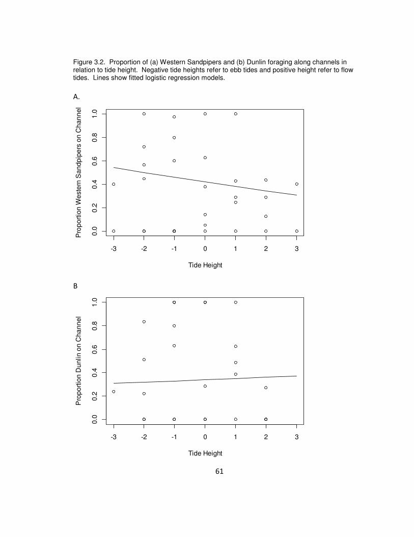
61
Figure 3.2. Proportion of (a) Western Sandpipers and (b) Dunlin foraging along channels in relation to tide height. Negative tide heights refer to ebb tides and positive height refer to flow tides. Lines show fitted logistic regression models.
A.
-3 -2 -1 0 1 2 3
0.0
0.2
0.4
0.6
0.8
1.0
Tide Height
Pro
port
ion
We
ste
rn S
an
dpip
ers
on C
han
nel
B
-3 -2 -1 0 1 2 3
0.0
0.2
0.4
0.6
0.8
1.0
Tide Height
Pro
port
ion
Du
nlin o
n C
ha
nn
el
62
Figure 3.3. Proportion of Western Sandpiper foraging actions that were probes (as opposed to pecks at the surface) along channels or in other habitats (red algae habitat excluded). Boxplot illustrates the median line, first and third quartile boxes and min and max value hinges with outliers excluded and shown as circles.
Channel Other
0.0
0.2
0.4
0.6
0.8
1.0
We
ste
rn S
an
dp
ipe
r %
Pro
be
s
Infauna
Total infauna abundance and large infauna abundance varied significantly with depth
and distance from the channel, but not with tidal stage (Table 3.1). Most infauna were
found in the top 0.5 cm of the sediment in all samples regardless of distance from
channel or tide height (Figure 3.4a). Infauna abundance was over twice as high, on
average, immediately adjacent to the channel as it was 5 m away from the channel. This
was true regardless of tidal height. There was a greater proportion of total infauna in
the top 0.5 cm at channel versus non-channel sites (Figure 3.4a), explaining the
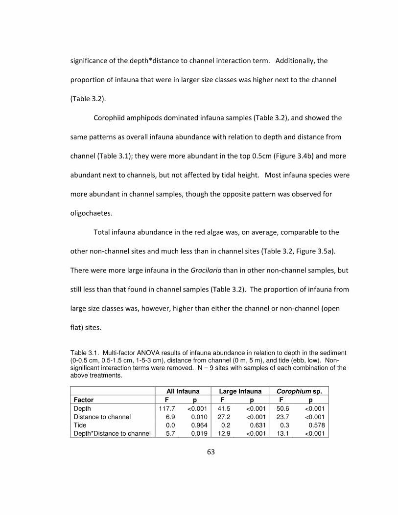
63
significance of the depth*distance to channel interaction term. Additionally, the
proportion of infauna that were in larger size classes was higher next to the channel
(Table 3.2).
Corophiid amphipods dominated infauna samples (Table 3.2), and showed the
same patterns as overall infauna abundance with relation to depth and distance from
channel (Table 3.1); they were more abundant in the top 0.5cm (Figure 3.4b) and more
abundant next to channels, but not affected by tidal height. Most infauna species were
more abundant in channel samples, though the opposite pattern was observed for
oligochaetes.
Total infauna abundance in the red algae was, on average, comparable to the
other non-channel sites and much less than in channel sites (Table 3.2, Figure 3.5a).
There were more large infauna in the Gracilaria than in other non-channel samples, but
still less than that found in channel samples (Table 3.2). The proportion of infauna from
large size classes was, however, higher than either the channel or non-channel (open
flat) sites.
Table 3.1. Multi-factor ANOVA results of infauna abundance in relation to depth in the sediment (0-0.5 cm, 0.5-1.5 cm, 1-5-3 cm), distance from channel (0 m, 5 m), and tide (ebb, low). Non-significant interaction terms were removed. N = 9 sites with samples of each combination of the above treatments.
All Infauna Large Infauna Corophium sp.
Factor F p F p F p
Depth 117.7 <0.001 41.5 <0.001 50.6 <0.001
Distance to channel 6.9 0.010 27.2 <0.001 23.7 <0.001
Tide 0.0 0.964 0.2 0.631 0.3 0.578
Depth*Distance to channel 5.7 0.019 12.9 <0.001 13.1 <0.001
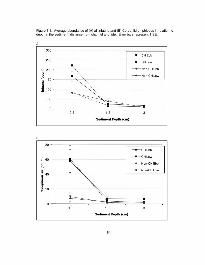
64
Figure 3.4. Average abundance of (A) all infauna and (B) Corophiid amphipods in relation to depth in the sediment, distance from channel and tide. Error bars represent 1 SE.
A.
0
50
100
150
200
250
300
0.5 1.5 3
Infa
un
a (
co
un
t)
Sediment Depth (cm)
CH Ebb
CH Low
Non-CH Ebb
Non-CH Low
B.
0
20
40
60
80
0.5 1.5 3
Co
rop
hiu
m s
p.
(co
un
t)
Sediment Depth (cm)
CH Ebb
CH Low
Non-CH Ebb
Non-CH Low

65
Table 3.2. Total abundance of infauna (mean ± SD) in paired Channel and Non-channel sites, and in Gracilaria habitat. Large infauna includes amphipods >2 mm and polychaetes >5 mm.
Channel Non-channel Red Algae
n = 16 n = 16 n = 5
Mean SD Mean SD Mean SD
Bivalves 7.2 ± 7.2 2.5 ± 2.4 3.4 ± 1.3
Polychaetes 5.4 ± 7.2 4.5 ± 3.5 6.0 ± 1.9
Oligochaetes 39.3 ± 28.7 67.4 ± 51.7 36.8 ± 9
Corophid Amphipods 68.6 ± 58 11.9 ± 19.2 26.8 ± 15.1
Gammarid Amphipods 7.9 ± 20.1 0.1 ± 0.3 5.6 ± 3.8
Cumaceans 3.7 ± 3.7 0.8 ± 1.5 0.6 ± 0.9
Copepods 89.9 ± 98.3 28.9 ± 31 15.8 ± 9.7
TOTAL INFAUNA 228.6 ± 134.1 118.2 ± 52 100.8 ± 26.6
% LARGE INFAUNA 11.7% ± 6.8% 4.8% ± 3.6% 16.0% ± 3.5%
Sediment Penetrability
Less force was required to probe in sediment next to channels than away from channels
(Figure 3.5b). A multi-factor ANOVA showed that this distance from channel was
significant (F = 24.82, p < 0.001), but that there was no difference in force with tide
height (F = 1.60, p = 0.21). The interaction term was not significant and was removed
from the model. However, paired t-tests showed that non-channel sites required more
force to probe at low than ebb tides (t = -6.057, df = 19, one-tailed p < 0.001) but
channel sites did not differ between ebb and low tides (t = -2.042, df = 9, one-tailed p =
0.36).

66
Figure 3.5. Average (A) abundance of infauna for all depths combined and (B) force required to probe in the sediment. Channel and other habitats were from paired samples taken 5 m apart; random samples were collected separately for the red algae microhabitat. Error bars show 1 SD.
A.
0
50
100
150
200
250
300
350
400
450
Channel Channel Other Other Red Algae Red Algae
Ebb Low Ebb Low Ebb Low
Infa
un
a (
avera
ge c
ou
nt)
B.
0
0.1
0.2
0.3
0.4
0.5
CH CH Non-CH Non-CH
Ebb Low Ebb Low
Fo
rce (
kg
/cm
2)

67
DISCUSSION
Western Sandpipers and Dunlin both foraged relatively more often along small tidal
channels than in most other habitat types in Bandon Marsh as I had predicted
(Hypothesis 1). Several previous studies of Western Sandpiper habitat use on the west
coast of North America have suggested a positive association with channelization
(Danufsky and Colwell 2003, Warnock and Takekawa 2005), although the first of these
was not supported with statistical validation and the second could not clearly distinguish
between the value of tidal sloughs and open mudflat. Lourenco et al. (2007) found that
Dunlin wintering in a Portuguese estuary were more likely to forage along channels, and
Ravenscroft and Beardall (2003) found a similar but non-significant pattern in estuaries
in the United Kingdom, observing that variability in numbers was high. Danufsky and
Colwell (2003) found no association between Dunlin presence or density and
channelization in Humboldt Bay although they made observations over a broader spatial
scale. Taken together, this literature suggests channels are commonly used by both
Western Sandpipers and Dunlin, but detecting this trend can be difficult because of the
frequent movement of flocks or because habitat selection occurs on a finer spatial scale.
Infauna were about twice as abundant next to channels compared to open flats.
This pattern was true for corophiid and gammarid amphipods, bivalves, copepods and
cumaceans. Oligochaetes were the only taxon to exhibit greater abundance further
from the channel. Similarly, Lourenco et al. (2005) also showed greater abundances of
bivalves, polychaetes, and a gastropod along channels in Portugal. These parallel results

68
in different parts of the world suggest that this is not just a local effect; channels are
likely to be advantageous to shorebirds world-wide.
Most infauna (> 90%) were found in the top 0.5 cm of sediment regardless of the
location. The proportion of total infauna in this top layer was greatest alongside
channels. However, the depth stratification of infauna did not change with the tide
height. Taken together with total infauna abundance, these patterns indicate that
shorebirds forage along channels primarily because prey is abundant (Hypothesis 3). The
decrease in prey depth next to channels is likely a secondary advantage (Hypothesis 4).
In addition to increased infauna abundance, channels may have attracted
foraging shorebirds because the sediment required less force to probe as measured
with the penetrometer. Furthermore, focal observations showed that Western
Sandpipers used more probing behaviors next to channels than in open flats. In
previous studies Dunlin were shown to probe more when sediment is water-logged
(Mouritsen and Jensen 1992, Kuwae et al. 2010). Mouritsen and Jensen (1992)
estimated with a simple model that Dunlin foraging success would increase up to 4-fold
with increased ability to probe because of an increased probability of encounter with
prey. I was not able to consistently determine whether a peck or probe was successful,
but I did often see large polychaete worms captured when a shorebird was probing, but
never saw such large infauna when the birds pecked.
Estuarine infauna are able to tolerate varying amounts of desiccation when the
tide is out (Lenihan and Micheli 2001); however, they may also avoid desiccation by

69
burrowing deeper in the sediment. I therefore expected that channels might be
particularly important to shorebirds later in the tide cycle because the sediment would
retain moisture and the prey would be more likely to remain near the top of the
sediment than in the open flats. I did not detect differences in infauna abundance or
depth between ebb and low tides. My sampling approach may not have effectively
detected these differences because infauna near the surface may have always burrowed
deeper due to the activity we created when sampling. However, the hypothesis that
shorebirds would forage more along channels during low tide (H2) was not supported
either; shorebirds appeared to use channels approximately equally throughout the tide
cycle, and infauna tended to be in the top-most substrate regardless of the time in the
tide cycle. Given that total infauna abundance was so much higher along channels, it is
likely that shorebirds were attracted to these locations at all times, and therefore would
have showed no change in distribution even if the depth of infauna were changing
somewhat.
This research was conducted at a generally cool and rainy location, which also
may have affected infauna depth patterns. On most days of survey, there was some
rain, and I observed a noticeable slick of water over the mudflats on these days even
late in the tide cycle. There was only one continuously sunny day of observation, and on
that day both Western Sandpipers and Dunlin used the channel in much greater
proportions during flow tide (75%) than ebb (25%). This anecdotal observation suggests
that in more southern locations the timing of the tide may have a greater impact on

70
infauna depth. Shorebird prey have been shown to be found deeper in the sediment at
more southern or sunnier wintering locations (Mathot et al. 2007). Further
investigation could determine whether depth stratification in these locations is affected
by proximity to channels and how this affects shorebird movement during the tide cycle.
Although small tidal channels were generally used more than other habitats, the
relatively small patches of Gracilaria in the mudflats attracted even greater densities of
shorebirds. Infauna in the Gracilaria patches was not, surprisingly, any greater than in
other areas of the open flats. Although total infauna abundance was not higher, I did
observe when collecting the samples that a fair number of large invertebrates were
inhabiting the algae itself. Although some Gracilaria was in each core we collected, we
may not have effectively captured the infauna residing in it. Furthermore, whether
more abundant or not, it may be easier for Western Sandpipers and Dunlin to capture
invertebrates in this filamentous algae compared to probing in the sediment.
Additionally, I noted that the Gracilaria patches retained small puddles of water.
Although the sediment was not softer than along channels, it was softer than the open
flats. Furthermore, if the retained water led to increased invertebrate activity, this
could assist foraging shorebirds. Finally, I also noted that shorebirds were well
camouflaged when in the Gracilaria so this environment could potentially reduce their
predation risk.

71
Conclusions
In this research, I demonstrated that Western Sandpipers and Dunlin preferentially
forage along channels in Bandon Marsh. This is the first such evidence for Western
Sandpipers, and the first for the Dunlin subspecies C. alpina pacifica. Furthermore, I
demonstrated why channels may be advantageous: infauna are more abundant,
including an important prey item Corophium sp.; infauna are more likely to be near the
surface, and the sediment is easier to probe. Based on the magnitude of variation, it
appears that total infauna abundance and ease of probing are likely to be of primary
importance while the difference in infauna depth stratification is secondary. Because
channelization in an estuary can be influenced by management actions, either directly in
restoration or indirectly in controlling sediment or freshwater run-off, these findings can
be used to improve site quality in stop-over sites for these at-risk shorebird species.

72
Conclusions
My goal in this research was to identify environmental features or habitat
characteristics that predict shorebird abundance in Oregon estuaries. Given the
dependency of sensitive shorebird species on estuaries, increasing our knowledge about
their habitat or prey needs can help wildlife managers increase both the amount and
the quality of shorebird habitat.
On a large spatial-scale, comparing estuaries throughout the Pacific Northwest, I
showed that shorebird density in the spring was best predicted by total size rather than
the amount of any one habitat. For shorebirds heading into their breeding season,
timing of migration and, potentially, related social interactions may be especially
important. In contrast, in the fall some species were more strongly influenced by
habitats rather than estuary size. Inter-tidal habitat was not a strong predictor of
estuary use for stopping over, but marsh habitat was. A related finding was that the
amount of grassland in the surrounding watershed was also a good predictor of
shorebird abundance, suggesting the importance of roost sites as well as feeding
grounds. Information on food resources was more limited but also suggested that
productivity of an estuary and the amount of infauna may relate to the density of
shorebirds using a site.
On a smaller-scale, looking at shorebird associations with habitat and prey within
estuaries, I found that shorebird distribution was not clearly predicted by prey

73
abundance. In part I attribute this to challenges in matching the temporal and spatial
scales of shorebird movement with patchy distribution of infauna prey. Nonetheless,
the evidence I show suggests that other factors besides prey - including possibly
avoidance of predators and human activity or the nearby landscape matrix as found on
the larger spatial-scale - are critical in determining shorebird distribution.
When I focused on shorebird habitat use on an even finer scale, examining
habitat use around channels, I found that channels were used preferentially by
shorebirds, as were other habitats that remained somewhat wet after the tide had
exited. Prey abundance was higher along channels, consistent with the hypothesis that
shorebird foraging would be improved along channels. The sediment was also easier to
probe. The ability to capture prey easily is likely to be as important as prey abundance
in influencing these shorebirds' distribution.
Proactive steps are being taken in some locations to improve or expand
shorebird stop-over locations. Knowledge about how migratory shorebirds select sites
on the west coast has been generally limited and nearly absent in Oregon, so my
findings can help direct future and more detailed research and inform management
decisions.

74
References
Alerstam T, Hedenström A (1998) The development of bird migration theory.
Journal of Avian Biolgy 29: 343-369.
American Public Health Association (1999) Standard methods for the examination of
water and wastewater: American Public Health Association, American Water Works
Association, and Water Pollution Control Federation, 20th ed., Washington, D.C.
Beauchamp G (2009) Functional response of staging semipalmated sandpipers feeding
on burrowing amphipods. Oecologia (2009) 161:651–655
Beauchamp G, Ruxton GD (2008) Disentangling risk dilution and collective detection in
the antipredator vigilance of semipalmated sandpipers in flocks. Animal Behavior 75:
1837-1842
Botto F, Mendez-Casariego A, Valiñas M, Iribarne O (2008) Spatial Heterogeneity
Created by Burrowing Crabs Affects Human Impact on Migratory Shorebirds. Estuaries
and Coasts 31:134–143
Botton ML, Loveland RE, Jacobsen TR (1994) Site Selection by Migratory Shorebirds in
Delaware Bay, and Its Relationship to Beach Characteristics and Abundance of
Horseshoe Crab (Limulus polyphemus) Eggs. The Auk 111: 605-616
Brown S, Hickey C, Gill B, Gorman L, Gratto-Treovr S, Haig S, Harrington B, Hunter C,
Morrison G, Page G, Sanzebacher P, Skage S, Warnock N (2000) National Shorebird
Conservation Assessment: Shorebird Conservation Status, Conservation Units,
Population Estimates, Population Targets, and Species Prioritization. Manomet Center
for Conservation Sciences.
Buchanan JB, Evenson JR (1997) Abundance of shorebirds at Willapa Bay, Washington.
Western Birds 28: 158-168
Burger J, Niles L, Clark KE (1996) Importance of beach, mudflat and marsh habitats to
migrant shorebirds on Delaware Bay. Biological Conservation 79: 283-292
Colwell MA (1993) Shorebird community patterns in a seasonally dynamic estuary. The
Condor 95: 104-114
75
Colwell MA (1994) Shorebirds of Humboldt Bay, California: Abundance estimates and
conservation implications. Western Birds 25: 137-145
Colwell MA (2010) Shorebird ecology, conservation, and management. University of
California Press, Berkeley, CA.
Colwell MA and Sarah L. Landrum (1993) Nonrandom Shorebird Distribution and Fine-
Scale Variation in Prey Abundance. The Condor 95: 94-103
Cortright RJ, Bailey R (1987) The Oregon estuary plan book. Oregon Department of Land
Conservation and Development. Salem, OR.
Danufsky T, Colwell MA (2003) Winter Shorebird Communities and Tidal Flat
Characteristics at Humboldt Bay, California. The Condor 105:117–129
Dekker D, Ydenberg R (2004) Raptor predation on wintering Dunlins in relation to the
tidal cycle. The Condor 106: 415-419.
Drut MS, Buchanan JB (2000) U.S. Shorebird Conservation Plan: Northern Pacific Coast
Regional Shorebird Management Plan. US FIsh and Wildlife Service and Cascadia
Research Collective.
Evans PR (1976) Energy balance and optimal foraging strategies in shorebirds: some
implications for their distributions and movements in the non-breeding season. Ardea
64: 117-139
Evans PR, Dugan JP (1984). Coastal birds: numbers in relation to food resources, p. 8-28.
In Evans PR, Goss-Custard JD, Hale WG (eds.), Coastal waders and wildfowl in winter.
Cambridge Univ. Press, Cambridge, England.
Farmer, A. H. and Wiens, J. A. 1998. Optimal migration schedules depend on the
landscape and the physical environment: a dynamic modeling view. - J. Avian Biol.
29: 405-415.
Ferraro SP, Cole FA (2007) Benthic macrofaunaehabitat associations in Willapa Bay,
Washington, USA. Estuarine, Coastal and Shelf Science 71: 491-507
Ferraro SP, Cole FA (2011) Ecological periodic tables for benthic macrofaunal usage of
estuarine habitats in the US Pacific Northwest. Estuarine, Coastal and Shelf Science 94
(2011) 36e47

76
Ferraro SP, Cole FA (2012) Ecological periodic tables for benthic macrofaunal usage of
estuarine habitats: Insights from a case study in Tillamook Bay, Oregon, USA. Estuarine
Coastal and Shelf Science 102-103: 70-83
Finn PG, Catterall CP, Driscoll PV (2008) Prey versus substrate as determinants of habitat
choice in a feeding shorebird. Estuarine, Coastal and Shelf Science 80: 381–390
Goss-Custard (1970) The Responses of Redshank (Tringa totanus (L.)) to Spatial
Variations in the Density of their Prey. Journal of Animal Ecology 39: 91-113
Goss-Custard JD, West AD, Yates MG, Caldrow RWG, Stillman RA, Bardsley L, Castilla J,
Castro M, Dierschke V, dit Dureell SEALV, Eichhorn G, Ens BJ, Exo KM, Udayangani-
Fernando PU, Ferns PN, Hockey PAR, Gill JA, Johnstone I, Kalejta-Summers B, Masero JA,
Moreira F, Nagarajan RV, Owens IPF, Pacheco C, Perez-Hurtado A, Rogers D, Scheiffarth
G, Sitters H, Sutherland WJ, Triplet P, Worrall DH, Zharikov Y, Zwarts L, Pettifor RA
(2006) Intake rates and the functional response in shorebirds (Charadriiformes) eating
macro-invertebrates. Biol. Rev. 81: 501–529.
Hedenström A, Alerstam T (1997) Optimum fuel loads in migratory birds: distinguishing
between time and energy minimization. Journal of Theoretical Biology 189: 227-234.
Hill D, Stephen P. Rushton, Nigel Clark, Paul Green, Robert Prys-Jones (1993) Shorebird
Communities on British Estuaries: Factors Affecting Community Composition
Journal of Applied Ecology, Vol. 30, No. 2 (1993), pp. 220-234
Holling CS (1959) The components of predation as revealed by a study of small mammal
predation of the European pine sawfly. Canadian Entomology 91: 293-320.
Houston AI (1998) Models of optimala vian migration:s tate, time and predation. Journal
of Avian Biology 29: 395-404
Kuwae T, Beninger PG, Decottignies P, Mathot KJ, Lund DR, Elner RW (2008). Biofilm
grazing in a higher vertebrate: the western sandpiper, Calidris mauri. Ecology 89: 599-
606
Kuwae T, Miyoshi E, Sassa S, Watabe Y (2010) Foraging mode shift in varying
environmentalconditions by dunlin Calidris alpine. Mar Ecol Prog Ser 406: 281–289
Lamberson JO, Frazier MR, Nelson WG, Clinton PJ (2011) Utilization Patterns of Intertidal
Habitats by Birds in Yaquina Estuary, Oregon. U.S. Environmental Protection Agency,

77
Office of Research and Development, National Health and Environmental Effects
Research Laboratory, Western Ecology Division, Newport OR; EPA/600/R-11/118.
Lank DB, Butler RW, Ireland J, and Ydenberg RC (2003) Effects of predation danger on
migration strategies of sandpipers. Oikos, 103: 303–319.
Lee H II, Brown CA (Eds.) (2009) Classification of Regional Patterns of Environmental
Drivers and Benthic Habitats in Pacific Northwest Estuaries. U.S. EPA, Office of Research
and Development, National Health and Environmental Effects Research Laboratory,
Western Ecology Division. EPA/600/R-09/140.
Lenihan HS, Micheli F (2001) Soft-sediment Communities. In: Marine Community
Ecology (eds) Bertness MD, Gaines SD, Hay ME. Sinauer, Sunderland, Mass. pp253–287
Lourenco PM, Granadeiro JP, Palmeirim JM (2005) Importance of drainage channels for
waders foraging on tidal flats: relevance for the management of estuarine
wetlands. Journal of Applied Ecology 42: 477–486
Macwhirter B, Austin-Smith P Jr., Kroodsma D (2002) Sanderling (Calidris alba), The Birds
of North America Online (A. Poole, Ed.). Ithaca: Cornell Lab of Ornithology.
Mathot KJ, Smith BD, Elner RW (2007) Latitudinal clines in food distribution correlate
with differential migration in the western sandpiper. Ecology 88: 781-791
Merrifield K (1998) Waterbird censuses of Yaquina Bay, Oregon, March 1993 - February
1994. Oregon Dept. of Fish and Wildlife, Wildlife Diversity Program -- #98-1-01,
Technical report (Oregon. Wildlife Diversity Program) -- no. 98-1-01.
Mouritsen KN, Jensen KT (1992) Choice of microhabitat in tactile foraging dunlins
Calidris alpina: the importance of sediment
penetrability. MEPS 85: 1-8
Myers JP, Williams SL, Pitelka FA (1980) An experimental analysis of prey availability for
sanderlings (Aves: Scolopacidae) feeding on sandy beach crustaceans. Canadian Journal
of Zoology 58(9): 1564-1574
Nebel S, Lank DB, O’Hara PD, Fernandez G, Haase B, Delgado F, Estela FA, Evans Ogden
LJ, Harrington B, Kus BE, Lyons JE, Mercier F, Orgtego B, Takekawa JY, Warnock N,
Warnock SE (2002) Western Sandpipers (Calidris mauri) during the Nonbreeding Season:
Spatial Segregation on a Hemispheric Scale. The Auk 119: 922-928

78
O’Reilly KM, Wingfield JC (1995) Spring and Autumn Migration in Arctic Shorebirds:
Same Distance, Different Strategies. American Zoologist 35:222-233
Page GW, Stenzel LE, Kjelmyr JE (1999) Overview of Shorebird Abundance and
Distribution in wetlands of the Pacific Coast of the contiguous United States. The
Condor 101:461-471
Patten K, O'Casey C (2007) Use of Willapa Bay, Washington, by shorebirds and
waterfowl after Spartina control efforts. Journal of Field Ornithology 78: 395-400.
Piersma T (2002) Energetic Bottlenecks and Other Design Constraints in Avian Annual
Cycles. Integrative and Comparative Biology 42: 51-67.
Pomeroy AC (2006) Tradeoffs between food abundance and predation danger in
spatial usage of a stopover site by western sandpipers, Calidris mauri. Oikos 112:
629-637.
Quammen ML (1982) Influence of subtle substrate differences on feeding by shorebirds
on intertidal mudflats. Marine Biology 71: 339-243
Ramer BA, Page GW, Yoklavich MM (1991) Seasonal abundance, habitat use and diet of
shorebirds in Elkhorn Slough, California. Western Birds 22: 157-
Ravenscroft NOM, Beardall CH (2003) The importance of freshwater flows over
estuarine mudflats for wintering waders and wildfowl. Biological Conservation 113
(2003) 89–97
Recher HF (1966) Some aspects of the ecology of migrant shorebirds. Ecology 47:393–
407.
Rogers DI (2003) High-tide roost choice by coastal waders. Wader Study Group Bulletin.
100: 73-79
Rose M, Nol E (2010) Foraging behavior of Non-breeding Semipalmated Plovers.
Waterbirds 33: 59-69
Stenzel LE, Hickey CM, Kjelmyr JE, Page GW (2002) Abundance and distribution of
shorebirds in the San Francisco Bay area. Western Birds 33: 69-98
79
Stephens DW, Krebs JR (1986) Foraging Theory. Princeton University Press , Princeton
NJ.
Trulio LA, Sokale J (2008) Foraging shorebird response to trail use around San Francisco
Bay. Journal of Wildlife Management 72: 1775-1780
Warnock, ND, Gill RE (1996) Dunlin (Calidris alpina), The Birds of North America. Ed: A.
Poole. Ithaca: Cornell Lab of Ornithology
Warnock SE and Takekawa JY (1995) Habitat Preferences of Wintering Shorebirds in a
Temporally Changing Environment: Western Sandpipers in the San Francisco Bay Estuary.
The Auk 112: 920-930
Warnock N, Bishop MA (1998) Spring stopover ecology of migrant western sandpipers.
The Condor 100: 456-467
Warnock N, Takekawa JY, Bishop MA (2004) Migration and stopover strategies of
individual Dunlin along the Pacific Coast of North America. Canadian Journal of Zoology
82: 1687–1697
Wilson WH (1990) Relationship between prey abundance and foraging site selection by
semipalmated sandpipers on a Bay of Fundy mudflat. J Field Ornithol 61:9–19
Wilson, WH (1994) Western Sandpiper (Calidris mauri), The Birds of North America. Ed:
A. Poole. Ithaca: Cornell Lab of Ornithology
Yates MG, Goss-Custard JD, McGrorty S, Lakhani KH, SEA Le V dit Durell, Clarke RT,
Rispin WE, Moy I, Yates T, Plant RA, Frost AJ (1993). Sediment characteristics,
invertebrate densities and shorebird densities on the inner banks of the Wash. Journal
of Applied Ecoloournal of Applied Ecology 30: 599-614
Zharikov Y and David A. Milton. Valuing coastal habitats: predicting high-tide roosts of
nonbreeding migratory shorebirds from landscape composition Emu, 2009, 109, 107–
120