situational awareness for emergency response€¦ · 2016 esri water conference--presentation, 2016...
TRANSCRIPT

Be Flood SAF(ER)Situational Awareness for
A River Flooding Extent Map Viewer
ESRI Water Conference 2/9/2016
Emergency Response
Jared AllenNOAA/NWS
Austin/San Antonio, TX

River & Creek Flash Flooding Reality
Flash Flood FatalitiesPer County (1996-2015)
NWS River Flood Categories:
• Action Stage• Minor Flood Stage• Moderate Flood Stage• Major Flood Stage• Record Flood Stage Blanco River – Near Wimberley, TXFischer Store Bridge – Blanco River – 10 miles upstream of Wimberley, TX Backwater flooding along Blanco River – San Marcos, TXBlanco River – Near Wimberley, TXHighway 12 Bridge at Blanco River in Wimberley, TXHighway 12 Bridge at Blanco River in Wimberley, TXSearching homes near Wimberley, TXRemnants of vacation home in Wimberley, TX
ESRI Water Conference 2016 - Austin, TX

Flood SAF(ER) Development• NWS & U.S. Corps of Engineers Partnership
– Flood Extent Simulation Model (FESM)– Developed a GIS workflow
Flood Extent Simulation
Model
Minor
Major Record
Moderate
FESM Shapefiles in ArcGIS High Water Marks Match(NWS/USGS)
FEMA DFIRMAgreement
QC Filters in ArcMap
Partner Feedback
Minor
Edited FESM Shapefiles in ArcGIS
Major Record
ModerateNOAA
GeoPlatformESRI Story Map
Application
ESRI Water Conference 2016 - Austin, TX

Flood SAF(ER) Application
ESRI Water Conference 2016 - Austin, TX

• Preparation:– NWS sharing data before the next
flood to GIS & EM partners• Planning:
– Key decision timelines– People and resource allocation
• Response & Recovery:– EOC awareness and service
Critical for:
Austin, TX EOC
ESRI Water Conference 2016 - Austin, TX

Thank You
Jared AllenEmail: [email protected] Austin/San Antonio, TX
ESRI Water Conference 2016 - Austin, TX

Project Methodology/Workflow
USACE FESM
Flood Extent Simulation
Model
QC Filters in ArcMap
High Water Marks Match
(E19s)
Minor
Gauge & StreamShapefiles created
DEM & LiDAR Area Selected
Phase 1 – Unedited Comparison
Phase 2 – Edited Comparison
FESM Shapefiles in ArcGIS
Inputs: Gauge & Stream ShapefilesDEM, LiDAR Data
FEMA DFIRMAgreement
Major Record
Moderate
Minor
AHPS Shapefiles in ArcGIS
Major Record
Moderate
Polygon to Raster
Reclassify
Raster Calculator
0 10
1 12
10 12
11 13
Minor
Major
Record
Moderate
Minor
Edited FESM Shapefiles in ArcGIS
Major Record
Moderate
Minor
AHPS Shapefiles in ArcGIS
Major Record
Moderate
Polygon to Raster
Reclassify
Raster Calculator
0 10
1 12
10 12
11 13
Unedited FESM Shapefiles
Place hypothetical gauge points upstream to downstream
Gauge 3 is an actual USGS/NWS River Gauge
𝟕𝟕𝟕𝟕𝟕𝟕.𝟐𝟐𝟐𝟐 𝒇𝒇𝒇𝒇𝟕𝟕𝟕𝟕𝟕𝟕.𝟓𝟓𝟓𝟓 𝒇𝒇𝒇𝒇
=𝟖𝟖𝟓𝟓𝟖𝟖.𝟐𝟐𝟖𝟖 𝒇𝒇𝒇𝒇
𝒙𝒙 𝒇𝒇𝒇𝒇
Using the known height of the USGS/NWS gauge, use
proportions to calculate the other hypothetical gauge
heights
Need to account for vertical datum conversion as well (NGVD 1929 vs. NAVD 1988)
Polyline Stream segments going from downstream to
upstream

Sites Modeled and Statistics• Six river sites tested at various elevation data resolutions:
• Spatial Statistical tests performed:• Cohen’s Kappa Coefficient2,4
• Overall pixel classification accuracy6
• Computed for: Minor, Moderate, Major, andRecord stages
River Site LiDAR/DEM Resolution
Leaf River at Hattiesburg, MS ~ 9 Feet (3 Meter) LiDAR
Susquehanna River at Binghamton, NY ~ 6 Feet (2 Meter) LiDAR
Red River at Alexandria, LA 20 Feet LiDAR
Susquehanna River at Harrisburg, PA 30 Feet (10 meter) DEM
Kentucky River at Frankfort, KY 5 Feet LiDAR
Onion Creek at Austin, TX 30 Feet (10 Meter) DEM
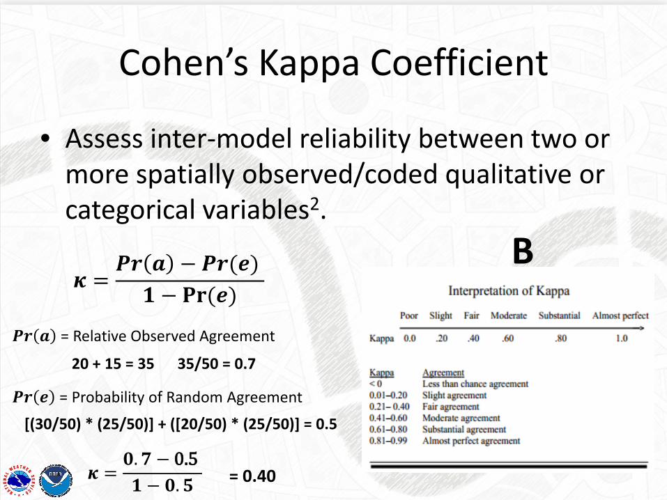
Cohen’s Kappa Coefficient
• Assess inter-model reliability between two or more spatially observed/coded qualitative or categorical variables2.
Yes No Totals
Yes 20 5 25
No 10 15 25
Totals 30 20 50
A
B𝜿𝜿 =
𝑷𝑷𝑷𝑷 𝒂𝒂 − 𝑷𝑷𝑷𝑷(𝒆𝒆)𝟖𝟖 − 𝐏𝐏𝐏𝐏(𝒆𝒆)
𝑷𝑷𝑷𝑷 𝒂𝒂 = Relative Observed Agreement
𝑷𝑷𝑷𝑷 𝒆𝒆 = Probability of Random Agreement
20 + 15 = 35 35/50 = 0.7
[(30/50) * (25/50)] + ([20/50) * (25/50)] = 0.5
𝜿𝜿 =𝟎𝟎.𝟕𝟕 − 0.5𝟖𝟖 − 𝟎𝟎.𝟓𝟓 = 0.40

Minor Moderate
Major Record
Ƙ = 0.97Ƙ = 0.82
Ƙ = 0.81 Ƙ = 0.82

Fig. 2
• Unedited FESM Flood Extents had substantial to near perfect agreement.– Record Stage performed the strongest on average across all sites (Austin, TX outlier)
– Moderate Flood Stage was weakest on average across all 6 sites (moderate agreement)
• Using water impact location descriptions & FEMA DFIRM maps, edited flood extents (Fig. 2) had near perfect to substantial agreement.– Excluding the minor and moderate stages for Frankfort, KY (High substantial agreement)
• Kappa could be raised further with local knowledge of Trumbo Bottom Area.– Significant improvement for Alexandria, LA site in Bayou Maria Basin– Moderate Flood Stage still lowest on average but above 0.8 (near perfect)
Results
Flood Walls
Flood Walls
Backwater Flooding
Backwater Flooding
Flood Wall &
Backwater Flooding
Flood Wall &
Backwater Flooding
HEC-RAS Modeling
Issues
HEC-RAS Modeling
Issues
Fig. 1

Flood Pixel Classification Accuracy
• FCA = Pixels of FloodCorrect
(Pixels of FloodCorrect + Pixels of FloodOmission + Pixels of FloodCommission )
∑ ∑ ∑∑
++=
)111213(13
PixelCountPixelCountPixelCountPixelCount
FCA
A series of flood classification accuracy graphs comparing unedited FESM Extentsand edited FESM Extents against the accepted AHPS Extents were generated for:
- Minor - Moderate - Major - Record

0.68
0.790.78
0.85 0.85
0.64
0.740.80

Conclusions• FESM/ArcGIS Methodology deemed spatially accurate
– Effort vs. Cost Analysis• 70-98% FCA accurate and acceptable statistically • Completed in a week or less (starting from scratch) • With data in place & practice, can be as fast as 1-3
hours for raw flood area output & no QC
• Mapping Accuracy & Kappa can be successfully increased through quality control measures:– Set to match current Impact Statements – E19s– FEMA DFIRM Data– River Forecast Center Agreement– Emergency Manager & Local Water Authority Agreement
• Future Work– Test more sites with current methodology
• Quantify QC improvements thru Classification and Kappa values– Develop internal AGOL website for critical partner access.

Cited Sources
http://arcg.is/1L00Wvm
1. Gall, M., Boruff, B., and Cutter, S. (2007). ”Assessing Flood Hazard Zones in the Absence of Digital Floodplain Maps: Comparison of Alternative Approaches.” Nat. Hazards Rev., 8(1), 1–12.
2. Jeffrey D. Colby, Karen A. Mulcahy, and Yong Wang, 2000. Modeling flooding extent from Hurricane Floyd in the coastal plains of North Carolina. Global Environmental Change Part B: Environmental Hazards. 2(4), 157-168. http://dx.doi.org/10.1016/S1464-2867(01)00012-2.
3. Michener, William & Houhoulis Paula. “Identification and Assessment of Natural Disturbances in Forested Ecosystems: The Role in GIS and Remote Sensing.” 1995 (http://www.ncgia.ucsb.edu/conf/SANTA_FE_CDROM/sf_papers/michener_william/michener.html)
4. Short, Nicholas. Accuracy Assessment. (http://www.fas.org/irp/imint/docs/rst/Sect13/Sect13_3.html)5. Qi, S., Brown, D. G., Tian, Q., Jiang, L., Zhao, T., & Bergen, K. M. (2009). Inundation Extent and Flood Frequency Mapping Using LANDSAT
Imagery and Digital Elevation Models. GIScience & Remote Sensing, 46(1), 101-127.6. Viera, Anthony, MD & Garrett, Joanne, PhD. “Understanding Interobserver Agreement: The Kappa Statistic.” Family Medicine. May 2005.
(http://www1.cs.columbia.edu/~julia/courses/CS6998/Interrater_agreement.Kappa_statistic.pdf)7. Wilson, M. D., & Atkinson, P. M. (2005). The use of elevation data in flood inundation modelling: a comparison of ERS interferometric SAR
and combined contour and differential GPS data. International Journal of River Basin Management, 3(1), 3-20.8. Weiger, Ben. NWS Flood Inundation Mapping Services, 2008. Bayou Vermillion River Conference.
(http://www.srh.noaa.gov/media/lch/outreach/052808/6BenWeiger.pdf)
ESRI Water Conference 2016 Austin, TX