six sigma and its implementation
DESCRIPTION
Basic Concept of Six Sigma and Its ImplementationTRANSCRIPT

SIX SIGMA AND ITS IMPLEMENTATION ON
THE PROJECT

Six Sigma
Six Sigma
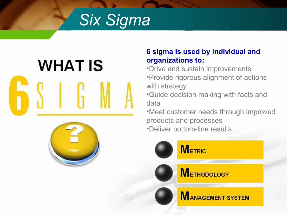
6 sigma is used by individual and organizations to:•Drive and sustain improvements•Provide rigorous alignment of actions with strategy•Guide decision making with facts and data•Meet customer needs through improved products and processes•Deliver bottom-line results

Six Sigma
Sigma Level Defect.10-6
± 1σ
± 2σ
± 3σ
± 4σ
± 5σ
± 6σ
697,700
308,700
66,810
6,210
233
3.4

Six Sigma

Six Sigma

Six Sigma Companies

The Six Sigma Evolutionary Timeline
1736: French mathematician Abraham de Moivre publishes an article introducing the normal curve.
1896: Italian sociologist Vilfredo Alfredo Pareto introduces the 80/20 rule and the Pareto distribution in Cours d’Economie Politique.
1924: Walter A. Shewhart introduces the control chart and the distinction of special vs. common cause variation as contributors to process problems.
1941: Alex Osborn, head of BBDO Advertising, fathers a widely-adopted set of rules for “brainstorming”.
1949: U. S. DOD issues Military Procedure MIL-P-1629, Procedures for Performing a Failure Mode Effects and Criticality Analysis.
1960: Kaoru Ishikawa introduces his now famous cause-and-effect diagram.
1818: Gauss uses the normal curve to explore the mathematics of error analysis for measurement, probability analysis, and hypothesis testing.
1970s: Imai develop Dr. Deming concept called 14 keys of Deming or called kaizen in Japanese.
1986: Bill Smith, a senior engineer and scientist introduces the concept of Six Sigma at Motorola
1994: Larry Bossidy launches Six Sigma at Allied Signal.
1995: Jack Welch launches Six Sigma at GE.

CustomerCompetitive Price
High Quality ProductsOn-time Delivery, etc
Company Profitability
Repeat BusinessGrowth/Expansion
Cash !!Cash !!$
Value !!Value !!
Some ProfitSome ProfitBigger ProfitBigger Profit
1
2
31
2
3
Price - Cost = ProfitPrice - Cost = Profit
Price to Sell
Price to Sell
Cost to ProduceCost to Produce
KEY BUSINESS CONCEPT OF SIX SIGMA

Six Sigma Methods Production
DesignService
Purchase
HRM
Administration
QualityDepart.
Management
M & S
IT
Where can Six Sigma be applied?

COPQ against sales revenue
COPQ (Cost of Poor Quality)
Sigma Level DPMO COPQ as sales percentile
1-sigma 691.462 (very low competitive) N/A
2-sigma 308.538 (Average Indonesia’s Industry) N/A
3-sigma 66.807 25-40% of sales
4-sigma 6.210 (Average USA’s Industry) 15-25% of sales
5-sigma 233 (Average Japan’s Industry) 5-15% of sales
6-sigma 3,4 (World Class Industry) < 1% of sales

$600$500$450$380$200
$2500
$1200
$700
$170
Cost Benefit
1996
Cost Benefit
1997
Cost Benefit
1998
Cost Benefit
1999
Cost Benefit
2000
6 Sigma Cost6 Sigma ProductivityDelighting Customers
SUCCESS STORY IN SIX SIGMASUCCESS STORY IN SIX SIGMA General ElectricGeneral Electric
$2500
$3.0B
$0.5B
$2.5B$2.5B

Dupont Chronology
Periode Description Sigma
Before six sigma Dupont Total Cost of Poor Quality= 20 -30 % of revenue
About 3 sigma
Implementing Cost of Implementing Six Sigma = $ 20 million
-
1999 Q1 Pilot Project Six Sigma on Specialty Chemicals started-Revenues $ 1.5 Billions-Target $ 80 million savings (5% dari revenues)
1999 Q2 40 Black Belts done for training and start for project
1999 Q4 Total saving $ 35 million (initial target $ 25 million) 2.3% of Revenue17.7% COPQ4 Sigma
2000 Q4 Total saving $ 100 million (initial target $ 80 million) 6.7% of Revenue13.3% COPQ5 sigma

Difficult-to-Reach FruitDesign for Six Sigma (DFSS)
Middle FruitSix Sigma tools
Lower Fruit7 Basic Tools of QC
Ground FruitLogic and Intuition
66σσ Basic Concept Basic Concept

3 sigma level company 6 sigma level company
• <25∼40% of sales is failure cost. • 5% of the sales is failure cost.
• Having 66,807 defects per million. • 3.4 defects per million.
• Depends on the detect to find
defect.
• Focusing on process not to produce
defects.
• Believes that high quality is expensive. • Realizes that high quality creates
low cost.
• Not available of systematic
approach.
• Uses know-how of measurement,
analysis, improvement & control.
• Benchmarking against competing
companies.
• Benchmarking to the best
in the world.• Believes 99% is good enough.
4 sigma Level? 1misspelled word per 30pages of newspaper.
5 sigma Level? 1misspelled word in a set of encyclopedias.
6 sigma Level? 1misseplled word in all of the books contained in a small library.
• Define CTQ’s internally.
• Believes 99% unacceptable.
66σσ Basic Concept Basic Concept

• It is important to understand the difference between accuracy and precision• Sigma is a measure of variationvariation (the data spread)
• It is a statistical measure unit displaying a process capability and the
measured sigma value is expressed by DPU(Defect Per Unit), PPM
• It is said that the process with higher sigma value is the process having smaller
defects
• The more increase the sigma value, the more decrease the quality cost and
Cycle Time
The concept of sigma
1σ
μ USL
3σT
Inflection Point
: The size or a standard deviation shows the distances between the inflection point and the mean. We could say the process has 3 sigma capability if 3 deviations are fit table between the target and the specification limit.
Understanding Basic Concept of Statistics

What does variation mean?
• Variation means that a process does not produce the same result (the “Y”)
every time.
• Some variation will exist in all processes.
• Variation directly affects customer experiences.
Customers do Customers do notnot feel averages! feel averages!
-10
-5
0
5
10
15
20

Measuring Process Performance
• Customers want their pizza delivered fast!
• Guarantee = “30 minutes or less”
• What if we measured performance and found an average delivery time of 23.5 minutes?– On-time performance is great, right?– Our customers must be happy with us, right?
The pizza delivery example. . .

How often are we delivering on time?Answer: Look at the variation!
• Managing by the average doesn’t tell the whole story. The average and the variation together show what’s happening.
s
x
30 min. or less
0 10 20 30 40 50
The pizza delivery example. . .

Reduce Variation to Improve Performance
• Sigma level measures how often we meet (or fail to meet) the requirement(s) of our customer(s).
s
x
30 min. or less
0 10 20 30 40 50
How many standard deviations can you “fit” within customer expectations?

SIX SIGMA Basic Concept
• All work occurs in a system of interconnected processes
• Variation exists in all processes
• Understanding and reducing variation are the keys to improving customer satisfaction and reducing costs

Y = f(χ)Question 1), Which one should we focus on the Y or X?
Question 2), Is needed to test and audit Y continually if the X is good?
• Y
• Dependent Variable
• Output
• Effect
• Symptom
• Monitor
• X1 … Xn
• Independent Variable
• Input
• Cause
• Problem
• Control object
6 Sigma activity is concerned about the problem happened(in the sector of
manufacturing and non manufacturing). They could be improved by focusing
the factor which causes the problem.

Steps Activity
Measurement
4. Understanding process capability for ‘Y’
5. Clarifying measurement method of ‘Y’
6. Specific description of Target object for improving
against ‘Y’
Focus
Y
Y
Y
Analysis 7. Clarifying Target for improving ‘Y’
8. Clarifying factors which affect ‘Y’
Y
X1 .... Xn
Improvement9. Extract the vital few factors through screening
10. Understanding correlation of vital few factors
11. Process optimization and confirmation experiment
X1 .... Xn
Vital Few X1
Vital Few X1
Control12. Confirm measurement system for ‘X’
13. Selection method how to control vital few factors
14. Build up process control system & audit for vital few
Vital Few X1
Vital Few X1
Vital Few X1
6 Sigma activity with 5 steps of D-M-A-I-C, will pass through the major 14 steps. 6 Sigma activity have D-M-A-I-C process breaking down the problem through the condition analysis, finding
the potential causal factor , and improving the vital few factors After the condition identification, we have the first action about the part being improved at first, and then we
proceed continually the improvement activity at the next step.
Define1. Clarifying improvement target object.
2. Forecasting improvement effect.
3. CTQ selection for products and process. Y
The Approach of 6 Sigma Step

6 Sigma Roles6 Sigma Roles

SIX SIGMA CHALLENGES
• Six sigma less suitable for innovation.• Six sigma emphasize process and cost,
while innovation constitutes something new in which cost consuming.
• Six sigma only analyzing quantitative data, qualitative data must be converted to quantitative.

Six Sigma DMAIC Process
Develop Charter and Business Case
Map Existing Process
Collect Voice of the Customer
Specify CTQs / Requirements
Measure CTQs / Requirements
Determine Process Stability
Determine Process Capability
Calculate Baseline Sigma
Refine Problem Statement
Identify Root Causes
Quantify Root Causes
Verify Root Causes
Institutionalize Improvement
Control Deployment
Quantify Financial Results
Present Final Project Results and Lessons Learned
Close Project
Select Solution (Including Trade Studies, Cost/Benefit Analysis)
Design Solution
Pilot Solution
Implement Solution
Define
Measure
Analyze
Improve
Control
DMAIC = Define, Measure, Analyze, Improve and Control

66σσ Methodology Methodology

DefineDefine
Defining the “Project Y”
Translate the external CTQ’s into internal product requirements or “Project Y”.
Example:
Project YCTQVoice of theCustomer
The range must heat to the setting chosen
The refrigerator must stay dry
Call-takers must be available to answer calls
Answer rate(% of incoming calls
answered within 20 seconds)
Call-takers must answer 95% of all incoming calls
within 20 seconds (telephone promptness)
Calibration angleof the thermostat
A thermostat setting of 350° must result in a
350° oven cavity
Foam densityNo sweat

Process MappingProcess Mapping
Start Finish
1 2
Process Targets and SpecificationsExperimental
Input ParametersTarget Upper Spec. Lower Spec.
Y = f (X)
(SOP ) = Standard Operating Parameters( N ) = Noise Parameters( X ) = Controllable Process Parameters
Add the operating specification and process targetsFor the controllable variable input

Courtesy of Daraius Patell
Continue to ask “Why?” until you Reach the Root Cause…...
Structure TreeExample
RPM
Losses
Inductance
OD
Core length
STATOR
ASSEMBLY
ROTOR
Electromagnetic
Mechanical
Area A
Area B
Lamination
Endrings

Cause & Effect DiagramCause & Effect Diagram•The final diagram will look like a fishbone with the backbone displaying every known
variable (Measurement, Method, Machine, People, Materials, Environment).
Measurement Method Machine
People Materials Environment

33
Why-why
Diagram

Measurement Measurement Determine Process Capability for Determine Process Capability for
Project YProject YDetermining process capability for your "Project Y" allows you to do several important things.
– Establish a baseline for comparing the improvement of your product or process.
– Quantify the ability of your process to produce output that meets the performance standard.
– Determine if there is a technology or control problem.
– Understand process capabilities for the design of future processes for DFSS (Design for Six Sigma) projects.
– Compare your process with others (internally and externally) to judge relative performance.
• Define the problem in mathematical terms
• Predict probability of producing defects

Measurement Measurement
Determine Current Sigma LevelDetermine Current Sigma Level

Used to break down problem into manageable groups to identify root cause
or area of focus.
Process for creating a Structure Tree:• List your problem statement on the left hand side of the page.
• Break the problem down into causes by asking ‘Why?’ and record on tree branches. Typical categories of causes include:
Technical TransactionalManpower PeopleMachine PriceMaterial ProductMethod PromotionMeasurement Physical Distribution
• Assign a High, Medium or Low impact to each branch and select the highest impact branch.
• Continue breaking down by asking ‘Why?’ until you reach the root cause.
Structure Tree

What is a “Measurement System”?
- Everything associated with taking measurements: the people, measurement tool, material, method
and environment is known as --
Think of the “Measurement System” as a sub-process that can add additional variation to measurement data. The goal is to use a measurement process that has the smallest
amount of measurement error as possible.
ObservationsMeasurementsData
Inputs Outputs Inputs Outputs
-- The “Measurement System”.
Parts
More Frequently Asked Questions More Frequently Asked Questions About Measurement DataAbout Measurement Data

ObservedProcessVariation
Actual Process Variation
Measurement Variation
Long TermProcess Variation
σ lt
Short TermProcess Variation
σst
Within Sample
Variation
Variation due to
Measurement Equipment
Variation due to
Operators
Accuracy Linearity ReproducibilityStabilityRepeatability
Sources of Measurement System VariationSources of Measurement System Variation
The Gage R&R methods we will study in this class will provide estimates of the total measurement variation, the variation attributed to measurement equipment repeatability and the variation attributed to the appraisers.

Acceptable if less than 20%
Conditional if between 20% to 30%
Unacceptable if greater than 30%
Evaluation Criteria for Evaluation Criteria for %GR&R and %Study Variation%GR&R and %Study Variation
Beware of the risk associated with using data acquired from an unacceptable
measurement process.
Beware of the risk associated with using data acquired from an unacceptable
measurement process.
σ2gage = σ2
repeatability + σ2reproducibility
Repeatability: The variation in measurements taken by a single person or instrument on the same or replicate item and under the same conditions.Reproducibility: the variation induced when different operators, instruments, or laboratories measure the same or replicate specimen.

AnalyzeAnalyze
Hypothesis Test (for variables)
Hypothesis Test (for attributes)

CorrectDecision
CorrectDecision
Type 1Error
α
Type 2Error
β
Ho Ha
Ho
Ha
True
Accept
The ratio which isbeing “Ha” even if it’s false.
Where “β” is usually set up at 10%.
The ratio which isbeing rejected Ho even
though certain thing is true where “ α” is α error.
(usually 5%)
*Ho(Null Hypothesis) is assumed to be true. This is like the defendant being assumed to be innocent.
Ha(Alternative Hypothesis is alternatives the Null Hypothesis. Ha is the one that must be proved.

Data Types
Variable Discrete
◎ t-Test (Compares means less than 2 population)
◎ ANOVA (Compares variances more than 2 population)
◎ F-Test (Compares variances of two population)
◎ Chi Square (Compares counts and frequencies.)
Before t-Test/ANOVA, confirm thehomogeneity of variance conductingF-Test
the gap delta(δ)
The larger Means and expected gap is getting,the more different two variances of average in population.
T

• The tool depends on the data type. We use ANOVA when we have categorical input(s) and a continuous response.
Continuous Categorical
Ca
teg
ori
ca
l C
on
tin
uo
us
Dependent Variable (Y)
Ind
epe
nd
en
t V
aria
ble
(X
)
Regression
ANOVA
LogisticRegression
Chi-Square (χ2)Test

Variance Homogeneity Testing Means Testing
1.One population variance testing
2.Two population variances testing
3.Testing of population variances for more than two (Normal distribution)
4. Testing of population variances for more than two (Non-Normal distribution)
Chi Square
F
Homogeneity ofVariance▶Bartlett’s Test
Homogeneity ofVariance▶Levene’s Test
1.One population Mean testing
1) When we know σ of the population 2) When we know σ of the population
2.Two population Mean testing
1) When they know σ1 and σ2
2) When they don’t know σ1 and σ2
① σ1 = σ2
② σ1 ≠ σ2
Normal distribution( 1 - Sample Z )
T distribution( 1 - Sample t )
Normal distribution
T distribution( 2 - Sample t )
The type of Hypothesis

What is DOE ?
• DOE is more than just a statistical DOE is more than just a statistical technique. technique.
• It is the combination of effective planning, It is the combination of effective planning, discipline, subject matter knowledge and discipline, subject matter knowledge and statistical methods that make the statistical methods that make the experiment a success.experiment a success.
ImprovementImprovement

DOE Steps
1.1. Define the objective of the experiment.Define the objective of the experiment.
2.2. Select the response and input factors.Select the response and input factors.
3.3. Determine the resources required.Determine the resources required.
4.4. Select suitable experiment design Select suitable experiment design matrix and analysis strategy. matrix and analysis strategy.
5.5. Perform the experiment and record Perform the experiment and record data.data.
6.6. Analyse the data, draw conclusions, Analyse the data, draw conclusions, and perform confirmation runs.and perform confirmation runs.
Good Good
planning is planning is
critical to critical to
success!success!

Basic Concepts in DOEBasic Concepts in DOEPressurePressure
SpeedSpeedProcessProcess
Quality Characteristic (Y)Quality Characteristic (Y)
++--
Pr
118Ave +
58Ave -12++901046--701034-+905210+-7051
YPr
x SpdSpdSpdPrRun
79 Y = 8
2 0 6
y = 8 + Pr + 3 x ( Pr Spd)y = 8 + Pr + 3 x ( Pr Spd)^̂
ProcessProcess
Process Process ModelModel
DO
ED
OE

FMEAFMEAFailure Modes and Effects Analysis is a systematic method for identifying, analyzing, prioritizing, and documenting potential failure modes and their effects on a system, product, or process.

SAMPLES
A B C D E
· Controllable factors
- Assignable causes
- Adjustable
- Special
· Uncontrollable factors
- Common causes
- Noise
- Inherent causes
• SPC has been traditionally used to monitor and control the output of processes.
In this application, we are measuring the dimensions of finished parts or
characteristics of finished assemblies.
• Six Sigma Quality focuses on moving control upstream to the leverage input characteristic for Y. If we can
measure and control the vital few X’s, control of Y should be assured.
INPUT
Controller α/2
α/2
X
Lower Control Limit
Upper Control Limit
ProcessCapability
Desired Output
OUTPUTPROCESS
The Logic of SPC(Statistical Process Control)?
L M N O P
10050Subgroup 0
0.5
0.0
-0.5
Sam
ple
Mea
n
Mean=0.001188
UCL=0.4384
LCL=-0.4360
1.0
0.5
0.0
Sa
mp
le R
ang
e
11 1
R=0.2325
UCL=0.7596
LCL=0
Xbar/R Chart for Sealing Angle Line #2
Control Control

Types of Control Charts Types of Control Charts
Variables Charts for monitoring continuous X’s
• Average & Range X bar & R n < 10 typically 3~5
• Averages & Std Deviation
X bar & σ
n ≥ 10
• Median & Range X & R n < 10 typically 3~5
• Individual & Moving Range XmR n = 1
Attributes Charts for monitoring discrete X’s
• Fraction Defective P Chart typically n ≥ 50 tracks DPU/DPU
• Number Defective np Chart n ≥ 50 (constant) tracks # def
• Number of Defects
c Chart
c > 5
• Number of Def/Unit
U Chart
n variable
• In order to select the appropriate control chart for monitoring your process, first
determine if your key process variables (X’s) are continuous or discrete. There are
control charts for both continuous data and discrete data.

Control Chart
12
10
8
•
••
•
•
••
•
••• ••
••
•
••
•
•
Week
Upper Control Limit = Ave + 3 x Std Dev14
13
7
6Lower Control Limit = Ave - 3 x Std Dev
Central Line = Average
Note: Control limits should be established using subgroup standard deviation

Six Sigma DMAICImplementation Project
Example

Date …………………
Department / TeamPrepared : …………..
Project title
G Manager Pres. Dir.Director
Mgr.
6σ
Ch
am
pio
n R
evie
wFin
al R
ep
ort
Contents
1. Define Step 2. Measure Step3. Analysis Step4. Improvement Step5. Control Step
-Attachment

Define Step

PJT Name
Perio
d
TeamNameDiv./Dept:
Breakthrough KPI Current World Best Target
Main Improvement Object
Team Formation (Related Department Involved)
Name Dept. Level Role
Quantitative
Qualitative
Expected
Results
How to do ?Why ?(* Selection Background)
New Idea for Target Achievement
Engineer
Ap
pro
val
Ka Part Ka Group Project Registration
Neck Point

CIAMD
4500
5000
Current Current Target Target Unit: (Nm3/day)
11%
How to do:
Target Saving cost:
OthersElec
tricO2N2LNG
0.00700.06050.12900.13090.1650 1.412.326.226.633.5
100.0 98.6 86.3 60.1 33.5
0.5
0.4
0.3
0.2
0.1
0.0
100
80
60
40
20
0
Defect
CountPercentCum %
Per
cent
Cou
nt
Energy Usage Price
Expected resultBackground
General Background

Start Finish
1 2
Process Targets and SpecificationsExperimental
Input ParametersTarget Upper Spec. Lower Spec.
Y = f (X)
(SOP ) = Standard Operating Parameters( N ) = Noise Parameters( X ) = Controllable Process Parameters
Add the operating specification and process targetsFor the controllable variable input
Process Mapping
CIAMD

SIPOC – Suppliers, Inputs, Process, Outputs, Customers
You obtain inputs from suppliers, add value through your process, and provide an output that meets or exceeds your customer's requirements.
Pro
ces
s U
nd
erst
and
ing
CIAMD

Measure Step

F(x) Machine
Man
Big Y X1 X2 X3
Brainstorming Potential X’s List
Material
Material
CIADM

Sampling
Training
Gage R&R
Result
Conduct a training……How to see what kind …….. Defect that happened in process.Purpose : find out the operator ability.
Conduct Gage R&R for 4 men to know the judgment capability (in different times & do not know the inspection result of each other) --> Repeat 2 times for each persons
% Gage R&R : 0 %
acceptable
Date:………
Collected 12 ea Sampling
Observed ProcessVariation
Measurement Process Variation
Sample M a nM a nMachineMethodMaterial
To determine if the measurement error is To determine if the measurement error is small and acceptable relative to the small and acceptable relative to the
process variation, we can process variation, we can use Gage R&R study.use Gage R&R study.
Gage R & R
CIADM

Units of Measureµµ
Center of the bar
Smooth curve interconnecting the center of each bar
Process CapabilityCurrent Condition
1 2 3 4 5 6
1.0
0.5
1.5
2.0
2.5
Z Sh
ift
Proc
ess
Con
trol
Good
Poor
Technology
GoodPoor
Block A
Block C
Block B
Block D
Four Block Diagram
Z Shift
A : Poor control, inadequate technology B : Must control the process better, technology is fineC : Process control is good, inadequate technologyD : World class
Current Target
CIADM

Factor Detail Analysis PlanSchedule
Mar 2nd Week Mar 3rd Week Mar 4th Week
X1.3
X1.1 Inspect correlation between “Y” and inspector for each group
Analysis khole / dimensionHeight, diameter, angle etc,
X1.2
X1.4
Analysis Plan
CIADM

Analyze Step
CID MA
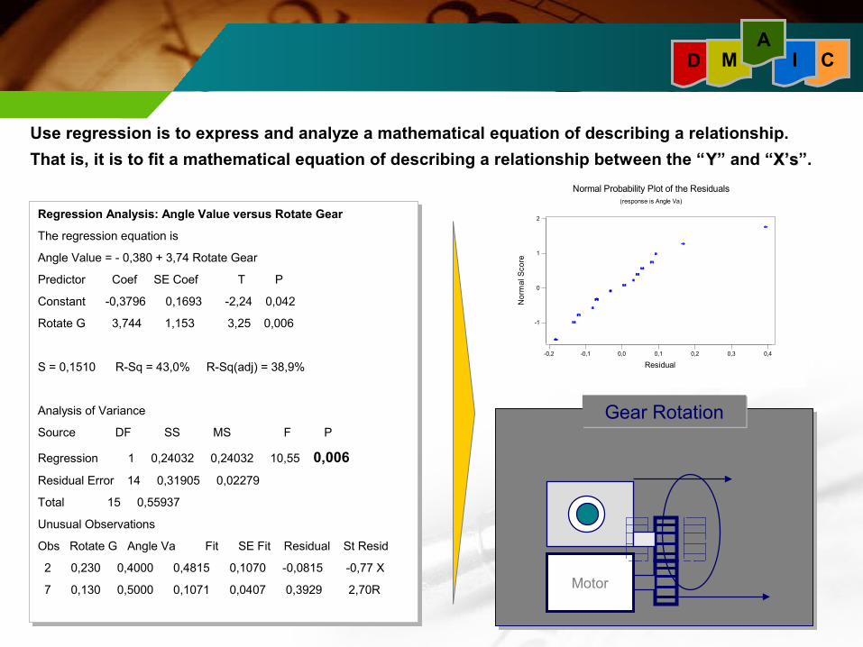
Regression Analysis: Angle Value versus Rotate Gear
The regression equation is
Angle Value = - 0,380 + 3,74 Rotate Gear
Predictor Coef SE Coef T P
Constant -0,3796 0,1693 -2,24 0,042
Rotate G 3,744 1,153 3,25 0,006
S = 0,1510 R-Sq = 43,0% R-Sq(adj) = 38,9%
Analysis of Variance
Source DF SS MS F P
Regression 1 0,24032 0,24032 10,55 0,006
Residual Error 14 0,31905 0,02279
Total 15 0,55937
Unusual Observations
Obs Rotate G Angle Va Fit SE Fit Residual St Resid
2 0,230 0,4000 0,4815 0,1070 -0,0815 -0,77 X
7 0,130 0,5000 0,1071 0,0407 0,3929 2,70R
-0,2 -0,1 0,0 0,1 0,2 0,3 0,4
-1
0
1
2
Nor
mal
Sco
re
Residual
Normal Probability Plot of the Residuals(response is Angle Va)
Motor
Gear RotationGear Rotation
Use regression is to express and analyze a mathematical equation of describing a relationship.
That is, it is to fit a mathematical equation of describing a relationship between the “YY” and “X’sX’s”.

One-way ANOVA: Gr.A - 3, Gr.A - 4, Gr.B - 3, Gr.B - 4, Gr.C - 3, Gr.C - 4Analysis of Variance
Source DF SS MS F P
Factor 5 0.8761 0.1752 2.59 0.030
Error 102 6.8897 0.0675
Total 107 7.7659
Individual 95% CIs For Mean
Based on Pooled StDev
Level N Mean StDev -------+---------+---------+---------
Gr.A - 3 18 0.0572 0.3029 (-------*-------)
Gr.A - 4 18 -0.1217 0.2427 (-------*-------)
Gr.B - 3 18 0.0839 0.2231 (--------*-------)
Gr.B - 4 18 -0.1183 0.2403 (-------*-------)
Gr.C - 3 18 0.0156 0.2796 (-------*-------)
Gr.C - 4 18 0.0967 0.2626 (-------*--------)
-------+---------+---------+---------
Pooled StDev = 0.2599 -0.15 0.00 0.15
P-Value: 0.242A-Squared: 0.452
Anderson-Darling Normality Test
N: 18StDev: 0.302865Average: 0.0572222
0.50.0-0.5
.999
.99
.95
.80
.50
.20
.05
.01
.001
Pro
bab
ility
Gr.A - 3
Normal Probability Plot
See from sealing angle specifications there’s no problem, cause all operator adjustmentStill in range (-0.5o ~ 0.5o). But there’s a significant effect both of them seeing by characteristic variation result, each operator have a different mean adjustment.
Since p-value < 0.05;Ho (reject), Ha (accept). That is we can claim there’sa difference between the levelOf adhesive
Gr.
C -
4
Gr.
C -
3
Gr.
B -
4
Gr.
B -
3
Gr.
A -
4
Gr.
A -
3
0.5
0.0
-0.5
Boxplots of Gr.A - 3 - Gr.C - 4(means are indicated by solid circles)
UCL
LCL
ScreenManual Adjustment
Operator Adjustment
Target Line
We represent characterized variation “Y”“Y” by the total sum of square, then this method is to find
what the factor’s level which influence enormously is, comparing both of them.
CID MA

CID MA
Factor Detail Analysis Content Result ConclusionAnalysis Purpose
Selected as Vital “X”
P = 0.000
Selected as Vital “X”
X1.1 Find most effected to “ Y “
X1.2
Find most effected to “ Y “
P = 0.000
Selected as Vital “X”
Bottle Neck
Regression, to compare Dew Point and Purge Flow rate
X1.3
X1.4 Regression, to compare Dew Point and Out Air Temperature
Find most effected to “ Y “
Find most effected to “ Y “
ANOVA, to compare Dew Point and Heating Time
ANOVA, to compare Dew Point and Drying Time
P = 0.000
P = 0.003
Analysis Result

Improve Step

CD M AI
Design of Experiment
Full Factorial Design
Factors: 3 Base Design: 3, 8Runs: 8 Replicates: 1Blocks: 1 Center pts (total): 0
Drying TIme
Flow rate
10 hour
6 hourHeating Time
12 hour
4 hour
520 m3/hr
Level 2Level 1Factors
810 m3/hr
The Improve phase identifies a solution and confirms that the proposedSolution will meet or exceed the improvement goals of the project.StdOrder RunOrder CenterPt Blocks Flow rate Heating Time Drying Time Result
8 1 1 1 810 6 12 -90.2
5 2 1 1 600 4 12 -52.6
1 3 1 1 600 4 10 -56.4
7 4 1 1 600 6 12 -57.6
2 5 1 1 810 4 10 -89.2
3 6 1 1 600 6 10 -68.1
6 7 1 1 810 4 12 -85.3
4 8 1 1 810 6 10 91.3

Heating Time : 4 hour
Drying Time : 10 hour
Flow rate : 520 m3/hour
Optimize Condition:
CD M AI

-40-50-60-70-80
LSL USLProcess Data
Sample N 24StDev (Within) 4.29772StDev (Ov erall) 8.60376
LSL -80.00000Target *USL -40.00000Sample Mean -64.18750
Potential (Within) Capability
CCpk 1.55
Ov erall Capability
Z.Bench 1.81Z.LSL 1.84Z.USL 2.81Ppk
Z.Bench
0.61Cpm *
3.68Z.LSL 3.68Z.USL 5.63Cpk 1.23
Observ ed Performance% < LSL 0.00% > USL 0.00% Total 0.00
Exp. Within Performance% < LSL 0.01% > USL 0.00% Total 0.01
Exp. Ov erall Performance% < LSL 3.30% > USL 0.25% Total 3.55
WithinOverall
Process Capabi l i ty of Dew Point
-40-50-60-70-80
LSL USLProcess Data
Sample N 24StDev (Within) 4.29772StDev (Ov erall) 8.60376
LSL -80.00000Target *USL -40.00000Sample Mean -60.00000
Potential (Within) Capability
CCpk 1.55
Ov erall Capability
Z.Bench 2.05Z.LSL 2.32Z.USL 2.32Ppk
Z.Bench
0.77Cpm *
4.51Z.LSL 4.65Z.USL 4.65Cpk 1.55
Observ ed Performance% < LSL 0.00% > USL 0.00% Total 0.00
Exp. Within Performance% < LSL 0.00% > USL 0.00% Total 0.00
Exp. Ov erall Performance% < LSL 1.00% > USL 1.00% Total 2.01
WithinOverall
Process Capabi l i t y of Dew Point
1 2 3 4 5 6
1.0
0.5
1.5
2.0
2.5
Z Sh
ift
Proc
ess
Con
trol
Good
Poor
Technology
GoodPoor
Block A
Block C
Block B
Block D
Four Block Diagram
Z Shift
Current Target
Improvement Result
CD M AI

4500
5000
Current Current Target Target
Result
8%
4600
Result Result
92%92%
Cost Saving: US$
Improvement Result
CD M AI

Control Step

I
ProcessInput
Controller
Controllable factors:- Miss adjust causes- Adjustable check- Pad control- Education
Group Member
Process CapabilityDesiredOutput
X
Upper Control Limit
Lower Control Limit●
●
Six Sigma Quality focuses on moving control upstream to the leverage input characteristic
for Y. If we can measure and control the vital few X’s, control of Y should be assured.
10050Subgroup 0
0.5
0.0
-0.5
Sam
ple
Mea
n
Mean=0.001188
UCL=0.4384
LCL=-0.4360
1.0
0.5
0.0
Sam
ple
Ran
ge
11 1
R=0.2325
UCL=0.7596
LCL=0
Xbar/R Chart for Sealing Angle Line #2
Output
Process Standard Change
CD M A

IC
D M A
P Chart enables us to control our process using statistical method's to signal when
process adjustments are needed.
50403020100
0.004
0.003
0.002
0.001
0.000
Sample Number
Pro
por
tion
P Chart for Stem Crack
P=0.001198
UCL=0.002466
LCL=0

15105Subgroup 0
10.2
10.1
10.0
9.9
9.8
9.7
Sam
ple
Mea
n
1
Mean=9.943
UCL=10.13
LCL=9.755
1.0
0.5
0.0
Sam
ple
Ran
ge
R=0.5594
UCL=1.016
LCL=0.1030
Xbar/R Chart for Cullet Speed
X-bar/R Chart use to control daily average for CTQ.
CTQ’s daily control data

Six Sigma ProjectExample

Date 20 MAY 2009Team : Galvanize
Prepared by : Imam Mudawam
Optimalkan pemakaian Zinc
Pada Proses Galvanize
Prod Mgr CEO.
Work Mgr
6σ
Cham
pio
n R
evie
wFi
nal
Rep
ort
Contents
1. Define Step 2. Measure Step3. Analysis Step4. Improvement Step5. Control Step
ISKDCNG

PJTName
Period
TeamName
Div./Dept: CONST./GALV.
Breakthrough
KPI Current World Best TargetMain Improvement Object
Team Formation (Related Department Involved)
Name Dept. Level Role
Quantitative
Qualitative
Expected Results
How to do ?Why ?(* Selection Background)
New Idea for Target Achievement
CEO
Appro
val
Work Mgr Prod Mgr
Neck Point
Optimalkan Pemakaian Zinc
Z Shift: - 1.86.
Imam M
Lukman
Banbang
Spv
Supv
Form
• Ketebalan Galvanize sesuai standard.
Amin Form Member
Leader
Leader
Member
Rp / kg
Rp / kg
Slamet Member
Fab
Galv
Galv
Galv
Qc
CIAMD
Project Registration
D
M
A
I
C
Schedule- Making Theme Reg.- Analyzing Aging Root-Caused
- Determine Potential X List- Find Current situation- Find Vital X by analyzing Potential X
-Find Improvement idea-Confirmation run
-Process Control by Monitoring Aging Amount
May – W5
Junl – W5
Jul –W5
Optimalkan Pemakaian ZincPada Proses Galvanize
Saving Zinc Rp. 295 Juta /Tahun
Galvanize
Reduce cost
Hans Ga Supv
Form
Member
Sept –W3
Sept –W5
Galvanize183.6 micr.
Galvanize130 micron
280240200160120
LSL Target USL
LSL 100Target 130USL 150Sample Mean 183.649Sample N 35StDev (Within) 18.0955StDev (Ov erall) 31.8811
Process Data
Z.LSL 2.62Z.USL -1.06Ppk -0.35Low er CL -0.49Upper CL -0.21Cpm 0.11Low er CL 0.09
Z.Bench -1.86Low er CL -2.59Z.LSL 4.62Z.USL -1.86Cpk -0.62Low er CL -0.80Upper CL -0.44
Z.Bench -1.07Low er CL -2.11
Ov erall Capability
Potential (Within) Capability
PPM < LSL 0.00PPM > USL 885714.29PPM Total 885714.29
Observ ed PerformancePPM < LSL 1.89PPM > USL 968521.55PPM Total 968523.44
Exp. Within PerformancePPM < LSL 4348.13PPM > USL 854388.04PPM Total 858736.18
Exp. Ov erall Performance
WithinOv erall
Pr ocess Capabi l i t y of t 6 .5mm +(using 95.0% confidence)
Worksheet: Worksheet 3; 11/13/2009
ISK DC NG

General BackgroundCIAM
D
• Hasil proses Galvanize ketebalannya melebihi standar yang ditentukan dalam ASTM- A123 / A123M.
• Tujuan Proyek ini untuk dapat mengoptimalkan ketebalan lapisan zinc pada hasil proses galvanize.
Produk tebal 6.0s/d….mm
sample mean micron 183.6 84.2 83.6Percent 52.3 24.0 23.8Cum % 52.3 76.2 100.0
Ketebalan material
Mat
erial
t.1.
5s/d
3.0m
m
Mater
ial t.
3.5s
/d6.
0mm
Mate
rial t
.6.5
s/d ..
.mm
400
300
200
100
0
100
80
60
40
20
0
sam
ple
mea
n m
icro
n
Perc
ent
Pareto Char t of Ketebalan mater ial
Worksheet: Worksheet 3; 10/14/2009

Big Y X1 X2 X3
Brainstorming Potential X’s List CIAM
D
Degrising
Pickling 1 & 2
Material
Konsentrasi BasaCaustic Soda
Base Metal
Konsentrasi Keasaman
Optimalkan pemakaian ZincPada Proses Galvanize
Temperatur
Waktu Pencelupan
Komposisi kimia
Ketebalan
1
Hcl

Optimalkan Pemakaian ZincPada proses Galvanize
Fluxing Konsentrasi Keasaman
Big Y X1 X2 X3
1
Temperatur
Brainstorming Potential X’s List CIAM
D
Zinc Amunium Chloride
DippingAluminium Alloy
Zinc Ingot
Temperatur
Komposisi Campuran
Waktu pencelupan

In doing gage R&R we take 2 times repeat in check
Gage R&R take from 2 Inspector who check this sample of Galvanize coating thickness in 10 chek point
Decide operator who take Gage R&R
Do Gage R&R
Change Method,measurement, etc
Analyze Result Gage R&R
Next Step
NG ; Total Gage R&R > 20%
OK ; Total Gage R&R < 20%
Measure Step - GAGE R&RCIA
MD

Gage R&R
Gage R&R < 20%Acceptable
CIAM
D
Sample pengukuran ketebalan galvanize sebanyak 2 sample dengan 30 titik pengukuran , tiap sampel diambil 15 titik pengukuran Diukur secara berurutan dan secara acak oleh dua orang operator .
The result of Gage R&R total is 14.67 % the acceptance percentage is bellow 20% (< 20 % ) , meanwhile the result of measurement between < 20 %, it accepted.
Study Var %Study Var
Source StdDev (SD) (6 * SD) (%SV)Total Gage R&R 2.0064 12.0384 14.67 Repeatability 2.0064 12.0384 14.67 Reproducibility 0.0000 0.0000 0.00 oprtr 0.0000 0.0000 0.00Part-To-Part 13.5243 81.1460 98.92Total Variation 13.6724 82.0341 100.00
Part-to-PartReprodRepeatGage R&R
100
50
0
Per
cent
% Cont ribut ion% Study Var
8
4
0Sam
ple
Ran
ge
_R=2.633
UCL= 8.604
LCL= 0
A B
110
100
90Sam
ple
Mea
n
__X=96.67UCL= 101.62
LCL= 91.71
A B
321
110
100
90
part no
BA
110
100
90
oprt r
321
110
100
90
part no
Ave
rage
AB
oprt r
Gage name: Date of study :
Reported by : Tolerance: Misc:
Com ponents of Variat ion
R Chart by oprt r
Xbar Chart by oprt r
m easure by part no
m easure by oprt r
oprt r * part no I nteract ion
OPERATOR PENGUKURAN KETEBALAN GALVANIZE
Worksheet: Worksheet 3; 9/9/2009

CIAM
DCurrent Condition
Rata rata ketebalan Galvanize pada produk dengan ketebalan > 6.0 mm saat ini mencapai 183.6 micron , berdasarkan data dari tgl.20 Juni 09 Sampai 27 Juni 09 ,jumlah sample 35 , alat ukur menggunakan COATING THICKNESS DIGITAL merek TIME - TYPE TT 220 .Untuk mendapatkan ketebalan sesuai target yang diinginkan grafik harus bergeser kekiri , dan harus mengurangi keteba- Pelapisan Galvanize yang sesuai standard ASTM A 123/A 123M antara ( 100 s/d 150 ) micron .
300250200150100
99
95
90
80
70605040
30
20
10
5
1
t 6.5mm +
Perc
ent
Mean 183.6StDev 31.88N 35AD 1.706P-Value <0.005
Probabi l i t y Plot Ketebalan Galvanize mater ial 6 .5mm s/ d .......dstNormal - 95% CI
Worksheet: Worksheet 3; 7/1/2009
KETEBALAN GALVANIZE
280240200160120
LSL Target USL
LSL 100Target 130USL 150Sample Mean 183.649Sample N 35StDev (Within) 18.0955StDev (Ov erall) 31.8811
Process Data
Z.LSL 2.62Z.USL -1.06Ppk -0.35Low er CL -0.49Upper CL -0.21Cpm 0.11Low er CL 0.09
Z.Bench -1.86Low er CL -2.59Z.LSL 4.62Z.USL -1.86Cpk -0.62Low er CL -0.80Upper CL -0.44
Z.Bench -1.07Low er CL -2.11
Ov erall Capability
Potential (Within) Capability
PPM < LSL 0.00PPM > USL 885714.29PPM Total 885714.29
Observ ed PerformancePPM < LSL 1.89PPM > USL 968521.55PPM Total 968523.44
Exp. Within PerformancePPM < LSL 4348.13PPM > USL 854388.04PPM Total 858736.18
Exp. Ov erall Performance
WithinOv erall
Process Capabi l i t y of t 6 .5mm +(using 95.0% confidence)
Worksheet: Worksheet 3; 11/13/2009

Four Block Diagram CIAM
D
Nilai sigma level saat ini adalah – 1.86 σ, target yang ingin dicapai 4.5 σ
A B
C
0.5
1.0
1.5
2.0
2.5
1 2 3 4 5 6
Z sh
iftP
roce
ss C
ontro
l
Good
Poor
Poor GoodZ st
Technology
Position of Current Condition was column C , it was mean :
PROCESS CONTROL IS GOOD,BUT TECHNOLOGY (METHOD) IS BAD
EXPLANATION
D
SIGMA TARGET
SIGMA TARGET
Sigma current – 1.86

CIA
MD
WAKTU PENCELUPAN
Optimalkan pemakaian ZincPada proses Galvanize
F(x) x
Analysis
TEMPERATUR ZINC
KETEBALAN GALVANIZE

Optimalkan pemakaian zinc pada proses Galvanize (Continuous)
Waktu Pencelupan
Y Factor (x) Type Tools
Analyze – Type of factor & Tools Using CIA
MD
CONTINUE REGRESION

Regression Analysis: Ketbln.Galva versus Wktu fluxing, Wktu.deeping, ...
* Wktu.deeping is (essentially) constant* Wktu.deeping has been removed from the equation.* NOTE * All values in column are identical.* Temp.deeping is (essentially) constant* Temp.deeping has been removed from the equation.
The regression equation isKetbln.Galvanize (micron ) = 110 - 1.17 Wktu fluxing
Predictor Coef SE Coef T P VIFConstant 109.667 3.658 29.98 0.000Wktu fluxing -1.1668 0.4555 -2.56 0.034 1.000
S = 4.13685 R-Sq = 45.1% R-Sq(adj) = 38.2%
Analysis of Variance
Source DF SS MS F PRegression 1 112.32 112.32 6.56 0.034Residual Error 8 136.91 17.11Total 9 249.22
Unusual Observations
Wktu Ketbln.GalvanizeObs fluxing (micron ) Fit SE Fit Residual St Resid 1 3.0 114.00 106.17 2.43 7.83 2.34R
R denotes an observation with a large standardized residual.
Durbin-Watson statistic = 1.69422
Analysis Waktu Fluxing ( Regresion )
CIA
MD
Ketebalan Galvanize VS Waktu Fluxing
Nilai p-value < 0.05, maka Ho ditolak, yang menandakan variabel waktu Fluxing berpengaruh terhadap ketebalan galvanize.
Nilai p-value < 0.05, maka Ho ditolak, yang menandakan variabel waktu Fluxing berpengaruh terhadap ketebalan galvanize.

Regression Analysis: Ktbl . Galva versus Tmprt deepin, Wkt.deeping, ...
* Wkt.deeping is (essentially) constant* Wkt.deeping has been removed from the equation.
* NOTE * All values in column are identical.
* Wkt.fluxing is (essentially) constant* Wkt.fluxing has been removed from the equation.
The regression equation isKtbl . Galvanize (micron ) = - 98 + 0.443 Tmprt deeping
Predictor Coef SE Coef T P VIFConstant -98.4 157.1 -0.63 0.548Tmprt deeping 0.4428 0.3562 1.24 0.249 1.000
S = 6.47038 R-Sq = 16.2% R-Sq(adj) = 5.7%
Analysis of Variance
Source DF SS MS F PRegression 1 64.70 64.70 1.55 0.249Residual Error 8 334.93 41.87Total 9 399.63
Durbin-Watson statistic = 1.36705
Analysis Temperatur Dipping ( Regresion )
CIA
MD
Ketebalan Galvanize VS Temperatur Zinc
Nilai p-value > 0.05, maka Ho diterima, yang menandakan variabel temperatur tidak berpengaruh terhadap ketebalan galvanize.
Nilai p-value > 0.05, maka Ho diterima, yang menandakan variabel temperatur tidak berpengaruh terhadap ketebalan galvanize.

Regression Analysis: Ktbalan Galvanize micron versus Waktu deeping
The regression equation isKtbalan Galvanize micron = 43.7 + 19.9 Waktu deeping
Predictor Coef SE Coef T P VIFConstant 43.674 5.279 8.27 0.000Waktu deeping 19.9082 0.6573 30.29 0.000 1.000
S = 5.96979 R-Sq = 99.1% R-Sq(adj) = 99.0%
Analysis of Variance
Source DF SS MS F PRegression 1 32698 32698 917.49 0.000Residual Error 8 285 36Total 9 32983
Durbin-Watson statistic = 2.41646
Analysis Waktu Dipping ( Regresion )
CIA
MD
Waktu Dipping VS Ketebalan Galvanize
Nilai p-value < 0.05, maka Ho ditolak, yang menandakan variabel waktu dipping berpengaruh terhadap ketebalan galvanize.
Nilai p-value < 0.05, maka Ho ditolak, yang menandakan variabel waktu dipping berpengaruh terhadap ketebalan galvanize.

CIA
MD
Selected not Vital View
Item Content Result Remarks
Selected as Vital View
Galvanizing
P = 0.034
P = 0.024
P = 0.000
Waktu Fluxing
Temperatur Dipping
Waktu Dipping
Analysis Result ( Regression )
Selected not Vital View
Berdasarkan data diatas variabel waktu Dipping paling berpengaruh terhadap hasil ketebalan pada proses galvanize (99%)

CImprovementIAMD
• Berdasarkan hasil analisa, untuk produk dengan ketebalan 6 mm didapatkan hubungan linier antara lamanya waktu pencelupan dengan hasil ketebalan galvanize.
• Grafik di bawah ini dapat dijadikan acuan untuk menentukan tebal galvanize yang diinginkan.
HUBUNGAN WAKTU PENCELUPAN DAN KETEBALAN GALVANIZEPADA PRODUK DENGAN KETEBALAN 6 mm
0
1020
3040
5060
70
8090
100110
120130
140
150160
170180
190
200210
220230
240250
260
0 1 2 3 4 5 6 7 8 9 10 11
Waktu Pencelupan (menit)
Ke
teb
ala
n G
alv
an
is (
mic
ron
)
Standar 6mm
Y = 43.7 + 19.9 x

94
CImprovementIAMD
Catatan : Proses improvement masih sedang berjalan dan akan dilaporkan kemudian hari.


Session Start : 23.01.02
□○ Theme Register
□○ Team Organization
□○ Process Map
□○ Cpk Analysis(Current)
□○ Problem Description
□○ CTQ Selection
□○ Measurable Y Value
Selection
□○ 4 Block Diagram
□○ Brainstorming
□○ Logic Tree Analysis
□○ Analysis by Minitab
□○ Process Benchmarking
□○ CTQ Selection
□○ Process Map
□○ ANOVA
□○ Regression Analysis
□○ Factor Level Decision
□○ DOE
□○ Statistical Interpretation
□○ Data Gathering & Analysis
□○ Main Factor Analysis
□○ Hypothesis Test
□○ ANOVA
□○ Control Chart
□○ Rational Tolerance
selection
□○ Document Control plan
□○ Training Process Controller
□○ CTQ Process Monitoring
System set up
Session Finished :
□○ Y Identification
□○ Gauge R&R
□○ 4 Block Focus(Zst & Zshift)
□○ Problem analysis
reaffirmation
□○ Statistical skill of Y
□○ Graphical skill of Y
□○ Gap Analysis
□○ The 1st improvement of
X(Factor)
□○ Conclusion(the fixed X
factor)
□○ Test plan
□○ Control Plan
Implementation
□○ CTQ Process Monitoring
System Build-Up
□○ Double check of all the
problems
Measurement Analysis Improvement Control
Session Start : Session Start : Session Start :
Main Schedule
Session Finished : Session Finished : Session Finished :
Measure Measure Define Define Improve Improve Control Control Analyse Analyse

A period of time taken off by an employee which is neither planned or authorised
Definition Of Defect
DEFINITION
Sickness
Unauthorised absence
Lateness
DEFECT TYPES
Payment for overtime to cover absence = £800,000:00 paLoss in revenue due to lost production = £700,000:00 pa (est)Adverse morale issuesDeterioration in productivity and quality
VALUE
Measure Measure Define Define Improve Improve Control Control Analyse Analyse

Absence Logic Tree
Absence
Management Style
Time With Company
Sex
=CTQ’s
Age
Guidelines
Team Leader
Section
Accidents
Morale issues
Cleanliness
Repetitive Work
Employee
Target Setting
Environment
Method
Consistent Approach
Use Of Policy
Shift Pattern
Measure Measure Define Define Improve Improve Control Control Analyse Analyse

Graph shows reduction in absence, since the beginning of the project (DEC) spotlight effect has reduced absence. One problem we do have is the calculation of absence data there is a difference between the HR data collection method and the tube plant data collection method.
Sigma Level Calculation
Using The Percentage Defective (4.605%) We Calculated The DPMO Since Merger
DPMO = 46050
Using statistical tables the SIGMA LEVEL = 3.21
Measure Measure Define Define Improve Improve Control Control Analyse Analyse
-2
0
2
4
6
8
Tube 4.27 4.66 5.23 4.7 5.01 5.34 3.86 3.13 2.75
HR 4.31 5.22 5.86 4.56 5.09 5.02 3.97 3.45 2.72
Variance -0.04 -0.56 -0.63 0.14 -0.08 0.32 -0.11 -0.32 0.03
Jul Aug Sep Oct Nov Dec Jan Feb Mar Apr May Jun

VOC - Harp Questionnaire
219 People Questioned Across The Tube Plant
Answered by all employees.Name Marital StatusClock Number AgeDepartment ChildrenShift HomeTime with Company Job positionTime in current job
Have you taken any unauthorised time off since 5th July 2001? YES / NODo you currently have any warnings that relate to sickness or absence? YES / NODo you understand LGPDW's absence and sickness policy? YES / NODo you understand the affect of absence on our business? (e.g. cost, pressure on colleagues)
Only to be answered by employees with no absence historyHow do you think high absence levels affects your ability to do your job?What do you think of LG. PHILIPS Displays as an employer? Are you happy working for LGPDW?
Ask employee all questions below, and mark the score they give ie strongly agree = 10, agree = 5 and strongly disagree = 0.Do you think absence is due to Management style?Do you think absence is due to accidents in work?Do you think absence is due to the current shift pattern?Do you think absence is due to your working environment?If I was late for work, I would take the rest of the shift off because it still counts as an absenceAre there any other reasons that you think contribute to absence that are not listed above?
Measure Measure Define Define Improve Improve Control Control Analyse Analyse

Overall catchment area
Main catchment area
Catchment Area Of People Questioned
Measure Measure Define Define Improve Improve Control Control Analyse Analyse

Others
Job rotation
P ay rise
Music
Mgt attitude
A tt Bonus
12 5 14 33 51137
4.8 2.0 5.613.120.254.4
100.0 95.2 93.3 87.7 74.6 54.4
250
200
150
100
50
0
100
80
60
40
20
0
Defect
CountPercentCum %
Per
cent
Cou
nt
How would y ou tackle high absence?
Operators
Pareto’s Of Absence Data
Teambuilding
E xtra manning
gather info on
persis tan
t absentees
1 - 1Communication
A ttendance bonus
11224
10.010.020.020.040.0
100.0 90.0 80.0 60.0 40.0
10
5
0
100
80
60
40
20
0
Defect
CountPercentCum %
Per
cent
Cou
nt
How would y ou tackle absence?
Section Leaders
Conclusions
Operators would like to be paid
more to come to work
Operators see a problem in the
way they are treated by Mgt
Music might help??
Conclusions
Section Leaders see the benefit
in some form of attendance
bonus, but more emphasis on
communication and data
collection
Measure Measure Define Define Improve Improve Control Control Analyse Analyse

Pareto’s Of Absence Data
Others
deaths
car problems
accidents insid
e work
low morale
injury o
utside work
flexible fl
oatdays
sickness
fludomestic
1111223444
4.3 4.3 4.3 4.3 8.7 8.713.017.417.417.4
100.0 95.7 91.3 87.0 82.6 73.9 65.2 52.2 34.8 17.4
20
10
0
100
80
60
40
20
0
Defect
CountPercentCum %
Per
cent
Cou
nt
Main Reasons For Absence On Your Shif t
Others
experience
absence
poor maintenance
supply
low manning
1 1 2 3 511
4.3 4.3 8.713.021.747.8
100.0 95.7 91.3 82.6 69.6 47.8
20
10
0
100
80
60
40
20
0
Defect
CountPercentCum %
Per
cent
Cou
nt
Main issues af f ecting shif ts ability to meet output targets
Conclusions
No significant patterns have
emerged
Conclusions
Absence is not a major issue
Measure Measure Define Define Improve Improve Control Control Analyse Analyse

Analysis Using M System
ImproveImproveDefineDefine MeasureMeasure AnalyseAnalyse ControlControl
Time With Company
Sex
Age
Employee
NEXT STEP IS TO CARRY OUT ANALYSIS BYEMPLOYEE TO ESTABLISH IF THERE AREANY STATISTICAL DIFFERENCES
DATABASE WAS CREATED LOOKING AT THE NINE MONTH PERIOD (5th July-4th April) PRIOR TO AND DURING PROJECT
empno
Emp Namedept cd
Dept Name Grade shift noDistance Details
date_hired
Year/Month gender AgeAge
GroupCount
AbsenceAbs Occ
12345 A N OTHER1 81000 Tube Manufacturing Senior Engineer DT CF1 1AB 17/03/00 02/01 Male 34 D 0 012346 A N OTHER2 81000 Tube Manufacturing Senior Engineer DT CF1 1AB 06/10/99 02/06 Male 34 D 0 012347 A N OTHER3 81000 Tube Manufacturing Team Leader DT CF1 1AB 11/08/97 04/08 Male 33 D 3 112348 A N OTHER4 81100 Screen Production Section Leader T4 CF1 1AB 18/05/98 03/11 Male 51 H 0 012349 A N OTHER5 81100 Screen Production Section Leader T2 CF1 1AB 26/04/99 02/12 Male 42 F 1 112350 A N OTHER6 81100 Screen Production Section Leader T1 CF1 1AB 10/05/99 02/11 Male 41 F 0 012351 A N OTHER7 81100 Screen Production Section Leader DT CF1 1AB 20/04/98 03/12 Male 41 F 0 012352 A N OTHER8 81100 Screen Production Section Leader T2 CF1 1AB 06/10/97 04/06 Male 39 E 1 112353 A N OTHER9 81100 Screen Production Team Leader DT CF1 1AB 12/01/98 04/03 Male 39 E 0 012354 A N OTHER10 81100 Screen Production Technician DT CF1 1AB 06/10/97 04/06 Female 35 D 0 0
Time with Company Personal DetailsEmployment Details Unauthorised Absence

Analysis By Age
ImproveImproveDefineDefine MeasureMeasure AnalyseAnalyse ControlControl
Created Age Groupings
Age Group Age RangeA 16-20B 21-25C 26-30D 31-35E 36-40F 41+
Analysed Percent Absent By Age Group
Conclusions
There is a significance showing that
D = 31-35 and F = 41+ are more likely to
not to take unauthorised absence and that
B = 21-25 are more likely to take
unauthorised absence
Chi-Square Test: A, B, C, D, E, F
Expected counts are printed below observed counts
A B C D E F Total 1 188 175 183 132 91 62 831 183.80 187.26 182.08 125.12 94.06 58.68
2 25 42 28 13 18 6 132 29.20 29.74 28.92 19.88 14.94 9.32
Total 213 217 211 145 109 68 963
Chi-Sq = 0.096 + 0.802 + 0.005 + 0.378 + 0.099 + 0.188 + 0.603 + 5.050 + 0.029 + 2.378 + 0.626 + 1.183 = 11.438DF = 5,
P-Value = 0.043
19.35%
13.27%
8.97%
16.51%
8.82%
13.71%
11.74%
A B C D E F GrandTotal

Analysis By Gender
ImproveImproveDefineDefine MeasureMeasure AnalyseAnalyse ControlControl
Split By Gender Analysed Percent Absent By Gender
Conclusions
There is significance showing that a
male person would more likely take
unauthorised absence
Female Male Grand Total22.28% 30.88% 29.08%
157 526 68345 235 280
Chi-Square Test: F, M
Expected counts are printed below observed counts
F M Total 1 188 643 831 174.31 656.69
2 14 118 132 27.69 104.31
Total 202 761 963
Chi-Sq = 1.075 + 0.285 + 6.767 + 1.796 = 9.924DF = 1,
P-Value = 0.002
15.51%
13.71%
6.93%
Female Male Grand Total

Group RangeA <1YearB 1-2 YearsC 2-3 YearsD 3-4 YearsE >4 Years
Analysis By Time Served
ImproveImproveDefineDefine MeasureMeasure AnalyseAnalyse ControlControl
Analysed Percent Absent By Time Served
Conclusions
There is a significance in that
E = 4 years +
is more likely to take unauthorized
absence
Created Time Served Groupings
Chi-Square Test: A, B, C, D, E
Expected counts are printed below observed counts
A B C D E Total 1 117 129 151 324 110 831 113.04 126.85 154.46 314.97 121.67
2 14 18 28 41 31 132 17.96 20.15 24.54 50.03 19.33
Total 131 147 179 365 141 963
Chi-Sq = 0.138 + 0.036 + 0.078 + 0.259 + 1.120 + 0.872 + 0.229 + 0.489 + 1.630 + 7.050 = 11.902DF = 4,
P-Value = 0.018
12.24%
15.64%
11.23%
21.99%
13.71%
10.69%
A B C D E GrandTotal

Analysis By Department
ImproveImproveDefineDefine MeasureMeasure AnalyseAnalyse ControlControl
Conclusions
This shows that there is a significance in departments
A = Tube Material Warehouse, B = Design/Process Engineering,
C = Sputter section.
In which all are more likely to take unauthorised absence
Percent Absent By Sub GroupCreated Department Sub-GroupsGroup dept_cd Dept Name Total Abs NeverA 83210 Tube Material Warehouse 46.15% 6 7B 81400 Design/Process Engineering 35.71% 5 9C 81320 Sputter section 32.50% 13 27D 81310 Spin section 21.21% 7 26E 84120 Tube OQC section 16.13% 5 26
81140 Maintenance 1 section81510 Maintenance Section(2/3)81230 Gunseal and Exhaust section81330 I.T.C. section81340 Outgoing section81450 CS-Reinspection section81210 Assembly Section81220 Inner Dag section
I 84110 Tube IQC section 7.69% 1 12J 81240 1st Inspection section 5.63% 4 67
81110 Screen Coating section81120 Chemical section
L 81130 Shadow Mask Section 2.50% 2 78Average 12.72% 109 748
F
G
H
14.55%
13.68%
10.29%
47
284
61
8
45
7
K 5.45% 6 104
35.71%32.50%
21.21%
16.13%14.55%13.68%10.29%
7.69%5.63% 5.45%
2.50%
46.15%
A B C D E F G H I J K L

Analysis By Shift
ImproveImproveDefineDefine MeasureMeasure AnalyseAnalyse ControlControl

Improvement Suggestions
Improvement Actions/Suggestions by CTQ.
CTQ Proved By Improvement Recommendation
AgeProved By Chi Square Test
Use best fit when recruiting.
GenderProved By Chi Square Test
Use best fit when recruiting.
Length Of ServiceProved By Chi Square Test
Use best fit when recruiting.
Shift PatternProved By Chi Square Test
Build In More flexibility for day shift workers.
DepartmentProved By Chi Square Test
Compare Management Styles
MoraleProved By HARP Survey
New Incentive Scheme (Ongoing)
AccidentsProved By HARP Survey
New Health & Safety Structure In Place
EnvirionmentProved By HARP Survey
Music & Improved Rest Room Facilities
Management StyleProved By HARP Survey
Training Courses For Manager On Interpersonal Skills. Management Attitude Improvement Plan Next Slide
Aggressive Target SettingProved By HARP Survey
Unable to improve due to the nature of our business.
Measure Measure Define Define Improve Improve Control Control Analyse Analyse

Improvement Suggestions - Management Attitude
Measure Measure Define Define Improve Improve Control Control Analyse Analyse
AbsenceMorale
More Information
Team Building
Improved Interpersonal Skills
Treat Operators As Equal
More 1 To 1 Communication
Follow Correct Procedures
Improved Grading System
HIGH MORALE = LOW ABSENCE

Improvement Suggestions - Attendance Bonus
Measure Measure Define Define Improve Improve Control Control Analyse Analyse
£100 Per Year
Decided By Incentive Scheme Working Party
Deductions?
All Authorised Non- Sickness Absence
Paid Quarterly
Cash/Vouchers/Savings
All Absence Resulting In Warnings
Total Savings £1,086,000
Verbal -25%
Written - 50%
F Written - 100%
All Deductions For 1 Year From Date Of Warning

Output
MeasureMeasureDefineDefine ImproveImprove ControlControlAnalyseAnalyse
Initial Current
σ level 3.21 3.43
PPM (Month) 46021 27300
Loss (£) £117000 £69405
£47595Est. Monthly Saving of:(Based on hours lost)

Contents:
1. Define Step 2. Measure Step3. Analysis Step4. Improvement5. Control
Process Sterilization Capability Up
6σ
Ch
am
pio
n R
evie
wFin
al R
ep
ort

Background CIAMD
Develop working efficiency and found 6 Sigma6 Sigma control for free Salmonella in sterilization process.
0 100 200 300 400 500
-0.5
0.0
0.5
1.0Individual and MR Chart
Obser.
Ind
ivid
ual V
alu
e
Mean=-0.01707
UCL=0.7674
LCL=-0.8016
0.0
0.3
0.6
0.9
Mo
v.R
ang
e
R=0.2950
UCL=0.9638
LCL=0
480 490 500
Last 25 Observations
-0.6
-0.3
0.0
0.3
Observation Number
Va
lue
s
-0.5 0.5
Capability PlotProcess Tolerance
I I I
I I I
I ISpecifications
Within
Overall
-0.5 0.0 0.5
Normal Prob Plot
-0.5 0.0 0.5
Capability Histogram
WithinStDev:Cp:Cpk:
0.2615070.640.62
OverallStDev:Pp:Ppk:
0.2886170.580.56
Process Capability Sixpack for Sealing Angle Line #2
Process Capability Current Condition
2
0.65
1.5
0.51
Target Current
Cp
Cpk

D CIAM
Executing analysis with Logic Tree for sterile product.
Potential X’ List
Big Y X1 X2 X3
Sterile Product Machine Sterile Time Fixed
Rotate
Temp Warm
Hot > 97
Steam Supply Spec (6.5 ~ 9) bar
Pineapples Bracket Stand
Methods Automatic
Material
Juice pH
Manual

Gage R&R D CIAM
0.010.05
novi mMar 3rd,2006Sealing angle Line 2
Misc:Tolerance:
Reported by:Date of study:Gage name:
0
0.5
0.0
-0.5
CBA
Xbar Chart by Operator
Sam
ple
Mea
n
Mean=0.03017UCL=0.03706LCL=0.02327
0
0.010
0.005
0.000
CBA
R Chart by OperatorS
ampl
e R
ange
R=0.003667
UCL=0.01198
LCL=0
10 9 8 7 6 5 4 3 2 1
0.40.30.20.10.0
-0.1-0.2-0.3-0.4
Part
OperatorOperator*Part Interaction
Ave
rage
A B
C
CBA
0.40.30.20.10.0
-0.1-0.2-0.3-0.4
Operator
By Operator
10 9 8 7 6 5 4 3 2 1
0.40.30.20.10.0
-0.1-0.2-0.3-0.4
Part
By Part
%Contribution
%Study Var
Part-to-PartReprodRepeatGage R&R
100
50
0
Components of Variation
Per
cent
Gage R&R (ANOVA) for Measurement
Gage R&R %Contribution
Source VarComp (of VarComp)
Total Gage R&R 0.000020 0.03
Repeatability 0.000020 0.03
Reproducibility 0.000000 0.00
Operator 0.000000 0.00
Part-To-Part 0.077747 99.97
Total Variation 0.077767 100.00
StdDev Study Var %Study Var
Source (SD) (5.15*SD) (%SV)
Total Gage R&R 0.004437 0.02285 1.59
Repeatability 0.004425 0.02279 1.59
Reproducibility 0.000323 0.00166 0.12
Operator 0.000323 0.00166 0.12
Part-To-Part 0.278832 1.43598 99.99
Total Variation 0.278867 1.43616 100.00
Two-Way ANOVA Table With InteractionSource DF SS MS F P
Part 9 4.19852 0.466502 21530.8 0.000000.00000Operator 2 0.00004 0.000022 1.0 0.38742
Operator*Part 18 0.00039 0.000022 1.2 0.33365
Repeatability 30 0.00055 0.000018
Total 59 4.19950
If significant, P-value < 0.05 indicatesthat a part is having a variation forSome measuring
Ok for “product acceptance”considering a productstolerance.

D CIAM
Measurement
Through analysis of process capability , getting sigma level 1.85 1.85 σσ
1 2 3 4 5 6
1.0
0.5
1.5
2.0
2.5
Z Sh
ift
Proc
ess
Con
trol
Good
Poor
Technology
GoodPoor
Block A
Block C
Block B
Block D
Four Block Diagram
1.85 σ 4.5 σ
Z Shift
1.00.50.0-0.5-1.0
Target USLLSL
Angle Line #2Process Capability Analysis for Sealing
PPM Total
PPM > USL
PPM < LSL
PPM Total
PPM > USL
PPM < LSL
PPM Total
PPM > USL
PPM < LSL
Ppk
Z.LSL
Z.USL
Z.Bench
Cpm
CpkZ.LSLZ.USL
Z.Bench
StDev (Overall)
StDev (Within)
Sample N
Mean
LSL
Target
USL
83742.06
36602.01
47140.05
56399.74
24004.66
32395.08
4008.02
0.00
4008.02
0.56
1.67
1.79
1.38
0.58
0.621.851.98
1.59
0.288617
0.261507
499
-0.017074
-0.500000
0.000000
0.500000
Exp. "Overall" PerformanceExp. "Within" PerformanceObserved PerformanceOverall Capability
Potential (Within) Capability
Process Data
Within
Overall
Process capability for Sterile Product
A : Poor control, inadequate technology B : Must control the process better, technology is fineC : Process control is good, inadequate technologyD : World class
Target

Analysis - Regression D CIMA
Regression Analysis: Sterile product versus time and tempThe regression equation is
Sterile =0.000303 + 0.00113 time + 0.000060 temp
Predictor Coef SE Coef T P
Constant 0.0003033 0.0002999 1.01 0.345
Time 0.00112859 0.00003939 28.65 0.000Time 0.00112859 0.00003939 28.65 0.000
Temp 0.00006005 0.00005694 1.05 0.327
S = 0.0003891 R-Sq = 100.0% R-Sq(adj) = 100.0%
Analysis of Variance
Source DF SS MS F P
Regression 2 0.82500 0.41250 2.725E+06 0.000
Residual Error 7 0.00000 0.00000
Total 9 0.82500
Regression Analysis: Sterile product versus time and tempThe regression equation is
Sterile =0.000303 + 0.00113 time + 0.000060 temp
Predictor Coef SE Coef T P
Constant 0.0003033 0.0002999 1.01 0.345
Time 0.00112859 0.00003939 28.65 0.000Time 0.00112859 0.00003939 28.65 0.000
Temp 0.00006005 0.00005694 1.05 0.327
S = 0.0003891 R-Sq = 100.0% R-Sq(adj) = 100.0%
Analysis of Variance
Source DF SS MS F P
Regression 2 0.82500 0.41250 2.725E+06 0.000
Residual Error 7 0.00000 0.00000
Total 9 0.82500 0.00050.0000-0.0005
1
0
-1
No
rma
l Sco
re
Residual
Normal Probability Plot of the Residuals(response is Angle)
Use regression is to express and analyze a mathematical equation of describing a relationship. That is, it is
to fit a mathematical equation of describing a relationship between the “YY” and “X’sX’s”.
p-value < 0.05 : Significant factor
R2 and R2-adj are over 90% : which indicates a potentially good fit

Regression Analysis: Sterile product versus Steam supplyThe regression equation is
Sterile product = - 0,380 + 3,74 Steam supply
Predictor Coef SE Coef T P
Constant -0,3796 0,1693 -2,24 0,042
Steam Supply 3,744 1,153 3,25 0,006Steam Supply 3,744 1,153 3,25 0,006
S = 0,1510 R-Sq = 43,0% R-Sq(adj) = 38,9%
Analysis of Variance
Source DF SS MS F P
Regression 1 0,24032 0,24032 10,55 0,006
Residual Error 14 0,31905 0,02279
Total 15 0,55937
Regression Analysis: Sterile product versus Steam supplyThe regression equation is
Sterile product = - 0,380 + 3,74 Steam supply
Predictor Coef SE Coef T P
Constant -0,3796 0,1693 -2,24 0,042
Steam Supply 3,744 1,153 3,25 0,006Steam Supply 3,744 1,153 3,25 0,006
S = 0,1510 R-Sq = 43,0% R-Sq(adj) = 38,9%
Analysis of Variance
Source DF SS MS F P
Regression 1 0,24032 0,24032 10,55 0,006
Residual Error 14 0,31905 0,02279
Total 15 0,55937The P-value < 0.05Reject Ho ; Accept haThe P-value < 0.05Reject Ho ; Accept ha
Comparing of Sterile product and steam supply to find what the factor’ level’s which influence
enormously by represent characterized variation “Y”“Y” by the total sum of square.
Analysis – Regression D CIMA
0.30.20.10.0-0.1-0.2-0.3
4
3
2
1
0
Residual
Fre
quen
cy
Histogram of the Residuals(response is Cullet S)

Analysis – Chi-square D CIMA
Since P-Value >> 0.05; there’s no significantEffect between product sterile and factor.Since P-Value >> 0.05; there’s no significantEffect between product sterile and factor.
Conclusion:
◆ At least no one region is different, because a dependence exists. (P > 0.05)
◆ It no appears that the dependence may exist with Region 1 due to the large difference between the observed and the expected values.(must subtract the expected and observed values)
Conclusion:
◆ At least no one region is different, because a dependence exists. (P > 0.05)
◆ It no appears that the dependence may exist with Region 1 due to the large difference between the observed and the expected values.(must subtract the expected and observed values)
This Chi-Square is used to Test hypotheses about the frequency of occurrence of some event
happening with equal probability.
Chi-Square Test: matang, Stngh matang, juice Expected counts are printed below observed countsChi-Square contributions are printed below expected counts
Stngh matang matang juice Total OK 1000 995 1013 3008 1000.01 993.03 1014.96 0.000 0.004 0.004
NG 3 1 5 9
2.99 2.97 3.04 0.000 1.308 1.269
Total 1003 996 1018 3017
Chi-Sq = 2.585, DF = 2, P-Value = 0.2753 cells with expected counts less than 5.

Analysis – two sample T-test
D CIMA
Two-Sample T-Test and CI: Automatic, Chart
Two-sample T for Automatic vs Chart
N Mean StDev SE MeanAutomatic 12 14.70 1.47 0.42Manual 12 14.13 2.19 0.63
Difference = mu (Automatic) - mu (Chart)Estimate for difference: 0.56250095% CI for difference: (-1.030754, 2.155754)T-Test of difference = 0 (vs not =): T-Value = 0.74 P-Value = 0.469 DF = 19
Hypothesis tests help to determine if a difference is real, or if it could be due to chance
Dat
a
ChartAutomatic
19
18
17
16
15
14
13
12
11
Boxplot of Automat ic, Char t
There is no statistically significant differenceif the confidence interval for m1 - m2 does
include 0.0.

9
6.5
97
90107.5
Steam
Temp
Time
3
114
10
7
1215
0
Cube Plot (data means) for Salmonel la
D CM AImprovement – Response Surface Experiment
I
From the Main Effects Plot for the average of residue we conclude:
• Temp has the greatest effect on average residue
• Time has a lesser effect on average residue
• Steam supply shows little or no effect (within the test range)
on the average residue
Main Effects Plots for Main Effects Plots for Time, Temp & Steam supplyTime, Temp & Steam supply Average and Standard Deviation of Residue. Average and Standard Deviation of Residue.
• Salmonella : 0• Temp max : 97 oC• Time : 7.5 min• Steam : 6.5 bar
Best Condition:Best Condition:
Mea
n of
Sal
mon
ella
10.07.5
10.0
7.5
5.09790
9.06.5
10.0
7.5
5.0
Time Temp
St eam
Main Ef fects Plot ( data means) for Salmonel la

Improvement – Response Surface Experiment
D CM A I
Contour Plot
Interpretation: to make sterile product (no salmonella) move towards the center corner of the
Contour Plot (samonella = 00). Read off potential “Time” and “Temp” values that will provide Salmonella
< 2.
Lines of targetresponse for
“0” Salmonella
1. Get to know the condition giving lower salmonella.
2. To get the regular response, we realize what variables is important to control (temp & time)
3. Determine the level of independent variance needed for getting salmonella 00 (When temp is approximately 97oC)
Time
Tem
p
10.09.59.08.58.07.5
97
96
95
94
93
92
91
90
Hold ValuesSteam 6.5
Salmonella
4.5 - 7.07.0 - 9.59.5 - 12.0
12.0 - 14.5> 14.5
< 2.02.0 - 4.5
Contour Plot of Salmonel la vs Temp, Time

D CM A I
Generally, main effect is more important than interaction. If interaction is regarded as a important thing,
then interaction can be used as a factor of interaction and another interaction might be confounded.
96
Salm one l la
940
5
10
T em p
15
928 90910T im e
Hold ValuesSteam 6.5
Sur face Plot of Salmonel la vs Temp, Time
Improvement – Response Surface Experiment

Improvement – Result
D CM A I
1 2 3 4 5 6
1.0
0.5
1.5
2.0
2.5
Z Sh
ift
Proc
ess
Con
trol
Good
Poor
Technology
GoodPoor
Block A
Block C
Block B
Block D
Four Block Diagram
4.25 σ
Z Shift
1.85 σ
Improvement Result:
Saving Cost estimated: 2.7K U$/Year
0.500.250.00-0.25-0.50
Target USLLSL
Angle Line #2Process Capability Analysis for Sealing
PPM Total
PPM > USL
PPM < LSL
PPM Total
PPM > USL
PPM < LSL
PPM Total
PPM > USL
PPM < LSL
Ppk
Z.LSL
Z.USL
Z.Bench
Cpm
CpkZ.LSLZ.USL
Z.Bench
StDev (Overall)
StDev (Within)
Sample N
Mean
LSL
Target
USL
63.70
46.70
17.00
41.55
30.86
10.69
0.00
0.00
0.00
1.30
4.14
3.91
3.83
1.34
1.344.254.01
3.94
0.124193
0.121123
84
0.014762
-0.500000
0.000000
0.500000
Exp. "Overall" PerformanceExp. "Within" PerformanceObserved PerformanceOverall Capability
Potential (Within) Capability
Process Data
Within
Overall

Control D M A I
C
Process
InputController
Controllable factors:- Miss adjust causes- Adjustable check- Pad control- Education
Group Member
Process CapabilityDesiredOutput
X
Upper Control Limit
Lower Control Limit●
●
Six Sigma Quality focuses on moving control upstream to the leverage input characteristic for Y.
If we can measure and control the vital few X’s, control of Y should be assured.
10050Subgroup 0
0.5
0.0
-0.5
Sam
ple
Mea
n
Mean=0.001188
UCL=0.4384
LCL=-0.4360
1.0
0.5
0.0
Sam
ple
Ran
ge
11 1
R=0.2325
UCL=0.7596
LCL=0
Xbar/R Chart for Sealing Angle Line #2Output
Process Standard Change

Contents
6σ
Ch
am
pio
n R
evie
wD
MA
IC-S
tep
Rep
ort
1. DEFINE
2. MEASURE
3. ANALYSIS
4. IMPROVEMENT
5. CONTROL
Optimizing Material DIO

‘06 6σ Project Registration
PJT Name
Period TeamName
BreakthroughMain Improvement Object(KPI) Current World Best Target
New Idea for Target Achievement
Team Formation, Related Department Involved
Name Dept. Position Main Role
NECK POINT
How to do ?Why ?(* Selection Background)
Expected Results
Quantitative
Qualitative
Optimizing Material D I O
1. JIT delivery system for press part2. Door to door delivery for glass3. Hub delivery system from Korea4. Raw material issue control to process5. Weekly stock taking6. Minimize NG and rework stock in process
at end of the month7. PO issued based on the latest production
plan
1. D I O is one of key performance indicators in inventory management.
2. Good level of inventory will support production line in effective and efficient way.
3. Fluctuated material D I O
Current Condition
USL : 2.9LSL : -Means : 2.58091Sample N : 14Z Bench : 1.03
- Warehouse Inventory Amount D I O ( Days Inventory
Outstanding )2.6 days 2.3 days
- Working In Process Inventory Amount
1,117
K $
US
Current
1,050
Target - Continuous material supplies to production line
- All material used efficiently in production line
- Reduced warehouse and WIP inventory amount 1NG and rework stock in the end of month
2. Fluctuate production schedule
Just In Time PurchasingVendor Managed Inventory
K 67
3.53.02.52.01.5
USLUSL
Process Capability Analysis for C2
PPM Total
PPM > USL
PPM < LSL
PPM Total
PPM > USL
PPM < LSL
PPM Total
PPM > USL
PPM < LSL
Ppk
Z.LSL
Z.USL
Z.Bench
Cpm
Cpk
Z.LSL
Z.USL
Z.Bench
StDev (Overall)
StDev (Within)
Sample N
Mean
LSL
Target
USL
200815.40
200815.40
*
151989.40
151989.40
*
214285.71
214285.71
*
0.28
*
0.84
0.84
*
0.34
*
1.03
1.03
0.380447
0.310413
14
2.58091
*
*
2.90000
Exp. "Overall" PerformanceExp. "Within" PerformanceObserved PerformanceOverall Capability
Potential (Within) Capability
Process Data
Within
Overall

Background
DM A I C
One of the material inventory management control is DIO (Days Inventory Outstanding) that has the formula:
Inventory AmountMaterial DIO = ------------------------- X total days of current month Sales Amount
The elements of material DIO are: 1. Warehouse Inventory (Raw Material)2. Working In Process inventory (Semi Finished Goods )3. Material In Transit Inventory
This large amount and high DIO have some effects :
Risk in obsolescence, expired, lost, and defect
High inventory carrying cost
Current Material Inventory Condition :
Average Amount : $ K 1,117
D I O : 2.6 days
Optimizing inventory amount and D I O will bring material inventory management in a more efficient cost

DM A I C
X4X3X2X1Y X5
M. RATIO
Net BOMMaterial Price
Src. Performance
BOM Quantity
M. YIELD
CPT Price
Experience
Negotiation
Education
M. DIO
Material Loss
Net Req. Material
Material Cost Amt
Chemical
Others
Market Situation
Mat. Inv. Amt
Production Qty
Key Part
Sales Amt
Beginning Stock
Purchasing Qty
Ending Stock
Receive Amt
Total Days
In Transit Inv.
Warehouse Inv.
W I P Inv.
Sales Qty.
Current Month
Supply Condition
Glass
Mask
Press Part
Sub Mount
Process Part
Assy Part
Sales Target
Calculation Skill
Forecast Skill
Logic Tree

D M A I CLogic Tree
X4X3X2X1Y X5
Mat Inv Amt
In Transit Inv Delivery Sched.
Material DIO
Sales Amt
Sales Qty
Price
Warehouse Inv Experience
A
Education
Total Days
Stock
Bulb
B
Part Stock
Assy Stock
Current Month
Sales Target
Production Capa
Graphite G 72 B
D Y
CMA
Glass
M/Assy
Simulation Skill
Marketing Nego
Market Situation
W I P Inventory
YS
TCL Prod.
Comp. Supply
Sub Month
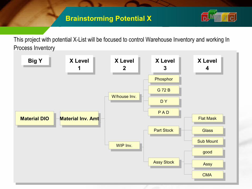
D M A I C
This project with potential X-List will be focused to control Warehouse Inventory and working In Process Inventory
X Level 2
X Level 2
D YD Y
Big YBig Y
Material DIOMaterial DIO
Assy StockAssy Stock
Part StockPart Stock
P A DP A D
GlassGlass
Sub MountSub Mount
Flat MaskFlat Mask
PhosphorPhosphor
G 72 BG 72 B
X Level 1
X Level 1
Material Inv. AmtMaterial Inv. Amt
W/house Inv.W/house Inv.
WIP Inv.WIP Inv.
X Level 3
X Level 3
X Level 4
X Level 4
AssyAssy
CMA CMA
goodgood
Brainstorming Potential X

DM
A I C
Gage R&R
StdDev Study Var %Study Var
Source (SD) (5.15*SD) (%SV)
Total Gage R&R 0.109148 0.56211 16.58 Repeatability 0.109046 0.56159 16.56
Reproducibility 0.004723 0.02432 0.72
Operator 0.004723 0.02432 0.72
Part-To-Part 0.649363 3.34422 98.62
Total Variation 0.658472 3.39113 100.00
Number of Distinct Categories = 8
Misc:Tolerance:Reported by:Date of study:Gage name:
0
4
3
2
321
Xbar Chart by Operator
Sam
ple
Mea
n
Mean=2.679UCL=2.724LCL=2.634
0
1.0
0.5
0.0
321
R Chart by Operator
Sam
ple
Ran
ge
R=0.02405UCL=0.07857LCL=0
1413121110 9 8 7 6 5 4 3 2 1
4
3
2
Part
OperatorOperator*Part Interaction
Ave
rage
1 2
3
321
4
3
2
Operator
By Operator
1413121110 9 8 7 6 5 4 3 2 1
4
3
2
Part
By Part
%Contribution
%Study Var %Tolerance
Part-to-PartReprodRepeatGage R&R
350
300
250
200
150
100
50
0
Components of Variation
Per
cent
Gage R&R (ANOVA) for Measure
To test validation of measurement , 3 (three) persons, twice inspection and 14 months calculation for material D I O has carried out, and the result was acceptable.
The result of Gage R&R total is 16.58, the acceptance percentage is below 20 (<20), meanwhile the result of measurement between <20, it accepted.
Gage R&R <20%
Acceptable
Gage R&R <20%
Acceptable
Gage R & R

Current Condition D MA I C
3.53.02.52.01.5
USLUSL
Process Capability Analysis for C2
PPM Total
PPM > USL
PPM < LSL
PPM Total
PPM > USL
PPM < LSL
PPM Total
PPM > USL
PPM < LSL
Ppk
Z.LSL
Z.USL
Z.Bench
Cpm
Cpk
Z.LSL
Z.USL
Z.Bench
StDev (Overall)
StDev (Within)
Sample N
Mean
LSL
Target
USL
200815.40
200815.40
*
151989.40
151989.40
*
214285.71
214285.71
*
0.28
*
0.84
0.84
*
0.34
*
1.03
1.03
0.380447
0.310413
14
2.58091
*
*
2.90000
Exp. "Overall" PerformanceExp. "Within" PerformanceObserved PerformanceOverall Capability
Potential (Within) Capability
Process Data
Within
Overall
Z-Bench : 1.03

Block Diagram D MA I C
Z shift has been identified , the Z shift will be 0.19, regarding this issue the target of the project is 4.5 sigma
A B
C
0.5
1.0
1.5
2.0
2.5
1 2 3 4 5 6
Z sh
iftP
roce
ss C
ontro
l
Good
Poor
Poor GoodZ st
Technology
Position of DIO was column C ,it was mean :
PROCESS CONTROL IS GOOD,BUT TECHNOLOGY (METHOD)
IS BAD
EXPLANATION
Z st : 1.03Z shift : Z st – Z lt : 1.03 – 0.84 : 0.19
Z st : 1.03Z shift : Z st – Z lt : 1.03 – 0.84 : 0.19
D

D M AI C
The Pareto analysis has been done, the result shows that tube stock, Furnace, CMA, and Assy have the highest contribution to WIP Assy Amount
WIP Assy Stock Analysis
Others
CPT Dongbang
Mount Assy
CMABulb
Bare Tube
14962 7725 33504 37174 48983165826 4.9 2.510.912.115.953.8
100.0 95.1 92.6 81.8 69.7 53.8
300000
200000
100000
0
100
80
60
40
20
0
Defect
CountPercentCum %
Per
cen
t
Cou
nt
Avg WIP Stock 1Q '04
Analysis
Bare TubeBare TubeBare TubeBare Tube
BulbBulbBulbBulb
CMACMACMACMA
45 % conveyor stock ($ 78 K)
F’ce StockC/V Stock
Mount AssyMount AssyMount AssyMount Assy
Safety Stock to secure supply
55 % ( $ 97 K) consists Of :- NG & rework, - Pending Lot- Remained Prod. Stock
Stock to keep production
2 shift Mount Assy Process
Pareto Chart for WIP Assy Inv.

D M AI CWIP Part Stock Analysis
OthersPhospor
Sub Mount
GlassMask
7375 10535 32501 50418179511 2.6 3.811.618.064.0
100.0 97.4 93.6 82.0 64.0
200000
100000
0
100
80
60
40
20
0
Defect
CountPercentCum %
Per
cen
t
Cou
nt
Pareto Chart for Desc.
The Pareto analysis result for WIP part stock shows that Mask Stock, Glass, Sub Mount and Phosphor have the highest contribution to WIP part Amount Analysis
Flat MaskFlat MaskFlat MaskFlat Mask
GlassGlassGlassGlass
Sub MountSub MountSub MountSub Mount
86 % stock at PT YSI($ 156 K)
Stockloading
PhosphorPhosphorPhosphorPhosphor
Safety Stock for aging time
14 % stock at SM ( $ 23 K)
- Annealing- Forming & Blackening
Mount Assy Process stock
High price
- Flat Mask (RM)
Pareto Chart for WIP Part Inv.

D M AI CWarehouse Stock Analysis
The Pareto analysis result for warehouse stock shows that Stock, Graphite, Phosphor and PAD have the highest contribution to Warehouse Stock amount Analysis
D YD YD YD Y
GraphiteGraphiteGraphiteGraphite
PhosphorPhosphorPhosphorPhosphor
Inner Supply
Hardly PO revision PO issued three month before
P A DP A DP A DP A D
- Quality Problem- Comp. Request to achieve sales target
Decreasing consumptions
- Revised Production Plan
GlassPAD
Phospor
GraphiteDY
1600717572396544144347520 9.910.824.425.629.3
100.0 90.1 79.3 54.8 29.3
150000
100000
50000
0
100
80
60
40
20
0
Defect
CountPercentCum %
Per
cen
t
Cou
nt
Pareto Chart for C1
Blue Stock
So frequently
Pareto Chart for W/House Inv.
Minimum order 2304 kg

D M AI C
Not Selected as Vital View
Selected as Vital View
Item High Amount Stock Remarks
Selected as Vital View
Selected as Vital View
Selected as Vital View W I P
Part
NG and rework Stock
Mask Stock outsourcing process
Warehouse
Assy
Analysis Result
Glass Stock
Sub Mount
Remained production stock & Pending lot
conveyor stock
Selected as Vital View
Not Selected as Vital View
Y D Y
G 72 B & G 355
P A D
Selected as Vital View
Selected as Vital View
Phosphor
Selected as Vital View

D M AI C
Bottle Neck1. High stock of NG, rework, pending lot in the end of month due to quality problem, sourcing team can not fully controlled this situation. Actually, it’s depend on process and quality performance.
Analysis Result
2. Outsourcing Mask Annealing process at Shin require more raw material stock to keep production and secure supply.
3. Frequently change production plan for CIT and Y DY quality problem cause influence high stock Y DY.

D M AI
C Improvement
Item Improvement Remarks
Mask Stock
- Identify and checking 3 days before closing
- Partial raw material delivery
Glass Stock
Stock
- Daily vendor managed inventory
- Communicate Stock to related dept and push for action
- Working closely with PCT Team to input remained stock
In the end of month
- Pending Lot
- Remained Prod. from March ‘04
Annealing Outsourced
- Optimized in out stock control
- Daily input glass to production line
- Communicate and push process to minimize stock
- Check stock condition & make any necessary action
Y D Y- Confirm I production plan - Best effort to match PCT Production Plan & actual
- Just In Time purchasing
PhosphorGraphite
- Improve Import delivery simulation skill
Weekly control
from March ‘04
Weekly control
from March ‘04
- Tightly control on ETD & ETA - Maintain actual delivery performance on SRS
from March ‘04
from March ‘04

D M AI
CImprovement Result
Result analysis after improvement actions : Z bench 2.60
2.92.72.52.32.11.91.71.5
USLUSL
Process Capability Analysis for DIO
PPM Total
PPM > USL
PPM < LSL
PPM Total
PPM > USL
PPM < LSL
PPM Total
PPM > USL
PPM < LSL
Ppk
Z.LSL
Z.USL
Z.Bench
Cpm
Cpk
Z.LSL
Z.USL
Z.Bench
StDev (Overall)
StDev (Within)
Sample N
Mean
LSL
Target
USL
1307.83
1307.83
*
4651.78
4651.78
*
0.00
0.00
*
1.00
*
3.01
3.01
*
0.87
*
2.60
2.60
0.215663
0.249574
6
2.25093
*
*
2.90000
Exp. "Overall" PerformanceExp. "Within" PerformanceObserved PerformanceOverall Capability
Potential (Within) Capability
Process Data
Within
Overall
Z-Bench : 2.60

D M AI
C Sigma Value
After improvement action, we can compare it with previous condition.Improved Condition is better than Previous Condition.
PREVIOUS CONDITION
A B
C0.5
1.0
1.5
2.0
2.5
1 2 3 4 5 6
Z s
hif
t
Pro
cess
Co
ntr
ol
Good
Poor
Poor GoodZ st
Technology
IMPROVED CONDITION
Sigma = 1.03
D
Z st : 2.60Z shift : Z st – Z lt : 2.60 – 3.01 : -0.41
Z st : 2.60Z shift : Z st – Z lt : 2.60 – 3.01 : -0.41
A B
C
0.5
1.0
1.5
2.0
2.5
1 2 3 4 5 6
Z sh
iftP
roce
ss C
ontro
l
Good
Poor
Poor GoodZ stTechnology
D
Z st : 1.03Z shift : Z st – Z lt : 1.03 – 0.84 : 0.19
Z st : 1.03Z shift : Z st – Z lt : 1.03 – 0.84 : 0.19
Sigma = 2.60

D M AI
C Saving Cost
1,117
K $
US
Current
1,050
Target
K 67 (6%)
TARGET
1,117
K $
US
Before
1,075
After
K 42 (4%)
RESULT
Previous Average Material Inventory Amount : $ K 1,117Current Average Material Inventory Amount : $ K 1,075 Saving Cost : $ K 42

D M A IC
Control
Below check sheets are applied to ensure and maintain the material inventory DIO stays optimized and some improvement activities stay controlled :
1. Mask daily inventory stock control at Shin
This is one of the application of vendor managed inventory (VMI)
2. Salvage glass daily input to process
3. Weekly Stock taking for warehouse and WIP (include Assy and Stock)
Desc. 31 1 2 3 4 5 6
F/MASK 5000 120000 120000 110000 100000 87000 80000
ANNEA 35447 33612 21740 19973 23373 25155 20373
FORM 2550 1961 3170 5149 2090 2095 8300
BLACK 7189 4841 7146 6972 6860 7207 2961
TOTAL 50186 160414 152056 142094 132323 121457 111634
F/MASK 5000 75000 75000 75000 75000 75000 75000
ANNEA 2933 2933 2933 2933 2933 2933 2933
FORM 0 0 0 0 0 0 0
BLACK 2790 2790 2790 2790 2790 2790 2790
TOTAL 10723 80723 80723 80723 80723 80723 80723
14"
20"
1. 2.
3.
1 2 3 4 5 6 7 8 9 10 11 12 13 14 15 16 17 18 19 20 21 22 23 24 25 26 27 28 29 30 31 Tt l
14 0 0 0 672 504 168 336 0 224 224 308 154 322 168 0 0 0 392 504 168 168 0 0 308 0 782 168 168 0 336 168 6242
20 0 0 0 72 266 248 310 0 0 180 72 272 0 0 0 0 72 0 0 72 208 0 0 192 416 200 64 62 0 548 64 3318
21 0 0 512 256 192 0 64 0 192 320 320 192 128 320 0 0 576 320 512 192 0 0 0 384 320 64 128 0 0 0 128 5120
0 0 512 # # 962 416 710 0 416 724 700 618 450 488 0 0 648 712 # # 432 376 0 0 884 736 # # 360 230 0 884 360 14680
1 2 3 4 5 6 7 8 9 10 11 12 13 14 15 16 17 18 19 20 21 22 23 24 25 26 27 28 29 30 31 Tt l
14 200 0 0 400 400 400 0 0 400 200 200 0 400 0 0 0 200 400 200 200 400 0 0 0 200 200 200 0 0 200 400 5200
20 0 0 81 0 261 90 270 0 90 0 0 180 0 0 0 0 0 0 0 0 0 0 270 0 180 270 270 180 0 180 90 2412
21 0 0 405 243 162 81 0 0 81 405 374 162 162 243 0 0 324 324 324 243 81 0 0 405 162 0 0 243 0 81 162 4667
200 0 486 643 823 571 270 0 571 605 574 342 562 243 0 0 524 724 524 443 481 0 270 405 542 470 470 423 0 461 652 12279
FUNNEL
PA NEL
JUMLAH
JUMLAH
Tanggal
Tanggal
1 153-113V DY 14" LG STD 0 0 488 2,432 -2,432 1.68205 0.00 820.842 153-276F DY HARTONO/SANKEN/VESTEL 0 0 0 0 0.00000 0.00 0.003 3024GAFA01C MASK FLAT 21" MULTI 20,000 20,000 2,191 80,000 -60,000 1.72214 34,442.80 145.704 3040GA0001A BASE 20" 202,103 202,103 0 202,103 0 0.02246 4,539.23 0.005 3040GA0006A BASE 14" 210,000 210,000 0 210,000 0 0.03620 7,602.00 0.006 3210GBAA01A FRAME SUPPORT 14" 0 0 4,284 0 0 0.12900 0.00 552.647 3210GBEA01A FRAME SUPPORT 20" 0 0 1,920 0 0 0.58850 0.00 1,129.928 3210GBFA01A FRAME SUPPORT 21" 0 0 3,120 0 0 0.63900 0.00 1,993.689 3300GB0001A PLATE COMPENSATION 0 0 0 0 0 0.63900 0.00 0.00
10 3300GB0001B PLATE COMPENSATION 10,000 10,000 0 10,000 0 0.00428 42.80 0.0011 3300GB0002A PLATE COMPENSATION 20,000 20,000 0 20,000 0 0.00299 59.80 0.0012 3300GC0001A B-S PLATE 20" 0 0 20,000 10,000 -10,000 0.01220 0.00 244.0013 3740GA0001A LEAD PROTECT 20" 12,500 12,500 11,500 12,500 0 0.01182 147.75 135.93
No Part No Description Act.Gd Inv. Book PMS Gap U/PRICEProcess REMARKSAmount Process
Amount INV
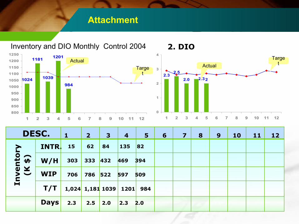
Attachment
Inventory and DIO Monthly Control 2004
Inven
tory
(K $
)
INTR.
W/H
WIP
T/T
DESC. 1 2 3 4 5 6 7 8 9 10 11 12
15 62 84 135 82
303 333 432 469 394
706 786 522 597 509
1,024 1,181 1039 1201 984
Days 2.3 2.5 2.0 2.3 2.0
2. DIO
1024
1181
1039
1201
984
800
850
900
950
1000
1050
1100
1150
1200
1250
1 2 3 4 5 6 7 8 9 10 11 12
2.32.5
2.0 22.3
0
1
2
3
4
1 2 3 4 5 6 7 8 9 10 11 12
Target
Actual TargetActual

Attachment
Inventory and DIO Budget Control 2004
Jan Feb Mar Apr May Jun Jul Aug Sep Oct Nov Dec
Sales Amount Target 12,060 12,176 12,569 12,256 12,290 12,322 12,432 12,879 12,874 12,197 10,740 11,551 146,346
Actual 13,784 13,668 15,892 15,388 15,423
In transit Target 45 45 45 41 41 41 40 40 40 40 40 40 42
Actual 15 62 84 135 82
W/house Target 372 372 372 365 365 365 365 365 365 325 325 325 357
Actual 303 333 432 469 394
WIP Target 695 695 695 672 672 672 672 672 672 665 665 665 676
Actual 706 786 522 597 509
Total Target 1,112 1,112 1,112 1,078 1,078 1,078 1,077 1,077 1,077 1,030 1,030 1,030 1,074
Actual 1,024 1,181 1,039 1,201 984
DIO Target 2.9 2.6 2.7 2.6 2.7 2.6 2.7 2.6 2.5 2.6 2.9 2.8 2.7
Actual 2.30 2.51 2.03 2.34 1.98
Avg/TotalDesc.2004

Attachment
1 2 3 4 5 6 7 8 9 10 11 12 1 2
In Transit 25 39 33 24 17 24 113 107 80 44 124 109 55 62 61
W I P 564 724 713 799 890 970 693 653 604 664 668 574 706 786 715
W/House 442 331 278 333 298 357 314 361 409 320 383 311 303 333 341
Total 1,031 1,094 1,024 1,156 1,205 1,351 1,120 1,121 1,093 1,029 1,175 994 1,064 1,181 1,117
Sales Amt 12,953 13,091 13,701 12,080 12,698 12,328 14,099 14,396 14,147 14,385 10,551 13,112 13,784 13,668 13,214
D I O 2.4675 2.3399 2.3169 2.8709 2.9412 3.2879 2.4632 2.4138 2.3186 2.2166 3.3403 2.3502 2.3936 2.5055 2.6205
MonthsavgDESC.
0
0.5
1
1.5
2
2.5
3
3.5
4
1 2 3 4 5 6 7 8 9 10 11 12 13 14 Avg
Material Inventory and DIO Control 2003 and 1 Q of 2004

Date Nov 24th , 2004
Process Technique GroupPrepared : Novi Muharam
Reduce LNG Usage
6σ
Ch
am
pio
n R
evie
wD
MA
IC R
ep
ort
Contents
1. Define Step 2. Measure Step3. Analysis Step4. Improvement5. Control


Background CIAM
D
LNG (Liquid Natural Gas) is source of energy for combustion process in F’ceUp to 3rd quarter LNG usage for exhaust furnace still higher, it’s about 5000 Nm3/day. This project have a purpose to decreasing LNG usage in furnace
4500
5000
Current Current Target Target
LNG Usage
Unit: (Nm3/day)
11%
How to do:
LNG & Air pressure systemAdjustment to find best ratio
Both of them.
Target Saving cost:
= (5000 –4500 )Nm3/day x 0.165 U$/Nm3 x 30 x 12= 500 Nm3/day x 0.165 x 30 x 12= 29,700 U$/Years29,700 U$/Years
OthersElec
tricO2N2LNG
0.00700.06050.12900.13090.1650 1.412.326.226.633.5
100.0 98.6 86.3 60.1 33.5
0.5
0.4
0.3
0.2
0.1
0.0
100
80
60
40
20
0
Defect
CountPercentCum %
Per
cent
Cou
nt
Energy Usage Price
Energy Unit Price (U$)

G/S
Load ExhP-pipe
Tip off B.B.D
Exhaust FurnaceZone #1 ~ #44
Unload
Robot
RobotControl Panel
-F/F C/V -CartIn
Out
KeepingZone
Up SlopeZone
Down Slope
Process MappingCIAM
D
CTQ Area : - LNG & Air Usage

LNG RatioUsage
Material LNG Pressure Ratio
Air Pressure Ratio
Machine TIC Temperature
RC Fan RPM Motor
Dumper Valve
Exh Blower Pressure
Big Y X1 X2 X3
D CIAM
Brainstormed Potential X List

GaR StdDev Study Var %Study Var
Source (SD) (5,15*SD) (%SV)
Total Gage R&R 0,009704 0,04998 1,40
Repeatability 0,002582 0,01330 0,37
Reproducibility 0,009354 0,04817 1,35
Operator 0,002566 0,01321 0,37
Operator*Part 0,008995 0,04633 1,30
Part-To-Part 0,692590 3,56684 99,99
Total Variation 0,692658 3,56719 100,00
Gage name:Date of study:Reported by:Tolerance:Misc:
Exhaust F'Ce MeasurementOct 19th, 2005
Novi M
0-1,5
-1,0
-0,5
0,0
0,5 Eng'r Gi jo Maker 1 maker 2 PQC
Xbar Chart by Operator
Sa
mp
le M
ea
n
Mean=-0,5057UCL=-0,5032LCL=-0,5082
0
0,000
0,005
0,010 Eng'r Gi jo Maker 1 maker 2 PQC
R Chart by Operator
Sa
mp
le R
ang
eR=0,001333
UCL=0,004356
LCL=0
a b c d e f
-1,0
-0,5
0,0
0,5
Part
OperatorOperator*Part Interaction
Ave
rag
e
Eng'r Gijo_1Gijo_2Gijo_3
PQC
Eng'r Gijo Maker 1 maker 2 PQC
-1,0
-0,5
0,0
0,5
Oper
Response By Operator
a b c d e f
-1,0
-0,5
0,0
0,5
Part
Response By Part
%Contribution %Study Var
Gage R&R Repeat Reprod Part-to-Part
0
50
100
Components of Variation
Pe
rce
nt
Gage R&R (ANOVA) for Auto 14"
Gage R&R for Exhaust F’ce Line #1 Measurement
Gage R&RD CIA
M
Gage R&R <20%
Acceptable
Gage R&R <20%
Acceptable

1086420
USLLSL
Exhaust F'ce 14" Capa'
PPM Total
PPM > USL
PPM < LSL
PPM Total
PPM > USL
PPM < LSL
PPM Total
PPM > USL
PPM < LSL
Ppk
Z.LSL
Z.USL
Z.Bench
Cpm
Cpk
Z.LSL
Z.USLZ.Bench
StDev (Overall)
StDev (Within)
Sample N
Mean
LSL
Target
USL
137981.99
90265.06
47716.94
14111.87
11722.77
2389.10
81081.08
81081.08
0.00
0.45
1.67
1.34
1.09
*
0.76
2.82
2.272.19
1.66305
0.98276
37
5.27297
2.50000
*
7.50000
Exp. "Overall" PerformanceExp. "Within" PerformanceObserved PerformanceOverall Capability
Potential (Within) Capability
Process Data
Within
Overall
Capability Process
1 2 3 4 5 6
1.0
0.5
1.5
2.0
2.5
Z Sh
ift
Proc
ess
Con
trol
Good
Poor
Z stTechnology
GoodPoor
Block A
Block C
Block B
Block D
A : Poor control, inadequate technology B : Must control the process better, technology is fineC : Process control is good, inadequate technologyD : World class
Four Block Diagram
D CIAM

Regression Analysis: Press LNG versus TempThe regression equation is
Press LNG = 3.7 + 21.9 Temp
Predictor Coef SE Coef T P
Constant 3.75 36.18 0.10 0.918
Temp 21.934 6.556 3.35 0.002
S = 64.96 R-Sq = 24.2% R-Sq(adj) = 22.1%
Analysis of Variance
Source DF SS MS F PP
Regression 1 47242 47242 11.19 0.0020.002Residual Error 35 147702 4220
Total 36 194945
Analysis
Accept Ha
Fail to reject Ho
The p-value < 0.05, Fail to accept Ho, which demonstrate statistical significance (an equation with a “good” fit)
The p-value < 0.05, Fail to accept Ho, which demonstrate statistical significance (an equation with a “good” fit)
LNG Pressure
ManometerGauge
D CIMA
P-Value: 0.321A-Squared: 0.414
Anderson-Darling Normality Test
N: 37StDev: 1.65154Average: 5.27297
9.28.27.26.25.24.23.22.2
.999
.99
.95
.80
.50
.20
.05
.01
.001
Pro
bab
ility
Qty LNG
Normal Probability Plot
Analysis of Temp furnace with result has significant effect to Pressure LNG
Hypothesis Analysis :Ho : Temperature furnace has no significant effect to LNG PressureHa : Temperature furnace has significant effect to LNG Pressure
Hypothesis Analysis :Ho : Temperature furnace has no significant effect to LNG PressureHa : Temperature furnace has significant effect to LNG Pressure

0 100 200 300 400 500 600 700 800 900
95% Confidence Intervals for Sigmas
Bartlett's Test
Test Statistic: 3.282
P-Value : 0.858
Levene's Test
Test Statistic: 2.096
P-Value : 0.131
Factor Levels
7575757575757575757575757575757575757575757575757575
0.1 0.2 0.5 0.6 1.7 2.0 3.0 4.0 5.0 6.0 6.8 7.0 7.3 8.0 9.0 9.1 9.3 9.811.011.611.812.012.913.514.214.6
Test for Equal Variances for LNG Ratio
One-way ANOVA: Air Press, Press LNG, TempAnalysis of Variance
Source DF SS MS F PP
Factor 2 1769458 884729 118.10 0.0000.000
Error 108 809084 7492
Total 110 2578542
Individual 95% CIs For Mean
Based on Pooled St Dev
Level N Mean StDev --+---------+---------+---------+----
Air Pres 37 424.73 73.53 (-*--)
Press LN 37 117.00 73.04 (--*--)
Temp 2 37 297.54 108.32 (--*--)
--+---------+---------+---------+----
Pooled StDev = 86.55 100 200 300 400
Tem
p
LNG
Pre
ss
Air
Pre
s
600
500
400
300
200
100
0
Boxplots of Air Press - Temp
(means are indicated by solid circles)
Analysis D CIM
A
Analysis of Temp furnace with result has significant effect to LNG & Air press
Hypothesis Analysis :Ho : Temperature furnace has no significant effect to LNG & Air PressureHa : Temperature furnace has significant effect to LNG & Air Pressure
Hypothesis Analysis :Ho : Temperature furnace has no significant effect to LNG & Air PressureHa : Temperature furnace has significant effect to LNG & Air Pressure

Regression Analysis: LNG Press versus RPM Motor The regression equation is
RPM = 1448 + 0.0344 LNG Press
Predictor Coef SE Coef T P
Constant 1448.00 5.02 288.20 0.000
LNG press 0.03440 0.01568 2.19 0.035
S = 8.711 R-Sq = 12.1% R-Sq(adj) = 9.6%
Analysis of Variance
Source DF SS MS F PP
Regression 1 365.11 365.11 4.81 0.0350.035Residual Error 35 2655.97 75.88
Total 36 3021.08
RC Fan Rotation
Analysis
Accept Ha
Fail to reject Ho
D CIMA
P-Value: 0.097A-Squared: 0.624
Anderson-Darling Normality Test
N: 37StDev: 19.1748Average: 1462.22
14901480147014601450144014301420
.999
.99
.95
.80
.50
.20
.05
.01
.001
Pro
bab
ility
RPM
Normal Probability Plot
Analysis of RPM motor with result has significant effect to Pressure LNG
Hypothesis Analysis :Ho : RPM motor has no significant effect to LNG PressureHa : RPM motor has significant effect to LNG Pressure
Hypothesis Analysis :Ho : RPM motor has no significant effect to LNG PressureHa : RPM motor has significant effect to LNG Pressure
The p-value < 0.05, Fail to accept Ho, which demonstrate statistical significance (an equation with a “good” fit)
The p-value < 0.05, Fail to accept Ho, which demonstrate statistical significance (an equation with a “good” fit)

Analysis
Regression Analysis: LNG Press Versus Air Blower The regression equation is
Air Blower = 475 - 0.169 LNG Press
Predictor Coef SE Coef T P
Constant 474.97 35.14 13.52 0.000
Air Blower -0.1689 0.1111 -1.52 0.138
S = 72.23 R-Sq = 6.2% R-Sq(adj) = 3.5%
Analysis of Variance
Source DF SS MS F PP
Regression 1 12044 12044 2.31 0.1380.138Residual Error 35 182604 5217
Total 36 194647
Exhaust F’ceBlower
Fail to accept Ha
Reject Ho
D CIMA
Average: 424.730StDev: 73.5314N: 37
Anderson-Darling Normality TestA-Squared: 0.200P-Value: 0.875
300 400 500 600
.001
.01
.05
.20
.50
.80
.95
.99
.999
Pro
bab
ility
Blower
Normal Probability Plot
Analysis of Air Blower with result has no significant effect to Pressure LNG
Hypothesis Analysis :Ho : RPM motor has significant effect to LNG PressureHa : RPM motor has no significant effect to LNG Pressure
Hypothesis Analysis :Ho : RPM motor has significant effect to LNG PressureHa : RPM motor has no significant effect to LNG Pressure

Regression Analysis: LNG Press versus DamperThe regression equation is
Damper = 428 - 0.43 LNG Press
Predictor Coef SE Coef T P
Constant 427.96 24.17 17.70 0.000
LNG press -0.425 2.745 -0.15 0.878
S = 74.55 R-Sq = 0.1% R-Sq(adj) = 0.0%
Analysis of Variance
Source DF SS MS F PP
Regression 1 133 133 0.02 0.8780.878Residual Error 35 194514 5558
Total 36 194647
Analysis
Damper
2001000-100
2
1
0
-1
-2
Nor
mal
Sco
re
Residual
Normal Probability Plot of the Residuals(response is Damper)
Fail to accept Ha
Reject Ho
D CIMA
Analysis of Damper with result has no significant effect to Pressure LNG
Hypothesis Analysis :Ho : RPM motor has significant effect to LNG PressureHa : RPM motor has no significant effect to LNG Pressure
Hypothesis Analysis :Ho : RPM motor has significant effect to LNG PressureHa : RPM motor has no significant effect to LNG Pressure

Analysis Resume D CIM
Select most effected factor in Regression and ANOVA with P value < 0.05Select most effected factor in Regression and ANOVA with P value < 0.05
Factor Detail Analysis Content Result ConclusionAnalysis Tool
Selected as vital fewP < 0.05
P < 0.05Selected as vital few
LNG Ratio Pressure and quantity adjustment For f’ce combustions
P < 0.05 Selected as vital few
Sample test for kind of air blower effect to gas ratio.
RPM MotorWith Gas
Heating result measurement insideFurnace.
P > 0.05
Not selected as vital few
Air & LNGPressure
Checking both of pressure Compare with temperature result
Air blowerWith Gas
Sample test for damper setting forEach position
P > 0.05Not selected as vital few
Damper With Gas
A
Regression
Regression
Regression
Regression
ANOVA

Bottle Neck D CIM
A
From furnace build until now, this furnace have never been done by Cleaning inside of f’ce
burner
Dilutionair
GasExhaustduct
To many Carbon (C)
To make efficiency, Need cleaningNeed cleaning inside of f’ce From Carbon (C) result of combustion.

Response Surface Regression: Result versus LNG Press, LNG Qty, ...The analysis was done using coded units.
Estimated Regression Coefficients for Result
Term Coef SE Coef T P
Constant 115.3 37.23 3.098 0.008
Block -25.0 17.44 -1.436 0.173
LNG Pres 108.1 18.39 5.878 0.000
LNG Qty -137.5 18.39 -7.478 0.000
AIR Pres -79.2 18.39 -4.310 0.001
RPM 3.9 18.39 0.213 0.834
LNG Pres*LNG Pres 2.4 17.20 0.142 0.889
LNG Qty*LNG Qty 78.6 17.20 4.568 0.000
AIR Pres*AIR Pres 26.9 17.20 1.566 0.140
RPM*RPM -10.3 17.20 -0.600 0.558
LNG Pres*LNG Qty -76.0 22.52 -3.375 0.005
LNG Pres*AIR Pres -51.5 22.52 -2.287 0.038
LNG Pres*RPM 3.5 22.52 0.155 0.879
LNG Qty*AIR Pres 39.2 22.52 1.743 0.103
LNG Qty*RPM -2.5 22.52 -0.111 0.913
AIR Pres*RPM -1.7 22.52 -0.078 0.93
S = 90.08 R-Sq = 91.7% R-Sq(adj) = 82.8%
Analysis of Variance for Result
Source DF Seq SS Adj SS Adj MS F P
Blocks 1 16733 16733 16733 2.06 0.173
Regression 14 1238887 1238887 88492 10.91 0.000
Linear 4 885220 885220 221305 27.27 0.000
Square 4 193821 193821 48455 5.97 0.005
Interaction 6 159846 159846 26641 3.28 0.031
Residual Error 14 113594 113594 8114
Lack-of-Fit 10 113594 113594 11359 * *
Pure Error 4 0 0 0
Improvement
The Improve phase identifies a solution and confirms that the proposed solution will meet or exceed the improvement goals of the project.
D CAMI

10
-1005
0
ratio0
500
100
1000
200 3000
400
Result
500LNG Press
Surface Plot of Result
Hold values: AIR Pres: 452.5 RPM: 1459.0
Improvement
Optimum condition when:
-LNG pressure 60.5 mmH2O-Ratio of gas 4.5-Air Pressure 452.5 mmH2O-RPM Motor 1459 rpm
Optimum condition when:
-LNG pressure 60.5 mmH2O-Ratio of gas 4.5-Air Pressure 452.5 mmH2O-RPM Motor 1459 rpm
D CAMI

D CAM
Improvement
7.56.55.54.53.52.5
USLLSL
Exhaust F'ce 14" Capability
PPM Total
PPM > USL
PPM < LSL
PPM Total
PPM > USL
PPM < LSL
PPM Total
PPM > USL
PPM < LSL
Ppk
Z.LSL
Z.USL
Z.Bench
Cpm
Cpk
Z.LSL
Z.USL
Z.Bench
StDev (Overall)
StDev (Within)
Sample N
Mean
LSL
Target
USL
1.71
0.00
1.71
0.07
0.00
0.07
0.00
0.00
0.00
1.55
4.64
6.12
4.64
*
1.76
5.27
6.94
5.27
0.464622
0.409704
37
4.65757
2.50000
*
7.50000
Exp. "Overall" PerformanceExp. "Within" PerformanceObserved PerformanceOverall Capability
Potential (Within) Capability
Process Data
Within
Overall
1 2 3 4 5 6
1.0
0.5
1.5
2.0
2.5
Z Sh
ift
Proc
ess
Con
trol
Good
Poor
Z stTechnology
GoodPoor
Block A
Block C
Block B
Block D
Four Block Diagram
I

4500
5000
Current Current Target Target
LNG Usage
Unit: (Nm3/day)
8%
D CAM
Improvement
I
4600
Result Result
92%92% Cost Saving:= (5000 – 4600 )Nm3/day x 0.165 U$/Nm3 x 30 x 12= 400 Nm3/day x 0.165 x 30 x 12
= 23,760 U$/years23,760 U$/years
Improvement Result

Control Plan
Control
Item Period Gauge Method Chart Type PIC
LNG PressEach Zone
Weekly DigitalManometer
Use check sheet Xbar - R PQCLeader exh
Air PressEach Zone
Weekly DigitalManometer
Use check sheet Xbar - R PQCLeader exh
LNG metercontrol
Daily Visual Use check sheet Xbar - R Leader exh
RPM Motor
Weekly Tachometer Use check sheet Xbar - R PQC
D IAMC

Process standard changes:
D IAM
Control
F’ceControl
LNG MeterDaily check
RecordData
F’ceControl
LNG MeterDaily check
RecordData
LNG & AIR PressWeekly check
Standard RecordData
Setting GasRatio
OK
NG
RecordData
Process Control
Weekly check sheet for Gas measurement
Standard:
-LNG pressure 60.5 ± 10 mmH2O-Ratio of gas 4.5-Air Pressure 452.5 ± 50 mmH2O
Standard:
-LNG pressure 60.5 ± 10 mmH2O-Ratio of gas 4.5-Air Pressure 452.5 ± 50 mmH2O
PIC: Leader Exh
PIC: PQC Exh
Before Before After After
C
PIC: Leader Exh