six-year review 3 technical support document for long … · six-year review 3 technical support...
TRANSCRIPT

Six-Year Review 3 Technical Support Document for Long-Term 2 Enhanced
Surface Water Treatment Rule

Office of Water (4607M) EPA-810-R-16-011 December 2016 www.epa.gov/safewater

Disclaimer
This document is not a regulation. It is not legally enforceable, and does not confer legal rights or impose legal obligations on any party, including EPA, states, or the regulated community. While EPA has made every effort to ensure the accuracy of any references to statutory or regulatory requirements, the obligations of the interested stakeholders are determined by statutes, regulations or other legally binding requirements, not this document. In the event of a conflict between the information in this document and any statute or regulation, this document would not be controlling.

This page intentionally left blank.

Six-Year Review 3 i December 2016 Technical Support Document for LT2
Table of Contents
Appendices .................................................................................................................................... iv
List of Exhibits ...............................................................................................................................v
Acronyms ..................................................................................................................................... vii 1 Introduction ................................................................................................................. 1-1
1.1 Purpose of This Document ............................................................................................ 1-1
1.2 Brief History and Overview of the Six-Year Review and Retrospective Review of Existing Regulations ................................................................................................. 1-1
1.2.1 Six-Year Review ................................................................................................. 1-1
1.2.2 Retrospective Review of Existing Regulations .................................................. 1-2
1.3 Summary of the LT2 Regulatory Review Efforts ......................................................... 1-2
1.4 Other Six-Year Review 3 Efforts .................................................................................. 1-4
2 Review Protocol ........................................................................................................... 2-1
3 History of the Long Term 2 Enhanced Surface Water Treatment Rule ............... 3-1
3.1 Statutory Authority ........................................................................................................ 3-1
3.2 Summary of the Rule ..................................................................................................... 3-1
3.2.1 History of the LT2 Promulgation ....................................................................... 3-2
3.2.2 Monitoring and Treatment Requirements for Unfiltered Systems ..................... 3-9
3.2.3 Requirements for Existing Uncovered Finished Water Reservoirs .................. 3-10
3.2.4 Disinfection Profiling and Benchmarking Requirements ................................. 3-10
3.2.5 Implementation Timeline .................................................................................. 3-10
4 Health Effects Information ........................................................................................ 4-1
4.1 Cryptosporidium ............................................................................................................ 4-3
4.1.1 Infectivity ............................................................................................................ 4-4
4.1.2 Morbidity .......................................................................................................... 4-20
4.1.3 Mortality ........................................................................................................... 4-25
4.2 Giardia ........................................................................................................................ 4-28
4.3 Viruses ......................................................................................................................... 4-30
4.4 Other Pathogens .......................................................................................................... 4-31
4.4.1 Fungi ................................................................................................................. 4-31
4.4.2 Protozoa ............................................................................................................ 4-32
4.4.3 Bacteria ............................................................................................................. 4-32
4.5 Summary ..................................................................................................................... 4-35

Six-Year Review 3 ii December 2016 Technical Support Document for LT2
5 Cryptosporidium Analytical Methods Information .................................................. 5-1
5.1 Performance of Method 1623.1 ..................................................................................... 5-2
5.1.1 Single-Laboratory Side-by-Side Comparison of Method 1623 with Method 1623.1 .................................................................................................... 5-2
5.1.2 Four-Laboratory Side-by-Side Comparison of Method 1623 with Method 1623.1 ................................................................................................................. 5-4
5.1.3 Fourteen-Laboratory Method 1623.1 Validation Data ....................................... 5-5
5.1.4 Summary ............................................................................................................. 5-6
5.2 Other Cryptosporidium Detection Techniques and Suggested Improvements ............. 5-7
5.3 Analysis and Recoveries of Cryptosporidium Isolates ................................................. 5-9
5.4 Conclusion ..................................................................................................................... 5-9
6 Occurrence and Exposure Information .................................................................... 6-1
6.1 Cryptosporidium ............................................................................................................ 6-3
6.1.1 Summary of Round 1 Occurrence Data .............................................................. 6-3
6.1.2 Predictive Modeling for Round 2 ....................................................................... 6-9
6.2 E. coli Indicator to Predict Cryptosporidium Occurrence ........................................... 6-15
6.2.1 Background ....................................................................................................... 6-15
6.2.2 Data Cleaning Process ...................................................................................... 6-16
6.2.3 Analysis ............................................................................................................ 6-19
6.2.4 Results and Discussion ..................................................................................... 6-26
6.3 Cooccurrence of Cryptosporidium and Other Pathogens of Concern ......................... 6-31
6.3.1 Giardia and Cryptosporidium Cooccurrence from ICR Supplemental Survey Data ...................................................................................................... 6-31
6.4 Summary ..................................................................................................................... 6-35
7 LT2 Microbial Toolbox and Other Tools ................................................................. 7-1
7.1 Summary of Data on Toolbox Options and Treatment Credits .................................... 7-2
7.2 Treatment Technology Usage ....................................................................................... 7-7
7.3 Microbial Toolbox Tools .............................................................................................. 7-8
7.3.1 Watershed Control Program ............................................................................... 7-8
7.3.2 Alternative Source/Intake Management ........................................................... 7-12
7.3.3 Presedimentation Basin with Coagulation ........................................................ 7-13
7.3.4 Two-stage Lime Softening ............................................................................... 7-14
7.3.5 Bank Filtration .................................................................................................. 7-15
7.3.6 Combined Filter Performance ........................................................................... 7-18
7.3.7 Individual Filter Performance ........................................................................... 7-19

Six-Year Review 3 iii December 2016 Technical Support Document for LT2
7.3.8 Demonstration of Performance of Treatment Process(es) ................................ 7-20
7.3.9 Bag or Cartridge Filters .................................................................................... 7-22
7.3.10 Membrane Filtration ......................................................................................... 7-23
7.3.11 Second Stage Filtration ..................................................................................... 7-27
7.3.12 Slow Sand Filtration ......................................................................................... 7-28
7.3.13 Chlorine Dioxide .............................................................................................. 7-30
7.3.14 Ozone ................................................................................................................ 7-31
7.3.15 UV Disinfection ................................................................................................ 7-33
7.4 Summary ..................................................................................................................... 7-44
8 Uncovered Finished Water Reservoirs ..................................................................... 8-1
8.1 Background on the LT2 Uncovered Finished Water Reservoir Requirements ............. 8-1
8.2 Background on Uncovered Finished Water Reservoirs ................................................ 8-1
8.3 Summary of Information Supporting the LT2 Requirements ....................................... 8-2
8.4 Information Available Since the Promulgation of the LT2........................................... 8-3
8.4.1 Permanent Solutions Taken ................................................................................ 8-5
8.4.2 Effectiveness of Permanent Solutions ................................................................ 8-5
8.4.3 Temporary Solutions Taken ............................................................................... 8-5
8.4.4 Effectiveness of Temporary Solutions................................................................ 8-6
8.5 Implementation Issues Related to the LT2 Cover/Treat Requirements ........................ 8-6
9 References .................................................................................................................... 9-1

Six-Year Review 3 iv December 2016 Technical Support Document for LT2
Appendices
Appendix A: Data for Methods 1623 and 1623.1 Cryptosporidium Recoveries
Appendix B: Occurrence and Exposure
Appendix C: Toolbox Option Usage and Related Implementation Issues

Six-Year Review 3 v December 2016 Technical Support Document for LT2
List of Exhibits
2 Review Protocol
Exhibit 2.1 Six-Year Review Protocol Overview and Major Categories of Revise/Take No Action Outcomes ..................................................................... 2-2
3 History of the Long Term 2 Enhanced Surface Water Treatment Rule Exhibit 3.1 Bin Classifications and Treatment Requirements for Filtered Systems ............ 3-6 Exhibit 3.2 Microbial Toolbox Components for the LT2..................................................... 3-8 Exhibit 3.3 Implementation Timeline for the LT2 for Filtered Systems ............................ 3-11
4 Health Effects Information Exhibit 4.1 Characteristics of the LT2 EA Primary Model and Six Alternative
Models ................................................................................................................ 4-5 Exhibit 4.2 Dose Response Relation, as a Function of Dose and IgG Level ..................... 4-10 Exhibit 4.3 A: Dose Response Relations for the Four Isolates (TAMU, Iowa, UCP
and Moredun); B: Quantile Contours of the Predicted Dose Response Relation Generalized from the Four Curves in A; C: Low Dose Extrapolated Dose Response Relations for the Four Isolates ........................... 4-12
Exhibit 4.4 Best Fit Models and Optimized Parameter Values for Cryptosporidium Isolates (CAMRA) ............................................................................................ 4-13
Exhibit 4.5 Fitting Dose-Response Curves of Infection Probability for Healthy Adult Volunteers and Intake of Cryptosporidium Oocysts ........................................ 4-14
Exhibit 4.6 Cryptosporidium Outbreaks Associated with Drinking Water, by Year: Waterborne Disease and Outbreak Surveillance System, United States 2005–2010 (CDC, 2008; 2011; 2013; 2015a) .................................................. 4-24
Exhibit 4.7 Giardia Outbreaks Associated with Drinking Water, by Year: Waterborne Disease and Outbreak Surveillance System, United States 2005–2010 (CDC, 2011; 2013) ........................................................................ 4-29
5 Cryptosporidium Analytical Methods Information Exhibit 5.1 Observed Recovery at a Single Laboratory, Using One Source Water and
Three Artificial Matrices .................................................................................... 5-3 Exhibit 5.2 Observed Recovery at a Single Laboratory, Using Nine Source Waters .......... 5-4 Exhibit 5.3 Observed Recovery at Four Laboratories, Using Three Source Waters ............ 5-4 Exhibit 5.4 Method 1623.1 Validation Data for 14 Laboratories, Reagent Water; N =
56 ........................................................................................................................ 5-6 Exhibit 5.5 Method 1623.1 Validation Data for 14 Laboratories, Source Water; N =
53 ........................................................................................................................ 5-6 6 Occurrence and Exposure Information
Exhibit 6.1 System Size and Round 1 Sampling Schedule .................................................. 6-1 Exhibit 6.2 Cryptosporidium Round 1 Monitoring Participation ......................................... 6-5 Exhibit 6.3 Cryptosporidium Round 1 Summary Statistics.................................................. 6-5 Exhibit 6.4 Cryptosporidium Round 1 Summary Statistics by Plant ................................... 6-5 Exhibit 6.5 Cryptosporidium Round 1 Summary Statistics by Source Water Type ............ 6-6

Six-Year Review 3 vi December 2016 Technical Support Document for LT2
Exhibit 6.6 Binning Results for Filtered Systems ≥ 10,000 People ..................................... 6-7 Exhibit 6.7 Binning Results for Plants in Grandfathered Systems ≥ 10,000 People ............ 6-9 Exhibit 6.8 Modeled Round 2 Outcomes Using Method 1623, by Source Water Type .... 6-12 Exhibit 6.9 Modeled Round 2 Outcomes Using Method 1623.1, by Source Water
Type .................................................................................................................. 6-13 Exhibit 6.10 Modeled Round 2 Outcomes by Source Water Type and Method ................ 6-14 Exhibit 6.11 Plants in Bins 2–4 under Alternative Scenarios on Occurrence
Distribution ....................................................................................................... 6-15 Exhibit 6.12 Definition of Variables Used in Analysis ...................................................... 6-19 Exhibit 6.13 Criteria for Reservoirs and Lakes Using Original Cleaning Procedure ......... 6-20 Exhibit 6.14 Criteria for Rivers and Flowing Streams Using Original Cleaning
Procedure .......................................................................................................... 6-21 Exhibit 6.15 Criteria for All Samples Using Original Cleaning Procedure ....................... 6-22 Exhibit 6.16 Criteria for Reservoirs and Lakes Using Revised Cleaning Procedure ......... 6-23 Exhibit 6.17 Criteria for Rivers and Streams Using Revised Cleaning Procedure ............ 6-24 Exhibit 6.18 Criteria for All Samples Using Revised Cleaning Procedure ........................ 6-25 Exhibit 6.19 E. coli Trigger Analysis Results for Small Plants Using Original
Cleaning Procedures ......................................................................................... 6-27 Exhibit 6.20 E. coli Trigger Analysis Results for Small Plants Using Revised
Cleaning Procedures ......................................................................................... 6-28 Exhibit 6.21 2010 Trigger Analysis Results ....................................................................... 6-29 Exhibit 6.22 Percent Reduction in Plants Required to Monitor with Alternate Trigger
Levels ................................................................................................................ 6-30 Exhibit 6.23 Distribution of ICRSS Source Waters by System Size and Water Type ....... 6-31 Exhibit 6.24 ICRSS Summary Statistics for Cryptosporidium and Giardia ...................... 6-31 Exhibit 6.25 Scatterplot of Observed Mean Concentrations for 87 Source Waters ........... 6-32 Exhibit 6.26 Deviance Information Criterion Model Results ............................................. 6-33
7 LT2 Microbial Toolbox and Other Tools Exhibit 7.1 Summary of New Information on the LT2 Microbial Toolbox Options ........... 7-3 Exhibit 7.2 Comparative Effectiveness of Tools for Different Organisms .......................... 7-4 Exhibit 7.3 Microbial Toolbox Tool Usage .......................................................................... 7-8 Exhibit 7.4 Summary of UV Findings ................................................................................ 7-38
8 Uncovered Finished Water Reservoirs Exhibit 8.1 Systems with Remaining UCFWRs as of December 2015 ................................ 8-2

Six-Year Review 3 vii December 2016 Technical Support Document for LT2
Acronyms
AIDS Acquired Immunodeficiency Syndrome ASDWA Association of State Drinking Water Administrators AWOP Area-Wide Optimization Program AWWA American Water Works Association BAT Best Available Technology BCDPW Baltimore City Department of Public Works BF Bank Filtration CAMRA Center for Advanced Microbial Risk Assessment CCL Contaminant Candidate List CDC Centers for Disease Control and Prevention CFE Combined Filter Effluent CFSE Carboxyfluorescein Diacetate Succinimidyl Ester CFU Colony-Forming Units CT the product of the residual disinfectant concentration “C” in
milligrams/liter (mg/L) and contact time “T” in minutes CWRWS Central Wyoming Regional Water System DBP Disinfection Byproducts D/DBPR Disinfectants/Disinfection Byproducts Rule DCTS Data Collection and Tracking System DEC Decimal Elimination Capacity DIC Deviance Information Criterion DMS Dyed Microsphere DNA Deoxyribonucleic Acid DOC Dissolved Organic Carbon DOP Demonstration of Performance EA Economic Analysis EHEC Enterohemorrhagic E. coli EMC Event Mean Concentration EO Executive Order EPA United States Environmental Protection Agency FA Factor Analysis FAC Federal Advisory Committee FCV Feline Calicivirus FDM-MPN Focus Detection Method–Most-Probable-Number FPUD Fallbrook Public Utility District FR Federal Register FS River/Stream GAC Granular Activated Carbon gpm Gallons Per Minute GWUDI Ground Water Under the Direct Influence HEA Health Effects Assessment HESD Health Effects Support Document HPC Heterotrophic Plate Count ICR Information Collection Rule

Six-Year Review 3 viii December 2016 Technical Support Document for LT2
ICRSS Information Collection Rule Supplemental Survey ID50 Median Infective Dose IDEM Indiana Department of Environmental Management IESWTR Interim Enhanced Surface Water Treatment Rule IFA Immunofluorescent Antibody and Microscopy Assay IFE Individual Filter Effluent IgG Immunoglobulin G IMS Immunomagnetic Separation IRIS Integrated Risk Information System JAGS Just Another Gibbs Sampler LADWP Los Angeles Department of Water and Power LED Light Emitting Diode LP Low Pressure LPHO Low Pressure, High Output LR Lake/Reservoir LRV Log Removal Values LT1 Long Term 1 Enhanced Surface Water Treatment Rule LT2 Long Term 2 Enhanced Surface Water Treatment Rule MDBP Microbial and Disinfection Byproducts MAC Mycobacterium avium Complex MCL Maximum Contaminant Level MCLG Maximum Contaminant Level Goal MCMC Markov Chain Monte Carlo MDBK Madin-Darby Bovine Kidney MF Microfiltration mgd Millions of Gallons per Day mg/L Milligrams/Liter mL Milliliters MLE Maximum-Likelihood Estimation MP Medium Pressure MPA Microscopic Particulate Analysis MRAA Maximum Running Annual Average MRSA Methicillin-Resistant Staphylococcus Aureus NaHMP Sodium Hexametaphosphate NDWAC National Drinking Water Advisory Council NF Nanofiltration NOM Natural Organic Matter NPDWR National Primary Drinking Water Regulation NTU Nephelometric Turbidity Units NYCDEP New York City Department of Environmental Protection O&M Operations and Maintenance OPP Office of Pesticide Programs OW Office of Water PAC Powdered Activated Carbon PCB Pathogen Catchment Budget PCR Polymerase Chain Reaction

Six-Year Review 3 ix December 2016 Technical Support Document for LT2
PMA Propidium Monoazide POU Point-Of-Use PQL Practical Quantitation Limit PSL Polystyrene Latex PT Proficiency Testing PUV Pulsed UV PWS Public Water System PWSA Pittsburgh Water and Sewer Authority QA Quality Assurance QC Quality Control QMRA Quantitative Microbial Risk Assessment qPCR Quantitative PCR RAA Running Annual Average RED Reduction Equivalent Dose RMP Risk Mitigation Plan RNA Ribonucleic Acid RO Reverse Osmosis RNA Ribonucleic Acid rRNA Ribosomal Ribonucleic Acid RT-PCR Reverse Transcription-PCR SCADA Supervisory Control and Data Acquisition SDWA Safe Drinking Water Act SDWIS Safe Drinking Water Information System SPU Seattle Public Utilities SSRC Spores of Sulfite-Reducing Clostridia SWTR Surface Water Treatment Rule SYR1 Six-Year Review 1 SYR2 Six-Year Review 2 SYR3 Six-Year Review 3 TCR Total Coliform Rule THM Trihalomethane TNRS Tennessee River Sediment TOC Total Organic Carbon TPU Tacoma Public Utilities TSS Total Suspended Solids TT Treatment Technique UCFWR Uncovered Finished Water Reservoirs UF Ultrafiltration UPS Uninterruptible power supply USEPA United States Environmental Protection Agency UV Ultraviolet UVA Ultraviolet A UVDGM Ultraviolet Disinfection Guidance Manual WBDO Waterborne Disease Outbreaks WCP Watershed Control Program WHO World Health Organization

Six-Year Review 3 x December 2016 Technical Support Document for LT2
WTP Water Treatment Plant
Six-Year Review 3 1-1 December 2016 Technical Support Document for LT2
1 Introduction
1.1 Purpose of This Document
The purpose of this document is to present technical information the U.S. Environmental Protection Agency (EPA) analyzed as part of the ongoing Six-Year Review 3 (SYR3) of the Long Term 2 Enhanced Surface Water Treatment Rule (LT2) as well as the Retrospective Review of the LT2 under Executive Order 13563. The Agency used the information presented in this document to formulate its determination of whether it would consider any changes to the LT2.
This introduction provides an overview of Six-Year Review and Retrospective Review requirements, and a summary of the SYR3 and Retrospective Review of the LT2. The end of this introductory section presents a brief overview of the content of the remaining chapters in this document.
1.2 Brief History and Overview of the Six-Year Review and Retrospective Review of Existing Regulations
1.2.1 Six-Year Review
Section 1412(b)(9) of the 1996 Safe Drinking Water Act (SDWA) Amendments requires EPA to conduct a review of each existing National Primary Drinking Water Regulation (NPDWR) at least once every six years and revise each as appropriate. Additionally, the SDWA specifies that any revision of a NPDWR “shall maintain, or provide for greater, protection of the health of persons.” To date, EPA has completed two rounds of Six-Year Reviews, referred to as the Six-Year Review 1 (SYR1) and the Six-Year Review 2 (SYR2). The EPA Administrator signed the notice announcing the results of the SYR1 on July 11, 2003, and the notice was published in the Federal Register (FR) on July 18, 2003 (USEPA, 2003a). The EPA Administrator signed the notice announcing the results of the SYR2 on December 17, 2009, and the notice was published in the FR on March 29, 2010 (USEPA, 2010a).
A decision to revise an NPDWR starts a regulatory process that involves more detailed analyses concerning health effects, costs, benefits, contaminant occurrence and other topics. At any point in this process, EPA may find that regulatory revisions are not appropriate and may discontinue regulatory revision efforts. Review of that NPDWR would, however, remain part of future Six-Year Reviews. Similarly, a determination to “take no action at this time” means only that EPA does not believe that regulatory changes to a particular NPDWR are appropriate at the current time based on health effects, analytical methods, treatment data, ongoing scientific reviews, priority or other reasons. EPA may decide in future Six-Year Reviews that regulatory changes are appropriate (USEPA, 2009a).
Under the SYR1, EPA identified only the Total Coliform Rule (TCR) as a candidate NPDWR for revisions, while EPA identified four NPDWRs under the SYR2 as candidates for revision: acrylamide, epichlorohydrin, tetrachloroethylene and trichloroethylene.

Six-Year Review 3 1-2 December 2016 Technical Support Document for LT2
1.2.2 Retrospective Review of Existing Regulations
In August 2011, EPA published its final plan for conducting periodic retrospective reviews of existing regulations, prepared in response to Executive Order 13563. The order required each federal agency to develop a plan “consistent with law and its resources and regulatory priorities. Under the final plan, the Agency will periodically review its existing significant regulations to determine whether any such regulations should be modified, streamlined, expanded or repealed so as to make the Agency’s regulatory program more effective or less burdensome in achieving the regulatory objectives” (USEPA, 2011a). In its plan, EPA identified 35 regulations, including the LT2, for inclusion in the first round of retrospective reviews. The plan stated that, “EPA intends to evaluate effective and practical approaches that may maintain, or provide greater protection of, the water treated by public water systems (PWSs) and stored prior to distribution to consumers. EPA plans to conduct this review expeditiously to protect public health while considering innovations and flexibility as called for in Executive Order (EO) 13563.” (USEPA, 2011a)
This Agency-wide effort, separate from the SDWA Six-Year Review process, aims to better understand the impacts of its regulations and, as noted above, identify ways to improve and make them less burdensome.
EPA completed its detailed review of the LT2 and at this time believes that it is not a candidate for regulatory revision.
1.3 Summary of the LT2 Regulatory Review Efforts
As part of the LT2 regulatory review, EPA assessed and analyzed information presented in this document regarding health effects and risks, monitoring methods, occurrence, the use of E. coli as a screen for small systems, the microbial toolbox and uncovered finished water reservoirs (UCFWRs), to evaluate whether there are new or additional ways to manage risk while assuring equivalent or improved public health protection.
EPA has developed and implemented protocols for ensuring a systematic approach is taken to conduct each of the Six-Year Reviews. EPA carried out an initial assessment of the application of the current protocol to the LT2 SYR3; EPA presents its consideration of the Six-Year Review Protocol Decision Tree for the LT2 and explains how EPA mapped the protocol to this LT2 Technical Support Document in Chapter 2.
EPA provides in Chapter 3 a history of the development of the LT2, a summary of the LT2 requirements, and information on the statutory authority EPA used to develop the LT2.
EPA evaluated available information on Cryptosporidium and other pathogens of concern that could potentially be present in source waters and UCFWRs. As part of this analysis, EPA noted new information on Cryptosporidium species that have recently been linked to human infection as part of this analysis. EPA presents a more complete discussion of potential pathogens of concern and health effects in Chapter 4 of this document.
In January 2012 EPA published a revision to Method 1623, the method used to determine the source water occurrence of Cryptosporidium and Giardia. Method 1623.1 encompasses

Six-Year Review 3 1-3 December 2016 Technical Support Document for LT2
improvements to Method 1623 regarding separation of Cryptosporidium oocysts from extraneous material and the removal of interfering substances. Method 1623.1 has been shown to increase recovery efficiencies for Cryptosporidium oocysts in some complex sample matrices. As part of this review, EPA determined that the impact of Method 1623.1 was not sufficient to justify requiring systems to use this method, but that systems could use it for compliance with the additional source water monitoring (e.g., a second round required under the LT2). EPA also evaluated other methods for determining the occurrence of Cryptosporidium in water samples, including polymerase chain reaction (PCR) and cell culture methods. Because of concerns with these methods (e.g., cell culture would detect some, but not all Cryptosporidium species), EPA believes that the use of these methods for LT2 compliance could amount to backsliding, which the SDWA specifically prohibits (i.e., Section 1412(b)(9) requires that revisions maintain or provide for greater protection of health). EPA provides more detail on these analyses in Chapter 5 of this document.
EPA conducted analyses on the LT2 source water monitoring requirements, and the Cryptosporidium occurrence data collected during the first round of monitoring, to determine the value of proceeding with the second round. While the data generated by the first round of source water monitoring indicated a lower occurrence rate than EPA predicted when it promulgated the LT2, EPA believes there is value in conducting the second round of monitoring to capture temporal changes in source water Cryptosporidium occurrence. To support its determination of the value of the second round of monitoring, EPA developed predictions of the numbers of additional systems that would be assigned to treatment bins as a result of Round 2 monitoring. EPA provides more detail on these analyses in Chapter 6 of this document.
Systems serving 100,000 or more people are defined as Schedule 1 systems, while systems serving 50,000 to 99,999 people, and those serving 10,000 to 49,999 people are defined as Schedule 2 and Schedule 3 systems, respectively. EPA analyzed the Cryptosporidium and E. coli data collected by Schedule 1-3 systems during Round 1 monitoring to determine the usefulness of E. coli as a screen for Schedule 4 (small) systems, that is, to determine whether E. coli occurrence correlated with Cryptosporidium occurrence. EPA determined that E. coli is an effective screen for determining the need for Schedule 4 systems to conduct Cryptosporidium monitoring. As a result, EPA will continue to allow Schedule 4 systems to use E. coli as a screen for Cryptosporidium monitoring for the second round of LT2 monitoring. Where E. coli concentrations are below certain levels, Cryptosporidium monitoring will not be required for small systems. EPA provides more detail on this analysis in Chapter 6 of this document.
Based on the source water monitoring results, systems are placed into one of four categories of additional treatment requirement (i.e., bins). Systems in Bin 1 require no additional treatment beyond existing requirements. Systems in Bins 2, 3 or 4 select from a microbial toolbox of options for ensuring Cryptosporidium source protection and management, removal or inactivation. EPA reviewed and analyzed available information on the microbial toolbox tools and other risk mitigation strategies to determine the need to revise the toolbox credits awarded for the use of the tools, and to determine the need to change the tools available in the microbial toolbox. Based on this analysis, EPA determined that no changes are warranted to the credits awarded to the tools in the microbial toolbox, because limited data exists that would support any changes. Also, stakeholders identified and provided feedback to EPA on implementation issues related to some of the tools from the microbial toolbox. EPA believes there is enough flexibility

Six-Year Review 3 1-4 December 2016 Technical Support Document for LT2
in the microbial toolbox that changes to the available tools are not necessary to address these implementation concerns. EPA provides more detail on these analyses in Chapter 7 of this document.
The LT2 included disinfection profiling and benchmarking requirements that apply if a PWS proposes to make a significant change to its disinfection practice as it implements the Stage 2 Disinfection Byproducts Rule and the LT2. EPA analyzed new disinfection studies to inform a determination of whether existing CT (the product of the residual disinfectant concentration “C” in milligrams/liter (mg/L) and contact time “T” in minutes) tables are still protective. EPA provides a detailed discussion of the results and implications of these more recent studies in the Six-Year Review 3 Technical Support Document for Microbial Contaminant Regulations (USEPA, 2016a).
To review the UCFWR requirements of the LT2, EPA collected information related to the potential risks posed by UCFWRs, and measures taken to address those risks. EPA also received stakeholder feedback during a public meeting devoted to UCFWRs. Based on the available information, EPA was unable to identify any alternative risk mitigation measures that are as effective as the cover or treat requirements of the LT2. EPA also notes that many PWSs have already addressed their UCFWRs. As a result, EPA believes that the cover or treat requirements that pertain to UCFWRs continue to be appropriate. EPA provides more detail on these analyses in Chapter 8 of this document.
EPA held three public meetings as part of the LT2 regulatory review. On December 7, 2011, EPA hosted a public meeting to discuss improvements to the Cryptosporidium analytical method and to provide an update on the LT2’s source water monitoring results. The two main objectives of this meeting were: (1) to start the LT2 regulatory review process, and (2) to meet the recommendation of the microbial and disinfection byproducts (MDBP) federal advisory committee (FAC) to have public meetings following the first round of monitoring. On April 24, 2012, EPA hosted a second public meeting to discuss information that could inform the regulatory review of the LT2 UCFWR requirement. The main objectives of this meeting were to: (1) provide background information on the UCFWR requirement and discuss/solicit public input, (2) provide an overview of the SYR3 process, and (3) engage in a scientific and technical discussion on data and information related to occurrence of Cryptosporidium, Giardia, viruses and other pathogens/indicators in UCFWRs; perspectives on public health risks; strategies to control or remove contaminants in UCFWRs; and potential assessment. On November 15, 2012, EPA hosted a third public meeting to discuss the review process, monitoring, occurrence, binning and microbial toolbox information. Summaries of these three public meetings, along with presentations made during the meetings, are available at www.epa.gov/dwsixyearreview/review-lt2-rule . Findings from the meetings are also discussed in more detail in applicable chapters of this document.
1.4 Other Six-Year Review 3 Efforts
The SYR3 examines rules that address chemical contaminants/indicators, radiological contaminants, microbiological contaminants/indicators, disinfection byproducts (DBPs)/indicators and disinfectant residuals. In addition to the LT2, the specific regulations under review include the Chemical Phase Rules (Inorganic, Synthetic Organic and Volatile

Six-Year Review 3 1-5 December 2016 Technical Support Document for LT2
Organic Chemicals); the Surface Water Treatment Rule (SWTR); the Interim Enhanced Surface Water Treatment Rule (IESWTR); the Long Term 1 Enhanced Surface Water Treatment Rule (LT1); the Ground Water Rule; the Filter Backwash Recycling Rule; the Stage 1 Disinfectants/Disinfection Byproducts Rule (D/DBPR); and the Stage 2 D/DBPR. This document covers the review of only the LT2; the reviews of other regulations included within the SYR3 are described in separate documents.

Six-Year Review 3 2-1 December 2016 Technical Support Document for LT2
2 Review Protocol
This chapter provides an overview of the process the Agency used to review the National Primary Drinking Water Regulations (NPDWRs) discussed in the Six-Year Review 3. The protocol document, “EPA Protocol for the Third Review of Existing National Primary Drinking Water Regulations,” contains a detailed description of the process the Agency used to review the NPDWRs (USEPA, 2016b). The foundation of this protocol was developed for the Six-Year Review 1 based on the recommendations of the National Drinking Water Advisory Council (NDWAC) (2000). This Six-Year Review 3 process is very similar to the process implemented during the Six-Year Review 1 and the Six-Year Review 2, with some clarifications to the elements related to the review of NPDWRs included in the MDBP rules.
Exhibit 2.1 presents an overview of the Six-Year Review protocol and major categories of review outcomes. The protocol is broken down into a series of questions about whether there is new information for a contaminant that suggests it is appropriate to revise one or more of the NPDWRs. The two major outcomes of the detailed review are either:
(1) the NPDWR is not appropriate for revision and no action is necessary at this time, or
(2) the NPDWR is a candidate for revision. Individual regulatory provisions of NPDWRs that are evaluated as part of the Six-Year Review are: maximum contaminant level goals (MCLGs), maximum contaminant levels (MCLs), maximum residual disinfectant level goals (MRDLGs), maximum residual disinfectant levels (MRDLs), treatment techniques, other treatment technologies and regulatory requirements (e.g., monitoring). The MCL provisions are not applicable for evaluation of the microbial contaminants regulations which establish treatment technique requirements in lieu of MCLs. The MRDLG and MRDL provisions are only applicable for evaluation of the DBP rules as part of the Six-Year Review.
The review elements that EPA considered for each NPDWR during the Six-Year Review 3 include the following: initial review, health effects, analytical feasibility, occurrence and exposure, treatment feasibility, risk balancing, and other regulatory revisions. Further information about these review elements are described in the protocol document (USEPA, 2016b).

Six-Year Review 3 2-2 December 2016 Technical Support Document for LT2
Exhibit 2.1 Six-Year Review Protocol Overview and Major Categories of Revise/Take No Action Outcomes
Yes
No
New information to suggest possible changes (i.e., to an MCLG, MCL, Treatment Technique and/or
other regulatory revisions)?
Meaningful opportunity for health risk reduction for persons served by PWS and/or cost savings while maintaining/improving public health protection?
Outcome:No action at this time
Outcome:Candidate
for Revision
Data sufficient to supportregulatory revision?
No new information
Low priority - No meaningful opportunity
Data gaps/emerging information
Yes
No
Ongoing or planned HEAHealth effects assessment (HEA)
in process or planned? *
NPDWRs Under Review
Yes
No
Yes
No
NPDWR reviewed in recent or ongoing action?
No
Yes Regulatory action ongoingor recently completed
* Contaminants with an HEA in process that have an MCL based on practical quantitation limit and are greater than MCLG are passed to the next question to evaluate potential to revise the MCL.
Uncertain – emerginginformation
The Initial Review branch of the protocol identifies NPDWRs with recent or ongoing actions and excludes them from the review process to prevent duplicative agency efforts (USEPA, 2016b). The cutoff date for the NPDWRs reviewed under the SYR3 was August 2008. Based on the Initial Review, EPA excluded the Aircraft Drinking Water Rule, which was promulgated in 2009, and the Revised Total Coliform Rule (RTCR) (the revision of the 1989 TCR), which was promulgated in 2013. Further, since most of the 1989 Total Coliform Rule (TCR) requirements were replaced by the 2013 RTCR, the 1989 TCR was excluded from the Six-Year Review.
Six-Year Review 3 3-1 December 2016 Technical Support Document for LT2
3 History of the Long Term 2 Enhanced Surface Water Treatment Rule
This chapter provides a brief history of the statutory authority EPA used to develop the Long Term 2 Enhanced Surface Water Treatment Rule (LT2) and of the development of the LT2, as well as description of the regulatory requirements that are part of the LT2.
3.1 Statutory Authority
The 1974 Safe Drinking Water Act (SDWA) authorized EPA to protect public health by regulating the nation’s public drinking water supply. Although the SDWA was amended slightly in 1977, 1979 and 1980, the most significant changes occurred when the SDWA was reauthorized in 1986 and amended in 1996. To safeguard public health, the 1986 amendments required EPA to set maximum contaminant level goals (MCLGs) and maximum contaminant levels (MCLs) for 83 contaminants. The 1986 amendments authorized EPA to require treatment techniques (TTs) instead of MCLs where appropriate. EPA was also required to establish regulations for disinfection of all public water supplies and to specify filtration requirements for water systems that draw their water from surface sources (US EPA, 1991). The disinfection and filtration requirements were intended to protect the public from potential adverse health effects due to exposure to Giardia lamblia, viruses, Legionella, heterotrophic bacteria and other pathogens that would be removed by those TTs.
3.2 Summary of the Rule
EPA convened the Stage 2 MDBP federal advisory committee (FAC) in March 1999 to evaluate new information and develop recommendations for the LT2 and the Stage 2 Disinfectants/Disinfection Byproducts Rule (Stage 2 D/DBPR). The FAC was comprised of representatives from EPA, state and local public health and regulatory agencies, local elected officials, Indian Tribes, drinking water suppliers, chemical and equipment manufacturers, and public interest groups. The FAC members signed an Agreement in Principle in September 2000 (USEPA, 2000) stating consensus recommendations of the group. For the LT2, the Committee recommended the following:
(1) Supplemental risk-targeted Cryptosporidium treatment by filtered public water systems (PWSs) with higher source water contaminant levels as shown by monitoring results,
(2) Cryptosporidium inactivation by all unfiltered PWSs, which must meet overall treatment requirements using a minimum of two disinfectants,
(3) A toolbox of treatment and control processes for PWSs to comply with Cryptosporidium treatment requirements,
(4) Reduced monitoring burden for small filtered PWSs, (5) Future monitoring to confirm or revise source water quality assessments, and (6) Development of guidance for ultraviolet (UV) disinfection and other toolbox
components.
Cover or treat existing uncovered finished water reservoirs (UCFWRs) or implement risk mitigation plans (RMPs).

Six-Year Review 3 3-2 December 2016 Technical Support Document for LT2
The primary intent of the LT2 is to supplement existing microbial treatment requirements for systems where additional public health protection is needed due to elevated source water Cryptosporidium concentrations. The LT2 requires filtered systems to monitor their source water for Cryptosporidium and/or Escherichia coli during two different rounds of monitoring. Each round of monitoring lasts one to two years, depending on system size. Systems must conduct a second round of monitoring to determine if source water conditions changed significantly.
Larger systems (those serving at least 10,000 people) are required to conduct their second round of monitoring six years after submitting their bin calculation, approximately 6 ½ years after completing their initial round of monitoring. Filtered systems serving fewer than 10,000 people may have as many as eight years after completing their first round to begin their second round of source water monitoring. While larger systems must monitor their source water for Cryptosporidium, smaller systems (those serving fewer than 10,000 people) can monitor for E. coli first; if their E. coli levels exceed established thresholds, the smaller systems must then conduct Cryptosporidium monitoring. Systems may opt out of the source water monitoring requirements of the LT2 if they provide 5.5-log Cryptosporidium inactivation or removal. Based on the Cryptosporidium results, filtered systems must meet one of four levels of treatment for Cryptosporidium (with the first level requiring no additional treatment). Unfiltered systems must also monitor for Cryptosporidium; as with filtered systems the duration of each round of monitoring depends on system size. All unfiltered systems must achieve 2-log (99 percent) or 3-log (99.9 percent) Cryptosporidium inactivation, depending on their source water Cryptosporidium levels. The LT2 also requires systems with UCFWRs either to cover the reservoirs or provide additional treatment to the water exiting the reservoir. The LT2’s provisions are described in more detail below. The first round of source water monitoring is complete. The second round began in 2015.
Most of the requirements in the final LT2 reflect consensus recommendations from the Stage 2 MDBP FAC. However, EPA did not include provisions for RMPs for UCFWRs in the final LT2 because EPA determined (after reviewing public comments on the Proposed LT2 (USEPA, 2003b)) that an RMP would not provide equivalent public health protection to covering or treating the UCFWRs. Consequently, an RMP would not meet the statutory provision for a TT to prevent adverse health effects from pathogens like Giardia and Cryptosporidium to the extent feasible (SDWA section 1412(b)(7)(A)).
3.2.1 History of the LT2 Promulgation
EPA promulgated the final LT2 requirements on January 5, 2006.1 The LT2 built upon the Interim Enhanced Surface Water Treatment Rule (IESWTR) and the Long Term 1 Enhanced Surface Water Treatment Rule (LT1) by improving control of microbial pathogens, specifically the contaminant Cryptosporidium.2 The LT2, in conjunction with the Stage 2 D/DBPR,3 addresses the trade-off between competing risks that are posed by the simultaneous control of microbial pathogens and DBPs. The disinfectants commonly used to kill microorganisms react
1 LT2 (USEPA, 2006a). 2 IESWTR (USEPA, 1998), LT1 (USEPA, 2002). 3 Stage 2 D/DBPR (USEPA, 2006b).

Six-Year Review 3 3-3 December 2016 Technical Support Document for LT2
with naturally occurring organic and inorganic matter in source water, forming DBPs that present potential risks for cancer and reproductive and developmental health effects. In order to balance the risks posed by DBPs and microbial pathogens, and to make it easier for water systems to comply with both rules, EPA promulgated the LT2 concurrently with the Stage 2 D/DBPR. The LT2 applies to all PWSs (i.e., 15 service connections or 25 people served for at least 60 days per year) that use surface water or ground water under the direct influence of surface water (GWUDI) as a source.
3.2.1.1 Monitoring and Treatment Requirements for Filtered Systems
Under the LT2, systems serving 10,000 or more people were required to first monitor source water Cryptosporidium concentrations. The required level of source protection, removal or inactivation increases for systems in higher bins (i.e., increasing source water concentrations of Cryptosporidium).
The LT2 includes source water monitoring and bin classification exemptions for all filtered systems that provided, or will provide, 5.5-log treatment4 for Cryptosporidium by the date on which they are required to comply with additional Cryptosporidium treatment requirements. To meet the requirement for 5.5-log treatment, systems using conventional treatment, diatomaceous earth filtration or slow sand filtration must provide 2.5-log additional treatment beyond what they are assumed to currently provide, and systems using direct filtration must provide 3-log additional treatment. The requirements for 5.5 log treatment for those systems using alternative filtration technologies are determined by the state.
3.2.1.2 Initial Monitoring for Bin Classification—Systems Serving at Least 10,000 People5
Schedule 1-3 filtered systems were required to monitor their raw water sources for Cryptosporidium at each plant at least once per month for a minimum of two years beginning October 2006.6 Bin classification was based on one of the following:
• The highest 12-month running annual average (RAA) Cryptosporidium concentration (in oocysts per liter) if samples were taken monthly (24 samples total), or;
• The 2-year mean Cryptosporidium concentration. The facility could conduct monitoring twice per month for 24 months (48 samples total) or perform additional sampling and
4 The term “log removal” is used when the contaminant is eliminated by way of filtration; “log inactivation” is used when oocysts are killed by disinfection. The term “log treatment” encompasses both removal and inactivation, and is used to reflect the fact that under the LT2, treatment will be achieved using a combination of filtration, disinfection, and other non-traditional methods. 5The monitoring and treatment requirements for wholesale systems—i.e., those that sell water only to other systems—was dependent on the population served by the largest system in the combined distribution system. 6 The largest systems (serving 100,000 people or more) were required to begin monitoring October 2006. Systems serving 50,000 to 99,999 people were required to begin monitoring April 2007; systems serving 10,000 to 49,999 people were required to begin monitoring April 2008.

Six-Year Review 3 3-4 December 2016 Technical Support Document for LT2
include these results in the calculation of the mean, but the additional samples had to be evenly distributed over the 2-year monitoring period.
Cryptosporidium analysis was required to be conducted in accordance with EPA Method 1622/1623 using a sample volume of at least 10 liters.7 Samples were also required to be analyzed for E. coli and turbidity. EPA analyzed the E. coli and turbidity data to determine whether the data could help predict Cryptosporidium occurrence.
Systems with historical Cryptosporidium data that were equivalent in sample number, frequency and quality to data required under the LT2 Round 1 monitoring were allowed to use these data to determine bin classification in lieu of conducting additional Cryptosporidium monitoring, if the state approved the use of these data. Systems with less than two years of Cryptosporidium data were also allowed to grandfather their data and collect less than two full years of Cryptosporidium samples, if the data they had previously collected were equivalent in sample number, frequency and quality of data required under the LT2 Round 1 monitoring, represented the months when Round 1 sampling would not be taking place, and the state approved the use of the data. These are referred to as grandfathered data.
Systems and their laboratories submitted monitoring results to EPA by entering the data into an EPA database known as Data Collection and Tracking System (DCTS). Systems that grandfathered data were not required to use DCTS, and additional systems also submitted their data directly to the primacy agency, not through DCTS. EPA prepared quarterly files containing the data and delivered those files to the states/primacy agencies via their EPA regional offices. Systems were responsible for determining their bin placements and reporting their bins to their states/primacy agencies for approval within six months of completing their monitoring.
7 Systems must meet all requirements of the analytical methods for Cryptosporidium, which include analysis of two matrix spiked samples.
Six-Year Review 3 3-5 December 2016 Technical Support Document for LT2
3.2.1.3 Initial Monitoring for Bin Classification—Systems Serving Fewer than 10,000 People
The LT2 required small filtered systems (defined as Schedule 4) to conduct E. coli source water monitoring starting in October 2008, two years after the first large systems initiated source water Cryptosporidium monitoring. EPA delayed the small system monitoring schedule to allow incorporation of information on E. coli and turbidity collected by the medium and large systems into the monitoring requirements as necessary. Based on the Schedule 1-3 systems’ data analyses, EPA determined that turbidity does not appear to be very informative regarding Cryptosporidium occurrence, whereas E. coli does have merit in this regard. EPA provides more discussion in Chapter 6, Section 6.2 of this document. Therefore, Schedule 4 systems conducted one year of biweekly E. coli source water monitoring and were required to conduct Cryptosporidium monitoring if E. coli concentrations exceeded the following levels8:
• An annual mean concentration greater than 10 E. coli per 100 milliliters (mL) for lake and reservoir source waters,
• An annual mean concentration greater than 50 E. coli per 100 mL for flowing stream source waters, or
• Alternative trigger levels of 100 E. coli per 100 mL for source waters drawing from both lakes/reservoirs and flowing streams.9
EPA assumed that filtered Schedule 4 systems that did not exceed these levels had a Cryptosporidium concentration of less than 0.075 oocysts/L, and these systems were placed in Bin 1 (Exhibit 3.1). Schedule 4 systems that exceeded the E. coli levels mentioned above were required to conduct Cryptosporidium monitoring twice per month for a 1-year period or monthly for a 2-year period, beginning in April 2010, six months after the conclusion of E. coli monitoring. Bin classification for Schedule 4 systems conducting Cryptosporidium monitoring was determined by the highest 12-month RAA.
Schedule 4 systems and their laboratories submitted monitoring data to EPA by either submitting the data directly to their state/primacy agency or by entering the data into DCTS. Systems were responsible for determining their bin placements and reporting their bins to their state/primacy agency for approval within six months of completing their monitoring.
3.2.1.4 Bins and Treatment Requirements—All System Sizes
Exhibit 3.1 presents the bins for filtered systems according to the type of treatment already in place. Systems must meet Cryptosporidium treatment requirements by using one or a combination of the treatment options in the “microbial toolbox,” or by demonstrating performance equivalent to, or exceeding the required treatment. The LT2 requires systems to
8 Small systems were also required to conduct Cryptosporidium monitoring if they failed to conduct E. coli monitoring or if they elected to proceed directly to Cryptosporidium monitoring. 9 Alternative trigger levels were identified in USEPA (2010b).

Six-Year Review 3 3-6 December 2016 Technical Support Document for LT2
meet the treatment requirements associated with their bin placement within three years after first being assigned to a bin. States/primacy agencies may grant systems a 2-year extension to comply if capital investments are necessary. Systems must report to the state their bin placement within six months of completing their source water monitoring.
Exhibit 3.1 Bin Classifications and Treatment Requirements for Filtered Systems
If your source
And if you use the following filtration treatment in full compliance with existing regulations, then your additional treatment requirements are . . .
water Cryptosporidium
concentration (oocysts/L) is . . .
Your bin classification
is . . . Conventional
Filtration Direct
Filtration
Slow Sand or Diatomaceous
Earth Filtration
Alternative Filtration
Technologies
< 0.075 1
No additional treatment
No additional treatment
No additional treatment
No additional treatment
> 0.075 and < 1.0 2 1-log
treatment 1.5-log
treatment 1-log treatment As determined
by the state1
> 1.0 and < 3.0 32 2-log
treatment 2.5-log
treatment 2-log treatment As determined
by the state3
> 3.0 42 2.5-log
treatment 3-log
treatment 2.5-log
treatment As determined by the state4
Notes: 1) Total Cryptosporidium treatment must be at least 4.0-log.
2) Systems must achieve at least 1-log of the required treatment using ozone, chlorine dioxide, UV light, membranes, bag/cartridge filters or bank filtration (BF).
3) Total Cryptosporidium treatment must be at least 5.0-log.
4) Total Cryptosporidium treatment must be at least 5.5-log.
The total Cryptosporidium treatment required for systems in Bins 2, 3 and 4 is 4.0-log, 5.0-log and 5.5-log, respectively. EPA based the additional treatment requirements in Exhibit 3.1 on information obtained after EPA promulgated the IESWTR and the LT1 that indicates that conventional, slow sand and diatomaceous earth filtration plants in compliance with the IESWTR or the LT1 achieve an average of 3-log removal of Cryptosporidium across all plants. The IESWTR and the LT1 require systems to achieve 2-log removal; EPA based this requirement on the information on the minimum removal expected from these types of filtration (USEPA, 2006a). Therefore, systems with conventional, slow sand and diatomaceous earth filtration plants will require an additional 1.0- to 2.5-log treatment to meet the total treatment requirement, depending on the bin in which the systems are placed.
In the LT2 EPA determined that direct filtration plants achieve an average 2.5-log removal of Cryptosporidium (USEPA, 2006a). The removal is less than the removal in conventional filtration because direct filtration lacks a sedimentation process. Consequently, under the LT2, direct filtration plants in Bins 2-4 must provide 0.5-log more in additional treatment than conventional plants to meet the total Cryptosporidium treatment requirement.

Six-Year Review 3 3-7 December 2016 Technical Support Document for LT2
3.2.1.5 Microbial Toolbox for Meeting Additional Treatment Requirements
To meet the Cryptosporidium treatment requirements for the bin in which they are classified, filtered systems select from a “toolbox” of treatment or management options. Exhibit 3.2 lists the treatment and management strategies comprising the microbial toolbox, and Chapter 7 includes a discussion of these strategies in more detail. EPA prescribed each option in the toolbox with a certain amount of log treatment credit, which systems can apply toward their total treatment requirements. [Systems do not get the log credit automatically when they install these technologies; systems must show that they are meeting certain operational or performance criteria specific to each technology in order to receive credit.] Log treatment credit under the existing rules (e.g., the IESWTR and the LT1) works in a similar process. Systems already using ozone, chlorine dioxide, UV light or membranes, in addition to conventional treatment prior to the promulgation of the LT2, can receive credit for those technologies toward meeting bin requirements if they meet the LT2 criteria for the chosen technology. Systems currently using chorine and/or chloramines do not receive credits for these disinfectants under the LT2 because `

Six-Year Review 3 3-8 December 2016 Technical Support Document for LT2
Exhibit 3.2 Microbial Toolbox Components for the LT210
Toolbox Option Log Treatment Credit
Source Toolbox Components
Watershed control program 0.5
Alternative source/intake management
No presumptive credit. Systems may conduct simultaneous monitoring for treatment bin classification at alternative intake locations or under alternative intake management strategies.1
Pre-Filtration Toolbox Components
Presedimentation basin with coagulation
0.5
Two-stage lime softening 0.5
BF 0.5 or 1.0, depending on setback
Treatment Performance Toolbox Components
Combined filter performance 0.5
Individual filter performance 1.0
Demonstration of performance (DOP) State approved2
Additional Filtration Toolbox Components
Bag filters 2.0 as individual and 2.5 for two in series
Cartridge filters 2.0 as individual and 2.5 for two in series
Membrane filtration As demonstrated3
Second stage filtration 0.5
Slow sand filters 2.5
Inactivation Toolbox Components
Chlorine dioxide As demonstrated4
Ozone As demonstrated4
UV As demonstrated2 Notes:
1) Exhibit 3.3 of the Microbial Toolbox Guidance Manual contains additional information (USEPA, 2010c).
2) The state must approve the method used to demonstrate performance and must approve the log credit claimed by the system.
3) EPA based the credit for membrane filtration and UV on the results of equipment-specific testing.
4) EPA based the credit for chlorine dioxide and ozone on CT values achieved (CT is the product of disinfectant concentration and contact time).

Six-Year Review 3 3-9 December 2016 Technical Support Document for LT2
3.2.1.6 Reassessment and Future Monitoring
Six years after initial bin classification, systems must conduct a second round of monitoring to reassess source water conditions for bin assignments. Systems that provide a total of 5.5-log treatment for Cryptosporidium are not subject to future monitoring if they provide that treatment by the compliance date for Round 1 monitoring.
For those Schedule 1-3 systems not providing a total of 5.5-log treatment for Cryptosporidium, the second round of monitoring began no later than October 2016.11 For Schedule 4 systems, the second round of monitoring begins no later than October 2019.
In addition to the second round of monitoring described above, in their primacy application the state/primacy agency will describe how they will assess any significant changes in the watershed and source water as part of the sanitary survey process.
3.2.2 Monitoring and Treatment Requirements for Unfiltered Systems
Prior to the LT2 promulgation, unfiltered systems were required to address Cryptosporidium through their watershed control plans but did not have specific log inactivation requirements for Cryptosporidium. The LT2 established new treatment requirements for unfiltered systems, except that unfiltered systems that already have 3-log Cryptosporidium treatment in place prior to the compliance date are exempt from source water monitoring and additional Cryptosporidium inactivation requirements.
Unfiltered Schedule 1-3 systems were required to monitor Cryptosporidium in their source water monthly for at least two years, and unfiltered Schedule 4 systems had to monitor Cryptosporidium twice a month for 12 months or monthly for 24 months. All unfiltered systems determined their treatment requirements based on the arithmetic mean Cryptosporidium concentration. Systems with an average Cryptosporidium concentration of less than or equal to 0.01 oocysts/L must provide 2-log Cryptosporidium inactivation. If their average concentration is greater than 0.01 oocysts/L, they must provide 3-log inactivation.
EPA based the monitoring for unfiltered systems on the same schedule as monitoring for filtered systems, although unfiltered systems are not required to monitor E. coli or turbidity. As with the filtered systems, unfiltered systems must conduct a second round of Cryptosporidium monitoring six years after the initial bin assignment, unless they provide 3-log treatment for Cryptosporidium.
In addition to the new Cryptosporidium inactivation requirements, the LT2 requires unfiltered systems to continue to meet the filtration avoidance criteria under the 1989 Surface Water Treatment Rule (SWTR) and to continue to provide inactivation for Giardia and viruses.
10 In order for a water system to receive Cryptosporidium treatment credit for using a toolbox option, the system must comply with the operational, monitoring, and reporting requirements associated with the toolbox option that EPA established in the LT2 or by the primacy agency. 11 Schedule 1 systems began monitoring no later than April 2015. Schedule 2 systems began monitoring no later than October 2015; Schedule 3 systems began monitoring no later than October 2016.

Six-Year Review 3 3-10 December 2016 Technical Support Document for LT2
Systems must meet the overall inactivation requirements (i.e., 4-log virus, 3-log Giardia, and 2- or 3-log Cryptosporidium) using a minimum of two disinfectants. Additionally, each of two disinfectants must meet the total inactivation for one of the three pathogens. For example, a system could use UV to inactivate 2-log of Cryptosporidium and Giardia and use chlorine to inactivate 4-log of viruses and 1-log of Giardia.
3.2.3 Requirements for Existing Uncovered Finished Water Reservoirs
The LT2 builds on the IESWTR and the LT1, which require covers only for new finished water reservoirs. The LT2 established requirements for all systems with existing UCFWRs. Systems must either cover the reservoir or treat the water exiting the reservoir to the distribution system to achieve 2-log Cryptosporidium, 3-log Giardia lamblia and 4-log virus inactivation.
3.2.4 Disinfection Profiling and Benchmarking Requirements
A disinfection profile is a graphical representation of a system’s level of Giardia and virus inactivation measured during the course of one or more year(s). A benchmark is the lowest monthly average of microbial inactivation during the disinfection profile period. The LT2 includes disinfection profiling and benchmarking requirements that apply if a public water system (PWS) proposes to make a significant change to its disinfection practice as it implements the Stage 2 Disinfectants and Disinfection Byproducts Rule and the LT2 [40 CFR 141.708–709]. The LT2 defines a significant change as a change to the point of disinfection, a change in the disinfectant used, a change to the disinfection process or any other modification that the state identifies as significant.
EPA developed profiling and benchmarking requirements under the Interim Enhanced Surface Water Treatment Rule and the LT1 and extended the requirements to the LT2 to address similar risk-balancing tradeoffs between the control of microbial pathogens and disinfection byproducts (DBPs).
The LT2 requires these systems to prepare a disinfection profile that characterizes current levels of Giardia lamblia and virus inactivation throughout the plant over the course of one year. Prior to making the change, the system must calculate a benchmark and consult with the state regarding how the proposed change will affect the current disinfection level.
A detailed discussion of disinfection profiling and benchmarking is described in the Six-Year Review 3 (SYR3) Technical Support Document for Microbial Contaminant Regulations (USEPA, 2016a).
3.2.5 Implementation Timeline
Exhibit 3.3 shows the timeline of the LT2 activities for filtered systems as described in previous sections. The schedule for monitoring and compliance with treatment requirements differs by population served.

Six-Year Review 3 3-11 December 2016 Technical Support Document for LT2
Exhibit 3.3 Implementation Timeline for the LT2 for Filtered Systems

Six-Year Review 3 4-1 December 2016 Technical Support Document for LT2
4 Health Effects Information
EPA uses the Health Effects Branch of the Six-Year Review Protocol primarily to assess whether scientific information suggests a potential for revision of a maximum contaminant level goal (MCLG) under an existing rule. MCLGs are nonenforceable health goals set at a level at which no known or anticipated adverse health effects occur and which allow an adequate margin of safety.
The 1996 Safe Drinking Water Act (SDWA) amendments require special consideration of all sensitive populations (e.g., infants, children, pregnant women, elderly, individuals with a history of serious illness) in the development of drinking water regulations. In addition, EPA’s plan for Retrospective Review of Existing Regulations criteria for review outlines consideration of effect of the regulation on children. New studies about the effect of Cryptosporidium on children further support EPA’s conclusion in the Long Term 2 Enhanced Surface Water Treatment Rule (LT2) (USEPA, 2006a) that Cryptosporidium may have a disproportionate effect on children. Since the promulgation of the LT2, there is additional evidence that asymptomatic Cryptosporidium infection in children can lead to reduced and delayed growth. The LT2 states that while Cryptosporidium may have a disproportionate effect on children, available data were not adequate to distinctly assess the health risk for children resulting from Cryptosporidium-contaminated drinking water. No new data have been found to allow for that assessment. Therefore, the approach to assessing children’s risk as part of the Six-Year Review 3 (SYR3) process would be the same as used to support the LT2 (USEPA, 2006a). In assessing risk to children when evaluating regulatory alternatives for the LT2, EPA assumed the same risk for children as for the population as a whole. This is consistent with Executive Order (EO) 13045 “Protection of Children from Environmental Health Risks and Safety Risks.” The Agency explained in the LT2 preamble why the planned regulation is preferable to other potentially effective and reasonably feasible alternatives considered by EPA. EPA concluded that result of the LT2 will be a reduction in the risk of illness for the entire population, including children (USEPA, 2006a).
Under the Six-Year Review Protocol Health Effects Branch, EPA also considers whether the peer-reviewed literature findings include health effects that are significantly different from those considered previously that could lead to a nomination for a new agency HEA.
With respect to the LT2, EPA did not establish any new MCLGs when the LT2 was promulgated. However, EPA established MCLGs for several pathogenic microorganisms under various preceding versions of the Surface Water Treatment Rules that led up to the LT2. Under the 1989 Surface Water Treatment Rule (SWTR), EPA established MCLGs of zero for Giardia lamblia12, viruses and Legionella (USEPA, 1989a). At the same time, EPA promulgated the related Total Coliform Rule (TCR) (USEPA, 1989b) which established an MCLG of zero for all coliform bacteria, including fecal coliforms and Escherichia coli specifically. Under the 1998
12 The current preferred taxonomic name is Giardia duodenalis, with Giardia lamblia and Giardia intestinalis as synonymous names. However, Giardia lamblia was the name used to establish the MCLG in 1989. Elsewhere in this document this pathogen will be referred to as Giardia spp. or simply Giardia unless discussing information on an individual species.

Six-Year Review 3 4-2 December 2016 Technical Support Document for LT2
Interim Enhanced Surface Water Treatment Rule (USEPA, 1998), EPA established an MCLG of zero for Cryptosporidium.
EPA established treatment technique (TT) requirements for all the surface water treatment rules including the LT2 in lieu of finished water maximum contaminant levels (MCLs) for the pathogens being addressed by the MCLGs noted earlier in this section of the document. EPA used a TT for the LT2 because it recognized that it was not economically or technologically feasible to determine the level of Cryptosporidium in finished water for the purpose of compliance with a finished water standard (i.e., MCL) (USEPA, 2006a). This limitation has been recognized since the time of the original 1989 SWTR where EPA similarly concluded that a TT rule was needed for Giardia, Legionella and virus noting that: (1) the only analytical methods which are available require levels of expertise that many utility personnel do not have; (2) analysis by independent laboratories is generally very expensive; and (3) systems would have to monitor inordinately large and frequent samples of water to ensure that the occurrence of these pathogens is not of health risk significance (e.g., failure to detect Giardia in one or a few samples provides no assurance that Giardia do not occur at significant levels in the water supply).
One specific focus of the LT2 was to require the use of risk-targeted additional TTs for all public water systems (PWSs) that use surface water sources, including ground water under the direct influence of surface water (GWUDI), and have relatively high Cryptosporidium levels in their source waters. In addition, the LT2 also addressed specific treatment requirements for uncovered finished water reservoirs (UCFWRs), for which the health effect concerns extend beyond Cryptosporidium to other pathogens.
Because the LT2 uses a TT requirement rather than an MCL, EPA also considered new health effects information under the TT Analysis Branch of the Six-Year Review Protocol to help inform the decision as to whether a meaningful opportunity exists for any TT revisions to lower health risks.
EPA has organized this health effects information chapter around the pathogens that the LT2 and its predecessor surface water treatment rules are designed to address:
• 4.1 Cryptosporidium, • 4.2 Giardia, • 4.3 Viruses, and • 4.4 Other pathogens.
Because the risk-based TT requirements of the LT2 focus primarily on Cryptosporidium risks associated with exposure from filtered and unfiltered systems, the bulk of the discussion presented in this chapter regarding new health effects information involves that pathogen. However, EPA also reviewed new information on other pathogens of concern to determine whether additional measures are warranted to provide public health protection from those pathogens, particularly in the context of the UCFWR components of the LT2.

Six-Year Review 3 4-3 December 2016 Technical Support Document for LT2
4.1 Cryptosporidium
The risk assessment for Cryptosporidium that EPA conducted in support of the LT2 was structured in accordance with EPA’s general framework for conducting health risk assessments for environmental contaminants.
The first two risk-assessment framework components are most concerned with health effects information, the subject of this chapter. The hazard identification component discussed in this chapter addresses the specific adverse health effects associated with Cryptosporidium, while the dose-response assessment addresses the relationship between the magnitude of exposure to Cryptosporidium and the likelihood of those adverse health effects occurring.
Because the critical adverse health effects associated with Cryptosporidium are well known—severe gastrointestinal illness that can in some cases be fatal, especially for certain susceptible subpopulations—EPA focused on gathering and reviewing new information concerning various elements of the dose-response assessment component of the Cryptosporidium health risk assessment for the LT2 effort rather than on the hazard identification component.
As described in detail in the LT2 Economic Analysis (EA) (USEPA, 2005a), the dose-response assessment model that was developed for Cryptosporidium to support the LT2 has three distinct parts:
• Infectivity: addresses the probability of an individual becoming infected given ingestion of one or more oocysts;
• Morbidity: addresses the probability of an infected individual becoming ill and experiencing the gastrointestinal illness symptoms of cryptosporidiosis, and;
• Mortality: addresses the probability of a case of cryptosporidiosis being fatal to an individual.
For this review of the LT2, EPA focused on the following key aspects of the dose-response assessment and the risk characterization:
• Are there additional human challenge studies that can also be used to parameterize the infectivity dose-response function?
• Are there studies suggesting alternative model forms for infectivity different from the exponential model used in the 2005 LT2 EA that EPA should consider?
• Are there studies or data suggesting alternative approaches to considering immunity in the exposed population for the dose-response modeling of infectivity?
• Are there studies or data that provide additional information on the assumption concerning the “v” ratio (the ratio of the fraction of infectious oocysts in the environment (numerator) to the fraction of infectious oocysts in doses tested in clinical challenge studies (denominator)) of infectious oocysts?

Six-Year Review 3 4-4 December 2016 Technical Support Document for LT2
• Are there studies or data that provide additional information on the estimates of the morbidity rate (risk of illness given an infection)?
• Are there studies or data that provide additional information on the estimates of mortality rate (risk of death given an illness)?
For this review effort, EPA conducted literature searches to identify published information relevant to Cryptosporidium infectivity, morbidity and mortality that has become available since EPA promulgated the LT2.
The following sections present and discuss the approach EPA used to characterize Cryptosporidium infectivity, morbidity and mortality at the time of the LT2 promulgation, as well as new information that has become available since that time that EPA could use to update the assessment of Cryptosporidium health risks for the Six-Year Review.
4.1.1 Infectivity
In the LT2 EA, EPA used several variations of a basic dose-response model for infectivity that were intended individually, and in combination, to reflect the uncertainty associated with modeling the probability of a Cryptosporidium infection occurring in humans given a dose (number of oocysts) ingested by an individual.
The basic dose-response model used for infectivity in the LT2 EA is the exponential model having the form:
PI = 1 – e –d r
where PI is the probability of an individual becoming infected given ingestion of a dose “d” of oocysts. The model parameter “r”, which is estimated from fitting the model to human challenge data, has a value between zero and one and is effectively a measure of the probability that an infectious organism that has been ingested will survive and cause an infection in the host.
At the time of the LT2 proposal in 2003, EPA used human challenge study data that were then available from three different C. parvum isolates (TAMU, Iowa and UCP) to parameterize the infectivity dose-response model. Following the proposal, EPA acquired data for two additional C. parvum isolates (Moredun and 16W), as well as for one C. hominis isolate (TU502). EPA used the human challenge data from these six isolates in a variety of ways to develop alternative infectivity models that were used as the primary model for the risk assessment, and as alternatives to capture the underlying uncertainty in the data and the model selections.
Exhibit 4.1 taken from the LT2 EA summarizes the key characteristics of those model variations. The models differ with respect to the model form (as noted above); the number and type of Cryptosporidium isolates used to estimate the r and, where used, the γ parameters for those models; the assumed distributional form characterizing the r parameter; and the underlying assumptions with respect to the source of variability in the r parameter obtained from the human challenge data, namely, organism variability or host variability.

Six-Year Review 3 4-5 December 2016 Technical Support Document for LT2
Exhibit 4.1 Characteristics of the LT2 EA Primary Model and Six Alternative Models
Model Data Sets Functional Form Distribution of r
Assumptions Mean Risk1
Primary Model (random selection from four models)
Two models use two studies; two models use three studies
PI = 1 - e –d r Two models use normal (logit); two models use t(3)-distribution
Assumes the four models are equally plausible; r distribution assumes organism variability
0.082
Alternative Model 1
6 studies PI = 1 - e –d r Normal (logit)
r distribution assumes organism variability
0.036
Alternative Model 2
6 studies PI = 1 - e –d r t(3)-distribution
r distribution assumes organism variability
0.046
Alternative Model 3
6 studies PI = 1 - e –d r Beta distribution
r distribution assumes organism variability
0.052
Alternative Model 4
6 studies PI = γ x (1 – e –d r) Beta distribution
r distribution assumes organism variability; additional parameter for information on host immunity
0.137
Alternative Model 5
6 studies PI = 1 - e –d r Beta distribution
r distribution assumes host variability
0.140
Alternative Model 6
6 studies PI = γ x (1 – e –d r) Beta distribution
r distribution assumes host variability; additional parameter for information on host immunity
1.105
Note: 1) Mean risk calculated from the distribution of r and γ values used as inputs for the dose-response model
(primary model reflects combination of all four components.)
EPA performed data analysis using a statistical model that addressed uncertainty due to limitations in the number of available isolates and subjects studied. The analysis treated the isolates as a random sample from a larger population of isolates potentially present in source waters (environmental samples). The model used the challenge study data to estimate the infectivity of these environmental isolates. Combining this information, the model predicts infectivity of an unknown environmental isolate, which serves as input to the benefits model. The environmental isolate accounts for uncertainty within each of the isolates and the uncertainty between those isolates.
The expected mean risk of infectivity (the dose response parameter (r)) in this case is equivalent to the probability that ingestion of a single organism will cause infection. It is not possible to know the true mean value of r, given the limitations in available data, variability between isolates, and the likelihood of unknown strains present in the environment. EPA derived the expected value of r from a distribution of r values that reflect the uncertainty within and variability among strains, including strains for which there are no data.
As indicated in Exhibit 4.1, the “primary model” EPA used in the LT2 EA was a composite of four models from which EPA selected outputs randomly in a simulation to capture uncertainty in the infectivity estimates. Specifically, two of the models had the form and assumptions of

Six-Year Review 3 4-6 December 2016 Technical Support Document for LT2
Alternative Model 1 and two had the form and assumptions of Alternative Model 2 as shown in Exhibit 4.1. In one set of Model 1 and Model 2, the r parameters were based on human challenge results for two isolates (Iowa and TAMU) while the other set of Model 1 and 2 used results for three isolates (Iowa, TAMU and UCP). Again, EPA combined these four model variations to form the single primary model that was used in the LT2 EA.
In addition to the primary model, EPA also separately modeled infectivity using the six model forms and assumptions indicated in Exhibit 4.1, and in those cases using the human challenge data from all six of the isolates identified previously.
(For a more detailed discussion of the LT2 EA infectivity modeling, the reader is referred to Chapter 5 and Appendix N of the LT2 EA.)
One important aspect of the infectivity modeling to note is that in the modeling procedures addressed earlier in this section of the document to arrive at the estimates of the model parameters r and γ, EPA assumed that all of the oocysts ingested by the individuals in the human challenge studies were “viable and infectious.” This is not, however, assumed to be the case with respect to ingestions of oocysts in drinking water derived from environmental sources. Therefore, in the application of the infectivity dose response models to estimating infectivity in the population exposed from drinking water, EPA included an additional parameter in the model as shown below for the basic exponential model form:
PI = 1 – e – d v r
where “v” is the fraction of environmental oocysts that are “viable and infectious”. EPA included this value in the modeling as a distribution reflecting uncertainty in the expected value for this parameter. The range of those values varied depending upon the dataset used for the environmental oocysts (15 to 25 percent for the Information Collection Rule (ICR) data, 30 to 50 percent for the Information Collection Rule Supplemental Survey (ICRSS) data) and based on the fraction of “empty” oocysts observed in those studies. [Note that v can also be viewed as a “viability fraction” where the numerator is the fraction of environmental oocysts considered to be viable and infectious, and the denominator the fraction in the human challenge studies considered to be viable and infectious which, as noted above, is assumed to be 1. This assumption is discussed further below.]

Six-Year Review 3 4-7 December 2016 Technical Support Document for LT2
For EPA’s LT2 review of new information relevant to the infectivity portion of the Cryptosporidium dose-response model, the Agency focused on three main elements:
• The review of new human challenge studies (including the role of immunity),
• The review of new quantitative dose-response model forms (also including the role of immunity), and
• The review of new information on oocyst viability studies.
4.1.1.1 Review of New Human Challenge Studies
A microbial human challenge study is the deliberate exposure of human volunteers to a range of doses of a microorganism to evaluate infectivity. The human challenge study data EPA evaluated and used in the LT2 EA included data from a total of six Cryptosporidium isolates. Those isolates included Iowa (DuPont et al., 1995; Okhuysen et al., 1999), TAMU (Okhuysen et al., 1999), UCP (Okhuysen et al., 1999), Moredun (Okhuysen et al., 2002), TU502 (Chappell et al., 2006) (note that this is an updated citation for the then-unpublished feeding study data for this C. hominis isolate) and 16W (the data for this C. parvum isolate have not been published in a peer-reviewed manuscript).
In the human challenge studies EPA used for the LT2 development, human volunteers who had low levels of pre-existing anti-Cryptosporidium immunoglobulin G (IgG) antibodies13 were initially challenged with Iowa, UCP, TAMU, TU502 and Moredun isolates. In these trials, the ID50s (the median infective dose) varied substantially, indicating potential differences in infectivity among these isolates (Okhuysen et al., 1999; Okhuysen et al., 2002). Nineteen of the 29 volunteers who had been challenged with the Iowa isolate were rechallenged after one year, with a single dose of 500 oocysts. Of these 19, infection was observed in 15 in the first challenge and no infection was observed in four. The rechallenge resulted in the same frequency of diarrhea symptoms as the first challenge, indicating a lack of protective immunity against infection and illness, although the number of oocysts shed by infected volunteers was lower than in the first challenge (Okhuysen et al., 1998). When the same Iowa isolate was tested in a different group of volunteers with and without pre-existing serum IgG to C. parvum, the ID50 was 14–20 fold higher in the volunteers with pre-existing IgG, and illness was significantly associated with the highest doses (DuPont et al., 1995; Chappell et al., 1999). Based on these observations, high IgG levels could indicate a recent Cryptosporidium infection and may be associated with a protective response, but with a likely duration of less than 12 months.
The literature review EPA conducted for the Six-Year Review revealed several new challenge studies published after the LT2, and one published prior to the LT2 but not explicitly considered previously. In this latter study, Chappell et al. (1999) evaluated the infectivity of C. parvum (Iowa strain) in healthy adults with pre-existing anti-C. parvum serum IgG. In this study, 17
13 IgG antibodies are associated primarily with the secondary immune response and are indicative of a past exposure to the antigen of interest and provide a potential measure of the extent and duration of immunity from subsequent exposures.

Six-Year Review 3 4-8 December 2016 Technical Support Document for LT2
healthy adults were challenged with 500–50,000 oocysts. Infection and diarrhea were associated with the higher challenge doses. The ID50 was 1,880 oocysts, >20-fold higher than in seronegative volunteers from previous challenge studies with this strain (DuPont et al., 1995; Okhuysen et al., 1999). In other words, it took a greater number of oocysts to produce an infection in adults with pre-existing anti-C. parvum serum IgG. Fecal oocysts were detected in only 7 of 13 individuals (54 percent) with clinical cryptosporidiosis, indicating that the host response may effectively decrease the number of oocysts produced. Subjects with the highest IgG levels prior to challenge had little to no increase in IgG following challenge, whereas volunteers with lower IgG levels showed significant postchallenge increases. This suggests that an upper limit of serum IgG was present in some subjects, while others were further stimulated by an additional exposure. These data imply that prior exposure to C. parvum may provide some protection from infection and illness.
Chappell et al. (2011) examined the infectivity of C. meleagridis in healthy adults. (Note that C. meleagridis was not among the species or isolates used in the LT2 risk assessment.) Five volunteers were challenged with 105 C. meleagridis oocysts and monitored during six weeks for fecal oocysts and clinical manifestations. All five volunteers had evidence of infection by either clinical or microbiological measures, or both. Four volunteers had diarrhea yielding an 80 percent illness rate. Three had detectable fecal oocysts. Two of the four volunteers with diarrhea had detectable oocysts, and two did not. One volunteer had no unformed stools or symptoms while shedding low, but detectable, numbers of oocysts. Fecal deoxyribonucleic acid (DNA) from two volunteers was amplified by using a polymerase chain reaction (PCR) specific for the Cryptosporidium small subunit ribosomal ribonucleic acid (rRNA) gene. Nucleotide sequence of these amplicons was diagnostic for C. meleagridis. All infections were self-limited and oocysts were cleared within 12 days of challenge. These studies establish that healthy adults can be infected and become ill from ingestion of C. meleagridis oocysts. These findings are consistent with a study that evaluated the epidemiology and symptoms of cryptosporidiosis patients in Sweden, reporting cases due to C. parvum (n=111), C. hominis (n=65), C. meleagridis (n=11), C. felis (n=2), C. chipmunk genotype I (n=2) and C. viatorum (n=2). That study also reported that clinical manifestations differed slightly by species with diarrhea lasting longer in C. parvum cases compared to C. hominis and C. meleagridis cases (Insulander et al., 2012). A similar finding was also reported in Ethiopia, where symptoms of diarrhea where longer in patients infected with C. parvum as compared with C. hominis (Adamu et al., 2014. PLOS Neg. Trop. Dis 8:e2831).
As part of an EPA research grant, Chappell et al. (2003) examined the potential for C. muris to infect healthy adults. (Note that C. muris was not among the species or isolates used in the LT2 risk assessment.) Each of six volunteers was challenged with 105 C. muris oocysts and monitored for six weeks for infection and/or illness. All six became infected, and two experienced a diarrheal illness. The number of total oocysts shed during the study ranged from 6.7 x 10⁶ to 4.1 x 10⁸, and was higher (mean = 2.8 x 10⁸) in volunteers with diarrhea than in asymptomatic shedders (mean = 4.4 x 10⁷). Follow-up fecal examinations at seven months postchallenge on five of the six volunteers revealed that three volunteers were still positive for fecal oocysts. These data establish the susceptibility of healthy humans to C. muris infection. C. muris illness was self-limiting in two cases and resulted in persistent, asymptomatic infections in three persons for seven months before treatment cleared the infection.

Six-Year Review 3 4-9 December 2016 Technical Support Document for LT2
Sheoran et al. (2012) conducted a challenge study with gnotobiotic piglets to investigate cross-protection from C. hominis and C. parvum. After ≥3 days of recovery from C. hominis infection, the piglets were completely protected against subsequent challenge with C. hominis but only partially against challenge with C. parvum, as compared with age-matched control animals challenged with either species. All C. hominis–C. parvum group piglets shed oocysts 3–4 days after the challenge infection, whereas none of the C. hominis–C. hominis group shed any oocysts for the duration of the experiment. However, total oocyst counts of the null–C. parvum group (range, 98–225) were significantly higher than that of the C. hominis–C. parvum group. Based on these results the authors conclude that C. hominis-specific immunity was sufficient to completely protect against challenge with the same species but insufficient to provide the same level of protection against C. parvum.
4.1.1.2 Review of Key Dose Response Modeling Studies
EPA evaluated the key dose response modeling studies to determine if data exist that suggest EPA should consider revisions to the TT requirements of the LT2. Teunis et al. (2002a) reevaluated three of the Cryptosporidium isolates (Iowa, TAMU, UCP) that had been evaluated previously in challenge studies (DuPont et al., 1995; Okhuysen et al., 1999) and that had been reported to have different ID50s. Those previous results, the findings of which are based on serologically negative healthy volunteers, indicated substantial variation in their infectivity for humans with ID50s of 1,042 for UCP, 87 for the Iowa isolate and 9 for TAMU. In this investigation, both within- and between-isolate variability were considered. The results indicate that in these controlled conditions there is substantial variation in infectivity among these isolates, although greater heterogeneity may exist among unspecified environmental strains. This analysis yields a wider estimate of the posterior range of the infection risk, reflecting additional uncertainty. Based on this work, starting from a discrete number of pathogens, the resultant dose response model would be a binomial model with Beta heterogeneity (a Beta-binomial model) both within and between isolates.
Teunis et al. (2002b) adapted the hit theory model of microbial infection to incorporate covariables, characterizing the immune status of the susceptible host. The probability of any single oocyst in the inoculum causing infection appears to depend on pre-existing IgG levels. Since these can be measured in human populations, the authors concluded that the IgG-dependence of the dose-response relation can be used to assess the distribution of susceptibility to infection and illness by Cryptosporidium and could be easily applied in quantitative risk analysis.
There are several possible ways to account for immunity and/or differential susceptibility to infection in a quantitative microbial risk assessment (QMRA). One possibility suggested by Teunis et al. (2002b) and implemented in the World Health Organization (WHO) risk assessment for Cryptosporidium (2009) is to use individual IgG levels as a proxy for susceptibility to partly control for host variation in the general population. To incorporate a covariable like IgG level into the dose response relationship, one can make the dose response relationship dependent on that covariable. One approach would be to use a logistic relation nested into the exponential dose response model. For example, when data from the two studies with the Iowa isolate are combined, one has data on infection in subjects with a wide range of IgG levels. Thus, one possibility would be to fit the IgG-dependent dose response model results in a function for the

Six-Year Review 3 4-10 December 2016 Technical Support Document for LT2
probability of infection which shows that there is a protective effect associated with high levels of (prechallenge) IgG. When such a model is applied to subjects with high pre-existing IgG, there is decreasing infectivity with increasing IgG levels. Exhibit 4.2 shows the results from one such dose response relation, as a function of dose and IgG level (WHO, 2009). Exhibit 3.2 shows the maximum likelihood dose response relationship fit to both low and high IgG data, a function of dose and pre-existing IgG levels.
Exhibit 4.2 Dose Response Relation, as a Function of Dose and IgG Level
Englehardt and Swartout (2004) present a hierarchical predictive population dose-response Bayesian assessment for C. parvum for the infection endpoint. The authors used available data on the infectivity of three isolates of C. parvum (Iowa, TAMU and UCP) to adjust, by bootstrap analysis, for sensitive and antibody-positive subpopulations not proportionately represented in the data. The authors used the diverse mean infectivities of the isolates to obtain a predictive distribution for population infectivity, which was used to obtain the predictive population dose-response function. The result is a distribution of unconditional probability of infection, based on available dose-response information. Information includes theoretical and empirical evidence for the conditional beta-Poisson parametric dose-response function. Results indicate that a dose of 6× 10⁻⁶ oocysts per exposure, and assuming 365 exposures per year, corresponds to 10−4 infections per person per year. By comparison, the corresponding estimate of daily oocyst exposure resulting in a 10-4 annual infection risk using the “best estimates” of parameter values and exposure assumptions in the EA would be 1.5 x 10⁻⁵ to 7.6 x 10⁻⁶oocysts, where EPA used factors of 0.2 and 0.4, respectively, to reflect the fraction of oocysts that are viable and infectious. Englehardt and Swartout (2004) did not include consideration of viability in their analysis, implying a factor of 1.0. If this factor is set to1.0 in the EPA EA analysis, the daily oocyst intake corresponding to an annual infection risk of 10-4 would be 3.0 x 10⁻⁶.
WHO conducted a risk assessment for Cryptosporidium in drinking water (WHO, 2009) that used the results from the Cryptosporidium human challenge studies conducted at the University of Texas as the basis for their dose response relationship (Okhuysen et al., 1999; Okhuysen et al., 2002). Four isolates (Iowa, TAMU, UCP and Moredun) formed the basis of this work for

Six-Year Review 3 4-11 December 2016 Technical Support Document for LT2
individuals with and without pre-existing C. parvum IgG (Chappell et al., 1999). To obtain a dose-response relationship, WHO analyzed the infection data as a binary (yes/no) response, with the single hit model for microbial infection. The modeling approach is a two-level model, the lower hierarchical level representing variation in isolates, and the upper level representing variation among hosts. WHO used the beta-Poisson dose response model with the parameters (α ,β) taken from (joint) distributions, describing the “between isolates” variation. This approach generalizes the heterogeneous infectivity to the “group” level for isolates, treating the four data sets as an n=4 sample from the presumed population of environmental oocysts. The distribution may be interpreted as the frequency distribution for dose response relations from the oocysts. Sampling from this distribution produces a predictive dose response relation which covers a wide range of infectivities. However, even with this wide range of infectivity, at low doses the exposure part of dose response relations becomes dominant: overall uncertainty in the predicted infectivity may be about 10-fold (Exhibit 4.3).

Six-Year Review 3 4-12 December 2016 Technical Support Document for LT2
Exhibit 4.3 A: Dose Response Relations for the Four Isolates (TAMU, Iowa, UCP and Moredun); B: Quantile Contours of the Predicted Dose Response Relation
Generalized from the Four Curves in A; C: Low Dose Extrapolated Dose Response Relations for the Four Isolates
C
The Center for Advanced Microbial Risk Assessment (CAMRA) has a QMRA wiki for current quantitative information and knowledge developed for QMRA (Enger, 2013). The dose response section of that wiki contains CAMRA’s summary and analysis for C. parvum and C. hominis dose response. Although this wiki has not been subject to the same peer review as manuscripts, the wiki provides best fit models and optimized parameter values (obtained via 10,000 bootstrap iterations) for the five published Cryptosporidium isolates. EPA presents a summary of those results in Exhibit 4.4.

Six-Year Review 3 4-13 December 2016 Technical Support Document for LT2
Exhibit 4.4 Best Fit Models and Optimized Parameter Values for Cryptosporidium Isolates (CAMRA)
Strain Best Fit Model Optimized Parameter(s)
ID50 Probability of Infection for Dose=1 Oocyst
TAMU Exponential k =0.0572 12.1 0.06 TU502 beta-Poisson α=0.27 N50=16.8 16.8 0.14 Iowa Exponential k =0.00419 165 0.004 Moredun beta-Poisson α=0.114 N50=455 455 0.07 UCP beta-Poisson α=0.145 N50=179 179 0.07
Mitchell-Blackwood (2010) used a Bayesian hierarchical modeling approach to evaluate the dose-response relationship for six Cryptosporidium strains (based on the human challenge study data from the University of Texas). The results indicated that individual (nonhierarchical) models rank highest and that three of the data sets (UCP, TU502 and Moredun) do not fit the exponential model. Moreover, maximum-likelihood estimation (MLE) estimates indicated that goodness of fit was achieved by the beta-Poisson model for all data sets, but the improvement over the exponential model was not statistically significant for the data sets that fit the exponential-based model. Parameter value estimates for TAMU, UCP and Iowa were consistent with the MLE and hierarchical models reported by Messner et al. (2001). All individual models generally agree with the MLE estimates for the Cryptosporidium spp. isolates.
An et al. (2011) conducted a quantitative health risk assessment of Cryptosporidium in rivers in China that included an extensive and novel dose response assessment based on five strains of Cryptosporidium. They indicate that Cryptosporidium infectivity modeling has typically neglected the virulence differential among strains. Different strains of pathogens normally coexist in the environment, and some strains may not be known, making it impossible to predict the infection rate of each strain using its specific dose-response curve. To solve this problem, An et al. used mixed dose-response curves to predict the infection rate at a specific dose by bootstrap resampling, based on all of the existing dose-response patterns of different Cryptosporidium strains. Thus, the authors assumed that all strains agreed with the same dose-response curve type, with their specific parameter values (α and β) based on the difference in virulence, with the curve type selected according to the model selection criteria. They fitted the dose-response curves using the beta-Poisson function and obtained curves for different isolates based on groups of parameters (α, β), which they resampled using the bootstrapping method with 2000 trials. EPA provides the resultant dose response relationship graphically in Exhibit 4.5. The red circles in Exhibit 3.5 indicate the observed dataset from the healthy adult volunteers, and the blue lines represent the bootstrap predicted curves. The bootstrap resampling curves converge with decreasing Cryptosporidium dose, which agrees well with previously published dose-response relationships for individual strains.

Six-Year Review 3 4-14 December 2016 Technical Support Document for LT2
Exhibit 4.5 Fitting Dose-Response Curves of Infection Probability for Healthy Adult Volunteers and Intake of Cryptosporidium Oocysts
The following discussion uses the probability that ingestion of a single organism will cause infection (equivalent to the dose response parameter (r) from an exponential distribution or the expected value of r) to compare the relative level of infectivity used in the LT2 risk assessment to other recently published assessments.
As summarized in this section, An et al. (2011) conducted a quantitative risk assessment of Cryptosporidium in rivers in China that included an extensive dose response assessment based on five strains of Cryptosporidium. To address the issue of multiple Cryptosporidium strains potentially present in the environment they used mixed beta-Poisson dose-response curves based on bootstrap resampling. Inspection of the resultant family of dose response curves (Exhibit 4.5) indicates that the range of probabilities that a single organism will cause infection (that is, where the log dose in Exhibit 4.5 is 0) is similar to mean values from the LT2 analysis, although the resultant range of r values (probability of infection due to ingestion of one oocyst) is narrower than the range used in the LT2 analysis.
Cummins et al. (2010) employed a quantitative Monte Carlo simulation model to evaluate the annual risk of infection from Cryptosporidium in tap water in Ireland. In this study an exponential dose response model was used with an r = 0.00526 (as reported in Pouillot et al. (2004)). This relative level of probability that a single organism will cause infection is lower than that used in the LT2 EA, and corresponds more closely to the infectivity of the TAMU isolate than an unknown mixture of isolates based on all of the available challenge study data.
The CAMRA QMRA wiki contains a summary and analysis for C. parvum and C. hominis dose response. Comparing the optimized dose response relationships for each of five Cryptosporidium strains to the infectivity of the “environmental strains” used in the LT2 analysis indicates that the

Six-Year Review 3 4-15 December 2016 Technical Support Document for LT2
relative level of infectivity used in the LT2 is at the upper range of the infectivity for the optimized individual strains (range 0.004 to 0.14).
WHO conducted a risk assessment for Cryptosporidium in drinking water (WHO, 2009) using the results from the Cryptosporidium human challenge studies for four isolates (Iowa, TAMU, UCP and Moredun) as a basis. As summarized previously, the modeling approach was a two-level model, the lower hierarchical level representing variation in isolates, and the upper level representing variation among hosts. The beta-Poisson dose response model is used with the parameters (α ,β) taken from (joint) distributions, describing the “between isolates” variation. This approach generalizes the heterogeneous infectivity to the “group” level for isolates, treating the four data sets as an n=4 sample from the presumed population of environmental oocysts. This distribution produces a predictive dose response relation that covers a wide range of infectivities and appears to suggest substantial uncertainty, as also suggested by the LT2 dose response modeling. The median infectivity and associated uncertainty predicted by this modeling approach are similar to that suggested by the set of models employed in the LT2 assessment.
4.1.1.3 Review of New Studies on Viable and Infectious Oocysts
Johnson, Rochelle and their colleagues (Johnson et al., 2010; Rochelle et al., 2012) conducted a study to determine the prevalence of infectious Cryptosporidium in conventionally treated drinking water. The authors analyzed a total of 370 samples comprising 349,053 L of drinking water. Sample volumes ranged from 84 to 2,282 L, with an average of 943 L (the average recovery efficiency was 71 percent for EasySeed oocysts, 42 percent for ColorSeed oocysts and 80 percent (range 3–200 percent) for matrix spikes using freshly shed oocysts). None of the 370 finished water samples produced infections that were detected by the cell culture immunofluorescence microscopy assay. In freshly shed C. parvum oocysts, the mean infectivity was 10.8 percent. Based on these results, the authors report that even in freshly shed oocysts, only a small portion of the oocysts are capable of initiating infection. They suggest a typical range of 5–15 percent (5–15 foci per 100 oocysts inoculated onto the cell monolayer).
Gennaccaro et al. (2003) collected water samples throughout several water reclamation facilities and analyzed them for the presence of infectious C. parvum by the focus detection method–most-probable-number (FDM-MPN) cell culture technique. Their results revealed the presence of C. parvum oocysts in 67 percent of the 15 final disinfected effluent samples, but infectious oocysts in only 40 percent of those samples. In 100 liters of the sampled final disinfected effluents with oocysts present, the authors found an average of 28 total oocysts and average of 7 infectious oocysts, indicating that roughly 25 percent of the oocysts were infectious. Huffman et al. (2006) conducted a follow up study to evaluate the presence and infectivity of cysts and oocysts in primary effluent and reclaimed water using cell culture FDM-MPN for the detection of infectious Cryptosporidium oocysts and animal infectivity analysis for the detection of infectious Giardia cysts. A total of approximately 120 oocysts were determined to be present in the composite reclaimed water sample of 1,870 L, but the infectivity of the oocysts could not be assessed because of the high number of algal cells on the cell culture monolayer. For primary effluent the authors report an MPN of 105 infectious oocysts/100 L.
Johnson et al. (2012) compared the three most commonly used assays for detecting

Six-Year Review 3 4-16 December 2016 Technical Support Document for LT2
Cryptosporidium spp. infections in cell culture: immunofluorescent antibody and microscopy assay (IFA), PCR targeting Cryptosporidium spp.-specific DNA, and reverse transcriptase PCR (RT-PCR) targeting Cryptosporidium spp.-specific messenger ribonucleic acid (RNA). They used a mean oocyst infectivity of 14 percent to compare assays. This value is similar to other studies using the same definition of infectivity, which have reported C. parvum infectivity values of 8 to 9.5 percent (Bukhari et al., 2007), 10 to 22 percent (Sifuentes and Di Giovanni, 2007) and 5 to 14 percent (Rochelle et al., 2001). All assays detected infection of flow cytometry-enumerated C. parvum oocysts, including assays with low doses of one, three or five oocysts. The RT-PCR assay, IFA and PCR assay detected infection in 23 percent, 25 percent and 51 percent of monolayers inoculated with three C. parvum oocysts and 10 percent, 9 percent and 16 percent of monolayers inoculated with one oocyst, respectively. All methods also detected infection with C. hominis although the authors noted that C. hominis was found to be less infective than C. parvum in all three assays. The PCR assay was the most sensitive, but it had the highest frequency of false positives. IFA was the only infection detection assay that did not produce false positives. Recent studies by EPA showed a much improved cell culture/IFA assay, resulting in much higher infectivity rates (>80 percent) than previously reported (Varughese et al., 2014). Based on these results, the authors suggest that cell culture with IFA detection is the most appropriate method for routine and sensitive detection of infectious C. parvum and C. hominis in drinking water.
Keegan et al. (2008) evaluated the effect of the water treatment chemical aluminum sulfate (alum) alone and in conjunction with chlorine or chloramine disinfection on Cryptosporidium oocyst infectivity to determine whether the treatment processes were more effective on aged oocysts. They used an assay that combined cell culture and real-time PCR techniques. The infectivity of fresh and temperature-aged oocysts (stored up to six months at 4 or 15oC) was unaffected by exposure to a range of alum doses in standard jar test procedures and dissolved air flotation processes, and by subsequent exposure to chlorine or chloramine.
Kar et al. (2011) conducted a comparative evaluation of time-dependent changes in the viability of purified C. parvum oocysts by means of different excystation methods. Pretreatment with hypochlorite markedly enhanced the excystation of younger oocyst samples but did not increase excystation rates of 9- or 12-month-old oocysts. A cell culture-PCR assay was consistent with excystation trials including oocyst pretreatment. Depending on the excystation method (with or without pretreatment), viability of sporozoites is not necessarily linked with the excystation rate, especially for short-term storage of oocysts.
Lalancette et al. (2010) reported a dual direct detection method using differential immunofluorescent staining that allows detection of both oocysts and cell culture infection foci. The key trigger for oocyst stimulation was acidification. Addition of a low concentration of D-glucose (50 mM) to the infection media increased rates of infectivity, while a higher dose (300 mM) was inhibitory. With this method, the authors reported that it was possible to determine the numbers of total and infectious oocysts for a given sample in a single analysis.
Chappell et al. (2011) studied the infectivity of C. meleagridis oocysts (TU1867) in Madin-Darby bovine kidney (MDBK) cell monolayer and compared the results with a C. parvum isolate (GCH1). The data demonstrated that C. meleagridis was capable of infecting MDBK cells. Infectivity of TU1867 and GCH1 was proportional to the inoculating dose. At 106 oocysts per
Six-Year Review 3 4-17 December 2016 Technical Support Document for LT2
well, the infectivity between the two isolates was comparable but differed at the lower doses. Chappell et al. also evaluated four concentrations of C. muris oocysts representing oocyst:cell ratios of 1:1, 2:1, 3:1 and 4:1 by adding them to HCT-8 cell cultures and allowing them to develop for approximately 18 hours. All concentrations established infection in the cells. These data confirmed that human enterocytes are susceptible to C. muris infections. Further, the degree of infectivity was dose-dependent. The authors compared the growth rate for C. muris to that of C. parvum and C. hominis oocysts. All three Cryptosporidium species appeared to be roughly equal in their capacity to invade enterocytes, as similar numbers of foci were seen. C. parvum and C. hominis developed at a similar rate. In comparison, C. muris developed more slowly over the entire course of the experiment and reached only 67 percent of C. parvum/C. hominis growth rates at 48 hours. These data suggest that the cycle time for C. muris may be longer than for the other two species or that merozoite attrition may be higher. Nevertheless, these data indicate potential uncertainty in the infectivity to humans in Cryptosporidium spp. enumerated from environmental samples.
Feng et al. (2006) describe a method that tracks and quantifies the early phase of attachment and invasion of C. parvum sporozoites using a fluorescent dye. They labeled newly excysted sporozoites with the amine-reactive fluorescein probe carboxyfluorescein diacetate succinimidyl ester (CFSE) using an optimized protocol. The initial invasion of cells by labeled parasites was detected with confocal microscopy. The authors quantified the infection of cells by flow cytometry. Comparative analysis of infection of cells with CFSE-labeled and unlabeled sporozoites showed that the infectivity of C. parvum was not affected by CFSE labeling. Quantitative analysis showed that C. parvum isolates were considerably more invasive than C. hominis isolate TU502. CFSE labeling permitted the tracking of the initial invasion of C. parvum.
The literature summarized above revealed that additional information is available to estimate the proportion of infectious Cryptosporidium relative to total Cryptosporidium present in source waters. However, comparison of results from the various studies requires careful consideration, in part because it is possible that the proportion of infectious environmental oocysts may vary widely from site to site (Schets et al., 2005; Lalancette et al., 2010), and because researchers use a variety of methods to define infective oocyst status, and the results from the different methods may not be directly comparable. For example, Rochelle et al. (2012) suggest a typical infectivity range of 5–15 percent and report mean infectivity of 14 percent. These findings are similar to other studies using the same definition of infectivity, which have reported C. parvum infectivity values of 8 to 9.5 percent (Bukhari et al., 2007), 10 to 22 percent (Sifuentes and Di Giovanni, 2007) and 5 to 14 percent (Rochelle et al., 2001). However, studies by Varughese et al. (2014) reported much higher infectivity rates 80-90 percent, in several cell lines evaluated, including those used in previous studies. On the other hand, the Cryptosporidium challenge studies used oocyst excystation to confirm infectivity. Li et al. (2010a) used the infection status of neonatal mouse pups to test oocyst infectivity, and Garvey et al. (2010) reported on the use of in vitro HCT-8 cell culture-quantitative PCR (qPCR) assay and the in vivo severe combined immunodeficiency-mouse bioassay for evaluating critical factors that reduce or eliminate infectivity of C. parvum. In that respect, Garvey et al. (2010) reported that the use of this HCT-8 cell culture assay is equivalent to using the mouse-based infectivity assay. Further complicating interpretation of the available data, Theodos et al. (1998) report that the infectivity results from the gnotobiotic pig assay model appear to more closely mimic human infection than either cell

Six-Year Review 3 4-18 December 2016 Technical Support Document for LT2
culture or other animal models. Finally, EPA notes that most of the literature either focuses on methods development or reports on the proportion of samples for a particular source that are positive for infectious Cryptosporidium. For example, 25 percent of source water sites, 7 percent of surface water samples and 7 percent of backwash samples were reported to be positive for infectious oocysts (Di Giovanni et al., 1999), 1.4 percent of filtered, finished drinking water samples were reported to be positive for infectious Cryptosporidium, and 27 percent (22 of 82) of treatment plants reported at least one positive sample (Aboytes et al., 2004) and no detectable levels of infectious Cryptosporidium oocysts in 370 samples collected from 14 drinking water treatment plants (WTPs) in the US (Johnson et al., 2010).
Another potentially important consideration is the proportion of Cryptosporidium that was or was assumed to be infectious during the challenge studies. As indicated previously, the human challenge study data evaluated in the LT2 EA included data from a total of six Cryptosporidium strains (isolates). During these studies, the Iowa, UCP, TAMU and Moredun oocysts were shown to have an excystation rate of 85 percent or greater at the time of challenge (Okhuysen et al., 1999; 2002). For the TU502 study, excystation rates of oocysts delivered to volunteers were between 67 percent and 80 percent at the time of volunteer challenge depending on the oocyst batch (Chappell et al., 2006). As indicated previously, the LT2 risk assessment incorporated an assumption that all oocysts in the challenge studies were infectious (recognizing that this assumption was meant to offset the percent of oocysts that were not recovered). Assuming that the excystation rate is a reasonable proxy for the proportion of Cryptosporidium that is infectious (Smith et al., 2005), this assumption appears reasonable.
Outbreaks and human cryptosporidiosis cases have been related to handling of animals or living near them (Dreelin et al., 2014; Jiang et al., 2014; Lange et al., 2014; DeSilva et al., 2015; Zahedi et al., 2015). Animal waste in run off into source water has been identified as the source of Cryptosporidium outbreaks (DeSilva et al., 2015). Zahedi et al. (2015) in a meta-analysis conclude that with the increasing human settlement encroaching upon wildlife habitats, the chance increases for Cryptosporidium in animal waste run-off to occur in drinking water catchment areas such as source water reservoirs or UCFWRs increases thus increasing the chance of human infection. In addition to the Cryptosporidium species already referenced in this section, other species involved in zoonotic transmission are C. andersoni, C. ubiquitum, C. canis, C. erinacei and C. cuniculus found in such animals as cattle, goats, hedgehogs, rabbits, dogs and rodents (Chalmers et al., 2011; Jiang et al., 2014; Zahedi et al., 2015). C. meleagridis, identified in this section, is found in migratory birds (Zahedi et al., 2015).
4.1.1.4 Summary of Findings from New Data / Information Relevant to Key Infectivity Dose-Response Issues
The following is a brief summary of findings for the key aspects related to the infectivity portion of the dose-response modeling of Cryptosporidium based on the information presented above.
• Are there additional human challenge studies that can also be used to parameterize the infectivity dose-response function? Although there is a limited amount of human challenge study data that were not previously incorporated into the LT2 risk assessment, it is not expected that these data would influence the LT2 dose response relationship in a significant way. The set of six

Six-Year Review 3 4-19 December 2016 Technical Support Document for LT2
studies used in the LT2 represents the most comprehensive set of human feeding studies that has been used to date for the purposes of dose response modeling. With respect to revision to the LT2 dose response modeling, one possibility is to augment this set with the results from Chappell et al. (2011), who established that healthy adults can be infected and become ill from ingestion of C. meleagridis and C. muris oocysts. In these studies, the authors examined the infectivity of C. meleagridis and C. muris in healthy adults—five volunteers were challenged with a single dose of C. meleagridis and six volunteers were challenged with a single dose of C. muris (105 oocysts in each case). The results indicate that four of the C. meleagridis volunteers had diarrhea and three had detectable fecal oocysts, and all six of the C. muris volunteers became infected, with two experiencing diarrheal illness. These data could be added to the database of challenge study data, although they likely would only be valuable if aggregated with the other challenge study data since there is only one data point (dose) for each Cryptosporidium strain. Moreover, it is extremely unlikely that addition of these data would impact the dose response relationship to a meaningful degree at the low doses that are of particular interest for estimating risks from drinking water.
• Are there studies suggesting alternative model forms from the exponential model used in the LT2 that should be considered? Several researchers have published modified or enhanced versions of the dose response relationships based on the Cryptosporidium human challenge studies. The general consensus seems to be that the ID50s vary from strain to strain and that there is variability among hosts also. Few researchers have modeled the potential range of infectivity associated with an unknown environmentally relevant exposure to Cryptosporidium as was done in the LT2 analysis. Comparison of the reported dose response relationships in the literature and used in peer reviewed risk assessments with the LT2 expected value for “r” for an unknown environmental isolate indicates that the LT2 values appear quite reasonable and are on the health protective side of the spectrum of those used. There are three notable exceptions—An et al. (2011) and WHO (2009) did model the presumed or unknown population of environmental oocysts. The resultant family of dose response curves reported by An et al. (2011) is similar to those used in the LT2 EA, although the resultant range of “r” values is narrower than the range used in the LT2 analysis, and the median infectivity and associated uncertainty predicted by the WHO (2009) dose response modeling are similar to those suggested by the set of models employed in the LT2 assessment. The third exception, which is only a research suggestion, is a norovirus dose-response modelling research paper by Messner et al. (2014) that recommends a simpler model than the LT2 group of models be applied to pathogens like Cryptosporidium spp., which generates an acute, strong immune response in exposed humans.
• Are there studies or data suggesting alternative approaches to considering immunity in the exposed population? EPA identified limited additional data to suggest alternative approaches to considering the potential risk-based implications of immunity to infection and/or differential immunity in the population. The approach suggested by Teunis et al. (2002b) and implemented in the WHO risk assessment report (WHO, 2009) using individual IgG levels as a proxy for susceptibility to partly control host variation in the general

Six-Year Review 3 4-20 December 2016 Technical Support Document for LT2
population is interesting and may be further considered if EPA conducts any future revisions to the LT2 risk assessment. Currently, sufficiently robust and detailed population level IgG data do not appear to be available to implement this approach in the LT2 risk assessment. However, this modeling approach may be valuable for more research-oriented modeling, and may provide insights with respect to population level risks, risks due to rare but potentially severe events (treatment plant failures or large precipitation events, for example), or the potential efficacy of risk mitigation efforts.
• Are there studies or data that provide additional information on the assumption concerning the “v” ratio of infectious oocysts? The “v” ratio is the ratio of the fraction of infectious oocysts in the environment (numerator) to the fraction of infectious oocysts in doses tested in clinical challenge studies (denominator). In the LT2 risk assessment, EPA modeled the numerator as a triangular distribution (minimum, 30 percent, likeliest 40 percent and maximum 50 percent) based on data from cell culture oocyst infectivity studies, and it assumed that the denominator was unity based on oocyst excystation. EPA based that estimate on the physical structure of the oocysts observed and research data from cell culture oocyst infectivity studies. LeChevallier et al. (2003) found that when using method 1622/23 and cell culture assays, 60 of the method 1622/23 samples and 22 of the cell culture infectivity assay samples tested positive, resulting in an estimate of 37 percent infectious oocysts.
There are data available in the literature that EPA could use to refine the characterizations for both the numerator and denominator in the “v” ratio. However, substantial uncertainty exists with respect to the interpretation of these data for the purposes of revising the LT2 risk assessment and it is unlikely any revision would result in meaningful changes in treatment limits. With respect to the numerator, Rochelle et al. (2012) suggest a typical infectivity range of 5–15 percent based on their studies, which used a cell culture definition of infectivity. Garvey et al. (2010) reported that the use of HCT-8 cell culture assay is equivalent to using the mouse-based infectivity assay. But, Theodos et al. (1998) report that the infectivity results from the gnotobiotic pig assay model appear to more closely mimic human infection than either cell culture or other animal models. With respect to the denominator, the Cryptosporidium challenge studies used oocyst excystation as a surrogate to confirm infectivity, and reported excystation rates of 67–85 percent or greater at the time of challenge.
Based on the above information and data, it is apparent that diverse methods have been used to report oocyst infectivity and if these reported results are to be used to modify the “v” ratio in the LT2 risk assessment, careful consideration would be needed to ensure that the data used for the numerator and denominator are compatible and/or directly comparable. It is not known at this time, if it is possible to directly and rigorously compare the data available to characterize the “v” ratio.
4.1.2 Morbidity
As described at the beginning of Section 4.1, the second component of the Cryptosporidium dose-response model used for the LT2 addresses the probability of an infected individual

Six-Year Review 3 4-21 December 2016 Technical Support Document for LT2
experiencing cryptosporidiosis (the probability of having an illness given an infection). This “morbidity” component of the dose-response model recognizes that not all infections with Cryptosporidium result in the gastrointestinal illness or other effects associated with this pathogen. There are some individuals who may have an asymptomatic infection where the individual sheds the organism in feces but exhibits no signs of adverse effects.
The dose-response function implemented in the LT2 risk and benefits assessment is an expansion of the basic infectivity exponential dose response model described previously having the form:
PI = 1 – e – d v r
where d is the dose of Cryptosporidium ingested, v is the fraction of Cryptosporidium ingested expected to be viable and infectious, and r is the exponential model parameter obtained from the human feeding studies. EPA notes that this model form considers the risk of an infection given a single dose of d, as done in the human feeding studies. Because EPA focused the LT2 analysis on estimating endemic cases of cryptosporidiosis from repeated potential exposure to relatively low levels of Cryptosporidium in drinking water over time, the dose-response model EPA used to include morbidity was also modified to address repeated exposures that could result in illness over the course of one year.
The expanded form of the dose-response model to address the annual endemic morbidity risk used for the LT2 was:
PM = M * (1 – e – C * I * v * r * n)
Here, PM is the probability of an individual having one (or more) illness(es) over the course of a year, M is the morbidity factor or fraction of infections that result in an illness, C * I are concentration of Cryptosporidium in drinking water (C) and the amount of water ingested per day (I), v is the fraction of Cryptosporidium ingested expected to be viable and infectious, r is the exponential model parameter obtained from the human feeding studies, and n is the number of days per year that the individual consumes that drinking water.
EPA discussed the v and r parameters in the model in the preceding section on infectivity. The C, I and n factors in the morbidity dose-response model are reflective of information on the occurrence and exposure to Cryptosporidium and are beyond the focus of this chapter. The remainder of this section therefore focuses on the morbidity factor, M.
EPA analyzed available literature at the time it was developing the LT2 and identified several human challenge studies with data that addressed the fraction of those who became infected who also showed signs of illness. The interpretation of these data is somewhat complicated by the immune status of the study population relative to the population at large. Some of the preliminary human ingestion trials were conducted on healthy individuals with no evidence of previous C. parvum infection (DuPont et al., 1995). Other studies challenged individuals with existing antibodies or rechallenged those who had participated in earlier studies.
DuPont et al. (1995) found that 39 percent of those infected had clinical cryptosporidiosis. Haas et al. (1996) provided information based on the same data also suggesting a morbidity rate of 39 percent, but also computed 95 percent confidence limits of 19 and 62 percent. Another study
Six-Year Review 3 4-22 December 2016 Technical Support Document for LT2
found that after repeated exposure to C. parvum (Iowa strain), the morbidity rate was the same as for the initial exposure in reinfected subjects (Okhuysen et al., 1998). Okhuysen et al. (1998) also found that 58 percent of their subjects who received doses of Cryptosporidium developed diarrhea, which is an underestimate of morbidity since symptoms other than diarrhea contribute to the morbidity rate. However, these subjects were given doses higher than those projected in water supplies.
Given these results, as well as morbidity variability associated with C. parvum during reported outbreaks, EPA recognized that the morbidity rate may vary with the type of strain to which a population is exposed, as well as with the immune status of the exposed population. However, the prevalence of strains and the immune status of the population are unknown, and therefore, EPA could not explicitly factor these into the LT2 risk assessment.
Recognizing this, EPA included a characterization of uncertainty around the value for morbidity (M) used in the dose-response model. However, the quality of available data at that time did not support making more than a generalized estimate of the range and nature of uncertainty. The underlying data supported the use of only a distribution with a central tendency and provided information to establish reasonable bounds. As a result, EPA modeled morbidity as an uncertain variable having a triangular distribution.
Analysis of the reviewed research resulted in a mode (central tendency) of 50 percent, a lower bound of 30 percent and an upper bound of 70 percent for the triangular uncertainty distribution of M. EPA identified the following limitation in the research and considered this in the derivation of the above values: the Okhuysen et al. (1998) results based on diarrheal rates are probably an underestimate.
The central tendency (mode) for the distribution used in the risk assessment model is 50 percent. This is a bit below the Okhuysen et al. (1998) results (58 percent), but above the values estimated by DuPont et al. (1995) and Haas et al. (1996) (39 percent). These studies used the Iowa isolate, and a simple average of them results in a value of 48.5 percent. The mode was rounded up to 50 percent to account for the apparent underestimation of these studies, as noted above.
The upper bound for the distribution used in the risk assessment model is 70 percent. The upper bound was set above the 95 percent confidence limit of 62 percent estimated by Haas et al. (1996). This reflects that the absolute limit of the triangular distribution would reasonably be above that 95 percent confidence limit and the apparent underestimation of these studies, as noted above. The difference in the upper bound (70 percent) and the Haas et al. 95 percent confidence limit (62 percent) represents only 3 percent of the triangular distribution, indicating that the upper tail of the triangular distribution is comparable to the upper portion of Haas’s distribution.
The lower bound for the distribution used in the risk assessment model is 30 percent. The lower bound was set higher than the 19 percent estimated by Haas et al. (1996). While this bound does not encompass the lower 95 percent confidence level in the distribution used in the risk assessment, it does account for the apparent underestimation in the studies.
Some studies indicate that the morbidity rates increase at higher doses (DuPont et al., 1995). However, for this risk assessment, the morbidity rate is independent of dose. After examining the

Six-Year Review 3 4-23 December 2016 Technical Support Document for LT2
potential impact, EPA determined that a higher-morbidity-at-higher-dose effect was not directly relevant to this analysis. As noted previously, the morbidity dose-response model is structured to quantify the endemic rate of illness from persistent but relatively low levels of Cryptosporidium, not the higher levels that might result in a large outbreak. The underlying dose data, both as measured and modeled, reflect at most a few oocysts per day for individuals, and generally no more than one. In the risk assessment model, the portion of the risk posed by the small portion of the population ingesting even an expected number of 2 oocysts/L is negligible; and the portion of the risk posed by people ingesting three or more oocysts/L is virtually zero. Thus, the results of the analysis would not be affected by using increased morbidity rates with significantly higher doses since these doses are not anticipated to occur under normal operating conditions.
As noted in Section 4.1, EPA conducted a literature search to try to identify studies published after the LT2 providing additional information on morbidity and the morbidity factor. Although a small number of studies as identified in the September 2013 literature search addressed aspects of Cryptosporidium morbidity, none of those studies presented new data that further informed the estimate of the morbidity factor, M, or the uncertainty range central tendency and bounds used in the LT2 analysis.
There was one study found that developed a dose-response relationship using human challenge data and the illness (diarrhea) endpoint directly rather than using infectivity and applying a morbidity factor to those results as was done in the EA. Englehardt and Swartout (2006) developed a conditional parametric dose-response function for GI illness (diarrhea) using human challenge data for five C. parvum isolates (Iowa, TAMU, UCP, Moredun and Peru). The function is a generalized beta-Poisson illness dose-response relationship for the population as a whole. Use of this form is demonstrated in a predictive Bayesian dose-response assessment for cryptosporidiosis. The authors reported that a daily exposure to 5.0 × 10⁻⁷ oocysts for 365 days would result in an illness risk of 10−4. It is important to note that this result of 5 x 10⁻⁷oocysts per daily exposure for an annual illness risk of 10-4appears to be inconsistent with the results these authors reported in Englehardt and Swartout (2004) of 6 x 10⁻⁶ oocysts per daily exposure for an annual infection rate of 10-4. One might expect (as Englehardt and Swartout commented themselves in the 2004 study) that the number of oocysts per exposure for the illness endpoint would be greater than the number for the infection endpoint, whereas their results here indicate a daily exposure to oocysts that is an order of magnitude less for illness than for exposure. The authors did not comment on this in their 2006 paper. It is possible that this difference is partly related to the inclusion of data for the two additional strains (Moredun and Peru) in the modeling done for the illness endpoint that were not included in the modeling done for the infection endpoint. The illness rate for those two strains at the various doses at which they were tested always exceeded the rates observed for the other three strains.
Another illness endpoint or endpoints could be considered in future dose-response models. Rehn et al. (2015) report that gastrointestinal and joint symptoms can occur several months after being infected with Cryptosporidium, and suggest that Cryptosporidium be considered a cause of some of these unexplained symptoms. Not considering these later occurring endpoints may underestimate the morbidity from Cryptosporidium.
Although not directly useful for characterizing the morbidity factor, M, in the dose-response model, EPA did identify some additional recent information on the incidence of

Six-Year Review 3 4-24 December 2016 Technical Support Document for LT2
cryptosporidiosis. In the most recent documented U.S. drinking water-associated Cryptosporidium outbreak data available (Exhibit 4.6), there was one drinking water-associated outbreak caused, in part, by Cryptosporidium (out of 36 total outbreaks) between 2007 and 2008; Cryptosporidium was just one of the multiple etiologic agents identified with this outbreak (CDC, 2011). Centers for Disease Control and Prevention (CDC) reported one drinking water-associated outbreak of cryptosporidiosis between 2005 and 2006 (out of 20 total outbreaks) (CDC, 2008). There were two Cryptosporidium related outbreaks reported from 2009 to 2010 by CDC (2013). One was at a vacation / rental property in Vermont in January 2010 involving 34 AGI cases (Cryptosporidium sp.) and the other was at a private residence in Pennsylvania in July 2010 involving 10 cases (Campylobacter jejuni and Cryptosporidium spp.). In 2013, a community water supply outbreak occurred in Baker City, Oregon (CDC, 2015a) with an estimated 2780 illnesses (C. parvum) (DeSilva, 2015). This was the first cryptosporidiosis outbreak in almost 20 years reported from a US PWS (DeSilva, 2015). The estimated number of illnesses were calculated based on a survey of residents that yielded an attack rate of 28 percent which was applied to the population of the city. The incident demonstrates the importance of multiple barrier protection required by the LT2. The source of the incident was considered run-off of cattle feaces into the watershed that provided Baker City with its drinking water supply (DeSilva, 2015). The Baker City water system had not yet taken measures to treat for Cryptosporidium under the LT2 because it had not yet been required to so. While the water system used chlorine to disinfect, it did not filter or use ultraviolet (UV) to treat its water (DeSilva, 2015).
Exhibit 4.6 Cryptosporidium Outbreaks Associated with Drinking Water, by Year: Waterborne Disease and Outbreak Surveillance System, United States 2005–2010
(CDC, 2008; 2011; 2013; 2015a)
State Year Etiology Cases Water System Water Source Oregon 2013 Cryptosporidium 23 (lab
confirmed, but 2780 estimated)
Community Surface water from mountainous terrain to underground transmission lines
Illinois 2008 Cryptosporidium; Giardia: Shigella sonnei
41 Community Lake
Ohio 2006 Cryptosporidium 10 Community Well
U.S. Cryptosporidium surveillance data indicated a morbidity rate of 2.5 cases of cryptosporidiosis per 100,000 population and 2.9 cases of cryptosporidiosis per 100,000 population in 2009 and 2010, respectively (CDC, 2012). A total of 2.6 percent and 3.3 percent of cases were reported to be associated with a detected outbreak in 2009 and 2010, respectively (CDC, 2012). Rates from 2005 to 2010 ranged from 2.3-3.9 cases per 100,000 population, peaking in 2007 (CDC, 2010). A decrease in large cryptosporidiosis outbreaks was reported in 2009 and 2010. The annual proportion of cases associated with outbreaks reported in 2009 and 2010 were the lowest since national reporting began in 1995 (CDC, 2012).
The CDC database substantially understates the number of identified and reported outbreaks and the actual incidence of waterborne disease cases (Craun and Calderon, 1996; National Research Council, 1997). Many factors contribute to this under-reporting. Detection, investigation and

Six-Year Review 3 4-25 December 2016 Technical Support Document for LT2
reporting of outbreaks is often incomplete and the level of surveillance varies across states and localities. Outbreaks often go undetected because many people experiencing gastrointestinal illness do not seek medical attention. Corso et al. (2003) reported that during the 1993 outbreak in Milwaukee, medical care was sought in approximately 12 percent of all cryptosporidiosis cases. In cases where those who are ill seek medical attention, the testing may not identify the pathogen. Physicians and patients often lack sufficient information to attribute gastrointestinal illness to any specific origin, such as drinking water, and few states have an active outbreak surveillance program (USEPA, 2006a).
Limitations in analytical methods may lead to pathogens not being detected even if they are present in drinking water being investigated as the potential source of an outbreak. As a result, outbreaks may not be traced to a drinking water source. In addition, an unknown but probably significant portion of waterborne disease is endemic (i.e., isolated cases not associated with an outbreak) and, thus, is even more difficult to recognize (USEPA, 2006a).
Due to this underreporting, the actual incidence of cryptosporidiosis associated with drinking water is unknown. However, investigators have extrapolated indications of this incidence rate from different sources. Mead et al. (1999) estimated approximately 300,000 total physician visits involving cryptosporidiosis annually, with 90 percent of these attributed to drinking water, recreational water and secondary transmission.
CDC’s surveillance data for 2001 show 1.5 laboratory-diagnosed cryptosporidiosis cases per 100,000 people (CDC, 2002). During the 1993 Milwaukee cryptosporidiosis outbreak only 739 out of an estimated 403,000 cases were laboratory-confirmed (MacKenzie et al., 1994), or only one of every 545 cases.
Socioeconomic factors may affect Cryptosporidium infections by placing some individuals in locations where food or water contamination is more common and more frequent contact with livestock is likely (Becker et al., 2015). Food inadequacy was found to be a strong predictor of serological level; individuals in homes reporting some food inadequacy had a higher likelihood of Cryptosporidium seropositivity. Becker et al. report that there may be a relationship between food inadequacy and susceptibility to infection through a decrease in the nutritional level which then reduced immunity of the individual (Katona and Katona-Apte, 2008). Non-white older individuals and individuals born outside the US were also identified as being at greater risk for cryptosporidiosis (Becker et al., 2015).
4.1.3 Mortality
As noted in Section 4.1, the third dose-response relationship component EPA used in the LT2 EA analysis is the mortality factor, that is, the probability of fatality given that an illness has occurred. This final factor is simply applied to the number of illnesses per year predicted from the morbidity dose-response function described above to estimate the number of deaths per year related to cryptosporidiosis.
No general data existed on the rate of mortality from cryptosporidiosis in the United States at the time of the LT2. To derive mortality estimates, EPA used data from the Milwaukee outbreak, recognizing that the majority of the associated deaths occurred among the subpopulation with

Six-Year Review 3 4-26 December 2016 Technical Support Document for LT2
immunodeficiency. EPA adjusted those observed fatality data to reflect changes in rates of illnesses and advanced treatments that have lessened mortality among persons living with acquired immunodeficiency syndrome (AIDS). EPA used further adjustments to reflect the differences between the populations of those living in areas served by filtered systems and those served by unfiltered systems. Since there is considerable uncertainty around the mortality rate ultimately used in the dose-response model, EPA also conducted a sensitivity analysis that varied the AIDS mortality rate by +/- 50 percent.
The starting point for the analysis was the mortality rate associated with the Milwaukee Cryptosporidium outbreak. In that outbreak, 54 people died who had cryptosporidiosis listed on their death certificates. Of those, 46 also had AIDS listed as an underlying cause of death (Hoxie et al., 1997). The Milwaukee outbreak had an estimated 403,000 cases of illness (Kramer et al., 1996). The unadjusted rate for Cryptosporidium mortality among those with AIDS is thus 46 deaths/403,000 illnesses, or 11.41 deaths/100,000 illnesses. The rate for deaths of those not having AIDS is thus 8 deaths/403,000 illnesses, or 1.98 deaths/100,000 illnesses.
EPA made no further adjustments to the mortality rate for those not having AIDS. A review of available statistics showed that data to compare the incidence of the other underlying illnesses (coccidiosis (presumably cryptosporidiosis), viral hepatitis, brain tumor, heart failure and alcoholic cirrhosis of the liver) between Milwaukee in 1993 and the nation in 1999 or 2000 were generally unavailable. Even comparison of proxy data (death rates rather than incidence) proved of little value. Data for Milwaukee were, in general, inconclusive; too few cases were reported to make statistics meaningful. One factor that could affect the mortality rate for those not having AIDS is age. Hoxie et al. (1997) did not provide data on the age of those who died in the outbreak. Although Naumova et al. (2003) found that the rate of gastroenteritis during (and prior) to the outbreak increased with age, there was no information on whether the elderly have a higher mortality rate from cryptosporidiosis.
EPA adjusted the Milwaukee mortality rate for those with AIDS to account for the decrease in the mortality rate among people with AIDS from the time of the Milwaukee incident to 2001 (the most recent year with comparable data), and the difference in the Milwaukee AIDS population in 1993 to the national AIDS population in 2001. EPA describes these adjustments below; the adjusted calculation is:
Deaths/100,000 illnesses in the Milwaukee outbreak (11.41) × factor to adjust for lessened mortality over time among persons with AIDS × factor to adjust for changes in the prevalence of AIDS in the general population = AIDS-related deaths per 100,000 cryptosporidiosis illnesses.
The mortality rate for AIDS declined between 1993 and when the LT2 was promulgated due to the use of combination retroviral therapies and other factors. Combination retroviral therapy raises the CD4+ cell count, enabling people with AIDS to better fight off infection. Correlations have been shown between cryptosporidiosis in AIDS patients and CD4+ counts (Pozio et al., 1997; Inungu et al., 2000). The AIDS mortality rate in 2001 was 4,845 deaths per 100,000 AIDS population (17,402 deaths in a population of 359,141) (CDC, 2002). In 1993, this rate was 25,963 per 100,000 (45,271 deaths in a population of 173,772) (CDC, 2001). The ratio of these

Six-Year Review 3 4-27 December 2016 Technical Support Document for LT2
rates is 18.4 percent, that is, the rate of deaths among AIDS patients for all reasons in 2001 was only 18.4 percent of what it was in 1993.
A second adjustment accounted for the difference in the percent of the national population that was living with AIDS in 2001 and the percent of the Milwaukee population that was living with AIDS in 1993. EPA calculated this adjustment separately for areas served by unfiltered systems and filtered systems. EPA used an approximation of the value for populations served by unfiltered systems, the percentage of the population living with AIDS, which is 0.196 percent (62,349 in a population of 31,859,141). As an approximation of the percentage in areas served by filtered systems, EPA used national estimates, less than had been accounted for by unfiltered systems. The rate for filtered systems is 0.118 percent (based on an AIDS population of 299,912 in a population base of 253,234,672) (US Census Bureau, 2001; CDC, 2002).
EPA used the percentages of people living with AIDS in 2001 served by filtered and unfiltered systems separately to adjust and update the 1993 incidence rate of AIDS in Wisconsin. The data on AIDS incidence and population should represent the same location; however, the areas for which data are available do not match the exact geography of the areas served. Nevertheless, the ratios that come from this approach are still useful as approximations, and their use is an improvement over not including adjustments for these factors at all. In Wisconsin in 1993, the percentage of the population that had AIDS was 0.017 (862 persons with AIDS in a population of 5,044,318). Extrapolating the Wisconsin data to all populations served by unfiltered and filtered systems, gives a factor of 11.45 for unfiltered systems (0.196 percent/0.017 percent) and a factor of 6.93 (0.118 percent/0.017 percent) for filtered systems. The incidence of people living with AIDS in 2001 in areas served by unfiltered systems is 11.45 times the incidence in Wisconsin in 1993. Similarly, there are 6.93 times as many people living with AIDS in 2001 and served by filtered systems as there were in Wisconsin in 1993.
Using the Milwaukee mortality rate for those with AIDS and the adjustment factors described above, the final mortality rate for unfiltered systems (expressed as deaths per 100,000 cryptosporidiosis illnesses) is 24.07 (11.41 × 18.4 percent × 11.45). Similarly, for filtered systems, the mortality rate for those with AIDS is 14.56 deaths per 100,000 cryptosporidiosis illnesses.
The risk assessment model uses a combination of mortality rates for those with and those without AIDS. Thus, adding together these rates yields an overall mortality rate for unfiltered systems of 26.05 deaths per 100,000 cryptosporidiosis illnesses (24.07 AIDS + 1.98 non-AIDS). For filtered systems, this figure is 16.53 deaths per 100,000 cryptosporidiosis illnesses (14.65 AIDS + 1.98 non-AIDS). These mortality factors are constants in the model (in other words, no uncertainty is attributed to these parameters).
The mortality rate from the Milwaukee outbreak may not reflect the overall mortality rates from low-level endemic exposure. The estimated levels of Cryptosporidium in the finished water supplies during the Milwaukee outbreak were much higher than the levels expected in systems complying with the surface water treatment rules. It is not known, however, whether the higher level of Cryptosporidium in the water supply could have resulted in a higher mortality rate than that expected from much lower endemic exposures, that is, if mortality rates increased more than proportionately at higher dose levels.

Six-Year Review 3 4-28 December 2016 Technical Support Document for LT2
No data were available at the time of the LT2 to support that hypothesis; data are available to indicate only a higher probability of infection resulting from higher ingested doses, as mentioned in the preceding section on morbidity. In an outbreak in Las Vegas, similar mortality rates were observed in AIDS patients (52.6 percent of deaths were in AIDS patients in Las Vegas compared with 68 percent among AIDS patients in Milwaukee). These similar rates were observed despite the hypothesis that the drinking water had been contaminated over an extended period of time with intermittent low levels of oocysts, unlike Milwaukee’s massive contamination (Rose, 1997). A study by Hunter et al. (2001) suggests that the level of endemic diarrhea from all sources was underestimated in the Milwaukee incident, leading to an overestimation of the number of diarrheal illnesses due to cryptosporidiosis. A lower estimate of illness would consequently raise the mortality rate per case of illness by holding deaths constant as illnesses decreased. However, there was no consensus on whether to accept the Hunter et al. conclusions at the time of the LT2 analysis, and therefore the model used the Hoxie et al. 1997 illness estimates (cited previously) for the Milwaukee outbreak.
As noted in Section 4.1, EPA conducted a literature search to try to identify studies published after the LT2 providing additional information on mortality from cryptosporidiosis and the mortality factors used in the dose-response model. EPA found only one paper on Cryptosporidium mortality, but this was an animal study that did not provide any useful additional information relevant to human mortality from cryptosporidiosis.
EPA found no new health effects information that would suggest any need to consider a change from the MCLG of zero for Cryptosporidium or for a more stringent inactivation target.
4.2 Giardia
Giardia spp. are single-cell protozoan parasites that live in the intestines of infected humans and animals and can be introduced by fecal contamination into source waters that are used for drinking water. Giardia survives in the environment as cysts, similar to Cryptosporidium. As indicated at the beginning of this chapter, EPA established an MCLG of zero for Giardia under the 1989 SWTR, as well as filtration and disinfection TT requirements for filtered and unfiltered systems to achieve a minimum of 3-log removal and/or inactivation. Additional protections against Giardia also resulted from the control measures established under the subsequent revisions to the Surface Water Treatment Rules, including the LT2, that were focused on Cryptosporidium.
Because Giardia can infect some animals, those animals can serve as vectors for Giardia transmission. In this way, Giardia may contaminate finished drinking water in UCFWRs if those reservoirs allow access to animals.
CDC (2015b) states that the acute symptoms of Giardia infections, known as giardiasis, include diarrhea, flatulence, greasy stools, stomach and abdominal cramps, nausea, vomiting and dehydration. Symptoms may last for one to two weeks, but can persist longer, and other health endpoints can occur in some cases, especially among children. CDC (2015b) also notes that some individuals infected with Giardia are asymptomatic.

Six-Year Review 3 4-29 December 2016 Technical Support Document for LT2
CDC (2015b) states that giardiasis is still the most common intestinal parasitic disease affecting humans in the United States. While the usual route of exposure leading to infection is oral, not all Giardia infections result from drinking water (e.g., some are passed hand to mouth or through food).
Giardiasis is a nationally notifiable gastrointestinal illness for which CDC collects data and reports periodically on both endemic and outbreak cases. The first recognized waterborne disease outbreak (WBDO) of giardiasis was documented in 1965. Subsequent information (Craun, 1988; Craun et al., 2010) indicated that the most prevalent deficiencies in drinking water system associated with outbreaks (>70 percent) were related to undisinfected ground water, unfiltered systems with inadequate disinfection or systems with filtration failures.
In the most recent drinking water-associated Giardia outbreak data available (Exhibit 4.7), CDC reported three outbreaks of giardiasis (out of a total of 33 outbreaks) from 2009 to 2010 (CDC, 2013). From 2007 to 2008, CDC reported three drinking water-associated outbreaks caused by Giardia (out of 36 total outbreaks); one of the three outbreaks had multiple etiologic agent types identified (CDC, 2011). CDC reported no drinking water-associated outbreaks of giardiasis between 2005 and 2006 (out of 20 total outbreaks) (CDC, 2008).
Exhibit 4.7 Giardia Outbreaks Associated with Drinking Water, by Year: Waterborne Disease and Outbreak Surveillance System, United States 2005–2010
(CDC, 2011; 2013)
State Year Etiology Cases Water System Water Source
Minnesota 2010 Giardia 6 Transient noncommunity Well
Utah 2009 Giardia 8 Community Well, surface water
Illinois 2008 Giardia: Cryptosporidium; Shigella sonnei
41 Community Lake
California 2007 Giardia 46 Noncommunity Spring
New Hampshire
2007 Giardia 35 Community Well
Daly et al. (2010) conducted a cohort study to identify the risk factors for giardiasis in the 2007 outbreak, included in Exhibit 4.7, which occurred in a small community system in New Hampshire. Their analysis confirmed that consumption of tap water was significantly associated with illness. The authors further determined that the likely source was a well that had been brought online without regulatory approval and was located closer to a surface water source than regulations permit, specifically, 50 feet. Removal of that well from the system was followed by cessation of the outbreak.

Six-Year Review 3 4-30 December 2016 Technical Support Document for LT2
EPA found no new health effects information that would suggest any need to consider a change from the MCLG of zero for Giardia or for a more stringent inactivation target.
4.3 Viruses
Viruses are infectious agents that replicate only inside the living cells of other organisms. Viruses are very small entities 18 to 120 nm in size, compared with bacteria, which are generally over 1,000 nm, and protozoa, such as Giardia and Cryptosporidium, that are generally on the order of 10,000 nm.
The viruses of most concern from drinking water sources are those considered to be “waterborne enteric viruses.” Such viruses may reach hosts through consumption or contact with water, infect and replicate within the gastrointestinal tract of hosts, are then shed in extremely high numbers in the feces of infected individuals, and can then reenter the aquatic environment via sewage, leaking septic systems and other related routes. The American Water Works Association (AWWA) (2006) indicates that there are more than 120 different enteric viruses known to infect humans.
Fong and Lipp (2005) identified the common groups of waterborne enteric viruses of concern as belonging to the following families: Picornaviridae (polioviruses, enteroviruses, Coxsackie viruses, hepatitis A virus and echoviruses); Adenoviridae (adenoviruses); Caliciviridae (noroviruses, caliciviruses, astroviruses14 and small round-structured viruses); and Reoviridae (reoviruses and rotaviruses).
Bosch (1998) also identified human enteric viruses that can be transmitted by water according to genus as follows: Enterovirus (poliovirus, Coxsackie virus, echovirus); Hepatovirus (hepatitis A virus); Reovirus; Rotavirus; Mastadenovirus (human adenovirus); Calicivirus (Norwalk virus, small round-structured virus, hepatitis E); Astrovirus; Parvovirus; Coronavirus; and Torovirus.
When EPA promulgated the SWTR in 1989, it established an MCLG of zero for all viruses and required that all surface water systems provide 4-log (99.99 percent) removal/inactivation of viruses. In 2006, EPA extended the requirements to provide 4-log inactivation of viruses to systems using ground water if monitoring of those systems demonstrated fecal contamination in the source waters under the Ground Water Rule.
Enteric virus infections in humans are associated primarily with diarrhea and self-limiting gastroenteritis. However, they may also cause respiratory infections, conjunctivitis, hepatitis and diseases that have high mortality rates, such as aseptic meningitis, encephalitis and paralysis. In addition, some enteric viruses have been linked to chronic diseases such as myocarditis and insulin-dependent diabetes (Fong and Lipp, 2005). Some of these outcomes may be more severe in immunocompromised individuals. Although most enteric viruses cause mild or asymptomatic
14 The genomic and subgenomic organization of astrovirus and its polyprotein processing led to the proposal of the new family Astroviridae, separated from the families Picornaviridae and Caliciviridae, within the positive-sense single-stranded RNA (ssRNA) viruses. In 1995, the International Committee for the Taxonomy of Viruses (ICTV) definitively established the Astroviridae family in their sixth report. See Bosch et al. (2014).

Six-Year Review 3 4-31 December 2016 Technical Support Document for LT2
infections, they can cause a wide range of serious and life-threatening illnesses, especially in children (Nwachuku and Gerba, 2006). It is also important to note that while some enteric viruses have a relatively low rate of infectivity, for others it is quite high. Bosch (1998) indicates that asymptomatic infections are common for enteric viruses and that the development of clinical symptoms depends on factors such as age of the infected individual, immunological status, and strain and virulence of the pathogen.
Unlike Cryptosporidium and Giardia, most enteric viruses are host-specific, although there are some known exceptions to this where viruses can infect both avian species and humans. Available reviews on waterborne enteric viruses (Bosch, 1998; Fong and Lipp, 2005; AWWA, 2006) provided no information indicating that fecal matter from other animals can serve as a vector for the waterborne enteric viruses that affect humans. EPA is unaware of information that suggests that birds or other mammals are vectors for enteric viruses entering UCFWRs as is the case for Cryptosporidium, Giardia or certain bacterial pathogens. EPA found no new health effects information that would suggest any need to consider a change from the MCLG of zero for viruses or for a more stringent inactivation target.
4.4 Other Pathogens
Pathogenic microorganisms in addition to Cryptosporidium, Giardia and viruses that may be of concern in UCFWRs, which is also addressed by the LT2 are discussed in the following sections.
4.4.1 Fungi
4.4.1.1 Microsporidia
Microsporidia refers to a very large group of spore-forming parasites once considered protozoans or protists but are now classified as fungi. Microsporidia includes over a thousand species. Microsporidia are found in insects, fish and mammals, including humans. There are about a dozen different types of Microsporidia known to infect humans. The common human pathogenic species is E. bieneusi. Microsporidia are considered to be opportunistic pathogens and cause a variety of adverse health outcomes including diarrhea, hepatitis, peritonitis, conjunctivitis, sinusitis, myositis, encephalitis, renal failure, keratoconjunctivitis and blindness. EPA found no information on waterborne outbreaks of Microsporidia in the United States, but Cotte et al. (1999) reported an incident involving a waterborne outbreak in France in 1995 affecting 200 people. There was no evidence of fecal contamination of the water and the explanation for the outbreak was not determined. AWWA (2006) notes that pilot-scale conventional treatment with alum coagulation, flocculation, sedimentation and filtration has been shown to be ineffective, removing only 1- to 1.5-log of seeded spores. Disinfection with chlorine or UV irradiation may be accomplished, but with variable results, depending upon the species. Given the ubiquity of Microsporidia throughout the environment and the variety of species serving as hosts, there are likely many vectors for these organisms by which they could reach UCFWRs.

Six-Year Review 3 4-32 December 2016 Technical Support Document for LT2
4.4.2 Protozoa
4.4.2.1 Toxoplasma gondii
Toxoplasma gondii is an obligate intracellular parasitic protozoan that is responsible for the disease toxoplasmosis. T. gondii is able to infect all warm-blooded animals, and is one of the most common human parasites worldwide. T. gondii is usually transmitted by ingestion of food or water that has been contaminated with oocyst containing cat feces. Cats are the only definitive host for this organism, that is, it can only reproduce sexually within the intestines of cats. Feral cats can have higher infection rates than domestic cats, depending on geographic locations, because they prey on T. gondii infected birds and small mammals (AWWA, 2006). Although toxoplasmosis is typically asymptomatic in healthy adults, it is a lifelong infection that persists in the central nervous system of the host. Severe morbidity and even death, in healthy and immunocompromised individuals have also been reported. Moreover, T. gondii can multiply in and be transmitted across the placenta, where it can cause neurological effects, loss of vision, hearing impairments and death in children exposed in utero. T. gondii appears to be resistant to disinfectants such as chlorine. Infection from this parasite have been suggested to have a role in schizophrenia and other neurological disorders in animals and humans (Hinze-Selch, 2007; Vyas et al., 2007).
Epidemiological studies on drinking water related toxoplasmosis are limited, since, unlike many enteric pathogens, does not cause any overt acute GI illnesses such as diarrhea and thus difficult to identify. Any reports of water-associated toxoplasmosis outbreaks are likely to be underestimated. A recent study by Kreuger et al. (2014) showed individuals without at-home water treatment devices served by public or private water companies and individuals with or without at-home water treatment devices served by wells had significantly higher odds of T. gondii seropositivity compared to individuals with at-home water treatment devices served by public or private water companies.
T. gondii is also resistant to disinfectants such as chlorine, however, the oocysts are relatively susceptible to UV treatment (Ware et al., 2010). Because of its unique host relationship with cats, T. gondii could contaminate UCFWRs if cats, particularly feral cats, are able to enter the UCFWR premises. Such was the case for the 1995 waterborne toxoplasmosis outbreak in Canada, were contamination by oocyst containing feces from domestic cats and/or cougars living around the drinking water reservoirs (Aramini et al., 1999; Bowie et al., 1997).
4.4.3 Bacteria
4.4.3.1 Escherichia coli
E. coli is a species of bacteria that comprises a large number of strains of both pathogenic and nonpathogenic organisms. E. coli is a major natural constituent of the intestinal flora of mammals, including humans. It is the predominant member of the fecal coliform group of bacteria. While the majority of E. coli strains are harmless, there are several strains that are pathogenic and cause severe gastrointestinal illness. One of the pathogenic strains, known as enterohemorrhagic E. coli (EHEC) has been recognized in recent years as a particular concern with respect to drinking water exposure. Infections with EHEC can cause intestinal

Six-Year Review 3 4-33 December 2016 Technical Support Document for LT2
hemorrhaging and can progress to hemolytic uremic syndrome, resulting in kidney failure and death. Of particular concern among the EHEC strains is the serotype O157:H7, which has been implicated in over half the EHEC outbreaks (predominately from food sources), resulting in over 70,000 illnesses and several dozen deaths per year. Nevertheless, there have been several significant waterborne outbreaks involving O157:H7, resulting in large numbers of illnesses and several deaths. In the years 1991 to 2002, E. coli O157:H7 was associated with approximately 5 percent of WBDOs (Craun et al., 2006).
E. coli can survive in the aquatic environment. As noted above, E. coli is normally present in the intestines of mammals, and therefore fecal contamination of source waters (and water stored in UCFWRs) can result in E. coli entering drinking water. E. coli in general (including EHEC) can be inactivated with standard drinking water disinfection practices.
E. coli has an MCLG of zero, which was initially established under the 1989 TCR. Under the 2013 Revised TCR, presence of E. coli is an MCL violation requiring actions to be taken by the system. Similarly, the detection of E. coli in source water monitoring of undisinfected ground water systems triggers a requirement for further actions under the 2006 Ground Water Rule. It should be noted that the 2-/3-/4-log inactivation requirements under the LT2 for Cryptosporidium, Giardia and viruses leaving UCFWRs also should provide adequate control for E. coli as well.
4.4.3.2 Salmonella enterica
Salmonella spp. comprises a large number of bacteria found in soil, water, plants and the normal intestinal flora of animals, including humans. There are several pathogenic species of Salmonella, including S. typhi, S. paratyphi and S. typhimurium. S. typhi and S. paratyphi colonize only in humans, and therefore infection with those species indicates a vector involving contamination with human feces. Other strains, including S. typhimurium, can be found in a variety of domestic and wild animals, including birds and some other nonmammalian species. Salmonellosis typically involves self-limiting gastrointestinal symptoms (diarrhea, fever, abdominal pain) but can progress to more serious effects, including meningitis, endocarditis and pneumonia.
Most Salmonella outbreaks are foodborne, but there are documented large waterborne outbreaks involving S. typhimurium, notably the 1993 outbreak in Gideon, Missouri, where over 600 people became ill and seven people died. The cause of this outbreak was a defective storage tank, which allowed birds to enter the tank. The system was not disinfected at the time of the outbreak. Salmonella was also identified to have caused 19 percent (20/105) of the non-legionellosis drinking water outbreaks reported in the US from 1971 to 2006 (Craun et al., 2010).
Salmonella can be inactivated with standard drinking water disinfection practices. As noted, some pathogenic species of Salmonella, notably S. typhimurium, can be transmitted by a variety of animals, including birds, which may serve as vectors for these organisms to reach drinking water sources and UCFWRs. It should be noted that the 2-/3-/4-log inactivation requirements under the LT2 for Cryptosporidium, Giardia and viruses leaving UCFWRs would likely provide adequate control for Salmonella as well.

Six-Year Review 3 4-34 December 2016 Technical Support Document for LT2
4.4.3.3 Klebsiella
Klebsiella are coliform bacteria. Most strains are harmless to humans, but there are some human pathogenic forms. Although Klebsiella can be found in the intestinal tract of some animals, including humans, it is not ubiquitous in intestinal flora in the same way as E. coli. Of particular note among the human pathogenic forms is Klebsiella pneumonia, which can cause infections in the respiratory system, nose, throat and genitourinary tract.
Most outbreaks of Klebsiella have involved water in medical facilities, and no community waterborne outbreaks have been reported (AWWA, 2006). However, AWWA (2006) also notes that most of the water systems having distribution system coliform occurrences indicate that the predominant organism was a form of Klebsiella. Although Klebsiella can generally be controlled by normal disinfection practices, this organism can encapsulate, which can provide some resistance to disinfection, which may be of concern in UCFWRs.
4.4.3.4 Pseudomonas
Pseudomonas is a genus of bacteria that includes a large number of species. The most significant pathogenic form from a drinking water perspective is Pseudomonas aeruginosa. It is an opportunistic pathogen generally associated with hospitalized patients.
Pseudomonas is rarely found in the human intestinal tract. However, it can survive in surface water, ground water and bottled water. P. aeruginosa has been associated with skin and inner ear infections related to its presence in water in hot tubs and other communal water facilities. They are of potential concern in UCFWRs.
4.4.3.5 Staphylococcus
Staphylococcus, and particularly the species S. aureus, S. epidermis and S. saprophyticus, are opportunistic human pathogens, primarily associated with infections of the skin, although ingested organisms can cause gastrointestinal infections. S. aureus can also cause meningitis, as well as vomiting and diarrhea caused by an endotoxin produced by the organism when it grows in food (AWWA, 2006). A recently recognized pathogen of particular concern is the highly antibiotic-resistant form called MRSA: methicillin-resistant S. aureus, which has become endemic in health care facilities.
Although in humans staphylococci are predominately found on skin, they can also be present in the gastrointestinal tract and therefore may be found in human feces. They are able to survive for weeks in water provided nutrients are present. AWWA (2006) notes that there are no known waterborne outbreaks involving staphylococci. Because of the emerging concerns with respect to MRSA, more attention is being given to the potential for human exposure from tap water, but currently no specific data appear to be available (Reynolds, 2013). Based on the host specificity of human pathogenic staphylococci, vectors for their entry into source waters for drinking water or UCFWRs would likely require direct contact with human skin or feces. It should be noted that the 2-/3-/4-log inactivation requirements under the LT2 for Cryptosporidium, Giardia and viruses leaving UCFWRs would likely provide adequate control for Staphylococcus as well.

Six-Year Review 3 4-35 December 2016 Technical Support Document for LT2
4.4.3.6 Campylobacter
Campylobacter is a group of bacteria including Campylobacter jejuni, Campylobacter coli, Campylobacter lari and Campylobacter upsaliensis. They are typically found in the intestinal tract of certain mammals. They are the major cause of foodborne diarrhoeal illness in humans and are the most common bacteria that cause gastroenteritis worldwide (WHO, 2011) Typically Campylobacter is transmitted from contaminated foods or water. (U.S. National Library of Medicine, 2015)
Campylobacter strains that infect humans have been found in migratory birds including those from the US mid-Atlantic (Broman et al., 2004; Keller and Shriver, 2014).
4.4.3.7 Cyanobacteria
Cyanobacteria commonly referred to as “blue-green algae”, survive in marine and freshwater environments. Under certain conditions, cyanobacteria can proliferate causing blooms. Cyanobacterial blooms tend to occur in warmer water, still or slowly moving water, and nutrient enriched waters, specifically with nitrogen and phosphorus. Since UCFWRs generally have short hydraulic retention times and low nutrient concentrations, cyanobacteria growth is less likely to occur in UCFWRs than in source water reservoirs. However, some concern has been expressed about using phosphate-based corrosion inhibitors as a potential nutrient source for cyanobacterial growth.
Cyanobacteria can produce toxins that can cause a variety of adverse health impacts such as liver and kidney toxicity, gastrointestinal and central nervous system effects if ingested. Currently there are no federal regulations for cyanobacteria or their toxins in drinking water, however cyanotoxins are listed on the draft Contaminant Candidate List (CCL) 4 including system anatoxin-a, microcystin-LR and the cylindrospermopsin. In June 2015, EPA released Health Advisories for microcystins and cylindrospermopsin. Health Effects Support Documents (HESDs) for microcystins, cylindrospermopsin and anatoxin-a. It was determined at that time that there was insufficient information on the health impacts associated with cyanotoxins, the HAs and the HESDs. Please see http://www.epa.gov/nutrient-policy-data/health-and-ecological-effects.
4.5 Summary
While EPA found new data and information that supports the contaminants of concern for the LT2, EPA does not believe that these data and information, when examined in conjunction with the data and information that support the original LT2 requirements, suggest a revision to the LT2. New health effects information continues to support Cryptosporidium and E. coli monitoring for source waters. New Cryptosporidium dose-response information and information on emerging concerns with a wide range of Cryptosporidium species in particular, emphasizes the importance of the LT2 source water monitoring requirements. Similarly, the risks from contamination of UCFWRs by a wide range of pathogens, including Cryptosporidium, Giardia, E. coli, viruses and others continues to support the LT2 requirements for UCFWRs.

Six-Year Review 3 5-1 December 2016 Technical Support Document for LT2
5 Cryptosporidium Analytical Methods Information
Reliable quantification of Cryptosporidium oocysts in water is challenging, and the recovery efficiency from public water system (PWS) sources varies from site to site. Diagnostic techniques have been developed for clinical samples and applied to detection of protozoa in environmental samples but with limited success, given the low concentrations of oocysts compared with other particulates typically found in drinking water sources (Staggs et al., 2013). Numerous investigators have published data demonstrating the spatial and temporal influence of chemical, biological, hydrological and meteorological conditions on recovery (Kuhn et al., 2002; Feng et al., 2003; Francy, 2004; Ongerth, 2013; Rosen et al., 2014). Highly variable watershed conditions are best approached with analytical methods that include options for various procedural components to enhance data quality and consistency.
Improved collection procedures and the use of immunomagnetic separation (IMS) are the key advances developed to detect oocysts in water during the last two decades. Sample collection procedural improvements include increases in sample volume, allowing samples to represent ten to hundreds of liters of water. The Envirocheck® HV Sampling Capsule, the Filta-Max® foam filter and the portable continuous-flow centrifuge have been validated in multiple laboratories (USEPA, 2012a). IMS improved the isolation of oocysts compared to previous techniques that left interfering debris and biota. Not only was the recovery efficiency of oocysts significantly improved; but visual interference was reduced, resulting in fewer false negatives and less eye fatigue for the microscopists. IMS continues to be the isolation technique of choice for preparing environmental samples for different targets of interest, such as fungi and bacteria (Yakub and Stadterman-Knauer, 2004).
The Agreement in Principle prepared by the Federal Advisory Committee (FAC) in 2000 to support development of the Stage 2 Microbial and Disinfection Byproducts Regulations encouraged EPA to continue investigating advances that might allow for better detection of pathogens. Before the implementation of the Long Term 2 Enhanced Surface Water Treatment Rule (LT2), EPA developed Methods 1622 and 1623 (USEPA, 2005b; 2005c) to achieve higher recovery rates and lower inter- and intra- laboratory variability compared to previous methods. Specific improvements included incorporation of the more effective filters, IMS, and the addition of 4,6-diamidino-2-phenylindole stain for microscopic analysis. The performance of Methods 1622 and 1623 was tested through single-laboratory studies and validated through multiple-laboratory studies (USEPA, 2001a).
EPA continued to evaluate new information available on Cryptosporidium analytical methods after publishing the LT2. Standard operating procedures were requested from laboratories having proficiency test results within the top third of laboratories approved for the LT2 analyses. Twenty-eight different method steps used by these laboratories were compared, and a technique that rinses away extraneous debris was common to the majority of these skilled laboratories. EPA also investigated procedures used in the research community and identified two additional potential improvements: 1) adding a dispersant, sodium hexametaphosphate (NaHMP), to better separate Cryptosporidium oocysts from extraneous particles (Rhodes et al., 2012); and 2) applying a heat dissociation step (Ware et al., 2003) to more effectively release the organisms from the beads, which may be useful when handling complex water matrices (Shaw et al., 2008). Building on Method 1623, EPA added these advances and updated quality control (QC) criteria

Six-Year Review 3 5-2 December 2016 Technical Support Document for LT2
based on laboratory performance demonstrated during the LT2 Round 1 monitoring. The resulting procedural alternative was published as Method 1623.1 (USEPA, 2012a).
In 2011 EPA hosted a public meeting (USEPA, 2011b)15 to present, among other LT2-related information, the improvements included in Method 1623.1. Additional discussion at the meeting addressed the advantages, limitations and future considerations of existing molecular methods for detection of and genotyping Cryptosporidium.
Section 5.1 describes the performance of Method 1623.1. Section 5.2 characterizes additional detection techniques for Cryptosporidium. Section 5.3 describes research on oocyst recovery using different isolates for spiking water samples. Conclusions on EPA’s review of Cryptosporidium detection methods for the LT2 are presented in Section 5.4.
5.1 Performance of Method 1623.1
This section describes the performance of Method 1623.1, evaluated by analyzing spiked Cryptosporidium recovery data generated with 30 different PWS sources. For the LT2 Round 1 monitoring, approximately 80 percent of the Cryptosporidium analyses were performed using the Envirocheck HV® filter capsule, and the majority of laboratories used this option. For this reason, the Envirocheck HV® filter capsule was used for both the side-by-side comparisons of Methods 1623 and 1623.1 and validation testing of Method 1623.1 (USEPA, 2012b). Because the data were generated using only one of the three method-approved equipment options for sample filtration, the recoveries for EPA Method 1623.1 included in this chapter do not necessarily represent recoveries that might be observed if other approved filter methods were to be used. Additional data on the impact of different filtration equipment and recoveries for other EPA Method 1623.1 options are needed to determine their impact on recovery rates.
EPA compiled data from side-by-side comparisons of the two methods into three exhibits showing Cryptosporidium recovery values from different matrices. Exhibit 5.1 through Exhibit 5.3 show the difference in recoveries based on both single- and four-laboratory side-by-side data. The box in each exhibit represents the interquartile range. The line in the middle of each box is the median recovery. The lines extending from each box show the adjacent values, and the dots (as appear in Exhibit 5.3), are observations beyond the adjacent values. The upper adjacent value is the largest value that is less than or equal to the third quartile plus 1.5 times the interquartile range. The lower adjacent value is the point greater than or equal to the first quartile minus 1.5 times the interquartile range. Exhibit 5.4 and Exhibit 5.5 show the distribution of recovery values generated in 14 laboratories for both reagent water and source waters during validation of Method 1623.1. Raw data for the side-by-side comparisons are found in Appendix A, Exhibits A.1 - A.3.
5.1.1 Single-Laboratory Side-by-Side Comparison of Method 1623 with Method 1623.1
Recoveries of spiked oocysts from reagent water, were comparable for both methods including the mean, median and standard deviation (Appendix A, Exhibit A.1). This result is not surprising
15 Slide presentations from this meeting are available at www.epa.gov/dwsixyearreview/review-lt2-rule

Six-Year Review 3 5-3 December 2016 Technical Support Document for LT2
considering that the primary improvements in Method 1623.1 were intended to remove interferences found in some source water matrices and not expected to be present in reagent water. Importantly, this result shows that method changes in Method 1623.1 (e.g., addition of NaHMP and the additional wash step) had no negative effect on oocyst recoveries from the reagent water that laboratories typically use for QC.
Recoveries of spiked oocysts from Ohio River samples and three artificial matrices demonstrated a substantial improvement for an artificial clay matrix (Exhibit 5.1; Appendix A, Exhibit A.2). The artificial matrices were prepared using reagent water mixed with 0.1 g diatomaceous earth, 0.2 g Tennessee River sediment (TNRS) or 0.2 g clean clay. Samples associated with each of the matrices had an increase in mean recovery using Method 1623.1.
Exhibit 5.1 Observed Recovery at a Single Laboratory, Using One Source Water and Three Artificial Matrices
Recoveries of spiked oocysts in source water samples from nine utilities located around the United States could be grouped into two categories based on the difference of the mean between Methods 1623 and 1623.1 (Exhibit 5.2; Appendix A, Exhibit A.3):
1. Substantial difference in mean recovery between the methods using source waters from North Carolina, Mississippi and Massachusetts, and
2. Moderate difference in mean recovery between the methods using source water from the Ohio River, two sites in Texas (Texas-1 and Texas-2), Colorado, Missouri and Montana.
The observed recovery rates for Method 1623 for three matrices (source waters from North Carolina, Mississippi and Massachusetts) were well below the recoveries for the other six matrices (Ohio, Texas-1, Colorado, Montana, Texas-2 and Missouri). Using Method 1623.1, the observed recovery rates for these three matrices were similar to the recoveries for the other six matrices. Turbidity alone does not appear to have a clear relationship to either method (Appendix A, Exhibit A.3).
0
20
40
60
80
Obs
erve
d P
erce
ntag
e R
ecov
ery
Clay Tennessee River Sediment Ohio River D.E.
EPA Method 1623 EPA Method 1623.1

Six-Year Review 3 5-4 December 2016 Technical Support Document for LT2
Exhibit 5.2 Observed Recovery at a Single Laboratory, Using Nine Source Waters
5.1.2 Four-Laboratory Side-by-Side Comparison of Method 1623 with Method 1623.1
Four laboratories measured recovery for Methods 1623 and 1623.1 using samples from source waters in Michigan, Montana and Ohio (Exhibit 5.3; Appendix A; Exhibit A.4). The improvement in oocyst recovery between Method 1623 and 1623.1 ranged from approximately 5 percent to approximately 23 percent for the three matrices and appears to depend on the matrix.
Exhibit 5.3 Observed Recovery at Four Laboratories, Using Three Source Waters
0
20
40
60
80
100
Obse
rved P
erce
ntage
Rec
over
y
MA NC MS TX-2 OH TX-1 CO MO MT
EPA Method 1623 EPA Method 1623.1
0
20
40
60
80
100
Obs
erve
d P
erce
ntag
e R
ecov
ery
Michigan Montana Ohio
EPA Method 1623 EPA Method 1623.1

Six-Year Review 3 5-5 December 2016 Technical Support Document for LT2
5.1.3 Fourteen-Laboratory Method 1623.1 Validation Data
EPA conducted a multi-laboratory validation study of Method 1623.1 (USEPA, 2012b). Fourteen laboratories were asked to select a PWS source from which oocyst recoveries were representative of the matrices tested in their laboratory, with the exception of one laboratory that was asked to select a ground water under the direct influence (GWUDI) of surface water. The collection sites included six lakes/reservoirs, seven rivers and the GWUDI source. Oocyst suspensions were provided to each laboratory and they were instructed to spike five replicates of source water and five replicates of reagent water. The recoveries from the matrices used in the side-by-side studies are consistent with recoveries from the matrices used in the validation study (Exhibit 5.4 and Exhibit 5.5). The reagent-water recovery data was used to develop QC criteria for laboratory performance. The distribution of recovery was estimated by using random effects ANOVA. The recovery limits were estimated as the 5th percentile of the predictive distribution.
A lower limit of 33 percent was established as acceptable recovery of Cryptosporidium detected in reagent water with Method 1623.1. The current lower limit for acceptable recovery with Method 1623 is 22 percent, though a revised limit of 33 percent has been proposed and is under consideration. (Note that the original lower limit for Method 1623 recovery was updated during the first round of the LT2 based on an evaluation of proficiency test data available at the time. The revision under consideration was based on a larger, more current set of proficiency testing (PT) data.)

Six-Year Review 3 5-6 December 2016 Technical Support Document for LT2
Exhibit 5.4 Method 1623.1 Validation Data for 14 Laboratories, Reagent Water; N = 56
Exhibit 5.5 Method 1623.1 Validation Data for 14 Laboratories, Source Water; N = 53
5.1.4 Summary
Although the number of observations in source water is relatively small, it appears that the degree of recovery for either method is highly dependent upon the source matrix, since some matrices show a substantial difference in mean recovery and other matrices show only a moderate difference in mean recovery. The data were generated in a subset of Cryptosporidium
0.000
0.010
0.020
0.030
Pro
babi
lity
Den
sity
0 10 20 30 40 50 60 70 80 90 100Observed Percentage Recovery
0.000
0.010
0.020
0.030
Pro
babi
lity
Den
sity
0 10 20 30 40 50 60 70 80 90 100Observed Percentage Recovery

Six-Year Review 3 5-7 December 2016 Technical Support Document for LT2
laboratories and may not be indicative of results in the larger lab community. The difference in recovery was more pronounced for those samples with a low initial recovery with Method 1623. The degree to which the broad range of natural conditions in drinking water sources is represented by the water conditions in the side-by-side and validation data is not clear. PWSs now have a choice of using either the established Methods 1622 and 1623, or the alternative test procedure, Method 1623.1. Since the degree of improvement achieved by use of Method 1623.1 appears to vary from matrix to matrix, PWSs with good recoveries using Method 1623 may not see much improvement with a change to 1623.1.
5.2 Other Cryptosporidium Detection Techniques and Suggested Improvements
Depending on future analytical needs, whether for species resolution, quantitative accuracy or environmental trends; molecular-based methods may have a significant role in future analyses for Cryptosporidium. Identification of Cryptosporidium genotypes could be useful for microbial risk assessment models and watershed management decisions (Ware et al., 2013). For example, a large multiyear study that analyzed nearly 690 raw surface water samples for Cryptosporidium numbers and genotypes found a link between watershed use and the risk of human infection (Wilkes et al., 2013).
Polymerase chain reaction (PCR) relies upon in vitro enzyme-mediated amplification of Cryptosporidium-specific nucleic acids in order to facilitate identification in water samples. This technique should offer significant endpoint sensitivity as well as the possibility of distinguishing subtle differences among discrete strains of parasites. Real-time PCR, or qPCR or (qPCR), allows for real-time analysis of the quantity of deoxyribonucleic acid (DNA) product in each cycle of the conventional PCR reaction. Measurement of the quantity of DNA fragment copies created during the PCR reaction relies on the fluorescence emitted by a fluorochrome molecule bound to a DNA probe used to detect the amplified DNA. The assay detects and differentiates C. hominis and C. parvum in both clinical and environmental samples. In another study, Staggs et al. also reported that qPCR detection sensitivities depend highly on the target genes, with pPCR assays targeting multi-copy gene regions providing better sensitivities (Staggs et al., 2013). Sunnotel et al. (2006) compared the sensitivities of real-time PCR and nested PCR using18S ribosomal ribonucleic acid (rRNA) as a target. The authors determined that qPCR was routinely capable of detecting three Cryptosporidium oocysts. Yang et al. (2013) tested a qPCR assay targeting a unique Cryptosporidium-specific protein-coding gene and found it to be more sensitive and specific than an 18S nested PCR assay. In addition, the use of qPCR reduces the risk of cross-contamination between samples, which is a greater concern for nested PCR assays.
PCR analysis of microscope slides as an extension of Method 1623 has been developed to identify the Cryptosporidium species that reportedly cause the most infection in humans as well as animal-associated species. Di Giovanni et al. (2010) developed a streamlined genotyping assay for use after quantitation by microscopy that could be readily used by water quality laboratories to genotype Cryptosporidium parvum, Cryptosporidium hominis and Cryptosporidium meleagridis, which appear to readily infect immunocompetent humans. They incorporated a single-round multiplex heat shock protein 70 (hsp 70) and 18S rRNA protocol for use with conventional and real-time PCR instruments combined with high resolution melt analysis capabilities. Ware et al. (2013) used a Poisson distribution analysis to estimate the relative target densities and limits of detection, they found that 18 oocysts (Cryptosporidium

Six-Year Review 3 5-8 December 2016 Technical Support Document for LT2
parvum, Iowa strain) are required for a 95 percent probability of detecting a single oocyst on a slide. Conversely, Di Giovanni et al. (2010) observed an overall 83 percent positive detection rate for slides seeded with a single oocyst.
Since PCR is capable of detecting the genetic material of both live and dead microorganisms, a number of studies have been conducted to distinguish viable from nonviable oocysts. Brescia et al. (2009) developed a Cryptosporidium propidium monoazide (PMA)-PCR assay that includes PMA treatment prior to PCR analysis in order to prevent the amplification of DNA from dead oocysts. The results from their initial investigation demonstrated that PMA penetrates only dead oocysts and blocks amplification of their DNA. The authors suggest that CryptoPMA-PCR assay is an attractive approach to specifically detect and genotype viable Cryptosporidium oocysts in the water. Another procedure, reverse transcription-PCR, relies on ribonucleic acid, which can provide information on viability (Skotarczak, 2010).
Cell culture is also used to assess the viability of Cryptosporidium oocysts and has been used as an alternative to infectivity studies. In the cell culture assay, the infection process and asexual reproduction of Cryptosporidium occur. Several cell lines have been used; e.g., the lines from human enterocytes (HCT8) and colon cells (CaCo2) (Rochelle et al., 1997). Recently, a more sensitive culture assay for detecting C. parvum using the human small intestinal line FHs 74 Int has been developed (Varughese et al., 2014). Immunofluorescence (foci method) or PCR is used to detect the presence of Cryptosporidium in the cell culture.
Feng et al. (2011) describe a method that tracks and quantifies the early phase of attachment and invasion of C. parvum sporozoites using a fluorescent dye. The authors labeled newly excysted sporozoites with the amine-reactive fluorescein probe carboxyfluorescein diacetate succinimidyl esters (CFSE). They detected the initial invasion of cells by labeled parasites with fluorescent or confocal microscopy and quantified the infection of cells by flow cytometry. Comparative analysis of infection of cells with CFSE-labeled and unlabeled sporozoites showed that the infectivity of C. parvum was not affected by CFSE labeling. Quantitative analysis showed that C. parvum isolates were considerably more invasive than C. hominis isolate TU502. The differences can be attributed to host-parasite adaptation, particularly C. parvum, which could account for this difference.
A number of the aforementioned methods/techniques are of a research nature or are early in development. Additional development and validation work would be needed before they could be applied to a national monitoring effort.
A method improvement suggested by some experts is to increase the frequency of matrix spike samples because of the difficulty to determine Cryptosporidium prevalence with highly variable watershed conditions in different geographic areas (Ongerth, 2013). The LT2 requires a minimum frequency of one matrix spiked sample per 20 field samples for each individual source analyzed. PWSs may sample more frequently, based on the recovery of Cryptosporidium oocysts in their site-specific samples, to better estimate oocyst concentration.

Six-Year Review 3 5-9 December 2016 Technical Support Document for LT2
5.3 Analysis and Recoveries of Cryptosporidium Isolates
The Iowa isolate of C. parvum has been used extensively for research and QC efforts associated with the detection of Cryptosporidium in water. Previous studies reported genetic differences among several Iowa isolates propagated in different laboratories (Cama et al., 2006). To investigate method efficacy to recover Iowa isolates from different laboratories, Villegas et al. (2010) compared recoveries of four different C. parvum Iowa isolates using Method 1623. The range of recovery for the different isolates from suspensions with TNRS (Tennessee River Sediment, National Institute of Standards and Technology’s Standard Reference Material 8406), was 9.8 to 49 percent. Similar results were also observed in high clay content raw surface water. It is unknown if a variation in recoveries would be observed with waterborne oocysts of different origins.
This variation in the ability to recover oocysts from the different Iowa isolates within the genus of Cryptosporidium may possibly bias the results from analyses of samples containing a mixture of Cryptosporidium genotypes. Xiao and Ryan (2008) describe a problem of detecting only the dominant genotype because of the inherent nature of exponential amplification by PCR, and the requirement of a substantial amount of PCR product needed for detection. They further describe the challenges of PCR inhibitors for environmental samples but still stress the importance of genotyping to assess public health importance and source tracking for watershed management.
5.4 Conclusion
In addition to EPA Methods 1622 and 1623, which are identified for Cryptosporidium analyses in the LT2 [40 CFR 141.704], EPA has approved EPA Method 1623.1 as another option for the LT2 analyses pursuant to the June 28, 2012 Federal Register Notice, “Expedited Approval of Alternative Test Procedures for the Analysis of Contaminants Under the Safe Drinking Water Act” (USEPA, 2012c). Method modifications, such as those incorporated into Method 1623.1, have been used to improve Cryptosporidium recovery in some matrices. As the data discussed in this section indicate, however, those modifications may not improve Cryptosporidium oocyst recovery in all source waters. Statistical analyses of water quality data (Rosen et al., 2014) suggest several different constituents, individually or in combination, may be correlated with recovery. Without more observations from source waters with variable composition, we cannot quantify the impact of EPA Method 1623.1 over the previous methods. In the meantime, EPA Methods 1622, 1623 and 1623.1 continue to be options that may be used by the PWSs for the LT2 Round 2.

Six-Year Review 3 6-1 December 2016 Technical Support Document for LT2
6 Occurrence and Exposure Information
The Long Term 2 Enhanced Surface Water Treatment Rule (LT2) requires source water Cryptosporidium and E. coli monitoring for all filtered surface water sources, including ground water under the direct influence of surface water (GWUDI) systems. Unfiltered systems of all sizes are required to monitor for Cryptosporidium only. The LT2 allows small filtered systems to perform an indicator screening analysis using E. coli, with subsequent Cryptosporidium monitoring required only if source water E. coli concentrations exceed annual mean trigger levels [40 CFR 141.701]. If the monitoring results do not exceed the applicable trigger, these systems are not required to perform Cryptosporidium monitoring. Small systems are those serving fewer than 10,000 people.
Round 1 monitoring began in October 2006 and was completed in April 2012. Specific beginning and completion dates were established according to a schedule based on population served and, for small systems, the E. coli monitoring results (see Exhibit 6.1).
Exhibit 6.1 System Size and Round 1 Sampling Schedule
System Size (population served) Schedule Sampling Start Date* ≥100,000 1 October 2006 50,000 to 99,999 2 April 2007 10,000 to 49,999 3 April 2008 < 10,000 and monitoring for E. coli 4 October 2008 ≤ 10,000 and monitoring for Cryptosporidium
4 April 2010
* No later than listed date.
EPA classified filtered water systems into one of four treatment categories, or “bins,” based on the results of the source water monitoring [40 CFR 141.710]. The bin classification determines the degree of additional Cryptosporidium treatment, if any, the filtered water system must provide. Unfiltered systems must provide either 2-log or 3-log Cryptosporidium inactivation, depending on the measured source water Cryptosporidium concentrations. Round 2 monitoring began in April 2015 for systems serving at least 100,000 people. Other systems serving 10,000 or more people began their second round of monitoring later in 2015 or in 2016 depending on system size. Small systems will begin the second round of monitoring in 2017 or 2018.
EPA developed and managed a Data Collection and Tracking System (DCTS) as a central repository of Round 1 occurrence data. EPA pulled data from the DCTS and posted the data on EPA’s website (USEPA, 2016c).
Microbial occurrence from data sets described later in this section informed source water bin criteria for the LT2. “Occurrence” is the term used to describe the nationwide distribution of measured concentrations of organisms. Occurrence data on source water E. coli and Cryptosporidium concentrations collected by large systems in the Round 1 monitoring effort informed the indicator screening analysis approach for small systems that EPA conducted under this review. The occurrence information is discussed later in this chapter.

Six-Year Review 3 6-2 December 2016 Technical Support Document for LT2
For the LT2 development, EPA used five data sets to characterize the occurrence of Cryptosporidium, Giardia and coliforms in source water: the ICR filtered systems data set and the ICR unfiltered systems data set, both collected from 1997-1998, and the ICR Supplemental Survey (ICRSS) for large water systems data set, the ICRSS for medium systems data set, and the ICRSS for small systems date set, all collected from 1999-2000. EPA developed a statistical model and fit these four data sets to the model to characterize from each a national distribution of source water Cryptosporidium concentrations, reflecting both the variability from one plant to another and the uncertainty in the estimates. EPA discusses this statistical model in Chapter 4 and also in Appendix B of the Occurrence and Exposure Assessment for the Long Term 2 Enhanced Surface Water Treatment Rule (USEPA, 2005d).
The statistical model used a database containing the ICR data for 18 monthly samples from approximately 300 large systems (surface water and GWUDI systems serving a population of over 100,000 people), representing approximately 500 plants. It also used the ICRSS database containing semimonthly data collected over 12 months from 47 large systems, 40 medium systems and 40 small systems (coliform data only). The data analysis and statistical calculations used data from both databases on Cryptosporidium, Giardia, viruses (ICR data only) and coliforms.
From these data, EPA developed a hierarchical model using Bayesian parameter estimation techniques to describe the uncertainty associated with individual assays, the variability of occurrence over space and time, and the contributions of source water type, turbidity and time of year. This model used observed data to better characterize the national distribution of protozoa occurrence in source water.
Following the LT2 promulgation and implementation of much of Round 1 monitoring, EPA hosted a public meeting, on December 7, 2011, to discuss the LT2 Cryptosporidium analytical method improvements and to provide a source water monitoring update. After giving an overview of the LT2 requirements, EPA and other presenters discussed the following topic areas.
• The LT2 Round 1 Cryptosporidium occurrence, particularly preliminary data analysis comparing occurrence data from EPA’s DCTS to the ICR and ICRSS data.
• The LT2 Round 1 Cryptosporidium matrix spike recovery, particularly comparison of Round 1 recovery data to the data projections made during the development of the LT2 Economic Analysis (EA).
EPA hosted an additional public meeting on November 15, 2012, in Washington, DC, to discuss the LT2 review process, monitoring, occurrence, binning and microbial toolbox information. Topics raised and discussed during the meeting included the following.
• The LT2 Round 1 occurrence analysis and binning estimates.
o The quality of the data in DCTS and the data cleanup needed prior to analysis.
o Lack of information for small systems (i.e., those with fewer than 10,000 people served, or “Schedule 4” systems) since they did not have to report to DCTS.

Six-Year Review 3 6-3 December 2016 Technical Support Document for LT2
o Possible improvements to the reporting process for Round 2.
• E. coli effectiveness as a small system screen.
o Analyses using the latest DCTS data on E. coli and Cryptosporidium concentrations in large system sources.
o Analysis of available plant data for Schedule 4 systems to determine the percentage of plants in Bin 2 and above compared with plants in Schedule 1–3 systems. See Exhibit 6.1 for a cross-reference between system size and schedule.
• Cryptosporidium occurrence variations and matrix spike recovery.
o Implications of the detection numbers and whether they accurately represent the true number of Cryptosporidium oocysts in the water.
o Recovery rates and variability (both in source water samples over time and within laboratory analyses).
o Poor quality water and lower recovery rates resulting in lower bin classifications.
o Value of these results without a determination of whether the Cryptosporidium found is infective to humans.
• Predicted results and implications for Round 2 results.
o Round 2 monitoring and data collection will be managed by states rather than through DCTS. This could present challenges for those who want to do a national analysis of data.
o Whether the next generation of the Safe Drinking Water Information System (SDWIS), called SDWIS Prime, will be ready to accept the Round 2 data.
The following sections of this chapter present a summary of the data on Cryptosporidium collected from Round 1 of the LT2, predictions for Round 2 under a variety of scenarios (e.g., using Method 1623.1 instead of Method 1623), and analysis of E. coli as a trigger for Cryptosporidium monitoring (as well as some material on co-occurrence). A final section considers Giardia and Cryptosporidium co-occurrence based on ICRSS data and modeling results.
6.1 Cryptosporidium
6.1.1 Summary of Round 1 Occurrence Data
At the November 2012 public meeting, EPA gave a presentation on updates to the LT2 Round 1 Cryptosporidium occurrence and binning estimates since the December 2011 meeting. The intention was to address the following questions.

Six-Year Review 3 6-4 December 2016 Technical Support Document for LT2
1. How representative are the Round 1 monitoring data?
2. To what extent has Cryptosporidium occurrence changed over time?
3. What is the status of system bin classification?
The primary data source for the information presented was DCTS, the data system used by public water systems (PWSs) serving 10,000 or more people, and some smaller systems to upload Round 1 data. DCTS allowed users to download Round 1 monitoring data, create an automatic Round 1 binning report, obtain a list of systems using grandfathered data, and generate a list of systems intending to provide treatment instead of monitoring. In addition to pulling data from DCTS, EPA worked with states to validate DCTS information. In particular, EPA was interested in identifying a list of systems in Bin 2 or above, as well as a list of systems that intended to provide treatment instead of conducting Round 1 monitoring.
6.1.1.1 DCTS Round 1 Monitoring Data and Binning Results
To conduct its analyses, EPA used DCTS data pull from April 2012, which contained 44,944 records representing all system sizes. As discussed in Chapter 1, the LT2 required all medium and large systems (those serving 10,000 or more people) to submit their data to DCTS. Schedule 4 systems (those serving less than 10,000 people) were not required to submit their data to DCTS (although some did), so Round 1 monitoring data for small systems were incomplete. EPA included this limited Schedule 4 data in its analysis. EPA reviewed this information to remove redundant records and/or contested records, flag data with quality concerns and remove unnecessary data fields. EPA included additional data fields to clarify some potential data quality issues. EPA posted the original and “cleaned-up” datasets on the EPA website at
https://www.epa.gov/dwsixyearreview/long-term-2-enhanced-surface-water-treatment-lt2-rule-round-1-source-water.
Approximately 95 percent of the almost 45,000 records were from filtered water systems, with the remaining 5 percent from unfiltered systems or from systems with unknown filtration status. The breakdown by schedule appears in Exhibit 6.2. Over half (686 of 1,323) of the plants are in Schedule 3 systems, and about a quarter (284 of 1,323) of the plants are in Schedule 1 systems. Plants at filtered systems serving 10,000 or more people in Round 1 represent 80 percent (1,381 of 1,733)16 of the estimated number of plants at filtered systems serving 10,000 or more people in the LT2 EA. Plants at filtered systems serving fewer than 10,000 people in Round 1 represent 3.4 percent (191 of 5,578)1 of the estimated number of unfiltered system plants serving fewer than 10,000 people in the LT2 EA, likely because small systems were not required to submit data to DCTS and the use of the E. coli trigger excluded systems with low occurrence. EPA describes the baseline conditions in Chapter 4 of the LT2 EA (USEPA, 2005a).
Exhibit 6.2 shows the Cryptosporidium occurrence summary statistics by monitoring schedule.
16 Based on baseline number of filtered plants in the LT2 EA (USEPA, 2005a).

Six-Year Review 3 6-5 December 2016 Technical Support Document for LT2
Exhibit 6.2 Cryptosporidium Round 1 Monitoring Participation
Schedule Systems1 Plants Field Samples
Matrix Spikes Records
1 284 403 10,634 825 11,459 2 167 219 5,679 455 6,134 3 686 759 18,641 1,523 20,164 4 186 191 4,486 346 4,832
Total 1,323 1,572 39,440 3,149 42,589 Note:
1) Includes only plants having at least six field sample results.
Exhibit 6.3 presents the Cryptosporidium monitoring summary statistics. The exhibit shows that mean Cryptosporidium concentrations in oocysts per liter tend to be greater as system size decreases.
Exhibit 6.3 Cryptosporidium Round 1 Summary Statistics
Schedule Mean1 % Nondetections 1 0.00962 94.6%
(10,064 of 10,634) 2 0.0127 93.5%
(5,308 of 5,679) 3 0.0165 93.1%
(17,346 of 18,641) 42 0.0239 88.3%
(3,959 of 4,486) All 0.0149 93.0%
(36,677 of 39,440) Notes:
1) Arithmetic mean using zero for nondetections. 2) Does not include systems that met E. coli trigger level and avoided Cryptosporidium monitoring or
systems that did not report to DCTS.
Exhibit 6.4 presents Cryptosporidium summary statistics by plant for each monitoring schedule. Across schedules, no trends are apparent in either the percentage of systems detecting no Cryptosporidium or the percentage with means at or above 0.075 oocysts per liter (the level at which additional treatment is required). Cryptosporidium occurrence varies significantly from plant to plant, and from laboratory to laboratory. The probability of zero recovery of Cryptosporidium oocysts also varies significantly by laboratory.
Exhibit 6.4 Cryptosporidium Round 1 Summary Statistics by Plant
Schedule Number of Plants Number of Plants
with No Detections (%)
Number of Plants2 with Means at or Above 0.075
oocysts/L (%) 1 403 240 (60%) 12 (3.0%) 2 219 108 (49%) 5 (2.3%)

Six-Year Review 3 6-6 December 2016 Technical Support Document for LT2
Schedule Number of Plants Number of Plants
with No Detections (%)
Number of Plants2 with Means at or Above 0.075
oocysts/L (%) 3 759 388 (51%) 32 (4.2%) 4 191 84 (44%) 13 (6.8%)
All 1,572 820 (52%) 62 (3.9%) Notes:
1) Includes only plants having at least six field sample results. 2) Based on plant mean, not running annual average (RAA).
Exhibit 6.5 provides Cryptosporidium summary statistics by source water type. This exhibit shows that approximately 84 percent (1,319 of 1,572) of the plants use either a lake/reservoir or a river/stream as their water source. Between 6 and 7 percent (103 of 1,572) of the plants use GWUDI. Among the 62 plants with average levels of Cryptosporidium detections at or above 0.075 oocysts per liter, most (46) have flowing river or stream source waters. Among plants with no detections, most (458 of 829) have lake or reservoir source waters.
Exhibit 6.5 Cryptosporidium Round 1 Summary Statistics by Source Water Type
Water Type Number of Plants Number of Plants
with No Detections (%)
Number of Plants with Means at or Above 0.075
oocysts/L (%) Lake/Reservoir (LR)
709 458 (65%) 8 (1%)
River/Stream (FS) 610 211 (35%) 46 (8%) Both (LR & FS) 47 23 (49%) 3 (6%) GWUDI1-LR 33 24 (73%) 1 (3%) GWUDI1-FS 70 51 (73%) 2 (3%) NA2 103 53 (51%) 2 (2%) All 1,572 820 (52%) 62 (3.9%)
Notes: 1) GWUDI = ground water under direct influence of surface water. 2) NA = not available. Source water type was not specified.
The information in Exhibit 6.3 through Exhibit 6.5 can be compared to historic summary occurrence statistics for the ICRSS, which consisted of 47 plants from large filtered systems serving at least 100,000 people and 40 plants from medium filtered systems serving between 10,000 to 100,000 people. All 87 plants were sampled twice per month for 12 months using Method 1622 or 1623. However, seven of the plants from large systems were selected as “certainty samples” based on prior information about those locations, whereas the other 40 plants from large systems and the 40 plants from medium systems were selected randomly. For support of the LT2, only data from the 40 randomly selected plants from large systems were used along with the data from the 40 randomly selected plants at medium systems. The ICRSS monitoring results are summarized below (USEPA, 2005a; 2005b).

Six-Year Review 3 6-7 December 2016 Technical Support Document for LT2
• There were 1,920 source water samples.
• 86 percent of samples were nondetections.
• Plant mean Cryptosporidium concentration = 0.060 oocysts/L in source waters with detections
• 12 plants (15 percent) had no detections.
• Approximately 14 percent of plants had means of at least 0.075 oocysts/L.
The comparison of the ICRSS and the DCTS Round 1 data shows that overall occurrence of Cryptosporidium for Round 1 monitoring was considerably lower than in the ICRSS used in the LT2 EA for the LT2 Round 1 prediction.
• More nondetections in Round 1 (93 percent) vs. the ICRSS (86 percent).
• More plants with no detections in Round 1 (52 percent) vs. the ICRSS (15 percent).
• Lower overall average concentrations in Round 1 (0.015 oocysts/L) vs. the ICRSS (0.060 oocysts/L).
• Smaller percentage of source waters with mean concentrations of at least 0.075 oocysts/L in Round 1 (3.9 percent) vs. the ICRSS (14 percent).
At the November 2012 public meeting, EPA also presented information on the bins in which water systems were placed based on their source water monitoring results. The data presented came from three sources: DCTS binning report, grandfathered and “missing” system information (provided by EPA regions and states), and information on systems providing treatment instead of monitoring.
The treatment bin classifications established for filtered PWSs (Chapter 3, Exhibit 3.1) are used to determine whether additional treatment is needed. Treatment plants classified as Bin 1 are not required to implement additional treatment; treatment plants classified as Bins 2 through 4 are required to implement increasing levels of treatment [40 CFR 141.711]. The LT2 does not require filtered systems to conduct source water monitoring if the system will provide a total of at least 5.5-log of treatment for Cryptosporidium, equivalent to meeting the treatment requirements of Bin 4.
Exhibit 6.6 presents the binning results for filtered systems serving more than 10,000 people based on DCTS and non-DCTS data sources. Based on a total of 1,733 filtered plants in the monitoring baseline in the LT2 EA (USEPA, 2005a), the percent of plants in an action bin (i.e., Bins 2 to 4) is estimated to be 7.1 percent.
Exhibit 6.6 Binning Results for Filtered Systems ≥ 10,000 People
Data Source Bin 2 Bin 3 Bin 4 DCTS 80 1 0

Six-Year Review 3 6-8 December 2016 Technical Support Document for LT2
Data Source Bin 2 Bin 3 Bin 4 Non-DCTS 41 1 0 Total 121 2 0
A total of 204 filtered systems submitted their intent to provide 5.5-log treatment instead of monitoring (equivalent to Bin 4). This includes 21 systems serving 10,000 or more people and 183 systems serving fewer than 10,000 people. Fifteen unfiltered systems submitted their intent to provide 3-log treatment instead of monitoring. This includes two systems serving more than 10,000 people and 13 systems serving fewer than 10,000 people. Fifty-one systems had unknown filtration status. The actual Cryptosporidium concentrations are unknown for these systems.
6.1.1.2 Grandfathered Data
The LT2 allowed PWSs to use state-approved previously collected Cryptosporidium data either in lieu of, or in addition to, results generated during the LT2 Round 1 monitoring. PWSs that opted to use “grandfathered” data were required to produce and report data equivalent to the data collected during Round 1 monitoring. If the grandfathered data satisfied this requirement, the systems could use these data for bin determination.
Eight hundred twelve systems submitted at least one grandfathered sample result to DCTS. Out of the 812 systems, 642 served more than 10,000 people, 169 served fewer than 10,000 people and one was of unknown size. The number of samples each system requested to grandfather ranged from one to 175. Some systems had a mixture of grandfathered data and Round 1 monitoring data. In addition to Cryptosporidium data, some systems also provided optional E. coli and Giardia data in their submittals.
The grandfathered data submitted to DCTS were mostly in PDF format, with some in Microsoft Excel spreadsheets for bin concentration calculations. Some data packages also contained state approval letters for the LT2 grandfathered data and bin classification. Due to limitations on ability to process grandfathered data in PDF file format, EPA did not use the grandfathered data to analyze the Cryptosporidium occurrence or evaluate the E. coli trigger levels (these analyses are described in Sections 6.1.2 and 6.2). However, EPA reviewed the available bin calculation spreadsheets and bin classification letters in DCTS to verify the binning results provided by EPA regions/states and to identify additional plants to be placed in action bins. Exhibit 6.7 presents the binning results for grandfathered systems serving 10,000 or more people. The binning results for grandfathered data were included as part of the non-DCTS data sources in Exhibit 6.6. Based on a total of 642 grandfathered systems serving 10,000 or more people, EPA estimates that 42 systems (or 6.5 percent of systems using grandfathered data) will be in an action bin.

Six-Year Review 3 6-9 December 2016 Technical Support Document for LT2
Exhibit 6.7 Binning Results for Plants in Grandfathered Systems ≥ 10,000 People
Data Source Bin 2 Bin 3 Bin 4 DCTS binning report1 12 0 0 EPA/states 26 1 0 Grandfathered data reports
3 0 0
Total 41 1 0 Note:
1) Plants shown on DCTS binning report as having a mixture of grandfathered data and Round 1 monitoring data.
6.1.2 Predictive Modeling for Round 2
To predict the results of an additional round of monitoring, including the effects of possibly using Method 1623.1 instead of Method 1623, EPA developed a mathematical model of Cryptosporidium occurrence that is informed by the Round 1 data and based on the model structure described in the LT2 EA. The following sections describe the additional data cleaning conducted, provide an overview of the modeling approach, and discuss the predictions for Round 2 under a variety of scenarios (e.g., whether labs use Method 1623 or Method 1623.1 and whether the underlying occurrence is greater or lesser than the underlying occurrence distribution from Round 1).
The LT2 DCTS data on Cryptosporidium concentrations in source water and matrix spike samples used in the analysis include: sample locations (broken down by PWS and source water), system schedule, sample dates, sample volumes and the number of oocysts detected in each sample.
EPA further refined the data set in a few simple steps:
1. EPA excluded from the analyses any observations that were contested by the Agency;
2. EPA also excluded data from unfiltered systems and Schedule 4 systems because procedural differences in Cryptosporidium monitoring and binning requirements make their data incomparable to the data from other systems;
3. EPA excluded systems without data on source water type because they do not provide enough information to enable an analysis that includes source water type effects;
4. EPA dropped matrix spike data with fewer than 80 oocysts spiked to increase confidence in the counts, because lower counts are not typically available commercially, and;
5. EPA dropped from the data sample locations with too few observations.
EPA also tracked the source water type for each sampling location so that it could break out simulation results by source water type. EPA generated numerical indices for some variables, and partitioned samples into source water field samples and matrix spike samples.

Six-Year Review 3 6-10 December 2016 Technical Support Document for LT2
6.1.2.1 Overview of Modeling Approach
The Cryptosporidium occurrence model is hierarchical in structure, with several parameters at the highest level, about 1,250 parameters at midlevel and more than 60,000 parameters at the lowest level. The model is broadly described in this section.
High level parameters include central values (means) and variances (or precisions) that describe how parameters at the midlevel are distributed. EPA also included effects for source water type and system size.
The midlevel parameters are for specific sampling points and laboratories. For sampling points (1,158 in number), the parameters are the means (averages) of log concentration. These sampling point means are normally distributed, based on higher-level parameters. For laboratories (49 in number), the parameters are means of log-odds of recovery and log-odds of zero recovery. These parameters are normally distributed across labs, based on higher-level parameters. In a particular laboratory, EPA assumed the log-odds of recovery (recovery / (1 – recovery)) to be normally distributed across samples, except for those occasions when the recovery is exactly zero.
The log-odds of zero recovery is lab-specific and EPA assumed it to be normally distributed across laboratories. Zero recovery is a special case, where no oocysts can be counted, regardless of the number present in the original sample. Cases of zero recovery are rare but explain the occasional case where zero oocysts are counted for a spiked sample. On equally rare occasions, zero recovery may explain why the count for a field sample is zero. Most field samples with zero counts are due to the limited volumes assayed, the low concentrations in source water, and recoveries that are generally less than 100 percent, but rarely exactly zero.
At the lowest level are more than 60,000 parameters. For each sample, there are two parameters: recovery (expected probability of detection, shared by each and every oocyst that may be present in the sample) and the concentration of Cryptosporidium in the source water from which the sample was drawn. Recoveries at this level are distributed so that their log-odds are normally distributed around lab-specific means. Concentrations at this level are lognormally distributed, centered on sampling point means.
The number of oocysts counted for a particular field sample depends on three things:
• The volume assayed,
• The recovery (again, expected probability of detection that is shared by every oocyst present in the sample), and
• The concentration of oocysts in the source water at the time of sampling.
The expected number of oocysts counted in a field sample is the product of the volume assayed, the concentration at the time of sampling, and recovery. Because oocysts are assumed to be randomly dispersed in the source water and because any oocysts in the volume assayed share a common probability of detection (recovery), the actual number counted is a Poisson random variable.

Six-Year Review 3 6-11 December 2016 Technical Support Document for LT2
The expected number of oocysts counted in a matrix spike is the product of the number spiked into the sample and the sample-specific recovery. Because each oocyst is counted with a probability that is shared by other oocysts in the sample (recovery), the actual number counted is a binomial random variable whose parameters are the number spiked and the unobserved recovery.
EPA employed Bayesian Markov Chain Monte Carlo (MCMC) methods to estimate the model parameters. EPA used noninformative- prior distributions17 to estimate the model’s parameters. The resulting MCMC sample was used to produce summaries about the model parameters and to indicate uncertainty about them. EPA drew from the MCMC sample to simulate potential outcomes for a Round 2 monitoring, as described in the next section.
Simulations
In order to separately identify the underlying distribution of concentrations from the distribution of recovery rates, the preceding model estimation made an important assumption: recovery of oocysts from matrix spike samples was assumed to be representative of the recovery of oocysts in field samples. Additional assumptions were needed to predict Round 2 outcomes. One is that DCTS sampling points are representative of a larger population of sampling points. Another is that the between- and within-location variances (of log concentration) are stable over time, given any systematic increases or decreases in Cryptosporidium occurrence.
EPA ran the Just Another Gibbs Sampler (JAGS) package in “R” in parallel fashion to generate several independent MCMC samples. Following burn-in periods (i.e., time for program to adjust to data inputs to avoid inputting highly unlikely data), sampled parameter values were thinned to reduce autocorrelation and, therefore, behave as independent draws from the joint posterior distribution. EPA confirmed convergence and combined the thinned samples for use in predicting Round 2 outcomes.
For simulations of Round 2 Cryptosporidium occurrence, sampling point parameters were used to draw 24 monthly Cryptosporidium concentrations for each sampling point in the data set. EPA randomly assigned source water types and labs, based on the Round 1 data. For example, if half of a sampling point’s samples went to Lab A during Round 1, then each simulated Round 2 sample for that sampling point went to Lab A with a probability of 0.5.
6.1.2.2 Predictions of Round 2 Occurrence and Binning
Modeled Round 2 Outcomes Using Method 1623
The number of oocysts detected for simulated samples was then processed according to the same algorithm used on the Round 1 data to classify plants into bins. The Round 2 simulations assumed that each system drew one sample per month for each sampling location for 24 consecutive months. For each sampling point, the algorithm aggregated (via simple averaging)
17 Priors were either normal with very small precision (0.0001) or uniform over a wide range. Posterior samples were examined to ensure that these priors had negligible effect on the outcome.

Six-Year Review 3 6-12 December 2016 Technical Support Document for LT2
samples that occur within the same calendar month. For plants with multiple sampling points, the plant’s monthly mean was the simple average of the monthly means across the sampling points. The annual Cryptosporidium concentration average for the plant could then be computed for each month by taking the average of the 12 consecutive calendar months prior, ignoring skipped months (i.e., if there were no data in one of the 12 calendar months, then the annual average was computed from the remaining 11 calendar months). This annual average was computed for each month using its respective rolling window of 12 consecutive preceding months. EPA used the maximum of these rolling annual averages, defined as the maximum running annual average (MRAA), to determine each plant’s placement into one of the four bins. Although plants with 48 or more samples (per sampling point) in the data were binned according to their simple average, instead of the MRAA, the Round 2 simulations assumed that all sampling points drew one sample per month for 24 consecutive months.
These simulations predicted the binning outcome for plants that were previously placed in Bin 1 during Round 1, assuming the use of Method 1623 in Round 2 (and assuming no change in the underlying distribution of Cryptosporidium occurrence). For the 1,046 plants that were placed in Bin 1 in Round 1, predicted placements for Round 2, using Method 1623, are detailed in Exhibit 6.8.
Exhibit 6.8 Modeled Round 2 Outcomes Using Method 1623, by Source Water Type
Of 1,046 Plants in Bin 1 in Round 11
Water Type Plants in Bin 1 Plants in Bin 2 Plants in Bin 3 Plants in Bin 4
Reservoirs/Lakes 543.4 [537, 549]
10.5 [5, 17]
0 [0, 1]
0 [0, 0]
Flowing Streams/Rivers 360.5 [351, 370]
30.3 [21, 40]
0.1 [0, 1]
0 [0, 0]
Both (R/L and S/R) 26.6 [24, 28]
1.3 [0, 3]
0 [0, 0]
0 [0, 0]
GWUDI – R/L 17 [16, 17]
0 [0, 1]
0 [0, 0]
0 [0, 0]
GWUDI – S/R 54.1 [52, 56]
1.9 [0, 4]
0 [0, 0]
0 [0, 0]
All 1,001.7
[991, 1011] 44.1
[34, 54] 0.2
[0, 1] 0.0
[0, 0] Note:
1) The numbers in brackets are the 90 percent credible intervals.
EPA predicted that most of the plants that were in Bin 1 during Round 1 would remain in Bin 1 under Method 1623 in Round 2. Only 4.2 percent (44.3 of 1,046) of plants originally in Bin 1 are predicted to fall into Bins 2–4 following Round 2. Most of those newly placed in Bins 2–4 are plants with flowing stream/river source waters.
About 7.8 percent (30.4 of 390.9) of plants with flowing stream/river source waters can be expected to move from Bin 1 to Bins 2–4 from Round 1 to Round 2, whereas less than 5 percent of plants with other water types are expected to change from Bin 1 to Bins 2–4. On average, 1.9 percent (10.5 of 543.4) of plants with reservoir/lake sources are predicted to move from Bin 1 to

Six-Year Review 3 6-13 December 2016 Technical Support Document for LT2
Bins 2–4 and 4.7 percent (1.3 of 27.9) of plants with source type “both” are expected to move from Bin 1 to Bins 2–4.
Modeled Round 2 Outcomes Using Method 1623.1
The predicted outcomes of Round 2 for plants placed in Bin 1 during Round 1, assuming the use of Method 1623.1 for Round 2 (and assuming no change in Cryptosporidium occurrence levels), are described here. For the 1,046 plants that were placed in Bin 1 for Round 1, predicted placements using Method 1623.1 during Round 2 are detailed in Exhibit 6.9.
Exhibit 6.9 Modeled Round 2 Outcomes Using Method 1623.1, by Source Water Type
Of 1,046 Plants in Bin 1 in Round 11
Water Type Plants in Bin 1 Plants in Bin 2 Plants in Bin 3 Plants in Bin 4
Reservoirs/Lakes 533.4 [525, 541]
20.5 [13, 29]
0.1 [0, 1]
0 [0, 0]
Flowing Streams/Rivers
333.9 [323, 346]
56.7 [45, 68]
0.3 [0, 2]
0 [0, 0]
Both (R/L and S/R) 25.5 [23, 28]
2.5 [0, 5]
0 [0, 0]
0 [0, 0]
GWUDI – R/L 16.9 [16, 17]
0.1 [0, 1]
0 [0, 0]
0 [0, 0]
GWUDI – S/R 52.9 [50, 55]
3.1 [1, 6]
0 [0, 0]
0 [0, 0]
All 962.7 [951, 975]
82.9 [71, 95]
0.4 [0, 2]
0.0 [0, 0]
Note: 1) The numbers in brackets are the 90 percent credible intervals.
EPA predicted that, with Method 1623.1, most plants in Bin 1 for Round 1 would remain in Bin 1 during Round 2. However, 8.0 percent (83.3 of 1,046) plants originally in Bin 1 were placed in Bins 2–4 for Round 2 under Method 1623.1, with the greatest proportion of change coming from plants with mostly flowing stream/river source waters.
About 14.6 percent (57.0 of 390.9) of plants with flowing stream/river source waters can be expected to move from Bin 1 to Bins 2–4 from Round 1 to Round 2, whereas less than 10 percent of plants with other water types are expected to change from Bin 1 to Bins 2–4. On average, 3.7 percent (20.6 of 554) of plants with mostly reservoir/lake source waters would move from Bin 1 to Bins 2–4, and 8.9 percent (2.5 of 28) of plants with source type “both” R/L and S/R would move from Bin 1 to Bins 2–4.
Comparing Method 1623 and Method 1623.1 for Modeled Round 2 Outcomes
Because Method 1623.1 has a greater recovery rate than Method 1623 for some water matrices, a greater number of plants’ Cryptosporidium concentrations would fall in Bins 2–4 under Method 1623.1, and more plants for each source water type would be placed in Bin 1 under Method 1623.
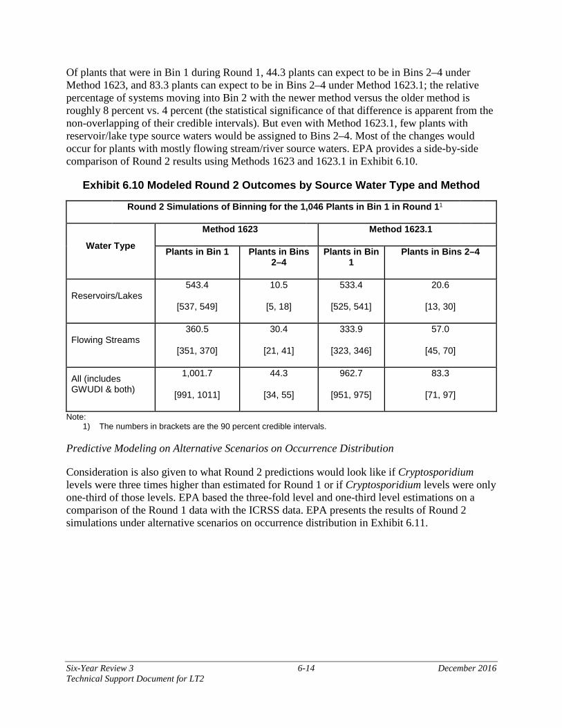
Six-Year Review 3 6-14 December 2016 Technical Support Document for LT2
Of plants that were in Bin 1 during Round 1, 44.3 plants can expect to be in Bins 2–4 under Method 1623, and 83.3 plants can expect to be in Bins 2–4 under Method 1623.1; the relative percentage of systems moving into Bin 2 with the newer method versus the older method is roughly 8 percent vs. 4 percent (the statistical significance of that difference is apparent from the non-overlapping of their credible intervals). But even with Method 1623.1, few plants with reservoir/lake type source waters would be assigned to Bins 2–4. Most of the changes would occur for plants with mostly flowing stream/river source waters. EPA provides a side-by-side comparison of Round 2 results using Methods 1623 and 1623.1 in Exhibit 6.10.
Exhibit 6.10 Modeled Round 2 Outcomes by Source Water Type and Method
Round 2 Simulations of Binning for the 1,046 Plants in Bin 1 in Round 11
Water Type
Method 1623 Method 1623.1
Plants in Bin 1 Plants in Bins 2–4
Plants in Bin 1
Plants in Bins 2–4
Reservoirs/Lakes 543.4
[537, 549]
10.5
[5, 18]
533.4
[525, 541]
20.6
[13, 30]
Flowing Streams 360.5
[351, 370]
30.4
[21, 41]
333.9
[323, 346]
57.0
[45, 70]
All (includes GWUDI & both)
1,001.7
[991, 1011]
44.3
[34, 55]
962.7
[951, 975]
83.3
[71, 97]
Note: 1) The numbers in brackets are the 90 percent credible intervals.
Predictive Modeling on Alternative Scenarios on Occurrence Distribution
Consideration is also given to what Round 2 predictions would look like if Cryptosporidium levels were three times higher than estimated for Round 1 or if Cryptosporidium levels were only one-third of those levels. EPA based the three-fold level and one-third level estimations on a comparison of the Round 1 data with the ICRSS data. EPA presents the results of Round 2 simulations under alternative scenarios on occurrence distribution in Exhibit 6.11.

Six-Year Review 3 6-15 December 2016 Technical Support Document for LT2
Exhibit 6.11 Plants in Bins 2–4 under Alternative Scenarios on Occurrence Distribution
Round 2 Simulations of Binning for the 1,046 Plants in Bin 1 in Round 1
Water Type Plants in Bin 1
in Round 1 % in Bins 2–4, Method
1623 % in Bins 2–4, Method
1623.1
×(3) ×(1) ×(1/3) ×(3) ×(1) ×(1/3) Reservoirs/Lakes 554 8.0% 1.9% 0.3% 12.9% 3.7% 0.6% Flowing Streams 391 24.2% 7.8% 1.3% 35.2% 14.6% 3.2% All (includes GWUDI & both)
1,046 14.3% 4.2% 0.7% 21.5% 8.0% 1.6%
If the underlying Cryptosporidium concentrations were three times higher during Round 2 than Round 1, use of either Method 1623 or Method 1623.1 would result in a greater proportion of plants falling into Bins 2–4. Under Method 1623, a 3-fold increase in Cryptosporidium concentration would roughly triple the number of plants in Bins 2–4. Under Method 1623.1, a 3-fold increase in Cryptosporidium count would more than double the number of plants in Bins 2–4, with roughly triple the number of reservoir/lake source water plants being placed in Bins 2–4 and roughly double the number of flowing stream source water plants being placed in Bins 2–4. However, Method 1623.1, with its greater baseline recovery rate, would still result in greater overall numbers of plants in Bins 2–4 than Method 1623.
If Cryptosporidium counts were reduced to one-third of the Round 1 levels, then use of either method would result in a decline in the number of plants in Bins 2–4. Under Method 1623, one-third of the concentration would yield less than one-fifth of the number of plants in Bins 2–4 (for both reservoir/lake source water plants and flowing stream source water plants). Under Method 1623.1, one-third of the concentration would also yield about one-fourth of the number of plants in Bins 2–4. Again, use of Method 1623.1 would still consistently place a greater proportion of plants in Bins 2–4 than Method 1623.
6.2 E. coli Indicator to Predict Cryptosporidium Occurrence
6.2.1 Background
As part of the review of the LT2, EPA reviewed the E. coli trigger level used to determine when small plants (serving fewer than 10,000 people) were required to monitor for Cryptosporidium.
The LT2 required large surface water systems serving 10,000 or more people to monitor for E. coli and Cryptosporidium in their source water monthly for two years to allow EPA to better evaluate the appropriateness of the trigger levels set in the LT2. Due to the high cost of Cryptosporidium monitoring, the LT2 allowed small systems to monitor for E. coli as an indicator for Cryptosporidium. These small systems could monitor E. coli on a twice- monthly basis for one year first. If the average E. coli concentration exceeded 10 colony-forming units (cfu) per 100 milliliters (mL) for reservoirs and lakes or 50 cfu/100 mL for flowing streams, as per the regulatory language, the system was required to monitor for Cryptosporidium. The LT2 staggered the monitoring schedules for four different size categories of systems. Systems serving at least 100,000 people began monitoring first, followed by systems serving 50,000 to 99,999

Six-Year Review 3 6-16 December 2016 Technical Support Document for LT2
people, followed by systems serving 10,000 to 49,999 people, followed by the small systems. The small systems began monitoring two years after the systems serving at least 100,000 began monitoring.
In 2010, EPA performed an analysis using data collected during the first year of Cryptosporidium and E. coli monitoring from systems serving 100,000 or more people. The intent of the 2010 analysis was to compare concentrations of Cryptosporidium and E. coli to determine the adequacy of the trigger level in the LT2. The analysis examined the paired Cryptosporidium and E. coli data from monitoring at WTPs in systems serving 100,000 or more people. EPA compared the trigger levels in the LT2 with a range of alternative trigger levels higher than those specified in the LT2 based on two criteria. The first criterion was the number of systems with Cryptosporidium levels with a concentration greater than or equal to 0.075 oocysts/L (these systems would require additional treatment). The second criterion was the number of small systems required to monitor for Cryptosporidium based on E. coli concentrations. This was estimated based on the occurrence and concentrations of E. coli from the large system monitoring, The 2010 analysis showed that increasing the E. coli trigger levels from the levels originally required by the LT2 (E. coli values of 10 and 50 cfu/100 mL for reservoirs/lakes and flowing streams, respectively) to 100 cfu/100 mL for both types of sources would result in a 50-percent decrease in the number of plants required to monitor for Cryptosporidium but only a 10-percent reduction in the number of plants using sources with high Cryptosporidium levels from being triggered into monitoring. Based on this analysis, EPA issued guidance to states allowing an alternative trigger level for small systems of 100 cfu/100 mL for both flowing streams and lakes or reservoirs. Some states, however, are prohibited from allowing the alternative trigger level by state law.
The purpose of the current analysis, which is described below, is to determine the adequacy of the 2010 alternative E. coli trigger level using the two years of available monitoring data for all large WTPs using Method 1623. The current analysis examines several other E. coli trigger levels for comparison.
6.2.2 Data Cleaning Process
Data EPA used in the analysis are from DCTS, with Cryptosporidium and E. coli data extracted separately (USEPA, 2016c). EPA cleaned the data to remove invalid, nonrepresentative or otherwise questionable data (the original data are also available at the same website). For example, EPA deleted data from inactive or seasonal water systems. Cryptosporidium and E. coli samples collected on the same date from the same plant were then paired and used to perform the analysis. More information on the data cleaning procedures used for EPA analysis is available on EPA’s website (USEPA, 2009b).
The first step in the data cleaning process was to calculate the E. coli concentrations of samples for which the lab entered raw data into the spreadsheet. For E. coli data, labs had a choice of entering the calculated concentration of E. coli or of entering the raw data from the analytical method. Calculations were conducted using the EPA-approved methods in the LT2 [40 CFR 141.704]. Additionally, EPA omitted a total of four samples from the analysis because the database contained insufficient data to calculate a concentration.

Six-Year Review 3 6-17 December 2016 Technical Support Document for LT2
After EPA calculated the E. coli concentrations, the Agency cleaned the data to remove data that could lead to erroneous or biased results. EPA used two separate data cleaning procedures and compared the results for each to see how they differed. The first data cleaning procedure exactly replicated the procedure used in the 2010 analysis to determine if the additional year of data changed the 2010 analysis in any way. Since the original 2010 analysis used in the guidance for the alternative trigger used only one year of monitoring data, some of the cleaning criteria were intended to ensure the validity of the additional data. With the data set now complete, some of the criteria were no longer applicable, so EPA conducted a second data cleaning procedure to assess the effect of changing these criteria. Therefore, the current analysis includes two sets of results, one for each data cleaning procedure used.
EPA removed data based on lab certification for Cryptosporidium, sample status and method reporting limits. Specifically, the following data were removed as part of the first data cleaning procedure.
• Samples analyzed by a laboratory that withdrew from EPA’s Cryptosporidium Laboratory Approval Program in September 2007.
• Any samples with a status code of “contested,” unless the sample collection date was the only issue contested.
• Any samples with a status code of “entered,” because this means that the samples had not been reviewed by the laboratory or the PWS for correctness.
• Any samples with a status code of “lab approved,” since these had not yet been reviewed by the PWS for correctness. These were removed unless the E. coli count was determined to be zero. EPA assumed if the result were zero, the PWS would not contest a sample. While it is possible allowing the zero results and not positive results might have introduced some bias, it allowed the greatest number of data points while not ignoring the possibility of error in the unreviewed samples.
• E. coli data for which the results were listed as “greater than” a number between 0 and 500. These data were considered to be uninformative.
• E. coli data for which the result was listed as “less than” a number greater than 10. The method detection limit on these samples was too high to provide meaningful results.
• Cryptosporidium matrix spike samples.
• Samples from systems listed as unfiltered or with no data in the plant filtration column. The E. coli trigger does not apply to unfiltered systems.
• Samples from PWSs that were inactive or seasonal (these systems would have had incomplete data and would require different methods for calculating averages).
For the second data cleaning procedure, fewer data were removed based on sample status. The only status-based results that were removed were those data that EPA contested or removed.

Six-Year Review 3 6-18 December 2016 Technical Support Document for LT2
EPA assumed that if the systems or laboratories desired to contest a sample, they had had sufficient time to do so. Also, since the laboratory that withdrew was approved up until the point it withdrew from the program, EPA kept its data. Data for small systems were also eliminated from the second data cleaning procedure because all small systems did not report data to DCTS and this could bias the results. Additionally, in the first data cleaning procedure, EPA categorized source water type based on the source water used in the first month of sampling. All Water Treatment Plants (WTPs), however, do not use the same source water type every month but may switch sources seasonally. Two hundred seventy-four plants were classified as either using both river and lake sources or switching sources during the sampling period. In the second data cleaning procedure, EPA categorized these plants by the source type they used more than 50 percent of the time. If no source type was used more than 50 percent of the time the plant was categorized as both.
In addition to removing these data, EPA performed several other steps to ready the data for analysis. These steps were completed for both data cleaning procedures:
• Units of measure were removed from the worksheet column used for the actual sample concentration value after confirming the correct units;
• Sample concentrations listed as “ND” were changed to a value of “0;”
• Sample concentrations listed as a number less than 10 were changed to a value of “0,” and;
• If the sample concentration was listed as a number greater than 500, the concentration was set to that number.
Setting nondetection results and results below the reporting limit to zero does not signify that there were no microbes in the sample but is rather a mathematical simplification for purposes of the analysis. While it may introduce some bias by skewing mean E. coli concentrations lower, EPA applied the change consistently throughout the analysis, and it is consistent with how data would be handled during sampling.
6.2.2.1 Data Pairing and Calculation
After EPA calculated the E. coli concentrations and cleaned the data, it paired E. coli and Cryptosporidium samples collected on the same day at the same WTP. If more than one sample was collected for a given microbiological analysis at a given plant on the same day, those values were averaged and the average value was considered the concentration on that day. EPA created two sets of paired data, one for each set of data cleaning criteria. The data cleaning and pairing operation resulted in 29,741 paired samples representing 1,356 plants using the original cleaning criteria. Of the 1,356 WTPs, 697 plants used reservoir/lake sources of supply, 618 plants used flowing streams and 41 plants used both types of supply. For the second set of cleaning criteria, there were 25,426 paired samples representing 1,372 WTPs. The number of paired samples per plant ranged from one to 105. Of the 1,372 WTPs, 702 plants used reservoir/lake supplies, 617 used flowing streams and 53 used both types of supply.

Six-Year Review 3 6-19 December 2016 Technical Support Document for LT2
6.2.3 Analysis
EPA used paired samples to calculate overall plant averages for E. coli and Cryptosporidium. Average counts were calculated according to methods required under the LT2. For E. coli, a straight average was calculated by summing the results of all samples collected for a given plant and dividing by the number of samples. For Cryptosporidium, the LT2 states that if 48 or more samples are taken, then a straight average can be used. If fewer than 48 samples are taken, the MRAA must be used. Therefore, a straight average was used to calculate plant averages for plants with 48 or more samples. For plants with fewer than 48 samples, calculation of the MRAAs was complicated by the fact that many plants did not have continuous data, either because of the data cleaning procedure or because of missed samples. Therefore, for plants with fewer than 12 samples, a simple average was used, as this would be equivalent to a RAA. For plants with 12 to 47 samples, EPA determined the first and last sample dates and calculated RAAs for each one year period beginning with the first sample. Each RAA was calculated using all samples collected in that one year period. The last RAA calculated was the one ending with the last sample. The highest of these RAAs, the MRAA, was selected as the plant average. This is consistent with the LT2 language, which requires systems to use the MRAA for treatment determination.
6.2.3.1 Criterion Values
Criteria used in this analysis are from Pope et al. (2002). Mathematically these criteria can be expressed by considering the true and false positives and negatives, as shown in Exhibit 6.12. Appendix B provides the detailed observed data for specific trigger values corresponding to the variables in Exhibit 5.12.
Exhibit 6.12 Definition of Variables Used in Analysis
Cryptosporidium concentration < 0.075 oocysts/L
Cryptosporidium concentration > 0.075 oocysts/L
E. coli concentration ≥ trigger value B D E. coli concentration < trigger value A C
Based on this definition of variables the eight criteria calculated can be defined as:
• False positives = B/(B+D);
• False negatives = C/(A+C);
• Sensitivity = D/(C+D);
• Specificity = A/(A+B);
• Plants Protectively Classified = (A+B+D)/(A+B+C+D);
• Plants Incorrectly Classified = C/(A+B+C+D);

Six-Year Review 3 6-20 December 2016 Technical Support Document for LT2
• Plants Correctly Exempted from Cryptosporidium Monitoring = A/(A+B+C+D), and;
• Plants Required to Monitor for Cryptosporidium = (B+D)/(A+B+C+D).
After EPA calculated the plant averages for E. coli and Cryptosporidium, EPA used the data to calculate values for the criteria above, for E. coli trigger levels of 10, 50, 75, 100, 150 and 200 cfu/100 mL. The formulas used to calculate each of these criterion values are provided in the bullets following Exhibit 6.12.
These criterion values were calculated for each of the two sets of data cleaning criteria. Exhibit 6.13 through Exhibit 6.15 show the calculated criterion values for each of the trigger levels examined for the original data cleaning criteria for each source water type.
Exhibit 6.16 through Exhibit 6.18 show the calculated criterion values for the revised cleaning criteria, again by source water type.
Exhibit 6.13 Criteria for Reservoirs and Lakes Using Original Cleaning Procedure
Levels of Testing Based on Various Trigger Levels E. coli Trigger Level (cfu/100 mL) Criterion 10 50 75 100 150 200 B/(B+D) (False Positives)
95.51% 92.91% 91.18% 90.28% 90.00% 84.62%
C/(A+C) (False Negatives) 1.56% 1.93% 1.85% 2.08% 2.44% 2.38%
D/(C+D) (Sensitivity) 70.00% 45.00% 45.00% 35.00% 20.00% 20.00%
A/(A+B) (Specificity) 55.98% 82.57% 86.26% 90.40% 94.68% 96.75%
(A+B+D)/(A+B+C+D) (Plants Protectively Classified)
99.14% 98.42% 98.42% 98.13% 97.70% 97.70%
C/(A+B+C+D) (Plants Incorrectly Classified 0.86% 1.58% 1.58% 1.87% 2.30% 2.30%
A/(A+B+C+D) (Plants Correctly Exempted from Cryptosporidium Monitoring)
54.38% 80.20% 83.79% 87.80% 91.97% 93.97%
(B+D)/(A+B+C+D) (Plants Required to Monitor for Cryptosporidium)
44.76% 18.22% 14.63% 10.33% 5.74% 3.73%

Six-Year Review 3 6-21 December 2016 Technical Support Document for LT2
Exhibit 6.14 Criteria for Rivers and Flowing Streams Using Original Cleaning Procedure
Levels of Testing Based on Various Trigger Levels E. coli Trigger Level (cfu/100 mL) Criterion 10 50 75 100 150 200 B/(B+D) (False Positives)
84.98% 81.13% 79.68% 77.15% 76.55% 72.97%
C/(A+C) (False Negatives) 1.52% 3.04% 3.90% 3.99% 5.61% 5.77%
D/(C+D) (Sensitivity) 97.33% 89.33% 84.00% 81.33% 70.67% 66.67% A/(A+B) (Specificity)
23.94% 46.96% 54.51% 62.06% 68.14% 75.14%
(A+B+D)/(A+B+C+D) (Plants Protectively Classified)
99.68% 98.71% 98.06% 97.73% 96.44% 95.95%
C/(A+B+C+D) (Plants Incorrectly Classified 0.32% 1.29% 1.94% 2.27% 3.56% 4.05%
A/(A+B+C+D) (Plants Correctly Exempted from Cryptosporidium Monitoring)
21.04% 41.26% 47.90% 54.53% 59.87% 66.02%
(B+D)/(A+B+C+D) (Plants Required to Monitor for Cryptosporidium)
78.64% 57.44% 50.16% 43.20% 36.57% 29.94%

Six-Year Review 3 6-22 December 2016 Technical Support Document for LT2
Exhibit 6.15 Criteria for All Samples Using Original Cleaning Procedure
Levels of Testing Based on Various Trigger Levels E. coli Trigger Level (cfu/100 mL) Criterion 10 50 75 100 150 200 B/(B+D) (False Positives)
88.92% 83.98% 82.23% 79.48% 78.31% 74.07%
C/(A+C) (False Negatives) 1.50% 2.32% 2.57% 2.77% 3.69% 3.77%
D/(C+D) (Sensitivity) 91.92% 79.80% 75.76% 71.72% 59.60% 56.57%
A/(A+B) (Specificity) 41.93% 67.06% 72.39% 78.12% 83.05% 87.27%
(A+B+D)/(A+B+C+D) (Plants Protectively Classified)
99.41% 98.53% 98.23% 97.94% 97.05% 96.83%
C/(A+B+C+D) (Plants Incorrectly Classified 0.59% 1.47% 1.77% 2.06% 2.95% 3.17%
A/(A+B+C+D) (Plants Correctly Exempted from Cryptosporidium Monitoring)
38.86% 62.17% 67.11% 72.42% 76.99% 80.90%
(B+D)/(A+B+C+D) (Plants Required to Monitor for Cryptosporidium)
60.55% 36.36% 31.12% 25.52% 20.06% 15.93%

Six-Year Review 3 6-23 December 2016 Technical Support Document for LT2
Exhibit 6.16 Criteria for Reservoirs and Lakes Using Revised Cleaning Procedure
Levels of Testing Based on Various Trigger Levels E. coli Trigger Level (cfu/100 mL) Criterion 10 50 75 100 150 200 B/(B+D) (False Positives)
94.72% 92.09% 90.20% 89.47% 90.00% 82.61%
C/(A+C) (False Negatives) 0.58% 1.78% 1.83% 2.08% 2.57% 2.50%
D/(C+D) (Sensitivity) 90.48% 52.38% 47.62% 38.10% 19.05% 19.05%
A/(A+B) (Specificity) 49.93% 81.20% 86.49% 90.01% 94.71% 97.21%
(A+B+D)/(A+B+C+D) (Plants Protectively Classified)
99.72% 98.58% 98.43% 98.15% 97.58% 97.58%
C/(A+B+C+D) (Plants Incorrectly Classified 0.28% 1.42% 1.57% 1.85% 2.42% 2.42%
A/(A+B+C+D) (Plants Correctly Exempted from Cryptosporidium Monitoring)
48.43% 78.77% 83.90% 87.32% 91.88% 94.30%
(B+D)/(A+B+C+D) (Plants Required to Monitor for Cryptosporidium)
51.28% 19.80% 14.53% 10.83% 5.70% 3.28%

Six-Year Review 3 6-24 December 2016 Technical Support Document for LT2
Exhibit 6.17 Criteria for Rivers and Streams Using Revised Cleaning Procedure
Levels of Testing Based on Various Trigger Levels E. coli Trigger Level (cfu/100 mL) Criterion 10 50 75 100 150 200 B/(B+D) (False Positives)
87.53% 84.06% 82.84% 81.03% 80.86% 77.78%
C/(A+C) (False Negatives) 0.83% 2.94% 3.50% 4.12% 5.64% 5.61%
D/(C+D) (Sensitivity) 98.41% 87.30% 82.54% 76.19% 63.49% 60.32%
A/(A+B) (Specificity) 21.48% 47.65% 54.69% 63.00% 69.49% 75.99%
(A+B+D)/(A+B+C+D) (Plants Protectively Classified)
99.84% 98.70% 98.22% 97.57% 96.27% 95.95%
C/(A+B+C+D) (Plants Incorrectly Classified 0.16% 1.30% 1.78% 2.43% 3.73% 4.05%
A/(A+B+C+D) (Plants Correctly Exempted from Cryptosporidium Monitoring)
19.29% 42.79% 49.11% 56.56% 62.40% 68.23%
(B+D)/(A+B+C+D) (Plants Required to Monitor for Cryptosporidium)
80.55% 55.92% 49.11% 41.00% 33.87% 27.71%

Six-Year Review 3 6-25 December 2016 Technical Support Document for LT2
Exhibit 6.18 Criteria for All Samples Using Revised Cleaning Procedure
Levels of Testing Based on Various Trigger Levels E. coli Trigger Level (cfu/100 mL) Criterion 10 50 75 100 150 200 B/(B+D) (False Positives)
90.36% 86.17% 84.38% 82.54% 81.78% 78.00%
C/(A+C) (False Negatives) 0.83% 2.41% 2.62% 3.00% 3.86% 3.92%
D/(C+D) (Sensitivity) 95.56% 76.67% 72.22% 65.56% 52.22% 48.89%
A/(A+B) (Specificity) 37.13% 66.46% 72.62% 78.24% 83.54% 87.83%
(A+B+D)/(A+B+C+D) (Plants Protectively Classified)
99.71% 98.47% 98.18% 97.74% 96.87% 96.65%
C/(A+B+C+D) (Plants Incorrectly Classified 0.29% 1.53% 1.82% 2.26% 3.13% 3.35%
A/(A+B+C+D) (Plants Correctly Exempted from Cryptosporidium Monitoring)
34.69% 62.10% 67.86% 73.10% 78.06% 82.07%
(B+D)/(A+B+C+D) (Plants Required to Monitor for Cryptosporidium)
65.01% 36.37% 30.32% 24.64% 18.80% 14.58%
As expected, E. coli and Cryptosporidium values are higher in flowing streams than they are in reservoirs and lakes. The qualitative trends, however, are similar for both source types. For both source types specificity (the proportion of Cryptosporidium negatives that are correctly identified by E. coli negatives) increases with higher trigger levels, while sensitivity (the proportion of Cryptosporidium positives that are correctly identified by E. coli positives) decreases. Selecting the proper trigger level involves balancing the number of plants with high Cryptosporidium concentrations properly triggered into monitoring versus those with low Cryptosporidium concentrations correctly allowed to avoid monitoring.
There does not seem to be any significant difference between criteria calculated based on the original cleaning procedure (Exhibit 6.13 through Exhibit 6.15) and criteria calculated based on the revised cleaning procedure (Exhibit 6.16 through Exhibit 6.18), and the two procedures lead to similar trends and conclusions. There are slight differences in the criterion values, but they do not seem to point to any clear bias. The revised cleaning procedure shows slightly higher false positives and false negatives with a lower specificity than the original cleaning procedure. The differences appear to be mostly in the river and stream category. There are two possible causes for any bias. The first is the exclusion of the Schedule 4 systems in the revised cleaning procedure. Schedule 4 systems were most likely triggered into Cryptosporidium monitoring by high E. coli concentrations, so they tend to have higher E. coli and Cryptosporidium concentrations. This could account for the slightly lower specificity in the revised cleaning

Six-Year Review 3 6-26 December 2016 Technical Support Document for LT2
procedure criterion values, as some of the higher E. coli and Cryptosporidium samples were eliminated, leading to less specificity. The other possible cause of bias may be the inclusion of the laboratory and of previously unreviewed data in the revised cleaning procedure data. If these data were skewed, that might also account for some difference.
In general, the sensitivity is very high at the lower E. coli trigger levels. This means that at the lower trigger levels, most plants that have sources of supply with Cryptosporidium concentrations greater than the binning level (i.e., Bin 1 requires a Cryptosporidium concentration < 0.075 oocysts per liter) would have been triggered into monitoring based on their E. coli data. This trend is not as pronounced in reservoirs and lakes as it is in flowing streams. The number of plants required to monitor and the number of plants incorrectly classified, however, are also higher at the lower trigger values. As the trigger level is increased, the specificity drops, and the number of plants correctly exempted from monitoring increases.
6.2.4 Results and Discussion
The effectiveness of the alternative E. coli trigger can be thought of using two criteria.
1. Sensitivity. Plants that have high Cryptosporidium concentrations (>0.075 oocysts/L) would be correctly triggered into monitoring based on their E. coli monitoring.
2. The total number of plants triggered into Cryptosporidium monitoring. Ideally, only those plants with high Cryptosporidium would be triggered into monitoring.
The most effective trigger level is that which minimizes the plants required to unnecessarily monitor while maximizing the number of plants with high Cryptosporidium that are triggered into monitoring.
6.2.4.1 Plants Monitoring Versus Plants Triggered Into Treatment
Using the calculated criterion values for each E. coli trigger level and scaling up by the total number of small WTPs for each source water type, EPA completed the following estimates.
• The total number of small plants that would be required to monitor based on E. coli results.
• The total number of small plants with Cryptosporidium greater than or equal to 0.075 oocysts/L that would be correctly assigned to treatment bins.
EPA determined the total number of small plants of each source water type by assuming that small systems have the same percentage of different source water types as the systems in DCTS and multiplying by the total number of small surface water systems from EPA’s State Drinking Water Information System database. This analysis assumes that the underlying Cryptosporidium and E. coli concentrations are the same for large and small systems. EPA multiplied the percentage of plants required to monitor for each source water type by the total number of small systems for that source water type to obtain the total number of small plants that would be required to monitor for Cryptosporidium. Likewise, the percentage of small plants with greater than or equal to 0.075 oocysts/L for each source water type was multiplied by the total number of
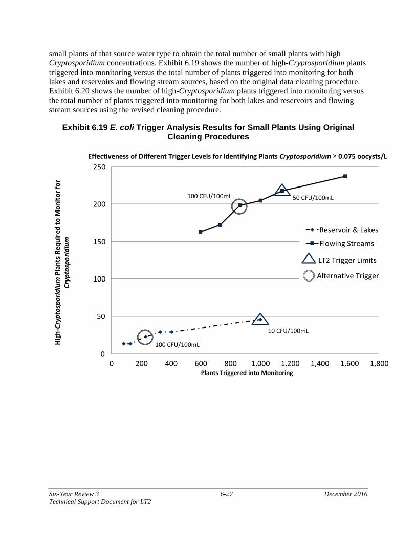
Six-Year Review 3 6-27 December 2016 Technical Support Document for LT2
small plants of that source water type to obtain the total number of small plants with high Cryptosporidium concentrations. Exhibit 6.19 shows the number of high-Cryptosporidium plants triggered into monitoring versus the total number of plants triggered into monitoring for both lakes and reservoirs and flowing stream sources, based on the original data cleaning procedure. Exhibit 6.20 shows the number of high-Cryptosporidium plants triggered into monitoring versus the total number of plants triggered into monitoring for both lakes and reservoirs and flowing stream sources using the revised cleaning procedure.
Exhibit 6.19 E. coli Trigger Analysis Results for Small Plants Using Original Cleaning Procedures
0
50
100
150
200
250
0 200 400 600 800 1,000 1,200 1,400 1,600 1,800 Plants Triggered into Monitoring
Effectiveness of Different Trigger Levels for Identifying Plants Cryptosporidium ≥ 0.075 oocysts/L
Reservoir & Lakes Flowing Streams
Alternative Trigger
LT2 Trigger Limits
50 CFU/100mL 100 CFU/100mL
10 CFU/100mL
100 CFU/100mL High
-Cry
ptos
porid
ium
Pla
nts R
equi
red
to M
onito
r for
Cr
ypto
spor
idiu
m

Six-Year Review 3 6-28 December 2016 Technical Support Document for LT2
Exhibit 6.20 E. coli Trigger Analysis Results for Small Plants Using Revised Cleaning Procedures
High
-Cry
ptos
porid
ium
Pla
nts
Requ
ired
to M
onito
r for
Cry
ptos
porid
ium
Effectiveness of E. coli Monitoring for Identifying High-Cryptosporidium Plants

Six-Year Review 3 6-29 December 2016 Technical Support Document for LT2
As the trigger level drops, an increased number of plants with high Cryptosporidium required to monitor increases. While each lower trigger level has a larger number of high Cryptosporidium plants triggered, the increase is greatest between the 150 and 100 cfu/100 mL trigger values for both the original and revised data cleaning procedures. The revised cleaning procedures described in Section 6.2.2 resulted in 26 plants being triggered into Cryptosporidium monitoring at the alternative trigger level for lakes and reservoirs, compared to 23 plants with the original cleaning procedures. For flowing streams the opposite trend was observed with the revised cleaning procedures resulting in 156 plants triggered and the original cleaning procedures resulting in 198 plants triggered.
6.2.4.2 Analysis of Current Trigger Level and Comparison to Previous Data
Exhibit 6.21 shows the same graph that was prepared for the original alternative trigger analysis in 2010.
Exhibit 6.21 2010 Trigger Analysis Results
Effectiveness of Monitoring to Capture High-Cryptosporidium Plants
Hig
h-Cr
ypto
spor
idiu
m P
lant
s Req
uire
d to
Mon
itor f
or C
rypt
ospo
ridiu
m
Plants Required to Monitor for Cryptosporidium
Qualitatively the graphs are very similar to the graphs from the current analysis. They are both flatter toward the right hand side of the graph and show an inflection point near the alternative trigger level of 100 cfu/100 mL.
6.2.4.3 Recommended Trigger Level
As both the original 2010 graphs and those completed for this analysis show inflection points at a trigger level of 100 cfu/100 mL, the alternative trigger level is supported by the data collected

Six-Year Review 3 6-30 December 2016 Technical Support Document for LT2
during the first round of Cryptosporidium monitoring. Exhibit 6.22 shows the reductions in each of the criteria between the LT2 trigger level and a trigger level of 75, 100 or 150 cfu/100 mL.
Exhibit 6.22 Percent Reduction in Plants Required to Monitor with Alternate Trigger Levels
Reduction in Plants Required to Monitor from Rule Trigger
Levels1 to Alternate Trigger Levels2 Criterion Alternate Trigger 75 100 150
Original Cleaning Procedure
High-Cryptosporidium Plants Triggered
Reservoirs/Lakes 36% 50% 71% Flowing Streams 6% 9% 21%
Plants Required to Monitor
Reservoirs/Lakes 67% 77% 87% Flowing Streams 13% 25% 36%
Revised Cleaning Procedure
High-Cryptosporidium Plants Triggered
Reservoirs/Lakes 47% 58% 79% Flowing Streams 5% 13% 27%
Plants Required to Monitor
Reservoirs/Lakes 72% 79% 89% Flowing Streams 12% 27% 39%
Notes: 1) 10 cfu/100 mL for reservoirs/lakes and 50 cfu/100 mL for flowing streams. 2) 75, 100 or 150 cfu/100 mL for all types of supply sources.
Comparing the original LT2 trigger values to the alternative trigger value of 100 cfu/100 mL reveals a reduction in plants required to monitor by 77 percent for reservoirs/lakes and 25 percent for flowing streams based on the original cleaning procedures. The reduction is 79 percent for reservoirs and lakes and 27 percent for flowing streams based on the revised cleaning procedures. This results in a 50-percent reduction in high-Cryptosporidium plants being triggered for reservoirs and lakes and 9 percent for flowing streams for the original cleaning procedures and a 58-percent reduction for reservoirs and lakes and a 13-percent difference for rivers and streams based on the revised data cleaning procedures.
Using the original cleaning procedure, a trigger value of 150 cfu/100 mL would result in a 71-percent drop in high Cryptosporidium plants being triggered for lakes and reservoirs and 21 percent for flowing streams while reducing the number of plants monitoring by 87 and 36 percent, respectively. Using the revised cleaning procedure a trigger value of 150 cfu/100 mL would result in a 79-percent drop in high Cryptosporidium plants triggered for reservoirs and lakes and 27-percent reduction for rivers and streams, while reducing the number of plants monitoring by 89 and 39 percent, respectively.
The inflection point at the alternative trigger value of 100 cfu/100 mL indicates this is where the incremental number of high-Cryptosporidium plants correctly triggered is maximized versus minimizing the number of small plants required to perform Cryptosporidium monitoring. Moreover, use of the 100 cfu/100 mL alternative indicator allows for a large reduction in plants required to monitor for Cryptosporidium, with only a small reduction in plants with high Cryptosporidium not being required to monitor.

Six-Year Review 3 6-31 December 2016 Technical Support Document for LT2
6.3 Cooccurrence of Cryptosporidium and Other Pathogens of Concern
6.3.1 Giardia and Cryptosporidium Cooccurrence from ICR Supplemental Survey Data
6.3.1.1 Background on the ICR Supplemental Survey
The ICRSS required Method 1623 for measurement of Cryptosporidium and Giardia in the surface water sources of 87 drinking water systems. Forty of the systems were medium sized (serving between 10,000 and 100,000 people) and 47 were large (serving at least 100,000 people). Each system’s source water was categorized as one of three types (flowing streams, reservoirs/lakes or both). The distribution of sources by size and water type is shown in Exhibit 6.23.
Exhibit 6.23 Distribution of ICRSS Source Waters by System Size and Water Type
Water Type System Size Medium Large Flowing Stream (Type 1) 17 16 Lake/Reservoir (Type 2) 19 29 Both Flowing Stream and Lake/Reservoir (Type 3)
4 2
Total = 40 Total = 47
6.3.1.2 Summary of ICRSS Data
Over a 12-month period, beginning in March 1999, participating systems sampled each source twice per month for Cryptosporidium, although some systems assayed extra samples while others had missing samples. Testing for Giardia began in July 1999; samples taken earlier were assayed only for Cryptosporidium. A total of 2,086 samples were assayed (average of 24 samples per source) for Cryptosporidium and 1,350 of these samples were also assayed for Giardia (average of 15.5 per source). Exhibit 6.24 provides some additional summary statistics.
Exhibit 6.24 ICRSS Summary Statistics for Cryptosporidium and Giardia
Statistic Cryptosporidium Summary Value
Giardia Summary Value
Average Volume Assayed 10.11 L 10.17 L Total Oocysts Counted 1057 3255 Average Concentration (total count / total volume)
0.050/L 0.237/L
Percent of Samples with No Detections
86.4% 67.1%
Percent of Sources with No Detections
20.7% 18.4%
Exhibit 6.25 is a scatterplot showing the observed mean concentrations for the 87 sources. A small constant (0.005) was added so sources with no detections could be displayed. Some points overlap others. In particular, the point in the lower left represents all of the sources having no

Six-Year Review 3 6-32 December 2016 Technical Support Document for LT2
detections for either Cryptosporidium or Giardia. Exhibit 6.25 suggests a positive correlation between Cryptosporidium and Giardia and shows greater overall occurrence for flowing streams than for lakes and reservoirs.
Exhibit 6.25 Scatterplot of Observed Mean Concentrations for 87 Source Waters
6.3.1.3 Statistical Modeling
EPA employed a simple model to describe the co-occurrence of Cryptosporidium and Giardia. For each source water, EPA assumed recoverable protozoa of the two types are independently lognormally distributed over time. The number counted in a sample volume of V liters assayed is assumed to be a Poisson random variable with parameter V * C, where C is the unobserved concentration of recoverable oocysts in the waterbody at the time of sampling. Between source waters, EPA assumed the mean concentrations of Cryptosporidium and Giardia to be lognormally distributed with a variance-covariance structure. This simple model therefore includes random effects for source waters, but no effects for water type or for system size. The model includes a correlation coefficient to reveal the degree to which levels of the two protozoa are correlated across sources. EPA also evaluated two more complex models. The first of these includes effects for water type (two additional parameters), but not for system size, while the second includes an effect for each combination of water type and system size (five additional parameters).

Six-Year Review 3 6-33 December 2016 Technical Support Document for LT2
EPA estimated parameters using Bayesian MCMC methods. Deviance information criterion (DIC), a measure of model quality, is monitored for each model. Higher DIC values indicate decreasing model quality. Accordingly, the results, shown in Exhibit 6.26, reveal the more complex models (Model 2 and Model 3) perform better than the simple model (Model 1), which had no effects for water type or system size. Moreover, Model 2 has the lowest DIC and is judged to be the best of the three models, though the DIC for Model 3 is close to Model 2.
Exhibit 6.26 Deviance Information Criterion Model Results
Model Name Features DIC Model 1 Effects for Sources 4662.5 Model 2 Model 1 + Effects for
Water Types 4648.3
Model 3 Model 2 + Effects for System Size
4649.7
The following summarizes the estimates (posterior means) for several high-level parameters.
• The effect of Type 2 (Lake/Reservoir) water on Cryptosporidium is -1.716.
o Reservoirs and lakes have significantly less Cryptosporidium than flowing streams.
o Overall, the levels in reservoirs and lakes are lower by about a factor of 5.5 (exp(1.716)).
• The effect of Type 3 (both flowing stream and lake/reservoir) water on Cryptosporidium is -1.496.
o Sources of type “both” have significantly less Cryptosporidium than flowing streams.
o Overall levels in sources of type “both” are lower by about a factor of 4.5 (exp(1.496)).
o Levels in reservoirs and lakes are not significantly different from levels in category “both.”
• The effect of Type 2 (lake/reservoir) water on Giardia is -2.938.
o Reservoirs and lakes have significantly less Giardia than flowing streams.
o Overall, the levels in reservoirs and lakes are lower by about a factor of 19 (exp(2.938)).
• The effect of Type 3 (both flowing stream and lake/reservoir) water on Giardia is -2.516.
o Sources of type “both” have significantly less Giardia than flowing streams.

Six-Year Review 3 6-34 December 2016 Technical Support Document for LT2
o Overall levels in sources of type “both” are lower by about a factor of 12 (exp(2.516)).
o Levels in reservoirs and lakes are not significantly different from levels in category “both.”
• The correlation coefficient is 0.637.
o Significantly greater than zero (positive correlation between average levels of Cryptosporidium and Giardia).
o Giardia levels explain nearly two-thirds of the between-source variance of Cryptosporidium. Likewise, Cryptosporidium levels explain nearly two-thirds of the between-source variance of Giardia levels.
• Within-location standard deviation of ln(Cryptosporidium concentration) is 2.001.
o For an individual source water, the ratio of the 97.5th percentile concentration to 2.5th percentile concentration is about 2600.
• Within-location standard deviation of ln(Giardia concentration) is 1.396.
o For an individual source water, the ratio of the 97.5th percentile concentration to 2.5th percentile concentration is about 240.
o Giardia has lower within-source variability (on a log scale) than does Cryptosporidium.
6.3.1.4 Results
The positive correlation of Cryptosporidium and Giardia indicates that locations with high Cryptosporidium occurrence tend also to have high Giardia levels. Moreover, by reducing Cryptosporidium exposures, plants whose Round 1 Cryptosporidium data place them in Bins 2-4 may also be reducing higher-than-average Giardia exposures. Median model parameter estimate calculations based on the model; using those estimates led to the following findings.
• Occurrences of both Giardia and Cryptosporidium are greater in flowing streams than in reservoirs and lakes.
o On average, flowing streams have nearly 20 times as much Giardia as do reservoirs and lakes.
o On average, flowing streams have nearly six times as much Cryptosporidium as do reservoirs and lakes.
• Across sources of either type, Cryptosporidium and Giardia are positively correlated, signifying that sources with high Cryptosporidium occurrence tend to also have high Giardia occurrence.

Six-Year Review 3 6-35 December 2016 Technical Support Document for LT2
o Of all Cryptosporidium in flowing streams, more than 80 percent occur in streams with mean concentrations greater than 0.075 oocysts/L. Most flowing streams (approximately 60 percent of them) have mean concentrations less than 0.075 oocysts/L.
o Nearly 80 percent of the Giardia in flowing streams occur in the 40 percent of locations where mean Cryptosporidium concentrations exceed 0.075 oocysts/L.
o Of all Cryptosporidium in reservoirs and lakes, about 30 percent occur in those with mean concentrations greater than 0.075 oocysts/L, but only about 2 percent of reservoirs and lakes have mean concentrations greater than 0.075 oocysts/L.
o About 25 percent of the Giardia in reservoirs and lakes occur in the 2 percent of reservoirs and lakes where mean Cryptosporidium concentrations exceed 0.075 oocysts/L.
• In both water types, average Giardia occurrence exceeds that of Cryptosporidium.
o In flowing streams, the average Giardia concentration is about nine times the average Cryptosporidium concentration.
o In reservoirs and lakes, the average Giardia concentration is about three times the average Cryptosporidium concentration.
EPA based these findings on median parameter values and did not consider parameter uncertainty. The ratios and percentages stated are best estimates, based on the ICRSS data. Data from Round 1 monitoring reveal that Cryptosporidium occurrence levels are significantly lower than they were at the time of the ICRSS. Without assays for both Cryptosporidium and Giardia, however, the Round 1 data are not useful for testing the model described above. Levels of Giardia may have changed, due to the same unknown factors that led to the reduction in Cryptosporidium. Also, the strength of the correlation may have changed, but new data would be needed to inform EPA’s understanding of the correlation.
6.4 Summary
In developing the LT2, EPA relied on data from surveys conducted in earlier years (1997-1998 for the ICR survey and 1999-2000 for the ICRSS). Statistical modeling of those data revealed differing occurrence levels due to true differences in occurrence, systematic differences in the measurement methods or other factors. Recognizing that the LT2 would not be implemented for some time, EPA considered the differences as evidence that occurrence levels could vary from year-to-year. Costs and benefits were derived under these alternative models of occurrence to represent uncertainty about future occurrence.
In the LT2 EA (USEPA, 2005a), EPA based estimated benefits only on reduced exposure to Cryptosporidium, although treatment and other actions designed to reduce Cryptosporidium exposures were also assumed to reduce exposures to other pathogens. A more recent analysis of ICRSS data identified a strong correlation between average levels of Cryptosporidium and Giardia. This suggests that the LT2 controls aimed primarily at Cryptosporidium removal may

Six-Year Review 3 6-36 December 2016 Technical Support Document for LT2
be effective at lowering exposures to Giardia as well. The benefit of these additional reductions in Giardia in finished water is believed to be supplemental to existing treatment, however, due to the effectiveness of chlorine and other disinfectants used for Giardia inactivation.
The Round 1 monitoring data reveal that Cryptosporidium occurrence levels are significantly lower than predicted by any of the earlier, survey-based models. The numbers of plants falling into action bins (Bins 2, 3 and 4) was smaller than expected, so both the costs and benefits related to binning and treatment are lower than predicted in the LT2 EA. It is not clear, however, whether the low occurrence in Round 1 is due to random year-to-year differences or part of a systematic decline that can be expected to continue through Round 2 monitoring. The rationale for Round 2 remains valid: to determine where source water occurrence has changed to the extent that changes in treatment are needed.
EPA also used the Round 1 monitoring data to better understand the utility of E. coli as a trigger for Cryptosporidium monitoring by small systems. The complete Round 1 dataset supports the alternative trigger levels that were based on data available in 2010. Compared to the original LT2 trigger levels (10 cfu/100 mL for reservoirs/lakes and 50 cfu/100 mL for flowing streams), the alternative trigger (100 cfu/100 mL for all source waters) greatly reduces the number of plants required to monitor for Cryptosporidium, with only a small reduction of monitoring among plants with high levels of Cryptosporidium.
Finally, EPA used statistical models based on the Round 1 data to gauge the sensitivity of Round 2 predictions to systematic changes in recovery (due to using Method 1623.1 rather than 1622/1623) and occurrence. As expected, the number of plants requiring additional treatment increases with systematic increases in occurrence and recovery and decreases with systematic decreases in occurrence and recovery.

Six-Year Review 3 7-1 December 2016 Technical Support Document for LT2
7 LT2 Microbial Toolbox and Other Tools
Public water systems (PWSs) required to provide additional Cryptosporidium treatment under the Long Term 2 Enhanced Surface Water Treatment Rule (LT2) can select from a variety of microbial toolbox treatment and management strategy options. The LT2 Toolbox Guidance Manual (USEPA, 2010c) provides technical information on applying the toolbox options. This section serves to analyze information on the use and effectiveness of risk mitigation tools in the toolbox. This chapter focuses on the relevant new information published since 2006, but includes some older papers as needed for context.
Where information is available this section identifies and describes the types of challenges encountered and how they were overcome by water systems and state programs when implementing the microbial toolbox requirements of the LT2. The implementation issues described are based on input from various EPA offices and regions, along with the review of several related documents (e.g., utility reports, journal publications). This document also provides additional input received from stakeholders during public stakeholder meetings held by EPA.
EPA’s literature review efforts focused on obtaining case studies of water systems placed in Bins 2, 3 and 4 illustrating challenges with implementation and approaches to their resolution. Additional information EPA reviewed identifies, in some cases, which toolbox components systems are implementing. EPA also contacted nine utilities assigned to either Bins 2 or 3 regarding the use of the microbial toolbox tools or other tools. The contacted utilities all must provide additional treatment under the LT2. Appendix C summarizes the information gathered.
Background on the LT2 Microbial Toolbox Requirements
The LT2 microbial toolbox provides technical information on applying the “toolbox” of Cryptosporidium treatment and management strategies that are part of the Long Term 2 Enhanced Surface Water Treatment Rule. This toolbox, referred to in the LT2 as the microbial toolbox, covers the following categories: source protection, pre-filtration, treatment performance, additional filtration and inactivation options. The microbial and disinfection byproducts (MDBP) federal advisory committee (FAC) recommended the toolbox options as part of a multiple barrier treatment process that provides a number of protective “layers” against drinking water contamination. These options emphasize using more than one method to minimize, remove or inactivate microorganisms and minimize disinfection byproducts (DBPs).
Under the LT2, systems receive prescribed treatment credits by meeting conditions for one toolbox option or a combination of options. States are responsible for establishing performance criteria for many of the options and for developing monitoring and reporting requirements to determine compliance with the established criteria. Technical guidance documents and implementation guidance are available to assist with understanding the toolbox options, site-specific validation or demonstrated performance considerations, and compliance monitoring recommendations (USEPA, 2006c; 2007; 2010c).
Background on the LT2 Microbial Toolbox Implementation Issues

Six-Year Review 3 7-2 December 2016 Technical Support Document for LT2
The compliance dates for implementing toolbox options resulting from Round 1 monitoring range from April 2012 for systems on Schedule 1 to October 2014 for systems on Schedule 4. If additional time is necessary for capital improvements, the compliance date may be extended (if approved by the state) by up to two years [40 CFR 141.713(c)]. In addition, systems on Schedule 4 that are conducting Escherichia coli sampling prior to any Cryptosporidium sampling may have their compliance schedule extended to October 2016. Systems should have already completed their Round 1 source water sampling, determined if they are required to install treatment, and selected their toolbox options. However, installation or implementation of the options may still be in progress in some cases. Therefore, the following is a preliminary summary of implementation issues reported to EPA regarding the microbial toolbox options.
During the November 15, 2012 meeting held by EPA the microbial toolbox was discussed, along with two states’ perspectives on toolbox options, and results from a water industry survey (Cornwell et al., 2012). Input from state and water utility representatives included:
• Some tools are too complex for systems to implement and states to review;
• Some tools have capital cost or site issues that limit their use;
• In some cases, states cannot use guidance documents for compliance purposes. The Ultraviolet Disinfection Guidance Manual (UVDGM), in particular, may be too complicated and difficult to use, and;
• States may also benefit from access to a designated expert who can provide technical assistance for each technology or tool.
The degree to which implementation issues have been identified varies by the option in the microbial toolbox. Systems vary widely in their use of the different tools available in the microbial toolbox. This document discusses each of the microbial toolbox options in order of their appearance in the LT2. The discussion of the toolbox options is followed by a discussion of ceramic membranes and other potential tools that are not part of the microbial toolbox.
7.1 Summary of Data on Toolbox Options and Treatment Credits
Exhibit 7.1 provides a summary of the toolbox options and the review findings. For each toolbox option, the table indicates whether the literature reviewed provided new information on risk reduction from Cryptosporidium, risk reduction from other pathogens of concern, and design and implementation criteria. For each “yes” entry in this table, there is a summary of the literature reviewed in the following subsections.

Six-Year Review 3 7-3 December 2016 Technical Support Document for LT2
Exhibit 7.1 Summary of New Information on the LT2 Microbial Toolbox Options
Is There New Information Related to:
Microbial Toolbox Option Risk Reduction from
Cryptosporidium?
Risk Reduction from Other
Pathogens of Concern?
Design and Implementation
Criteria?
Watershed Control Program (WCP)
Yes See Section 7.3.1
Yes See Section 7.3.1
No
Alternative Source / Intake Management
Yes See Section 7.3.2
Yes See Section 7.3.2 No
Presedimentation Basin with Coagulation No No No
Two-stage Lime Softening No No No Bank Filtration (BF) Yes
See Section 7.3.5 Yes
See Section 7.3.5 Yes
See Section 7.3.5 Combined Filter Performance No No No Individual Filter Performance No No No Demonstration of Performance (DOP)
Yes See Section 7.3.8 No Yes
See Section 7.3.8 Bag or Cartridge Filters (individual filters)1
Yes See Section 7.3.9
Yes See Section 7.3.9
Yes See Section 7.3.9
Bag or Cartridge Filters (in series) 1
Yes See Section 7.3.9
Yes See Section 7.3.9
Yes See Section 7.3.9
Membrane Filtration Yes See Section 7.3.10
Yes See Section 7.3.10
Yes See Section 7.3.10
Second Stage Filtration Yes See Section 7.3.11
Yes See Section 7.3.11
Yes See Section 7.3.11
Slow Sand Filters Yes See Section 7.3.12
Yes See Section 7.3.12
Yes See Section 7.3.12
Chlorine Dioxide No
Yes See Section 7.3.13
Yes See Section 7.3.13
Ozone Yes See Section 7.3.14
Yes See Section 7.3.14
Yes See Section 7.3.14
Ultraviolet (UV) Disinfection Yes See Section 7.3.15
Yes See Section 7.3.15
Yes See Section 7.3.15
Note: 1) EPA did not identify articles specific to bag or cartridge filters within a treatment plant as a post-treatment
process for obtaining additional removal credit under the LT2. The treatment units discussed in the literature review were composite, point-of-use units, and are described in Section 7.3.9.

Six-Year Review 3 7-4 December 2016 Technical Support Document for LT2
Exhibit 7.2 provides a summary of each of the LT2 microbial toolbox options and compares the public health protection for Cryptosporidium relative to the protection each tool provides for other organisms. For bacteria and viruses the data presented are for those species of potential drinking water concern that are known to be the most resistant to the disinfectants. This comparison can help provide regulators and the public with insight into the secondary benefits of application of the LT2 toolbox tools beyond Cryptosporidium reduction. For several of the toolbox options, the literature reviewed did not provide information to assess the relative protection provided for other organisms compared to Cryptosporidium. This chapter provides a discussion of the relative protection of each of the tools in the relevant section, where available.
Exhibit 7.2 Comparative Effectiveness of Tools for Different Organisms
Toolbox Option
Cryptosporidium (credit for
toolbox option) Organism size 4 to 6 microns1
Giardia Organism size
7 to 14 microns1
Bacteria Organism size
0.2 to 5 microns2
Viruses Organism size
0.005 to 0.1 microns2
Source Toolbox Components WCP 0.5-log No information found indicating relative protection by
organism type.
Alternative Source/ Intake Management
Not prescribed No information found indicating relative protection by organism type.
Prefiltration Toolbox Components Presedimentation Basin w/Coagulation
0.5-log No information found indicating relative protection by organism type.
Two-stage Lime Softening
0.5-log No information found indicating relative protection by organism type.
BF 0.5 to 1-log No information found indicating relative protection by organism type.
Treatment Performance Toolbox Components Combined Filter Performance
0.5-log No information found indicating relative protection by organism type.
Individual Filter Performance
0.5-log No information found indicating relative protection by organism type.
DOP State decision Relative protection cannot be determined as demonstration could be for a wide variety of treatment
technologies.
Additional Filtration Toolbox Options Bag or Cartridge Filters—individual (Pore size down to 0.2 µm for cartridge and 1 µm for bag3)
≤2-log Similar effectiveness as Cryptosporidium
based on pore size.
Less effective than for
Cryptosporidium. 1
Less effective than for
Cryptosporidium. Not reliably
capable of 4-log virus removal.1
Bag or Cartridge Filters—series
≤2.5-log Similar to effectiveness for Cryptosporidium
based on pore size.
Less effective than for
Cryptosporidium.1
Less effective than for
Cryptosporidium. Not reliably
capable of 4-log virus removal.1

Six-Year Review 3 7-5 December 2016 Technical Support Document for LT2
Toolbox Option
Cryptosporidium (credit for
toolbox option) Organism size 4 to 6 microns1
Giardia Organism size
7 to 14 microns1
Bacteria Organism size
0.2 to 5 microns2
Viruses Organism size
0.005 to 0.1 microns2
Membrane Filtration—Reverse Osmosis (Nominal pore size 0.0001 µm1)
Log removal credit based on
demonstration (Capable of ≥2-log Cryptosporidium
removal1)
Capable of ≥3-log Giardia removal.1
Capable of removal of
bacteria, but not absolute.1
Capable of ≥4-log virus removal.1
Membrane Filtration—Nanofiltration (Nominal pore size 0.001 µm1)
Log removal credit based on
demonstration (Capable of ≥2-log Cryptosporidium
removal1)
Capable of ≥3-log Giardia removal.1
Capable of removal of
bacteria, but not absolute.1
Capable of ≥4-log virus removal.1
Membrane Filtration—Ultrafiltration (Nominal pore size 0.01 µm1)
Log removal credit based on
demonstration (Capable of ≥2-log Cryptosporidium
removal1)
Capable of ≥3-log Giardia removal.1
Capable of at least 6-log removal of
all known bacteria.1
Capable of ≥4-log virus removal.1 Direct integrity
testing infeasible (USEPA, 2005e).
Membrane Filtration—Microfiltration (Nominal pore size 0.1 µm1)
Log removal credit based on
demonstration (Capable of ≥2-log Cryptosporidium
removal1)
Capable of ≥3-log Giardia removal.1
Capable of partial bacterial removal.1
Less effective than for
Cryptosporidium. Not reliably
capable of 4-log virus removal.1
Second Stage Filtration—Granular Activated Carbon (GAC)
0.5-log Capable of removal (2.1-log per Hijnen
et al., 2011a).
Not reliably capable of
bacteria removal (per Hijnen et al.,
2011a).
Not reliably capable of 4-log
virus removal (per Hijnen et al.,
2011a). Second Stage Filtration—Sand, dual media
0.5-log No information found indicating relative protection by organism type.
Slow Sand Filters 2.5 to 3.0-log Similar to effectiveness for
Cryptosporidium.1
Less effective than for
Cryptosporidium.1Better than 99.4%
removal of total coliforms (Cleasby et al., 1984) and 85–99% removal
of coliforms (Bellamy et al.,
1985)
Less effective than for
Cryptosporidium. Not reliably
capable of 4-log virus removal
(Per Hijnen et al., 2011b; 2011c;
2011d).

Six-Year Review 3 7-6 December 2016 Technical Support Document for LT2
Toolbox Option
Cryptosporidium (credit for
toolbox option) Organism size 4 to 6 microns1
Giardia Organism size
7 to 14 microns1
Bacteria Organism size
0.2 to 5 microns2
Viruses Organism size
0.005 to 0.1 microns2
Inactivation Toolbox Components4 Chlorine Dioxide 2-log with CT of
858 mg-min/L at 5°C
More effective than for
Cryptosporidium.
3-log with CT of 26.0 mg-min/L at
5°C
More effective than for
Cryptosporidium.
2-log with CT of 0.4-0.75 mg-min/L
at 5°C 5
More effective for Hepatitis A virus
than for Cryptosporidium.7
4-log with CT of 33.4 mg-min/L at
5°C Ozone 2-log with CT of
32 mg-min/L at 5°C
More effective than for
Cryptosporidium.
3-log with CT of 1.9 mg-min/L at 5°C
More effective than for
Cryptosporidium.
2-log with CT of 0.02 mg-min/L at
5°C 5
More effective for Polio virus than
for Cryptosporidium.
8
4-log with CT of 1.2 mg-min/L at
5°C UV Disinfection 2-log at 5.8
mJ/cm2 (4-log at 22
mJ/cm2)
Similar to effectiveness for Cryptosporidium.
3-log at 11 mJ/cm2
(4-log at 22 mJ/cm2)
Similar to effectiveness for Cryptosporidium
4-log at 20 mJ/cm2
6
Less effective for Adenovirus than
for Cryptosporidium
9.
4-log at 186 mJ/cm2
Notes: 1) Source: American Water Works Association (AWWA), 1999. 2) Source: Vance, 2002. 3) Source: Filtra Systems, 2009. 4) Inactivation tool effectiveness compared based on CT requirements and CT information in literature (CT is
the product of disinfectant concentration and contact time). Sources: Hoff, 1986; USEPA, 1991; WHO 2004; USEPA. 2006c.
5) Source: Hoff, 1986. 6) Source: LeChevallier and Au, 2004. 7) CT values for virus inactivation by chlorine dioxide based on Hepatitis A virus. Source: USEPA 1991 8) CT values for virus inactivation by ozone based on polio virus with a factor of safety of 3 applied and
additional factors of safety based on temperature. Source: USEPA 1991. 9) CT values for virus inactivation based on adenovirus, considered the most UV-resistant virus of concern in
drinking water. Source: USEPA, 2006c.
For toolbox options categorized as source toolbox components (i.e., WCP and alternative source/intake management), EPA found no literature that provided a comparison of the treatment capability for Cryptosporidium to that for other organisms of concern.
For toolbox options categorized as prefiltration toolbox components, treatment performance toolbox components and additional filtration toolbox options:
• For some technologies, EPA found no literature that provided a comparison of the treatment capability for Cryptosporidium to that for other organisms of concern;

Six-Year Review 3 7-7 December 2016 Technical Support Document for LT2
• Where possible, each toolbox option was rated as more effective than, less effective than or of similar effectiveness to that for Cryptosporidium. Effectiveness was based on the technology’s ability to reliably remove the organism of concern to the log reduction required, and;
• To facilitate comparison of treatment capability, organism sizes are noted at the top of the table, and nominal pore sizes have been provided where applicable (bag, cartridge and membranes) in the “Toolbox Option” column.
For inactivation toolbox options:
• Where possible, EPA rated each toolbox option as more effective than, less effective than or of similar effectiveness to that for Cryptosporidium. For the inactivation tools, EPA based this rating on the CT or dose required to achieve required inactivation, and;
• To facilitate a comparison of treatment capability for disinfectants, EPA provides the CT or UV dose necessary for required log-inactivation based on the Surface Water Treatment Rule (SWTR) and the LT2 in Exhibit 7.2.
7.2 Treatment Technology Usage
EPA collected information on the toolbox tools used by 96 utilities and presented it at the public meeting on November 15, 2012 (Finn, 2012). EPA collected the information to better understand which tools were presenting challenges to utilities. Exhibit 7.3 provides the percentage of those 96 utilities that use each tool. (See also Appendix C for updated toolbox option information collected since 2012.) Combined filter performance and individual filter performance were the most-used tools, with 37.5 percent and 34.4 percent of systems using those tools, respectively. UV disinfection was used by 19.8 percent of the 96 utilities. EPA found no information on the use of two-stage lime softening and slow sand filters. McTigue and Cornwell (2013) found that approximately one-third of 24 utilities responding to a survey they conducted used UV disinfection to achieve compliance, while five used either the combined filter performance or individual filter performance tool. They also found that three plants each used membranes, BF and a WCP, the latter being used in combination with another tool. Five utilities also used DOP. The authors cited the small footprint required, ease in retrofitting relative to other toolbox options, and the ability to use UV at most treatment facilities as reasons for the preferred use of UV disinfection. Cross and Bunton (2012) also reported that UV disinfection has been the tool of choice for the Bin 2 systems in Iowa. The ability to fit the technology into the existing treatment facility footprint was cited as a benefit of the tool, as were the relatively inexpensive cost of the treatment and the additional safety factor obtained. Considering the frequency with which these tools are used, implementation issues associated with UV, individual filter performance and combined filter performance have the potential for a large impact on system implementation nationally.

Six-Year Review 3 7-8 December 2016 Technical Support Document for LT2
Exhibit 7.3 Microbial Toolbox Tool Usage
Please cite presentation from public meeting
Toolbox Option Percentage of Systems Using the Tool1
Watershed Control Program 10.4% Alternative Intake/Source Management 3.1% Presedimentation Basin with Coagulation 2.1% Two-Stage Lime Softening No information available Bank Filtration 3.1% Combined Filter Performance 37.5% Individual Filter Performance 34.4% Demonstration of Performance 3.1% Bag or Cartridge Filters 1.0% Membrane Filtration 15.6% Second Stage Filtration 1.0% Slow Sand Filters No information available Chlorine Dioxide 1.0% Ozone 2.1% UV 19.8%
Note: 1) Percentage of 96 PWSs using specific tools based on information obtained from the EPA regions and
states. Some PWS reports indicate they plan to use a particular tool or that they use a tool, but it is unclear whether they claim credit for the LT2 compliance purposes. Some may also use more than one tool.
7.3 Microbial Toolbox Tools
For each of the toolbox tools, this section presents an overview of the LT2 requirements, key background information on the tool from the LT2, new information on each tool, and implementation issues associated with the tool (if any). This section presents selected case studies of water systems for implementing the following toolbox options: WCP, BF, combined and individual filter performance, DOP, membrane filtration, chlorine dioxide and UV disinfection.
7.3.1 Watershed Control Program
7.3.1.1 Overview of the LT2 Watershed Control Program Requirements
According to the Surface Water Treatment Rule Guidance Manual, a WCP is ‘a surveillance and monitoring program which is conducted to protect the quality of a surface water source’. (USEPA, 1991). Watershed control, also referred to as catchment control in much of the literature published outside the United States, is the first barrier used by many drinking water systems in a multiple-barrier approach to risk management (Cinque and Jayasuriya, 2010).
Filtered PWSs using surface water sources can obtain a 0.5-log credit for Cryptosporidium reduction by developing and implementing a state-approved WCP [40 CFR 141.716(a)]. Systems with existing source water protection efforts that were in place on or before January 5, 2006, can seek credit for this toolbox option as long as the program meets the requirements discussed in the LT2 [40 CFR 141.716(a)(3)]. Unfiltered systems are not eligible for this toolbox option.

Six-Year Review 3 7-9 December 2016 Technical Support Document for LT2
The WCP plan elements and demonstration include identification of potential Cryptosporidium sources, prioritization of the identified sources, development of control measures to address the prioritized sources, and continuation of these efforts in the future. To maintain 0.5-log reduction credit, the system is required to submit an annual program status report to the state and conduct watershed sanitary surveys every 3 years for community water systems and every five years for noncommunity water systems.
7.3.1.2 Key Watershed Control Program Information from the LT2
The LT2 assigns a 0.5-log credit for state-approved WCPs consisting of required elements that include: an area of influence of Cryptosporidium or fecal contamination affecting the treatment plant intake; identification of potential and actual sources of Cryptosporidium and an assessment of the relative impact of the sources on the system’s source water quality; an analysis of the effectiveness and feasibility of control measures that could reduce Cryptosporidium loading to the system’s source water; and goals and specific actions to be undertaken to reduce oocyst concentrations by the watershed partners and their roles in the plan [40 CFR 141.716(a)]. In addition, the system must provide an annual program status report to the state and perform regular watershed sanitary surveys at a frequency specified in the LT2. Unfiltered PWSs are not eligible for this credit; they must maintain a WCP that minimizes the potential for contamination by Cryptosporidium under 40 CFR 141.71.
The MDBP FAC recommended 0.5-log Cryptosporidium treatment credit for a WCP.
7.3.1.3 New Watershed Control Program Information
There was no new literature publicly available for review that specifically addressed the amount of removal achieved by a WCP; however, the literature that was reviewed provided resources for managing and estimating water quality conditions in watersheds. This section discusses current literature addressing WCPs as an existing toolbox option.
A study conducted by Phillip et al. (2008) in the Republic of Trinidad & Tobago investigated the relative importance of three main environmental categories of sources of Cryptosporidium in watersheds: urban, agriculture and wildlife. The results of the study were used to assist in prioritizing efforts to manage Cryptosporidium contamination of drinking water supplies. The study included 19 sampling sites within three watersheds; the authors analyzed 243 raw water samples for Cryptosporidium. The results of the study indicated that urban and wildlife are the two most important sources of Cryptosporidium in the study area. The contribution of Cryptosporidium from agricultural sources appeared to be minor (Philip et al., 2008).
A study conducted by Signor et al. (2005) in the Adelaide Hills of southern Australia evaluated the use of event mean concentration (EMC) to quantify the effect of runoff events on water quality in watersheds. EMC is a method that uses the flow-weighted average concentration of a contaminant over the duration of a single runoff event to describe water quality during the runoff event. The concept of EMC has been used extensively in the engineering of urban stormwater to evaluate and quantify the effect of a high flow event on contaminant and pollutant loadings. Signor et al. (2005) evaluated the EMC concept using flow and water quality data during several runoff events in an urban watershed. The study found that within the watershed, contaminant

Six-Year Review 3 7-10 December 2016 Technical Support Document for LT2
concentrations fluctuated over the duration of runoff events, indicating that the use of single samples to estimate water quality during events may not be an adequate approach. Because the EMC is based on the flow-weighted average concentration of contaminants, it takes into account the fluctuation of microbiological concentrations. Signor et al. indicated that the results of the EMC provided a good step to more detailed modeling of the effect of a runoff event on contaminant concentrations in a watershed. EMC has the potential to support the WCP tool from the microbial toolbox. However, since it is a diagnostic tool, rather than a tool that can result in changes to source water concentrations, it would not be useful as a stand-alone tool in the microbial toolbox.
Cinque and Jayasuriya (2010) conducted a study of the West Tarago River watershed located east of Melbourne, Australia, to evaluate water quality data associated with watershed processes such as surface runoff and erosion. The study involved two techniques, factor analysis (FA) and EMC, to determine which processes within a watershed have the greatest impact on water quality. FA is a multivariate statistic typically used to evaluate spatial and temporal changes in water quality and to determine trends. In this study, the researchers used FA to interpret water quality data and relate it back to watershed processes. They compared EMCs to baseline microbiological concentrations to evaluate the effect of rainfall on contaminant concentrations. FA was successful in identifying the most significant processes within the watershed: surface runoff and erosion. The EMC evaluation indicated that the highest risk to water quality is during rainfall, when the concentrations of pollutants increase significantly. The study found that total coliform levels were not related to surface runoff in this watershed, and E. coli was not strongly related to erosion. Therefore, neither total coliforms nor E. coli were adequate indicators of pathogens for this watershed. Cinque and Jayasuriya (2010) recommended that Clostridium perfringens and Enterococcus always be sampled, as they appeared to be related to erosion and were better indicators of pathogens. The results of the study indicated that it is important for systems to monitor watersheds during as many rainfall events as possible in order to gain knowledge of the watershed processes and associated water quality. Like EMCs, FA will not remove contaminants from drinking water or prevent their occurrence, but it may be useful for some systems as a diagnostic tool in support of WCPs within the LT2 microbial toolbox.
Ferguson et al. (2007) developed a process-based mathematical model or pathogen catchment budget (PCB) to predict Cryptosporidium, Giardia and E. coli loads within watersheds. The model evaluates the processes that affect the generation and transport of microorganisms from humans and animals using land use and flow data, and watershed-specific information including point sources such as sewage treatment plants. The authors discussed how the PCB results can be used to determine watersheds’ pathogen loading and determine the watershed(s) with the highest potential to deliver pathogens to the reservoirs. Systems can then prioritize and implement control measures for the reduction of pathogen risks to drinking water. The results of the PCB can be used as inputs to a hydrodynamic model developed by Hipsey et al. (2005).

Six-Year Review 3 7-11 December 2016 Technical Support Document for LT2
7.3.1.4 Implementation Issues Associated with Watershed Control Programs
Few systems have chosen the WCP option. Some reasons for this may be the tight time schedule and time-consuming efforts needed for development and implementation, difficulty meeting the stringent elements required for the WCP (e.g., identifying potential Cryptosporidium sources), and the relatively low 0.5-log removal credit assigned to this option.
Regarding the timeframe for development and implementation, in order to receive credit, a system must have a WCP plan approved and in place within 3 years after the Cryptosporidium sampling and bin assignments are complete. All systems choosing this option are required to notify their state two years or more before their treatment compliance date. Depending on system size, proposed WCPs were due to states no later than one year prior to their treatment compliance date (April 2011, October 2011, October 2012 or October 2013).
Cross and Bunton (2012) reported that no systems in Iowa requested this option and credited the lack of interest to difficulties addressing all of the required elements in a large watershed, the large number of point sources of Cryptosporidium in agricultural areas, problems implementing control strategies on private property, the need for ongoing oversight, and the labor-intensive requirements for achieving 0.5-log reduction. Cornwell et al. (2012) conveyed their survey findings that many states did not embrace this option and indicated they would not approve it, and many systems did not consider implementing the option due to the challenges of uncontrolled watersheds.
There are many potential sources of Cryptosporidium in watersheds, including wastewater treatment plant discharges and nonpoint sources associated with animal feces. Although few systems are using the WCP toolbox option, some are still implementing or considering source water protection efforts, but have indicated a primary challenge and concern is with the control of human activity within the watershed, particularly eliminating unauthorized entry (Tacoma Public Utilities (TPU), 2010; City of Bend, 2012).
Another implementation issue raised was the need to address potential impacts of natural disasters, such as fires, on source water quality and Cryptosporidium concentrations. Wildfires have the potential to significantly affect physical and chemical characteristics of soils and surface waters that can, in turn, negatively affect drinking water utilities. Recent reports on wildfires have emphasized the effect of water quality parameters on water treatability but have not directly investigated Cryptosporidium concentrations. Source water quality may be degraded after a wildfire due to erosion, which can increase turbidity, or the addition of organic carbon and nutrients. Emelko et al. (2011) found that streams in burned watersheds had 95th percentile turbidity values of 15.3 nephelometric turbidity units (NTU) and total suspended solids (TSS) of 4.6 milligrams/liter (mg/L) as compared to streams in unburned watersheds that had 95th percentile turbidity values of 5.1 NTU and TSS of 3.8 mg/L. A study conducted in Australia (Smith et al., 2011) reviewed the impacts of wildfires on water quality within reservoirs. Based on a turbidity guideline value of 1 NTU, the findings of the study indicated an increase in turbidity after a wildfire of 26,000-fold, 600-fold and 280-fold for three reservoirs. Following a wildfire, there is an enhanced potential for Cryptosporidium oocysts to be transported with eroded sediment. The implications of fires in watersheds to the LT2 implementation would be

Six-Year Review 3 7-12 December 2016 Technical Support Document for LT2
site-specific and depend on the location and severity of the fire as well as the consequences of precipitation runoff events.
7.3.2 Alternative Source/Intake Management
7.3.2.1 Overview of the LT2 Alternative Source/Intake Management Requirements
Under the alternative source/intake option, systems may conduct their Cryptosporidium source water monitoring at an alternative intake (in the current source or in an alternative source). Or they may monitor using a different procedure for the timing or level of withdrawal from the same source. (Systems must still conduct source water monitoring at their current intake using current procedures.) Water systems can use the results of such alternative monitoring to determine their bin classification. With state approval, the system may choose the source, intake location or intake procedure it will use based on bin classification results [40 CFR 141.716(b)]. This section discusses literature addressing management of alternative sources and intakes relevant to the LT2. EPA found no publicly available literature on systems installing a new intake or having multiple intakes to be placed in a lower bin; however, the literature that was reviewed provided resources and discussed intake management in general and potential risk of pathogen exposure to consumers.
7.3.2.2 Key Alternative Source/Intake Management Information from the LT2
The LT2 does not assign a prescribed Cryptosporidium removal credit for this option. PWSs may conduct simultaneous monitoring for treatment bin classification at alternative intake locations or under alternative intake management strategies if approved by the state [40 CFR 141.716(b)]. The MDBP FAC recommended that PWSs be allowed to modify their plant intakes to comply with the LT2.
7.3.2.3 New Alternative Source/Intake Management Information
A technical conference presentation by Ndong et al. (2011) discussed a study of Missisquoi Bay on Lake Champlain in Quebec, Canada, that considered the vulnerability of a water treatment plant (WTP) based on stratification and mixing within the supply reservoir, migration of cyanobacterial blooms, and intake position and depth. The study results indicated that weather conditions, particularly wind direction, influence migration of cyanobacteria. The authors suggested the development of a hydrodynamic model that considers parameters such as wind strength, predominant wind direction, diurnal stratification and light penetration in the water as an early warning tool to avoid operational issues associated with cyanobacterial blooms. In a related presentation, De Boutray (2011) presented a study that continued to evaluate the vulnerability of the same WTP to cyanobacteria and the processes that affect the spatial and temporal distribution and abundance of cyanobacteria. De Boutray (2011) used a hydrodynamic model (DYRESM-CAEDYM) that considered weather conditions, reservoir temperature and stratification to estimate the distribution of cyanobacteria and determine a suitable location and depth for a new intake for the WTP.
Åström et al. (2007) evaluated the use of E. coli as an indicator of “pathogen-rich” water at the river intake for the Alelyckan Water Treatment Plant in Sweden. The Alelyckan Water

Six-Year Review 3 7-13 December 2016 Technical Support Document for LT2
Treatment Plant in the city of Göteborg is supplied by the river Göta älv, which also supplies a lake reservoir (Delsjön), the source water for the city’s second WTP. Before the study, the water system used E. coli data to determine when the system should not use the river intake for the Alelyckan Water Treatment Plant so as to limit the impact of contaminated water from wastewater sources on the WTP. The closing of the intake serves as a microbial barrier by protecting the WTP from increased levels of pathogens. The study found that using E. coli and establishing a threshold level for E. coli for intake closure was not as effective as receiving notices about microbial discharges upstream of the intake.
Åström et al. (2009) evaluated pathogen loading on a river during dry and wet weather conditions. The study estimated theoretical concentrations of pathogens (E. coli, spores of clostridia, somatic coliphages, norovirus, Giardia and Cryptosporidium) in the river from wastewater treatment plant effluents and sewer overflows using Monte Carlo simulations. They compared the simulated concentrations to measured river water concentrations. The findings indicated that the microbial load from all wastewater discharge points substantially increased during wet weather conditions and that simulated pathogen concentrations compare well to measured concentrations. The authors concluded that simulated concentrations can be used to estimate pathogen density in raw water to model the risk to drinking water consumers. Water systems may consider using such a tool to determine when to avoid using a specific intake, relying more heavily on an alternative source if available, or making use of stored water during a high pathogen event, if possible.
Brookes et al. (2004) presented a risk management framework for reservoirs that considers the fate and transport of pathogens. The authors noted the need for a high level of knowledge and understanding of the particular system being analyzed. For example, it is important to understand how a reservoir’s hydrodynamics affect pathogen transport and inactivation. Furthermore, Brookes et al. emphasized the need to optimize sampling programs to gather the maximum amount of information from a small number of samples. Antenucci et al. (2005) drew similar conclusions after developing and testing models to help utilities analyze pathogen distribution in supply reservoirs. Water systems may be able to use such a model to avoid using a specific intake during a high pathogen event if alternative sources or adequate storage are options for interim supplies.
7.3.2.4 Implementation Issues Associated with Alternative Source/Intake Management
State regulators from the states of Iowa and New Mexico expressed concerns with the timing and the potential investment needed to incorporate this tool into the existing treatment processes. (Cross and Bunton, 2012).
7.3.3 Presedimentation Basin with Coagulation
7.3.3.1 Overview of the LT2 Presedimentation Basin with Coagulation Requirements
Presedimentation is a preliminary treatment process used to remove gravel, sand and other particulate material from the source water through settling before the water enters the treatment plant. Presedimentation is not included as a process in the definitions of conventional or direct filtration in 40 CFR 141.2. The LT2 assigns a 0.5-log credit to Cryptosporidium removal by

Six-Year Review 3 7-14 December 2016 Technical Support Document for LT2
continuously operated presedimentation that treats all flow reaching the treatment plant, continuously adds a coagulant to the presedimentation basin, and achieves either at least 0.5-log mean reduction of influent turbidity or complies with state-approved performance criteria [40 CFR 141.717(a)].
7.3.3.2 Key Presedimentation Basin with Coagulation Information from the LT2
The MDBP FAC recommended that PWSs be allowed to achieve 0.5-log Cryptosporidium treatment credit for presedimentation with coagulation. EPA reviewed published studies of bench-, pilot- and full-scale processes on Cryptosporidium and aerobic spore removal (Payment and Franco, 1993; Kelley et al., 1995; Patania et al., 1995; States et al., 1997; Edzwald and Kelly, 1998; Dugan et al., 2001) in developing the LT2.
7.3.3.3 New Presedimentation Basin with Coagulation Information
EPA found no new information in the literature on this particular tool that would support a potential change to the credits.
7.3.3.4 Implementation Issues Associated with Presedimentation Basin with Coagulation
Cross and Bunton (2012) stated that systems without existing presedimentation basins would require capital and sufficient land area to build the unit process. They reported two systems in Iowa with existing presedimentation basins that treat 100 percent of the flow but do not add a coagulant prior to their basins. In order for those systems to implement this tool, they would need to install coagulant feed and sludge removal systems (Cross and Bunton, 2012). McTigue and Cornwell (2013) reported three reasons why utility personnel did not choose this option for LT2 compliance: availability of land, reluctance to add a coagulant to their pre-sedimentation basin, and discomfort with the requirement of continuous basin operation.
Cornwell et al. (2012) reported that there was confusion regarding systems that already add a coagulant ahead of their presedimentation basins and whether they could get credit for their existing processes.
7.3.4 Two-stage Lime Softening
7.3.4.1 Overview of the LT2 Two-stage Lime Softening Requirements
Lime softening is the use of lime and other chemicals for chemical precipitation to reduce hardness and enhance clarification prior to filtration. The LT2 provides a 0.5-log credit for two-stage lime softening where chemical addition and hardness precipitation occur in both stages [40 CFR 141.717(b)]. To obtain this credit, all plant flow must pass through both stages. The LT2 credits single-stage softening as equivalent to conventional treatment, which receives 2-log treatment credit. A DOP credit is also allowed under the LT2 if the system meets state-approved criteria.

Six-Year Review 3 7-15 December 2016 Technical Support Document for LT2
7.3.4.2 Key Two-stage Lime Softening Information from the LT2
In developing the LT2, EPA reviewed data by Logsdon et al. (1994) and data collected by PWSs on removal of aerobic spores as an indicator of Cryptosporidium response to the treatment processes. These studies indicated a lime softening plant could achieve greater than 0.5-log Cryptosporidium removal during routine operations.
7.3.4.3 New Two-stage Lime Softening Information
EPA found no new information in the literature on this particular tool.
7.3.4.4 Implementation Issues Associated with Two-stage Lime Softening
Cross and Bunton (2012) reported that one system in Iowa utilizes lime softening but as a split-treatment configuration. The presenters added that in order to receive credit, plants that currently employ single-stage lime softening would have to either acquire additional space and capital to expand their process or reduce their treatment capacity to meet two-stage requirements. In addition, the authors point out that two-stage lime softening may result in additional chemical and sludge removal costs.
7.3.5 Bank Filtration
7.3.5.1 Overview of the LT2 Bank Filtration Requirements
BF is a surface water pretreatment process that uses the bed or bank of a surface water body and the adjacent aquifer as a natural filter. BF induces or enhances natural surface water infiltration and recovers the surface water from a subsurface collector.
Because of the difficulty of directly measuring Cryptosporidium removal (due to the relatively low oocyst concentrations typically present in surface water and ground water), in developing the LT2, EPA reviewed BF studies that measured the removal of surrogates such as aerobic and anaerobic bacterial endospores (Havelaar et al., 1995; Rice et al., 1996; Pang et al., 2005; Arora et al., 2000; Medema et al., 2000; Wang et al., 2001). In addition, EPA reviewed studies of the transport of Cryptosporidium through soil materials in laboratory column studies (Harter et al., 2000).
7.3.5.2 Key Bank Filtration Information from the LT2
Criteria specified in the LT2 allow from 0.5- to 1.0-log Cryptosporidium reduction credit. The LT2 log credit varies based on setbacks from the surface water body. To earn the credit, the PWS must meet additional requirements regarding the type of collector, certain aquifer characteristics including the percent of fines, and a maximum turbidity limit.
States may award more than 1.0-log credit based on a site-specific DOP, as described in the LT2 Toolbox Guidance Manual (USEPA, 2010c). The LT2 establishes criteria for such a study and requires collection of data on the removal of Cryptosporidium or a surrogate, including related hydrogeologic and water quality parameters for the full range of operating conditions. The study also must include sampling from both the production well(s) and screened monitoring well(s)

Six-Year Review 3 7-16 December 2016 Technical Support Document for LT2
located along the shortest flow-path. Guidance on site-specific BF studies provides analytical methods for measuring aerobic and anaerobic bacterial spores, which may serve as surrogates for Cryptosporidium removal.
The LT2 specifies the following removal credits based on site-specific conditions [40 CFR 141.717(c)].
• 0.5-log credit for a 25-foot setback.
• 1.0-log credit for 50-foot setback.
The credit applies to horizontal and vertical wells only, and the aquifer must be unconsolidated sand containing at least 10 percent fines (as defined in the LT2). The average turbidity in wells must be less than 1 NTU. PWSs using existing wells followed by filtration must monitor the well effluent to determine bin classification and are not eligible for additional credit.
For several years prior to the development of the LT2 Toolbox Guidance Manual, primacy agencies assessed water sources for designation as ground water under the direct influence (GWUDI). They also assessed sources for pathogen removal credits through BF as alternative filtration technologies under the Interim Enhanced Surface Water Treatment Rule (IESWTR) or the Long Term 1 Enhanced Surface Water Treatment Rule (LT1).
7.3.5.3 New Bank Filtration Information
Farkas et al. (2015) found that systems practicing riverbank filtration saw a lower rate of seroprevalence 21 and 23 percent to Cryptosporidium antigens than systems using surface water sources (49-61 percent). This supports Cryptosporidium removal credits for BF.
Since the award of BF Cryptosporidium removal credit via a DOP is implemented via guidance rather than regulation, states have flexibility to vary the procedure to better match local conditions. Because these were addressed in guidance some challenges in implementation may result. Some challenges had been identified with BF prior to the LT2. These challenges include:
• Some systems may not collect sufficient data to address seasonal variability. EPA guidance recommends collecting 18 months’ worth of data. However, systems can collect less data, since EPA cannot require 18 months under guidance. For example, the Kansas City, Kansas, Board of Public Utilities conducted a 6-month spore study in 2005 to demonstrate 2-log removal of Cryptosporidium to comply with the IESWTR (Berger, 2006). This may limit the understanding of the amount of removal achieved by systems.
• Some systems may use predictive colloid filtration modeling to estimate removal efficiencies of Cryptosporidium using BF. Faulkner et al. (2010) studied the colloid attachment rates for three different sandy riverbank sediments. For filtration in high-energy rivers, C. parvum removal was not found to be dependent upon the sand texture, carbon content or bacterial colony forming units. In addition, straining was not an important mechanism in Cryptosporidium removal.

Six-Year Review 3 7-17 December 2016 Technical Support Document for LT2
• Some systems may collect particle removal data based on particles that unambiguously provide removal estimates. The recommendation in the LT2 Toolbox Guidance Manual is for systems to collect data on total coliforms, total aerobic spores and diatoms from microscopic particulate analysis (MPA). However, some systems collected data on only some of these parameters, or on other parameters. Removal credit based, in part, on total algae removal, MPA values (Abbaszadegan et al., 2011) or total particle count data may not adequately illustrate the levels of removal a system achieves. The presence of green algae in a ground water collector is an indicator of direct surface water influence in the current MPA, and some green algae are similar in size to Giardia and Cryptosporidium. However, Abbaszadegan et al. (2011) reported that green algae are not a good indicator of surface water because the variability in the size and shape of algae species affects how they are transported through an aquifer. Also, total particle counts differ depending on the pumping well’s status (van Beek et al., 2010).
• Some systems have received removal credits for BF based on well location or pumping rate. Assigning credits based on this information may not accurately reflect the removal rates achieved by BF for these systems. The LT2 Toolbox Guidance Manual recommends collecting bioparticle data to estimate credits (USEPA, 2010c).
• Some systems have received removal credits for BF based on removal assumptions achieved by combining estimates for several unit processes into one estimate. For example, the Iowa Department of Natural Resources awarded Sioux City, Iowa, 4.0-log removal credit for Giardia and 3.5-log removal credit for Cryptosporidium for the combined treatment of the source water through BF and the WTP (Mach et al., 2003; Abbaszadegan et al., 2011). The LT2 Toolbox Guidance Manual recommends that removal be based strictly on BF performance, rather than on the combined unit processes of the BF and treatment plant components (USEPA, 2010c).
At least three sites, Central Wyoming Regional Water System in Casper, Wyoming (CWRWS), (Gollnitz et al., 2005), the City of Kennewick, Washington (Gollnitz et al., 2007) and the Greater Cincinnati Water Works in Cincinnati, Ohio, conducted DOP studies consistent with the LT2 Toolbox Guidance Manual. (Cincinnati has both surface and ground water sources. Its DOP study was undertaken on its ground water source as a precautionary measure.) At all three sites, the DOP was undertaken using total aerobic spores as the surrogate bioparticle, consistent with current guidance. In all cases, the studies appeared to appropriately demonstrate Cryptosporidium removal, despite the absence of measurable Cryptosporidium.
7.3.5.4 Implementation Issues Associated with Bank Filtration
In some locations, BF provides sufficient Cryptosporidium reduction to be used as a toolbox option for compliance. An implementation issue identified for the BF toolbox option is the difficulty of demonstrating more than 2-log Cryptosporidium removal credit using BF.
Although the LT2 Toolbox Guidance Manual recommends diatom presence/absence in wells as a validation check on log removal estimates based on aerobic spores, it is not clear whether states or utilities have applied this recommendation. EPA guidance suggests that diatom presence is a qualitative measure that log removal is inefficient but does not recommend any diatom count or

Six-Year Review 3 7-18 December 2016 Technical Support Document for LT2
occurrence frequency (USEPA, 2010c). Diatom speciation may be particularly helpful because only a few diatom taxa are small enough to be considered relevant in Giardia or Cryptosporidium removal studies. Because an MPA does not typically report diatom species, additional microscopy work would be necessary to improve the applicability of the MPA to BF evaluations.
Among the sites most studied by EPA, the CWRWS was able to demonstrate only 2-log reduction of Cryptosporidium (Gollnitz et al., 2005). At the CWRWS site, EPA estimated that the typical aerobic spore concentration was 10,000 per liter in the river (1,000 per 100 milliliter [mL]s) and 10 per liter (natural background) or above in the wells. Thus, the river spore concentration and natural background occurrence limited the ability of CWRWS to demonstrate more than 2-log removal.
7.3.6 Combined Filter Performance
7.3.6.1 Overview of the LT2 Combined Filter Performance Requirements
Combined filter effluent (CFE) is the water from the combination of two or more individual water treatment filters run in parallel (after mixing). PWSs using conventional or direct filtration systems can obtain an additional 0.5-log Cryptosporidium treatment credit for CFE with turbidity less than or equal to 0.15 NTU in at least 95 percent of measurements each month [40 CFR 141.718(a)], based on sampling at least every four hours using approved methods. This is in comparison to the existing requirement of not exceeding 0.3 NTU in 95 percent of the CFE measurements each month and not exceeding 1 NTU in any single sample [40 CFR 141.173(a) and 141.551(a)-(b)].
7.3.6.2 Key Combined Filter Performance Information from the LT2
In developing the LT2, EPA estimated that PWSs complying with the existing rules would typically operate with filter effluent turbidity between 0.1–0.2 NTU and would typically meet the 0.15 NTU standard through operations at less than 0.1 NTU. Studies by Patania et al. (1995), Emelko et al. (1999) and Dugan et al. (2001) observed the average removal of Cryptosporidium to be 0.5- to 1.2-log greater when filter effluent turbidity was less than 0.1 NTU than when effluent turbidity was between 0.1-0.2 NTU.
7.3.6.3 New Combined Filter Performance Information
EPA found no new information in the literature on this particular tool.
7.3.6.4 Implementation Issues Associated with Combined Filter Performance
Cross and Bunton (2012) voiced concerns regarding the combined and individual filter performance tools. Some concerns were related to data integrity, accuracy of the tools and oversight needed to ensure the validity of the credit over time. Examples of data integrity issues include the exclusion of brief turbidity spikes in reported data, relying on proper turbidimeter calibrations, and relying on proper supervisory control and data acquisition (SCADA) programming. Another potential issue is reporting. Systems may simply state in their monthly operating report that the criteria are being met even if they aren’t (Cornwell et al., 2012).

Six-Year Review 3 7-19 December 2016 Technical Support Document for LT2
Cross and Bunton (2012) added that they had difficulty in documenting the basis for the log removal credits. They stated that the State of Iowa is reluctant to award this credit because of this and also because Iowa has adopted national Area-Wide Optimization Program (AWOP) goals that have more stringent turbidity criteria than the requirements for this toolbox option.
The AWOP goals for CFE and individual filter effluent (IFE) are ≤ 0.10 NTU in 95 percent of the daily maximum readings collected at 1-minute intervals, with a maximum of ≤ 0.30 NTU as the maximum of all daily readings.
In comparison, the combined filter performance credit under the LT2 for 0.5-log removal requires the CFE turbidity measurements taken for any month at each plant to be ≤ 0.15 NTU in at least 95 percent of the measurements. An additional 0.5-log Cryptosporidium removal credit can be awarded for combined filter performance for any month if both of the following IFE turbidity requirements are met.
1. IFE turbidity must be less than 0.15 NTU in at least 95 percent of values recorded at each filter in each month, excluding the 15-minute period following return to service from a filter backwash.
2. No individual filter may have a measured turbidity greater than 0.3 NTU in two consecutive measurements taken 15 minutes apart.
Cornwell et al. (2012) reported that utilities in the Partnership for Safe Water actively sought the combined and individual filter performance tools. After assessing their plant and filter performances, some systems determined they needed changes in operations and improvements to their existing plants, including upgraded monitoring equipment, SCADA and components of the filters. Costs for the upgrades reportedly ranged from $20,000 for new turbidimeters to $4 million for full filter upgrades. Systems also continue to incur costs due to more frequent backwashing and increased filter-to-waste intervals (Cornwell et al., 2012).
7.3.7 Individual Filter Performance
7.3.7.1 Overview of the LT2 Individual Filter Performance Requirements
IFE is the water exiting an individual water treatment filter. PWSs using conventional or direct filtration systems can obtain an additional 0.5-log Cryptosporidium treatment credit for IFE turbidity less than or equal to 0.15 NTU in at least 95 percent of measurements each month in each filter, if the turbidity is never greater than 0.3 NTU in two consecutive measurements taken 15 minutes apart in any filter [40 CFR 141.718(b)]. IFE turbidity monitoring must occur continuously, and results must be recorded every 15 minutes. This credit is in addition to 0.5-log combined filter performance credit, but is not required to obtain 0.5-log combined filter performance credit.
7.3.7.2 Key Individual Filter Performance Information from the LT2
The LT2 individual filter performance credit reflects the goals of Phase IV of the Partnership for Safe Water—a voluntary cooperative program involving PWSs, professional associations, and

Six-Year Review 3 7-20 December 2016 Technical Support Document for LT2
federal and state regulatory agencies that seek to increase protection from microbial contaminants by optimizing WTP performance.
7.3.7.3 New Individual Filter Performance Information
EPA found no new information in the literature on this particular tool.
7.3.7.4 Implementation Issues Associated with Individual Filter Performance
Issues related to combined filter performance discussed above are also applicable to the individual filter performance tool.
7.3.8 Demonstration of Performance of Treatment Process(es)
7.3.8.1 Overview of the LT2 Demonstration of Performance Requirements
The purpose of the DOP toolbox option is to allow a system to demonstrate that a plant, or a unit process within a plant, should receive a higher Cryptosporidium removal/inactivation credit than presumptively awarded under the LT2. Specific DOP protocols may vary by state because they are established and/or approved by the state. The EPA LT2 Toolbox Guidance Manual recommends that to demonstrate a higher level of Cryptosporidium treatment and thereby receive a higher treatment credit for compliance, systems conduct a site-specific study accounting for all expected operating conditions. The state has the discretion to determine ongoing monitoring and/or performance requirements to ensure conditions under which the DOP was awarded are maintained during routine operations. The applicable section of the LT2 is 40 CFR 141.718(c).
DOP requires testing and demonstration of the site-specific treatment process, which could include a description of maintenance activities or equipment failure, performance in response to variations in flow rate and raw water quality, data on historic water quality, and a contingency plan for achieving compliance.
7.3.8.2 Key Demonstration of Performance Information from the LT2
The LT2 allows Cryptosporidium treatment credit to be awarded to a unit process or treatment train based on a demonstration to the state using a state-approved protocol [40 CFR 141.718(c)]. The option reflects a recommendation by the MDBP FAC that the LT2 allow site-specific testing both to establish Cryptosporidium treatment credit above the prescribed credit for toolbox tools and to demonstrate Cryptosporidium removal for technologies not listed in the microbial toolbox.
7.3.8.3 New Demonstration of Performance Information
One study discussed demonstration results for a treatment plant (clarification and filtration); another examined potential surrogates for Cryptosporidium for demonstration of oocyst removal.
Brown and Cornwell (2007) used naturally occurring aerobic spore-forming bacteria to demonstrate a WTP’s ability to remove Cryptosporidium. The authors proposed that Cryptosporidium is more readily removed by treatment processes such as clarification and
Six-Year Review 3 7-21 December 2016 Technical Support Document for LT2
filtration than are spores, making spores a conservative choice as a challenge organism. Also, they reported that spores are ubiquitous in most surface water sources and are typically found at levels high enough (10,000 spores/L needed) to test for 4-log removal.
Pang et al. (2012) evaluated coated microspheres as a potential surrogate for Cryptosporidium to quantify oocyst removal by granular media filtration. The authors studied glycoprotein-coated microspheres and two forms of biotin-coated microspheres (one contained an amine compound) as test surrogates because they displayed similar properties to Cryptosporidium. They also studied unmodified microspheres for comparison purposes. The results showed that for tests using 0.78-mm sand, the coated microspheres typically achieved the same log removal (approximately 3-log) as oocysts, compared to approximately 2-log removal for the unmodified microspheres. For tests using 1.37-mm sand, the glycoprotein-coated microspheres and oocysts achieved 2- to 2.3-log removal, compared to 1.5-log removal for the unmodified microspheres. Of the three coated microspheres, glycoprotein-coated microspheres produced the most comparable results to Cryptosporidium for removal via sand filtration.
McTigue and Cornwell (2013) presented results from a utility survey on lessons learned from the use of the LT2 toolbox. The authors contacted utilities classified in Bin 2 and investigated their use of the toolbox. Based on the systems that selected DOP, McTigue and Cornwell (2013) reported successful use of aerobic spore-forming bacteria as a surrogate for Cryptosporidium at three utilities, with a fourth utility using particle counts.
7.3.8.4 Implementation Issues Associated with Demonstration of Performance
As described in the LT2 Toolbox Guidance Manual, “where a system can demonstrate that a plant, or a unit process within a plant, consistently achieves a Cryptosporidium treatment efficiency greater than the presumptive credit specified in the LT2, the state may allow the system to receive a higher Cryptosporidium treatment credit for compliance with the LT2.” To demonstrate the higher level of Cryptosporidium treatment, systems must conduct a site-specific study using a protocol approved by the state.
DOP is site–specific, and completing the DOP may be beyond the capability of many systems. Cross and Bunton (2012) reported this toolbox option requires extensive monitoring and a continuing high level of management at the treatment plant, as well as extensive review by the state. Cornwell et al. (2012) found that some utilities misread guidance and believed Cryptosporidium was to be spiked for the demonstration study, while other utilities felt the DOP criteria were too complex. They also reported some states were willing to review the DOP but were not enthusiastic, and that systems had limited expertise and resources available to design and implement the DOP. They also noted that guidance on the use of surrogates could be clarified to remedy the impression that it is unlikely that the criteria could be met.
EPA attempted to locate state-developed protocols for DOP but found no information. Therefore, it is unclear if states have developed DOP protocols, and if so, when the protocols were issued and whether they are made available to the public. While EPA’s LT2 Toolbox Guidance Manual introduces basic DOP concepts for treatment achieved through physical removal, without state-developed protocols issued in a timely manner, a system would not be aware of all the required elements to include in the DOP or the length of time needed for the study (i.e., pilot test).

Six-Year Review 3 7-22 December 2016 Technical Support Document for LT2
The schedule for LT2 compliance may have been a reason larger systems did not select this option, since systems serving 100,000 persons or more were to have complied with the treatment requirements by April 2012, and systems serving 50,000 to 99,999 persons by October 2012.
7.3.9 Bag or Cartridge Filters
7.3.9.1 Overview of the LT2 Bag or Cartridge Filters Requirements
Bag filters and cartridge filters use engineered porous filtration media with pressure to remove particulate matter larger than 1 micrometer in size [40 CFR 141.2]. The LT2 allows up to 2-log Cryptosporidium treatment credit for individual bag or cartridge filters, and up to 2.5-log credit when used in series [40 CFR 141.719(a)]. To obtain these credits, filters must undergo challenge testing to demonstrate removal efficiency with an applied safety factor. The challenge testing is product-specific but not site-specific, and challenge testing criteria are specified in the LT2.
7.3.9.2 Key Bag or Cartridge Filters Information from the LT2
In developing the LT2, EPA reviewed several studies and concluded both bag or cartridge filters exhibit variable removal efficiency, and no correlation between the pore size rating assigned by the manufacturer and the removal efficiency of the filter was apparent.
7.3.9.3 New Bag or Cartridge Filters Information
Literature reviewed for bag or cartridge filters included one study that discussed performance testing using a composite cartridge filter, and another study that examined Cryptosporidium and E. coli removal, as well as surrogates for Cryptosporidium and viruses, using two types of point-of-entry/point-of-use (POU) devices.
Muhammad et al. (2010) evaluated a composite cartridge filter that provides physical filtration as well as adsorption and UV disinfection. The authors conducted tests at flows ranging from 11 to 15 gallon per minute (gpm) to challenge the device using physical, chemical and biological constituents (turbidity, particle counts, B. subtilis spores, E. coli, MS2 bacteriophage, polystyrene latex (PSL) beads, methyl tert-butyl ether), “super-chlorination,” total trihalomethanes (THM), haloacetic acids and diazinon.) With respect to the biological-related results, the overall cartridge (including UV) showed potential for removal/inactivation of turbidity, PSL beads and E. coli but did not perform adequately for B. subtilis spores and MS2 bacteriophage. The system’s performance with the PSL beads depended on the condition of the filter, showing a decline under dirty filter conditions. E. coli had an average log removal/inactivation of 3.35 compared to B. subtilis spores with an average log removal/inactivation of 1.75. Muhammad et al. (2010) concluded that the higher log reduction for E. coli was due to their vegetative cells being more vulnerable to UV disinfection than the spore form of B. subtilis. The authors noted the low log removal/inactivation of 1.1 for MS2 indicated the need for a higher UV dose.
Muhammad et al. (2008) also studied surrogates for Cryptosporidium removal in POU systems. In this experiment, the challenge organisms tested included Cryptosporidium oocysts, B. subtilis spores, PSL beads, E. coli and MS2 bacteriophage. The authors tested two filter systems at 0.5 gpm. The first system contained a pleated prefilter, an activated carbon filter, a cationic polymer,

Six-Year Review 3 7-23 December 2016 Technical Support Document for LT2
a cationic silver complex, a thermoplastic binder and a pH-altering material. The second system contained a molded carbon block filter, a binder and an optional component containing silver to suppress bacterial growth. Both systems achieved greater than 5-log removal of all challenge organisms with the exception of PSL beads which achieved 3.14- and 3.56-log removal for the first and second system, respectively. The filters most efficiently removed Cryptosporidium, achieving greater than 8.8-log removal. Since the authors determined that PSL beads were an overly conservative surrogate, they concluded that B. subtilis was a more reasonable and effective surrogate for removal of Cryptosporidium oocysts.
7.3.9.4 Implementation Issues Associated with Bag or Cartridge Filters
Cross and Bunton (2012) reported that no systems in the state of Iowa were using this tool to meet compliance. The authors believed the challenge testing requirement was a deterrent for systems in Iowa. However, this does not necessarily represent systems in other states.
7.3.10 Membrane Filtration
7.3.10.1 Overview of the LT2 Membrane Filtration Requirements
Membrane filtration is an engineered separation process that rejects particulate matter larger than 1 micrometer through size exclusion driven by pressure or a vacuum [40 CFR 141.2]. Chapter 14 of the LT2 Toolbox Guidance Manual and EPA’s Membrane Filtration Guidance Manual (USEPA, 2005e) discuss a number of different types of membrane materials and module system designs for different classes of membranes. These include microfiltration (MF), nanofiltration (NF), ultrafiltration (UF) and reverse osmosis (RO) treatment processes. Since the publication of the guidance, new technologies (e.g., ceramic membranes) have entered the market.
EPA’s current guidance manuals introduce ceramic membranes as a possible membrane filtration treatment material. In order for a system to receive removal credit for Cryptosporidium, the LT2 requires that a membrane filtration system meet the following three criteria:
1. The process must comply with the definition of membrane filtration stipulated by the LT2;
2. The removal efficiency of a membrane filtration process must be established through a product-specific challenge test and ongoing, site-specific direct integrity testing during system operation, and;
3. The membrane filtration system must undergo periodic direct integrity testing and continuous indirect integrity monitoring during operation.
7.3.10.2 Key Membrane Filtration Information from the LT2
EPA based the criteria for awarding credit to membrane filtration processes on data demonstrating the Cryptosporidium removal efficiency of membrane filtration processes, a critical evaluation of available integrity monitoring techniques, and a study of state approaches to regulating membrane filtration for pathogen removal, as summarized in the report Low Pressure

Six-Year Review 3 7-24 December 2016 Technical Support Document for LT2
Membrane Filtration for Pathogen Removal: Application, Implementation, and Regulatory Issues (USEPA, 2001b).
7.3.10.3 New Membrane Filtration Information
Polymeric Membranes
In addition to removing Cryptosporidium, polymeric membranes have the ability to remove other contaminants. Systems using membranes to comply with the LT2 realize the secondary benefit of this removal. Literature reviewed below addressed cyanobacteria and their associated toxins, f-specific ribonucleic acid (RNA) bacteriophages, viruses and submicron bacterial pathogens. Literature also discussed the use of a membrane integrity testing computer model.
Dixon et al. (2012) evaluated the performance of MF, UF and NF membranes used in conjunction with coagulation and powdered activated carbon (PAC) for the treatment of cyanobacteria and their associated toxins in order to achieve taste, odor and toxin control. The study included bench, pilot and full-scale studies. The study concluded that integrated membrane systems can be effectively used for the removal of cyanobacteria, and NF can be an efficient treatment process for the removal of extracellular cyanobacterial toxin (e.g., microcystin-LA) and can be effective as the final step in an integrated membrane system. Cyanobacteria cells were completely removed using UF membranes alone and when used in conjunction with coagulation; alum was the least effective coagulant for this purpose. The authors reported that extracellular toxins were more effectively treated by PAC addition; however, coagulation hindered this adsorption process in some instances.
Newcombe et al. (2009) also studied the ability of membrane systems to remove cyanobacteria and their associated toxins. They acknowledged that, based on cell size (1 micron or larger) and membrane pore sizes, NF and RO membranes could remove cyanobacterial cells. However, for MF and UF membranes, removal may be affected by pore size variations between manufacturers. Regarding dissolved cyanobacterial toxins released from damaged cells, the researchers concluded NF and RO membranes are expected to remove these toxins while UF and MF membranes are not. The authors noted that some removal has been observed for UF and MF membranes but it was reported that it was most likely due to adsorption of the toxin to the membrane surface.
Langlet et al. (2008) studied four genogroups of the f-specific RNA bacteriophages (MS2, GA, Qβ and SP) to determine their effectiveness as viral surrogates for membrane filtration testing. The concern with surrogates is their potential to aggregate under certain conditions resulting in an overestimation of membrane removal efficiencies. The study tested removal of the phages at varying pH (1.5 to 7.5) and electrolyte concentrations (1 mM and 100 mM). For GA and SP phages, the authors observed aggregation for the full range of pH and ionic strength conditions. They did not observe aggregation for Qβ, in a solution with a pH greater than 3 and a small ionic strength (1 mM), but they did observe aggregation with a large ionic strength over the full range of pH conditions. For MS2, the study observed no aggregation for either ionic strength condition when the pH was greater than 4. Based on the results, the authors concluded that MS2 represents a worst-case scenario and, therefore, would be a good viral surrogate for membrane filtration.

Six-Year Review 3 7-25 December 2016 Technical Support Document for LT2
Jacangelo et al. (2006) investigated the development of a systematic performance testing protocol and specification for MF and UF membranes with respect to the removal of viruses and submicron bacterial pathogens in lab, bench and full-scale studies. The authors used MS2 and PRD1 bacteriophages as viral surrogates for membrane challenge testing. The study concluded that MS2 was a better surrogate than PRD1 because PRD1 achieved higher log removal values (LRVs). The study also showed that the removals observed were dependent on the type of membrane and organism tested as well as water quality and operational conditions. The study recommended that a membrane’s ability to remove microorganisms should be determined by testing, not based on the reported nominal pore size.
Brehant et al. (2008) developed a model for predicting microbial LRV to aid water system operators when conducting integrity testing of membranes. The authors tested the model in both bench- and full-scale UF membrane applications. Based on the theoretical equations, the model complied with the LT2 direct integrity test requirements of a 3-µm or less resolution. However, the 3 µm requirement could not be confirmed in the field due to experimental limitations (the laser method could not produce holes smaller than 20 µm). The model proved to be highly sensitive in that it could detect one defective membrane fiber out of more than 700,000 fibers, guaranteeing at least 4-log removal efficiency. The authors concluded that the model can be used as an automated tool for optimizing membrane fiber repair schedules while maintaining treatment requirements.
Ferrer et al. (2015) examined substituting conventional pre-treatment consisting of dioxi-chlorination, coagulation/flocculation, settling and sand filtration with direct UF. While UF was proven to efficiently remove bacterial indicators, the removal of small viruses such as some small bacteriophages and human viruses was lower than conventional pre-treatment.
Ceramic Membranes
Ceramic membranes are a type of artificial membrane made from inorganic materials such as alumina, titania, zirconia oxides or some glassy materials. Pore size can vary but is typically 0.1 µm. Unlike traditional polymeric membranes, ceramic membranes have higher mechanical strength and are more resistant to chemicals and high temperature. Such characteristics give ceramic membranes a longer life and allow higher pressures, higher fluxes, higher recovery rates and more vigorous backwashing (Freeman and Shorney-Darby, 2011; Amy and Ha, 2012). Literature reviewed below discussed operational strategies for ceramic membranes and removal efficiencies for E. coli, algae, THM precursors and some indicator organisms.
Gaulinger (2007) studied coagulation as a pretreatment step to reduce fouling of ceramic membranes. He found that at low coagulant doses, coagulation time was very important and at higher doses coagulant time was less critical. In addition, Gaulinger determined an optimum coagulant dose that limited fouling and that increasing the pH reduced membrane fouling, but the effect was small. Since ceramic membranes are more chemical-resistant, ozone treatment can be applied prior to the membranes (Amy and Ha, 2012). Amy and Ha (2012), had preliminary findings that showed that the use of ozone prior to the membranes can enhance membrane flux and recovery by degradation of natural organic matter (NOM) and microorganisms.

Six-Year Review 3 7-26 December 2016 Technical Support Document for LT2
Bottino et al. (2001) conducted a pilot-scale test to determine operational performance and removal efficiencies of ceramic membranes for E. coli, coliforms and eight algal organisms including Asterionella, Ceratium, Cyclotella, Melosira, Navicula, Nitzchia, Oscillatoria and Synedra. The study did not provide LRVs but did discuss laboratory results that showed only Cyclotella was detected in the permeate at approximately 1 percent of the original concentration. None of the other organisms were detected.
Ciora and Liu (2003) discussed pilot-scale tests (over 1,000 hours in operation) using ceramic membranes that yielded 50- to 70-percent THM precursor removal. They also reported a separate laboratory study that showed greater than 3- to 4-log removal of MS2 bacteriophage-spiked distilled water. The authors noted that higher virus removal efficiencies are expected in full-scale plants since significant virus loading is found on micron- and submicron-sized suspended solids, which are readily removed.
Rajagopalan (2001) conducted a pilot-scale test at a water system in Illinois to determine if ceramic membranes with a nominal pore size of 0.2 microns could treat water with moderate to poor water quality to meet drinking water standards. The study focused on testing operational parameters (e.g., flux, pressure, recovery) and water quality, with heterotrophic bacteria using the heterotrophic plate count (HPC) method, coliforms and Pseudomonas as microbial indicators. Rajagopalan reported issues with membrane fouling but noted that the membranes achieved 4.79-log removal of HPC, and Pseudomonas was not detected in the permeate. Results were not reported for coliforms.
The California Department of Public Health awarded 4-log removal credit for Giardia and Cryptosporidium to a ceramic membrane (Freeman and Shorney-Darby, 2011).
Contracts are in place for constructing two ceramic membrane facilities: a 2.5 mgd (millions of gallons per day) facility in Watsonville, California, and a 10 mgd facility in Parker, Colorado.
7.3.10.4 Implementation Issues Associated with Membrane Filtration
In the feedback provided while EPA gathered information on microbial toolbox usage, EPA Regions and states raised concerns regarding a lack of data and a consensus on how to use the data in evaluating membrane applications.
A Texas water system is using an unspecified type of membrane filtration to meet additional treatment requirements and has found that having to perform direct integrity testing on each unit cost the plant five hours (30 minutes each on 10 units) of production time each day. This has proven to be a potentially critical loss of production during summer months, as well as man-hour costs.
Cross and Bunton (2012) stated systems are resistant to conducting direct integrity testing and providing the data necessary to maintain the log removal credit. They reported that five systems in Iowa employ membranes but none have sought credit for their processes.

Six-Year Review 3 7-27 December 2016 Technical Support Document for LT2
7.3.11 Second Stage Filtration
7.3.11.1 Overview of the LT2 Second Stage Filtration Requirements
Second stage filtration is a separate second stage of granular media filtration that follows a first stage of granular media filtration. For example, a granular media filter that follows a conventional treatment or direct filtration plant would be considered second stage filtration. The LT2 allows a 0.5-log Cryptosporidium treatment credit for a second separate granular media filtration stage if the treatment train includes coagulation prior to the first filter, all of the water flows through both filtration stages, and the state approves the treatment credit [40 CFR 141.719(c)].
7.3.11.2 Key Second Stage Filtration Information from the LT2
EPA believes secondary filters may remove Cryptosporidium that were destabilized but not trapped in the primary filters or that were trapped but subsequently detached from the primary filters prior to backwash. EPA believes studies that support Cryptosporidium removal by single-stage granular media filtration also support second stage removal credit because the same removal mechanisms are the operative factors (USEPA, 2006a). Data on removal of aerobic spores through GAC filters following conventional treatment also support this option—those data indicated GAC filters exceeded 0.5-log reduction (USEPA, 2006a).
7.3.11.3 New Second Stage Filtration Information
Hijnen et al. (2011a) determined whether GAC filtration following an in-line filtration treatment system (coagulation and rapid sand filtration) was capable of removing viruses, bacteria, Giardia and Cryptosporidium. The pilot-scale study examined fresh GAC media and “loaded” GAC media (40,000 bed volumes). The test organisms included MS2 bacteriophage for viruses, E. coli and spores of Clostridium bifermentans for bacteria, C. parvum oocysts and G. lamblia cysts. The researchers inoculated a rapid sand filtration effluent stream with high concentrations of organisms prior to the GAC filter unit. The results showed that GAC filtration is not effective at removing viruses and has limited effectiveness for removing bacteria (less than 0.1- to 1.1-log removal), but it is effective for the removal of oocysts and cysts. The LRVs for C. parvum were 2.7 and 1.2 for the fresh and loaded GAC filters, respectively. The LRV for G. lamblia was 2.1 for both fresh and loaded GAC filters. The authors cited another study by Patania, which discussed lower LRVs for C. parvum and G. lamblia when the GAC filter was operated at higher filtration rates of 12 to 18 meters/hour (Patania et. al., 1995).
7.3.11.4 Implementation Issues Associated with Second Stage Filtration
Cross and Bunton (2012) commented that to implement second stage filtration that can treat 100 percent of the plant flow may require a large capital investment. They reported that only one system in Iowa had second stage filtration capability.

Six-Year Review 3 7-28 December 2016 Technical Support Document for LT2
7.3.12 Slow Sand Filtration
7.3.12.1 Overview of the LT2 Slow Sand Filtration Requirements
Slow sand filtration is an engineering process that uses a bed of sand to filter raw water at a low velocity [40 CFR 141.2]. The LT2 prescribes a 2.5-log Cryptosporidium treatment credit when systems use slow sand filtration as a secondary filtration stage following a primary filtration process [40 CFR 141.719(d)]. To obtain this credit, there must be no disinfectant residual in the influent water to the slow sand filtration process, both filtration stages must treat 100 percent of the treatment plant flow, and the state must approve the treatment credit based on an assessment of the design characteristics of the filtration process.
7.3.12.2 Key Slow Sand Filtration Information from the LT2
EPA based this option on several studies demonstrating significant Cryptosporidium removal using slow sand filtration (Schuler and Ghosh, 1991; Hall et al., 1994; Timms et al., 1995). Slow sand filtration as a primary process receives a prescribed 3-log Cryptosporidium treatment credit. The LT2 allows 2.5-log credit as a secondary stage due to the uncertainties regarding the performance of slow sand as a secondary filtration step.
7.3.12.3 New Slow Sand Filtration Information
Several pilot- and lab-scale studies evaluated the performance of slow sand filters in removing microorganisms and identified key design and operational parameters that influence the system’s removal efficiency.
Unger and Collins (2008) conducted a series of lab-scale sand column studies to understand microbial removal mechanisms in slow sand filters. Although empty bed contact time and grain size had some effect on removal of E. coli, the studies confirmed that E. coli removal occurs primarily at the schmutzdecke, the thin layer on the top of the sand bed in which a dense population of microorganisms develops. However, the authors pointed out that a deep bed will help mitigate the reduction in microbial removal after filter scraping, when the schmutzdecke is not fully developed. The study also showed that temperature can play a role in E. coli removal with warm (24°C) biological columns outperforming colder (8°C) columns. In examining the removal mechanisms in the schmutzdecke, Unger and Collins determined that biological activity (as measured by respiration) correlated to E. coli removal, but extracellular polymeric substances excreted by the biofilm (which enhance “stickiness” of the filter media) did not. They also postulated that in addition to limited direct removal of E. coli, protistan predation may indirectly contribute to E. coli removal by accelerating the development of the biofilm.
DeLoyde et al. (2006) also found that filter maturation (i.e., development of the schmutzdecke layer) affected the removal of Cryptosporidium oocysts, but filter bed depth and temperature were not important factors. Dullemont et al. (2006) conducted a series of pilot-scale studies to assess the removal of microorganisms by slow sand filtration. Using MS2 bacteriophage as an indicator of virus removal, the authors observed that the bacteriophage had the lowest removal rate amongst the microorganisms tested and as a result was considered the most critical microorganism for the assessment of slow sand filter performance. The removal of viruses and

Six-Year Review 3 7-29 December 2016 Technical Support Document for LT2
bacteria was not dependent on seed concentrations and was much higher at higher temperatures. They observed high removal rates of C. parvum in mature filters, which could be the result of predation or degradation. Clostridium spore and centric diatom removals were less efficient than oocyst removals. Thus, Dullemont et al. found Clostridium spores and centric diatoms are not useful organisms for modeling the removal of oocysts by slow sand filtration.
DeLoyde et al. (2006) stated that numerous previous studies have shown greater than 4.0-log reduction for Cryptosporidium. DeLoyde et al. (2006) conducted nine bench-scale challenges and concluded that slow sand filtration provides significant removal of Cryptosporidium and Giardia. Complete Giardia removal was observed in two of the nine challenges during the course of this study.
Bichai et al. (2014) took experimental measurements from GAC and slow sand filtration tests using high influent concentrations of Cryptosporidium (1.3 x 10⁶ and 3.3 x 10⁴ oocysts/L) and Giardia (4.8 x 10⁴ cysts/L). The results preliminarily indicated lower transportation and survival ratios in slow sand filtration when compared to GAC filters. The researchers calculated the probability of infection due to internalized (oo)cysts in the filtered water. Under the likeliest environmental conditions, risks were found to fall below the tolerable risk target of 10-4 infections per person per year.
In a series of studies, Hijnen et al. (2011b; 2011c; 2011d) assessed pathogen removal in slow sand filters and considered the use of surrogate organisms. Hijnen et al. (2011d) concluded that the decimal elimination capacity (DEC), a concept analogous to log reduction, of slow sand filters for MS2 bacteriophage was 1.5- to 2.0-log, making these organisms a good surrogate for virus removal. Similarly, thermotolerant coliforms experienced 2- to 3-log removal, and were considered conservative surrogates for pathogenic bacteria. However, the authors did not consider DECs of 2- to 3-log for spores of sulfite-reducing clostridia (SSRC) to be good surrogates for Cryptosporidium or Giardia, which were rated at >5-log DEC. Furthermore, Hijnen et al. (2011d) found C. perfringens spores and Stephandiscus hantzschii to be too conservative to be good surrogates for Cryptosporidium removal with the DEC for these organisms of 3.6- and 1.8-log, respectively (Cryptosporidium removal at a DEC of 4.7-log). Hijnen et al. (2011b; 2011c) also considered Clostridium spore survival in both water and in the sand filter and found greater than 10-year survival time; and concluded that the longevity of this organism makes it too conservative to be used as a process indicator for Cryptosporidium.
7.3.12.4 Implementation Issues Associated with Slow Sand Filtration
Cross and Bunton (2012) stated that there are two systems in the state of New Mexico that utilize slow sand filtration, but neither system uses its slow sand process for compliance with the LT2. Cross and Bunton also noted that Iowa has no systems that employ slow sand filtration.

Six-Year Review 3 7-30 December 2016 Technical Support Document for LT2
7.3.13 Chlorine Dioxide
7.3.13.1 Overview of the LT2 Chlorine Dioxide Disinfection Requirements
Chlorine dioxide is a strong oxidant used in the disinfection of drinking water (AWWA, 2000). Chlorine dioxide is an effective toolbox disinfection option that can assist with DBP control, achieve CT credit, and, when used properly, result in low levels of chlorite.
To achieve Cryptosporidium treatment credit using chlorine dioxide, PWSs must measure the water temperature, disinfectant contact time and residual disinfectant concentration at least once each day and determine the log inactivation credit using CT tables provided in the LT2 [40 CFR 141.720]. The state may also approve alternative CT values based on a site-specific study that follows a state-approved protocol.
7.3.13.2 Key Chlorine Dioxide Disinfection Information from the LT2
EPA based the CT values for ozone and chlorine dioxide on analyses by Clark et al. (2002a, 2002b18) with additional procedures to assess confidence bounds.
7.3.13.3 New Chlorine Dioxide Disinfection Information
Gates et al. (2009) contained an update on the science of chlorine dioxide use in drinking water treatment. The report included a detailed literature review of the scientific, technological and operational approaches used internationally. Gates et al. compared European and North American practices regarding chlorine dioxide production (including effectiveness and safety procedures), applications and regulations. The authors included case histories and provided insight into production technologies, process controls and residual monitoring. Gates et al. concluded that in some cases, chlorine dioxide can be an effective and inexpensive drinking water disinfection method, providing inactivation of microorganisms and an overall reduction in DBP formation. According to Gates et al., no adverse effects to human health have been reported when chlorine dioxide is generated and used properly.
Thurston-Enriquez et al. (2005) conducted bench-scale experiments using buffered, disinfectant demand-free water under varying pH and temperature conditions to determine the effectiveness of chlorine dioxide for the inactivation of enteric adenovirus type 40 (AD40) and feline calicivirus (FCV). The authors observed that at a pH of 8 and temperature of 15°C, chlorine dioxide achieved over 4-log virus inactivation within 15 seconds for both AD40 and FCV. However, at a pH of 6 and temperature of 5°C, chlorine dioxide achieved 4-log inactivation of AD40 after 3 minutes and only 3.6-log inactivation for FCV during the experiment.
Corona-Vasquez et al. (2002) studied the inactivation of C. parvum with chlorine dioxide as primary and then chlorine as the secondary disinfectant. They did not find support for any added benefit for this sequential approach as had been reported for ozone with chlorine. The authors
18 Note that this study was subsequently published in 2003.
Six-Year Review 3 7-31 December 2016 Technical Support Document for LT2
conclude that the findings support the use of a simpler CT approach for Cryptosporidium inactivation requirements with chlorine dioxide.
7.3.13.4 Implementation Issues Associated with Chlorine Dioxide Disinfection
Cross and Bunton (2012) reported that the major disadvantage of using chlorine dioxide as a tool is the ongoing monitoring, sampling and analysis requirements. They stated that eight systems in Iowa use chlorine dioxide for DBP control, not to comply with the LT2.
7.3.14 Ozone
7.3.14.1 Overview of the LT2 Ozone Disinfection Requirements
Ozone is a strong oxidant used in the disinfection of drinking water (AWWA, 2000). To achieve Cryptosporidium treatment credit using ozone, PWSs must measure the water temperature, disinfectant contact time and residual disinfectant concentration at least once each day and determine the log inactivation credit using CT tables provided in the LT2 [40 CFR 141.720]. The state may also approve alternative CT values based on a site-specific study that follows a state approved protocol.
7.3.14.2 Key Ozone Disinfection Information from the LT2
EPA based the CT values for ozone and chlorine dioxide on analyses by Clark et al. (2002a, 2002b19) with additional procedures to assess confidence bounds.
7.3.14.3 New Ozone Disinfection Information
Literature on ozonation showed that raw water quality may affect treatment efficiency and bench-scale studies appear to overestimate ozone’s ability to inactivate microorganisms. Full-scale experimentation may better demonstrate ozone’s efficiency at inactivating contaminants of interest at different sites.
EPA examined several studies on the effectiveness of ozone for treating various pathogens. Lanao et al. (2008) conducted bench-scale studies for treating C. perfringens using three different advanced oxidation treatments: ozone, ozone/hydrogen peroxide and ozone/titanium dioxide. C. perfringens was inactivated more rapidly by ozone/hydrogen peroxide than by ozone and ozone/titanium dioxide, especially in the experiments conducted on water with low NOM levels. Lanao et al. believed NOM competes with microorganisms for the consumption of disinfectants.
Hijnen et al. (2011e) studied the use of SSRC as a surrogate for Cryptosporidium inactivation by ozone. The study found that the inactivation rate constants for SSRC were on the same order of magnitude as those for Cryptosporidium. Hijnen et al. concluded that SSRC is an appropriate
19 Note that this study was subsequently published in 2003.

Six-Year Review 3 7-32 December 2016 Technical Support Document for LT2
tool to study ozone disinfection processes, but that further research was needed to determine whether SSRC can be used as a surrogate for Cryptosporidium.
Pereira et al. (2008) studied chemical disinfectants for inactivation of Cryptosporidium. The study found ozone to be an effective disinfectant for the inactivation of Cryptosporidium, with 100 percent inactivation reported at concentrations as low as 24 mg/L. Ozone performed better than chlorine dioxide and hypochlorous acid under the experimental conditions. However, Sivaganesan and Mariñas (2005) suggest taking oocyst lot variability into account when assessing CT requirements.
Vonder Haar et al. (2010) studied the inactivation kinetics of Coxsackie virus B5 by ozone at the bench scale. The study revealed that neither pH nor temperature of the raw water measurably affected the inactivation kinetics of the highly virulent virus. Ozone achieved approximately 99.9 percent inactivation of Coxsackie virus B5 at 0.003 min*mg/L at pH 7.4 and 14˚C.
Smeets et al. (2006) studied the inactivation of E. coli by ozone under bench-scale and full-scale hydraulic conditions and concluded that inactivation potential is overestimated by bench-scale studies (based on the LT2 T10 calculations), possibly due to the poor mixing of ozone. Smeets et al. recommended conducting full-scale ozonation studies before increasing the ozone dose.
Alvarez et al. (2010) reported that high ozone doses are typically needed to destroy microcystins within cyanobacteria due to their cellular material. Alvarez et al. noted that, according to previous studies, ozone was very effective in oxidizing microcystin-LR toxins at the lab-scale and the only factor appearing to affect its performance was pH. They also mentioned that another study noted total organic carbon (TOC) and dissolved organic carbon (DOC) can influence the effects of ozone and can cause its rapid depletion (Hoeger et al., 2002). In a bench-scale study using raw water from two Florida sites, Alvarez et al. (2010) aimed to determine the fundamental parameters needed to design and operate an ozone system for the oxidation of algal toxins and disinfection. Alvarez et al. concluded that, although several water quality parameters appeared to influence the kinetics of the oxidation process, only pH and ozone dose had significant effects on microcystin-LR in oxidation scenarios similar to those present in a WTP. They observed 100-percent destruction of microcystin-LR during the study at ozone doses of 0.5 to 1.1 mg/L, with the exact dose depending on the raw water quality. Ozone was more effective at pH levels lower than 6. Doses as low as 0.4 mg/L achieved 97-percent oxidation of microcystin-LR under acidic conditions. Alvarez et al. also concluded that ozone doses and contact times typically used for disinfection could be adequate for the oxidation of microcystin-LR under normal treatment conditions.
Rodriguez et al. (2007) stated that results of the effects of pH and DOC from previous studies on cyanotoxin oxidation depend on the specific source water’s oxidant consumption and thus cannot be applied to other waters. Rodriguez et al. compared the oxidation of microcystin-LR, cylindrospermopsin and anatoxin-a by multiple oxidants in the same source water. They used static-dose testing and dynamic time-resolved experiments to study oxidation processes. Results showed that ozone can effectively oxidize all three of the toxins studied.
Cheng et al. (2009) studied the oxidation of cylindrospermopsin and the inactivation of Cylindrospermopsis raciborskii by ozone and other disinfectants. Cheng et al. reported that

Six-Year Review 3 7-33 December 2016 Technical Support Document for LT2
exposure to 1 mg min/L provided complete oxidation of cylindrospermopsin and complete inactivation of C. raciborskii.
7.3.14.4 Implementation Issues Associated with Ozone Disinfection
Cornwell et al. (2012) indicated that ozone has not been widely used by Bin 2 systems to comply with additional treatment requirements, stating that the cost for the process is not competitive (especially in cold climates), that bromate formation may preclude the use of ozone, and that the practicality of calculating CT is limited if a state does not allow online residual monitoring.
Cross and Bunton (2012) reported that systems in Iowa and New Mexico using ozone have not requested credit for LT2 compliance.
7.3.15 UV Disinfection
7.3.15.1 Overview of the LT2 UV Disinfection Requirements
UV disinfection is a process used to inactivate microbes through the use of UV light, resulting in the disruption of the microbes’ metabolic activities (AWWA, 2000). PWSs may use UV disinfection to comply with Cryptosporidium treatment requirements in the LT2 and Giardia and virus treatment requirements in other rules. The LT2 requires reactor validation testing to establish the UV dose and associated operating conditions under which the reactor will deliver the UV dose required for the desired log inactivation of the target organism. In order to receive treatment credit for UV disinfection, systems must monitor these parameters, as well as any additional parameters designated by the state. The system must operate such that at least 95 percent of the water delivered to the public during each month was produced under the validated conditions for the required dose [40 CFR 141.720(d)(3)].
7.3.15.2 Key UV Disinfection Information from the LT2
Data used to develop the UV disinfection credits under the LT2 were based on UV light applied at a wavelength of 254 nm, as delivered by a low pressure (LP) mercury vapor lamp. The LT2 allows other lamp types through validation testing, as described in the UVDGM (USEPA, 2006c). UV dose requirements in the LT2 range from 1.6 mJ/cm2 for 0.5-log credit for Cryptosporidium to 186 mJ/cm2 for 4.0-log inactivation of viruses [40 CFR 141.720(d)(1)].
In a study using LP UV lamps, and based on in vivo gerbil infectivity, Linden et al. (2002) found greater than 4-log inactivation of G. lamblia cysts at low UV doses (10 J/m2). They also report no light or dark repair of the irradiated G. lamblia cysts. The study concluded that G. lamblia appeared to be substantially more sensitive to LP UV irradiation than other human pathogens including E. coli, adenovirus 40 and C. parvum.
7.3.15.3 New UV Disinfection Information
This section presents an analysis of new studies on the inactivation of Cryptosporidium and other pathogens by UV disinfection. EPA discusses UV disinfection more extensively in this section because UV is one of the primary technologies water systems have used to comply with the LT2

Six-Year Review 3 7-34 December 2016 Technical Support Document for LT2
and because the literature review identified numerous publications on UV disinfection that have come out since the promulgation of the LT2.
Hubel (2007) suggested that redundant equipment, standby power, uninterruptible power supply (UPS) devices, and active series compensators can improve electrical reliability and lead to less downtime. Wright et al. (2009) also made suggestions for sensor requirements including placement to improve reactor performance monitoring.
Inactivation of Pathogens by Low Pressure versus Medium Pressure UV Lamps
A concern raised in some recent literature is the high UV dose requirement (e.g., 186 mJ/cm2) for 4-log inactivation of viruses in the LT2. EPA based the 186 mJ/cm2 minimum dose requirement on studies performed with LP mercury vapor lamps on adenovirus, the most UV-resistant pathogenic virus (USEPA, 2006a). Since then, several studies have compared inactivation of adenovirus by monochromatic LP to inactivation by polychromatic medium pressure (MP) UV light (Linden et al., 2007; Eischeid et al., 2009; Eischeid and Linden, 2009; Linden et al., 2009; Shin et al., 2009a; Guo et al., 2010). These studies provide experimental evidence that 4-log inactivation of adenovirus can be achieved at lower doses by MP lamps than by LP lamps (Exhibit 7.4).
Other studies have addressed LP versus MP inactivation of bacteria and protozoa. Shin et al. (2009b) found MP UV to be highly effective for Giardia inactivation. Zimmer-Thomas et al. (2007) found that deoxyribonucleic acid (DNA) repair of E. coli was substantially less for MP exposure compared to LP exposure (Exhibit 7.4). However, Sakai et al. (2011) found no substantial difference between the LP and MP inactivation of Microcystis aeruginosa, and Bohrerova and Linden (2006) found no statistical difference between LP and MP inactivation of Mycobacterium terrae.

Six-Year Review 3 7-35 December 2016 Technical Support Document for LT2
Inactivation of Cryptosporidium by UV
Clancy et al. (2004), noting that all previous studies on UV inactivation of C. parvum had been on the same strain (Iowa strain), conducted a study on five separate strains to determine if similar findings would be achieved with this expanded group of organisms. The study was based on mouse infectivity and utilized LP monochromatic UV lamps. All five strains were found to be highly susceptible to UV light with low doses (10 mJ/cm2) achieving at least 4-log inactivation.
Mahmud et al. (2006) conducted a study to determine if Cryptosporidium oocysts in conventionally filtered drinking water will aggregate and, therefore, be more resistant to UV disinfection. UV exposure was conducted using a collimated beam apparatus with an LP mercury arc lamp. Results from these tests suggest that if Cryptosporidium oocysts are present in poorly filtered drinking water, they are likely to be aggregated to some extent and will exhibit a greater resistance to UV disinfection than oocysts seeded in clean water. The log inactivation at 5 mJ/cm2 was 1.6-log and 2.4-log for the poorly and well-filtered water, respectively. The UVDGM recommends doses of 5.8 and 8.5 mJ/cm2 to achieve 2.0- and 2.5-log Cryptosporidium inactivation credit, respectively (USEPA, 2006c).
Lee et al. (2008) demonstrated that pulsed UV (PUV) light is effective against Cryptosporidium, but at higher laboratory doses than those required by LP and MP lamps. (PUV is not included in the UVDGM.) The study found that maximum inactivation (4.9-log) was achieved when oocysts were irradiated 20 cm from the source for 60 seconds at a PUV dose of 278 mJ/cm2. In addition, at least 5 seconds of exposure at no more than 40 cm from PUV achieved 2-log reduction of oocyst infectivity with a dose of 15 mJ/cm2 and a 3-log reduction with a dose of 23 mJ/cm2. It is important to note that Lee et al. did not perform these experiments using a collimated beam apparatus as recommended in the UVDGM, and thus, results should be viewed with caution.
Sivaganesan and Sivaganesan (2005) expanded upon the studies of Cryptosporidium inactivation by investigating the effect of lot variability in determining the required UV radiation. The authors conclude that “for 90 percent inactivation (or 2 log-inactivation) of C. parvum oocysts with UV radiation, the minimum UV dose requirement is about 49 percent higher when a simultaneous modeling with lot variability is used in the data analysis. The corresponding minimum UV is about 75 percent higher for 99.9 percent (or 3 log-inactivation) inactivation of C. parvum oocysts.” These estimates were developed using a hierarchical Bayesian model with posterior distributions developed using a Markov Chain Monte Carlo (MCMC) method.
In addition, Hijnen et al. (2006) published a review paper on inactivation credit of UV radiation for viruses, bacteria and protozoans in water. Six of the studies reviewed indicated that 3.0-log inactivation of Cryptosporidium could be achieved with MP UV doses in the range of 0.5 to 6.1 mJ/cm2; while four other studies indicated 3.0-log inactivation could be achieved with LP UV doses in the range of 0.9 to 13.1 mJ/cm2. The LT2 dose requirement for 3-log inactivation of Cryptosporidium is 12 mJ/cm2.
Inactivation of Other Pathogens by UV
This section provides a summary of new information related to UV inactivation of pathogens other than Cryptosporidium.

Six-Year Review 3 7-36 December 2016 Technical Support Document for LT2
Other Protozoa
Recent studies have shown that UV irradiation also inactivates other protozoa, such as Giardia, Toxoplasma gondii, Acanthamoeba and Naegleria fowleri, some of which exhibited similar dose responses compared to Cryptosporidium. Shin et al. (2009b) studied Giardia inactivation by polychromatic MP UV light. They found that for phosphate-buffered saline solution samples, 1.53-log inactivation was achieved at a dose of 0.5 mJ/cm2, and over 2.65-log inactivation was achieved at 1 mJ/cm2. They reached the detection limit (>3.74-log inactivation) for filtered drinking water samples at a dose of 1 mJ/cm2. Li et al. (2008) also studied Giardia lamblia inactivation. While this study focused on the ability of the trophozoite to reactivate following exposure to UV, the authors suggest the findings may have implications on criteria for UV disinfection of G. lamblia.
Ware et al. (2010) reported the findings of a cell culture and mouse bioassay study, indicating 1-log inactivation of T. gondii oocysts was achieved at an LP UV dose of 4 mJ/cm2 and a 3-log inactivation was achieved at 10 mJ/cm2.
Hijnen et al. (2006) studied the relationship between UV irradiation and the inactivation of waterborne microorganisms. Their research showed Acanthamoeba is highly resistant to disinfection by UV irradiation.
Sarkar and Gerba (2012) studied the inactivation of N. fowleri cysts and trophozoites by UV light and found that the trophozoite form was readily inactivated by LP UV disinfection, requiring a dose of 13, 18 and 24 mJ/cm2 for 2-, 3- and 4-log inactivation, respectively. The cyst form required an LP dose of 63, 104 and 121 mJ/cm2 for 2-, 3- and 4-log inactivation, respectively. The authors postulated that N. fowleri may have greater resistance to UV inactivation relative to C. parvum because it is a free-living organism in surface water, where it is exposed to UV light and, therefore, may have more developed DNA repair enzymes (Sarkar and Gerba, 2012).
Viruses
Adenoviruses are known to be more resistant to UV light than other pathogens, including other viruses. Linden et al. (2007) studied enteric (Ad40) and respiratory (Ad2) adenovirus and found MP to be more effective than LP UV. Full spectrum MP lamps achieved 4-log inactivation of Ad40 at less than 60 mJ/cm2. The authors also studied surface discharge PUV lamps for inactivation of Ad40 and concluded that PUV achieved 4-log inactivation of Ad40 at less than 40 mJ/cm2. For the inactivation of Ad2, results showed that full spectrum MP lamps achieved greater than 4-log removal at 40 mJ/cm2 and at 60 mJ/cm2. Shin et al. (2009a) compared inactivation of adenovirus by LP and MP UV light and found that after 14 days of exposure, MP inactivation was 2.5 times more effective than LP inactivation, with the dose calculated to achieve 4-log inactivation at 160 mJ/cm2 for LP and 63 mJ/cm2 for MP. Linden et al. (2009) presented results of a full-scale MP-UV reactor validation of 4-log inactivation at < 100 mJ/cm2 using a live adenovirus challenge. Eischeid et al. (2011) conducted a literature review to better understand the effects of UV irradiation on adenovirus inactivation. The researchers noted that the majority of research conducted to date has used monochromatic (254 nm) LP UV disinfection. Results from more recent studies using polychromatic UV sources along with

Six-Year Review 3 7-37 December 2016 Technical Support Document for LT2
alternative assay methods show that adenovirus may not be as resistant to UV light as previously understood.
Guo et al. (2010) tested three host cells for inactivation of adenovirus by LP and MP UV and found that LP UV doses required for 4-log inactivation ranged from 123 to 182 mJ/cm2, compared to MP UV doses of 65 to 90 mJ/cm2. A study by Eischeid and Linden (2009) explored the possibility that MP irradiation may be more effective due to its ability to damage viral proteins in addition to the viral DNA. However, the findings were not supportive of this hypothesis at the UV doses used in water treatment (Eischeid and Linden, 2009). Linden et al. (2011) recommended that, in light of new information on MP lamps, EPA should develop separate dose requirements for inactivation of viruses by MP UV.
Only one study on UV inactivation of Coxsackie virus was identified. Vonder Haar et al. (2010) found that 4-log inactivation of Coxsackie virus was achieved at LP lamp doses of 28 to 36 mJ/cm2, a level substantially lower than the 160 mJ/cm2 calculated for adenovirus by Linden et al. (2007) discussed above.
Bacteria
The literature review identified many studies regarding UV inactivation of bacteria of potential concern. For example, findings by Sun and Liu (2009) on the effectiveness of UV treatment on E. coli, total bacteria counts, B. subtilis and MS2 bacteriophage show the required UV fluence for 4-log inactivation to be 10, 5, 82 and 80 mJ/cm2, respectively, for LP lamps. UV irradiation was effective against all four microorganisms. However, B. subtilis was more UV-resistant than the other bacteria. The authors also pointed out that other studies have reported a higher UV resistance for environmental bacteria and bacterial spores versus lab-cultured organisms (Sun and Liu, 2009).
Hu et al. (2012) studied LP UV inactivation of several bacteria (Shigella dysenteriae, Salmonella typhimurium and E. coli) and viruses (human rotavirus, MS2 and T4) and found the viruses to be more resistant to UV light than the bacteria. Of the organisms studied, S. dysenteriae was found to be the most sensitive to UV (5.71-log inactivation with an LP UV dose of 40 mJ/cm2).
New information is also available on inactivation of coliform bacteria and fungi in biofilms (Li et al., 2010b, Murphy et al., 2008). Li et al. (2010b) studied the enhanced germicidal effects of low-frequency psoralen plus ultraviolet-A-light emitting diode (LED) on biofilms that were developed using E. coli and the fungus Candida albicans. Psoralen is a chemical that when exposed to UV-A causes DNA damage or cell death. The biofilms were irradiated by continuous and PUV light, and both achieved at least 90 percent inactivation of each organism. However, PUV light produced significantly better results (over 95 percent of both microorganisms were inactivated) than continuous UV light (Li et al., 2010b). Hotze et al. (2009) studied the use of photosynthesized fullerol suspensions containing bacteriophage exposed to ultraviolet A (UVA) light for possible optimization of viral inactivation.
Murphy et al. (2008) studied the effects of LP UV light in combination with a chemical disinfectant (chlorine, chlorine dioxide and chloramines), compared to chemical disinfection alone, on E. coli growth and persistence. The study included conditions representing those in

Six-Year Review 3 7-38 December 2016 Technical Support Document for LT2
treatment plant effluent and distribution system biofilms. The authors concluded that, in general, greater log inactivation was achieved with sequential disinfection compared to chemical disinfection alone (UV log reduction results were not reported separately) (Murphy et al., 2008). However, the authors acknowledged that some UV/chlorine-based disinfectant combinations worked better than others. The combination of UV irradiation prior to chlorine resulted in a longer persistence of E. coli, which suggested that some small colonies of E. coli repaired themselves after exposure to UV treatment prior to chlorine disinfection (Murphy et al., 2008). With UV and chlorine dioxide, one reactor showed E. coli reappearing during low disinfectant doses. For UV and chloramines, E. coli was not detected in the effluent but was detected in the biofilm (Murphy et al., 2008).
Hayes et al. (2008) studied the LP UV inactivation of Mycobacterium avium complex (MAC) microorganisms, which are opportunistic human pathogens resistant to chlorination. They found 4-log inactivation achieved at less than 20 mJ/cm2 for all organisms tested.
Cylindrospermopsis raciborskii is a cyanobacterium that produces the toxin cylindrospermopsin. Cheng et al. (2009) studied the effect of free chlorine, ozone, chlorine dioxide, chloramine, permanganate and LP UV light on both the bacteria and the toxin. They found that free chlorine and ozone were effective against both, but UV irradiation was only effective at doses substantially higher than would be typical for water treatment disinfection.
Ou et al. (2012) studied the impacts of LP UV irradiation on the photosynthetic capacity, survival and recovery of Microcystis aeruginosa and investigated the risk of microcystin release during UV irradiation. They found limited degradation at 140 mJ/cm2, and increased toxin release. At higher doses UV light can efficiently destroy the photosynthetic capacity of the organism, but with even higher toxin release.
Summary of UV Findings
Exhibit 7.4 provides a summary of the findings reported in this section.
Exhibit 7.4 Summary of UV Findings
Study Organism Type of Lamp
Dose (mJ/cm2)
Log Inactivation Other Information
Cryptosporidium (5.8 mJ/cm2 required for 2-log Cryptosporidium inactivation credit) Mahmud et al. Cryptosporidium LP 5 1.6 Poorly filtered water 2006 2.4 Well-filtered water 278 4.9 20 cm for 60 s Lee et al. 2008 Cryptosporidium Pulsed 23 3 40 cm for 5 s 15 2 40 cm for 5 s Hijnen et al. Cryptosporidium MP 0.5–6.1 3 Summary of six studies 2006 LP 0.9–13.1 3 Summary of four studies Other Organisms – Protozoa (11 mJ/cm2 required for 3-log Giardia inactivation credit)
0.5 1.53 Phosphate-buffered saline samples
Shin et al. 2009b G. lamblia MP 1.0 >2.65 Phosphate-buffered saline
samples
1 >3.74 Filtered drinking water samples

Six-Year Review 3 7-39 December 2016 Technical Support Document for LT2
Study Organism Type of Lamp
Dose (mJ/cm2)
Log Inactivation Other Information
Li et al. 2008 G. lamblia LP 10-100 Not reported
Ware et al. 2010 T. gondii LP 4 1 10 3
Sakar and N. fowleri LP 104 3 Gerba 2012 121 4
Other Organisms – Viruses (186 mJ/cm2 required for 4-log virus inactivation credit) Linden et al. LP 60 2 2007 Adenovirus MP <60 4
Pulsed <40 4 Shin et al. Adenovirus MP 63 4 14 days 2009a LP 160 Linden et al. Adenovirus MP <100 4 2009 Guo et al. 2010 Adenovirus LP 123–182 4
MP 65–90 Vonder Haar et al. 2010 Coxsackie virus LP 28–36 4
Other Organisms – Bacteria E. coli 10
Sun and Liu 2009
Total bacteria counts LP 5 4 Environmental bacteria
more resistance to UV than B. subtilis 82 lab cultured bacteria
MS2 bacteriophage 80
Hu et al. 2012 Bacteria and viruses LP Range Range
Li et al. 2010b E. coli and C. UVA-LED
Continuous 0.28 90% inactivation
albicans (a fungus) UVA -LED Pulsed 0.28 95%
inactivation
Murphy et al. 2008 E. coli LP 90–100
UV with chemical
disinfection Hayes et al.
2008 MAC LP 20 4 No light or dark repair of W41 at four hours
Cheng et al. 2009
Cylindrospermopsis raciborskii LP Degradation achieved but
not at typical WTP levels
Ou et al. 2012 Microcystis aeruginosa LP ≤140 Degradation limited
≥140 Photosynthetic capacity destroyed
Sakai et al. 2011 M. aeruginosa LP and MP 30-180 2 May result in toxin release
7.3.15.4 Implementation Issues Associated with UV Disinfection
UV is a relatively new technology compared to conventional disinfection and there have been a number of issues with implementing UV for Cryptosporidium treatment. Water systems have experienced operational issues with UV systems and some have had difficulty meeting the criteria in the UVDGM. The documented operational issues include the following:

Six-Year Review 3 7-40 December 2016 Technical Support Document for LT2
• Monitoring the UV dose delivered,
• Verifying inactivation for viruses,
• Verifying that pre-existing UV installations meet Cryptosporidium inactivation requirements, and
• Maintenance of reactors.
Systems have reported challenges regarding UV monitoring requirements. The LT2 requires UV reactors to be validated to determine the operating conditions that yield the UV dose needed to achieve log inactivation credit [40 CFR 141.720(d)(2)]. Parameters must include flow rate, UV intensity as measured by a UV sensor, and UV lamp status (on or off).
Operating costs have been an issue for some systems. Depending on the frequency of lamp replacement, the cost to replace aging lamps can be significant. Lengthening lamp replacement times can result in lower costs but may affect inactivation credits. In addition, continuous operation of the UV lamps can lead to high power costs. Using dose pacing can reduce power use but can also result in lower Cryptosporidium inactivation and may result in greater than 5 percent off-spec operation.
Cornwell et al. (2012) and Cross and Bunton (2012) both reported the time-intensive review required by primacy agencies and the validation requirements for UV as difficulties in approving the technology. Cornwell et al. (2012) also reported difficulties systems have had with the monthly reporting requirements established by states and felt the reporting was overburdening due to states’ unfamiliarity with the processes. For the Citizens Energy Group/Water of Indianapolis UV system, Indiana Department of Environmental Management (IDEM) approval was delayed due to a third party reactor validation requirement (Moran, 2013). Additionally, Cornwell et al. state that some states must follow Recommended Standards for Water Works, which conflicts with the UVDGM on dosage requirements.
UV Implementation Issues Described in the Literature
Some literature suggested a need for improving/updating the validation protocol in the 2006 UVDGM. Other important topics in the literature include the precision and accuracy of validation testing, challenge organisms, recommendations regarding UV sensors, fouling and other relevant issues.
Accuracy and Precision of Validation Testing
Since the publication of the UVDGM in 2006, advances in UV validation methods have improved the accuracy and precision of validation testing (Heath et al., 2009). The first validation conducted in 2003 yielded a UV dose monitoring equation that fit the measured MS2 reduction equivalent dose (RED) with an R2 value of 0.90. Validation testing conducted in fall/winter 2008 yielded UV dose-monitoring equations that predict MS2 and T1 REDs, accounting for the RED bias (described below), with R2 values typically above 0.98.

Six-Year Review 3 7-41 December 2016 Technical Support Document for LT2
The improvements include updated dose monitoring algorithms that better represent the true relationship between RED and independent variables (flow rate, UV transmittance and lamp UV output). They also account for the impact of microbe UV sensitivity on RED (RED bias), the use of combined aging and fouling index values to minimize fouling during validation testing, and the use of tighter criteria for the bounds of test microbe UV dose response.
Heath et al. (2009) state that the UVDGM empirical equation provides a good fit between RED, flow rate, UV transmittance, UV sensor readings and lamp on/off status. However, the authors state that since the publication of the 2006 guidance, there have been advancements in UV validation testing. They provided what they believe to be a more accurate equation of the RED of the modeled data based on the relations between RED and the dependent variables that better reflect the performance of the reactor.
According to Heath et al. (2009), revising the quality assurance/quality control (QA/QC) process would allow less uncertainty in the measured dose response. A smaller margin of error would provide more accurate delivery by the UV reactor.
Challenge Microorganisms and Nonbiological Alternatives for Validation Testing
One study by Wright et al. (2011), noted that the challenge organism MS2 bacteriophage typically used in validation testing is significantly more resistant to UV light than Cryptosporidium. Use of MS2 bacteriophage can lead to overly conservative reactor designs, oversized equipment and increased costs.
The LT2 requires a UV dose of 186 mJ/cm2 for 4-log inactivation of viruses, based on the highly UV-resistant adenovirus. This high UV dose presents multiple challenges. First, to ensure that the required doses are reliably achieved, reactors must be designed with a safety factor or validation factor (typically between 1.2 and 3.0). This puts dosage requirements at a very high level. A second concern is associated with challenge organisms used for validation testing. A common challenge organism is the MS2 bacteriophage, which has a lower UV resistance than adenovirus. To demonstrate the ability to achieve 4-log inactivation of adenovirus, the MS2 bacteriophage must achieve a 7.4- to 10.3-log inactivation, which is operationally difficult to achieve (Yates et al., 2006; Petri and Odegaard, 2008).
Issues with validation testing have been a subject of research, and several ideas have been proposed to improve the validation process. A number of studies suggest alternate challenge organisms for reactor validation (Fallon et al., 2007; Wright et al., 2007; Bandy, 2010). Several studies (Petri and Odegaard, 2008; Gall et al., 2010; Rochelle et al., 2010) suggest using other challenge organisms for validating high log reduction or inactivation of viruses. Wright et al. (2009) suggested using different sensors and the application of scaling factors. Yates et al. (2006) reviewed validation methods and suggested options such as changing the UV wavelength and using different analytical techniques.
EPA identified research on new challenge microorganisms for the validation of UV reactors at the UV doses required for virus inactivation credit (Rochelle et al., 2010; Hargy et al., 2011). The primary objective of the Rochelle et al. (2010) study was to identify a challenge organism that effectively models a UV reactor’s virus inactivation efficiency. While the authors identified

Six-Year Review 3 7-42 December 2016 Technical Support Document for LT2
a variety of highly UV-resistant microbes, the microbes that were most resistant and most suitable as challenge organisms were spores of native isolates of B. pumilus. The spore’s response to UV radiation could be manipulated by varying the concentration of manganese in the culture medium. This provided the ability to vary the dose response to be close to that of the adenovirus 2 (Ad2) dose response curve or to be more resistant than adenoviruses. The ability to culture the organism with the desired dose response makes B. pumilus spores a promising alternative challenge microbe for validating UV reactors for virus inactivation credit (Rochelle et al., 2010). Hargy et al. (2011) supported these findings, noting that B. pumilus spores overcome the logistical problems of using coliphage MS2 at high UV doses.
Petri et al. (2011) presented findings from an experiment that used Aspergillus niger as a high-resistance challenge organism for validating low pressure, high output (LPHO) UV reactors for 4-log virus inactivation. To overcome the RED bias, Petri et al. included MS2, T1 and T7 bacteriophages in the study. The study involved four UV reactors, denoted as small, medium, large and extra-large. The study concluded that high UV transmittance is needed at a higher flow rate, but 4-log inactivation was achieved for the challenge organisms.
Prior to the 2011 study, Petri and Odegaard (2008) also tested A. niger as a challenge organism for LP and MP UV reactors. The authors showed that A. niger spores can be used to demonstrate high-dose UV reactor challenges for both LP and MP UV reactors. However, even at high UV doses (100 to 450 mJ/cm2), the 2008 experiment achieved only up to 2.7-log inactivation and not the desired 4-log inactivation.
In addition to testing challenge microorganisms, Rochelle et al. (2010) evaluated the use of dyed microspheres for UV reactor validation. Results showed that Lagrangian actinometry, based on dyed microsphere (DMS) fluorescence measurements, characterized the dose distribution in UV reactors. In addition, at higher flow rates, there was a correlation between spore inactivation and DMS predicted inactivation. The authors noted that the correlation was weaker at lower flow rates. The study concluded that while further testing is needed to better define the method’s uncertainty, Lagrangian actinometry should be considered for UV reactor validation.
An earlier study by Scheible et al. (2008) supported Rochelle’s conclusions regarding Lagrangian actinometry. They stated that experiments conducted to date (up to 2008) confirmed the method’s ability to yield accurate dose distribution measurements over wide ranges of operating conditions and reactor types.
For systems, particularly small systems, that installed UV prior to the LT2, it has been difficult to apply for credit to meet the LT2 requirements. Many of the UV reactors in these systems are very small, were not initially validated, and may not have monitoring capabilities.
Nicholson et al. (2011) surveyed six large systems that employed UV treatment and found all had SCADA systems that could monitor parameters to verify whether the system is operating within validated conditions. Therefore, if manufacturers can provide validation parameters, systems can generally monitor these parameters. However, smaller systems may not have this advanced technology. These systems do not always have SCADA systems and may not have UV sensors to monitor the necessary parameters. Some combination of higher doses and on/off monitoring may be a possible method of addressing these smaller system issues.

Six-Year Review 3 7-43 December 2016 Technical Support Document for LT2
Sensors
Another issue when monitoring for UV dose is related to the sensors that measure the lamp intensity. There is a wide variety of reference sensors used to calibrate sensors at the plant. The variation was found to be significant enough that some systems did not meet the requirements as laid out in the UVDGM (Wright et al., 2009). Sensor readings can also degrade over time and are affected by their position relative to the lamp. Also, lamp output degrades over time and the degradation is not uniform. Many systems did not perform regular checks of reactor sensors using reference sensors (Wright et al., 2009).
Wright et al. (2009) provided recommendations to standardize the design and performance of UV sensor systems. The authors determined that it would not be feasible to propose standard reference sensors with fixed physical dimensions and optical properties, and they instead proposed guidance that would allow the suppliers some latitude in how they achieve the standards for primary reference, reference and duty sensors.
Fouling during Operation of UV Reactor Systems
Reactor maintenance can also be an issue. Lamp fouling can occur in certain waters and in some cases has caused wiper blades to stick, resulting in broken lamps (Nicholson et al., 2011). Systems need to follow manufacturers’ recommendations on performing preventive maintenance and using replacement bulbs emitting correct wavelength for UV systems.
Substances in water can foul the external surfaces of UV lamp sleeves and reduce the transmittance of UV light through the sleeve into the water. Fouling presents a design and operational challenge for UV systems. A year-long study performed by Talbot et al. (2011) investigated fouling tendencies of UV reactors for an unfiltered system. They examined two UV MP reactors and one LPHO reactor. The results showed that fouling occurred only in the MP reactors during the late summer and early fall when the raw water source contained elevated levels of iron and manganese. For the remainder of the year, fouling was not an issue. The LPHO reactor did not show signs of fouling even with elevated minerals in the water. This study also examined the effect of prechlorination on the UV reactors. While the LPHO reactor showed some signs of fouling, the MP reactors demonstrated “rapid and severe” fouling. The authors concluded that chlorination of unfiltered water prior to UV treatment can dramatically increase fouling, and if the system were to use an MP UV system, automatic wipers would be needed during the fall months.
Off-Specification Operation
Design and operation of a UV system under the LT2 requires that 95 percent of the water produced by a UV system be produced under validated conditions. This allows only 5 percent of water to be produced during “off-spec” operation. Some systems have reported difficulty meeting the 95 percent requirement because of power issues and limitations. For example, since UV lamps have a relatively long warm-up time, even short power interruptions can lead to significant reductions in inactivation achieved. One study found that even reactors operating within the validated conditions 95 percent of the time could still see reduced log inactivation (Wright et al., 2007).

Six-Year Review 3 7-44 December 2016 Technical Support Document for LT2
Hubel (2007) conducted a study to evaluate the reliability of UV disinfection systems. The study found that downtime significantly reduced inactivation. Hubel discussed a system operating with 1-percent downtime. Assuming constant flow and 100 percent survival during a 1-percent off-spec operation, the system cannot achieve higher than 2-log pathogen inactivation. Continuously operating with a downtime of 0.01 percent or less provides a net disinfection closer to the validated system credit but Hubel considered this unrealistic, even with standby power and a UPS. Due to the effects of downtime, Hubel does not believe inactivation of greater than 3-log is realistic. Hubel also states that warm up time for LP systems is 4–7 minutes for cold start and 2–7 minutes for warm start. For MP systems, the warm up time is 1–5 minutes for a cold start and 4–10 minutes for a warm start. Potential mitigation measures recommended by Hubel to increase UV disinfection system reliability and minimize downtime include redundant equipment, standby power with an automatic transfer switch, active series compensators and UPSs.
7.4 Summary
PWSs have a variety of options available in the microbial toolbox if required to provide additional Cryptosporidium treatment under the LT2. These tools include treatment and management strategies including source protection, enhanced treatment performance, pre-filtration treatment, additional filtration and disinfection/inactivation options. Anecdotal information provided to EPA indicates that currently the most commonly implemented tools are combined or individual filter performance, UV disinfection, membrane filtration and WCPs. Literature that has come available since the publication of the LT2 was reviewed along with key information that supported the LT2 requirements to assess the use of each risk mitigation tool, their effectiveness and identify implementation issues. EPA believes that these new information, when taken in the context of the information that supported the original rule, support the existing LT2 microbial toolbox requirements and credits.

Six-Year Review 3 8-1 December 2016 Technical Support Document for LT2
8 Uncovered Finished Water Reservoirs
8.1 Background on the LT2 Uncovered Finished Water Reservoir Requirements
Under the Long Term 2 Enhanced Surface Water Treatment Rule (LT2), public water systems (PWSs) with uncovered finished water reservoirs (UCFWRs) must either cover the storage facility or treat the water leaving the storage facility to achieve inactivation and/or removal of 4-log virus, 3-log Giardia lamblia and 2-log Cryptosporidium using a protocol approved by the state [40 CFR 141.714] (USEPA, 2006a).
On August 11, 2003, EPA proposed as part of the LT2 that all PWSs using any UCFWRs must cover them, treat the water leaving the reservoir to achieve at least 4-log virus inactivation using a protocol approved by the state, or have a state-approved risk mitigation plan (RMP) that addresses physical access and site security, surface water runoff, animal and bird waste, and an ongoing water quality assessment (USEPA, 2003b). EPA changed the inactivation option in the final LT2, such that systems treating water leaving the UCFWRs must provide 4-log virus, 3-log G. lamblia and 2-log Cryptosporidium inactivation and/or removal (USEPA, 2006a). EPA also eliminated the option of the state-approved RMP from the final LT2. EPA found a plan with control measures for all sources of contamination that may affect UCFWRs would not be feasible; therefore, an RMP would not provide public health protection equivalent to covering or treating the water exiting the UCFWRs (USEPA, 2006a).
Section 8.2 provides background information on UCFWRs and the status of remaining reservoirs as of December 2015. Section 8.3 summarizes information that supported the LT2 requirements for PWSs with UCFWRs. Information that has become available since the promulgation of the LT2, including discussions of permanent and temporary solutions and their respective effectiveness, is discussed in Section 8.4. Section 8.5 provides a discussion of implementation issues related to the LT2 requirements to cover or treat UCFWRs.
8.2 Background on Uncovered Finished Water Reservoirs
Some PWSs have used UCFWRs for water storage for decades, with their use being questioned since 1930 due to concerns about their susceptibility to contamination (LeChevallier et al., 1997). The storage of treated drinking water in open reservoirs can lead to significant water quality degradation and health risks to consumers (USEPA, 1999). Examples of such water quality degradation include increases in algal cells, coliform bacteria, heterotrophic bacteria, turbidity, particulates, disinfection byproducts (DBPs), metals, taste and odor issues, insect larvae, viruses, Giardia, Cryptosporidium and nitrate (USEPA, 1999). Contamination of reservoirs occurs through surface water runoff, bird and animal wastes, human activity, algal growth, insects and fish, and airborne deposition.
Many systems have taken measures to cover these reservoirs, treat the water leaving the reservoirs, replace them with other storage facilities (e.g., ground level storage) or take them out of service. When EPA promulgated the LT2 on January 5, 2006, there were 81 UCFWRs still in use by PWSs in the United States. As of December 2015, there were only 24 UCFWRs among 12 PWSs in use. All PWSs with UCFWRs in the United States are under administrative orders or compliance agreements to cover or treat their reservoirs (Exhibit 8.1).

Six-Year Review 3 8-2 December 2016 Technical Support Document for LT2
Exhibit 8.1 Systems with Remaining UCFWRs as of December 2015
Location Reservoir Compliance Strategy
Ticonderoga, NY Chilson Storage Tank or elimination Rochester, NY Highland Ultraviolet (UV) Treatment Cobbs Hill UV Treatment Rome, NY Unknown UV Treatment Unknown UV Treatment New York, NY Hillview Cover Passaic Valley, NJ Great Notch Storage Tank New Street Storage Tank Levine Storage Tank Newark, NJ Cedar Grove TBD Trenton, NJ Pennington Floating Cover Baltimore, MD Ashburton Covered Storage Druid Lake Covered Storage Guilford Covered Storage Los Angeles, CA Ivanhoe Remove from Service Elysian Floating Cover Los Angeles UV Treatment Upper Stone Canyon Floating Cover Rancho Estates, CA Unknown Cover Unknown Cover Pauma Valley, CA Upper Consolidation with Yuima MWD.
Will be removed from service. Lower Consolidation with Yuima MWD.
Will be removed from service. Portland, OR Washington Park #3 Cover Washington Park #4 Decommission
8.3 Summary of Information Supporting the LT2 Requirements
Bird and animal wastes are significant sources of contamination, potentially introducing human pathogens such as Cryptosporidium and Giardia to the UCFWRs. In addition, runoff can enter UCFWRs and may contain human pathogens, agricultural chemicals, automotive wastes, metals and organic matter, as well as increase turbidity (LeChevallier et al., 1997; USEPA, 1999).
LeChevallier et.al. (1997) monitored for Cryptosporidium and Giardia in six UCFWRs and found that the geometric mean concentration of Cryptosporidium oocysts increased from 1.2 oocysts/100 L in the inlet samples to 8.1 oocysts/100 L in the outlet samples. Similarly, the researchers found that Giardia increased from 1.9 cysts/100 L to 6.1 cysts/100 L.
Graczyk et al. (2000) concluded that C. parvum can be transported by filth flies not only from cattle sources but from any unhygienic source contaminated with C. parvum (i.e., toilets, slaughterhouse, trash, carcasses and sewage).

Six-Year Review 3 8-3 December 2016 Technical Support Document for LT2
8.4 Information Available Since the Promulgation of the LT2
Majewska et al. (2008) examined the epidemiologic link that aquatic birds present in water-associated transmission cycles of Cryptosporidium and Giardia by performing a study to determine the prevalence of free-ranging, captive and domestic birds of Western Poland that shed C. parvum oocysts and G. lamblia cysts in their fecal droppings. Of the 499 samples from 308 free-ranging, 90 captive and 101 domestic birds, 26 tested positive for G. lamblia cysts and 19 tested positive for C. parvum oocysts. Furthermore, G. lamblia cysts and C. parvum oocysts were found to occur considerably more in the feces of free-ranging aquatic birds than in birds not typically associated with water (Majewska et al., 2008).
EPA collected information from seven PWSs on the strategies used to address potential public health risks from UCFWRs. The information included permanent solutions, as well as temporary solutions systems used while planning and implementing more permanent solutions. EPA obtained the information from the City of Rochester (Rochester, 2013), the New York City Department of Environmental Protection (NYCDEP) (NYCDEP, 2012), the Baltimore City Department of Public Works (BCDPW) (BCDPW, 2012), the Fallbrook (California) Public Utility District (FPUD) (FPUD, 2013), the Los Angeles Department of Water and Power (LADWP) (LADWP, 2012), the Tacoma Public Utilities (TPU) (TPU, 2012) and Seattle Public Utilities (SPU) (SPU, 2012). Where available, EPA also collected information on the effectiveness of risk mitigation measures. This includes microbial monitoring data and public health surveillance information.
On April 24, 2012, EPA hosted a public meeting to discuss information that could inform the regulatory review of the LT2 UCFWR requirement. Discussion addressed the following topics:
• Status of Individual UCFWRs.
o New York, New York.
The NYCDEP manages a protozoan assessment and risk mitigation program for Hillview Reservoir.
NYCDEP estimated $1.6 billion to cover the Hillview Reservoir (NYCDEP, 2015)
Cryptosporidium and Giardia data are collected from the inflow and outflow of the Hillview Reservoir using EPA Method 1623.
Risk mitigation approaches taken by NYCDEP at Hillview Reservoir, include:
• Wildlife management (e.g., bird harassment and deterrents, mammal relocation),
• security measures,
• runoff control,

Six-Year Review 3 8-4 December 2016 Technical Support Document for LT2
• public health surveillance,
• microbial monitoring (e.g., Cryptosporidium, E. coli), and
• Cryptosporidium and Giardia Action Plan.
The New York City Department of Health and Mental Hygiene (NYCDOHMH) has observed a declining trend in both giardiasis and cryptosporidiosis since monitoring began in 1993 and 1994, respectively (NYCDOHMH and NYCDEP, 2015).
o Seattle, Washington.
At the time of the public meeting, two UCFWRs remained, holding 18 percent of the city’s water. Both UCFWRs have since been decommissioned.
o Tacoma Washington.
Since 1999, Tacoma’s reservoirs have been restructured, covered and reduced in size, at a cost of $53 million to the city (TPU, 2012).
Midge fly larvae elimination was a major concern.
Previous significant losses of chlorine and pH in the UCFWRs have been mitigated through the covering of the reservoirs.
• Pathogen Risks Associated with UCFWRs.
o UCFWRs are vulnerable to fecal inputs and other pathogen risks, including birds, rodents, feral cats and dogs, but additional treatment could address these risks.
Additionally, as part of the participant perspectives sessions at the April 2012 meeting, 16 members of the public provided comments. Also, during a panel discussion titled “Options and Opportunities for Long Term 2 Revisions,” five experts from water utilities, a state health department, an academic institution and a non-profit organization discussed perspectives on the information provided and the observations made throughout the meeting (USEPA, 2012d). These observations included:
• It is time to review the LT2 to consider new and innovative practices, such as monitoring methods;
• EPA should consider economics in the requirements, since some challenges are not economically feasible. The appropriate response may not be covering or treating;
• The risks from covered versus uncovered reservoirs are not equivalent. However, you cannot generalize regarding the risks from all UCFWRs;
• In no other case do we monitor the water to determine its safety. Instead, we monitor to determine how the controls are working, and;
• No justification for a rule change is apparent.

Six-Year Review 3 8-5 December 2016 Technical Support Document for LT2
8.4.1 Permanent Solutions Taken
PWSs with UCFWRs have taken a variety of different approaches to permanently address UCFWRs since the promulgation of the LT2 in 2006, including providing treatment for the reservoir’s effluent, covering the reservoir, replacing the reservoir with buried storage and removing the reservoir from service. Based on information from the seven PWSs (14 UCFWRs) described in Section 8.4, three of 14 UCFWRs were addressed by adding treatment (one UV light and two microfiltration plants), two by adding floating covers to the reservoirs, seven by replacing reservoirs with buried storage and two by removing them from service. Of the 24 UCFWRs that remain in the United States, UV disinfection is planned for five, covers are planned for seven, covered storage is planned for seven, decommissioning or removal from service is planned for two, consolidation with another system will address two, and the plans for the remaining one had not been determined as of December 2015 (Exhibit 8.1).
8.4.2 Effectiveness of Permanent Solutions
To evaluate the effectiveness of permanent solutions, EPA attempted to collect and compare the UCFWRs’ microbial monitoring data before and after the PWSs provided their solutions. While EPA was able to collect some microbial monitoring data, none of the PWSs had monitoring data before and after covering the reservoirs or treating the reservoir outflow. Therefore, EPA was unable to determine the effectiveness of covering or treating to address concerns regarding microbial contamination of UCFWRs.
Covering UCFWRs is an effective strategy since covers would preclude most animals from entering (and contaminating) the reservoirs, airborne contamination would be prevented, runoff could not enter the reservoir, and security related concerns could be more adequately addressed. Likewise, treating the water leaving the reservoir would inactivate or oxidize contaminants that may enter the finished water in the reservoir. Given the many confounding factors (e.g., cryptosporidiosis and giardiasis from causes other than drinking water), a comparison of disease rated before and after taking permanent solutions is very difficult to perform. A large change in cryptosporidiosis or giardiasis rates would be necessary to be able to attribute the outcome to covering or treating the reservoirs exclusively.
8.4.3 Temporary Solutions Taken
Some utilities have undertaken a range of different risk management approaches as temporary measures while planning to cover/treat the reservoirs as a permanent measure. Some of the measures prevent contaminants from entering UCFWRs. These include runoff control (e.g., raised berms, concrete walls), wildlife management (e.g., bird wires, animal capture and relocation, bird shooting) and security measures (e.g., warning signs, fencing, cameras, guards). Other measures include monitoring and surveillance activities, such as microbial monitoring (e.g., Cryptosporidium, Giardia), animal counts, analysis of scat found near the reservoir and public health surveillance. Additional measures can be categorized as treatment, and include secondary disinfection, algae control and reservoir cleaning. Lastly, some risk management activities relate to responses to elevated concerns based on the monitoring and surveillance activities (e.g., microbial action plans, public notification, boil water alerts).

Six-Year Review 3 8-6 December 2016 Technical Support Document for LT2
8.4.4 Effectiveness of Temporary Solutions
EPA collected reservoir microbial monitoring information and public health surveillance information to determine the effectiveness of risk management approaches other than covering or treating. Very limited data are available since very few utilities collect monitoring information from reservoirs, and even fewer utilities collect enough information before and after the implementation of a particular strategy to illustrate a change in microbial occurrence. The effectiveness of individual risk management measures is also difficult to determine from microbial monitoring or public health surveillance because individual measures (e.g., bird wires) tend to be relatively small in scope and are typically provided in concert with other risk management measures. As such, EPA has not been able to collect data that would indicate the effectiveness of any of these measures. However, for New York City, EPA has qualitatively observed a decrease over time in the incidence of cryptosporidiosis and giardiasis by comparing New York City’s waterborne disease surveillance reports across timeframes during which the New York City Department of Environmental Protection has implemented various measures (NYCDEP, 2013). The role each of these measures plays regarding the decrease in cryptosporidiosis and giardiasis is unknown, since many other factors could have influenced this decrease.
8.5 Implementation Issues Related to the LT2 Cover/Treat Requirements
Following the promulgation of the LT2, EPA identified some implementation issues related to the cover/treat requirements, including costs; weather-related concerns; and local government, utility and community receptiveness to the LT2 UCFWR requirements.
Systems have some options when making decisions regarding how to cover their UCFWRs, including the use of a variety of materials, such as concrete, aluminum, fabric and floating covers (e.g., polypropylene). Systems often make decisions about what type of cover to use based on costs and the feasibility of cover types for their reservoirs. Concrete covers are typically the most costly in terms of capital costs, while floating covers tend to be the least costly. According to Lenz et al., (2008) the costs per square meter are $65 for floating covers, $430 for aluminum covers, $480 for fabric covers and $2,200 for concrete covers. However, floating covers and fabric covers tend to have higher operation and maintenance (O&M) costs. The O&M for floating covers includes stormwater removal from the surface of the cover and minimizing water surface fluctuations during icing conditions (Lenz et al., 2008). Systems need stormwater control for some reservoir cover materials, such as concrete and aluminum. Concrete covers and aluminum covers have relatively low O&M costs (Lenz et al., 2008). However, for aluminum covers, expansion and contraction due to the weather can be a concern.
The useful life also varies greatly depending on the cover material, with concrete having a 100-year useful life, aluminum having 30–50 years, floating having 20–25 years and fabric having less than 20 years (Lenz et al., 2008). Some covers may be installed while the reservoir remains in service (e.g., aluminum, and floating covers) while concrete covers, which can have a lengthy construction schedule, require the reservoir to be taken out of service (Lenz et al., 2008).
The construction of reservoir covers can significantly change the appearance of the site for some cover types. This has been a significant concern faced by some PWSs, where community groups

Six-Year Review 3 8-7 December 2016 Technical Support Document for LT2
or local governments have voiced opposition. Some PWSs have overcome this opposition by building parks on top of concrete covers, or involving the community in the aesthetic aspects of the covers (LADWP, 2012).
Buried storage tanks are another option that many PWSs have implemented to address their UCFWRs. In some cases, PWSs have decreased their available storage by replacing their UCFWRs with buried storage, and as a result, have seen an improvement in water quality (decreased water age), as well as less chemical usage (LADWP, 2012; SPU, 2012; TPU, 2012). For some PWSs this may not be feasible, as they may need the additional capacity to meet high demand. Some utilities, such as SPU, have also built parks over buried concrete storage tanks (SPU, 2012).
Some systems have decided to install treatment to address their UCFWRs, with the most common being UV disinfection and membrane filtration. Like covering reservoirs, adding treatment is not without its challenges. LADWP installed a membrane filtration plant to treat water from its Lower Stone Canyon reservoir (LADWP, 2012). The plant installation raised community concerns related to noise and light pollution that LADWP had to abate before putting the treatment into use. In the case of Pittsburgh’s Highland 1 reservoir, the community wanted to keep the reservoir open to the public, so the Pittsburgh Water and Sewer Authority (PWSA) installed membrane filtration (PWSA, 2013). The FPUD, installed a UV system to treat water from its Red Mountain reservoir in 2010 (FPUD, 2013) which required installing fencing to prevent public access. PWSs have encountered community resistance to installing UV treatment due to the local community objecting to having a treatment facility in the neighborhood or a city park.

Six-Year Review 3 9-1 December 2016 Technical Support Document for LT2
9 References
Abbaszadegan, M., T. Rauch-Williams, W.P. Johnson, and S.A. Hubbs. 2011. Methods to assess GWUDI and bank filtration performance. Water Research Foundation.
Aboytes, R., G.D. Di Giovanni, F.A. Abrams, C. Rheinecker, W. McElro, N. Shaw, and M.W. LeChevallier. 2004. Detection of infections Cryptosporidium filtered in drinking water. American Water Works Association. 96(9): 88.
Alvarez, M., J. Rose, and B. Bellamy. 2010. Treating algal toxins using oxidation, adsorption, and membrane technologies. Water Research Foundation.
American Water Works Association (AWWA). 1999. Water quality and treatment: A handbook of community water supplies. McGraw-Hill, New York.
AWWA. 2000. The drinking water dictionary. American Water Works Association, Denver, CO.
AWWA. 2006. Manual M48. Waterborne pathogens. 2nd edition. American Water Works Association, Denver, CO.
Amy, G. and C. Ha. 2012. Enhanced performance of ceramic membrane filtration for treating impaired water quality sources in drinking water/reuse applications. King Abdullah University of Science and Technology: Water Desalination and Reuse Center.
An, W., D. Zhang, S. Xiao, J. Yu, and M. Yang. 2011. Quantitative health risk assessment of Cryptosporidium in rivers of southern China based on continuous monitoring. Environmental Science and Technology. 45(11): 4951-4958.
Antenucci, J.P, J.D. Brookes, and M.R. Hipsey. 2005. A simple model for quantifying Cryptosporidium transport, dilution, and potential risk in reservoirs. Journal of American Water Works Association. 97(1): 86-93.
Aramini, J.J., C. Stephen, J.P. Dubey, C. Engelstoft, H. Schwantje, and C.S. Ribble. 1999. Potential contamination of drinking water with Toxoplasma gondii oocysts. Epidemiology and Infection. 122: 305–315.
Arora, H., M. LeChevallier, R. Aboytes, E. Bouwer, C. O’Melia, W. Ball, W. Weiss, and T. Speth. 2000. Full–scale evaluation of riverbank filtration at three Midwest water treatment plants. Proceedings of the Water Quality Technology Conference, Salt Lake City, Utah, American Water Works Association, Denver, Colorado.
Åström, J., S. Petterson, O. Bergstedt, T.J.R. Petterson, and T.A. Stenstrom. 2007. Evaluation of the microbial risk reduction due to selective closure of the raw water intake before drinking water treatment. Water and Health. 5(1): 81-97.
Åström, J., T.J.R. Petterson, T.A. Stenstrom, and O. Bergstedt. 2009. Variability analysis of pathogen and indicator loads from urban sewer systems along a river. Water Science & Technology. 59(2): 203-212.

Six-Year Review 3 9-2 December 2016 Technical Support Document for LT2
Baltimore City Department of Public Works (BCDPW). 2012. Personal communication.
Bandy, J. 2010. Building accurate and conservative engineering principles into microbe choice for UV validation. Proceedings of the American Water Works Association – Water Quality Technology Conference.
Becker, D.J., J. Oloya, and A.E. Ezeamama. 2015. Household socioeconomic and demographic correlates of Cryptosporidium seropositivity in the United States. PLoS Neglected Tropical Diseases. 9(9): e0004080.
Bellamy, W.D., G.P. Silverman, D.W. Hendricks, and G.S. Logsdon. 1985. Removing Giardia cysts with slow sand filtration. Journal of American Water Works Association. 77(2): 52-60.
Berger, P. 2006. Email correspondence.
Bichai, F., Y. Dullemont, W. Hijnen, and B. Barbeau. 2014. Predation and transport of persistent pathogens in GAC and slow sand filters: a threat to drinking water safety? Water Research. 64: 296-308.
Bohrerova, Z., and K.G. Linden. 2006. Assessment of DNA damage and repair in Mycobacterium terrae after exposure to UV irradiation. Applied Microbiology. 101: 995–1001.
Bosch, A. 1998. Human enteric viruses in the water environment: a minireview. International Microbiology. 1: 191-196.
Bosch, A., R.M. Pintó, and S. Guix. 2014. Human astroviruses. Clinical Microbiology Review. 27(4): 1048-1074.
Bottino, A., C. Capannelli, A. Del Borghi, M. Colombino, and O. Conio. 2001. Water treatment for drinking purpose: ceramic microfiltration application. Desalination. 141: 75-79.
Bowie, W.R., A.S. King, D.H. Werker, J.L. Isaac-Renton, A. Bell, S.B. Eng, and S.A. Marion. 1997. Outbreak of toxoplasmosis associated with municipal drinking water. The BC Toxoplasma Investigation Team. Lancet. 350(9072): 173-177.
Brehant, A., K. Glucina, I. Lemoigne, and J.M. Laine. 2008. Risk management approach for monitoring UF membrane integrity and experimental validation using MS2-phages. Water Science & Technology: Water Supply. 8(2): 239-244.
Brescia, C.C., S.M. Griffin, M.W. Ware, E.A. Varughese, A.I. Egorov and E.N. Villegas. 2009. Cryptosporidium propidium monoazide-PCR, a molecular biology-based technique for genotyping of viable Cryptosporidium oocysts. Applied and Environmental Microbiology. 75(21): 6856-6863.
Broman T., J. Waldenstrom, D. Dahlgren, I. Carlsson, I. Eliasson, and B. Olsen. 2004. Diversities and similarities in PFGE profiles of Campylobacter jejuni isolated from migrating birds and humans. Journal of Applied Microbiology. 96:834–843.

Six-Year Review 3 9-3 December 2016 Technical Support Document for LT2
Brookes, J.D., J. Antenucci, M. Hipsey, M.D. Burch, N.J. Ashbolt, and C. Ferguson. 2004. Fate and transport of pathogens in lakes and reservoirs. Environment International. 30: 741-759.
Brown, R.A. and D.A. Cornwell. 2007. Using spore removal to monitor plant performance for Cryptosporidium removal. Journal of American Water Works Association. 99(3): 95-109.
Bukhari, Z., D.M. Holt, M.W. Ware, and F.W. Schaefer. 2007. Blind trials evaluating in vitro infectivity of Cryptosporidium oocysts using cell culture immunofluorescence. Canadian Journal of Microbiology. 53(5): 656-663.
Cama, V.A. and M.J. Arrowood. 2006. Molecular characterization of the Cryptosporidium parvum Iowa isolate kept in different laboratories. Journal of Eukaryotic Microbiology. 53(S1): 40-42.
Centers for Disease Control and Prevention (CDC). 2001. HIV/AIDS Surveillance Report. 12(2): 7, 30.
CDC. 2002. HIV/AIDS Surveillance Report. 14: 1-50.
CDC. 2008. Surveillance for waterborne disease and outbreaks associated with drinking water and water not intended for drinking – United States, 2005-2006. MMWR Surveillance Summaries. 579: 39-62.
CDC. 2010. Cryptosporidiosis surveillance – United States, 2006-2008. MMWR Surveillance Summary. 59(SS06);1-14.
CDC. 2012. Cryptosporidiosis surveillance – United States, 2009-2010. MMWR Surveillance Summary. 61(SS05);1-12.
CDC. 2011. Surveillance for waterborne disease and outbreaks associated with drinking water– United States, 2007-2008. MMWR Surveillance Summary. 60(12): 38-68.
CDC. 2013. Surveillance for waterborne disease and outbreaks associated with drinking water and other nonrecreational water – United States, 2009-2010. MMWR Surveillance Summary. 62(35): 714-720.
CDC, 2015a. Cryptosporidiosis surveillance – United States, 2011-2012. MMWR Surveillance Summary. 64(SS03);1-14.
CDC. 2015b. Giardiasis surveillance – United States, 2011-2012. 64(SS03);15-25.
Chalmers, R.M., K. Elwin, S.J. Hadfield, and G. Robinson. 2011. Sporadic human cryptosporidiosis caused by Cryptosporidium cuniculus, United Kingdom, 2007–2008. Emerging Infectious Diseases. 17(3): 536-538.
Chappell, C.L., P.C. Okhuysen, C.R. Sterling, C. Wang, W. Jakubowski, and H.L. Dupont. 1999. Infectivity of Cryptosporidium parvum in healthy adults with pre-existing anti-C. parvum serum immunoglobulin G. American Journal of Tropical Medicine and Hygiene. 60(1): 157-164.

Six-Year Review 3 9-4 December 2016 Technical Support Document for LT2
Chappell, C.L., P.C. Okhuysen, S. Tzipori, and G. Widmer. 2003. Final Report: Infectivity and Virulence of Cryptosporidium Non-parvum Species in Healthy Adult Volunteers. EPA Grant Number R829180, 2003 Progress Report. Available at: https://cfpub.epa.gov/ncer_abstracts/index.cfm/fuseaction/display.abstractDetail/abstract/1127/report/F
Chappell, C.L., P.C. Okhuysen, R.C. Langer-Curry, G. Widmer, D.E. Akiyoshi, S. Tanriverdi, and S. Tzipori. 2006. Cryptosporidium hominis: Experimental challenge of healthy adults. American Journal of Tropical Medicine and Hygiene. 75(5): 851-857.
Chappell, C.L., P.C. Okhuysen, R.C. Langer-Curry, D.E. Akiyoshi, G. Widmer, and S. Tzipori. 2011. Cryptosporidium meleagridis: Infectivity in healthy adult volunteers. American Journal of Tropical Medicine and Hygiene. 85(2): 238-242.
Cheng, X., H. Shi, C.D. Adams, T. Timmons, and Y. Ma. 2009. Effects of oxidative and physical treatments on inactivation of Cylindrospermopsis raciborskii and removal of Cylindrospermopsin. Water Science & Technology. 60(3): 689-697.
Cinque, K. and N. Jayasuriya. 2010. Catchment process affecting drinking water quality, including the significance of rainfall events, using factor analysis and event mean concentrations. Journal of Water and Health. 08(4): 751-763.
Ciora, R.J., and K.T. Liu. 2003. Ceramic membranes for environmental related applications. Fluid Particle Suspension. 15(1): 51-60.
City of Bend, Oregon. 2012. Letter to Oregon Health Authority. Long term 2 enhanced surface water treatment rule compliance issues and bend system specific considerations. Available at: http://www.bendoregon.gov/modules/showdocument.aspx?documentid=6787
Clancy, J.L., M.M. Marshall, T.M. Hargy, and D.G. Korich. 2004. Susceptibility of five strains of Cryptosporidium parvum oocysts to UV light. Journal of the American Water Works Association. 96(3): 84-93.
Clark, R., M. Sivaganesan, E. Rice, and J Chen. 2002a. Development of a Ct equation for the inactivation of Cryptosporidium oocysts with ozone. Water Research. 36: 3141-3149.
Clark, R., M. Sivaganesan, E. Rice, and J Chen. 2002b. Development of a Ct equation for the inactivation of Cryptosporidium parvum oocysts with chlorine dioxide. Water Research. 37(11): 2773-2783 (in press subsequently published in 2003).
Cleasby, J.L., D.J. Hilmoe, and C.J. Dimitracopoulos. 1984. Slow sand and direct in-line filtration of a surface water. Journal of American Water Works Association. 76(12): 44.
Cornwell, D.A., N.E. McTigue, and S. Via. 2012. Lessons Learned from Use of the Toolbox: A utility survey. Presented at USEPA Long-Term 2 Enhanced Surface Water Rule: Monitoring Data Analysis, Occurrence Forecast, Binning, and the Microbial Toolbox Public Meeting. Available at: http://www.awwa.org/portals/0/files/legreg/documents/toolboxsurvey2012.pdf

Six-Year Review 3 9-5 December 2016 Technical Support Document for LT2
Corona-Vasquez, B., J.L. Rennecker, A.M. Driedger, and B.J. Mariñas. 2002. Sequential inactivation of Cryptosporidium parvum oocysts with chlorine dioxide followed by free chlorine or monochloramine. Water Research. 36(1): 178-188.
Corso, P.S., M.H. Kramer, K.A. Blair, D.G. Addiss, J.P. Davis, and A.C. Haddix. 2003. Cost of illness in the 1993 waterborne Cryptosporidium outbreak, Milwaukee, Wisconsin. Emerging Infectious Diseases. 9(4): 426-431.
Cotte, L., M. Rabodonirina, F. Chapuis, F. Bailly, F. Bissuel, C. Raynal, P. Gelas, F. Persat, MA Piens and C. Trepo. 1999. Waterborne outbreak of intestinal microsporidiosis in persons with and without human immunodeficiency virus infection. Journal of Infectious Diseases. 180(6): 2003-2008.
Craun, G.F. 1988. Surface water supplies and health. Journal of American Water Works Association. 80(2): 40-52.
Craun, G.F. and R. Calderon. 1996. Microbial Risks in Groundwater Systems: Epidemiology of waterborne outbreaks. Under the Microscope: Examining Microbes in Groundwater. Proceedings of the Groundwater Foundation’s 12th Annual Fall Symposium.
Craun, M.F., G.F. Craun, R.L. Calderon, and M.J. Beach. 2006. Waterborne outbreaks reported in the United States. Journal of Water and Health. 4 (Suppl 2): 19-30.
Craun, G.F., J.M. Brunkard, J.S. Yoder, V.A. Roberts, J. Carpenter, T. Wade, R.L. Calderon, J.M. Roberts, M.J. Beach, and S.L. Roy. 2010. Causes of outbreaks associated with drinking water in the United States from 1971 to 2006. Clinical Microbiology Reviews. 23(3): 507-528.
Cross, A.F. and J. Bunton. 2012. Microbial toolbox options: Two states’ perspectives. Presented at USEPA Long-Term 2 Enhanced Surface Water Rule: Monitoring Data Analysis, Occurrence Forecast, Binning, and the Microbial Toolbox Public Meeting.
Cummins, E., R. Kennedy, and M. Cormican. 2010. Quantitative risk assessment of Cryptosporidium in tap water in Ireland. Science of the Total Environment. 408(4): 740-753.
Daly, E.R., S.J. Roy, D.D. Blaney, J.S. Manning, V.R. Hill, L. Xiao, and J.W. Stull. 2010. Outbreak of giardiasis associated with a community drinking-water source. Epidemiology and Infection. 138(4): 491-500.
De Boutray, M.L. 2011. Development of lake ecosystem modeling approaches for responding to cyanobacteria blooms in a drinking water source. Proceedings of the American Water Works Association Water Quality Technology Conference.
DeLoyde, J.L, W.B. Anderson, S.A. Cleary, R.A. Ndiongue, M.G. LeCraw, and P.M. Huck. 2006. Recent progress in slow sand and alternative biofiltration processes. In: Removal of Cryptosporidium Oocysts and Giardia Cysts by Pilot-Scale Multistage Slow Sand Filtration. 133-142.

Six-Year Review 3 9-6 December 2016 Technical Support Document for LT2
DeSilva, M.B., S. Schafer, M.K. Scott, B. Robinson, A. Hills, G.L. Buser, K. Salis, J. Gargano, J. Yoder, V. Hill, L. Xiao, D. Roellig, and K. Hedberg. 2015. Communitywide cryptosporidiosis outbreak associated with a surface water-supplied municipal water system – Baker City, Oregon, 2013. Epidemiology and Infection. 144(2): 274-284.
Di Giovanni, G.D., F.H. Hashemi, N.J. Shaw, F.A. Abrams, M.W. LeChevallier, and M. Abbaszadegan. 1999. Detection of infectious Cryptosporidium parvum oocysts in surface and filter backwash water samples by immunomagnetic separation and integrated cell culture-PCR. Applied Environmental Microbiology. 65(8): 3427-3432.
Di Giovanni, G.D., R.M. Hoffman, and G.D. Sturbaum. 2010. Cryptosporidium Genotyping Method for Regulatory Microscope Slides. Water Research Foundation Report #4099.
Dixon, M., L. Ho, C. Chow, G. Newcombe, J.P. Croue, J. Cigana, H. Buisson, and R. Treuger. 2012. Evaluation of integrated membranes for taste and odor and toxin control. Water Research Foundation and Water Quality Research Australia.
Dreelin, E.A., R.L. Ives, S. Molloy, and J.B. Rose. 2014. Cryptosporidium and Giardia in surface water: A case study from Michigan, USA to inform management of rural water systems. International Journal of Environmental Research on Public Health. 11(10): 10480–10503.
Dugan, N.R., K.R. Fox, J.H. Owens, and R.J. Miltner. 2001. Controlling Cryptosporidium oocysts using conventional treatment. Journal of American Water Works Association. 93(12): 64-76.
Dullemont, Y.J., J.F. Schijven, W.A.M. Hijnen, M. Colin, A. Magic-Knezev, and W.A. Oorthuizen. 2006. Recent progress in slow sand and alternative biofiltration processes. Removal of Microorganisms by Slow Sand Filtration.
DuPont, H.L., C.L. Chappell, C.R. Sterling, P.C. Okhuysen, J.B. Rose, and W. Jakubowski. 1995. The infectivity of Cryptosporidium parvum in healthy volunteers. New England Journal of Medicine. 332(13): 855-859.
Edzwald, J.K. and M.B. Kelley. 1998. Control of Cryptosporidium from reservoirs to clarifiers to filters. Water Science and Technology. 37(2): 1-8.
Eischeid, A.C., J.N. Mayer, and K.G. Linden. 2009. UV disinfection of adenoviruses, molecular indications of DNA damage efficiency. Applied and Environmental Microbiology. 75(1): 23-28.
Eischeid, A.C. and K.G. Linden. 2009. Protein damage in UV treated adenovirus. American Water Works Association Water Quality Technology Conference.
Eischeid, A.C., J.A. Thurston, and K.G. Linden. 2011. UV disinfection of adenovirus: Present state of the research and future directions. Critical Reviews in Environmental Science and Technology. 41(15):1375-1396.

Six-Year Review 3 9-7 December 2016 Technical Support Document for LT2
Emelko, M., P. Huck, and R. Slawson. 1999. Design and operational strategies for optimizing Cryptosporidium removal by filters. Proceedings of 1999 Water Quality Technology Conference, American Water Works Association, Denver, CO.
Emelko, M.B., U. Silins, K.D. Bladon, and M. Stone. 2011. Implications of land disturbance on drinking water treatability in a changing climate: Demonstrating the need for “source water supply and protection” strategies. Water Research. 45(2): 461-472.
Enger, K.S. 2013. Cryptosporidium parvum and Cryptosporidium hominis: Dose response models. QMRA Wiki. Available at: http://qmrawiki.canr.msu.edu/index.php/Cryptosporidium_parvum_and_Cryptosporidium_hominis:_Dose_Response_Models
Englehardt, J.D. and J. Swartout. 2004. Predictive population dose-response assessment for Cryptosporidium parvum: Infection endpoint. Journal of Toxicology and Environmental Health-Part A-Current Issues. 67(8-10): 651-666.
Englehardt, J.D. and J. Swartout. 2006. Predictive Bayesian microbial dose-response assessment based on suggested self-organization in primary illness response: Cryptosporidium parvum. Risk Analysis. 26(2): 543-554.
Executive Order Number 13563, 76 FR 3821. January 21, 2011.
Fallbrook Public Utility District (FPUD). 2013. Personal Communication.
Fallon, K.S., T. M. Hargy, E.D. Mackey, H. B. Wright, and J. L. Clancy. 2007. Development and characterization of nonpathogenic surrogates for UV reactor validation. Journal of the American Water Works Association. 99(3), 73-82.
Farkas, K., J. Plutzer, E. Moltchanova, A. Török, M.J. Varró, K. Domokos, F. Frost, and P.R. Hunter. 2015. Serological responses to Cryptosporidium antigens in inhabitants of Hungary using conventionally filtered surface water and riverbank filtered drinking water. Epidemiology and Infection. 143(13):2743-2747.
Faulkner, B.R., Y. Olivas, M.W. Ware, M.G. Roberts, J.F. Groves, K.S. Bates, and S.L. McCarty. 2010. Removal efficiencies and attachment coefficients for Cryptosporidium in sandy alluvial riverbank sediment. Water Research. 44(9): 2725-2734.
Feng, H., W. Nie, R. Bonilla, G. Widmer, A. Sheoran, and S. Tzipori. 2006. Quantitative tracking of Cryptosporidium infection in cell culture with CFSE. Journal of Parasitology. 92(6): 1350-1354.
Feng, Y.Y., S.L. Ong, J.Y. Hu, L.F. Song, X.L. Tan, and W.J. Ng. 2003. Effect of particles on the recovery of Cryptosporidium oocysts from source water samples of various turbidities. Applied and Environmental Microbiology. 69(4): 1898-1903.
Six-Year Review 3 9-8 December 2016 Technical Support Document for LT2
Feng, Y., X. Zhao, J. Chen, W. Jin, X. Zhou, N. Li, and L. Xiao. 2011. Occurrence, source, and human infection potential of Cryptosporidium and Giardia spp. in source and tap water in Shanghai, China. Applied and Environmental Microbiology. 77(11): 3609-3616.
Ferguson, C.M., B.F.W. Croke, P.J. Beatson, N.J. Ashbolt, and D.A. Deere. 2007. Development of a process-based model to predict pathogen budgets for the Sydney drinking water catchment. Journal of Water and Health. 5(2): 187-208.
Ferrer, O., S. Casas, C. Galvañ, F. Lucena, A. Bosch, B. Galofré, J. Mesa, J. Jofre, and X. Bernat. 2015. Direct ultrafiltration performance and membrane integrity monitoring by microbiological analysis. Water Research. 83: 121-131.
Filtra Systems. 2009. Bag Filter Technologies.
Finn, M. 2012. Microbial Toolbox. USEPA long-term 2 enhanced surface water rule: Monitoring data analysis, occurrence forecast, binning, and the microbial toolbox public meeting.
Fong, T.T. and E.K. Lipp. 2005. Enteric viruses of humans and animals in aquatic environments: health risks, detection, and potential water quality assessment tools. Microbiology and Molecular Biology Reviews. 69(2): 357-371.
Francy, D.S., O.D. Simmons III, M.W. Ware, E.J. Granger, M.D. Sobsey, and F.W. Schaefer III. 2004. Effects of seeding procedures and water quality on recovery of Cryptosporidium oocysts from stream water by using U.S. environmental protection agency method 1623. Applied and Environmental Microbiology. 70: 4118-4128.
Freeman, S. and H. Shorney-Darby. 2011. What’s the buzz about ceramic membranes? Journal of American Water Works Association. 103(12): 12-13.
Gall, A., M.A. Page, J.L. Shisler, and B.J. Marinas. 2010. Bacteriophages as surrogates for viral pathogens in the assessment of suitable drinking water treatment technologies. Proceedings of the American Water Works Association Water Quality Technology Conference.
Garvey, M., H. Farrell, M. Cormican, and N. Rowan. 2010. Investigations of the relationship between use of in vitro cell culture-quantitative PCR and a mouse-based bioassay for evaluating critical factors affecting the disinfection performance of pulsed uv light for treating Cryptosporidium parvum oocysts in saline. Journal of Microbiology Methods. 80(3): 267-273.
Gates, D., G. Ziglio, and K. Ozekin (Eds.). 2009. State of the science of chlorine dioxide in drinking water. Water Research Foundation.
Gaulinger, S. 2007. Coagulation pre-treatment for microfiltration with ceramic membranes. Techneau D. 2.3: 2-1.
Gennaccaro, A.L., M.R. McLaughlin, W. Quintero-Betancourt, D.E. Huffman, and J.B. Rose. 2003. Infectious Cryptosporidium parvum oocysts in final reclaimed effluent. Applied Environmental Microbiology. 69(8): 4983-4984.

Six-Year Review 3 9-9 December 2016 Technical Support Document for LT2
Gollnitz, W.D., J.L. Clancy, J.B. McEwen, and S.C. Garner. 2005. Riverbank filtration for IESWTR compliance. Journal of American Water Works Association. 97(12): 64-76.
Gollnitz, W.D., J.L. Clancy, M. Cunnane, and B. Beauchene. 2007. Riverbank filtration for SWTR compliance. Proceedings of the 2007 Water Quality Technology Conference, American Water Works Association.
Graczyk, T. K., R. Fayer, R. Knight, B. Mhangami-Ruwende, J. M. Trout, A. J. Da Silva, and N. J. Pieniazek. 2000. Mechanical transport and transmission of Cryptosporidium parvum oocysts by wild filth flies. American Journal of Tropical Medicine and Hygiene. 63(3, 4): 178–183.
Guo, H., X. Chu, and J. Hu. 2010. Effect of host cells on low- and medium-pressure UV inactivation of adenoviruses. Applied and Environmental Microbiology. 76(21): 7068-7075.
Haas, C.N., C.S. Crockett, J.B. Rose, C.P. Gerba, and A.M. Fazil. 1996. Assessing the risk posed by oocysts in drinking water. Journal of American Water Works Association. 88(9): 131-136.
Hall, T., J. Pressdee, and E. Carrington. 1994. Removal of Cryptosporidium oocysts by water treatment processes. Report No. FR0457. Foundation for Water Research. Bucks, UK.
Hargy, T., T.T. Fong, and R. McCuin. 2011. Bacillus pumilus spores for bioassay validation of UV reactors for virus disinfection credit. American Water Works Association Water Quality Technology Conference.
Havelaar, A., M. van Olphen, and J. Schijven. 1995. Removal and inactivation of viruses by drinking water treatment processes under full scale conditions. Water Science and Technology. 31:55062.
Hayes, S.L., M. Sivaganesan, K.M. White, and S.L. Pfaller. 2008. Assessing the effectiveness of low-pressure ultraviolet light for inactivating Mycobacterium avium complex (MAC) micro-organisms. Letters in Applied Microbiology. 47: 386-392.
Heath, M., H. Wright, and D. Gaithuma. 2009. New approaches for optimizing UV validation testing. Proceedings of the American Water Works Association Water Quality Technology Conference.
Hijnen, W.A.M., E.F. Beerendonk, and G.J. Medema. 2006. Inactivation credit of UV radiation for viruses, bacteria and protozoan oocysts in water: A review. Water Research. 40: 3-22.
Hijnen, W.A.M., T.M.H. Suylen, J.A. Bahlman, A. Brouwer-Hanzens, and G. Medema. 2011a. GAC adsorption filters as barriers for viruses, bacteria, and protozoan oocysts in water treatment. In: Quantitative Methods to Assess Capacity of Water Treatment to Eliminate Micro-Organisms. 127-140.
Hijnen, W.A.M., Y.J. Dullemont, J.F. Schijven, A.J. Hanzens-Brouwer, M. Rosielle, and G.J. Medema. 2011b. Removal and fate of Cryptosporidium parvum, Clostridium perfringens and small-sized centric diatoms (Stephanodiscus hantzschii) in slow sand filters. In: Quantitative Methods to Assess Capacity of Water Treatment to Eliminate Micro-Organisms. 95-110.

Six-Year Review 3 9-10 December 2016 Technical Support Document for LT2
Hijnen, W.A.M., L. Heijnen, and G. Medema. 2011c. Survival of Clostridium spores in river water and in sand from a slow sand filter. In: Quantitative Methods to Assess Capacity of Water Treatment to Eliminate Micro-Organisms. 141-148.
Hijnen, W.A.M., J.F. Schijven, P. Bonne, A. Visser, and G.J. Medema. 2011d. Elimination of viruses, bacteria and protozoan oocysts by slow sand filtration. In: Methods to Assess Capacity of Water Treatment to Eliminate Micro-Organisms. 87-93.
Hijnen, W.A.M., A.J. van der Verr, J. van Beveren, and G.J. Medema. 2011e. Spores of sulphite-reducing clostridia (SSRC) as surrogate for verification of the inactivation capacity of full-scale ozonation for Cryptosporidium. In: Quantitative Methods to Assess Capacity of Water Treatment to Eliminate Micro-Organisms. 59-66.
Hinze-Selch, D., W. Däubener, L. Eggert, S. Erdaq, R. Stoltenberg, and S. Wilms. 2007. A controlled prospective study of toxoplasma gondii infection in individuals with schizophrenia: beyond seroprevalence. Schizophr Bull. 33(3):782-788.
Hipsey, M. R., J.P. Antenucci, J.D. Brooks, M.D. Burch, R.H. Regel, C. Davies, N.J. Ashbolt, and C. Ferguson. 2005. Hydrodynamic distribution of pathogens in lakes and reservoirs. American Water Works Association Research Foundation.
Hoeger S.J., D.R. Dietrich, and B.C. Hitzfeld. 2002. Effect of ozonation on the removal of cyanobacterial toxins during drinking water treatment. Environmental Health Perspectives. 110(11): 1127-32.
Hoff. J.C. 1986. Inactivation of Microbial Agents by Chemical Disinfectants. Cincinnati, OH: US Environmental Protection Agency. EPA-600-2-86-067. Available online at: https://nepis.epa.gov/EPA/html/DLwait.htm?url=/Exe/ZyPDF.cgi/2000TL73.PDF?Dockey=2000TL73.PDF.
Hoxie, N. J., J. P. Davis, J. M. Vergeront, R. D. Nashold, and K. A. Blair. 1997. Cryptosporidiosis-associated mortality following a massive waterborne outbreak in Milwaukee, Wisconsin. American Journal of Public Health. 87(12): 2032–2035.
Hu, X., S. Geng, X. Wang, and C. Hu. 2012. Inactivation and photorepair of enteric pathogenic microorganisms with ultraviolet irradiation. Environmental Engineering Science. 29: 549-553.
Hubel, R.E. 2007. UV disinfection system downtime, effects and mitigation. Journal of American Water Works Association. 99(4): 140-147.
Huffman, D.E., A.L. Gennaccaro, T.L. Berg, G. Batzer, G. Widmer, A.L. Gennaccaro, M.R. McLaughlin, W. Quintero-Betancourt, D.E. Huffman, and J.B. Rose. 2006. Detection of infectious parasites in reclaimed water. Water Environment Research. 78(12): 2297-2302.
Hunter, P.R. and Q. Syed. 2010. Community surveys of self-reported diarrhoea can dramatically overestimate the size of outbreaks of waterborne cryptosporidiosis. Water Science and Technology. 43(12): 27-30.

Six-Year Review 3 9-11 December 2016 Technical Support Document for LT2
Insulander, M., C. Silverlas, M. Lebbad, L. Karlsson, J.G. Mattsson, and B. Svenungsson. 2012. Molecular epidemiology and clinical manifestations of human cryptosporidiosis in Sweden. Epidemiology and Infection.1-12.
Inungu, J.N., A.A. Morse, and C. Gordon. 2000. Risk Factors, seasonality, and trends of cryptosporidiosis among patients infected with human immunodeficiency virus. American Journal of Tropical Medicine and Hygiene. 62(3): 384-387.
Jacangelo, J.G., N.L. Patania Brown, A. Madec, K. Schwab, D. Huffman, G. Amy, C. Mysore, J. Leparc, and A. Prescott. 2006. Micro- and ultrafiltration performance specification based on microbial removal. American Water Works Association Research Foundation.
Jiang, Y., J. Ren, Z. Yuan, A. Liu, H. Zhao, H. Liu, L. Chu, W. Pan, J. Cao, Y. Lin, and Y. Shen. 2014. Cryptosporidium andersoni as a novel predominant Cryptosporidium species in outpatients with diarrhea in Jiangsu Province, China. BMC Infectious Diseases. 14: 555.
Johnson, A.M., P.A. Rochelle, and G.D. Di Giovanni. 2010. Detection of infectious Cryptosporidium in conventionally treated drinking water, Project 3021. Water Research Foundation.
Johnson, A.M., G.D. Giovanni, and P.A. Rochelle. 2012. Comparison of assays for sensitive and reproducible detection of cell culture-infectious Cryptosporidium parvum and Cryptosporidium hominis in drinking water. Applied Environmental Microbiology. 78(1): 156-162.
Kar, S., A. Daugschies, A. Cakmak, N. Yilmazer, K. Dittmar, and B. Bangoura. 2011. Cryptosporidium parvum oocyst viability and behaviour of the residual body during the excystation process. Parasitology Research. 109(6): 1719-1723.
Katona, P. and J. Katona-Apte. 2008. The interaction between nutrition and infection. Clinical Infectious Diseases. 46: 1582–1588.
Keegan, A., D. Daminato, C.P. Saint, and P.T. Monis. 2008. Effect of water treatment processes on Cryptosporidium infectivity. Water Research. 42(6-7): 1805-1811.
Keller, J.I. and W.G. Shriver. 2014. Prevalence of three Campylobacter species, C. jejuni, C. coli, and C. lari, using multilocus sequence typing in wild birds of the Mid-Atlantic region, USA. Journal of Wildlife Diseases. 50(1): 31-41.
Kelley, M., P. Warrier, J. Brokaw, K. Barrett, and S. Komisar. 1995. A study of two U.S. Army installation drinking water sources and treatment systems for the removal of Giardia and Cryptosporidium. Proceedings of the Annual Conference of the American Water Works Association, Denver, CO.
Kramer, M.H., B.L. Herwaldt, G.F. Craun, R.L. Calderon, and D.D. Juranek. 1996. Waterborne disease: 1993 and 1994. Journal of American Water Works Association. 88(3): 66-80.

Six-Year Review 3 9-12 December 2016 Technical Support Document for LT2
Kreuger, W.S., E.D. Hilborn, R.R. Converse, and T.J. Wade. 2014. Drinking water source and human Toxoplasma gondii infection in the United States: a cross-sectional analysis of NHANES data. BMC Public Health. 14:711
Kuhn, R.C., C.M Rock, and K.H. Oshima. 2002. Effect of pH and magnetic material on immunomagnetic separation of Cryptosporidium oocysts from concentrated water samples. Applied and Environmental Microbiology. 68: 2066–2070.
Lalancette, C., G.D. Di Giovanni, and M. Prevost. 2010. Improved risk analysis by dual direct detection of total and infectious Cryptosporidium oocysts on cell culture in combination with immunofluorescence assay. Applied Environmental Microbiology. 76(2): 566-577.
Lanao, M., M.P. Ormad, C. Ibarz, N. Miguel, and J.L. Ovelleiro. 2008. Bactericidal effectiveness of O3, O3/H2O2 and O3/TiO2 on Clostridium perfringens. Ozone: Science and Engineering. 30(6): 431-438.
Lange, H., O.H. Johansen, L. Vold, L.J. Robertson, I.L. Anthonisen, and L. Nygard. 2014. Second outbreak of infection with a rare Cryptosporidium parvum genotype in schoolchildren associated with contact with lambs/goat kids at a holiday farm in Norway. Epidemiology and Infection. 142(10): 2105-2113.
Langlet, J., F. Gaboriaud, J.F.L. Duvald, and C. Gantzera. 2008. Aggregation and surface properties of f-specific RNA phages, implication for membrane filtration processes. Water Research. 42: 2769-2777.
LeChevallier, M., W. Norton, and T. Atherholt. 1997. Protozoa in open reservoirs. Journal of American Water Works Association. 89(9): 84-96.
LeChevallier, M.W., G.D. DiGiovanni, J.L. Clancy, Z. Bukhari, S. Bukhari, J.S. Rosen, J. Sobrinho, and M.M. Frey. 2003. Comparison of method 1623 and cell-culture PCR for detection of Cryptosporidium spp. in source waters. Journal of Applied Environmental Microbiology. 69(2):971-979.
LeChevallier, M. and K. Au. 2004. Water treatment and pathogen control: Process efficiency in achieving safe drinking water. World Health Organization and International Water Association Publishing. Available at: http://apps.who.int/iris/bitstream/10665/42796/1/9241562552.pdf.
Lee, S.U., M. Joung, D.J. Yang, S.H. Park, S. Huh, W.Y. Park, and J.R. Yu. 2008. Pulsed-UV light inactivation of Cryptosporidium parvum. Parasitology Research. 102: 1293–1299.
Lenz, M., M. Bell, and B. Carrico. 2008. Uncovered finished water reservoirs: Reflections, regulations and resolutions. Journal of American Water Works Association. 100(9): 90-101.
Li, D., S.A. Craik, D.W. Smith, and M. Belosevic. 2008. Survival of Giardia lamblia trophozoites after exposure to UV light. Federation of European Microbiological Societies Microbiology Letters. 278: 56–61.

Six-Year Review 3 9-13 December 2016 Technical Support Document for LT2
Li, X., E.R. Atwill, L.A. Dunbar, and K.W. Tate. 2010a. Effect of daily temperature fluctuation during the cool season on the infectivity of Cryptosporidium parvum. Applied Environmental Microbiology. 76(4): 989-993.
Li, J., K. Hirota, H. Yumoto, T. Matsuo, Y. Miyake, and T. Ichikawa. 2010b. Enhanced germicidal effects of pulsed UV-LED irradiation on biofilms. Applied Microbiology. 109: 2183–2190.
Linden, K.G., G.A. Shin, G. Faubert, W. Cairns, and M.D. Sobsey. 2002. UV disinfection of giardia lamblia cysts in water. Environmental Science and Technology. 36(11): 2519-2522.
Linden, K.G., J. Thurston, R. Schaefer, and J.P. Malley. 2007. Enhanced UV inactivation of adenoviruses under polychromatic UV lamps. Applied and Environmental Microbiology. 73(23): 7571-7574.
Linden, K.G., G. Shin, J. Lee, K. Scheible, C. Shen, and P. Posy. 2009. Demonstrating 4-Log adenovirus inactivation in a medium-pressure UV disinfection reactor. Journal of American Water Works Association. 101(3): 90-99.
Linden, K.G., K. Scheible, and P. Posy. 2011. Regulatory implications of new findings on UV disinfection of adenovirus in drinking water. Proceedings of the American Water Works Association Water Quality Technology Conference.
Logsdon, G.S., Frey, M.M., Stefanich, T.D., Johnson, S.L., Feely, D.E., Rose, J.B. and Sobsey, M.D. 1994. Removal and disinfection efficiency of lime softening processes for Giardia and viruses. American Water Works Association.
Los Angeles Department of Water and Power (LADWP). 2012. Personal communication.
Mach, R., J. Condon, and J. Johnson. 2003. Sioux City Riverbank Filtration Study. European Geographical Society-American Geophysical Union-European Union of Geosciences Joint Assembly. Nice, France, April 6-11.
MacKenzie, W.R., N.J. Hoxie, M.E. Proctor, M.S. Gradus, K.A. Blair, D.E. Peterson, J.J. Kazmierczak, D.G. Addiss, K.R. Fox, J.B. Rose, and J.P. Davis. 1994. A massive outbreak in Milwaukee of Cryptosporidium infection transmitted through the public water supply. New England Journal of Medicine. 331: 161-167.
Mahmud, F., S.A. Craik, and M. Belosevic. 2006. The effect of upstream treatment processes on the UV inactivation of Cryptosporidium parvum. Proceedings of the 2006 Water Quality Technology Conference of American Water Works Association.
Majewska, A.C., T.K. Graczyk, A. Slodkowicz-Kowalska, L. Tamang, S. Jedrzejewski, P. Zduniak, P. Solarczyk, A. Nowosad, and P. Nowosad. 2008. The role of free-ranging, captive, and domestic birds of western Poland in environmental contamination with Cryptosporidium parvum oocysts and Giardia lamblia cysts. Parasitology Research. 104: 1093-1099.

Six-Year Review 3 9-14 December 2016 Technical Support Document for LT2
McTigue, N.E. and D.A. Cornwell. 2013. Large utilities’ use of the microbial toolbox for LT2ESWTR compliance. Journal of American Water Works Association. 105(8): 47-48.
Mead, P.S., L. Slutsker, V. Dietz, L.F. McCaig, J.S. Bresee, C. Shapiro, P.M. Griffin, and R.V. Tauxe. 1999. Food-related illness and death in the United States. Emerging Infectious Diseases. 5(5): 607–625.
Medema, G.J., M.H.A. Juhasz-Holterman, and J.A. Luijten. 2000. Removal of micro-organisms by bank filtration in a gravel-sand soil. Proceedings of the International Riverbank Filtration Conference.
Messner, M.J., C.L. Chappell, and P.C. Okhuysen. 2001. Risk assessment for Cryptosporidium: a hierarchical Bayesian analysis of human dose response data. Water Research. 35(16): 3934-3940.
Messner, M.J., P. Berger, and S.P. Nappier. 2014. Fractional poisson—a simple dose‐response model for human norovirus. Risk Analysis. 34(10):1820-1829.
Mitchell-Blackwood, J. 2010. Using Analytic models for risk-based responses to pathogenic agents in the environment. Philadelphia, PA: Drexel University.
Moran, D. 2013. Personal Communication.
Muhammad, N., R. Sinha, R.E. Krishnan, H. Piao, C.L. Patterson, J. Cotruvo, S.L. Cumberland, V.P. Nero, and C. Delandra. 2008. Evaluating surrogates for Cryptosporidium removal in point-of-use systems. Journal of American Water Works Association. 100(12): 98-106.
Muhammad, N., R. Sinha, R.E. Krishnan, C.L. Patterson, R.C. Haught, H.H. Harms, and R. Seville. 2010. Evaluating a composite cartridge for small system drinking water treatment. Water and Health. 8(0): 212-223.
Murphy, H.M., S.J. Payne, and G.A. Gagnon. 2008. Sequential UV- and chlorine-based disinfection to mitigate Escherichia coli in drinking water biofilms. Water Research. 42: 2083-2092.
National Drinking Water Advisory Council (NDWAC). 2000. Working Group Meeting On Contaminant Candidate List Regulatory Determinations and the 6-Year Review of Existing Regulations. Available online at: https://www.epa.gov/sites/production/files/2015-11/documents/march_1_2_2000_meeting_on_ccl_and_6_year_review.pdf.
National Research Council. 1997. Safe water from every tap: Improving Water service to small communities. Washington, D.C.: National Academy Press.
Naumova, E.N, A.I. Egorov, R.D. Morris, and J.K. Griffiths. 2003. The elderly and waterborne Cryptosporidium infection: Gastroenteritis hospitalizations before and during the 1993 Milwaukee Outbreak. Emerging Infectious Diseases. 9(4): 418-425.

Six-Year Review 3 9-15 December 2016 Technical Support Document for LT2
Ndong, M., D. Bird, A. Zamyadi, M. Prevost, and S. Dorner. 2011. Cyanobacterial contamination, hydrodynamic effect on the vulnerability of drinking water intake. Proceedings of the 2011 Water Quality Technology Conference of American Water Works Association.
Newcombe, G. 2009. International guidance manual for the management of toxic cyanobacteria. Global Water Research Coalition.
New York City Department of Environmental Protection (NYCDEP). 2012. Personal Communication.
NYCDEP. 2013. New York City Department of Environmental Protection Waterborne Disease Risk Assessment Program. Available at: http://www.nyc.gov/html/dep/html/drinking_water/wdrap.shtml
NYCDEP. 2015. The New York Municipal Water Finance Authority Fiscal Year 2015 Consulting Engineer’s Report. Available at: http://www.nyc.gov/html/nyw/pdf/fy2015_consulting_engineers.pdf
The New York City Department of Health and Mental Hygiene (NYCDOHMH) and NYCDEP. 2015. Waterborne Disease Risk Assessment Program 2014 Annual Report. Available at: http://www.nyc.gov/html/dep/pdf/reports/fad_8.1_waterborne_disease_risk_assessment_program_-_2014_annual_report_03-15.pdf
Nicholson, E., A. Chen, D. Euler, A. Niblock, E. Kiefer, T. Elliott, and P. Swaim. 2011. Operation, maintenance, and reporting activities for municipal drinking water UV disinfection facilities. Proceedings of the 2011 Water Quality Technology Conference of American Water Works Association.
Nwachuku, N. and C. P. Gerba. 2006. Health risks of enteric viral infections in children. In Reviews of environmental contamination and toxicology. 1-56. Springer New York.
Okhuysen, P.C., C.L. Chappell, C.R. Sterling, W. Jakubowski, and H. L. DuPont. 1998. Susceptibility and serologic response of healthy adults to reinfection with Cryptosporidium parvum. Infection and Immunity. 66(2): 441-443.
Okhuysen, P.C., C.L. Chappell, J.H. Crabb, C.R. Sterling, and H.L. DuPont. 1999. Virulence of three distinct Cryptosporidium parvum isolates for healthy adults. Journal of Infectious Diseases. 180(4): 1275-1281.
Okhuysen, P.C., S.M. Rich, C.L. Chappell, K.A. Grimes, G. Widmer, X. Feng, and S. Tzipori, 2002. Infectivity of a Cryptosporidium parvum isolate of cervine origin for healthy adults and interferon-gamma knockout mice. Journal of Infectious Diseases. 185(9): 1320-1325.
Ongerth, J.E. 2013. The concentration of Cryptosporidium and Giardia in water – the role and importance of recovery efficiency. Water Research. 47(7): 2479-2488.

Six-Year Review 3 9-16 December 2016 Technical Support Document for LT2
Ou, H., N. Gao, Y. Deng, J. Qiao, and H. Wang. 2012. Immediate and long-term impacts of uv-c irradiation on photosynthetic capacity, survival and microcystin-LR release risk of Microcystis aeruginosa. Water Research. 46: 1241-1250.
Pang, L., M. Close, M. Goltz, M. Noonan, and L. Sinton. 2005. Filtration and transport of Bacillus subtilis spores and the F-RNA phage MS2 in a course alluvial gravel aquifer: Implications in the estimation of setback distances. Journal of Contaminant Hydrology. 77: 165-194.
Pang, L., U. Nowostawska, L. Weaver, G. Hoffman, A. Karmacharya, A. Skinner, and N. Karki. 2012. Biotin- and glycoprotein-coated microspheres, potential surrogates for studying filtration of Cryptosporidium parvum in porous media. Environmental Science and Technology. 46: 11779-11787.
Patania, N.L., J.G. Jacangelo, L. Cummings, A. Wilczak, K. Riley, and J. Oppenheimer. 1995. Optimization of Filtration for Cyst Removal. American Water Works Association Research Foundation. Denver, CO.
Payment, P. and E. Franco. 1993. Clostridium perfringens and somatic coliphages as indicators of the efficiency of drinking water treatment for viruses and protozoan cysts. Applied and Environmental Microbiology. 59(8): 2418-2424.
Pereira, J.T., A.O. Costa, S.B. de Oliveira, M.B. Silva, W. Schuchard, S.C. Osaki, E.A. de Castro, R.C. Paulino, and V.T. Soccol. 2008. Comparing the efficacy of chlorine, chlorine dioxide, and ozone in the inactivation of Cryptosporidium parvum in water from Parana State, Southern Brazil. Applied Biochemistry and Biotechnology. 151: 464-473.
Petri, B. and C. Odegaard. 2008. UV reactor challenges with a high resistance surrogate for adenovirus credit. Proceedings of the 2008 Water Quality Technology Conference of American Water Works Association.
Petri, B., S. Hayes, A. Festger, O.K. Schieble, C. Shen, P. Patil, C. Odegaard, and I. Gobulukoglu. 2011. Use of a high-resistance challenge organism for validation of low pressure, high output UV reactors for virus inactivation. Proceedings of the 2011 Water Quality Technology Conference of American Water Works Association.
Phillip, D.A.T., S.C. Rawlins, S. Baboolal, R. Gosein, C. Goddard, and G. Legall. 2008. Relative importance of the various environmental sources of Cryptosporidium oocysts in three watersheds. Journal of Water and Health. 61: 23-34.
Pittsburgh Water and Sewer Authority (PWSA). 2013. Personal communication with the Pittsburgh Water and Sewer Authority.
Pope, M.L., B. Ellis, J.S. Rosen, K. Connell, J. Pulz, M. LeChevallier, C. Rodgers, S. Regli, and D. Schmelling. 2002. Using E. coli to indicate source water susceptibility to high concentrations of Cryptosporidium. In: Information Collection Rule Data Analysis. American Water Works Association.

Six-Year Review 3 9-17 December 2016 Technical Support Document for LT2
Pouillot, R., P. Beaudeau, J.B. Denis, and F. Derouin. 2004. A quantitative risk assessment of waterborne cryptosporidiosis in France using second-order Monte Carlo simulation. Risk Analysis. 241: 1-17.
Pozio, E., G. Rezza, A. Boschini, P. Pezzotti, A. Tamburrini, P. Rossi, M. Di Fine, C. Smacchia, A. Schiesari, E. Gattei, R. Zucconi, and P. Ballarini. 1997. Clinical cryptosporidiosis and human immunodeficiency virus (HIV)-induced immunosuppression findings from a longitudinal study of HIV-positive and HIV-negative former injection drug users. Journal of Infectious Diseases. 176: 969-975.
Rajagopalan, N. 2001. Field evaluation of ceramic microfiltration membranes in drinking water treatment. Small Systems Technical Assistance Center (TAC), Montana University System: Water Center.
Rehn, M., A. Wallensten, M. Widerström, M. Lilja, M. Grunewald, S. Stenmark, M. Kark, and J. Lindh. 2015. Post-infection symptoms following two large waterborne outbreaks of Cryptosporidium hominis in northern Sweden, 2010–2011. BMC Public Health 15: 529.
Reynolds, K. A. 2013. One bad bug: The potential for waterborne spread of MRSA. The Aquifer. Available at: http://carbonwaters.org/wp-content/uploads/2013/02/The-Potential-for-Waterborne-Spread-of-MRSA.pdf
Rhodes, E.R., L.F. Villegas, N.J. Shaw, C. Miller, and E.N. Villegas. 2012. A modified EPA method 1623 that uses tangential flow hollow-fiber ultrafiltration and heat dissociation steps to detect waterborne Cryptosporidium and Giardia spp. Journal of Visualized Experiments. 65: 4177.
Rice, E.W., K.R. Fox, R.J. Miltner, D.A. Lytle, and C.H. Johnson. 1996. Evaluating plant performance with endospores. Journal of American Water Works Association. 88(9): 122.
Rochelle, P. A., D. M. Ferguson, T.J. Handojo, R. De Leon, M.H. Stewart, and R.L. Wolfe. 1997. An assay combining cell culture with reverse transcriptase PCR to detect and determine the infectivity of waterborne Cryptosporidium parvum. Applied and Environmental Microbiology. 635: 2029-2037.
Rochelle, P.A., D.M. Ferguson, A.M. Johnson, and R. De Leon. 2001. Quantitation of Cryptosporidium parvum infection in cell culture using a colorimetric in situ hybridization assay. Journal of Eukaryotic Microbiology. 485: 565-574.
Rochelle, P.A., E.R. Blatchley, III., P.S. Chan, O.K. Scheible, and C. Shen. 2010. Challenge Organisms for Inactivation of Viruses by Ultraviolet Treatment. Water Research Foundation.
Rochelle, P.A., A.M. Johnson, R. De Leon, and G.D. Giovanni. 2012. Assessing the risk of infectious Cryptosporidium in drinking water. Journal of American Water Works Association. 1045: E325-E336.
City of Rochester. 2013. Personal Communication.

Six-Year Review 3 9-18 December 2016 Technical Support Document for LT2
Rodriguez, E., G.D. Onstad, T.P.J. Kull, J.S. Metcalf, J.L. Acero, and U. von Gunten. 2007. Oxidative elimination of cyanotoxins, comparison of ozone, chlorine, chlorine dioxide and permanganate. Water Research. 41: 3381-3393.
Rose, J.B. 1997. Environmental ecology of Cryptosporidium and public health implications. Annual Review of Public Health. 18: 135–161.
Rosen, J.S., R. McCuin, T. Bartrand, J. Sobrinho, J.L. Clancy, Z. Rodriguez del Rey, A. Richter, Y. Akagi, P. Westerhoff, C.A. Chiu, and J. Irving. 2014. Matrix effects on Cryptosporidium oocyst recovery [Project #4348]. Water Research Foundation.
Sakai, H., H. Katayama, K. Oguma, and S. Ohgaki. 2011. Effect of photoreactivation on ultraviolet inactivation of Microcystis aeruginosa. Water Science and Technology. 636: 1224-1229.
Sarkar, P. and C.P. Gerba. 2012. Inactivation of Naegleria fowleri by chlorine and ultraviolet light. Journal of American Water Works Association. 1043: E173-E180.
Scheible, O. K., C. Shen, and E. R. Blatchley. 2008. Validation of UV reactors by Lagrangian actinometry using dyed microspheres. In Proceedings of the Water Environment Federation, WEFTEC. 3816-3829.
Schets, F.M., G.B. Engels, M. During, and A.M. de Roda Husman. 2005. Detection of infectious Cryptosporidium Oocysts by cell culture immunofluorescence assay: Applicability to environmental samples. Applied and Environmental Microbiology. 7111: 6793-6798.
Schuler, P.F. and M.M. Ghosh. 1991. Slow sand filtration of cysts and other particulates. Proceedings of the American Water Works Association Annual Conference. 235-252.
Seattle Public Utilities (SPU). 2012. Personal Communication.
Shaw, N.J., L.F. Villegas, B.J. Eldred, D.H. Gaynor, P.S. Warden, and B.V. Pepich. 2008. Modification to EPA method 1623 to address a unique seasonal matrix effect encountered in some U.S. source waters. Journal of Microbiology Methods. 75: 445-448.
Sheoran, A., A. Wiffin, G. Widmer, P. Singh, and S. Tzipori. 2012. Infection with Cryptosporidium hominis provides incomplete protection of the host against Cryptosporidium parvum. Journal of Infectious Diseases. 2056: 1019-1023.
Shin, G.A., J.K. Lee, and K.G. Linden. 2009a. Enhanced effectiveness of medium-pressure ultraviolet lamps on human adenovirus 2 and its possible mechanism. Water Science and Technology. 60(4): 851-857.
Shin, G.A., K.G. Linden, and G. Faubert. 2009b. Inactivation of Giardia lamblia cysts by polychromatic UV. Letters in Applied Microbiology. 48: 790-792.
Sifuentes, L.Y. and G.D. Di Giovanni. 2007. Aged HCT-8 cell monolayers support Cryptosporidium parvum infection. Applied and Environmental Microbiology. 7323: 7548-7551.

Six-Year Review 3 9-19 December 2016 Technical Support Document for LT2
Signor, R.S., D.J. Roser, N.J. Ashbolt, and J.E. Ball. 2005. Quantifying the impact of runoff events on microbiological contaminant concentration entering surface drinking source waters. Journal of Water and Health. 34: 453-468.
Sivaganesan, M. and B.J. Mariñas. 2005. Development of a Ct equation taking into consideration the effect of lot variability on the inactivation of Cryptosporidium parvum oocysts with ozone. Water Research. 39(11): 2429-2437.
Sivaganesan, M. and S. Sivaganesan. 2005. Effect of lot variability on ultraviolet radiation inactivation kinetics of Cryptosporidium parvum oocysts. Environmental Science and Technology. 39(11): 4166-4171.
Skotarczak, B. 2010. Progress in the molecular methods for the detection and genetic characterization of Cryptosporidium in water samples. [Research Support, Non-U.S. Gov't Review]. Annals of Agricultural and Environmental Medicine. 171: 1-8.
Smeets, P.W.M.H., A.W.C. van der Helm, Y.J. Dullemont, L.C. Rietveld, J.C. van Dijk, and G.J. Medema. 2006. Inactivation of Escherichia coli by ozone under bench-scale plug flow and full-scale hydraulic conditions. Water Research. 40: 3239-3248.
Smith, H., R. Nichols, and A. Grimason. 2005 Cryptosporidium excystation and invasion: Getting to the guts of the matter. Trends in Parasitology. 213: 133-142.
Smith, H., J. Cawson, G. Sheridan, and P. Lane. 2011. Desktop review – Impact of bushfires on water quality. Australian Government Department of Sustainability, Environment, Water, Population and Communities.
Staggs, S.E., E.M. Beckman, E.M. Beckman, S.P. Keely, R. Mackwan, M.W. Ware, A.P. Moyer, J.A. Ferretti, A. Sayed, L. Xiao, and E.N. Villegas. 2013. The applicability of TaqMan-based quantitative real-time PCR assays for detecting and enumerating Cryptosporidium spp. oocysts in the environment. PLOS ONE. 86: e66562.
States, S., K. Stadterman, L. Ammon, P. Vogel, J. Baldizar, D. Wright, L. Conley and J. Sykora. 1997. Protozoa in river water: Sources, occurrence, and treatment. Journal of American Water Works Association. 89:(9)74-83.
Sun, W. and W. Liu. 2009. A pilot-scale study on ultraviolet disinfection system for drinking water. Journal of Water Supply: Research and Technology – AQUA. 58(5):364-353.
Sunnotel, O., W. J. Snelling, L. Xiao, K. Moule, J.E. Moore, B. Millar, and C.J. Lowery. 2006. Rapid and sensitive detection of single Cryptosporidium oocysts from archived glass slides. Journal of Clinical Microbiology. 449: 3285-3291.
Tacoma Public Utilities (TPU). 2010. Recommendation for Green River Water Treatment Memorandum.
TPU. 2012. Personal Communication.

Six-Year Review 3 9-20 December 2016 Technical Support Document for LT2
Talbot, C., M. Health, H. Wright, and D. Peters. 2011. 12-month UV fouling study on unfiltered source water. Proceedings of the 2011 Water Quality Technology Conference of American Water Works Association.
Teunis, P.F., C.L. Chappell, and P.C. Okhuysen. 2002a. Cryptosporidium dose-response studies: Variation between isolates. Risk Analysis. 221: 175-183.
Teunis, P.F., C.L. Chappell, and P.C. Okhuysen. 2002b. Cryptosporidium dose-response studies: Variation between hosts. Risk Analysis. 223: 475-485.
Theodos, C.M., J.K. Griffiths, J. D'Onfro, A. Fairfield, and S. Tzipori. 1998. Efficacy of nitazoxanide against Cryptosporidium parvum in cell culture and in animal models. Antimicrobial Agents and Chemotherapy. 428: 1959-1965.
Thurston-Enriquez, J. A., C. N. Haas, J. Jacangelo, and C. P. Gerba. 2005. Inactivation of enteric adenovirus and feline calicivirus by chlorine dioxide. Applied and Environmental Microbiology. 716: 3100-3105.
Timms, S., J. S. Slade, and C. R. Fricker. 1995. Removal of Cryptosporidium by slow sand filtration. Water Science and Technology 31(5-6): 81-84.
Unger, M. and R.M. Collins. 2008. Assessing Escherichia coli removal in the schmutzdecke of slow-rate biofilters. Journal of American Water Works Association. 100(12): 60-73.
United States Census Bureau. 2001. Statistical abstract of the United States: 2001. Washington, DC. Economics and Statistics Administration.
United States Environmental Protection Agency (USEPA). 1989a. National Primary Drinking Water Regulations; Filtration, Disinfection; Turbidity, Giardia lamblia, Viruses, Legionella, and Heterotrophic Bacteria; Final Rule. Part III. 54 FR 27486. June 29, 1989.
USEPA. 1989b. National Interim Primary Drinking Water Regulations; Total Coliform Rule; Final Rule. Part III. Federal Register, 54 FR 27544. June 29, 1989.
USEPA. 1991. Guidance Manual for Compliance with the Filtration and Disinfection Requirements for Public Water Systems Using Surface Water Sources. Available at: https://www.epa.gov/sites/production/files/2015-10/documents/guidance_manual_for_compliance_with_the_filtration_and_disinfection_requirements.pdf
USEPA. 1998. National Primary Drinking Water Regulations; Interim Enhanced Surface Water Treatment Rule. 63 FR 69477. December 16, 1998.
USEPA. 1999. Uncovered Finished Water Reservoirs Guidance Manual. EPA 815–R–99–011.
USEPA. 2000. Stage 2 Microbial and Disinfection Byproducts Federal Advisory Committee Agreement in Principle. 65 FR 83015. December 29, 2000. Available at: https://www.gpo.gov/fdsys/pkg/FR-2000-12-29/pdf/00-33306.pdf

Six-Year Review 3 9-21 December 2016 Technical Support Document for LT2
USEPA. 2001a. Results of the Inter-laboratory Method Validation Study for Determination of Cryptosporidium and Giardia Using USEPA Method 1623. EPA-821-R-01-028.
USEPA. 2001b. Low Pressure Membrane Filtration for Pathogen Removal: Application, Implementation, and Regulatory Issues. EPA 815-C-01-001.
USEPA. 2002. National Primary Drinking Water Regulations: Long Term 1 Enhanced Surface Water Treatment Rule; Final Rule. January 14, 2002. 67 FR 1812. EPA 815-Z-02-001.
USEPA. 2003a. National Primary Drinking Water Regulations; Announcement of Completion of EPA’s Review of Existing Drinking Water Standards; Notice. 68 FR 42908. July 18, 2003.
USEPA. 2003b. National Primary Drinking Water Regulations: Long Term 2 Enhanced Surface Water Treatment Rule. 68 FR 47640.
USEPA. 2005a. Economic Analysis for the Final Long Term 2 Enhanced Surface Water Treatment Rule. EPA 815-R-06-001. Available at: http://nepis.epa.gov/Exe/ZyPDF.cgi/901S0000.PDF?Dockey=901S0000.PDF.
USEPA. 2005b. Method 1622: Cryptosporidium in Water by Filtration/IMS/FA. EPA 815-R-05-001.
USEPA. 2005c. Method 1623: Cryptosporidium and Giardia in Water by Filtration/IMS/FA. EPA-815-R-05-002.
USEPA. 2005d. Occurrence and Exposure Assessment for the Final Long Term 2 Enhanced Surface Water Treatment Rule. EPA-821-R-06-002.
USEPA. 2005e. Membrane Filtration Guidance Manual. EPA 815-R-06-009.
USEPA. 2006a. National Primary Drinking Water Regulations: Long Term 2 Enhanced Surface Water Treatment Rule; Final Rule. 71 FR 654.
USEPA. 2006b. National Primary Drinking Water Regulations: Stage 2 Disinfectants and Disinfection Byproducts Rule. 71 FR 388. January 4, 2006.
USEPA. 2006c. Ultraviolet Disinfection Guidance Manual for the Final Long Term 2 Enhanced Surface Water Treatment Rule. EPA 815-R-06-007.
USEPA. 2007. Long Term 2 Enhanced Surface Water Treatment Rule Implementation Guidance. EPA 816-R-07-006.
USEPA. 2009a. EPA Protocol for the Second Review of Existing National Primary Drinking Water Regulations Updated. EPA 815-B-09-002. Available at: https://www.epa.gov/sites/production/files/2014-12/documents/815b09002.pdf
USEPA. 2009b. The Analysis of Regulated Contaminant Occurrence Data from Public Water Systems in Support of the Second Six-Year Review of National Primary Drinking Water

Six-Year Review 3 9-22 December 2016 Technical Support Document for LT2
Regulations. EPA 815-B-09-006. Available at: https://www.epa.gov/sites/production/files/2014-12/documents/815b09006.pdf.
USEPA. 2010a. National Primary Drinking Water Regulations; Announcement of the Results of EPA's Review of Existing Drinking Water Standards and Request for Public Comment and/or Information on Related Issues. 75 FR 15500. March 29, 2010.
USEPA. 2010b. Memorandum: OGWDW Review of Small System Monitoring Requirements Under the Long Term 2 Enhanced Surface Water Treatment Rule.
USEPA. 2010c. Long Term 2 Enhanced Surface Water Treatment Rule: Toolbox Guidance Manual. EPA 815-R-09-016.
USEPA. 2011a. Improving Our Regulations: Final Plan for Periodic Retrospective Reviews of Existing Regulations. August 2011. Available online at: https://www.whitehouse.gov/sites/default/files/other/2011-regulatory-action-plans/environmentalprotectionagencyregulatoryreformplanaugust2011.pdf.
USEPA. 2011b. Long Term 2 Enhanced Surface Water Treatment Rule: Cryptosporidium Analytical Method Improvements and Update on Source Water Monitoring. Public Meeting. Summary. December 7, 2011. Washington, D.C.
USEPA. 2012a. Method 1623.1: Cryptosporidium and Giardia in Water by Filtration/IMS/FA. EPA 816-R-12-001.
USEPA. 2012b. Results of the Inter-laboratory Method Validation Study Using U.S. Environmental Protection Agency Method 1623.1: Cryptosporidium and Giardia in Water by Filtration/IMS/FA. EPA 816-R-12-002.
USEPA. 2012c. Expedited Approval of Alternative Test Procedures for Analysis of Contaminants Under the Safe Drinking Water Act; Analysis and Sampling Procedures. 77 FR 125. June 28, 2012.
USEPA. 2012d. Long Term 2 Enhanced Surface Water Treatment Rule: Uncovered Finished Water Reservoirs. Public Meeting. Summary. April 24, 2012. Washington, D.C.
USEPA. 2016a. Six-Year Review 3 Technical Support Document for Microbial Contaminant Regulations. EPA-810-R16-010.
USEPA. 2016b. EPA Protocol for the Third Review of Existing National Primary Drinking Water Regulations. EPA-810-R-16-007.
USEPA. 2016c. LT2ESWTR Data Collection and Tracking System (DCTS). Available at: www.epa.gov/dwsixyearreview/review-lt2-rule
United States National Library of Medicine. 2015. Campylobacter infection. Available at: https://medlineplus.gov/ency/article/000224.htm

Six-Year Review 3 9-23 December 2016 Technical Support Document for LT2
Van Beek, C.G.E.M., A.H. De Zwart, M. Balemans, J.W. Kooiman, C. Van Rosmalen, H. Timmer, J. Vandersluys, and P.J. Stuyfzand. 2010. Concentration and size distribution of particles in abstracted groundwater. Water Research. 44(3): 868-878.
Vance, D.B. 2002. Particulate transport in groundwater part II – bacteria. Originally published in 1995 Edition of National Environmental Journal, 5(1): 25-26. Available at http://2the4.net/paartbact.htm.
Varughese, E.A., C.L. Bennett-Stamper, L.J. Wymer, and J.S. Yadav. 2014. A New in vitro model using small intestinal epithelial cells to enhance infection of Cryptosporidium parvum. Journal of Microbiological Methods. 106: 47-54.
Villegas, L. Fohl, C.C. Brescia, N.J. Shaw, C. Miller, B.V. Pepich, L. Xiao, and E.N. Villegas. 2010. Variations in oocyst recovery associated with the origin of Cryptosporidium isolates. AWWA International Symposium on Waterborne Pathogens, Manhattan Beach, California (Oral presentation).
Vonder Haar, T., M. Page, B. Mariñas, J. Shisler, C. Boucherie, V. Heim, and F. David. 2010. A comparative study of the inactivation of adenovirus coxsackievirus with ultraviolet light, chlorine, and ozone. 2010 Water Quality Technology Conference of American Water Works Association.
Vyas, A., S.K. Kim, N. Giacomini, J.C. Boothroyd, R.M. Sapolsky. 2007. Behavioral changes induced by Toxoplasma infection of rodents are highly specific to aversion of cat odors. Proceedings of the National Academy of Sciences. 104(15): 6442-6447.
Wang, J., R. Song, and S. Hubbs. 2001. Particle removal through riverbank filtration process. W. Julich, and J. Schubert (eds). Proceedings of the International Riverbank Filtration Conference, Dusseldorf, Germany, Internationale Arbeitsgemeinschaft der Wasserwork in Rheineinzugsgebiet.
Ware, M.W., L. Wymer, H.A. Lindquist, and F.W. Schaefer. 2003. Evaluation of an alternative IMS dissociation procedure for use with method 1622: Detection of Cryptosporidium in Water. Journal of Microbiological Methods. 55(3): 575-583.
Ware, M.W., S.A.J. Augustine, D.O. Erisman, M.J. See, L. Wymer, S.L. Hayes, P. Dubey, and E.N. Villegas. 2010. Determining UV inactivation of Toxoplasma gondii oocysts by using cell culture and a mouse bioassay. Applied and Environmental Microbiology. 7615: 5140-5147.
Ware, M.W., S.P. Keely, and E.N. Villegas. 2013. Development and evaluation of an off‐the‐slide genotyping technique for identifying Giardia cysts and Cryptosporidium oocysts directly from US EPA method 1623 slides. Journal of Applied Microbiology. 115(1): 298-309.
Wilkes, G., N.J. Ruecker, N.F. Neumann, V.P.J. Gannon, C. Jokinen, M. Sunohara, E. Topp, K.D.M. Pintar, T.A. Edge, and D.R. Lapen. 2013. Spatiotemporal analysis of Cryptosporidium species/genotypes and relationships with other zoonotic pathogens in surface water from mixed-use watersheds. Applied and Environmental Microbiology. 792: 434-448.

Six-Year Review 3 9-24 December 2016 Technical Support Document for LT2
WHO. 2004. Guidelines for drinking-water quality: Recommendations (Vol. 1). World Health Organization. WHO Geneva.
WHO. 2009. Risk Assessment of Cryptosporidium in Drinking-Water. WHO/HSE/WSH/09.04. WHO Geneva.
WHO. 2011. Campylobacter. Fact Sheet No. 255. http://www.who.int/mediacentre/factsheets/fs255/en/
Wright, H., D. Gaithuma, C. Fonseca, J. Clancy, T. Hargy, K. Fallon, A. Cabaj, A. Schmalwieser, A. Bierman, and C. Gribbin. 2007. Optimization of UV disinfection. AWWA Research Foundation.
Wright, H., D. Gaithuma, T. Dzurny, C. Schulz, K. McCurdy, T. Bogan, A. Cabaj, A. Schmalwieser, Y. Ohno, and T. Larason. 2009. Design and performance guidelines for UV sensor systems. Water Research Foundation and Capital Regional District Water Department.
Wright, H., C. Odegaard, S. Hess, and K. Bircher. 2011. Impacts of reflection on UV dose delivery–collimated beam apparatus and UV reactors. Proceedings of the Water Environment Federation. 2011(3): 121-126.
Xiao, L. and U.M. Ryan. 2008. Molecular epidemiology. In: Cryptosporidium and Cryptosporidiosis, 2nd Ed. CRC Press.
Yakub, G.P. and K.L. Stadterman-Knauer. 2004. Immunomagnetic separation of pathogenic organisms from environmental matrices. Methods in Molecular Biology. 268: 189-197.
Yang, R., C. Murphy, Y. Song, J. Ng-Hublin, A. Estcourt, N. Hijjawi, R. Chalmers, S. Hadfield, A. Bath, C. Gordon, and U. Ryan. 2013. Specific and quantitative detection and identification of Cryptosporidium hominis and C. parvum in clinical and environmental samples. Experimental Parasitology. 135: 142-147.
Yates, M.V., J. Malley, P. Rochelle, and R. Hoffman. 2006. Effect of adenovirus resistance on UV disinfection requirements: A report on the state of adenovirus science. Journal of American Water Works Association. 986: 93-106.
Zahedi, A., A. Paparini, F. Jian, I. Robertson, and U. Ryan. 2015. Public health significance of zoonotic Cryptosporidium species in wildlife: Critical insights into better drinking water management. International Journal for Parasitology: Parasites and Wildlife. 5(1): 88-109.
Zimmer-Thomas, J. L., R.M. Slawson, and P.M. Huck. 2007. A comparison of DNA repair and survival of Escherichia coli O157:H7 following exposure to both low- and medium pressure UV irradiation. Water and Health. 53: 407-415.

Six-Year Review 3 Technical Support Document for LT2 December 2016
Appendix A
Data for Methods 1623 and 1623.1 Cryptosporidium Recoveries

Six-Year Review 3 A-1 December 2016 Technical Support Document for LT2
Exhibit A.1 Single-Laboratory Comparison of Method 1623 and Method 1632.1 in Reagent Water
Method 1623 Method 1623.1
Oocysts Enumerated
Number of
Oocysts Spiked
Std Dev of
Spiked Oocysts
Percent Recovery
Oocysts Enumerated
Number of
Oocysts Spiked
Std Dev of
Spiked Oocysts
Percent Recovery
132 149.04 1.93 88.6 127 149.04 1.93 85.2 80 119.50 1.74 66.9 91 119.50 1.74 76.2
135 178.83 2.13 75.5 123 178.83 2.13 68.8 130 178.83 2.13 72.7 133 178.83 2.13 74.4 141 178.83 2.13 78.8 141 178.83 2.13 78.8 101 139.75 1.54 72.3 102 160.15 1.46 63.7 115 160.15 1.46 71.8 120 160.15 1.46 74.9 113 160.15 1.46 70.6 117 160.15 1.46 73.1 127 150.33 2.02 84.5 108 130.58 1.08 82.7
Mean 72.7 Mean 75.3 Median 75.7 Median 74.9
Standard deviation 7.0 Standard deviation 6.6
Exhibit A.2 Observed Recovery from One Source Water and Three Artificial Matrices, Single-Laboratory
Method 1623 Method 1623.1 Oocyst Count Spike # % Recovery Oocyst
Count Spike # % Recovery
Diatomaceous Earth 48 100 48 68 100 68 48 100 48 52 100 52 50 100 50 63 100 63 36 100 36 49 100 49 74 100 74 76 100 76 58 100 58 66 100 66 68 100 68 65 100 65 61 100 61 73 100 73
Mean 55 Mean 64 Standard Deviation 12 Standard Deviation 9
Tennessee River Sediment 57 100 57 78 100 78 33 100 33 74 100 74 31 100 31 79 100 79 53 100 53 75 100 75 46 100 46 66 100 66 56 100 56 68 100 68

Six-Year Review 3 A-2 December 2016 Technical Support Document for LT2
Method 1623 Method 1623.1 Oocyst Count Spike # % Recovery Oocyst
Count Spike # % Recovery
52 100 52 74 100 74 41 100 41 65 100 65
Mean 46 Mean 72 Standard Deviation 10 Standard Deviation 5
Clay 0 101 0 47 101 47 0 101 0 44 101 44 1 101 1 32 101 32 0 101 0 39 101 39 0 100 0 52 100 52 2 100 2 44 100 44 1 100 1 55 100 55 1 100 1 47 100 47 - - - 38 100 38 - - - 53 100 53
Mean 1 Mean 45 Standard Deviation 1 Standard Deviation 7 Ohio River
41 100 41 66 100 66 60 100 60 77 100 77 46 100 46 68 100 68 54 100 54 66 100 66 48 100 48 53 100 53 60 100 60 79 100 79 63 100 63 72 100 72 57 100 57 78 100 78
Mean 54 Mean 70 Standard Deviation 8 Standard Deviation 9 Source: Chapter 5, Exhibit 5.1

Exhibit A.3 Observed Recovery from Nine Source Waters, Single-Laboratory
Method 1623 Method 1623.1
Oocyst Spike Spike % Oocyst Spike Spike % Count # Std Dev Recovery Count # Std Dev Recovery
Ohio River; nephelometric turbidity units (NTU) = 10.6 41 100.00 1.15 41.0 66 100.00 1.15 66.0 60 100.00 1.15 60.0 77 100.00 1.15 77.0 46 100.00 1.15 46.0 68 100.00 1.15 68.0 54 100.00 1.15 54.0 66 100.00 1.15 66.0 48 100.00 1.15 48.0 53 100.00 1.15 53.0 60 100.00 1.15 60.0 79 100.00 1.15 79.0 63 100.00 1.15 63.0 72 100.00 1.15 72.0 57 100.00 1.15 57.0 78 100.00 1.15 78.0
Mean 53.6 Mean 69.9 Standard Deviation 7.8 Standard Deviation 8.6 Texas-1; NTU = 0.8
73 119.50 1.74 61.1 92 119.50 1.74 77.0 75 119.50 1.74 62.8 97 119.50 1.74 81.2 79 119.50 1.74 66.1 88 119.50 1.74 73.6 65 119.50 1.74 54.4 90 119.50 1.74 75.3
Mean 61.1 Mean 76.8 Standard Deviation 4.9 Standard Deviation 3.2 North Carolina; NTU = 7.4
45 178.83 2.13 25.2 110 178.83 2.13 61.5 51 178.83 2.13 28.5 111 178.83 2.13 62.1 26 178.83 2.13 14.5 103 178.83 2.13 57.6 22 178.83 2.13 12.3 131 178.83 2.13 73.3
Mean 20.1 Mean 63.6 Standard Deviation 7.9 Standard Deviation 6.7 Michigan; NTU = 0.1
5 159.74 1.60 3.1 81 159.74 1.60 50.7 14 159.74 1.60 8.8 81 159.74 1.60 50.7 20 159.74 1.60 12.5 70 159.74 1.60 43.8 23 159.74 1.60 14.4 94 159.74 1.60 58.8
Mean 9.7 Mean 51.0 Standard Deviation 5.0 Standard Deviation 6.1 Colorado; NTU = 6.8
101 139.75 1.54 72.3 114 139.75 1.54 81.6 92 139.75 1.54 65.8 114 139.75 1.54 81.6 64 139.75 1.54 45.8 115 139.75 1.54 82.3 114 139.75 1.54 81.6 90 139.75 1.54 64.4
Six-Year Review 3 A-3 December 2016 Technical Support Document for LT2

Six-Year Review 3 A-4 December 2016 Technical Support Document for LT2
Method 1623 Method 1623.1
Oocyst Count
Spike #
Spike Std Dev
% Recovery
Oocyst Count
Spike #
Spike Std Dev
% Recovery
Mean 66.4 Mean 77.5 Standard Deviation 15.2 Standard Deviation 8.7 Massachusetts; NTU = 1.9
38 169.13 2.31 22.5 134 169.13 2.31 79.2 32 169.13 2.31 18.9 108 169.13 2.31 63.9 43 169.13 2.31 25.4 116 169.13 2.31 68.6 45 169.13 2.31 26.6 103 169.13 2.31 60.9
Mean 23.4 Mean 68.1 Standard Deviation 3.4 Standard Deviation 8.0 Texas-2; NTU = 21
69 160.15 1.46 43.1 67 160.15 1.46 41.8 116 160.15 1.46 72.4 80 160.15 1.46 50.0 101 160.15 1.46 63.1 78 160.15 1.46 48.7 108 160.15 1.46 67.4 115 160.15 1.46 71.8
Mean 61.5 Mean 53.1 Standard Deviation 12.9 Standard Deviation 13.0 Montana; NTU = 0.6
141 189.19 1.99 74.5 159 189.19 1.99 84.0 149 189.19 1.99 78.8 158 189.19 1.99 83.5 150 189.19 1.99 79.3 154 189.19 1.99 81.4 172 189.19 1.99 90.9 166 189.19 1.99 87.7
Mean 80.9 Mean 84.2 Standard Deviation 7.0 Standard Deviation 2.6 Missouri; NTU = 251
84.2 150.33 2.02 56.0 86 150.33 2.02 57.2 77.9 150.33 2.02 51.8 59.9 150.33 2.02 39.8 104 150.33 2.02 69.2 72 150.33 2.02 47.9 99.9 150.33 2.02 66.5 117.9 150.33 2.02 78.4
Mean 60.9 Mean 55.8 Standard Deviation 8.3 Standard Deviation 16.6
Source: Chapter 5, Exhibit 5.2

Six-Year Review 3 A-5 December 2016 Technical Support Document for LT2
Exhibit A.4 Observed Recovery from Three Source Waters, Four Laboratories
Method 1623 Method 1623.1 Oocyst Count
Spike #+
Spike Std Dev
% Recovery
Oocyst Count
Spike #
Spike Std Dev
% Recovery
Ohio 98 161.91 1.53 60.5 103 161.91 1.53 63.6 98 161.91 1.53 60.5 99 161.91 1.53 61.1 107 161.91 1.53 66.1 99 161.91 1.53 61.1 129 161.91 1.53 79.7 125 161.91 1.53 77.2 132 161.91 1.53 81.5 137 161.91 1.53 84.6 114 161.91 1.53 70.4 128 161.91 1.53 79.1 94 161.91 1.53 58.1 70 161.91 1.53 43.2 87 161.91 1.53 53.7 112 161.91 1.53 69.2 114 161.91 1.53 70.4 128 161.91 1.53 79.1 120 161.91 1.53 74.1 143 161.91 1.53 88.3 109 161.91 1.53 67.3 145 161.91 1.53 89.6
Mean 67.5 Mean 72.4 Standard Deviation 8.9 Standard Deviation 14.1 Montana
110 152.27 1.44 72.2 109 152.27 1.44 71.6 91 152.27 1.44 59.8 102 152.27 1.44 67.0 111 152.27 1.44 72.9 100 152.27 1.44 65.7 68 152.27 1.44 44.7 112 152.27 1.44 73.6 108 152.27 1.44 70.9 98 152.27 1.44 64.4 75 152.27 1.44 49.3 108 152.27 1.44 70.9 83 152.27 1.44 54.5 127 152.27 1.44 83.4 83 152.27 1.44 54.5 123 152.27 1.44 80.8 87 152.27 1.44 57.1 115 152.27 1.44 75.5 - - - - 102 152.27 1.44 67.0 - - - - 93 152.27 1.44 61.1 - - - - 91 152.27 1.44 59.8 - - - - 92 152.27 1.44 60.4 - - - - 111 152.27 1.44 72.9 - - - - 106 152.27 1.44 69.6
Mean 59.5 Mean 69.6 Standard Deviation 10.3 Standard Deviation 7.0

Six-Year Review 3 A-6 December 2016 Technical Support Document for LT2
Method 1623 Method 1623.1 Oocyst Count
Spike #+
Spike Std Dev
% Recovery
Oocyst Count
Spike #
Spike Std Dev
% Recovery
Michigan 0 169.27 1.46 0.0 27 169.27 1.46 16.0 0 169.27 1.46 0.0 40 169.27 1.46 23.6 0 169.27 1.46 0.0 47 169.27 1.46 27.8 4 169.27 1.46 2.4 65 169.27 1.46 38.4 0 169.27 1.46 0.0 39 169.27 1.46 23.0 0 169.27 1.46 0.0 35 169.27 1.46 20.7 2 169.27 1.46 1.2 71 169.27 1.46 41.9 32 169.27 1.46 18.9 47 169.27 1.46 27.8 34 169.27 1.46 20.1 56 169.27 1.46 33.1 2 169.27 1.46 1.2 58 169.27 1.46 34.3 1 169.27 1.46 0.6 37 169.27 1.46 21.9 0 169.27 1.46 0.0 17 169.27 1.46 10.0
Mean 3.7 Mean 26.5 Standard Deviation 7.4 Standard Deviation 9.3
Source: Chapter 5, Exhibit 5.3

Six-Year Review 3 Technical Support Document for LT2 December 2016
Appendix B
Occurrence and Exposure

Six-Year Review 3 B-1 December 2016 Technical Support Document for LT2
Exhibit B.1 through Exhibit B.6 show the variable values for each of the six tested trigger values for reservoir/lakes using the original cleaning procedure.
Exhibit B.1 Variable Values for an E. coli Trigger Value of 10 CFU/100 milliliters (mL) for Reservoir/Lake Plants Using the Original Cleaning Procedures
Plants with avg. Cryptosporidium
concentration < 0.075 oocysts/L
Plants with avg. Cryptosporidium
concentration ≥ 0.075 oocysts/L
Number and percentage of 298 14
plants with avg. E. coli concentration >= 10
42.75% 2.01%
Number and percentage of 379 6
plants with avg. E. coli concentration < 10
54.38% 0.86%
Exhibit B.2 Variable Values for an E. coli Trigger Value of 50 CFU/100 mL for Reservoir/Lake Plants Using the Original Cleaning Procedures
Plants with avg. Cryptosporidium
concentration < 0.075 oocysts/L
Plants with avg. Cryptosporidium
concentration ≥ 0.075 oocysts/L
Number and percentage of 118 9
plants with avg. E. coli concentration >= 50
16.93% 1.29%
Number and percentage of 559 11
plants with avg. E. coli concentration < 50
80.20% 1.58%

Six-Year Review 3 B-2 December 2016 Technical Support Document for LT2
Exhibit B.3 Variable Values for an E. coli Trigger Value of 75 CFU/100 mL for Reservoir/Lake Plants Using the Original Cleaning Procedures
Plants with avg. Cryptosporidium
concentration < 0.075 oocysts/L
Plants with avg. Cryptosporidium
concentration ≥ 0.075 oocysts/L
Number and percentage of 93 9
plants with avg. E. coli concentration >= 75
13.34% 1.29%
Number and percentage of 584 11
plants with avg. E. coli concentration < 75
83.79% 1.58%
Exhibit B.4 Variable Values for an E. coli Trigger Value of 100 CFU/100 mL for Reservoir/Lake Plants Using the Original Cleaning Procedures
Plants with avg. Cryptosporidium
concentration < 0.075 oocysts/L
Plants with avg. Cryptosporidium
concentration ≥ 0.075 oocysts/L
Number and percentage of 65 7
plants with avg. E. coli concentration >= 100
9.33% 1.00%
Number and percentage of 612 13
plants with avg. E. coli concentration < 100
87.80% 1.87%

Six-Year Review 3 B-3 December 2016 Technical Support Document for LT2
Exhibit B.5 Variable Values for an E. coli Trigger Value of 150 CFU/100 mL for Reservoir/Lake Plants Using the Original Cleaning Procedures
Plants with avg. Cryptosporidium
concentration < 0.075 oocysts/L
Plants with avg. Cryptosporidium
concentration ≥ 0.075 oocysts/L
Number and percentage of 36 4
plants with avg. E. coli concentration >= 150
5.16% 0.57%
Number and percentage of 641 16
plants with avg. E. coli concentration < 150
91.97% 2.30%
Exhibit B.6 Variable Values for an E. coli Trigger Value of 200 CFU/100 mL for Reservoir/Lake Plants Using the Original Cleaning Procedures
Plants with avg. Cryptosporidium
concentration < 0.075 oocysts/L
Plants with avg. Cryptosporidium
concentration ≥ 0.075 oocysts/L
Number and percentage of 22 4
plants with avg. E. coli concentration >= 200
3.16% 0.57%
Number and percentage of 655 16
plants with avg. E. coli concentration < 200
93.97% 2.30%

Six-Year Review 3 B-4 December 2016 Technical Support Document for LT2
Exhibit B.7 through Exhibit B.12 give the variable values for flowing stream plants using the original cleaning procedures.
Exhibit B.7 Variable Values for an E. coli Trigger Value of 10 CFU/100 mL for Flowing Stream Plants Using the Original Cleaning Procedures
Plants with avg. Cryptosporidium
concentration < 0.075 oocysts/L
Plants with avg. Cryptosporidium
concentration ≥ 0.075 oocysts/L
Number and percentage of 413 73
plants with avg. E. coli concentration >= 10
66.83% 11.81%
Number and percentage of 130 2
plants with avg. E. coli concentration < 10
21.04% 0.32%
Exhibit B.8 Variable Values for an E. coli Trigger Value of 50 CFU/100 mL for Flowing Stream Plants Using the Original Cleaning Procedures
Plants with avg. Cryptosporidium
concentration < 0.075 oocysts/L
Plants with avg. Cryptosporidium
concentration ≥ 0.075 oocysts/L
Number and percentage of 288 67
plants with avg. E. coli concentration >= 50
46.60% 10.84%
Number and percentage of 255 8
plants with avg. E. coli concentration < 50
41.26% 1.29%

Six-Year Review 3 B-5 December 2016 Technical Support Document for LT2
Exhibit B.9 Variable Values for an E. coli Trigger Value of 75 CFU/100 mL for Flowing Stream Plants Using the Original Cleaning Procedures
Plants with avg. Cryptosporidium
concentration < 0.075 oocysts/L
Plants with avg. Cryptosporidium
concentration ≥ 0.075 oocysts/L
Number and percentage of 247 63
plants with avg. E. coli concentration >= 75
39.97% 10.19%
Number and percentage of 296 12
plants with avg. E. coli concentration < 75
47.90% 1.94%
Exhibit B.10 Variable Values for an E. coli Trigger Value of 100 CFU/100 mL for Flowing Stream Plants Using the Original Cleaning Procedures
Plants with avg. Cryptosporidium
concentration < 0.075 oocysts/L
Plants with avg. Cryptosporidium
concentration ≥ 0.075 oocysts/L
Number and percentage of 206 61
plants with avg. E. coli concentration >= 100
33.33% 9.87%
Number and percentage of 337 14
plants with avg. E. coli concentration < 100
54.53% 2.27%

Six-Year Review 3 B-6 December 2016 Technical Support Document for LT2
Exhibit B.11 Variable Values for an E. coli Trigger Value of 150 CFU/100 mL for Flowing Stream Plants Using the Original Cleaning Procedures
Plants with avg. Cryptosporidium
concentration < 0.075 oocysts/L
Plants with avg. Cryptosporidium
concentration ≥ 0.075 oocysts/L
Number and percentage of 173 53
plants with avg. E. coli concentration >= 150
27.99% 8.58%
Number and percentage of 370 22
plants with avg. E. coli concentration < 150
59.87% 3.56%
Exhibit B.12 Variable Values for an E. coli Trigger Value of 200 CFU/100 mL for Flowing Stream Plants Using the Original Cleaning Procedures
Plants with avg. Cryptosporidium
concentration < 0.075 oocysts/L
Plants with avg. Cryptosporidium
concentration ≥ 0.075 oocysts/L
Number and percentage of 135 50
plants with avg. E. coli concentration >= 200
21.84% 8.09%
Number and percentage of 408 25
plants with avg. E. coli concentration < 200
66.02% 4.05%

Six-Year Review 3 B-7 December 2016 Technical Support Document for LT2
Exhibit B.13 through Exhibit B.18 show the variables for all plants using the original cleaning procedures.
Exhibit B.13 Variable Values for an E. coli Trigger Value of 10 CFU/100 mL for All Plants Using the Original Cleaning Procedures
Plants with avg. Cryptosporidium
concentration < 0.075 oocysts/L
Plants with avg. Cryptosporidium
concentration ≥ 0.075 oocysts/L
Number and percentage of 730 91
plants with avg. E. coli concentration >= 10
53.83% 6.71%
Number and percentage of 527 8
plants with avg. E. coli concentration < 10
38.86% 0.59%
Exhibit B.14 Variable Values for an E. coli Trigger Value of 50 CFU/100 mL for All Plants Using the Original Cleaning Procedures
Plants with avg. Cryptosporidium
concentration < 0.075 oocysts/L
Plants with avg. Cryptosporidium
concentration ≥ 0.075 oocysts/L
Number and percentage of 414 79
plants with avg. E. coli concentration >= 50
30.53% 5.83%
Number and percentage of 843 20
plants with avg. E. coli concentration < 50
62.17% 1.47%

Six-Year Review 3 B-8 December 2016 Technical Support Document for LT2
Exhibit B.15 Variable Values for an E. coli Trigger Value of 75 CFU/100 mL for All Plants Using the Original Cleaning Procedures
Plants with avg. Cryptosporidium
concentration < 0.075 oocysts/L
Plants with avg. Cryptosporidium
concentration ≥ 0.075 oocysts/L
Number and percentage of 347 75
plants with avg. E. coli concentration >= 75
25.59% 5.53%
Number and percentage of 910 24
plants with avg. E. coli concentration < 75
67.11% 1.77%
Exhibit B.16 Variable Values for an E. coli Trigger Value of 100 CFU/100 mL for All Plants Using the Original Cleaning Procedures
Plants with avg. Cryptosporidium
concentration < 0.075 oocysts/L
Plants with avg. Cryptosporidium
concentration ≥ 0.075 oocysts/L
Number and percentage of 275 71
plants with avg. E. coli concentration >= 100
20.28% 5.24%
Number and percentage of 982 28
plants with avg. E. coli concentration < 100
72.42% 2.06%

Six-Year Review 3 B-9 December 2016 Technical Support Document for LT2
Exhibit B.17 Variable Values for an E. coli Trigger Value of 150 CFU/100 mL for All Plants Using the Original Cleaning Procedures
Plants with avg. Cryptosporidium
concentration < 0.075 oocysts/L
Plants with avg. Cryptosporidium
concentration ≥ 0.075 oocysts/L
Number and percentage of 213 59
plants with avg. E. coli concentration >= 150
15.71% 4.35%
Number and percentage of 1,044 40
plants with avg. E. coli concentration < 150
76.99% 2.95%
Exhibit B.18 Variable Values for an E. coli Trigger Value of 200 CFU/100 mL for All Plants Using the Original Cleaning Procedures
Plants with avg. Cryptosporidium
concentration < 0.075 oocysts/L
Plants with avg. Cryptosporidium
concentration ≥ 0.075 oocysts/L
Number and percentage of 160 56
plants with avg. E. coli concentration >= 200
11.80% 4.13%
Number and percentage of 1,097 43
plants with avg. E. coli concentration < 200
80.90% 3.17%

Six-Year Review 3 B-10 December 2016 Technical Support Document for LT2
Exhibit B.19 through Exhibit B.24 show the variables for reservoir/lake plants for the revised cleaning procedure.
Exhibit B.19 Variable Values for an E. coli Trigger Value of 10 CFU/100 mL for Reservoir/Lake Plants Using the Revised Cleaning Procedures
Plants with avg. Cryptosporidium
concentration < 0.075 oocysts/L
Plants with avg. Cryptosporidium
concentration ≥ 0.075 oocysts/L
Number and percentage of 341 19
plants with avg. E. coli concentration >= 10
48.58% 2.71%
Number and percentage of 340 2
plants with avg. E. coli concentration < 10
48.43% 0.28%
Exhibit B.20 Variable Values for an E. coli Trigger Value of 50 CFU/100 mL for Reservoir/Lake Plants Using the Revised Cleaning Procedures
Plants with avg. Cryptosporidium
concentration < 0.075 oocysts/L
Plants with avg. Cryptosporidium
concentration ≥ 0.075 oocysts/L
Number and percentage of
128 11
plants with avg. E. coli concentration >= 50
18.23% 1.57%
Number and percentage of
553 10
plants with avg. E. coli concentration < 50
78.77% 1.42%

Six-Year Review 3 B-11 December 2016 Technical Support Document for LT2
Exhibit B.21 Variable Values for an E. coli Trigger Value of 75 CFU/100 mL for Reservoir/Lake Plants Using the Revised Cleaning Procedures
Plants with avg. Cryptosporidium
concentration < 0.075 oocysts/L
Plants with avg. Cryptosporidium
concentration ≥ 0.075 oocysts/L
Number and percentage of
92 10
plants with avg. E. coli concentration >= 75
13.11% 1.42%
Number and percentage of
589 11
plants with avg. E. coli concentration < 75
83.90% 1.57%
Exhibit B.22 Variable Values for an E. coli Trigger Value of 100 CFU/100 mL for Reservoir/Lake Plants Using the Revised Cleaning Procedures
Plants with avg. Cryptosporidium
concentration < 0.075 oocysts/L
Plants with avg. Cryptosporidium
concentration ≥ 0.075 oocysts/L
Number and percentage of 68 8
plants with avg. E. coli concentration >= 100
9.69% 1.14%
Number and percentage of 613 13
plants with avg. E. coli concentration < 100
87.32% 1.85%

Six-Year Review 3 B-12 December 2016 Technical Support Document for LT2
Exhibit B.23 Variable Values for an E. coli Trigger Value of 150 CFU/100 mL for Reservoir/Lake Plants Using the Revised Cleaning Procedures
Plants with avg. Cryptosporidium
concentration < 0.075 oocysts/L
Plants with avg. Cryptosporidium
concentration ≥ 0.075 oocysts/L
Number and percentage of 36 4
plants with avg. E. coli concentration >= 150
5.13% 0.57%
Number and percentage of 645 17
plants with avg. E. coli concentration < 150
91.88% 2.42%
Exhibit B.24 Variable Values for an E. coli Trigger Value of 200 CFU/100 mL for Reservoir/Lake Plants Using the Revised Cleaning Procedures
Plants with avg. Cryptosporidium
concentration < 0.075 oocysts/L
Plants with avg. Cryptosporidium
concentration ≥ 0.075 oocysts/L
Number and percentage of 19 4
plants with avg. E. coli concentration >= 200
2.71% 0.57%
Number and percentage of
662 17
plants with avg. E. coli concentration < 200
94.30% 2.42%

Six-Year Review 3 B-13 December 2016 Technical Support Document for LT2
Exhibit B.25 through Exhibit B.30 show the variables for flowing stream plants using the revised cleaning procedures.
Exhibit B.25 Variable Values for an E. coli Trigger Value of 10 CFU/100 mL for Flowing Stream Plants Using the Revised Cleaning Procedures
Plants with avg. Cryptosporidium
concentration < 0.075 oocysts/L
Plants with avg. Cryptosporidium
concentration ≥ 0.075 oocysts/L
Number and percentage of 435 62
plants with avg. E. coli concentration >= 10
70.50% 10.05%
Number and percentage of 119 1
plants with avg. E. coli concentration < 10
19.29% 0.16%
Exhibit B.26 Variable Values for an E. coli Trigger Value of 10 CFU/100 mL for Flowing Stream Plants Using the Revised Cleaning Procedures
Plants with avg. Cryptosporidium
concentration < 0.075 oocysts/L
Plants with avg. Cryptosporidium
concentration ≥ 0.075 oocysts/L
Number and percentage of 290 55
plants with avg. E. coli concentration >= 50
47.00% 8.91%
Number and percentage of 264 8
plants with avg. E. coli concentration < 50
42.79% 1.30%
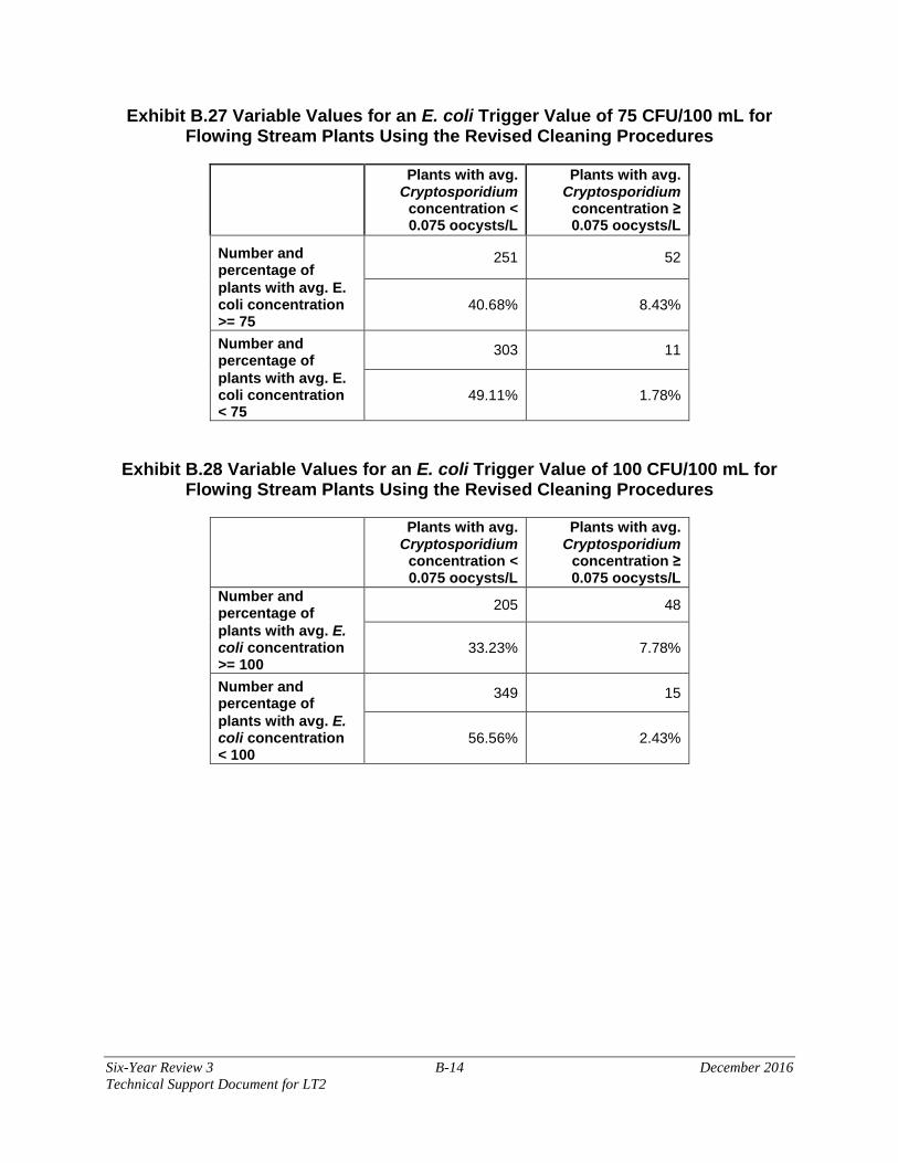
Six-Year Review 3 B-14 December 2016 Technical Support Document for LT2
Exhibit B.27 Variable Values for an E. coli Trigger Value of 75 CFU/100 mL for Flowing Stream Plants Using the Revised Cleaning Procedures
Plants with avg. Cryptosporidium
concentration < 0.075 oocysts/L
Plants with avg. Cryptosporidium
concentration ≥ 0.075 oocysts/L
Number and percentage of
251 52
plants with avg. E. coli concentration >= 75
40.68% 8.43%
Number and percentage of
303 11
plants with avg. E. coli concentration < 75
49.11% 1.78%
Exhibit B.28 Variable Values for an E. coli Trigger Value of 100 CFU/100 mL for Flowing Stream Plants Using the Revised Cleaning Procedures
Plants with avg. Cryptosporidium
concentration < 0.075 oocysts/L
Plants with avg. Cryptosporidium
concentration ≥ 0.075 oocysts/L
Number and percentage of 205 48
plants with avg. E. coli concentration >= 100
33.23% 7.78%
Number and percentage of
349 15
plants with avg. E. coli concentration < 100
56.56% 2.43%

Six-Year Review 3 B-15 December 2016 Technical Support Document for LT2
Exhibit B.29 Variable Values for an E. coli Trigger Value of 150 CFU/100 mL for Flowing Stream Plants Using the Revised Cleaning Procedures
Plants with avg. Cryptosporidium
concentration < 0.075 oocysts/L
Plants with avg. Cryptosporidium
concentration ≥ 0.075 oocysts/L
Number and percentage of 169 40
plants with avg. E. coli concentration >= 150
27.39% 6.48%
Number and percentage of
385 23
plants with avg. E. coli concentration < 150
62.40% 3.73%
Exhibit B.30 Variable Values for an E. coli Trigger Value of 200 CFU/100 mL for Flowing Stream Plants Using the Revised Cleaning Procedures
Plants with avg. Cryptosporidium
concentration < 0.075 oocysts/L
Plants with avg. Cryptosporidium
concentration ≥ 0.075 oocysts/L
Number and percentage of 133 38
plants with avg. E. coli concentration >= 200
21.56% 6.16%
Number and percentage of 421 25
plants with avg. E. coli concentration < 200
68.23% 4.05%

Six-Year Review 3 B-16 December 2016 Technical Support Document for LT2
Exhibit B.31 through Exhibit B.36 show the variables for plants categorized as both reservoir/lake and flowing stream using the revised cleaning procedures.
Exhibit B.31 Variable Values for an E. coli Trigger Value of 10 CFU/100 mL for Plants Categorized as Both Using the Revised Cleaning Procedures
Plants with avg. Cryptosporidium
concentration < 0.075 oocysts/L
Plants with avg. Cryptosporidium
concentration ≥ 0.075 oocysts/L
Number and percentage of 30 5
plants with avg. E. coli concentration >= 10
56.60% 9.43%
Number and percentage of 17 1
plants with avg. E. coli concentration < 10
32.08% 1.89%
Exhibit B.32 Variable Values for an E. coli Trigger Value of 50 CFU/100 mL for Plants Categorized as Both Using the Revised Cleaning Procedures
Plants with avg. Cryptosporidium
concentration < 0.075 oocysts/L
Plants with avg. Cryptosporidium
concentration ≥ 0.075 oocysts/L
Number and percentage of 12 3
plants with avg. E. coli concentration >= 50
22.64% 5.66%
Number and percentage of 35 3
plants with avg. E. coli concentration < 50
66.04% 5.66%

Six-Year Review 3 B-17 December 2016 Technical Support Document for LT2
Exhibit B.33 Variable Values for an E. coli Trigger Value of 75 CFU/100 mL for Plants Categorized as Both Using the Revised Cleaning Procedures
Plants with avg. Cryptosporidium
concentration < 0.075 oocysts/L
Plants with avg. Cryptosporidium
concentration ≥ 0.075 oocysts/L
Number and percentage of 8 3
plants with avg. E. coli concentration >= 75
15.09% 5.66%
Number and percentage of
39 3
plants with avg. E. coli concentration < 75
73.58% 5.66%
Exhibit B.34 Variable Values for an E. coli Trigger Value of 100 CFU/100 mL for Plants Categorized as Both Using the Revised Cleaning Procedures
Plants with avg. Cryptosporidium
concentration < 0.075 oocysts/L
Plants with avg. Cryptosporidium
concentration ≥ 0.075 oocysts/L
Number and percentage of 6 3
plants with avg. E. coli concentration >= 100
11.32% 5.66%
Number and percentage of
41 3
plants with avg. E. coli concentration < 100
77.36% 5.66%

Six-Year Review 3 B-18 December 2016 Technical Support Document for LT2
Exhibit B.35 Variable Values for an E. coli Trigger Value of 150 CFU/100 mL for Plants Categorized as Both Using the Revised Cleaning Procedures
Plants with avg. Cryptosporidium
concentration < 0.075 oocysts/L
Plants with avg. Cryptosporidium
concentration ≥ 0.075 oocysts/L
Number and percentage of 6 3
plants with avg. E. coli concentration >= 150
11.32% 5.66%
Number and percentage of 41 3
plants with avg. E. coli concentration < 150
77.36% 5.66%
Exhibit B.36 Variable Values for an E. coli Trigger Value of 200 CFU/100 mL for Plants Categorized as Both Using the Revised Cleaning Procedures
Plants with avg. Cryptosporidium
concentration < 0.075 oocysts/L
Plants with avg. Cryptosporidium
concentration ≥ 0.075 oocysts/L
Number and percentage of
4 2
plants with avg. E. coli concentration >= 200
7.55% 3.77%
Number and percentage of 43 4
plants with avg. E. coli concentration < 200
81.13% 7.55%

Six-Year Review 3 B-19 December 2016 Technical Support Document for LT2
Exhibit B.37 through Exhibit B.42 show the variable values for all plants using the revised cleaning procedures.
Exhibit B.37 Variable Values for an E. coli Trigger Value of 10 CFU/100 mL for All Plants Using the Revised Cleaning Procedures
Plants with avg. Cryptosporidium
concentration < 0.075 oocysts/L
Plants with avg. Cryptosporidium
concentration ≥ 0.075 oocysts/L
Number and percentage of 806 86
plants with avg. E. coli concentration >= 10
58.75% 6.27%
Number and percentage of 476 4
plants with avg. E. coli concentration < 10
34.69% 0.29%
Exhibit B.38 Variable Values for an E. coli Trigger Value of 50 CFU/100 mL for All Plants Using the Revised Cleaning Procedures
Plants with avg. Cryptosporidium
concentration < 0.075 oocysts/L
Plants with avg. Cryptosporidium
concentration ≥ 0.075 oocysts/L
Number and percentage of 430 69
plants with avg. E. coli concentration >= 50
31.34% 5.03%
Number and percentage of 852 21
plants with avg. E. coli concentration < 50
62.10% 1.53%

Six-Year Review 3 B-20 December 2016 Technical Support Document for LT2
Exhibit B.39 Variable Values for an E. coli Trigger Value of 75 CFU/100 mL for All Plants Using the Revised Cleaning Procedures
Plants with avg. Cryptosporidium
concentration < 0.075 oocysts/L
Plants with avg. Cryptosporidium
concentration ≥ 0.075 oocysts/L
Number and percentage of 351 65
plants with avg. E. coli concentration >= 75
25.58% 4.74%
Number and percentage of 931 25
plants with avg. E. coli concentration < 75
67.86% 1.82%
Exhibit B.40 Variable Values for an E. coli Trigger Value of 100 CFU/100 mL for All Plants Using the Revised Cleaning Procedures
Plants with avg. Cryptosporidium
concentration < 0.075 oocysts/L
Plants with avg. Cryptosporidium
concentration ≥ 0.075 oocysts/L
Number and percentage of
279 59
plants with avg. E. coli concentration >= 100
20.34% 4.30%
Number and percentage of 1,003 31
plants with avg. E. coli concentration < 100
73.10% 2.26%

Six-Year Review 3 B-21 December 2016 Technical Support Document for LT2
Exhibit B.41 Variable Values for an E. coli Trigger Value of 150 CFU/100 mL for All Plants Using the Revised Cleaning Procedures
Plants with avg. Cryptosporidium
concentration < 0.075 oocysts/L
Plants with avg. Cryptosporidium
concentration ≥ 0.075 oocysts/L
Number and percentage of 211 47
plants with avg. E. coli concentration >= 150
15.38% 3.43%
Number and percentage of 1,071 43
plants with avg. E. coli concentration < 150
78.06% 3.13%
Exhibit B.42 Variable Values for an E. coli Trigger Value of 200 CFU/100 mL for All Plants Using the Revised Cleaning Procedures
Plants with avg. Cryptosporidium
concentration < 0.075 oocysts/L
Plants with avg. Cryptosporidium
concentration ≥ 0.075 oocysts/L
Number and percentage of 156 44
plants with avg. E. coli concentration >= 200
11.37% 3.21%
Number and percentage of 1,126 46
plants with avg. E. coli concentration < 200
82.07% 3.35%

Six-Year Review 3 Technical Support Document for LT2 December 2016
Appendix C
Toolbox Option Usage and Related Implementation Issues

Six-Year Review 3 Technical Support Document for LT2 C-1 December 2016
Exhibit C.1 presents the LT2 toolbox options and the number of systems using each option as of May 2013. Exhibit C.1 includes systems that have been placed in Bin 2 or higher based on their Cryptosporidium monitoring results, and are therefore required to install at least one toolbox technology.
Data on the number of systems using each toolbox option was provided by EPA Regional offices and the Association of State Drinking Water Administrators (ASDWA), findings from web searches, and results of a detailed literature review. On some occasions during the gathering of information, it was not absolutely clear whether systems were implementing toolbox technologies to comply with the LT2 or whether they were installing the technologies for other reasons.
Note that individual water systems have frequently opted to implement more than one toolbox technology (e.g., membrane filtration combined with ultraviolet (UV) disinfection). Toolbox technologies that have not been selected by the systems (for which EPA has collected information) are not listed in Exhibit C.1. Exhibit C.1 also provides brief summaries of implementation challenges and concerns that are related to the particular toolbox option, as discussed in the main body of this report.

Six-Year Review 3 C-2 December 2016 Technical Support Document for LT2
Exhibit C.1 Systems in Bin 2 or Higher: Summary of the Number of Systems Applying Toolbox Options and Related Implementation Challenges and Concerns
Toolbox Option Credits Currently Allowed
Number of Systems Using
the Option1
% of Systems Selecting
Toolbox Option Implementation Challenges and Concerns
Source Protection and Management Toolbox Options
Watershed Control Program (WCP) 0.5-log credit 11 6.6%
Few systems have chosen this option due to: • Tight time schedule and time-consuming efforts
needed for development and implementation, • Stringent elements required for the watershed
control plan, and • Relatively low removal credit available through
this option. Alternative Source / Intake Management
No prescribed credit 7 4.2% Tight time schedule and time-consuming efforts needed for development and implementation into existing treatment processes
Pre-Filtration Toolbox Options Pre-Sedimentation Basin with Coagulation
0.5-log credit: 2 1.2%
Time-consuming efforts needed for development and implementation
Two-stage Lime Softening
0.5-log credit 1 0.6%
Time-consuming efforts needed for development and implementation
Bank Filtration (BF)
0.5-log credit for 25-foot setback; 1.0-log credit for 50-foot setback; Additional credit for state-approved site specific study
4 2.4%
The implementation issue identified is the difficulty demonstrating more than 2-log Cryptosporidium removal credit using bank filtration

Six-Year Review 3 C-3 December 2016 Technical Support Document for LT2
Toolbox Option Credits Currently Allowed
Number of Systems Using
the Option1
% of Systems Selecting
Toolbox Option Implementation Challenges and Concerns
Treatment Performance Toolbox Options
Combined Filter Performance 0.5-log credit 43 25.9%
Concerns related to data and reporting integrity, accuracy of the tool and the oversight necessary to ensure the validity of the credit over time
Individual Filter Performance 0.5-log credit 39 23.5%
Concerns related to data and reporting integrity, accuracy of the tool and the oversight necessary to ensure the validity of the credit over time
Demonstration of Performance (DOP)
Credit awarded to unit process or treatment train based on a demonstration to the state with a state-approved protocol. [40 CFR 141.718 (c)]
3 1.8%
Issues raised include: • It is unclear if states have developed DOP
protocols and whether they are made available to the public;
• EPA’s Toolbox Guidance Manual introducesbasic DOP concepts but, without state-developed protocols issued in a timely manner, a system would not be aware of all the required elements to include in the DOP or length of time needed for the study (e.g., pilot test), and;
• Meeting the schedule for LT2 compliance mayhave been a contributing factor for systems not selecting this option.
Filtration2 (Option Unknown) 12 7.2%
Additional Filtration Toolbox Options
Bag and Cartridge Filters
Up to 2-log credit if used singly; Up to 2.5 log credit if in series.
13 0.6% Challenge testing determination may be a deterrent
Membrane Filtration
Log credit equivalent to removal efficiency demonstrated in challenge test for device if supported by direct integrity testing. [40 CFR 141.719(b)]
18 10.8%
Issues raised include: • New technologies such as ceramic membranes
have entered the water treatment market, and • There is a lack of data and a consensus on
how to use the data in evaluating membrane applications.

Six-Year Review 3 C-4 December 2016 Technical Support Document for LT2
Toolbox Option Credits Currently Allowed
Number of Systems Using
the Option1
% of Systems Selecting
Toolbox Option Implementation Challenges and Concerns
Second Stage Filtration 0.5-log credit 2 1.2% Implementation requires a large capital investment
Inactivation Toolbox Options
Chlorine Dioxide
Log credit based on measured CT in relation to CT table. [40 CFR 141.720 (b)]
1 0.6% Implementation requirements of ongoing monitoring, sampling and analysis
Ozone
Log credit based on measured CT in relation to CT table. [40 CFR 141.720 (b)]
3 1.8%
Documented operational issues include: • Operating costs,• Bromate formation may preclude the use of
ozone, and• Practicality of calculating CT is limited.
UV disinfection
Log credit based on validated UV dose in relation to UV dose table; reactor validation testing required to establish UV does and associated operating conditions. [40 CFR 141.720 (d)]
19 11.4%
Documented operational issues include: • Monitoring of UV dose delivered,• Verifying inactivation for viruses,• How to verify pre-existing UV installations meet
Cryptosporidium inactivation requirements,• Maintenance of reactors, and• Operating costs.
Total Number of Applied Toolbox Options 166 100% Notes:
1) Systems may be counted more than once if they use multiple toolbox options. In addition, not every applied toolbox option is for LT2 compliance.2) Available data describes use of a filtration process only but does not describe which toolbox option (combined filter performance, individual filter
performance or DOP) the system used for credits.3) Available data indicates bag and/or cartridge filters only and does not provide information related to whether they are individual filters or filters operating in
series.