Sliced Inverse Regression for Dimension ReductionKER-CHAU U*

Modem advances in computing power have greatly widened scientists' scope in gathering and investigating information frommany variables, information which might have been ignored in the past. Yet to effectively scan a large pool of variables is notan easy task, although our ability to interact with data has been much enhanced by recent innovations in dynamic graphics. Inthis article, we propose a novel data-analytic tool, sliced inverse regression (SIR), for reducing the dimension of the input variablex without going through any parametric or nonparametric model-fitting process. This method explores the simplicity of theinverse view of regression; that is, instead of regressing the univariate output variable y against the multivariate x, we regressx against y. Forward regression and inverse regression are connected by a theorem that motivates this method. The theoreticalproperties of SIR are investigated under a model of the form, y = j({3,x, ... , {3KX, e), where the {3;s are the unknown rowvectors. This model looks like a nonlinear regression, except for the crucial difference that the functional form ofjis completelyunknown. For effectively reducing the dimension, we need only to estimate the space [effective dimension reduction (e.d.r.)space] generated by the {3;s. This makes our goal different from the usual one in regression analysis, the estimation of all theregression coefficients. In fact, the {3;s themselves are not identifiable without a specific structural form onj. Our main theoremshows that under a suitable condition, if the distribution of x has been standardized to have the zero mean and the identitycovariance, the inverse regression curve, E(x Iy), will fall into the e.d.r. space. Hence a principal component analysis on thecovariance matrix for the estimated inverse regression curve can be conducted to locate its main orientation, yielding our estimatesfor e.d.r. directions. Furthermore, we use a simple step function to estimate the inverse regression curve. No complicatedsmoothing is needed. SIR can be easily implemented on personal computers. By simulation, we demonstrate how SIR caneffectively reduce the dimension of the input variable from, say, 10 to K = 2 for a data set with 400 observations. The spin-plot of y against the two projected variables obtained by SIR is found to mimic the spin-plot of y against the true directionsvery well. A chi-squared statistic is proposed to address the issue of whether or not a direction found by SIR is spurious.

KEY WORDS: Dynamic graphics; Principal component analysis; Projection pursuit.

1. INTRODUCTION

Regression analysis is a popular way of studying the re-lationship between a response variable y and its explanatoryvariable x, a p-dimensional column vector. Quite often, aparametric model is used to guide the analysis. When themodel is parsimonious, standard estimation techniques suchas the maximum likelihood or the least squares method haveproved to be successful in gathering information from thedata.In most applications, however, any parametric model is

at best an approximation to the true one, and the search foran adequate model is not easy. When there are no persua-sive models available, nonparametric regression techniquesemerge as promising alternatives that offer the needed flex-ibility in modeling. A common theme of nonparametricregression is the idea of local smoothing, which exploresonly the continuity or differentiability property of the trueregression function. The success of local smoothing hingeson the presence of sufficiently many data points around eachpoint of interest in the design space to provide adequateinformation. For one-dimensional problems, many smooth-

* Ker-Chau Li is Professor, Division of Statistics, Department of Math-ematics, University of California, Los Angeles, CA 90024. This researchwas supported in part by the National Science Foundation under grantsDMS86-02018 and DMS89-02494. It has been a long time since I intro-duced SIR in talks given at Berkeley, Bell Labs, and Rutgers in 1985. Ireceived many useful questions and suggestions from these audiences. Iam indebted to Naihua Duan for stimulating more ideas for improvement,leading eventually to Duan and Li (1991). Peter Bickel brought semi-parametric literature to my attention. Jan de Leeuw broadened my knowl-edge in areas of dimension reduction and multivariate analysis. WithoutDennis Cook, who introduced XLISP-STAT to me, the appearance ofSection 6.3 would have been further delayed. As a replacement for "sliceregression" or "slicing regression," used earlier, the name SIR was sug-gested to me by Don Ylvisaker, who also helped me clear hurdles inpublishing this article. Three referees and an associate editor offered nicesuggestions for improving the presentation. Finally, I would like to thankDavid Brillinger, whose work has inspired me so much.

ing techniques are available (see Eubank 1988 for a com-prehensive account).As the dimension of x gets higher, however, the total

number of observations needed for local smoothing esca-lates exponentially. Unless we have a gigantic sample,standard methods, such as kernel estimates or nearest-neighbor estimates, break down quickly because of thesparseness of the data points in any region of interest. Tochallenge the curse of dimensionality, one hope that stat-isticians may capitalize on is that interesting features of high-dimensional data are retrievable from low-dimensional pro-jections. For regression problems, the following model de-scribes such an ideal situation:

(1.1)

Here the {3's are unknown row vectors, E is independent ofx, and j' is an arbitrary unknown function on RK+1•When this model holds (cf. Remark 1.1), the projection

of the p-dimensional explanatory variable x onto the K di-mensional subspace, ({31X, ... , (3KX) , , captures all we needto know about y. When K is small, we may achieve thegoal of data reduction by estimating the {3's efficiently. Forconvenience, we shall refer to any linear combination ofthe {3's as an effective dimension-reduction (e.d.r.) direc-tion, and to the linear space B generated by the {3's as thee.d.r. space. More discussion on this model, e.d.r. direc-tions, and the relation to other approaches is given in Sec-tion 2. Our main focus in this article is on the estimationof the e.d.r. directions, leaving questions such as how toestimate main features of / for further investigation. Intu-itively speaking, after estimating the e.d.r. directions, stan-dard smoothing techniques can be more successful because

© 1991 American Statistical AssociationJoumal of the American Statistical Association

June 1991. Vol. 86. No. 414, Theory and Methods

316

Dow

nloa

ded

by [S

hang

hai J

iaot

ong

Uni

vers

ity] a

t 17:

16 2

2 M

ay 2

016

Li: Sliced Inverse Regression

the dimension has been lowered (cf. Remark 1.2). On theother hand, during the exploratory stage of data analysis,one often wants to view the data directly. Many graphicaltools are available (see, for instance, the special applica-tions section on statistical graphics, introduced by Cleve-land 1987), but plotting y against every combination of xwithin a reasonable amount of time is impossible. So, touse the scatterplot-matrix techniques (Carr et al. 1987), weoften focus on coordinate variables only. Likewise, 3-D ro-tating plots (e.g., see Huber 1987) can handle only onetwo-dimensional projection of x at a time (the third dimen-sion is reserved for y). Therefore, to take full advantage ofmodem graphical tools, guidance on how to select the pro-jection directions is clearly called for. A good estimate ofthe e.d.r. directions can lead to a good view of the data.Section 6.3 demonstrates how sharp the view found by ourmethod is.Our method of estimating the e.d.r. directions is based

on the idea of inverse regression. Instead of regressing yagainst x (forward regression) directly, we regress x againsty (inverse regression). The immediate benefit for exchang-ing the roles of y and x is that we can side-step the di-mensionality problem. This comes out because inverseregression can be carried out by regressing each coordinateof x against y. Thus we essentially deal with a one-dimen-sion to one-dimension regression problem, rather than thehigh-dimensional forward regression.The feasibility of finding the e.d.r. directions via inverse

regression will become clear. As y varies, E(x I y) drawsa curve, called the inverse regression curve, in RP. Under(1.1), however, this curve typically will hover around a K-dimensional affine subspace. At one extreme, as shown inTheorem 3.1 of Section 3, the inverse regression curve ac-tually falls into a K-dimensional affine subspace determinedby the e.d.r. directions, provided that the distribution of xsatisfies (3.1). If we have standardized x to have mean 0and the identity covariance, then this subspace coincideswith the e.d.r. space. Elliptically symmetric distributions,including the normal distribution, satisfy condition (3.1).Exploring the simplicity of inverse regression, we de-

velop a simple algorithm, called sliced inverse regression(SIR), for estimating the e.d.r. directions. After standard-izing x, SIR proceeds with a crude estimate of the inverseregression curve E(x Iy), which is the slice mean of x afterslicing the range of y into several intervals and partitioningthe whole data into several slices according to the y value.A principal component analysis is then applied to these slicemeans of x, locating the most important K-dimensionalsubspace for tracking the inverse regression curve E(x Iy).The output of SIR is these components after an affine re-transformation back to the original scale.In Section 5, under the design condition of (3.1), we show

that SIR yields root n consistent estimates for the e.d.r.directions.Besides offering estimates of e.d.r. directions, the out-

puts of SIR are themselves interesting descriptive statisticscontaining useful information about the inverse regressioncurve. In Section 7, we elaborate this point further and ar-gue that the directions produced by SIR can be used to form

317

variables (derivable from x linearly) that are most predict-able from y. Thus for graphical purposes, even if the designcondition (3.1) is not satisfied, SIR still suggests interestingdirections for viewing the data.As a sharp contrast to most nonparametric techniques that

require intensive computation, SIR is very simple to im-plement. Moreover, the sampling property of SIR is easyto understand, another advantage over other methods. Thusit is possible to assess the effectiveness of SIR by using thecompanion output eigenvalues at the principal componentanalysis step (see Remark 5.1 in Section 5). These eigen-values provide valuable information for assessing the num-ber of components in the data (see Remark 5.2). Finally,selection of the number of slices for SIR is less crucial thanselection of the smoothing parameter for typical nonpara-metric regression problems. We further illustrate these pointsby simulation in Section 6.In view of these virtues, however, SIR is not intended

to replace other computer-intensive methods. Rather it canbe used as a simple tool to aid other methods; for instance,it provides a good initial estimate for many methods basedon the forward regression viewpoint. Because of low com-puting cost, one should find it easy to incorporate SIR intomost statistical packages.

Remark 1.1. All models are imperfect in some senseand (1. 1) should be interpreted as an approximation to real-ity. However, there is a fundamental difference betweenthis and other statistical models: (1.1) takes the weakestform for reflecting our hope that a low-dimensional pro-jection of a high-dimensional regressor variable contains mostof the information that can be gathered from a sample of amodest size. Equation (1.1) does not impose any structureon how the projected regressor variable affects the outputvariable. In addition, we may even vary K to reflect thedegree of the anticipated dimension reduction. At K = p,(1.1) becomes a redundant assumption. By comparison, mostregression models assume K = 1, with additional structuresonf.

Remark 1.2. A philosophical point needs to be empha-sized here: The estimation of the projection angles can bea more important statistical issue than the estimation of thestructure off itself. In fact, the structure off is impossibleto identify unless we have other scientific evidence beyondthe data under study. One can obtain two different versionsof f to represent the same joint distribution of y and x [cf.(2.1)]. Thus what we can estimate are at most statisticalquantities, such as the conditional mean or quantiles of ygiven x. On the other hand, during the early stages of dataanalysis, when one does not have a fixed objective in mind,the need for estimating such quantities is not as pressing asthat for finding ways to simplify the data. Our formulationof estimating the e.d.r. directions is one way to addresssuch a need in data analysis. After finding a good e.d.r.space, we can project data into this smaller space. We arethen in a better position to identify what should be pursuedfurther: model building, response surface estimation, clus-ter analysis, heteroscedasticity analysis, variable selection,or inspecting scatterplots (or spin-plots) for interesting fea-

Dow

nloa

ded

by [S

hang

hai J

iaot

ong

Uni

vers

ity] a

t 17:

16 2

2 M

ay 2

016

318 Journal of the American Statistical Association, June 1991

the squared multiple correlation coefficient between theprojected variable bx and the ideally reduced variables f31X,.•. , f3KX. For a collection of K estimated directions b l , ... ,bK generating a linear subspace B,we use the squared trace

ger's result to a general class of maximum likelihood typeestimators.Turning to the multicomponent model (K> 1), observe

that the conditional expectation E(y I x), the forwardregression surface, takes the form g(f3lx, ... , f3Kx). Fromthe forward regression viewpoint, after projecting x ontoany K-dimensional subspace (with a basis, say, bi, ... , bK ) ,

it is possible to estimate the conditional expectation E( y Ibkx's) nonparametrically. The average conditional varianceE[var(y I bkx's)] is minimized when the projection spacecoincides with the space of the e.d.r. directions. We areled to a variant of the projection pursuit method studied inChen (in press), which estimates the e.d.r. space by glob-ally searching for a best K-dimensional projection that min-imizes a lack-of-fit measure based on the residual sum ofsquares. Large-sample results were derived, but the methodappears to be highly computer-intensive because one has toworry not only about how to do a global search efficientlybut also about how to do the multidimensional smoothing.If the conditional expectation E(y Ix) takes the additivity

form, gl(f3lx) + ... + gK(f3KX), then one may use the pro-jection pursuit regression algorithm (PPR) as described inFriedman and Stuetzle (1981) to estimate the e.d.r. direc-tions. Donoho and Johnstone (1989), Hall (1989), and Huber(1985) add more insight to PPR.Another possible forward regression route to attack this

problem is based on the observation that under (1.1), anyslope vector, the derivative of y with respect to x at anypoint, falls within the e.d.r. space B. Thus if we can es-timate the slope vectors well, we may apply a principalcomponent analysis to the estimated slope vectors to findthe e.d.r. directions. The main difficulty for this approach,however, is the estimation of the derivatives for highdimensional x.Many recent works are related to data reduction. A short

and incomplete list includes the correspondence analysisapproach (e.g., van Rijckevorsel and de Leeuw 1988),classification trees (e.g., Breiman, Friedman, Olshen, andStone 1984; Loh and Vanichsetakul 1988), ACE and ad-ditive models (Breiman and Friedman 1985; Koyak 1987;Stone 1986), and partial spline models (Chen 1988; Cuzick1987; Engle et al. 1983; Heckman 1986; Speckman 1987;Wahba 1986), and projection pursuit density estimation (e.g.,Diaconis and Freedman 1984; Friedman 1987; Huber 1985).We conclude this section by discussing the question of

how to evaluate the effectiveness of an estimated e.d.r. di-rection. An obvious criterion is based on the squared Eu-clidean distance between the estimated e.d.r. direction b(normalized to have the unitary length) and the true e.d.r.space B. This criterion, however, is not invariant under scalechange or affine transformation of x. We prefer an affineinvariant criterion,

tures. This approach toward data analysis is different fromthat in many other works. Projection pursuit regression(Friedman and Stuetzle 1981), ACE and additive models(Breiman and Friedman 1985; Stone 1986; Hastie and Tib-shirani 1986), or partial splines (Chen 1988b; Cuzik 1987;Engle, Granger, Rice, and Rice 1986; Heckman 1986;Speckman 1987; Wahba 1986), for instance, seem to havesingled out the approximation of the conditional mean ofthe output variable (or its transformation) as their primarygoal. But dimension reduction in statistics has a wider scopethan functional approximation. The concept of e.d.r. spaceand the method of SIR aim at this general purpose of di-mension reduction.After dimension reduction, if we want to estimate the

response surface, for example, we can apply standard tech-niques in nonparametric regression to the projected vari-ables (e.g. Li 1987 and the references therein). In addition,suitable conditional influence as in the Box-Cox transfor-mation study (Hinkley and Runger 1984) may be valuable.Needless to say, the door is open for further serious work.

2. A MODEL FOR DIMENSION REDUCTION

Equation (1.1) describes an ideal situation where one canreduce the dimension of the explanatory variable from p toa smaller number K without losing any information. Anequivalent version of (1.1) is: The conditional distributionof y given x depends on x only through the K dimensionalvariable (f3IX, ... , f3Kx ). Thus conditional on f3kX'S, y andx are independent; the perfectly reduced variable, (f3IX, ... ,f3KX) , is seen to be as informative as the original x in pre-dicting y.Recall the terminology of e.d.r. direction and e.d.r. space

from Section 1. Observe that by changing f suitably, (1.1)can be reparameterized by any set of K linearly independente.d.r. directions. Another interpretation is that conditioningon (f3IX, ... , f3Kx) is equivalent to conditioning on any non-degenerate affine transformation of this vector. Thus it isthe e.d.r. space B that can be identified; the individual vec-tors f3h ... , 13K are not themselves identifiable (unless fur-ther structural conditions on f are imposed).Let I xx be the covariance matrix of x. Later on, we shall

find it convenient to consider the standardized version ofx, z = '£;".1/2 [x - E(x)]. We may rewrite (1.1) as

(2.1)

where 11k = (k = 1, ... , K). We shall call any vectorin the linear space generated by the 11k'S a standardized e.d.r.direction.We will discuss the relationship of our model to others

subsequently.First of all, it is fair to say that one-component models

(K = 1) prevail in the literature; for instance, the gener-alized linear model, the Box-Cox transformation model andits generalization (Box and Cox 1964; Bickel and Doksum1981; Carroll and Ruppert 1984) and others. Brillinger (1977,1983) derived a surprising result about the robustness ofleast squares estimation under a global misspecification ofthe link function. Li and Duan (1989) generalized Brillin-

(bIxxf3')2R2(b) = max -'------==----'-----

{3EB bIxxb' f3Ixxf3"(2.2)

Dow

nloa

ded

by [S

hang

hai J

iaot

ong

Uni

vers

ity] a

t 17:

16 2

2 M

ay 2

016

Li: Sliced Inverse Regression

correlation, denoted by R2(B ) , as our criterion: the averageof the squared canonical correlation coefficients betweenbvx, ... , bKx and {3jX, ... , {3KX (Hooper 1959). It is alsoreasonable to replace lxx by the sample covariance matrixin our definition of the criteria.

3. THE INVERSE REGRESSION CURVEConsider the trajectory of the inverse regression curve

E(x I y) as y varies. The center of this curve is located atE(E(x Iy» = E(x). In general, the centered inverse regres-sion curve, E(x I y) - E(x) is a p-dimensional curve inW. We shall see that it lies on a K-dimensional subspace,however, with the following condition on the designdistribution:

Condition 3.1. For any b in RP, the conditional expec-tation E(bx I{3\x, ... , (3KX) is linear in {3\x, ... , {3KX; thatis, for some constants Co, C1, ... , CK, E(bx I{3\x, ... , (3KX)= Co + c\{3\x + ... + CK{3KX.

This condition is satisfied when the distribution of x iselliptically symmetric (e.g., the normal distribution). Morediscussion of this condition is given in Remark 3.3. Thefollowing theorem will be proved in the Appendix.

Theorem 3.1 . Under the conditions (1.1) and (3.1), thecentered inverse regression curve E(x I y) - E(x) is con-tained in the linear subspace spanned by {3klxx (k = 1, ... ,K), where lxx denotes the covariance matrix of x.Corollary 3.1. Assume that x has been standardized to

z. Then under (2.1) and (3.1), the standardized inverseregression curve E(z I y) is contained in the linear spacegenerated by the standardized e.d.r. directions 111> ... , 11K'

An important consequence of this corollary is that thecovariance matrix cov[E(z Iy)] is degenerate in any direc-tion orthogonal to the 11k'S. We see, therefore, that the ei-genvectors, l1k(k = 1, ... , K), associated with the largestK eigenvalues of cov[E(z I y)] are the standardized e.d.r.directions. Transforming back to the original scale,l1kl-\/2 (k = 1, ... , K) are in the e.d.r. space. This leadsto the SIR algorithm of the next section.

Remark 3.1. Conditional covariance cov(z Iy) can alsoreveal valuable clues for finding the standardized e.d.r. di-rections. To see this, simply observe the identity

E[cov(z Iy)] = cov z - cov[E(z Iy)] = I - cov[E(z Iy)].Therefore, after an eigenvalue decomposition of E[cov(z Iy)], we may find the standardized e.d.r. directions from theeigenvectors associated with the smallest K eigenvalues. Theestimation of E[cov(z Iy)] is not difficult; see Remark 5.3.Remark 3.2. Regression models are usually formed by

decomposing the joint distribution of y and x as h( y Ix)k(x)and modeling h(y Ix). This is the forward view of regres-sion. The inverse view of regression factorizes the jointdensity as h(x Iy)k(y) and models h(x Iy). Important casesof inverse formation include discriminant analysis (with lo-gistic regression as the counterpart from the forward view).SIR is itself meaningful from the inverse view of modeling.

319

It is interesting to observe that we may consider y as a pa-rameter with an empirical Bayes prior.

Remark 3.3. Condition (3.1) seems to impose a strin-gent requirement on the distribution of x. One implicationis that, at the stage of data collection, unless the functionalform of the response surface is known, we had best designthe experiment so that the distribution of x will not blatantlyviolate elliptic symmetry. For example, rotatable designs,advocated by George Box (see, e.g., Box and Draper 1987)in the response surface literature, deserve to be studied moreclosely in the future. On the other hand, after data collec-tion, it would help the analysis if closer examination of thedistribution of x can be made so that outliers can be re-moved or clusters can be separated before analysis.An interesting extension of Corollary 3.1 will be to quan-

tify how far away from the standardized e.d.r. space theinverse regression curve E(z I y) is when (3.1) is mildlyviolated. If the projection of E(z Iy) on the orthogonal com-plement of the standardized e.d.r. space is small, then thedirections picked up by the principal component analysison cov[E(z Iy)] will still be close to the standardized e.d.r.directions. The situation is similar to that in Brillinger (1977,1983) where consistency of least squares in estimating {3\for one-component models under (3.1) is proved. Further-more, empirical evidence was reported indicating that hisresult is not sensitive to violation of (3.1). A comprehen-sive account of this robustness issue for the least squaresand other commonly used regression estimates is given inLi and Duan (1989).After the first version of our article was written, this de-

sign robustness issue was further addressed in three articles.First, a bound to bias in estimation was obtained in Duanand Li (in press) for K = 1. Moreover, Li (1989) arguedthat for most directions b, we can expect the linearity in(3.1) to hold approximately, borrowing a powerful resultfrom Diaconis and Freedman (1984) where they showedthat most low-dimension projections of a high-dimensiondata cloud are close to being normal. Li (1989) also dem-onstrated how SIR may find the directions that violate (3.1)most seriously. Li (1990b) extended the discussion to aframework for the uncertainty analysis of mathematicalmodels.

4. SLICED INVERSE REGRESSIONA scheme for sliced inverse regression operates on the

data (Yi' Xi) (i = 1, ... , n), in the following way:

1. Standardize x by an affine transformation to get Xi =I;,.1/2 (Xi - x) (i = 1, ... , n), where s, and x are thesample covariance matrix and sample mean of x respec-tively.2. Divide range of y into H slices, II> ... , 1H ; let the

proportion of the Yi that falls in slice h be Ph; that is Ph =(1ln) l)h(y;) , where l)h(Yi) takes the values 0 or 1 de-pending on whether Yi falls into the hth slice h or not.3. Within each slice, compute the sample mean of the

x/s, denoted by mh (h = 1, ... , H), so that mh = (1lnph)Xi'

4. Conduct a (weighted) principal component analysis

Dow

nloa

ded

by [S

hang

hai J

iaot

ong

Uni

vers

ity] a

t 17:

16 2

2 M

ay 2

016

320

for the data mh (h = 1, ... , H) in the following way: Formthe weighted covariance matrix V = then findthe eigenvalues and the eigenvectors for V.5. Let the K largest eigenvectors (row vectors) be iik (k

_ A _ A A -1/2 _- 1, ... , K). Output 13k - 11k!'"" (k - 1, ... , K).

Steps 2 and 3 produce a crude estimate of the standard-ized inverse regression curve E(z I y). Although it is fea-sible to use more sophisticated nonparametric regressionmethods such as kernel, nearest neighbor, or smoothingsplines to yield a better estimate of the inverse regressioncurve, we advocate only the method of slicing due to itssimplicity. Since we only need the main orientation (butnot any other detailed aspects) of the estimated curve, pos-sible gains due to smoothing are not likely to be substantial.The weighting adjustment for principal component anal-

ysis in Step 4 takes care of the case where there may beunequal sample sizes in different slices. The first K com-ponents locate the most important subspace to track thestandardized inverse regression curve E(z Iy). Finally, Step5 retransforms the scale back to the original one. Thuscan be used as estimates of the e.d.r. directions and thee.d.r. space B is estimated by E, the space generated bytheA few remarks about the actual implementation are in

order.

Remark 4.1. It is not necessary to transform each in-dividual Xi to Xi' All we need is to transform the slice meansbefore conducting the principal component analysis to savecomputing time. Let II be Ph(jh - X)(Xh - x)', whereXh denotes the sample mean of the x,' s in the hth slice. Thenthe are just the eigenvectors for the eigenvalue decom-position of II with respect to I"". Using the terminologyofMANOYA (e.g., Mardia, Kent, and Bibby 1979, chap.12), II describes the between-slice variation.

Remark 4.2. The range for each slice may be set tohave equal length; but in section 6, we prefer to allow itto vary so that the number of observations in each slice canbe as close to each other as possible.

Remark 4.3. The choice of the number of slices mayaffect the asymptotic variance of the output estimate. How-ever, the difference is not significant for practical samplesizes in our simulation study. This issue here is less criticalthan the choice of a smoothing parameter in nonparamet-ric regression. Theoretically an inappropriate choice ofsmoothing parameter in nonparametric regression or den-sity estimation may lead to a slower rate of convergence,while for our case we can still have root n consistency nomatter how H is chosen; see Remark 5.3 in Section 5. Fora comprehensive treatment of adaptive choice of smoothingparameter in nonparametric regression, see Li (1987), andHardIe, Hall, and Marron (1988).

Remark 4.4. When standardizing x, it is not necessaryto base the affine transformation on the sample mean andsample covariance matrix. Some robust versions of themmay be preferable (see Donoho, Johnstone, Rousseeuw, andStahe11985; Fill and Johnstone 1984; and Li and Chen 1985).

Joumal of the American Statistical Association, June 1991

At least we should downweight or cut out those influentialdesign points. But this issue is probably less crucial and isrelatively easy to handle because we are dealing with thedesign points that are under our control (even in the ob-servational study, we may screen out some bad design points;if the percentage of the remaining points is high enough wecan still have a good analysis). Note that the efficiency ofthe affine transformation is not the main concern becausewe need only a consistent estimate to make SIR work.

Remark 4.5. If the standardized inverse regression curvefalls within a proper subspace of the standardized e.d.r.space, then SIR cannot recover all e.d.r. directions. Forinstance, if y = g(13lx) + E for some symmetric functiong, and 13lx is also symmetric about 0, then E(x Iy) equals0, and is a poor estimate of 131' For handling such cases,one approach is to explore higher conditional moments ofX given y. For instance, if x is normal, then for any direc-tion bx orthogonal to the 13kx's, we see that var(bx Iy) re-mains invariant as y changes. In particular, for standardizedx, the eigenvectors of cov(x lyE I h ) with eigenvalues dif-ferent from 1 are in the e.d.r. space. Thus if an eigenvaluedecomposition on the sample covariance of the x;'s, de-noted as COYh s for each slice h is conducted, then we maycombine those eigenvectors with eigenvalues significantlydifferent from 1 from each slice in a suitable way to esti-mate 13k'S. Details on ways of combination are under in-vestigation. It is not always necessary to conduct the ei-genvalue decomposition separately for each slice, however.For instance, one may treat it as an approximation problemof fitting each COYh - 1 separately by a nonnegative def-inite matrix of rank K with the constraint that the fittedmatrices have a common range. Another second momentmethod and a method based on the notion of principal Hes-sian directions were suggested in Li (1989, 1990a). Morerecently, the author also learned that Cook and Weisberghave independently obtained some good estimates based onthe second moments.

5. SAMPLING PROPERTIESIn this section we present a brief argument to show how

the output of SIR provides root n consistent estimates forthe e.d.r. directions.Let Ph = Pr{y E h} and m, = E(z lyE I h) , where z

stands for the standardized x, as defined in Section 2. El-ementary probability theory shows that mh converges to m,at rate n- I/2. Let V be the matrix Clearly theweighted covariance V in Step (4) of SIR converges to Vat the root n rate. Consequently, the eigenvectors of V, iik(k = 1, ... , K), converge to the corresponding eigenvec-tors for Vat the root n rate. Now we use Corollary 3.1 andthe simple identity m, = E[E(z Iy) lyE I h] to see that thefirst K eigenvectors of V fall in the standardized e.d.r. space.Since I;,.I/2 converges to !';,.1/2, we see that each con-verges to an e.d.r. direction at rate root n.The case where the range of each slice varies in order to

ensure an even distribution of observations is related to thefollowing choice of intervals:

I h = (F;l«h - 1)/H), F;I(h/H)),

Dow

nloa

ded

by [S

hang

hai J

iaot

ong

Uni

vers

ity] a

t 17:

16 2

2 M

ay 2

016

(5.1)

Li: Sliced Inverse Regression

where Fy(-) is the cdf of y. The root n consistency resultstill holds.

Remark 5.1. It is possible to establish the asymptoticnormality of the f3k'S and to calculate the asymptotic co-variance matrices using the delta method as in Mallows(1961) or Tyler (1981). In the Appendix we show how tuapproximate the expectation of R2(B ) , the squared trace cor-relation between f3kX'S and f3kX'S (see the last paragraph ofsection 2). For the normal x, we have the following simpleapproximation:

E[R 2(B )] = 1-p - K (-1 + +n K k=\ Ak n

where Ak is the kth eigenvalue of V. A crude estimate ofthis quantity is given by substituting the kth largest eigen-value of 11 for Ak•Remark 5.2. To be really successful in picking up all

K dimensions for reduction, the inverse regression curvecannot be too straight. In other words, the first K eigen-values for V must be significantly different from zero com-pared to the sampling error. This can be checked by thecompanion output eigenvalues of 11 in Step (4) of the SIR.The asymptotic distribution of the average of the smallestp - K eigenvalues, denoted by A(P-K), for 11 can be derivedbased on perturbation theory for finite-dimensional spaces(Kato 1976, chapter 2). For normal x, we have the follow-ing result.

Theorem 5.1. If x is normally distributed, then n(p -K)A(P-K) follows a X2 distribution with (p - K)(H - K -1) df asymptotically.

We may use this result to give a conservative assessmentof the number of components in the model. Thus if therescaled A(p-k) is larger than the corresponding X

2 value (saythe 95th percentile), then we may infer that there are atleast k + 1 (significant) components in the model. For otherelliptically symmetric distributions, the result is more com-plicated. Although it is possible to estimate the asymptoticdistribution using some version of the bootstrap method, wefeel it is good enough to use the normal case result as aguideline to keep our procedure as simple as possible. Anoutline for the proof of the asymptotic result discussed hereis given in the Appendix. A referee pointed out the simi-larity between this result and the result of a likelihood ratiotest in MANOVA (Mardia et al. 1979, p. 342; further con-nection between SIR and sec. 12.5.4 of that reference canalso be drawn). We remind the reader, however, that thefundamental assumption about the error distribution inMANOVA is not satisfied for our case. The conditionaldistribution of x given y is not normal, even if x is normalunconditionally. Furthermore, the conditional variance of xgiven y E Ih depends on h. Hence one has to be very carefulif linking of SIR with MANOVA is desired.

Remark 5.3. Can SIR still yield reasonable estimates ifthe number of slices increases too fast and the number ofobservations in each slice is too small for 11th to consistentlyestimate mh? Remark 3.1 offers an answer. First, we see

321

that the following is one way to estimate E[cov(z Iy)]:(a) Introduce a large number of slices for partitioning the

range of y.(b) Within each slice, form the sample covariance ofx;'s

that fall into that slice.(c) Form an average of the estimated conditional co-

variances of (b).

Intuitively, in order to get rid of the bias for estimating theconditional variance cov(z I y) for each y in (b), we hopethat the range of each slice will converge to 0, so that onlylocal points will contribute to the estimation. But when thenumber of slices is too large, the sampling variance in eachestimate of cov(z I y) may not diminish, even for large n.Fortunately, the averaging process of (c) will stabilize thefinal estimate by the law of large numbers. As a matter offact, even if the slice number is n/2, so that each slicecontains only two observations, the resulting estimate willstill be root n consistent.The interesting connection of this estimate of E[cov(z I

y)] to SIR is that this estimate is proportional to I - 11because of the sample version of the identity given in Re-mark 3.1. Because of this conjugate relationship, a prin-cipal component analysis on the above estimate of E[cov(zIy)] for the smallest K components is equivalent to a prin-cipal component analysis on 11 for the largest K compo-nents. This explains why a large number of slices may stillwork, bolstering our earlier .claim that the selection of His not as crucial as the choice of a smoothing parameterin most nonparametric regression or density estimationproblems.

Remark 5 .4. It is interesting to study the asymptotic be-havior of the SIR estimate when both the sample size andthe dimension p of x increase simultaneously, but the num-ber of components K and the number of slices H are keptfixed. One can see that a sufficient condition for the fik toconverge to TJk (in the sense that the angle between the twoconverges to 0) in probability is that the maximum singularvalue for 11 - V converges to 0 in probability. When theeigenvalues of V are bounded away from 0 and infinity asn increases, the above sufficient condition is implied by thecondition that p / n converges to 0 in such a way that thedifference between the maximum eigenvalue of the samplecovariance :in and that of In converges to O. This showsthe potential of SIR for handling high-dimensional data.Asymptotic settings that allow p to increase are more ap-propriate in reflecting the situations where dimension-re-duction techniques are called for. Diaconis and Freedman(1984) illustrated this well. See also Portnoy (1985) andreferences therein for the context of robust regression.

6. SIMULATION RESULTSTo demonstrate how SIR works, we have conducted sim-

ulation studies, and some of the results are reported here.The first subsection describes the behavior of the estimates;the second subsection discusses the eigenvalues and theirrole in estimation; and the third subsection demonstrates thegraphical aspect of the e.d.r. direction estimation.

Dow

nloa

ded

by [S

hang

hai J

iaot

ong

Uni

vers

ity] a

t 17:

16 2

2 M

ay 2

016

322 Journal of the American Statistical Association, June 1991

H H

5 .505 .498 .494 .488 .002 5(.052) (.049) (.056) (.056) (.066)

10 .502 .500 .492 .491 .001 10(.046) (.045) (.055) (.049) (.060)

20 .500 .502 .497 .487 -.003 20(.048) (.046) (.053) (.054) (.060)

"Numbers in parentheses represent standard deviations. See Table 1 note.

Table 1. Mean and Standard Deviation' of = ... , forthe linear model (6.1), n = 100; the Target is (.5, .5, .5, .5, 0)

XIY = + (T' E. (6.3)

0.5 + (xz + 1.5)Z

In addition to E, XI' Xz, we also generate X3, ... , x p , allvariables being independent and following the standard nor-mal distribution. We take p = 10 together with (T = .5 and(T = 1. The sample size is set at n = 400. The true e.d.r.directions are the vectors in the plane generated by (l, 0,... , 0) and (0, 1, 0, ... , 0). The first two components ofSIR will be used as estimates of e.d.r. directions. Recallthe performance measure RZ

( ' ) from Section 2. With thenumber of slices H set at 5, 10, and 20 respectively, Tables2 and 3 report the mean and the standard deviation of RZ(!3I)and RZ(/3z) after 100 replicates.For both models, despite the change in the noise level,

the first component is very close to the e.d.r. space as theRZ values hover in the neighborhood of 90%. The secondcomponent is more sensitive to the noise level. But evenfor the high noise level case, the sample con:,elation be-tween the projected one-dimensional variable {3zx and theperfectly reduced data, the square root of RZ

, is still strong(above.7) on the average. Again, the number of slices hasonly minor effects on the results. It is interesting to observethat SIR is doing better for the rational function model (6.3)

a = 0.5 u= 1

.96 .83 .89 .51(.02) (.08) (.06) (.23).96 .88 .90 .56(.02) (.06) (.06) (.23).96 .89 .90 .53(.02) (.06) (.06) (.24)

a = 0.5 u= 1H

5 .91 .75 .88 .52(.05) (.15) (.07) (.21)

10 .92 .80 .89 .55(.04) (.13) (.08) (.24)

20 .93 .77 .88 .49(.04) (.15) (.08) (.26)

See Table 1 note.

Table 2. Mean and Standard Deviation of and for theQuadratic Model (6.2), p = 10, n = 400

Table 3. Mean and Standard Deviation of and for theRational Function Model (6.3), p = 10, n = 400

than for the quadratic model (6.2), despite the fact that thestrength of the signal as measured by the standard deviationof E(y Ix) is weaker for the rational function model [about.8 for (6.3) vs. about 2.0 for (6.2)]. The key to the successof SIR hinges not on the signal-to-noise ratio, but on theeigenvalues of cov(E(z Iy».We do not report the average for RZCB), because it is very

Z A Z Aclose to the average of 1/2[R ({31) + R ({3z)].

6.2 EigenvaluesHow many components are there in the data? Perhaps

this question is too ambitious to ask. But the companionoutput eigenvalues at step (4) of SIR do provide us withvaluable information for a more practical question: Is anestimated component real or spurious?Table 4 gives the empirical quantiles and the mean of

A(8)' A(9)' and A(IO) for the same 100 replicates used in ob-taining the columns of H = 10 in Tables 2 and 3 (the con-clusions are similar for other H's). For A(8)' the numbersare close to the rescaled xZ values, as anticipated by Theo-rem 5.1. Thus guided by XZ, we will not often falsely con-clude that the third component is real (or mistakenly claimthat there are more than two components in the data).Turning to A(9)' we expect the numbers to be larger than

those given by using the rescaled xZ that falsely assumesonly one component in the model. For the rational functionmodel with (T = .5, this is clearly so, as we see that the1% quantile of A(9) is close to the 99% quantile of the re-scaled XZ

• Thus in this case we correctly infer that thereare at least 2 components in the model in each of 100replicates. As confirmed by the corresponding RZ({3z) re-ported in Table 3, a high value of A(9) leads to good per-formance of /3z as an e.d.r. direction. On the other hand,the distribution of A(9) for the quadratic model with (T = 1

(6.2)and

6.1. Behavior of the SIR estimatesFirst we use the linear model

y = XI + Xz + X3 + X4 + OXs + E (6.1)to generate n = 100 data points. The dimension p equals5 and the x;'s and E are independent, with the standard nor-mal distribution. There is only one component in this model,K = 1, and any vector proportional to {3 = (1, 1, 1, 1, 0)is an e.d.r. direction. Table 1 gives the mean and the stan-dard deviation (in parentheses) of /31 of SIR for H = 5, 10,and 20, after 100 Here we have to standardizethe length and the sign of {31'As we see from this table, the estimates are very good.

The means are all quite close to the normalized target (.5,.5, .5, .5, 0). On the other hand, the least squares estimatefor each coordinate of {3, based on the correct linear model,has the standard deviation l/vn = .1. Since the target vec-tor is half of {3, the value .05 can be used as a benchmarkfor comparing the standard deviations of the SIR estimates.We also see that the performance of SIR is not sensitive tothe number of slices.Turning to the multicomponent case, we shall concen-

trate on the case K = 2. Two models are studied:y = XI(XI + Xz + I) + (T' E

Dow

nloa

ded

by [S

hang

hai J

iaot

ong

Uni

vers

ity] a

t 17:

16 2

2 M

ay 2

016

Li: Sliced Inverse Regression 323

Table 4. Sample Quanti/es and Means of ArB). Arg). and Ar,O) for the 100 Replicates Used in Obtaining the Columnsof H = 10 in Tables 2 and 3

Model 1% 5% 10% 25% 50% 75% 90% 95% 99% Mean

10A(8) quadratic a = 1 .10 .12 .13 .14 .16 .18 .20 .20 .24 .16quadratic (T = .5 .09 .12 .13 .15 .16 .18 .20 .22 .27 .17rational function (T = 1 .09 .11 .13 .14 .16 .19 .20 .21 .27 .16rational function a = .5 .13 .13 .14 .16 .18 .20 .23 .24 .27 .18

1 2 .11 .12 .13 .15 .17 .20 .22 .23 .26 .175320 X56

10A(9) quadratic a = 1 .17 .18 .19 .22 .24 .27 .29 .32 .33 .24quadratic a = .5 .19 .22 .24 .27 .30 .33 .35 .37 .43 .30rational function a = 1 .16 .18 .20 .22 .24 .27 .30 .32 .35 .25rational function (T = .5 .28 .29 .30 .34 .36 .40 .43 .46 .53 .37

1 2 .13 .15 .16 .18 .20 .22 .24 .26 .29 .20360

X72

quadratic u = 1 .28 .33 .34 .38 .42 .47 .53 .55 .58 .43quadratic a = .5 .39 .43 .45 .49 .53 .57 .64 .66 .70 .54rational function a = 1 .34 .36 .38 .40 .43 .49 .51 .55 .61 .44rational function a = .5 .58 .63 .65 .69 .74 .79 .82 .85 .90 .74

1 2 .15 .17 .18 .20 .22 .25 .27 .28 .31 .225400 X90

Figure 1. Response Surface of (6.3).

where z is the standardized x as defined before. Clearly,the solution is given by where 111 denotes the larg-

first ask which one-dimensional variable (derivable from xlinearly) is most predictable from y. This question was askedand answered by Hotelling (1935), with the restriction thatthe prediction rules must be linear. Hotelling's solution, fora multivariate y, leads to the analysis of canonical correlation.Without the linearity constraint on the prediction rules,

for a variable bx, the best prediction (under the squarederror loss) is given by E(bx Iy), a nonlinear function of yin general. Thus the most predictable variable is the onewhich maximizes

Ivar(E[bx Iy])var(bx)

7. DESCRIPTIVE STATISTICS AND SIR

shows a substantial overlap with the rescaled X2. This isreflected in the relatively lower average and higher standarddeviation of in Table 2. But a positive point is thatby comparing A(9) with the rescaled X2

, we realize that ourdata do not strongly support the claim that the estimatedsecond component is real.Finally, A(lO) is well above the associated X2

, assuring thehigh average and the low standard deviation of in allcases.

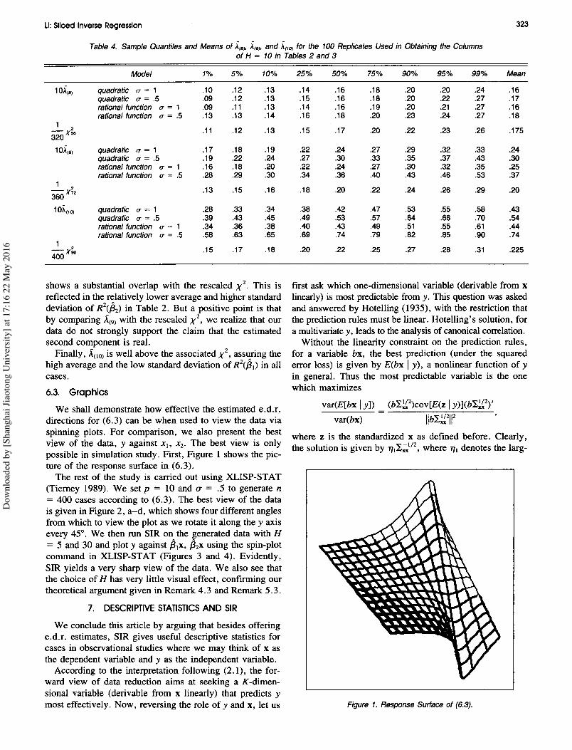
6.3. GraphicsWe shall demonstrate how effective the estimated e.d.r.

directions for (6.3) can be when used to view the data viaspinning plots. For comparison, we also present the bestview of the data, y against Xl, X2' The best view is onlypossible in simulation study. First, Figure 1 shows the pic-ture of the response surface in (6.3).The rest of the study is carried out using XLISP-STAT

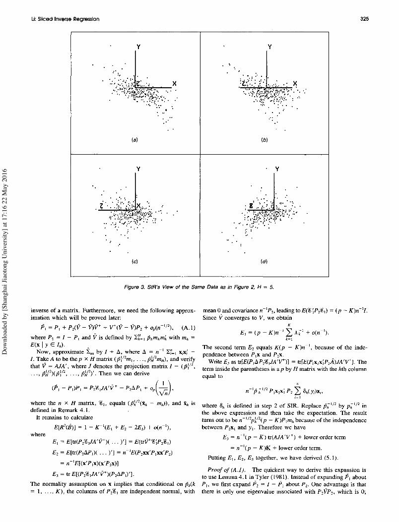
(Tierney 1989). We set p = 10 and (T = .5 to generate n= 400 cases according to (6.3). The best view of the datais given in Figure 2, a-d, which shows four different anglesfrom which to view the plot as we rotate it along the y axisevery 45°. We then run SIR on the generated data with H= 5 and 30 and plot y against {:JlX, {:J2X using the spin-plotcommand in XLISP-STAT (Figures 3 and 4). Evidently,SIR yields a very sharp view of the data. We also see thatthe choice of H has very little visual effect, confirming ourtheoretical argument given in Remark 4.3 and Remark 5.3.

We conclude this article by arguing that besides offeringe.d.r. estimates, SIR gives useful descriptive statistics forcases in observational studies where we may think of x asthe dependent variable and y as the independent variable.According to the interpretation following (2.1), the for-

ward view of data reduction aims at seeking a K-dimen-sional variable (derivable from x linearly) that predicts ymost effectively. Now, reversing the role of y and x, let us

Dow

nloa

ded

by [S

hang

hai J

iaot

ong

Uni

vers

ity] a

t 17:

16 2

2 M

ay 2

016

324

(a)

(c)

Journal of the American Statistical Association, June 1991

y

'.z r:· ,e:. '.. ..e. .)(... IIIto; ••01 ""0 •..' f

(b)

(d)

Figure 2. Best View of Data Generated From (6.3) With o: = .5, P = 10.

est eigenvector of cov[E(z Iy)]. This is what the first com-ponent of SIR, attempts to estimate.Generalizing the above argument, the projection direc-

tion yielding the variable that is most predictable from y,subject to being uncorrelated with the first most predictablevariable, is a direction estimated by Similar intepreta-tion extends to the otherSince the appearance of the first version of this article,

four related works have been written. Duan and Li (in press)studied SIR for the case where K = I in more detail. Theygeneralized the implementation of SIR by allowing a gen-eral weighting scheme for conducting the principal com-ponent analysis. Li (1989) examined SIR from a differentangle. A projection pursuit approach was taken there, basedon the notion of dependent variable transformation to pro-vide a projection index. It brought out a nice connectionwith other works related to transformations (e.g., corre-spondence analysis, ACE, and the dummy variable ap-proach to multivariate analysis by the Gill school) Li (1990a)proposed a new method for handling the case where theregression function may be symmetric. Li (1990b) appliedSIR to uncertainty analysis of mathematical models or com-puter models. SIR was used to visualize and simplify themodels.

APPENDIX

A.1. Proof of Theorem 3.1. Without loss of generality, as-sume that E(x) = O. Consider any vector b in the orthogonal com-plement of the space spanned by (3kI",,(k = 1, ... , K); that is,es;» = O.We need to show that bE(x Iy) = 0 with probability1. Equation (1.1) implies

bE(x Iy) = E[E(bx I (3kX' S, y) Iy] = E[E(bx I (3kX' S) Iy].Hence it suffices to show that E(bx I (3kX'S) = 0; or equivalently,E[(E(bx I {3kX'S))2] = O. By conditioning, the left term can bewritten as E[E(bx I (3kx's)x'b'], which equals E[(co +Ck{3kX)x'b'] = Ck{3kIxxb' = O. The proof of Therem 3.1 isnow complete.

A.2. Derivation of formula (5.1) for E[R 2(B )] . Due to theaffine invariance, we may assume that x has mean 0 and covari-ance I"" = 1. The squared trace correlation R2(B ) reduces to

K- I tr PIPI = 1 - K- 1 tr (PI - PI)PI(P I - PI),

where P I and PI are symmetric projection matrices associated withthe e.d.r. space B and the estimated space B respectively. Fromsteps 4 and 5 of SIR, PI is related to PI = T,icT,b a projectionmatrix:

P =1 l""-'xx 1 """xx ,

where the superscript + denotes the Moore-Penrose generalized

Dow

nloa

ded

by [S

hang

hai J

iaot

ong

Uni

vers

ity] a

t 17:

16 2

2 M

ay 2

016

Li: Sliced Inverse Regression

(a)

y

..=i..':.:::.: }: eo •• X

.:' ... ..

(b)

325

(e)

y

: I'>/}I;;::.::::,-.' .: :':p"':·f... '..' ..'

(d)

Figure 3. SIR's View of the Same Data as in Figure 2, H = 5.

inverse of a matrix. Furthermore, we need the following approx-imation which will be proved later:

P, = P, + PzCV - V)V+ + V+(V - V)Pz + oin-'/z), (A.l)

where Pz = I - PI and V is defined by PhmhmJ. with m; =E(x lyE I h ) .Now, approximate i"" by I + where = n-' Xjx!

I. Take A to be the p x H matrix (pJlzmh ... , pJ/zmH), and verifythat V = AlA', where J denotes the projection matrix I - (pllz,... , pJ/Z)(plIZ, ... , pJ/Z), . Then we can derive

, _+ ( 1 )(P, - P,)PI = Pz'f."JA'V - + op vn 'where the n x H matrix, 'f.,j, equals (Pkl\Xh - mh», and Xh isdefined in Remark 4.1.It remains to calculate

E[Rz(B)] = 1 - K-I(E1 + Ez - 2E3) + o(n- I),

whereE, = E[tr(Pz'f."JA'V+)( ... )'] = E(trV+'f.,;Pz'f.,,)

E 2 = E[tr(PzMI)( ... )'] = n-IE(Pzxx'Plxx'Pz)

= n-'E[(x'P,x)(x'Pzx)]

E 3 = tr E[(Pz'f.,IJA'V+)(PzMI)'].The normality assumption on x implies that conditional on Pk(k= 1, ... , K), the columns of PZ'f.,1 are independent normal, with

mean 0 and covariance n-Ipz, leading to E('f., ;PZ'f.,I) = (p - K)n-II.Since V converges to V, we obtain

K

E I = (p - K)n- I 2: A,;I + o(n- I).

The second term Ez equals K(p - K)n- I, because of the inde-pendence between PIX and Pzx.Write E3 as = tr[E(Pjx1x;PzA)JA'v+]. The

term inside the parentheses is a p by H matrix with the hth columnequal to

where 8h is defined in step 2 of SIR. Replace p;;'/Z by p;;'/Z inthe above expression and then take the expectation. The resultturns out to be n-'/Zpklz(P - K)Plmh because of the independencebetween PZXI and y,. Therefore we have

E 3 = n-'(p - K) tr(AJA'V+) + lower order term= n-I(p - K)K + lower order term.

Putting E h Ez, E3 together, we have derived (5.1).

Proof of (A.]). The quickest way to derive this expansion isto use Lemma 4.1 in Tyler (1981). Instead of expanding PI aboutPI' we first expand Pz = I - PI about P z. One advantage is thatthere is only one eigenvalue associated with PzVPz, which is 0;

Dow

nloa

ded

by [S

hang

hai J

iaot

ong

Uni

vers

ity] a

t 17:

16 2

2 M

ay 2

016

326

y

.-:: s: .::_::. e.. .• '. .::/1....: .;. •

.... -.,.

(a)

(e)

Journal of the American Statistical Association, June 1991

y

,..: .'. _.. X

(b)

(d)

Figure 4 (a)-(d). Best View of the Same Data as in Figure 2, H = 30.

so the Taylor expansion formula is simpler. This leads toP2 = P2 - [P2(Y - V)Y+ + Y+(Y - Y)P2] + op(n- 1/ 2) ,

implying (A. 1).

A.3. Asymptotic expansionjor A(p-K)' The following lemmais the key to our asymptotic expansion.

Lemma A.i. Consider the expansionT(w) = T + wT(l) + w2T(2) + 0(w2),

where T(w), T, r», T(2) are symmetric matrices. Suppose that Tis nonnegative definite with rankK. Then the average of the smallestp - K eigenvalues of T(w), A(w), has the expansion

1A(w) = -- [wA(I) + w2A(2) ] + o(w2),

p-Kwhere A(I) = tr T(I)IT, A(2) = tr[T(2)IT - T(I)T+T(l)I1], and IT is thesymmetric projection matrix of rank p - K such that ITT = TIT= O.This lemma is a simplified version of a result in the pertur-

bation theory for finite dimensional spaces (see chap. 2 of Kato1976, p. 79, eq. (2.33)). To use this lemma, obtain, after astraightforward asymptotic expansion, that

Y- V = + + ++ + + ++ + op(l/n),

where = I;,.I/2 - I. Thus we may substitute V for T, n- I /2 forw, Yfor T(w) , nl / 2 times the first bracketed term for r», n timesthe second bracketed term for T(2), and IT by P2.Straightforward computation leads to

wA(I) = tr T(l) P2P2 = tr P2T(l) P2 = 0,w2A(2) = tr

where Q = 1 - lA/rAJ, a projection matrix with trace H - K- 1. Based on a conditional probability argument similar to thatused in deriving E 1 in (A.2), we can show that n :follows a X 2 distribution with (p - K)(H - K - 1) degrees offreedom. This completes the proof. Note that the normality as-sumption on x is not necessary if the conditional covariance ofP2x given y E h does not depend on h because Xh is asymptoti-cally normal by the central limit theorem.

[Received July 1988. Revised March 1990.)

REFERENCES

Bickel, P. J., and Doksum, K. A. (1981), "An Analysis of Transfor-mations Revisited," Journal of the American Statistical Association.76, 296-311.

Breiman, L., and Friedman, J. (1985), "Estimating Optimal Transfor-mations for Multiple Regression and Correlation," Journal of theAmerican Statistical Association 80, 580-597.

Breiman, L., Friedman, J., Olshen, R., and Stone, C. (1984), Classi-fication and Regression Trees. Belmont, CA: Wadsworth.

Dow

nloa

ded

by [S

hang

hai J

iaot

ong

Uni

vers

ity] a

t 17:

16 2

2 M

ay 2

016

Li: Sliced Inverse Regression

Brillinger, D. R. (1977), "The Identification of a Particular NonlinearTime Series System," Biometrika, 64, 509-515.

Brillinger, D. R. (1983), "A Generalized Linear Model with 'Gaussian'Regressor Variables." In A Festschriftfor Erick L. Lehmann, Belmont,CA: Wadsworth, pp. 97-114.

Box, G., and Cox, D. R. (1964), "An Analysis of Transformations,"Journal of the Royal Statistical Society, Ser. B, 26, 211-252.

Box, G., and Draper, IV. (1987), Empirical Model-Building and Re-sponse Surfaces, New York: John Wiley.

Carr, D. B., Littlefield, R. J., Nicholson, W. L., and Littlefield, J. S.(1987), "Scatterplot Matrix Techniques for Large N," Journal of theAmerican Statistical Association, 82, 424-437.

Carroll, R., and Ruppert, D. (1984), "Power Transformations When Fit-ting Theoretical Models to Data," Journal of the American StatisticalAssociation, 79, 321-328.

Chen, H. (1988), "Convergence Rates for Parametric Components in aPartly Linear Model." The Annals of Statistics, 16, 136-146.--- (in press), "Rates of Convergence for Projection Pursuit Regres-sion," The Annals of Statistics.

Cleveland, W. S. (1987), "Research in Statistical Graphics," Journal ofthe American Statistical Association 82, 419-423.

Cuzik, J. (1987), "Semipararnetric Additive Regression," unpublishedmanuscript.

Diaconis, P., and Freedman, D. (1984), "Asyrnptotics of Graphical Pro-jection Pursuit," The Annals of Statistics, 12, 793-815.

Donoho, D., Johnstone, I., Rousseeuw, P., and Stahel, W. (1985), "Dis-cussion of On Projection Pursuit," The Annals of Statistics, 13 496-499.

Donoho, D., and Johnstone, 1. (1989), "Projection-Based Smoothing,and a Duality With Kernel Methods," The Annals ofStatistics 17, 58-106.

Duan, N., and Li, K. C. (in press), "Slicing Regression: a Link-FreeRegression Method," The Annals of Statistics.

Engle, R. F., Granger, C. W. 1., Rice, J., and Weiss, A. (1986), "Semi-parametric Estimates of the Relation Between Weather and ElectricitySales," Journal of the American Statistical Association, 81, 310-320.

Eubank, R. L. (1988), Spline Smoothing and Nonparametric Regression,New York: Marcel Dekker.

Fill, J. A., and Johnstone, 1. (1984), "On Projection Pursuit Measuresof Multivariate Location and Dispersion," The Annals ofStatistics, 12,127-141.

Friedman, J. (1987), "Exploratory Projection Pursuit," Journal of theAmerican Statistical Association, 82, 249-266.

Friedman, J., and Stuetzle, W. (1981), "Projection Pursuit Regression,"Journal of the American Statistical Association, 76, 817-823.

Hardie, W., Hall, P., and Marron, S. (1988), "How Far Are Automat-ically Chosen Regression Smoothing Parameters From Their Opti-mum," Journal of the American Statistical Association, 83, 86-101.

Hall, P. (1989), "On Projection Pursuit Regression," The Annals of Sta-tistics 17, 573-588.

Hastie, T., and Tibshirani, R. (1986), "Generalized Additive Models,"Statistical Science, 1, 297-318.

Heckman, N. (1986), "Spline Smoothing in Partly Linear Models," Jour-nal of the Royal Statistical Society Ser. B, 48, 244-248.

Hinkley, D. V., and Runger, G. (1984), "The Analysis of Transformed

327

Data," with discussion, Journal of the American Statistical Associa-tion, 79, 302-320.

Hooper, J. (1959), "Simultaneous Equations and Canonical CorrelationTheory," Econometrica, 27, 245-256.

Hotelling, H. (1935), "The Most Predictable Criterion," Journal of Ed-ucational Psychology, 139-142.

Huber, P. (1985), "Projection Pursuit," with discussion, The Annals ofStatistics, 13, 435-526.

Huber, P. (1987), "Experiences With Three-Dimensional Scatterplots,"Journal of the American Statistical Association, 82, 448-454.

Kato, T. (1976), Perturbation Theory for Linear Operators (2nd ed.),Berlin: Springer-Verlag.

Koyak, R. (1987), "On Measuring Internal Dependence in a Set of Ran-dom Variables," The Annals of Statistics, 15, 1215-1228.

Li, G., and Chen, Z. (1985), "Projection Pursuit Approach to RobustDispersion Matrices and Principal Components: Primary Theory andMonte Carlo." Journal of the American Statistical Association, 80, 759-766.

Li, K. C. (1987), "Asymptotic Optimality for c; C" Cross-Validationand Generalized Cross-Validation: Discrete Index Set," The Annals ofStatistics, 15, 958-975.--- (1989), "Data Visualization With SIR: a Transformation BasedProjection Pursuit Method," UCLA statistical series 24.--- (1990a), "On Principal Hessian Directions for Data Visualizationand Dimension Reduction: Another Application of Stein's Lemma,"UCLA technical report, Dept. of Mathematics.--- (1990b), "Uncertainty Analysis for Mathematical Models WithSIR," UCLA technical report, Dept. of Mathematics.

Li, K. C., and Duan, N. (1989), "Regression Analysis Under Link Vi-olation," The Annals of Statistics, 17, 1009-1052.

Loh, W. Y., and Vanichsetakul, N. (1988), "Tree-Structured Classifi-cation via Generalized Discriminant Analysis," Journal of the Amer-ican Statistical Association 83, 715-728.

Mallows, C. L. (1961), "Latent Vectors of Random Symmetric Matri-ces," Biometrika, 48,133-149.

Mardia, K. V., Kent, J. T., and Bibby, J. M. (1979), Multivariate Anal-ysis. New York: Academic Press.

Portnoy, S. (1985), "Asymptotic Behavior of M-Estimators of p Regres-sion Parameters When p'ln is Large II: Normal Approximation," TheAnnals of Statistics, 13, 1403-1417.

Speckman, P. (1987), "Kernel Smoothing in Partial Linear Models, " un-published manuscript.

Stone, C. (1986), "The Dimensionality Reduction Principle for Gener-alized Additive Models," The Annals of Statistics, 13, 689-705.

Tierney, L. (1989), "XLISP.STAT: A Statistical Environment Based onthe XLISP Language," (Beta Test Version 2.0). School of Statistics,University of Minnesota.

Tyler, D. (1981), "Asymptotic Inference for Eigenvectors," The Annalsof Statistics, 9, 725-736.

van Rijckevorsel, L. A., and de Leeuw, J. (1988), Component and Cor-respondence Analysis, New York: John Wiley.

Wahba, G. (1986), "Partial and Interaction Splines for SemiparametricEstimation of Functions of Several Variables," in Computer Scienceand Statistics: Proceedings of the 18-th Symposium on the Interface,Washington, D.C., pp. 75-80.D

ownl

oade

d by

[Sha

ngha

i Jia

oton

g U

nive

rsity

] at 1

7:16

22

May

201

6