slides for chapter 14: time and global states
TRANSCRIPT

From Coulouris, Dollimore, Kindberg and
Blair
Distributed Systems:
Concepts and Design
Edition 5, © Addison-Wesley 2012
Slides for Chapter 14:
Time and Global States

Overview of Chapter
• Introduction
• Clocks, events, process states
• Synchronizing physical clocks
• Logical time and logical clocks
• Global states (skip)
• Distributed debugging (skip)
2

Introduction
• Some applications need to record the time when events occur (e.g.
ecommerce, banking)
• May need to determine the relative order in which certain events
occurred
• Physical events order based on observer’s frame of reference
• Multiple computer clocks may be skewed and need to by
synchronized – no absolute global time for all computers in a
distributed systems
3

Overview of Chapter
• Introduction
• Clocks, events, process states
• Synchronizing physical clocks
• Logical time and logical clocks
• Global states
• Distributed debugging
4

Clocks, events, process states
• Each process can observe/cause multiple events
• Some events may change process states (data)
• History of a process: the series of events that take place within the
process ordered in a total ordering
Clocks:
• Each computer has a physical clock
• Timestamp: date/time that an event occurred
• Clock skew: instantaneous difference between two clocks
• Clock drift: different clocks count time at slightly different speeds
• UTC (Coordinated Universal Time): based on atomic time –
international standard for time keeping
5

Instructor’s Guide for Coulouris, Dollimore, Kindberg and Blair, Distributed Systems: Concepts and Design Edn. 5
© Pearson Education 2012
Figure 14.1
Skew between computer clocks in a distributed system
Overview of Chapter
• Introduction
• Clocks, events, process states
• Synchronizing physical clocks
• Logical time and logical clocks
• Global states
• Distributed debugging
7
Synchronizing physical clocks
External synchronization:
• Synchronizes each clock in the distributed system with a UTC
source – clocks must be within drift bound D of UTC
Internal synchronization:
• Synchronizes the clocks in the distributed system with one another –
any two physical clocks must be within drift bound D of one another
• May drift from UTC but are synchronized together
• Faulty clock: does not stay within specified drift bound
8
Synchronizing physical clocks
Synchronization in a synchronous system:
• Synchronous system has upper bound on message transmission
time max – also min is the minimum message transmission time
between two machines
• A message sent from node p at (local clock) time t arrives at another
node q at (local clock) time t’
• Can now set clock at node q to t + (max + min)/2 to synchronize
clock at node q with clock in node p
9
Synchronizing physical clocks using a time server node
NTP (Network Time Protocol):
• Synchronize clock at each node with clock at time server
• Assumes asynchronous system
Christian’s algorithm:
• Process p requests time from time server in message mr, receives
time value t in message mt
• P records round trip time Tround between sending and receiving
• P sets local clock time to t + Tround /2
• Probabilistic method
• All processes (nodes) synchronize with clock server node
• Used for synchronizing nodes on a local intranet
• Variation called Berkeley algorithm
10

Instructor’s Guide for Coulouris, Dollimore, Kindberg and Blair, Distributed Systems: Concepts and Design Edn. 5
© Pearson Education 2012
Figure 14.2
Clock synchronization using a time server
mr
m t
p Time server,S

Synchronizing physical clocks using NTP
NTP (Network Time Protocol):
• Synchronize clocks of client nodes on the internet with UTC
• Employs statistical techniques to factor in network latency
Other features:
• Can survive lengthy losses of connectivity
• Enables clients to synchronize frequently to offset drift
• Protects against interference with time services
Three modes of synchronization:
• Multicast mode (on a high speed LAN)
• Procedure call mode (similar to Christian’s algorithm)
• Symmetric mode (used by time servers)
12
Instructor’s Guide for Coulouris, Dollimore, Kindberg and Blair, Distributed Systems: Concepts and Design Edn. 5
© Pearson Education 2012
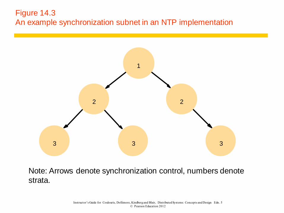
Figure 14.3
An example synchronization subnet in an NTP implementation
1
2
3
2
3 3
Note: Arrows denote synchronization control, numbers denote
strata.
Instructor’s Guide for Coulouris, Dollimore, Kindberg and Blair, Distributed Systems: Concepts and Design Edn. 5
© Pearson Education 2012
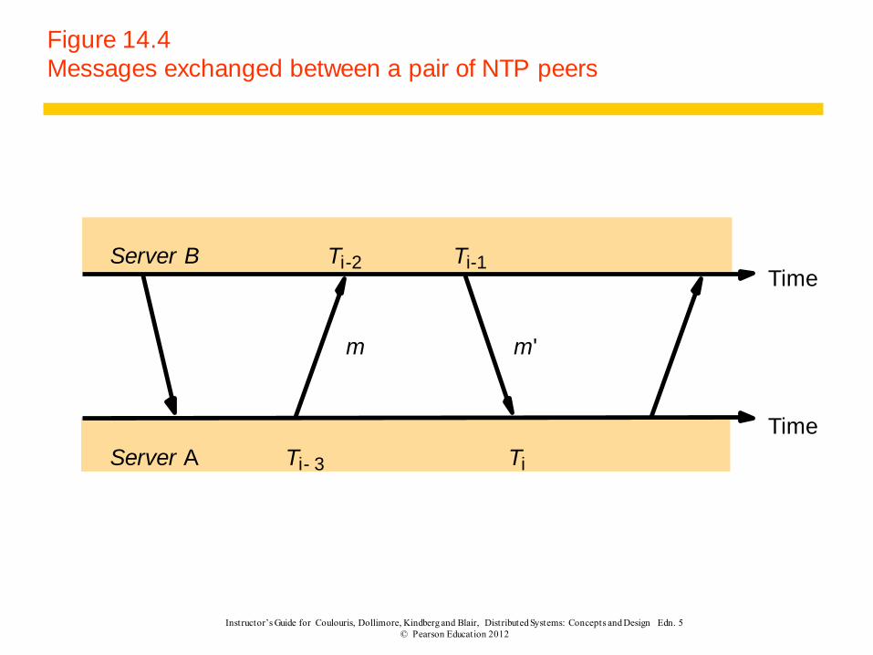
Figure 14.4
Messages exchanged between a pair of NTP peers
Ti
Ti-1Ti-2
Ti- 3
Server B
Server A
Time
m m'
Time

Overview of Chapter
• Introduction
• Clocks, events, process states
• Synchronizing physical clocks
• Logical time and logical clocks
• Global states
• Distributed debugging
15
Logical time and logical clocks
Ordering events that occur in different processes (nodes):
• Within each process pi events are ordered (->i)
• Sending a message from one process occurs before the message is
received at another process
Happened-before relationship -> based on above two observations:
• If e ->i e’, then e -> e’
• For any message m, send(m) -> receive(m)
• If e -> e’ and e’ -> e’’, then e -> e’’
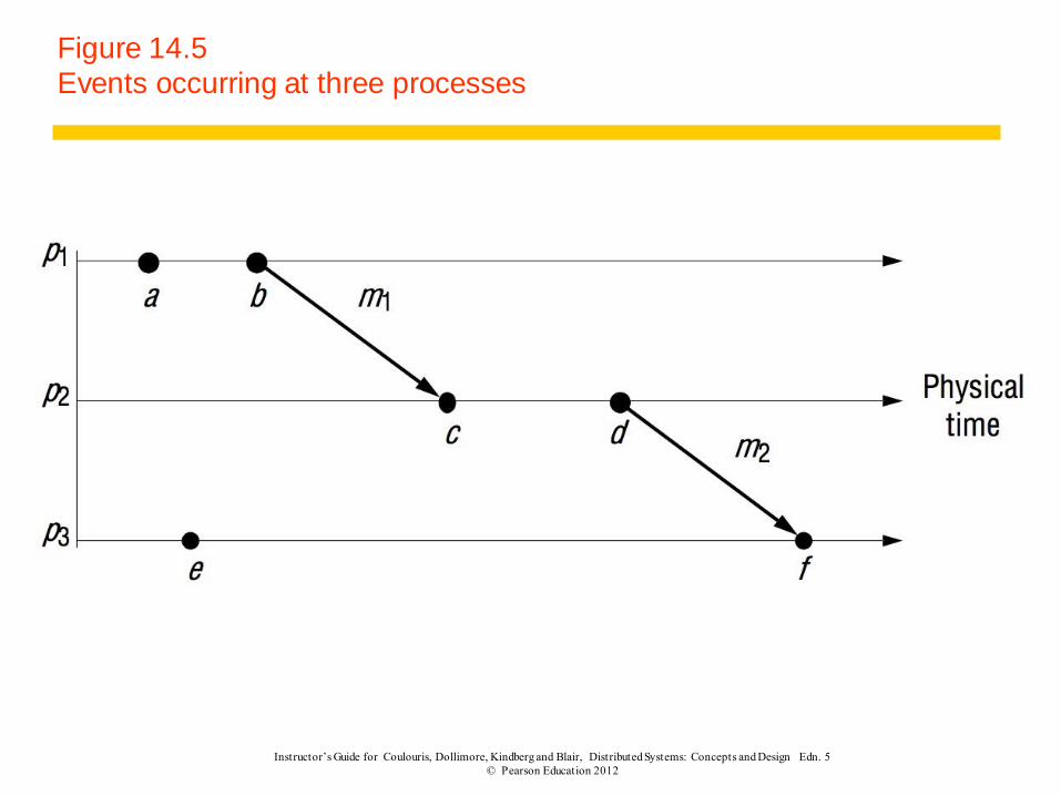
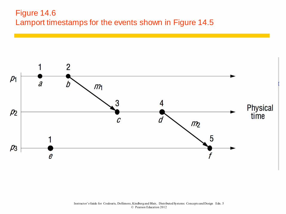
In next figure:
• a -> b, c -> d (same process); b -> c, d - > f (send/receive)
• a || e (concurrent; cannot tell which occurred first)
16
Instructor’s Guide for Coulouris, Dollimore, Kindberg and Blair, Distributed Systems: Concepts and Design Edn. 5
© Pearson Education 2012
Figure 14.5
Events occurring at three processes
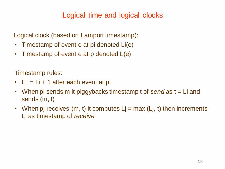
Logical time and logical clocks
Logical clock (based on Lamport timestamp):
• Timestamp of event e at pi denoted Li(e)
• Timestamp of event e at p denoted L(e)
Timestamp rules:
• Li := Li + 1 after each event at pi
• When pi sends m it piggybacks timestamp t of send as t = Li and
sends (m, t)
• When pj receives (m, t) it computes Lj = max (Lj, t) then increments
Lj as timestamp of receive
18
Instructor’s Guide for Coulouris, Dollimore, Kindberg and Blair, Distributed Systems: Concepts and Design Edn. 5
© Pearson Education 2012
Figure 14.6
Lamport timestamps for the events shown in Figure 14.5

Logical time and logical clocks
Totally ordered logical clock:
• Events can have same clock at two processes pi, pj
• By appending process id (t, i), a total order is achieved
• Order of processes not significant
Vector clocks:
• Keep a vector Vi[j], j = 1, 2, …, n of all time points of processes that
have communicated with pi
• Process vector always piggybacked with a sent message
• Receiving process can use piggybacked vector to update its vector
clock
20

Instructor’s Guide for Coulouris, Dollimore, Kindberg and Blair, Distributed Systems: Concepts and Design Edn. 5
© Pearson Education 2012
Figure 14.7
Vector timestamps for the events shown in Figure 14.5

Overview of Chapter
• Introduction
• Clocks, events, process states
• Synchronizing physical clocks
• Logical time and logical clocks
• Global states (skip)
• Distributed debugging
22

Instructor’s Guide for Coulouris, Dollimore, Kindberg and Blair, Distributed Systems: Concepts and Design Edn. 5
© Pearson Education 2012
Figure 14.8
Detecting global properties

Instructor’s Guide for Coulouris, Dollimore, Kindberg and Blair, Distributed Systems: Concepts and Design Edn. 5
© Pearson Education 2012
Figure 14.9
Cuts
m1 m2
p1
p2Physical
time
e1
0
Consistent cut
Inconsistent cut
e1
1e
1
2e
1
3
e 20
e 21
e 22
Instructor’s Guide for Coulouris, Dollimore, Kindberg and Blair, Distributed Systems: Concepts and Design Edn. 5
© Pearson Education 2012
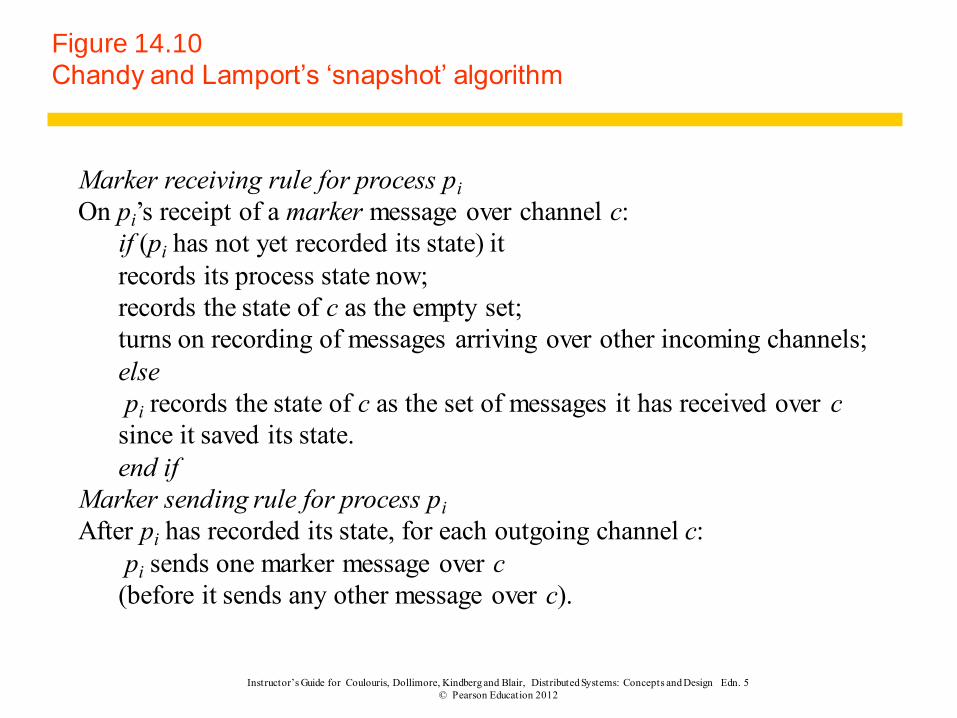
Figure 14.10
Chandy and Lamport’s ‘snapshot’ algorithm
Marker receiving rule for process pi
On pi’s receipt of a marker message over channel c:
if (pi has not yet recorded its state) it
records its process state now;
records the state of c as the empty set;
turns on recording of messages arriving over other incoming channels;
else
pi records the state of c as the set of messages it has received over c
since it saved its state.
end if
Marker sending rule for process pi
After pi has recorded its state, for each outgoing channel c:
pi sends one marker message over c
(before it sends any other message over c).

Instructor’s Guide for Coulouris, Dollimore, Kindberg and Blair, Distributed Systems: Concepts and Design Edn. 5
© Pearson Education 2012
Figure 14.11
Two processes and their initial states

Instructor’s Guide for Coulouris, Dollimore, Kindberg and Blair, Distributed Systems: Concepts and Design Edn. 5
© Pearson Education 2012
Figure 14.12
The execution of the processes in Figure 14.11
Instructor’s Guide for Coulouris, Dollimore, Kindberg and Blair, Distributed Systems: Concepts and Design Edn. 5
© Pearson Education 2012
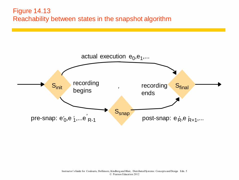
Figure 14.13
Reachability between states in the snapshot algorithm
Sinit Sfinal
Ssnap
actual execution e0,e1,...
recording recording begins ends
pre-snap: e'0,e '1,...e'R-1 post-snap: e 'R,e 'R+1,...
'

Overview of Chapter
• Introduction
• Clocks, events, process states
• Synchronizing physical clocks
• Logical time and logical clocks
• Global states
• Distributed debugging (skip)
29

Instructor’s Guide for Coulouris, Dollimore, Kindberg and Blair, Distributed Systems: Concepts and Design Edn. 5
© Pearson Education 2012
Figure 14.14
Vector timestamps and variable values for the execution of Figure 14.9
m1 m2
p1
p2Physical
time
Cut C1
(1,0) (2,0) (4,3)
(2,1) (2,2) (2,3)
(3,0)
x1= 1 x1= 100 x1= 105
x2= 100 x2= 95 x2= 90
x1= 90
Cut C 2
Instructor’s Guide for Coulouris, Dollimore, Kindberg and Blair, Distributed Systems: Concepts and Design Edn. 5
© Pearson Education 2012
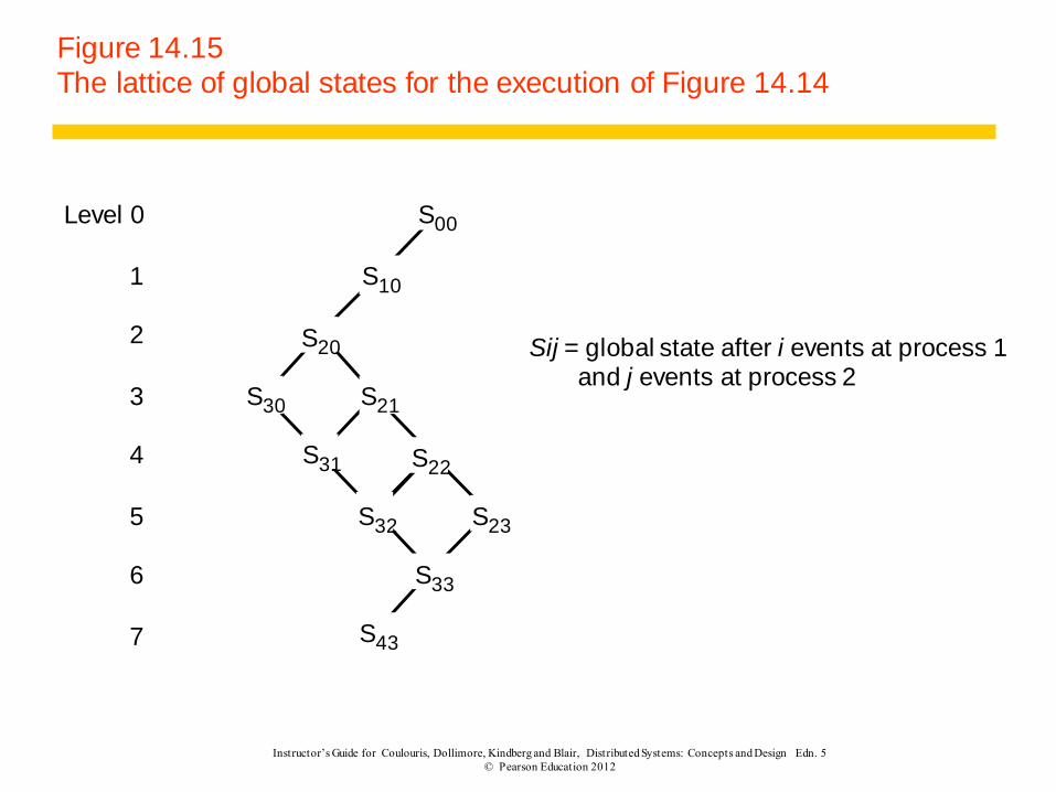
Figure 14.15
The lattice of global states for the execution of Figure 14.14
Sij = global state after i events at process 1and j events at process 2
S00
S10
S20
S21S30
S31
S32
S22
S23
S33
S43
Level 0
1
2
3
4
5
6
7

Instructor’s Guide for Coulouris, Dollimore, Kindberg and Blair, Distributed Systems: Concepts and Design Edn. 5
© Pearson Education 2012
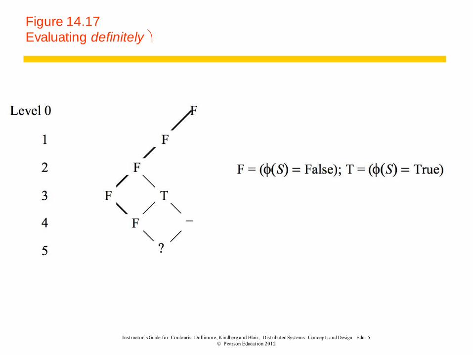
Figure 14.16
Algorithms to evaluate possibly and definitely
Instructor’s Guide for Coulouris, Dollimore, Kindberg and Blair, Distributed Systems: Concepts and Design Edn. 5
© Pearson Education 2012
Figure 14.17
Evaluating definitely