small- and waiting-time behaviour of the thin-film

SMALL- AND WAITING-TIME BEHAVIOUR OF THE THIN-FILMEQUATION.

READING UNIVERSITY NUMERICAL ANALYSIS REPORT 9/06

JAMES F. BLOWEY∗§ , JOHN R. KING† , AND STEPHEN LANGDON‡§¶

Abstract. We consider the small-time behaviour of interfaces of zero contact angle solutions tothe thin-film equation. For a certain class of initial data, through asymptotic analyses, we deduce awide variety of behaviour for the free boundary point. These are supported by extensive numericalsimulations.

Key words. thin-film, waiting-time, interface, nonlinear degenerate parabolic

AMS subject classifications. 35R35, 35K35, 35K55, 35K65, 65M60

1. Introduction. This paper is concerned with the small-time behaviour of in-terfaces of zero contact angle solutions to the “thin-film” equation

∂h

∂t= − ∂

∂x

(hn ∂3h

∂x3

), (1.1a)

with h = h0(x) at t = 0 and (1.1b)

h =∂h

∂x= hn ∂3h

∂x3= 0 at x = s(t), (1.1c)

where h ≥ 0 represents the thickness of a fluid film and x = s(t) denotes the right-handinterface (with h ≡ 0 for x > s(t)); since we are concerned with the local behaviour atsuch an interface we need not specify conditions at any left-hand moving boundary.The first boundary condition of (1.1c) defines the moving boundary (as the point atwhich the film thickness reaches zero), the second ensures a zero contact angle, andthe third represents conservation of mass.

In the last few years the range 0 < n ≤ 3 has been considered in the literature froma modelling point of view. With n = 3, (1.1a–c) models the lubrication approximationof a surface tension driven thin viscous film spreading on a solid horizontal surface,with a no-slip condition at the solid/liquid/air interface [5, 6, 10, 11, 12, 14, 30].However, the no-slip condition implies an infinite force at the interface [18, 24]. Toavoid this, more realistic models allowing slip have been proposed (see e.g. [4, 19, 23])for which it has been shown that the qualitative behaviour of solutions in the vicinityof the interface corresponds to that of the solution of (1.1a–c) with n ∈ (0, 3); thisapplies to questions of spreading or non-spreading as well as to questions of locallypreserved positivity and local film rupture [16]. With n ∈ (0, 3) it is also well known(see e.g. [7, 8]) that (1.1a–c) admits solutions with a finite speed of propagationproperty, i.e. s(t) represents a moving boundary, which moves at finite speed.

In this paper we thus consider only values of n in the moving front regime 0 <n < 3, and we assume further that the film is thick enough that Van der Waals forces

∗Department of Mathematical Sciences, University of Durham, DH1 3LE, U.K.([email protected]).

†School of Mathematical Sciences, University of Nottingham, University Park, Nottingham, NG72RD, U.K. ([email protected]).

‡Department of Mathematics, University of Reading, Whiteknights, PO Box 220, Berkshire RG66AX, U.K. ([email protected]).

§Partially supported by the EPSRC, U.K. through grant GR/M30951.¶Partially supported by a Leverhulme Trust Early Career Fellowship.

1

2 J.F.BLOWEY, J.R.KING AND S.LANGDON

play no part. When considering solutions to (1.1a–c), the primary physical question isoften to do with the movement of the free boundary. Where h = 0 there is no diffusionin (1.1a), and this can lead to waiting-time behaviour, where the interface remainsstationary for a period before moving; alternatively the interface may either advanceor retreat immediately. A determination of the regimes in which such behaviour canoccur has considerable implications regarding the possibility of film rupture in thepresence of a very thin pre-wetting layer; see e.g. [27].

There has been much recent effort in the literature to answer outstanding ques-tions about the initial movement of the interface. Theoretical results in [4, 5] haveshown that the interface cannot retreat if n ≥ 3/2, but that film rupture may occurfor n < 1/2 (see also [13, 14]). Moreover, numerical evidence [4, 10, 12] suggests thatfor small values of n solutions which are initially strictly positive may vanish at somepoint x0 after a finite time t0, with the solution becoming zero on a set of positivemeasure shortly after the finite time singularity, a phenomenon called “dead core” inother fields. The existence of a critical exponent (a value of n∗ > 0 for which solutionsstay positive for n > n∗ and where finite-time singularities are possible for n ≤ n∗)has been conjectured in [11], where it is remarked that numerical simulations suggest1 < n∗ < 3.5. Our results below support and clarify these conjectures; in particular,here we provide the first concrete solutions to (1.1a–c) displaying retreat.

As explained in [27], subsequent to any waiting time the local behaviour of solu-tions to (1.1a–c) takes the form

h ∼(

n3s

3(3 − n)(2n − 3)(s − x)3

) 1n

as x → s−, for 32 < n < 3, (1.2)

h ∼(

3

4s(s − x)3 ln [1/(s − x)]

) 23

as x → s−, for n = 32 , (1.3)

h ∼ B(t)(s − x)2 as x → s−, for n < 32 . (1.4)

With 0 < n < 3, in (1.2) we require that s > 0, whereas in (1.4) the interface velocitys may take either sign, with B(t) determined as part of the solution. One of the keymotivations for the current analysis is to provide criteria under which s < 0 holdsfor sufficiently small time; since s > 0 typically holds for large times, for example forthe Cauchy problem with initial data of finite mass, a large-time analysis provides noinsight into such matters.

For definiteness, we shall consider the case

h0(x) ∼ A0(x0 − x)α + C0(x0 − x)β as x → x−

0 (1.5)

where A0, α and β are positive constants with β > α, C0 is a constant and x0 = s(0).Extensive studies of the small-time behaviour have already been done for the

corresponding second-order problem, the porous-medium equation.

∂h

∂t=

∂

∂x

(hn ∂h

∂x

)(1.6)

with n > 0. We present our results in this context. The variety of possible small-time behaviours for (1.1a–c) is summarised in Figure 1.1, and can be characterised asfollows;

(i) For α greater than some critical value, the interface “waits” for some finite timetw, whereby

s(t) = x0 for 0 ≤ t ≤ tw,

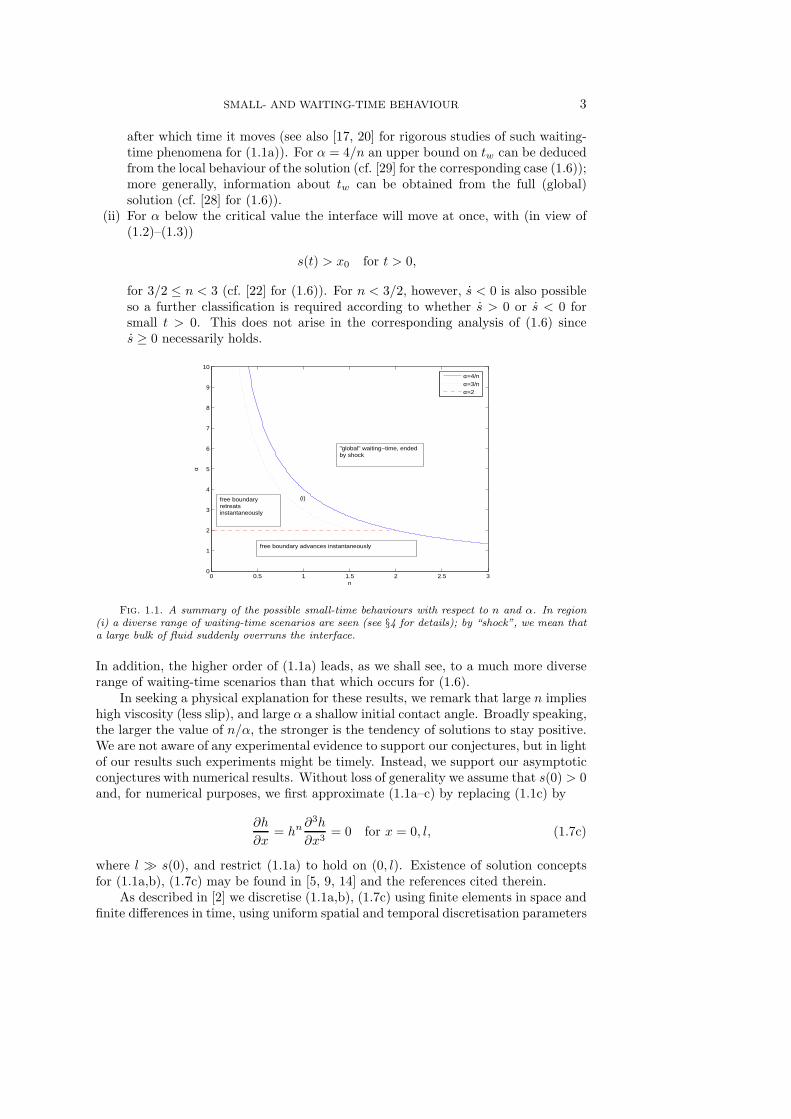
SMALL- AND WAITING-TIME BEHAVIOUR 3

after which time it moves (see also [17, 20] for rigorous studies of such waiting-time phenomena for (1.1a)). For α = 4/n an upper bound on tw can be deducedfrom the local behaviour of the solution (cf. [29] for the corresponding case (1.6));more generally, information about tw can be obtained from the full (global)solution (cf. [28] for (1.6)).

(ii) For α below the critical value the interface will move at once, with (in view of(1.2)–(1.3))

s(t) > x0 for t > 0,

for 3/2 ≤ n < 3 (cf. [22] for (1.6)). For n < 3/2, however, s < 0 is also possibleso a further classification is required according to whether s > 0 or s < 0 forsmall t > 0. This does not arise in the corresponding analysis of (1.6) sinces ≥ 0 necessarily holds.

0 0.5 1 1.5 2 2.5 30

1

2

3

4

5

6

7

8

9

10

n

α

α=4/nα=3/nα=2

free boundary advances instantaneously

free boundaryretreatsinstantaneously

"global" waiting−time, endedby shock

(i)

Fig. 1.1. A summary of the possible small-time behaviours with respect to n and α. In region(i) a diverse range of waiting-time scenarios are seen (see §4 for details); by “shock”, we mean thata large bulk of fluid suddenly overruns the interface.

In addition, the higher order of (1.1a) leads, as we shall see, to a much more diverserange of waiting-time scenarios than that which occurs for (1.6).

In seeking a physical explanation for these results, we remark that large n implieshigh viscosity (less slip), and large α a shallow initial contact angle. Broadly speaking,the larger the value of n/α, the stronger is the tendency of solutions to stay positive.We are not aware of any experimental evidence to support our conjectures, but in lightof our results such experiments might be timely. Instead, we support our asymptoticconjectures with numerical results. Without loss of generality we assume that s(0) > 0and, for numerical purposes, we first approximate (1.1a–c) by replacing (1.1c) by

∂h

∂x= hn ∂3h

∂x3= 0 for x = 0, l, (1.7c)

where l ≫ s(0), and restrict (1.1a) to hold on (0, l). Existence of solution conceptsfor (1.1a,b), (1.7c) may be found in [5, 9, 14] and the references cited therein.

As described in [2] we discretise (1.1a,b), (1.7c) using finite elements in space andfinite differences in time, using uniform spatial and temporal discretisation parameters


δx and δt, respectively; see §2 for details. We expect this method to be able to computethe zero contact angle solution for the following reasons:

1. In [5], the existence of solutions to (1.1a,b), (1.7c) is proved for 0 < n < 3,where h(·, t) may be C1([0, l]) for almost every t > 0 (the zero contact anglesolution), or alternatively h(·, t) may have non-expansive support.

2. In [2] it was proved that the numerical solution converges, as δx, δt → 0,to a weak solution of (1.1a,b), (1.7c) (in the sense of [5, 9, 14]). The onlyremaining question is whether this is the zero contact angle solution, or asolution with non-expansive support.

3. In a sequence of experiments, taking δt = O(δx12 ), the numerical method

computes a solution with non-expansive support.4. In a sequence of experiments, taking δt = O(δx2), the numerical method can

compute solutions where |s(0)| = ∞ (zero contact angle solutions).5. In [2] a self-similar source type solution was successfully computed with δt =

O(δx2). Moreover, taking a non-smooth stationary solution as initial data,i.e. h0(x) = α maxγ2−x2, 0 and 0 < γ < l, the numerical method computeda smooth solution for 0 < n < 3 and it was concluded that h(x, t) ≡ h0(x)for n > 3.

Hence in our experiments, in order to be sure that we are approximating the zerocontact angle solution we always choose δt = O(δx2). We report that the numericalsolution always appeared to be smooth.

An outline of the paper is as follows. We begin in §2 by describing our numericalscheme in more detail. We then proceed in §3 and §4 with a formal asymptoticanalysis, supported by numerical experiments, for the two cases α ≥ 4/n and α <4/n, respectively. Videos demonstrating more graphically how some of the numericalsolutions of these sections evolve over time can be found online athttp://www.personal.rdg.ac.uk/∼sms03sl/4thorder/4thorder.htmlFinally in §5 we present some conclusions.

2. Numerical Approximation. Following the approach of [2], and as describedin §1, we restrict (1.1a) to a finite space interval (0, l), introduce a potential w andrewrite it as the system of equations

∂h

∂t=

∂

∂x

(hn ∂w

∂x

)in (0, l) × (0, T ), (2.1a)

− ∂2h

∂x2= w in (0, l) × (0, T ). (2.1b)

A nonnegativity constraint is imposed on (2.1b) via a variational inequality in theweak form and then we discretise (2.1a,b) using the finite element method. Now givenpositive integers N and M , denote by δt := T/M and δx := l/N the temporal andspatial discretisation parameters, tk := kδt, k = 1, . . . , M , and xj = jδx, j = 0, . . . , N ,then the discretisation may be written in the following way.For k = 1, . . . , M and j = 1, . . . , N − 1 find Hk+1

j , W k+1j such that

Hk+1j − Hk

j

δt+

1

δx2

[∫ xj

xj−1

((x−xj−1)

δx Hkj +

(xj−x)δx Hk

j−1

)n

dx

](W k+1

j − W k+1j−1

δx

)

+1

δx2

[∫ xj+1

xj

((x−xj)

δx Hkj+1 +

(xj+1−x)δx Hk

j

)n

dx

](W k+1

j − W k+1j+1

δx

)= 0 (2.2a)


[−Hk+1

j+1 + 2Hk+1j − Hk+1

j−1

δx2− W k+1

j

]Hk+1

j = 0 (2.2b)

−Hk+1j+1 + 2Hk+1

j − Hk+1j−1

δx2− W k+1

j ≥ 0 (2.2c)

Hk+1j ≥ 0 (2.2d)

where Hkj ≈ h(xj , tk), W k

j ≈ w(xj , tk), H0j = h0(xj); similar equations/inequalities

appropriate for boundary data (1.7c) hold for j = 0, N when k = 1, . . . , M . This non-linear system is solved using a Gauss-Seidel algorithm in multigrid mode; for detailswe refer to [3]. We found this approach to have several advantages over some otheralgorithms previously proposed in the literature, such as the Uzawa type algorithm[2, (3.7a–c)], [21]. Specifically:

1. If Hkj−1 = Hk

j = Hkj+1 = 0 then it follows from (2.2a) that Hk+1

j = Hkj = 0,

so that the free boundary advances at most one mesh point from time level kto time level k + 1. The advantage of using the non-symmetric Gauss-Seidelsmoother is that this constraint is easier to impose on the numerical methodthan with a symmetric smoother.

2. Working within a multigrid framework significantly increases the rate of con-vergence. This allows us to reduce the tolerance for the stopping criterion ofthe iterative scheme (the maximum absolute difference in successive iteratesis smaller than tol) to tol = 10−12, as compared with tol = 10−8 in [2], andtherefore to solve the nonlinear system more accurately, thereby helping toavoid spurious behaviour.

3. Non-negativity of the computed numerical solution is guaranteed, so definingthe position xk

c of the numerical free boundary at time tk to be

xkc := xj > 0 : Hk

m ≤ ǫ for all m ≥ j, Hkj−1 > ǫ

we take ǫ = 0 which tracks the free boundary more accurately than withǫ > 0, this compares with ǫ = 10−6 in [2]. We remark that because thenumerical free boundary is defined on a discrete set of points, its movementappears to “stutter” in the figures below.

In the numerical experiments of §3 and §4 we solve (1.1a,b), (1.7c) with l = 1 and

h0(x) = 5 max(

916 − x2

)α, 0

; (2.3)

the key properties are that the maximum value of h0 is O(1) and the thin-film issymmetrically distributed about 0 with x0 = 3/4. These experiments were performedfor a sequence of space steps δx where δt = Cα,nδx2 and convergence of (2.2a)–(2.2d)to a weak solution of (1.1a,b), (1.7c), (2.3) was assured (see [2]). For reasons of spacewe refer to [15] for further figures and numerical results, including results from manymore experiments with values of n and α closer to the edges of the parameter regimes.

3. Formal asymptotic analysis and numerical results for α ≥ 4/n. Forα ≥ 4/n, the formal asymptotic analysis of this section suggests that we might expectwaiting-time behaviour. In particular, for α > 4/n (§3.1) we anticipate “global”waiting-time behaviour, by which we mean that the asymptotic expansion tells usto expect a waiting-time, but gives no clue as to the local behaviour; in this casethe interface starts to move due to “shock” formation, with the gradient becoming


unbounded near the free boundary. For α = 4/n (§3.2) this global breakdown canoccur for the full range 0 < n < 3, but for 2 < n < 3 “local” waiting-time behaviouris also possible; by this we mean that the dominant term in the asymptotic expansionswitches at the end of the waiting-time.

3.1. α > 4/n: “global” waiting-time behaviour. Provided h0(x) is analyticaway from the interfaces, then the small-time expansion

h ∼ h0 −d

dx

(h3

0

d3h0

dx3

)t as t → 0+ (3.1)

holds, at least away from the interface. From (1.5) we have

d

dx

(hn

0

d3h0

dx3

)∼ α(α − 1)(α − 2)((n + 1)α − 3)An+1

0 (x0 − x)(n+1)α−4

+ (nα(α − 1)(α − 2) + β(β − 1)(β − 2)) (nα + β − 3)An0 C0(x0 − x)nα+β−4

as x → x−

0 ; (3.2)

for α > 4/n we have (n + 1)α − 4 > α, and we may expect the local behaviour

h ∼ A0(x0 − x)α as x → x−

0 (3.3)

to hold up to some finite time t = tw > 0, implying a waiting-time scenario in whichthe local behaviour at the interface does not change for some non-zero waiting-time.

To test this conjecture, we ran numerical experiments for a large range of n andα > 4/n, considering in particular n = 0.75, 1.0, 1.75 and 2.5, so as to cover all of thedifferent regimes important in the case α < 4/n (see §4).

In the upper left plot of Figure 3.1 we plot xkc against tk for n = 1.75 and

α = 3.0 > 4/n = 2.29. The numerical free boundary remains stationary for a periodbefore advancing. We also plot profiles of Hk

j in the vicinity of the interface at times

just before and just after xkc begins to move (lower left plot). Shock-type behaviour

at the end of the waiting-time can be observed (cf. [28] for the second-order case).

0 0.001 0.002 0.003 0.004 0.005 0.006 0.007 0.008 0.009 0.01

0.75

0.76

0.77

0.78

0.746 0.7465 0.747 0.7475 0.748 0.7485 0.749 0.7495 0.75 0.7505 0.7510

0.2

0.4

0.6

0.8

1x 10

−6

tk=0

tk=7.25×10−3

tk=7.5×10−3

tk=7.75×10−3

tk

xk c

n = 1.75, α = 3.0

xj

Hk j

1 2 3 4 5 6 7 80

0.002

0.004

0.006

0.008

0.01

0.012

0.014

0.016

α

wa

itin

g tim

e

n=0.75n=1.0n=1.75n=2.5

Fig. 3.1. Waiting-time behaviour, various n, α.

Similar waiting-time behaviour, with shock type behaviour at the end of thewaiting-time, was observed for all n, α combinations tested in this range. Ap-proximate waiting times are plotted against α in the right half of Figure 3.1, for


n = 0.75, 1.0, 1.75, 2.5 and for various α > 4/n. For fixed n, the waiting time in-creases as α increases.

3.2. α = 4/n: “local” waiting-time behaviour for 2 < n < 3. In the criticalcase, the leading term in (1.5) suggests the separable local behaviour

h ∼ Λ(t)(x0 − x)4/n as x → x−

0 , (3.4)

with (1.1a–c) implying

Λ = − 4n

(4n − 1

) (4n − 2

) (4n + 1

)Λn+1.

Hence if n 6= 2 (recalling that we consider in this paper only 0 < n < 3),

Λ = A0

(1 +

8(4 − n)(2 − n)(n + 4)An0 t

n3

)−

1n

. (3.5)

This local solution also represents waiting-time behaviour; (3.5) blows up in finitetime if 2 < n < 3, so the waiting-time tw then satisfies

tw ≤ tc ≡ n3

8(4 − n)(n − 2)(n + 4)An0

;

Λ(t) decreases with time for 0 < n < 2, but we nevertheless expect (3.4) to remainvalid only up to some finite tw, after which the front begins to move due to shock,as described in §3.1. Thus for 2 < n < 3 local waiting-time behaviour (tw = tc)is possible, analogous to that for the porous-medium equation ([29]), while globalbreakdown (tw < tc for 2 < n < 3) can occur for the full range 0 < n < 3 (cf. [28]).

4. Formal asymptotic analysis and numerical results for α < 4/n. Webegin in §4.1 by deriving some local similarity solutions. Based on these and thelocal behaviour indicated in (1.2)–(1.4), we conjecture in §4.2–§4.6 some parameterregimes for the small-time behaviour when α < 4/n, in which case (3.3) fails for anyt > 0. This does not mean that for α < 4/n there is no waiting-time behaviour;on the contrary, unlike for the corresponding second-order problem (1.6), a diverserange of waiting-time scenarios can occur in this case. In addition to these waiting-time scenarios, the front may also advance or retreat instantaneously. Many of ourconjectures are supported by extensive numerical verifications, detailed below; weleave open their rigorous confirmation.

4.1. Local similarity solutions. In view of (1.5), a natural conjecture for thesmall-time behaviour for α < 4/n (balancing the terms in the expansion so they areof the same size) is the self-similar form

h ∼ tα

4−nα f((x − x0)/t

14−nα

), s(t) ∼ x0 + η0t

14−nα , (4.1)

where with η := (x − x0)/t1/(4−nα), f(η) satisfies the boundary-value problem

1

4 − nα

(αf − η

df

dη

)= − d

dη

(fn d3f

dη3

), (4.2)

as η → −∞ f ∼A0(−η)α−α(α−1)(α−2)((n + 1)α−3)An+10 (−η)(n+1)α−4, (4.3a)

at η = η0 f =df

dη= fn d3f

dη3= 0. (4.3b)


Here s(t) is the position of the contact line at time t, and η0 is a free constantdetermined by the boundary-value problem.

The behaviour as η → −∞ in (4.3a) thereby matches via (3.1) with the leadingterms in (1.5) and (3.2). The constant A0 can be scaled out by setting

f = A4

4−nα

0 f , η = An

4−nα

0 η,

suggesting in particular the delicacy of the limit α → (4/n)−, and the transformation

f = |η| 4n g(ξ), ξ = ln |η|

enables (4.2) to be reduced to a fourth-order autonomous problem. Nevertheless, thecomplexities of the resulting four-dimensional phase space mean that a global analysisof (4.2) (akin to that in [29] for the second-order problem) is not practicable here.Instead we base our conjectures in large part on a number of closed-form solutionsto (4.2) which we now note. We assume (4.2)–(4.3a,b) to have a unique non-negativesolution.

(I) Separable solution

f(η) =

(n3

8(4 − n)(2 − n)(n + 4)(−η)4

) 1n

(4.4)

is an explicit solution to (4.2) for 0 < n < 2, providing a possible localbehaviour as η → 0− for solutions with η0 = 0; the circumstances underwhich (4.4) may be applicable are clarified in Appendix A.

(II) Steady state solution

f(η) = A0(−η)2, η0 = 0, (4.5)

gives the solution to (4.2)–(4.3a,b) when α = 2.(III) Travelling wave solution

f(η) = A0(η0 − η)3n , η0 =

3(3 − n)(2n − 3)An0

n3, (4.6)

is the solution to (4.2)–(4.3a,b) when α = 3/n, n 6= 3/2; here η0 > 0 if3/2 < n < 3 and η0 < 0 if 0 < n < 3/2.

To complete our catalogue of pertinent closed form solutions we note that for n = 1the polynomial solution (cf. [25])

h =A3

0

4(1 + 30C20t/A0)C2

0

((1 + C0(x0 − x)/A0)

2 − (1 + 30C20t/A0)

25

)2

,

s = x0 − A0

((1 + 30C2

0 t/A0)15 − 1

)/C0, (4.7)

corresponds to

h0 = A0(x0 − x)2 + C0(x0 − x)3 + C20 (x0 − x)4/(4A0) (4.8)

so that α = 2, β = 3 in (1.5); hence s initially decreases if C0 > 0 but increases ifC0 < 0, with

s(t) ∼ x0 − 15C0t as t → 0+, (4.9)

this dependence on the sign of C0 being perhaps counter-intuitive, which is far fromunusual in such high-order diffusion problems.


4.2. Small-time behaviour for 2 < n < 3. In this regime, the solution (4.4)is not available to describe the local behaviour of f(η) at the interface; (4.6) hasthe expected local behaviour (1.2), while (4.5) corresponds to α > 4/n and thereforelies in the waiting-time regime discussed in §3.1. We thus anticipate that for anyα < 4/n the support of h expands immediately according to (4.1) with η0 > 0 and,in (4.2)–(4.3a,b),

f(η) ∼(

n3η0

3(3 − n)(2n − 3)(4 − nα)(η0 − η)3

) 1n

as η → η−

0 , (4.10)

which follows from (1.2). The interface advances with unbounded initial velocity forα < 3/n, with finite positive initial velocity if α = 3/n (with f(η) given by (4.6)) andwith velocity tending to zero as t → 0+ for α > 3/n. The behaviour in this regime isvery much analogous to that exhibited by the porous-medium equation (cf. [22]).

To test this conjecture we ran numerical experiments for n = 2.5, for which3/n = 1.2 and 4/n = 1.6, and for α ∈ [0.5, 1.5]. Our results support the conjecture.In each case xk

c advances, with the speed of the advance decreasing as α increases from0.5 to 1.5. We plot xk

c against tk for n = 2.5 and for α = 0.5 < 3/n and α = 1.4 > 3/nin the upper half of Figure 4.1. Note the different time scales on the two plots.

0 0.1 0.2 0.3 0.4 0.5 0.6 0.7 0.8 0.9 1

x 10−8

0.75

0.7505

0.751

0.7515

0.752

0.7525

0.753

−30 −28 −26 −24 −22 −20 −18−10

−9

−8

−7

−6

−5

tk

xk c

n = 2.5, α = 0.5

log tk

log(x

k c−

x0 c)

0 0.1 0.2 0.3 0.4 0.5 0.6 0.7 0.8 0.9 1

x 10−3

0.75

0.755

0.76

0.765

0.77

−16 −15 −14 −13 −12 −11 −10 −9 −8 −7−12

−10

−8

−6

−4

tk

xk c

n = 2.5, α = 1.4

log tk

log(x

k c−

x0 c)

Fig. 4.1. Numerical results for n = 2.5, α = 0.5, T = 10−8 (left), and for n = 2.5, α = 1.4,T = 10−3 (right). In the upper half of the figure the advancing free boundary is shown. In the lowerhalf of the figure log tk is plotted against log(xk

c − x0c) as a discrete set of points, with the solid line

following from a least squares fitting, the straight dotted line from asymptotic theory, and the dashedline in the lower right section following from a least squares fitting with the early data removed.

In the lower half of Figure 4.1 we test the hypothesis that for small times

xkc = x0

c + Atγk , (4.11)

for some constants A > 0 and γ, by plotting log(xkc − x0

c) against log tk (as a discreteset of points - these appear to “stutter” since the numerical free boundary advances byone discrete mesh point at a time). If the hypothesis is correct we expect a straight linewith slope γ. To estimate the value of γ we take a least squares fit. For presentationalpurposes we plot the best fitting least squares line as a solid line, and for comparisonwe also plot a dotted line with slope (4−nα)−1, the expected value of γ (recall (4.1)).


For α = 0.5 the log-log plot is fairly straight, and the estimated value of γ = 0.31is close to the expected value of 0.36. For α = 1.4 the best fitting least squares linegives an estimate of γ = 1.27, which is not close to the expected value of 2.00, and is apoor fit to the data. In this case the immediate yet slow advance of the free boundarymeans that for tk small, xk

c overestimates the exact position of the free boundary.This is demonstrated by the fact that the lowest horizontal line of dots on the log-logplot, corresponding to the first step in the advance of xk

c , matches very poorly withthe rest of the data. In the lower right plot of Figure 4.1 we thus also show as adashed line the best fitting least squares approximation to the data with the first stepin the advance of xk

c excluded (equivalently taking tk ' 5 × 10−5 rather than tk > 0on the log-log plot). This dashed line, with a slope of 1.69, matches the slope of thedata and the expected value of γ much more closely than our original estimate.

The expected and estimated values of γ for each value of α tested are shown inTable 4.1. For α ≤ 1.3 we estimate γ using all of the data, but for α = 1.4 andα = 1.5 we exclude the first step in the advance of xk

c , as discussed above. Thenumerical results give a value of γ slightly lower than the expected value, but thedifference is small, and the trend of γ increasing with α is clear. Our estimate for γis more accurate for values of α away from the edges of the parameter regime.

α 0.5 0.6 0.7 0.8 0.9 1.0 1.1 1.2 1.3 1.4 1.51

4−nα 0.36 0.40 0.44 0.50 0.57 0.67 0.80 1.00 1.33 2.00 4.00

γ 0.31 0.35 0.39 0.46 0.53 0.61 0.76 0.91 1.12 1.69 3.43Table 4.1

Estimated and expected values of γ for n = 2.5, various α.

4.3. Small-time behaviour for n = 2. The behaviour for α < 2 is as describedin §4.2. However, for α = 2 the solution (4.1) is not applicable and, partly becauseα = 2 will also play an important role in what follows, additional comments regardingthe resulting waiting-time scenario are instructive. The small-time solution (4.5)suggests that there is initially no change in local behaviour, while (3.2) becomes

d

dx

(hn

0

d3h0

dx3

)∼ (β + 1)β(β − 1)(β − 2)A2

0C0(x0 − x)βt; (4.12)

both suggest seeking a local solution of the form

h ∼ A0(x0 − x)2 + H(x, t) as x → x−

0 ; (4.13)

we note that H need not be positive on x < x0 because it represents a correction termto the (quadratic) leading order behaviour. Linearising in H yields

∂H

∂t= −A2

0

∂

∂x

((x0 − x)4

∂3H

∂x3

)

so, given (1.5) in which β > 2 is required, the correction term takes the separableform

H = C0(x0 − x)β exp(−(β + 1)β(β − 1)(β − 2)A2

0t),

consistent with (3.1), (4.12). The perturbation to the quadratic term thus decaysexponentially and we expect (4.13) to persist up to some finite waiting-time, afterwhich the interface will start to move due to “shock” formation (as in other “global”waiting-time cases described here; see [28] for the second-order analogue).


4.4. Small-time behaviour for 3/2 < n < 2. In this case (4.6) again has theexpected interface behaviour (1.2), while (4.5) is non-generic in the sense that itis smoother than (1.2) at the interface; the solution of (4.2)–(4.3a,b) for α = 2 istherefore an exceptional connection in phase space and can be expected to play a rolein separating distinct regimes, as we now suggest. The other noteworthy change tooccur as n drops below two is that the local behaviour (4.4) can come into play.

4.4.1. 2 < α < 4/n. The solution to (4.2)–(4.3a,b) has the local behaviour whichdecays as (−η)4/n as η → 0− and exhibits a finite waiting time; for α2 < α < 4/n,where αi, i = 1, 2, 5 are defined in Appendix A, f(η) has local behaviour (4.4), so thesolution decreases such that

h ∼(

n3(x0 − x)4

8(4 − n)(2 − n)(n + 4)t

)1/n

as x → x−

0 , 0 < t < tw (4.14)

for the duration of the period of waiting. Moreover, for α5 < α < 4/n, we expectnon-oscillatory decay, whereas for α2 < α < α5 we expect damped oscillations tooccur. See Appendix A for details. For 2 < α < α2 the behaviour is slightly moresubtle, with a limit cycle (see (A.5) of Appendix A) arising in the local description for0 < t < tw; the limiting behaviour as α → 2 is addressed in Appendix B, providingadditional support for conjectures about the (rather subtle) asymptotic behaviour.

We present numerical results for n = 1.75 (giving 3/n = 1.7143, α2(n) = 2.0768,α5(n) = 2.2, 4/n = 2.2857), and for α = 2.24, 2.10 and 2.04, thus covering each of thethree parameter regimes described above. In the upper left plots of Figures 4.2, 4.3and 4.4, we plot xk

c against tk for n = 1.75 and α = 2.24, 2.10 and 2.04 respectively.In each case xk

c remains stationary for a period before advancing, with the length ofthe waiting period appearing to decrease as α decreases. We also plot in each figureprofiles of Hk

j near the interface at various times whilst the free boundary is stationary(upper right plot), and just as the free boundary is beginning to advance (lower leftplot). In each case as x → x−

0 the profile of Hkj appears to remain unchanged for

a short waiting period. In the lower right plot of each figure we plot log Hkj against

log(0.75 − xj) in the vicinity of the free boundary at the same times and using thesame legend as in the upper right plot of each figure, plotting also a dotted line withslope 4/n for comparison.

For α = 2.24 (Figure 4.2) the (nearly) straight lines with slopes 2.26 for tk =2.5 × 10−4 and 2.29 for tk = 5.0 × 10−4 (estimated as before) compare well with thevalue of 4/n = 2.29 proposed in the conjecture. For tk = 7.5 × 10−4 the log-log plotis no longer straight, and the best fitting least squares line has a slope of 2.47; by thistime the profile of Hk

j has begun to change.For α = 2.10 (Figure 4.3), the (nearly) straight lines have slopes 2.17 for tk =

2.5 × 10−4 and 2.18 for tk = 5.0 × 10−4. These values are slightly lower than forα = 2.24, but still compare fairly well with the value of 4/n = 2.29 proposed in theconjecture. For tk = 7.5 × 10−4 again the log-log plot is no longer straight, and thebest fitting least squares line has a slope of 1.27; by this time the profile of Hk

j hasagain begun to change.

For α = 2.04 (Figure 4.4) each log-log plot is again (nearly) a straight line,however the slopes of 2.09 for tk = 2.0 × 10−4 and 2.08 for tk = 3.0 × 10−4 aresomewhat smaller than the value of 4/n = 2.29. As tk increases from zero, the slopeof the log-log plot increases from 2.04 up to a maximum of 2.09 before decreasing.For tk = 4.0 × 10−4 the line has a slope of 1.91; by this time the profile of Hk

j hasbegun to change noticeably.


0 0.001 0.002 0.003 0.004 0.005 0.006 0.007 0.008 0.009 0.01

0.75

0.8

0.85

0.9

0.738 0.74 0.742 0.744 0.746 0.748 0.75 0.7520

1

2x 10

−4

tk=0

tk=1.25×10−3

tk=1.5×10−3

tk=1.75×10−3

tk

xk c

xj

Hk j

0.735 0.74 0.745 0.750

1

2

3

4

5x 10

−4

−8.5 −8 −7.5 −7 −6.5 −6 −5.5−18

−16

−14

−12

−10

tk=0

tk=2.5×10−4

tk=5.0×10−4

tk=7.5×10−4

xj

Hk j

log(0.75 − xj)lo

gH

k j

Fig. 4.2. Numerical results for n = 1.75, α = 2.24; waiting-time behaviour (upper left plot);profiles of Hk

j near the interface whilst the free boundary is stationary (upper right plot), and as

the free boundary advances (lower left plot); log Hkj against log(0.75− xj) in the vicinity of the free

boundary, with a dotted line from asymptotic theory (lower right plot - same legend as upper right).

0 0.001 0.002 0.003 0.004 0.005 0.006 0.007 0.008 0.009 0.01

0.75

0.8

0.85

0.9

0.95

0.744 0.745 0.746 0.747 0.748 0.749 0.75 0.751 0.752 0.7530

0.2

0.4

0.6

0.8

1x 10

−4

tk=0

tk=7.5×10−4

tk=1.0×10−3

tk=1.25×10−3

tk

xk c

xj

Hk j

0.744 0.745 0.746 0.747 0.748 0.749 0.750

0.2

0.4

0.6

0.8

1x 10

−4

−8.5 −8 −7.5 −7 −6.5 −6 −5.5−18

−16

−14

−12

−10

−8

tk=0

tk=2.5×10−4

tk=5.0×10−4

tk=7.5×10−4

xj

Hk j

log(0.75 − xj)

log

Hk j





4.4.2. α = 2. This is the most delicate case, with the small-time behaviour de-pending on the correction term in (1.5), with β > 2. In (3.2) we have

d

dx

(hn

0

d3h0

dx3

)∼ β(β − 1)(β − 2)(2n + β − 3)An

0 C0(x0 − x)2n+β−4 (4.15)

and (4.13) yields

∂H

∂t= −An

0

∂

∂x

((x0 − x)2n ∂3H

∂x3

), (4.16)


0 0.001 0.002 0.003 0.004 0.005 0.006 0.007 0.008 0.009 0.01

0.75

0.8

0.85

0.9

0.95

0.746 0.747 0.748 0.749 0.75 0.751 0.7520

1

2

3

4x 10

−5

tk=0

tk=7.0×10−4

tk=8.0×10−4

tk=9.0×10−4

tk

xk c

xj

Hk j

0.74 0.741 0.742 0.743 0.744 0.745 0.746 0.747 0.748 0.749 0.750

0.2

0.4

0.6

0.8

1x 10

−3

tk=0

tk=2.0×10−4

tk=3.0×10−4

tk=4.0×10−4

−8.5 −8 −7.5 −7 −6.5 −6 −5.5−16

−15

−14

−13

−12

−11

−10

−9

xj

Hk j

log(0.75 − xj)lo

gH

k j





implying, in view of (4.15), the small-time behaviour

H = Anβ

4−2n

0 C0tβ

4−2n Φ (ξ) , ξ = (x − x0)/(A

n4−2n

0 t1

4−2n

)

being a similarity reduction of (4.16) in which Φ(ξ; n, β) is required to satisfy thematching conditions

as ξ → −∞ Φ ∼ (−ξ)β − β(β − 1)(β − 2)(2n + β − 3)(−ξ)2n+β−4

at ξ = 0− Φ = (−ξ)2n d3Φ

dξ3= 0,

from which it follows that

Φ ∼ κ(β, n)(−ξ) as ξ → 0− (4.18)

for some constant κ (which could in principle take either sign, reliable intuition aboutthe signs of such quantities being hard to come by in high-order diffusion problems).In fact, for β = 1 + 2(2 − n)N for integer N (such that β > 2), Φ(ξ) takes the form

Φ = (−ξ)N∑

m=0

am(−ξ)2(2−n)m

with aN = 1 and where a0 alternates in sign with increasing N . More significantly,for β = 2(1 + (2 − n)N), we have

Φ = (−ξ)2N∑

m=0

am(−ξ)2(2−n)m

so that

κ(2(1 + (2 − n)N), n) = 0 (4.19)


gives explicitly the values of β

βN = 2(1 + (2 − n)N), N = 1, 2, 3, . . . (4.20)

at which κ changes sign. Thus κ changes sign infinitely often as β → ∞.In view of (4.13) and (4.18) there is a further, narrower, inner region with

x = x0 + tβ−14−2n ζ, h ∼ t

β−12−n Ψ(ζ), (4.21)

the dominant balance as t → 0+ being given by

d

dζ

(Ψn d3Ψ

dζ3

)= 0,

implying

d3Ψ

dζ3= 0. (4.22)

For C0κ > 0 we thus have instantaneous advance of the interface (with velocity zeroat t = 0+) with

Ψ = A0(ζ0 − ζ)2, ζ0 = An(β+1)−4

4−2n

0 C0κ, s ∼ x0 + ζ0tβ−14−2n , (4.23)

in order to match with (4.18). A yet narrower inner region, with

ζ = ζ0 + O(t(β−2)/(2n−3)),

is then present near the interface, with scalings

x = s(t) + tβ−5+2n

2(2−n)(2n−3) z, h ∼ tβ−5+2n

(2−n)(2n−3) φ(z), (4.24)

whereby, matching with (4.23),

β − 1

4 − 2nζ0 = φn−1 d3φ

dz3, (4.25a)

as z → −∞ φ ∼ A0(−z)2, (4.25b)

at z = 0− φ =dφ

dz= 0. (4.25c)

This completes the description of the case C0κ > 0.The problem (4.25a–c) has no solution for ζ0 < 0, corresponding to the fact that

interfaces cannot recede when n ≥ 3/2; a different scenario is therefore needed whenC0κ < 0 in which ζ = ζ0 in (4.23) no longer coincides with the interface; in otherwords a quantity σ(t), with

σ ∼ x0 + ζ0tβ−14−2n as t → 0+, (4.26)

replaces s(t) in (4.24) (with s(t) = x0 now holding for t ≤ tw) and (4.25a–c) becomes

β − 1

4 − 2nζ0(φ − φ∞) = φn d3φ

dz3, (4.27a)

as z → −∞ φ ∼ A0(−z)2, (4.27b)

as z → ∞ φ ∼ φ∞, (4.27c)


a boundary condition count indicating that, since ζ0 < 0, (4.27a–c) suffices to deter-mine φ(z), up to translates in z, and φ∞. The scaling properties of (4.27a–c) implythat φ and φ∞ are proportional to (ζ2

0/A30)

1/(2n−3), with z scaling as (|ζ0|/An0 )1/(2n−3).

In σ < x < x0, whereby

x0 − x = O(t

β−14−2n

), h = O

(t

β−5+2n(2−n)(2n−3)

),

we have to leading order that ∂h/∂t = 0 with, in view of (4.26)–(4.27a–c), the match-ing condition

h ∼ ((x0 − x)/|ζ0|)bα(β)on t = σ−1(x),

where

α(β) :=2(β − 5 + 2n)

(β − 1)(2n − 3),

implying that

h ∼ ((x0 − x)/|ζ0|)bα(β)for σ < x < x0. (4.28)

The exponent α(β) in (4.28) is monotonic increasing in β (given that β > 2) andsatisfies

α(2) = 2, α

(1 +

2n

3

)=

4

n, α(∞) =

2

2n− 3.

It follows for β > 1+2n/3 that α lies in the regime of §3.1, so that (4.28) describes thebehaviour near the interface up to the waiting time; for 2 < β < 1 + 2n/3, however,α lies in the regime of §4.4.1, so that (4.28) in turn breaks down sufficiently close tothe interface and (4.14) is attained locally via a small-time similarity solution of theform (4.1)–(4.3a,b), with α replaced by α. Such behaviour represents a novel waiting-time phenomenon for degenerate parabolic equations (there being no correspondingscenario for the porous-medium equation), but there are similarities with, for example,Hele-Shaw flows with suction, whereby the free surface profile can instantly changeto a new configuration (cf. (4.28)), which then persists (see [26]).

Analysis of cases with κ = 0 requires specification of an additional term in thelocal (1.5) and remarkably fine structure in consequence arises. Thus (cf. (4.19)) for

h0(x) ∼ A0(x0 − x)2 + C0(x0 − x)2(1+(2−n)N) + D0(x0 − x)γ (4.29)

where γ > 2(1 + (2 − n)N), we expect for each N a sequence of critical values of γwhich represent further refined dividing lines between solutions which expand at onceand those which wait; for those borderline values of γ, a further term in the expansionof (4.29) must be incorporated and so on. The first set of these dividing lines can beidentified concisely via the one-degree-of-freedom (i.e. overspecified) family of localsolutions (obtained by constructing an algebraic expansion for h about the leadingorder term in (4.30))

h ∼a(t)(x0−x)2− a(t)

12(2−n)(5−2n)(3−n)an(t)(x0−x)6−2n+O((x0−x)10−4n), (4.30)

corresponding to (4.29) with N = 1 and

a(0) = A0, a(0) = −12(2 − n)(5 − 2n)(3 − n)An0C0,


and identifying the first critical value of γ for N = 1 to be 7− 4n; higher values of Ncorrespond to a(0) = 0 in this local expansion. Because it is overspecified, the localexpansion of (4.30) pertains only when the local form of the initial data is consistentwith the powers of x0 − x therein and, as already implied, it represents a borderlinebetween solutions of the form (1.2) and (4.14).

4.4.3. α < 2. Here the interface advances immediately, with f(η) having localbehaviour (4.10) and with unbounded initial velocity for α < 3/n, finite for α = 3/nand tending to zero for 3/n < α < 2. The last of these ranges disappears as n dropsbelow 3/2, providing one indication of the need to address this regime separately.

To test this we ran numerical experiments for n = 1.75 (giving 3/n = 1.7143,4/n = 2.2857), with α ∈ [0.5, 1.9]. Our results again support the conjecture. In eachcase xk

c advances, with the speed of the advance decreasing as α increases. This isshown in Figure 4.5, in which xk

c is plotted against tk for n = 1.75 with α = 0.5, 0.6,0.7 and 0.8 (upper left plot) and α = 1.6, 1.7, 1.8 and 1.9 (lower left plot). Note thedifferent time scales on the two axes.

0 0.1 0.2 0.3 0.4 0.5 0.6 0.7 0.8 0.9 1

x 10−9

0.75

0.7505

0.751

0.7515

0.752

0.7525

0.753

0.7535

0 0.1 0.2 0.3 0.4 0.5 0.6 0.7 0.8 0.9 1

x 10−3

0.75

0.76

0.77

0.78

0.79

0.8

α=0.5α=0.6α=0.7α=0.8

α=1.6α=1.7α=1.8α=1.9

tk

xk c

tk

xk c

0 0.1 0.2 0.3 0.4 0.5 0.6 0.7 0.8 0.9 1

x 10−6

0.75

0.751

0.752

0.753

0.754

0.755

0.756

0.757

−26 −24 −22 −20 −18 −16 −14 −12−10

−9

−8

−7

−6

−5

tk

xk c

n = 1.75, α = 1.0

log tk

log(x

k c−

x0 c)

Fig. 4.5. Numerical results for n = 1.75, α < 2. On the left we show the numerical freeboundary advancing for α = 0.5, 0.6, 0.7, 0.8, T = 10−9 (upper left plot) and for α = 1.6, 1.7, 1.8, 1.9,T = 10−3 (lower left plot); on the right we present results for α = 1.0, T = 10−6, with the numericalfree boundary plotted against time in the upper right plot, and with log tk plotted against log(xk

c −x0c)

as a discrete set of points in the lower right plot, with the solid line following from a least squaresfitting and the straight dotted line from asymptotic theory.

In the upper right plot of Figure 4.5 we show the numerical free boundary ad-vancing for n = 1.75 and α = 1.0 < 3/n. As before we test the hypothesis (4.11) byplotting log tk against log(xk

c −x0c) (in the lower right plot), and we estimate γ = 0.43.

For comparative purposes we plot a dotted line with slope (4 − nα)−1 = 0.44 on thesame graph. The expected and estimated values of γ are shown in Table 4.2. Forα = 1.9 we exclude the first step in the advance of xk

c , as discussed in §4.2. Theestimates for γ are very close to the expected values, with this being especially truefor values of α away from the edges of the parameter regime.

4.5. Small-time behaviour for n = 3/2. For α < 2, the support of h expandsimmediately with unbounded velocity; in view of (1.3), the local behaviour of f(η)


α 0.5 0.7 0.9 1.1 1.3 1.5 1.7 1.9(4 − nα)−1 0.32 0.36 0.41 0.48 0.58 0.73 0.98 1.48

γ 0.30 0.34 0.40 0.47 0.58 0.73 0.98 1.53Table 4.2

Estimated and expected values of γ for various α, n = 1.75

then takes the form

f(η) ∼(

3η0

2(8 − 3α)(η0 − η)3 ln(1/(η0 − η))

) 23

as η → η−

0 .

For 2 < α < 8/3 the behaviour is again as described in §4.4.1. The case α = 2is particularly delicate, with the initial exponents α = 2 and α = 3/n coincidingfor n = 3/2. Much of the analysis in §4.4.2 nevertheless still pertains, in particular(4.18)–(4.20) hold, so that βN = 2 + N , as does (4.21)–(4.23). However, the scalings(4.24) are evidently inapplicable for n = 3/2 and the appropriate scalings are instead(for C0κ > 0)

h = (s − x)2Φ(ξ, t), ξ = tβ−2 ln(1/(s − x)), s ∼ x0 + ζ0tβ−1, (4.31)

so that the spatial scaling is exponentially small in t, which yield as dominant balance

(β − 1)ζ0 = 2Φ1/20

dΦ0

dξ,

and hence

Φ0 =

(A

3/20 +

3

4(β − 1)ζ0ξ

)2/3

(4.32)

where we have matched with (4.23). For C0κ > 0, this has the required local behaviour(1.3) and completes the small-time analysis. For C0κ < 0, we again introduce

σ ∼ x0 + ζ0tβ−1,

which specifies the interior layer location, and replace the scalings in (4.31) by

h = (σ − x)2Φ(ξ, t), ξ = tβ−2 ln(1/(σ − x)),

to recover (4.32) with ζ0 (given by (4.23)) negative. Hence φ0 becomes zero at ξ = ξc,where

ξc =4A

3/20

3(β − 1)|ζ0|.

There is now a further asymptotic region in which

x = σ(t) + ρ(t)e−ξc/tβ−2

z, h ∼ |σ|2/3ρ2e2ξc/tβ−2

φ, (4.33)

where the scaling on h is chosen to obtain the appropriate leading order balance,namely (cf. (4.27a–c))

− (φ − φ∞) = φ3/2 d3φ

dz3,

as z → −∞ φ ∼(

3

4(−z)3 ln(−z)

)2/3

,

as z → ∞ φ ∼ φ∞,


where φ∞ is again to be determined as part of the solution and we have matched with(4.32). The pre-exponential factor ρ(t) is expected to be algebraic in t; its calculationwould require correction terms in the various expansions to be evaluated and we shallnot pursue such matters further. Applying similar arguments to those in §4.4.2 weobtain from (4.33) that

lnh ∼ −2ξc|ζ0|β−2β−1 /(x0 − x)

β−2β−1 for σ < x < x0, (4.34)

so the height of the film left behind by the retreating interior layer at x = σ isexponentially small (and thus in particular implies waiting-time behaviour at x = x0).This reflects the status of n = 3/2 as a critical case; as we shall shortly see, for n < 3/2the interface x = s itself retreats in the corresponding regime (in other words, the filmthickness left behind x = σ drops from being algebraically small for 3/2 < n < 2, asin (4.28), through exponentially small for n = 3/2 (see (4.34)) to zero for n < 3/2).

4.6. Small-time behaviour for n < 3/2. We have already alluded to the qual-itatively new feature, implicit in the local behaviour (1.4), which can occur in thisregime, namely that the interface can retreat. Such behaviour is most simply demon-strated by the case α = 3/n in which the small-time similarity solution is given by(4.6), with the interface retreating at a finite rate; in this regime (4.6) is non-generic,being smoother than the expected local behaviour (1.4). For α > 3/n, we anticipatewaiting-time behaviour, as in §4.4.1; see also Appendix A (in addition an analysissimilar to that of Appendix B can be performed in the limit α → (3/n)+). The resultfor α = 3/n and α = 2 suggests that for α < 2 the interface expands at an unboundedrate, with

f(η) ∼ β(η0 − η)2 as η → η−

0 (4.35)

for some constant η0, while for 2 < α < 3/n contraction occurs at an unboundedrate, with η0 < 0 in (4.35). The critical case α = 2 is again of particular interest, inparticular since waiting-time behaviour can in principle occur in this case also (butonly for extremely special initial data, cf. (4.30)). The analysis for α = 2 is morestraightforward than that above, since (4.23)–(4.25a–c) now apply right up to theinterface for C0κ < 0 (retreat) as well as for C0κ > 0 (advance). Such behaviourcan be illustrated by the explicit solution (4.7)–(4.9) for n = 1, wherein β = 3 andκ = −15.

For α = 2 we have that

s(t) ∼ x0 + ζ0tβ−14−2n as t → 0+;

which exhibits the same interface time-dependence as (4.1) with α = (4(β − 2) +2n)/((β−1)n); since β > 2, it follows that this α lies in the range 2 < α < 4/n and itimplies that the same s(t) can result from quite different initial data (in this case for2 < α < 3/n, for which the interface retreats). This reflects the high order of (1.1a),whereby the local behaviour at the interface contains a further degree of freedom inaddition to s(t) and contrasts with the situation for the second-order case (1.6) (cf.[1]).

4.6.1. 3/n < α < 4/n. In this regime we anticipate waiting-time behaviour, asdescribed in §4.4.1. For α5 < α < 4/n we expect monotonic decay onto the 4/nsolution, for α2 < α < α5 we expect oscillatory decay, and for 3/n < α < α2 weexpect a limit cycle to arise in the local description for 0 < t < tw (see (A.5)).


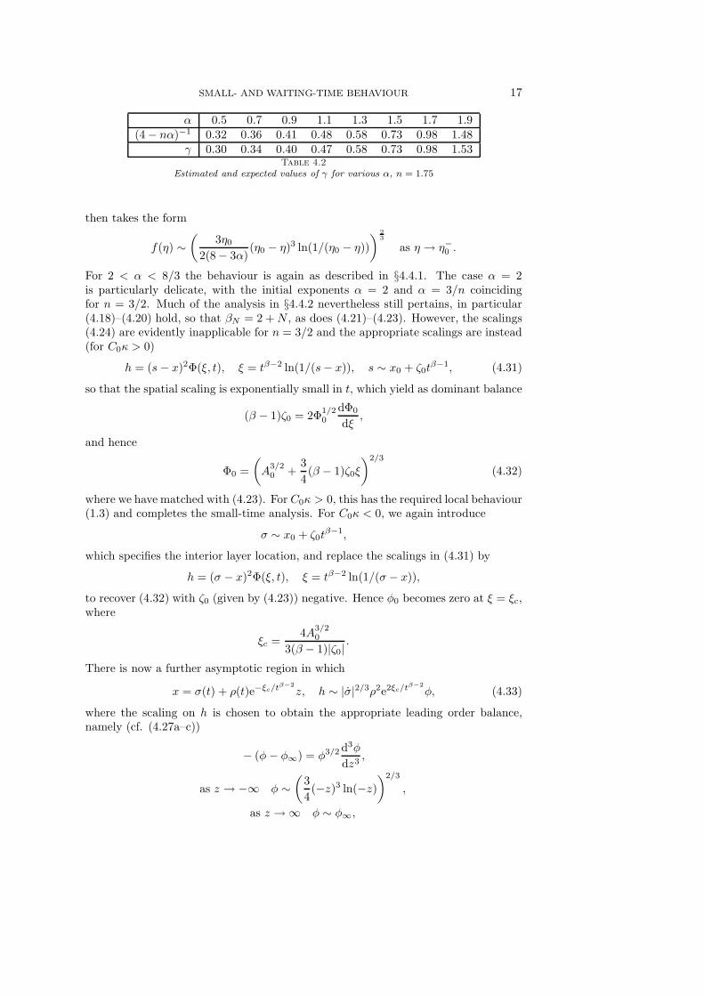
By monotonic decay we mean decay like η−γ , where γ is real, and by oscillatorydecay we mean that the solution decays like η−γ−iµ, where γ, µ are real. We presentnumerical results below for n = 0.75 (giving 3/n = 4, α2(n) = 4.2061, α5(n) = 4.9,4/n = 5.3333), with α = 5.1 (Figures 4.6 and 4.7), α = 4.5 (Figures 4.8 and 4.9) andα = 4.1 (Figures 4.10 and 4.11), thus covering each of the three parameter regimesdescribed above (see also Appendix A). We also present results for n = 1.0 (for whichα2(n) = 3.2195) with α = 3.1 (Figures 4.12 and 4.13), with this second example inthe range 3/n < α < α2 reflecting the extremely delicate nature of the results in thisregime.

0 0.1 0.2 0.3 0.4 0.5 0.6 0.7 0.8 0.9 1

x 10−3

0.7495

0.75

0.7505

0.751

0.7515

0.752

0.7525

0.753

0.6 0.65 0.70

0.2

0.4

0.6

0.8

1x 10

−4

tk=0

tk=1.0×10−4

tk=2.0×10−4

tk=3.0×10−4

tk

xk c

xj

Hk j

−8.5 −8 −7.5 −7 −6.5 −6 −5.5−45

−40

−35

−30

−25

tk=0

tk=2.5×10−5

tk=5.0×10−5

tk=7.5×10−5

−9 −8 −7 −6 −5 −4 −3 −2 −1 0−50

−40

−30

−20

−10

0

tk=0

tk=1.0×10−4

tk=2.0×10−4

tk=3.0×10−4

log(0.75 − xj)

log

Hk j

log(0.75 − xj)

log

Hk j

Fig. 4.6. Numerical results for n = 0.75, α = 5.1; waiting-time behaviour (upper left plot);profile of Hk

j near the interface at various times (lower left plot); log Hkj against log(xk

c −xj) in the

vicinity of the free boundary (upper right plot), and over the whole range xj ∈ [0, xkc ) (lower right

plot), with a dotted line of gradient 4/n (from asymptotic theory) in each case.

0.6 0.65 0.7 0.75 0.80

0.5

1

1.5

2

2.5

3x 10

−5

0.72 0.73 0.74 0.750

0.5

1

1.5

2

2.5

x 10−8

0.74 0.742 0.744 0.746 0.748 0.750

1

2

3

x 10−11

0.747 0.748 0.749 0.75 0.7510

0.2

0.4

0.6

0.8

1x 10

−13

tk=0

tk=4.0×10−4

tk=5.0×10−4

tk=6.0×10−4

xj

Hk j

xj

Hk j

xj

Hk j

xj

Hk j

Fig. 4.7. Numerical results for n = 0.75, α = 5.1; profile of Hkj near the interface at various

times (same legend for each plot).

In the upper left plots of Figures 4.6, 4.8, 4.10 and 4.12 we plot xkc against tk

for each example. In Figures 4.6 and 4.8, xkc remains stationary for a period before


0 0.1 0.2 0.3 0.4 0.5 0.6 0.7 0.8 0.9 1

x 10−3

0.749

0.75

0.751

0.752

0.753

0.754

0.755

0.756

0.64 0.66 0.68 0.7 0.72 0.740

0.5

1

1.5

2x 10

−5

tk=0

tk=1.0×10−4

tk=2.0×10−4

tk=3.0×10−4

tk

xk c

xj

Hk j

−9.5 −9 −8.5 −8 −7.5 −7 −6.5 −6 −5.5−50

−45

−40

−35

−30

−25

−20

tk=0

tk=2.5×10−5

tk=5.0×10−5

tk=7.5×10−5

−10 −9 −8 −7 −6 −5 −4 −3 −2 −1 0−50

−40

−30

−20

−10

0

tk=0

tk=1.0×10−4

tk=2.0×10−4

tk=3.0×10−4

log(0.75 − xj)

log

Hk j

log(0.75 − xj)lo

gH

k j

Fig. 4.8. Numerical results for n = 0.75, α = 4.5; waiting-time behaviour (upper left plot);profile of Hk

j near the interface at various times (lower left plot); log Hkj against log(xk

c −xj) in the

vicinity of the free boundary (upper right plot), and over the whole range xj ∈ [0, xkc ) (lower right

plot), with a dotted line of gradient 4/n (from asymptotic theory) in each case.

0.735 0.74 0.745 0.750

0.5

1

1.5

2x 10

−9

0.747 0.748 0.749 0.75 0.7510

1

2

3

4

5

x 10−13

0.62 0.64 0.66 0.68 0.7 0.72 0.74 0.760

1

2

3

4

5

6x 10

−6

tk=0

tk=4.0×10−4

tk=5.0×10−4

tk=6.0×10−4

xj

Hk j

xj

Hk j

xj

Hk j



advancing, with a shorter waiting period in Figure 4.8. In Figures 4.10 and 4.12, xkc

appears to immediately retreat, wait, and then advance. However, this retreat is overa very short distance, and over a longer timescale the boundary appears to wait; notethe different scales on the two plots in the upper left corner of Figure 4.12.

In the lower left corner of Figures 4.6, 4.8, 4.10 and 4.12 we show profiles ofHk

j in the vicinity of the free boundary at various times before the free boundary

has begun to advance. In each case the value of Hkj drops faster further behind the

free boundary, leading to the formation of humps near the boundary. In order todemonstrate the existence of more than one such hump, we show profiles of Hk

j onsmaller and smaller scales nearer and nearer to the free boundary in Figures 4.7, 4.9,4.11 and 4.13. Note the different scales on the horizontal and vertical axes of each


0 0.1 0.2 0.3 0.4 0.5 0.6 0.7 0.8 0.9 1

x 10−3

0.748

0.749

0.75

0.751

0.752

0.753

0.67 0.68 0.69 0.7 0.71 0.72 0.73 0.74 0.75 0.760

0.2

0.4

0.6

0.8

1x 10

−6

tk=0

tk=5.0×10−5

tk=1.0×10−4

tk=1.5×10−4

tk

xk c

xj

Hk j

−9.5 −9 −8.5 −8 −7.5 −7 −6.5 −6 −5.5−45

−40

−35

−30

−25

tk=1.0×10−4

tk=1.25×10−4

tk=1.5×10−4

tk=1.75×10−4

−10 −9 −8 −7 −6 −5 −4 −3 −2 −1 0−50

−40

−30

−20

−10

0

tk=1.0×10−4

tk=1.25×10−4

tk=1.5×10−4

tk=1.75×10−4

log(xkc − xj)

log

Hk j

log(xkc − xj)

log

Hk j

Fig. 4.10. Numerical results for n = 0.75, α = 4.1; motion of the numerical free boundary(upper left plot); profile of Hk

j near the interface at various times (lower left plot); log Hkj against

log(xkc − xj) in the vicinity of the free boundary (upper right plot), and over the whole range xj ∈

[0, xkc ) (lower right plot), with a dotted line of gradient 4/n (from asymptotic theory) in each case.

0.66 0.67 0.68 0.69 0.7 0.71 0.72 0.73 0.74 0.750

0.2

0.4

0.6

0.8

1x 10

−6

tk=1.0×10−4

tk=1.25×10−4

tk=1.5×10−4

tk=1.75×10−4

0.735 0.74 0.745 0.750

0.2

0.4

0.6

0.8

1x 10

−9

0.7465 0.747 0.7475 0.748 0.74850

0.2

0.4

0.6

0.8

1x 10

−12

xj

Hk j

xj

Hk j

xj

Hk j



plot in Figures 4.7, 4.9, 4.11 and 4.13

In the upper right corner of Figures 4.6, 4.8, 4.10 and 4.12 we plot log Hkj against

log(xkc − xj) in the vicinity of the free boundary at various times before the free

boundary has begun to advance. For comparison we also plot a dotted line with slope4/n in each figure. In Figure 4.6, the best fitting least squares line for tk = 0 has aslope of 5.10, rising to 5.26 for tk = 2.5 × 10−5 and 5.45 for tk = 5.0 × 10−5. Fortk = 7.5×10−5 the log-log plot is no longer very straight. We remark that in this casewith n = 0.75 and α = 5.1, Hk

j is very close to zero quite far behind the free boundary,hence the numerical results are extremely delicate. In Figure 4.8, the log-log plot isnot straight immediately in the vicinity of the free boundary for any tk > 0, althoughit is fairly straight further away from the free boundary. In Figures 4.10 and 4.12, the


0 1 2 3 4 5

x 10−3

0.72

0.74

0.76

0.78

0.8

0.82

0.84

0 0.2 0.4 0.6 0.8 1

x 10−3

0.749

0.7495

0.75

0.7505

0.751

0.715 0.72 0.725 0.73 0.735 0.74 0.745 0.750

0.2

0.4

0.6

0.8

1x 10

−5

tk=0

tk=5.0×10−5

tk=1.0×10−4

tk=2.0×10−4

tk

xk c

tk

xk c

xj

Hk j

−9.5 −9 −8.5 −8 −7.5 −7 −6.5 −6 −5.5−34

−32

−30

−28

−26

−24

−22

−20

−10 −9 −8 −7 −6 −5 −4 −3 −2 −1 0−40

−30

−20

−10

0

tk=3.0×10−4

tk=3.25×10−4

tk=3.5×10−4

tk=3.75×10−4

tk=3.0×10−4

tk=3.25×10−4

tk=3.5×10−4

tk=3.75×10−4

log(xkc − xj)

log

Hk j

log(xkc − xj)

log

Hk j

Fig. 4.12. Numerical results for n = 1.0, α = 3.1; motion of the numerical free boundary(upper left plots: note the different scales on each figure); profile of Hk

j near the interface at various

times (lower left plot); log Hkj against log(xk

c − xj) in the vicinity of the free boundary (upper right

plot), and over the whole range xj ∈ [0, xkc ) (lower right plot), with a dotted line of gradient 4/n

(from asymptotic theory) in each case.

0.7 0.705 0.71 0.715 0.72 0.725 0.73 0.735 0.74 0.745 0.750

0.5

1

1.5

2x 10

−6

tk=3.0×10−4

tk=3.25×10−4

tk=3.5×10−4

tk=3.75×10−4

0.744 0.745 0.746 0.747 0.748 0.749 0.750

0.5

1

1.5

2x 10

−9

xj

Hk j

xj

Hk j



log-log plots are not very straight, and the best fitting least squares lines have slopessignificantly lower than 4/n.

In the lower right corners of Figures 4.6, 4.8, 4.10 and 4.12 we plot log Hkj against

log(xkc −xj) over the whole range xj ∈ [0, xk

c ) at various times before the free boundaryhas begun to advance, plotting again a dotted line with slope 4/n for comparison. InFigure 4.6, as tk increases, the log-log plot becomes less and less straight, and fortk = 3.0 × 10−3 the periodic behaviour of the solution near the interface can clearlybe seen. The log-log plots for tk = 4.0× 10−3 and tk = 5.0× 10−3 are very similar tothat for tk = 3.0×10−3 but are not shown here. In Figure 4.8, the formation of humpsfurther and further from the free boundary becomes apparent. For tk = 1.0 × 10−4,


the slope of the log-log plot away from the free boundary is close to 4/n. For each ofFigures 4.10 and 4.12, as tk increases the formation of extra humps in the vicinity ofthe free boundary becomes apparent.

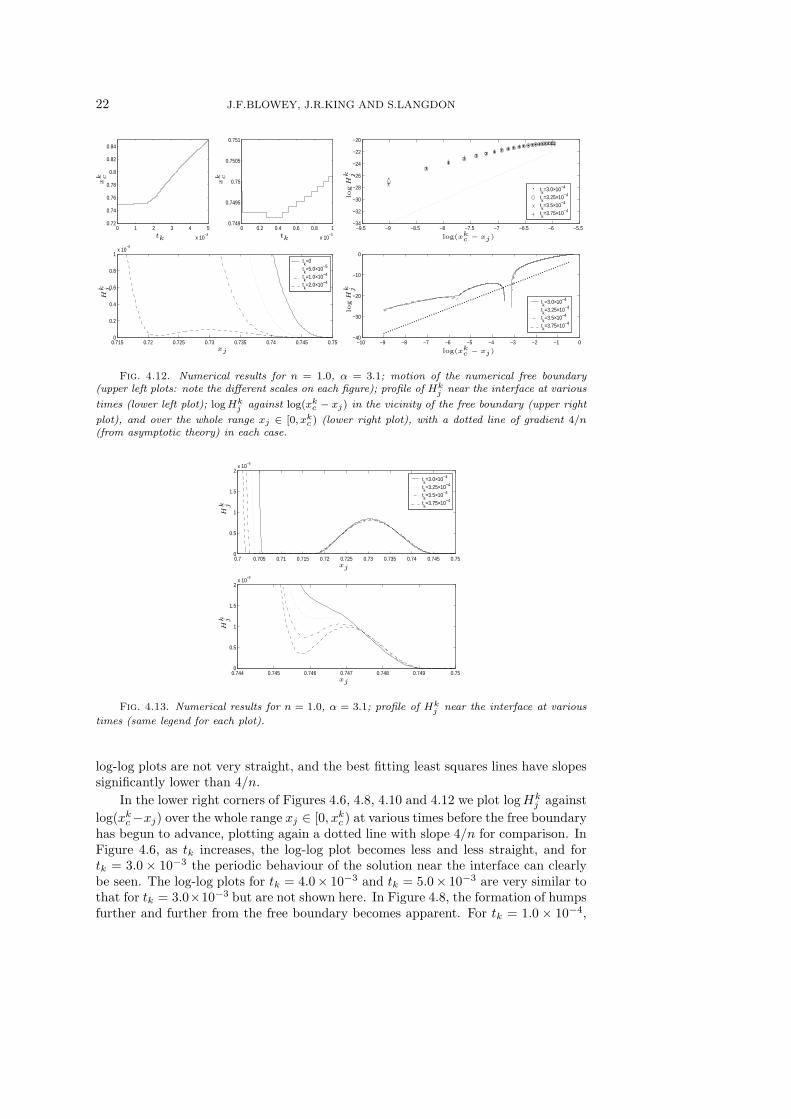
4.6.2. 2 < α < 3/n. To test the conjecture that the free boundary retreats in-stantaneously with unbounded velocity, we ran experiments with n = 1.0 and α ∈[2.1, 2.9]. We plot xk

c against tk in the left half of Figure 4.14 for α = 2.2, 2.4, 2.6and 2.8. The results support the conjecture. In each case the free boundary retreats,waits, and then advances, although the subsequent advance can only be seen in thefigure for α = 2.2. The initial velocity of xk

c appears to decrease as α increases, al-though as α increases the length of the period for which the free boundary retreatsalso increases, so that the maximum distance retreated occurs for α = 2.9.

0 0.1 0.2 0.3 0.4 0.5 0.6 0.7 0.8 0.9 1

x 10−4

0.73

0.735

0.74

0.745

0.75

0.755α=2.2α=2.4α=2.6α=2.8

tk

xk c

0 0.1 0.2 0.3 0.4 0.5 0.6 0.7 0.8 0.9 1

x 10−4

0.735

0.74

0.745

0.75

0.755

−17.5 −17 −16.5 −16 −15.5 −15 −14.5 −14 −13.5 −13−10

−9.5

−9

−8.5

−8

−7.5

−7

−6.5

tk

xk c

n = 1.0, α = 2.5

log tk

log(x0 c

−x

k c)

Fig. 4.14. Numerical results for n = 1.0, 2 < α < 3/n. In the left half of the figure we plot theretreating free boundary for various α. In the right half of the figure we show results for n = 1.0,α = 0.5: in the upper right section we show the retreating free boundary; in the lower right sectionwe plot log tk against log(x0

c − xkc ) as a discrete set of points, with the solid line following from a

least squares fitting and the straight dotted line from asymptotic theory.

As before we test the hypothesis xkc = x0

c − Atγk for some constants A > 0 and γby plotting log(x0

c −xkc ) against log tk. Again, if the hypothesis is correct we expect a

straight line with slope γ, and to estimate γ we take a least squares fit over the rangefor which the log–log plot is approximately straight. In the right half of Figure 4.14we plot xk

c against tk (upper section) and this log–log plot (lower section) for n = 1.0and α = 2.5. The log–log plot is approximately straight, and the best fitting leastsquares line is plotted as a solid line on the same figure. For comparison we also plota dotted line with slope (4− nα)−1 = 0.67. The estimated value of γ = 0.67 matchesthis exactly to two decimal places. The expected and estimated values of γ for eachvalue of α tested are shown in Table 4.3. The trend of γ increasing with α is clear,and away from the edges of the parameter regime the estimated value of γ is veryclose to the expected value.

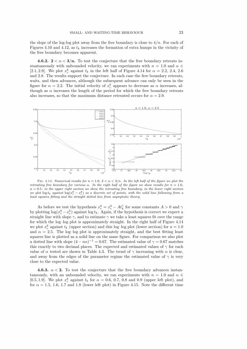
4.6.3. α < 2. To test the conjecture that the free boundary advances instan-taneously, with an unbounded velocity, we ran experiments with n = 1.0 and α ∈[0.5, 1.9]. We plot xk

c against tk for α = 0.6, 0.7, 0.8 and 0.9 (upper left plot), andfor α = 1.5, 1.6, 1.7 and 1.8 (lower left plot) in Figure 4.15. Note the different time


α 2.1 2.2 2.3 2.4 2.5 2.6 2.7 2.8 2.9(4 − nα)−1 0.53 0.56 0.59 0.63 0.67 0.71 0.77 0.83 0.91

γ 0.44 0.53 0.58 0.63 0.67 0.72 0.77 0.81 0.85Table 4.3

Estimated and expected values of γ for n = 1.0, various α

scales on the two plots. The results support the conjecture, and the initial velocity ofxk

c decreases as α increases.

0 0.1 0.2 0.3 0.4 0.5 0.6 0.7 0.8 0.9 1

x 10−9

0.75

0.751

0.752

0.753

0.754

0.755

0.756

0 0.1 0.2 0.3 0.4 0.5 0.6 0.7 0.8 0.9 1

x 10−5

0.75

0.755

0.76

0.765

0.77

α=0.6α=0.7α=0.8α=0.9

α=1.5α=1.6α=1.7α=1.8

tk

xk c

tk

xk c

0 0.1 0.2 0.3 0.4 0.5 0.6 0.7 0.8 0.9 1

x 10−7

0.75

0.751

0.752

0.753

0.754

0.755

0.756

−27 −26 −25 −24 −23 −22 −21 −20 −19 −18−9.5

−9

−8.5

−8

−7.5

−7

−6.5

−6

−5.5

tk

xk c

n = 1.0, α = 1.2

log tk

log(x

k c−

x0 c)

Fig. 4.15. n = 1.0, α < 2. In the left half of the figure we plot the advancing free boundary forvarious α (note the different time scales on the two plots). In the right half of the figure we showresults for n = 1.0, α = 1.2: in the upper right section we show the advancing free boundary; in thelower right section we plot log tk against log(xk

c − x0c) as a discrete set of points, with the solid line

following from a least squares fitting and the straight dotted line from asymptotic theory.

We again test the hypothesis (4.11), plotting xkc against tk (upper right section

of Figure 4.15) and log(xkc − x0

c) against log tk (lower right section of Figure 4.15)for n = 1.0 and α = 1.2. The log–log plot is approximately straight, and the bestfitting least squares line, plotted as a solid line on the same figure, has a slope of 0.34.For comparison we also plot a dotted line with slope (4 − nα)−1 = 0.36 on the samefigure. The expected and estimated values of γ are shown in Table 4.4. The trend ofγ increasing with α is clear, and for values of α away from the borderline value α = 2the estimated value of γ is very close to the expected value.

α 0.5 0.7 0.9 1.1 1.3 1.5 1.7 1.9(4 − nα)−1 0.29 0.30 0.32 0.34 0.37 0.40 0.43 0.48

γ 0.28 0.29 0.31 0.33 0.36 0.40 0.43 0.53Table 4.4

Estimated and expected values of γ for n = 1.0, various α < 2

5. Conclusions. As we have seen, the thin-film equation (1.1a) exhibits a muchbroader range of small-time phenomena than its second order analogue, (1.6). Thus,while the behaviour of the former with 2 < n < 3 corresponds very closely to thatof the latter with any n > 0, for n < 2 equation (1.1a) exhibits a range of α in


which the interface waits but the local profile changes instantaneously from that ofthe initial data (this combination does not occur for (1.6)), and can exhibit monotonicor oscillatory decay to the local solution (4.14) or limit-cycle behaviour of the form(A.5). Moreover, for n < 3/2 fronts can either advance or retreat and our small timeclassification gives rather precise criteria on the initial data in this regard. The verydelicate interlacing of initial profiles leading to immediate expansion or to a finitewaiting time, as outlined in §4.4.2, for example, also deserves highlighting.

The high order problem (1.1) is a demanding one from the numerical point ofview; this wealth of distinct behaviours occurring over short length and time scalesnecessitates particularly refined, careful and detailed computational studies if therelevant phenomena are to be captured adequately, and we have sought to implementthe required programme of extensive numerical investigations.

A number of generalisations immediately suggest themselves. In higher dimen-sions, the small-time behaviour of an initially smooth interface will be locally one-dimensional, so most of the conclusions carry over. For n ≥ 3, the smoothest solutionshave fixed interfaces and here waiting-time phenomena relate (for 3 ≤ n < 4) to adelay in the contact angle becoming finite; we shall not elaborate on such mattershere, noting only that the approaches we have described above apply equally wellin such contexts. As a final instance, we note that for n < 3 a finite contact anglecondition can be imposed in place of the second of (1.1c) and a similar investigationperformed; again, we shall not report the results of such a study here.

REFERENCES

[1] S. Angenent, Solutions of the one-dimensional porous-medium equation are determined bytheir free boundary, J. London Math. Soc, 42 (1990), pp. 339–353.

[2] J. W. Barrett, J. F. Blowey, and H. Garcke, Finite element approximation of a fourthorder nonlinear degenerate parabolic equation, Numer. Math., 80 (1998), pp. 525–556.

[3] J. W. Barrett and S. Langdon, A multigrid method for a fourth order elliptic system. (inpreparation).

[4] J. Becker and G. Grun, The thin-film equation: recent advances and some new perspectives,J. Phys. Condens. Matter, 17 (2005), pp. S291–S307.

[5] E. Beretta, M. Bertsch, and R. Dal Passo, Nonnegative solutions of a 4th-order nonlineardegenerate parabolic equation, Arch. Ration. Mech. Anal., 129 (1995), pp. 175–200.

[6] F. Bernis, Viscous flows, fourth order nonlinear degenerate parabolic equations and singularelliptic problems, in Free boundary problems: theory and applications, A. L. J. I. Diaz, M.A. Herrero and J. L. Vazquez, eds., vol. 323 of Pitman Research Notes in Mathematics,Longman, Harlow, 1995, pp. 40–56.

[7] , Finite speed of propagation and continuity of the interface for thin viscous flows, Adv.in Diff. Equations, 1 (1996), pp. 337–368.

[8] , Finite speed of propagation for thin viscous flows when 2 ≤ n < 3, C. R. Acad. Sci.Paris; Ser. I Math., 322 (1996), pp. 1169–1174.

[9] F. Bernis and A. Friedman, Higher order nonlinear degenerate parabolic equations, J. Dif-ferential Equations, 83 (1990), pp. 179–206.

[10] A. L. Bertozzi, Symmetric singularity formation in lubrication-type equations for interfacemotion, SIAM J. Appl. Math., 56 (1996), pp. 681–714.

[11] , The mathematics of moving contact lines in thin liquid films, Notices of the AMS, 45(1998), pp. 689–697.

[12] A. L. Bertozzi, M. P. Brenner, T. F. Dupont, and L. P. Kadanoff, Singularities and simi-larities in interface flows, in Trends and Perspectives in Applied Mathematics, L. Sirovich,ed., vol. 100 of Appl. Math. Sci., Springer-Verlag, New York, 1994, pp. 155–209.

[13] A. L. Bertozzi, G. Grun, and T. P. Witelski, Dewetting films: bifurcations and concentra-tions, Nonlinearity, 14 (2001), pp. 1569–1592.

[14] A. L. Bertozzi and M. Pugh, The lubrication approximation for thin viscous films: regularityand long time behaviour of weak solutions., Comm. Pure Appl. Math., 49 (1996), pp. 85–123.


[15] J. F. Blowey, J. R. King, and S. Langdon, Small- and waiting-time behaviour of the thin-film equation. Brunel University Department of Mathematical Sciences Technical ReportTR/03/03, 2003.

[16] R. Dal Passo, H. Garcke, and G. Grun, On a fourth order degenerate parabolic equation:global entropy estimates and qualitative behaviour of solutions, SIAM J. Math. Anal., 29(1998), pp. 321–342.

[17] R. Dal Passo, L. Giacomelli, and G. Grun, A waiting time phenomenon for thin filmequations, Ann. Scuola Norm. Sup. Pisa Cl. Sci., 30 (2001), pp. 437–463.

[18] E. B. Dussan and S. H. Davis, On the motion of a fluid-fluid interface along solid surface, J.Fluid Mech., 65 (1974), pp. 71–95.

[19] H. P. Greenspan, On the motion of a small viscous droplet that wets a surface, J. Fluid Mech.,84 (1978), pp. 125–143.

[20] G. Grun, Droplet spreading under weak slippage: the waiting time phenomenon, Ann. Inst. H.Poincare Anal. Non Lineaire, 21 (2004), pp. 255–269.

[21] G. Grun and M. Rumpf, Nonnegativity preserving convergent schemes for the thin film equa-tion, Numer. Math., 87 (2000), pp. 113–152.

[22] R. E. Grundy, Local similarity solutions for the initial-value problem in non-linear diffusion,IMA J. Appl. Math., 30 (1983), pp. 209–214.

[23] L. M. Hocking, Sliding and spreading of thin two-dimensional drops, Quart. J. Mech. Appl.Math., 34 (1981), pp. 37–55.

[24] E. Huh and L. E. Scriven, Hydrodynamic model of steady movement of a solid / liquid /fluid contact line, J. Colloid Interface Sci., 35 (1971), pp. 85–101.

[25] J. R. King, Exact polynomial solutions to some nonlinear diffusion equations, Phys. D, 64(1993), pp. 35–65.

[26] , Development of singularities in some moving boundary problems, European J. Appl.Math., 6 (1995), pp. 491–507.

[27] J. R. King and M. Bowen, Moving boundary problems and non-uniqueness for the thin filmequation, European J. Appl. Math., 12 (2001), pp. 321–356.

[28] A. A. Lacey, Initial motion of the free-boundary for a non-linear diffusion equation, IMA J.Appl. Math., 31 (1983), pp. 113–119.

[29] A. A. Lacey, J. R. Ockendon, and A. B. Tayler, Waiting-time solutions of a nonlineardiffusion equation, SIAM J. Appl. Math., 42 (1982), pp. 1252–1264.

[30] T. G. Myers, Thin films with high surface tension, SIAM Rev., 40 (1998), pp. 441–462.

Appendix A. Applicability of the local solution (4.4). In this appendixwe use boundary condition counting arguments to assess the applicability of (4.4) asa local solution to (4.2) for 0 < n < 2. Writing

f ∼(

n3

8(4 − n)(2 − n)(n + 4)(−η)4

) 1n

+ F (A.1)

and linearising yields

1

4 − nα(αF − ηFη) = − n3

8(4 − n)(2 − n)(n + 4)

d

dη

(η4 d3F

dη3

)− n

n + 4

d

dη(ηF ) ,

with solutions

F = K(−η)p (A.2)

where the possible p are the roots of the quartic

n3p(p − 1)(p − 2)(p + 1)

8(4 − n)(2 − n)(n + 4)+

n(p + 1)

n + 4+

α − p

4 − nα= 0. (A.3)

The expansion of (A.1) with F given by (A.2) is self-consistent if Re(p) > 4/n, so therelations between α and n such that two roots of (A.3) have Re(p) = 4/n are crucial;these relations can be shown to be

α1(n) =α−b + α∆

αd, α2(n) =

α−b − α∆

αd,


where

αd = 2(n2 − n − 8

) (7 n3 − 84 n2 + 400 n− 640

)n,

α−b = 47n5 − 674n4 + 3384n3 − 3520n2 − 17408n + 36864,

α∆ = (n + 4)(2 − n)(8 − n)√

9216− 5632n + 896n2 + 112n3 − 31n4,

so that

α1∼2 +11

10(2 − n) + O

((2 − n)

2)

as n → 2−, α1∼3

n+

5

24+ O (n) as n → 0+,

α2∼2 +31

22(2 − n)

2+ O

((2 − n)

3)

as n → 2−, α2∼21

5n− 1

120+ O(n) as n → 0+.

It is also instructive to note the curves in (α, n) space on which roots of (A.3) becomecomplex, namely the repeated roots case in which (A.3) and

d

dp

[n3p(p − 1)(p − 2)(p + 1)

8(4 − n)(2 − n)(n + 4)+

n(p + 1)

n + 4+

α − p

4 − nα

]= 0 (A.4)

are satisfied simultaneously. The various curves relevant to our discussion are shownin Figure A.1. In particular we define α5 = α5(n) to be the repeated root case (vb)shown in Figure A.1.

0 0.2 0.4 0.6 0.8 1 1.2 1.4 1.6 1.8 2n0

0.5

1

1.5

2

2.5

3

3.5

4

α

(ϖe)

(vc)

(vd)

(va)

(vb)

(i)

(ii)

(iii)

(iv)

4

5

6

7

8

9

10

0.2 0.4 0.6 0.8 1n

α

Fig. A.1. (α, n) space; (i) α = α1, (ii) α = 4/n, (iii) α = α2, (iv) α = 3/n, (v) the solutionsto (A.3) and (A.4). To the right of (va) and of the right most of (vd) and (ve) there are four realroots; between (va) and (vb), between (vd) and (ve) and to the left of (vc) there are two real andtwo complex roots; between (vc), (vb) and the left most of (vd) and (ve) there are four complexroots. Three of the roots become unbounded as (ii) is approached, with the fourth having p ∼ 4/n.Above (i) and below (iii), none of the roots have Re(p) > 4/n; between (iii) and (vb), two of thefour complex roots have Re(p) > 4/n and the other two Re(p) < 4/n; between (vb) and (ii) both realroots satisfy p > 4/n and both complex ones Re(p) < 4/n; between (ii) and (i) the real roots havep < 4/n and the complex ones Re(p) > 4/n.

In α2 < α < 4n , two roots of (A.3) have Re(p) > 4

n and the local expansion (A.1)is correctly specified (the two degrees of freedom being the K’s in (A.2) correspondingto those two roots). As α drops below α2 we anticipate that a Hopf bifurcation occurs


in (4.2)–(4.3a,b) with the local behaviour as η → 0− taking for α > max(2, 3/n) the“limit-cycle” form

f ∼ (−η)4n Ω(− ln(−η)) (A.5)

where Ω(ξ) is periodic of period P , say, in ξ. Since on α = α2

Im(p) = ± 1√2n

√96 − 24n− n2 −

√9216− 5632n + 896n2 + 112n3 − 31n4,

we anticipate that

P ∼ 2√

2πn√96 − 24n− n2 −

√9216− 5632n + 896n2 + 112n3 − 31n4

as α → α−

2 .

Note that P will depend on α and n but, in view of the scaling properties of (4.2)–(4.3a,b), not on A0. For α5 < α < 4

n , the decay to (4.4) is non-oscillatory while forα2 < α < α5 damped oscillations occur.

Appendix B. 3/2 < n < 2, α → 2. We are concerned here with the behaviourof (4.2)-(4.3a,b) for α close to two. Writing α = 2 + ǫ, 0 < |ǫ| ≪ 1, we have forη = O(1) that

f ∼ A0(−η)2 + ǫf1(η) (B.1)

with

1

2(2 − n)

(2f1 − η

df1

dη+ A0(−η)2

)= −An

0

d

dη

((−η)2n d3f1

dη3

), (B.2a)

as η → −∞ f1 ∼ A0(−η)2 ln(−η) − 2(2n − 1)An+10 (−η)2(n−1), (B.2b)

as η → 0− f1 = (−η)2n d3f1

dη3= 0. (B.2c)

It follows from (B.2a–c) that

f1 ∼ −µ(n)A4−n

2(2−n)

0 (−η) as η → 0+; (B.3)

we believe the constant µ, which is determined as part of the solution to (B.2a–c), to

be positive; the dependence on A0 in (B.3) follows from rescaling f1 by A2/(2−n)0 and

η by An/(2(2−n))0 in (B.2a–c).

The expansion (B.1) breaks down for small η with inner scalings η = |ǫ|ξ, f =

|ǫ|2g(ξ) and ddξ

(gn0

d3g0

dξ3

)= 0. For ǫ < 0 we thus have

g0 = A0(ξ0 − ξ)2, ξ0 =1

2µA

n2(2−n)

0 , (B.4)

with η0 ∼ |ǫ|ξ0 and with inner-inner scalings η = η0 + |ǫ|1/(2n−3)ζ, f = |ǫ|2/(2n−3)h(ζ),whereby

1

2(2 − n)ξ0 = hn−1

0

d3h0

dζ3,

as ζ → −∞ h0 ∼ A0(−ζ)2,

as ζ → 0− h0 ∼(

n3ξ0

6(3 − n)(2n − 3)(2 − n)(−ζ)3

) 1n

,


producing the desired local behaviour (1.2). However, for ǫ > 0 the expression (B.4)is replaced by

g0 = A0(−ξ0 − ξ)2, ξ0 =1

2µA

n2(2−n)

0 , (B.5)

and (recalling that the interface cannot contract for n > 3/2) the inner-inner scalingsread ξ = −ξc(ǫ) + ǫ2(2−n)/(2n−3)ζ, g = ǫ4(2−n)/(2n−3)h(ζ), where ξc(0) = ξ0 and

− 1

2(2 − n)ξ0(h0 − H∞) = hn

0

d3h0

dζ3, (B.6a)

as ζ → −∞ h0 ∼ A0(−ζ)2, (B.6b)

as ζ → ∞ h0 → H∞, (B.6c)

which determines both h0 (up to translations in ζ) and H∞, the decay of h0 to H∞

being non-oscillatory. In −ξ0 < ξ < 0 we then have

h ∼ H∞

(−ξ)2

ξ20

, (B.7)

the left-hand side of (4.2) dominating. The scaling properties of (B.6a–c) show that

h0 and H∞ scale with A2/(2−n)0 and ζ with A

n/(2(2−n))0 , so we may rewrite (B.7) as

h ∼ ν(n)A0(−ξ)2. (B.8)

Now setting

f = ν2

2−n ǫ8

2n−3 f , η = νn

2(2−n) ǫ2n

2n−3 η, (B.9)

we have that

f ∼ A0(−η)2 + ǫf1(η),

where f1 satisfies (B.2a–c) with η replaced by η, implying that the above structurerepeats itself on a sequence of finer and finer scales, consistent with the limit cyclebehaviour referred to in Appendix A. Thus if we denote the variables in the mthmember of the sequence by f (m), η(m) with f (0) = f and η(0) = η we have from (B.9)that

f (m) ∼ ν2

2−n ǫ8

2n−3 f (m−1), η(m) ∼ νn

2(2−n) ǫ2n

2n−3 η(m−1),

implying that

f (m)(η) ∼ ν2m2−n ǫ

8m2n−3 f

(η

νmn

2(2−n) ǫ2mn2n−3

),

where leading order expressions for f on the right-hand side are given through a singlecycle of the oscillation by (B.1), (B.5), (B.6a–c), (B.8). This is consistent with (A.5)with

P ∼ 2n

2n − 3ln

(1

ǫ

)− n

2(2 − n)ln ν

being large; note that the region described by (B.6a–c) is particularly significantbecause it leads to the (−η)4/n type decay in (A.5) despite the solution behavingquadratically in other regions.

small- and waiting-time behaviour of the thin-film

Documents