Upjohn Institute Working Papers Upjohn Research home page

6-1-2004

Small Cities Blues: Looking for Growth Factors in Small and Small Cities Blues: Looking for Growth Factors in Small and

Medium-Sized Cities Medium-Sized Cities

George A. Erickcek W.E. Upjohn Institute for Employment Research, erickcek@upjohn.org

Hannah J. McKinney Kalamazoo College

Upjohn Institute Working Paper No. 04-100

**Published Version**

In Economic Development Quarterly, 20(3): 232-258 (2006).

Follow this and additional works at: https://research.upjohn.org/up_workingpapers

Part of the Labor Economics Commons, and the Urban Studies and Planning Commons

Citation Citation Erickcek, George A. and Hannah McKinney. "Small Cities Blues: Looking for Growth Factors in Small and Medium-Sized Cities." Upjohn Institute Working Paper No. 04-100. Kalamazoo, MI: W.E. Upjohn Institute for Employment Research. https://doi.org/10.17848/wp04-100

This title is brought to you by the Upjohn Institute. For more information, please contact repository@upjohn.org.

“Small Cities Blues”: Looking for Growth Factorsin Small and Medium-Sized Cities

Upjohn Institute Staff Working Paper No. 04-100

June 2004

George A. ErickcekUpjohn Institute for Employment Research

and

Hannah McKinneyKalamazoo College

JEL Code: R110

******************************************************************************We wish to thank Brad Watts for his outstanding research assistance.******************************************************************************

Small Cities Blues: Looking for Growth Factors inSmall and Medium-Sized Cities

Abstract

The purpose of this exploratory study is to attempt to identify particular public policieswhich have the potential to increase the economic viability of smaller metropolitan areas and cities.We identify characteristics associated with smaller metro areas that performed better-than-expected(winners) and worse-than-expected (losers) during the 1990s, given their resources, industrial mix,and location as of 1990. Once these characteristics have been identified, we look for evidence thatpublic policy choices may have promoted and enhanced a metro area’s ability to succeed and toregain control of its own economic destiny. Methodologically, we construct a regression modelwhich identifies the small metro areas that achieved higher-than-expected economic prosperity(winners) and the areas that saw lower-than-expected economic prosperity (losers) according to themodel. Next, we explore whether indications exist that winners and losers are qualitatively differentfrom other areas in ways that may indicate consequences of policy choices. A cluster analysis iscompleted to group the metro areas based on changes in a host of social, economic, anddemographic variables between 1990 and 2000. We then use contingency table analysis andANOVA to see if “winning” or “losing,” as measured by the error term from the regression, isrelated to the grouping of metro areas in a way that may indicate the presence of deliberate andreplicable government policy.

1Betty Flores, Mayor of Laredo, in a letter available at: http://usmayors.org/uscm/buscouncile/default.asp.

INTRODUCTIONIn today’s dynamic global economy, smaller metropolitan areas in the United States have

lost much of their economic role and vitality. These areas often are held hostage to decisions madein large company boardrooms (Watts and Kirkham 1999). In particular, in the wake of corporatemergers, many areas are becoming branch plant production locations that, in turn, do not generatea social or civic environment attractive to professional workers. Moreover, because of mergers andclosures, these areas often lose key private sector stakeholders who, in the past, would have beenmajor players in creating and implementing public and private policies to bolster the area againstthe negative impacts of downsizing and relocations of major employers. In short, some questionwhether these smaller places really have a role in today’s global economy (Kelley 1996; Glaeser andShapiro 2003).

Yet, mayors of all sizes of cities firmly believe that “now, more than ever, the continuedvitality of cities and the nation are dependent upon mayors and private sector leaders tackling issuesof common concern such as, but not limited to: streamlining government, providing homelandsecurity and public safety, building affordable housing, investing in kids and schools, promoting thearts, culture, and sports, recycling land and preserving open spaces, investing tax cuts in challengedneighborhoods and working families, workforce training, modernizing infrastructure, and increasingaccess to affordable healthcare.”1

The purpose of this study is to see whether statistical evidence exists to suggest thatparticular public policies can increase the economic viability of metropolitan areas and cities. Weidentify characteristics associated with smaller metro areas that performed better than expected(winners) and worse than expected (losers) during the 1990s given their resources, industrial mix,and location as of 1990. Once these characteristics are identified, we look for evidence that publicpolicy choices may have promoted and enhanced a metro area’s ability to succeed and to regaincontrol of its own economic destiny. First, we construct a regression model that we use to forecastthe growth of metropolitan areas during the 1990s. Then we identify the small metro areas thatachieved higher-than-expected economic prosperity (winners) and the areas that saw lower-than-expected economic prosperity (losers) according to the model. The regression model includes a shiftshare variable plus a variety of trend and condition variables, all measured as of 1990. Theunexplained portion of growth is captured in the error term from the regression.

Next, we explore whether indications exist that winners and losers are qualitatively differentfrom other areas in ways that may indicate consequences of policy choices. We do a variety ofstatistical tests, using the error term as the dependent variable, to examine this question. Variablesused in these tests are all measured for 2000, or as changes in their levels from 1990 to 2000. The

2

first test is a regression that uses city public-finance variables as the regressors. Next a clusteranalysis is completed to group the metro areas based on changes in a host of social, economic, anddemographic variables between 1990 and 2000. We then use contingency table analysis andANOVA to see if “winning” or “losing,” as measured by the error term from the regression, isrelated to the grouping of metro areas in a way that may indicate the presence of deliberate andreplicable government policy.

We recognize that a metro area’s success, of lack thereof, could be as simple as the recentbirth of a Fortune 500 company or a series of plant openings or closings (see Barrow and Hall 1995;Palmer 1994; Foust 2003). Yet, some areas may be pursuing policies that are transferable, yieldtangible results, and may be key to revitalizing many of our metropolitan areas. This paper is thefirst step toward our ultimate research goal: to identify these transferable activities.

LITERATURE REVIEWThe Current Economic Environment Facing Small Metropolitan Areas

Case studies have documented the impact of the loss of a major industrial employer on acommunity (Kirsch 1998; Teaford 1994). Smaller metro areas have fewer resiliencies againsteconomic downturns and plant closings or major downsizings (Siegel and Waxman 2001). Theprivate industry leadership pool disappears. An emotional and civic void is created, and it is likelythat most smaller areas lack the economic capacity necessary to weather the shutdown or downsizingof these major employers. The several thousand workers who lose their jobs all at once are notreabsorbed easily or quickly into the local labor market (Moore 1996).

Amenities, particularly cultural entities and events, are supposed to stimulate the growth ofcities both large and small (Moses 2001; Fulton and Shigley 2001; Gottleib 1995). Small metroareas may lack growth-facilitating amenities, especially for professional workers. According toFlorida (2002), small metro areas are held back not because they lack impressive art museums ormajor league sports teams, but because of their manufacturing heritage or culture, lack of andintolerance of diversity, and aging population. More and more young professionals see small metroareas as “fly-overs.” While, older professionals may see small metro areas as nice places to raisetheir families; however, they may not be as entrepreneurial as the younger population.

Review of Past StudiesSiegel and Waxman (2001) point to six challenges for small cities: 1) out-of-date

infrastructure, 2) dependence on traditional industry, 3) obsolete human capital base, 4) decliningregional competitiveness, 5) weakened civic infrastructure and capacity, and 6) limited access toresources. In much of the recent literature on urban growth, the benefits of urban

3

agglomeration—particularly that of industrial clustering—still hold center stage (Krugman 1998;O hUallachain 1999; Mayer and Greenberg 2001; Camagni 2002; Porter 2000, 2003). This is incontrast to earlier times, when decentralization caused by decreasing transportation andcommunication costs was considered the norm (Zelinsky 1962). Lovering (1999) discusses thedearth of empirical studies of the causes of urban economic growth.

One of the existing gaps in the research that we hope to fill is that most of the recent workon economic growth and transition in American urban areas has concentrated on large metroareas—those with 1 million or more in population (Glaeser and Shapiro 2003a, b; Berube 2003;Pack 2002; Gottlieb 2001). Very few studies of small metro areas exist and most of them are casestudies. (For instance, through a series of interviews with local officials, Mayer and Greenberg(2001) examined 34 small cities that had suffered a major plant closing to see how they fared in theyears after the event.) Still, regardless of methodology, almost all studies show that on a numberof measurable scales, such as unemployment and poverty rates or population decreases, smallercities are losing their economic viability in the new global economy (U.S. Department of Housingand Urban Development 1999; Erhlick 2000; Raymond and Pascarella 1987). Moreover, ifagglomeration or clustering is an important precursor to growth, smaller areas may be at adisadvantage in their ability to use policy to reshape their economies. Data limitations have beenone reason for the paucity of empirical studies of small areas (Smith 1990).

On the other hand, some researchers doubt that a city’s size, by itself, is as important as thelack of economic structure and networks that are likely found in larger metropolitan areas (Wojanand Pulver 1995; Gabaix 1999). Bee (2003) also argues that size may not matter, yet finds that theexistence of large corporate research and development centers is a key to growth. Small metro areasare unlikely to have such centers. Similarly, in a study of the largest 150 metro areas, Anselin Vargaand Acs (1997) find that knowledge spillovers from universities only occur when an area has a denseintellectual infrastructure already in place. For a conflicting view of knowledge spillovers and citygrowth, see Glaeser et al. (1992).

Unfortunately for small metro areas, evidence on their potential cost advantages formanufacturing activity is mixed. Martin, McHugh and Johnson (1991) speculate that manufacturingis still sensitive enough to locational size advantages that economic development policy can betargeted to specific industries for specific places. Yet, evidence that large firms respond toagglomeration economies abounds. For instance, Shilton and Stanley (1999), in a study of 5,189headquarters of large U.S. firms, found that 40 percent were located in 20 counties, includingCalifornia’s Orange County (Los Angeles) and Santa Clara County (Silicon Valley). Changes intransportation and telecommunication technology have not led to decentralization of employment

4

from larger metro areas to smaller ones or non-metro areas; instead, professional and managerialoccupations tend to be concentrated in larger metro areas (Cook Kirschner, and Beck 1991).

DEVELOPMENT OF A PREDICTIVE MODELIn constructing the predictive model for the growth of metro areas between 1990 and 2000,

and particularly in the selection of structural variables, we relied heavily on the product cycle theoryof economic growth (Markusen 1985). The product cycle model suggests that a region’s economicperformance depends upon the “product age” of its primary export-base industries. Areas withexport- base firms that are producing mature or commodity-grade products or services are expectedto grow more slowly than areas with high-profit firms producing more cutting-edge products thatface less cost-based competition while enjoying expanding markets. Quite often these high-profitfirms are proprietorships and are small in size, employing between 20 and 40 workers. However,they are not the micro-employers (firms employing fewer than 20 workers). In fact, according tothe standard product-cycle model, little employment growth can be expected from an area’s smallestexport-base firms, as they are still testing the marketability of their product or service.

However, Plummer and Taylor (2001a, b) examined and contrasted the performance of sixtheoretical models of regional economic performance, including the product-cycle model, and foundthat none of variables they used as proxies for theoretical models explained much of the differencein regional performance, as defined by unemployment rate differentials. Still, the “learning regions”variables did the best, although these may be pointing to the importance of an area’s enterpriseculture based on a combination of entrepreneurship and a strong human-resource base instead of aformal learning process. Glaeser and Shapiro (2003b) examined population growth trends duringthe 1970s and 1980s and found that population trends in the 1990s were not significantly differentfrom those of past decades. Still, they also found that an area’s weather and human capital assetsmatter. Because of these two studies, we also used a variable to capture the areas’ quality of humancapital and climate.

Description of the ModelAgain, the objective of the regression analysis is to identify the key factors that contributed

to the growth of small and medium-sized cities during the 1990s. After we construct the model, weuse it to identify the metropolitan areas that outperformed or underperformed expectations. Our dataset was limited to the 267 metro areas that had populations of 1 million or less in 1990. Weperformed a Chow test on our regression, using these 267 areas as a subset of the 318 metropolitanareas defined by the Bureau of Economic Analysis for the United States. The Chow test showed thatthe regression results for smaller areas are significantly different from those for all areas.

2We did run the model using the percentage change in employment during the 1990s as the dependent variable.The results were very similar to the model used: the simple correlation between resulting lists of winning and losingmetro areas was 0.77.

5

Selecting the proper dependent variable in this study was no easy task. An ideal measurewould capture increases in the capacity to improve the quality of life within the area as well asimprovements in the quality of life. After much debate, we chose as our measure of economicgrowth the percentage change in personal income for the period 1989 to 1999. We also consideredusing changes in population, employment, and per capita income. We eliminated population changebecause population gains can be associated with congestion and increased demand for governmentservices without accompanying increases in revenue, thus diminishing an area’s quality of life.Employment growth as a measure of economic performance does not address the issue of the qualityof jobs being generated.2

As manufacturing has declined, job growth in many urban areas has come primarily in othersectors that typically pay lower wages (U.S. Conference of Mayors 2004). Change in per capitaincome was not used because we feared it could yield a “false positive” and because it does notreflect the total financial resources that are available to the local government. An area can have anincrease in per capita income while at the same time suffering a declining economic or resourcebase. If the area’s economy is both stagnating and highly dependent on one or two high-wageemployers, then as unemployed people leave the area, its per capita income can rise. On the otherhand, if the same area was growing but the new jobs being created were in small, innovativebusinesses that paid relatively low wages, its overall per capita income could fall. While totalincome growth is not a perfect measure, it does reflect an increase in the financial capacity of localgovernments to address quality of life issues.

The growth of a metropolitan area depends upon its economic structure, human capitalresources, quality of life factors, historical trends and, of course, location. The variables used asproxies for each of these factors are discussed below. Descriptive statistics for them are given inTable 1 below.

Structural VariablesWe used four variables to estimate the impact of the region’s industrial structure on its

growth during the 1990s. The first variable is the industrial mix component of a standard shift-sharemodel. The standard shift-share model divides an area’s growth into three components: 1) Nationaltrend, 2)Industrial mix and 3)Competitive share. National trend captures the portion of an area’sgrowth that can be attributed to the general growth of the national economy during the period. The

Table 1 Descriptive Statistics for Variables in Predictive Equation

Mean Median Maximum MinimumStandarddeviation

Structural variablesIndustrial shift, 1989 to 1999 ($ 000) !199529 !139075 1144523 !2911987 320667% businesses employing fewer than 20 workers in 1990 33.3 32.2 54.6 19.2 6.3% businesses employing between 20 and 49 workers in 1990 20.2 19.7 51.8 13.4 3.4% chg in proprietors’ income, 1980–1990 79.7 75.8 299 7.2 0.379

Human capital variables% residents, 25 or older, w/ college education in 1990 19.1 17.5 44 9.5 6.3

Quality of life variablesAverage July temperature (degrees) 56.6 54.8 77.5 36.3 8.5Annual precipitation (inches) 37.5 38.7 66.3 3 14Burglaries per 100,000 residents, 1992 2765 1702 17604 98 2883Larcenies per 100,000 residents, 1992 8384 5718 42616 321 735

Historical trends variablesPer capita income, 1989 16539 16184 28068 8691 2630% chg in metro poverty rate, 1979–1989 21.2 19.3 90 !58.5 0.237% chg in population, 1979–1989 11.5 8 89.8 !14.8 0.155SOURCE: All data are from U.S. Census 1990 or 1980 except: Industrial shift, calculated from REIS data from the BEA; % business employment, estimates based on data from the1990 County Business Patterns; climate data from the National Climate Data Center; and crime data from FBI reports.

7

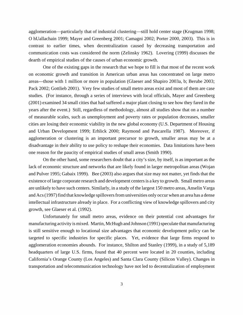
industrial mix captures that portion of an area’s growth that can be attributed to having a higher (orlower) share of the nation’s best-performing industries. If an area is lucky to have a highconcentration of industries that are enjoying strong national growth then, regardless of the relativeperformance of its firms in those industries, it can expect to do better than if it were stuck with ahigh concentration of industries that were suffering declining national markets. The finalcomponent, Competitive share, captures the area’s growth that can be attributed to its firms doingbetter than their national counterparts.

Mathematically, the three components are defined as follows:Change in local earnings, 1989 to 1999 =

National trend: 3 Ir89 * (% chg. in total U.S. earnings) + Industrial mix: 3 Ir89 * (% chg. in I in the U.S. ! % chg. in total U.S. earnings) + Competitive share: 3 Ir89 * (% chg. in Ir89 ! % chg. in I in the U.S.)

where r89 = 1989 earnings in industry I in the region.

The Industrial mix variable is not affected by the economic performance of the regions’ firms duringthe 1990s. We expect regions that had a high percentage of their firms in industries that performedwell during the 1990s nationwide to have achieved higher growth than those who had a higherpercentage of their firms in poorly performing industries.

The next two variables measure firm size in the region. We expect that the short-run growthpotential of regions with a high percentage of their business establishments in micro-firms,employing fewer than 20 workers, will be diminished, because these small establishments do nothave the resources, products, or services to achieve substantial growth. On the other hand, regionswith a high percentage of their establishments employing 20 to 49 workers are more likely to containfirms that can achieve above-average short-term growth.

We included the percent change in the income of the region’s proprietors during the 1980sas a proxy for the region’s “entrepreneurship” environment as it entered the 1990s. Success breedssuccess. Finally, we included a dummy variable that tells us if the area is part of a largerconsolidated metropolitan areas. Such areas should do better than more isolated areas because ofthe added size of their local labor forces and economies.

Human CapitalThe sole variable used to measure the impact of human capital formation on the region’s

growth in personal income was the percent of individuals 25 years of age and older in 1990, with

8

four or more years of college. Starting the decade with a more educated workforce would likelygive a metro area a competitive advantage.

Quality of Life VariablesThe model includes climate and public safety variables as proxies for the metropolitan area’s

quality of life. We used the same climate variables as Glaeser and Shapiro (2003b): mean Julytemperature and the average annual amount of precipitation. Because of data constraints, the publicsafety variables were measured as of 1992, although this year falls within the forecast period. Thesevariables were taken from the level of reported criminal activity in 1992 (burglary and larcenyrates).

Trend VariablesThe final set of variables in the model included trend and level variables and regional

dummies. Metropolitan areas that achieved positive (or negative) growth during the 1980s wereexpected to also do well (or poorly) in the 1990s. The trend variables include, 1989 per capitaincome, percent change in population, and percent change in the poverty rate, with all the changevariables measured between 1979 and 1989, or between 1980 and 1990.

RESULTSThe results of our model are shown in Table 2. The model explains 70.1 percent of the

variation of the percent change in personal income between 1990 and 2000. All of the structural variables are significant and hold the expected signs. The industrial

composition of a metro area’s economy matters. An increase in an area’s earned income from 1989to 1999, attributed to the national performance of its industries (independent of the relativeperformance of its firms), added to the percentage increase in the area’s personal income. Moreover,the size composition of an area’s businesses matters. An increase in the percentage of firms in the“takeoff” range of 20 to 49 workers in 1990 is associated with a positive, although statisticallyinsignificant, increase in personal income during the period. On the other hand, areas having alarger percentage of their businesses in micro establishments, employing fewer than 20 workers,reduced the areas’ personal income growth. Finally, entrepreneurship capacity also matters. Anincrease in proprietors’ income during the 1980s is associated with an increase in personal incomeduring the 1990s.

Human capital is also important. The education achievement level of residents age 25 andolder in 1990 had a significant effect on the personal income of metro areas in the 1990s as well.

Table 2 Economic Performance Predictive RegressionDependent variable is % change in personal income, 1999 – 2000

Coefficient Std. err. T-stat P>|t|Structural Industrial shift, 1989 to 1999a 0.0161 0.0031 5.13 0% businesses employing less than 20 people in 1990 !0.0689 0.2121 3.25 0.001% businesses employing between 20 and 49 people in 1990 0.0484 0.36 1.34 0.18Chg in proprietor’s income, 1980 – 1990 0.2567 0.0268 9.57 0Human capital% of residents, 25 and older, with college education in 1990 0.5762 0.1537 3.75 0Quality of lifeAverage July temperature !0.0059 0.0015 !3.86 0Annual precipitation 0.0029 0.0008 3.76 0Burglaries per 100,000 residents, 1992a !2.1394 0.8829 !2.42 0.016Larcenies per 100,000 residents, 1992a 0.9441 0.342 2.76 0.006Historical trendsPer capita income, 1989a !2.0872 -0.3999 !5.22 0Chg in population, 1979 – 1989 0.7245 0.0835 8.67 0% chg in metro poverty, 1979 – 1989 !0.0853 0.0427 !2 0.047Rocky Mountain states 0.2105 0.0425 4.96 0Mideast states !0.1521 0.0281 !5.41 0Northeast states !0.1469 0.0503 !2.92 0.002Constant 1.2566 0.145 8.67 0Note: Number of observations: 267; Adjusted R-squared: 0.701; a multiplied by 1/100000.

10

An increase in the percent of residents age 25 and older with four or more years of college isassociated with increases in the area’s personal income.

The model’s quality of life climate variables, while significant, have the wrong sign. Thereason for this counterintuitive result is most likely that these variables are interacting with thehistorical trend variables. Population changes in the 1980s were due in part to climate and qualityof life considerations, so that some of the impact of these variables is rolled into the impact of theearlier population shift variables. The other surprising result was that per capita income wasnegatively associated, while the number of larcenies per 100,000 residents in 1992 was positivelyrelated with the change in personal income during the 1990s.

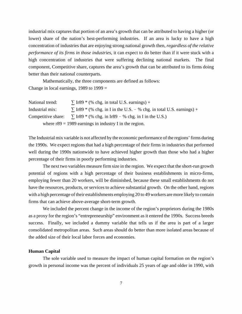
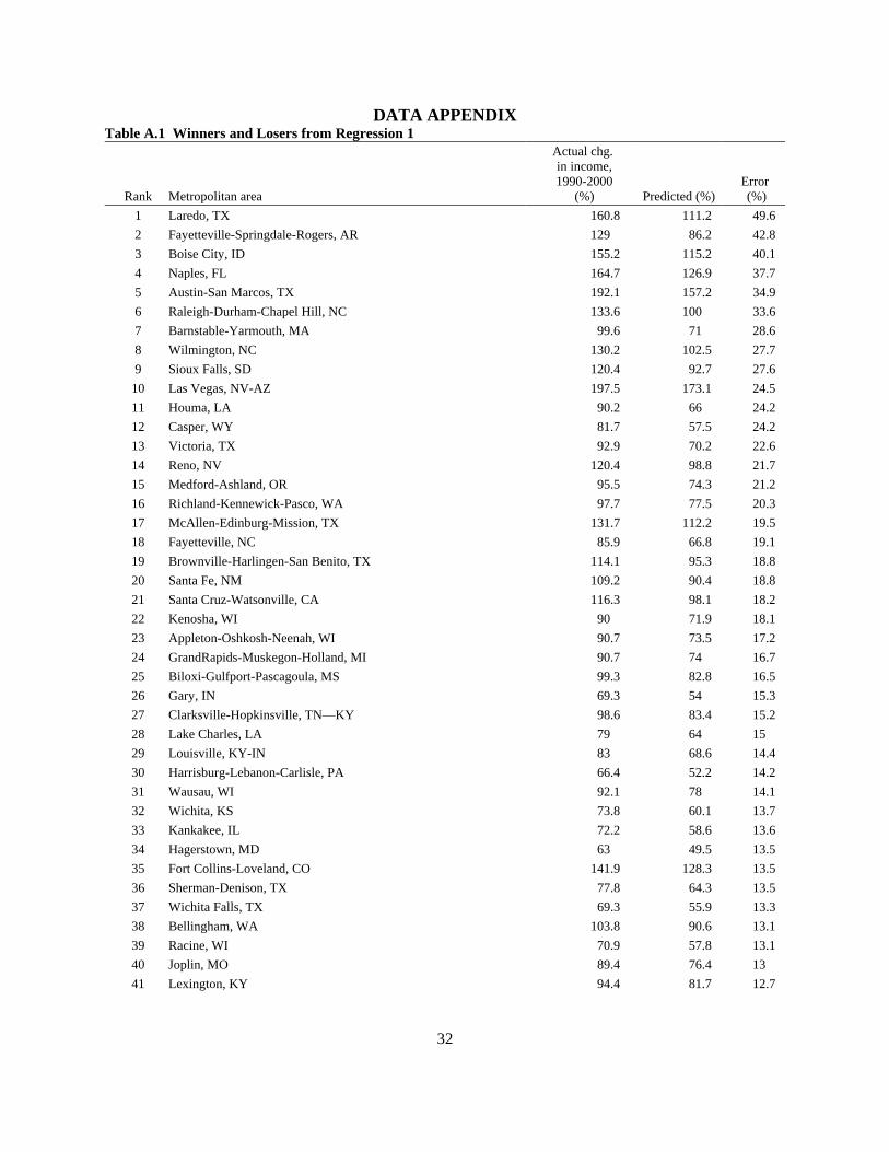
Winners and LosersTable A.1 in the appendix ranks all 267 metro areas in our analysis according the size of the

error term associated with the regression in Table 2. The way to interpret this error term is asfollows: whereas the model predicted personal income in Laredo, Texas, would increase by 111.2percent during the 1990s, personal income actually rose by 160.8 percent. In other words, Laredoexceeded the model’s forecast of its personal income growth by 49.6 percent. At the other end ofthe spectrum, personal income in El Paso, Texas was predicted to increase by 118.5 percent butgrew by only 86.0 percent.

The results are encouraging since metropolitan areas in similar environments can havestrikingly different error values, suggesting that unique public policy actions and economicdevelopment events or accidents may have made a difference. For example, even though El Paso,Texas, is the only other main border city in Texas besides Laredo, it did surprisingly poorly.Likewise, although Melbourne-Titusville-Palm Bay, Florida, performed well below expectations,Naples, Florida, strongly exceeded expectations.

Finally, the unique structure of the rankings below must be remembered. The top and lowestranked metro areas are nothing more than statistical outliers. They do not share any commonalityother than that they defied the model’s forecast. For example, personal income in Laredo grew by160.8 percent from 1989 to 1999. However, personal income in Provo–Orem, Utah, grew by astrong 146.9 percent, yet the city is ranked only 253th because the model predicted that it shouldhave grown by 165.0 percent. In fact, the rapidly expanding Provo–Orem area is ranked right belowDothan, Alabama, which grew by only 62.5 percent during the period (the model predicted thatpersonal income in the area would have grown by 80.3 percent).

The next step in the analysis is to attempt to uncover the reasons why some areas did farbetter or worse than expected.

11

AN EXPLORATORY ANALYSIS OF POSSIBLE PUBLIC POLICY IMPACTSSeveral previous studies suggest that public policy actions on the state and local levels may

have limited results, while others conclude that such actions do have positive benefits (Wassmer1994). Crihfield and Panggabean (1995) studied 282 metro areas from 1960 to 1982 and found that“public policies, and especially public-sector investments, played an insignificant role inmetropolitan growth and in convergence of per capital incomes” (p. 157). They concluded that“there is virtually no evidence that local or state infrastructure plays an important role in the growthof metropolitan economies” (p. 160). Similarly, Friedman (1995) could find no best practices forsmall firm formation. Still, after surveying 65 cities with populations of greater than 250,000 where71 major cultural buildings had been built in a short time span, Strom (2002) concluded thatspending on culture and the arts may help attract knowledge workers. Moreover, Johnson (2002),in his review of case studies, concluded that civic entrepreneurship where local governments createpartnerships and alliances with industry and universities can be the key to revival of distressed areas.An example is Tacoma, Washington, where access to broadband communication technology appearsto be spurring economic growth.

Disagreement exists regarding the importance of federal policies as well. Markusen andCarlson (1989) say federal policy is vital to any region’s sustainability. “If a city lacks the basicsfor economic viability, what does it have left except some type of massive support by the federalgovernment?” (Irving Baker, quoted in Kelley 1996, p. 36) But what if the federal government hasno specific urban policy? Bourne (1991) points out that the trend since the 1980s has been towardpolitical decentralization, fragmentation, deregulation of the private sector, and relocation offunctions and responsibilities from the public to the private sphere. This trend has not changed(National League of Cities 2003).

A TEST OF THE IMPORTANCE OF GOVERNMENTAL ACTIVITYAs a first step, a regression was run using the error term from the regression equation in

Table 2 as the dependent variable. The independent variables were proxies for changes in the levelof governmental activity within the area during the decade of the 1990s and for connections betweenlocal governments and the regional economy. Descriptive statistics are given in Table 3.

Quantifying the ability of government policy to affect the economic outcome of a region isdifficult. One of the major problems is that every state defines the powers and responsibilities oflocal governments differently, so policies that may appear to be the same across jurisdictions canbe very different in practice. Even within states, policies can appear to be identical, but in actualitybe very different in focus and intended outcomes. Yet, in a very general sense, public policy should

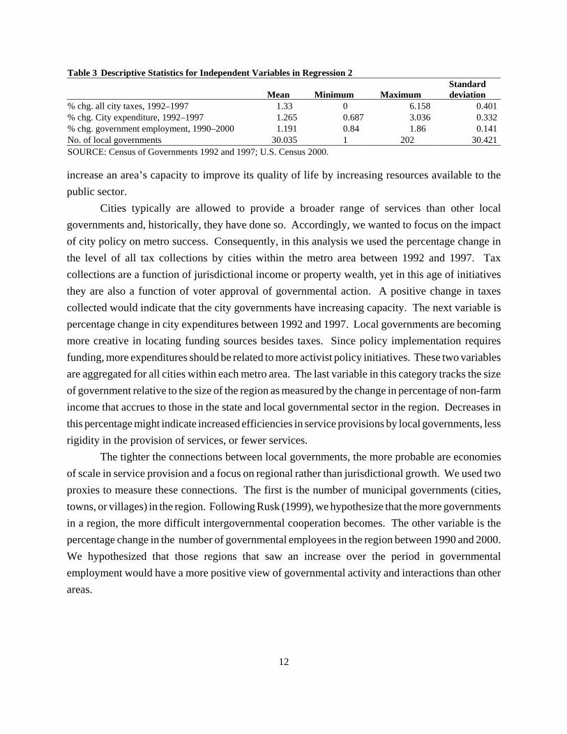
12

Table 3 Descriptive Statistics for Independent Variables in Regression 2

Mean Minimum MaximumStandarddeviation

% chg. all city taxes, 1992–1997 1.33 0 6.158 0.401% chg. City expenditure, 1992–1997 1.265 0.687 3.036 0.332% chg. government employment, 1990–2000 1.191 0.84 1.86 0.141No. of local governments 30.035 1 202 30.421SOURCE: Census of Governments 1992 and 1997; U.S. Census 2000.

increase an area’s capacity to improve its quality of life by increasing resources available to thepublic sector.

Cities typically are allowed to provide a broader range of services than other localgovernments and, historically, they have done so. Accordingly, we wanted to focus on the impactof city policy on metro success. Consequently, in this analysis we used the percentage change inthe level of all tax collections by cities within the metro area between 1992 and 1997. Taxcollections are a function of jurisdictional income or property wealth, yet in this age of initiativesthey are also a function of voter approval of governmental action. A positive change in taxescollected would indicate that the city governments have increasing capacity. The next variable ispercentage change in city expenditures between 1992 and 1997. Local governments are becomingmore creative in locating funding sources besides taxes. Since policy implementation requiresfunding, more expenditures should be related to more activist policy initiatives. These two variablesare aggregated for all cities within each metro area. The last variable in this category tracks the sizeof government relative to the size of the region as measured by the change in percentage of non-farmincome that accrues to those in the state and local governmental sector in the region. Decreases inthis percentage might indicate increased efficiencies in service provisions by local governments, lessrigidity in the provision of services, or fewer services.

The tighter the connections between local governments, the more probable are economiesof scale in service provision and a focus on regional rather than jurisdictional growth. We used twoproxies to measure these connections. The first is the number of municipal governments (cities,towns, or villages) in the region. Following Rusk (1999), we hypothesize that the more governmentsin a region, the more difficult intergovernmental cooperation becomes. The other variable is thepercentage change in the number of governmental employees in the region between 1990 and 2000.We hypothesized that those regions that saw an increase over the period in governmentalemployment would have a more positive view of governmental activity and interactions than otherareas.

13

Regression ResultsThe results are given in Table 4. The variables measuring change in the level of

governmental activity are all significant with the expected signs; however, only 17 percent ofvariation in the error term was explained by the regression. Nonetheless, the regression offers someevidence that governmental activity is related to regional performance in the 1990s even though itgives us no indication of what local governments did that added to the region’s success. The errorterm from regression 1, indicating the difference between predicted and actual income growth, wasboth positive and larger for the areas’ expenditures, indicating that these are areas that performedbetter than expected. Tax collections were positive but not significant. At the same time, for areasthat outperformed the forecast, employment in all governmental sectors increased significantly overthe 1990s. The more local governments in a region, the more likely a region was to haveoutperformed the forecast. This may reflect an intraregional migration of people and business fromhigh-tax, high-public-activity cities to low-cost, low-service-provision suburbs.

Table 4 Regression 2: Impact of Government on Error in Regression 1Dependent variable: Winner and loser status (error term from regression 1)

Changes in levels of governmental activityCoefficient Std. err. T-stat P>|t|

% chg. city expenditure, 1992 to 1997 0.087 0.025 3.56 0% chg. all city taxes, 1992 to 1997 0.025 0.02 1.256 0.21% chg. governmental employment,

1990 to 2000 0.269 0.052 5.196 0

No. of local governments 0.001.0.00

0 2.728 0.007

Constant !0.485 0.067 !7.186 0Observations 267Adj. R-square 0.174

CLUSTER ANALYSIS BASED ON CHANGES IN REGIONAL PERFORMANCEDURING THE 1990S

In this section we report on results obtained with a more exploratory technique called clusteranalysis. The technique is designed to reveal natural groupings (or clusters) within a data set thatwould otherwise not be apparent. It sorts the metro areas into groups sharing similar changes infiscal, social, or demographic characteristics during the 1990s. The analysis creates groups inwhich group members are as homogeneous as possible, with respect to the means of the variablesused in the analysis, while being as distinct as possible from members of other groups, again withrespect to the means. The number of clusters is arbitrary, and membership in a cluster can changewhen variables are added to or subtracted from the analysis, or when the number of clusters is

14

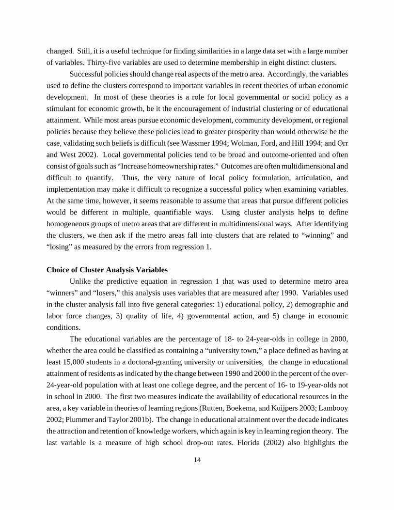
changed. Still, it is a useful technique for finding similarities in a large data set with a large numberof variables. Thirty-five variables are used to determine membership in eight distinct clusters.

Successful policies should change real aspects of the metro area. Accordingly, the variablesused to define the clusters correspond to important variables in recent theories of urban economicdevelopment. In most of these theories is a role for local governmental or social policy as astimulant for economic growth, be it the encouragement of industrial clustering or of educationalattainment. While most areas pursue economic development, community development, or regionalpolicies because they believe these policies lead to greater prosperity than would otherwise be thecase, validating such beliefs is difficult (see Wassmer 1994; Wolman, Ford, and Hill 1994; and Orrand West 2002). Local governmental policies tend to be broad and outcome-oriented and oftenconsist of goals such as “Increase homeownership rates.” Outcomes are often multidimensional anddifficult to quantify. Thus, the very nature of local policy formulation, articulation, andimplementation may make it difficult to recognize a successful policy when examining variables.At the same time, however, it seems reasonable to assume that areas that pursue different policieswould be different in multiple, quantifiable ways. Using cluster analysis helps to definehomogeneous groups of metro areas that are different in multidimensional ways. After identifyingthe clusters, we then ask if the metro areas fall into clusters that are related to “winning” and“losing” as measured by the errors from regression 1.

Choice of Cluster Analysis VariablesUnlike the predictive equation in regression 1 that was used to determine metro area

“winners” and “losers,” this analysis uses variables that are measured after 1990. Variables usedin the cluster analysis fall into five general categories: 1) educational policy, 2) demographic andlabor force changes, 3) quality of life, 4) governmental action, and 5) change in economicconditions.

The educational variables are the percentage of 18- to 24-year-olds in college in 2000,whether the area could be classified as containing a “university town,” a place defined as having atleast 15,000 students in a doctoral-granting university or universities, the change in educationalattainment of residents as indicated by the change between 1990 and 2000 in the percent of the over-24-year-old population with at least one college degree, and the percent of 16- to 19-year-olds notin school in 2000. The first two measures indicate the availability of educational resources in thearea, a key variable in theories of learning regions (Rutten, Boekema, and Kuijpers 2003; Lambooy2002; Plummer and Taylor 2001b). The change in educational attainment over the decade indicatesthe attraction and retention of knowledge workers, which again is key in learning region theory. Thelast variable is a measure of high school drop-out rates. Florida (2002) also highlights the

15

importance of education or human capital development in spurring growth, although in some casesit is an amenity that brings knowledge workers rather than a root cause of human capital formation.

Demographic and labor force changes within the metro areas are captured by eight variables.The change between 1990 and 2000 in the percentage of the population that is Hispanic and thechange over the same time period in the percent of the population that is African American areincluded. Minority population growth, particularly that of Asians and Hispanics, is related to strongpopulation growth in many of the nation’s metropolitan areas (Singer 2004; Berube 2003). Thepercentage change between 1990 and 2000 in the population is also included. Aspects of labordemand and supply are captured by the other six variables in this category. The tightness of thelabor force indicates strong labor demand and is measured by the percent of women with youngchildren in the labor force in 2000, the overall unemployment rate in 2000, the percentage changebetween 1990 and 2000 in employment, the metro poverty rate in 2000, and the percentage changein the poverty rate between 1990 and 2000.

The income-related quality of life variables are measured as changes from 1990 to 2000,while the crime-related quality of life variables are measured as changes from 1992 to 2000. Theincome-related variables are change in the median mortgage rate, change in median income, changein median income in the suburban part of the metro area, and change in the number of householdswith incomes above the 80th percentile of national income. The crime variables are change in theburglary rate and change in the murder rate. These variables reflect social stability as well as socialopportunity in the region. They are related to profit cycle theory, in which the life cycle of firmsdrives regional growth and decline (see Markusen 1985). They may also be related to communityasset building, a policy that links low-income and other residents to economic opportunity (Kazisand Miller 2001).

Many authors believe that the presence of public sector infrastructure and high levels ofgovernment spending are key to an area’s viability in this age of footloose industry (Markusen, Leeand DiGiovanna 1999). The extent of governmental activity in the area is measured by the numberof municipal governments, the percentage change between 1990 and 2000 in total governmentalemployment in the region, and if the area contains the state capital. Several proxies for changes inthe fiscal capacity and actions of city governments are used. These are changes between 1992 and1997 in state aid, property tax revenues, sales tax revenues, miscellaneous taxes, long term debt, andpublic expenditures in cities. Leaders in many municipalities often believe a change in the tax baseor increased expenditures on infrastructure or programs will lead to economic growth.

The last group of variables measure economic conditions and opportunities within the area.The percent change in export sales between 1993 and 1997 shows the region’s connection to theglobal economy. Two variables, change in Fortune 500 firm revenue between 1990 and 2000 and

16

the revenues of the Fortune 1000 firms (net of the Fortune 500 revenues) in 2000, indicate theregion’s dependence on large firms – important in theories of enterprise segmentation (Plummer andTaylor 2001a) and the previously mentioned product cycle theory. Changes in the manufacturingbase of the area are measured by the percentage changes in the location quotient of manufacturingbetween 1979 and 1999 and between 1989 and 1999. Changes in the overall productive capacityof a region are captured in the competitive shift variable which measures how an area’s firms aredoing relative to their national counterparts.

Table 5 shows the cluster definitions and the variable means. The names of the cities in eachcluster are given in Table A.2. The starred means are significantly different from the group mean(shown in the column labeled “Combined Metro Areas”), which is determined by takingsimultaneous 95 (%) confidence intervals for the mean of each group. An overview of groupcharacteristics is given below.

Group 1: Old economy places in slow decline (65 metro areas)As the industrial structures of these areas changed, these places seemed to lack the breadth

of resources to counteract private sector losses. These areas saw significantly less growth in Fortune500 firm revenue; fewer second-tier Fortune 1000 firms, and the smallest twenty-year trend in themanufacturing location quotient of all clusters. Falling median incomes, loss of high-incomepeople, and little immigration of minority groups characterize these areas. Included in this groupwere cities like Allentown, Pennsylvania; and Flint, Michigan.

Group 2: Private sector dependent places (79 metro areas)These areas lacked significant university facilities or state capitals. Not surprisingly, they

had significantly higher high school drop-out rates than other areas as a whole, and lowerpercentages of young adults in college. They had a metro poverty rate that was significantly higherthan that of all groups combined. Their industrial base was shrinking, as measured by the negativechange in Fortune 500 revenue between 1990 and 2000 and a significantly low amount of Fortune1000 firm revenue. When the private sector shrank, public sector institutions were not available tohelp buffer the impacts of the changed local economy. Jackson, Tennessee; and Fayetteville, NorthCarolina, are included in this group.

Group 3: Sprawling places (34 metro areas)These areas have the most fragmented local government, having on average 68.5

governments compared to overall group mean of 29.9. Median income change for both the metro

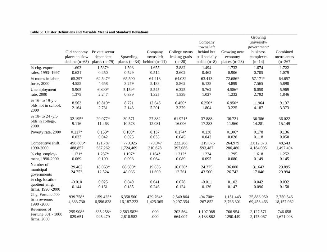
Table 5: Cluster Definitions and Variable Means and Standard Deviations

Old economyplaces in slowdecline (n=65)

Private sectordependent

places (n=79)Sprawling

places (n=34)

Companytowns left

behind (n=11)

College townsleaking grads

(n=28)

Companytowns leftbehind but

still sociallystable (n=8)

Growing neweconomy

places (n=28)

Growinguniversity/

government/business

complexes(n=14)

Combinedmetro areas

(n=267% chg. exportsales, 1993- 1997

1.6030.631

1.537*0.450

1.5080.529

1.6550.514

2.8822.602

1.4940.462

1.7320.906

1.6740.705

1.7221.079

% moms in laborforce, 2000

65.3974.555

62.547*4.658

65.5003.279

64.4185.188

64.0325.862

63.4136.138

72.686*4.899

57.171*7.565

64.6575.898

Unemploymentrate, 2000

5.9051.375

6.800*2.247

5.159*0.839

5.5451.325

6.3251.539

5.7621.027

4.586*1.232

6.0502.792

5.9691.846

% 16- to 19-yr.-olds not in school,2000

8.5632.164

10.819*2.731

8.7212.143

12.6455.201

6.450*3.279

6.250*1.804

6.950*3.225

11.9644.187

9.1373.373

% 18- to 24 -yr.-olds in college,2000

32.195*9.116

29.077*11.463

39.57110.573

27.88212.031

61.971*16.006

37.88817.283

36.72111.960

36.38614.281

36.02215.149

Poverty rate, 2000

0.117*0.033

0.153*0.042

0.109*0.025

0.1370.035

0.174*0.045

0.1300.043

0.106*0.028

0.1780.118

0.1360.050

Competitive shift,1990-2000

!498,803*488,857

121,787537,262

!770,9251,724,469

!70,047210,678

232,288397,086

!219,076593,487

264,979286,480

3,612,3734,184,005

48,5431,497,404

% chg. employ-ment, 1990-2000

1.131*0.069

1.287*0.109

1.197*0.098

1.164*0.064

1.312*0.089

1.2340.095

1.2950.080

1.6180.149

1.2520.145

Number ofmunicipalgovernments

29.46224.753

18.063*12.524

68.500*48.036

19.63611.690

16.036*12.761

24.37543.500

36.00026.742

31.64317.046

29.89529.994

% chg. locationquotient mfg.firms, 1990 -2000

-0.0100.144

0.0250.161

0.0400.185

0.0410.246

0.0780.124

-0.0110.136

0.1020.147

0.0420.096

0.0320.158

Chg. Fortune 500firm revenue, 1990 -2000

939.758*4,333.730

-159.425*6,596.828

6,358.50016,187.223

429.764*1,425.365

2,540.8649,297.354

-94.700*267.852

1,151.4433,766.301

25,883.05069,453.463

2,750.54618,157.962

Revenues ofFortune 501 - 1000firms, 2000

295.908*829.651

335.258*925.479

2,583.582*2,818.582

.000

.000202.564664.007

1,107.9883,133.862

766.9541290.449

2,127.5712,175.067

746.6581,671.993

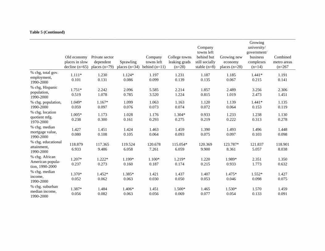
Table 5 (Continued)

Old economyplaces in slowdecline (n=65)

Private sectordependent

places (n=79)Sprawling

places (n=34)

Companytowns left

behind (n=11)

College townsleaking grads

(n=28)

Companytowns leftbehind but

still sociallystable (n=8)

Growing neweconomy

places (n=28)

Growinguniversity/

government/business

complexes(n=14)

Combinedmetro areas

(n=267% chg, total gov.employment, 1990-2000

1.111*0.101

1.2300.131

1.124*0.086

1.1970.099

1.2310.139

1.1870.135

1.1850.067

1.441*0.215

1.1910.141

% chg, Hispanicpopulation, 1990-2000

1.751*0.519

2.2421.078

2.0960.785

5.5853.520

2.2141.224

1.8570.815

2.4891.019

3.2562.473

2.3061.451

% chg. population,1990-2000

1.049*0.059

1.167*0.097

1.0990.076

1.0630.073

1.1630.074

1.1200.072

1.1390.064

1.441*0.153

1.1350.119

% chg. locationquotient mfg. 1970-2000

1.005*0.238

1.1730.300

1.0280.161

1.1760.293

1.304*0.275

0.9330.219

1.2330.222

1.2380.313

1.1300.278

% chg. medianmortgage value,1990-2000

1.4270.080

1.4510.108

1.4240.105

1.4630.064

1.4590.093

1.3900.075

1.4930.097

1.4960.103

1.4480.098

% chg. educationalattainment, 1990-2000

118.8796.933

117.3659.486

119.5246.058

120.6787.261

115.054*6.059

120.3699.900

123.787*8.361

121.8375.057

118.9018.038

% chg. AfricanAmerican popula-tion, 1990-2000

1.207*0.237

1.222*0.273

1.199*0.160

1.100*0.187

1.219*0.174

1.2200.215

1.989*0.933

2.3511.773

1.3500.632

% chg. medianincome, 1990-2000

1.370*0.052

1.452*0.062

1.385*0.063

1.4210.030

1.4370.050

1.4070.053

1.475*0.046

1.552*0.098

1.4270.075

% chg. suburbanmedian income,1990-2000

1.387*0.056

1.4840.082

1.406*0.063

1.4510.056

1.500*0.069

1.4650.077

1.530*0.054

1.5700.133

1.4590.091

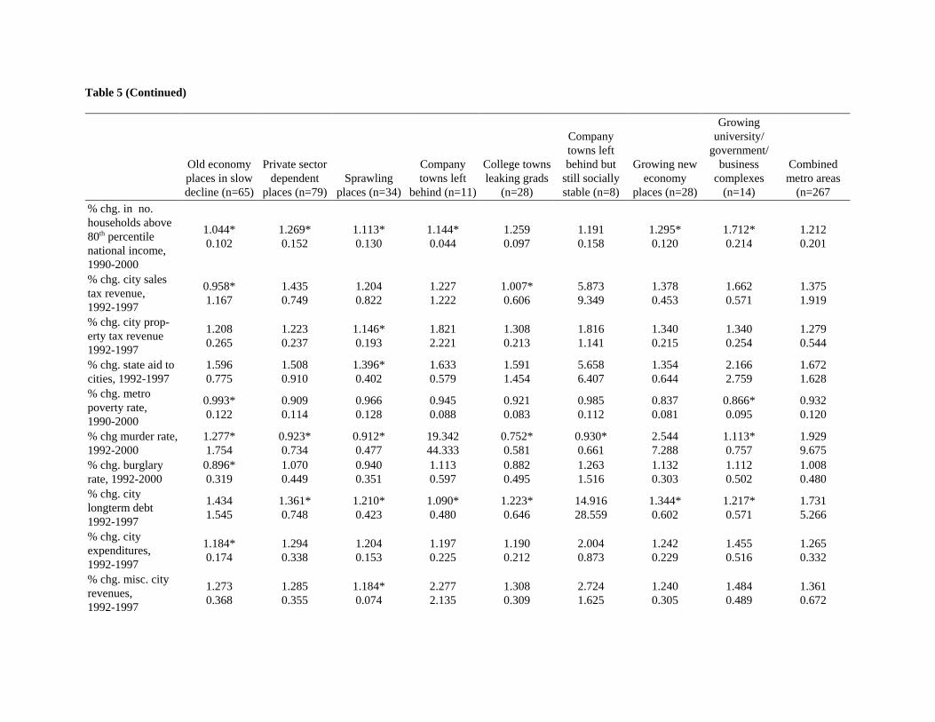
Table 5 (Continued)

Old economyplaces in slowdecline (n=65)

Private sectordependent

places (n=79)Sprawling

places (n=34)

Companytowns left

behind (n=11)

College townsleaking grads

(n=28)

Companytowns leftbehind but

still sociallystable (n=8)

Growing neweconomy

places (n=28)

Growinguniversity/

government/business

complexes(n=14)

Combinedmetro areas

(n=267% chg. in no.households above80th percentilenational income,1990-2000

1.044*0.102

1.269*0.152

1.113*0.130

1.144*0.044

1.2590.097

1.1910.158

1.295*0.120

1.712*0.214

1.2120.201

% chg. city salestax revenue, 1992-1997

0.958*1.167

1.4350.749

1.2040.822

1.2271.222

1.007*0.606

5.8739.349

1.3780.453

1.6620.571

1.3751.919

% chg. city prop-erty tax revenue1992-1997

1.2080.265

1.2230.237

1.146*0.193

1.8212.221

1.3080.213

1.8161.141

1.3400.215

1.3400.254

1.2790.544

% chg. state aid tocities, 1992-1997

1.5960.775

1.5080.910

1.396*0.402

1.6330.579

1.5911.454

5.6586.407

1.3540.644

2.1662.759

1.6721.628

% chg. metropoverty rate, 1990-2000

0.993*0.122

0.9090.114

0.9660.128

0.9450.088

0.9210.083

0.9850.112

0.8370.081

0.866*0.095

0.9320.120

% chg murder rate,1992-2000

1.277*1.754

0.923*0.734

0.912*0.477

19.34244.333

0.752*0.581

0.930*0.661

2.5447.288

1.113*0.757

1.9299.675

% chg. burglaryrate, 1992-2000

0.896*0.319

1.0700.449

0.9400.351

1.1130.597

0.8820.495

1.2631.516

1.1320.303

1.1120.502

1.0080.480

% chg. citylongterm debt1992-1997

1.4341.545

1.361*0.748

1.210*0.423

1.090*0.480

1.223*0.646

14.91628.559

1.344*0.602

1.217*0.571

1.7315.266

% chg. cityexpenditures, 1992-1997

1.184*0.174

1.2940.338

1.2040.153

1.1970.225

1.1900.212

2.0040.873

1.2420.229

1.4550.516

1.2650.332

% chg. misc. cityrevenues, 1992-1997

1.2730.368

1.2850.355

1.184*0.074

2.2772.135

1.3080.309

2.7241.625

1.2400.305

1.4840.489

1.3610.672

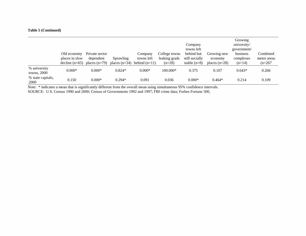
Table 5 (Continued)

Old economyplaces in slowdecline (n=65)

Private sectordependent

places (n=79)Sprawling

places (n=34)

Companytowns left

behind (n=11)

College townsleaking grads

(n=28)

Companytowns leftbehind but

still sociallystable (n=8)

Growing neweconomy

places (n=28)

Growinguniversity/

government/business

complexes(n=14)

Combinedmetro areas

(n=267% universitytowns, 2000 0.000* 0.000* 0.824* 0.000* 100.000* 0.375 0.107 0.643* 0.266

% state capitals,2000 0.150 0.000* 0.294* 0.091 0.036 0.000* 0.464* 0.214 0.109

Note: * indicates a mean that is significantly different from the overall mean using simultaneous 95% confidence intervals. SOURCE: U.S. Census 1990 and 2000; Census of Governments 1992 and 1997; FBI crime data; Forbes Fortune 500,

21

and the suburban places within the area was among the lowest. Employment grew little over thedecade, yet the unemployment rate in 2000 was among the lowest. Thirty of these places were eithera state capital or a university place, so changes in the private economy were buffered by the presenceof a large alternative employer. Kalamazoo, Michigan; and Burlington, Vermont, are among theseplaces.

Group 4: Company towns left behind (11 metro areas)These metro areas were primarily characterized by a loss of Fortune 500 firm revenue, low

employment growth over the decade of the 1990s, and no Fortune 1000 firms. Benton Harbor,Michigan; and Charleston, West Virginia, are included in this group.

Group 5: College places leaking graduates (28 metro areas)This group had the highest percentages of 18- to 24-year-olds in college (62 percent,

compared to the total average of 36.02 percent) and the lowest high school drop-out rate. Highemployment growth and compact local government also characterizes this group. Yet the 2000unemployment rate was significantly higher for this group than for all areas combined. Populationchange was similar to the overall mean, but the change in educational attainment for young adultswas below that of the overall mean. These are places of opportunity for the pursuit of highereducation but are not particularly strong magnets for college graduates. Terre Haute, Indiana; andChampaign-Urbana, Illinois, are among these areas.

Group 6: Company towns left behind but still socially stable (8 metro areas)This group saw Fortune 500 revenues shrinking over the decade. Yet, high school drop-out

rates were among the lowest, as were murder rates. All other variables were at the mean values forall areas. Lubbock, Texas, is in this group.

Group 7: Growing new economy places (28 metro areas)About half of these places were state capitals. These places had the highest percentage of

young mothers in the labor force, low poverty rates in 2000, and had relatively low high schooldrop-out rates. Labor was in demand in these areas. Moreover, the change in educationalattainment for young adults was the highest for this group. The Hispanic population grew at trend,but African-American population growth was above trend. All income variables were higher thanthe overall mean.

22

Group 8: Growing university/government/business complexes (14 metro areas)Something big was happening in these places. Government employment grew faster than

for other areas, many were university places or state capitals. Fewer young mothers were in theworkforce, yet median income grew significantly more than for the overall mean, and these areassaw the highest mean growth in higher-income families than other areas. They may be examplesof Bourne’s “few resource-based centers, typically small” that became sites of new mega-projects(Bourne 1991). WalMart headquarters’ home area, Fayetteville-Springdale-Rogers, Arkansas, isin this group, as is the heart of the research triangle, Raleigh-Durham-Chapel Hill, North Carolina.

DOES A RELATIONSHIP EXIST BETWEEN CLUSTER MEMBERSHIP ANDWINNING OR LOSING?

Now we turn to an exploration of the relationship between cluster membership and a regionbeing a “winner” or “loser” with respect to its change in personal income over the decade, asdetermined in regression 1. As a first step, an analysis of variance was performed using the errorfrom regression 1 as the dependent variable and cluster membership as the factor. The means areshown in Table 6. The F- statistic from the ANOVA was 9.472, with a p-value of 0.0001, whichindicates that at least one mean differed from the rest. A post hoc test was run to determine whichmeans were significantly different from one another. The last column in Table 6 shows which ofthe cluster means differ significantly. For example, the performance of areas in the “Old economyplaces in slow decline” cluster was significantly worse than those in the “Growing new economyplaces” and the “Growing university/government/business complexes,” with performance beingmeasured as the unexpected percentage change in personal income over the decade. A negativemean value in column 2 indicates that these areas tended to experience income growth below whatwould have been expected given the forecast equation. Positive values indicate that the cluster meanis weighted toward the “winners”—areas that did better than expected.

To examine the behavior of the most extreme winners and losers, two categorical variableswere created. These variables divide the 267 areas into three categories. The first category, “Ontrend,” contains the bulk of the metro areas and is defined as those whose forecasted growth wasclosest to their actual growth according to the regression. The second category, “Loser,” containsthose areas whose actual growth fell farthest below the forecasted growth. And the third category,“Winner,” contains those metro areas whose actual growth most exceeded the forecasted amount.The first categorical variable is determined by whether an area’s forecasted growth is two or morestandard deviations away from the mean (in Table A.1). In this variable, 254 metro areas are in the“On trend” category since they fall within two standard deviations of the mean, four are in the“Loser” category because they fell at least two standard deviations below the mean, and nine are in

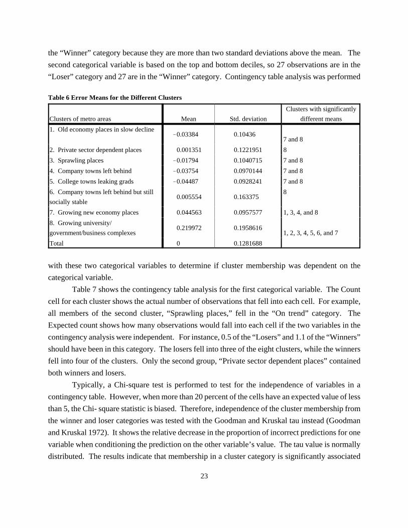
23

the “Winner” category because they are more than two standard deviations above the mean. Thesecond categorical variable is based on the top and bottom deciles, so 27 observations are in the“Loser” category and 27 are in the “Winner” category. Contingency table analysis was performed

Table 6 Error Means for the Different Clusters

Clusters of metro areas Mean Std. deviationClusters with significantly

different means1. Old economy places in slow decline

!0.03384 0.104367 and 8

2. Private sector dependent places 0.001351 0.1221951 83. Sprawling places !0.01794 0.1040715 7 and 84. Company towns left behind !0.03754 0.0970144 7 and 85. College towns leaking grads !0.04487 0.0928241 7 and 86. Company towns left behind but stillsocially stable

0.005554 0.1633758

7. Growing new economy places 0.044563 0.0957577 1, 3, 4, and 88. Growing university/government/business complexes

0.219972 0.19586161, 2, 3, 4, 5, 6, and 7

Total 0 0.1281688

with these two categorical variables to determine if cluster membership was dependent on thecategorical variable.

Table 7 shows the contingency table analysis for the first categorical variable. The Countcell for each cluster shows the actual number of observations that fell into each cell. For example,all members of the second cluster, “Sprawling places,” fell in the “On trend” category. TheExpected count shows how many observations would fall into each cell if the two variables in thecontingency analysis were independent. For instance, 0.5 of the “Losers” and 1.1 of the “Winners”should have been in this category. The losers fell into three of the eight clusters, while the winnersfell into four of the clusters. Only the second group, “Private sector dependent places” containedboth winners and losers.

Typically, a Chi-square test is performed to test for the independence of variables in acontingency table. However, when more than 20 percent of the cells have an expected value of lessthan 5, the Chi- square statistic is biased. Therefore, independence of the cluster membership fromthe winner and loser categories was tested with the Goodman and Kruskal tau instead (Goodmanand Kruskal 1972). It shows the relative decrease in the proportion of incorrect predictions for onevariable when conditioning the prediction on the other variable’s value. The tau value is normallydistributed. The results indicate that membership in a cluster category is significantly associated

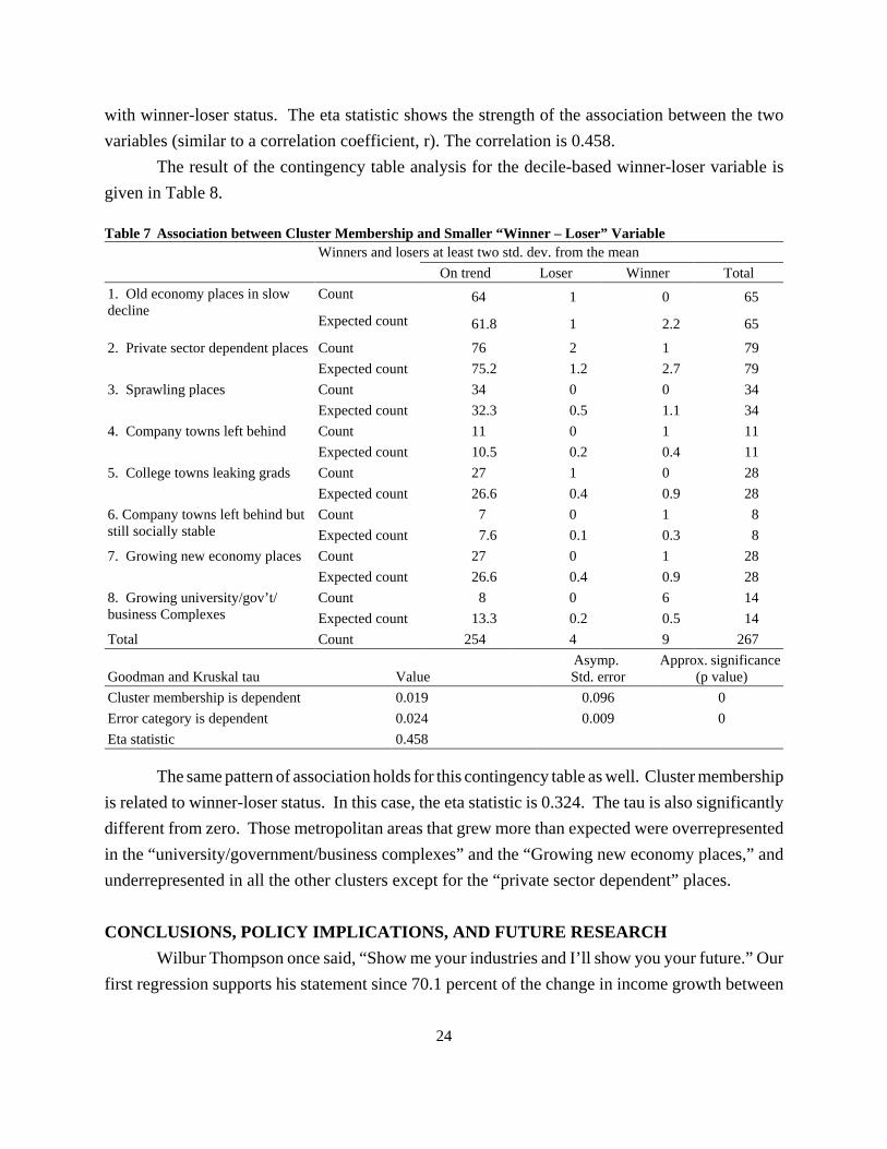
24

with winner-loser status. The eta statistic shows the strength of the association between the twovariables (similar to a correlation coefficient, r). The correlation is 0.458.

The result of the contingency table analysis for the decile-based winner-loser variable isgiven in Table 8.

Table 7 Association between Cluster Membership and Smaller “Winner – Loser” Variable Winners and losers at least two std. dev. from the mean On trend Loser Winner Total

1. Old economy places in slowdecline

Count 64 1 0 65

Expected count 61.8 1 2.2 65

2. Private sector dependent places Count 76 2 1 79Expected count 75.2 1.2 2.7 79

3. Sprawling places Count 34 0 0 34Expected count 32.3 0.5 1.1 34

4. Company towns left behind Count 11 0 1 11Expected count 10.5 0.2 0.4 11

5. College towns leaking grads Count 27 1 0 28Expected count 26.6 0.4 0.9 28

6. Company towns left behind butstill socially stable

Count 7 0 1 8Expected count 7.6 0.1 0.3 8

7. Growing new economy places Count 27 0 1 28Expected count 26.6 0.4 0.9 28

8. Growing university/gov’t/business Complexes

Count 8 0 6 14Expected count 13.3 0.2 0.5 14

Total Count 254 4 9 267

Goodman and Kruskal tau ValueAsymp. Std. error

Approx. significance (p value)

Cluster membership is dependent 0.019 0.096 0Error category is dependent 0.024 0.009 0Eta statistic 0.458

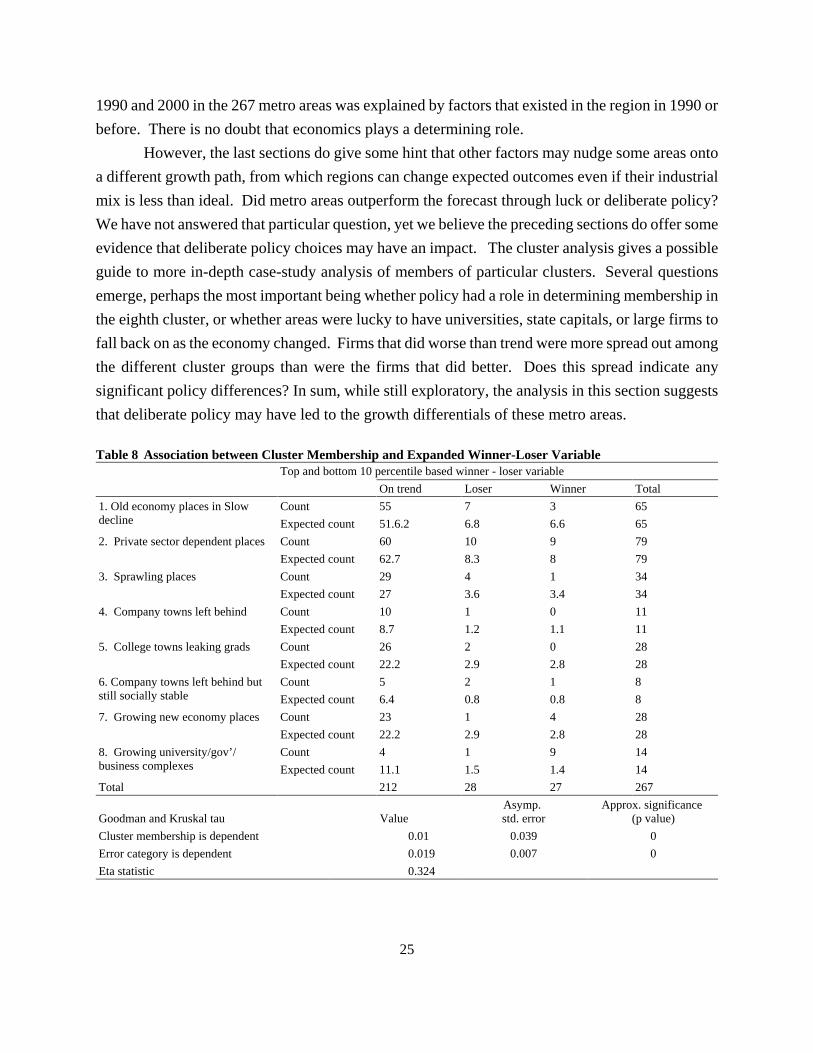
The same pattern of association holds for this contingency table as well. Cluster membershipis related to winner-loser status. In this case, the eta statistic is 0.324. The tau is also significantlydifferent from zero. Those metropolitan areas that grew more than expected were overrepresentedin the “university/government/business complexes” and the “Growing new economy places,” andunderrepresented in all the other clusters except for the “private sector dependent” places.

CONCLUSIONS, POLICY IMPLICATIONS, AND FUTURE RESEARCHWilbur Thompson once said, “Show me your industries and I’ll show you your future.” Our

first regression supports his statement since 70.1 percent of the change in income growth between

25

1990 and 2000 in the 267 metro areas was explained by factors that existed in the region in 1990 orbefore. There is no doubt that economics plays a determining role.

However, the last sections do give some hint that other factors may nudge some areas ontoa different growth path, from which regions can change expected outcomes even if their industrialmix is less than ideal. Did metro areas outperform the forecast through luck or deliberate policy?We have not answered that particular question, yet we believe the preceding sections do offer someevidence that deliberate policy choices may have an impact. The cluster analysis gives a possibleguide to more in-depth case-study analysis of members of particular clusters. Several questionsemerge, perhaps the most important being whether policy had a role in determining membership inthe eighth cluster, or whether areas were lucky to have universities, state capitals, or large firms tofall back on as the economy changed. Firms that did worse than trend were more spread out amongthe different cluster groups than were the firms that did better. Does this spread indicate anysignificant policy differences? In sum, while still exploratory, the analysis in this section suggeststhat deliberate policy may have led to the growth differentials of these metro areas.

Table 8 Association between Cluster Membership and Expanded Winner-Loser VariableTop and bottom 10 percentile based winner - loser variable

On trend Loser Winner Total1. Old economy places in Slowdecline

Count 55 7 3 65Expected count 51.6.2 6.8 6.6 65

2. Private sector dependent places Count 60 10 9 79Expected count 62.7 8.3 8 79

3. Sprawling places Count 29 4 1 34Expected count 27 3.6 3.4 34

4. Company towns left behind Count 10 1 0 11Expected count 8.7 1.2 1.1 11

5. College towns leaking grads Count 26 2 0 28Expected count 22.2 2.9 2.8 28

6. Company towns left behind butstill socially stable

Count 5 2 1 8Expected count 6.4 0.8 0.8 8

7. Growing new economy places Count 23 1 4 28Expected count 22.2 2.9 2.8 28

8. Growing university/gov’/business complexes

Count 4 1 9 14Expected count 11.1 1.5 1.4 14

Total 212 28 27 267

Goodman and Kruskal tau ValueAsymp. std. error

Approx. significance (p value)

Cluster membership is dependent 0.01 0.039 0Error category is dependent 0.019 0.007 0Eta statistic 0.324

26

REFERENCES

Anselin, Luc, Attila Varga, Zoltan J. Acs. 1997. “Entrepreneurship, Geographic Spillovers andUniversity Research: A Spatial Econometric Approach.” Working paper no. WP59.Cambridge, United Kingdom: Economic and Social Research Council, Centre for BusinessResearch,.

Barrow, Michael, and Mike, Hall. 1995. “The Impact of a Large Multinational Organization on aSmall Local Economy.” Regional Studies 29(7): 635–653.

Bee, Edward. 2003. “Knowledge Networks and Technical Invention in America’s MetropolitanAreas: A Paradigm for High-Technology Economic Development.” Economic DevelopmentQuarterly 17(2 ): 115–131.

Berube, Alan. 2003a. “Gaining but Losing Ground: Population Change in Large Cities and theirSuburbs.” In Redefining Urban and Suburban America: Evidence from Census 2000, BruceKatz and Robert Lang, eds. Washington, DC: Brookings Institution Press, pp. 33–50.

———. 2003b. “Racial and Ethnic Change in the Nation’s Largest Cities.” In Redefining Urban andSuburban America: Evidence from Census 2000. Bruce Katz and Robert Lang, eds.Washington, DC: Brookings Institution Press, pp. 137–154.

Bourne, L.S. 1991. “The Roepke Lecture in Economic Geography: Recycling Urban Systems andMetropolitan Areas: A Geographical Agenda for the 1990s and Beyond.” EconomicGeography 67(3): 185–209.

———. 1992. “Self-Fulfilling Prophecies? Decentralization, Inner City Decline, and the Qualityof Urban Life.” Journal of the American Planning Association. 58(4): 509–553.

Camagni, Roberto. 2002. “Cities and the Quality of Life: Problems and Prospects.” Review ofEconomic Conditions in Italy 0(1): 61–83.

Cook, Annabel Kirschner, and Donald M. Beck. 1991. “Metropolitan Dominance versusDecentralization in the Information Age.” Social Science Quarterly 72(2): 284–298.

27

Crihfield, John B., and Martin Panggabean. 1995. “Growth and Convergence in U.S. Cities.”Journal of Urban Economics 38(2): 138–165.

Ehrlich, Steven, and Joseph Gyourko. 2000. “Changes in the Scale and Size distribution of U.S.Metropolitan Areas during the Twentieth Century.” Urban Studies 37(7): 1063–1078.

Florida, Richard. 2002. The Rise of the Creative Class. New York: Basic Books.

Foust, Dean. 2003. “Blues for a Company Town.” Business Week, October 6, p. 56.

Friedman, Judith J. “The Effects of Industrial Structure and Resources upon the Distribution of Fast-Growing Small Firms among U.S. Urbanised Areas.” Urban Studies 32(6): 863–884.

Fulton, William, and Paul Shigley. 2001. “Small Towns Hang On.” Planning 67(4): 20–26.

Gabaix, Xavier. 1999. “Zipf’s Law and the Growth of Cities (in New Ideas on EconomicGrowth).”American Economic Review 89(2): 129–132.

Glaeser, Edward, and Jesse Shapiro. 2003a. “City Growth: Which Places Grew and Why.” InRedefining Urban and Suburban America: Evidence from Census 2000. Bruce Katz andRobert Lang, eds. Washington: Brookings Institution Press, pp. 13–32.

———. 2003b. “Urban Growth in the 1990s: Is City Living Back?” Journal of Regional Science43(1): 139–165.

Glaeser, Edward, Hedi Kallal, Jose Scheinkman, and Andrei Shleifer. 1992. “Growth in Cities.”Journal of Political Economy 100(6): 1126–1152.

Goodman, L.A., and W.H. Kruskal. 1972. “Measures of Association for Cross Classification IV:Simplification of Asymptotic Variances.” Journal of the American Statistical Association67: 415–421.

Gottlieb, Paul. 1995. “Residential Amenities, Firm Location, and Economic Development.” UrbanStudies 32(9): 1413–1436.

28

———. 2001. “Older Central Counties in the New Economy.” Working paper. Washington, DC:U.S. Department of Commerce, Economic Development Administration.

Johnson, James, Jr. 2002. “A Conceptual Model for Enhancing Community Competitiveness in theNew Economy.” Urban Affairs Review 378(6): 763–779.

Kazis, Richard, and Marc. S. Miller, eds. 2001. Knowledge and Urban Economic Development: AnEvolutionary Perspective on Low-Wage Workers in the New Economy. Washington, DC:Urban Institute Press.

Kelley, Chris. 1996. “In Search of New Life for Smaller Cities.” Public Management 78: 36–37.

Kirsch, Max H. 1998. In the Wake of the Giant: Multinational Restructuring and UnevenDevelopment in a New England Community. Albany: State University of New York Press.

Krugman, Paul. 1998. “Space: The Final Frontier.” Journal of Economic Perspectives 12(2):161–174.

Lambooy, Jan G. 2002. “Knowledge and Urban Economic Development: An EvolutionaryPerspective.” Urban Studies 39(5–6): 1019–1035.

Lovering, John. 1999. “Theory Led by Policy: The Inadequacies of the ‘New Regionalism.”

International Journal of Urban and Regional Research 23(2): 379–395.

Markusen, Ann. 1985. Profit Cycles, Oligopoly, and Regional Development. Cambridge, MA: MITPress.

Markusen, Ann, and Virginia Carlson. 1989. “Deindustrialization in the American Midwest: Causesand Responses.” In Deindustrialization and Regional Economic transformation: TheExperience of the United States, Lloyd Rodwin and Hidehiko Sazanami, eds. Boston: UnwinHyman, 29–59.

Markusen, Ann, Yong-Sook Lee, and Sean DiGiovanna, eds. 1999. Second Tier Cities: RapidGrowth Beyond the Metropolis. Minneapolis: University of Minnesota Press.

29

Martin, S.A., Richard McHugh, and S.R. Johnson. 1991. “The Influence of Location onProductivity: Manufacturing Technology in Rural and Urban Areas.” Discussion Paper 91-10. Washington, DC: U.S. Census Bureau, Center for Economic Studies.

Mayer, Henry, and Michael Greenberg. 2001. “Coming Back from Economic Despair: Case Studiesof Small- and Medium-Size American Cities.” Economic Development Quarterly 15(3):203–216.

Moore, Thomas. 1996. The Disposable Workforce: Worker Displacement and EmploymentInstability in America. New York: Aldine De Gruyter.

Moses, Nancy. 2001. “Have a Plan, And Make the Most of Arts and Culture.” Public Management83(11): 18–21.

National League of Cities. 2003. “Is the Federal–State–Local Partnership Being Dismantled?”Research Report, WHERE?

O hUallachain, Breandan. 1999. “Patent Places: Size Matters.” Journal of Regional Science 39(4):613–636.

Orr, Marian, and Darrell West. 2002. “Citizens’ Views on Urban Revitalization: The Case ofProvidence, Rhode Island.” Urban Affairs Review 37(3): 397–419.

Pack, Janet Rothenberg. 2002. Growth and Convergence in Metropolitan America. Washington,DC: Brookings Institution Press.

Palmer, Bryan D. 1994. Goodyear Invades the Backcountry: The Corporate Takeover of a RuralTown. New York: Monthly Review Press.

Plummer, Paul, and Mike Taylor. 2001. “Theories of Local Economic Growth (Part 1): Concepts,Models, and Measurement.” Environment and Planning A. 33: 219–236.

———. 2001. “Theories of Local Economic Growth (Part 2): Model Specification and EmpiricalValidation. Environment and Planning A. 33: 385–398.

30

Porter, Michael E. 2000. “Location, Competition, and Economic Development: Local Clusters ina Global Economy.” Economic Development Quarterly 4(1): 15–30.

———. 2003. “The Economic Performance of Regions.” Regional Studies 37(6–7): 549–578.

Raymond, Richard, and Thomas Pascarella. 1987. “Local Economic Development Programs andSmall City Growth in Northeastern Ohio, 1970–1980.” In Structural Change in an UrbanIndustrial Region. David McKee and Richard Bennett, eds. New York: Praeger, pp. XX

Rusk, David. 1999. Inside Game, Outside Game. Washington, DC: Brookings Institution Press.

Rutten, Roel, Frans Boekema, and Elsa Kuijpers. 2003. “Economic Geography of Higher Education:Knowledge Infrastructure and Learning Regions.” London and New York: Routledge.

Shilton, Leon, and Craig Stanley. 1999. “Spatial Patterns of Headquarters.” Journal of Real EstateResearch 17(3): 341–364.

Siegel, Beth, and Andy Waxman. 2001. “Third Tier Cities: Adjusting to the New Economy.”Reviews of Economic Development Literature and Practice no. 6. U.S. EconomicDevelopment Administration,.

Singer, Audrey. 2004. “The Rise of New Immigrant Gateways.” Brookings Institution, February.

Smith, Eldon D. 1990. “Economic Stability and Economic Growth in Rural Communities:Dimensions Relevant to Local Employment Creation Strategy,” Growth and Change 21(4):3–18.

Strom, Elizabeth. 2002. “Converting Pork into Porcelain. Cultural Institutions and DowntownDevelopment.” Urban Affairs Review 38(1): 3–21.

Teaford, Jon. 1994. Cities of the Heartland: The Rise and Fall of the Industrial Midwest.Bloomington: Indiana University Press.

31

U.S. Conference of Mayors. 2004. U.S. Metro Economies Special Report: Employment Update forthe State of Michigan, Types of Jobs Lost and Gained, 2001–2006. PUBLISHER?LOCATION?

U.S. Department of Housing and Urban Development. 1999. Now is the Time: Places Left Behindin the New Economy. http://www.hud.gov/library/bookshelf18/pressrel/leftbehind/menu.html.

Wassmer, Robert. 1994. “Can Local Incentives Alter a Metropolitan City’s EconomicDevelopment?” Urban Studies 31(8): 1251–1278.

Watts, H.D., and J.D. Kirkham. 1999. “Plant Closures by Multi-Locational Firms: A ComparativePerspective.” Regional Studies 33(5): 413–424.

Wojan, Timothy R., and Glen C. Pulver. 1995. “Location Patterns of High Growth Industries inRural Counties.” Growth and Change 26(1): 3–22.

Wolman, Harold L, Coit Cook Ford III, and Edward Hill. 1994. “Evaluating the Success of UrbanSuccess Stories” Urban Studies 31(6): 835–850.

Zelinsky, Wilbur. 1962. “Has American Industry Been Decentralizing? The Evidence for the1939–1954 Period.” Economic Geography 38(3): 251–269.

32

DATA APPENDIXTable A.1 Winners and Losers from Regression 1

Rank Metropolitan area

Actual chg. in income,1990-2000

(%) Predicted (%)Error (%)

1 Laredo, TX 160.8 111.2 49.62 Fayetteville-Springdale-Rogers, AR 129 86.2 42.83 Boise City, ID 155.2 115.2 40.14 Naples, FL 164.7 126.9 37.75 Austin-San Marcos, TX 192.1 157.2 34.96 Raleigh-Durham-Chapel Hill, NC 133.6 100 33.67 Barnstable-Yarmouth, MA 99.6 71 28.68 Wilmington, NC 130.2 102.5 27.79 Sioux Falls, SD 120.4 92.7 27.6

10 Las Vegas, NV-AZ 197.5 173.1 24.511 Houma, LA 90.2 66 24.212 Casper, WY 81.7 57.5 24.213 Victoria, TX 92.9 70.2 22.614 Reno, NV 120.4 98.8 21.715 Medford-Ashland, OR 95.5 74.3 21.216 Richland-Kennewick-Pasco, WA 97.7 77.5 20.317 McAllen-Edinburg-Mission, TX 131.7 112.2 19.518 Fayetteville, NC 85.9 66.8 19.119 Brownville-Harlingen-San Benito, TX 114.1 95.3 18.820 Santa Fe, NM 109.2 90.4 18.821 Santa Cruz-Watsonville, CA 116.3 98.1 18.222 Kenosha, WI 90 71.9 18.123 Appleton-Oshkosh-Neenah, WI 90.7 73.5 17.224 GrandRapids-Muskegon-Holland, MI 90.7 74 16.725 Biloxi-Gulfport-Pascagoula, MS 99.3 82.8 16.526 Gary, IN 69.3 54 15.327 Clarksville-Hopkinsville, TN—KY 98.6 83.4 15.228 Lake Charles, LA 79 64 1529 Louisville, KY-IN 83 68.6 14.430 Harrisburg-Lebanon-Carlisle, PA 66.4 52.2 14.231 Wausau, WI 92.1 78 14.132 Wichita, KS 73.8 60.1 13.733 Kankakee, IL 72.2 58.6 13.634 Hagerstown, MD 63 49.5 13.535 Fort Collins-Loveland, CO 141.9 128.3 13.536 Sherman-Denison, TX 77.8 64.3 13.537 Wichita Falls, TX 69.3 55.9 13.338 Bellingham, WA 103.8 90.6 13.139 Racine, WI 70.9 57.8 13.140 Joplin, MO 89.4 76.4 1341 Lexington, KY 94.4 81.7 12.7

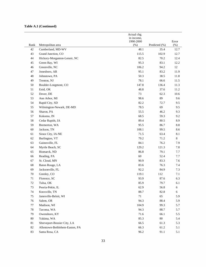
Table A.1 (Continued)

Rank Metropolitan area

Actual chg. in income,1990-2000

(%) Predicted (%)Error (%)

33

42 Cumberland, MD-WV 48.1 35.4 12.743 Grand Junction, CO 115.5 102.9 12.744 Hickory-Morganton-Lenoir, NC 82.5 70.2 12.445 Green Bay, WI 95.3 83.1 12.246 Greenville, NC 106.2 94.2 1247 Jonesboro, AR 95.1 83.2 11.948 Johnstown, PA 50.3 38.5 11.849 Trenton, NJ 78.1 66.6 11.550 Boulder-Longmont, CO 147.8 136.4 11.351 Enid, OK 48.8 37.6 11.252 Dover, DE 73 62.3 10.653 Ann Arbor, MI 98.6 89 9.654 Rapid City, SD 82.2 72.7 9.555 Wilmington-Newark, DE-MD 78.5 69 9.556 Sharon, PA 55.5 46.2 9.357 Kokomo, IN 68.5 59.3 9.258 Cedar Rapids, IA 89.4 80.5 8.959 Bremerton, WA 95.5 86.7 8.860 Jackson, TN 108.1 99.5 8.661 Sioux City, IA-NE 71.5 63.4 8.162 Burlington, VT 79.2 71.2 863 Gainesville, FL 84.1 76.2 7.964 Myrtle Beach, SC 129.2 121.3 7.865 Bismarck, ND 86.8 79.1 7.766 Reading, PA 60 52.4 7.767 St. Cloud, MN 90.9 83.3 7.668 Baton Rouge, LA 83.6 76.3 7.469 Jacksonville, FL 92.2 84.9 7.370 Greeley, CO 119.1 112 7.171 Florence, SC 93.9 87.6 6.372 Tulsa, OK 85.9 79.7 6.173 Peoria-Pekin, IL 62.9 56.8 674 Knoxville, TN 88.7 82.8 675 Janesville-Beloit, WI 71 65 5.976 Salem, OR 94.3 88.4 5.977 Madison, WI 104.9 99.3 5.778 Tacoma, WA 94.3 88.7 5.779 Owensboro, KY 71.6 66.1 5.580 Yakima, WA 85.3 80 5.481 Shreveport-Bossier City, LA 66.5 61.3 5.382 Allentown-Bethlehem-Easton, PA 66.3 61.2 5.183 Santa Rosa, CA 96.2 91.1 5.1

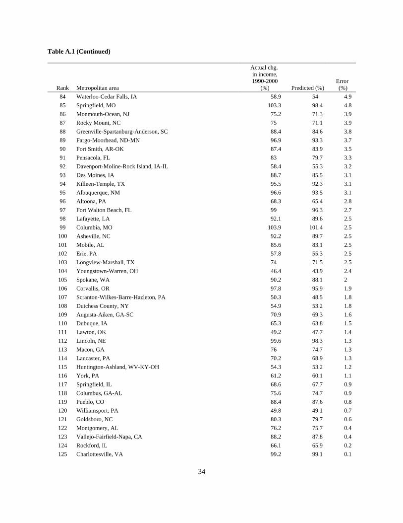
Table A.1 (Continued)

Rank Metropolitan area

Actual chg. in income,1990-2000

(%) Predicted (%)Error (%)

34

84 Waterloo-Cedar Falls, IA 58.9 54 4.985 Springfield, MO 103.3 98.4 4.886 Monmouth-Ocean, NJ 75.2 71.3 3.987 Rocky Mount, NC 75 71.1 3.988 Greenville-Spartanburg-Anderson, SC 88.4 84.6 3.889 Fargo-Moorhead, ND-MN 96.9 93.3 3.790 Fort Smith, AR-OK 87.4 83.9 3.591 Pensacola, FL 83 79.7 3.392 Davenport-Moline-Rock Island, IA-IL 58.4 55.3 3.293 Des Moines, IA 88.7 85.5 3.194 Killeen-Temple, TX 95.5 92.3 3.195 Albuquerque, NM 96.6 93.5 3.196 Altoona, PA 68.3 65.4 2.897 Fort Walton Beach, FL 99 96.3 2.798 Lafayette, LA 92.1 89.6 2.599 Columbia, MO 103.9 101.4 2.5100 Asheville, NC 92.2 89.7 2.5101 Mobile, AL 85.6 83.1 2.5102 Erie, PA 57.8 55.3 2.5103 Longview-Marshall, TX 74 71.5 2.5104 Youngstown-Warren, OH 46.4 43.9 2.4105 Spokane, WA 90.2 88.1 2106 Corvallis, OR 97.8 95.9 1.9107 Scranton-Wilkes-Barre-Hazleton, PA 50.3 48.5 1.8108 Dutchess County, NY 54.9 53.2 1.8109 Augusta-Aiken, GA-SC 70.9 69.3 1.6110 Dubuque, IA 65.3 63.8 1.5111 Lawton, OK 49.2 47.7 1.4112 Lincoln, NE 99.6 98.3 1.3113 Macon, GA 76 74.7 1.3114 Lancaster, PA 70.2 68.9 1.3115 Huntington-Ashland, WV-KY-OH 54.3 53.2 1.2116 York, PA 61.2 60.1 1.1117 Springfield, IL 68.6 67.7 0.9118 Columbus, GA-AL 75.6 74.7 0.9119 Pueblo, CO 88.4 87.6 0.8120 Williamsport, PA 49.8 49.1 0.7121 Goldsboro, NC 80.3 79.7 0.6122 Montgomery, AL 76.2 75.7 0.4123 Vallejo-Fairfield-Napa, CA 88.2 87.8 0.4124 Rockford, IL 66.1 65.9 0.2125 Charlottesville, VA 99.2 99.1 0.1

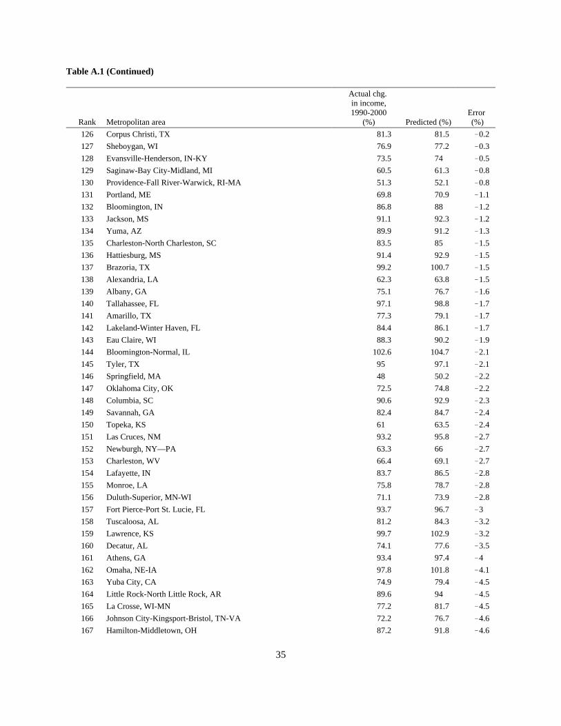
Table A.1 (Continued)

Rank Metropolitan area

Actual chg. in income,1990-2000

(%) Predicted (%)Error (%)

35

126 Corpus Christi, TX 81.3 81.5 !0.2127 Sheboygan, WI 76.9 77.2 !0.3128 Evansville-Henderson, IN-KY 73.5 74 !0.5129 Saginaw-Bay City-Midland, MI 60.5 61.3 !0.8130 Providence-Fall River-Warwick, RI-MA 51.3 52.1 !0.8131 Portland, ME 69.8 70.9 !1.1132 Bloomington, IN 86.8 88 !1.2133 Jackson, MS 91.1 92.3 !1.2134 Yuma, AZ 89.9 91.2 !1.3135 Charleston-North Charleston, SC 83.5 85 !1.5136 Hattiesburg, MS 91.4 92.9 !1.5137 Brazoria, TX 99.2 100.7 !1.5138 Alexandria, LA 62.3 63.8 !1.5139 Albany, GA 75.1 76.7 !1.6140 Tallahassee, FL 97.1 98.8 !1.7141 Amarillo, TX 77.3 79.1 !1.7142 Lakeland-Winter Haven, FL 84.4 86.1 !1.7143 Eau Claire, WI 88.3 90.2 !1.9144 Bloomington-Normal, IL 102.6 104.7 !2.1145 Tyler, TX 95 97.1 !2.1146 Springfield, MA 48 50.2 !2.2147 Oklahoma City, OK 72.5 74.8 !2.2148 Columbia, SC 90.6 92.9 !2.3149 Savannah, GA 82.4 84.7 !2.4150 Topeka, KS 61 63.5 !2.4151 Las Cruces, NM 93.2 95.8 !2.7152 Newburgh, NY—PA 63.3 66 !2.7153 Charleston, WV 66.4 69.1 !2.7154 Lafayette, IN 83.7 86.5 !2.8155 Monroe, LA 75.8 78.7 !2.8156 Duluth-Superior, MN-WI 71.1 73.9 !2.8157 Fort Pierce-Port St. Lucie, FL 93.7 96.7 !3158 Tuscaloosa, AL 81.2 84.3 !3.2159 Lawrence, KS 99.7 102.9 !3.2160 Decatur, AL 74.1 77.6 !3.5161 Athens, GA 93.4 97.4 !4162 Omaha, NE-IA 97.8 101.8 !4.1163 Yuba City, CA 74.9 79.4 !4.5164 Little Rock-North Little Rock, AR 89.6 94 !4.5165 La Crosse, WI-MN 77.2 81.7 !4.5166 Johnson City-Kingsport-Bristol, TN-VA 72.2 76.7 !4.6167 Hamilton-Middletown, OH 87.2 91.8 !4.6

Table A.1 (Continued)

Rank Metropolitan area

Actual chg. in income,1990-2000

(%) Predicted (%)Error (%)

36

168 Elmira, NY 53.3 58 !4.7169 Eugene-Springfield, OR 84.5 89.4 !4.8170 Olympia, WA 104.5 109.4 !4.9171 Terre Haute, IN 59.7 64.7 !5172 Decatur, IL 54.3 59.3 !5173 Birmingham, AL 83.6 88.7 !5.1174 Beaumont--Port Arthur, TX 65.8 71 !5.2175 Parkersburg-Marietta, WV—OH 58.2 63.5 !5.2176 Lubbock, TX 77.1 82.4 !5.3177 Bangor, ME 52.5 58 !5.5178 Elkhart-Goshen, IN 80 85.6 !5.6179 Danville, VA 49 54.7 !5.7180 Fort Wayne, IN 68.8 74.7 !5.9181 Texarkana, TX-Texarkana, AR 64.8 70.9 !6.1182 Lewiston-Auburn, ME 46.2 52.4 !6.1183 Wheeling, WV-OH 48.3 54.5 !6.1184 Ocala, FL 103.9 110.5 !6.6185 Rochester, MN 98.3 105 !6.7186 Pine Bluff, AR 47.8 54.8 !6.9187 Lima, OH 56 63.1 !7.1188 Visalia-Tulare-Porterville, CA 77 84.2 !7.2189 Chattanooga, TN-GA 78 85.2 !7.3190 Nashville, TN 113.2 120.6 !7.4191 Sarasota-Bradenton, FL 80.8 88.4 !7.5192 Richmond-Petersburg, VA 74.3 81.9 !7.6193 Sumter, SC 79.7 87.3 !7.6194 Roanoke, VA 67 74.9 !7.8195 Albany-Schenectady-Troy, NY 57.7 65.7 !8196 Flagstaff, AZ—UT 106.3 114.5 !8.2197 Jamestown, NY 43.2 51.5 !8.3198 Colorado Springs, CO 118.3 126.9 !8.6199 Dayton-Springfield, OH 56.6 65.3 !8.7200 Missoula, MT 99.9 108.8 !8.9201 San Angelo, TX 69.2 78.1 !8.9202 Santa Barbara-Santa Maria-Lompoc, CA 59.4 68.5 !9.1203 Muncie, IN 57.9 67.2 !9.2204 Fresno, CA 77.2 86.5 !9.3205 Florence, AL 61.6 70.9 !9.3206 Redding, CA 72.9 82.3 !9.4207 Akron, OH 69.8 79.3 !9.4208 Tucson, AZ 92.7 102.1 !9.5209 Daytona Beach, FL 80.6 90.1 !9.5

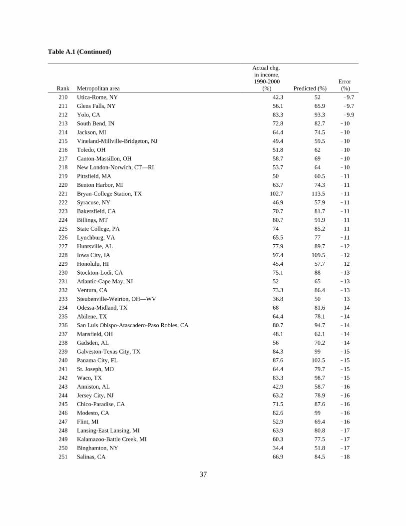
Table A.1 (Continued)

Rank Metropolitan area

Actual chg. in income,1990-2000

(%) Predicted (%)Error (%)

37

210 Utica-Rome, NY 42.3 52 !9.7211 Glens Falls, NY 56.1 65.9 !9.7212 Yolo, CA 83.3 93.3 !9.9213 South Bend, IN 72.8 82.7 !10214 Jackson, MI 64.4 74.5 !10215 Vineland-Millville-Bridgeton, NJ 49.4 59.5 !10216 Toledo, OH 51.8 62 !10217 Canton-Massillon, OH 58.7 69 !10218 New London-Norwich, CT—RI 53.7 64 !10219 Pittsfield, MA 50 60.5 !11220 Benton Harbor, MI 63.7 74.3 !11221 Bryan-College Station, TX 102.7 113.5 !11222 Syracuse, NY 46.9 57.9 !11223 Bakersfield, CA 70.7 81.7 !11224 Billings, MT 80.7 91.9 !11225 State College, PA 74 85.2 !11226 Lynchburg, VA 65.5 77 !11227 Huntsville, AL 77.9 89.7 !12228 Iowa City, IA 97.4 109.5 !12229 Honolulu, HI 45.4 57.7 !12230 Stockton-Lodi, CA 75.1 88 !13231 Atlantic-Cape May, NJ 52 65 !13232 Ventura, CA 73.3 86.4 !13233 Steubenville-Weirton, OH—WV 36.8 50 !13234 Odessa-Midland, TX 68 81.6 !14235 Abilene, TX 64.4 78.1 !14236 San Luis Obispo-Atascadero-Paso Robles, CA 80.7 94.7 !14237 Mansfield, OH 48.1 62.1 !14238 Gadsden, AL 56 70.2 !14239 Galveston-Texas City, TX 84.3 99 !15240 Panama City, FL 87.6 102.5 !15241 St. Joseph, MO 64.4 79.7 !15242 Waco, TX 83.3 98.7 !15243 Anniston, AL 42.9 58.7 !16244 Jersey City, NJ 63.2 78.9 !16245 Chico-Paradise, CA 71.5 87.6 !16246 Modesto, CA 82.6 99 !16247 Flint, MI 52.9 69.4 !16248 Lansing-East Lansing, MI 63.9 80.8 !17249 Kalamazoo-Battle Creek, MI 60.3 77.5 !17250 Binghamton, NY 34.4 51.8 !17251 Salinas, CA 66.9 84.5 !18

Table A.1 (Continued)

Rank Metropolitan area

Actual chg. in income,1990-2000

(%) Predicted (%)Error (%)

38

252 Dothan, AL 62.5 80.3 !18253 Provo-Orem, UT 146.9 165 !18254 Anchorage, AK 65.1 83.4 !18255 Cheyenne, WY 80.2 99.8 !20256 Pocatello, ID 81.2 100.9 !20257 Champaign-Urbana, IL 64 84.3 !20258 Grand Forks, ND—MN 56 76.7 !21259 Fort Myers-Cape Coral, FL 83.7 104.4 !21260 Jacksonville, NC 64 85.3 !21261 West Palm Beach-Boca Raton, FL 98.5 120.8 !22262 Merced, CA 61 84.1 !23263 Great Falls, MT 56.2 79.7 !24264 Melbourne-Titusville-Palm Bay, FL 75.4 101.3 !26265 Punta Gorda, FL 86.7 116.8 !30266 Auburn-Opelika, AL 80.9 112 !31267 El Paso, TX 86 118.5 !32

39

Table A.2 Metro Areas in Each Cluster

GROUP 1: Old economy places in slow decline (n=65)Allentown-Bethlehem-Easton, PA Anniston, AL Atlantic-Cape May, NJ Bangor, ME Billings, MT Binghamton, NY Canton-Massillon, OH Casper, WY Charleston-North Charleston, SC Cumberland, MD-WV Danville, VA Davenport-Moline-Rock Island, IA-IL Decatur, IL Dothan, AL Dutchess County, NY Elmira, NY Enid, OK Erie, PA Evansville-Henderson, IN-KY Flint, MI Fort Wayne, IN Gary, IN Glens Falls, NY Great Falls, MT Hagerstown, MD Huntington-Ashland, WV-KY-OH Jackson, MI Jamestown, NY Jersey City, NJ Johnson City-Kingsport-Bristol, TN-VA Johnstown, PA Lancaster, PA Lewiston-Auburn, ME Lima, OH Lynchburg, VA Macon, GA Mansfield, OH Melbourne-Titusville-Palm Bay, FL New London-Norwich, CT-RI Newburgh, NY-PA Odessa-Midland, TX Parkersburg-Marietta, WV-OH Peoria-Pekin, IL Pittsfield, MA Portland, ME Racine, WI Reading, PA Redding, CA Roanoke, VA Saginaw-Bay City-Midland, MI San Angelo, TX Santa Cruz-Watsonville, CA Sharon, PA South Bend, IN Steubenville-Weirton, OH-WV Texarkana, TX-Texarkana, AR Trenton, NJ

Utica-Rome, NY Vallejo-Fairfield-Napa, CA Ventura, CA Vineland-Millville-Bridgeton, NJ Wheeling, WV-OH Wichita Falls, TX Williamsport, PA York, PA

GROUP 2: Private sector dependent places (n=79)Abilene, TX Albany, GA Alexandria, LA Amarillo, TX Asheville, NC Auburn-Opelika, AL Bakersfield, CA Beaumont-Port Arthur, TX Bellingham, WA Biloxi-Gulfport-Pascagoula, MS Brazoria, TX Bremerton, WA Chattanooga, TN-GA Chico-Paradise, CA Clarksville-Hopkinsville, TN-KY Colorado Springs, CO Columbus, GA-AL Corpus Christi, TX Daytona Beach, FL Fayetteville, NC Fort Myers-Cape Coral, FL Fort Pierce-Port St. Lucie, FL Fort Smith, AR-OK Fort Walton Beach, FL Fresno, CA Galveston-Texas City, TX Goldsboro, NC Grand Junction, CO Hamilton-Middletown, OH Hattiesburg, MS Houma, LA Jackson, TN Joplin, MO Kankakee, IL Killeen-Temple, TX Kokomo, IN Lake Charles, LA Lakeland-Winter Haven, FL Lawton, OK Longview-Marshall, TX Medford-Ashland, OR Merced, CA Missoula, MT Mobile, AL Modesto, CA Monroe, LA Myrtle Beach, SC Ocala, FL

Table A.2 (Continued)

40

Owensboro, KY Panama City, FL Pensacola, FL Pine Bluff, AR Pueblo, CO Punta Gorda, FL Rapid City, SD Reno, NV Richland-Kennewick-Pasco, WA Rockford, IL Salinas, CA Santa Rosa, CA Sarasota-Bradenton, FL Savannah, GA Sherman-Denison, TX Shreveport-Bossier City, LA Sioux City, IA-NE Spokane, WA Springfield, MO St. Joseph, MO Stockton-Lodi, CA Sumter, SC Tacoma, WA Tyler, TX Victoria, TX Visalia-Tulare-Porterville, CA Waco, TX Wilmington, NC Yakima, WA Yuba City, CA Yuma, AZ

GROUP 3: Sprawling places (n=34)Akron, OH Albany-Schenectady-Troy, NY Anchorage, AK Ann Arbor, MI Baton Rouge, LA Birmingham, AL Burlington, VT Columbia, SC Dayton-Springfield, OH Grand Rapids-Muskegon-Holland, MI Greenville-Spartanburg-Anderson, SC Harrisburg-Lebanon-Carlisle, PA Honolulu, HI Huntsville, AL Jacksonville, FL Kalamazoo-Battle Creek, MI Knoxville, TN Lansing-East Lansing, MI Louisville, KY-IN Oklahoma City, OK Omaha, NE-IA Providence RIRichmond-Petersburg, VA Santa Barbara-Santa Maria-Lompoc, CA Scranton-Wilkes-Barre-Hazleton, PA

Springfield, MA Syracuse, NY Toledo, OH Topeka, KS Tulsa, OK West Palm Beach-Boca Raton, FL Wichita, KS Wilmington-Newark, DE-MD Youngstown-Warren, OH

GROUP 4: Company towns left behind (n=11)Altoona, PA Benton Harbor, MI Charleston, WV Decatur, AL Elkhart-Goshen, IN Florence, AL Florence, SC Gadsden, AL Grand Forks, ND-MN Hickory-Morganton-Lenoir, NC Rocky Mount, NC

GROUP 5: College towns leaking grads (n=28)Albuquerque, NM Athens, GA Bloomington, IN Bloomington-Normal, IL Bryan-College Station, TX Champaign-Urbana, IL Charlottesville, VA Columbia, MO Corvallis, OR El Paso, TX Eugene-Springfield, OR Flagstaff, AZ-UT Gainesville, FL Greenville, NC Iowa City, IA Lafayette, IN Lafayette, LA Las Cruces, NM Lawrence, KS Lexington, KY Muncie, IN San Luis Obispo-Atascadero-Paso Robles, CAState College, PA Tallahassee, FL Terre Haute, IN Tucson, AZ Tuscaloosa, AL Yolo, CA

GROUP 6: Company towns left behind but still sociallystable (n=8)Augusta-Aiken, GA-SC Barnstable-Yarmouth, MA Jacksonville, NC

Table A.2 (Continued)

41

Jonesboro, AR Lubbock, TX Monmouth-Ocean, NJ Pocatello, ID Waterloo-Cedar Falls, IA GROUP 7: Growing new economy places (n=28)Appleton-Oshkosh-Neenah, WI Bismarck, ND Cedar Rapids, IA Cheyenne, WY Des Moines, IA Dover, DE Dubuque, IA Duluth-Superior, MN-WI Eau Claire, WI Fargo-Moorhead, ND-MN Green Bay, WI Jackson, MS Janesville-Beloit, WI Kenosha, WI La Crosse, WI-MN Lincoln, NE Little Rock-North Little Rock, AR Madison, WI Montgomery, AL Olympia, WA Rochester, MN Salem, OR Santa Fe, NM Sheboygan, WI Sioux Falls, SD Springfield, IL St. Cloud, MN Wausau, WI

GROUP 8: Growing university/gov’t/business complexes(n=14)Austin-San Marcos, TX Boise City, ID Boulder-Longmont, CO Brownsville-Harlingen-San Benito, TX Fayetteville-Springdale-Rogers, AR Fort Collins-Loveland, CO Greeley, CO Laredo, TX Las Vegas, NV-AZ McAllen-Edinburg-Mission, TX Naples, FL Nashville, TN Provo-Orem, UT Raleigh-Durham-Chapel Hill, NC