smart building smart grid - unina.it · pioneered by walter a. shewhart in the early 1920s w....

November 2011 Copyright Luh 1

Smart Building Smart Grid

Peter B. Luh

SNET Professor

Electrical and Computer Engineering

Univ. of Connecticut

[email protected]

http://www.engr.uconn.edu/msl/

November 2011 Copyright Luh 2 2


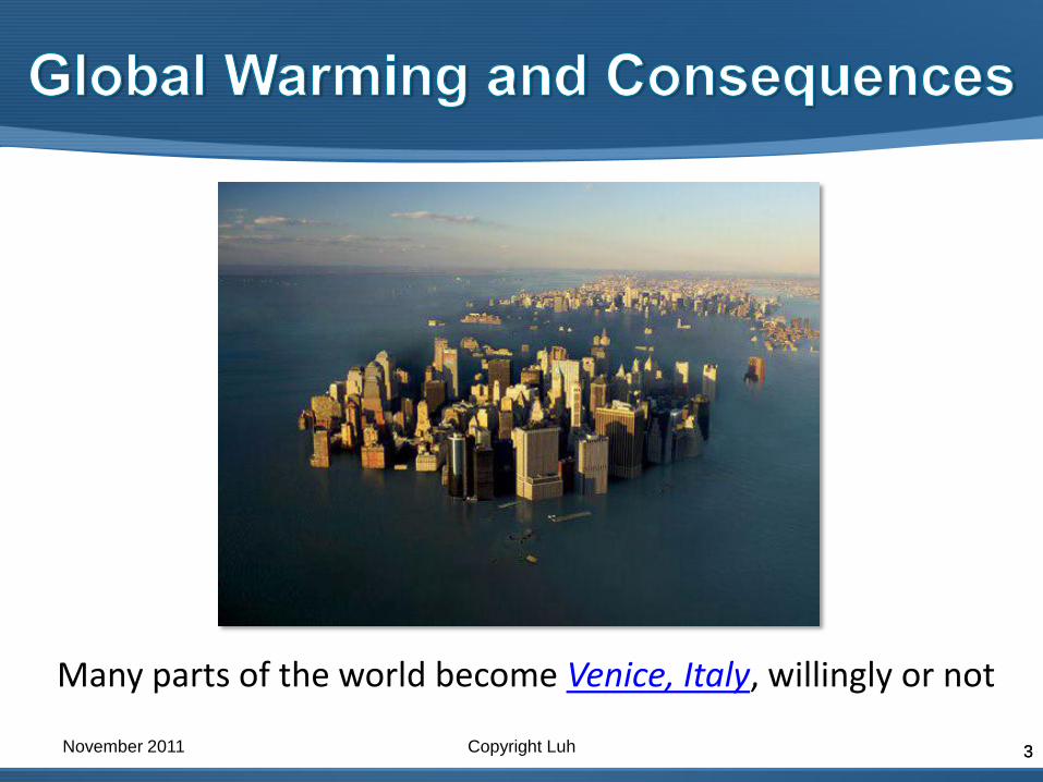
Many parts of the world become Venice, Italy, willingly or not

3

4 4

Yes, but missing a major piece of the answer

What is that? November 2011 Copyright Luh


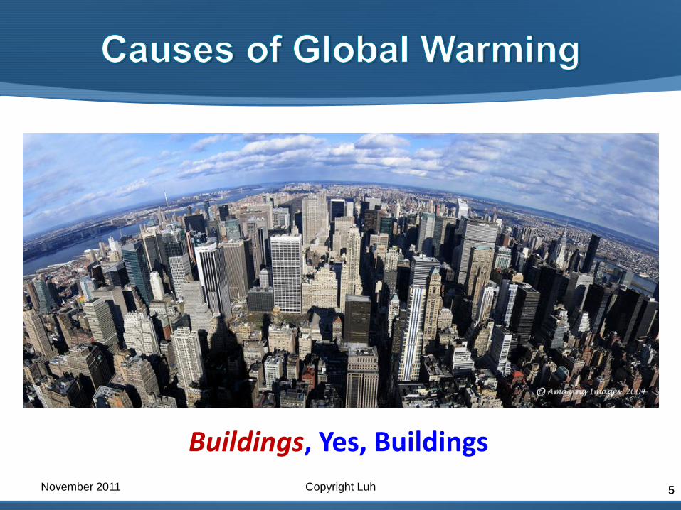
Buildings, Yes, Buildings

5


• Commercial and residential buildings are the basis of our social and economic infrastructure

• In the US, buildings are responsible for

38% of carbon dioxide emissions

71% of electricity consumption

39% of energy use

12% of water consumption

40% of non-industrial waste

• We spend 90% of our time indoors, and the indoor environment affects our health and productivity

Green, Secure, and Safe Buildings!!

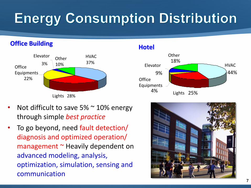
7 7

• Not difficult to save 5% ~ 10% energy through simple best practice

• To go beyond, need fault detection/ diagnosis and optimized operation/ management ~ Heavily dependent on advanced modeling, analysis, optimization, simulation, sensing and communication

Office Building

HVAC 37%

28%

Office Equipments

22%

Elevator

3% Other 10%

Lights

Hotel

44%

25% 4%

9%

18%

Lights

HVAC

Office Equipments

Elevator

Other

9

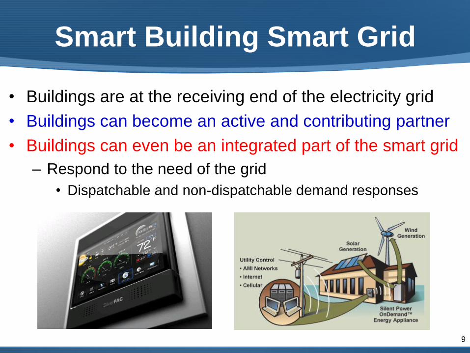
Smart Building Smart Grid

• Buildings are at the receiving end of the electricity grid

• Buildings can become an active and contributing partner

• Buildings can even be an integrated part of the smart grid

– Respond to the need of the grid

• Dispatchable and non-dispatchable demand responses

• Reduce electricity usage through fault detection,

diagnosis and optimized operation of HVAC and other

systems

• Provide infrastructure for plug-in hybrid cars and

distributed/renewable generation

• Microgrid – A new mode of power system operation

10

Actual utilization of coal fired electrical energy in China

Coal mining loss

Transmission & distribution loss Coal shipping loss

Thermal turbine loss

Actual utilization

70%

1% 1%

20% 8%

Magnifying effect

of saving energy

Courtesy of

Xiaohong

Guan,

CFINS,

Tsinghua U. 11

12 12

Smart Building

Smart Integration

Smart Grid

Temperature

Light

Sound

Motion

Sensing

Energy Management

Sensor Node Diagnosis

Report

Health Prognosis

Data Capture

Health Monitoring

Technology

• Sensor networks

• Communication

• Device integration

• Optimization

• Scheduling

• Cyber security

• Node placement

• Diagnosis

• Prognosis


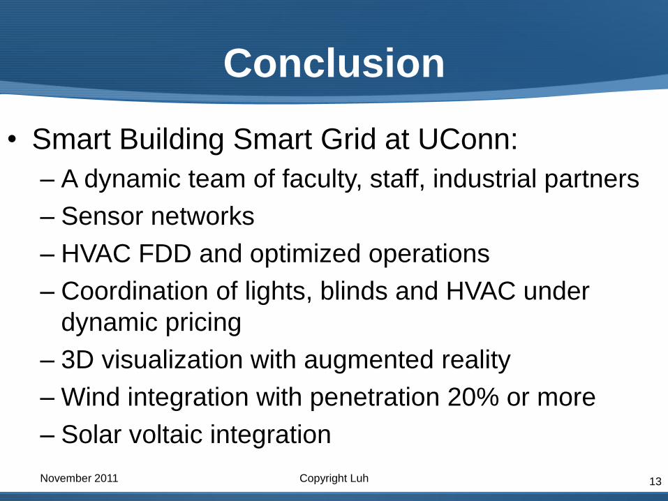
Conclusion

• Smart Building Smart Grid at UConn:

– A dynamic team of faculty, staff, industrial partners

– Sensor networks

– HVAC FDD and optimized operations

– Coordination of lights, blinds and HVAC under

dynamic pricing

– 3D visualization with augmented reality

– Wind integration with penetration 20% or more

– Solar voltaic integration


Conclusion

– Load forecast in the era of smart grid

• Won UConn School of Engineering

competition of $170k equipment

– A test bed: UConn’s Information Technology

Engineering Building under retro-commissioning

– A donation of Savant building automation system

– Another test bed: The new Engineering building

to be designed

• A meaningful and promising research area

1

Building Energy Doctor:

SPC and Kalman Filter-based Fault Detection

Biao Suna, Peter Luha, b,c, Zheng O’Neillc, and Fangting Songd

aCenter for Intelligent and Networked Systems (CFINS), Tsinghua University, China

bDepartment of Electrical and Computer Engineering, University of Connecticut, USA cUnited Technology Research Center, USA

dUnited Technology Research Center, China

Proceedings of the 2011 IEEE Conference on Automation Science and Engineering,

Trieste, Italy, August 2011, pp. 333-340. A revised version will be submitted for journal

review soon

Background and Objective

The problem: Simple and robust fault detection method

at the system level for HVACs with potential for large-

scale implementation

Is this problem important?

Buildings account for nearly 40% of global energy

consumption and 21% of greenhouse gas emissions

HVAC consumes up to 40% of energy costs of buildings

HVAC receives most complaints from building tenants

(elevators ranked the remote second)

The research represents a major opportunity for a

greener world and happier tenants

2

An HVAC system HVAC systems usually consist of multiple interconnected

subsystems – AHUs (Air Handling Units), chillers, cooling

towers, pumps, ducts, etc.

3

Cooling towers

Chillers

AHUs

Rooms

Pump

Fan

Supply airReturn airFresh airExhaust air

Supply chilled waterReturn chilled waterSupply cooling waterReturn cooling water

AHU: Use chilled water to cool and dehumidify return air and fresh air

Chiller: Produce chilled water for AHUs by transferring excess heat from

chilled water to cooling water

Cooling tower: Transfer excess heat from cooling water to outside air

Difficulties of fault detection

HVAC systems are large in scale, with many coupling

subsystems, could be building/equipment specific, and

with major uncertainties

4

Large in scale

Many coupling

subsystems

Building/equip.

specific

Uncertainties

• Fault detection methods should be fast and sensitive, e.g., only 1 of the 4 chillers has a fault

• Fault detection methods should be generic for HVACs with different manufacturers or models

• Do not need long training times for different buildings

• Effects of faults might propagate from one subsystem to another

• Fault detection methods should be robust (high detection rate and low false alarm rate) to the uncertain weather and cooling load

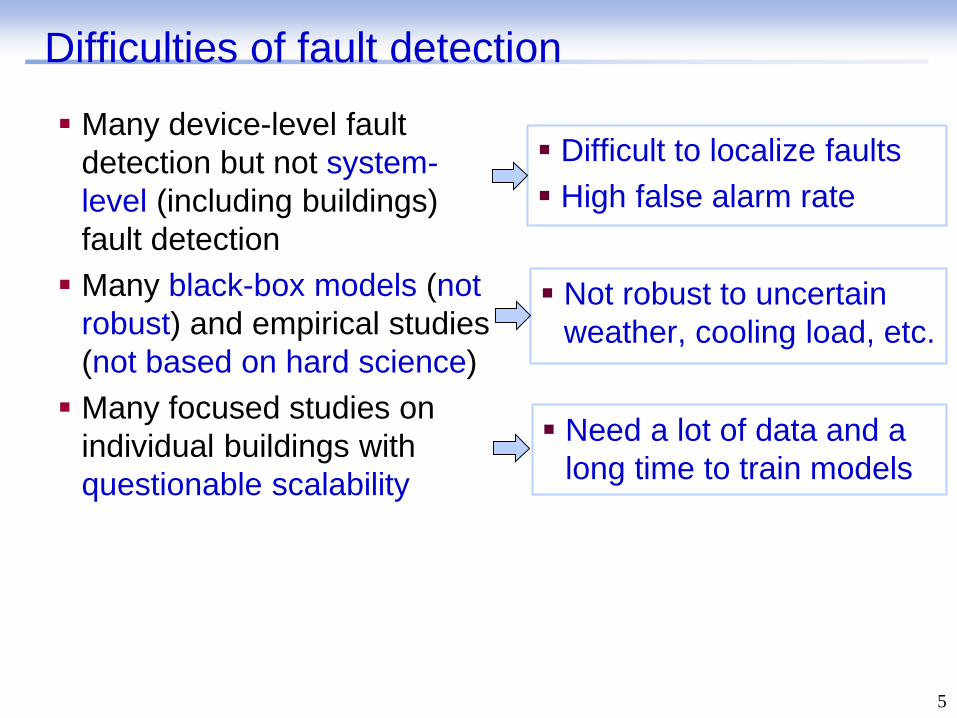
Difficulties of fault detection

Difficult to localize faults

High false alarm rate

5

Many device-level fault

detection but not system-

level (including buildings)

fault detection

Many black-box models (not

robust) and empirical studies

(not based on hard science)

Many focused studies on

individual buildings with

questionable scalability

Need a lot of data and a

long time to train models

Not robust to uncertain

weather, cooling load, etc.

Approach

Our Approach: Develop gray-box model-based and data-

driven methods with insights and understanding for robust

system-level fault detection

A novel integration of 3 simple and proven techniques

Statistical Process Control – Measuring and analyzing

variations

Kalman filters – Providing predictions and adaptive

thresholds based on gray-box models of subsystems for

robustness

System analysis – Analyzing fault propagations across

subsystems through "coupling variables"

Example: Chiller fault propagating to cooling towers

6

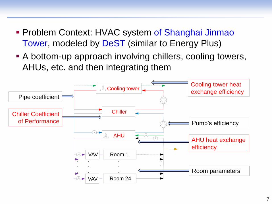
Problem Context: HVAC system of Shanghai Jinmao

Tower, modeled by DeST (similar to Energy Plus)

A bottom-up approach involving chillers, cooling towers,

AHUs, etc. and then integrating them

7

AHU heat exchange

efficiency

Pump’s efficiency

Cooling tower heat

exchange efficiency

Chiller Coefficient

of Performance

Pipe coefficient

Room parameters

Cooling tower

Chiller

AHU

Room 1 . .

.

.

.

.

.

.

.

.

.

.

VAV

Room 24 VAV

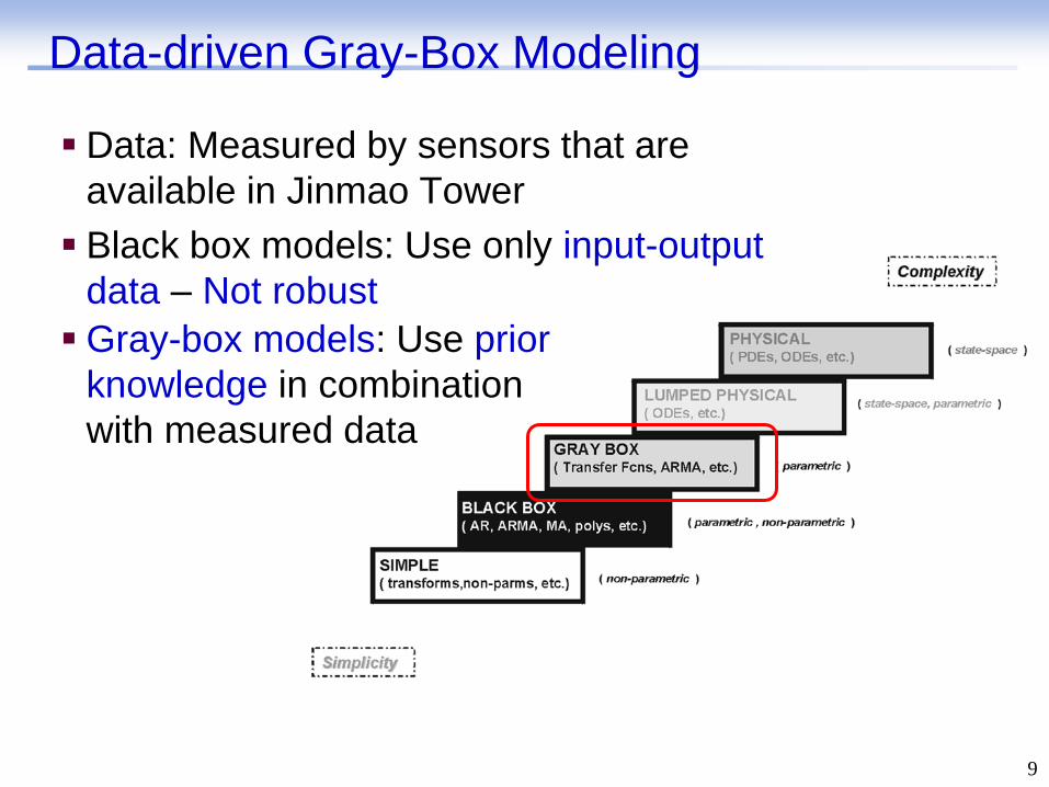
Data-driven Gray-Box Modeling

9

Data: Measured by sensors that are

available in Jinmao Tower

Black box models: Use only input-output

data – Not robust

Gray-box models: Use prior

knowledge in combination

with measured data

Gray-Box Modeling of Chillers

Reddy, et al., 2003

COP: Coefficient of Performance = qch/P (electrical power)

a1 = DS, internal entropy production rate

a2 = qleak, the rate of heat losses or gains

a3 = R, heat exchanger thermal resistance

The state: xk = [a1k, a2k, a3k]T, and xk+1 = xk + wk

Measurement: Left hand side of the above equation

Not a standard heat exchange model for chillers

10

cdi

ch

chcdi

chrcdi

ch

chr

cdi

chr

t

LCOP/a

Lt

tta

L

ta

t

t

COP

1111

1321

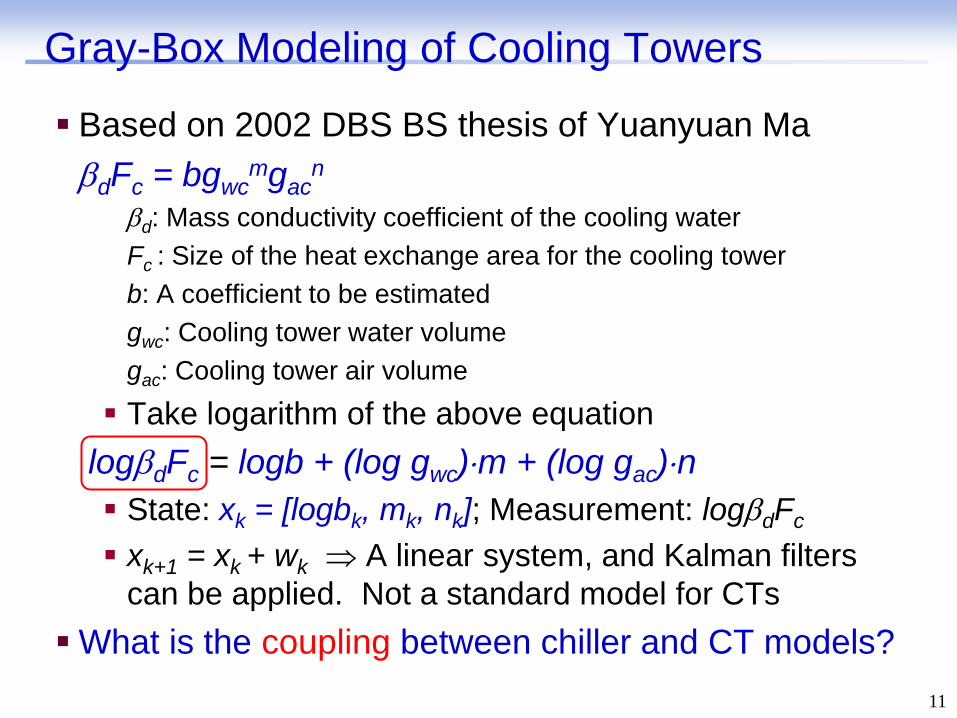
Gray-Box Modeling of Cooling Towers

Based on 2002 DBS BS thesis of Yuanyuan Ma

dFc = bgwcmgac

n d: Mass conductivity coefficient of the cooling water

Fc : Size of the heat exchange area for the cooling tower

b: A coefficient to be estimated

gwc: Cooling tower water volume

gac: Cooling tower air volume

Take logarithm of the above equation

logdFc = logb + (log gwc)m + (log gac)n

State: xk = [logbk, mk, nk]; Measurement: logdFc

xk+1 = xk + wk A linear system, and Kalman filters

can be applied. Not a standard model for CTs

What is the coupling between chiller and CT models?

11

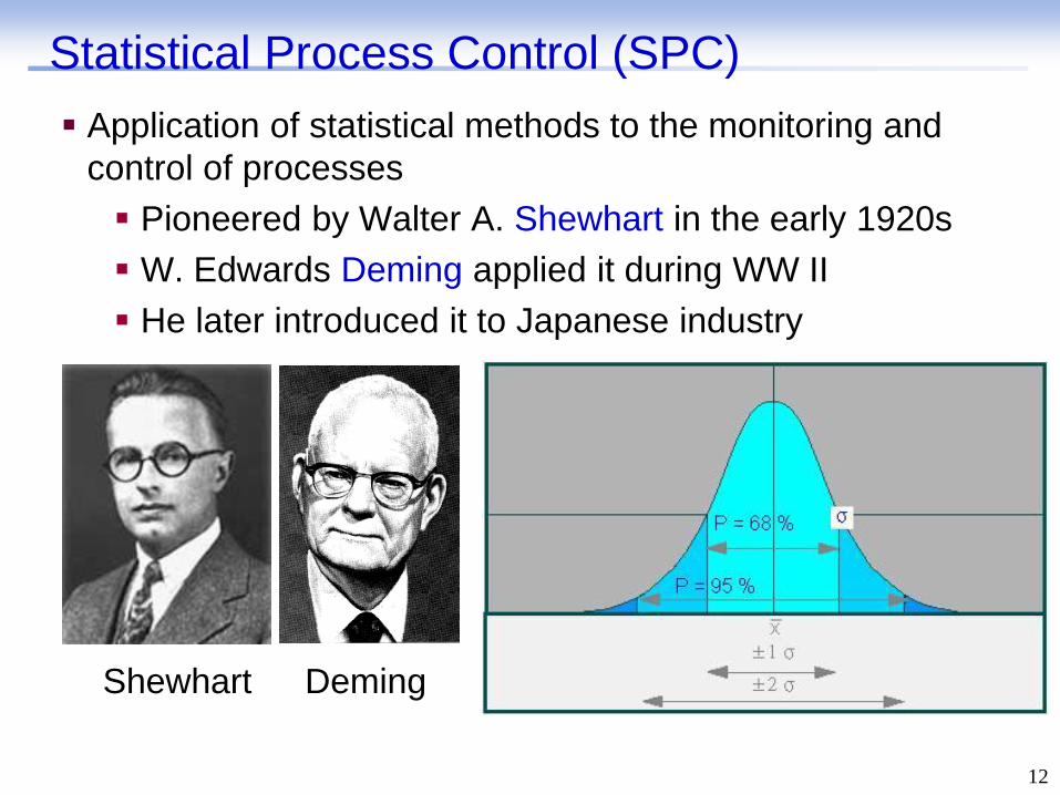
Statistical Process Control (SPC)

Application of statistical methods to the monitoring and

control of processes

Pioneered by Walter A. Shewhart in the early 1920s

W. Edwards Deming applied it during WW II

He later introduced it to Japanese industry

12

Shewhart Deming

http://en.wikipedia.org/wiki/File:WalterShewhart.gif

http://en.wikipedia.org/wiki/File:W._Edwards_Deming.gif

13

A well proven technology in manufacturing

Control limits: Based on static process capabilities

Good for HVAC fault detection?

Statistical Process Control (SPC)

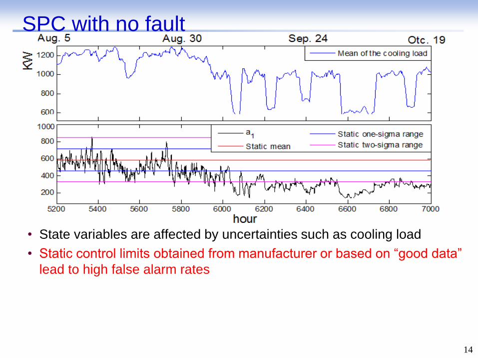
SPC with no fault

14

• State variables are affected by uncertainties such as cooling load

• Static control limits obtained from manufacturer or based on “good data”

lead to high false alarm rates

Kalman Filtering

A method to estimate the state of a process,

minimizing the mean of the squared error xk+1 = Axk + Buk + wk, p(w) ~ N(0, Q)

zk = Hxk + vk, p(v) ~ N(0, R)

15

National Medal of Science, 2009 –

from Apollo missions to GPS

Rudolf E. Kalman,

1960 Measurement update:

Bayes rule

xk+1|k+1 xk|k

Time update:

Linear systems

xk+1|k

k k+1

16

A systematic way to derive state covariance matrices and

therefore standard deviations with minimal MSE

Our idea on fault detection applications – Use Kalman

filters to predict system states and set adaptive SPC

control limits

Our Idea on Fault Detection

Adaptive control limits: 1-sigma and 2-sigma ranges

Two-sigma range: Mean ± (2×standard deviation)

How to set the mean, for example, of a1?

The mean should be the average of a1 when there is no fault. It is to

be used as a baseline for fault detection

It should be adaptively adjusted with uncertainties, e.g., cooling load

Our idea: The mean is adaptively adjusted as the average over the

past K (e.g., 24) hours

– Two sigma range (a1 in the chiller model as an example)

An SPC rule: A fault is detected if n back-to-back points of a

parameter fall outside the two-sigma range

17

1, 1, 1, 1, 1, 1,

1

1ˆ2 , 2 ,

k

k k k k k i

i k K

where aK

, same for 1,k

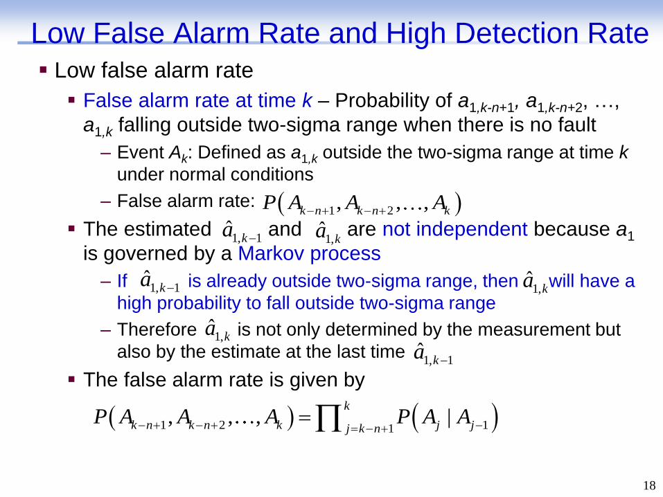
Low False Alarm Rate and High Detection Rate Low false alarm rate

False alarm rate at time k – Probability of a1,k-n+1, a1,k-n+2, …,

a1,k falling outside two-sigma range when there is no fault

– Event Ak: Defined as a1,k outside the two-sigma range at time k

under normal conditions

– False alarm rate:

The estimated and are not independent because a1

is governed by a Markov process

– If is already outside two-sigma range, then will have a

high probability to fall outside two-sigma range

– Therefore is not only determined by the measurement but

also by the estimate at the last time

The false alarm rate is given by

18

1 2, , ,k n k n kP A A A

1, 1ˆ

ka 1,ˆ

ka

1 2 11, , , |

k

k n k n k j jj k nP A A A P A A

1, 1ˆ

ka 1,ˆ

ka

1,ˆ

ka

1, 1ˆ

ka

Low False Alarm Rate and High Detection Rate Low false alarm rate

Need to find how is affected by

– By substituting the state equation into estimation, we have

– Assuming KjH is a diagonal matrix for simplicity, is given by

Assuming m1 = 0.5, false alarm rate is approximately given by

19

n back-to-back

points

False alarm rate

(Two-sigma range)

False alarm rate

(One-sigma range)

1 6.71% 33.45%

2 1.50% 15.50%

3 0.34% 7.41%

4 0.08% 3.61%

1ˆ ˆ1j j j j j j jx K H x K Hx K Hv

1,ˆ

ja1, 1ˆ

ja

1,ˆ

ja

1, 1, 1, 1 1, 1, 1, 1ˆ ˆ1j j j j j j ja m a m a m v

Low False Alarm Rate and High Detection Rate High detection rate

Detection rate can be calculated similarly as false alarm rate

Detection rate is affected by the magnitude of a fault

– Assuming a sudden fault at time k causes a1 to change form 1,k

to (1,k + s1, k )

Simulation results are good

20

SPC rule:

• Three back-to-back points

outside two-sigma range

• K = 24 to calculate the

means

0 2 4 6 8 10 120

0.2

0.4

0.6

0.8

1

Hours delayed for fault detection

Dete

ction r

ate

s=3

s=4

s=5

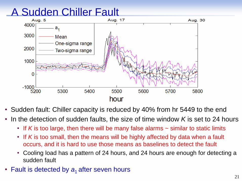
A Sudden Chiller Fault

21

• Sudden fault: Chiller capacity is reduced by 40% from hr 5449 to the end

• In the detection of sudden faults, the size of time window K is set to 24 hours

• If K is too large, then there will be many false alarms ~ similar to static limits

• If K is too small, then the means will be highly affected by data when a fault

occurs, and it is hard to use those means as baselines to detect the fault

• Cooling load has a pattern of 24 hours, and 24 hours are enough for detecting a

sudden fault

• Fault is detected by a1 after seven hours

Means should be

averaged over 30 days to

reduce the impact of false

data on the baseline.

The fault is detected after

12 days and 4 hours

A Gradual Chiller Fault

22

• Gradual fault: Chiller capacity is gradually reduced by 40% over a month from hr 5449

• How to select K to detect gradual fault?

• K should be determined based on the no. of hours the fault lasts and its

magnitude to keep a balance between quick detection and low false alarm rates

• For the above-mentioned gradual fault, K is set to 30 days

Means are averaged over

the past 24 hours.

The fault is not detected

because means are

affected too much by the

false data and cannot be

used as baseline

Fault detected False alarms

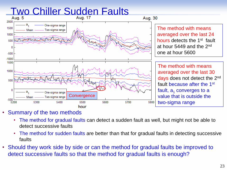
Two Chiller Sudden Faults

23

• Summary of the two methods

• The method for gradual faults can detect a sudden fault as well, but might not be able to

detect successive faults

• The method for sudden faults are better than that for gradual faults in detecting successive

faults

• Should they work side by side or can the method for gradual faults be improved to

detect successive faults so that the method for gradual faults is enough?

The method with means

averaged over the last 24

hours detects the 1st fault

at hour 5449 and the 2nd

one at hour 5600

The method with means

averaged over the last 30

days does not detect the 2nd

fault because after the 1st

fault, a1 converges to a

value that is outside the

two-sigma range

Convergence

Improve the SPC rule for successive faults

24

Key idea: Adaptively adjust the size of the time window, K, to

detect successive faults

1. Set K to Kini for initialization based on the number of hours gradual

faults last and the magnitude of faults

2. If a fault is detected, K is set to 24 so that the means can be

adjusted quickly and converged inside the two-sigma range as

soon as possible

3. After converges inside the two-sigma range at time kc, K at time

k is set to the minimal value of (k-kc) and Kini to detect the 2nd fault

1,ˆ

ka

1,ˆ

ka

5200 5300 5400 5500 5600 5700 5800-500

0

500

1000

1500

2000

hour

a

1

Mean

One-sigma range

Two-sigma range

2nd fault detected

Step 2 Step 1 Step 3 Step 2 Step 3

Fault Propagation: System-Level Fault Detection

The effects of a fault may propagate from one device

to another. This, however, doesn’t mean that other

devices are faulty too

Straightforward ideas for system-level detection

Combine gray-box models of subsystems to form an

“combined model”

Estimate the combined state by Kalman filters

Perform Statistical Process Control

Better ideas?

What are the couplings among subsystems? Then?

Can the SPC-KF fault detection framework for devices

be extended? With or without a major increase in

complexity?

25

System-Level fault detection via SPC and KF

In previous models, flows of water and air are

parameters as opposed to input, output or state

Propagation of effects from one device to another should

not directly affect the state of the latter one

“Coupling variables” are identified for system-level fault

detection

26

Chiller Fault: CT load;

CT mixed water inlet

temperature -

“Computable” based

on chiller variables

and “measurable”

within CTs

Cooling tower

Chiller

AHU

Room 1 . .

.

.

.

.

.

.

.

.

.

.

VAV

Room 24 VAV

In view of no direct coupling among gray-box models,

the overall state can be estimated by using Kalman

filters for individual subsystems developed before

No need to create a new and large Kalman filter

SPC is performed on state variables and the

difference between measured and computed coupling

variables (errors)

Standard deviations for errors can be derived for SPC

use, and the extension is with simplicity and scalability

By examining the combined system, we can tell if

there is a fault in a device or it is just the effects of a

fault propagated from somewhere else

27

28

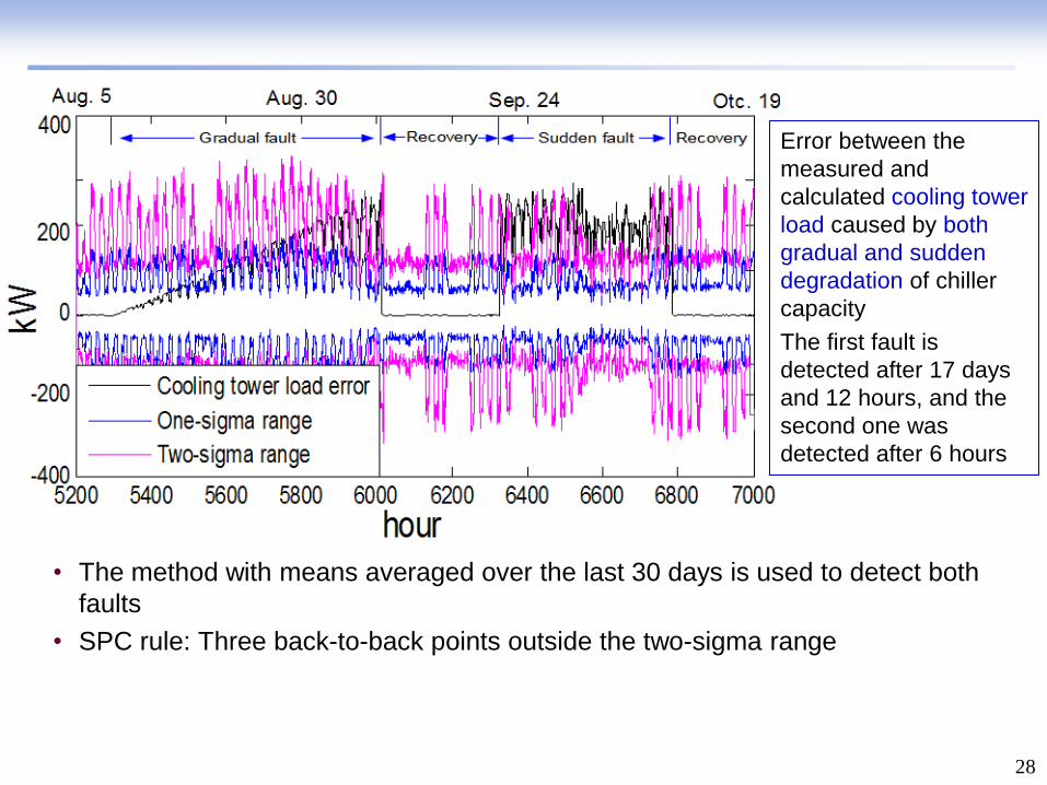
• The method with means averaged over the last 30 days is used to detect both

faults

• SPC rule: Three back-to-back points outside the two-sigma range

Error between the

measured and

calculated cooling tower

load caused by both

gradual and sudden

degradation of chiller

capacity

The first fault is

detected after 17 days

and 12 hours, and the

second one was

detected after 6 hours

Conclusion

The method is simple, and is based on a novel

combination of proven techniques of SPC, KF, and

system concepts

Results are promising:

Detect both sudden failure and gradual degradation with short

time delays

Differentiate failures or their effects propagated from elsewhere

Detect both device fault and sensor fault

The method is generic and scalable, and has many

promising applications

Next: Test on a real building at UConn’s Information

Technology Engineering Building

29

Thank you

30

smart building smart grid - unina.it · pioneered by walter a. shewhart in the early 1920s w....

Documents